SS 2020

Fuzzy Data Analysis Clustering

Prof. Dr. Rudolf Kruse

Fuzzy Systems SS 2021 Lecture 8

Part4

Data Analysis

Cross Industry Standard Process forData Analysis

Example: Bank Note Analysis

Clustering: Given 200 Swiss Banknotes. How to find groups of similar banknotes? Use attributes of each banknote. Unsupervised Learning

Classification: Given a data set with 100 real and 100 counterfeit Swiss banknotes. How to separate real from counterfeit banknotes, especially for newbanknotes? Use attributes of each banknote. Supervised learning

Understanding Data is crucial:- gathering (source,…?)- description (structure,…?)- exploration (outlier,…?)- data quality (context,…?)

Understanding Data

- Noting patterns and trends Do the trends, patterns, and conclusions make sense?

- Clustering Grouping events, places and people together if they have similar characteristics

- Counting Helps to enable the researcher to see what is there by counting frequencies

- Making comparisons Establishing similarities between and within data sets

- Partitioning variables Splitting variables to find more coherent descriptions

- Subsuming particulars into the general. Linking specific data to general concepts

- Factoring Attempting to discover the factors underlying the process under investigation

- Noting relations between variables - Finding intervening variables Establish the presence and effects of variables

- Building a logical chain of evidence Trying to understand trends and patterns through developing logical relationships.

- Making conceptual/theoretical coherence Moving from data to constructs to theories through analysis and categorisation

Many more other analyses are useful…

Part4

Two Interpretations of the Research on Fuzzy Data Analysis

FUZZY data analysis = Fuzzy Techniques for the analysis of (crisp) data

In this course: Fuzzy Clustering

FUZZY DATA analysis = Analysis of Data that are described by Fuzzy Sets

In this course: Statistics with Fuzzy Data

Part4

Cluster Analysis

Clustering

This is an unsupervised learning task.

The goal is to divide the dataset such that both constraints hold:• objects belonging to same cluster: as similar aspossible• objects belonging to different clusters: as dissimilar aspossible

The similarity is measured in terms of a distance function.

The smaller the distance, the more similar two data tuples.

Definitiond : IRp × IRp → [0, ∞) is a distance function if ∀x, y, z ∈ IRp :

(i) d(x, y) = 0⇔x = y(ii) d(x, y) = d(y,x)

(identity), (symmetry),

(iii) d(x, z) ≤ d(x, y)+d(y,z) (triangle inequality).

Part4 5 /90

Illustration of Distance Functions

Minkowski family

pk

. Σ 1k

d=1

Well-known special cases from this family are

Manhattan or city block distance, Euclidean distance,

k = 1:k = 2:k → ∞ : maximum distance, i.e. d∞(x, y) = maxp

d=1 |xd − yd|.

k =1 k =2 k → ∞Part4 6 /90

Partitioning Algorithms

Here, we focus only on partitioning algorithms,• i.e. given c ∈ IN, find the best partition of data into c groups.

Usually the number of (true) clusters is unknown. However,

with partitioning methods we must specify a c-value.

Part4 7 /90

Partitioning Algorithms

Here, we focus only on partitioning algorithms,• i.e. given c ∈ IN, find the best partition of data into c groups.

Usually the number of (true) clusters is unknown.

However, in partitioning methods we must specify a c-value.

Part4 7 /90

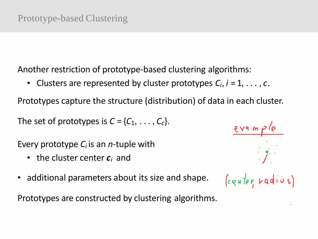
Prototype-based Clustering

Another restriction of prototype-based clustering algorithms:• Clusters are represented by cluster prototypes Ci, i = 1, ...,c.

Prototypes capture the structure (distribution) of data in each cluster.

The set of prototypes is C = {C1, ...,Cc}.

Every prototype Ci is an n-tuple with• the cluster center ci and

• additional parameters about its size and shape.

Prototypes are constructed by clustering algorithms.

Part4 8 /90

Delaunay Triangulations and Voronoi Diagrams

Dots represent cluster centers.

Delaunay TriangulationThe circle through the cornersof a triangle does not containanother point.

Voronoi Diagram Midperpendiculars of the Delaunay triangulation:boundaries of the regions of points that are closest to the enclosed cluster center (Voronoi cells).

(Hard) c-Means Clustering

1) Choose a number c of clusters to be found (user input).

2) Initialize the cluster centers randomly(for instance, by randomly selecting c data points).

3) Data point assignment:Assign each data point to the cluster center that is closest to it (i.e. closer than any other cluster center).

4) Cluster center update:Compute new cluster centers as mean of the assigned data points. (Intuitively: center of gravity)

5) Repeat steps 3 and 4 until cluster centers remain constant.

It can be shown that this scheme must converge

Part4 9 /90

c-Means Clustering: Example

Data set to cluster.

Choose c = 3 clusters.(From visual inspection, can bedifficult to determine in gen-eral.)

Initial position of cluster cen-ters.

Randomly selected data points. (Alternative methods includee.g. latin hypercube sampling)

Delaunay Triangulations and Voronoi Diagrams

Delaunay Triangulation: simple triangle (shown in grey on the left)Voronoi Diagram: midperpendiculars of the triangle’s edges (shown in blue on the left, in grey on the right)

c-Means Clustering: Example

c-Means Clustering: Local Minima

In the example Clustering was successful and formed intuitive clusters

Convergence achieved after only 5 steps.(This is typical: convergence is usually very fast.)

Nevertheless: Result is sensitive to the initial positions of cluster centers.

With a bad initialization clustering may fail (the alternating update process gets stuck in a local minimum).

The number of clusters has to be known. Some approachesfor determining a reasonable number of clusters exists.

c-Means Clustering: Local Minima

Center Vectors and Objective Functions

Consider the simplest cluster prototypes, i.e. center vectors Ci = (ci).

The distance d is based on the Euclidean distance.

All algorithms are based on an objective functions J which• quantifies the goodness of the cluster models and

• must be minimized to obtain optimal clusters.

Cluster algorithms determine the best decomposition by minimizing J.

Hard c-means

Each point xj in the dataset X = {x1, . . . , xn}, X ⊆ IRp is assigned toexactly one cluster.

That is, each cluster Γi ⊂ X .

The set of clusters Γ = {Γ1, ...,Γc} must be an exhaustive partition of X into c non-empty and pairwise disjoint subsets Γi , 1 < c < n.

The data partition is optimal when the sum of squared distances between cluster centers and data points assigned to them is minimal.

Clusters should be as homogeneous as possible.

Hard c-means

The objective function of the hard c-means isc nΣ Σ

J (X,U ,C) = uh h ij d2ij

i=1 j=1

where dij is the distance between ci and xj, i.e. dij = d(ci,xj),and U = (uij )c×n is the the partition matrixwith

iju =.

1, if xj ∈ Γi 0,otherwise

.Each data point is assigned exactly to one clusterand every cluster must contain at least one data point:

cΣ

i=1ij∀j ∈ {1, ...,n} : u = 1 and ∀i ∈ {1, ...,c} :

nΣ

j=1iju > 0.

AO Scheme for Hard c-means

(i) Chose an initial ci , e.g. randomly picking c data points ∈ X.(ii) Hold C fixed and determine U that minimize Jh:

Each data point is assigned to its closest cluster center:

uij =.

k=1 dkj1, if i = argminc

0, otherwise.

(iii) Hold U fixed, update ci as mean of all xj assigned to them: The mean minimizes the sum of square distances in Jh:

i

Σ nj=1 uijxjc = Σ n

j=1 uij.

(iv) Repeat steps (ii)+(iii) until no changes in C or U are observable.

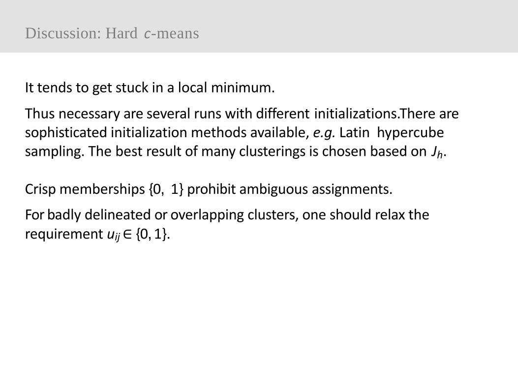
Discussion: Hard c-means

It tends to get stuck in a local minimum.

Thus necessary are several runs with different initializations.There are sophisticated initialization methods available, e.g. Latin hypercubesampling. The best result of many clusterings is chosen based on Jh.

Crisp memberships {0, 1} prohibit ambiguous assignments.

For badly delineated or overlapping clusters, one should relax the requirement uij ∈ {0,1}.

Fuzzy Cluster Analysis

Example

Given a symmetric dataset with two clusters.

Hard c-means assigns a crisp label to the data point in the middle.

That‘s not very intuitive.

In lots of cases the concept of a „fuzzy cluster“ is more intuitive.

Fuzzy Clustering

Fuzzy clustering allows gradual memberships of data points to clusters.

It offers the flexibility to express whether a data point belongs to more than one cluster.

Thus, membership degrees- offer a finer degree of detail of the data model, and- express how ambiguously/definitely a data point belong to a cluster.

Note that in the picture there are 4 clusters, the element are represented by dots ( white/black is used for visibility only) , the greyness indicates the (maximum) membership to a cluster

Fuzzy Clustering

The clusters Γi have been classical subsets so far.

Now, they are represented by fuzzy sets µΓi of X.

Thus, uij is a membership degree of xj to Γi such that uij = µΓi(xj)∈ [0,1].

The fuzzy label vector u = (u1j,...,ucj)T is linked to each xj.

U = (uij) = (u1, ...,un) is called fuzzy partition matrix.

There are several types of fuzzy cluster partitions.

Fuzzy Cluster Partition

DefinitionLet X = {x1, ...,xn} be the set of given examples and let c be the number of clusters (1 < c < n) represented by the fuzzy setsµΓi,(i = 1,...,c). Then we call Uf = (uij) = (µΓi(xj)) a fuzzy cluster partition of X if

n

Σuij > 0, ∀i ∈ {1, ...,c}, andj=1

nΣiju = 1, ∀j ∈ {1, ...,n}

i=1

hold. The uij ∈ [0, 1] are interpreted as the membership degree ofdatum xj to cluster Γi relative to all other clusters.

Fuzzy Cluster Partition

The 1st constraint guarantees that there aren’t any empty clusters.• This is a requirement in classical cluster analysis.• Thus, no cluster, represented as (classical) subset of X , is empty.

The 2nd condition says that sum of membership degrees must be 1 for each xj.

• Each datum gets the same weight compared to other data points.• So, all data are (equally) included into the cluster partition.• This relates to classical clustering where partitions are exhaustive.

The consequence of both constraints are as follows:• No cluster can contain the full membership of all data points.• The membership degrees resemble probabilities of being member

of corresponding cluster.

Fuzzy c-means Clustering

Minimize the objective function

Jf(X,Uh,C) =c nΣ Σ

i=1 j=1u dm 2

ij ijsubject to

cΣ

i=1iju = 1, ∀j ∈ {1, ...,n}and

nΣiju > 0, ∀i ∈ {1, ...,c}

where dij is a distance between cluster i and data point j,

and m ∈ IR with m > 1 is the so called fuzzifier

Objective Function The objects are assigned to the clusters in such a way that the sum of the (weighted) squared distances becomes minimal. The optimization takes place under the constraints required from a fuzzy partition.

Distance There are several options for defining the distance between a data point and a cluster. In most cases the Euclidean distance between the data point and the cluster center is used.

Fuzzifier The actual value of m determines the “fuzziness” of the classification. Clusters become softer/harder with a higher/lower value of m. Often m = 2 is chosen.

How to minimize the objective function? Some mathematical technics and tricks are necessary!

Fuzzy c-means Clustering

Reminder: Function Optimization

Task: Find x = (x1, ...,xm) such that f (x) = f (x1, ...,xm) is optimal.

Often a feasible approach is to• define the necessary condition for (local) optimum (max./min.):

partial derivatives w.r.t. parameters vanish.• Thus we (try to) solve an equation system coming from setting all

partial derivatives w.r.t. the parameters equal to zero.

Example task: minimize f (x,y) = x2 +y2 +xy − 4x − 5y

Solution procedure:• Take the partial derivatives of f and set them to zero:

= 2x +y − 4 = 0,∂x∂f ∂f = 2y +x − 5 = 0.

∂y• Solve the resulting (here linear) equation system: x = 1, y =2.

Function Optimization: Lagrange Theory

We can use the Method of Lagrange Multipliers:

Given: f (x) to be optimized, k equality constraintsCj (x) = 0, 1 ≤ j ≤ k

procedure:1. Construct the so-called Lagrange function byincorporating

Ci, i = 1, ...,k, with (unknown) Lagrange multipliers λi:kΣ

1 k i iL(x,λ ,...,λ ) = f (x) + λ C(x).i=1

2. Set the partial derivatives of Lagrange function equal tozero:

∂x∂L ∂L

∂x1 m= 0, . .., =0, ∂L

∂λ1= 0, ..., ∂L

∂λk=0.

3. (Try to) solve the resulting equationsystem.

Lagrange Theory: Revisited Example 1

Example task: Minimize f (x,y) = x2 +y2 subject to x +y = 1.

0

y1

0 0.5x

1

unconstrained minimump0 = (0,0)

minimum in the constrained subspace

2 2p1 = (1, 1)

constrained subspacex + y =1

f(x,y) = x2 +y2

The unconstrained minimum is not in the constrained subspace. At theminimum in the constrained subspace the gradient does not vanish.

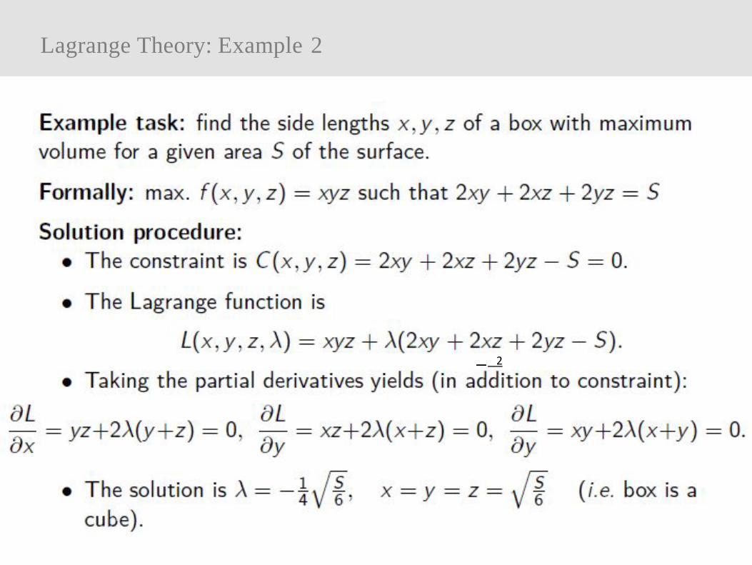
Lagrange Theory: Example 2

Example task: find the side lengths x,y,z of a box with maximum volume for a given area S of the surface.

Formally: max. f (x,y,z) = xyz such that 2xy +2xz +2yz = S

Solution procedure:• The constraint is C(x,y,z) = 2xy +2xz +2yz − S = 0.

• The Lagrange function is

L(x,y,z,λ) = xyz +λ(2xy +2xz +2yz − S).• Taking the partial derivatives yields (in addition to constraint):

∂L ∂L∂x = yz+2λ(y+z) = 0, ∂y = xz+2λ(x+z) = 0, ∂L

∂y = xy+2λ(x+y) = 0..

1 S4 6• The solution is λ = − , x = y = z =

.S6 (i.e. box is a

cube).

− 2

Alternating Optimization Scheme

Jf depends on c, and U on the data points to the clusters.

Finding the parameters that minimize Jh isNP-hard.

Fuzzy c-means minimizes Jh by alternating optimization (AO):• The parameters to optimize are split into 2 groups.

• One group is optimized holding other one fixed (and vice versa).

• This is an iterative update scheme: repeated until convergence.

There is no guarantee that the global optimum will be reached.

AO may get stuck in a local minimum.

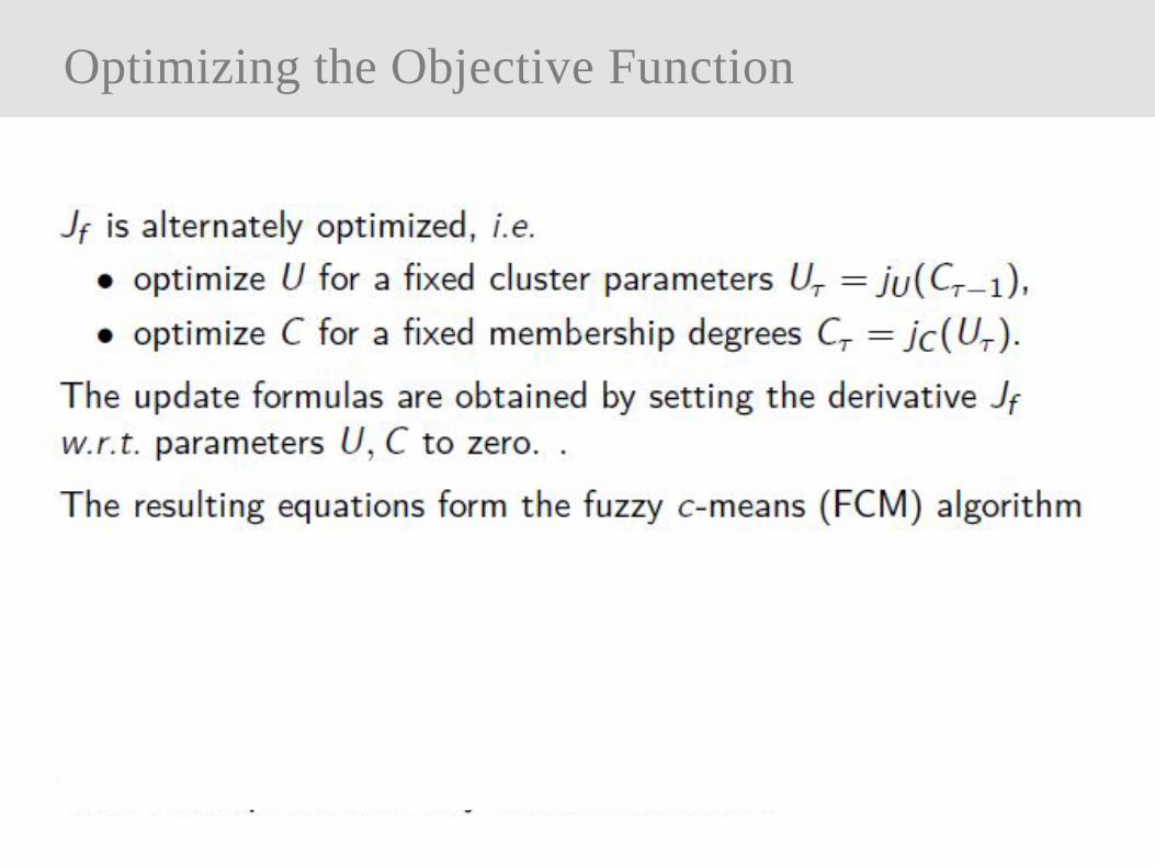
Optimizing the Objective Function

Jf is alternately optimized, i.e.• optimize U for a fixed cluster parameters Uτ = jU(Cτ−1),• optimize C for a fixed membership degrees Cτ = jC (Uτ ).

The update formulas are obtained by setting the derivative Jfw.r.t. parameters U, C to zero. .

The resulting equations form the fuzzy c-means (FCM) algorithm :

uij =1

Σ 2c dijk=1 d2

kj

. Σ 1m− 1

=d

− 2m− 1

ijΣ c d

− 2m− 1

k=1 kj

.

That is independent of any distance measure.

First Step: Fix the cluster parameters

Introduce the Lagrange multipliers λj , 0 ≤ j ≤ n, to incorporatetheconstraints ∀j; 1 ≤ j ≤ n:

Σ ci=1 uij =1.

Then, the Lagrange function (to be minimized) is

i=1 j=1ij ij

s ˛̧ xf=J(X,U ,C)

c n nΣ Σ Σ

j=1

.

L(X,Uf ,C,Λ) = umd2 + λj 1−cΣ

i=1uij

Σ

.

The necessary condition for a minimum is that the partial derivatives of the Lagrange function w.r.t. membership degrees vanish, i.e.

∂∂ukl

f klm−1 2

kl l!L(X,U ,C,Λ) = mu d − λ = 0

which leads to∀i;1 ≤ i ≤ c :∀j;1 ≤ j ≤ n : uij = λj

md2ij

1. Σm−1

.

Optimizing the Membership Degrees

Summing these equations over clusters leads

Σ

i=11 = uij =

c cΣ

i=1

λj

md2ij

1. Σm− 1

.

Thus the λj , 1 ≤ j ≤ n are. cΣ

i=1j ij

. Σ 11− m

Σ 1−m

λ = md2 .

∀i;1 ≤ i ≤ c :∀j;1 ≤ j ≤ n : uij =

Inserting this into the equation for the membership degrees yields2

d1−mij

Σ c d1−m2 .

k=1 kj

This update formula is independent of any distance measure.

Second step: Fix the Membership Degrees

The optimization of the Cluster Prototypes depends on the chosenparameters (location, shape, size) and the distance measure. So ageneral update formula cannot be given.

If the cluster center serve as prototypes and the Euclidean distancebetween cluster centers and data point are used, then the second stepyields

The two steps are performed iteratively until convergence. The algorithm finds a local minimum. Therefore the choice of different initializations are recommemded.

Example

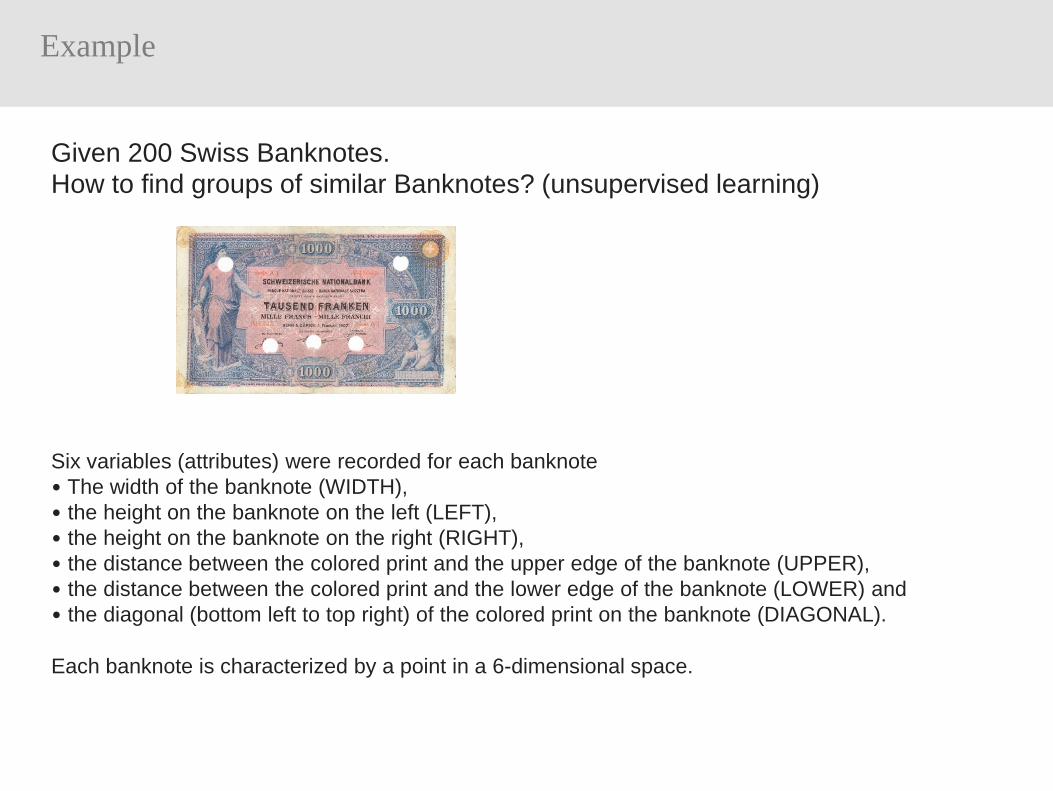
Given 200 Swiss Banknotes. How to find groups of similar Banknotes? (unsupervised learning)

Six variables (attributes) were recorded for each banknote• The width of the banknote (WIDTH),• the height on the banknote on the left (LEFT),• the height on the banknote on the right (RIGHT),• the distance between the colored print and the upper edge of the banknote (UPPER),• the distance between the colored print and the lower edge of the banknote (LOWER) and• the diagonal (bottom left to top right) of the colored print on the banknote (DIAGONAL).

Each banknote is characterized by a point in a 6-dimensional space.

Example

c-means clustering and Fuzzy c-means clustering is performed with 6-dim data

The results are presented only for the two principal components. In the fuzzy case the thickness of dots describes the membership to a respective cluster.

The clustering result of c-means (red/blue) in comparison with true classification (points below/above the diagonal) is already very good (only one misclassification).

The high uncertainty of the fuzzy algorithm near the diagonal is expressed by very small dots. In fact, the real banknotes were printed from one printing plate, while the counterfeit banknotes came from different sources and thus probably also from different forged printing plates.

Discussion: Fuzzy c-means clustering

FCM is stable and robust.

Compared to hard c-means clustering, it’s• less insensitive to initialization and

• less likely to get a bad optimization result

There are lots of real applications, case studies, implementations , theoretic results and variants of the classical fuzzy c-means algorithm.

Variants of fuzzy c-means clustering

bb Γ2bb

x1

bb bbbb Γ1

bb bb x2

x1 has the same distance to Γ1 and Γ2 ⇒ µΓ1 (x1) = µΓ2 (x1) = 0.5. The

same degrees of membership are assigned to x2.

This problem is due to the normalization.

A better reading of memberships is “If xj must be assigned to a cluster, then with probability uij to Γi”.

Variants of Fuzzy c-means clustering

The normalization of memberships is a problem for noise and outliers.

A fixed data point weight causes a high membership of noisy data, although there is a large distance from the bulk of the data.

This has a bad effect on the clustering result.

Dropping the normalization constraint

cΣuij = 1, ∀j ∈ {1, ...,n},

i=1

we obtain sometimes more intuitive membership assignments.

Possibilistic Cluster Partition

DefinitionLet X = {x1, ...,xn} be the set of given examples and let c be the number of clusters (1 < c < n) represented by the fuzzy setsµΓi,(i = 1, ...,c). Then we call Up = (uij) = (µΓi(xj)) a possibilistic cluster partition of X if

nΣuij > 0, ∀i ∈ {1, ...,c}

j=1

holds. The uij ∈ [0, 1] are interpreted as degree of representativity ortypicality of the datum xj to cluster Γi .

now, uij for xj resemble possibility of being member of corresponding cluster

Possibilistic Clustering

The objective function for fuzzy clustering Jf is not appropriate for possibilistic clustering: Dropping the normalization constraint leads to a minimum for all uij =0.

Hence a penalty term is introduced which forces all uij away from zero.

objective function Jf is modified to

Σ Σ m 2p p ij ij

c n c nΣ Σi ijJ (X,U ,C) = u d + η (1 − u ) m

Optimizing the Membership Degrees

The update formula for membership degrees is

iju =1

1+d 2

ijηi

. Σ 1m−1

.

The membership of xj to cluster i depends only on dij to this cluster.

A small distance corresponds to a high degree of membership.

Larger distances result in low membership degrees.

So, uij ’s share a typicalityinterpretation.

Interpretation of ηi

The update equation helps to explain the parameters ηi.

ijConsider m = 2 and substitute ηi for d 2 yields uij = 0.5.

Thus ηi determines the distance to Γi at which uij should be0.5.

ηi can have a different geometrical interpretation:• the hyperspherical clusters (e.g. PCM), thus √ηi is the mean

diameter.

Estimating ηi

If such properties are known, ηi can be set a priori.

If all clusters have the same properties, the same value for all clusters should be used.

However, information on the actual shape is often unknown a priori.• So, the parameters must be estimated, e.g. by FCM.

• One can use the fuzzy intra-cluster distance, i.e. for all

Γi , 1 ≤ i ≤ n

i

Σu dn m 2

j=1 ij ijη = Σ n umj=1 ij

.

Optimizing the Cluster Centers

The update equations jC are derived by setting the derivative of Jpw.r.t. the prototype parameters to zero (holding Up fixed).

The update equations for the cluster prototypes are identical. Then

the cluster centers in the PCM algorithm are re-estimated as

i

Σ nj=1 ijumxjc = Σ n um

j=1 ij.

Comparison of Clustering Results

Note that in the picture there are 4 clusters, the element are represented by dots ( white/black is used for visibility only) , the greyness indicates the (maximum) membership to a cluster

Distance Function Variants

So far, only Euclidean distance leading to standard FCM and PCM

Euclidean distance only allows spherical clusters

Several variants have been proposed to relax this constraint• fuzzy Gustafson-Kessel algorithm

• fuzzy shell clustering algorithms

Can be applied to FCM and PCM

Gustafson-Kessel Algorithm

Replacement of the Euclidean distance by cluster-specific Mahalanobis distance

For cluster Γi , its associated Mahalanobis distance is definedas

j j j i2 T −1

i j id (x , C ) = (x − c ) Σ (x − c)

where Σi is covariance matrix of cluster

Euclidean distance leads to ∀i : Σi = I, i.e. identity matrix Gustafson-

Kessel (GK) algorithm leads to prototypes Ci = (ci, Σi )

Iris Data

Iris setosa Iris versicolor Iris virginica

Collected by Ronald Aylmer Fischer (famous statistician). 150 cases in total, 50 cases per Iris flower type.Measurements: sepal length/width, petal length/width (in cm). Most famous dataset in pattern recognition and data analysis.

Classification of flowers

- Classification issupervised learning

- Visual Analysis with a Scatter plot: 4-dim Data represented in by 12 2-dim projections of labelleddata

- Automatic classification ispossible, e.g. by support vector machines

- There are also fuzzyversions of SVM

Clustering of flowers

Clustering is unsupervised learning based on unlabelled data

Testing clustering methods: Use labelled data, remove the labels of the data , cluster the unlabelled data, compare the clustering result with the original classification

Result of c-means clustering True Classificationon Unlabelled data Labelled data

Gustafson Kessel Clustering of the (unlabelled) Iris Data

Good clustering result with only few errors

Projected original labelled data

Fuzzy Shell Clustering

Up to now: searched for convex “cloud-like” clusters

Corresponding algorithms = solid clustering algorithms

Especially useful in data analysis

For image recognition and analysis:variants of FCM and PCM to detect lines, circles or ellipses

shell clustering algorithms

Replace Euclidean by other distances

Fuzzy c-varieties Algorithm

Fuzzy c-varieties (FCV) algorithm recognizes lines, planes, or hyperplanes

Each cluster is affine subspace characterized by point and set of orthogonal unit vectors,Ci = (ci,ei1, ...,eiq) where q is dimension of affine subspace

Distance between data point xj and clusteri

2j id (x , c ) = ǁ 2

qΣj i j

Tx − cǁ − (x − c ) ei ill=1

Also used for locally linear models of data with underlying functional interrelations

Other Shell Clustering Algorithms

Name Prototypesadaptive fuzzy c-elliptotypes (AFCE)

fuzzy c-shellsfuzzy c-ellipsoidal shells

fuzzy c-quadric shells (FCQS)fuzzy c-rectangular shells (FCRS)

line segments circles

ellipseshyperbolas, parabolas

rectangles

AFCE FCQS FCRS