fundamental measurement for health services research
TRANSCRIPT

FINAL REPORT -----------------
FUNDAMENTAL MEASUREMENT
FOR HEALTH SYSTEMS RESEARCH
R01 HS10186-01
Agency for Healthcare Research and Quality
William P. Fisher, Jr., PhD and George Karabatsos, PhD
Department of Public Health & Preventive Medicine
Louisiana State University Health Sciences Center
Reprint requests and all communication concerning this manuscript should be addressed to:
William P. Fisher, Jr., PhD
LSUHSC Public Health & Preventive Medicine
1600 Canal Street, Suite 800
New Orleans, LA 70112
504/568-8083
504/568-6905 (Fax)
March 1, 2001
Acknowledgements: This research was supported by grant number R01 HS10186 from the
Agency for Healthcare Research and Quality. Thanks to Robert Marier, Elizabeth Fontham, and
Bronya Keats of the LSU Health Sciences Center in New Orleans for their support of this work.
Portions of this work were presented at the Third International Outcome Measurement
Conference, held at Chicago’s Northwestern Memorial Hospital in June, 2000, and at the annual
meeting of the American Public Health Association, held in Boston, in November, 2000.
1
FUNDAMENTAL MEASUREMENT FOR HEALTH SYSTEMS RESEARCH
William P. Fisher, Jr., PhD and George Karabatsos, PhD
TABLE OF CONTENTS
Abstract 4
Introduction 5
Measurement Theory 7
Hypotheses 13
Survey Respondents and Instrument 15
Results 17
Hypothesis 1 18
Hypothesis 2 19 The Item Hierarchy 19 Instrument Targeting 23 Rating Scale Step Hierarchies 24
Hypothesis 3 25
Measure Invariance 25
Calibration Invariance 27
Hypothesis 4 28
Hypothesis 5 28
Summated Ratings 29
Item Response Theory 33
Recommendations for Instrument Improvement 41
Discussion 42
Conclusion 48
References Cited 50
Tables and Figures 57
2
Tables and Figures Table 1. Six persons’ responses to a 4-item survey 57 Table 2. The data in Table 1 expressed as probabilities 58 Table 3. Summary statistics for measures and MEPS QOC items 59
Table 4. Response category structure, items 7, 8, and 10 60 Table 5. Response category structure, items 4-6, 9, and 11 61 Table 6. Response category structure, items 1 and 3 62 Table 7. Response category structure, item 2 63
Table 8. Comparison of QOC person measures across several item-subset conditions 64
Table 9. Correlations of item calibrated on random samples, and by median split 65 Table 10. Item calibration correlation matrix 66 Table 11. ANOVA analysis of measures: Public HMO vs. Private HMO vs. Medicare 67 Table 12. Using fit statistics to identify inconsistent responses 68
Table 13. Comparison of features of PCM, IRT, and Summated Ratings analyses 69 Figure 1. Necessary & sufficient conditions: interval scaling & measurement invariance 70 Figure 2. Variable map 71 Figure 3. Most probable response plot 72 Figure 4. QOC person measures, 2 category vs. 4-category items 73 Figure.5 Comparison of item calibrations across random samples, and by median split 74 Figure 6. Comparison of item calibrations: Public HMO vs. Private HMO vs. Medicare 75 Figure 7. Plot of non-linear ratings against linear QOC measures, for item 2 76 Figure 8. Plot of scores against linear QOC measures 77 Figure 9. Plot of person scores against linear QOC measures 78 Figure 10. Plot of item scores against linear QOC item calibrations 79 Figure 11. WINSTEPS PCM vs. MULTILOG 1PL Samejima
Graded Response Model measures 80 Figure 12. WINSTEPS PCM vs. MULTILOG 1PL measures (anchored) 81 Figure 13. WINSTEPS PCM vs. MULTILOG 1PL measures (discrimination=1.8) 82 Figure 14. WINSTEPS dichotomous calibrations vs. MULTILOG 1PL calibrations 83 Figure 15. WINSTEPS dichotomous measures vs. MULTILOG 1PL measures 84 Figure 16. WINSTEPS dichotomous calibrations vs. MULTILOG 2PL calibrations 85 Figure 17. WINSTEPS dichotomous calibrations vs. MULTILOG 3PL calibrations 86 Figure 18. WINSTEPS dichotomous measures vs. MULTILOG 2PL measures 87 Figure 19. WINSTEPS dichotomous measures vs. MULTILOG 3PL measures 88 Figure 20. MULTILOG 3PL vs. MULTILOG 2PL maximum a posteriori measures 89 Figure 21. Variation in item discrimination parameter estimates by type of data input 90 Figure 22. Variation in item discrimination parameter estimates by model 91
3
FUNDAMENTAL MEASUREMENT FOR HEALTH SERVICES RESEARCH
ABSTRACT
Science advances on the basis of linear measurement systems that are invariant across
different experimental conditions. However, most survey-based health sciences research employs
measures that have never been tested for invariance. This study describes and demonstrates the
mathematical properties underlying the additive formulations of probabilistic conjoint
measurement (PCM), which provide the necessary and sufficient conditions for fundamental
measurement. As a demonstration, PCM was applied to data from 23,767 persons who responded
to the Medical Expenditure Panel Survey (MEPS) conducted by the Agency for Healthcare
Research and Quality (AHRQ; formerly the Agency for Health Care Policy and Research
(AHCPR)). This demonstration includes tests of five hypotheses: (1) that the quality of care
(QOC) variable is quantitative, (2) that the data’s ordering of the survey items and rating
categories is meaningful, (3) that the respondent measurement order remains constant over item
subsamples, and that the item calibration order remains constant over respondent subsamples, (4)
that there are no differences among the measures associated with respondents belonging to one
or another of several different forms of insurance coverage (Private HMO, Public HMO, and
Medicare), and (5) that each of three approaches to measurement (PCM, Item Response Theory,
and the commonly used method of summated ratings) have specific scientific strengths and
weaknesses that make them appropriate for general use as scientific measurement methods. None
of the hypotheses were rejected, though (3) and (5) are strongly qualified. The results indicate
two general conclusions: (1) PCM offers new insights into theories of QOC, and (2) it is possible
to construct fundamental measurement systems of QOC variables. Finally, since QOC
fundamental measurement systems can be constructed, it will be possible to equate and interpret
the responses of different QOC surveys in the same metric.
4

INTRODUCTION
“It is a scientific platitude that there can be neither precise control nor prediction of
phenomena without measurement…. It is nearly useless to have an exactly formulated
quantitative theory if empirically feasible methods of measurement cannot be developed for a
substantial portion of the quantitative concepts of the theory. Given a physical concept like that
of mass or a psychological concept like that of habit strength, the point of the theory of
measurement is to lay bare the structure of a collection of empirical relations which may be used
to measure the characteristic of empirical phenomena corresponding to the concept. Why a
collection of relations? From an abstract standpoint a set of empirical data consists of a
collection of relations between specified objects …The major source of difficulty in providing an
adequate theory of measurement is to construct relations which have an exact and reasonable
numerical interpretation and yet also have a technically practical interpretation” (Scott & Suppes,
1958).
The research reported here asks what empirical relations in quality of care survey data
might provide the measurement quality needed for both exact numerical and technically practical
interpretations. If a variable is to be measured precisely, then it needs to be 1) measurable on a
linear (interval or ratio) scale, where 2) the measurement of objects does not depend on which
measurement instrument is used, and 3) the properties of the measuring instrument do not change
with the object measured. For instance, a person's height 1) represents a linear magnitude, 2)
remains the same, no matter which ruler is used, and 3) the markings on the ruler remain in the
same positions, regardless of who is measured.
That the three basic requirements of measurement can be met in the physical sciences is
strikingly obvious. That these requirements can be attained in the health sciences is not so
obvious, since most health science variables (e.g., pain, quality of life, etc.) are latent. Common
practice assigns numeric values to observations of these variables and analyzes them as though
they represent linear magnitudes. Such assignments arbitrarily depend on the perceptions of the
5
experimenter and the particular persons surveyed. Measurements based on such assignments are
never linear or generalizable across laboratories.
For example, summed rating scale responses are typically treated as linear measures.
Consider a 3-category response format Disagree (1) / Neutral (2) / Agree (3) employed for a
particular survey. Although the assigned numbers show a difference of 1 between successive
categories, their true distances are unknown and may be highly variable (Wilson 1971; Duncan
1984; Merbitz, Morris & Grip 1989; Wright & Linacre 1989; Michell 1990, 1997, 1999, 2000;
Fisher 1993; Stucki, Daltroy, Katz, Johannesson & Liang 1996; Zhu 1996). The existence of a
single unit difference between categories is typically assumed, with no effort made at producing
supporting evidence, even though multiple studies have shown that rating categories usually are
not equally spaced. In short, there is no more justification for assuming stable category distances
of 1 than there is for assuming variable distances of 0.5 and 1.75, or 3.0 and 0.9. Experimenter-
defined numerical assignments to observations can be only ordinal, and never represent true
magnitudes. Treating ordinal data as interval or ratio has been referred to as laying the
“foundations of misinference” and is generally recognized as unscientific (Merbitz, et al. 1989).
Measurement theoreticians have shown conclusively that it is possible to construct
interval quantitative measures using ordinal information (Scott & Suppes 1958; Rasch 1960;
Luce & Tukey 1964; Andersen 1977; Wright 1977b, 1985, 1999; Falmagne 1979; Perline,
Wright & Wainer 1979; Wright & Stone 1979; Andrich 1988, 1989; Suppes, Krantz, Luce &
Tversky 1989). If ordinal data embody relationships prescribed by the axioms of additive
conjoint measurement (ACM), then measures are linearly scaleable, and are as mathematically
rigorous as physical measures. Accord with ACM axioms confirms that the relevant properties of
6

the measured objects are invariant with respect to the measurement instrument, and that the
properties of the measuring instrument are invariant with respect to the objects measured.
MEASUREMENT THEORY
Consider the case of a survey/test data set containing dichotomous responses (e.g.,
Yes/No; Agree/Disagree; True/False; Correct, Incorrect). Let n∈N represent a person from the
person set, and i∈I an item from the item set; Xni is a person-item response from the set {0,1},
and Pni1 is the probability of a Xni=1 response, 0 < Pni1 < 1. From the N×I matrix of responses, a
person's ability (βn) and an item's calibration (δi) are functions of
( )( )βn r I r≈ − ( )( )δi N s s≈ − (1a-1b)
where the "person score" r and the “item score” s are sufficient statistics for β and δ, respectively
(Andersen 1977). The set of person abilities β and item difficulties δ are obtained by
maximizing the likelihood function
( )( ) ( )L X P Pni N I niX
ni
X
i
I
n
Nni ni
×
−
=== −∏∏β δ, 1 1
1
111 (1c)
See Wright & Masters (1982) for a survey of various maximum likelihood estimation algorithms.
ACM can be expressed probabilistically (Rasch 1960; Falmagne 1979; Perline, et al.
1979; Wright 1985; Andrich 1988; Suppes, et al. 1989; Wright & Linacre 1989) with a model
that specifies the log-odds (λni1) of a Xni=1 response as an additive function of βn and δi:
( )n P Pni ni ni n i1 0 = = −λ β δ (2)
where ( )[ ]Pni11
1= + −−
exp λ (3)
7
and ( ) ( )[ ]P Pni ni0 11
1 1= − = +−
exp λ (4)
It can be inferred from (2-4) that (λni1 > 0) ⇒ (Pni1 > .5), (λni1 < 0) ⇒ (Pni1 < .5), and
(λni1 = 0) ⇒ (Pni1 = .5).
The process at which the model relates to the N×I response matrix is illustrated by the
following example. Table 1 shows a hypothetical data set created by six persons responding to a
four-item survey. Persons and items are ordered by total score, and the set of person abilities β
and item calibrations δ are estimated by (1a) and (1b), respectively. This ordering
approximates a pattern of overlapping triangles of 1s and 0s in the response matrix. An exception
that proves (tests) the rule is provided by person f who unexpectedly endorsed z, the most
difficult item, despite having a low score. Unexpected responses such as this provide
opportunities for data quality assessment and improvement, and can stimulate construct
clarifications by raising questions as to whether all respondents and items belong to the same
respective populations (Wright 1977b; Wright & Stone 1979; Wright & Masters 1982; Smith,
Schumacker & Bush 1998).
Since survey responses occur probabilistically and not deterministically, it is useful to
evaluate the observed data matrix as response probabilities. Table 2 presents the person-item
responses as a Pni1 matrix, obtained through substitution of the corresponding β and δ values into
(3). The responses of persons a, b, c, d, and e agree with the model. In each of these cases,
responses coded as 1 occurred when Pni1 > .50, and responses coded as 0 occurred when Pni1 <
.50. The responses of persons c and d to items x and y contain a mix of 0 and 1 responses,
plausible events considering Pni1=.50. The surprising "1" response of person f to item z has a .06
probability. The low probability follows from the fact that this person’s measure (-1.1) is almost
three logits below the item’s calibration (1.6). The improbability of this observation indicates a
8

contradiction of the measurement intention, and would require further investigation into possible
data entry errors, sampling, or construct issues.
Why is it necessary for data to approximate modeled probabilities? For convenience,
consider persons a and b in measure group p, c and d into group q, and e and f into group r, as
shown in the left side of Figure 1. The β estimates specify that the person relations are p > q > r,
and the δ estimates specify that the item relations are w > x = y > z. According to the matrix of
Pni1 values, the person order p > q > r is preserved for all items, and the item order w > x = y > z
holds for all person measures. In other words, the person measurement order is invariant,
regardless which items are used for measurement, and the item calibration order is invariant,
regardless of which persons are measured. Removing responses to items w and y still preserves
the Pni1 order of p > q > r for all i, and removing responses from persons with measure p
preserves the Pni1 order for w > x = y > z for all n. These properties satisfy the independence
axiom of ACM, a condition that requires person measurement to be free from the properties of
the measuring instrument, and the properties of the measuring instrument remain invariant no
matter which persons are measured.
Though measurement invariance is attained by data adhering to the independence axiom,
this property alone does not transform ordinal observations into interval measures. All measures
at the quantitative (interval/ratio) level have additive characteristics, so both double cancellation
and independence are needed for additivity. Double cancellation is illustrated in the right of
Figure 1: Since the antecedents (px > qz and qw > rx) and the consequent (pw > rz) are satisfied,
the probability matrix satisfies double cancellation.
Because of their additive formulations, probabilistic conjoint measurement (PCM)
models always specify response probability matrices that satisfy independence and double
9
cancellation. PCM's approach is analogous to ANOVA, in that the axioms require "person" and
"item" factors to produce additive and non-interactive effects on the response probabilities. Item
curves (based on Pni1 across β) must be parallel with equal slopes. Item response theory (IRT)
models that do not specify such curves cannot produce measures with invariance properties
(Andrich 1988, 1989; Cliff 1989, 1992; Fisher 1994; Karabatsos 1999a, 1999b; Wright 1984,
1999). Although models that allow item curves to cross (Hambleton & Swaminathan 1985) may
be appealing for their accommodation of inconsistent data, the very fact that their structure
contradicts the three basic measurement requirements renders goodness-of-fit analysis irrelevant
(Karabatsos 1999a). One class of these models takes the formulation αi (βn - δi), where αi is the
slope of the item characteristic curve at βn = δi (Hambleton & Swaminathan 1985). Such item
"weighting" violates independence by distorting the conjoint order of response probabilities (e.g.,
Table 2). These models thus inherently entail sample-and test-dependent measurement.
The degree to which measurement objectivity is attained depends on how well data
accord with the measurement principles specified in a PCM model. The standardized response
residual represents the basis for all item and person fit statistics:
Z x E Wni ni ni ni= −( )2 (5)
where Xni is the observed response, and Eni is the expected response, and Wni is the variance of
the expected response. For dichotomous responses, Eni = Pni1 and Wni = Pni1(Pni0). Zni is expected
to approximate a N(0,1) distribution. The fit of person and item response sets is calculated using
mean-square statistics (MS), which have an expectation of 1. Outfit mean-square (OMS) is the
average Z2 across responses:
OMS Zni= ∑ ∑2 1 (6)
a statistic very sensitive to extreme unexpected responses, i.e., when βn >> δi or βn << δi . Infit
10

mean-square is more sensitive to unexpected responses for close βn and δi distances:
IMS W Z Wni ni ni= ∑ ∑2 (7)
In common practice, MS>1.3 diagnoses an item or person with inconsistent responses; MS<.7
signals overfit, an improbable degree of consistency. Type I error rates for MS statistics are
available using the null hypothesis of data-model fit (Smith 1988, 1991; Smith, et al. 1998).
Misfitting items and persons are usually set aside for subsequent analyses, since such data
distort the transitivity among person ($) measures and item calibrations (*). This step in the
calibration of a measurement system has been controversial (Goldstein & Blinkhorn 1977;
Goldstein 1979; Gustafsson 1980; Phillips 1986; Smith 1986), largely because its focus on the
validity of the construct goes against the grain of traditional true-score measurement theory,
which places higher value on content validity (Fisher 1994; Cherryholmes 1988; Messick 1975).
Because data are commonly deemed valid on the basis of a test or survey’s content, the standard
paradigm has been to fit models to data, rejecting the model when it does not fit the data. From
within this paradigm, changing the data, or the way in which observations are made, in order to
obtain model fit has been viewed as an artificially contrived and unethical tampering necessarily
unacceptable in scientific work.
But when data are too inconsistent to calibrate a ruler, the researcher should not give up
and make do with data that will not support scientific generalization, which is what is often
currently recommended (van der Linden & Hambleton 1997). When data must be removed from
the process of calibrating an instrument, the item or person involved is not simply deleted.
Rather, the characteristics of that item or person are examined for reasons why the measurement
effort failed (Wright 1977b, 1999; Wright & Stone 1979; Woodcock 1999). Is the item
ambiguously phrased, or does it offer more than one interpretation? Does the item perhaps
11

belong to a different construct that ought to be measured with its own instrument? Was there a
data entry error? Was this person mistakenly sampled from a different population, as might be
inferred from particular response patterns shared by an identifiable subsample that shares a
consistency different from the rest of the sample? Did the respondent mistakenly reverse the
rating scale options? Far from being a mindless trashing of data, explanations of these kinds open
the door to improving the quality of the data and the precision and accuracy of the measuring
instrument.
The degree to which measurement objectivity is attained is also a function of
measurement reliability. As a part of model fit optimization, it is also useful to evaluate how well
item calibrations discriminate among the measured persons, and vice-versa, using separation (G)
statistics (Wright & Masters 1982). The person separation (Gn) ratio describes the number of
performance levels that the test distinguishes in the sample of respondents; the item separation
(Gi) ratio indicates how well items spread along the variable. G is calculated by:
G = ASD / RMSE (8)
where RMSE (root mean square error) is the error variance of the measures, and ASD is the
standard deviation of the measures adjusted for RMSE, or
ASD2 = SD2 - RMSE2 . (9)
The relationships between the Kuder-Richardson reliability statistic (R) and separation is
R = G2 / (1+G2) G = [ R / (1 - R) ]1/2 . (10)
In principle, either R or G can be used. G is more descriptive, since 1) every unit increase
represents an equal increment of change in the ratio of variation to error, and 2) G has an infinite
range, 0 < G < +∞, while the range of R is constrained in [0,1].
12

HYPOTHESES 1 The first hypothesis tests whether the data support the contention that the quality of care
variable is quantitative (Michell 1990). The quantitative hypothesis will be rejected or
provisionally confirmed via tests of model fit, the extent to which the data satisfy the
requirements of independence and double cancellation (Luce & Tukey 1964; Krantz, et
al. 1971; Michell 1990, 1997), as implemented in a probabilistic conjoint measurement
(PCM) model (Brogden 1977; Perline, et al. 1979; Wright 1985, 1997). Experimental
procedures for maximizing model fit will be demonstrated in detail.
2 Provided satisfactory model fit is established, then the hypothesis that meaningful
substantive relations are associated with hypothesis 1’s quantitative structure can be
tested. The fundamental issue of interest is construct validity. The empirical item order
on the scale is examined in order to answer the question, “Do the data arrange the MEPS
QOC item estimates reasonably and meaningfully, so that services with low calibrations
are easy to be satisfied with, services with high calibrations are difficult to be satisfied
with, and persons with low measures are less satisfied than those with high measures?”
3 Following the investigation of construct validity, the person measures and item
calibrations will be checked for robustness via analyses of randomized and
demographically defined sub-samples of the data. The hypotheses tested will require that
person measures be the same (linearly convertible, with at least a .85 correlation) no
matter which particular items are used to produce them, and that the item calibrations
remain the same no matter which particular persons respond to them. Item calibration
robustness will establish that very large samples are not needed for many measurement
and scale development tasks, and that item difficulty order and the substantive meaning
of the measures can be interpreted as generally characteristic of the population. Person
13

measurement robustness will demonstrate that 1) missing data can be accommodated, 2)
measurement technology can be adapted to the needs of the respondent, instead of
requiring respondents to adapt to the needs of the technology (Choppin 1968; Lunz,
Bergstrom & Gershon 1994), and 3) different instruments measuring the same variable
could be equated to measure in a single reference-standard quantitative metric (Fisher
1997a, 1997b, 1998, 2000a). If broadly realized in health services research, robust
measures could greatly improve the efficiency and meaningfulness of that research, as
well as its implementation.
4 Fourth, as an elementary demonstration of the use of PCM logits in a statistical analysis,
the QOC measures are studied submitted to an analysis of variance to test an hypothesis
concerning variation in amounts of QOC across public and private HMOs, and Medicare.
Do persons paying more for their health care experience substantially higher QOC?
5 Fifth, PCM will be evaluated relative to summated ratings and IRT analyses of the same
MEPS QOC data. PCM, IRT, and the summated ratings approach are all often used in
practice as though they produce interval measures; this study will evaluate the extent to
which the results of each actually meet the long-established requirements for fundamental
measurement applications in science and commerce, as articulated by Campbell (1920),
Fisher (1922), Guttman (1950), Rasch (1960), Luce and Tukey (1964), (Suppes, Krantz,
Luce & Tversky (1989), and others, as summarized by Michell (Michell 1990, 1999,
2000) and Wright (Wright 1999).
14

SURVEY RESPONDENTS AND INSTRUMENT
A PCM model was applied to data from 23,767 families who responded to the Medical
Expenditure Panel Survey (MEPS), conducted by the Agency for Healthcare Research and
Quality (AHRQ; formerly the Agency for Health Care Policy and Research (AHCPR)) (Cohen,
et al. 1996-97). The dataset (HC-002) used in these analyses was downloaded from the AHRQ
website in 1998. The analysis focused on 11 survey items pertaining to quality of care (QOC),
listed below (item response options are shown in parentheses). Earlier questions in the interview
establish the identity of the persons obtaining care from a particular provider. The provider’s
name is then used in the following questions, and pronouns (they, them) refer to the persons
seeking care.
1. [AC17] How difficult is it to get appointments with your provider on short notice, for
example, within one or two days? (Very / Somewhat / Not too / Not at all Difficult)
2. [AC18] If they arrive on time for an appointment, about how long do they usually have to
wait before seeing a medical person? (>2 hrs./1-2 hrs./31-59 mins./16-30 mins./5-15
mins./<5 min.)
3. [AC19] How difficult is it to contact a medical person at your provider over the telephone
about a health problem? (Very / Somewhat / Not too / Not at all Difficult)
4. [AC19A] Does your provider generally listen to them and give them the information needed
about health and health care? (No/Yes)
5. [AC19b] Does the provider usually ask about prescription medications and treatments other
doctors may give them? (No/Yes)
6. [AC19C] Are they confident in the provider's ability to help them when they have a medical
problem? (No/Yes)
15

7. [AC19D] How satisfied are they with the professional staff at the providers’ office? (Not at
all / Not too / Somewhat / Very Satisfied)
8. [AC19E] Overall, how satisfied are they with the quality of care received from the provider?
(Not at all / Not too / Somewhat / Very Satisfied)
9. [AC24] During the last year, did any family member not receive a doctor’s care or
prescription medications because the family needed the money to buy food, clothing, or pay
for housing? (Yes/No)
10. [AC24A] Overall, how satisfied are you that members of your family can get health care if
they need it? (Not at all / Not too / Somewhat / Very Satisfied)
11. [AC25] In the last 12 months, did anyone in the family experience difficulty in obtaining
care, delay obtaining care, or not receive health care they thought they needed due to any of the
reasons listed on this card [list of 18 reasons shown to respondent]? (Yes/No)
In the original AHRQ documentation, these items are included in the Access to Care (AC)
section of the household survey. With each question, respondents were given the opportunity to
say they did not have an answer. Note that the set of items employ four different groups of rating
categories, three of which use rating scale options. Therefore, for this experimental design, it is
necessary to employ a different PCM model for each rating scale, which can be expressed as:
( )λ βni j j k nijk ni j k n i jkn P P( , ) ( )− −= = −1 1 δ τ− (11)
where τ is the response threshold between response category j and j-1, k is the rating category
group (k={1,2,3,4}), and λni(j,j-1)k is the log-odds of response category j being chosen versus
category j−1.
It is also important to notice that the rating scales differ in the direction they point. The
original coding of item 1 above, for instance, assigned a rating of 1 to very difficult, indicating
16

low QOC, and a 4 to not at all difficult, indicating high QOC. With the very next question in the
interview, however, the direction of the coding is reversed, such that waiting times of less than
five minutes are rated as 1, and waits of more than two hours, 6.
In order to evaluate the capacity of the ordinal observations to support interval
measurement, the ratings need to consistently point in the same direction, so that any rating in a
higher category always indicates more QOC. The data were therefore recoded so that a high sum
of ratings for a respondent would indicate the overall high QOC associated with a high measure,
and a high sum of ratings for an item would indicate that it represents the relatively low QOC
hurdle that calibrates toward the bottom of the scale. The order of the codings as they were
employed in the analyses is shown in the listing of the items above.
Accordingly, scoring the one 6-point item (2), the five 4-point items (1, 3, 7, 8, and 10),
and the five dichotomous items (4, 5, 6, 9, and 11) as consecutive integers, 1-6, 1-4, and 1-2,
respectively, results in a minimum possible score of 11, and a maximum possible score of 36,
given complete data (responses to all items).
RESULTS
The following results are provided by the PCM program WINSTEPS (Wright & Linacre
1999). Table 3 shows the summary statistics for the 23,767 cases, of which 208 lacked
responses, 3,383 obtained the maximum score of 36, and 165 obtained the minimum score of 11,
leaving 20,011 analyzable cases. Persons and items with maximum and minimum scores are not
analyzable because they provide no information as to their position on the scale, being, in effect,
shorter than the first unit on the ruler, or taller than the last unit.
17

The top part of Table 3 provides a global summary of person (top) and item (bottom)
statistics. The item scale is centered at zero (refer to the mean ITEM MEASURE). The average
person measure of 2.08 is therefore over two errors (0.85) above the center of the scale,
indicating that, relative to the administered items, the sample receives high QOC. The average
REAL ERROR for the persons is .85, and is .02 for the items. The small item calibration error is
due to the large sample size. As the number of measures increases and the unit of measurement is
successfully repeated, error decreases, variation remains constant or increases, and reliability
increases.
Hypothesis 1: The Quality of Care variable is quantitative
The first hypothesis is not rejected. As shown in Table 3, on average, the person and item
fit statistics are satisfactory, although the variance and range of the mean-square statistics
indicate that there are some persons with unexpected responses. In general, however, the
independence and double cancellation axioms are not violated. As is described in greater detail
under Hypothesis 3a, below, a series of experiments were conducted in order to determine the
instrument’s optimal characteristics.
In these experiments, model fit was not markedly improved, since it was satisfactory at
the start. Modeled reliability was improved from .65 to .82, but this seems to have been inflated
by the appearance of a nearly 3-logit gap in the middle of the item calibration distribution. The
effect of the gap in the item calibrations on the respondent measures would be to increase
variation without simultaneously increasing error; hence the increase in reliability. A less
extreme removal of inconsistent observations resulted in no change in reliability, equivalent
model fit, and improved construct definition, as presented below.
18

Hypothesis 2: The Quality of Care items and rating categories fall in a meaningful order and
position relative to the measures
This hypothesis is taken up under the subheadings of the overall item hierarchy, the
instrument targeting, and the rating scale step hierarchy.
The Item Hierarchy. The second hypothesis is not rejected. Figure 2 provides important
information about the QOC construct. The positions of the measures and calibrations in this
figure are taken from the first analysis of all measurable 20,011 cases. After these are described,
they are compared with the results of the optimized analysis.
The item at the bottom of Figure 2’s variable map involves the provider’s ability to listen
to the patient and provide relevant information. Immediately above this item are two others
involving the family’s ability to obtain care, and confidence in the provider. These issues
constitute the overriding purposes of the encounter, so it seems of some theoretical importance
that the measurement of QOC would start here.
At the other end of the scale, at the top of Figure 2, are items concerning waiting time,
phone access, and making appointments. Respondents are least likely to rate these items in high
categories, suggesting that only the highest quality care providers will receive positive responses
in these areas. It is of some interest to note that the items are distinguished along the
measurement continuum by general and specific expressions of QOC. With the exception of the
easiest item, the bottom seven items are relatively abstract, while the top four involve specific
services provided. This contrast should prove of theoretical value in the development of
improved QOC instruments.
19
Since a higher person measure indicates higher QOC, the probability of satisfaction
decreases as item calibrations increase. To illustrate, hypothetical responses from fictional
people named “Tom,” “Mary,” and “Cindy” were inserted into Figure 2. Mary’s position on the
QOC variable (above 6) indicates that she is likely to be satisfied with or agreeable relative to all
the items. Cindy’s position (at about –2) on the variable indicates that she is not likely to be
satisfied with any of the items. Tom’s position (≈0) indicates that he is likely to be very satisfied
with or agreeable relative to items 4, 6, and 9, not satisfied with 2, 3, 1, and 5, with about a .50
probability that he is satisfied with 10, 7, 11, and 8.
When all items fit a PCM model, and are ordered in a meaningful hierarchy, they all
measure the same variable. Failures of invariance are invitations to investigate construct validity,
with the aim of better understanding and improving the item hierarchy. The MEPS QOC items 2
and 5 provoke responses that are less consistent (MS > 1.2) than the other items’ responses. The
other items involve issues that are crucial components of QOC, addressing basic issues of access,
provider skill, and information availability. In contrast, responses to questions concerning
appointment waiting time (item 2), and whether the provider asks about other treatments (item
5), do not vary with the same consistency as the other items in the scale. From the perspective of
item fit, the MS statistics suggest that these two items are not consistent components of the
unidimensional QOC construct, and should therefore be set aside for subsequent analyses.
These two items should not automatically be considered ineffective, and mechanically
deleted from further consideration. They might 1) be inordinately affected by only a very few
especially unexpected responses from persons with extremely high or extremely low measures;
2) be useful for measuring a different unidimensional aspect of QOC; or 3) signal the existence
of a special respondent subsample especially interested or uninterested in these aspects of QOC.
20

Perhaps the item "Provider asks about other treatments" is relatively more important for a group
of respondents who have particular conditions with well-known alternative treatments, or for
persons with multiple co-morbidities who may be at risk for medication interactions.
And it may be impossible for certain high-QOC patients to have short waiting times in
the particular clinics they visit. It could be that these clinics are crowded because of the high
quality care they deliver. No matter whether response inconsistencies occur as systematic
functions of persons or items, further investigation of the standardized residuals (as calculated in
equation 5) is warranted. Factor analysis of the standardized residuals appears to be an approach
that is useful for detailed construct investigations (Wright & Linacre 1999; Linacre 1998).
An alternative to setting aside noisy persons/items is the removal of individual responses
(single person-item interactions) with high residuals. This is possible since the probabilistic
properties of PCM models enable the handling of missing data with little or no consequence to
person and item measurements, even though greater numbers of missing responses necessarily
increase the error of measurement. Employing this strategy on these data caused the removal of
all responses in the most positive category of the most difficult item, involving waits of less than
five minutes to see the doctor at appointments. Responses in this extremely positive category
were so improbable that they were inherently inconsistent with all other responses. Removing
them then caused the item to become less difficult and its relative position shifted from the top of
the hierarchy to fourth from the top. In addition, the spread of the other items on the variable
increased from about 3 logits to over 7 logits. Almost all of that change, however, was
introduced in the form of a gap between the top four and bottom seven items, suggesting that the
elimination of the waiting time and other treatment inconsistencies set the stage for a clearer
21
expression of the difference between the more agreeable, general aspects of the construct at the
bottom of the scale, and the less agreeable, specific aspects at the top.
The advantage of removing individual inconsistent responses is that the analyst is able to
retain as much information as possible from the data set, without the unreasonable dependence
on complete person-response sets. For most other approaches to measurement, a missing
response leads to the deletion of a person or item from the analysis, or the application of some
test-dependent scoring algorithm to replace the missing response(s) (Bernhard, et al. 1998; Hahn,
Webster, Cella & Fairclough 1998; Troxel, Fairclough, Curran & Hahn 1998). Within the PCM
framework, if it is of concern that missing responses occurred as a function of non-random
factors, then the item calibrations can be compared across respondent groups exhibiting different
amounts or types of missing responses, in order to detect item bias.
The person-item variable map is considered from a different perspective in Figure 3,
which shows the expected responses across all of the items for individual measures. The
distribution of all measures is shown at the bottom of the figure, with the number of measures at
each point along the logit ruler indicated by the vertical columns of numbers. There are, for
instance, 2,004 measures at the mean (about 2.1 logits), indicated by the M at the bottom of the
figure (S indicates one SD; T, two).
To take a specific example, Tom, who measures about 0 on the QOC scale, is expected to
have a response string, listed in item difficulty order (from the bottom up), of 22232331222
(Tom’s expected responses are underlined in Figure 3). Mary, who experiences higher QOC and
a measure of about 4, is expected to respond 2224442445 (Mary’s expected responses are
circled.) The various patterns of responses associated with each possible score-measure
combination constitute the modeled expectations against which observations are compared.
22
Because the modeled expectations of consistent variation embody the criteria of
sufficiency, Guttman reproducibility, conjoint additivity, and parameter separation (Wright
1999), the difference between those expectations and the observations is of primary value in the
estimation of model fit. When any given measure is associated with a model fit statistic in a
satisfactory range, observations and expectations conform to one another sufficiently well for the
measure, understood as effective within a range defined by plus or minus two errors, to be
interpreted as meaningfully approximating the ideal.
Accordingly, Figure 3 could be used as the basis for a redesigned assessment form. For
instance, clinician managers could use this type of figure as an assessment form (i.e.,
KEYFORM) to measure and qualitatively assess QOC at the point of care (Connolly, Nachtman
& Pritchett 1971; Fisher, et al. 1995a; Linacre 1997; Ludlow & Haley 1995; Ludlow, et al. 1992;
Sparrow, Balla & Cicchetti 1984; Woodcock 1973, 1999). To obtain a patient’s QOC measure,
the patient simply responds to the questions by circling the appropriate categories, and the
provider then draws a line through roughly the middle of the circled responses, and refers to the
patient’s measure (and error, raw score, percentile rank, or whatever other statistic might be
deemed relevant and worth including) at the bottom of the form. Once the analyst has reached
the point at which item calibrations are stable, calibrated forms can be provided to physicians,
nurses, and other care providers as diagnostic tools. This is one method of integrating
measurement methodology with clinical practice, making the enhanced interpretability
established via instrument calibration immediately available at the point of care with no need for
further time-consuming computerization and data analysis.
Instrument Targeting. The mistargeting of items to persons is illustrated in the person-item
variable map in Figure 2, and in Figure 3. More than 61% of the sample is likely to be satisfied
23

with every item (β>1.75), and more than 90% persons measure above the center of the item scale
(δ=0). Given the instrument’s 36 response categories, Rasch generalizability theory (Linacre
1993) predicts a measurement error of about .50 for an on-target sample, in contrast to the
present sample’s .85 average error. With an average measurement error of .50 and this sample’s
measurement standard deviation of about 1.4, one would then expect a person measurement
separation of about 2.7 and associated reliability of .88.
Figure 2 shows only the average step difficulty for the items. For the items with
dichotomous, yes-no response formats, the sole step difficulty is the same as the item difficulty.
But for the five items rated on multicategory scales, calibration estimates are obtained at each
step transition. The construct definition and the instrument targeting are then enhanced, in this
case only slightly, by the additional information provided by the rating scale step estimates, as
shown in Figure 3.
Rating Scale Step Hierarchies. Four different groups of response categories were calibrated. For
the purposes of this demonstration, attention will be focused on the “Very Satisfied / Somewhat
Satisfied / Not Too Satisfied / Not At All Satisfied” rating scale of items 7, 8, and 10. The
analysis of its rating scale structure is provided in Table 4. The “Observed Count” column
summarizes the number of responses made within each rating category, and the “Average
Measure” column indicates the average person measures responding to each category. The
results are satisfactory, as an increasing score on the rating scale corresponds to an increase in
both the average measures and the category thresholds. Both MS statistics indicate that there are
some unexpected "1" responses, which suggests that the two misfitting items contain responses
of 1 when their expected ratings were much higher.
24
The figure at the bottom of Table 4 illustrates that the category response thresholds (Jjk)
correspond to the locations where curves j and j-1 cross. Therefore, -.55 is the response threshold
between categories 1 and 2, -.42 is the threshold between categories 2 and 3, and .98 is the
threshold between categories 3 and 4, as indicated in Table 4, which means that a higher QOC
rating contributes to higher patient QOC measure, as intended.
Results for the remaining items’ step structures are shown in Tables 5-7 and are in
general satisfactory. Overall, the data exhibit, item by item and step by step, the conjoint
response pattern expected by the PCM model. But notice that each of the three rating scales
includes one very small step, suggesting that it may be necessary to collapse adjacent ones
together.
Collapsing categories is recommended when (a) category responses exhibit statistically
significant inconsistencies (MS>1.2), (b) a category has a low observed count, (c) most of the
category’s response curve lies under an adjacent category's curve, or (d) when the size of the step
from the previous category is less than 1.4 logits (Linacre 1999). Such an optimization of the
rating scale usually improves fit, and will also improve separation/reliability to the extent that
error is lowered relative to variation. In this case, an experimental recoding the data resulted in
the elimination of statistically significant inconsistencies, and had no effect on
separation/reliability.
Hypothesis 3a: Measures are invariant across item subsamples
Hypothesis 3a is not rejected, but provisionally, with a strong need for improved data
quality. The person separation statistic for the initial analysis of all 20,011 available cases
indicates that there is about as much error variance as measurement variance (Gn=1.17), as is
25

associated with low person reliability (R=.58). In other words, the highest measure cannot be
distinguished from the lowest measure to a statistically significant degree because the instrument
lacks the power it needs to spread the respondents out along a number line. In order to give
numeric expression to quantitative magnitudes, an instrument should discriminate 2+
measurement levels of QOC (Gn >2, Rn> .80). High stakes applications can require reliabilities
above .95, as is required for consistent and reliable reproduction of a measure across instruments.
It is sometimes possible to establish an instrument’s maximum possible reliability by
removing cases with significant inconsistencies (OMS > 1.4), or with significant amounts of
missing data. After the instrument’s best performance is observed, the cases that had been
removed are replaced, and measures for them are produced by anchoring the items at their
established calibrations. If the error introduced by the inconsistencies or the missing data
decreases relative to the variation in the measures, reliability increases.
With the MEPS QOC data, however, iterative analyses removing ultimately 9,999 cases
exhibiting the strongest inconsistencies had negligible effect on the measurement reliability
coefficient. The main effect of these analyses was to remove cases with responses at the extreme
low end of the rating scale for the item involving appointment waiting times (i.e., persons
indicating that they had waited over two hours before seeing a doctor). This in turn caused the
item to drift progressively lower down the scale from its original position as the most difficult
indicator of QOC to a new position fourth from the top. In these analyses, the positions of the
other items remained stable, but the mistargeting of the instrument was exacerbated, with the
mean measure increasing from 2.08 to 3.18.
Figure 4 shows the results of a direct test of measurement invariance across item
subsamples. These results were produced by dividing the QOC items into two groups defined by
26

the number of available response categories, and using these as separate instruments each
measuring the QOC experienced by the entire (second, reduced) sample of respondents. The
overall correlation between the two sets of measures is .71.
Further tests of this hypothesis are summarized in the correlations shown in Table 8.
Three subsets of items, chosen based on their difficulty calibrations (low, medium, and high),
and two mutually exclusive random sets of items, were calibrated in separate WINSTEPS
analyses on the original data set’s 20,011 measurable cases. Correlations range from about .26 to
.89. The lowest values are associated with comparisons of item groups that vary greatly in their
difficulties (low vs. high), and the highest values, with groups of items that are similar in
difficulty (middle, high, and the two random selections).
Overall, the low number of items available for scaling makes it difficult to obtain highly
reliable measures. Were there more items, and had they been designed with the intention of
establishing invariant measures in mind (i.e., taking up the recommendations of Fisher (2000b)
and others), larger subsets of more reliable items would be available, and better able to provide
measures in a uniform metric. To obtain the same measure using different brands or
configurations of instruments known to measure the same thing would require that the
correlations be higher and the associated plots would show a narrower range of variation nearer
to the identity line.
Hypothesis 3b: Calibrations are invariant across respondent subsamples
Hypothesis 3b is not rejected, since the item calibrations spread along the scale very well
(Gi =51, Ri=1.0). As a demonstration of the scale invariance over respondent subsamples, data
from five randomly chosen (with replacement) groups of respondents, and from two other groups
27

distinguished by their measures (high and low), were used to produce seven separate sets of item
calibration estimates. Sample sizes for the randomly selected groups were 500, 250, 100, with
two other groups of 35. The sample sizes of the high median and low median groups were 4,915
and 6,094, respectively.
Correlations for these groups of item difficulty estimates are shown in Table 9; the values
correlated are plotted in Figure 5. Sixteen of the 21 correlations (about 80%) are greater than or
equal to .84, and about half of them (10 of 21) are over .90. With the exception of the item at the
far right of Figure 5, involving difficulty in receiving health care, the items calibrate in the same
order across samples, even with sample sizes as low as 35.
A similar pattern and similar correlations, here averaging about .95, were produced by
respondent subsamples defined by their participation in public or private HMOs, or in Medicare
(see Table 10 and Figure 6).
Hypothesis 4: Measures do not vary across demographic groups
This traditional statistical hypothesis of no difference in measures across groups is
rejected on the basis of a significant F-test (see Table 11). In substantive measurement terms,
however, the differences in the mean measures are very small (0.06, 0.27, and 0.33 logits), with
all of the differences less than half the average estimated measurement error (.85 for the total
sample). In other words, when the differences in the measures are interpreted in terms of an
actual change in responses to the questions asked, no such change is seen as likely.
Hypothesis 5: PCM, IRT, and summated ratings are each appropriate in QOC measurement
Though retainable in certain limited respects, overall, this hypothesis has to be
rejected. The superior data quality assessment and interval measurement characteristics of PCM,
28

relative to IRT and summated ratings, are irrefutable. A summary of PCM, IRT, and summated
ratings features is provided in Table 13. We will now take up a more detailed examination of
summated ratings and IRT analyses of the MEPS QOC data.
Summated Ratings. Reconsidering again Figure 3, we see that not only are the distances between
adjacent categories variable, but the position of a given category on the ruler changes with the
difficulty of the items. Figure 7 shows another view of the data shown in Table 7 for the MEPS
QOC item 2, involving waiting time for an appointment. The distances between the step
thresholds reported in Table 7 are shown in Figure 7 in such a way that the “foundations of
misinference” (Merbitz, et al. 1989) on which so much research is based become graphically
apparent. For instance, a change in waiting times that would be expressed as a shift in the
average response from 2.5 to 3.5 raw score units corresponds with a one-logit difference on the
measurement scale, but the same single unit shift from 4.5 to 5.5 in the expected score
corresponds with more than three logits on the measurement scale.
Figures 8-10 display other ways in which the nonlinearity of ordinal scores is misleading.
Figure 8 plots the entire range of possible scores (11-36), given complete data, against
their logit-linear transformations (the approximate β estimates for the minimum score 11 and the
maximum score 36 are based on hypothetical scores of 11.3 and 35.7). The relationship takes the
shape of an ogive since scores are always bounded by their minimum and maximum values,
while their associated logit estimates range from -4 to +4. Figure 8 shows the consequences of
using nonlinear raw scores for statistical inference. A 2-point difference from 21 to 23 translates
to a 1-logit increase, but the same 2-point gain from 32 to 34 is a 2-logit increase. Hence, the
score difference between 32 and 34 is quantitatively twice more than the apparently equal
difference between 21 and 23.
29
The crux of Likert’s (1932) argument against Thurstone was that, with complete data, the
middle of the score distribution is nearly additive. The problem that is especially pertinent to the
mistargeted MEPS QOC instrument is that the natural logarithm’s two-stretch transformation of
the score distribution causes the size of a raw score unit to vary by up to 400% on the logit
metric (Wright 1999) depending on where that unit is positioned. That is, the difficulty of
advancing a single score unit at the extreme ends of the measurement continuum is much more
challenging than it is in the middle of the ruler. Raw scores from different parts of the ruler are
almost always compared with no cognizance of this difference, so the inferences made are
inherently flawed.
Figures 9 and 10 show plots of all raw scores versus their associated logit measures for
the measures and calibrations, respectively. These figures highlight the effect of missing data on
the raw scores. Notice that the upper edge of the points plotted in Figure 9 represents the same
complete-data curve shown in Figure 8. The points below that upper edge represent score groups
formed on the basis of responses to fewer than all of the available questions on the instrument.
Although competent users of survey instruments know better than to compare raw scores
summed from different collections of questions, this plot draws attention to the inconvenience of
methods unable to account for missing data, and the advantages of odds ratios as a component of
fundamental measurement theory and practice for adapting instruments to the needs of people,
instead of forcing people to adapt to the needs of instruments.
Without checking the internal consistency of the data, users of the summated ratings
approach also have no means of determining whether raw scores are sufficient statistics, or if
important information about the variable is left embedded in interactions hidden in the data.
Unfortunately, reliability statistics are often mistakenly interpreted as measures of internal
30

consistency (Green, Lissitz, & Mulaik 1977; Ottenbacher & Tomchek 1993), and the more
appropriate mean square model fit statistics (Smith, Schumacker, & Bush 1998) are rarely used.
Table 12, taken from the WINSTEPS output, lists the MEPS QOC items provoking the
least consistent responses. As shown in Figure 2, the items with the highest OMS (Outfit Mean
Square) statistics, concerning items 5 (the provider’s questions about other treatments), and 2
(appointment waiting time), calibrate in the upper half of the difficulty distribution, at 0.66 and
1.59 logits, respectively. Two particularly unexpected responses of 1 (No) to item 5, the worst
fitting item, stand out in Table 12. These responses come from respondents 21388 and 21387 (as
can be seen by reading the vertical column of numbers immediately above the responses in Table
12).
Respondents 21388 and 21387 provided identical answers to all questions, and have the
same measure of 3.5, IMS of 3.3, and OMS of 9.9, based on responses to all 11 items and raw
scores of 34. Table 12 also shows that these same two persons also responded in category 6 to
item 2, indicating that they typically wait less than five minutes to see the doctor when they
arrive on time for an appointment. An additional inconsistency indicated in Table 12 are the
responses of No to question 9, concerning the ability of everyone in the family to obtain needed
care. Examination of an additional table available in the WINSTEPS output indicates that these
are the only observations affecting these two respondents’ measures to a statistically significant
degree.
Referring again to Figure 3, we see that the step threshold for category 1 (No) on item 5,
the point along the measurement continuum where this response to this item is expected relative
to category 2 (i.e., there is a greater than .50 probability of a No response), is at about 0.6 logits,
with the probabilities of a negative response increasing for lower measures (to the left), and
31
decreasing for higher measures (to the right). With measures of 3.5, respondents 21388 and
21387 are over 2.9 logits above the point on the scale where responses of No to item 5 are
expected, so the odds of these observations occurring are more than 20 to 1 against them (see
Wright & Stone 1979, p. 16, for a table relating logit differences to response odds and
probabilities).
Even more dramatic is the difference between the measures of 3.5 and the response of No
to question 9, involving a difference of about 4.5 logits and contrary odds of more than 55 to 1.
Similarly, Table 7 and Figure 3 show that the expected measure for respondents using category 6
on item 2 is about 6 logits. Respondents 21388 and 21387 are then 2.5 logits below the item’s
calibration at the step from category 5 to 6, and the odds of these responses occurring are then
less than 1 in 10.
Improbable response inconsistencies become evident only in a frame of reference
established by a theory of measurement that demands sufficient statistics, conjoint additivity, and
parameter separation. As shown in Figure 3, measures in the range of 3 to 4 logits are not
generally associated with responses indicating that the care provider does not ask about other
treatments, or that not everyone in the family has access to care. Were questions such as these
routinely asked of persons seeking care, in a touch-screen kiosk or scannable form environment
utilizing a survey formatted so as to graphically convey the essential information (Connolly,
Nachtman & Pritchett 1971; Woodcock 1973, 1999; Wright & Stone 1979, Chapter 8; Sparrow,
Balla & Cicchetti 1984; Fisher, et al. 1995a; Linacre 1997; Ludlow & Haley 1995; Ludlow, et al.
1992), response inconsistencies could be quickly identified and used as a basis for further
investigation at the point of care, perhaps identifying and preventing errors and omissions before
they happen.
32

PCM model fit statistics then not only serve the purpose of flagging individuals with
unusual interpretations of the item hierarchy, but the also identify sub-samples of respondents
with common critical characteristics. These responses provide an example of the way in which
PCM analysis can provide a detailed account of person-item response patterns, and can facilitate
the investigation of random and systematic errors, possibilities not available in the summed
ratings environment.
Item Response Theory. Though there are some similarities that hold up across Item Response
Theory and PCM (Rasch measurement), the criteria defined by fundamental measurement theory
separates implementations of these approaches into two very different groups according to their
application of various requirements for rigorous, meaningful quantification. Unfortunately, it is
often nearly impossible to predict a research report’s relation to that criterion from the key words
chosen for use in the title and abstract, with IRT or latent trait theory, for instance, sometimes
encompassing Rasch models and conjoint measurement, and sometimes not.
Even more troubling is the fact that the approaches’ various relative strengths and
weaknesses are often mistakenly associated with the wrong approach, as when IRT’s need for
large sample sizes is attributed to Rasch’s probabilistic conjoint measurement models, and when
the parameter separation characterizing fit to one of Rasch’s models is attributed to IRT models
(Streiner & Norman 1995; McDowell & Newell 1996; McHorney 1997; Revicki & Cella 1997),
mistakes that are made even though the correct attributions are readily available in the IRT
literature (Hambleton & Cook 1977; Lord 1983). Finally, even when these errors are avoided,
there are so few models for conducting and reporting studies of these kinds that the quality of the
work performed is widely variable, to the point that reliability statistics are left unreported
33
(Haley, McHorney & Ware 1994), and the additive, equal-interval measures resulting from a
reported Rasch analysis are abandoned in favor of the nonlinear, ordinal raw scores in statistical
comparisons (Whiteneck, Charlifue, Gerhart, Overholser & Richardson 1992).
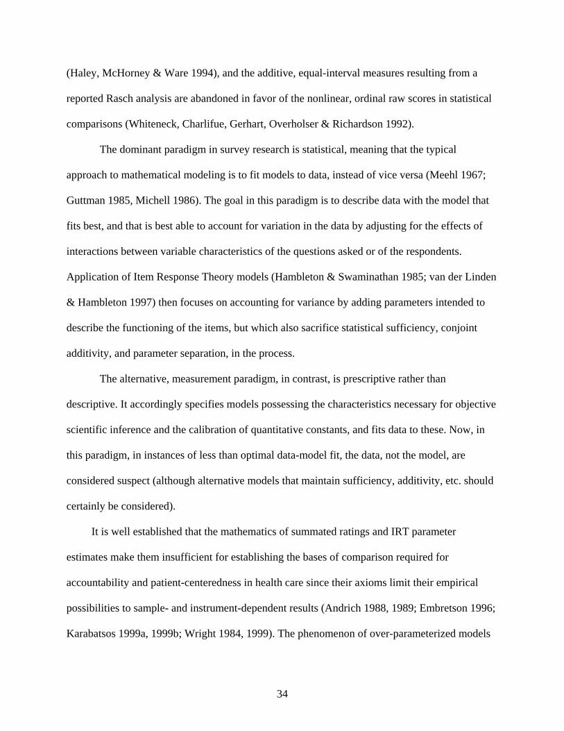
The dominant paradigm in survey research is statistical, meaning that the typical
approach to mathematical modeling is to fit models to data, instead of vice versa (Meehl 1967;
Guttman 1985, Michell 1986). The goal in this paradigm is to describe data with the model that
fits best, and that is best able to account for variation in the data by adjusting for the effects of
interactions between variable characteristics of the questions asked or of the respondents.
Application of Item Response Theory models (Hambleton & Swaminathan 1985; van der Linden
& Hambleton 1997) then focuses on accounting for variance by adding parameters intended to
describe the functioning of the items, but which also sacrifice statistical sufficiency, conjoint
additivity, and parameter separation, in the process.
The alternative, measurement paradigm, in contrast, is prescriptive rather than
descriptive. It accordingly specifies models possessing the characteristics necessary for objective
scientific inference and the calibration of quantitative constants, and fits data to these. Now, in
this paradigm, in instances of less than optimal data-model fit, the data, not the model, are
considered suspect (although alternative models that maintain sufficiency, additivity, etc. should
certainly be considered).
It is well established that the mathematics of summated ratings and IRT parameter
estimates make them insufficient for establishing the bases of comparison required for
accountability and patient-centeredness in health care since their axioms limit their empirical
possibilities to sample- and instrument-dependent results (Andrich 1988, 1989; Embretson 1996;
Karabatsos 1999a, 1999b; Wright 1984, 1999). The phenomenon of over-parameterized models
34

is not unique to IRT, but has been recognized as a problem whenever data are described so
precisely that their value as support for general conclusions is destroyed (Busemeyer & Wang
2000).
Explanations for the continued popularity of IRT and summated ratings models may also
extend beyond the logic of human sciences research methodologies to cultural assumptions about
the nature of objectivity and existence (Fisher 1992b, 1994; Michell 1990, 1999, 2000). For
instance, the IRT focus on fitting models to data may be motivated by the mistaken assumption
that it is not possible to modify scales without making new data incommensurable with old. On
the contrary, however, because PCM models are probabilistic they can account for missing data
and could play a vital role in bringing continuous quality improvement methods to bear on tests
and surveys (Wright & Stone 1979; Holm & Kavanagh 1985). This feature is in fact the basis for
recent advances in adaptive measurement and instrument equating (Lunz, Bergstrom, & Gershon
1994; Wolfe 2000). The following analyses are undertaken in the hope that some may be swayed
by empirical comparisons of the PCM and IRT methods.
Among the most well known IRT models are the 2-parameter logistic (2PL) and the 3-
parameter logistic (3PL) (Birnbaum 1968; Hambleton 1983; Hambleton & Swaminathan 1985;
Hulin, et al. 1983; Lord & Novick 1968; Lord 1980; van der Linden & Hambleton 1997).
Limiting attention to dichotomous outcomes, 2PL specifies that the probability of person n
responding positively to item i is governed by
Pr[ xni =1 | $n, *i , "i ] ≡ e["i ($n - *i )] / (ni (12)
where "i is a second item parameter denoting the discrimination index of item i, and (ni = 1 +
e["i ($n - *i )]. The inclusion of the discrimination parameter is motivated by the idea that some
35

items discriminate between lower and higher ability groups more effectively than others. 3PL
includes the pseudo-chance parameter (0i) of item i,
Pr[ xni =1 | $n, *i , "i, 0i ] ≡ 0i + (1 - 0i)[e["i ($n - *i )] / (ni] (13)
Here, 0i is an adjustment for low ability persons improbably obtaining correct responses to
difficult items.
One source of misunderstanding comes from the argument that the Rasch PCM models are
a “special case” of 2PL and 3PL models. The logic of this argument follows from the fact that,
when there are no surprising responses (0i = 0), and all items have equal discrimination ("= 1),
2PL and 3PL mathematically reduce to a Rasch PCM model. From this perspective, 2PL and
3PL are seen as offering more explanatory power than PCM models, because 2PL and 3PL do
not rest on the “restrictive” assertion that all items have the same discrimination, and that
guessing is minimal (Hambleton & Swaminathan 1985).
PCM advocates, however, show that 2PL and 3PL estimates are not based on sufficient
statistics, and that the discrimination parameter cannot be estimated independently of the person
parameter (Smith 1992; Wright 1977a, 1984, 1999). As a result, 2PL/3PL estimates will often
not converge (Stocking 1989; Hambleton & Cook 1977), which requires an upper limit to be
imposed on " (to prevent it from approaching infinity), and the assumption that $n is a normally-
distributed random variable. Furthermore, values of the discrimination parameters are
symptomatic of item bias against different examinees (Masters 1986), which means that bias can
go undetected within this framework. In addition, 2PL and 3PL demand very large samples of
persons and many test items (Hambleton 1983; Lord 1983), and even then, there is doubt as to
the accurate estimation of the pseudo-chance parameter (Hulin, et al. 1983).
36

These problems, however, are overlooked by many 2PL and 3PL practitioners. In fact, the
design of these models to fit problematic data is seen as an advantage over PCM models by IRT:
A controversial aspect of analyzing test items for model fit has always been
whether the case of a misfitting item should lead to removal of the item from the test or to a
relaxation of the model. In principle [according to IRT], both strategies are possible....a
relaxation of the Rasch [PCM] model is available in the form of the two-and three-
parameter logistic models, which may better fit problematic items (van der Linden &
Hambleton 1997, p. 12).
From the perspective of the rigorous axioms of ACM theory, however, to “relax” the
requirements of measurement to “better fit problematic items” amounts to giving up the
measurement effort. Preliminary results (Karabatsos 1999a, 1999b) show that the probability
values estimated by 2PL and 3PL cannot possibly satisfy either independence or double
cancellation, from which it follows that 2PL and 3PL cannot construct interval or ratio scale
measurement. This is because the presence of " or 0 within the models severely distorts the
scalability of persons and items. These findings confirm Cliff’s (Cliff 1992, p. 188) hypothesis:
I have argued (Cliff 1989) that the 3-PL model cannot define interval scales of
ability because the model itself contradicts the order-consistency principle [independence].
The presence of the discrimination parameter means that item difficulty order changes with
ability; the probability of a correct response is not in the same order for all persons. Thus,
order consistency is contradicted, so interval scaling is not possible. Such a difficulty does
not arise if there is only one item parameter (Roskam & Jansen 1984), leading to the Rasch
[PCM] model.
37

Furthermore, IRT models cannot provide instrument-free measurement because they incorporate
parameters, intended to describe item functioning, that “destroy the possibility of explicit
invariance of the estimates” (Andrich 1988, p. 67). Or, as another researcher (Wood 1978, p. 31)
has put it, "I am persuaded by Lumsden (Lumsden 1978) that two- and three-parameter models
are not the answer - test scaling models are self-contradictory if they assert both
unidimensionality and different slopes for the item characteristic curves,” meaning that scale-
dependencies can and do remain in data fitting IRT models with two or three item parameters.
Table 13 facilitates detailed comparison of specific features of PCM, IRT, and summated
ratings analyses as typically performed using available software.
Comparison of the PCM and IRT approaches to measurement began by attempting to
establish the extent to which 1PL IRT models produce measures equivalent to those produced by
PCM. From there, more than 25 additional IRT models involving various numbers and
combinations of item parameters, constraints, estimation methods, and MEPS item groupings
were specified and the parameters estimated. All IRT results were obtained using the
MULTILOG program (Thissen 1991). All analyses were of the 23,767 available MEPS QOC
cases, less the 208 with no data, meaning that 23,559 cases were actually in use for most
analyses.
Figure 11 shows a slightly curved, but narrow and nearly linear, relationship between
measures made using the WINSTEPS PCM software, and those made fitting a 1PL IRT model
(Samejima’s Graded Response model) using MULTILOG. For the 1PL model, discrimination
was held constant at 1.0, and the guessing parameter was not estimated. The PCM measures have
a wider distribution, and the measures are not on the identity line, but the correlation is very high
(.96).
38
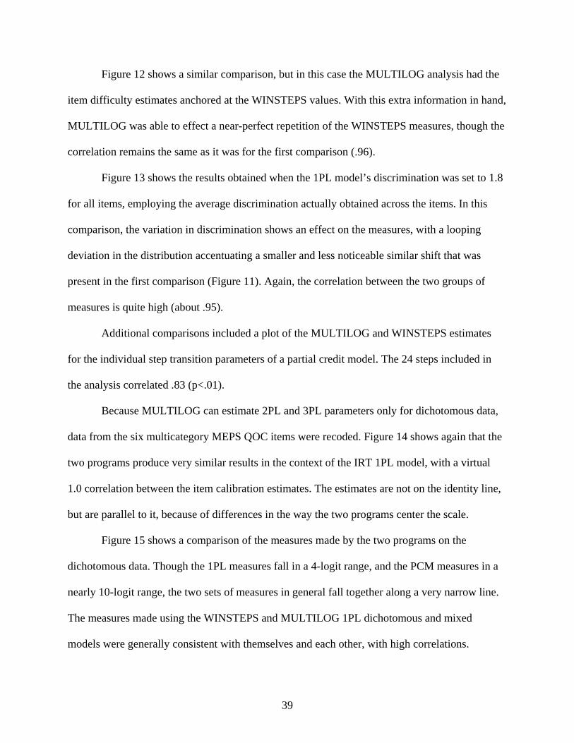
Figure 12 shows a similar comparison, but in this case the MULTILOG analysis had the
item difficulty estimates anchored at the WINSTEPS values. With this extra information in hand,
MULTILOG was able to effect a near-perfect repetition of the WINSTEPS measures, though the
correlation remains the same as it was for the first comparison (.96).
Figure 13 shows the results obtained when the 1PL model’s discrimination was set to 1.8
for all items, employing the average discrimination actually obtained across the items. In this
comparison, the variation in discrimination shows an effect on the measures, with a looping
deviation in the distribution accentuating a smaller and less noticeable similar shift that was
present in the first comparison (Figure 11). Again, the correlation between the two groups of
measures is quite high (about .95).
Additional comparisons included a plot of the MULTILOG and WINSTEPS estimates
for the individual step transition parameters of a partial credit model. The 24 steps included in
the analysis correlated .83 (p<.01).
Because MULTILOG can estimate 2PL and 3PL parameters only for dichotomous data,
data from the six multicategory MEPS QOC items were recoded. Figure 14 shows again that the
two programs produce very similar results in the context of the IRT 1PL model, with a virtual
1.0 correlation between the item calibration estimates. The estimates are not on the identity line,
but are parallel to it, because of differences in the way the two programs center the scale.
Figure 15 shows a comparison of the measures made by the two programs on the
dichotomous data. Though the 1PL measures fall in a 4-logit range, and the PCM measures in a
nearly 10-logit range, the two sets of measures in general fall together along a very narrow line.
The measures made using the WINSTEPS and MULTILOG 1PL dichotomous and mixed
models were generally consistent with themselves and each other, with high correlations.
39

Figure 16 shows the item calibrations from WINSTEPS plotted against 2PL MULTILOG
estimates. Note that the introduction of the discrimination parameter has affected the difficulty
estimates of five items in the lower left corner of the plot to the point that these five items have
nearly reversed their difficulty order. These are the five items that were originally formatted as
dichotomies. It may not be surprising to find that the discriminations for these five questions are
different from those of the rating scale items, but the question that has to be answered is whether
it is ultimately more productive to incorporate the variation in data consistency in the item
difficulty estimates, or to require a single consistency and pursue deviations from expectation by
means of residuals analyses and fit statistics.
Figure 17 shows the calibrations from WINSTEPS plotted against 3PL MULTILOG item
difficulty estimates. Allowing the difficulty estimates to be affected by unexpected extreme
responses has reversed even more the direction of the five originally dichotomous items than was
the case in the 2PL analysis.
Figure 18 shows the measures from the WINSTEPS and 2PL MULTILOG analyses. In
contrast with Figure 15’s comparisons involving the measures made using a 1PL IRT model, this
plot shows that significant additional variation in the measures has been introduced by the 2PL
discrimination parameter.
Figures 19 and 20 plot the 3PL measures against the WINSTEPS PCM and the 2PL
measures, showing that additional nonlinearities are introduced by the addition of the third item
parameter. Both figures show a floor effect evident in the 3PL measures, and Figure 20’s plot of
the 3PL and 2PL measures shows a horizontal line crossing the middle of the rest of the
distribution, apparently evidence of an inordinate adjustment made to the measures that include
the inconsistent responses to items 5 and 2, noted in the model fit analysis above.
40

The problem of knowing which item difficulty order is the right one in the context of
IRT’s multiple item parameters is aggravated by the fact that the discriminations, and so also the
item difficulty and person measurement orders, do not remain constant across models or data
input methods. Figure 21 is a plot of the discrimination values obtained for the MEPS QOC
items when different data input methods were used with the same 3PL model, and Figure 22 is a
plot of the discrimination values obtained by the 2PL and 3PL models when the same data input
method was used. In both instances, discriminations vary markedly; by necessity, so then also
will the associated item difficulty estimates vary accordingly.
RECOMMENDATIONS FOR MEPS QOC INSTRUMENT IMPROVEMENT
Instruments should be designed so as to produce internally consistent data with a high
ratio of variation to error (Fisher 2000b). In general, these features are easier to achieve if:
• the items each address a single concept, and so do not involve dependent (if-then)
clauses or conjunctions (and, or, but), since these introduce multiple concepts that cannot
later be disentangled from the data;
• the items all share a common response structure, since
o respondents can be confused by frequent changes in the available categories; and
o effective variation in the responses is easier to plan in this framework;
• the needed reliability is determined in advance, and the number of items and response
categories included in the survey are chosen so as to provide that reliability or better,
according to the well-known mathematical relationship between variation and error
(Linacre 1993); and
41

• if items are intentionally written so as to provoke even respondents with very high or
very low measures to use all of the available response options.
All of these recommendations are relevant to the measurement of QOC as achieved by the
MEPS. The MEPS has particular problems with targeting and reliability, problems that could be
effectively addressed by rethinking the questions asked in light of these analyses, analyses of
similar instruments (Fisher & Karabatsos 2000a, b; Karabatsos & Fisher 2000), and PCM theory.
DISCUSSION
Though the MEPS QOC items generally fit the PCM model, their calibrations need to
better target the sample, as is indicated in Figure 2 and by the low person separation/reliability.
This "negative" result does not mean that the measurement effort should be abandoned. Rather,
the information provided by this analysis should be used to improve the instrument. For instance,
additional difficult items, representing higher degrees of QOC, should be constructed, for the top
of the measurement range. Such items would enable the survey to better target the sample,
increasing person separation reliability and reducing opportunities for wildly inconsistent
responses by lessening the overall difference between the measures and calibrations.
The theoretically achievable reliability of .88 should be attainable with no increase in the
number of items or survey categories. All items calibrating at levels lower than one standard
deviation below the mean of the person measures should be dropped or modified such that an
equal number of items that calibrate at levels above the mean of the person measures are created.
The desired effect might be achieved simply by rephrasing existing questions or by adding more
response options, such as “Extremely Satisfied”, with the aim of making it more difficult for
respondents to employ the most positive category.
The summed ratings method fails to extract most of the relevant and useful information
available in the rating scale data. Raw scores misdirect inference on the supposition that the
42

ordinal scores can be safely treated as interval. They are also unable to tolerate missing data,
which puts out of reach practical advantages such as instrument equating, adaptive
administration, and the mediation of population-based construct differences.
The most important point relevant to the summated ratings method is that the arithmetic
logic of most statistical comparisons of sum scores requires that the intervals between rating
categories be evenly spaced. Surveys are often designed to suggest as much in the way they are
printed so as to represent the inter-category intervals as equally spaced. But the summing of
scores into a total has repeatedly been shown to be meaningful only when the numbers added up
represent something that exhibits a consistent structural magnitude (Fisher 1922; Thurstone
1926, 1928; Guttman 1985; Wilson 1971; Andersen 1977; Cliff 1982, 1989; Wright 1985, 1999;
Mundy 1986; Michell 1986, 1990, 1997, 1999; Merbitz, et al. 1989).
It may, of course, be impossible to design rating scales capable of performing so as to
exhibit the needed additive properties without additional treatments, primarily involving the
application of the natural logarithm to the distribution-free transformation of the raw scores into
odds ratios (Rasch 1960; Andersen 1977; Wright 1977b, 1985, 1999). Maor (1994) documents
the many different aspects of mathematics that the number e, on which the natural logarithm is
based, ties together: the law of compound interest in finance, the spirals of snail shells and
galaxies, equal-tempered musical scales, the area under a hyperbola, the Weber-Fechner
psychophysical law of perception, and the golden ratio exhibited in the structural proportions of
leaf patterns, the human body, and classic art. We should not be surprised to find that the number
e and the natural logarithm appear again in the structures of survey-based measurement
variables.
The comparisons of item and respondent subsample scalings reported under the headings
of hypotheses 3 and 4 present the rarely appreciated point that high reliability is not desirable for
43
purely theoretical reasons, but for the pragmatic end of providing reproducible measures. Two
instruments measuring the same thing will produce the same measure for the same amount of the
variable only within the range of error (i.e., to the extent that their measurement precision
(reliability) allows for it). When a low number of poorly designed items taken altogether
measure with a reliability below .70, as do the MEPS QOC items, and these are then divided into
two groups that measure with even lower reliabilities, low correlations (.50 - .70) between the
resulting sets of measures is to be expected.
When, in contrast, highly reliable calibrations of .94 to .96 are obtained for two different
instruments measuring the same thing, it can be expected that the measures produced will be
quite stable, and will correlate highly. The value of the Rasch separation reliability statistic
(Wright & Masters 1982) becomes apparent in this context. For a reliability of about .80 and
separation of 2.0, subsample comparison studies can be expected to produce correlations of
about .75 to .80, since, as the separation statistic indicates, the relationship of variation to error in
the measures causes the measures to vary within the bounds defined by two groups, one high and
one low. The two groups lie like oblong, slightly overlapping ellipses, end-to-end with one
another on the measurement continuum, with centers 4 errors apart. The large amount of error
relative to the variation in the measures means that treatment effects would have to be very large
to be detectable. Even in the context of relatively imprecise measurement, it remains nonetheless
true that, as long as there is more variation than error (and separation is greater than 2), measures
from different instruments experimentally established as measuring the same thing will fall
within four errors of each other more than 99% of the time.
But consider now a different situation involving two instruments addressing the same
construct, and with measurement reliabilities of .97 and separations of 6. These instruments
define six overlapping ellipses with centers 4 errors apart spread along the ruler. Just as was the
case with the lower reliability, more imprecise instruments, a measure made with one of the
44

highly precise instruments can be expected to fall within four errors of a measure of the same
amount from the other instrument better than 99% of the time. The advantage gained from the
greater precision is not only that different instruments provide more nearly the same measures
for the same amounts, but that the same numerical difference in imprecise and precise
measurement contexts will be more interpretable in the precision context, since there will be
more items articulating the substantive meaning of the score differences all along the
measurement continuum. Thus the power to make highly reliable quantitative distinctions not
only makes the detection of faint effect sizes much more likely, but it also makes them more
meaningful, since the presence of multiple items provoking the score differences provide a
language and theory of the variable.
But when results are as uncontrolled as those found in the application of the
multiparameter IRT models, where are criteria for knowing which difficulty order is right to
come from? The only place they can come from is from the identification of constant, additive
relationships capable of supporting generalizable comparisons. In actual practice, multiparameter
IRT estimation procedures require the estimation of a PCM model every other iteration in order
to prevent the estimates from diverging to infinity (Stocking 1989). And when instruments have
to be equated so that measures can be compared, it is again PCM, in effect, that is put to use,
since the need for stable estimates across samples is the well-accepted point of equating. If we
are then to engineer quantitative measures of QOC, functional status, quality of life, or other
variables that effect what Roche (1998) calls the full integration of measurement and
mathematics in scale-free metrics, there would seem to be no point in employing analytic
methods and theories like IRT and summated ratings that do not efficiently facilitate the
realization of that goal.
45

Both the history of measurement science (Heilbron 1993, Roche 1998) and
developmental psychology (Bergling 1999; Dawson 2000) show that understanding evolves over
time through interaction with objects. Interactions with the things themselves provoke qualitative
cognitive and social shifts in understanding and behavior. Given acceptance of the criteria for
fundamental measurement essential to science and commerce, the hypothesis that PCM, IRT,
and summated ratings approaches each have an appropriate place in QOC measurement could be
accepted, with qualifications, in the framework of an evolutionary perspective.
A paradigm shift similar to the one that provoked what Kuhn (1961) calls the “second
scientific revolution” in the 19th Century may be occurring in the world of measurement methods
based in tests and surveys. For instance, even though raw scores are nearly linear in the presence
of complete data and in the middle of the score distribution, PCM makes it possible to obtain
linear measures in the presence of missing data and across the entire range of the distribution.
Even though measurement via tests and surveys seems to have functioned well enough without
tests of the quantitative hypothesis, and without routine data quality assessment, perhaps
demands for accountability will make those omissions less tolerable. And even though scale-
dependent metrics may not have seemed terribly cumbersome over the course of the 20th
Century, in the context of the 21st Century’s ubiquitous computer networks and streamlined
communications, scale-free metrics will soon become the new norm.
Similarly, even though the 1 PL IRT measures and calibrations are statistically identical
with the PCM measures and calibrations, the IRT analysis does nothing to test Hypothesis 1,
above, that the QOC variable is quantitative, since no data-model fit tests of independence and
double cancellation are provided. It is also true that, in the contexts of the 2PL and 3PL models,
as shown below, tests of Hypothesis 1 would be inconsistent with the mathematics structuring
the estimation process, since the tests would be checking for the invariance that the models
46

overtly compromise by shifting the item difficulty order according to the discriminatory power
of each individual item. IRT criteria for model choice are accordingly based in the statistical
capacity of the models to account for variation in the data. When applied to the MEPS QOC
data, the 3PL and 2PL IRT models clearly fit better than the 1PL model did, with respective chi-
square statistics of -293,899, -293,209, and -288,498.
These statistical results are confounded, however, by the plots clearly showing that the
ordering and meaning of the measures and calibrations produced by the 2PL and 3PL IRT
models vary in arbitrary and uninterpretable ways. Rather than implementing the long-proven
methods of science that value measurement for revealing anomalous failures of invariance, and
so facilitating data quality assessment and the identification of new constructs requiring
investigation (Kruskal 1960; Kuhn 1961, Wimsatt 1981), IRT integrates anomalous interactions
into the measures and calibrations, concealing unexpected observations deep within the results
and destroying the possibility of quantitative comparability (Embretson 1996).
The IRT analysis also falls short of the PCM standard in not providing the graphic
displays of the construct needed for assessing the interpretability of the measures and
calibrations.
Referring again to those displays, in Figures 2 and 3, the overall MEPS QOC item order
indicates that matters of access to care are of more concern to respondents than matters
pertaining to the provider. Though not yet widely recognized, a general pattern in QOC and
satisfaction with health care services has been observed across several independent studies
(Angelico & Fisher 2000a, 2000b; Fisher 1992a; Fisher & Karabatsos 2000a, 2000b; Karabatsos
& Fisher 2000). This pattern indicates that 1) the highest quality of care or satisfaction with
services is usually associated with the physician; 2) somewhat less quality is associated with
nursing, allied health staff, and general access to care; 3) less quality yet is found with regard to
47

office staff, making appointments, and telephone access; and 4) the least quality is associated
with waiting room comfort and cleanliness, and parking availability.
Plainly, the existence of this continuum does not imply that waiting room comfort and
cleanliness ought to be improved so as to provoke ratings equivalent to those obtained by the
physician. On the contrary, in the spirit of continuous quality assessment and improvement
(McLaughlin & Kaluzny 1999), the theoretical stability of the QOC continuum across
instruments, providers, and health care consumers ought to be employed as the criterion
reference against which quality improvement efforts are evaluated. Instead of adopting the
quality control approach’s futile efforts to cut off the low quality tail of the measurement
distribution, the point is instead to move the entire distribution up the ruler to an overall higher
quality.
Should this as yet informally documented pattern prove to be stable across brands of
instruments, as has been found to be the case with clinician-assigned ratings of physical
functioning (Fisher 1997a, 1997b; Fisher, Harvey, Taylor, et al. 1995), it should be possible to
calibrate a reference standard metric to which all instruments measuring QOC would be
traceable, using methods adapted from the existing standard procedures of metrology (Mandel
1977 1978; Wernimont 1977, 1978; Pennella 1997).
CONCLUSION
Although the MEPS QOC instrument will need certain refinements to optimize its
functioning, PCM analysis provides clear evidence that fundamental measurement systems can
be created for QOC variables.
Given a sufficiently reliable QOC measurement system, it should be possible to equate
different QOC measures together so as to make them traceable to a reference standard metric.
Fisher and Karabatsos (2003) compare PCM analyses of the MEPS QOC items with similar
48

analyses of the QOC-specific items from the Consumer Assessment of Health Plans Study
(CAHPS, version 2.0 Adult Core items), also funded by AHRQ. Given that there are no items
common to both the MEPS and the CAHPS, and that the MEPS measurement reliability is so
low, equating would probably not be viable. As an alternative, a new instrument has been
designed according to the PCM principles described above and following the content included in
the MEPS and CAHPS QOC scales. Research on this scale continues.
In practice, much research presented in the context of IRT, Rasch measurement, latent
trait theory, or conjoint analysis is, or strives, in effect, to be PCM. But the hypotheses tested in
these reports vary widely, as does the quality of their execution. The present report itself is
undoubtedly far from perfect, but it is hoped that it may be taken as a contribution toward the
development of improved research standards in the human sciences.
49

References Cited Andersen, E. B. (1977). Sufficient statistics and latent trait models. Psychometrika, 42(1), 69-81. Andrich, D. (1988). Sage University Paper Series on Quantitative Applications in the Social Sciences. Vol. series no. 07-068: Rasch models for measurement. Beverly Hills, California: Sage Publications.
Andrich, D. (1989). Distinctions between assumptions and requirements in measurement in the social sciences. In J. A. Keats, R. Taft, R. A. Heath & S. H. Lovibond (Eds.), Mathematical and Theoretical Systems: Proceedings of the 24th International Congress of Psychology of the International Union of Psychological Science, Vol. 4 (pp. 7-16). North-Holland: Elsevier Science Publishers.
Angelico, D., Fisher, W. P., Jr. (2000a). Measuring patient satisfaction in the LSU Health Care Services Division. International Objective Measurement Workshops, New Orleans, April.
Angelico, D., Fisher, W. P., Jr. (2000b). Reliability in the measurement of patient satisfaction. Sixth AHRQ/CDC Building Bridges Conference. Atlanta, April. Bergling, B. M. (1999, Sep). Developmental changes in reasoning strategies: Equating scales for two age groups. European Psychologist, 4(3), 157-164.
Bernhard, J., Cella, D. F., Coates, A. S., Fallowfield, L., Ganz, P. A., Moinpour, C. M., Mosconi, P., Osoba, D., Simes, J., & Hurny, C. (1998, Mar). Missing quality of life data in cancer clinical trials: Serious problems and challenges. [Review] [42 refs]. Statistics in Medicine, 17(5-7), 15-Apr. Birnbaum, A. (1968). Some latent trait models and their use in inferring an examinee's ability. In F. M. Lord & M. R. Novick (Eds.), Statistical theories of mental test scores. Reading, Massachusetts: Addison-Wesley. Brogden, H. E. (1977). The Rasch model, the law of comparative judgment and additive conjoint measurement. Psychometrika, 42, 631-634.
Busemeyer, J. R., & Wang, Y.-M. (2000, March). Model comparisons and model selections based on generalization criterion methodology. Journal of Mathematical Psychology, pp. 171-189. Cherryholmes, C. (1988). Construct validity and the discourses of research. American Journal of Education, 96(3), 421-457. Cliff, N. (1982). What is and isn't measurement. In G. Keren (Ed.), Statistical and methodological issues in psychology and social sciences research (pp. 3-38). Hillsdale, New Jersey: Lawrence Erlbaum Associates. Cliff, N. (1989). Ordinal consistency and ordinal true scores. Psychometrika, 54, 75-91. Cliff, N. (1992). Abstract measurement theory and the revolution that never happened. Psychological Science, 3, 186-190. Cohen, J., Monheit, A. C., Beauregard, K. M., Cohen, S., Lefkowitz, D., Potter, D., Sommers, J., Taylor, A., & Arnett, R. (1996-97, Winter). The Medical Expenditure Panel Survey: A national health information resource. Inquiry, 33(4), 373-89. Connolly, A. J., Nachtman, W., & Pritchett, E. M. (1971). Keymath: Diagnostic Arithmetic Test. Circle Pines, MN: American Guidance Service. Dawson, T. L. (2000). Moral and evaluative reasoning across the life-span. Journal of Applied Measurement, 1(4), 346-371.
50

Duncan, O. D. (1984). Notes on social measurement: Historical and critical. New York: Russell Sage Foundation. Embretson, S. E. (1996, September). Item Response Theory models and spurious interaction effects in factorial ANOVA designs. Applied Psychological Measurement, 20(3), 201-212. Falmagne, J.-C. (1979). On a class of probabilistic conjoint measurement models: Some diagnostic properties. Journal of Mathematical Psychology, 19, 73-88. Fisher, R. A. (1922). On the mathematical foundations of theoretical statistics. Philosophical Transactions of the Royal Society of London, A, 222, 309-368.
Fisher, W. P., Jr. (1992a). Measuring rehabilitation client satisfaction. Midwest Objective Measurement Seminar, University of Chicago, December.
Fisher, W. P., Jr. (1992b). Objectivity in measurement: A philosophical history of Rasch's separability theorem. In M. Wilson (Ed.), Objective measurement: Theory into practice. Vol. I (pp. 29-58). Norwood, New Jersey: Ablex Publishing Corporation. Fisher, W. P., Jr. (1993, April). Measurement-related problems in functional assessment. The American Journal of Occupational Therapy, 47(4), 331-338. Fisher, W. P., Jr. (1994). The Rasch debate: Validity and revolution in educational measurement. In M. Wilson (Ed.), Objective measurement: Theory into practice. Vol. II (pp. 36-72). Norwood, New Jersey: Ablex Publishing Corporation. Fisher, W. P., Jr. (1997a). Physical disability construct convergence across instruments: Towards a universal metric. Journal of Outcome Measurement, 1(2), 87-113. Fisher, W. P., Jr. (1997b, June). What scale-free measurement means to health outcomes research. Physical Medicine & Rehabilitation State of the Art Reviews, 11(2), 357-373. Fisher, W. P., Jr. (1998). A research program for accountable and patient-centered health status measures. Journal of Outcome Measurement, 2(3), 222-239. Fisher, W. P., Jr. (2000a). Objectivity in psychosocial measurement: What, why, how. Journal of Outcome Measurement, 4(2), 527-563.
Fisher, W. P., Jr. (2000b). Survey design recommendations. Popular Measurement, 3(1), 58-9. Fisher, W. P., Jr., Harvey, R. F., & Kilgore, K. M. (1995). New developments in functional assessment: Probabilistic models for gold standards. NeuroRehabilitation, 5(1), 3-25.
Fisher, W. P., Jr., Harvey, R. F., Taylor, P., Kilgore, K. M., & Kelly, C. K. (1995). Rehabits: A common language of functional assessment. Archives of Physical Medicine and Rehabilitation, 76, 113-122.
Fisher, William P., Karabatsos, G. (2000a). Fundamental measurement with MEPS/CAHPS quality of care data. Presented at the Third International Outcome Measurement Conference. Northwestern Memorial Hospital, Chicago, June.
Fisher, W. P., Jr., Karabatsos, G. (2000b). Quality of care metrology: New possibilities for generalized quantification. American Public Health Association, Boston, November. Goldstein, H. (1979). Consequences of using the Rasch model for educational assessment. British Educational Research Journal, 5(2), 211-220. Goldstein, H., & Blinkhorn, S. (1977). Monitoring educational standards -- An inappropriate model. Bulletin of the British Psychological Society, 30, 309-311. Green, S. B., Lissitz, R. W., & Mulaik, S. A. (1977, Winter). Limitations of coefficient alpha as an index of test unidimensionality. Educational and Psychological Measurement, 37(4), 827-833.
51

Gustafsson, J.-E. (1980). Testing and obtaining fit of data to the Rasch model. British Journal of Mathematical and Statistical Psychology, 33, 205-233. Guttman, L. (1985). The illogic of statistical inference for cumulative science. Applied Stochastic Models and Data Analysis, 1, 3-10. Hahn, E., Webster, K. A., Cella, D., & Fairclough, D. (1998, Mar). Missing data in quality of life research in Eastern Cooperative Oncology Group (ECOG) clinical trials: Problems and solutions. Statistics in Medicine, 17(5-7), 15-Apr. Haley, S. M., McHorney, C. A., & Ware, J. E., Jr. (1994). Evaluation of the MOS SF-36 physical functioning scale (PF-10): I. unidimensionality and reproducibility of the Rasch item scale. Journal of Clinical Epidemiology, 47(6), 671-684. Hambleton, R. (Editor). (1983). Applications of Item Response Theory (IRT). Vancouver, BC: Educational Research Institute of British Columbia. Hambleton, R. K., & Cook, L. L. (1977). Latent trait models and their use in the analysis of educational test data. Journal of Educational Measurement, 14(2), 75-96. Hambleton, R. K., & Swaminathan, H. (1985). Item response theory: Principles and applications. Hingham, MA: Kluwer. Heilbron, J. L. (1993). Weighing imponderables and other quantitative science around 1800. Historical studies in the physical and biological sciences (Vol. 24 (Supplement), Part I, pp. 1-337). Berkeley, California: University of California Press.
Holm, K., & Kavanagh, J. (1985). An approach to modifying self-report instruments. Research in Nursing and Health, 8, 13-18. Hulin, C. L., Drasgow, F., & Parsons, C. K. (1983). Item response theory: Applications to psychological measurement. Homewood: Dow Jones Irwin.
Karabatsos, G. (1999a, April). Rasch versus 2PL/3PL in axiomatic measurement theory. In Session 53.50, K. F. Cook (Chair), Theoretical issues in Rasch measurement. American Educational Research Association. Montreal, Canada: Rasch Measurement SIG. Karabatsos, G. (1999b). Representational measurement theory as a basis for model selection in item-response theory. Society of Mathematical Psychology. Santa Cruz, CA.
Karabatsos, G., Fisher, W. P., Jr. (2000). MEPS and CAHPS quality of care calibration results. American Public Health Association, Boston, November. Kolen, M. J., & Brennan, R. L. (1995). Test equating. New York: Springer. Krantz, D. H., Luce, R. D., Suppes, P., & Tversky, A. (1971). Foundations of measurement. Volume 1: Additive and polynomial representations. New York, New York: Academic Press. Kruskal, W. H. (1960). Some remarks on wild observations. Technometrics, 2, 1-3. (Rpt. in H. H. Ku, (Ed.). (1969). Precision measurement and calibration (pp. 346-8). Washington, DC: National Bureau of Standards). Kuhn, T. S. (1961). The function of measurement in modern physical science. Isis, 52(168), 161-193. (Rpt. in The essential tension: Selected studies in scientific tradition and change (pp. 178-224). Chicago, Illinois: University of Chicago Press). Likert, R. (1932). A technique for the measurement of attitudes. Archives of Psychology, 140, 5-55. Linacre, J. M. (1993). Rasch generalizability theory. Rasch Measurement Transactions, 7(1), 283-284; Linacre, J. M. (1997). Instantaneous measurement and diagnosis. Physical Medicine and Rehabilitation State of the Art Reviews, 11(2), 315-324.
52

Linacre, J. M. (1998). Detecting multidimensionality: Which residual data-type works best? Journal of Outcome Measurement, 2(3), 266-83. Linacre, J. M. (1999). Investigating rating scale category utility. Journal of Outcome Measurement, 3(2), 103-22. Lord, F. M. (1980). Applications of item response theory to practical testing problems. Hillsdale, New Jersey: Lawrence Erlbaum. Lord, F. M. (1983). Small N justifies Rasch model. In D. J. Weiss (Ed.), New horizons in testing: Latent trait test theory and computerized adaptive testing (pp. 51-61). New York, New York: Academic Press, Inc. Lord, F. M., & Novick, M. R. (Eds.). (1968). Statistical theories of mental test scores. Reading, Massachusetts: Addison-Wesley. Luce, R. D., & Tukey, J. W. (1964). Simultaneous conjoint measurement: A new kind of fundamental measurement. Journal of Mathematical Psychology, 1(1), 1-27. Ludlow, L. H., & Haley, S. M. (1995, December). Rasch model logits: Interpretation, use, and transformation. Educational and Psychological Measurement, 55(6), 967-975. Ludlow, L. H., & Haley, S. M. (1992). Polytomous Rasch models for behavioral assessment: The Tufts Assessment of Motor Performance. In M. Wilson (Ed.), Objective measurement: Theory into practice, Volume 1 (pp. 121-137). Norwood, New Jersey: Ablex Publishing Corporation. Lumsden, J. (1978). Tests are perfectly reliable. British Journal of Mathematical and Statistical Psychology, 31, 19-26. Lunz, M. E., Bergstrom, B. A., & Gershon, R. C. (1994). Computer adaptive testing. International Journal of Educational Research, 21(6), 623-634. Maor, E. (1994). e: The story of a number. Princeton, New Jersey: Princeton University Press. Mandel, J. (1977, March). The analysis of interlaboratory test data. ASTM Standardization News, 5, 17-20, 56. Mandel, J. (1978, December). Interlaboratory testing. ASTM Standardization News, 6, 11-12. Masters, G. N. (1986). Item discrimination: When more is worse. Journal of Educational Measurement, 24, 15-29. McDowell, I., & Newell, C. (1996). Measuring health: A guide to rating scales and questionnaires. 2d edition. Oxford: Oxford University Press. McHorney, C. A. (1997, Oct 15). Generic health measurement: Past accomplishments and a measurement paradigm for the 21st century. [Review] [102 refs]. Annals of Internal Medicine, 127(8 Pt 2), 743-50. McLaughlin, C. P., & Kaluzny, A. D. (1999). Continuous quality improvement in health care: Theory, implementation, and applications. Gaithersburg, Maryland: Aspen Publishers, Inc.
Meehl, P. E. (1967). Theory-testing in psychology and physics: A methodological paradox. Philosophy of Science, 34(2), 103-115. Merbitz, C., Morris, J., & Grip, J. (1989). Ordinal scales and the foundations of misinference. Archives of Physical Medicine and Rehabilitation, 70, 308-312. Messick, S. (1975, October). The standard problem: Meaning and values in measurement and evaluation. American Psychologist, 30, 955-966. Michell, J. (1986). Measurement scales and statistics: A clash of paradigms. Psychological Bulletin, 100, 398-407.
53

Michell, J. (1990). An introduction to the logic of psychological measurement. Hillsdale, New Jersey: Lawrence Erlbaum Associates. Michell, J. (1997). Quantitative science and the definition of measurement in psychology. British Journal of Psychology, 88, 355-383. Michell, J. (1999). Measurement in psychology: A critical history of a methodological concept. Cambridge: Cambridge University Press. Michell, J. (2000, October). Normal science, pathological science and psychometrics. Theory & Psychology, 10(5), 639-667. Mundy, B. (1986). On the general theory of meaningful representation. Synthese, 67, 391-437. Ottenbacher, K. J., & Tomchek, S. D. (1993). Measurement in rehabilitation research: Consistency versus consensus. Physical Medicine and Rehabilitation Clinics of North America, 4(3), 463-473. Pennella, C. R. (1997). Managing the metrology system. Milwaukee, WI: ASQ Quality Press. Perline, R., Wright, B. D., & Wainer, H. (1979). The Rasch model as additive conjoint measurement. Applied Psychological Measurement, 3(2), 237-255. Phillips, S. E. (1986). The effects of the deletion of misfitting persons on vertical equating via the Rasch model. Journal of Educational Measurement, 23(2), 107-118. Rasch, G. (1960). Probabilistic models for some intelligence and attainment tests (reprint, with Foreword and Afterword by B. D. Wright, Chicago: University of Chicago Press, 1980). Copenhagen, Denmark: Danmarks Paedogogiske Institut. Revicki, D. A., & Cella, D. F. (1997, Aug). Health status assessment for the twenty-first century: Item response theory item banking and computer adaptive testing. Quality of Life Research, 6(6), 595-600. Roche, J. (1998). The mathematics of measurement: A critical history. London: The Athlone Press. Roskam, E. E., & Jansen, P. G. W. (1984). A new derivation of the Rasch model. In E. DeGreef & J. van Buggenhaut (Eds.), Trends in mathematical psychology. Amsterdam: Elsevier. Scott, D., & Suppes, P. (1958, June). Foundational aspects of theories of measurement. The Journal of Symbolic Logic, 23(2), 113-128. Smith, R. M. (1986). Person fit in the Rasch model. Educational and Psychological Measurement, 46, 359-372. Smith, R. M. (1988). The distributional properties of Rasch standardized residuals. Educational & Psychological Measurement, 48(3), 657-667. Smith, R. M. (1991). The distributional properties of Rasch item fit statistics. Educational and Psychological Measurement, 51, 541-565.
Smith, R. M. (1992). Applications of Rasch measurement. Chicago, Illinois: MESA Press. Smith, R. M., Schumacker, R. E., & Bush, M. J. (1998). Using item mean squares to evaluate fit to the Rasch model. Journal of Outcome Measurement, 2(1), 66-78. Sparrow, S., Balla, D., & Cicchetti, D. (1984). Interview edition, survey form manual, Vineland Behavior Scales. Circle Pines, MN: American Guidance Services, Inc. Streiner, D. L., & Norman, G. R. (1995). Health measurement scales: A practical guide to their development and use, 2d edition. New York, New York: Oxford University Press.
54

Stucki, G., Daltroy, L., Katz, N., Johannesson, M., & Liang, M. H. (1996). Interpretation of change scores in ordinal clinical scales and health status measures: The whole may not equal the sum of the parts. Journal of Clinical Epidemiology, 49(7), 711-717. Suppes, P., Krantz, D., Luce, R. D., & Tversky, A. (1989). Foundations of measurement, Volume II: Geometric and probabilistic representations. New York: Academic Press.
Thissen, D. (1991). MULTILOG, V. 6. Chicago, Illinois: Scientific Software, Inc. Thurstone, L. L. (1926). The scoring of individual performance. Journal of Educational Psychology, 17, 446-457.
Thurstone, L. L. (1928). Attitudes can be measured. American Journal of Sociology, XXXIII, 529-544. Reprinted in L. L. Thurstone, The Measurement of Values. Midway Reprint Series. Chicago, Illinois: University of Chicago Press, 1959, pp. 215-233. Troxel, A. B., Fairclough, D. L., Curran, D., & Hahn, E. (1998). Statistical analysis of quality of life with missing data in cancer clinical trials: Problems and solutions. Statistics in Medicine, 17, 547-59. van der Linden, W. J., & Hambleton, R. K. (1997). Item response theory: A brief history. Handbook of Modern Item Response Theory (IRT)W. J. van der Linden & R. K. Hambleton (Eds.), (pp. 1-28). New York: Springer-Verlag. Wernimont, G. (1977, March). Ruggedness evaluation of test procedures. ASTM Standardization News, 5, 13-16. Wernimont, G. (1978, December). Careful intralaboratory study must come first. ASTM Standardization News, 6, 11-12. Whiteneck, G. G., Charlifue, S. W., Gerhart, K. A., Overholser, J. D., & Richardson, G. N. (1992, June). Quantifying handicap: A new measure of long-term rehabilitation outcomes. Archives of Physical Medicine and Rehabilitation, 73(6), 519-526. Wilson, T. P. (1971). Critique of ordinal variables. Social Forces, 49, 432-444. Wimsatt, W. C. (1981). Robustness, reliability and overdetermination. In M. B. Brewer & B. E. Collins (Eds.), Scientific inquiry and the social sciences. San Francisco: Jossey-Bass. Wolfe, E. W. (2000). Equating and item banking with the Rasch model. Journal of Applied Measurement, 1(4), 409-434. Wood, R. (1978). Fitting the Rasch model: A heady tale. British Journal of Mathematical and Statistical Psychology, 31, 27-32. Woodcock, R. W. (1973). Woodcock Reading Mastery Tests. Circle Pines, MN: American Guidance Service, Inc. Woodcock, R. W. (1999). What can Rasch-based scores convey about a person's test performance? In S. E. Embretson & S. L. Hershberger (Eds.), The new rules of measurement: What every psychologist and educator should know. Hillsdale, NJ: Lawrence Erlbaum Associates.
Wright, B. D. (1977a). Misunderstanding the Rasch model. Journal of Educational Measurement, 14(3), 219-225. Wright, B. D. (1977b). Solving measurement problems with the Rasch model. Journal of Educational Measurement, 14(2), 97-116. Wright, B. D. (1984). Despair and hope for educational measurement. Contemporary Education Review, 3(1), 281-288. Wright, B. D. (1985). Additivity in psychological measurement. In E. Roskam (Ed.), Measurement and personality assessment. North Holland: Elsevier Science Ltd.
55

Wright, B. D. (1999). Fundamental measurement for psychology. In S. E. Embretson & S. L. Hershberger (Eds.), The new rules of measurement: What every educator and psychologist should know. Hillsdale, NJ: Lawrence Erlbaum Associates. Wright, B. D., & Linacre, J. M. (1989). Observations are always ordinal; measurements, however, must be interval. Archives of Physical Medicine and Rehabilitation, 70(12), 857-867. Wright, B. D., & Linacre, J. M. (1999). A User's Guide to WINSTEPS Rasch-Model Computer Program, v. 2.94. Chicago: MESA Press. Wright, B. D., & Masters, G. N. (1982). Rating scale analysis: Rasch measurement. Chicago: MESA Press. Wright, B. D., & Stone, M. H. (1979). Best test design: Rasch measurement. Chicago: MESA Press. Zhu, W. (1996). Should total scores from a rating scale be used directly? Research Quarterly for Exercise and Sport, 67(3), 363-372.
56

ITEMS Person v w y z Score (1a) βn P a 1 1 1 0 3 1.1 E b 1 1 1 0 3 1.1 R c 1 0 1 0 2 0 S d 1 1 0 0 2 0 O e 1 0 0 0 1 -1.1 N f 0 0 0 1 1 -1.1 S Item Score (1b) 5 3 3 1 δi -1.6 0 0 1.6
Table 1. Six persons’ responses to a 4-item survey.
57

ITEMS v w y z βn P a .94 .75 .75 .38 1.1 E b .94 .75 .75 .38 1.1 R c .83 .50 .50 .17 0 S d .83 .50 .50 .17 0 O e .63 .25 .25 .06 -1.1 N f .63 .25 .25 .06 -1.1 δi -1.6 0 0 1.6
Table 2. The data in Table 1 expressed as probabilities.
58

_____________________________________________________________________
Person Summary (N=20,011)
Measure Error IMS OMS
Mean 2.08 .85 .93 .88
S.D. 1.42 .37 .74 1.10
Min. -2.95 .43 .00 .00
Max. 5.04 4.07 5.60 9.9
ASD = 1.08 RMSE = .92
Separation = 1.17 Real Reliability = .58
(Model Reliability = .65)
Item Summary (I=11)
Measure Error IMS OMS
0.00 .02 .99 .93
1.02 .01 .14 .29
-1.49 .01 .79 .44
1.59 .04 1.28 1.55
ASD = .02 RMSE = 1.02
Separation = 51 Real Reliability = 1.0
_____________________________________________________________________
Table 3. Summary statistics for measures and MEPS QOC items.
59
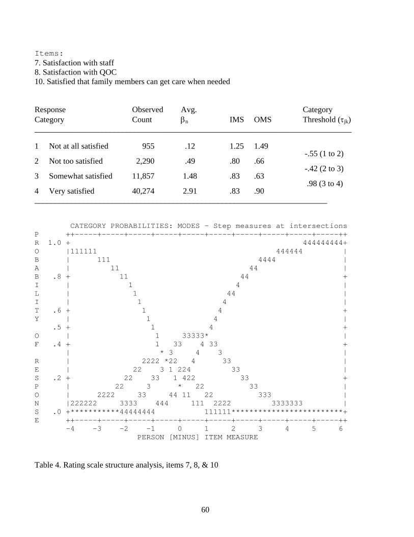
Items: 7. Satisfaction with staff 8. Satisfaction with QOC 10. Satisfied that family members can get care when needed
Response Observed Avg. Category Category Count βn IMS OMS Threshold (τjk) ______________________________________________________________________________
1 Not at all satisfied 955 .12 1.25 1.49 -.55 (1 to 2)
2 Not too satisfied 2,290 .49 .80 .66 -.42 (2 to 3)
3 Somewhat satisfied 11,857 1.48 .83 .63 .98 (3 to 4)
4 Very satisfied 40,274 2.91 .83 .90 ________________________________________________________________________
CATEGORY PROBABILITIES: MODES - Step measures at intersections P ++-----+-----+-----+-----+-----+-----+-----+-----+-----+-----++ R 1.0 + 444444444+ O |111111 444444 | B | 111 4444 | A | 11 44 | B .8 + 11 44 + I | 1 4 | L | 1 44 | I | 1 4 | T .6 + 1 4 + Y | 1 4 | .5 + 1 4 + O | 1 33333* | F .4 + 1 33 4 33 + | * 3 4 3 | R | 2222 *22 4 33 | E | 22 3 1 224 33 | S .2 + 22 33 1 422 33 + P | 22 3 * 22 33 | O | 2222 33 44 11 22 333 | N |222222 3333 444 111 2222 3333333 | S .0 +***********44444444 111111*************************+ E ++-----+-----+-----+-----+-----+-----+-----+-----+-----+-----++ -4 -3 -2 -1 0 1 2 3 4 5 6 PERSON [MINUS] ITEM MEASURE
Table 4. Rating scale structure analysis, items 7, 8, & 10
60
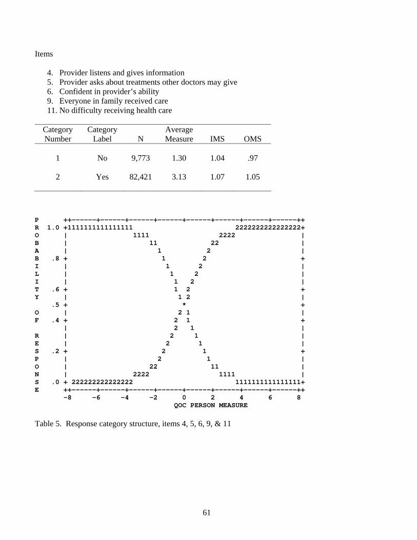
Items
4. Provider listens and gives information 5. Provider asks about treatments other doctors may give 6. Confident in provider’s ability 9. Everyone in family received care 11. No difficulty receiving health care
Category Number
Category Label
N
Average Measure
IMS
OMS
1
No
9,773
1.30
1.04
.97
2
Yes
82,421
3.13
1.07
1.05
P ++------+------+------+------+------+------+------+------++ R 1.0 +1111111111111111 2222222222222222+ O | 1111 2222 | B | 11 22 | A | 1 2 | B .8 + 1 2 + I | 1 2 | L | 1 2 | I | 1 2 | T .6 + 1 2 + Y | 1 2 | .5 + * + O | 2 1 | F .4 + 2 1 + | 2 1 | R | 2 1 | E | 2 1 | S .2 + 2 1 + P | 2 1 | O | 22 11 | N | 2222 1111 | S .0 + 222222222222222 1111111111111111+ E ++------+------+------+------+------+------+------+------++ -8 -6 -4 -2 0 2 4 6 8
QOC PERSON MEASURE Table 5. Response category structure, items 4, 5, 6, 9, & 11
61

Items 1. How difficult is it to get appointments? 3. How difficult is it to contact provider by phone?
Category Number
Category Label
N
Average Measure
IMS
OMS
Step Threshold
1
Very
Difficult
2,989
−0.59
.95
.91
2
Somewhat Difficult
4,892
0.07
.94
.84
3
Not Too Difficult
11,630
0.82
.93
.80
4
Not at all Difficult
13,390
1.90
1.16
1.11
−0.72 (1→2) −0.43 (2→3) 1.16 (3→4)
CATEGORY PROBABILITIES: MODES - Step measures at intersections P ++-----+-----+-----+-----+-----+-----+-----+-----+-----+-----++ R 1.0 + 44444444+ O |11111 444444 | B | 111 4444 | A | 11 44 | B .8 + 11 44 + I | 1 4 | L | 1 44 | I | 1 4 | T .6 + 1 4 + Y | 1 4 | .5 + 1 3333 4 + O | 1 33 3* | F .4 + 1 3 4 33 + | 22*2* 4 3 | R | 222 *3 22 4 33 | E | 22 3 1 2 4 33 | S .2 + 22 3 11 *2 33 + P | 22 3 *4 22 33 | O | 2222 333 44 11 22 3333 | N |22222 333 444 111 22222 333333 | S .0 +***********44444444 1111111************************+ E ++-----+-----+-----+-----+-----+-----+-----+-----+-----+-----++ -4 -3 -2 -1 0 1 2 3 4 5 6 PERSON [MINUS] ITEM MEASURE Table 6. Response category structure, items 1 & 3
62

Item 2. How long is the usual wait for a medical appointment?
Category Number
Category Label
N
Average Measure
IMS
OMS
Step Threshold
1
>2 hours
250
0.38
1.37
1.44
2
1-2 hours
1,111
0.89
1.24
1.29
3
31 to 59 minutes
1,831
1.34
1.17
1.20
4
16 to 30 minutes
5,212
1.95
1.21
1.20
2.69 (1→2) 1.11 (2→3) 1.06 (3→4) 0.43 (4→5)
5
5-15
minutes
7,387
2.92
1.24
1.16
4.43 (5→6)
6 <5 minutes
669 3.33 1.82 1.26
CATEGORY PROBABILITIES: MODES - Step measures at intersections P ++-----+-----+-----+-----+-----+-----+-----+-----+-----+-----++ R 1.0 + + O | | B | | A | 6| B .8 +1 5555 6 + I | 1 555 555 66 | L | 1 5 55 66 | I | 11 55 55 6 | T .6 + 1 5 5 6 + Y | 1 5 5 6 | .5 + 1 222 5 5* + O | *2 22 444444* 66 5 | F .4 + 22 1 2 4 5 4 6 5 + | 22 1 2 4 5 44 6 5 | R | 2 1 3**3 5 4 6 55 | E | 22 1 33 42 33 5 44 66 5 | S .2 +2 3* 4 2 *3 44 66 55 + P | 33 *4 ** 33 44 66 5| O | 333 44 11 5 22 33 6**4 | N | 3333 444 55**1 222 333366666 444444 | S .0 +***************66666*****************************************+ E ++-----+-----+-----+-----+-----+-----+-----+-----+-----+-----++ -4 -3 -2 -1 0 1 2 3 4 5 6 PERSON [MINUS] ITEM MEASURE Table 7. Response category structure, item 2
63

ITEMS LOWDIF MIDDIFF HIDIFF43,44,47,49,
51,5242,45,46,48,
50LOWDIFF Pearson
Correlation1.000 .718 .255 .706 .524
Sig. (2-tailed)
. .000 .000 .000 .000
N 16121 16069 11476 16121 16121MIDDIFF Pearson
Correlation.718 1.000 .470 .875 .680
Sig. (2-tailed)
.000 . .000 .000 .000
N 16069 16083 11476 16069 16069HIDIFF Pearson
Correlation.255 .470 1.000 .889 .799
Sig. (2-tailed)
.000 .000 . .000 .000
N 11476 11476 11476 11476 11476RandomSelection
43,44,47,49,51,52
Pearson Correlation
.706 .875 .889 1.000 .813
Sig. (2-tailed)
.000 .000 .000 . .000
N 16121 16069 11476 16121 16121RandomSelection
42,45,46,48,50
Pearson Correlation
.524 .680 .799 .813 1.000
Sig. (2-tailed)
.000 .000 .000 .000 .
N 16121 16069 11476 16121 16121** Correlation is significant at the 0.01 level (2-tailed). Table 8. Comparison of QOC person measures across several item-subset conditions (step-anchored
analysis).
64
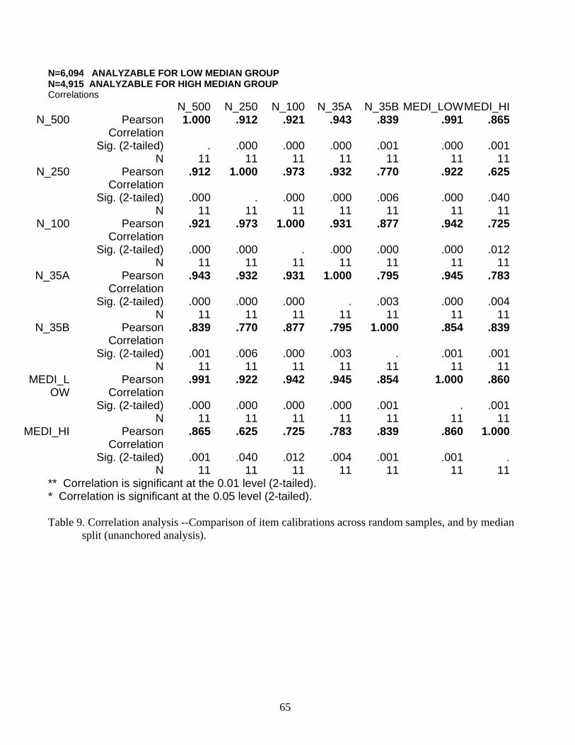
N=6,094 ANALYZABLE FOR LOW MEDIAN GROUP N=4,915 ANALYZABLE FOR HIGH MEDIAN GROUP Correlations
N_500 N_250 N_100 N_35A N_35B MEDI_LOWMEDI_HIN_500 Pearson
Correlation1.000 .912 .921 .943 .839 .991 .865
Sig. (2-tailed) . .000 .000 .000 .001 .000 .001N 11 11 11 11 11 11 11
N_250 PearsonCorrelation
.912 1.000 .973 .932 .770 .922 .625
Sig. (2-tailed) .000 . .000 .000 .006 .000 .040N 11 11 11 11 11 11 11
N_100 PearsonCorrelation
.921 .973 1.000 .931 .877 .942 .725
Sig. (2-tailed) .000 .000 . .000 .000 .000 .012N 11 11 11 11 11 11 11
N_35A PearsonCorrelation
.943 .932 .931 1.000 .795 .945 .783
Sig. (2-tailed) .000 .000 .000 . .003 .000 .004N 11 11 11 11 11 11 11
N_35B PearsonCorrelation
.839 .770 .877 .795 1.000 .854 .839
Sig. (2-tailed) .001 .006 .000 .003 . .001 .001N 11 11 11 11 11 11 11
MEDI_LOW
PearsonCorrelation
.991 .922 .942 .945 .854 1.000 .860
Sig. (2-tailed) .000 .000 .000 .000 .001 . .001N 11 11 11 11 11 11 11
MEDI_HI PearsonCorrelation
.865 .625 .725 .783 .839 .860 1.000
Sig. (2-tailed) .001 .040 .012 .004 .001 .001 .N 11 11 11 11 11 11 11
** Correlation is significant at the 0.01 level (2-tailed). * Correlation is significant at the 0.05 level (2-tailed). Table 9. Correlation analysis --Comparison of item calibrations across random samples, and by median
split (unanchored analysis).
65
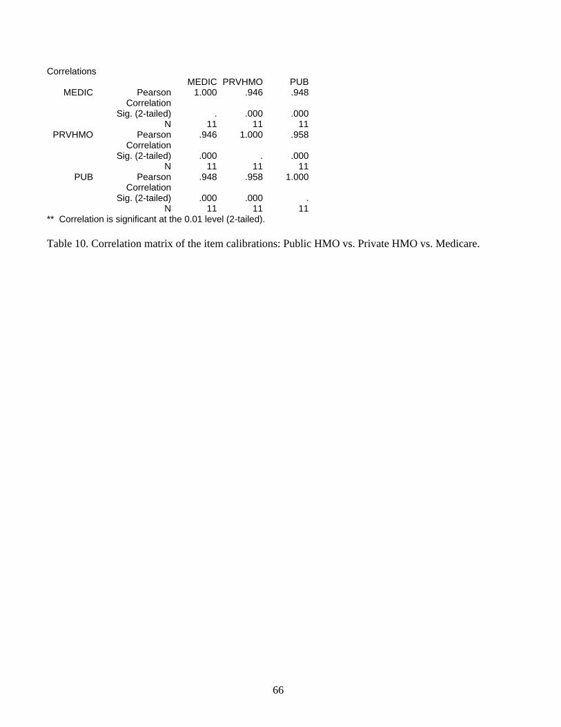
Correlations MEDIC PRVHMO PUB
MEDIC Pearson Correlation
1.000 .946 .948
Sig. (2-tailed) . .000 .000N 11 11 11
PRVHMO Pearson Correlation
.946 1.000 .958
Sig. (2-tailed) .000 . .000N 11 11 11
PUB Pearson Correlation
.948 .958 1.000
Sig. (2-tailed) .000 .000 .N 11 11 11
** Correlation is significant at the 0.01 level (2-tailed). Table 10. Correlation matrix of the item calibrations: Public HMO vs. Private HMO vs. Medicare.
66
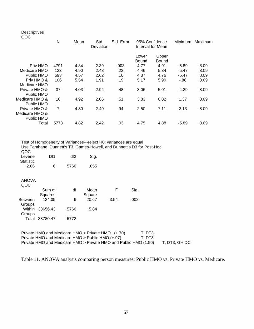
Descriptives QOC
N Mean Std. Deviation
Std. Error 95% Confidence Interval for Mean
Minimum Maximum
Lower Bound
Upper Bound
Priv HMO 4791 4.84 2.39 .003 4.77 4.91 -5.89 8.09 Medicare HMO 123 4.90 2.48 .22 4.46 5.34 -5.47 8.09
Public HMO 693 4.57 2.62 .10 4.37 4.76 -5.47 8.09 Priv HMO &
Medicare HMO106 5.54 1.91 .19 5.17 5.90 -.88 8.09
Private HMO & Public HMO
37 4.03 2.94 .48 3.06 5.01 -4.29 8.09
Medicare HMO & Public HMO
16 4.92 2.06 .51 3.83 6.02 1.37 8.09
Private HMO & Medicare HMO &
Public HMO
7 4.80 2.49 .94 2.50 7.11 2.13 8.09
Total 5773 4.82 2.42 .03 4.75 4.88 -5.89 8.09 Test of Homogeneity of Variances---reject H0: variances are equal Use Tamhane, Dunnett’s T3, Games-Howell, and Dunnett’s D3 for Post-Hoc QOC Levene Statistic
Df1 df2 Sig.
2.06 6 5766 .055 ANOVA QOC
Sum of Squares
df Mean Square
F Sig.
Between Groups
124.05 6 20.67 3.54 .002
Within Groups
33656.43 5766 5.84
Total 33780.47 5772 Private HMO and Medicare HMO > Private HMO (+.70) T, DT3 Private HMO and Medicare HMO > Public HMO (+.97) T, DT3 Private HMO and Medicare HMO > Private HMO and Public HMO (1.50) T, DT3, GH,DC Table 11. ANOVA analysis comparing person measures: Public HMO vs. Private HMO vs. Medicare.
67

MOST MISFITTING RESPONSE STRINGS ITEM OUTMNSQ |PERSON |2222221111 22222111111111111111111 |22222140009777766554403311999888877211110000522222 |66666689921111122416684433700662275644442222353333 |77777454479777600716642288877335465155447777064444 |87654125409210954444367687221521630454984321069875 high-------------------------------------------------- 5 ASKS ABOUT OTH 1.55 A|........................11........................ 2 APPT. WAITING 1.23 B|........................666.......6.6666.......... 11 [NO PROBLEMS] 1.11 C|111111.11..1111...111.....1....................... 9 [EVERYONE HAS 1.03 E|.........11....111......111....1111111111111...... 10 SATIS FAMILY .89 F|..................................3............... 4 LISTENS & GIVES .75 d|......1..............111...1111..............11111 6 CONFIDENT IN PR .44 c|............................................1..... |----------------------------------------------low- Table 12. Using fit statistics to identify inconsistent responses that do not contribute to the measurement
effort.
68
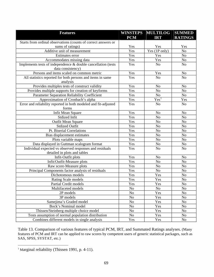
Features WINSTEPS
PCM MULTILOG
IRT SUMMED RATINGS
Starts from ordinal observations (counts of correct answers or sums of ratings)
Yes
Yes
Yes
Additive unit of measurement Yes Yes (1P only) No Estimates error Yes Yes No
Accommodates missing data Yes Yes No Implements tests of independence & double cancellation (tests
data consistency) Yes No No
Persons and items scaled on common metric Yes Yes No All statistics reported for both persons and items in same
analysis Yes No No
Provides multiples tests of construct validity Yes No No Provides multiple supports for creation of keyforms Yes No No
Parameter Separation Reliability Coefficient Yes No No Approximation of Cronbach’s alpha Yes Yes1 Yes
Error and reliability reported in both modeled and fit-adjusted forms
Yes No No
Infit Mean Square Yes No No Stdized Infit Yes No No
Outfit Mean Square Yes No No Stdized Outfit Yes No No
Pt. Biserial Correlations Yes No No Bias displacement estimates Yes No No
Plots variable maps Yes No No Data displayed in Guttman scalogram format Yes No No
Individual expected vs observed responses and residuals detailed in plots and tables
Yes No No
Infit-Outfit plots Yes No No Infit/Outfit-Measure plots Yes No No Raw score-Measure plots Yes No No
Principal Components factor analysis of residuals Yes No No Dichotomous models Yes Yes No Rating Scale models Yes Yes No Partial Credit models Yes Yes No Multifaceted models No No No
2P models No Yes No 3P models No Yes No
Samejima’s Graded model No Yes No Bock’s Nominal model No Yes No
Thissen/Steinberg multiple choice model No Yes No Tests assumption of normal population distribution No Yes No
Combines different models in single analysis Yes Yes No Table 13. Comparison of various features of typical PCM, IRT, and Summated Ratings analyses. (Many features of PCM and IRT can be applied to raw scores by competent users of generic statistical packages, such as SAS, SPSS, SYSTAT, etc.) 1 Marginal reliability (Thissen 1991, p. 4-11).
69
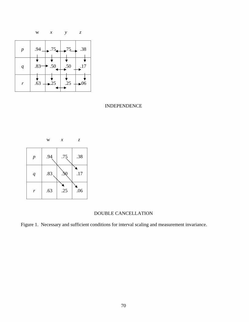
w x y z
p
.94
.75
.75
.38
q
.83
.50
.50
.17
r
.63
.25
.25
.06
INDEPENDENCE
w x z
p
.94
.75
.38
q
.83
.50
.17
r
.63
.25
.06
DOUBLE CANCELLATION
Figure 1. Necessary and sufficient conditions for interval scaling and measurement invariance.
70

MEASURE PERSONS MAP OF QOC ITEMS IN LOGITS
High QOC MARY .############ 6 5 .###### . . . . 4 .######## . . 3 .#
.######## . .#######
. 2 .#######
. .###### 2. Usual wait time for a medical appointment1 (1.59) .#### 3. Phone access (1.29) .### 1. Difficulty in obtaining appointments (1.22) 1 .#### .## 5. Provider asks about treatments other doctors may give2 (0.66) .# .# . 0 .## 10. Satisfied that family members can get needed care (−0.10) TOM . 7. Satisfaction with staff (−0.13) . 11. No difficulty receiving health care (−0.28) . 8. Satisfaction with QOC (−0.43) .# -1 . 9. Everyone in family received care (−0.94) . . 6. Confident in provider ability (−1.38) CINDY . 4. Provider listens and gives information (−1.49) . -2 . . .
Forms of QOC difficult to provide
Noisy items: 1 IMS = 1.3, OMS = 1.2 2 IMS = 1.2, OMS = 1.6
Low QOC
Forms of QOC easy to provide -3 . Figure 2. Variable map. Each ‘#’ is 261 cases; each ‘.’ is less than 261 cases.
71
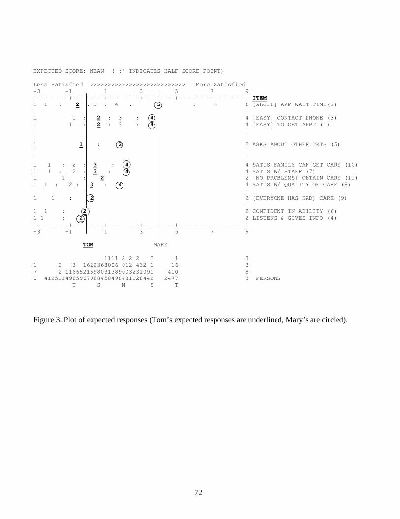
EXPECTED SCORE: MEAN (":" INDICATES HALF-SCORE POINT) Less Satisfied >>>>>>>>>>>>>>>>>>>>>>>>>>> More Satisfied -3 -1 1 3 5 7 9 |---------+---------+---------+---------+---------+---------| ITEM 1 1 : 2 : 3 : 4 : 5 : 6 6 [short] APP WAIT TIME(2) | | 1 1 : 2 : 3 : 4 4 [EASY] CONTACT PHONE (3) 1 1 : 2 : 3 : 4 4 [EASY] TO GET APPT (1) | | | | 1 1 : 2 2 ASKS ABOUT OTHER TRTS (5) | | | | 1 1 : 2 : 3 : 4 4 SATIS FAMILY CAN GET CARE (10) 1 1 : 2 : 3 : 4 4 SATIS W/ STAFF (7) 1 1 : 2 2 [NO PROBLEMS] OBTAIN CARE (11) 1 1 : 2 : 3 : 4 4 SATIS W/ QUALITY OF CARE (8) | | 1 1 : 2 2 [EVERYONE HAS HAD] CARE (9) | | 1 1 : 2 2 CONFIDENT IN ABILITY (6) 1 1 : 2 2 LISTENS & GIVES INFO (4) |---------+---------+---------+---------+---------+---------| -3 -1 1 3 5 7 9 TOM MARY 1111 2 2 2 2 1 3 1 2 3 1622368006 012 432 1 16 3 7 2 1166521598031389003231091 410 8 0 4125114965967068458498481128442 2477 3 PERSONS T S M S T
Figure 3. Plot of expected responses (Tom’s expected responses are underlined, Mary’s are circled).
72

2 Category Items
86420-2-4-6
4 C
ateg
ory
Item
s
10
0
-10
-20 r = .71
Figure 4. QOC person measures, 2 category vs. 4-category items (r=.71, unanchored).
73

-8
-6
-4
-2
0
2
4
6D
iffic
ulty
in o
btai
ning
appo
intm
ents
Usu
al w
ait t
ime
for a
med
ical
app
oint
men
US
C p
hone
acc
ess
US
C li
sten
s an
dgi
ves
info
rmat
ion
US
C a
sks
abou
t tre
atot
her d
ocs
may
giv
e
Con
fiden
t in
US
Cab
ility
Sat
is w
/ US
C s
taff
Sat
is w
ith Q
OC
All
in fa
mily
rec'
dca
re
Sat
isfie
d th
at fa
mily
mem
bers
can
get
ne
No
diffi
culty
rece
ivin
ghe
alth
car
e
QOC ITEM
QO
C IT
EM C
ALI
BR
ATI
ON
n=500 n=250 n=100 n=35A n=35B Low median group High Median Group
Figure 5. Comparison of item calibrations across random samples, and by median split (unanchored
analysis).
74

-5
-4
-3
-2
-1
0
1
2
3
4
5
Diff
icul
ty in
obt
aini
ngap
poin
tmen
ts
Usu
al w
ait t
ime
for a
med
ical
app
oint
men
US
C p
hone
acc
ess
US
C li
sten
s an
dgi
ves
info
rmat
ion
US
C a
sks
abou
t tre
atot
her d
ocs
may
giv
e
Con
fiden
t in
US
Cab
ility
Satis
w/ U
SC s
taff
Sat
is w
ith Q
OC
All
in fa
mily
rec'
d ca
re
Sat
isfie
d th
at fa
mily
mem
bers
can
get
ne
No
diffi
culty
rece
ivin
ghe
alth
car
e
QOC ITEM
QO
C IT
EM C
ALI
BR
ATI
ON
Public HMO Private HMO Medicare
Figure 6. Comparison of QOC item calibrations: Public HMO vs. Private HMO vs. Medicare. N = 562 Public HMO, N = 3539 Private HMO, N = 190 Medicare
75

EXPECTED SCORE OGIVE: MEANS ++-----+-----+-----+-----+-----+-----+-----+-----+-----+-----++ 6 + + | 6666666| 5.5 + 55666 + | 555555 | | E 5 + 5555555 | + X | 55555 * | | P 4.5 + 455 * | + E | 444 | * | | C 4 + 44 | * | + T | 4 * | * | | E 3.5 + 34 * | * | + D | 3| * | * | | 3 + 33 | * | * | + S | 3* | * | * | | C 2.5 + 23 * | * | * | + O | 22 | * | * | * | | R 2 + 22 | * | * | * | + E | 22 * | * | * | * | | 1.5 + 1122 * | * | * | * | + |1111 | * | * | * | * | | 1 + | * | * | * | * | + ++-----+-----+-----+-----+-----+-----+-----+-----+-----+-----++ -4 -3 -2 -1 0 1 2 3 4 5 6 PERSON [MINUS] ITEM MEASURE Figure 7. Plot of non-linear ratings against linear QOC measures, for item 2, Usual wait time for a
medical appointment
76

Person Measure
876543210-1-2-3-4-5-6-7
Per
son
Sco
re3735333129272523211917151311
Figure 8. Plot of scores against linear QOC measures.
77
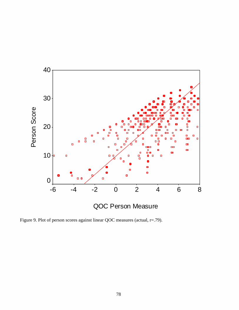
QOC Person Measure
86420-2-4-6
Pers
on S
core
40
30
20
10
0
Figure 9. Plot of person scores against linear QOC measures (actual, r=.79).
78
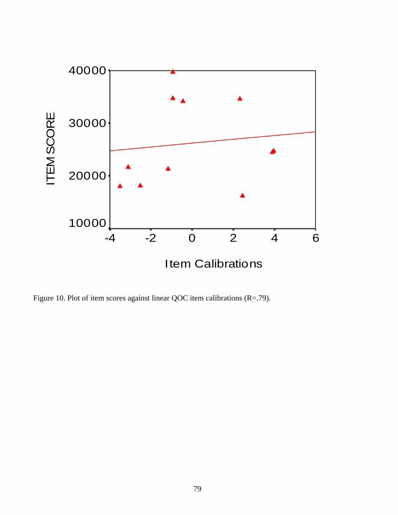
I tem Calibrations
6420-2-4
ITE
M S
CO
RE
40000
30000
20000
10000
Figure 10. Plot of item scores against linear QOC item calibrations (R=.79).
79
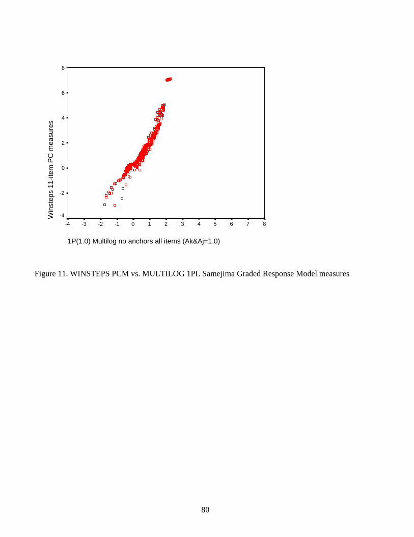
1P(1.0) Multilog no anchors all items (Ak&Aj=1.0)
876543210-1-2-3-4
Win
step
s 11
-item
PC
mea
sure
s
8
6
4
2
0
-2
-4
Figure 11. WINSTEPS PCM vs. MULTILOG 1PL Samejima Graded Response Model measures
80

1P Mlog NoPop MLE measures (Ak&Aj=1.0, items/steps anchored to Winsteps
6543210-1-2-3-4
Win
step
s 11
-item
PC
mea
sure
s6
4
2
0
-2
-4
Figure 12. WINSTEPS PCM vs. MULTILOG 1PL Samejima Graded Response MEPS QOC measures,
with the MULTILOG items anchored at the WINSTEPS values
81

1P(1.8) Multilog no anchors all items (Ak&Aj=1.0)
876543210-1-2-3-4
Win
step
s 11
-item
PC
mea
sure
s
8
6
4
2
0
-2
-4
Figure 13. WINSTEPS PCM vs. MULTILOG 1PL MEPS QOC measures, with the MULTILOG 2d
item parameter fixed at 1.8
82
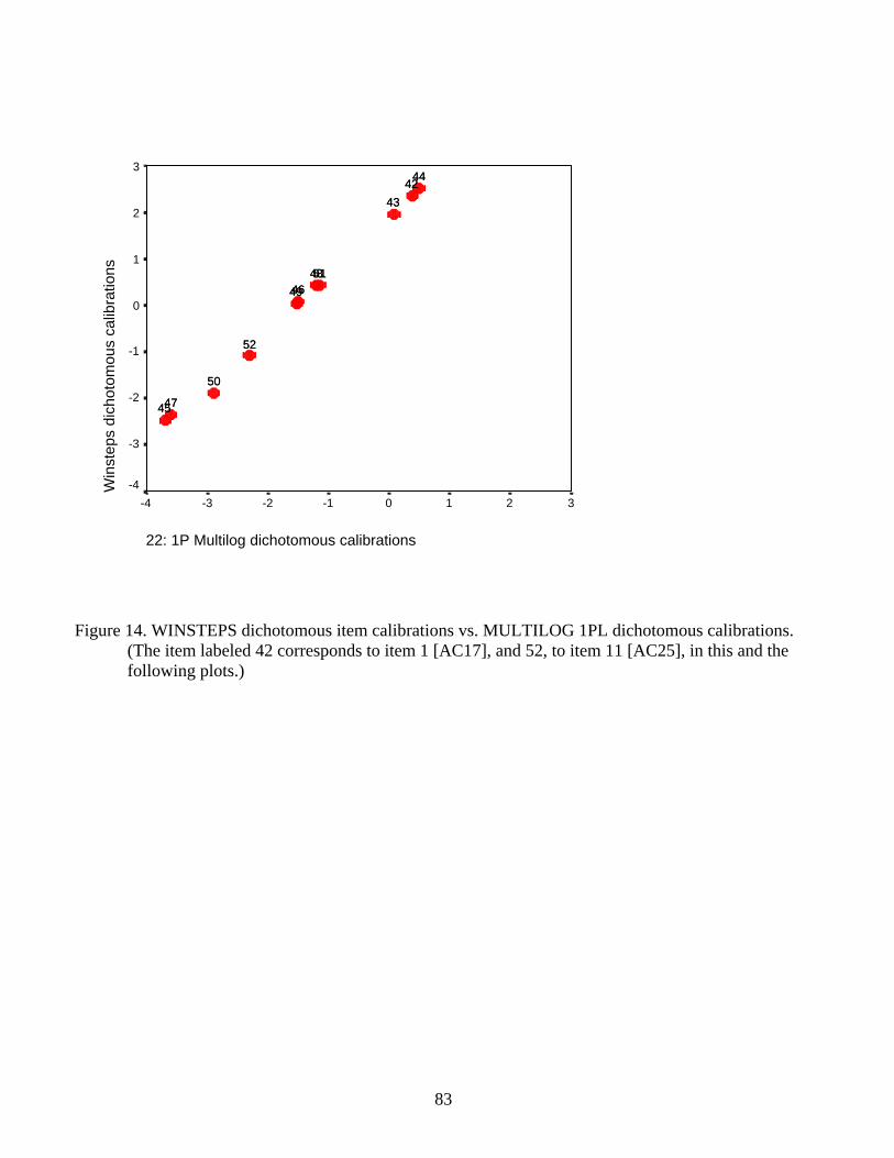
22: 1P Multilog dichotomous calibrations
3210-1-2-3-4
Win
step
s di
chot
omou
s ca
libra
tions
3
2
1
0
-1
-2
-3
-4
444243
48514649
52
50
4745
444243
48514649
52
50
4745
Figure 14. WINSTEPS dichotomous item calibrations vs. MULTILOG 1PL dichotomous calibrations.
(The item labeled 42 corresponds to item 1 [AC17], and 52, to item 11 [AC25], in this and the following plots.)
83

1P Multilog MAP measures all dichot items
6543210-1-2-3-4-5-6
Win
step
s 11
-item
dic
hoto
mou
s m
easu
res
6
4
2
0
-2
-4
-6
Figure 15. WINSTEPS dichotomous MEPS QOC measures vs. MULTILOG 1PL maximum a posteriori
dichotomous measures
84

26: 2P Multilog calibrations (RA PA L2)
3210-1-2-3-4
Win
step
s 11
-item
dic
hoto
mou
s ca
libra
tions
3
2
1
0
-1
-2
-3
-4
444243
485146 49
52
50
4745
444243
485146 49
52
50
4745
Figure 16. WINSTEPS dichotomous MEPS QOC calibrations vs. MULTILOG 2P calibrations (using
marginal maximum likelihood estimation and data input as counts of response patterns).
85
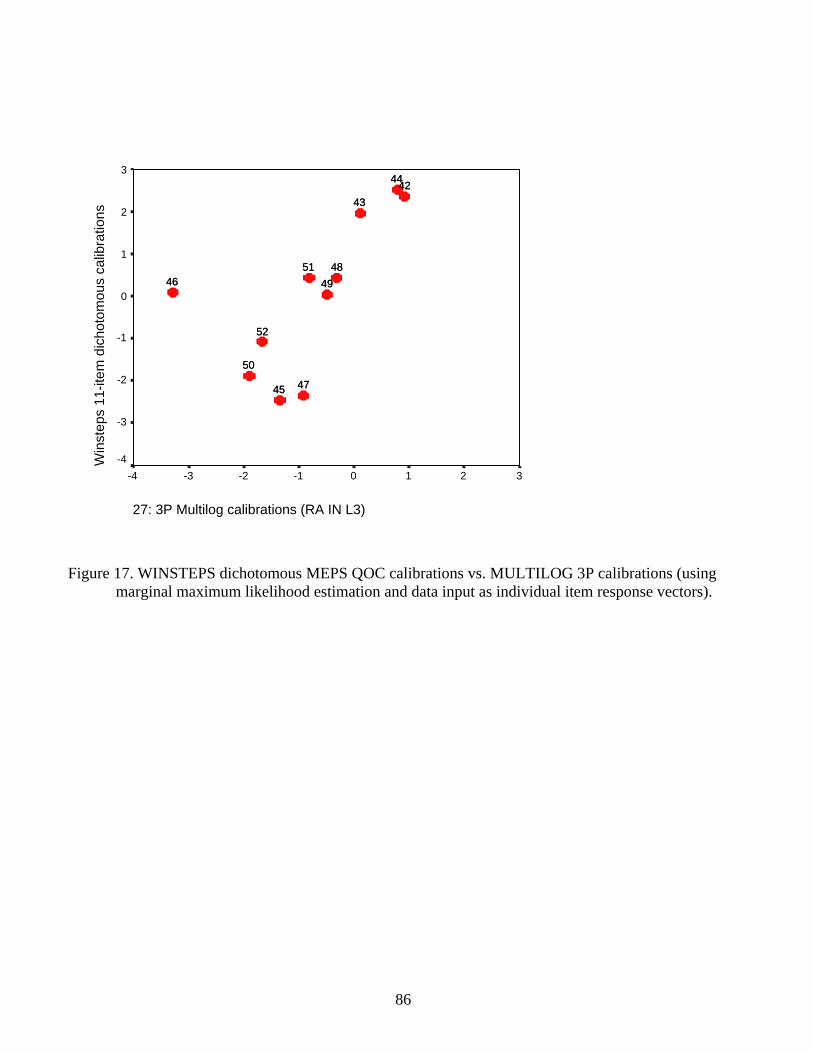
27: 3P Multilog calibrations (RA IN L3)
3210-1-2-3-4
Win
step
s 11
-item
dic
hoto
mou
s ca
libra
tions
3
2
1
0
-1
-2
-3
-4
444243
485146 49
52
50
4745
444243
485146 49
52
50
4745
Figure 17. WINSTEPS dichotomous MEPS QOC calibrations vs. MULTILOG 3P calibrations (using
marginal maximum likelihood estimation and data input as individual item response vectors).
86
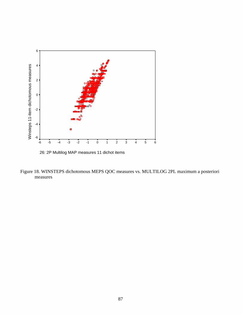
26: 2P Multilog MAP measures 11 dichot items
6543210-1-2-3-4-5-6
Win
step
s 11
-item
dic
hoto
mou
s m
easu
res
6
4
2
0
-2
-4
-6
Figure 18. WINSTEPS dichotomous MEPS QOC measures vs. MULTILOG 2PL maximum a posteriori
measures
87

25: 3P Multilog MAP measures 11 dichot items
6543210-1-2-3-4-5-6
Win
step
s 11
-item
dic
hoto
mou
s m
easu
res
6
4
2
0
-2
-4
-6
Figure 19. WINSTEPS dichotomous MEPS QOC measures vs. MULTILOG 3PL maximum a posteriori
measures
88
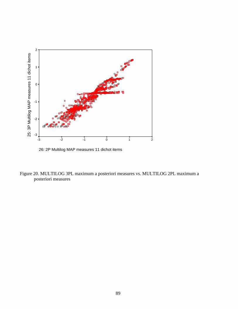
26: 2P Multilog MAP measures 11 dichot items
210-1-2-3
25: 3
P M
ultil
og M
AP
mea
sure
s 11
dic
hot i
tem
s
2
1
0
-1
-2
-3
Figure 20. MULTILOG 3PL maximum a posteriori measures vs. MULTILOG 2PL maximum a
posteriori measures
89

25: 3P Multilog discriminations (RA PA L3)
76543210
27: 3
P M
ultil
og d
iscr
imin
atio
ns (R
A IN
L3)
10
8
6
4
2
0
44
42
43
48
51
46
49
52 50
47
45
44
42
43
48
51
46
49
52 50
47
45
Figure 21. Variation in item discrimination values by type of data input for the MULTILOG 3P model
(PA indicates data input as counts of response patterns; IN indicates data input as individual item response vectors).
90

26: 2P Multilog discriminations (RA PA L2)
543210
25: 3
P M
ultil
og d
iscr
imin
atio
ns (R
A P
A L
3)7
6
5
4
3
2
1
0
44
42
43
4851
46
49
52
50
47
45
44
42
43
4851
46
49
52
50
47
45
Figure 22. Variation in item discrimination parameter estimates in MULTILOG 3P vs. 2P models, using
the same estimation method (marginal maximum likelihood) and the same type of data input (counts of response patterns).
91