Fundamental limits on detection in low SNR

by

Rahul Tandra

B.tech. (Indian Institute of Technology, Bombay) 2003

A thesis submitted in partial satisfactionof the requirements for the degree of

Master of Science

in

Engineering - Electrical Engineering and Computer Sciences

in the

GRADUATE DIVISION

of the

UNIVERSITY OF CALIFORNIA, BERKELEY

Committee in charge:

Professor Anant Sahai, ChairProfessor Micheal Gastpar

Spring 2005

The dissertation of Rahul Tandra is approved.

Chair Date

Date

University of California, Berkeley

Spring 2005

Fundamental limits on detection in low SNR

Copyright c© 2005

by

Rahul Tandra

Abstract

Fundamental limits on detection in low SNR

by

Rahul Tandra

Master of Science in Engineering - Electrical Engineering and Computer Sciences

University of California, Berkeley

Professor Anant Sahai, Chair

In this thesis we consider the generic problem of detecting the presence or absence of a weak

signal in a noisy environment and derive fundamental bounds on the sample complexity of

detection. Our primary motivation for considering the problem of low SNR detection is

the idea of cognitive radios, where the central problem of the secondary user is to detect

whether a frequency band is being used by a known primary user.

By means of examples, we show that the general problem of detecting the presence

or absence of a weak signal is very hard, especially when the signal has no deterministic

component to it. In particular, we show that the sample complexity of the optimal detector

is O(1/SNR2), even when we assume that the noise statistics are completely known.

More importantly we explore the situation when the noise statistics are no longer com-

pletely known to the receiver, i.e., the noise is assumed to be white, but we know its

distribution only to within a particular class of distributions. We then propose a mini-

malist model for the uncertainty in the noise statistics and derive fundamental bounds on

detection performance in low SNR in the presence of noise uncertainty. For clarity of anal-

ysis, we focus on detection of signals that are BPSK-modulated random data without any

pilot tones or training sequences. The results should all generalize to more general signal

constellations as long as no deterministic component is present.

1

Specifically, we show that for every ‘moment detector’ there exists an SNR below which

detection becomes impossible in the presence of noise uncertainty. In the neighborhood of

that SNR wall, we show how the sample complexity of detection approaches infinity. We

also show that if our radio has a finite dynamic range (upper and lower limits to the voltages

we can quantize), then at low enough SNR, any detector can be rendered useless even under

moderate noise uncertainty.

Professor Anant SahaiDissertation Committee Chair

2

Dedicated to my parents.

i

Contents

Contents ii

List of Figures iv

List of Tables vi

Acknowledgements vii

1 Introduction 1

2 Detection in Gaussian noise 7

2.1 Introduction . . . . . . . . . . . . . . . . . . . . . . . . . . . . . . . . . . . . 7

2.2 Problem formulation . . . . . . . . . . . . . . . . . . . . . . . . . . . . . . . 8

2.3 Sample complexity of signal detection under WGN . . . . . . . . . . . . . . 9

2.3.1 Matched filter . . . . . . . . . . . . . . . . . . . . . . . . . . . . . . . 9

2.3.2 Radiometer . . . . . . . . . . . . . . . . . . . . . . . . . . . . . . . . 10

2.3.3 Sinusoidal signals . . . . . . . . . . . . . . . . . . . . . . . . . . . . . 10

2.3.4 BPSK detection . . . . . . . . . . . . . . . . . . . . . . . . . . . . . 15

2.4 Pilot signals . . . . . . . . . . . . . . . . . . . . . . . . . . . . . . . . . . . . 18

2.4.1 BPSK signal with a weak pilot . . . . . . . . . . . . . . . . . . . . . 18

3 Noise Uncertainty 21

3.1 Introduction . . . . . . . . . . . . . . . . . . . . . . . . . . . . . . . . . . . . 21

3.2 Need for an uncertainty model . . . . . . . . . . . . . . . . . . . . . . . . . 22

3.3 Noise uncertainty model . . . . . . . . . . . . . . . . . . . . . . . . . . . . . 23

3.3.1 The problem of detection under uncertainty . . . . . . . . . . . . . . 24

3.4 Implications of noise uncertainty . . . . . . . . . . . . . . . . . . . . . . . . 25

ii

3.5 Discussion of results . . . . . . . . . . . . . . . . . . . . . . . . . . . . . . . 29

3.6 Approaching the SNR wall . . . . . . . . . . . . . . . . . . . . . . . . . . . . 33

3.7 Other possible noise uncertainty models . . . . . . . . . . . . . . . . . . . . 33

3.7.1 Discussion . . . . . . . . . . . . . . . . . . . . . . . . . . . . . . . . . 39

4 Finite Dynamic Range and Quantization 42

4.1 Introduction . . . . . . . . . . . . . . . . . . . . . . . . . . . . . . . . . . . . 42

4.2 Motivating example: 2-bit quantizer . . . . . . . . . . . . . . . . . . . . . . 43

4.3 Finite dynamic range: absolute walls . . . . . . . . . . . . . . . . . . . . . . 45

4.4 Discussion . . . . . . . . . . . . . . . . . . . . . . . . . . . . . . . . . . . . . 49

5 Comments and Conclusions 52

Bibliography 55

References . . . . . . . . . . . . . . . . . . . . . . . . . . . . . . . . . . . . . . . . 55

A Appendix: Sample complexity of BPSK detector 57

A.0.1 Detection Performance using the Central Limit Theorem . . . . . . 57

iii

List of Figures

1.1 Instance of the hidden terminal problem. The blue antennas correspond to the primary

system and the red antenna corresponds to the cognitive radio that is shadowed with respect

to the primary transmitter. . . . . . . . . . . . . . . . . . . . . . . . . . . . . . . 3

1.2 Abstraction of the detection problem . . . . . . . . . . . . . . . . . . . . . . . . . 4

2.1 The sample complexities of the various detectors discussed in section 2.3 are plotted in this

figure. These curves (read from top to bottom in the figure) were obtained by using the

sample complexities derived in the equations (2.5), (2.12), (2.11), (2.7) and (2.4) respectively. 16

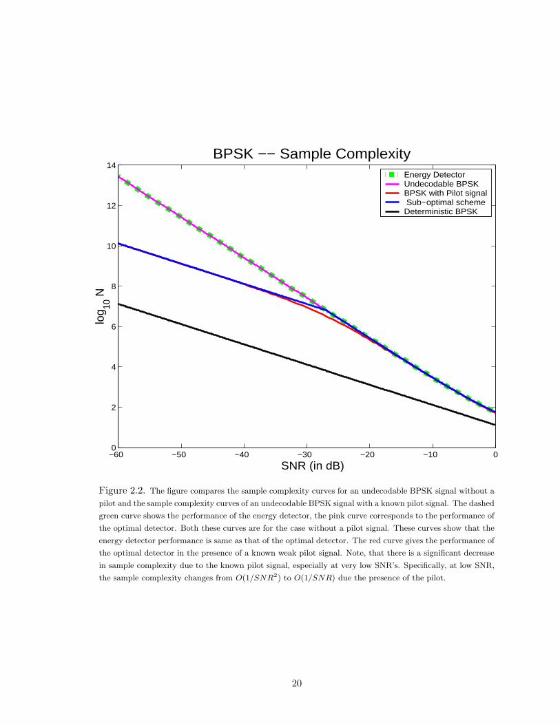
2.2 The figure compares the sample complexity curves for an undecodable BPSK signal without

a pilot and the sample complexity curves of an undecodable BPSK signal with a known

pilot signal. The dashed green curve shows the performance of the energy detector, the pink

curve corresponds to the performance of the optimal detector. Both these curves are for

the case without a pilot signal. These curves show that the energy detector performance is

same as that of the optimal detector. The red curve gives the performance of the optimal

detector in the presence of a known weak pilot signal. Note, that there is a significant

decrease in sample complexity due to the known pilot signal, especially at very low SNR’s.

Specifically, at low SNR, the sample complexity changes from O(1/SNR2) to O(1/SNR)

due the presence of the pilot. . . . . . . . . . . . . . . . . . . . . . . . . . . . . . 20

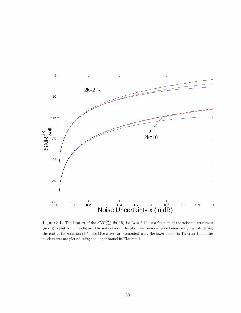
3.1 The location of the SNR(2k)wall

(in dB) for 2k = 2, 10, as a function of the noise uncertainty x

(in dB) is plotted in this figure. The red curves in the plot have been computed numerically

by calculating the root of the equation (3.7), the blue curves are computed using the lower

bound in Theorem 1, and the black curves are plotted using the upper bound in Theorem 1. 30

3.2 This figure pictorially depicts the two hypothesis and the threshold in a 2k-th moment

detector. The figure on the top shows the case when there is no noise uncertainty and the

one in the bottom is the case when there is noise uncertainty. Note that under noise uncer-

tainty and sufficiently weak signal power, there is an overlap region under both hypotheses,

which renders the detector useless. . . . . . . . . . . . . . . . . . . . . . . . . . . 32

3.3 This figure shows the sample complexity of the moment detectors (number of samples as a

function of SNR) at a moderate noise uncertainty of x = 0.5 dB. The curves in this figure

have been computed using the equation (3.11) . . . . . . . . . . . . . . . . . . . . . 34

iv

3.4 Variation of snr∗wall is plotted as a function of the noise uncertainty x. The green curve is

a plot of the snr∗wall. This curve has been obtained by numerically finding the minimum

of snr(2k0)wall

for a large range of values of k0. The red curve in the plot is the upper bound

for snr∗wall obtained in (3.21). These curves are compared with the blue curve which is

the snrwall for the radiometer under the minimalist uncertainty model in theorem 1. Note

that all the curves lie on top of each other. This shows that (3.23) is indeed true. . . . . 40

3.5 The red curves are plots of snr(2k)wall

as a function of k for three different values of x. These

plots show that, snr(2k)wall

is monotonically increasing for k > 0 and hence its minimum is

attained at k = 1. The green curves are an upper bound for snr(2k)wall

given by α2k−1

k. . . 41

4.1 2-bit quantizer . . . . . . . . . . . . . . . . . . . . . . . . . . . . . . . . . . . . 44

4.2 The plot on the top shows the variation of the SNRwall with noise uncertainty x and the

plot on the bottom is the sample complexity of the optimal detector for a 2-bit quantizer,

with three different values of the noise uncertainty x. Note, that even at a very low noise

uncertainty of x = 0.1 dB, the SNRwall is at a relatively high value of −17 dB. . . . . . 46

4.3 The density functions of the constructed noise random variable in both cases to prove

theorem 3 is shown in this figure. The figure on the left corresponds to Case I discussed

in section 4.3. Note that there are two delta functions in the density of Wa at ±M . The

figure on the right corresponds to case II in section 4.3. In this figure note that there is

a small hole in the density function of Wa at ±M . In both these figures, the red curve

corresponds to the density function of Wa and the black curve corresponds to the density

function of Wn. . . . . . . . . . . . . . . . . . . . . . . . . . . . . . . . . . . . 50

v

List of Tables

4.1 We list kmin as a function of the finite dynamic range M for two different values of the

noise uncertainty x. For each value of M , kmin has been numerically computed such

thatEW

2ka I|Wa|<M +M

2kP(|Wa|=M)

EW2kn

< (α − 1). Also, the SNRwall has been computed from

equation (4.9) for each value of kmin. . . . . . . . . . . . . . . . . . . . . . . . . 49

vi

Acknowledgements

I would like to thank my advisor, Prof. Anant Sahai for his encouragement and inspirational

guidance. The time spent in the several meetings with my advisor has been a great learning

experience for me. I would also like to thank Prof. Micheal Gastpar, Prof. David Tse, Prof.

Kannan Ramchandran and the students in the spectrum sharing group, from whom I have

learned a lot during the 3R meetings.

vii

Chapter 1

Introduction

The subject of signal detection and estimation deals with the processing of information-

bearing signals in order to make inferences about the information that they contain. This

field traces its origin from the classical work of Bayes [1], Gauss [10], Fisher [7], and Neyman

and Pearson [21], on statistical inference. However, the theory of detection took hold as a

recognizable discipline only from the early 1940’s. Presumably, signal detection has a wide

range of applications including communications. The work of Price and Abramson [22], is

one of the early efforts highlighting the importance of signal detection in communications

and a comprehensive survey of the results and techniques of detection theory developed in

the past decades can be found in [15].

In this thesis we are interested in the problem of detecting the presence or absence

of a signal in a noisy environment. Throughout this thesis, whenever we refer to ‘signal

detection’, we mean detecting the presence of a signal in background noise. We mainly

concentrate on two types of signal detection problems, i) detecting known signals in additive

noise (coherent detection), and ii) random signals in additive noise (non-coherent detection).

For example, receivers which try to pickup a known pilot signal/training data sent by a

transmitter use coherent detection. In this case, the receiver knows the exact signal and

hence the optimal detector is just a matched filter [19]. On the other hand, one of the most

common example of a non-coherent detector is an energy detector (radiometer). It is known

1

that the radiometer is the optimal detector when the receiver knows only the power of the

signal [25], [29].

As the title of the thesis suggests, we are mainly interested in the problem of detecting

very low SNR signals in additive noise. Our interest in the very low SNR regime is motivated

by the possibility for cognitive radios [6], [20]. Cognitive radio refers to wireless architectures

in which a communication system does not operate in a fixed assigned band, but rather

searches and finds an appropriate band in which to operate. This represents a new paradigm

for spectrum utilization in which new devices can opportunistically scavenge bands that are

not being used at their current time and location for their primary purpose [5]. This is

inspired by actual measurements showing that most of the allocated spectrum is vastly

underutilized [2].

One of the most important requirement for any cognitive radio system is to provide a

guarantee that it would not interfere with the primary transmission. In order to provide

such a guarantee it is obvious that a cognitive radio system should be able to detect the

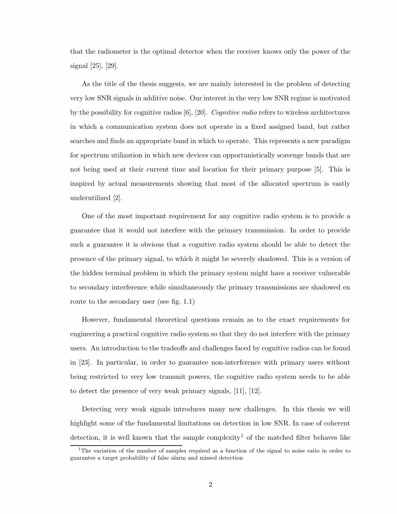
presence of the primary signal, to which it might be severely shadowed. This is a version of

the hidden terminal problem in which the primary system might have a receiver vulnerable

to secondary interference while simultaneously the primary transmissions are shadowed en

route to the secondary user (see fig. 1.1)

However, fundamental theoretical questions remain as to the exact requirements for

engineering a practical cognitive radio system so that they do not interfere with the primary

users. An introduction to the tradeoffs and challenges faced by cognitive radios can be found

in [23]. In particular, in order to guarantee non-interference with primary users without

being restricted to very low transmit powers, the cognitive radio system needs to be able

to detect the presence of very weak primary signals, [11], [12].

Detecting very weak signals introduces many new challenges. In this thesis we will

highlight some of the fundamental limitations on detection in low SNR. In case of coherent

detection, it is well known that the sample complexity1 of the matched filter behaves like

1The variation of the number of samples required as a function of the signal to noise ratio in order toguarantee a target probability of false alarm and missed detection

2

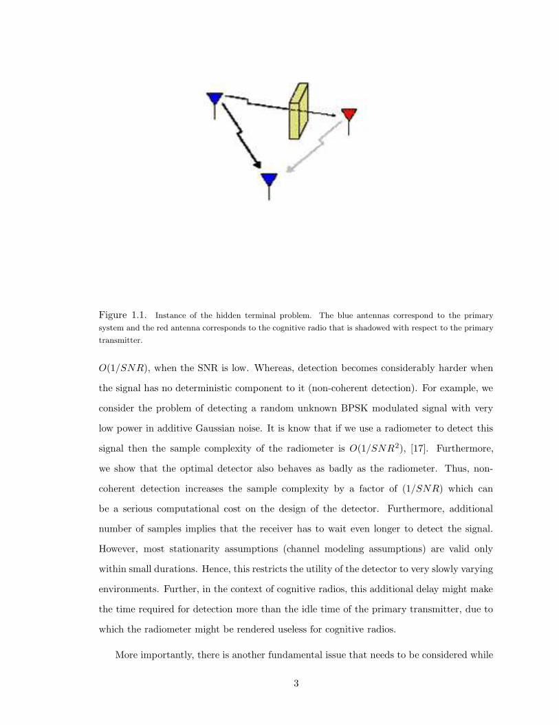
Figure 1.1. Instance of the hidden terminal problem. The blue antennas correspond to the primary

system and the red antenna corresponds to the cognitive radio that is shadowed with respect to the primary

transmitter.

O(1/SNR), when the SNR is low. Whereas, detection becomes considerably harder when

the signal has no deterministic component to it (non-coherent detection). For example, we

consider the problem of detecting a random unknown BPSK modulated signal with very

low power in additive Gaussian noise. It is know that if we use a radiometer to detect this

signal then the sample complexity of the radiometer is O(1/SNR2), [17]. Furthermore,

we show that the optimal detector also behaves as badly as the radiometer. Thus, non-

coherent detection increases the sample complexity by a factor of (1/SNR) which can

be a serious computational cost on the design of the detector. Furthermore, additional

number of samples implies that the receiver has to wait even longer to detect the signal.

However, most stationarity assumptions (channel modeling assumptions) are valid only

within small durations. Hence, this restricts the utility of the detector to very slowly varying

environments. Further, in the context of cognitive radios, this additional delay might make

the time required for detection more than the idle time of the primary transmitter, due to

which the radiometer might be rendered useless for cognitive radios.

More importantly, there is another fundamental issue that needs to be considered while

3

Frequency

converterdown−

Low−noiseamplifier

Intermediatefrequencyamplifier

A/DConverter Detector

Receivingantenna

Figure 1.2. Abstraction of the detection problem

detecting signals in low SNR’s. The classical Bayes, minimax and Neyman-Pearson design

strategies for optimum signal detection and other decision strategies require a complete

statistical description of the data in order to specify the optimum decision rule structure.

However, there is frequently some uncertainty concerning the statistical structure of the

data, for example the additive Gaussian noise assumption in our problem is only an approxi-

mation. It has been demonstrated that procedures designed around a particular model may

perform poorly when actual data statistics differ from those assumed. For example, the per-

formance of optimum procedures designed under the assumption of Gaussian distributions

are often considerably degraded for slight deviations from the Gaussian assumption [28].

Furthermore, we claim that the degradation in performance is worsened in the low SNR

regime.

To deal with situations mentioned above it is often of interest to find decision procedures

which are robust, that is, which perform well despite small variations from the assumed sta-

tistical model. There were several studies which considered the design of robust detectors.

The statistical work of Huber in estimation [13] and hypothesis testing [14] are generally

regarded as the starting point of the area of minimax robustness. Huber considered the

problem of robustly testing a simple hypothesis H0 against a simple alternative H1, assum-

ing that the true underlying densities q0 and q1 lie in some neighborhood of the idealized

model densities p0 and p1, respectively, and that they are related by

qi = (1 − εi)pi(x) + εihi(x), i = 0, 1 hi ∈ H (1.1)

where 0 ≤ εi < 1 are fixed numbers and H denotes the class of all density functions.

4

As Huber showed, this problem has a solution (existence of a robust detection procedure),

when the εi are small enough, so that it is impossible for the distribution classes defined

by (1.1) to overlap.

This work has been successfully applied to a long sequel of problems in detection and

estimation, e.g., the works of Martin and Schwartz [18], Kassam and Thomas [16], and

El-Sawy and Vandelinde [4]. Specifically, Martin and Schwartz consider the problem of

detecting a signal of known form in additive, nearly Gaussian noise, and they derive a robust

detector when the signal amplitude is known and the nearly Gaussian noise is specified by

Huber’s mixture model.

It is important to note that as the previous works mentioned above have considered the

problem of detecting the presence or absence of known signals under noise uncertainty, i.e.,

they try to derive a robust coherent detector. However, the model considered by Huber is

more general and can be applied to non-coherent detection also. In this thesis, we propose

a similar model for the noise uncertainty, which can be shown to be a special case of the

model given in (1.1). However, since we are interested in detection in low SNR, it is not

reasonable to assume that the distribution classes under both the hypotheses don’t overlap.

In fact, we show that under sufficiently low SNR, the distribution classes must overlap,

which in turn leads to serious limitations on the prospect of robust detection. Sonnenschein

and Fishman [26], analyze the affect of noise power uncertainty in radiometric detection of

spread-spectrum signals and identify a fundamental limit on the SNR of the signals we can

detect. We extend their results beyond the energy detector to detectors that examine other

moments.

Furthermore, we show that the fundamental limits on moment detectors become hard

limits on any possible detector if the radio has a finite dynamic range on its input. This

result says that under the finite dynamic range assumption it is impossible to find any

robust detector below a certain SNR threshold. Intuitively, this result arises because, under

the finite dynamic range assumption and in low SNR, the distribution classes under both

hypothesis must overlap for any possible detector, i.e., it is possible for a noise distribution

in each hypothesis to mimic the nominal distribution in the other hypothesis, thus leading

5

to impossibility in signal detection. Since all physical radios have such a limit, we feel that

the bounds here represent important constraints on practical systems.

In the next chapter, we formulate the detection problem as a hypothesis testing problem

and discuss the sample complexity of various detectors, under the additive Gaussian noise

assumption. In this chapter we assume that the noise statistics are completely known to the

receiver. Chapter 3 relaxes this constraint and we build a model for the noise uncertainty.

Under our model we show that for every moment detector there exists a SNR below which

detection becomes impossible. We extend this impossibility result for a generic detector

in chapter 4, where we make the practical assumption that our receivers are limited to a

finite dynamic range of operation. Finally, we conclude by giving a brief discussion of the

signal detection problem when the signal is no longer white. We give some arguments which

suggest that even robust detectors (like feature detectors) might have to face the practical

limitations of noise uncertainty. However, we feel that the limits in this case arise due to

the uncertainty in the whiteness assumption of noise (in practice noise is also never white!).

Therefore, we feel that these limitations are very fundamental in nature and systems which

work under the very low SNR regime (like cognitive radios) cannot escape such limitations.

6

Chapter 2

Detection in Gaussian noise

2.1 Introduction

We start off by formulating the general problem of detecting the presence or absence

of a signal in additive noise as a binary hypothesis testing problem. In the most general

formulation we allow for the noise process to lie in a class of distributions around the nominal

distribution.

However, as a preliminary discussion to the general problem we first assume that the

noise statistics is completely known to the receiver. We assume that the noise is white

Gaussian, and is independent of the signal. Under these assumptions we derive the sample

complexities of optimal detectors1 for various classes of signals and compare them with the

sample complexity of the corresponding matched filter and radiometer.

Before we begin our discussion of signal detection, we first point out the critical dif-

ferences between detection and demodulation. By demodulation, we mean the process of

decoding a message based on the received signal. Shannon in his landmark paper [24],

showed that it is possible to reliably demodulate the signal only if the rate of transmission

is below a certain threshold, what we now call the Shannon capacity of the channel. The

1Note that the notion of optimality is in the classical Neyman-Pearson sense, i.e., a detector is optimal ifit minimizes the number of samples required for detection subject to given target probabilities of false alarmand missed detection constraints

7

main problem in demodulation is to decode the transmitted message from the received (pos-

sibly corrupted) signal. However, we are already assuming the presence of a transmission

in demodulation, i.e., the receiver knows that there is a primary signal present and all it

has to do is to figure out what it is.

On the other hand, detecting signals at very low SNR is the main focus of this thesis.

In particular we assume that the SNR is so low that we are operating below the capacity of

the channel. Thus demodulating the signal is not possible, and we can only hope to detect

the signal. In our problem the important case is detecting the absence of the primary signal.

This is a hard problem, since there is no easy way to prove the absence of a signal. The

only possible way to do this is to contradict the fact that there is a primary transmission

present. However, contradicting the presence of a signal is hard when the signal power is

very low. Therefore, the problem of detection is considerably harder than demodulation.

2.2 Problem formulation

The problem of signal detection in additive noise can be formulated as a binary hypoth-

esis testing problem with the following hypotheses:

H0 : Y [n] = W [n] n = 1, . . . , N

H1 : Y [n] = X[n] + W [n] n = 1, . . . , N (2.1)

where X[n] and W [n] are the signal and noise samples respectively. We assume that both

the signal and noise processes are white and are independent of each other. However,

we allow for the noise process to have any distribution from a class of noise distributions

W. Without loss of generality we can assume that W is centered around a nominal noise

distribution Wn.

Given a particular target probability of false alarm PFA and probability of missed de-

tection PMD, our aim is to derive the sample complexities for various possible detectors,

i.e., we are interested in calculating the number of samples required N , as a function of the

8

signal to noise ratio, which is defined as

snr =EX2

1

EW 2n

SNR = 10 log10

(EX2

1

EW 2n

)(2.2)

For notational convenience, an upper case SNR is used to denote the signal to noise ratio

in decibels. Also, since the noise distribution can lie within the class W, we define snr with

respect to the nominal noise distribution Wn as given in (2.2). In particular we are interested

in the sample complexity of the optimal detector, i.e., the detector which minimizes N , for

a given PFA and PMD.

2.3 Sample complexity of signal detection under WGN

Now, we consider the following hypothesis testing problem:

H0 : Y [n] = W [n] n = 0, 1, . . . , N − 1

H1 : Y [n] = X[n] + W [n] n = 0, 1, . . . , N − 1 (2.3)

Here we assume that W [n]’s are samples from a white Gaussian noise process with power

spectral density σ2, i.e., W [n] ∼ N(0, σ2). This is a special case of the general problem

in (2.1) with no uncertainty in the noise process and its statistics are completely know to

the receiver.

We restrict ourselves to this model throughout this section. We start with the most

simplest version of the problem: the case when the signal X[n] is completely known to the

receiver. Then, we make the problem progressively harder by dropping some of the simpli-

fying assumptions made above and derive the sample complexity of the optimal detector in

each case.

2.3.1 Matched filter

Here we assume that the signal samples X[n] in (2.3) are completely known to the

receiver. In this case, the optimal detector is

T (Y) =N−1∑

n=0

Y [n]X[n]H1

≷H0

γ

9

This detector is referred to as a correlator or the matched filter. It can easily be shown

that [17],

N = [Q−1(PD) − Q−1(PFA)]2(snr)−1

= O(snr−1) (2.4)

Thus we see that the number of samples required varies as O(1/snr).

2.3.2 Radiometer

Now, we consider a completely opposite problem to the one in section 2.3.1. Here we

assume absolutely no deterministic knowledge about the signal X[n], i.e., we assume that

we know only the average power in the signal.

In this case the optimal detector is

T (Y) =

N−1∑

n=0

Y 2[n]H1

≷H0

γ

that is, we computes the energy in the signal and compare it to a threshold. Hence it is

known as an energy detector or radiometer. In this case, it is easy to verify that [17],

N = 2[(Q−1(PFA) − Q−1(PD))snr−1 − Q−1(PD)

]2

= O(snr−2) (2.5)

Thus the number of samples, N varies as O(1/snr2) for the energy detector.

2.3.3 Sinusoidal signals

Now we assume that the signal X[n] = A cos(2πf0n + φ) in (2.3), i.e., we consider the

following detection problem:

H0 : Y [n] = W [n] n = 0, 1, . . . , N − 1

H1 : Y [n] = A cos(2πf0n + φ) + W [n] n = 0, 1, . . . , N − 1 (2.6)

Here we consider the cases when any subset of the parameter set {A, f0, φ} may be un-

known. We assume that these parameters are fixed but unknown in (2.6) and hence use the

Generalized Likelihood Ratio Test (GLRT) (see [17]) for the following cases.

10

1. A unknown

2. A, φ unknown

3. A, φ, f0 unknown

We solve each of the following cases in order.

Amplitude unknown

Here we assume that A is unknown (2.6). The GLRT decides H1 if,

f(Y, A|H1)

f(Y|H0)> γ

where A is the Maximum Likelihood Estimate (MLE) of A under H1, i.e.,

A = arg maxA

f(Y, A|H1)

= arg maxA

1

(2πσ2)N

2

exp

[− 1

2σ2

N−1∑

n=0

(Y [n] − AX[n])2

]

= arg minA

N−1∑

n=0

(Y [n] − AX[n])2

=

∑N−1n=0 Y [n]X[n]∑N−1

n=0 X2[n]

Using this A to calculate the likelihood ratio we have the following detection rule

T (Y) =

(N−1∑

n=0

Y [n]X[n]

)2H1

≷H0

γ

The performance of this detector can be easily calculated and we get

PD = Q(Q−1

(PFA

2

)−

√N · snr) + Q(Q−1

(PFA

2

)+

√N · snr) (2.7)

It can be observed from the above equation that for a fixed PFA and PD, the number

of samples N varies as snr−1. Thus even when the amplitude is unknown the sample

complexity varies as O(1/snr).

11

Unknown Amplitude and phase

Now, we assume that both A and φ are unknown in (2.6). As before we use the GLRT

and decide upon H1 if

LG(Y) =f(Y, A, φ|H1)

f(Y|H0)> γ (2.8)

where A, φ are the MLE’s of A and φ under H1 respectively, i.e.,

(A, φ) = arg max(A,φ)

f(Y, A, φ|H1)

= arg max(A,φ)

1

(2πσ2)N

2

exp

[− 1

2σ2

N−1∑

n=0

(Y [n] − A cos(2πf0n + φ))2

]

= arg min(A,φ)

N−1∑

n=0

(Y [n] − A cos(2πf0n + φ))2

= arg min(α1 ,α2)

N−1∑

n=0

(Y [n] − α1 cos(2πf0n) − α2 sin(2πf0n))2

Where α1 = A cos(φ) and α2 = −A sin(φ). We can easily optimize the above expression

and obtain the MLE’s of A and φ to be

A =√

α1 + α2

φ = arctan(− α2

α1)

where,

α1 ≈ 2

N

N−1∑

n=0

Y [n] cos(2πf0n)

α2 ≈ 2

N

N−1∑

n=0

Y [n] sin(2πf0n)

for f0 not near 0 or 12 . Note that we can choose any f0 ∈ (0, 1

2) by sampling the original

continuous time sinusoid at a suitable frequency greater than the Nyquist frequency.

Substituting the MLE’s in (2.8) and taking logarithm we get

lnLG(Y) = − 1

2σ2

[N−1∑

n=0

−2Y [n]A cos(2πf0n + φ) +N−1∑

n=0

A2 cos2(2πf0n + φ)

]

12

Using the parameter transformation we have α1 = A cos(φ), α2 = A sin(φ) so that

N−1∑

n=0

Y [n]A cos(2πf0n + φ)

=N−1∑

n=0

Y [n] cos(2πf0n)A cos α1 −N−1∑

n=0

Y [n] sin(2πf0n)A sin α1

=N

2(α1

2 + α22)

Also, making use ofN−1∑

n=0

cos2(2πf0n + φ) ≈ N

2

results in

lnLG(x) = − 1

2σ2

[−2

N

2(α1

2 + α22) +

N

2A2

]

= − 1

2σ2

[−N

2(α1

2 + α22)

]

=N

4σ2(α1

2 + α22) (2.9)

or we decide H1 if

N

4σ2(α1

2 + α22) > ln γ

⇒ N

4σ2

(2

N

)2(

N−1∑

n=0

Y [n] cos(2πf0n)

)2

+

(N−1∑

n=0

Y [n] sin(2πf0n)

)2 > ln γ

⇒ 1

σ2

1

N

∣∣∣∣∣

N−1∑

n=0

Y [n] exp (−j2πf0n)

∣∣∣∣∣

2

> lnγ

⇒ 1

σ2I(f0) > ln γ (2.10)

where I(f0) is the periodogram evaluated at f = f0. Thus, the sample complexity in this

case turns out to be

PD = QX ′22(λ)

(2 ln

1

PFA

)(2.11)

where λ = N · snr and QX ′22(λ) is the tail probability of the standard chi-squared random

variable with 2 degrees of freedom and noncentrality parameter λ. It is clear that N · snr

is the only variable in the above equation for fixed PFA and PD. Thus, in this case also the

sample complexity varies as O(1/snr)

13

Amplitude, phase and frequency unknown

Now, we assume that the frequency f0 is also unknown in (2.6). Here we assume that

the continuous time frequency of the signal f can lie anywhere from (0, fmax). However, by

sampling at a greater rate than 2fmax we can also make sure that the discrete frequency

f0 lies in (0, 12). Therefore there is only a bounded set of uncertainty in the frequency

of the discrete time signal. Similarly assuming that the original continuous time signal is

within a narrow band (f −W,f +W ) does not help too much, because the frequency of the

discrete time signal will again lie in (0, 12). To summarize, the amount of uncertainty in the

frequency is not a real issue while detection discrete time signals. Now, we try to solve the

detection problem assuming that f0 ∈ (0, 12).

When the frequency is also unknown in (2.6), the GLRT decides H1 if

f(Y, A, φ, f0|H1)

f(x|H0)> γ

or

maxf0 f(Y, A, φ, f0|H1)

f(x|H0)> γ

Since the PDF under H0 does not depend on f0 and is nonnegative, we have

maxf0

f(Y, A, φ, f0|H1)

f(x|H0)> γ

taking the logarithm in the above inequality, we have

lnmaxf0

f(Y, A, φ, f0|H1)

f(x|H0)> ln γ

and by monotonicity of log we can write this as

maxf0

lnf(Y, A, φ, f0|H1)

f(x|H0)> ln γ

but from (2.10) we have

lnf(Y, A, φ, f0|H1)

f(x|H0)=

I(f0)

σ2

so finally we decide H1 if

maxf0

I(f0) > σ2 ln γ = γ′

14

Thus, this detector detects that the signal is present if the peak of the periodogram exceeds

a threshold. Assuming that an N -point FFT is used to evaluate I(f) and that the maximum

is found over the frequencies fk = kN for k = 1, 2, . . . , N

2 − 1, we have that

PD = QX ′22(λ)

(2 ln

N2 − 1

PFA

)(2.12)

Here we assume that the actual frequency f0 is a multiple of 1N . Clearly there will be some

loss if f0 is not near a multiple of 1N .

Fig. 2.1 plots the sample complexities of all the examples discussed in this section.

Observe that the radiometer and the matched filter have the best and the worst sample

complexities respectively, while the rest of the cases lie strictly between them. Also, observe

that the lack of knowledge of frequency of a sinusoid does not affect the sample complexity

by much. The sample complexity is still quite close to O(1/snr) as seen in the figure.

2.3.4 BPSK detection

We have shown that the radiometer is the worst case possible. This is expected because

the radiometer assumes minimal knowledge about the signal, namely only the average power

in the signal. The cost paid is an increase in the the sample complexity, which is O(1/snr2).

Now, we assume that the in addition to knowing the power of the signal, we also

know that structure of the modulation scheme used by the transmitter. For concreteness,

we assume that the signal is random BPSK modulated data. However, all these results

continue to hold for any general zero-mean signal constellation with low signal amplitude.

Hence our detection problem is to distinguish between these hypotheses:

H0 : Y [n] = W [n] n = 1, . . . , N

H1 : Y [n] = X[n] + W [n] n = 1, . . . , N (2.13)

where W [n] are independent, identically distributed N(0, σ2) random variables and X[n]

are independent, identically distributed Bernoulli( 12 ) random variables taking values in

15

−30 −28 −26 −24 −22 −20 −18 −16 −14 −12 −102

3

4

5

6

7

8

SNR (in dB)

log 10

N

Sinusoidal detection −− Sample ComplexityMatched filterAmplitude unknownAmp and phase unknownAmp, phase and frequency uknownEnergy detector

Figure 2.1. The sample complexities of the various detectors discussed in section 2.3 are plotted in this

figure. These curves (read from top to bottom in the figure) were obtained by using the sample complexities

derived in the equations (2.5), (2.12), (2.11), (2.7) and (2.4) respectively.

16

{−√

P ,√

P}. Finding the log-likelihood test statistic is straightforward and yields:

T (Y) =

N∑

n=1

ln

[cosh

(√P

σ2Y [n]

)](2.14)

Choosing a suitable threshold γ such that the target error probabilities are met, gives us

the following detection rule: T (Y)H1

≷H0

γ.

Since we are interested in the low SNR regime, the number of samples required is large.

This implies that the test-statistic T (Y) is a sum of a large number (N) of independent

random variables. Thus, we can use the central limit theorem2 (see [3]) to approximate

the log-likelihood test statistic, T (Y) as a Gaussian. This approximation helps us to get a

closed form expression for the sample complexity of the optimal detector,

N =

[Q−1(PFA)

√V((T (Y))|H0) − Q−1(PD)

√V((T (Y))|H1)

E(T (Y)|H1) − E(T (Y)|H0)

]2

(2.15)

where V(.) stands for the variance operator. In order to compute the sample complexity we

need to evaluate, E(T (Y)|Hi) and V((T (Y))|Hi) for i = 0, 1. Since, the snr is low, we can

use Taylor series approximations and show that the sample complexity varies as O(1/snr2)

(see (A.13)). The derivation of this result is not essential for the rest of the thesis, and

hence it is postponed to appendix A.

Our shows that knowing the signal constellation does not improve the sample com-

plexity. This result generalizes to any signal constellation with zero-mean and low signal

amplitude.

Fig. 2.2 shows the sample complexity of the optimal detector derived in (2.14). This

figure has been obtained from (2.15) by numerically evaluating the terms on the right hand

side for different values of the snr. The green curve (labeled as ‘Energy detector’ in Fig. 2.2)

is the sample complexity of the radiometer and the black curve (labeled as ‘Deterministic

BPSK’ in Fig. 2.2) is the sample complexity of the matched filter, which is the optimal

detector when the BPSK signal is completely known to the detector. Note that the optimal

detector performs as badly as the energy detector.

2Since we are assuming that PFA and PMD are moderate, i.e., they are not dependent on N , the centrallimit theorem continues to apply. The situation is not like the probability of decoding error in a code whereextremely tiny probabilities are targeted.

17

2.4 Pilot signals

In section 2.3.4 we considered the detection of signals which are zero-mean BPSK modu-

lated, with no deterministic component. In this case we showed that the sample complexity

behaves like O(1/snr2). This is bad news in the context of cognitive radios for reasons

discussed in chapter 1. However, many communication schemes have training sequences

which can act as weak pilot signals if their structure is perfectly known. “How does the

sample complexity change in the presence of a weak pilot signal?”.

2.4.1 BPSK signal with a weak pilot

In this section we consider the problem of detecting a random BPSK signal in the

presence of a weak pilot tone. The detection problem in this case is to differentiate between

the following hypotheses:

H0 : Y [n] = W [n] n = 0, 1, . . . , N − 1

H1 : Y [n] = X[n] + W [n] n = 0, 1, . . . , N − 1

where X[n] are sample from a random BPSK modulated signal taking values in {d(1 +

θ),−d(1 − θ}), d =√

P1+θ2 and W [n] is WGN with variance σ2. As before, we assume that

the noise is independent of the signal and X[n] ∼ Bernoulli(1/2) are independent, identically

distributed random variables. Note that the signal X[n] in this case has a non-zero mean

given by EX[n] = dθ.

As in the pure BPSK case we can derive the sample complexity of the optimal detector.

But we face the same problem here as before, i.e., the sample complexity does not have

a closed form solution and hence we will have to resort to approximate methods again.

Instead, we first propose a suboptimal detector and derive its sample complexity. The

sample complexity of a sub-optimal detector will always give us an upper bound to the

sample complexity of the optimal detector. Hence, if the performance of this sub-optimal

detector is reasonable then we need not worry about solving for the sample complexity

of the optimal detector. Thus, in this section we first derive the sample complexity of a

18

sub-optimal detector and then numerically show that its sample complexity is close to that

of the optimal detector in the low SNR regime.

Sub-optimal Detector

This detector decides H1 if

T (Y) =

N−1∑

n=0

Y [n] > γ (2.16)

Thus, this detector calculates the empirical mean of the samples and compares it to a

threshold. The performance of this detector can easily be derived and is given by

N =[Q−1(PFA) − Q−1(PD)

]2(

θ2

P

)−1

snr−1 (2.17)

where P is the total signal power. Thus(

θ2

P

)is the fraction of the total power that is

allocated to the pilot signal. From( 2.17) we observe that if,

(θ2

P

)≈ snr

then this sub-optimal detector behaves like the energy detector and hence its sample com-

plexity is a bad upper bound for the sample complexity of the optimal detector. But,

if

(θ2

P

)� snr

then N = O(1/snr) and hence the sample complexity of this suboptimal detector has the

same order as that of the matched filter in section 2.3.1. Thus, in this case the sub-optimal

detector performance gives us a very tight bound to the optimal detector sample complexity.

The plot of the sample complexity of this sub-optimal detector is compared to the sample

complexities of other detectors in fig. 2.2. In particular note that this sub-optimal detector

performs as well as the optimal detector in the low snr regime.

Thus we have shown that, by designing a suboptimal detector that just searches for

known pilot signals, we can substantially reduce the number of samples required to detect

when the snr is low (see fig. 2.2). Furthermore, these observations hold for general zero-mean

signal constellations also, as long as the signal amplitude is low.

19

−60 −50 −40 −30 −20 −10 00

2

4

6

8

10

12

14

SNR (in dB)

log 10

N

Energy Detector Undecodable BPSKBPSK with Pilot signal Sub−optimal schemeDeterministic BPSK

BPSK −− Sample Complexity

Figure 2.2. The figure compares the sample complexity curves for an undecodable BPSK signal without a

pilot and the sample complexity curves of an undecodable BPSK signal with a known pilot signal. The dashed

green curve shows the performance of the energy detector, the pink curve corresponds to the performance of

the optimal detector. Both these curves are for the case without a pilot signal. These curves show that the

energy detector performance is same as that of the optimal detector. The red curve gives the performance of

the optimal detector in the presence of a known weak pilot signal. Note, that there is a significant decrease

in sample complexity due to the known pilot signal, especially at very low SNR’s. Specifically, at low SNR,

the sample complexity changes from O(1/SNR2) to O(1/SNR) due the presence of the pilot.

20

Chapter 3

Noise Uncertainty

3.1 Introduction

In section 2.2 we formulated the problem of signal detection as a hypothesis testing

problem and derived the sample complexity of the optimal detector for the special case of

Gaussian noise in section 2.3.4. In this chapter we relax the Gaussian noise assumption,

and assume that the noise lies in some neighborhood of a nominal Gaussian. We then derive

the sample complexity of moment detectors. For clarity of analysis we continue to assume

the the signal is random BPSK-modulated with low signal power. However, all the results

derived here, can easily be extended to any general zero-mean signal constellation as long

as the signal amplitude is low.

We begin by motivating the need for relaxing the Gaussian noise assumption and then

propose a model for the class of distributions that noise is allowed to choose. Under this

model, we show that the sample complexity of moment detectors is infinite for SNR’s below

a certain threshold, i.e., detection is impossible using these moment detectors below this

threshold. We close this chapter by arguing that our noise uncertainty model is minimalistic

and show that our results continue to hold under any other reasonable uncertainty model.

21

3.2 Need for an uncertainty model

Noise in most communication systems is an aggregation of various independent sources

including not only thermal noise at the receiver, but also interference due to nearby un-

intended emissions, weak signals from transmitters very far away, etc. By appealing to

the Central Limit Theorem (CLT), one usually assumes that the noise at the receiver is

a Gaussian random variable. But we know that the error term in the CLT goes to zero

only as 1√N

, where N is the number of independent random variables being summed up to

constitute noise (see theorem 2.4.9 in [3] for details). In real life N is usually moderate and

the error term in the CLT should not be neglected, especially while detecting low SNR

signals.

For example, consider X1, X2, · · · be i.i.d. with EXi = 0 and EX2i = σ2. Let FN (x)

be the distribution of WN := X1+X2+···+Xn√N

and N (x) is the standard normal distribution,

then from theorem 2.4.9 in [3], we have

|FN (x) −N (x)| ≤ K1√N

for some constant K. This means that the actual distribution function FN (x) is within

a certain band of the Gaussian distribution N (x). Now, consider a very weak zero-mean

signal X that is added to WN . If the signal power is weak then the distribution of the signal

plus noise will also lie within a band of the Gaussian distribution. In this case, it is possible

that the receiver detects the presence of a signal even when it is actually absent. This is

possible because, the error term in the CLT might start looking like a weak additive signal.

Therefore, it is clear that in this simple example, detection can become very hard if the

receiver makes the assumption that the noise is perfectly Gaussian. Further, as the CLT is

a statement about convergence in distribution, we cannot tell anything about the behavior

of the moments of the noise.

The above discussion leads us to the conclusion that the actual noise process is only

approximately Gaussian. However, most receivers work under the Gaussian assumption of

noise and try to measure the noise variance σ2n (assume that ‘n’ stands for nominal and ‘a’

22

stands for actual in all the subscripts hereafter). Therefore it is important to understand

how the detection procedures designed under the assumption of Gaussian distributions work

when there are deviations from the Gaussian assumption.

3.3 Noise uncertainty model

We know that the receiver can try to estimate the noise distribution by taking a large

number of samples. But, there will always be some residual uncertainty in estimating

the noise distribution. We model this residual uncertainty by assuming that the receiver

can narrow down the noise process only to within a class of distributions denoted by Wx,

where x parameterizes the amount of residual uncertainty. We call this set, the uncertainty

class of noise for a given receiver. In general, the uncertainty class of noise includes a

nominal noise distribution, based on which receivers design their detection procedures.

From the discussion in the previous section it is reasonable to assume that the nominal

noise distribution is Gaussian. This is a very practical assumption and most of the receivers

built are designed for operating under this nominal Gaussian assumption.

To begin with we need to make the following basic assumptions on this set Wx:

• The noise processes in this set must all be ‘white’, i.e., samples are i.i.d.

• The noise processes must be symmetric, i.e., if Wa ∈ Wx then we assume that

EW 2k−1a = 0. We make this assumption for physical reasons.

Finally, we need to model the fact that there is at most x dB of uncertainty in the noise

processes in Wx. Therefore, for every noise random variable Wa ∈ Wx we assume that

• All the moments of the noise process must be close to the nominal noise moments, i.e.,

we assume that EW 2ka ∈ [ 1

αEW 2kn , α EW 2k

n ], where Wn ∼ N(0, σ2n) is the estimated

nominal Gaussian random variable and α = 10x/10 > 1. That is,

Wx :=

{Wa :

EW 2ka

EW 2kn

∈[

1

α, α

],Wn ∼ N(0, σ2

n)

}(3.1)

23

Having proposed a model for noise uncertainty, we rewrite the detection problem incorpo-

rating our model.

3.3.1 The problem of detection under uncertainty

For concreteness we rewrite the detection problem in (2.1) for our specific uncertainty

model. As before, we formulate it as a binary hypothesis test between

H0 : Y [n] = W [n] n = 1, . . . , N

H1 : Y [n] = X[n] + W [n] n = 1, . . . , N (3.2)

where W ∈ Wx and X can be any general zero-mean digitally modulated signal with low

signal amplitude, and is independent of the noise processes. However, as mentioned before,

we focus on the case when X is random BPSK modulated data, i.e., X ∼ Bernoulli( 12 )

taking values in ±√

P .

We now use the following definition of a robust detector in our formulation.

Definition 1: A statistical procedure is called robust, if its performance is insensitive

to small deviations of the actual situation from the idealized theoretical model.

In particular, we require that a robust detector meets both the target1 probability of

false alarm PFA, and probability of missed detection PMD, regardless of which possible noise

process actually occurs. Otherwise, we say that detection is impossible with this particular

detector under our uncertainty set Wx. This makes sense because the uncertain set Wx

models post-noise-estimation uncertainty.

Given the above formulation, our ultimate goal is to find out if there exists a robust

detector for our problem. It turns out that the analysis of this case is hard and hence we

consider a particular class of detectors, namely moment detectors and show that they are

non-robust under noise uncertainty.

1The target PFA and PMD are parameters that certainly will impact detection performance in terms ofsample complexity. However, our primary interest in this paper is in showing detection-impossibility resultsas a function of SNR. Thus, we will not dwell on the quantitative impact of the chosen PFA, PMD on ourresults.

24

Also, for calculations in the next section, we recall that the moments of Wn ∼ N(0, σ2n)

random variable are given by

EW kn =

0 if k is odd;

1 · 3 · 5 · · · (k − 1)σkn if k is even.

For convenience, we use the following notation

(2k − 1)!! := 1 · 3 · 5 · · · (2k − 1)

therefore, we denote the even moments of a Gaussian random variable by EW 2kn = (2k −

1)!! σ2kn .

3.4 Implications of noise uncertainty

Analysis of (3.2) for the optimal detector is mathematically intractable. Therefore, we

focus on a class of sub-optimal detectors (moment detectors) and show that detection is

impossible for these detectors at sufficiently low SNR’s. Before we try to answer this general

question, lets review the radiometer case, [26] (second moment detector).

Clearly, if σ2a = σ2

n +P the radiometer can be made to believe that the signal is present

even when the signal is actually absent. On the flip side, if σ2a + P = σ2

n the radiometer

thinks that the signal is absent even when it is actually present. Thus, this example clearly

illustrates that if the SNR is sufficiently low, there is enough uncertainty in the noise to

render the radiometer useless.

Recall that we use lower case snr to denote the signal to noise ratio and reserve SNR to

denote the signal to noise ratio in decibels. We now give the following important definition.

Definition 2: Define snrwall (SNRwall) to be the maximal snr (SNR) such that for

25

every snr ≤ snrwall (SNR ≤ SNRwall) detection is impossible for the particular detector2.

In particular we denote snr(2k)wall (SNR

(2k)wall) for the special case of 2k-th moment detectors.

Now, we try to see if the same threshold behavior as in the case of the radiometer is observed

for more sophisticated detectors that look at higher moments of the received signal.

Theorem 1: Consider the detection problem in (3.2), under the 2k-th moment detector.

Here we assume that the actual noise distribution lies in the uncertainty class Wx, which

is centered around a nominal Gaussian Wn ∼ N(0, σ2n). Under this model, we prove that

there exists an SNR wall (snr(2k)wall) for each 2k-th moment detector. Further, we show that

the snr(2k)wall satisfies

α − 1

k

[1 − α − 1

2 − α

]≤ snr

(2k)wall ≤

α − 1

k(3.3)

where α = 10x/10.

Proof: The test statistic for the 2k-th moment detector is given by: T (Y) =

1N

∑Ni=1 Y [i]2k, where Y [i] is the i-th received sample. It is easy to see that the detec-

tor in consideration fails if the mean of this test statistic under both the hypothesis are

equal. This can happen in the following two ways.

Case I: EW 2ka = E[X + Wn]2k, i.e., the actual noise moments are high enough to make

the receiver wrongly believe that there is a signal present. This makes the false alarm

probability, PFA go to 1. We begin by expanding E[X +Wn]2k and re-writing the condition

as

EW 2ka =

k∑

i=0

(2k

2i

)EW 2k−2i

n EX2i (3.4)

Dividing by EW 2kn on both sides of (3.4) we get,

2This definition of course depends on the detection problem of interest. We are assuming that thedetection problem under consideration is the one given in (3.2). Specifically we are assuming that we aredetect the presence or absence of a zero-mean randomly modulated BPSK signal under the noise uncertaintymodel in (3.1).

26

EW 2ka

EW 2kn

=

k∑

i=0

(2k

2i

)(EW 2k−2i

n

EW 2kn

)EX2i

=k∑

i=0

(2k

2i

)(1 · 3 · · · (2k − 2i − 1)

1 · 3 · · · (2k − 1)

)EX2i

σ2in

=k∑

i=0

(2k2i

)

(2k − 2i + 1) · · · · (2k − 1)snri

= 1 + k · snr + · · · + 1

(2k − 1)!!snrk (3.5)

Until now we have not used the fact that the actual noise random variable Wa ∈ Wx,

i.e., 1α ≤ EW 2k

a

EW 2kn

≤ α. Since, the right hand side of (3.5) is greater than 1, and is also

monotonic in snr, snr(2k)wall must be a solution to

α = 1 + k · snr + · · · + 1

(2k − 1)!!snrk (3.6)

=k∑

i=0

(2k2i

)

(2k − 2i + 1) · · · · (2k − 1)snri (3.7)

From (3.7) it is obvious that 1 + k · snr ≤ α. This simplifies to give snr ≤ α−1k , which

is the desired upper bound in (3.3). To get a lower bound, we substitute this upper bound

into (3.7)

α ≤k∑

i=0

(2k2i

)

(2k − 2i + 1) · · · · (2k − 1)

(α − 1

k

)i

< 1 + k · snr +k∑

i=2

(α − 1)i

< 1 + k · snr +

∞∑

i=2

(α − 1)i

= 1 + k · snr +(α − 1)2

2 − α(3.8)

for 1 ≤ α ≤ 2.

In the second inequality above we have used the fact that(2k

2i)

(2k−2i+1)····(2k−1)1ki < 1 for

k ≥ 2. Re-writing (3.8) as

27

k · snr ≥ (α − 1)

[1 − α − 1

2 − α

]

we get the lower bound in (3.3).

Case II: E[Wn]2k = E[X + Wa]2k, i.e., the actual noise moments are lower than the

receiver’s estimate by enough so that the receiver fails to detect the signal. In this case the

missed detection probability, PMD goes to 1. Expanding E[X + Wa]2k, we must have

EW 2kn =

k∑

i=0

(2k

2i

)EW 2k−2i

a EX2i

As in the previous case, dividing by EW 2kn , we get

1 =

k∑

i=0

(2k

2i

)(EW 2k−2i

a

EW 2kn

)EX2i

which simplifies to

1 =

k∑

i=0

(2k

2i

)(1 · 3 · · · (2k − 2i − 1)

1 · 3 · · · (2k − 1)

)EX2i

σ2in

EW 2k−2ia

EW 2k−2in

=

k∑

i=0

(2k2i

)

(2k − 2i + 1) · · · · (2k − 1)snri EW 2k−2i

a

EW 2k−2in

=EW 2k

a

EW 2kn

+ k · snrEW 2k−2

a

EW 2k−2n

+ . . . +1

(2k − 1)!!snrk (3.9)

Now, using the condition that Wa ∈ Wx, we must have EW 2la

EW 2ln

≥ 1α , for all l ≤ k.

Substituting this in (3.9) we can easily see that snr(2k)wall must be a solution to

1 =1

α+ k · snr

1

α+ . . . +

1

(2k − 1)!!snrk

⇒ α = 1 + k · snr + . . . +1

(2k − 1)!!snrk α (3.10)

Equation (3.10) looks very similar to (3.7). In fact it is exactly identical to it except the

‘α’ in the last term on the right hand side of (3.10). As α > 1, the snr solution to (3.10)

28

is strictly smaller than the solution to (3.7). Therefore, the final snr(2k)wall is given by the

solution to equation (3.10). However, the difference between the solution to equations (3.7)

and (3.10) is tiny in the interesting case when α ≈ 1. Thus, the lower bound in (3.3)

continues to hold even for this case (see fig. 3.1).

Remarks 1: • Note that the difference between the derived upper and lower bound

(in dB) is −10 log10

[1 − α−1

2−α

]≈ −10(α − 1) log10 2, for α ≈ 1. This shows that the

gap between our bounds is negligible compared to the value of the SNR(2k)wall (Refer to

fig. 3.1).

• Also, note that the position of SNR(2k)wall varies as a logarithm of k and hence checking

for large moments buys us very little in terms of detectability.

• Finally, from fig. 3.1 it is clear that the upper bound in (3.3) is very tight compared

to the lower bound. This makes sense because the lower bound was obtained using

very weak bounding techniques. So, for all practical purposes we can assume that the

location of the snr(2k)wall is given by the upper bound in (3.3), i.e., snr

(2k)wall ≈ α−1

k

3.5 Discussion of results

Theorem 1 shows that when the signal to be detected is random, non-detectability is

always a problem at low enough SNR’s regardless of how many samples we take or which

moment we look at. A perfectly known signal, on the other hand, can be detected even under

such noise uncertainty since we get coherent processing gain using the matched filter. The

signal is isolated, while the noise is averaged. The moments of the averaged noise decrease

to zero as the number of samples increases regardless of where it lies in the uncertainty set.

In retrospect, the result of theorem 1 is not very surprising. In any binary hypothesis

testing problem, with simple hypotheses, the distribution under each hypothesis determines

how well it is possible to differentiate between the two hypothesis. For example, if both

the hypotheses are the same then there is nothing to differentiate between them. This

observation is trivial and relatively unimportant. Now, lets consider the case when both

29

0 0.1 0.2 0.3 0.4 0.5 0.6 0.7 0.8 0.9 1−35

−30

−25

−20

−15

−10

−5

Noise Uncertainty x (in dB)

SN

Rw

all

2k 2k=10

2k=2

Figure 3.1. The location of the SNR(2k)wall

(in dB) for 2k = 2, 10, as a function of the noise uncertainty x

(in dB) is plotted in this figure. The red curves in the plot have been computed numerically by calculating

the root of the equation (3.7), the blue curves are computed using the lower bound in Theorem 1, and the

black curves are plotted using the upper bound in Theorem 1.

30

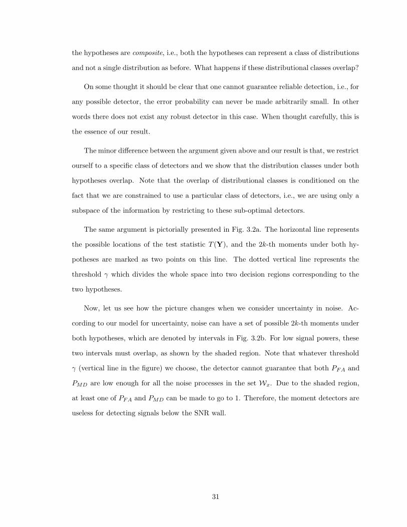
the hypotheses are composite, i.e., both the hypotheses can represent a class of distributions

and not a single distribution as before. What happens if these distributional classes overlap?

On some thought it should be clear that one cannot guarantee reliable detection, i.e., for

any possible detector, the error probability can never be made arbitrarily small. In other

words there does not exist any robust detector in this case. When thought carefully, this is

the essence of our result.

The minor difference between the argument given above and our result is that, we restrict

ourself to a specific class of detectors and we show that the distribution classes under both

hypotheses overlap. Note that the overlap of distributional classes is conditioned on the

fact that we are constrained to use a particular class of detectors, i.e., we are using only a

subspace of the information by restricting to these sub-optimal detectors.

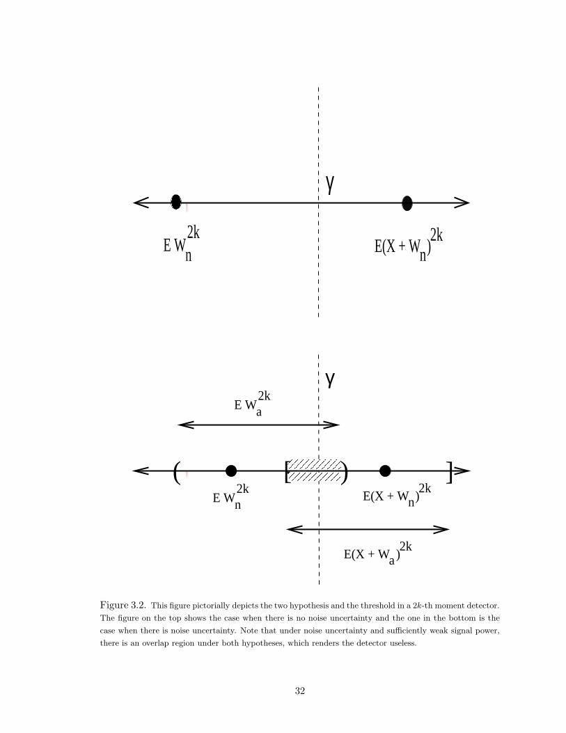
The same argument is pictorially presented in Fig. 3.2a. The horizontal line represents

the possible locations of the test statistic T (Y), and the 2k-th moments under both hy-

potheses are marked as two points on this line. The dotted vertical line represents the

threshold γ which divides the whole space into two decision regions corresponding to the

two hypotheses.

Now, let us see how the picture changes when we consider uncertainty in noise. Ac-

cording to our model for uncertainty, noise can have a set of possible 2k-th moments under

both hypotheses, which are denoted by intervals in Fig. 3.2b. For low signal powers, these

two intervals must overlap, as shown by the shaded region. Note that whatever threshold

γ (vertical line in the figure) we choose, the detector cannot guarantee that both PFA and

PMD are low enough for all the noise processes in the set Wx. Due to the shaded region,

at least one of PFA and PMD can be made to go to 1. Therefore, the moment detectors are

useless for detecting signals below the SNR wall.

31

E W 2kn E(X + W )n

2k

������ γ

E(X + W )n2k

E W n2k

E(X + W )a2k

a2k

E W

��������������������������������������������

γ

( )[ ]

Figure 3.2. This figure pictorially depicts the two hypothesis and the threshold in a 2k-th moment detector.

The figure on the top shows the case when there is no noise uncertainty and the one in the bottom is the

case when there is noise uncertainty. Note that under noise uncertainty and sufficiently weak signal power,

there is an overlap region under both hypotheses, which renders the detector useless.

32

3.6 Approaching the SNR wall

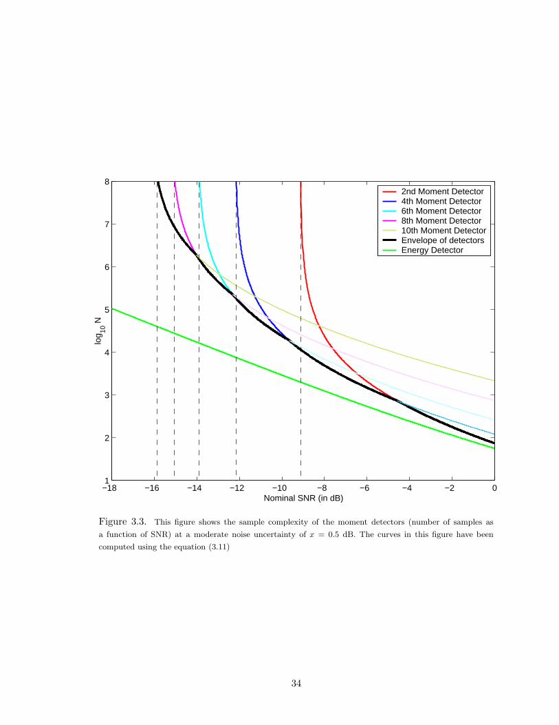
Figure 3.3 shows the sample complexity of moment detectors near the SNR wall. The

green curve shows the sample complexity of the radiometer without noise uncertainty (N =

O(1/SNR2), slope =2). The remaining curves in the figure show the sample complexities

of various moment detectors with noise uncertainty. Recall that the test statistic for a 2k-th

moment detector is given by T (Y) = 1N

∑Ni=1 Y [i]2k, where Y [i] is the i-th received sample.

The values of N we are considering here are very large, in fact larger than the number of

samples required for the radiometer without noise uncertainty. Also, our target probability

of missed detection and false alarm are moderate, i.e., not changing with N . Therefore the

Central Limit theorem is a good approximation here (Note that the error in the central

limit theorem decays as 1/√

N . [3]). Hence, we assume thatT (Y)−NEY 2k

i√Nvar(Yi)

∼ N (0, 1). This

reduces the problem into a standard binary hypothesis testing problem with different mean

under both hypotheses. Therefore, N is given by:

N =

Q−1(PFA)√

(V(Y 2ki )|H0) − Q−1(PD)

√(V(Y 2k

i )|H1)

E(Y 2ki |H1) − E(Y 2k

i |H0)

2

(3.11)

where V(.) stands for the variance operator. Recall that the detector must hit the target

error probabilities uniformly over the whole uncertainty set Wx. Therefore, the sample com-

plexity is dominated by the case when the difference in means (denominator term in (3.11))

in the above equation is minimized.

Thus, the sample complexity required to meet our performance targets uniformly over

the uncertain noise tends to infinity as the SNR tends to SNR(2k)wall. Also note that these

performance curves shift to the left by 10 log k, which verifies that the upper bound obtained

in theorem 1 is very tight.

3.7 Other possible noise uncertainty models

One might argue that the results in section 3.4 arise due to the specific model we used

for noise uncertainty, and that they are not fundamental. In this section, we try to show

33

−18 −16 −14 −12 −10 −8 −6 −4 −2 01

2

3

4

5

6

7

8

Nominal SNR (in dB)

log 10

N

2nd Moment Detector4th Moment Detector6th Moment Detector8th Moment Detector10th Moment DetectorEnvelope of detectorsEnergy Detector

Figure 3.3. This figure shows the sample complexity of the moment detectors (number of samples as

a function of SNR) at a moderate noise uncertainty of x = 0.5 dB. The curves in this figure have been

computed using the equation (3.11)

34

that our model is a minimalist model and any other reasonable noise uncertainty model

will lead to an uncertainty class which includes our uncertainty class. Thus in practice, the

problem will only get worse.

For example, consider the simple case in which the receiver assumes that the noise is

Gaussian, but its estimate of the noise variance is off by some factor, i.e., the receiver

estimates the noise variance to be σ2n, whereas the actual noise variance is σ2

a (σn 6= σa). If

σn > σa then the ratio of their 2k-th moments is(

σn

σa

)2k, which goes to infinity as k → ∞.

Conversely, if σn < σa then(

σn

σa

)2kgoes to zero as k → ∞. Therefore we have shown that

even such a simple case is not included in our noise model. In fact, the above argument

also shows that our uncertainty class Wx includes just one Gaussian, Wn and contains no

other Gaussian random variable.

Motivated by the above example, we propose an alternative noise uncertainty model.

As before, the basic assumptions on the noise remain the same, i.e.,

• We assume that all the noise processes in the uncertainty set to be white.

• Also, we assume that the noise distribution is symmetric, and hence all the odd

moments of the noise random variables are zero.

• Now, suppose that the user estimates the noise to be Gaussian with variance σ2n, i.e.,

Wn ∼ N(0, σ2n). Define the new noise uncertainty set Wx to be the set of all noise

random variables, Wa such that the moments of Wa are all sandwiched between the

corresponding moments of 1α Wn and αWn, i.e., EW 2k

a ∈ [ 1α2k EW 2k

n , α2kEW 2k

n ] where

α = 10(x/10). In other words,

Wx :=

{Wa :

EW 2ka

EW 2kn

∈[

1

α2k, α2k

], Wn ∼ N(0, σ2

n)

}(3.12)

This model is very practical, since in real life, most receivers are not sensitive enough to

be able to differentiate between two Gaussian random variables with very close variances.

Under this model, we now show that there exists a single threshold below which every

35

possible detector fails to detect the signal. Thus, under this model robust detection becomes

absolutely impossible.

For our convenience we rewrite the detection problem under the new noise uncertainty

model

H0 : Y [n] = W [n] n = 1, . . . , N

H1 : Y [n] = X[n] + W [n] n = 1, . . . , N (3.13)

where W ∈ Wx and the remaining setup of the problem is same as in (3.2).

Theorem 2: Consider the detection problem in (3.13). Here we assume that the actual

noise distribution lies in the alternate uncertainty class Wx described in (3.12). Under this

model, we show that there exists an absolute SNR wall (snr∗wall) for any possible robust

detector3. Further, the snr∗wall (the ∗ is used to refer to the fact that it is an absolute wall)

satisfies

snr∗wall = mink>0

snr(2k)wall ≤ α2 − 1 (3.14)

where snr(2k)wall is the snr wall for the 2k-th moment detector and α = 10x/10.

Proof: It is clear that, detection is absolutely impossible if there exists a noise distribu-

tion Wa ∈ Wx, such that Wa = Wn +X or Wn = Wa +X, i.e., either PFA goes to 1 or PMD

goes to 1 respectively. We show that the first condition is satisfied, i.e., Wa := Wn + X.

Observe that

Wa = Wn + X (3.15)

⇔ EW ka = E[Wn + X]k for every k > 0 (3.16)

Since (3.16) is trivially satisfied for k odd, we consider only the case when k is even. Now,

fix k = 2k0. Therefore we must have

EW 2k0a = E[Wn + X]2k0 (3.17)

3Whenever we refer to snrwall in this theorem, we are referring to the wall with respect to the detectionproblem in (3.13) and with the noise uncertainty model given by (3.12)

36

Expanding the above equation, we have

EW 2k0a

EW 2k0n

=

k0∑

i=0

(2k0

2i

)(EW 2k0−2i

n

EW 2kn

)EX2i

=

k0∑

i=0

(2k0

2i

)(1 · 3 · · · (2k0 − 2i − 1)

1 · 3 · · · (2k0 − 1)

)EX2i

σ2in

=

k0∑

i=0

(2k0

2i

)

(2k0 − 2i + 1) · · · · (2k0 − 1)snri

= 1 + k0 · snr + · · · + 1

(2k0 − 1)!!snrk0 (3.18)

Since, Wa ∈ Wx, we must have EfW2k0a

EfW2k0n

≤ α2k0 . Using this bound for the left hand side

of (3.18), we get

α2k0 ≥ 1 + k0 · snr + · · · + 1

(2k0 − 1)!!snrk0 (3.19)

The above equation is exactly the same as in (3.7), and hence we must have

snr ≤ snr(2k0)wall ≤ α2k0 − 1

k0(3.20)

for all k0 ≥ 0. Here the second equation follows from theorem 1, when applied for the case

when α = α2k0 . Hence, detection is impossible iff

Wa = Wn + X

⇔ EW 2k0a = E[Wn + X]2k0 , ∀ k0 > 0

⇔ snr ≤ mink0>0

snr(2k0)wall ≤ min

k0>0

α2k0 − 1

k0

⇔ snr ≤ mink0>0

snr(2k0)wall = α2 − 1

Here the last step is true because of the following fact. The function f(t) := α2t−1t is

monotonically increasing in t ∈ (0,∞) for all α > 1. This can be verified by differentiating

f(t) and showing that the first derivative is strictly positive for t > 0. Hence, we must have

mink0>0

α2k0 − 1

k0= α2 − 1

Therefore, it follows from the definition of snr∗wall that,

snr∗wall = mink0>0

snr(2k0)wall ≤ α2 − 1 (3.21)

which is the required result.

37

Remarks 2: In the proof of the above theorem, we have denoted snr(2k0)wall to be the

solution4 to the equation

α2k0 = 1 + k0 · snr + · · · + 1

(2k0 − 1)!!snrk0 (3.22)

The name coincides with the fact that, this is indeed the location of the SNR wall for the

2k0-th moment detector for the detection problem in (3.2) with the noise uncertainty given

by α = α2k0 (instead of α as before). Now, consider the solution to equation (3.22) as k0

varies. We conjecture that the snr(2k0)wall is monotonically increasing in k0 for any α > 1.

This have been verified numerically for large enough values of k0 and some of the plots are

given in fig. 3.5. If one believes in the above fact then, we must have

mink0>0

snr(2k0)wall = snr

(2)wall

= α2 − 1

Using this in (3.21), we get

snr∗wall = α2 − 1 (3.23)

This gives us an actual closed form expression for the location of the SNR wall under this

alternate model.

In theorem 1 we derived bounds on the SNR walls for the various moment detectors,

under our minimalist noise uncertainty model. There it was shown that the SNR walls

decreases as we check for higher moments and hence the radiometer had the highest value

for SNR wall, given by α − 1. This is equivalent to α2 − 1 in our model, because in the

minimalist model, the uncertainty in the second moment is bounded by α, whereas in this

model the uncertainty in the second moment is bounded by α2−1. Comparing this to (3.23)

we see that, the walls obtained under the alternative noise uncertainty model are greater

than or equal to those obtained for moment detectors in theorem 1. The equality occurs

specifically in the case of the radiometer (see fig. 3.4). This suggests that in real life the

problem of non-detectability can be worse than suggested by the results in theorem 1.

4By solution, we mean the roots of the k0-th degree polynomial given in (3.22). In general this equationwill have k0 roots, but we are interested in the non-negative root only, since snr ≥ 0. However, it is easy toshow that there is a unique non-negative solution to (3.22). Hence the term solution is unambiguous in thiscontext.

38

3.7.1 Discussion

Again, observe that the result in theorem 2 is due to the fact that the distributional

classes under both the hypotheses in (3.13) overlap. The only difference in this case is

that there is overlap irrespective of the detector used, and hence detection is absolutely

impossible below a certain threshold.

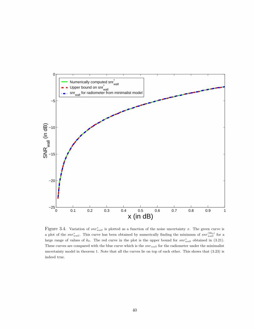
In fig. 3.4 the green curve is a plot of the snr∗wall as a function of the uncertainty in the

noise x. This curve has been obtained by numerically finding the minimum of snr(2k0)wall for a

large range of values of k0. The red curve in the plot is the upper bound for snr∗wall obtained

in (3.21). Both these curves are exactly lying over each other. This shows that (3.23) is

indeed true. Finally, the blue curve in the plot is a plot of the snrwall for the radiometer

obtained in theorem 1. Observe the that the absolute snr∗wall, is exactly equal to the snrwall

for the radiometer, as observed before.

Figure 3.5 plot the solution to (3.22) as a function of k0, for three different values of

x. These figures show that the solution to (3.22) is indeed monotonic in k0 as conjectured.

This shows that the minimum in (3.21) is indeed attained for k0 = 1.

39

0 0.1 0.2 0.3 0.4 0.5 0.6 0.7 0.8 0.9 1−25

−20

−15

−10

−5

0

x (in dB)

SN

Rw

all (

in d

B)

Numerically computed snrwall*

Upper bound on snrwall*

snrwall

for radiometer from minimalist model

Figure 3.4. Variation of snr∗wall is plotted as a function of the noise uncertainty x. The green curve is

a plot of the snr∗wall. This curve has been obtained by numerically finding the minimum of snr

(2k0)wall

for a

large range of values of k0. The red curve in the plot is the upper bound for snr∗wall obtained in (3.21).

These curves are compared with the blue curve which is the snrwall for the radiometer under the minimalist

uncertainty model in theorem 1. Note that all the curves lie on top of each other. This shows that (3.23) is

indeed true.

40

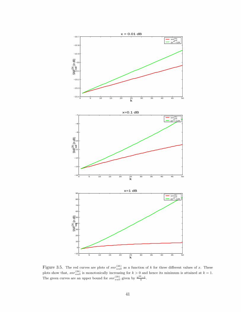
0 5 10 15 20 25 30 35 40 45 50−23.4

−23.3

−23.2

−23.1

−23

−22.9

−22.8

−22.7

k

SNR wa

ll(2

k) (i

n dB

)

x = 0.01 dB

snrwall(2k)

(α2k−1)/k

0 5 10 15 20 25 30 35 40 45 50−14

−13

−12

−11

−10

−9

−8

−7

k

SNR wa

ll(2

k) (i

n dB

)

x=0.1 dB

snrwall(2k)

(α2k−1)/k

0 5 10 15 20 25 30 35 40 45 50−10

0

10

20

30

40

50

60

70

80

90

k

SNR wa

ll(2

k) (i

n dB

)

x=1 dB

snrwall(2k)

(α2k−1)/k

Figure 3.5. The red curves are plots of snr(2k)wall

as a function of k for three different values of x. These

plots show that, snr(2k)wall

is monotonically increasing for k > 0 and hence its minimum is attained at k = 1.

The green curves are an upper bound for snr(2k)wall

given by α2k−1

k.

41

Chapter 4

Finite Dynamic Range and

Quantization

4.1 Introduction

In chapter 3 we motivated the need for taking the uncertainty in noise into considera-

tion while detecting weak zero-mean signals. We proposed two models for the uncertainty

in noise, where we assumed that the noise distribution can lie in a class of distributions

(Wx, Wx). For both these models we discussed the sample complexity of various detectors.

In particular we showed that under the minimalist model discussed in section 3.3, detec-

tion is impossible for moment detectors, at low SNR. Under the alternate model for noise

uncertainty in section 3.7, we showed that robust detection becomes absolutely impossible

for any detector.

Another aspect of practical systems that has not been considered yet is: receivers having

a finite dynamic range limitation. In practice the front ends of receivers have a finite

dynamic range of operation, i.e., the signal coming into the processing unit is bounded in

amplitude. In fact all the receivers have an internal A/D converter following the RF chain

(see fig. 1.2). Therefore, all the detection that the receiver does is based on quantized

versions of the received signal, not the received signal itself. In the previous chapters

42

we ignored these two aspects and assumed that the receiver had infinite precision. It is

intuitively clear that the finite dynamic range assumption and quantization should make

detection harder.

In this chapter, we show that detection is impossible for any detector even under our

minimalist model if the receiver has a finite dynamic range of operation. In particular this

implies that all quantizers with finite number of quantization bins have to face a serious

penalty, which is non-detectability below a certain SNR. However, we consider the 2-

bit quantization case first to motivate the general impossibility result. Through out this

chapter, we work with our minimalist model for noise uncertainty discussed in section 3.31.

4.2 Motivating example: 2-bit quantizer

In section 3.4, we have seen that noise uncertainty renders moment detectors useless if

the SNR falls below a particular threshold. Does this same behavior hold if the signal is

quantized? We analyze a 2-bit quantizer with noise uncertainty. The detection problem

under quantization can be formulated as the following hypothesis testing problem,

H0 : Y [n] = Q(W [n]) n = 1, . . . , N

H1 : Y [n] = Q(X[n] + W [n]) n = 1, . . . , N (4.1)

where Q(.) represents a 2-bit quantizer. Fig. 4.1 shows that bins in a 2-bit quantizer.

Assume that the nominal noise variance is σ2n and the actual noise variance is σ2

a. In this

case, it is easy to verify that the quantizer output is a binary random variable with the

following pmf’s

p(1)1 = 1 − p

(1)0 =

[Q

(d1 −

√P

σa

)+ Q

(d1 +

√P

σa

)]; p

(0)1 = 1 − p

(0)0 = 2Q

(d1

σa

)

1Considering the minimalist model for noise uncertainty is sufficient because of two reasons. Firstly,any impossibility result under this model, will directly imply the corresponding impossibility result in theother model. Secondly, we already showed that under the alternative noise uncertainty model in section 3.7,detection is absolutely impossible even without a finite dynamic range assumption.

43

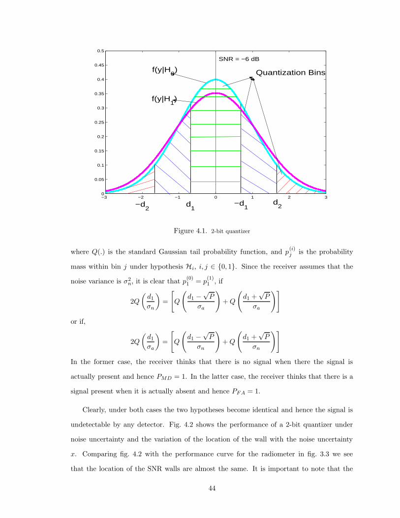
−3 −2 −1 0 1 2 30

0.05

0.1

0.15

0.2

0.25

0.3

0.35

0.4

0.45

0.5

d1

d2−d

1−d2

Quantization Bins f(y|H0)

f(y|H1)

SNR = −6 dB

Figure 4.1. 2-bit quantizer

where Q(.) is the standard Gaussian tail probability function, and p(i)j is the probability

mass within bin j under hypothesis Hi, i, j ∈ {0, 1}. Since the receiver assumes that the

noise variance is σ2n, it is clear that p

(0)1 = p

(1)1 , if

2Q

(d1

σn

)=

[Q

(d1 −

√P

σa

)+ Q

(d1 +

√P

σa

)]

or if,

2Q

(d1

σa

)=

[Q

(d1 −

√P

σn

)+ Q

(d1 +

√P

σn

)]

In the former case, the receiver thinks that there is no signal when there the signal is

actually present and hence PMD = 1. In the latter case, the receiver thinks that there is a

signal present when it is actually absent and hence PFA = 1.

Clearly, under both cases the two hypotheses become identical and hence the signal is

undetectable by any detector. Fig. 4.2 shows the performance of a 2-bit quantizer under

noise uncertainty and the variation of the location of the wall with the noise uncertainty

x. Comparing fig. 4.2 with the performance curve for the radiometer in fig. 3.3 we see

that the location of the SNR walls are almost the same. It is important to note that the

44

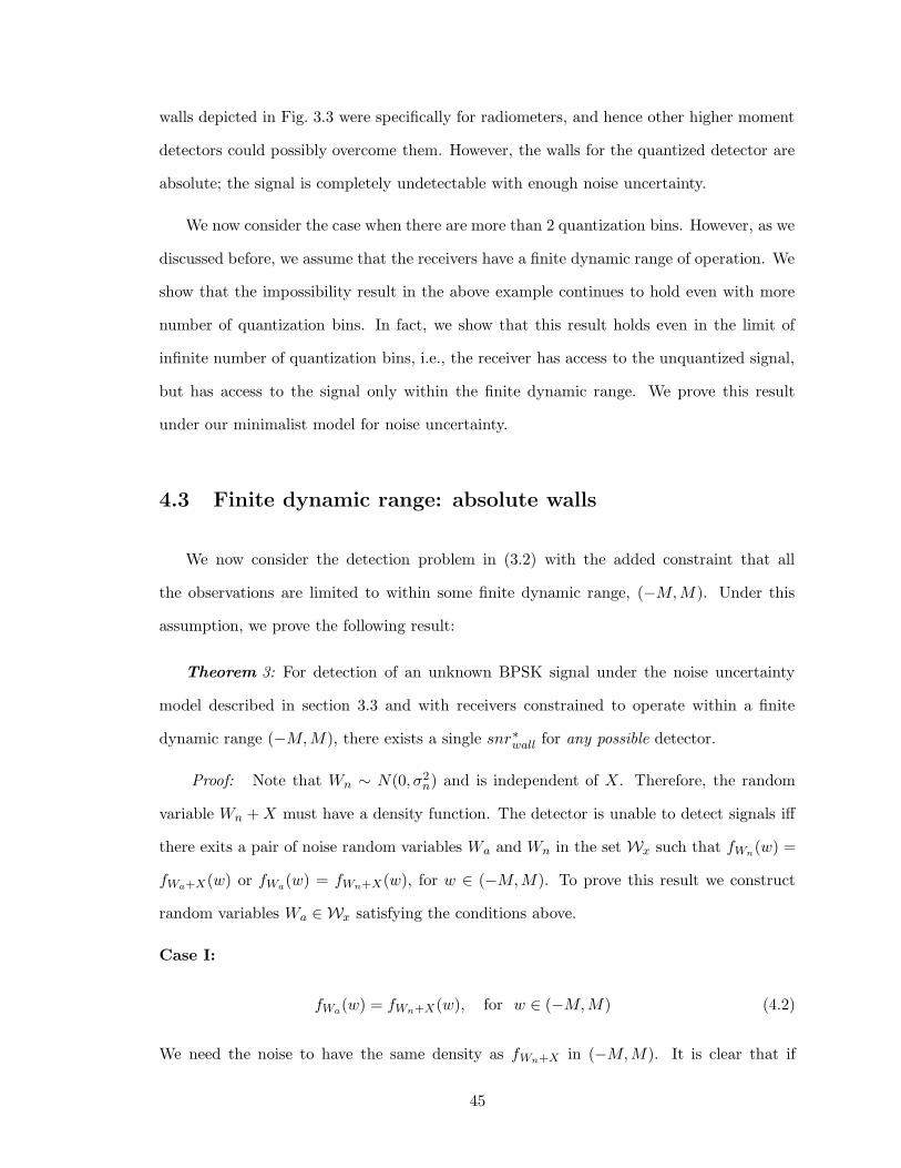
walls depicted in Fig. 3.3 were specifically for radiometers, and hence other higher moment

detectors could possibly overcome them. However, the walls for the quantized detector are

absolute; the signal is completely undetectable with enough noise uncertainty.

We now consider the case when there are more than 2 quantization bins. However, as we

discussed before, we assume that the receivers have a finite dynamic range of operation. We

show that the impossibility result in the above example continues to hold even with more

number of quantization bins. In fact, we show that this result holds even in the limit of

infinite number of quantization bins, i.e., the receiver has access to the unquantized signal,

but has access to the signal only within the finite dynamic range. We prove this result

under our minimalist model for noise uncertainty.

4.3 Finite dynamic range: absolute walls

We now consider the detection problem in (3.2) with the added constraint that all

the observations are limited to within some finite dynamic range, (−M,M). Under this

assumption, we prove the following result:

Theorem 3: For detection of an unknown BPSK signal under the noise uncertainty

model described in section 3.3 and with receivers constrained to operate within a finite

dynamic range (−M,M), there exists a single snr∗wall for any possible detector.

Proof: Note that Wn ∼ N(0, σ2n) and is independent of X. Therefore, the random

variable Wn + X must have a density function. The detector is unable to detect signals iff

there exits a pair of noise random variables Wa and Wn in the set Wx such that fWn(w) =

fWa+X(w) or fWa(w) = fWn+X(w), for w ∈ (−M,M). To prove this result we construct

random variables Wa ∈ Wx satisfying the conditions above.

Case I:

fWa(w) = fWn+X(w), for w ∈ (−M,M) (4.2)

We need the noise to have the same density as fWn+X in (−M,M). It is clear that if

45

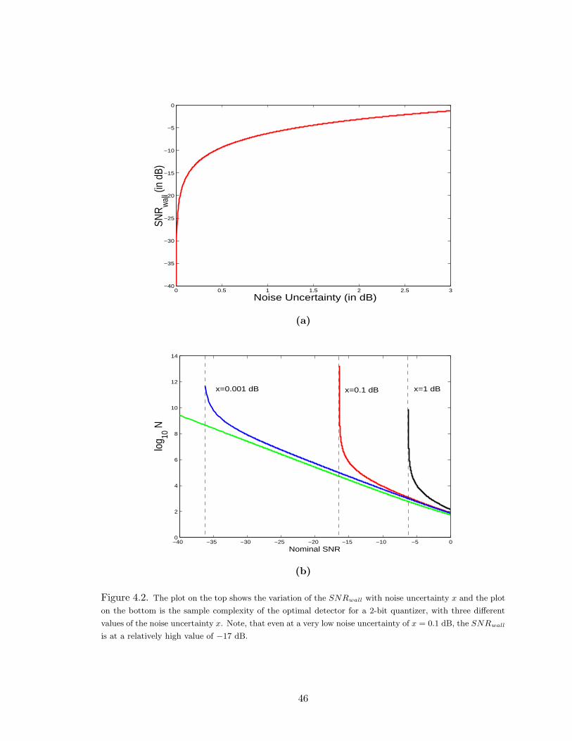
0 0.5 1 1.5 2 2.5 3−40

−35

−30

−25

−20

−15

−10

−5

0

Noise Uncertainty (in dB)

SNR

wal

l (in

dB)

(a)

−40 −35 −30 −25 −20 −15 −10 −5 00

2

4

6

8

10

12

14

Nominal SNR

log 10

N

x=0.1 dB x=1 dBx=0.001 dB

(b)

Figure 4.2. The plot on the top shows the variation of the SNRwall with noise uncertainty x and the plot

on the bottom is the sample complexity of the optimal detector for a 2-bit quantizer, with three different

values of the noise uncertainty x. Note, that even at a very low noise uncertainty of x = 0.1 dB, the SNRwall

is at a relatively high value of −17 dB.

46

we don’t restrict this equality to within this finite dynamic range, then the ratio of the

moments EW 2ka

EW 2kn

→ ∞ as k → ∞ and hence the constructed distribution will fall outside

the uncertainty class. Hence, we equate the densities exactly within the finite dynamic

range and try to reduce the moments by adjusting the density outside the finite dynamic

range. Also, since the signal is very weak, it is safe to assume that |X| � M and hence,

P(|Wa| > M) > P(|Wn| > M). We complete the construction of Wa by defining

fWa(w) = fWn

(w) +λ

2[δ(w − M) + δ(w + M)]

for w ∈ (−M,M)c where the constant λ , P(|Wa| > M)−P(|Wn| > M). Fig. 4.3a illustrates

the noise random variable Wa’s density. Having constructed this random variable, all we

have to check now is whether it actually falls within our uncertainty class, i.e., if EW 2ka

EW 2kn

≤ α.

For this we start off by observing that

EW 2ka

EW 2kn

=1

EW 2kn

[EW 2ka I|Wa|<M + M2k

P(|Wa| = M)

+EW 2ka I|Wa|>M ] (4.3)

Bound the first two terms in (4.3) by

M2k [P(|Wa| < M) + P(|Wa| = M)]

EW 2kn

≤ M2k

EW 2kn

=M2k

(2k − 1)!! σ2kn

−→ 0 (4.4)

as k → ∞. Since the sequence above tends to zero, there exists some kmin such that

EW 2ka I|Wa|<M + M2k

P(|Wa| = M)

EW 2kn

< (α − 1) (4.5)

for all k ≥ kmin. Table 3 lists a few typical values for kmin as a function of M . Now, we

can write the third term in (4.3) as

47

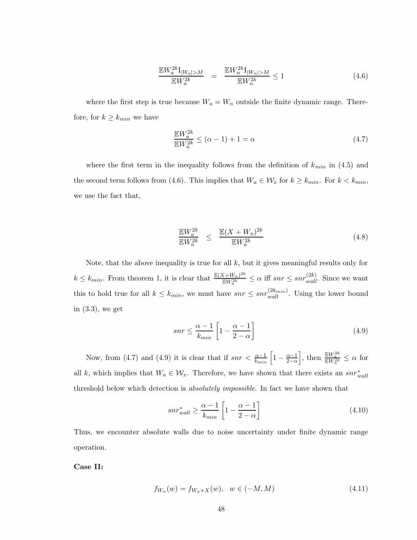
EW 2ka I|Wa|>M

EW 2kn

=EW 2k

n I|Wn|>M

EW 2kn

≤ 1 (4.6)

where the first step is true because Wa = Wn outside the finite dynamic range. There-

fore, for k ≥ kmin we have

EW 2ka

EW 2kn

≤ (α − 1) + 1 = α (4.7)

where the first term in the inequality follows from the definition of kmin in (4.5) and

the second term follows from (4.6). This implies that Wa ∈ Wx for k ≥ kmin. For k < kmin,

we use the fact that,

EW 2ka

EW 2kn

≤ E(X + Wn)2k

EW 2kn

(4.8)

Note, that the above inequality is true for all k, but it gives meaningful results only for

k ≤ kmin. From theorem 1, it is clear that E(X+Wn)2k

EW 2kn

≤ α iff snr ≤ snr(2k)wall. Since we want

this to hold true for all k ≤ kmin, we must have snr ≤ snr(2kmin)wall . Using the lower bound

in (3.3), we get

snr ≤ α − 1

kmin

[1 − α − 1

2 − α

](4.9)

Now, from (4.7) and (4.9) it is clear that if snr < α−1kmin

[1 − α−1

2−α

], then EW 2k

a

EW 2kn

≤ α for

all k, which implies that Wa ∈ Wx. Therefore, we have shown that there exists an snr∗wall

threshold below which detection is absolutely impossible. In fact we have shown that

snr∗wall ≥α − 1

kmin

[1 − α − 1

2 − α

](4.10)

Thus, we encounter absolute walls due to noise uncertainty under finite dynamic range

operation.

Case II:

fWn(w) = fWa+X(w), w ∈ (−M,M) (4.11)

48

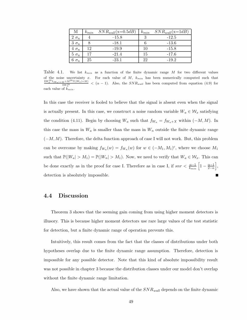
M kmin SNRwall(x=0.5dB) kmin SNRwall(x=1dB)

2 σn 4 –15.8 3 -12.5

3 σn 8 -18.1 6 -13.6

4 σn 12 -19.9 10 -15.8

5 σn 17 -21.4 15 -17.6

6 σn 25 -23.1 22 -19.2

Table 4.1. We list kmin as a function of the finite dynamic range M for two different values

of the noise uncertainty x. For each value of M , kmin has been numerically computed such thatEW

2ka

I|Wa|<M +M2k

P(|Wa|=M)

EW2kn

< (α − 1). Also, the SNRwall has been computed from equation (4.9) for

each value of kmin.

In this case the receiver is fooled to believe that the signal is absent even when the signal

is actually present. In this case, we construct a noise random variable Wa ∈ Wx satisfying

the condition (4.11). Begin by choosing Wa such that fWn= fWa+X within (−M,M). In

this case the mass in Wa is smaller than the mass in Wn outside the finite dynamic range

(−M,M). Therefore, the delta function approach of case I will not work. But, this problem

can be overcome by making fWa(w) = fWn

(w) for w ∈ (−M1,M1)c, where we choose M1

such that P(|Wa| > M1) = P(|Wn| > M1). Now, we need to verify that Wa ∈ Wx. This can

be done exactly as in the proof for case I. Therefore as in case I, if snr < α−1kmin

[1 − α−1

2−α

],

detection is absolutely impossible.

4.4 Discussion

Theorem 3 shows that the seeming gain coming from using higher moment detectors is

illusory. This is because higher moment detectors use rare large values of the test statistic

for detection, but a finite dynamic range of operation prevents this.

Intuitively, this result comes from the fact that the classes of distributions under both

hypotheses overlap due to the finite dynamic range assumption. Therefore, detection is

impossible for any possible detector. Note that this kind of absolute impossibility result

was not possible in chapter 3 because the distribution classes under our model don’t overlap

without the finite dynamic range limitation.

Also, we have shown that the actual value of the SNRwall depends on the finite dynamic

49

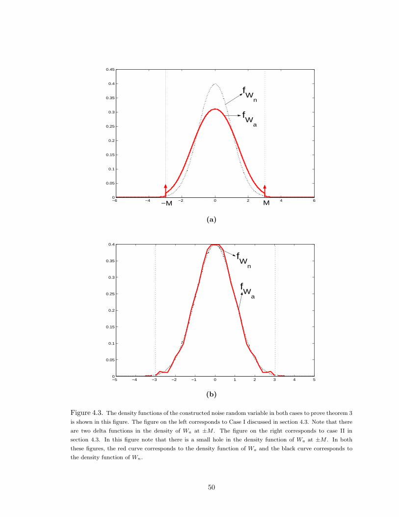
−6 −4 −2 0 2 4 60

0.05

0.1

0.15

0.2

0.25

0.3

0.35

0.4

0.45

−M M

fW

n

fW

a

(a)

−5 −4 −3 −2 −1 0 1 2 3 4 50

0.05

0.1

0.15

0.2

0.25

0.3

0.35

0.4

fW

n

fW

a

(b)

Figure 4.3. The density functions of the constructed noise random variable in both cases to prove theorem 3

is shown in this figure. The figure on the left corresponds to Case I discussed in section 4.3. Note that there

are two delta functions in the density of Wa at ±M . The figure on the right corresponds to case II in

section 4.3. In this figure note that there is a small hole in the density function of Wa at ±M . In both

these figures, the red curve corresponds to the density function of Wa and the black curve corresponds to

the density function of Wn.

50

range M , as shown in table 3. The values in the table suggests that if we build a receiver

with a larger finite dynamic range then the value of the SNRwall decreases. So, it is

important to know how large a value can M take. Lets look into this little more carefully.

Recall that the error term in the Central Limit Theorem, decreases as 1√N

, where N

is the number of independent terms constituting noise. We also discussed that the value

of N is moderate. Further as M increases we are looking into higher and higher values of

the noise, whose probability is equal to the tail probability of the noise. Therefore, it is

important to ask ourselves, if we are confident about the values of noise which have such

a low probability? And the answer to this question is: we are not confident about events

whose probability is comparable to the error term in the CLT. Therefore, it makes sense to

consider only those values of M for which the tail probability of noise O(1/√

N).

Taking the above discussion into consideration, we can easily check that, a reasonable

value for M is 2σn. This implies that the realistic values of the SNRwall are of the order

of −12 dB (see table 3). Hence the limitations proved in this thesis are very realistic.

51

Chapter 5

Comments and Conclusions

In this thesis we have considered fundamental bounds to the detection of the presence or

absence of signals in very low SNR. We discussed the detection problem with and without

considering the uncertainty in noise. In the case when the noise statistics are assumed to be

completely known to the receiver, we showed that detection of zero-mean random signals

without any pilot tones is hard. However, we showed that in the presence of a even a weak

pilot tone the sample complexity of the detector decreases considerably.

We also discussed the problem of detection of sinusoidal signals. We show that, while

imperfect synchronization does cause us to need more samples, the increase in the number

of samples is small compared to the difference in sample complexities of the radiometer and

the matched filter. It is a general feature of coherent detection that processing gain gives

us robustness to a wide range of uncertainties in the system.

While we have assumed that the signal and the noise are independent of each other

and that the noise is white, we assume that we know the distribution of the noise only to

within some uncertain set. Even with a minimalist model of the noise uncertainty, we found

that this implies a fundamental bound on the detectable SNR if we assume that the radio

can only observe the wireless signals and noise to some finite dynamic range. Furthermore,

we showed that detection is absolutely impossible even without this finite dynamic range

limitation if we assume that the noise has a bigger distributional uncertainty class.

52

While our arguments have been focused on the BPSK transmission case, theorem 1, 2

and 3 are not limited to this case. It is not hard to extend our proofs to general zero-mean

signal constellations with low signal amplitude. In addition, we believe that these results

reflect the generic difficulty of the low SNR signal detection problem and not peculiarities

of our model. For example, let us consider the case when the signal is no longer white.1 In

that case, it is possible to use feature detectors (see [8], [9]) to exploit the colored nature

of the signal. However, in such cases, it will also be natural to consider our noise as being

only approximately white. After all, it reflects the sum of many different physical sources

of undesired signals, not all of which are white! For example in real life, mixers in receivers

are non-linear and hence actual signals from other bands are also mixed into the original

signal. For low enough SNR, we suspect the structure brought by signals from other bands

will be indistinguishable from the uncertain low level structure of the noise.

These sorts of fundamental bounds make us further appreciate the usefulness and ro-

bustness of the coherent signal processing possible whenever the primary signal has known

frequency specific training data or pilot tones. Coherent processing enables us to take long

averages that bring the SNR up to a reasonable value for detection.

Finally, we must point out that throughout this thesis we have ignored the presence

of fading, which is inherent in most of the wireless channels [27]. One expects that the

effect of channel fading should not make the problem of detection any easier. Since most

of our results are impossibility results, the presence of fading does not make a qualitative

difference to the nature of our results.

However, we must be cautious in ignoring the effect of fading in the case of coherent

detection, especially in the problem of detecting a weak pilot signal. It is possible that

the presence of channel fading can make it very hard for detecting pilot signals. Factors

like, Doppler shift, pilot tones from multiple primary users, multi-path fading can have an

adverse effect on these weak pilot tones and can make it impossible to detect them. We

suspect that, a careful analysis of this problem might lead to similar impossibility results

1This just means that we are not going to sample it faster than the Nyquist rate.

53

for the problem of detection of weak pilot signals. However, the position of these new SNR

walls might be lower than the ones for non-coherent detection obtained in this thesis.

54

References

[1] T. Bayes, “An essay toward solving a problem in the doctrine of chances,” Phil. Trans. Roy. Soc.,vol. 53, pp. 370–418, 1763.

[2] R. W. Broderson, A. Wolisz, D. Cabric, S. M. Mishra, and D. Willkomm, “(2004) white paper:Corvus: A cognitive radio approach for usage of virtual unlicensed spectrum.” [Online]. Available:http://bwrc.eecs.berkeley.edu/Research/MCMA/CR White paper final1.pdf

[3] R. Durrett, Probability: Theory and Examples, 3rd ed. Belmont: Duxbury Press, 2004.

[4] A. H. El-Sawy and V. D. VandeLinde, “Robust detection of known signals,” IEEE Trans. Inform.

Theory, vol. 23, pp. 222–229, March 1977.

[5] FCC, “Et docket no. 03-237,” November 2003. [Online]. Available: http://hraunfoss.fcc.gov/edocs public/attachmatch/FCC-03-289A1.pdf

[6] ——, “Et docket no. 03-322,” December 2003. [Online]. Available: http://hraunfoss.fcc.gov/edocspublic/attachmatch/FCC-03-322A1.pdf

[7] R. A. Fisher, “On the mathematical foundations of theoretical statistics,” Phil. Trans. Roy. Soc., vol.A 222, pp. 309–368, 1922.

[8] W. A. Gardner, “Signal interception: Performance advantages of cyclic-feature detectors,” IEEE Trans.

Commun., vol. 40, pp. 149–159, January 1992.

[9] ——, “Signal interception: A unifying theoretical framework for feature detection,” IEEE Trans. Com-

mun., vol. 36, pp. 897–906, August 1998.

[10] C. F. Gauss, Theoria Combinationis Observationum Erroribus Minimis Obnoxia. Germany: Dieterich:Gottingen, 1823.

[11] N. Hoven, “On the feasibility of cognitive radio,” Master’s thesis, University of California, Berkeley,2005.

[12] N. Hoven and A. Sahai, “Power scaling for cognitive radio,” in WirelessCom Symposium on Emerging

Networks, Technologies and Standards, June 2005.

[13] P. J. Huber, “Robust estimation of a location parameter,” Ann. Math. Statist., vol. 35, pp. 73–101,March 1964.

[14] ——, “A robust version of the probability ratio test,” Ann. Math. Statist., vol. 36, pp. 1753–1758,December 1965.

[15] T. Kailath and V. Poor, “Detection of stochastic processes,” IEEE Trans. Inform. Theory, vol. 44, pp.2230–2259, October 1998.

[16] S. A. Kassam and J. B. Thomas, “Asymptotically robust detection of a known signal in contaminatednongaussian noise,” IEEE Trans. Inform. Theory, vol. 22, pp. 22–26, January 1976.

[17] S. M. Kay, Fundamentals of statistical signal processing: Detection theory. Printice Hall PTR, 1998,vol. 2.

[18] R. D. Martin and S. C. Schwartz, “Robust detection of a known signal in nearly gaussian noise,” IEEE

Trans. Inform. Theory, vol. 17, pp. 50–56, January 1971.

[19] D. Middleton, “On the detection of stochastic signals in additive normal noise - part i,” IEEE Trans.

Inform. Theory, vol. 3, pp. 86–121, June 1957.

[20] I. J. Mitola, “Software radios: Survey, critical evaluation and future directions,” IEEE Aerosp. Electron.

Syst. Mag, vol. 8, pp. 25–36, April 1993.

[21] J. Neyman and E. Pearson, “On the problem of the most efficient tests of statistical hypotheses,” Phil.

Trans. Roy. Soc., vol. A 231, no. 9, pp. 492–510, 1933.

[22] R. Price and N. Abramson, “Detection theory,” IEEE Trans. Inform. Theory, vol. 7, pp. 135–139, July1961.

[23] A. Sahai, N. Hoven, and R. Tandra, “Some fundamental limits on cognitive radio,” in Forty-Second

Allerton Conference on Communication, Contol and Computing, September 2004.

[24] C. E. Shannon, “A mathematical theory of communication,” Bell Sys. Tech. J., vol. 27, pp. 379–423,623–656, 1948.

[25] D. Slepian, “Some comments on the detection of gaussian signals in gaussian noise,” IEEE Trans.

Inform. Theory, vol. 4, pp. 65–68, June 1958.

[26] A. Sonnenschein and P. M. Fishman, “Radiometric detection of spread-spectrum signals in noise ofuncertain power,” IEEE Trans. Aerosp. Electron. Syst., vol. 28, pp. 654–660, July 1992.

55

[27] D. Tse and P. Vishwanath, Fundamentals of wireless communications. Cambridge University Press,2005.

[28] J. W. Tukey, A survey of sampling from contaminated distributions, ser. Essays in Honor of HaroldHotelling, I. Olkin et al, Stanford and Calif., Eds. Stanford Univ. Press, 1960.

[29] H. Urkowitz, “Energy detection of unknown deterministic signals,” Proc. IEEE, vol. 55, pp. 523–531,1967.

56

Appendix A

Appendix: Sample complexity of

BPSK detector

A.0.1 Detection Performance using the Central Limit Theorem

From (2.14), we have

T (Y) =

N−1∑

i=0

ln

[exp

√PY [i]

σ2+ exp

−√

PY [i]

σ2

]

=:N−1∑

i=0

Yi (A.1)

where

Yi := ln

[exp

√PY [i]

σ2+ exp

−√

PY [i]

σ2

]

and

Zi :=

[exp

√PY [i]

σ2+ exp

−√

PY [i]

σ2

]

Thus,Yi = f(Zi) = lnZi

Observe that Yi, i = 0, 1, . . . , N−1 are independent, identically distributed random variablesand the test statistic T (Y) is a sum of independent, identically distributed random variables(see (A.1)). Hence by the central limit theorem for large N ,

T (Y) − Nmi√N

∼ N(0, σ2

i

)

where mi := E(Yi) and σ2i = Var(Yi). In order to use the CLT we will have to find the

mean and variance of the random variable Yi. Unfortunately, we cannot express mi and σ2i

in closed form. Hence we use the Taylor series expansion of the function Yi = f(Zi) at themean of Zi.

Yi = f [µZi] + [Zi − µZi

]f ′(Zi)|µZi+

1

2[Zi − µZi

]2f ′′(Zi)|µZi+ . . .

57

where E(Zi) =: µZi. We use only the first order terms to get

mi ≈ f(µZi)

σ2i ≈

[f ′(Zi)|µZi

]2V ar(Zi) (A.2)

Using the above approximations we evaluate the mean and variance of Yi under both thehypothesis.

1. Under H0:

Yi = ln

[exp

√PY [i]

σ2+ exp

−√

PY [i]

σ2

]

where Y [i] ∼ N (0, σ2). Thus, using (A.2) we have

E(Yi) = mi ≈ f(µZi)

= ln

(E

[exp

√PY [i]

σ2+ exp

−√

PY [i]

σ2

])

= ln

(2E

[exp

√PY [i]

σ2

])

= ln

(2 exp(

1

2

d2

σ2)

)

= ln(2 exp(

snr

2))

(A.3)

Again from (A.2), we have

V ar(Yi) = σ2i ≈

[f ′(Zi)|µZi

]2V ar(Zi)

=V ar(Zi)

µZi

2

We know thatV ar(Zi) = E(Z2

i ) − E2(Zi)

Hence, we evaluate each term of the above equation separately.

E(Z2i ) = E

(

exp

√PY [i]

σ2+ exp

−√

PY [i]

σ2

)2

= E

[exp

2√

PY [i]

σ2+ exp

−2√

PY [i]

σ2+ 2

]

= 2 + 2E

[exp

2√

PY [i]

σ2

]

= 2 + 2 exp(2snr)

Therefore,

V ar(Zi) = 2 + 2 exp(2snr) − 4 exp(snr) (From (A.3))

= 2 [exp(snr) − 1]2

58

Hence,

V ar(Yi) = σ2i ≈ 2 [exp(snr) − 1]2

µZi

2

and,

σi ≈√

2 [exp(snr) − 1]

µZi

=[exp(snr) − 1]√

2 exp( snr2 )

≈ 1√2

[1 + snr − snr]

1 + snr2

≈ snr√2

(A.4)

Here we have used the fact that, at low snr, i.e., when snr � 1, exp(snr) ≈ 1 + snr

2. Under H1:

Yi = ln

[exp

√PY [i]

σ2+ exp

−√

PY [i]

σ2

]

where Y [i] ∼ N (ai, σ2) and ai ∼ Bernoulli(1/2). Thus, using the Taylor series ap-

proximation in (A.2) we have

E(Yi) = mi ≈ f(µZi)

= ln

(E

[exp

√PY [i]

σ2+ exp

−√

PY [i]

σ2

])

= ln

(E

[exp

√P (ai + x[i])

σ2+ exp

−√

P (ai + x[i])

σ2

])

= ln

(E

[exp(

√Pai

σ2)

]E

[exp(

√P ˜˜[i]x

σ2)

]+ E

[exp(

−√

Pai

σ2)

]E

[exp(

−√

P x[i]

σ2)

])

= ln

(2

[(exp(snr) + exp(−snr))

2

]exp(

snr

2)

)

= ln

[(exp(snr) + exp(−snr))

2

]+ ln

[2 exp(

snr

2)]

(A.5)

Where x[i] ∼ N (0, σ2) and independent of ai and hence we justify writing the expec-tation as a product in the 4th step of the above series of equations.

We now need to calculate the Variance of Yi. As before we have

V ar(Yi) ≈[f ′(Zi)|µZi

]2V ar(Zi)

=V ar(Zi)

µZi

2

andV ar(Zi) = E(Z2

i ) − E2(Zi) (A.6)

59

So, we evaluate each term in the above expression.

E(Z2i ) = E

(

exp

√PY [i]

σ2+ exp

−√

PY [i]

σ2

)2

= E

[exp

2√

PY [i]

σ2+ exp

−2√

PY [i]

σ2+ 2

]

= 2 + 2E

[exp

2√

PY [i]

σ2

]

= 2 + 2E

[exp

2d(ai + x[i])

σ2

]

= 2 + 2E

[exp

(2dai

σ2

)exp

(2dx[i]

σ2

)]

= 2 + 2E

[exp

(2dai

σ2

)]E

[exp

(2dx[i]

σ2

)]

= 2 + 2

[exp(2snr) + exp(−2snr)

2

]exp(2snr)

= 2 + [exp(2snr) + exp(−2snr)] exp(2snr) (A.7)

Substituting (A.7) in (A.6) we get

V ar(Zi) = 2 + [exp(2snr) + exp(−2snr)] exp(2snr) − E2(Zi)

= 2 + [exp(2snr) + exp(−2snr)] exp(2snr) −[exp(snr) + exp(−snr)]2 exp(snr)

(From (A.5))

= 3 + exp(4snr) − exp(3snr) − exp(−snr) − 2 exp(snr)

Therefore,

V ar(Yi) ≈ 3 + exp(4snr) − exp(3snr) − exp(−snr) − 2 exp(snr)

[exp(snr) + exp(−snr)]2 exp(snr)

Since we are concerned with the low snr scenario, we again use the fact that, whensnr � 1, exp(snr) ≈ 1 + snr and simplify the above expression to obtain:

V ar(Yi) ≈ snr2

⇒√

V ar(Yi) ≈ snr (A.8)

Finally, to summarize we define, mk := E(Yi|Hk) for k = 0, 1 and all i = 0, 1, . . . , N − 1.Similarly define, σk :=

√V ar(Yi|Hk) for k = 0, 1. Thus, summarizing the results of the

previous two section:

m0 ≈ ln[2 exp(

snr

2)]

m1 ≈ ln

[exp(snr) + exp(−snr)

2

]+ ln

[2 exp(

snr

2)]

σ0 = O(snr)

σ1 = O(snr) (A.9)

60

From the above equations we also have

m1 − m0 = ln

[exp(snr) + exp(−snr)

2

]

≈ snr2 (A.10)

For snr � 1. Now, we apply the use these expressions to derive the detection performance.We have

PFA = Pr(T (Y) > γ′|H0

)

= Pr

(T (Y − Nm0)√

Nσ0

>γ′ − Nm0√

Nσ0

|H0

)

= Q

(γ′ − Nm0√

Nσ0

)(By CLT)

Simplifying this,γ′ =

√Nσ0Q

−1(PFA) + Nm0 (A.11)

Similarly,

PD = Pr(T (Y) > γ′|H1

)

= Pr

(T (Y − Nm1)√

Nσ1

>γ′ − Nm1√

Nσ1

|H1

)

= Q

(γ′ − Nm1√

Nσ1

)(By CLT)

andγ′ =

√Nσ1Q

−1(PD) + Nm1 (A.12)

Eliminating γ ′ from (A.11) and (A.12) we have,

N =

[σ0Q

−1(PFA) − σ1Q−1(PD)

m1 − m0

]2

Using (A.9) and (A.10) in the above equation we have,

N ≈[snrQ−1(PFA) − snrQ−1(PD)

snr2

]2

=[Q−1(PFA) − Q−1(PD)

]2snr−2

≈ snr−2 (A.13)

61