calculating the detection limits of chamber-based soil ... parkin et al... · calculating the...

705

Renewed interest in quantifying greenhouse gas emissions from soil has led to an increase in the application of chamber-based fl ux measurement techniques. Despite the apparent conceptual simplicity of chamber-based methods, nuances in chamber design, deployment, and data analyses can have marked eff ects on the quality of the fl ux data derived. In many cases, fl uxes are calculated from chamber headspace vs. time series consisting of three or four data points. Several mathematical techniques have been used to calculate a soil gas fl ux from time course data. Th is paper explores the infl uences of sampling and analytical variability associated with trace gas concentration quantifi cation on the fl ux estimated by linear and nonlinear models. We used Monte Carlo simulation to calculate the minimum detectable fl uxes (α = 0.05) of linear regression (LR), the Hutchinson/Mosier (H/M) method, the quadratic method (Quad), the revised H/M (HMR) model, and restricted versions of the Quad and H/M methods over a range of analytical precisions and chamber deployment times (DT) for data sets consisting of three or four time points. We found that LR had the smallest detection limit thresholds and was the least sensitive to analytical precision and chamber deployment time. Th e HMR model had the highest detection limits and was most sensitive to analytical precision and chamber deployment time. Equations were developed that enable the calculation of fl ux detection limits of any gas species if analytical precision, chamber deployment time, and ambient concentration of the gas species are known.

Calculating the Detection Limits of Chamber-based Soil Greenhouse Gas Flux Measurements

T. B. Parkin,* R. T. Venterea, and S. K. Hargreaves

Over the past two decades, scientifi c publi-cations on greenhouse gas (GHG) emissions from soil have increased exponentially. A cursory search of

papers using key words “greenhouse gas,” “emissions,” and “soil” (Web of Science) revealed 145 papers over the period 1990 to 2000, 217 papers over the period 2000 to 2004, 674 papers over the period 2004 to 2009, and 365 papers in 2010 to 2011. Chamber methods are a common technique to measure trace gas fl uxes from soil. Th ey are low cost and are suitable for scientifi c studies because they allow for treatment replication. However, the apparent simplicity of the soil chamber approach belies the complexities associated with obtaining accurate fl ux estimates. Rochette and Eriksen-Hamel (2008) developed criteria for assessing the reliability of chamber-based fl ux estimates based on 16 characteristics, including chamber design, deployment time, gas sampling and measurement procedures, and data analyses. From an analysis of 356 studies, they concluded that the qual-ity of approximately 60% of these studies was either low or very low regarding the accuracy of the chamber fl uxes reported. A primary issue highlighted by the Rochette and Eriksen-Hamel study was the bias associated with fl ux estimates induced by the fl ux calculation method.

It is generally recognized that when chambers are placed on the soil surface, conditions are altered so that the fl ux of gas is aff ected. Buildup of gas in the chamber headspace and soil pores reduces the diff usive fl ux of gas from the soil surface when the chamber is in place, resulting in chamber headspace gas con-centrations vs. time data that are nonlinear (Hutchinson and Mosier, 1981; Livingston and Hutchinson, 1995). Application of linear regression to such data results in fl uxes that underes-timate the actual predeployment fl ux (Hutchinson and Mosier, 1981; Livingston and Hutchinson, 1995; Healy et al., 1996; Livingston et al., 2006; Rochette and Bertrand, 2007; Venterea and Baker, 2008; Venterea, 2010).

Abbreviations: DT, chamber deployment time; GC, gas chromatograph; GHG,

greenhouse gas; H/M, Hutchinson/Mosier; HMR, revised Hutchinson/Mosier; LR,

linear regression; MDL, minimum detection limit; NDFE, non–steady-state diff usive

fl ux estimator; Quad, quadratic; rH/M, restricted Hutchinson/Mosier; rQuad,

restricted quadratic.

T.B. Parkin, USDA–ARS, National Lab. for Agriculture and the Environment, 2110

University Blvd., Ames, IA 50011; R.T. Venterea, USDA–ARS, Soil and Water Research

Management Unit, 1991 Upper Buford Cir., 439 Borlaug Hall, St., Paul, MN 55108;

S.K. Hargreaves, Dep. of Ecology, Evolution and Organismal Biology, Iowa State

Univ., 253 Bessey Hall, Ames, IA, 50011. Mention of trade names or commercial

products in this article is solely for the purpose of providing specifi c information

and does not imply recommendation or endorsement by the U.S. Department of

Agriculture. The USDA is an equal opportunity provider and employer. Assigned to

Associate Editor Martin H. Chantigny.

Copyright © 2012 by the American Society of Agronomy, Crop Science Society

of America, and Soil Science Society of America. All rights reserved. No part of

this periodical may be reproduced or transmitted in any form or by any means,

electronic or mechanical, including photocopying, recording, or any information

storage and retrieval system, without permission in writing from the publisher.

J. Environ. Qual. 41:705–715 (2012)

doi:10.2134/jeq2011.0394

Supplemental data fi le is available online for this article.

Freely available online through the author-supported open-access option.

Received 12 Oct. 2011.

*Corresponding author ([email protected]).

© ASA, CSSA, SSSA

5585 Guilford Rd., Madison, WI 53711 USA

Journal of Environmental QualityATMOSPHERIC POLLUTANTS AND TRACE GASES

TECHNICAL REPORTS

706 Journal of Environmental Quality

Th ere have been several mathematical algorithms applied to correct for this diff usion eff ect. Hutchinson and Mosier (1981) developed an equation that uses three sample points collected at equal time intervals (Hutchinson/Mosier [H/M] method). Th e quadratic procedure described by Wagner et al. (1997) involves fi tting a quadratic equation to the concentration vs. time data (Quad method). Th e fl ux is then computed as the fi rst deriva-tive of the quadratic equation at time zero. Pedersen et al. (2001) developed a stochastic diff usion model that is an extension of the H/M method and does not require data points determined at equal time intervals and can accommodate more than three data points. Th e non-steady-state diff usive fl ux estimator (NDFE) developed by Livingston et al. (2006) is a three-parameter model in which the predeployment fl ux can be derived from concen-tration vs. time data by nonlinear regression. Recently, Pedersen et al. (2010) developed a technique designated as the revised Hutchinson/Mosier (HMR) model, which is a modifi cation of the H/M technique to account for horizontal gas diff usion and chamber leaks. Similar to the Pedersen et al. (2001) stochastic model, the Quad method, and the NDFE model, the HMR technique can be used with data sets of three or more points. Th e common goal of all of these techniques is elimination of the bias associated with the assumption that the concentration vs. time data are linear. However, there are statistical properties other than bias associated with estimators.

Th e variance associated with diff erent fl ux estimation meth-ods is infl uenced by the variability in the concentration vs. time data. Th is variance aff ects the minimum detection limit associ-ated with a given fl ux calculation technique. In this study, we used Monte Carlo sampling to determine the positive and nega-tive fl ux detection limits associated with diff erent fl ux calculation procedures at a Type I error rate of 0.05. Th ese assessments were done over a range of analytical precisions and chamber deploy-ment times and for two sampling intensities (three or four points per fl ux data set). For the purposes of illustration, in this work we use N2O as an example. We also scaled the N2O results so they would be gas species independent. Furthermore, the minimum detectable fl uxes of each fl ux calculation method for other gas species can be determined if analytical precision, chamber DT, and ambient concentration of the gas are known.

Materials and MethodsSampling Precision of Gas Chromatography

Sampling and analytical precisions of the gas chromato-graphic measurements of N2O, CH4, and CO2 at ambient con-centrations were determined by calculating the SDs and CVs from 35 air samples. Air samples (11.4 mL) were collected in a 10-mL polypropylene syringe and injected into evacuated glass serum vials (empty volume ~10.5 mL), which were capped with gray butyl rubber stoppers (Voigt Global). In the laboratory, the samples were analyzed for N2O, CH4, and CO2 using a gas chromatograph (GC) (model 8610C, SRI Instruments). An autosampler similar in design to that described by Arnold et al. (2001) was connected to the GC to facilitate sample injection via a sample valve with a 1.0-mL sample loop. Gas species sepa-ration was accomplished with stainless steel columns (0.3175 cm diameter × 74.54 cm long) packed with Haysep D and contained in the GC column oven operated at 50°C. Nitrous

oxide was detected with an electron capture detector operated at 325°C. Methane and CO2 were measured with a methanizer interfaced with a fl ame ionization detector operated at 350°C. Th e carrier gas (N2) fl ow rate through the column was 20 mL min−1. Certifi ed standard gases (±5%) were obtained from Scott Specialty Gas and used to generate the relationships between detector voltage output and gas concentrations. Precisions of the gas chromatographic analyses of N2O, CH4, and CO2 were determined by computing the means and standard deviations of the 35 measurements of each gas species in air. Precision of mea-surement of each gas species is expressed as its CV as proscribed by American Public Health Association (1985). Normality of the distributions of the concentrations of the gas species and of the distributions of calculated fl uxes was determined by the Kolmogorov Smirnov test. Symmetry of the distributions was assessed by calculating skewness and by examining the trends exhibited by the midsummaries of the ordered fl uxes as described by Emerson and Stoto (1983). It was important to determine the distributional properties of the GHGs of interest to guide con-struction of the populations for the Monte Carlo samplings.

Monte Carlo Simulations: Limit of Detection

of Gas FluxesFlux determinations using non–steady-state soil chamber

techniques typically rely on discrete samples collected from a chamber headspace over a fi xed time interval. Th e fl ux is then cal-culated by determining the change in gas concentration vs. time relationship by a curve fi tting procedure. However, sampling and analytical error contribute to uncertainty in the gas concentration measurements at each point in time. For example, Fig. 1 shows hypothetical N2O fl ux determinations based on measurement of

Fig. 1. Illustration of how a Type I error is manifested. An apparent positive fl ux (A) or a negative fl ux (Fig. 1B) is calculated when no actual change in headspace gas concentration is occurring.

www.agronomy.org • www.crops.org • www.soils.org 707

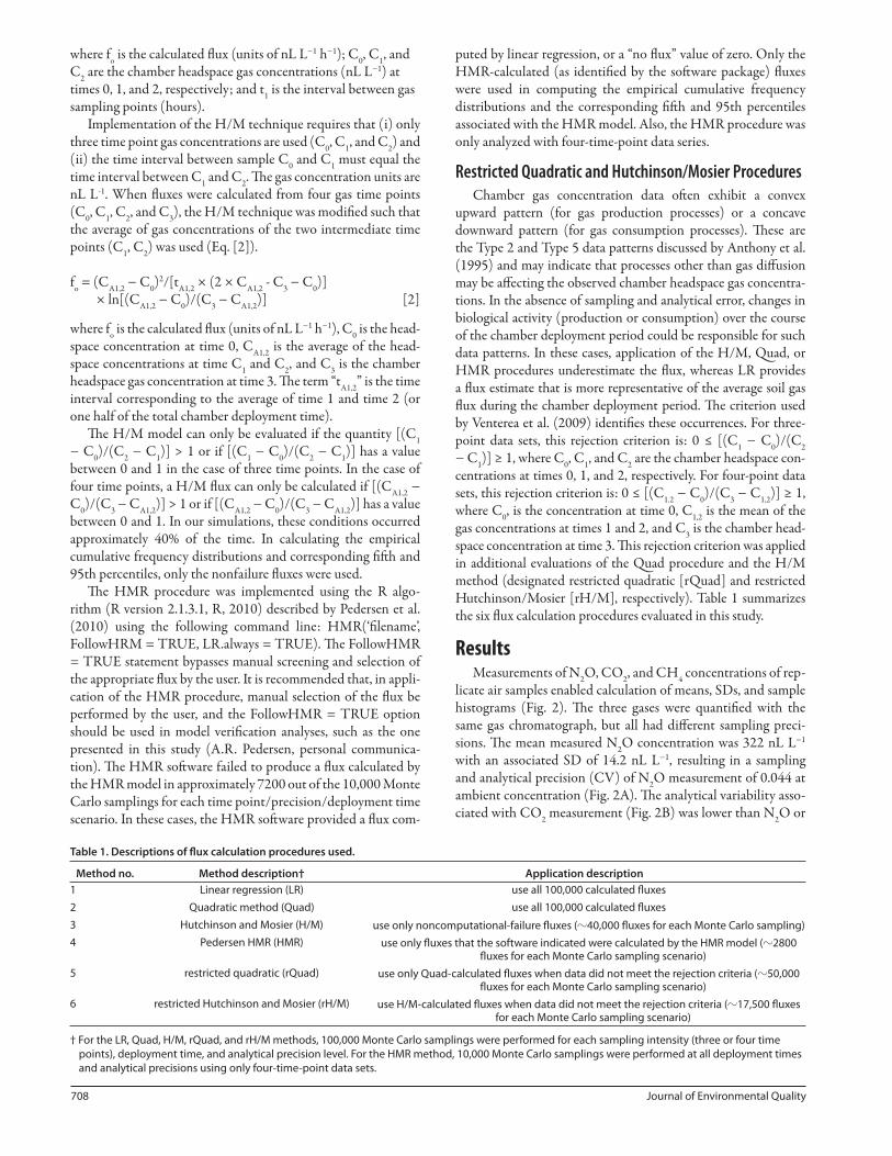
chamber headspace gas concentrations at three points in time. Th e data points in Fig. 1 show the measured concentrations at each time, and the bell-shape curves represent the fact that each discrete measurement is drawn from a population defi ned by the mean concentration and the measurement variability. In these examples, although the mean chamber headspace N2O concentra-tion does not change over time (it remains constant at 322 nL L-1 [ppb] as represented by the dashed horizontal line), sampling and analytical variability (as represented by the bell-shaped normal distribution curves) result in potential gas measurements that could indicate an apparent positive or negative fl ux. Reporting these apparent positive or negative fl uxes as signifi cant would be committing a Type I error (i.e., rejecting the null hypothesis [H0; fl ux = 0]) when in fact the fl ux does equal 0).

Th e impacts of sampling and analytical variability on the fl ux threshold value associated with a Type I error rate of 0.05 (i.e., the fl ux detection limit) for the diff erent methods were evalu-ated by constructing gas concentration distributions with diff er-ent SDs (i.e., diff erent sampling and analytical precisions) and by sampling these distributions using Monte Carlo analysis. For these evaluations, scenarios were established whereby distribu-tions corresponding to trace gas concentration measurements at distinct points in time were generated (Fig. 2). In these analy-ses, the means of the distributions of each gas remained constant (i.e., no change in trace gas concentration over time); therefore, the underlying fl ux is 0.

Th e Monte Carlo simulations were performed by generat-ing variates from the unit normal distribution (mean, 0; SD, 1) using the Box-Muller algorithm (Box and Muller, 1958) and the Microsoft Excel @RAND function. Normal variates from dis-tributions corresponding to trace gas concentrations were then generated by multiplying the unit normal variate by the SD of the target population and adding the mean of the target population.

Samples were selected from the distributions at each time point, and a fl ux was calculated using several calculation tech-niques (described below). For all the scenarios, the means of the distributions were the same, but diff erent scenarios had diff er-ent SDs to represent diff erent sampling and analytical precisions. For each scenario, 100,000 Monte Carlo simulations were run, and 100,000 fl ux estimates were calculated using each of the calculation methods (except the for HRM method). Due to the computationally intensive nature of the nonlinear regres-sion used to evaluate the HMR model, only 10,000 Monte Carlo simulations were performed for the HMR technique over the ranges of analytical precisions and sampling intensities. In some cases, the populations of fl uxes generated by the Monte Carlo simulations were signifi cantly diff erent from the normal distribution, so empirical cumulative probability density func-tions were constructed. Th ese were done by ranking the fl uxes in ascending order. Th e probability associated with each fl ux measurement was then calculated by dividing its rank number by the total number of fl uxes represented in the cumulative distri-bution. From each cumulative probability density function, the fl ux corresponding to the 95th percentile was deemed to be the detection limit of the positive fl uxes, and the fl ux correspond-ing to the fi ft h percentile was deemed to be the detection limit of negative fl uxes (the cumulative probability density functions were approximately symmetrical around zero). Th ese 95th and

fi ft h percentile fl uxes represent the 5% Type I error threshold fl uxes at the positive and negative tails of the distributions.

Th e scenarios were run at sampling and analytical precisions (CVs) of 0.01, 0.02, 0.03, 0.04, 0.05, 0.06, 0.08, 0.10, and 0.12. Because chamber deployment time and chamber sampling fre-quency also aff ect the calculated fl ux, simulations were run at simulated chamber deployment times of 0.1, 0.25, 0.5, 0.75, 1.0, and 2.0 h using both three and four equally spaced time points for each CV level. For illustrative purposes, the populations used in each Monte Carlo sampling scenario were generated to repre-sent N2O emissions in that they had means of 320 nL L−1, which correspond to the ambient atmospheric air N2O concentration. However, the results obtained were scaled and thus are appli-cable to other gas species with diff ering ambient concentrations.

Flux Calculation ProceduresTh e fl ux calculation methods evaluated were linear regression

(LR), the Hutchinson and Mosier (1981) (H/M) technique, the quadratic method (Quad) (Wagner et al., 1997), and the HMR procedure (Pedersen et al., 2010). Linear regression and Quad fl uxes were calculated using the Microsoft Excel LINEST func-tion (Venterea et al., 2009). Th e H/M method was implemented as described in Eq. 1 when three gas time points were used.

fo = (C1 − C0)2/[t1 × (2 × C1 − C2 − C0)] × ln[(C1 − C0)/(C2 − C1)] [1]

Fig. 2. Sample histograms and normal probability density functions constructed for N

2O (A), CH

4 (B), and CO

2 (B) measurements in 35 air

samples. Probability levels in each panel indicate the Type I error rate associated with rejecting the hypothesis that the data match the pattern expected if the data were drawn from a population with a normal distribution.


where fo is the calculated fl ux (units of nL L−1 h−1); C0, C1, and C2 are the chamber headspace gas concentrations (nL L−1) at times 0, 1, and 2, respectively; and t1 is the interval between gas sampling points (hours).

Implementation of the H/M technique requires that (i) only three time point gas concentrations are used (C0, C1, and C2) and (ii) the time interval between sample C0 and C1 must equal the time interval between C1 and C2. Th e gas concentration units are nL L-1. When fl uxes were calculated from four gas time points (C0, C1, C2, and C3), the H/M technique was modifi ed such that the average of gas concentrations of the two intermediate time points (C1, C2) was used (Eq. [2]).

fo = (CA1,2 − C0)2/[tA1,2 × (2 × CA1,2 - C3 − C0)] × ln[(CA1,2 − C0)/(C3 − CA1,2)] [2]

where fo is the calculated fl ux (units of nL L−1 h−1), C0 is the head-space concentration at time 0, CA1,2 is the average of the head-space concentrations at time C1 and C2, and C3 is the chamber headspace gas concentration at time 3. Th e term “tA1,2” is the time interval corresponding to the average of time 1 and time 2 (or one half of the total chamber deployment time).

Th e H/M model can only be evaluated if the quantity [(C1 − C0)/(C2 − C1)] > 1 or if [(C1 − C0)/(C2 − C1)] has a value between 0 and 1 in the case of three time points. In the case of four time points, a H/M fl ux can only be calculated if [(CA1,2 − C0)/(C3 − CA1,2)] > 1 or if [(CA1,2 − C0)/(C3 − CA1,2)] has a value between 0 and 1. In our simulations, these conditions occurred approximately 40% of the time. In calculating the empirical cumulative frequency distributions and corresponding fi ft h and 95th percentiles, only the nonfailure fl uxes were used.

Th e HMR procedure was implemented using the R algo-rithm (R version 2.1.3.1, R, 2010) described by Pedersen et al. (2010) using the following command line: HMR(‘fi lename’, FollowHRM = TRUE, LR.always = TRUE). Th e FollowHMR = TRUE statement bypasses manual screening and selection of the appropriate fl ux by the user. It is recommended that, in appli-cation of the HMR procedure, manual selection of the fl ux be performed by the user, and the FollowHMR = TRUE option should be used in model verifi cation analyses, such as the one presented in this study (A.R. Pedersen, personal communica-tion). Th e HMR soft ware failed to produce a fl ux calculated by the HMR model in approximately 7200 out of the 10,000 Monte Carlo samplings for each time point/precision/deployment time scenario. In these cases, the HMR soft ware provided a fl ux com-

puted by linear regression, or a “no fl ux” value of zero. Only the HMR-calculated (as identifi ed by the soft ware package) fl uxes were used in computing the empirical cumulative frequency distributions and the corresponding fi ft h and 95th percentiles associated with the HMR model. Also, the HMR procedure was only analyzed with four-time-point data series.

Restricted Quadratic and Hutchinson/Mosier ProceduresChamber gas concentration data oft en exhibit a convex

upward pattern (for gas production processes) or a concave downward pattern (for gas consumption processes). Th ese are the Type 2 and Type 5 data patterns discussed by Anthony et al. (1995) and may indicate that processes other than gas diff usion may be aff ecting the observed chamber headspace gas concentra-tions. In the absence of sampling and analytical error, changes in biological activity (production or consumption) over the course of the chamber deployment period could be responsible for such data patterns. In these cases, application of the H/M, Quad, or HMR procedures underestimate the fl ux, whereas LR provides a fl ux estimate that is more representative of the average soil gas fl ux during the chamber deployment period. Th e criterion used by Venterea et al. (2009) identifi es these occurrences. For three-point data sets, this rejection criterion is: 0 ≤ [(C1 − C0)/(C2 − C1)] ≥ 1, where C0, C1, and C2 are the chamber headspace con-centrations at times 0, 1, and 2, respectively. For four-point data sets, this rejection criterion is: 0 ≤ [(C1.2 − C0)/(C3 − C1,2)] ≥ 1, where C0, is the concentration at time 0, C1,2 is the mean of the gas concentrations at times 1 and 2, and C3 is the chamber head-space concentration at time 3. Th is rejection criterion was applied in additional evaluations of the Quad procedure and the H/M method (designated restricted quadratic [rQuad] and restricted Hutchinson/Mosier [rH/M], respectively). Table 1 summarizes the six fl ux calculation procedures evaluated in this study.

ResultsMeasurements of N2O, CO2, and CH4 concentrations of rep-

licate air samples enabled calculation of means, SDs, and sample histograms (Fig. 2). Th e three gases were quantifi ed with the same gas chromatograph, but all had diff erent sampling preci-sions. Th e mean measured N2O concentration was 322 nL L−1 with an associated SD of 14.2 nL L−1, resulting in a sampling and analytical precision (CV) of N2O measurement of 0.044 at ambient concentration (Fig. 2A). Th e analytical variability asso-ciated with CO2 measurement (Fig. 2B) was lower than N2O or

Table 1. Descriptions of fl ux calculation procedures used.

Method no. Method description† Application description

1 Linear regression (LR) use all 100,000 calculated fl uxes

2 Quadratic method (Quad) use all 100,000 calculated fl uxes

3 Hutchinson and Mosier (H/M) use only noncomputational-failure fl uxes (?40,000 fl uxes for each Monte Carlo sampling)

4 Pedersen HMR (HMR) use only fl uxes that the software indicated were calculated by the HMR model (?2800 fl uxes for each Monte Carlo sampling scenario)

5 restricted quadratic (rQuad) use only Quad-calculated fl uxes when data did not meet the rejection criteria (?50,000 fl uxes for each Monte Carlo sampling scenario)

6 restricted Hutchinson and Mosier (rH/M) use H/M-calculated fl uxes when data did not meet the rejection criteria (?17,500 fl uxes for each Monte Carlo sampling scenario)

† For the LR, Quad, H/M, rQuad, and rH/M methods, 100,000 Monte Carlo samplings were performed for each sampling intensity (three or four time

points), deployment time, and analytical precision level. For the HMR method, 10,000 Monte Carlo samplings were performed at all deployment times

and analytical precisions using only four-time-point data sets.


CH4 (Fig. 2C). Th e CO2 analysis precision was 0.014, whereas that of CH4 was 0.071. A normality test of the sample distribu-tions indicated that none of the distributions was signifi cantly diff erent from a normal probability distribution at the probabil-ity levels (P) indicated in each fi gure panel.

If soil gas fl ux in the fi eld were zero, then gas sampling of a chamber headspace over time would in essence be sampling ambi-ent concentrations of the gas of interest over time. For example, in Fig. 3 we randomly selected three or four data points from the N2O data set of 35 air samples (presented in Fig. 2A). Plotting these selections as hypothetical time points collected from a soil chamber over a 1-h deployment time illustrates the possible result when a fl ux is calculated. Estimation of the “fl ux” was done using the diff erent fl ux calculation methods. In the case of three time points (Fig. 3A), the calculated fl uxes ranged from 77.5 nL L−1 h−1 for the H/M method to 14.0 nL L−1 h−1 for LR. Fluxes are expressed as nL L−1 h−1 to preserve generality and could be converted to units of moles (or mass) per unit area per unit time for any given chamber volume-to-area ratio and air temperature. Fluxes calculated from four random points selected from the distribution of measured N2O concentrations in air ranged from −76.0 (Quad method) to 15.1 nL L−1 h−1 (LR). Th e H/M pro-cedure failed to produce a fl ux estimate for the data set of Fig. 4B because the quantity ln [(CA1,2 − C0)/(C3 − CA1,2)] = ln (−5.07) is not defi ned. Similarly, the HMR procedure produced a “no fl ux” recommendation, so a HMR-model fl ux was not reported. Because the data used to compute these fl uxes were drawn from the same population of ambient N2O concentrations, consid-ering any of these fl uxes to be signifi cantly diff erent from zero would be committing a Type I error. Th is is the principle used in conducting the Monte Carlo simulations.

Th e Monte Carlo samplings of populations of N2O concen-tration enabled the generation of populations of N2O fl uxes for each calculation method. Th e means and SDs of the populations of fl uxes generated at each sampling precision for each compu-tation method and chamber deployment time were calculated. Table 2 illustrates the results obtained when four time points were used with a chamber deployment time of 0.75 h. In theory, the means of the populations of fl uxes should be zero over the entire range of analytical precisions, and the means associated with LR, Quad, H/M, rQuad, and rH/M range from −1.43 to 1.055. In contrast, the means associated with the HMR proce-dure range from −275,639 to 115,816; however, because of their large associated standard deviations, they are not signifi cantly dif-ferent from zero. Th e nonlinear regression used in the HMR pro-

cedure appears to be sensitive to small deviations in the data and occasionally produces extremely large or small fl ux estimates. For example, a data set of N2O concentrations of 297.1, 323.7, 305.7, and 314.1 nL L−1 (at times of 0, 0.333, 0.667, and 1.0 h, respec-tively) yields a HMR-recommended fl ux of 1.19e+08 nL L−1 h−1. However, if the fi rst value in this data series is changed from 297.1 to 297.0 nL L−1, the HMR soft ware provides a recommen-dation of “no fl ux.” In evaluating of the HMR method, we used all the HMR model–derived fl uxes—even the extreme values—when they were recommended by the soft ware. However, we observed that these extreme values occurred approximately 0.7% of the time (~0.35% negative and 0.35% positive extreme fl uxes). Th us, although these extreme fl uxes aff ect the means and SDs of the populations of fl uxes, their eff ect on the fl ux values associated with the fi ft h and 95th percentiles is <2%.

Th e SDs of the populations of fl uxes are infl uenced by ana-lytical precision. With increasing CV (decreasing analytical pre-cision), the SDs associated with the populations of Monte-Carlo derived fl uxes increase. Chamber deployment time also infl uences the variability of the fl uxes. For a given analytical precision, as chamber deployment time increases, SD decreases. For example,

Fig. 3. Apparent fl uxes computed by diff erent computation methods from three-point (A) or four-point data sets (B) selected from the population of 35 ambient air N

2O samples shown in Fig. 2A.

Table 2. Means, standard deviations, and normality test of populations of N2O fl uxes generated by Monte Carlo simulation. Data are presented for

fl uxes calculated with six diff erent methods using four time points and a 0.75-h chamber deployment time over a range of analytical precisions.

Precision (CV) LR† Quad H/M rQuad rH/M HMR

——————————————————————————— nL L−1 h−1 ———————————————————————————

0.02 −0.010 (11.5) ‡ 0.011 (40.0) 0.294 (37.5)* −0.230 (47.7)* 0.456 (49.4)* −40,499 (1,874,000)*

0.04 −0.024 (22.9) 0.460 (80.3) −0.219 (74.3)* 0.102 (95.6)* −1.53 (96.2)* −120,910 (4,176,000)*

0.06 −0.002 (34.4) 0.550 (121) −0.294 (112)* −1.34 (143.4)* −0.150 (145.7)* −275,639 (9,846,000)*

0.08 0.122 (45.9) −0.401 (161) 0.325 (148)* 0.782 (191.2)* −0.229 (198.8)* −19,540 (8,979,000)*

0.10 −0.074 (57.2) 0.670 (201) −1.46 (188)* 0.644 (239.2)* 0.728 (246.5)* 115,816 (11,120,000)*

0.12 0.231 (68.9) 1.055 (241) 0.957 (221)* 0.657 (286.9)* 0.127 (294.4)* −238,600 (14,090,000)*

* Distributions of the fl uxes are signifi cantly diff erent from a normal distribution at P < 0.001.

† H/M, Hutchinson/Mosier; HMR, revised Hutchinson/Mosier; LR, linear regression; rH/M, restricted Hutchinson/Mosier; rQuad, restricted quadratic.

‡ Standard deviations are shown in parentheses.


at a CV of 0.06, the SDs of the N2O fl ux populations derived from LR are 51.5, 34.4, and 25.7 nL L−1 h−1 for chamber deploy-ment times of 0.5, 0.75, and 1.0 h, respectively (data for 0.5 h and 1.0 h times not shown). Th is pattern of decreasing standard devia-tion with increasing deployment time exists for all six fl ux calcula-tion methods. In all cases, the populations of fl uxes derived from LR and the Quad method are not signifi cantly diff erent from a normal distribution (P > 0.2); however, the distributions of fl uxes generated by H/M, rQuad, rH/M, and the HMR procedure are signifi cantly diff erent from normality (P ≤ 0.001).

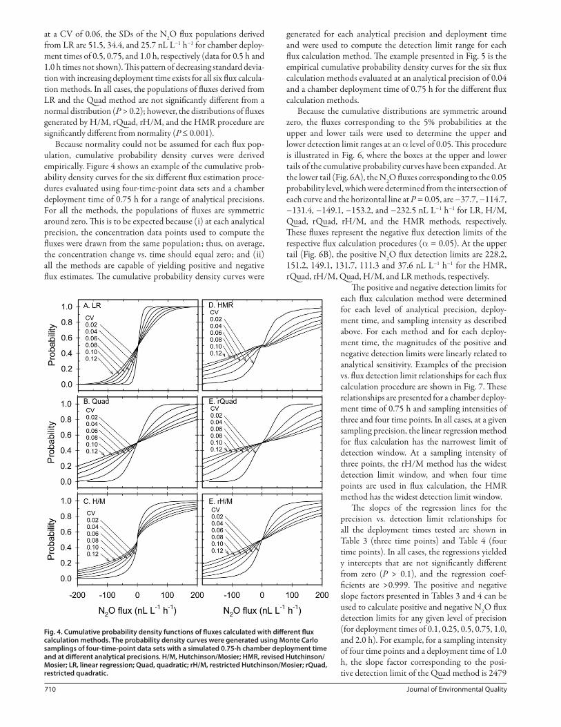
Because normality could not be assumed for each fl ux pop-ulation, cumulative probability density curves were derived empirically. Figure 4 shows an example of the cumulative prob-ability density curves for the six diff erent fl ux estimation proce-dures evaluated using four-time-point data sets and a chamber deployment time of 0.75 h for a range of analytical precisions. For all the methods, the populations of fl uxes are symmetric around zero. Th is is to be expected because (i) at each analytical precision, the concentration data points used to compute the fl uxes were drawn from the same population; thus, on average, the concentration change vs. time should equal zero; and (ii) all the methods are capable of yielding positive and negative fl ux estimates. Th e cumulative probability density curves were

generated for each analytical precision and deployment time and were used to compute the detection limit range for each fl ux calculation method. Th e example presented in Fig. 5 is the empirical cumulative probability density curves for the six fl ux calculation methods evaluated at an analytical precision of 0.04 and a chamber deployment time of 0.75 h for the diff erent fl ux calculation methods.

Because the cumulative distributions are symmetric around zero, the fl uxes corresponding to the 5% probabilities at the upper and lower tails were used to determine the upper and lower detection limit ranges at an α level of 0.05. Th is procedure is illustrated in Fig. 6, where the boxes at the upper and lower tails of the cumulative probability curves have been expanded. At the lower tail (Fig. 6A), the N2O fl uxes corresponding to the 0.05 probability level, which were determined from the intersection of each curve and the horizontal line at P = 0.05, are −37.7, −114.7, −131.4, −149.1, −153.2, and −232.5 nL L−1 h−1 for LR, H/M, Quad, rQuad, rH/M, and the HMR methods, respectively. Th ese fl uxes represent the negative fl ux detection limits of the respective fl ux calculation procedures (α = 0.05). At the upper tail (Fig. 6B), the positive N2O fl ux detection limits are 228.2, 151.2, 149.1, 131.7, 111.3 and 37.6 nL L−1 h−1 for the HMR, rQuad, rH/M, Quad, H/M, and LR methods, respectively.

Th e positive and negative detection limits for each fl ux calculation method were determined for each level of analytical precision, deploy-ment time, and sampling intensity as described above. For each method and for each deploy-ment time, the magnitudes of the positive and negative detection limits were linearly related to analytical sensitivity. Examples of the precision vs. fl ux detection limit relationships for each fl ux calculation procedure are shown in Fig. 7. Th ese relationships are presented for a chamber deploy-ment time of 0.75 h and sampling intensities of three and four time points. In all cases, at a given sampling precision, the linear regression method for fl ux calculation has the narrowest limit of detection window. At a sampling intensity of three points, the rH/M method has the widest detection limit window, and when four time points are used in fl ux calculation, the HMR method has the widest detection limit window.

Th e slopes of the regression lines for the precision vs. detection limit relationships for all the deployment times tested are shown in Table 3 (three time points) and Table 4 (four time points). In all cases, the regressions yielded y intercepts that are not signifi cantly diff erent from zero (P > 0.1), and the regression coef-fi cients are >0.999. Th e positive and negative slope factors presented in Tables 3 and 4 can be used to calculate positive and negative N2O fl ux detection limits for any given level of precision (for deployment times of 0.1, 0.25, 0.5, 0.75, 1.0, and 2.0 h). For example, for a sampling intensity of four time points and a deployment time of 1.0 h, the slope factor corresponding to the posi-tive detection limit of the Quad method is 2479

Fig. 4. Cumulative probability density functions of fl uxes calculated with diff erent fl ux calculation methods. The probability density curves were generated using Monte Carlo samplings of four-time-point data sets with a simulated 0.75-h chamber deployment time and at diff erent analytical precisions. H/M, Hutchinson/Mosier; HMR, revised Hutchinson/Mosier; LR, linear regression; Quad, quadratic; rH/M, restricted Hutchinson/Mosier; rQuad, restricted quadratic.


(Table 4). If the sampling precision (CV) for N2O is 0.065, the positive detection limit of the Quad method would be 2479 × 0.065 = 161.1 nL L−1 h−1.

Scaled ResultsTh e conversion factors for computing fl ux detection limits

shown in Tables 3 and 4 are only valid for N2O at ambient levels of 320 nL L−1. However, these results were scaled, so they are applicable to any gas at any ambient concentration. Scaling was done by dividing the slope factors by the 320 (the ambi-ent N2O concentration used in the Monte Carlo simulations). Tables 5 and 6 show the scaled slope factors associated with each fl ux calculation method over the range of deployment times tested. Th e scaled slope factors can be used to compute fl ux detection limits for any gas if the ambient concentration of the gas of interest is known. For example, consider the sce-nario where three time points are collected over a chamber deployment time of 0.75 h and an ambient CH4 concentration of 1.75 μL L−1. From Table 5, it is determined that the scaled slope factors defi ning the precision vs. fl ux detection limits relationships for LR are −3.10 (negative fl ux detection limit) and 3.100 (positive fl ux detection limit). Conversion of these scaled slopes to factors to CH4 is done by multiplying by the ambient CH4 concentration. Th us, the negative and positive slope factors for CH4 fl ux detection at a chamber deployment time of 0.75 h are −5.425 and 5.425, respectively. If the analyti-cal precision for CH4 detection at ambient levels is 0.096, then the positive and negative detection limits for CH4 fl uxes calcu-lated using LR would be −5.425 × 0.096 = −0.521 μL L−1 CH4 h−1 and 5.425 × 0.096 = 0.521 μL L−1 CH4 h−1, respectively. Th e scaled slope factors shown in Tables 5 and 6 are only valid for the chamber deployment times listed.

Fig. 5. Cumulative probability density functions of fl uxes calculated with the six methods for an analytical precision of 0.04, chamber deployment time of 0.75 h, and sampling intensity of four points. Expanded views of the upper and lower tails of the distribution (boxes) are shown in Fig. 6. H/M, Hutchinson/Mosier; HMR, revised Hutchinson/Mosier; LR, linear regression; Quad, quadratic; rH/M, restricted Hutchinson/Mosier; rQuad, restricted quadratic.

Fig. 6. Expanded views of the lower (A) and upper (B) tails of the cumulative probability distributions functions shown in Fig. 5. The dotted lines in the fi gures show how the fl uxes of each method cor-responding to the 0.05 (Fig. 6A) and 0.95 (Fig. 6B) probability levels were determined. H/M, Hutchinson/Mosier; HMR, revised Hutchinson/Mosier; LR, linear regression; Quad, quadratic; rH/M, restricted Hutchinson/Mosier; rQuad, restricted quadratic.

Fig. 7. Relationships between analytical precision and the positive and negative fl ux detection limits of the diff erent fl ux calculation methods when three-time-point (A) or four-time-point (B) data series are used. H/M, Hutchinson/Mosier; HMR, revised Hutchinson/Mosier; LR, linear regression; Quad, quadratic; rH/M, restricted Hutchinson/Mosier; rQuad, restricted quadratic.


Table 3. Factors (slopes) relating precision to N2O fl ux detection limit for diff erent fl ux calculation methods using three time points at diff erent

deployment times. Factors are slopes of the regression lines shown in Fig. 7. The y-intercepts of the regressions were not signifi cantly diff erent from zero.†

Deployment time

Negative limit of detection slope Positive limit of detection slope

LR‡ Quad H/M rQuad rH/M LR Quad H/M rQuad rH/M

h ———————————————————————————— nL L−1 h−1 CV−1 ————————————————————————————

0.1 −7,506 −26,851 −22,659 −29,878 −31,758 7,465 26,863 22,163 29,914 31,167

0.25 −2,977 −10,698 −8,942 −11,913 −12,742 2,966 10,694 9,066 11,885 12,834

0.5 −1,490 −5,375 −4,518 −5,963 −6,349 1,488 5,383 4,540 5,967 6,346

0.75 −992 −3,594 −3,031 −3,995 −4,268 993 3,578 3,037 3,972 4,276

1.0 744 −2,679 −2,275 −2,966 −3,187 743 2,689 2,240 2,988 3,158

2.0 −371 −1,338 −1,139 −1,484 −1,603 374 1,349 1,140 1,506 1,601

† In all cases, r2 values exceeded 0.9996.

‡ H/M, Hutchinson/Mosier; HMR, revised Hutchinson/Mosier; LR, linear regression; Quad, quadratic; rH/M, restricted Hutchinson/Mosier; rQuad,


Table 4. Factors relating precision to detection limit of fl uxes determined with four fl ux calculation methods using four time points for diff erent deployment times. Factors are slopes of the regression lines shown in Fig. 7. The y-intercepts of the regressions were not signifi cantly diff erent from zero.†

Deployment time

Negative limit of detection slope Positive limit of detection slope

LR‡ Quad H/M rQuad rH/M HMR LR Quad H/M rQuad rH/M HMR

h ————————————————————————————— nL L−1 h−1 CV−1 —————————————————————————————

0.1 −7,033 −24,620 −21,165 −28,153 −28,493 −41,370 7,036 24,570 20,725 28,002 28,112 42,547

0.25 −2,819 −9,846 −2,529 −11,261 −11,711 −16,746 2,824 9,862 8,543 11,278 11,650 17,091

0.5 −1,414 −4,935 −4,312 −5,653 −5,831 −8,380 1,411 4,943 4,290 5,649 5,768 8,400

0.75 −944 −3,289 −2,863 −3,757 −3,816 −5,573 939 3,305 2,858 3,776 3,875 5,835

1.0 −708 −2,471 −2,114 −2,829 −2,883 −4,120 707 2,479 2,143 2,835 2,881 4,216

2.0 −353 −1,238 −1,069 −1,410 −1,429 −1,990 352 1,230 1,066 1,400 1,447 2,163

† In all cases, r2 values exceeded 0.9996.

‡ H/M, Hutchinson/Mosier; HMR, revised Hutchinson/Mosier; LR, linear regression; Quad, quadratic; rH/M, restricted Hutchinson/Mosier; rQuad,


Table 5. Scaled slope factors relating precision to detection limit of fl uxes determined with calculation procedures using three time points for diff er-ent deployment times. Scaled slopes were calculated by dividing the corresponding slopes in Table 3 by the ambient mean N

2O concentration (320

ppb) used in the Monte Carlo simulations.

Deployment time

Negative limit of detection factor Positive limit of detection factor

LR† Quad H/M rQuad rH/M LR Quad H/M rQuad rH/M

h ————————————————————————————— h−1 CV−1 —————————————————————————————

0.1 −23.5 −83.9 −70.8 −93.4 −99.2 23.3 83.9 69.3 93.5 97.4

0.25 −9.30 −33.4 −27.9 −37.2 −39.8 9.27 33.4 28.3 37.0 40.1

0.5 −4.66 −16.8 −14.1 −18.6 −19.8 4.65 16.8 14.2 18.6 19.8

0.75 −3.10 −11.2 −9.47 −12.5 −13.3 3.10 11.2 9.49 12.4 13.4

1.0 −2.33 −8.37 −7.11 −9.27 −9.96 2.32 8.40 7.00 9.34 9.87

2.0 −1.16 −4.18 −3.56 −4.64 −5.01 1.17 4.22 3.56 4.71 5.00

† H/M, Hutchinson/Mosier; HMR, revised Hutchinson/Mosier; LR, linear regression; Quad, quadratic; rH/M, restricted Hutchinson/Mosier; rQuad,


Table 6. Scaled slope factors relating precision to detection limit of fl uxes determined with calculation procedures using four time points for diff er-ent deployment times. Scaled slopes were calculated by dividing the corresponding slopes in Table 4 by the ambient mean N

2O concentration (320

ppb) used in the Monte Carlo simulations.

Deployment time

Negative limit of detection scaled factor Positive limit of detection scaled factor

LR† Quad H/M rQuad rH/M HMR LR Quad H/M rQuad rH/M HMR

h —————————————————————————————— h−1 CV−1 ——————————————————————————————

0.1 −22.0 −76.9 −66.1 −88.0 −89.0 −129.3 22.0 76.8 64.8 87.5 87.9 133.0

0.25 −8.81 −30.8 −7.90 −35.2 −36.6 −52.33 8.83 30.8 26.7 35.2 36.4 53.4

0.5 −4.42 −15.4 −13.5 −17.7 −18.2 −26.2 4.41 15.4 13.4 17.7 18.0 26.3

0.75 −2.95 −10.3 −8.95 −11.4 −11.9 −17.0 2.93 10.3 8.93 11.8 12.1 18.1

1.0 −2.21 −7.72 −6.6 −8.84 −9.00 −12.9 2.21 7.75 6.70 8.86 9.00 13.2

2.0 −1.10 −3.87 −3.34 −4.41 −4.47 −6.22 1.10 3.84 3.33 4.38 4.52 6.76

† H/M, Hutchinson/Mosier; HMR, revised Hutchinson/Mosier; LR, linear regression; Quad, quadratic; rH/M, restricted Hutchinson/Mosier; rQuad,



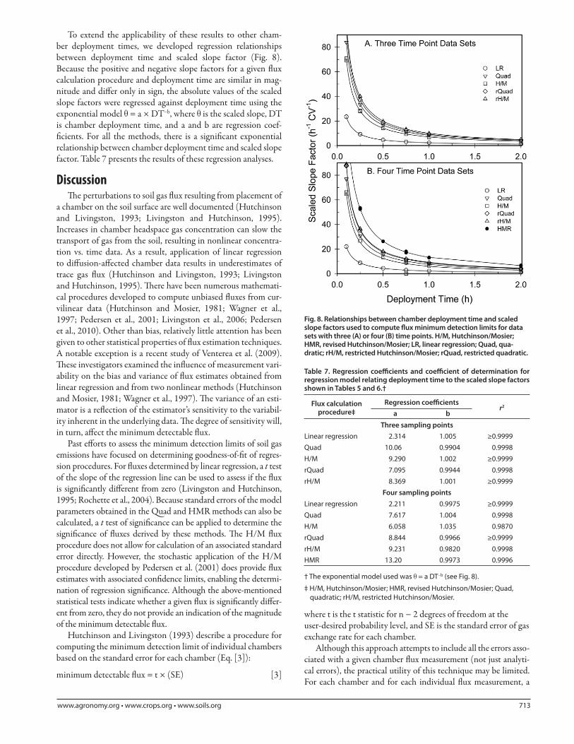
To extend the applicability of these results to other cham-ber deployment times, we developed regression relationships between deployment time and scaled slope factor (Fig. 8). Because the positive and negative slope factors for a given fl ux calculation procedure and deployment time are similar in mag-nitude and diff er only in sign, the absolute values of the scaled slope factors were regressed against deployment time using the exponential model θ = a × DT−b, where θ is the scaled slope, DT is chamber deployment time, and a and b are regression coef-fi cients. For all the methods, there is a signifi cant exponential relationship between chamber deployment time and scaled slope factor. Table 7 presents the results of these regression analyses.

DiscussionTh e perturbations to soil gas fl ux resulting from placement of

a chamber on the soil surface are well documented (Hutchinson and Livingston, 1993; Livingston and Hutchinson, 1995). Increases in chamber headspace gas concentration can slow the transport of gas from the soil, resulting in nonlinear concentra-tion vs. time data. As a result, application of linear regression to diff usion-aff ected chamber data results in underestimates of trace gas fl ux (Hutchinson and Livingston, 1993; Livingston and Hutchinson, 1995). Th ere have been numerous mathemati-cal procedures developed to compute unbiased fl uxes from cur-vilinear data (Hutchinson and Mosier, 1981; Wagner et al., 1997; Pedersen et al., 2001; Livingston et al., 2006; Pedersen et al., 2010). Other than bias, relatively little attention has been given to other statistical properties of fl ux estimation techniques. A notable exception is a recent study of Venterea et al. (2009). Th ese investigators examined the infl uence of measurement vari-ability on the bias and variance of fl ux estimates obtained from linear regression and from two nonlinear methods (Hutchinson and Mosier, 1981; Wagner et al., 1997). Th e variance of an esti-mator is a refl ection of the estimator’s sensitivity to the variabil-ity inherent in the underlying data. Th e degree of sensitivity will, in turn, aff ect the minimum detectable fl ux.

Past eff orts to assess the minimum detection limits of soil gas emissions have focused on determining goodness-of-fi t of regres-sion procedures. For fl uxes determined by linear regression, a t test of the slope of the regression line can be used to assess if the fl ux is signifi cantly diff erent from zero (Livingston and Hutchinson, 1995; Rochette et al., 2004). Because standard errors of the model parameters obtained in the Quad and HMR methods can also be calculated, a t test of signifi cance can be applied to determine the signifi cance of fl uxes derived by these methods. Th e H/M fl ux procedure does not allow for calculation of an associated standard error directly. However, the stochastic application of the H/M procedure developed by Pedersen et al. (2001) does provide fl ux estimates with associated confi dence limits, enabling the determi-nation of regression signifi cance. Although the above-mentioned statistical tests indicate whether a given fl ux is signifi cantly diff er-ent from zero, they do not provide an indication of the magnitude of the minimum detectable fl ux.

Hutchinson and Livingston (1993) describe a procedure for computing the minimum detection limit of individual chambers based on the standard error for each chamber (Eq. [3]):

minimum detectable fl ux = t × (SE) [3]

where t is the t statistic for n − 2 degrees of freedom at the user-desired probability level, and SE is the standard error of gas exchange rate for each chamber.

Although this approach attempts to include all the errors asso-ciated with a given chamber fl ux measurement (not just analyti-cal errors), the practical utility of this technique may be limited. For each chamber and for each individual fl ux measurement, a

Fig. 8. Relationships between chamber deployment time and scaled slope factors used to compute fl ux minimum detection limits for data sets with three (A) or four (B) time points. H/M, Hutchinson/Mosier; HMR, revised Hutchinson/Mosier; LR, linear regression; Quad, qua-dratic; rH/M, restricted Hutchinson/Mosier; rQuad, restricted quadratic.

Table 7. Regression coeffi cients and coeffi cient of determination for regression model relating deployment time to the scaled slope factors shown in Tables 5 and 6.†

Flux calculation procedure‡

Regression coeffi cientsr2

a b

Three sampling points

Linear regression 2.314 1.005 ≥0.9999

Quad 10.06 0.9904 0.9998

H/M 9.290 1.002 ≥0.9999

rQuad 7.095 0.9944 0.9998

rH/M 8.369 1.001 ≥0.9999

Four sampling points

Linear regression 2.211 0.9975 ≥0.9999

Quad 7.617 1.004 0.9998

H/M 6.058 1.035 0.9870

rQuad 8.844 0.9966 ≥0.9999

rH/M 9.231 0.9820 0.9998

HMR 13.20 0.9973 0.9996

† The exponential model used was θ = a DT−b (see Fig. 8) .

‡ H/M, Hutchinson/Mosier; HMR, revised Hutchinson/Mosier; Quad,

quadratic; rH/M, restricted Hutchinson/Mosier.


diff erent SE is derived. Th us, the minimum detectable fl ux will be diff erent for each chamber each time a fl ux is measured. We applied this technique in our Monte Carlo study, and, for linear regression with three time points, we observed that Eq. [3] yielded minimum detectable fl ux values that ranged from 1945 nL L−1 h−1 to 0.0048 nL L−1 h−1 for an analytical precision of 0.05 and a chamber deployment time of 0.75 h.

Verchot et al. (1999) recognized the limitations associated with the minimum fl ux detection calculation identifi ed in Eq. [3] and implemented a modifi cation of the regression signifi -cance procedure whereby all their measured fl uxes were ranked. Th e minimum detection limit was then determined as the fl ux threshold where >67% of the measured fl uxes were signifi cant. Th ese authors reported a minimum detectable fl ux for N2O emission of 0.6 ng N cm−2 h−1. To compare this value with our results, we used the Verchot et al. (1999) chamber dimensions, deployment time, and sampling intensity to calculate that a fl ux of 0.6 ng N cm−2 h−1 corresponds to a headspace concentration change of detection limit of 29.9 nL L−1 h−1 (at 25°C and 1 atmo-sphere pressure). Results of our study indicate that this detection limit corresponds to a measurement precision of approximately 0.02 (at four sampling points, a 0.5-h deployment, and an ambi-ent N2O concentration of 320 nL L−1). Th e approach adopted by Verchot et al. (1999) is more defensible than simply assessing regression goodness of fi t; however, the assumption that 67% of the signifi cant fl uxes in any given data set exceed the actual mini-mum detectable fl ux is arbitrary.

Assessment of the minimum detectable fl ux could be deter-mined experimentally by placing a chamber on a non–trace gas producing surface (e.g., a linoleum fl oor), sampling the head-space gas concentration of the chamber over time, and com-puting an apparent fl ux. However, this process would have to be repeated extensively to obtain reliable probability estimates associated with each fl ux determination. Monte Carlo sampling allows for the same analysis to be conducted mathematically and facilitates assessment of the eff ects of measurement precision on detection limit. In our evaluations we minimized the Type II error rate associated with the regression analyses by imposing the condition that all the regression-derived fl uxes (LR, Quad, rQuad, and HMR) are signifi cantly diff erent from zero. Th us, the fl ux detection limits calculated by our procedure can be con-sidered conservative estimates.

We observed linear relationships between analytical precision and minimum detectable fl ux. In addition to analytical and sam-pling precision, chamber deployment time, sampling intensity, and fl ux calculation method aff ect the detection limits associ-ated with chamber headspace gas concentration changes over

time. Th e regression relationships shown in Table 7 summarize these eff ects and can be used to compute a minimum detection limit for any gas.

As an illustration, we used the mean ambient concentrations and the associated sampling and analytical precision estimates shown in Fig. 2 to calculate the minimum detectable fl uxes for N2O, CH4, and CO2 determined by the Quad method (Table 8). Th e fi rst step in implementing this procedure is to calculate θ (the scaled slope factor using the coeffi cients of the exponen-tial equation associated with the rQuad method with three time points). Th e slope factor for each gas is then calculated by multiplying θ by the ambient concentration of the gas of inter-est. Th e resulting slope factors for each gas are multiplied by the sampling and analytical precision of each gas to obtain the positive fl ux detection limit. Multiplication of the positive fl ux detection limits by −1 yields the negative fl ux detection limits. Th ese fl ux detection limits have units of ηL−1 h−1. Conversion of these values to fl ux units of mass per unit area can easily be done if the temperature, pressure, and chamber dimensions are known. When this is done, chamber size (specifi cally height) aff ects how the ηL L−1 h−1 detection limit is translated into a gas fl ux value expressed on an areal basis. A detailed description of fl ux detection limit calculations is provided in the supplemen-tary materials.

Despite the method used to compute the minimum detection limit (MDL), consideration must be given to how fl uxes that fall below the limit are treated. Th ere are several options available to handle data that fall below the MDL (or within the detection limit band). Th ese options are summarized by Gilbert (1987) and include (i) report the value as “below the detection limit,” (ii) report the value as zero, (iii) report some values between zero and the MDL (such as one half the MDL), or (iv) report the actual measured value even if it falls below the MDL. Of these options, Gilbert (1987) recommends the latter as the least biased course of action (i.e., report the measured value along with the stated MDL).

Due to variability in concentration vs. time data, no single fl ux calculation scheme will be applicable (or optimal) over the entire range of concentration vs. time data series encountered. For example, in cases where (C1 − C0)/(C2 − C1) < 0, the Quad, H/M, or HMR methods may not be applicable. In these cases, LR could be used. Th erefore, rather than recommending a single fl ux calculation method to the exclusion of others, we suggest that “hybrid” fl ux calculation schemes be adopted whereby a linear regression is used when a given data set does not conform to a nonlinear model. Such a hybrid scheme is resident in the HMR soft ware, which provides a linear fl ux when the HMR model fails. Th e coeffi cients provided in Table 7 can be used in

Table 8. Examples of how the equation for the rQuad fl ux calculation method is used to calculate fl ux detection limits for N2O, CH

4, and CO

2 when

the ambient concentrations and analytical precisions are known (shown in Fig. 3) with three time points of data and a deployment time of 0.667 h. Exponential model regression coeffi cients (shown in Table 7) that relate chamber deployment time to the rQuad slope factor were used.

Parameter N2O CH

4CO

2

Mean ambient concentration, ηL−1 (N2O); mL L−1 (CH

4 and CO

2) 323 1.79 385.5

Precision, CV 0.044 0.071 0.0014

Deployment time, h 0.667 0.667 0.667

θ (calculated from Table 7, rQuad method, three time points, 0.667 h deployment time) 10.61 10.61 10.61

Slope factor (θ × mean concentration) 3428 18.99 4091

Positive fl ux detection limit, ppb h−1 or ppm h−1 (slope factor × CV) 150.8 1.349 5.728

Negative fl ux detection limit, ppb h−1 or ppm h−1 (−1 × slope factor × CV) −150.8 −1.349 −5.728


the manner illustrated in Table 8 to compute the MDL for each of the individual fl ux calculation methods used within such a hybrid scheme.

Our study only considered sampling and analytical precision associated with trace gas concentration measurement. Other sources of variability (e.g., chamber leakage, changes in biological activity during the chamber deployment period) may also reduce measurement precision. However, our assessment of analyti-cal precision mirrors the methodology used to collect chamber gas samples in the fi eld. Our results on the minimum detectable fl uxes associated with each fl ux calculation method should not be the only consideration in selecting a fl ux calculation method. For any given level of precision and deployment time, linear regression had the narrowest detection window, yet this method is known to yield biased estimates in some situations. However, methods that attempt to correct for diff usion eff ects on chamber headspace gas concentration data (i.e., Quad, H/M, HMR) may not be appropriate in all data sets. We are currently expanding our investigations of the bias and variance associated with diff er-ent fl ux calculation methods to identify specifi c criteria that will enable recommendation of one technique over another. Finally, because of the increasing importance being placed on estimates of soil GHG emissions, we recommend that reports of soil trace gas fl ux include information about sampling and analytical preci-sion and associated estimates of minimum detectable fl uxes.

ReferencesAmerican Public Health Association. 1985. Precision, accuracy and correctness

of analyses. In: A.E. Greenberg, R.R. Trussell, and L.S. Clesceri, editors, Standard methods for the analysis of water and wastewater. American Pub-lic Health Association, Washington, DC. p. 20–36.

Anthony, W.H., G.L. Hutchinson, and G.P. Livingston. 1995. Chamber measurement of soil-atmosphere gas exchange: Linear vs. diff usion-based fl ux models. Soil Sci. Soc. Am. J. 59:1308–1310. doi:10.2136/sssaj1995.03615995005900050015x

Arnold, S., T.B. Parkin, J.W. Doran, and A.R. Mosier. 2001. Automated gas sam-pling system for laboratory analysis of CH4 and N2O. Commun. Soil Sci. Plant Anal. 32:2795–2807. doi:10.1081/CSS-120000962

Box, G.E.P., and M.E. Muller. 1958. A note on the generation of random normal deviates. Ann. Math. Stat. 29:610–611. doi:10.1214/aoms/1177706645

Emerson, J.D., and M.A. Stoto. 1983. Transforming data. In: D.C. Hoaglin, F. Mosteller, and J.W. Tukey, editors, Understanding robust and exploratory data analysis. John Wiley & Sons, New York. p. 97–120.

Gilbert, R.O. 1987. Statistical methods for environmental pollution monitoring. Van Nostrand Reinhold Co., New York.

Healy, R.W., R.G. Striegl, T.F. Rusell, G.L. Hutchinson, and G.P. Livingston. 1996. Numerical evaluation of static- chamber measurements of soil-atmo-sphere gas exchange: Identifi cation of physical processes. Soil Sci. Soc. Am. J. 60:740–747. doi:10.2136/sssaj1996.03615995006000030009x

Hutchinson, G.L., and G.P. Livingston. 1993. Use of chamber systems to mea-sure trace gas fl uxes. In: L. Harper et al., editors, Agricultural ecosystem eff ects on trace gases and global climate change. ASA Spec. Publ. 55. ASA, CSSA, SSSA, Madison, WI. p. 63–78.

Hutchinson, G.L., and A.R. Mosier. 1981. Improved soil cover method for fi eld measurement of nitrous oxide fl uxes. Soil Sci. Soc. Am. J. 45:311–316. doi:10.2136/sssaj1981.03615995004500020017x

Livingston, G.P., and G.L. Hutchinson. 1995. Enclosure-based measurement of trace gas exchange: Applications and sources of error. In: P.A. Matson and R.C. Harriss, editors, Biogenic trace gases: Measuring emissions from soil and water. Methods in Ecology. Blackwell Science/Cambridge Univ. Press, Cambridge, UK. p. 14–51.

Livingston, G.P., G.L. Hutchinson, and K. Spartalian. 2006. Trace gas emission in chambers: A non-steady-state diff usion model. Soil Sci. Soc. Am. J. 70:1459–1469. doi:10.2136/sssaj2005.0322

Pedersen, A.R., S.O. Petersen, and F.P. Vinther. 2001. Stochastic diff usion model for estimating trace gas emissions with static chambers. Soil Sci. Soc. Am. J. 65:49–58. doi:10.2136/sssaj2001.65149x

Pedersen, A.R., S.O. Petersen, and K. Schelde. 2010. A comprehensive approach to soil-atmosphere trace-gas fl ux estimation with static chambers. Eur. J. Soil Sci. 61:888–902. doi:10.1111/j.1365-2389.2010.01291.x

Rochette, P., D.A. Angers, M.H. Chantigny, N. Bertrand, and D. Cote. 2004. Carbon dioxide and nitrous oxide emissions following fall and spring ap-plications of pig slurry to an agricultural soil. Soil Sci. Soc. Am. J. 68:1410–1420. doi:10.2136/sssaj2004.1410

Rochette, P., and N. Bertrand. 2007. Soil-surface gas emissions. In: M. Carter and E.G. Gregorich, editors, Soil sampling and methods of analysis. 2nd ed. CRC Press, Boca Raton, FL. p. 851–861.

Rochette, P., and N.S. Eriksen-Hamel. 2008. Chamber measurements of soil ni-trous oxide fl ux: Are absolute values reliable? Soil Sci. Soc. Am. J. 72:331–342. doi:10.2136/sssaj2007.0215

Venterea, R.T. 2010. Simplifi ed method for quantifying theoretical underesti-mation of chamber-based trace gas fl uxes. J. Environ. Qual. 39:126–135. doi:10.2134/jeq2009.0231

Venterea, R.T., and J.M. Baker. 2008. Eff ects of soil physical nonuniformity on chamber-based gas fl ux estimates. Soil Sci. Soc. Am. J. 72:1410–1417. doi:10.2136/sssaj2008.0019

Venterea, R.T., K.A. Spokas, and J.M. Baker. 2009. Accuracy and precision analy-sis of chamber-based nitrous oxide gas fl ux estimates. Soil Sci. Soc. Am. J. 73:1087–1093. doi:10.2136/sssaj2008.0307

Verchot, L.V., E.A. Davidson, J.H. Cattânio, I.L. Ackerman, H.E. Erickson, and M. Keller. 1999. Land use change and biogeochemical controls of nitrogen oxide emissions from soils in eastern Amozonia. Global Biogeochemical Cycles. 13:31–46.

Wagner, S.W., D.C. Reicosky, and R.S. Alessi. 1997. Regression models for cal-culating gas fl uxes measured with a closed chamber. Agron. J. 89:279–284. doi:10.2134/agronj1997.00021962008900020021x

calculating the detection limits of chamber-based soil ... parkin et al... · calculating the...

Documents