Frequenc y Offset Trackingin MCMA Systems

ChristianStimmingstimming@tuhh.de

May 29,2001

Contents

1 Introduction 2

2 Frequenc y Offset 22.1 OffsetDerivation . . . . . . . . . . . . . . . . . . . . . . . . . . . . . . . . . . . . . 22.2 ChannelModel . . . . . . . . . . . . . . . . . . . . . . . . . . . . . . . . . . . . . . 32.3 Receiver Model . . . . . . . . . . . . . . . . . . . . . . . . . . . . . . . . . . . . . . 5

3 Digital Phase Locked Loop 53.1 PLL Structure . . . . . . . . . . . . . . . . . . . . . . . . . . . . . . . . . . . . . . . 53.2 LoopFilter Order . . . . . . . . . . . . . . . . . . . . . . . . . . . . . . . . . . . . . 63.3 LoopFilter Structure . . . . . . . . . . . . . . . . . . . . . . . . . . . . . . . . . . . 73.4 LoopFilter Coefficients . . . . . . . . . . . . . . . . . . . . . . . . . . . . . . . . . . 83.5 Stability . . . . . . . . . . . . . . . . . . . . . . . . . . . . . . . . . . . . . . . . . . 83.6 NaturalFrequency . . . . . . . . . . . . . . . . . . . . . . . . . . . . . . . . . . . . 103.7 DampingFactor . . . . . . . . . . . . . . . . . . . . . . . . . . . . . . . . . . . . . . 113.8 NoiseNumber. . . . . . . . . . . . . . . . . . . . . . . . . . . . . . . . . . . . . . . 123.9 PhaseError Detection. . . . . . . . . . . . . . . . . . . . . . . . . . . . . . . . . . . 14

4 Application 154.1 Single-carrierSVD . . . . . . . . . . . . . . . . . . . . . . . . . . . . . . . . . . . . 154.2 Single-carrierMMSE-QRD . . . . . . . . . . . . . . . . . . . . . . . . . . . . . . . . 164.3 Single-antennaOFDM . . . . . . . . . . . . . . . . . . . . . . . . . . . . . . . . . . 174.4 SimulinkBlock Library . . . . . . . . . . . . . . . . . . . . . . . . . . . . . . . . . . 21

5 Fix-Point Implementa tion 245.1 ScalingFactor . . . . . . . . . . . . . . . . . . . . . . . . . . . . . . . . . . . . . . . 245.2 DiscreteCoefficients . . . . . . . . . . . . . . . . . . . . . . . . . . . . . . . . . . . 24

1

6 Conc lusions 25

7 Acknowledgm ents 26

1 Intr oduction

Motivatedby the significantcapacitygain of multiple-antenna systems,several multi-antennatrans-ceiver systemsareunderinvestigationat theBerkeley WirelessResearchCenter1. In [1], a theoreticalframework for a multi-carriermulti-antennasystemwasdeveloped.However, anactualimplementa-tion remainsyet to becompleted.

Simulationresultsin SIMULINK indicatethataMCMA systemhasvery stringentrequirementsonthefrequency synchronizationbetweentransmitterandreceiver. This reportdevelopsbuilding blocksin SIMULINK for thefrequency offsetcorrectionandtrackingto beusedin a MCMA system.

This projectwork wasdoneat the Berkeley WirelessResearchCenterin February2001throughMay 2001. Theauthorwasvisiting Berkeley in a specialexchangeprogramwith theTechnicalUni-versity of Hamburg-Harburg. This projectwork servesasa pre-thesisprojectwork (“Studienarbeit”)for theGermanMS degree(“Diplom”).

������� ��� ��� � ����� � ����� � ����� ������� ��� �������Channel

Figure1: SimpleFrequency OffsetModel

2 Frequenc y Offset

2.1 Offset Deriv ation

The senderand receiver of a transmissionsystemus an oscillator for up-mixing and down-mixingof the signal to the bandpassregion andback. Thoseoscillatorsarenot the same,andtherewill besomefrequency offsetbetweenthem.Theoffset leadsto a rotationof theconstellationdiagramat thereceiver which is proportionalto thefrequency differencebetweenthetwo oscillators.This is derivedasfollows.

Let ������� bethediscretesymbolsto betransmitted,and � ����� the impulseshapefor eachsymbol.Thecontinuoustransmittedbase-bandsignalis (figure1)����!"�$#&%(')�������*� ��� +-,.!"� (1)

1http://bwrc.eecs.berkeley.edu

2

Transmitter

Channel

Receiver����/0� 1 ��/0� 23��/0�4���5�6�7�8 ����/0�

Figure2: Channelmodelwith Frequency Offset(Signalsat symbolrate)

Thesignalis runthroughamixer thatmodulates����!"� to thecarrierfrequency, usingacrystaloscillatorat frequency 9�: , whichgives ; ��!"��#&<�=�>(?"@ A ����!"� (2)

asthe transmittedsignal. Undertheassumptionof a perfectchannelBC��!"� , thereceived signal D0��!"�E#; ��!"�GFHBC��!"� is identicalto the transmittedsignal, D0��!"�H# ; ��!"� . Thereceiver will down-mix thesignalusing a different crystal oscillator with a different frequency I9�: , resultingin the received low-passsignal J ��!"�G#&<(K =(L>(M@ A D0��!"��#&< =�NO>(M K L>(M"PQ@ A(����!"� (3)

We definethedifferencebetweenbothmixer frequenciesas RS9&#T9�:E,UI9�:V#)W XYA(R[Z \ , andwecall R[Z \ thefrequency offset.Thismeansthateachreceivedsymbolhasa phaseoffsetaccordingtoJ ��� +]��#&< =^�> '�_ ����� +]� (4)

i.e. theconstellationdiagramis rotatingwith anangleof RS9G+ per symbolperiod + . We definethephaseerrorat symbol � as ` �����$#&RS9aA�� + (5)

The PLL of the analogfront-endadditionallyhassomephasenoisethat will result in a phasejitter` = ����� thataddsto thephaseerror.` = ����� is a randomprocesswith somepower spectrumdetermined

by thetypeof PLL. Thetotal phaseerrorthenis definedas` �����$#&RS9aA�� +cb ` = ����� (6)

2.2 Channel Model

Thephaseerror(5) is includedin thechannelmodelasshown in figure2. For now, weignoretheeffectof thephasejitter/phasenoise.ThereceivedsymbolsaregivenbyJ �����G#&< =d3N ' P A(e������ Ff������� bcg������ (7)

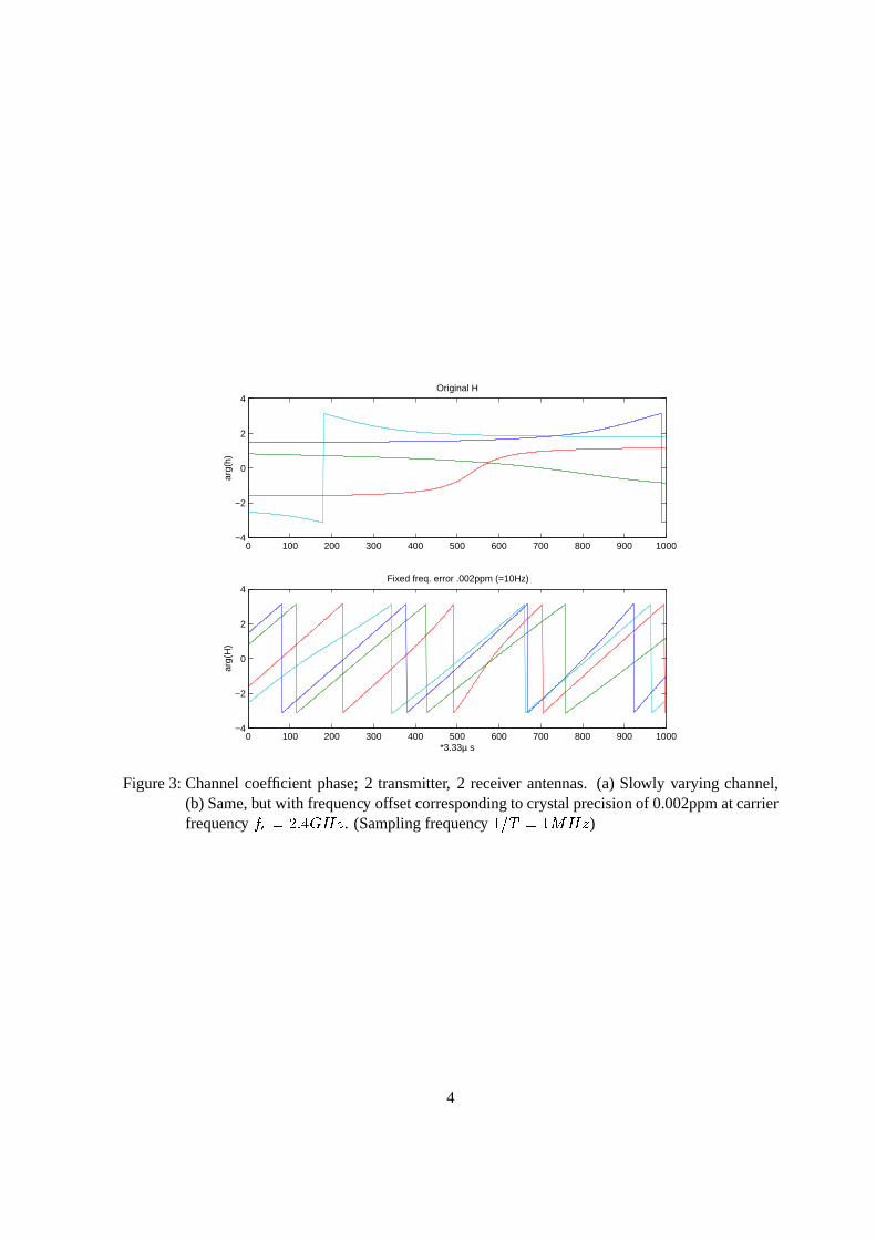
where e������ is thechannelimpulseresponseand g������ is additive noise.If thetransmissionmodelsofar assumeda slowly varyingchannel,thentheadditionalphaseterm< =d3N ' P eliminatesthisproperty. Figure3 showsthephaseof channelcoefficientsof atwo-by-two multi-

antennatransmissionsystem.Theoriginalmodel(figure3(a))is slowly varying.But with averysmallfrequency offset(figure3(b)) theassumptionof slow variancedoesno longerhold. It is thereforevitalthatany receiver structuredealswith this phaseerrorandcorrectsit.

3

0 100 200 300 400 500 600 700 800 900 1000−4

−2

0

2

4Original H

arg(

h)

0 100 200 300 400 500 600 700 800 900 1000−4

−2

0

2

4Fixed freq. error .002ppm (=10Hz)

arg(

H)

*3.33µ s

Figure3: Channelcoefficient phase;2 transmitter, 2 receiver antennas.(a) Slowly varying channel,(b) Same,but with frequency offsetcorrespondingto crystalprecisionof 0.002ppmatcarrierfrequency Z \h#iW�jlkCm]nog . (Samplingfrequency p(q +&#Tp rTnog )

4

Transmitter

Channel����/0� 1 ��/0� 23��/0�4���5�6�7�8 ����/0� Receiver

������5�6�7�8Figure4: ChannelmodelandReceiver with offsetcorrection

������s5 6�7�8FFT, Channelcorrection,MEA

GetcurrentPhaseerror

Demodulation,Decoding

t ��2(�LoopFilter

u]v ��/0�wv ��/0�

����/0� Symbols x�C��/0�

Phase-LockedLoop

Receiver

Figure5: GenericStructureof a Phase-LockedLoop

2.3 Receiver Model

The taskis to find a receiver structurethatcancompensatefor thephaseerror` ����� . Figure4 shows

thatthereceiver needsto find theright phaseerror. To bemoreprecise,thereceiverneedsto find someestimate y` ����� of thephaseerrorin orderto correctit. Thisproblemis dealtwith by whatcommonlyiscalledDigital Phase-LockedLoop.

3 Digital Phase Loc ked Loop

3.1 PLL Structure

Thegenericstructureof a DPLL is shown in figure5. We needto choosetwo things. First, we needto find a loop filter. Second,we needto find a mechanismto detectthecurrentphaseerror. We willdiscussbothtopicsbelow in thisorder.

Any Phase-LockedLoopis, asthenamesuggests,acontrolloop. If we ignorethenon-PLLrelatedblocks in figure 5, and further assumethe phaseerror detectionto be perfect, then we candraw alinearizedloop modellike theoneshown in figure6. Eachreceived symbolhasa phaseoffset

` ����� .After subtractionof the phaseoffset estimate y` ����� , we have a currentphaseerror R ` ����� that is fed

5

t ��2(�v ��/0�

wv ��/0�u]v ��/0�z

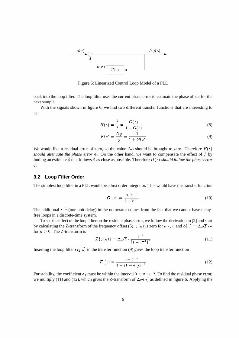
Figure6: LinearizedControlLoop Modelof a PLL

backinto theloopfilter. Theloop filter usesthecurrentphaseerrorto estimatethephaseoffsetfor thenext sample.

With thesignalsshown in figure6, we find two differenttransferfunctionsthatareinterestingtous: n.�*g��h# y`` # m{�*g��phb-m{�*g�� (8)| �*g��$# R `` # ppfbcm{�*g�� (9)

We would like a residualerror of zero,so the value R ` shouldbe broughtto zero. Therefore| �*g��

shouldattenuatethe phaseerror`. On the other hand,we want to compensatethe effect of

`by

findinganestimatey` thatfollows`

ascloseaspossible.Thereforen.�*g�� shouldfollow thephaseerror`.

3.2 Loop Filter Order

Thesimplestloopfilter in aPLL wouldbeafirst orderintegrator. ThiswouldhavethetransferfunctionmS} �*g��$# ~ }"g K }pf,�g K } (10)

Theadditional g K } (oneunit delay)in thenumeratorcomesfrom thefact thatwe cannothave delay-freeloopsin adiscrete-timesystem.

To seetheeffectof theloopfilter ontheresidualphaseerror, wefollow thederivationin [2] andstartby calculatingtheZ-transformof thefrequency offset(5).

` ����� is zerofor �a��� and` �����$#�RS9G+.A��

for �Y��� . TheZ-transformis �]� ` �����"�]#&RS9G+-A g K }��pE,.g K } ��� (11)

Insertingtheloop filter mS} �*g�� in thetransferfunction(9) givestheloop transferfunction| }��*g��h# pf,�g K }pE,-��pE, ~ }���g K } (12)

For stability, thecoefficient ~ } mustbewithin theinterval �{� ~ }f��W . To find theresidualphaseerror,we multiply (11) and(12), whichgivestheZ-transformof R ` ����� asdefinedin figure6. Applying the

6

final valuetheoremof theZ-transform,wegetR ` #��Q�Q�'(�]� R ` �����$#)�Q�Q�� � } �*g],-p(��A �]� R ` �����"�V#)�Q�Q�� � } RS9G+ ppf,���pf, ~ }"��g K }R ` # RS9G+~ } (13)

This meansthatwith a first orderloop filter therewill alwaysbea residualerror, which canbemini-mizedby choosing~ } asbig aspossible.

However, the residualerror canbebroughtto zeroby usinga secondorderloop filter. A secondorderfilter hasthetransferfunction m � �*g��$#�~ }g K } b ~ � g K ���pf,�g K } ��� (14)

Thecoefficient rangefor stabilityof theloopwill bediscussedin section3.4. Wefind thelooptransferfunctionby inserting m � �*g�� into (9), whichgives| � �*g��h# ��pf,�g K } � �pE,-��WH, ~ }���g K } b���pfb ~ � ��g K � (15)

Againwedeterminetheresidualphaseby usingthefinal valuetheoremof theZ-transform,R ` #U�Q�Q�� � } � �*g],cp(� RS9G+Hg K }��pE,�g K } ��� ��pE,�g K } � �pf,���WH, ~ }���g K } b&��phb ~ � ��g K ���R ` #&� (16)

Thusif weuseasecondorderloop filter, thereis no residualphaseerrorleft.

3.3 Loop Filter Structure

Themoststraightforward implementationof thesecondordertransferfunction(14)wouldbeaDirect-Form IIR Filter, figure7(a). However, aswill beshown in section5.2, thefilter will be mucheasierto implementif we usea structureasproposedin [3], shown in figure 7(b). This PLL-suitedfilterstructurehasthetransferfunctionm{�*g��$#��0� � g K }pf,�g K } bc�(}�� g K }pE,.g K } (17)

As caneasilybeshown, ~ }h#��(} and ~ � #&� � ,��(} .Note that [3] usesthe indicesof the coefficients �(} and � � the otherway round. Also note that

[3] calls only thefirst producttermof (17) the “loop filter”. In [3], thesecondterm of (17) is called“VCO” (digital VoltageControlled-Oscillator). We won’t follow thoseconventionsbut will call thetransferfunction m{�*g�� the“loop filter”.

7

����/0�23��� 23��� ����/0��(� � �

zf� �(a)TransposedDirect-Form

����/0��"�

23���� � 23��� ����/0�

(b) PLL-suitedstructureaccordingto [3]

Figure7: Possiblefilter structures

3.4 Loop Filter Coefficients

In PLL-relatedliterature[3] it is suggestedto expressthe loop filter coefficients by the two valuesNatural Frequency9 ' #�W X�Z ' q3Z(� andDampingFactor � . Both valuesarereal numbersgreaterorequalto zero,andfor our applicationwe additionallyrestrictthemto be lesseror equalto one. Z(� isthesamplingfrequency of thediscrete-timesystem.

For thecaseof adirectIIR implementationwith transferfunction(14), thecoefficients ~ }�� ~ � wouldbecalculatedasfollows,with Z(� asthesamplingfrequency:

~ }$#�k3X � Z 'Z(� � ~ � #-k3X Z 'Z(� ��X Z 'Z(� ,a�0� (18)

For thecaseof thePLL-suitedfilter structurewith transferfunction(17), thecoefficientsarecalculatedas �(}$#iW �C9 ' #�k3X � Z 'Z(�� � #�9 �' #-k3X � � Z 'Z(� � � (19)

We recall ~ }h#��(} and ~ � #&� � ,��(} .With this equations,9 ' and � aresufficient to describethe loop filter, andwe will examinethe

behavior of theloop only in thoseparameters.

3.5 Stability

To determinetherangeof stabilityfor theloopparameters,weneedtofind thepolesof thelooptransferfunction.Weinsertthecoefficients(19) into thetransferfunction m{�*g�� accordingto (17)whichresults

8

Natural Frequency fn

Dam

ping

Fac

tor η

10−4

10−3

10−2

10−1

100

0

0.2

0.4

0.6

0.8

1

Figure8: Rangeof stability: �¡ -X�Z 'in thefilter transferfunction m{�*g��$# 9 �' g K � b&��pf,�g K } ��g K } W �C9 '��pf,�g K } � � (20)

This filter is insertedin theloop transferfunction| �*g�� from (9), giving| �*g��$# pphb-m{�*g�� # ��pE,�g K } � �phb&��W �C9 ' ,cW3��g K } b&��pf,cW �C9 ' b�9 �' ��g K � (21)

In fact we could usethe transferfunction n.�*g�� from (8) aswell, becauseit will result in the samedenominator. For stability thepolesof thattransferfunction(i.e. thezerosof thedenominator)needtolie insidetheunit circle. We needthefollowing conditionto hold¢ ���C9 ' ,-p(��£&¤ ���C9 ' ,-p(���h,���pf,cW �C9 ' b�9$�' � ¢ �ip (22)

Wecansimplify thetermunderthesquareroot to ,f9 �' ��pG,¥� � � . Because�S¦-�¡¦&p , this termwill notbecomepositive, thusthesquareroot will bepurelyimaginary. Thestabilityconditionbecomes¢ �C9 ' ,cpf£a§(9 ' ¤ pf,.��� ¢ �&p (23)

By squaringthis inequality, we get���C9 ' ,-p(� � b.9 �' ��pf,.� � �$#ipE,�W �C9 ' b.9 �' �&p (24)9 ' ��9 ' ,cW �0�h�-� (25)

andfinally, because9 '  �� , W �¥ c9 ' (26)

9

Expressingthisconditionin Hertzratherthanin Radiansgives�¡ -X�Z ' q3Z(� (27)

Theabsoluterangefor thecoefficientsis limited by �S�-�¡�&p andtherefore�S�&Z ' q3Z(�f�ip(q X . Figure8 shows thevalid rangefor � and Z ' (normalizedto unit samplingfrequency Z(�]#¨p ). Theregion ofstability is shadedgray. Notethatthefrequency axisis scaledlogarithmically.

3.6 Natural Frequenc y

We will now examinetheeffect of thenaturalfrequency on theloop transferfunction. We recall fromsection3.1that

| �*g�� shouldattenuatethephaseerror`, and n.�*g�� shouldfollow thephaseerror

`.

Figures9 and10show themagnitudefrequency responseplot of| �*g�� and n.�*g�� , respectively, withZ ' asparameterin therangeZ ' #ip � K0© j�j�j�ªGA"p � K � . Thesamplingfrequency is assumedunity, Z(�h#Tp .

F(z)

Frequency (rad/sec)

Mag

nitu

de (

dB)

10−4

10−3

10−2

10−1

100

−70

−60

−50

−40

−30

−20

−10

0

10

fn=10−4

10−3

10−2

3⋅10−4

3⋅10−2

3⋅10−3

Figure9: Frequency Response¢ | �*< =�> � ¢ «�¬

H(z)

Frequency (rad/sec)

Mag

nitu

de (

dB)

10−4

10−3

10−2

10−1

100

−70

−60

−50

−40

−30

−20

−10

0

10

fn=10−4

3⋅10−4

10−3 3⋅10−3

10−2 3⋅10−2

Figure10:Frequency Response¢ n.�*< =�> � ¢ «�¬

The power spectraldensityof` �����{#�RS9-A3� +&b ` = ����� , accordingto the Z-transformin (11),

consistsof a double-poleat gi#­p , plus the power spectraldensity (PSD) of the phasejitter, i.e.the randomprocess̀ = ����� . The phasejitter or phasenoise

` = ����� , causedby theanalogfront-end,isgenerallymodeledas low-passfiltered white noise. Thus the magnitudefrequency plot of the PSDlook thesameasfigure10. This is preciselywhatwe want n.�*g�� to do: n.�*g�� shouldfollow thephaseerror

`. On theotherhand,

| �*g�� shouldattenuatethephaseerror, which is whatweseein figure9.ThePSDof low-passnoisecanbespecifiedby thegainat low frequenciesandanoffsetfrequency,

after which the frequency responsewill declineaccordingto p(q3Z � . If we are given suchan offsetfrequency for thePSDof

` = ����� , thenwe shouldchooseZ ' to comeascloseaspossibleto thegivenoffsetfrequency, sothat

¢ n.�*g�� ¢ matchesthePSDof` ����� asgoodaspossible.

However, we cannotmake Z ' arbitrarily big, becausethePLL might getunstable.In simulationswith a single-carriermulti-antennasystem(seesection4.2), the usefulvaluesfor Z ' q3Z(� werein therangeof ªGA"p � K � j�j�j�ªGA"p � K¯® with �[#&�Cj±° , whichis oneorderof magnitudesmallerthanthetheoretical

10

stability boundaryZ ' ���Cj±°3q²0³$#Tp3jO´HA3p � K } . Weassumethatthis is becauseof imperfectionsin otherblocksof thereceiver, whichwereneglectedduringthelinearizationof thecontrolloop(figure6).

In simulationswith amulti-carriersystem(seesection4.3),theusefulvaluesfor Z ' q3Z(� werefoundto be in the rangeof p � K¯® j�j�j p � K0© which is anotherorderof magnitudesmaller. On the otherhanda multi-carriersystemis muchmorecomplicatedthanthesimplified control loop from figure6. Forexample,thephasecorrectionis doneatchiprate,whereasthephaseerrordetectionhappensatsymbolrate which is only a fraction of the chip rate. The derivation in section3.5 doesnot take this intoaccount,andthe Fourier transformationin betweenis ignoredaswell. We think it is reasonabletoreferto simulationsfor finding out therangeof stability for theparameterZ ' .3.7 Damping Factor

We would like to find out theeffect of thedampingfactoron the loop transferfunction. Thenaturalfrequency wasexaminedin the frequency domain,but the dampingfactor is easiervisualizedin thetimedomain.Werecallfrom section3.1that

| �*g�� shouldattenuatethephaseerror`, and n.�*g�� should

follow thephaseerror`.

Figure11showsthestepresponseof| �*g�� , andfigure12showstheimpulseresponseof n.�*g�� , both

with thedampingfactor � asparameterin the range�CjQpGj�j�j��CjOµ . Thesamplingfrequency is assumedunity, Z(�h#Tp , andthenaturalfrequency is chosento be Z ' #&�CjO�Cp .

Step Response f(t)

Time (sec)

Am

plitu

de

0 50 100 150 200−0.8

−0.6

−0.4

−0.2

0

0.2

0.4

0.6

0.8

.7

.5

.3

η=.9

.1

Figure11:StepResponseof| �*g�� (bold: �[#��Cj±° )

Impulse Response h(t)

Time (sec)

Am

plitu

de

0 50 100 150 200

−0.04

−0.02

0

0.02

0.04

0.06

0.08

0.1

0.12

η=.9

.7 .5

.3 .1

Figure12: ImpulseResponseof n.�*g��As we caneasilysee,a greaterdampingfactor resultsin a shortersettlingtime after a transient

change.It is thereforedesiredto choosea big dampingfactor.However, a big � alsohasa drawback.This is shown below in section3.8but canbeseenhereas

well. Namely, noisein the input might not beattenuatedasmuchasdesired.In the impulseresponseplot (figure12)wecanseethatfor �¡#��CjOµ thepeakat !$#&� is muchgreaterthanfor any smaller� . Ifthe input is white noisewith autocorrelationfunction BC����� , thentheoutput(residualphaseerror)willbecloserto white noisefor a big � . For asmaller � thenoisecomponentis moreattenuated.

11

Thereforethe optimal � is somewherearound �i¶4�Cj±° . We will discussthat more in the nextsection.

3.8 Noise Number

Thenoisenumberof a LTI systemwith noisetransferfunction n � �*g�� is defined[2] as· � # pX ¸¹ : ¢ n � �*< =�> _ � ¢ ��º 9G+ (28)

This canbe seenasthe power of the outputrandomprocesswherethe input of the systemis whitenoisewith unit power. It is a measureof how muchthe noisegetsattenuatedor amplifiedby a LTIsystem.

t ��2(�v ��/0�

wv ��/0�u]v ��/0�z v0» ��/0�

Figure13:PLL ControlLoop modelwith phasenoise

For ourPLL controlloop,wefirst needto identify thepointof noiseinputin thesystem.Accordingto thederivation in [2], the phasenoiseis modeledby a noiseinput signalafter theoffset correctionandtheslicer. Thereforethephasenoisesignal

` � ����� is introducedasshown in figure13.Thenoisetransferfunctionin oursystemthenisn � �*g��h# R ` �����` � ����� # ,Hm{�*g��phb-m{�*g�� #T,En.�*g�� (29)

If weevaluate(28)with this transferfunctionfor differentparametersZ ' q3Z(� and � , wecancharac-terizethedependency of thenoisenumberontheparameters.In figure14,weseethenoisenumber(inºC¼ ) asa functionof thedampingfactor � , andwith thenaturalfrequency Z ' asparameter(samplingfrequency Z(�h#Tp ).

Herewe canclearlyseethat thereis someoptimaldampingfactorat approximately�Y¶U�Cj±° . Ontheotherhand,we canalsoseethatthedampingfactorcanbevariedwidely without having too mucheffectonthenoisenumber. Hence,thedampingfactorgivesussomedegreeof freedomwhenchoosingthefilter coefficients.

As anaside,for thecaseof a first orderloop filter (10) thedependency of thenoisenumberon thefilter coefficient is shown in in figure15. We saw from (12) that the stability is limited to the range�.� ~ }[�½W . From figure 15 we seethat the coefficient ~ } betterbe smallerthan ¶½�CjO¾ . Sincewestatedthat ~ } shouldbeasbig aspossible,this factunderlinesonceagainthatasecondorderloopfilteris neededfor thePLL.

12

0 0.2 0.4 0.6 0.8 110

−3

10−2

10−1

100

101

Damping factor η

Pz

fn=3e−2

fn=1e−2

fn=3e−3

fn=1e−3

fn=3e−4

Figure14: NoiseNumberfor secondorderloop filter

0 0.2 0.4 0.6 0.8 1 1.2 1.4 1.6 1.8 2

10−2

10−1

100

101

102

Coefficient a1

Pz

Figure15:NoiseNumberfor first orderloopfilter

13

3.9 Phase Error Detection

We determinethecurrentphaseerrorby a phasecomparisonbetweenthereceivedsymbols IJ ����� andsomereferencesymbols.Thosereferencesymbolscanbeobtainedcontinuouslyin anumberof differ-entways,namelyby¿ pilot symbolsalternatingwith datasymbols,¿ pilot carriersin amulti-carriersystem(e.g.OFDM)¿ makinga hard-decisionon thereceivedsymbols(“decision-directed” mode)

It is thespecificationof anactualtransmissionsystemwherethepreferredmethodis chosen.SincetheBWRC hasnot yet specifieda MCMA systemat this point in time, we werenot ableto optimizethePLL for a particularchoiceof referencesymbols.

However, someof theMEA algorithmsunderconsideration(especiallySVD) work in a decision-directedmode. This meansthat the systemalreadyincludescircuitry to make a hard-decisiononthe received symbols. For this casewe recommendusing thoseavailable symbolsfor a decision-directedPLL aswell. Thereforetheexamplesin section4.2and4.3useadecision-directedphaseerrordetection.

We would like to discussthe detectionof a phasedifference. Given a received symbolJ

andareferencesymbol º , thestraightforward implementation for thephasedifferencewould beR ` #&À(Á � J A º�à �H#&À(Á � ¢ J º ¢ A(<�=�N±d Ä K d�Å�P�]# `¯Æ , ` «

(30)

This would requirea complex multiplicationanda Cartesian-to-polarconversion.If we consideronlythephaseoffsetin thereceivedsymbol,wecanwrite it as

J # º < =^�d . Thenwecangetrid of thepolarconversionby thefollowing approximationÇ3È � J A º à �¢ º ¢ � # Ç3È � º < =^�d A º à �¢ º ¢ � #�É�QÊ��*R ` �h¶�R ` (31)

This approximationis valid for small phaseoffsets,which is the rangeof operationanyway. Bothmethodsareimplementedasa SIMULINK block in thelibrary describedbelow in section4.4.

Furthersimplificationsof thiswould involve choosingspecialreferencesymbols,for exampleº #p , which would resultin thephaseerrordetectionassimpleas R ` # Ç3È � J � . As statedbefore,thisdoesnot take amplitudevariationsof

Jinto account. It requiresfurther investigationto choosethe

appropriatephasedetectionalgorithmdependingon theactualsystemspecification.

14

V†V

σ1

Uσ4

U†

'x 'y

z'1

z'4

Tx RxChannel

yx

φje

φ̂je−

Figure16:SVD System

4 Application

4.1 Single-carrier SVD

Thefirst applicationof a frequency offset trackingPLL wasdonein themodelfrom [4]. Themodelexistsonly in MATLAB code.Theoverall structureis shown in figure16. As mentionedin section3.9,thePLL is working in decision-directed modebecausetheSVD algorithmworksdecision-directedaswell. For anexplanationof theSVD algorithmwereferto [4], [1].

We note a particularity of the SVD algorithm, namely, that the Ë tracking block is inherentlyimmuneto any phaseoffset. The trackingof the Ë matrix dependsonly on the spatialautocorrela-tion of the datasymbols. Sincethe vectorof symbolsfrom all the antennasis received at onepointin time, all symbolshave the samephaseoffset. Thus the spatialautocorrelationmatrix Ì Æ �����¡#}ÍcÎ 'ϱР' K ÍhÑ } J ��³� J�Ò ��³� is independentof any instantaneousphaseoffset2. Thatmeanswecanfreelychoosewhetherthephaseoffsetcorrectionshouldhappenbeforeor after the Ë tracking. In figure16we choseto do thatafterthe Ë tracking.

In [1] it wasmentionedthat a SVD system(thoughadditionallyin a multi-carrierconfiguration)was not able to copewith a frequency offset of more than a fraction of W[A p � K¯Ó of the samplingfrequency (symbol rate, i.e. after FFT). This doesnot comeasa surprisesincethe SVD algorithmitself doesnot take any phaseoffset into account.

Figure28 (at theendof this document)shows thateffect. We canseethatthealgorithmcantrackthe channelmatrix for sometime, but eventuallythe phaseoffset becomestoo big andthe “Error inestimatedH” grows beyondusefulbounds.As mentionedbefore,thetrackingof the Ë matrix (“LeftSingularVectors”) still works fine even thoughthe phaseoffset prohibits tracking of the Ô matrix(“Right SingularVectors”).Thesesimulationswererun with parametersasshown in table1.

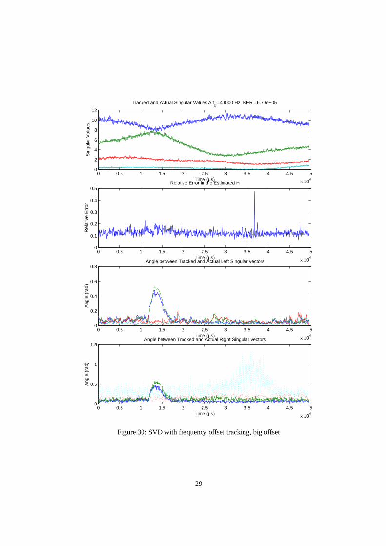
Samplingfrequency 1 MHzConstellation adaptive, from BPSKto 16-PSKSignal-to-Noiseratio 10dBFrequency offset small: 50Hz,medium:1kHz,big: 40kHzPhasenoise nonePLL parameters Z ' q3Z(�h#ip � K � �G�[#&�Cj±°

Table1: Parametersfor SVD simulation2Thereceivedsymbolsonly occurin theterm Õ�ÖQ×�Ø*Õ ÙGÖQ×�Ø where Õ�ÖQ×�Ø is thevectorof symbolsfrom antennaÚ�ÛÛ�Û�Ü at time

instant× .15

After theinclusionof a PLL theperformancewasmuchbetter, seefigure29. In thatgraphwe seethat the channelmatrix is continuouslytracked andthe error remainsmoreor lessconstant¶½�CjQp(° .Thereis onepeculiarity that needssomeexplanation: At the time instant !¥#Ýp3j±° Þ ; the Ë and Ômatrix show a significanterror(“Right” and“Left SingularVectors”).But this is not anerror, insteadit is causedby two singularvaluescomingrathercloseto eachother. The singularvectorsfor thosealmostequalsingularvaluescannotberesolved(thusshowing a largeerror),but thisdoesnot impactthetransmissionquality.

Anotherfactneedssomeexplanation:The“Right SingularVector” plotshasonedottedline thatshows a large error. This is dueto the fact that the smallestsingularvalueis too small to carry anyinformation.Thereforewecannotmakeadecisiononits databits,andbecauseof thislackof referenceinformationit is not possibleto tracktherespective singularvector.

Simulationsin MATLAB showed that the systemwasworking reliablefor offsetsin the orderofp � K � of thesymbolrate(figure29). Evenwith offsetsasbig as °EA�p � K � (which is probablyoutsideofany reasonablespecification)thesystemwasstill working,seefigure30.

We concludethat if the SVD algorithmis augmentedby a PLL, it works asdesiredeven in thepresenceof a reasonablefrequency offset.

4.2 Single-carrier MMSE-QRD

In [5] a multi-antennasystembasedon the minimum meansquaresolution for combiningmultipleantennasis described.At theBWRC,anotherstudenthascreateda SIMULINK modelthat is basedonthepaper[5]. We addedthefrequency offset trackingblock from thelibrary describedin section4.4.Thesystemis shown in figure17.

Out1

Transmitter

received

decided

Out

enable

MEA Receiver

y_from_antenna

received_x

decided_x

corrected_y

phi

Frequency offset tracking (single−carrier

multi−antenna)

received

enable

desired

Detect SNR

In1 Out1

Channel incl. frequency offset

Figure17:MMSE-QRDSystem.Darkgray: MMSE-QRDsystem.Light gray: PLL.

As expected,thePLL increasedtherangeof ausablefrequency offsetgreatly. Figure18shows theSNR for thesymbolsafter MMSE combiningwithout offset tracking. This SNR shouldcomecloseto thechannelSignal-to-Noiseratio which waschosenª3� ºC¼ here.We canseethatwithout tracking,evenasmalloffsetwill significantlydecreaseperformance.With offsettrackingandreasonableerrors,theperformanceis indistinguishablefrom thecasewith no frequency offset.

If the frequency offset is big, the phasetrackingcircuit needsmoretime to converge. We wouldlike to avoid that caseandwould ratherrecommendto add or improve an initial offset acquisitionalgorithm.

Theparametersof thesesimulationsareshown in table2. Thereis notiming/frequencyacquisition

16

0 100 200 300 400 500 600 700 800 900 10000

5

10

15

20

25

30

Ave

rage

SN

R

Symbols

Small error with trackingNo frequency offsetBig error with trackingSmall error, no tracking

Figure18:SNRof theMMSE Systemin variousconfigurations

in this model,but if therewere,we couldview thefrequency offsetof thesesimulationsasa residualerrorof someinitial offsetestimate.

We concludethattheMMSE-QRDalgorithmwill work fine in thepresenceof frequency offset ifthesystemincludesa PLL.

Samplingfrequency 1 MHZIntendedcarrierfrequency ˜2.4GHzConstellation QPSKSignal-to-Noiseratio 30dBFrequency offset small: 1kHz (i.e. 0.5ppm),big: 10kHz(5ppm)Phasenoise ,]p �3� ºC¼ � up to 2.5MHz, thendecreasingas p(q3Z �PLL parameters Z ' q3Z(�h#ip � K � �$�[#&�Cj±°

Table2: MMSE-QRDsimulationparameters

4.3 Single-antenna OFDM

Somestudentsof theBWRChavecreatedanOFDM transmissionsystemmodel[6] in SIMULINK. Weusedthismodelto testthePLL implementationin amulti-carriersystem.TheOFDM systemincludeda timing and frequencyacquisitionblock. The initial frequency offset estimatefrom the acquisitionblock is usedby thePLL asaninitial value.

In somepacket-basedOFDM systems,e.g. IEEE 802.11aor HiperLAN, this initial estimateisassumedto bea sufficient estimateof thefrequency offsetfor thewholetransmissiontime. Thereforethosestandardsdo not requirea trackingcircuit. However, this assumptionis only valid for a limitedtransmissionduration,i.e. packet-baseddatatransfer. But the BWRC is planningto useOFDM inconjunctionwith MEA algorithms[1], andthosealgorithms(especiallySVD) aremuchmoresuited

17

for a continuoustransmissionmodethanfor packet-baseddatatransfer3. Thereforewe believe thatsometrackingof thefrequency offsetwill benecessaryto geta multi-carriermulti-antennasystemtowork.

tx_data

raw_bits

Transmitter

In

enable_demod

data

synch

angle

Timing, frequencyAcquisition

In1

Out1

delta_phi

Receiver: FFT, Channel correctionDemodulation, Phase error detection

data

enable_tracking

angle

delta_phi

data_out

Phase tracking & correction

In Out

Channel incl. Fading,

frequency offset, and phase noise

Figure19:OFDM Systemwith DPLL

20 40 60 80 100 120−3.5

−3

−2.5

−2

−1.5

−1

−0.5

0

0.5

Pha

se E

rror

[rad

]

Symbols

small error, trackingMedium error, trackingBig error, trackingSmall error, no trackingMedium error, no tracking

Figure20: Phaseerrorof theOFDM Systemin variousconfigurations(symbolrate)

Figure19 shows theoverall system.Thesimulationparametersarelisten in table3. Theresidualphaseerror, averagedover all carriers,is shown in figure20. This residualphaseerror is detectedatsymbolrate.For thenon-trackingcasewecanseethatthephaseerroraccumulates,sothateventuallyitis impossibleto make a correctdecision.Notethatthis is preciselythesituationof e.g.IEEE 802.11a,but in thatstandardthemaximumtransmissiondurationis chosenshortenoughsothattheaccumulatedphaseerrordoesnot yetprohibit a successfuldemodulation.

Theothercurvesin figure20 show thatwith a PLL, theresidualphaseerror is almostnegligible.Thecurve with a “big error” shows a nonnegligible settlingtime, but this not meantto bea tolerablesettlingtime in somespecification— it is ratheranexamplethatevenif theinitial erroris outsidethespecification,thePLL will notgounstable.

3E.g. becauseof long trainingintervalson theorderof 100symbols

18

Samplingfrequency ß(à3áTâoãIntendedcarrierfrequency ä�åOæ�ç]âoãNumberof carriers 64 (48data,4 pilot)Cyclic prefix length 16 samples( àCåOæ(è�é )Chip duration ê(ë3ß(à3áTâoã[ìiä(à(í�éOFDM symbol(frame)duration î3è�é (80chips)Timing/frequency acquisition Preambleaccordingto IEEE 802.11aConstellation QPSKSignal-to-Noiseratio 40dBFrequency offset 116kHz (i.e. 20ppm)Phasenoise ï]ê à3à(ðCñSò up to 2.5MHz, thendecreasingas ê(ë3ó¯ôError in initial estimate Small: 0.5%, medium: 1%, big: 5%, very big: 10% of the

116kHzfrequency offset,respectivelyPLL parameters ó(õCë3ó(öhì&÷CåQêEø3ê à�ù0ú3û$ü[ì�àCå±äiý ò(þhì&ß3ù¯ÿ(ûhò ô ìiß3ù þ��

Table3: OFDM simulationparameters

500 1000 1500 2000 2500 3000

−0.12

−0.1

−0.08

−0.06

−0.04

−0.02

0

0.02

0.04

Pha

se in

crem

ent

Chip

Actual incrementVery big errorBig errorSmall error

Figure21: Phaseincrement(chip rate)with acquisitiontime in thebeginning

19

Figure21 shows thephaseincrementper chip (i.e. beforeFFT). Thechip rateis æ3à timeshigherthanthe symbolrate. We seethe phasenoise(light gray) dominatingthe figure. The tracked phaseincrement,however, staysat the expectedvalueof the phasenoise,which is what is necessaryfor astablemodeof operation.Evenwith a very big initial error thephaseincrementeventuallyconvergesto the desiredvalue. Again, this is not supposedto be the normalmodeof operation,but it shouldrathershow thatthePLL doesnotgounstableif theinitial erroris outsidethespecification.

Weincludedhereanadditionalfeaturethatis proposedin [2], namely, anadditionalloopfilter andphaseoffsetcorrectionafter theFFT (seefigure25). [2] proposesto usea first orderloop filter offsetcorrectionafter the FFT for each subcarrier independently. We canview that asa form of channeltrackingandchannelcorrectionratherthanplain frequency offset tracking. Thebenefitof this is canbe seenin figure 22(a) which shows the received symbolsin the constellationdiagramof a QPSKmodulation. Without the after-FFT phasecorrection,the constellationlooks like in figure 22(b). Infigure22(b)somepointsshow a(herecounter-clockwise)rotationout of thedesiredplace,whereasinfigure22(a)this rotationis compensatedfor.

−1.5 −1 −0.5 0 0.5 1 1.5−1.5

−1

−0.5

0

0.5

1

1.5

Re

Im

(a)With post-FFTphasecorrection

−1.5 −1 −0.5 0 0.5 1 1.5−1.5

−1

−0.5

0

0.5

1

1.5

Re

Im

(b) No post-FFTcorrection

Figure22: QPSKconstellationdiagram

However, the benefitversusthe implementationcomplexity remainsto be checked in an actualsystemspecification.Additionally, thesystemmodelusedheredid not includeany channeltracking4.As soonas thereis someother algorithm to track the channelvariations(e.g. someof the MEAalgorithms),the benefitof this additionalphasecorrectionmight becomenegligible, andthe systemshouldbetterdowithout it.

In section5.2 we will show that the loop filter coefficients(andthus, ó(õ and ü ) shouldbechosenfrom a setof discretevalues. We calculatedthe varianceof the detectedphaseerror ��ô for variousdiscretevalues. It turnedout that the variance(i.e. noise)of the phaseerror in a systemwith offsettrackingwasalwaysgreaterthanthe phaseerror variance��ô� in the referencesystem.The reference

4This systemassumedtheinitial channelestimatefrom thepreambleto beconstantfor thewholetransmission duration.

20

systemdid not useoffset trackingbut includeda perfect initial offset estimate,i.e. a perfectoffsetcorrection.Figure23 shows theratio of the trackingphaseerrornoiseto the ideal phaseerrornoise,��ô ë���ô� . We ran a numberof simulations(eachmarker for oneoutcome). The solid line shows theaverage.Wecanseethattheminimumphasenoiseoccursat thevaluesü[ì&àCå±ä , ó(õSì�÷CåQê�ø�ê à ù0ú . Notethat if therewereanadditionalscalingfactorin thePLL accordingto section5.1,we would have hadto choosedifferentdiscretevalues.

2 3 4 5 6 7 8 9

x 10−4

1

1.5

2

2.5

3

3.5

fn/f

s

σ2 /σ02

Figure23:Phaseerrorpower (normalizedby theerrorpowerwith idealcorrection)

WeconcludethatanOFDMsystemwith alongtransmissiondurationor in continuoustransmissionwill needa frequency offset trackingcircuit. Thesecondorderloop filter shown in this simulationissufficient to correctthe frequency offset. An additionalphasecorrectionafter FFT canimprove thechannelestimate,but channeltrackingalgorithmsdifferent thanthe oneusedheremight not benefitfrom thispost-FFTcorrection,thusit couldbeleft out.

4.4 Simulink Bloc k Librar y

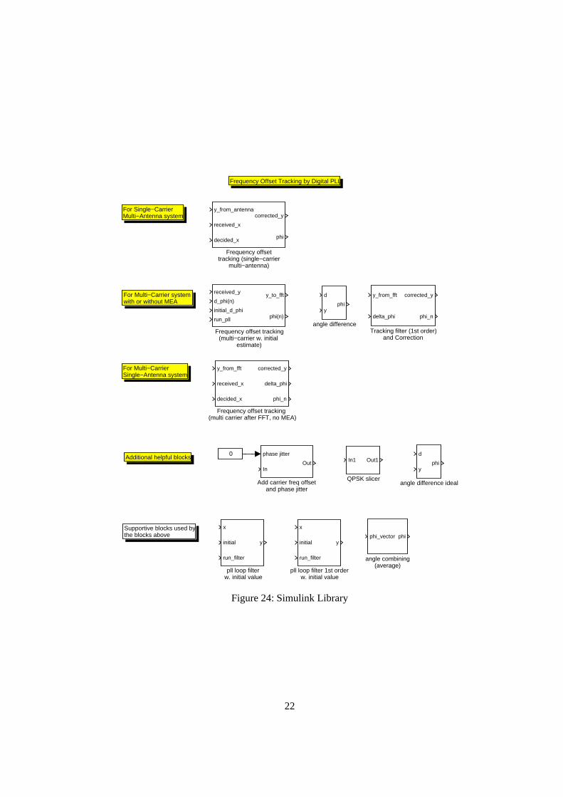
The SIMULINK library shown in figure24 is the collectionof theblocksusedin the above sections.As statedbefore,at the time of writing therewas no multi-carrier multi-antenna(MCMA) systemcompletedyet. The blocks in this library weretestedin a multi-antennasystem(section4.2) andamulti-carriersystem(4.3).

The intendedusageof the blocksin a MCMA systemis shown in figure 25. Thereis oneblockfor thePLL beforeFFT (“Frequency offsettracking”), oneblock right afterFFT (“Trackingfilter (1storder)”), andoneblock after MEA andchannelcorrectionto detectthe currentphaseerror (“angledifference”).Notethatthechannelcorrectionandthefirst ordertrackingfilter canbeinterchanged—thereis no requiredorderfor thesetwo blocks.Additionally, in a single-antennasystem,thepost-FFTtrackingfilter andthephaseerrordetectioncanbesimplifiedinto oneblock,which is the“Frequencyoffsettracking(afterFFT, noMEA)” block.

21

For Single−Carrier Multi−Antenna system

Frequency Offset Tracking by Digital PLL

For Multi−Carrier system with or without MEA

For Multi−CarrierSingle−Antenna system

Additional helpful blocks

Supportive blocks used bythe blocks above

x

initial

run_filter

y

pll loop filter 1st orderw. initial value

x

initial

run_filter

y

pll loop filterw. initial value

d

yphi

angle difference ideal

d

yphi

angle difference

phi_vector phi

angle combining(average)

y_from_fft

delta_phi

corrected_y

phi_n

Tracking filter (1st order)and Correction

In1 Out1

QPSK slicer

y_from_fft

received_x

decided_x

corrected_y

delta_phi

phi_n

Frequency offset tracking (multi carrier after FFT, no MEA)

received_y

d_phi(n)

initial_d_phi

run_pll

y_to_fft

phi(n)

Frequency offset tracking(multi−carrier w. initial

estimate)

y_from_antenna

received_x

decided_x

corrected_y

phi

Frequency offset tracking (single−carrier

multi−antenna)

0 phase jitter

InOut

Add carrier freq offsetand phase jitter

Figure24:Simulink Library

22

1

symbols

d

yphi

angle difference

tx_data

Transmitter

y_from_fft

delta_phi

corrected_y

phi_n

Tracking filter (1st order)and Correction

In

data

angle

synch

Timing, frequencyAcquisition

In1 Out1

MEA processing

In1 Out1

Hard−decision

received_y

d_phi(n)

initial_d_phi

run_pll

y_to_fft

phi(n)

Frequency offset tracking(multi−carrier w. initial

estimate)

In1 Out1

FFT

In Out

Channel incl. Fading,

frequency offset, and phase noise

In1 Out1

Channel Correction

Figure25: Proposedmulti-antennaOFDM system.Light gray: PLL blocks,darkgray: OFDM/MEAblocks

The “Frequency offset tracking” blockstake threearguments:Thenormalizednaturalfrequencyó(õCë3ó(ö , thedampingfactor ü , andthesamplingtime�

. Wereferto sections3.6,3.7,and5.2onhow tochoosethose.

Note that it is still unclearwhetherthe post-FFTcorrectionblock (“Trackingfilter (1st order)”)givesenoughbenefitin theactualsystemto justify its implementation.As statedin section4.3, thatblock might beleft outcompletely.

Furthernotethat therearetwo differentblocksfor the angledifferencedetection.The onesug-gestedto beused(“angledifference”)implementstheapproximationfrom (31). However, for refer-enceit might be usefulto have an ideal differencedetectionlike in (30). This is implementedin theblock “angledifferenceideal” andmight beusefulfor evaluationpurpose.

23

����� �������

��� ���������� �

Figure26:PLL ControlLoop modelwith additionalscalingfactor

5 Fix-Point Implementation

5.1 Scaling Factor

In thefix-point implementationwe have to payextra attentionto possibleotherscalingfactorsin thePLL loop. For example,if thephasecorrectionis doneby a CORDIC,thenthe input angleis scaledby somefixedvaluethatdependson thelookup-tablevaluesof theCORDIC.

Figure26 shows a PLL modelthat takesanadditionalscalingfactorinto account.Insteadof thetransferfunction ç��*ã�� , we now have a scaledloop filter andtheoverall transferfunction is �{ø3ç����*ã�� .If wearegiventheoriginal filter coefficients ò(þ�û"ò ô from (17), wecanfind thescaledcoefficientsasò � þ ì&ò(þ"ë��¯û ò � ô ì�ò ô ë�� (32)

In section5.2,we aregivena discretesetof coefficients ò � þ û"ò � ô , anda scalingfactor � that is fixed(e.g. by theCORDIC).We would like to find out thepossiblevaluesfor thenaturalfrequency ó(õCë3ó(öandthedampingfactor ü . By inserting(32) into (19) andsolvingfor ó(õ and ü , wefindó(õó(ö ì � ò � ôß�! " � (33)ü[ì ò � þß � ò � ô " � (34)

In thefollowing wewould like to statethedependency of ó(õ and ü onthefilter coefficients.Theaboveequations(33), (34) show that we cando that independentlyof the scalingfactor � by only talkingaboutthecoefficientsin termsof ó(õCë " � and ü0ë " � .

5.2 Discrete Coefficients

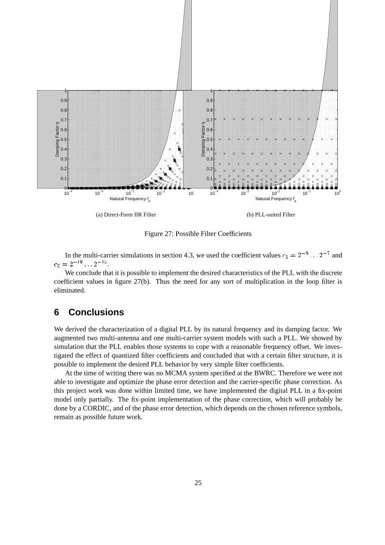
ThePLL in [3] givesanunusualstructurefor a secondorderfilter. But it turnsout thatthisstructureismuchbettersuitedto implementverysimplecoefficients.Thesimplestcoefficientsto beimplementedareinteger powersof two, e.g. ß3ù�#(û�ß3ù0ú3û�ß3ù�$�å�å�å Figure27(a)and27(b) show the possiblevaluesofó(õCë " � and ü0ë " � that could be implementedaspowersof two whenusingeithera direct-formIIRfilter or thePLL suitedstructure,respectively. Therangeof stability is shadedgray.

Obviously thedirect-formdoesnotallow any coefficientsin thestableregionatall. ThePLL suitedstructure,however, shows a regularpatternof usablecoefficients.As shown in section3.8,at leastthedampingfactorcanbevariedwidely.

24

Natural Frequency fn

Dam

ping

Fac

tor η

10−4

10−3

10−2

10−1

100

0

0.1

0.2

0.3

0.4

0.5

0.6

0.7

0.8

0.9

1

(a)Direct-Form IIR Filter

Natural Frequency fn

Dam

ping

Fac

tor η

10−4

10−3

10−2

10−1

100

0

0.1

0.2

0.3

0.4

0.5

0.6

0.7

0.8

0.9

1

(b) PLL-suitedFilter

Figure27:PossibleFilter Coefficients

In themulti-carriersimulationsin section4.3,weusedthecoefficient valuesò(þ$ìiß ù¯ÿ å�å�å�ß ù�% andò ô ì&ß ù þ ÿ å�å�å�ß ù þ $ .Weconcludethatit is possibleto implementthedesiredcharacteristicsof thePLL with thediscrete

coefficient valuesin figure 27(b). Thus the needfor any sort of multiplication in the loop filter iseliminated.

6 Conc lusions

We derived thecharacterizationof a digital PLL by its naturalfrequency andits dampingfactor. Weaugmentedtwo multi-antennaandonemulti-carriersystemmodelswith sucha PLL. We showed bysimulationthat thePLL enablesthosesystemsto copewith a reasonablefrequency offset. We inves-tigatedtheeffect of quantizedfilter coefficientsandconcludedthatwith a certainfilter structure,it ispossibleto implementthedesiredPLL behavior by very simplefilter coefficients.

At thetimeof writing therewasnoMCMA systemspecifiedat theBWRC.Thereforewewerenotableto investigateandoptimizethephaseerrordetectionandthecarrier-specificphasecorrection.Asthis projectwork wasdonewithin limited time, we have implementedthe digital PLL in a fix-pointmodelonly partially. The fix-point implementationof the phasecorrection,which will probablybedoneby aCORDIC,andof thephaseerrordetection,whichdependsonthechosenreferencesymbols,remainaspossiblefuturework.

25

7 Ackno wledgments

Theauthorwould liketo thankhisfellow studentsNing Zhang,JosieAmmer, andAdaPoonfor fruitfuldiscussions.

References

[1] A.G. Klein, TheHornetRadioProposal:A Multicarrier, Multiuser, MultiantennaSpecification.Ph.D.thesis,UC Berkeley 2000

[2] K.D. Kammeyer. Nachrichtenübertragung [in German].TeubnerVerlag, Stuttgart,Germany,1996

[3] Y.R.Shayan,T. Le-Ngoc.All digital phase-locked loop: concepts,designandapplications.IEEEProc.,Vol. 136,Pt.F, No. 1, February1989.

[4] A.S.Y. Poon,D.N.C.Tse,andR.W. Brodersen,An adaptive multi-antennatransceiver for slowlyflat fadingchannels.To appearin IEEE Trans.onCommunications, 2001

[5] B. Haller. DedicatedVLSI Architecturesfor adaptive Interferencesurpressionin WirelessCom-munication systems.In: Circuits and Systemsfor WirelessCommunications, ETH Zurich,Switzerland.

[6] Y. Chiu,D. Markovic, H. Tang,N. Zhang.OFDM ReceiverDesign.FinalReportfor ClassProjectEE225C.Fall 2000.

26

0 0.5 1 1.5 2 2.5 3 3.5 4 4.5 5

x 104

0

5

10

15Tracked and Actual Singular values

Time (µs)

Sin

gula

r V

alue

s

0 0.5 1 1.5 2 2.5 3 3.5 4 4.5 5

x 104

0

0.5

1

1.5

2Relative Error in the Estimated H

Time (µs)

Rel

ativ

e E

rror

0 0.5 1 1.5 2 2.5 3 3.5 4 4.5 5

x 104

0

0.2

0.4

0.6

0.8Angle between Tracked and Actual Left Singular Vectors

Time (µs)

Ang

le (

rad)

0 0.5 1 1.5 2 2.5 3 3.5 4 4.5 5

x 104

0

0.5

1

1.5

2Angle between Tracked and Actual Right Singular Vectors

Time (µs)

Ang

le (

rad)

Figure28:SVD without frequency offsettracking,smalloffset

27

0 0.5 1 1.5 2 2.5 3 3.5 4 4.5 5

x 104

0

2

4

6

8

10

12

Tracked and Actual Singular Values. ∆ fc =1000 Hz, BER =2.07e−04

Time (µs)

Sin

gula

r V

alue

s

0 0.5 1 1.5 2 2.5 3 3.5 4 4.5 5

x 104

0.05

0.1

0.15

0.2

0.25Relative Error in the Estimated H

Time (µs)

Rel

ativ

e E

rror

0 0.5 1 1.5 2 2.5 3 3.5 4 4.5 5

x 104

0

0.2

0.4

0.6

0.8Angle between Tracked and Actual Left Singular vectors

Time (µs)

Ang

le (

rad)

0 0.5 1 1.5 2 2.5 3 3.5 4 4.5 5

x 104

0

0.5

1

1.5

2Angle between Tracked and Actual Right Singular vectors

Time (µs)

Ang

le (

rad)

Figure29: SVD with frequency offsettracking,mediumoffset

28

0 0.5 1 1.5 2 2.5 3 3.5 4 4.5 5

x 104

0

2

4

6

8

10

12

Tracked and Actual Singular Values. ∆ fc =40000 Hz, BER =6.70e−05

Time (µs)

Sin

gula

r V

alue

s

0 0.5 1 1.5 2 2.5 3 3.5 4 4.5 5

x 104

0

0.1

0.2

0.3

0.4

0.5Relative Error in the Estimated H

Time (µs)

Rel

ativ

e E

rror

0 0.5 1 1.5 2 2.5 3 3.5 4 4.5 5

x 104

0

0.2

0.4

0.6

0.8Angle between Tracked and Actual Left Singular vectors

Time (µs)

Ang

le (

rad)

0 0.5 1 1.5 2 2.5 3 3.5 4 4.5 5

x 104

0

0.5

1

1.5Angle between Tracked and Actual Right Singular vectors

Time (µs)

Ang

le (

rad)

Figure30:SVD with frequency offsettracking,big offset

29