free vibration analysis of repetitive structures using...

1 (1), 27-35, Spring 2011

19

Journal of Structural Engineering and Geotechnics, 2(1), 19-28, Winter 2012

QIAU

Free Vibration Analysis of Repetitive Structures using Decomposition, and Divide-Conquer Methods

L. Shahryari

Science and Research, Fars Branch, Islamic Azad University, Fars, Iran

Received 21 Dec, 2010; Accepted 4 Jan, 2011

Abstract

This paper consists of three sections. In the first section an efficient method is used for decomposition of the canonical matrices associated with repetitive structures. to this end, cylindrical coordinate system, as well as a special numbering scheme were employed. In the second section, divide and conquer method have been used for eigensolution of these structures, where the matrices are in the block tri-diagonal form. In the third section a comparison of the results is presented. In order to illustrate the efficiency of the aforementioned methods, repetitive structures are considered in the form of barrel vault space structures. Keywords: Space structures (barrel vaults), Factor analysis, Eigenvalues and Eigenfunctions, Vibration 1. Introduction

Real symmetric eigenvalue problems frequently arise from scientific and engineering computations. The structures of the matrices and the requirements for the eigensolutions vary by application. For instance, many matrices generated from electronic structure calculations in quantum mechanics have strong locality properties. Some of them are block-tridiagonal; some are dense but with larger elements close to the diagonal and a decrease in the magnitudes of elements as they move from the diagonal. In many situations, the second type of matrices may be approximated by block-tridiagonal matrices with very low computational cost. In this paper two useful and high speed methods were compared to each other in order to solve the eigensolutions.[1-18,19]. There are several applications of eigenproblems in

structural mechanics. The eigenvalues and eigenvectors of graphs play an important role in algebraic graph theory and combinatorial

optimization. Large structural models and their corresponding graphs have large and sparse matrix representations. The factorization of these matrices

* Corresponding Author Email: [email protected]

with arbitrary patterns requires general methods. special topologies the associated matrices of which can be transformed to particular patterns in such a manner that their factorizations can more easily be performed. Some of these matrices were previously studied by Kaveh and Sayarinejad [20-21], Kaveh and Rahami [22], and some other general eigensolution methods are also available in Robbe and Sadkane [23], Park [24], Mathias and Stewart [25] and Hasan and Hasan [26], among many others. There are also some applications of graphs spectra in nodal and element ordering and graph partitioning. Further information about these issues can be found in Gould [27], Straffing [28], Maas [29], and Grimes et al. [30]. However, despite of the efficiency of graphs spectra for combinatorial optimization, the calculation of eigenvalues and eigenvectors of large graphs and their corresponding structural models without considering patterns and the sparsity of their matrices require considerable memory and computational time. In this article, a new canonical form and its relation with some structural models often encountered in practice are presented.

L. Shahryari

20

The block-tridiagonal divide-and-conquer algorithm developed by Gansterer

And Ward et al. [16] provides an eigensolver that addresses the above issues. Their algorithm computes all the eigenvalues and eigenvectors of a block-tridiagonal matrix to reduced accuracy with a similar reduction in execution time for most applications.

One of the challenges is that the matrix sizes are usually very large and exceed the limitation of single processor architecture. Thus, parallel computation becomes necessary. The block-tridiagonal divide-and-conquer algorithm is considered inherently parallel because the initial problem can be divided into smaller subproblems and solved independently. We are thus motivated to implement an efficient, scalable parallel block-tridiagonal divide-and-conquer eigensolver with the ability to compute eigensolutions to a user-specified accuracy.

2. Block Diagonalization of Compound Matrices In linear algebra it is known that a square matrix can be diagonalized using the normalized eigenvectors, provided that all the eigenvectors are orthogonal. It is also proved that if the matrix is Hermitian, then it can be diagonalized and diagonal entries constitute the eigenvalues of this matrix. A matrix is Hermitian if its conjugate is the same as its transpose. Therefore, if a matrix is real, then symmetry is the only requirement to make the matrix Hermitian. The eigenvalues of Hermitian matrices are real and the eigenvectors corresponding to any arbitrary pairs of distinct eigenvalues are orthogonal. If M is a Hermitian matrix, then it can be diagonalized using MUU t . All what is required is the formation of an orthogonal matrix U. This can in fact be achieved by the Singular Value Decomposition (SVD) approach for symmetric matrices. Definition: The Kronecker product of two matrices A and B is the matrix we get by replacing the entry ij of A by ij of B, for all i and j .

As an example,

000001

11

dcba

dcdcbaba

dcba (1)

Where the entry(1,1) in the first matrix has been replaced by a complete copy of the second matrix. Now the main question is how one can block diagonalize a compound

matrix. For a matrix M defined as a single Kronecker product, in the form 11 BAM , it is obvious that if 1A is Hermitian, then the diagonalization leads to a block diagonal matrix of the form 11 BDA . Now suppose a compound matrix M can be written as the sum of two Kronecker products:

2211 BABAM (2)

Now we want to find a matrix P which diagonalizes 1A and 2A . In such a case, one should show that IPU

block diagonalizes M, i.e., we have to show that MUU t

is a block diagonal matrix. From algebra we have t t tA B A B and A B C D A C BD Then: 푈 푀푈 = (푃 ⨂퐼 )(퐴 ⨂퐵 + 퐴 ⨂퐵 )(푃⨂퐼) = [(푃 퐴 ⨂(퐼퐵 ) + (푃 퐴 )⨂(퐼퐵 )](푃⨂퐼) = (푃 퐴 푃)⨂(퐵 퐼) + 푃 퐴 푃)⨂(퐵 퐼) = (푃 퐴 푃)⨂(퐵 ) + (푃 퐴 푃)⨂(퐵 )

(3)

Since it is assumed that P diagonalizes 1A and 2A , 푃 퐴 푃 = 퐷 푎푛푑푃 퐴 푃 = 퐷 (4) Therefore

21 21BDBDMUU AA

T (5) Thus, U becomes block diagonalized, and in order to calculate the eigenvalues of M, one can evaluate the eigenvalues of the blocks on the diagonal. M and

tU MU are similar matrices, since P is orthogonal, thus U is also orthogonal and its inverse is equal to its transpose. Now an important question is whether the assumptions made at the beginning of this section are feasible; i.e., can one always find an orthogonal matrix P, which diagonalizes 1A and 2A are feasible simultaneously. For a matrix to be diagonalizable, it is necessary to be Hermitian. However, for two matrices to be diagonalizable, not only should these two matrices be Hermitian, but these matrices should be commutative; i.e., 1221 AAAA should hold. Theorem 1: Two Hermitian matrices 1A and 2A can be diagonalized simultaneously with an orthogonal matrix if and only if

1221 AAAA (6) A simple proof of this theorem can be found in [2]. Therefore, if 1A and 2A commute with respect to multiplication, then according to Eq. (2) and the Theorem 1,

Journal of Structural Engineering and Geotechnics, 2 (1), 19-28, Winter 2012

21

)])()(([ 22111

BABAeig ii

n

iM

(7)

The ii A for 2,1j is a diagonal matrix

containing all the eigenvalues of jA , and n is the

dimension of the matrix iA . It should be noticed that the

order of the eigenvalues in 1A and 2A is important. The order is the same as obtained after simultaneous diagonalization of the two matrices, which appear on the diagonal of the matrices. As an example, for the special case with IA 1 , it is

obvious that IAIA 22 , and according to theorem 1 we have:

221 BABIM ,

1)(,)])(([ 12211

ABABeig ii

n

iM

(8)

These special cases already shown in the work of Kaveh and Sayarinejad [1].

)](),(

,1,1)(,)])(([ 11

BAeigBAeig

TBTAeig

M

i

n

iM

(9)

It should be noted that here blocks are treated as numbers , i.e., they have the commuting property. In general, one can show that:

mmmn

nm

mm

mm

mn ABAF

A

ABBA

M ,,.

.

n

ii

iin

n

n

n BABAn

inM

1

222

0

1det

(10)

Comparing with Eq. (9), we have Ti . Since

0,1,0FT , therefore, as mentioned before, we have

1cos2

ni

Ti , where ....1 ni

2.1. Stiffness Matrix Calcubation

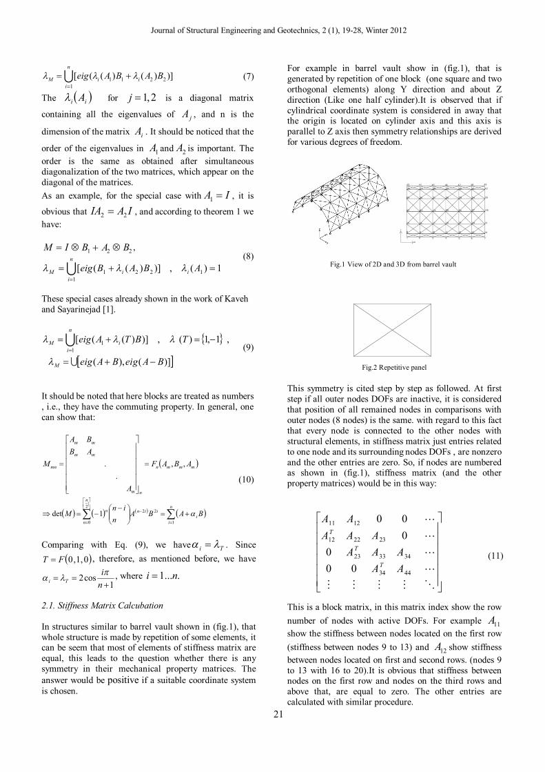
In structures similar to barrel vault shown in (fig.1), that whole structure is made by repetition of some elements, it can be seem that most of elements of stiffness matrix are equal, this leads to the question whether there is any symmetry in their mechanical property matrices. The answer would be positive if a suitable coordinate system is chosen.

For example in barrel vault show in (fig.1), that is generated by repetition of one block (one square and two orthogonal elements) along Y direction and about Z direction (Like one half cylinder).It is observed that if cylindrical coordinate system is considered in away that the origin is located on cylinder axis and this axis is parallel to Z axis then symmetry relationships are derived for various degrees of freedom.

Fig.1 View of 2D and 3D from barrel vault

Fig.2 Repetitive panel

This symmetry is cited step by step as followed. At first step if all outer nodes DOFs are inactive, it is considered that position of all remained nodes in comparisons with outer nodes (8 nodes) is the same. with regard to this fact that every node is connected to the other nodes with structural elements, in stiffness matrix just entries related to one node and its surrounding nodes DOFs , are nonzero and the other entries are zero. So, if nodes are numbered as shown in (fig.1), stiffness matrix (and the other property matrices) would be in this way:

11 12

12 22 23

23 33 34

34 44

0 00

00 0

T

T

T

A AA A A

K A A AA A

(11)

This is a block matrix, in this matrix index show the row number of nodes with active DOFs. For example 11Ashow the stiffness between nodes located on the first row (stiffness between nodes 9 to 13) and 12A show stiffness between nodes located on first and second rows. (nodes 9 to 13 with 16 to 20).It is obvious that stiffness between nodes on the first row and nodes on the third rows and above that, are equal to zero. The other entries are calculated with similar procedure.

L. Shahryari

22

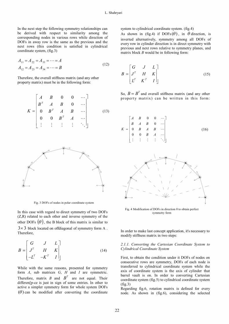
In the next step the following symmetry relationships can be derived with respect to similarity among the corresponding nodes in various rows while direction of DOFs in away row is the same as the previous and the next rows (this condition is satisfied in cylindrical coordinate system, (fig.3)

11 22 33

12 23 34

A A A AA A A B

(12)

Therefore, the overall stiffness matrix (and any other property matrix) must be in the following form:

0 00

00 0

T

T

T

A BB A B

K B A BB A

(13)

Fig. 3 DOFs of nodes in polar coordinate system

In this case with regard to direct symmetry of two DOFs (Z,R) related to each other and inverse symmetry of the other DOFs , the B block of this matrix is similar to

33 block located on offdiagonal of symmetry form A . Therefore,

T

T T

G J LB J H K

L K I

(14)

While with the same reasons, presented for symmetry form A, sub matrices G, H and I are symmetric. Therefore, matrix B and TB are not equal. Their differen[p-ce is just in sign of some entries. In other to active a simpler symmetry form for whole system DOFs

)( can be modified after converting the coordinate

system to cylindrical coordinate system. (fig.4) As shown in (fig.4) if DOFs )( , in direction, is inverted alternatively, symmetry among all DOFs of every row in cylinder direction is in direct symmetry with previous and next rows relative to symmetry planes, and matrix block B would be in following form:

T

T T

G J LB J H K

L K I

(15)

So, TBB and overall stiffness matrix (and any other proper t y matrix) can be wr i t ten in th is form:

0 00

00 0

A BB A B

K B A BB A

(16)

Fig. 4 Modification of DOFs in direction θ to obtain perfect symmetry form

In order to make last concept application, it's necessary to modify stiffness matrix in two steps: 2.1.1. Converting the Cartesian Coordinate System to Cylindrical Coordinate System First, to obtain the condition under it DOFs of nodes on consecutive rows are symmetry, DOFs of each node is transferred to cylindrical coordinate system while the axis of coordinate system is the axis of cylinder that barrel vault is on. In order to converting Cartesian coordinate system (fig.5) to cylindrical coordinate system (fig.3) Regarding fig.6, rotation matrix is defined for every node. As shown in (fig.6), considering the selected


23

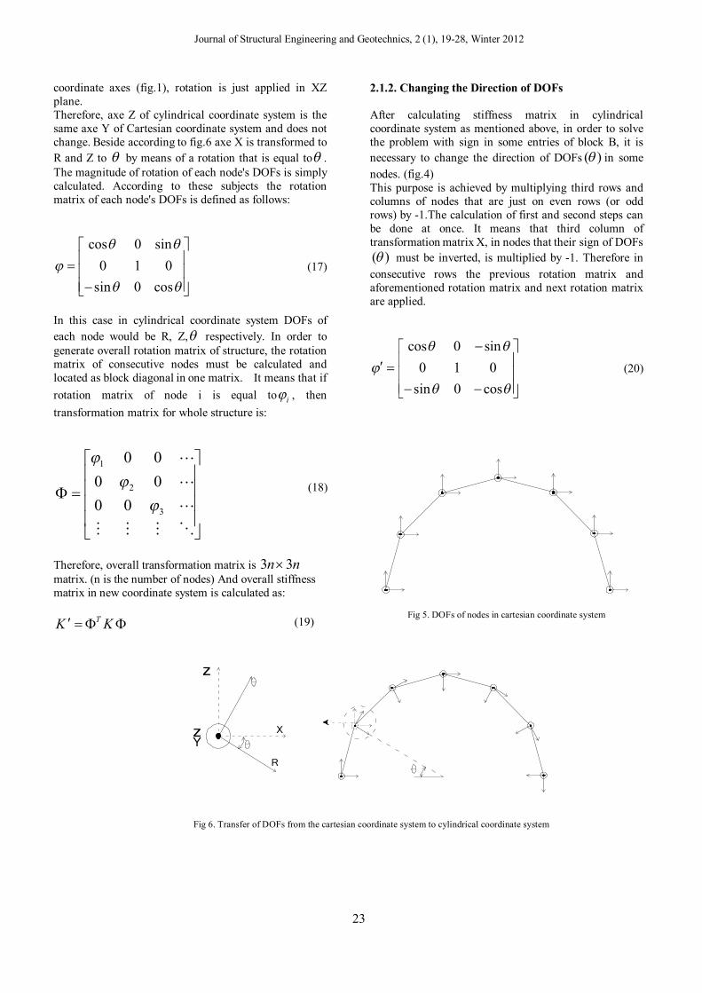
coordinate axes (fig.1), rotation is just applied in XZ plane. Therefore, axe Z of cylindrical coordinate system is the same axe Y of Cartesian coordinate system and does not change. Beside according to fig.6 axe X is transformed to R and Z to by means of a rotation that is equal to . The magnitude of rotation of each node's DOFs is simply calculated. According to these subjects the rotation matrix of each node's DOFs is defined as follows:

cos 0 sin0 1 0

sin 0 cos

(17)

In this case in cylindrical coordinate system DOFs of each node would be R, Z, respectively. In order to generate overall rotation matrix of structure, the rotation matrix of consecutive nodes must be calculated and located as block diagonal in one matrix. It means that if rotation matrix of node i is equal to i , then transformation matrix for whole structure is:

1

2

3

0 00 00 0

(18)

Therefore, overall transformation matrix is nn 33 matrix. (n is the number of nodes) And overall stiffness matrix in new coordinate system is calculated as:

TK K (19)

2.1.2. Changing the Direction of DOFs After calculating stiffness matrix in cylindrical coordinate system as mentioned above, in order to solve the problem with sign in some entries of block B, it is necessary to change the direction of DOFs )( in some nodes. (fig.4) This purpose is achieved by multiplying third rows and columns of nodes that are just on even rows (or odd rows) by -1.The calculation of first and second steps can be done at once. It means that third column of transformation matrix X, in nodes that their sign of DOFs

)( must be inverted, is multiplied by -1. Therefore in consecutive rows the previous rotation matrix and aforementioned rotation matrix and next rotation matrix are applied.

cos 0 sin0 1 0

sin 0 cos

(20)

Fig 5. DOFs of nodes in cartesian coordinate system

z

zY

R

X

Fig 6. Transfer of DOFs from the cartesian coordinate system to cylindrical coordinate system

L. Shahryari

24

3. The Block Tridiagonal Divide-and-Conquer lgorithm

In this section the Block Tridiagonal Divide-and-Conquer (BD&C) algorithm is briefly described.

nn

qq

Tqq

T

T

R

BCCB

CCBC

CB

M

1

11

2

221

11

(21)

where q is the number of diagonal blocks, iB for

qi 1 are the diagonal blocks and iC for

11 qi are the off-diagonal blocks. The BD & C algorithm calculates the eigenvalues of M with a give accuracy tolerance )( mach .

VVM ˆˆˆ

We calculate V̂ and ̂ such that V̂ contains approximations to the eigenvectors of M and the diagonal matrix ̂ contains approximations to the eigenvalues of M.

,ˆˆˆ22

MOVVM T (22)

The product TVV ˆˆ with a small error mach is equal to the unity matrix.

nOeIVV machiT

ni

2,...,2,1ˆˆmax (23)

For ni 1 , ie is the ith column of the unity matrix. The three main steps of the BD&C algorithm are as follows: Problem subdivision, sub problem solution, and synthesis of sub solution. Singular values, singular vectors and their relationship A real positive number is called the singular value of M if and only if the unit vector u in mK and v in nK

exist such that vuManduMv T

12

,~1

11

qifor

VVUUBBi

Tii

i

Tiiii

The vectors u and v are called the left-singular and the right singular for , respectively.

In certain singular decomposition TVUM (24)

The diagonal entries of are equal to the singular values of M, and the columns of U and V are the left singular and right singular vectors corresponding the singular values, respectively.

TVUM (25)

Problem subdivision: The off-diagonal blocks iC are approximated with lower rank matrices using their singular value decompositions:

i

Tii

ij

ij

j

iji VUuC

Ti

1

(26)

In this way the dimension of the matrix iC is reduced.

Where i is the chosen approximate rank of iC , iib

i RU 1 is an orthogonal matrix containing the first

left singular value i and iibi RV 1 contains the first

right singular value, i is a diagonal matrix containing

the largest singular value i of iC for 1,...,2,1 qi . The approximate rank of the off-diagonal blocks in the step corresponding to subdivision of the problem reduces the size of these matrices considering the prescribed approximation; the computational complexity of the calculations is decreased. Using the decomposition the block tridiagonal matrix M can be expressed as a block diagonal matrix.

1

1

ˆq

i

TiiWWMM (27)

Where

qBBBdiagM ~,...,~,~ˆ21 (28)

And

,~1 1111 TVVBB

,~1

11

q

Tqqqq UUBB

(29)


25

and

0

0

,

00

,22

2/1

2/1

2/1

1

2/1

11

1

qifor

U

VWU

V

W

ii

ii

i

2/1

11

2/1

111

00

qq

qqq

U

VW

(30)

Sub Problem Solution

Each diagonal block iB̂ is factorized as

qiforZDZB Tiiii ,...,2,1,ˆ (31)

Then we will have

TZDZM ˆ (32)

Where qZZZdiagZ ,..., 21 is vertical block diagonal

matrix and qDDDdiagD ,..., 21 is a diagonal Note that the traditional algorithms may be applied to compute the eigendecomposition of the diagonal blocks. Typically, the number of diagonal blocks q in a block tridiagonal matrix is much greater than 2 and the block sizes bi are small compared to the matrix size n. Thus, the

Eigen-decomposition of each sub problem iB̂ in Equation (31), which involves only the much smaller diagonal block, yields better data access time pattern than traditional decomposition methods on the much larger full matrix [16]. Here, the node ordering is as the same as what was already described in the first section, the stiffness , mass and geometric stiffness matrices forms are as Equation (16) which by using divide and conquer algorithm can be solved.

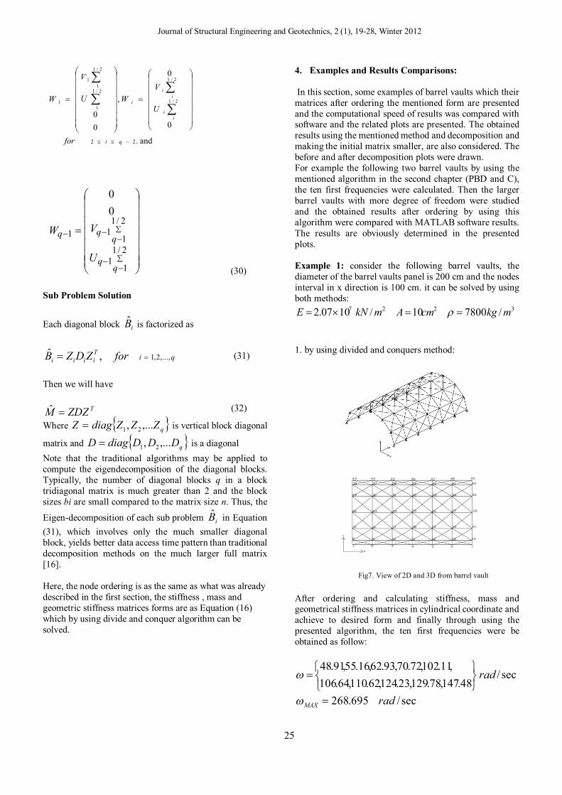
4. Examples and Results Comparisons: In this section, some examples of barrel vaults which their matrices after ordering the mentioned form are presented and the computational speed of results was compared with software and the related plots are presented. The obtained results using the mentioned method and decomposition and making the initial matrix smaller, are also considered. The before and after decomposition plots were drawn. For example the following two barrel vaults by using the mentioned algorithm in the second chapter (PBD and C), the ten first frequencies were calculated. Then the larger barrel vaults with more degree of freedom were studied and the obtained results after ordering by using this algorithm were compared with MATLAB software results. The results are obviously determined in the presented plots. Example 1: consider the following barrel vaults, the diameter of the barrel vaults panel is 200 cm and the nodes interval in x direction is 100 cm. it can be solved by using both methods:

3227 /780010/1007.2 mkgcmAmkNE

1. by using divided and conquers method:

Fig7. View of 2D and 3D from barrel vault

After ordering and calculating stiffness, mass and geometrical stiffness matrices in cylindrical coordinate and achieve to desired form and finally through using the presented algorithm, the ten first frequencies were be obtained as follow:

sec/48.147,78.129,23.124,62.110,64.106

,11.102,72.70,93.62,16.55,91.48rad

sec/695.268 radMAX

L. Shahryari

26

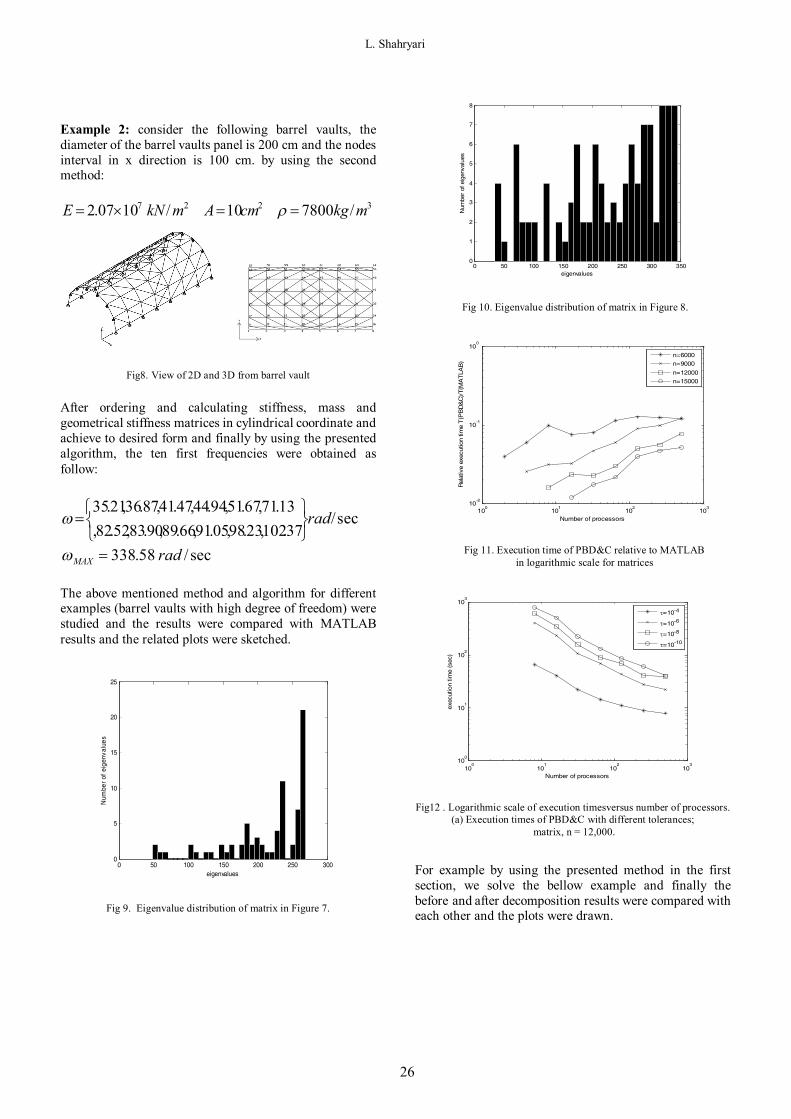
Example 2: consider the following barrel vaults, the diameter of the barrel vaults panel is 200 cm and the nodes interval in x direction is 100 cm. by using the second method:

3227 /780010/1007.2 mkgcmAmkNE

Fig8. View of 2D and 3D from barrel vault

After ordering and calculating stiffness, mass and geometrical stiffness matrices in cylindrical coordinate and achieve to desired form and finally by using the presented algorithm, the ten first frequencies were obtained as follow:

sec/37.102,23.98,05.91,66.89,90.83,52.82,

13.71,67.51,94.44,47.41,87.36,21.35rad

sec/58.338 radMAX

The above mentioned method and algorithm for different examples (barrel vaults with high degree of freedom) were studied and the results were compared with MATLAB results and the related plots were sketched.

Fig 9. Eigenvalue distribution of matrix in Figure 7.


Fig 11. Execution time of PBD&C relative to MATLAB in logarithmic scale for matrices

Fig12 . Logarithmic scale of execution timesversus number of processors. (a) Execution times of PBD&C with different tolerances;

matrix, n = 12,000.

For example by using the presented method in the first section, we solve the bellow example and finally the before and after decomposition results were compared with each other and the plots were drawn.

0 50 100 150 200 250 3000

5

10

15

20

25

eigenvalues

Num

ber

of e

igen

valu

es

0 50 100 150 200 250 300 3500

1

2

3

4

5

6

7

8

eigenvalues

Num

ber

of e

igen

valu

es

100

101

102

103

10-2

10-1

100

Number of processors

Rel

ativ

e ex

ecut

ion

time

T(P

BD

&C

)/T(

MA

TLA

B)

n=6000n=9000n=12000n=15000

100

101

102

103

100

101

102

103

Number of processors

exec

utio

n tim

e (s

ec)

=10-4

=10-6

=10-8

=10-10


27

sec/56.235,08.235,32.232,97.225,16.219,24.213,74.209,99.201,23.199,78.198,7.198,88.192

,72.189,48.187,94.186,83.186,01.185,06.181,39.174,29.174,26.163,72.162,22.15595.148,48.147,78.129,23.124,62.110,64.106,11.102,72.70,93.62,16.55,91.48

rad

Example 3: here the first example can also be solved by the presented method in the first section. Indeed the presented desired method in this section is adequate for those barrel vaults whose elements are as repetitive such as (fig. 7). Thus according to the Eq. (7) the above barrel vaults frequencies can be calculated, the first 33 of which are cited below.

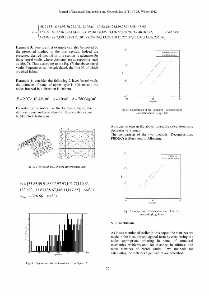
Example 4: consider the following 2 layer barrel vault, the diameter of panel of upper layer is 600 cm and the nodes interval in x direction is 100 cm.

3227 /780010/1007.2 mkgcmAmkNE By ordering the nodes like the following figure, the stiffness, mass and geometrical stiffness matrices can be like block tridiagonal.

Fig13. View of 2D and 3D from 2layers barrel vault

sradsrad

/66.326/]65.147,11.146,67.138,67.133,693.123

,63.110,71.102,93.97,02.86,91.59,85.55[

max


Fig 15. Comparison of pre - and post – decomposition calculation time. (Log. Plot)

As it can be seen in the above figure, the calculation time decreases very much. The comparison of the two methods (Decomposition, PBD&C) is illustrated in following:

Fig 16. Comparison of calculation time of the two methods. (Log. Plot)

5. Conclusions

As it was mentioned earlier in this paper, the matrices are made in the block three diagonal form by considering the nodes appropriate ordering in some of structural mechanics problems and, for instance, in stiffness and mass matrices of barrel vaults. Two methods for calculating the matrices eigen values are described. 50 100 150 200 250 300 350

0

1

2

3

4

5

6

7

eigenvalues

Num

ber of

eig

enva

lues

100

101

102

102

103

104

105

Time (Sec)

(Dof

)

Before Decomposition)After Decomposition

100

101

102

102

103

104

105

Time (Sec)

(Dof

)

First MethodSecond Method

L. Shahryari

28

1. The efficiency of algebraic graph theory in combinatorial optimization, especially in ordering and partitioning of graphs is well known. However, large structural models and their corresponding graphs require considerable computational time for evaluating their eigenvalues and eigenvectors. In this paper, using a new canonical form, a highly efficient method is presented for the eigensolution of some special structural(Barrel Vaults) and finite elementmodels which are often encountered in structural mechanics. 2. A mixed data/task parallel implementation of the block-tridiagonal divide and-conquer algorithm is presented. In this implementation processors are divided into subgrids, and each subgrid is assigned to a subproblem Because of the data distribution pattern, at the beginning of each merging operation, matrix subblocks must be redistributed. The communication overhead of data redistribution not only depends on interconnection of processors, but also on the topology of processor subgrids, all of which were considered. At the end the presented algorithm was compared with the MATLAB software from the point of view of calculation time and speed and the two mentioned methods were compared with each other. References [1] Agarwal, R. C., Gustavson, F. G. (1998). Algorithm and

architecture aspects of producing ESSLBLAS on Power2. In PowerPC and POWER2: Technical Aspects of the New IBM RS/6000, IBM ,Corporation, Armonk, NY, 167-176.

[2] Agarwal, R.C., Gustavson, F. G., And Zubair, and M. (1994). Improving performance of linear algebra algorithms for dense matrices using algorithmic prefetch. IBM J. Res. Devel, 38(3), 26-51.

[3] Bai, Y. (2005). High performance parallel approximate eigensolver for real symmetric matrices. Ph.D. Dissertation, University of Tennessee, Knoxville, TN.

[4] Bai, Y., Gansterer, W. N., And Ward, R. C.(2004). Block-tridiagonalization of effectively sparse symmetric matrices, ACM Transaction on Mathematics Software, 30, 326-352.

[5] Callaway, J. (1991). Quantum theory of the solid state, Academic Press, Boston, MA.

[6] Chakrabarti, S., Demmel, J., And Yelick, D.(1999). Modeling the benefits of mixed data and task parallelism. In proceeding of the 7th annual ACM symposium on parallel algorithms and architectures.Santa Barbara, CA, ACM Press, New York, NY, 74-83.

[7] Cuppen, J. J.M.(1998). A divide and conquer method for the symmetric tridiagonal eigenproblem, Communications in Numerical Methods in Engineering. 36, 177-195.

[8] Demmel, J., Mckenney, A.(1999). A test matrix generation suite. LAPACK working note 9. Courant Institute of Mathematical Sciences, New York, NY.

[9] Dewar, M. J. S., Thiel,W.(2004). Ground states of molecules, 38. The MNDO method. Approximations and parameters, Journal of American Chemical Society 99, 4899-4907.

[10] Kaveh, A., Sayarinejad, MA.(2004). Eigensolutions for factorable matrices of special patterns, Communications in Numerical Methods in Engineering. 20,133-146.

[11] Kaveh, A.(2004). Structural Mechanics Graph and matrix methods, Research

Studies Press (John Wiley), 3rd edition, Somerset, UK., [12] Kaveh, A., Sayarinejad, MA. (2004). Graph symmetry in

dynamic systems Computers and Structures. Nos 23-26(82), 2229-2240.

[13] Kaveh, A., Salimbahrami, B. (2004). Eigensolutions of symmetric frames using graph factorization. Communications in Numerical Methods in Engineering. 20, 889-910.

[14] Kaveh, A., Rahami, H. (2005). New canonical forms for analytical solution of problems in structural mechanics. Communications in Numerical Methods in Engineering. No. 9, 21499-513.

[15] Kaveh, A., Shahryari, L. (2008). Planar truss structures with multi symmetry. Proceedings of the Ninth International Conference on Computational Structures Technology, B.H.V. Topping and M. Papadrakakis. (Editors), Civil-Comp Press, Stirlingshire, Scotland.

[16] Yihua, B., (2005).. (2007). A parallel symmetric Block-Tridiagonal Divide-and-Conqur Algorithm, University of Tennessee,ACM Transation on Mathematica software , 4(33), 25-38.

[17] Kaveh, A. Shahryari, L. (2007) Eigenfrequencies of symmetric planar frames with semi-rigid joints using weighted graphs. Finite Elements in Analysis and Design. 43, 1135-1154.

[18] Kaveh, A., Shahryari, L. (2007). Buckling load of planar frames with semi-rigid joints by using weighted symmetric graphs. Computers and Structures. 85, 1704-1728.

[19] Kaveh, A. (2006). Optimal Structural Analysis, 2nd edn.Wiley, Somerset, UK.

[20] Kaveh, A., Sayarinejad, M.A. (2003). Eigensolutions for

matrices of special patterns. Communications in Numerical Methods in Engineering. 19, 125-136.

[21] Kaveh, A., Sayarinejad, M.A. (2005). Eigenvalues of factorable matrices with form IV symmetry. Communications in Numerical Methods in Engineering. 21, 269-278.

[22] Kaveh, A., Rahami, H. (2006). Block diagonalization of adjacency and Laplacian matrices for graph product. applications in structural mechanics. International Journal for Numerical Methods in Engineering. 68, 33-63.

[23] Robbe, M., Sadkane, M. (2005). Convergence analysis of the block householder block diagonalization algorithm. BIT Numerical Mathematics. 45, 181-195.

[24] Park, H. (1990). Efficient diagonalization of oversized matrices on a distributed-memory multiprocessor. Annals of Operation Research. 22, 253-269.

[25] Mathias, R., Stewart, G.W. (1993). A block QR algorithm and the singular value decomposition. Linear Algebra and its Application, 182, 91-100.

[26] Hasan, M.A., Hasan, J.A.K. (2002). Block eigenvalue decomposition using nth roots of identity matrix, 41st IEEE Conference, Decis.Control 2, 2119-2124.

[27] Gould, P. (1967). The geographical interpretation of eigenvalues. Trans. Inst. British Geographer. 42, 53-58 .

[28] Straffing, P.D. (1980). Linear algebra in geography eigenvectors of networks. Mathematics Magazine. 53, 269-276.

[29] Kaveh, A., Shahryari, L. (2010). Eigenfrequencies of symmetric planar trusses via weighted graph symmetry and new canonical forms, Engineering Computations, 3(27), 409-439.

[30] Grimes, R.G., Pierce, D.J., Simon, H.D. (1990). A new algorithm for finding a pseudo-peripheral node in a graph, SIAM Journal Analysis and Application, 11, 323-334.

free vibration analysis of repetitive structures using...

Documents