FORWARD INTEREST RATES AND VOLATILITY OF ZERO COUPON YIELD IN AFFINE MODELS

Medvedev Gennady

Faculty of Applied Mathematics and Computer Science Belarusian State University

4 F. Skorina ave. Minsk, 220050, Belarus Tel: + 0375 17 2095448 MedvedevGA@bsu.by

Abstract

The analysis of the forward rate curve for enough wide class of one factor affine models of the term structure that includes not only Vasiček’s Gaussian model and the square root model CIR but also models with any levels of the lower boundary of the short term (riskfree) interest rates is resulted. The multi-factor Gaussian model is discussed in details too. The special attention is given to the problem connected with the tendency for the term structure of long term forward rates to slope downwards.

For one-factor models with stochastic volatility the following results are de-rived: the probability that the forward rate curve slopes downwards for long term yield rates is found and is shown that this probability is influenced essen-tially not only by interest rate volatility but also by level of the lower boundary of short term rates and parameters of the risk premium; the expectations, vari-ances and covariances for the forward rates and the yield process volatility are calculated; the correlation between the forward rates and the yield process vola-tility is always positive and does not depend on term to maturity; its lower boundary is found; the average slope of the forward rate curves is negative for all terms to maturity.

For one factor models with deterministic volatility (Gaussian models) the probability that the forward rate curve slopes downwards for long term yield rates is found; this probability always increases as the term to maturity increases but has the upper boundary that is dependent on the interest rate volatility; in the mean the slope of the forward rate curve is too negative independent on term to maturity.

For multifactor Gaussian models the representation of state variable process in the explicit form is derived and its covariance matrix is found; the probability that the forward rate curve slopes downwards is found also.

Keywords: forward rate curve, volatility of zero coupon yield, affine model,

Vasiček’s Gaussian model, square root model CIR, term structure of long-term forward rates.

Introduction

One of classical problems of financial economics is the analysis of behav-

iour of the yield on default free bonds depending on their maturities. At the cer-tain assumptions it is possible to use mathematical model of available yield curve to extrapolate it to obtain the future values of yield rates. The forward rates can be obtained on the basis of knowledge of time structure of discount bonds (see details in Hull (1993)).

The forward rate term structure was investigated in a number of references from which we shall mention only a few. D. Heath, R. Jarrow, and A. Morton (1992) have developed the methodology for obtaining of stochastic processes of subsequent movements of forward rate curve. Brown and Schaefer (1994) have derived a forward rate curve for affine models of term structure. Kortanek and Medvedev (2001) have offered a minimax way of modelling forward curve on the basis of the observation of yield. Medvedev (2003) has presented the com-parative analysis of yield curves and forward rate curves.

At the same time the area of term structure for long-term forward rates was not subject to detailed research as for short-term interest rates. Brown and Schaefer (2000) have discovered that the new information about the yield term structure can be received from the analysis of the long-term end of the forward rate curve. They have noted that the empirical data show that the forward rate curve for long term maturity is usually sloped downwards. Discussion of two factor Gaussian affine model of term structure at the certain assumptions has al-lowed to draw an inference that the slope of the forward rate curve on the long-term end always should be negative and this effect is connected to properties volatility of long term zero coupon yield. Moreover that is possible to predict volatility of long-term yield by observation a slope of the forward rate curves. This problem was empirically investigated Christiansen (2001), which provides cautious support to results of Brown and Schaefer (2000).

In the present paper the analysis of the forward rate curve is made for wider class of affine one factor models of the term structure including not only Va-siček’s Gaussian model (1977) and the square root model CIR (1985) but also the models generated by the short term (riskfree) interest rates with the various levels of the lower boundary [see Ilieva (2000, 2001) or Medvedev (2003)]. The multifactor Gaussian model is discussed in details too.

Properties of forward rate curves for affine models

of term structure

The affine models of term structure occur when the short term (riskless) in-terest rate r(t) follows the stochastic process described by the stochastic differential equation

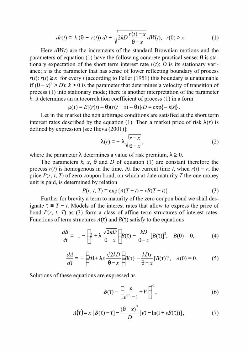
dr(t) = k (θ − r(t)) dt + xxtrkD

−θ−)(2 dW(t), r(0) > х. (1)

Here dW(t) are the increments of the standard Brownian motions and the parameters of equation (1) have the following concrete practical sense: θ is sta-tionary expectation of the short term interest rate r(t); D is its stationary vari-ance; х is the parameter that has sense of lower reflecting boundary of process r(t): r(t) ≥ х for every t (according to Feller (1951) this boundary is unattainable if (θ – x)2 > D); k > 0 is the parameter that determines a velocity of transition of process (1) into stationary mode; there is another interpretation of the parameter k: it determines an autocorrelation coefficient of process (1) in a form

ρ(τ) = E[(r(t) – θ)(r(t + s) – θ)]/D = exp{ – k|s|} . Let in the market the non arbitrage conditions are satisfied at the short term

interest rates described by the equation (1). Then a market price of risk λ(r) is defined by expression [see Ilieva (2001)]:

λ(r) = − xxr

−θ−λ , (2)

where the parameter λ determines a value of risk premium, λ ≥ 0. The parameters k, x, θ and D of equation (1) are constant therefore the

process r(t) is homogenous in the time. At the current time t, when r(t) = r, the price P(r, t, Т) of zero coupon bond, on which at date maturity Т the one money unit is paid, is determined by relation

P(r, t, Т) = exp{A(Т − t) − rВ(Т − t)}. (3) Further for brevity a term to maturity of the zero coupon bond we shall des-

ignate τ ≡ Т − t. Models of the interest rates that allow to express the price of bond P(r, t, Т) as (3) form a class of affine term structures of interest rates. Functions of term structures A(τ) and В(τ) satisfy to the equations

=τd

dB 1 −

−θ

λ+x

kDk 2 B(τ) − x

kD−θ

[B(τ)]2, B(0) = 0, (4)

=τd

dA −

−θ

λ+θx

kDxk 2 B(τ) x

kDx−θ

− [B(τ)]2, A(0) = 0. (5)

Solutions of these equations are expressed as

В(τ) = 1

1

−

ετ

+

−ε V

e, (6)

( ) ])([ τ−τ=τ BxA ))](1ln([)( 2τ+−τ−θ− vBv

Dx , (7)

where it is designated for brevity

,0422

>≥−θ

+

−θ

λ+=ε kx

kDx

kDk

(8)

0221 ≥

−θ

λ−−ε=x

kDkv , .0221 >≥

−θ

λ++ε= kx

kDkV

Note that v + V = ε, vV = kD/(θ − x). Properties of functions of affine term structure A(τ) and В(τ) that are de-

termined by formulae (6) – (7) are in detail investigated in Ilieva (2000). The forward rate f(t, Т, T′) determines the bond yield between dates Т and

T′ such that t < Т < T′ on the base of information about yield that is available at time t:

f(t, Т, T′) =

′−′ ),,(),,(ln1

TrtPTrtP

TT =

τ−τ′τ+τ′−τ−τ′ )()()]()([ AABBr , (9)

where τ′ = Т′ − t. As Т′ → Т, i.e. τ′ → τ, the forward rate (9) turn into the so-called instantaneous forward rate

f(t, Т) = f(τ) = T

TrtP∂

∂− ),,(ln = ττ−

ττ

ddA

ddBr )()( , (10)

which is used more often as it is connected by enough simple relations with bond yield to maturity у(t, Т) = у(τ)

f(t, Т) = f(τ) = T

TtytT∂

−∂ )],()[( = τττ+τ

ddyy )()( . (11)

Therefore more often a word-combination «the forward rate» means the instan-taneous forward rate.

For the term structure models of the affine yield class Brown and Schaefer (1994) have offered to consider a forward rate curve of f(τ) as the complicated function that depends on term to maturity τ only through the function of affine structure В(τ), i.e. f(τ) ≡ F(В(τ)). First, it is convenient because an interval of possible values of function В(τ) is finite according to (6). In this connection the properties of functions F(В) can be illustrated visually by plots on the whole of interval (0, ∞) possible values of terms to maturity τ. Second, as it was men-tioned in CIR (1979) it is possible to consider the function В(τ) as a measure of a duration because by analogy with the standard duration of the bond price with respect to the interest rates (in this case with respect to short term rates) this function is determined by the formula B(τ) = − [∂P/∂r]/P.

It is obtained from expression (4), (5) and (10) that

f(τ) ≡ F(В(τ)) = r +

−θ−λ−−θ

xxrkDrk 2)( B(τ) − kD

xxr

−θ− B(τ)2 ≡

≡ r + [k(θ − x) − (V − v)(r − x)] B(τ) − vV(r − x) B(τ)2. (12)

The general properties of the forward rate curves f(τ) are presented in Med-vedev (2003). Here we shall consider in more detail behavior of a forward curve for the long terms to maturity τ.

From expression (10) it follows that

ττ

ddf )( = 2

2

2

2 )()(τ

τ−τ

τd

dAdBdr

From the relations (4) − (7) it is possible to find that

)),(1))((1()( τ−τ+=ττ VBvB

ddB ,)())(2()(

2

2

τττ+−−=

ττ

ddBvVBvV

dBd

.)())(1))((1)(()(2

2

2

2

ττ+τ−τ+−θ−=

ττ

dBdxVBvBxk

dAd

Therefore

ττ

ddf )( = +

ττ− 2

2 )()(dBdxr =τ−τ+−θ ))(1))((1)(( VBvBxk

= [k(θ − x) − [v + V − 2v(1 − VB(τ))](r − x)] )).(1))((1( τ−τ+ VBvB (13)

From (6) it follows that as τ → ∞ the function B(τ) → V −1. Hence for f(τ) and ττ ddf )( there are the limit relations as τ → ∞

f(τ) → f(∞) ≡ ,1 xVk

Vk

−+θ

ττ

ddf )( → 0. (14)

It means that if the terms to maturity increase then the forward rates tend to a constant, which takes values from an interval [х, θ] since by definition

.10 ≤< Vk It is interesting to explain under what conditions the forward rate curve

slopes downwards (i.e. has negative derivative) at long term to maturity. As it follows from representation (13) the derivative ττ ddf )( is expressed in the form of product of three factors, two of which (the second and the third) are not negative by the definition. Therefore the forward rate curve slopes downwards if the following inequality is valid

k(θ − x) − [v + V − 2v(1 − VB(τ))](r − x) < 0,

that it is more convenient to write

.))(1(2 τ−−+

>−θ−

VBvVvk

xxr (15)

Because the function B(τ) increases monotonously from the value B(0) = 0 at τ = 0 up to the value B(∞) = V −1 at τ = ∞, hence the right part of the inequal-ity (15) is monotonously decreasing function τ from value k/(V − v) at τ = 0 up to k/(V + v) at τ = ∞.

Thus the forward rate curve slopes downwards for any τ if

,vV

kxxr

−>

−θ− (16)

and can have the negative slope for the some enough long maturities τ > τ0(r) if

.vV

kxxr

vVk

+>

−θ−>

− (17)

Here it is designated by τ0(r) such value τ, at which the inequality (15) turns into equality.

Using formulae (8) it is possible to write inequalities (15) – (17) in the ex-plicit form through parameters of model (1).

Let's remind that by definition r = r(t) is a value of process of the short term rate at time t. Hence this value can be considered as random variable. It is known also [Ilieva (2000)] that process r(t) that is determined by the equation (1) under the conditions accepted above has the shifted gamma distribution with the following parameters: parameter of shift х, parameter of scale D/(θ − x) and parameter of the form (θ − x)2/D.

The probability density function of this random variable r is

,))((exp)(

)()(

2

1)()( 22

−−θ−

−θΓ

−

−θ

=

−−θ−θ

Dxrx

Dx

xrD

x

rgDx

Dx

r > х. (18)

Let's remind that the inequality (θ – x)2 > D takes place according to Feller’s condition for unattainability of the lower boundary of the short term rate process r(t) accepted above. Therefore the parameter of the form (θ − x)2/D > 1.

It is more convenient to deal not with the random variable r but with its af-fine transformation z = (r − x)/(θ − x). The random variable z has the ordinary gamma distribution with parameter of the form (θ − x)2/D and parameter of scale

D/(θ − x)2. Let's designate the gamma distribution function with parameter of the form α and parameter of scale β through G(r | α, β). Then the probability PSD, that it is existing τ0(r) < ∞ such that for enough long terms to maturity τ > τ0(r) the forward interest rates will slope downwards, is equal to probability of ful-fillment of inequalities (16) or (17), i.e.

PSD = 1 – .)(

,)(2

2

−θ−θ

+ xD

Dx

VvkG (19)

Thus, PSD depends not only from parameters k, x, θ and D of process (1) but also on a parameter of a market price of risk λ through values v and V (see the formula (8)). Figure 1 presents PSD as function of arguments х and λ for values of parameters k ==== 0,2339, θ ==== 0,0808 and D ==== 0,00126 corresponding to the empirical estimations received in CKLS (1992) at analysis of the annualized one-month U.S. Treasury bill yield from June 1964 to December 1989 (306 observations). Figure 2 presents PSD as function arguments х and D for values of parameters k ==== 0,892, θ ==== 0,0905 and λ ==== 0,0789 according to the empirical estimations received in Aït-Sahalia (1996) at analysis the 7-day Eurodollar

timations received in Aït-Sahalia (1996) at analysis the 7-day Eurodollar deposit

Fig. 1. Probability PSD that for enough long maturities the forward rate curve will slope downwards as function of the lower boundary х of process of the short term rate at various

values of parameter λ market price of risk.

0,0

0,2

0,4

0,6

0,8

1,0

0,00 0,02 0,04 0,06 0,08x

PSD

λ = 0 λ = 0,05 λ = 0,1 λ = 0,2λ = 0,3 λ = 0,5 λ = 0,75 λ = 1,0

Fig. 2. Probability PSD that for enough long terms to maturity the forward rate curve will slope downwards as function of the lower boundary х of process of the short term rate at vari-

ous values of stationary variance D of the short term interest rate. spot rate, daily from 1 Jun 1973 to 25 Feb 1995 (5505 observations). Note that according to the Feller’s condition of unattainability of lower boundary for set of parameters given on figure 2 the variance D cannot be more 0,008.

From these figures it follows that probability PSD is more sensitive to pa-rameter λ market price of risk than to stationary variance D of the short-term in-terest rate, i.e. to volatility of yield process that is directly proportional .D

The probability PSD that the forward rate curve slopes downwards at some maturity τ is determined as the probability that the inequality (15) is held. Tables 1 and 2 present the estimates of parameters that influence on this probability for some real data. The parameter v for these real data is very close to zero and this fact practically exclude a dependence on time to maturity τ for probability at these data. The values of probabilities PSD are shown in the Table 2. They are not exceeded 0,5.

In conclusion of this section we note that from representation (6) it follows that for the long terms to maturities VB(τ) ≈ 1 − ε е−ετ/V. Therefore for the long maturities τ the formula (13) for a derivative of forward rate curve can be pre-sented as

ετ−

ε−ε−−θ=

ττ e

Vxrxk

drdf 2

)]()([)|( + о(е−ετ). (20)

This implies that on the long-term end of term structure the derivative ττ drdf )|( on absolute value exponentially decreases.

0,0

0,2

0,4

0,6

0,8

1,0

0,00 0,03 0,06 0,09x

PSD

D = 0,0005; D = 0,001; D = 0,002; D = 0,003;D = 0,004; D = 0,006; D = 0,008;

Forward rates and yield volatility

The term structure of forward rates f(τ) ≡ f(τ|r) is defined by equation (12).

In this expression as already it has above been told the only variable can be con-sidered as random. It is r – a value of riskfree interest rate at present time t. Ac-cording to (3) by the same reason the yield to maturity is also a random variable and its volatility σу(τ|r) differs from volatility of short term rates only by multi-plier B(τ)/τ, i.e.

σу(τ|r) = .2)(xxrkDB

−θ−

ττ (21)

The random variable r has the probability density function that is deter-mined by expression (18). Therefore it is possible to calculate the moments f(τ|r) and σу(τ|r) that results in to formulae

E[f(τ|r)] = θ + [k − (V − v) − vVB(τ)](θ − x)B(τ) =

= θ − [λ 2 + kD B(τ)] kD B(τ). (22) Var[f(τ|r)] = [(1 − VB(τ))(1 + vB(τ))]2D. (23)

E[σу(τ|r)] = .)(2 QBkDττ (24)

Varσу(τ|r)] = ).1()(2 22

QBkD −

ττ (25)

Here for brevity the designation is used

Q ≡ ,)(21)( 22

−θΓ−θ

+−θΓ

Dx

Dx

Dx (26)

where by symbol Г (.) the gamma function is designated. It follows from the properties of gamma functions that the function Q(и) = ,)]([)21( 2/1 uuu Γ+Γ that is set by formula (26), is determined only for positive values of argument and monotonously increases. Furthermore Q(и) 24/11 u+ → 1 as и → ∞. Be-cause it is assumed that the Feller’s condition for unattainability of the lower boundary by the riskfree rate process r(t) is fulfilled then this is equivalent to inequality и = (θ − x)2/D > 1. The calculation show that for и > 1 there is ful-filled Q(и) > 0,8, i.e. .3/4)]([1)( 2 >− uQuQ

Covariance of the forward rate f(τ|r) and volatility σу(τ|r) is expressed by the formula

Cov[f(τ|r), σу(τ|r)] = [(1 − VB(τ))(1 + vB(τ))] .2

)(2x

DQBkD−θτ

τ (27)

From this by expressions (23) and (25) it is easy to calculate the correlation coefficient of forward rate f(τ|r) and volatility σу(τ|r) in the form

ρ = .0)(3

21)(2

12

22 >

−θ>−

−θ xDQ

xDQ (28)

So the correlation of the forward rate f(τ|r) and the volatility yield process σу(τ|r) is always positive and their correlation coefficient can not be less than (2/3)D/(θ − x)2.

In addition it is interesting to note that in spite of the fact that expectations and variances of the forward rate f(τ|r) and the volatility yield process σy(τ|r) depend on the term to maturity τ the correlation between these functions does not depend on τ and is the same for all maturities and monotonously decreases with growth of value и = (θ − x)2/D. For example, as u increases from 1 up to 20 the correlation coefficient ρ decreases from 0,9565 up to 0,2229.

For affine Gaussian model of term structure, i.e. Vasiček’s model, the lower boundary of the riskfree rates х = − ∞. Therefore for this model u → ∞ and then Q(и) → 1. Estimate the correlation coefficient for this case. At great values u for asymptotic representations of gamma function it is possible to use the Stirling’s formula

Γ(u) = .12112 21

++π −−

uo

ueu uu

Use of this extension in the formula (28) results in expression for great val-ues of argument u = (θ − x)2/D:

ρ = .)()(32

31 22

−θ

+−θ

−−θ x

Dox

Dx

D

Thus, as х → − ∞ the correlation coefficient ρ → 0. It is a natural result (in Vasiček’s model the volatility is deterministic) as in Gaussian models of term structure the correlation of the forward rate f(τ|r) and the yield process volatility σy(τ|r) is absent.

For model of the term structure generated by riskfree rate process r(t) «with a square root», i.e. the CIR models, the lower boundary of riskfree rates х = 0. In table 1 the empirical data are given for the CIR model parameters that is esti-mated by different authors and corresponding values of the correlation coeffi-cient ρ are given too. In this table by the symbol σ is designated the volatility parameter of the short term interest rate for standard representation of CIR model for process r(t)

dr(t) = k (θ − r(t)) dt + σ )(tr dW(t).

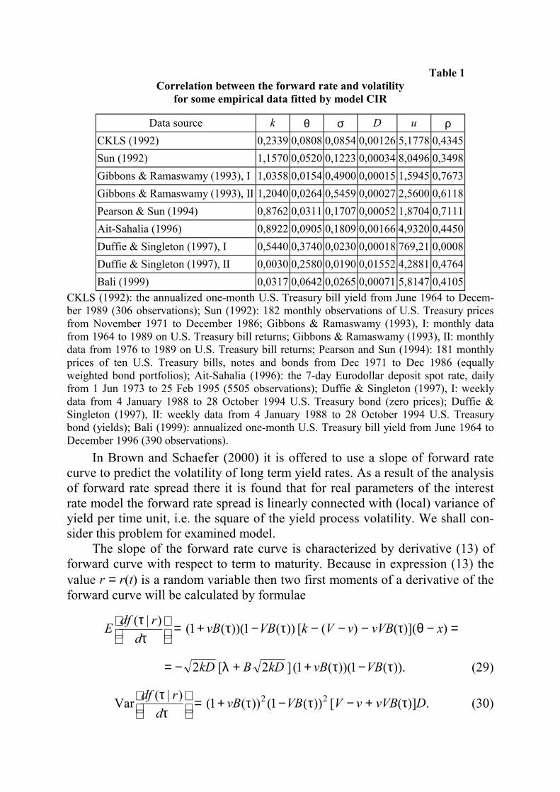
Table 1 Correlation between the forward rate and volatility

for some empirical data fitted by model CIR

Data source k θ σ D и ρ CKLS (1992) 0,2339 0,0808 0,0854 0,00126 5,1778 0,4345 Sun (1992) 1,1570 0,0520 0,1223 0,00034 8,0496 0,3498 Gibbons & Ramaswamy (1993), I 1,0358 0,0154 0,4900 0,00015 1,5945 0,7673 Gibbons & Ramaswamy (1993), II 1,2040 0,0264 0,5459 0,00027 2,5600 0,6118 Pearson & Sun (1994) 0,8762 0,0311 0,1707 0,00052 1,8704 0,7111 Ait-Sahalia (1996) 0,8922 0,0905 0,1809 0,00166 4,9320 0,4450 Duffie & Singleton (1997), I 0,5440 0,3740 0,0230 0,00018 769,21 0,0008 Duffie & Singleton (1997), II 0,0030 0,2580 0,0190 0,01552 4,2881 0,4764 Bali (1999) 0,0317 0,0642 0,0265 0,00071 5,8147 0,4105

CKLS (1992): the annualized one-month U.S. Treasury bill yield from June 1964 to Decem-ber 1989 (306 observations); Sun (1992): 182 monthly observations of U.S. Treasury prices from November 1971 to December 1986; Gibbons & Ramaswamy (1993), I: monthly data from 1964 to 1989 on U.S. Treasury bill returns; Gibbons & Ramaswamy (1993), II: monthly data from 1976 to 1989 on U.S. Treasury bill returns; Pearson and Sun (1994): 181 monthly prices of ten U.S. Treasury bills, notes and bonds from Dec 1971 to Dec 1986 (equally weighted bond portfolios); Ait-Sahalia (1996): the 7-day Eurodollar deposit spot rate, daily from 1 Jun 1973 to 25 Feb 1995 (5505 observations); Duffie & Singleton (1997), I: weekly data from 4 January 1988 to 28 October 1994 U.S. Treasury bond (zero prices); Duffie & Singleton (1997), II: weekly data from 4 January 1988 to 28 October 1994 U.S. Treasury bond (yields); Bali (1999): annualized one-month U.S. Treasury bill yield from June 1964 to December 1996 (390 observations).

In Brown and Schaefer (2000) it is offered to use a slope of forward rate curve to predict the volatility of long term yield rates. As a result of the analysis of forward rate spread there it is found that for real parameters of the interest rate model the forward rate spread is linearly connected with (local) variance of yield per time unit, i.e. the square of the yield process volatility. We shall con-sider this problem for examined model.

The slope of the forward rate curve is characterized by derivative (13) of forward curve with respect to term to maturity. Because in expression (13) the value r = r(t) is a random variable then two first moments of a derivative of the forward curve will be calculated by formulae

ττ

drdfE )|( = ))(1))((1( τ−τ+ VBvB [k − (V − v) − vVB(τ)](θ − x) =

= − kD2 [λ + В kD2 ] )).(1))((1( τ−τ+ VBvB (29)

ττ

drdf )|(Var = 22 ))(1())(1( τ−τ+ VBvB [V − v + vVB(τ)]D. (30)

Two first moments of 2yσ (τ|r) =

xxrkDB

−θ−

ττ 2)( 2

, i.e. the (local) variance

of yield per the time unit, are expressed in the form

Е[ 2yσ (τ|r)] = .2)( 2

kDB

ττ Var[ 2

yσ (τ|r)] = .)(

)2()(2

24

xDkDB−θ

ττ (31)

The covariance of the forward curve derivative and the yield variance is de-termined by the formula

Cov

σ

τ2, yd

df = − ))(1))((1( τ−τ+ VBvB [V − v + vVB(τ)] .2)( 22

xkDB−θ

ττ

From here it follows that the correlation coefficient of the forward curve derivative and the yield variance for all maturities τ is equal to the minus unit:

ρ = .1][Var][Var

],[Cov2

2

−=στ

στ

y

y

ddf

ddf (32)

It means that these characteristics are linearly connected between them-selves. Actually this fact is easy to set. If from formulae (13) and (21) to express value (r − х) and to equate the obtained results then we obtain the following re-lation that is valid with probability 1 for any τ:

2yσ (τ|r) =

2)(

ττB .

))]((2))[(1))((1(2)])|(()))((1))((1([xvVBvVVBvB

kDdrdfxVBvBk−θτ+−τ−τ+ττ−−θτ−τ+ (33)

Thus on the basis of the above analysis it is possible to draw the following conclusions:

− the expectation of the derivative of forward rate curve with respect to term to maturity (29) is negative. It means, that in mean the slope of forward rate curve is negative for any terms to maturity τ;

− the derivative of the forward rate curve with probability unit is con-nected with (local) variance of yield by affine relation (33) for any terms to ma-turity τ;

− the correlation coefficient of the forward curve derivative and variance of yield (32) for all terms to maturity τ is equal to the minus unit at any values of the parameters having real economic sense.

Generally speaking, the formula (33) can be considered as a basis for de-termination of the local variance of yield 2

yσ (τ|r) by the forward curve deriva-tive ττ drdf )|( if this derivative can be estimated. Let's consider such opportu-nity. For convenience of reasoning it is convenient to present the formula (33) as

2yσ (τ|r) = ,)|()()()(

τττζ−−θτξ

drdfxk (34)

where

ξ(τ) ≡ 2)(

ττB ,

))]((2[2

xvVBvVkD

−θτ+− ζ(τ) ≡

))(1))((1(1

τ−τ+ VBvB.

Note that the difference in the right part (34) is always positive as from rep-resentation (13) it follows that

.0))(1))((1(

))]((2[)|()()( >τ−τ+−τ+−=

τττζ−−θ

VBvBxrvVBvV

drdfxk

At small τ function B(τ) has representation B(τ) = τ + О(τ2). Therefore for small τ the formula (33) can be written as

2yσ (τ|r) ≈

kDxkkD

2)(2

λ+−θ.)|()(

ττ−−θ

drdfxk (35)

At long τ there is representation VB(τ) ≈ 1 − ε е−ετ/V and the formula (34) can be approximately written as:

2yσ (τ|r) ≈ .)|()(2

2

2

2

ττ

ε−−θ

τε

ετ

drdfeVxk

Vv (36)

Thus as it follows from representation (20) at long τ the derivative of for-ward rate curve exponentially decreases as τ increases, and the coefficient be-fore a derivative in the formula (36) exponentially increases. It means that even small errors in estimation of the derivative of forward rate curve can be in-creased "exponentially" and the calculation of 2

yσ (τ|r) by formula (34) can have the big errors.

For the real empirical data that presented in Table 1 the values of parame-ters are such that V ≈ ε, and parameter v is very small. In that case the formula (36) can be rewritten as

2yσ (τ|r) ≈ ,)|(

2

ττ−ψ

τϕ ετ

drdfe (37)

where ϕ = 2v/ε2 and ψ = k(θ − х). In Table 2 values of these coefficients are pre-sented. We shall remind that empirical data of Tables 1 concern to approxima-tion of the real data in a case when the short term rates are generated by the CIR model, i.e. х = 0.

Table 2 Probability PSD and coefficients ϕϕϕϕ and ψψψψ of formula (37)

for some empirical data fitting by the CIR model

Data source ε v V PSD ϕ ψ CKLS (1992) 0,23390 1,261E-06 0,23390 0,442 4,609E-05 0,0189 Sun (1992) 1,15700 3,363E-07 1,15700 0,453 5,024E-07 0,0602

Gibbons & Ramaswamy (1993), I 1,03620 1,487E-07 1,03620 0,395 2,769E-07 0,0160 Gibbons & Ramaswamy (1993), II 1,20451 2,721E-07 1,20451 0,417 3,751E-07 0,0318

Pearson & Sun (1994) 0,87639 5,17E-07 0,87633 0,403 1,347E-06 0,0273 Ait-Sahalia (1996) 0,89219 1,660E-06 0,89219 0,440 4,172E-06 0,0807

Duffie & Singleton (1997), I 0,54400 1,818E-07 0,54400 0,500 1,228E-06 0,2035 Duffie & Singleton (1997), II 0,00303 1,544E-05 0,00302 0,445 3,36133 0,0008

Bali (1999) 0,03170 7,088E-07 0,03170 0,445 1,411E-03 0,0020

The analysis shows that if instead of derivative of the forward rate curve to use the forward rate spread then results will be very similar insignificantly dif-fering in details. Really let τ2 = τ + δ, τ1 = τ − δ. We shall introduce designations ∆B(τ, δ) ≡ B(τ2) − B(τ1), ∇ B(τ, δ) ≡ B(τ2) + B(τ1). Then the forward rate spread with the help (12) it is possible to express as

∆f(τ, δ) ≡ f(τ2|r) − f(τ1|r) =

=

−θ−λ−−θ

xxrkDrk 2)( − kD

δτ∇−θ− ),(B

xxr ∆В(τ, δ). (38)

Now using that 2yσ (τ|r) =

xxrkDB

−θ−

ττ 2)( 2

it is possible to write the rela-

tion which with probability unit connects the spread ∆f(τ, δ) with the (local) variance of the yield per time unit 2

yσ (τ):

∆f(τ, δ) = )( xk −θ ∆В(τ, δ) −

− )(2

),()(

)],(2)([ 22

τσδτ∆

τ

τδτ∇+λ+−θ ykDB

BBkDkDxk . (39)

Thus between the spread ∆f(τ, δ) and the variance of the yield per time unit 2yσ (τ) there is nondegenerated linear connection and hence their correlation co-

efficient is equal to minus unit as well as in (32). Again as well as in (34) we express from the relation (39) the local variance of yield per time unit 2

yσ (τ) through the spread ∆f (τ, δ) and estimate the coefficients in a formula obtained for the long terms to maturity.

2yσ (τ) =

δτ∆δτ∆−−θ

ττ

δτ∇+λ+−θ ),(),()()(

),(2)(2 2

BfxkB

BkDkDxkkD . (40)

Let's name the term to maturity τ as long if it is possible to neglect the terms of the order O(е−ετ) in comparison with unit. In this case as well as in ex-pression (36) it is possible the representation VB(τ) ≈ 1 − ε е−ετ/V. Therefore it is possible to write that ∇ B(τ, δ) ≈ 2/V and also ∆B(τ, δ) ≈ εе−ετd(ε, δ)/V 2 where d(ε, δ) = (еεδ − е−εδ). Then for representation 2

yσ (τ) it is possible to use the for-mula similar (34) again.

2yσ (τ) ≈

δεδτ∆

ε−−θ

τε

ετ

),(),()(2 2

2 dfeVxk

Vv ≡ ξ(τ)[k(θ − x) − ζ(τ)∆f(τ, δ)] (41)

or

∆f(τ, δ) ≈ .)(2

)(),( 22

τσετ−−θδεε ετ−

yvVxke

Vd (42)

Hence at long terms to maturity the order of smallness of coefficients ξ(τ) and ζ(τ) for any finite values τ2 − τ1 = 2δ remains the same, as well as in a case when instead of spread the derivative of the forward curve is used. Therefore all remarks concerning the error of calculations of the local variance of yield per time unit 2

yσ (τ) through a derivative of forward rate curve (see formula (36)) are valid for spread ∆f (τ, δ) too. At last at small δ we have that d(ε, δ) ≈ 2δε. There-fore as δ → 0 formula (40) will turn to the formula (36).

In conclusion note that the problem of the prediction of the volatility of long term yield through the slope of the forward rate curve was investigated by Brown and Schaefer (2000) for two factor affine Gaussian models of term struc-ture. In particular they deduced the relation ∆f (τ1, τ2) ≈ − 0,5 )( 2

122

2 τ−τσy . This relation has been obtained in the assumption that value k (θ − х) (in our designa-tions) is enough small and the first term in brackets in formula (41) could be ne-glected. In our case not Gaussian models if to neglect this factor then the follow-ing formula is obtained

∆f(τ1, τ2) ≡ ∆f(τ, δ) ≈ ).()(2

),( 22 τσετδε− ετ−ye

vVd (43)

Difference will be in that the coefficient of proportionality between the spread ∆f(τ1, τ2) and the local variance 2

yσ (τ) is equal to not τ2 but (ετ)2е−ετ, i.e. appears still an exponential reduction of the coefficient of proportionality.

Consider an error of such approximation. The forward rate spread is deter-mined by equation (39) as the sum of two terms first of which is deterministic and the second term is stochastic. The approximation (43) is reduced to that the

first term is rejected and as the forward rate spread is accepted the second term. Practically it means that approximation (43) simply changes the expectation of the forward rate spread by value of the first term in (39) at long rates. The ex-pectation of the forward rate spread according to formulae (31) and (39) is

Е[∆f(τ, δ)] = )( xk −θ ∆В(τ, δ) −

− ),())]()((2)([ 21 δτ∆τ+τ+λ+−θ BBBkDkDxk . At approximation (43) this expectation is changed by value of the first term.

For the zero risk premium (λ = 0) expression for the expectation can be written in the form Е[∆f(τ, δ)] = k(θ − x)∆В(τ, δ) − k(θ − x)[1 + vV(B(τ1) + B(τ2))/k]∆В(τ, δ). Hence it follows that the relation of the first term to the second on absolute

value is equal

χ = ),(]/))()((1)[(

),()(

21 δτ∆τ+τ+−θδτ∆−θ

BkBBvVxkBxk =

kBBvV /))()((11

21 τ+τ+.

From properties of function В(τ) we have that it monotonously increases from 0 at τ = 0 up to 1/V at τ = ∞. Therefore the relation χ monotonously de-creases from 1 at τ = 0 up to value [1/(1 +2v/k)] at τ = ∞. By definition v < k, therefore for any terms to maturity τ the inequality is realized χ > 1/3. As it is seen from Table 2 for real cases the parameter v is close to zero. It means that in real models χ ≈ 1. Therefore approximation (43) can be considered satisfactory only when the first term in (39) close to zero because in this case the change of Е[∆f(τ, δ)] is not essential.

Gaussian model

It has been told above that Brown and Schaefer (2000) have considered a two-factor time homogeneous affine Gaussian model of the term structure. In Christiansen (2001) the problem of adequacy of the Gaussian model of term structure was examined in the area of long-term maturities. The Gaussian mod-els are differed from considered above by assumption that the volatility of the riskfree interest rates is deterministic and the correlation relation (32) is not valid for Gaussian model. Therefore there is a sense to consider separately a problem of connection between properties of the forward rate curves and the yield volatilities in this case.

The affine Gaussian model is obtained when the riskfree interest rates are generated by the Vasiček model that is a special case of model (1) at х → − ∞, i.e. the lower boundary of the interest rate tends to the minus infinity. So ana-lytical results for Gaussian model can be received by corresponding limiting transition. In particular from formulae (6) – (8) it follows that as х → − ∞ the key parameters take values: v = 0, V = ε = k, and the function of term structure B(τ) = (1 − е−kτ)/k.

The local variance of yield process per time unit (the square of yield volatil-ity) is deterministic and is expressed by the formula 2

yσ (τ) = ( ) .)( 2 DB ττ The forward rates curve has form

f(τ|r) = r + ]2)([ kDrk λ−−θ B(τ) − kDB(τ)2 =

= r + ,2/)()()()( 22 τστ−τλτσ−τ−θ yyBrk its derivative with respect to τ that determines a slope is

ττ

ddf )( = .]2)22()([ τ−τ−++λ−−θ kk eDeDkDrk

When τ → ∞ we have B(τ) → 1/k and

f(τ|r) → f(∞) = ),2(1 kDDk

λ+−θ ττ

ddf )( → 0.

The riskfree rate process r(t) dr(t) = k (θ − r(t)) dt + kD2 dW(t)

is the Gaussian process and has a stationary normal distribution of probabilities with expectation θ and variance D.

Therefore probability PSD(τ) of that the forward rate curve at maturity term τ slopes downwards is equal

PSD(τ) = Pr )}(2/2{ τ−λ−θ> BDkr = Φ( )),(2/2 τ+λ BDk (44) where Ф is the standard normal distribution function. Because B(τ) is monoto-nously increasing function then PSD(τ) increases with τ too, PSD(τ) takes the value Φ( )/2 kλ at τ = 0 and reaches the maximal value Φ( )/2/2 kDk +λ at τ = ∞. Note that this maximum depends essentially on parameter k and in-creases as this parameter decreases.

In Table 3 the estimations of parameters of the Vasiček models are submit-ted that are obtained by different authors for the corresponding real data and the maximal values of probability PSD in the assumption that λ = 0 (in this case minimal PSD = 0,5 at τ = 0 for all variants). In this table a symbol σ is the vola-tility parameter of the short term interest rate in standard representation of Va-siček model for process r(t), i.e. kD2=σ .

Table 3 Estimations of Vasiček model parameters

Data source k θ σ D max PSD CKLS (1992) 0,1779 0,0866 0,0200 0,001124 0,6469 Ait-Sahalia (1996) 0,8584 0,0891 0,0467 0,001270 0,5331 Bali (1999) 0,0436 0,0642 0,0077 0,000680 0,8842 Ait-Sahalia (1999) 0,2610 0,0717 0,0224 0,000961 0,5939

CKLS (1992): the annualized one-month U.S. Treasury bill yield from June 1964 to Decem-ber 1989 (306 observations). Ait-Sahalia (1996): the 7-day Eurodollar deposit spot rate, daily from 1 Jun 1973 to 25 Feb 1995 (5505 observations). Bali (1999): annualized one-month U.S. Treasury bill yield from June 1964 to December 1996 (390 observations). Ait-Sahalia (1999): the Federal Reserve System funds data monthly from January 1963 to December 1998.

Figure 3 shows the plots of probability PSD as the function of maturity term τ that are calculated for data of Tables 3 in the assumption that λ = 0.

The expectation of forward rates E[f(τ|r)] = θ − λ kD2 B(τ) − kDB(τ)2.

The variance of forward rates Var[f(τ|r)] = D е− 2kτ.

Fig. 3. Probability PSD that the forward rate curve slopes downwards as a function of maturity term τ for data of Table 3.

As the variance of the yield to maturity for the affine term structure models is equal )(2 τyD = B(τ)2D/τ2 then the relation between expectation of forward rates and the yield variance be presented as follows

E[f(τ|r)] = θ − λ k2 τ )(τyD − k τ2 )(2 τyD .

The average slope of the forward rate curves (expectation of a derivative) and variance of the derivative

ττ

ddfE )( = ,0)](22[ <τ+λ− τ−kekDBkD

ττ

drdf )|(Var = k2D е− 2kτ.

The spread of forward rates for τ2 = τ + δ, τ1 = τ − δ:

0,50

0,55

0,60

0,65

0,70

0,75

0,0 5,0 10,0 15,0τ

PSD

CKLS A-S_96 Bali A-S_99

∆f(τ, δ) ≡ f(τ2|r) − f(τ1|r) = kDrk 2)([ λ−−θ − kD )],( δτ∇ B ∆В(τ, δ).

Note that for Gaussian models ∆В(τ, δ) = keee kkk /)( δ−δτ− − . Let now the Gaussian model be characterized by n state variables which

form a vector Z = (z1, ..., zn)Т. For n-factor Gaussian model with constant coeffi-cients the state variables follow the stochastic differential equation

dZ = K(θ − Z) dt + σ dW(t), (45) where K is (n×n)-matrix of the mean reversion coefficients, σ is (n×q)-matrix of volatilities, θ is n-vector of stationary expectations of state variables Z and dW is q-vector of increments of standard Brownian motions. By classification Dai & Singleton (2000) this model belongs to class А0(п) and for the specification in the maximal variant it demands to set (n×n)-matrix, (n×q)-matrix and n-vector, i.e. n(1 + q + n) parameters.

If the state of process Z at some moment of time s < t is known such model allows to express a vector of state variables Z(t) in the explicit form as process

Z(t) = U(t − s)Z(s) + (I − U(t − s))θ + ,)()(∫ σ−t

sudWutU

where U(t) is a fundamental (n×n)-matrix of solutions of ordinary differential equation U′(t) = – KU(t), U(0) = I, I is identity (n×n)-matrix. The stationary re-gime of such process exists if all eigenvalues of matrix K are negative (in this case at t → ∞ matrix U(t) → 0). For a stationary regime (s → − ∞) the expres-sion for process Z(t) becomes more simple

Z(t) = θ + ,)()(0∫∞

−σ utdWuU

whence follows that the unconditional expectation and the unconditional covari-ance matrix of process Z(t) are calculated by formulae

Е[Z(t)] = θ, Cov[Z(t)] = ,)]([)(0

TT∫∞

σσ duuUuU (46)

If the eigenvalues of matrix K are designed as βi < 0, 1 ≤ i ≤ n, and the di-agonal matrix with elements ехр(βi t) on the main diagonal as teβ then the fun-damental matrix of solutions U(t) can be presented in the form U(t) = 1−β MeM t where М is a matrix of the eigenvectors of the matrix K. Note that if matrix K is diagonal with elements ki > 0 on the main diagonal then М = I, βi = − ki, and U(t) is equal to kte− .

The multifactor model of state variables (45) generates an affine model of term structure, which can be written according to Duffie and Kan (1996) as

P(Z, t, τ) = exp[A(τ) − ZTB(τ)], (47)

where Z = Z(t) and function A (τ) and vector B (τ) can be determined from the following differential equation for price P(Z, t, τ):

,)(tr21)( T

2

2σλ

∂∂=−

σσ

∂∂

+−θ∂∂

+∂∂

ZPZr

ZPZK

ZP

tP (48)

where T2

2T )()(,)( ττ=

∂∂

τ−=∂∂

BBZ

PBZ

P are n-vector row and (n×n)-matrix of

derivatives of the price with respect to the state variables respectively, r(Z) is the riskfree interest rate at the moment of time t, λ − q-vector of risk premium pa-rameters, and tr(A) is a trace of matrix А. For affine model it is necessary that r(Z) was affine function of state parameters, i.e. r(Z) = α + φТZ.

Under these conditions the functions A(τ) and B(τ) satisfy the ordinary differential equations

A′(τ) = − α − B(τ)Т[Kθ − σλ] + B(τ)ТσσТB(τ)/2, A(0) = 0, B′(τ) = − K ТB(τ) + φ, В(0) = 0. (49)

Special interest is represented with functions B(τ) because through them the forward rates are expressed.

The forward rate curve becomes f(τ|Z) = r(Z) + 2/)]()([])([)( TTT τσστ−σλ−−θτ BBZKB , (50)

and the spread of forward rates for τ2 = τ + δ, τ1 = τ − δ: ∆f(τ, δ) ≡ f(τ2|Z) − f(τ1|Z) =

= ∆В(τ, δ)Т[K(θ − Z) − σλ] − 2/)],(),([ TT δτ∇σσδτ∆ BB , (51) As the multifactor model is derived by the vector of the Brownian motions

the yield process volatility is determined by the vector-row σy(τ) = B(τ)Тσ/τ that is not stochastic. For the forward rate it is possible to write the formula through the yield process volatility as follows:

f(τ|Z) = r(Z) + 2)()()()()( T2T τστστ−λτστ−−θτ yyyZKB . (52)

The multifactor model of the riskfree interest rate process reflects the real dynamics more precisely however it demands to set the greater number of pa-rameters and the explicit expression for the forward rate, volatility of yield proc-ess and unconditional variance of yield to maturity have rather bulky form. Therefore in order to obtain the foreseeable results we accept some simplifying assumptions.

Note first that as the state variables Z it is necessary to choose only such variables, which influence on level of the riskfree interest rate. That is the vector φ should have only nonzero components. In this case without breaking a gener-ality it is possible to represent the riskfree interest rate more simply by equiva-lent state variable: r(Z) = α + Z~T1 , where 1 is a vector formed by units. Indeed

let Z~ ≡ ΦZ, where Φ is a diagonal matrix the components of main diagonal of which are components of vector φ. Then for the vector of state variables Z~ the equation of model (45) is rewritten as

),(~)~~(~~ tdWdtZKZd σ+−θ= (53)

where K~ ≡ ΦK Φ−1, θ~ ≡ Φθ, σ~ ≡ Φσ, and W(t) is the same process as in model (45). The state variable Z~ have also the useful property that the eigenvalues of a matrix K~ are the same, as for K, and if a matrix K is diagonal then K~ = K. Other advantages of transition to the state variables Z~ we note later.

Consider a special case when the matrix K is diagonal. In this case as it has above been told the elements of main diagonal are eigenvalues and the funda-mental matrix of decisions U(t) = kte− is too diagonal. Let a matrix σσТ has elements [σσТ] ij. Then according to representation (46) elements of the covari-ance matrix of the state variables Z are

[Cov(Z)] ij = ,][

][T

0

)(T

ji

ijukkij kk

due ji

+σσ

=σσ∫∞ +− 1 ≤ i, j ≤ n, (54)

where ik ≡ iiK )( > 0 is element of the main diagonal of a matrix K. The zero coupon yield y(τ) according to representation (47) is linearly con-

nected to state variables Z by the relation τ y(τ) = − A(τ) + ZTB(τ). Whence it follows that the variance of yield y(τ) it is calculated by the formula

Var[у(τ)] = 2T /)]()(Cov)([ τττ BZB . (55) The equation (49) for vector function B(τ) for the examined case breaks up

to the scalar equations the solutions of that are

Bi(τ) = ),(/)1( τφ≡−φ τ−iii

ki bke i 1 ≤ i ≤ n.

where iφ is a component of vector φ. Therefore B(τ) ≡ Φ b(τ) and the vector b(τ) meet the equation b′(τ) = − K Т b(τ) + 1, b(0) = 0, and does not depend on φ. So if to pass to the state variables ,~Z then it is possible to rewrite the formu-lae (54) and (55) as follows

у(τ) = [− A(τ) + ZTB(τ)]/τ = [− A(τ) + Z~ Tb(τ)]/τ . Var[у(τ)] = 2T /)]()(Cov)([ ττΦΦτ bZb = 2T /)]()~(Cov)([ τττ bZb .

[Cov( Z~ )] ij = ,]~~[

][T

0

)(T

ji

ijukkij kk

due ji

+σσ

=ΦσσΦ∫∞ +− 1 ≤ i, j ≤ n, (56)

By similar way it is possible to rewrite the formulae (50) and (51) for the forward rates and the forward rate spread.

From equality (50) it is possible to see that the forward rate can be submit-ted as

f(τ|Z) = r(θ) + φТ(Z − θ) − 2/)]()([])([)( TTT τσστ−σλ+θ−τ BBZKB =

= r(θ) − B(τ)Tσλ − 2/)]()([ TT τσστ BB + [φТ − B(τ)TK](Z − θ), where the last term is stochastic and has normal distribution, and the others terms are deterministic. Therefore it is possible to write that

E[f(τ|Z)] = r(θ) − B(τ)Tσλ − 2/)]()([ TT τσστ BB , Var[f(τ|Z)] = [φТ − B(τ)TK] Cov(Z) [φ − KТB(τ)].

Derivative of forward rate curve for multifactor model

ττd

Zdf )|( = − [B(τ)T]′[σλ + )]()(T θ−+τσσ ZKB ,

its expectation and variance

ττd

ZdfE )|( = − [B(τ)T]′[σλ + )](T τσσ B = − [b(τ)T]′[ λσ~ + )](~~ T τσσ b

ττd

Zdf )|(Var = [B(τ)T]′K Cov(Z) KТ[B(τ)]′ = [b(τ)T]′ T~)~(Cov~ KZK [b(τ)]′ .

From these formulae it is possible to see that the average slope of forward rate curve will be negative if functions B(τ) and their derivatives positive. Prob-ability that for some term to maturity τ the slope of forward rate curve will be negative is

PSD(τ) ≡ Pr

<

ττ 0)|(d

Zdf = Φ

′τ′τ

τσσ+λσ′τ

])([~)~(Cov~])([

)](~~~[])([TT

TT

bKZKb

bb .

The general analysis of this probability is enough complicated as it depends on properties of matrixes and vectors, which determine it. Therefore we shall consider a special case when matrix K = (Kij) is diagonal also has positive ele-ments on the main diagonal, i.e. ki ≡ Kii > 0. We shall assume also that these elements various and are ordered as follows 0 < k1 < k2 < ... < kn. In this case b(τ)T = ),...,,,( 21 τ−τ−τ− nkkk eee and matrixes )~(Cov Z and T~~σσ have properties (56). Then ijjiij Zkk )]~(Cov)[(]~~[ T +=σσ , 1 ≤ i, j ≤ n. Designate elements of ma-trixes )~Cov(Z and σ~ respectively Dij и σij. Then probability PSD(τ) is pre-sented as

PSD(τ) = Φ

+−+λσ

∑ ∑

∑∑

= =

τ+−

=

τ−

=

τ−

n

i

n

j

kkijji

n

j j

ikijjij

n

i

k

ji

ji

eDkk

kkeDe

1 1

)(

111)1(

.

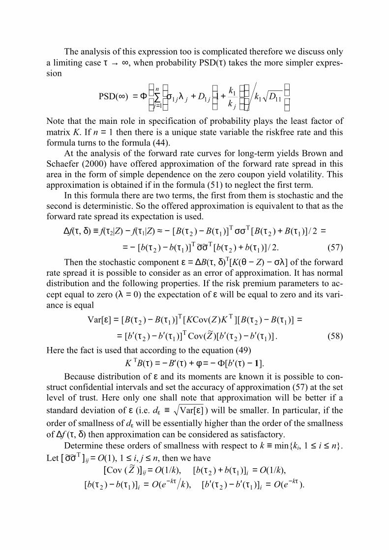
The analysis of this expression too is complicated therefore we discuss only a limiting case τ → ∞, when probability PSD(τ) takes the more simpler expres-sion

PSD(∞) = Φ

++λσ∑

=111

1

111 1 Dk

kkD

n

j jjjj .

Note that the main role in specification of probability plays the least factor of matrix K. If n = 1 then there is a unique state variable the riskfree rate and this formula turns to the formula (44).

At the analysis of the forward rate curves for long-term yields Brown and Schaefer (2000) have offered approximation of the forward rate spread in this area in the form of simple dependence on the zero coupon yield volatility. This approximation is obtained if in the formula (51) to neglect the first term.

In this formula there are two terms, the first from them is stochastic and the second is deterministic. So the offered approximation is equivalent to that as the forward rate spread its expectation is used.

∆f(τ, δ) ≡ f(τ2|Z) − f(τ1|Z) ≈ − 2/)]()([)]()([ 12TT

12 τ+τσστ−τ BBBB =

= − .2/)]()([~~)]()([ 12TT

12 τ+τσστ−τ bbbb (57) Then the stochastic component ε = ∆В(τ, δ)Т[K(θ − Z) − σλ] of the forward

rate spread it is possible to consider as an error of approximation. It has normal distribution and the following properties. If the risk premium parameters to ac-cept equal to zero (λ = 0) the expectation of ε will be equal to zero and its vari-ance is equal

Var[ε] = )]()(][)(Cov[)]()([ 12TT

12 τ−ττ−τ BBKZKBB =

= )]()()[~(Cov)]()([ 12T

12 τ′−τ′τ′−τ′ bbZbb . (58) Here the fact is used that according to the equation (49)

K ТB(τ) = − B′(τ) + φ = − Ф[b′(τ) − 1]. Because distribution of ε and its moments are known it is possible to con-

struct confidential intervals and set the accuracy of approximation (57) at the set level of trust. Here only one shall note that approximation will be better if a standard deviation of ε (i.e. dε ≡ ]Var[ε ) will be smaller. In particular, if the order of smallness of dε will be essentially higher than the order of the smallness of ∆f (τ, δ) then approximation can be considered as satisfactory.

Determine these orders of smallness with respect to k ≡ min{ki, 1 ≤ i ≤ n}. Let [ T~~σσ ] ij = О(1), 1 ≤ i, j ≤ n, then we have

[Cov ( Z~ )] ij = О(1/k), ibb )]()([ 12 τ+τ = О(1/k),

ibb )]()([ 12 τ−τ = ),( keO kτ− ibb )]()([ 12 τ′−τ′ = ).( τ−keO

Therefore orders of smallness of forward rate spread ∆f (τ, δ) and errors of its approximation dε have orders

∆f(τ, δ) = ),( 2keO kτ− dε = ).( keO kτ− (59)

So dε /∆f(τ, δ) = )( 23kO . For example, at k ≤ 0,2154 the relative error will be less than 10 %.

Gaussian model: the empirical analysis

Consider now a problem of determination of forward rates by experimental

data. We accept as a basis the data resulted by Brown and Schaefer (2000) for two-factor Gaussian model. They contain there in Table 1 (Standard Deviation of weekly changes (% p.a.) in zero coupon yields derived from US Treasury STRIP prices) and in Table А2 (Estimated Mean Reversion Coefficients and Correlation Coefficient) for three time periods: 88 – 94, 88 – 91 and 91 – 94. For convenience the data on standard deviations of zero coupon yield from Brown and Schaefer (2000) are resulted here in Table 4 in columns with indexes YE1, YE2, YE3. Estimations of factors k1, k2 and correlation coefficient ρ of the state variables from Brown and Schaefer (2000) are resulted here in Table 5.

Table 4

Standard deviation of zero coupon yield (empirical YE and determined from model YM)

Period 88 – 94 88 – 91 91 – 94 88 – 94 88 – 91 91 – 94

Maturity τ (years) YE1 YE2 YE3 YM1 YM2 YM3

2 0,991 1,002 0,927 1,031 1,022 1,006 3 1,030 1,001 1,015 1,001 0,983 0,986 5 0,994 0,958 1,012 0,951 0,927 0,949 7 0,904 0,871 0,932 0,908 0,885 0,913 10 0,857 0,845 0,878 0,854 0,837 0,863 15 0,733 0,719 0,755 0,778 0,773 0,786 20 0,686 0,694 0,684 0,714 0,717 0,719 25 0,684 0,722 0,649 0,657 0,668 0,659

Table 5

Estimations of factors k1, k2 and correlation coefficient ρρρρ

of state variables Period 88 – 94 88 – 91 91 – 94

k1 0,0393 0,0328 0,0417 k2 0,2060 0,3340 0,1260 ρ – 0,2540 – 0,1630 – 0,5560

In order to write the results in more convenient form present the covariance

matrix )~(Cov Z and the vector b(τ) as

)~(Cov Z = ,2221

2121

ρρ

DDDDDD b(τ) = .

)()(

)1()1(

2

1

2

12

1

ττ

≡

−−

τ−

τ−

bb

keke

k

k (60)

Then the zero coupon yield variance according to the formula (56) can be presented as

Var[у(τ)] = 2T /)]()~(Cov)([ τττ bZb =

= [b1(τ)2D12 + b2(τ)2D2

2 + 2 b1(τ)b2(τ)D1D2ρ]/τ2. (61) Let VЕ(τ) be a variance that is calculated as a square of a standard deviation

from columns YE of Table 4. Form a square of a difference S(τ) = (VЕ(τ) – [b1(τ)2D1

2 + b2(τ)2D22 + 2 b1(τ)b2(τ)D1D2ρ]/τ2)2.

In this expression the functions b1(τ) and b2(τ) are calculated by the formula (60) for coefficients from Table 5, the correlation coefficient ρ is used also from Table 5. For one of three periods we form the sum Q of squares S(τ) and mini-mize it on values D1, D2, i.e.

Q = min)(21,

25

2 →τ∑

=τDDS .

Such procedure of the Least Squares Method (LSM) allow to determine D1, D2 and hence the covariance matrix ).~(Cov Z It is known from the formula (56) that

[Cov( Z~ )] ij = ,]~~[ T

ji

ij

kk +σσ

1 ≤ i, j ≤ n.

From here with the help of the data of Table 5 it is possible to determine elements of a matrix T~~σσ and by the formula (57) we can determine the ap-proximation of forward rate spread.

Note that such procedure uses a simple LSM to determine the elements of the covariance matrix )~(Cov Z . Probably the application of more exact methods (for example, the Generalized Method of the Moments) will allow to receive more exact results.

At last we note that the described procedure is based on state variables Z~ and does not demand an estimation of a vector φ, through which the riskfree in-terest rate is determined. It is important advantage of such definition of state variables at practical calculations.

In the Table 6 the estimates of elements of the covariance matrix )~(Cov Z and size of the squares sum Q corresponding to them are submitted.

Last three columns with indexes YM of Table 4 contain values of standard deviations of zero coupon yield that are calculated by the formula (61) with use of the data of Table 6. Figure 4 is an illustration of the data of Table 4.

Table 6

Elements of covariance matrixes (60) of state variables

Period 88 - 94 88 – 91 91 - 94

D1 1,0650 0,9912 1,0764 D2 0,6669 0,7430 0,0565

Q 0,0246 0,0203 0,0486

Fig. 4. Standard deviations of zero coupon yields SD(Y) for US Treasury STRIP prices of Table 1 from Brown and Schaefer (2000) (YE) and calculated on the basis

of their data by the formula (61) (YM).

Matrixes )~(Cov Z and T~~σσ that are calculated according to formulae (56) and the data of Table 6 for the corresponding periods have the forms that are presented in Table 7.

0,6

0,7

0,8

0,9

1

1,1

0 5 10 15 20 25τ

SD(Y

)

YE1 YE2 YE3 YM1 YM2 YM3

Table 7 Matrixes )~(Cov Z and ,~~ Tσσ calculated

on the basis of the data of table 6

Period Matrix )~(Cov Z Matrix T~~σσ

88 - 94

−

−4448,01804,01804,01342,1

−

−1832,00443,00443,00892,0

88 – 91

−

−5522,01201,01201,09826,0

−

−3689,00440,00440,00645,0

91 - 94

−

−00319,00338,0

0338,01588,1

−

−000804,000567,0

00567,0096643,0

The Figure 5 shows the probabilities PSD(τ) for two factor models with parameters from Tables 5 and 7 if the risk premium parameters λ are zero.

The approximation of the forward rate spread calculated by the formula (57) for τ2 = 25, τ1 = 15 and its absolute (see the formula (58)) and relative er-rors are submitted in Table 8. From this table it follows, that the approximation offered by Brown and Schaefer (2000) for data of Tables 4 and 5 is valid with accuracy about 4 %.

Fig. 5. The probabilities PSD(τ) for the two factor Gaussian models for data from Brown & Schaefer (2000). The plots according to

the periods 88 – 94 (P1), 88 – 91 (P2) and 91 – 94 (P3).

0,5

0,6

0,7

0,8

0,9

1

0 0,5 1 1,5 2 2,5τ

PSD

P1 P2 P3

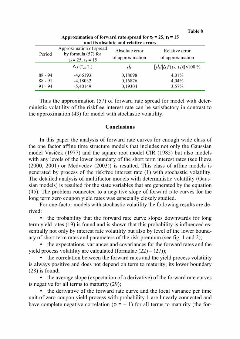
Table 8 Approximation of forward rate spread for ττττ2 ==== 25, ττττ1 ==== 15

and its absolute and relative errors

Period Approximation of spread

by formula (57) for τ2 = 25, τ1 = 15

Absolute error of approximation

Relative error of approximation

∆ f (τ2, τ1) dε [dε/|∆ f (τ2, τ1)|]×100 % 88 - 94 -4,66193 0,18698 4,01% 88 - 91 -4,18032 0,16876 4,04% 91 - 94 -5,40149 0,19304 3,57%

Thus the approximation (57) of forward rate spread for model with deter-

ministic volatility of the riskfree interest rate can be satisfactory in contrast to the approximation (43) for model with stochastic volatility.

Conclusions

In this paper the analysis of forward rate curves for enough wide class of

the one factor affine time structure models that includes not only the Gaussian model Vasiček (1977) and the square root model CIR (1985) but also models with any levels of the lower boundary of the short term interest rates (see Ilieva (2000, 2001) or Medvedev (2003)) is resulted. This class of affine models is generated by process of the riskfree interest rate (1) with stochastic volatility. The detailed analysis of multifactor models with deterministic volatility (Gaus-sian models) is resulted for the state variables that are generated by the equation (45). The problem connected to a negative slope of forward rate curves for the long term zero coupon yield rates was especially closely studied.

For one-factor models with stochastic volatility the following results are de-rived:

• the probability that the forward rate curve slopes downwards for long term yield rates (19) is found and is shown that this probability is influenced es-sentially not only by interest rate volatility but also by level of the lower bound-ary of short term rates and parameters of the risk premium (see fig. 1 and 2);

• the expectations, variances and covariances for the forward rates and the yield process volatility are calculated (formulae (22) – (27));

• the correlation between the forward rates and the yield process volatility is always positive and does not depend on term to maturity; its lower boundary (28) is found;

• the average slope (expectation of a derivative) of the forward rate curves is negative for all terms to maturity (29);

• the derivative of the forward rate curve and the local variance per time unit of zero coupon yield process with probability 1 are linearly connected and have complete negative correlation (ρ = − 1) for all terms to maturity (the for-

mulae (32) and (33)); the same results are obtained for the forward rate spread and the local variance of yield process (the formulae (39) and (40));

• the approximation of the forward rate spread (43) with the help of a lo-cal variance is reduced to change of the spread expectation more than on 30 % and at real cases cannot be recommended for models with stochastic volatility for any terms to maturity.

For one factor models with deterministic volatility (Gaussian models) • the probability that the forward rate curve slopes downwards for long

term yield rates (the formula (44)) is found; • this probability always is more 0,5, increases as the term to maturity in-

creases but has the upper boundary that is dependent on the interest rate volatil-ity (table 3, figure 3);

• in the mean the slope of the forward rate curve is negative independent on term to maturity.

For multifactor Gaussian models • the representation of state variable process in the explicit form is de-

rived and its covariance matrix is found (formula (46); • the modification of state variables simplifying the analysis and conven-

ient for practical application is offered (formulae (53) – (56)); • it is shown that the approximation offered by Brown and Schaefer

(2000) is reduced to that as the forward rate spread it is accepted its expectation therefore the error of approximation is its stochastic component (formulae (51), (57));

• the estimation of accuracy of such approximation (59) is found; • on the basis of the numerical data from Brown and Schaefer (2000) the

analysis two factor Gaussian models (Table 4-7) is carried out and it is shown that for this case the relative error of approximation is about 4 % (table 8).

The approximation of Brown and Schaefer for forward rate spread for model with deterministic volatility of the riskfree interest rate can be satisfactory used in contrast to that approximation for model with stochastic volatility.

References

Aït-Sahalia, Y. (1996) Nonparametric Pricing of Interest Rate Derivative Securities.

Econometrica 64, 527–560. Ait-Sahalia, Y. (1999) Transition densities for interest rate and nonlinear diffusions. Journ. of

Finance 54, 1361-1395. Bali, T. G. (1999) An Empirical Comparison of Continuous Time Models of the Short Term

Interest Rate. Journ. of Futures Markets 19, 777–797. Brown, R. H. and Schaefer, S. M. (1994) Interest Rate Volatility and Shape of the Term

Structure. Phil. Trans. R. Soc. Lond. A 347, 563–576. Brown, R. H. and Schaefer, S. M. (2000) Why Long Term Forward Interest Rates (Almost)

Always Slope Downalds. Working paper. London Business School.

Christiansen Ch. (2001) Long Maturity Forward Rates. Working paper. The Aarhus School of Business.

CIR: Cox, J. C., Ingersoll, J. E., and Ross, S. A. (1979) Duration and the Measurement of Basis Risk. Journ. Business 52, 51–61.

CIR: Cox, J. C., Ingersoll J. E., and Ross, S. A. (1985) A Theory of the Term Structure of Interest Rate. Econometrica 53, 385–467.

CKLS: Chan, K. C., Karolyi, G. A., Longstaff, F. A., and Sanders A. S. (1992) An Empirical Comparison of Alternative Models of the Short-Term Interest Rate. Journ. of Finance 47, 1209–1227.

Dai Q. and Singleton, K. J. (2000) Specification Analysis of Affine Term Structure Models. Journal of Finance 55(5), 1943-1978.

Duffie, D. and Kan, R. (1996) A Yield-Factor Model of Interest Rates, Mathematical Finance 6, 379–406.

Duffie, D. and Singleton, K. J. (1997) An Econometric Model of the Term Structure of Inter-est-Rate Swap Yields. Journ. of Finance 52, 1287–1321.

Feller, W. (1951) Two singular diffusion problems. Annals of Mathematics. Vоl. 54, No. 1. Р. 173–182.

Gibbons, M. R. and Ramaswamy, K. (1993) A Test of the Cox, Ingersoll, and Ross Model of the Term Structure. Review of Financial Studies 6, 619–658.

Heath D., Jarrow R., Morton A. (1992) Bond Pricing and Term Structure of Interest Rates: New Methodology for Contingent Claims Valuation. Econometrica 60, 77–105.

Hull, J. C. (1993) Options, Futures, and Other Derivative Securities. Prentice Hall, Engle-wood Cliffs.

Ilieva, N. G. (2000) The Comparative Analysis of the Term Structure Models of the Affine Yield Class. Proc. of the 10-th Intern. AFIR Symposium. Tromso, 367–393.

Ilieva, N. G. (2001) Use of Mathematical Models of the Interest Rate Processes for the Analy-sis of Yield Time Series. Proc. of the 6-th Intern. Conf. “Computer Data Analysis and Modeling”, Minsk, 157–164.

Kortanek, K. O. and Medvedev, V. G. (2001) Building and Using Dynamic Interest Rate Models. John Wiley & Sons, New York.

Medvedev, G. A. (2003) Properties of yield curves and forward curves for affine term struc-ture models. Proc. of the 13-th Intern. AFIR Symposium. Maastricht, 461–492.

Pearson, N. D. and Sun, T.-S. (1994) Exploiting the Conditional Density in Estimating the Term Structure: An Application to the Cox, Ingersoll, and Ross model. Journ. of Fi-nance 49, 1279–1304.

Sun, T.-S. (1992) Real and Nominal Interest Rates: A Discrete-Time Model and Its Continu-ous-Time Limit. Review of Financial Studies 5, 581–611.

Vasiček, O. A. (1977) An Equilibrium Characterization of the Term Structure. Journ. of Fi-nancial Economics 5, 177–188.