formalization of resolution calculus in isabelle - dtu … · summary (english)...
TRANSCRIPT
Formalization ofResolution Calculus
in Isabelle
Anders Schlichtkrull
Kongens Lyngby 2015
Semantic gardener cutting a semantic tree.Drawing by Inger Schlichtkrull
Technical University of DenmarkDepartment of Applied Mathematics and Computer ScienceRichard Petersens Plads, building 324,2800 Kongens Lyngby, DenmarkPhone +45 4525 [email protected]

Summary (English)
The goal of this thesis is to formalize the resolution calculus for first-order logicand prove it sound and complete in the Isabelle proof assistant. The resolutioncalculus is a successful proof system, i.e. a system that can prove propertiesabout mathematics, computer science, and much more. Two desirable prop-erties for proof systems are soundness and completeness, because they expressthat every proof in the system is correct and that the system can prove all validformulas of the given logic. Isabelle is a proof assistant i.e. a computer programthat can help its user in conducting proofs, and which can check their correct-ness. By proving these properties in Isabelle we will gain confidence in theirvalidity.
The thesis formalizes the resolution calculus and its soundness in Isabelle. Thesoundness proof is thorough and makes explicit the interplay of syntax andsemantics. Likewise, the thesis formalizes two major steps of proving the reso-lution calculus complete, namely König’s lemma, and Herbrand’s theorem. Thethe next two major steps of proving completeness are the lifting lemma andcompleteness itself. The thesis discusses flaws in informal proofs of the liftinglemma from the literature, which make its formalization difficult. With theseflaws in mind, the thesis discusses two possibilities for a formalization of thelemma. The thesis also describes thoroughly, albeit informally, how to finishthe completeness proof. Finally, the thesis suggests possibilities for future workon the formalization of proof systems.

ii
Summary (Danish)
Målet for denne afhandling er at formalisere resolutionskalkulen for førsteor-denslogik samt at bevise at den er sund og fuldstændig i bevisassistenten Isa-belle. Resolutionskalkulen er et succesfuldt bevissystem, dvs. et system der kanbevise egenskaber om matematik, informatik og meget mere. To ønskværdigeegenskaber for bevissystemer er sundhed og fuldstændighed, fordi de udtrykkerat ethvert bevis, som systemet laver, er korrekt, og at systemet kan bevise allegyldige formler i den givne logik. Isabelle er en bevisassistent, dvs. et computerprogram der kan hjælpe sin bruger med at føre beviser, og som kan kontrollerederes korrekthed. Ved at bevise sundhed og fuldstændighed vil vi øge vores tiltrotil dem.
Afhandlingen formaliserer resolutionskalkulen og dens sundhed i Isabelle. Sund-hedsbeviset er grundigt og gør samspillet mellem syntaks og semantik helt ty-delig. Ligeledes formaliserer afhandlingen to store skridt mod et bevis af fuld-stændighed, nemlig Königs hjælpesætning og Herbrands sætning. De næste tostore skridt er løftehjælpesætningen og selve fuldstændigheden. Afhandlingendiskuterer mangler i uformelle beviser fra litteraturen, som gør det svært atformalisere dem. Med disse mangler for øje diskuterer afhandlingen to mulighe-der for at formalisere hjælpesætningen. Afhandlingen beskriver også grundigt,omend uformelt, hvordan beviset for resolutionskalkulens fuldstændighed kangøres færdigt. Slutteligt foreslår specialet muligheder for fremtidigt arbejde påformaliseringer af bevissystemer.

iv

Preface
This thesis was prepared at DTU Compute in fulfillment of the requirements foracquiring an M.Sc. in Engineering. The thesis deals with the formalization ofthe resolution calculus in the Isabelle proof assistant. The thesis is for 30 ECTSand was written in the period from 31 March 2015 to 31 August 2015. JørgenVilladsen served as supervisor on the thesis, and Jasmin Christian Blanchetteserved as co-supervisor.
The prerequisites for understanding the thesis are knowledge of set theory aswell as mathematical proving and reasoning. It is also advantageous to haveknowledge of functional programming, and first-order logic. Knowledge of for-malization work and proof assistants is not required.
Lyngby, 31 August 2015
Anders Schlichtkrull

vi

Acknowledgements
I would like to thank my thesis supervisors Jørgen Villadsen and Jasmin Chris-tian Blanchette for their guidance and feedback during the process. Jørgen wasmy personal tutor on the Honors Program, and introduced me to the world ofIsabelle. I was very fortunate to get Jasmin as supervisor for my thesis. Hisinsight in formalizations of proof systems was exceedingly valuable, and so washis thorough comments on my work.
Additionally, I would like to give special thanks to Dmitriy Traytel, who alsoprovided me with much guidance and feedback. For all practical purposes heserved as a third supervisor on the thesis, and his input was remarkably helpful.
I would also like to thank Tobias Nipkow, Peter Lammich, and Johannes Hölzl,for their teaching in the excellent course “Semantics” at TUM (Technische Uni-versität München). I was so lucky to attend the course during my semesterabroad at the university. The course made me appreciate formal semantics, andtaught me the craft of formal theorem proving.
Furthermore, I would like to thank Melvin Fitting for his textbook on logicand automated theorem proving. This book together with Stefan Berghofer’sformalization of its completeness proof helped spark my interest in completeness.For this, I would also like to thank Stefan Berghofer. His enumeration of termsis also used in my thesis, and I took much inspiration from his work.
Writing a thesis during the summer holidays can for many reasons be a chal-lenge. I would therefore like to thank my fellow student Andreas Viktor Hessfor company, while we were writing our theses.

viii
I would also like to thank my parents Peter and Inger Schlichtkrull for theirsupport. Likewise, I would like to thank my family, my friends, and my fellowresidents of the Professor Ostenfeld Dormitory. Finally, I would like to thankmy mother Inger Schlichtkrull for the title and colophon page drawings.

ix

x Contents
Contents
Summary (English) i
Summary (Danish) iii
Preface v
Acknowledgements vii
1 Introduction 1
2 Preliminaries and Theory Background 52.1 First-order Logic . . . . . . . . . . . . . . . . . . . . . . . . . . . 52.2 Syntax . . . . . . . . . . . . . . . . . . . . . . . . . . . . . . . . . 92.3 Semantics . . . . . . . . . . . . . . . . . . . . . . . . . . . . . . . 10
2.3.1 Interpretations . . . . . . . . . . . . . . . . . . . . . . . . 112.3.2 Terms . . . . . . . . . . . . . . . . . . . . . . . . . . . . . 112.3.3 Formulas . . . . . . . . . . . . . . . . . . . . . . . . . . . 12
2.4 Proof Systems . . . . . . . . . . . . . . . . . . . . . . . . . . . . . 142.5 Soundness and Completeness . . . . . . . . . . . . . . . . . . . . 162.6 Prenex Conjunctive Normal Form . . . . . . . . . . . . . . . . . . 162.7 Clausal Forms . . . . . . . . . . . . . . . . . . . . . . . . . . . . . 172.8 Substitutions . . . . . . . . . . . . . . . . . . . . . . . . . . . . . 182.9 Resolution . . . . . . . . . . . . . . . . . . . . . . . . . . . . . . . 192.10 Isabelle . . . . . . . . . . . . . . . . . . . . . . . . . . . . . . . . 222.11 HOL . . . . . . . . . . . . . . . . . . . . . . . . . . . . . . . . . . 23
3 Analysis of the Problem 253.1 Resolution Calculus in the Literature . . . . . . . . . . . . . . . . 25
3.1.1 Binary Resolution with Factoring . . . . . . . . . . . . . . 25

xii CONTENTS
3.1.2 General Resolution . . . . . . . . . . . . . . . . . . . . . . 263.1.3 Resolution Suited for Hand Calculation . . . . . . . . . . 273.1.4 Other Variants of the Resolution Calculus . . . . . . . . . 27
3.2 Soundness and Completeness Proofs . . . . . . . . . . . . . . . . 273.2.1 Semantic Trees . . . . . . . . . . . . . . . . . . . . . . . . 283.2.2 Consistency Properties . . . . . . . . . . . . . . . . . . . . 333.2.3 Unified Completeness . . . . . . . . . . . . . . . . . . . . 34
3.3 Other Considerations . . . . . . . . . . . . . . . . . . . . . . . . . 363.4 Other Presentations . . . . . . . . . . . . . . . . . . . . . . . . . 373.5 The Approach of This Project . . . . . . . . . . . . . . . . . . . . 37
4 Formalization: Logical Background 394.1 Terms . . . . . . . . . . . . . . . . . . . . . . . . . . . . . . . . . 394.2 Literals . . . . . . . . . . . . . . . . . . . . . . . . . . . . . . . . 404.3 Clauses . . . . . . . . . . . . . . . . . . . . . . . . . . . . . . . . 444.4 Collecting Variables . . . . . . . . . . . . . . . . . . . . . . . . . 454.5 Ground . . . . . . . . . . . . . . . . . . . . . . . . . . . . . . . . 464.6 Semantics . . . . . . . . . . . . . . . . . . . . . . . . . . . . . . . 474.7 Substitutions . . . . . . . . . . . . . . . . . . . . . . . . . . . . . 51
4.7.1 Composition . . . . . . . . . . . . . . . . . . . . . . . . . 534.7.2 Unifiers . . . . . . . . . . . . . . . . . . . . . . . . . . . . 55
5 Formalization: Resolution Calculus and Soundness 575.1 The Resolution Calculus . . . . . . . . . . . . . . . . . . . . . . . 575.2 Soundness of the Resolution Rule . . . . . . . . . . . . . . . . . . 59
5.2.1 Soundness of Substitution . . . . . . . . . . . . . . . . . . 595.2.2 Soundness of Simple Resolution . . . . . . . . . . . . . . . 615.2.3 Combining the Rules . . . . . . . . . . . . . . . . . . . . . 625.2.4 Applicability . . . . . . . . . . . . . . . . . . . . . . . . . 63
5.3 Soundness of Resolution Derivations . . . . . . . . . . . . . . . . 64
6 Formalization: Completeness 656.1 Herbrand Terms . . . . . . . . . . . . . . . . . . . . . . . . . . . 656.2 Enumerations . . . . . . . . . . . . . . . . . . . . . . . . . . . . . 676.3 Semantic Trees and Partial Interpretations . . . . . . . . . . . . . 686.4 König’s Lemma . . . . . . . . . . . . . . . . . . . . . . . . . . . . 706.5 Semantics of Partial Predicate Denotations . . . . . . . . . . . . 736.6 Herbrand’s Theorem . . . . . . . . . . . . . . . . . . . . . . . . . 75
6.6.1 Building a Model . . . . . . . . . . . . . . . . . . . . . . . 756.6.2 Proving Herbrand’s Theorem . . . . . . . . . . . . . . . . 77
6.7 Lifting Lemma . . . . . . . . . . . . . . . . . . . . . . . . . . . . 796.8 Completeness . . . . . . . . . . . . . . . . . . . . . . . . . . . . . 79
7 Examples 83

CONTENTS xiii
8 Discussion 878.1 Proving the Lifting Lemma . . . . . . . . . . . . . . . . . . . . . 87
8.1.1 A Proof From the Literature . . . . . . . . . . . . . . . . 888.1.2 Another Resolution Calculus . . . . . . . . . . . . . . . . 918.1.3 The Unification Algorithm . . . . . . . . . . . . . . . . . 928.1.4 Recommended Approach . . . . . . . . . . . . . . . . . . 92
8.2 Formalizing a Logical System in a Logical System . . . . . . . . . 928.3 Automatic Theorem Proving . . . . . . . . . . . . . . . . . . . . 938.4 Societal Perspective . . . . . . . . . . . . . . . . . . . . . . . . . 948.5 Lessons Learned . . . . . . . . . . . . . . . . . . . . . . . . . . . 948.6 Reflections on the Thesis . . . . . . . . . . . . . . . . . . . . . . . 95
9 Conclusions 979.1 Results . . . . . . . . . . . . . . . . . . . . . . . . . . . . . . . . . 979.2 Contribution . . . . . . . . . . . . . . . . . . . . . . . . . . . . . 989.3 Future Work . . . . . . . . . . . . . . . . . . . . . . . . . . . . . 98
A Formalization Code: TermsAndLiterals.thy 101A.1 BSD Software License . . . . . . . . . . . . . . . . . . . . . . . . 101A.2 Terms and Literals . . . . . . . . . . . . . . . . . . . . . . . . . . 102
A.2.1 Enumerating datatypes . . . . . . . . . . . . . . . . . . . 103
B Formalization Code: Tree.thy 109B.1 Paths . . . . . . . . . . . . . . . . . . . . . . . . . . . . . . . . . 109B.2 Branches . . . . . . . . . . . . . . . . . . . . . . . . . . . . . . . . 110B.3 Internal Nodes . . . . . . . . . . . . . . . . . . . . . . . . . . . . 112B.4 Deleting Nodes . . . . . . . . . . . . . . . . . . . . . . . . . . . . 114B.5 Possibly Infinite Trees . . . . . . . . . . . . . . . . . . . . . . . . 117B.6 Infinite Paths . . . . . . . . . . . . . . . . . . . . . . . . . . . . . 117B.7 König’s Lemma . . . . . . . . . . . . . . . . . . . . . . . . . . . . 118
C Formalization Code: Resolution.thy 121C.1 Terms and literals . . . . . . . . . . . . . . . . . . . . . . . . . . 121C.2 Clauses . . . . . . . . . . . . . . . . . . . . . . . . . . . . . . . . 122C.3 Semantics . . . . . . . . . . . . . . . . . . . . . . . . . . . . . . . 123
C.3.1 Semantics of Ground Terms . . . . . . . . . . . . . . . . . 123C.4 Substitutions . . . . . . . . . . . . . . . . . . . . . . . . . . . . . 124
C.4.1 The Empty Substitution . . . . . . . . . . . . . . . . . . . 125C.4.2 Substitutions and Ground Terms . . . . . . . . . . . . . . 125C.4.3 Composition . . . . . . . . . . . . . . . . . . . . . . . . . 126
C.5 Unifiers . . . . . . . . . . . . . . . . . . . . . . . . . . . . . . . . 128C.5.1 Most General Unifiers . . . . . . . . . . . . . . . . . . . . 129
C.6 Resolution . . . . . . . . . . . . . . . . . . . . . . . . . . . . . . . 130C.7 Soundness . . . . . . . . . . . . . . . . . . . . . . . . . . . . . . . 131
xiv CONTENTS
C.8 Enumerations . . . . . . . . . . . . . . . . . . . . . . . . . . . . . 134C.9 Herbrand Interpretations . . . . . . . . . . . . . . . . . . . . . . 134C.10 Partial Interpretations . . . . . . . . . . . . . . . . . . . . . . . . 135
C.10.1 Semantic Trees . . . . . . . . . . . . . . . . . . . . . . . . 138C.11 Herbrand’s Theorem . . . . . . . . . . . . . . . . . . . . . . . . . 139C.12 Lifting Lemma . . . . . . . . . . . . . . . . . . . . . . . . . . . . 144C.13 Completeness . . . . . . . . . . . . . . . . . . . . . . . . . . . . . 144
D Formalization Code: Examples.thy 147
E Chang and Lee’s Lifting Lemma 155
Bibliography 159

Chapter 1
Introduction
Logic is the study of reasoning. Given some knowledge, we want to study whatnew knowledge we can derive from it. This has many different applications.For instance, it can be used to reason about a computer program for alertingthe crew of an airplane if it is diverging from its expected flight path during alanding. For instance, using logic, one can derive useful properties e.g. that analert is issued before a collision.
In our everyday life, different people can have different ideas of what they findlogical and what they do not, but in mathematics and computer science this ismostly not the case. Most mathematicians, computer scientists, and engineerscan agree on which general logical derivations are correct to make. If we take outa set of these and only use these in combination to construct other derivationsthen we have a proof system. The chosen set is called the rules of the proofsystem.
Proof systems can be implemented as computer programs called automated the-orem provers. The approach of automatic theorem provers is to take sentencesas input, and prove them completely automatically. Another approach is proofassistants in which the user guides the computer program towards the proof.We can therefore get a computer to prove properties about an airplane alert-ing computer program [CM00]. In this way, we increase our confidence in theprogram.

2 Introduction
The resolution calculus is one of the most successful proof systems implementedas an automatic theorem prover. The resolution calculus and an extension calledsuperposition are for instance used in the computer programs E [Sch13], SPASS[WDF+09], and Vampire [RV99]. These provers have participated in CASC,which is the world championship of automated theorem provers. E, SPASS andVampire have each won in several categories of the competition over the years[SS15, Sut14].
Experience has shown that humans, and even mathematicians, make mistakeswhen reasoning. A good example of this is the purported proof of the four colorconjecture from by Kempe in 1879. The proof convinced many mathematicians,but turned out to be fatally flawed, and relied on an assumption that hadcounter-examples [Hea80].
In proof systems, larger derivations are build up from the few small rules thatwe agree on, and so the proof system ensures that the derivation is correct.Therefore, a proof system would not have accepted Kempe’s proof. Since theproof was found to have errors, work has been going on to make new and correctproofs of the conjecture. A thorough proof was made in 2006 in the proof systemand proof assistant of Coq [Gon08].
However, if we are to trust a proof system, it is important that its rules areactually correct and sound. It is also important that our proof system is suf-ficiently strong so that it can prove the properties we want to establish. Thestrongest proof systems are called complete.
The classical approach to show that a system is sound and complete is to makea mathematical proof of this in a natural language such as English. A recentdevelopment is the approach of complementing this with the use of proof as-sistants. Proof assistants can help their users in conducting proofs, and theycheck the correctness of proofs. The process of specifying some mathematicalobjects or systems in a proof assistant and proving properties about them iscalled formalization.
The purpose of this project is to investigate how one can formalize the proofsystem called the resolution calculus for first-order logic as well as prove itssoundness and completeness in the Isabelle proof assistant.
• Chapter 2 introduces the first-order logic, the resolution calculus, the Isa-belle proof assistant, and its underlying logic called higher-order logic.
• Chapter 3 analyzes a number of different approaches to formalizing proofsystems, as well as proving their soundness and completeness.
3
• Chapters 4 to 6 present my approach to formalizing the resolution calcu-lus. They describe the definitions and the proofs as well as how they areformalized. Moreover, they explain the choices I had to make and suggestsalternatives.
– Chapter 4 formalizes background theory.
– Chapter 5 formalizes the resolution calculus and its soundness.
– Chapter 6 formalizes König’s lemma and Herbrand’s Theorem. Itthen explains how these results can be used to prove completeness.
• Chapter 7 shows a number of examples of derivations in the resolutioncalculus. These examples are also formalized.
• Chapter 8 discusses the strengths and weaknesses of my approach to theformalization. It also discusses different possibilities for future work onthe formalization.
• Chapter 9 concludes on my findings and suggests further work.

4 Introduction
Chapter 2
Preliminaries and TheoryBackground
This chapter explains the theory of first order logic and the Isabelle proof as-sistant that is necessary to understand this thesis. It explains first-order logic,the resolution calculus, the Isabelle proof assistant, and the higher order logicof Isabelle.
2.1 First-order Logic
Logic is the study of reasoning. Given some knowledge, we want to considerwhat new knowledge we can derive from it. An example is the following:
We know that
• The pyramids were built by Egyptians or the pyramids were built by aliens.
• The pyramids were not built by aliens.
and it follows that
6 Preliminaries and Theory Background
• The pyramids were built by Egyptians.
This example shows that we can reason logically about sentences in English.However, instead of considering logic about sentences English we now look atanother language called propositional logic. Sentences in this language are calledformulas. Propositional logic has several advantages over English. The most im-portant is that has a simpler syntax and semantics, but is still quite expressive.The language consists of propositions and logical connectives. An example of aproposition is “The pyramids were built by Egyptians”. In propositional logicwe represent propositions with letters, so instead of “The pyramids were built byEgyptians” we could just write E. Likewise we could chose that “the pyramidswere built by aliens” is denoted by A. Making such a choice is called an inter-pretation. Logical connectives then bind the propositions together. For instance“The pyramids were built by Egyptians or the pyramids were built by aliens” canbe written E∨A where ∨ is the connective that means “or”. Another connectiveis ¬, which gives the negation of a proposition, so “The pyramids were not builtby aliens” is written ¬A. Let us write the example above in the language ofpropositional logic.
We know that
• E ∨A
• ¬A
and thus it follows that
• E
By looking at this example we can realize that in this case, it does actuallynot matter what E and A means. We can choose another interpretation wheretheir meaning is something completely different, but if E ∨A is true and ¬A istrue then we can conclude that E is also true. Therefore, we say that E followslogically from E ∨A and ¬A. This is written as E ∨A,¬A |= E.
This is an important point in propositional logic. Propositional symbols such asE and A have no preconceived meaning. If we want to give them a meaning, weneed to provide an interpretation that says for each propositional symbol whatits meaning is.
Let us look at another example:
2.1 First-order Logic 7
We know that
• If it is raining on the priest then it is dripping on the perish clerk.
• It is raining on the priest.
and can thus it follows that
• It is dripping on the perish clerk.
We now let P denote “It is raining on the priest” and C denote “It is dripping onthe perish clerk”. We can now use the → connective to express “If it is rainingon the priest then it is dripping on the perish clerk” as P → C. Therefore, theexample is as follows:
We know that
• P → C
• P
and thus it follows that
• C
This derivation is again independent of our interpretation, and therefore weagain say that C is a logical consequence of P → C and P , i.e. P → C,P |= C.
A last example of logical consequence is the following:
We know that
• All men are mortal.
• Socrates is a man.
and thus it follows that:
• Socrates is mortal.
8 Preliminaries and Theory Background
We could try express it as A,B |= C, but this is wrong since we can let A denote2+2 = 4 and B denote 2 · 2 = 4 and C denote 2− 2 = 4. Even though it is truethat 2 + 2 = 4 and 2 · 2 = 4 it is not true that 2 − 2 = 4. We need a languagethat can capture the inner meaning of a proposition like “All men are mortal”,namely what it tells us about some individuals.
Therefore, we introduce the language of first-order logic (FOL). In this languagewe can express many thing such as for example a mathematical inequality “x >y”. We write it as g(x, y). Here, g is called a predicate and it says somethingabout the variables x and y. We can also represent expressions like “x+ π > xfor any x” as ∀x. g(p(x, π), x). Here ∀ is called the universal quantifier andexpresses “for all x”. We can let p denote the function that gives the sum of itsarguments, and π denote 3.14159.... Thus, we have predicates, functions andconstants in the language of first-order logic. Additionally we can use the logicalconnectives from the propositional logic. The variables, functions and constantscan symbolize anything - not just numbers. This is enough to express the aboveexample:
We know that
• ∀x. m(x)→ d(x)
• m(s)
and thus it follows that:
• d(s)
Here m(x) denotes “x is a man” and d(x) denotes “x is mortal” and s denotes“Socrates”. We expressed “All men are mortal” as “For any individual, if it isa man it is mortal” which is ∀x. m(x) → d(x) in first-order logic. “Socrates isa man” is m(s) and likewise “Socrates is mortal” is d(s). Like in the previousexample, we can realize that it actually does not matter what the meaning ofm, d and s are. As long as ∀x. m(x)→ d(x) and m(s) hold we can still concludethat d(s). So we know that d(s) follows logically from ∀x. m(x) → d(x) andm(s), which is written ∀x. m(x)→ d(x),m(s) |= d(s).
Like in propositional logic, it is again an important point that the predicatesymbols, constant symbols and function symbols have no preconceived meaning.To give them meaning we must provide a denotation of the predicate symbolsthat tells us what it means. Likewise, we need a denotation of constant symbolsand a denotation of function symbols. These denotations together are called
2.2 Syntax 9
an interpretation because they interpret the different symbol to give us theirmeaning.
2.2 Syntax
The above section gives the intuition about what we can express in first-orderlogic, and what the meaning of a formula in the language is. We have forinstance seen that ∨ corresponds to “or” in English and → corresponds to “if”and “then” in English. However, even simple words like “or” and “if” can meanslightly different things in different contexts. For instance, if I tell my fatherthat I want a bicycle or a Gameboy for my birthday, then I actually wish forboth of them. At the other hand, if I tell a bartender that I would like a beeror a cider then I only want one of them, and not both.
To remedy this we now express in a mathematically precise way the syntax andthe semantics of first-order logic. The syntax defines what we can write in thelanguage, and the semantics defines the meaning of those things we can write.
Firstly, first-order logic consists of terms. We have already seen some termssuch as x, y, s, π and more interestingly p(x, y). In fact, a term could be muchmore complicated such as f(g(x, y), h(i(x), z)).
Definition 2.1 A term is either
• A variable, x (or y, z, etc.), where x is a variable symbols.
• A function, e.g. f (or g, h, etc.) applied to a list of terms t1, ..., tn thatis: f(t1, ..., tn) where f is a function symbol. In this thesis we representsymbols by letters or strings of letters. A constant is a function applied tothe empty list of terms f() and is often written without the parentheses.
Secondly, first-order logic contains formulas. We have seen several formulas suchas ∀x. m(x)→ d(x) as well as m(s) and d(s). The formulas can contain logicalconnectives such as ∧. There are a few more than we have seen to far. Theycan be summarized in a table:

10 Preliminaries and Theory Background
Connective Short name Full name Subformulas∧ “and” conjunction conjuncts→ “if ... then ...” “only if” implication∨ “or” disjunction disjuncts↔ “if and only if” “iff” biimplication¬ “not” negation⊥ falsity> truth
We are now ready to define formulas.
Definition 2.2 A formula is either
• A predicate p applied to a list of terms t1, ..., tn that is: p(t1, ..., tn) wherep is a predicate symbol. This is called an atomic formula.
• The universal quantification of a formula F : ∀x. F where x is a variable.Any occurrence of x in F is said to be bound by the quantifier, unless it isbound by another quantifier inside of F .
• The existential quantification of a formula F : ∃x. F where x is a variable.Existential quantifiers bind occurrences of variables just like universal quan-tifiers.
• The negation of a formula F : ¬F .
• The conjunction of two formulas F1 and F2: F1 ∧ F2.
• The disjunction of two formulas F1 and F2: F1 ∨ F2.
• The implication from a formula F1 to a formula F2: F1 → F2.
• The biimplication between a formula F1 and a formula F2: F1 ↔ F2.
• Falsum: ⊥.
• Truth: >.
2.3 Semantics
Now that we have defined what we can write in FOL, that is, the syntax ofFOL, we are ready to define precisely what the meaning terms and formulas is,that is, the semantics of FOL.

2.3 Semantics 11
2.3.1 Interpretations
The meaning of a term is some object or element from the universe u of elementsabout which we wish to express something. u is a set of elements and could forinstance be the set of natural numbers, the set of all C programs or the set ofstreets in Copenhagen. As said, the function symbols do not have any particularmeaning. Therefore, we need to specify a denotation of the function symbols.A denotation of function symbols is a map that takes a function symbol and alist of elements of the universe and then returns an element of the universe.
Definition 2.3 A function denotation is a map of type function symbol ⇒u list⇒ u.
Likewise, we need a variable denotation.
Definition 2.4 A variable denotation is a map from variable symbols to ele-ments of the universe: variable symbol⇒ u.
Lastly, we introduce predicate denotations to describe the meaning of predicates.They are maps from predicate symbols and lists of elements of the universe intothe type bool consisting of true and false. The idea is that this map defines forwhich lists of elements the predicate is true, and for which it is false.
Definition 2.5 A predicate denotation is a map of type predicate symbol ⇒u list⇒ u.
As said, a predicate denotation together with a variable denotation is called aninterpretation.
2.3.2 Terms
Now we are ready to give meaning to terms by specifying a semantics. We dothis by introducing the semantic brackets, J and K, which recursively calculatethe meaning of the enclosed term. In other words, they evaluate the term.
Definition 2.6 Given a variable denotation E and a function denotation F ,we can evaluate terms as follows:
• JxKEF = E(x) if x is a variable symbol.
12 Preliminaries and Theory Background
• Jf(t1, ..., tn)KEF = F (f, [ Jt1KEF , ..., JtnKEF ])
Consider for instance the function denotation Fnat which maps the symbol zeroto the natural number 0, one to the natural number 1, the symbol s to thefunction that adds 1 to a number, add to addition and mul to multiplication.
Consider also the variable denotation Enat that maps x to 26 and y to five.
We evaluate add(mul(y, y), one())):
Jadd(mul(y, y), one()))KEnat
Fnat
= Fnat add J(mul(y, y))KEnat
FnatJone()KEnat
Fnat
= Jmul(y, y)KEnat
Fnat+ Jone()KEnat
Fnat
= Fnat mul (JyKEnat
Fnat, JyKEnat
Fnat) + Fnat one ()
= (JyKEnat
Fnat· JyKEnat
Fnat) + 1
= (Enat y · Enat y) + 1
= (5 · 5) + 1
= 26
2.3.3 Formulas
Likewise, we can define the semantics for formulas. We extends the semanticbrackets to cover also formulas. A formula expresses some claim that is eithertrue or false. Thus, when we evaluate a formula we get a value of type bool.
Firstly, we need to have a definition of what the logical connectives mean. Thisis always fixed and can be described by the following tables:
A B J∧K(A,B)true true truetrue false falsefalse true falsefalse false false
A B J→K(A,B)true true truetrue false falsefalse true truefalse false true
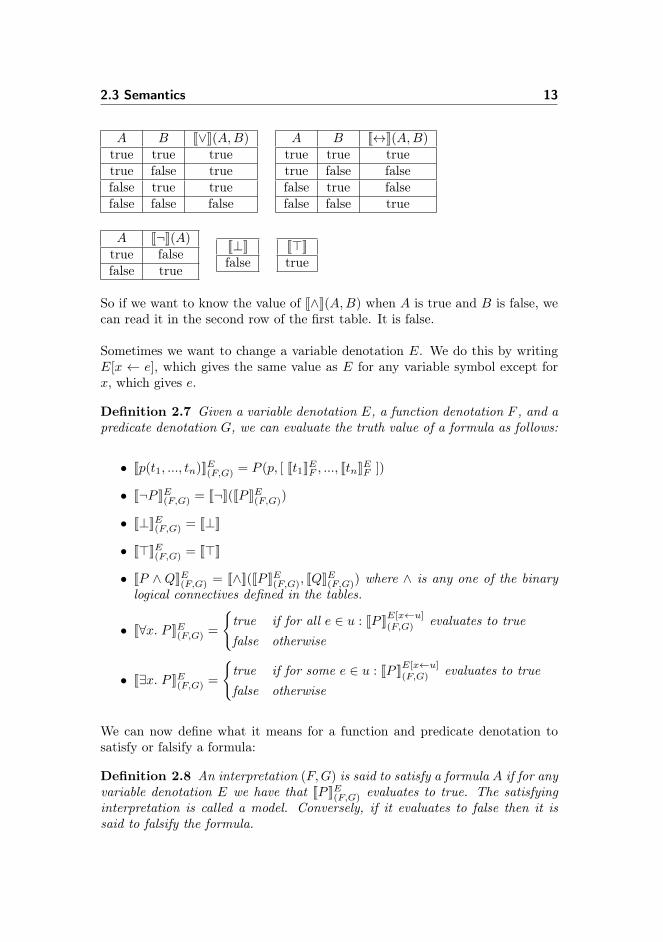
2.3 Semantics 13
A B J∨K(A,B)true true truetrue false truefalse true truefalse false false
A B J↔K(A,B)true true truetrue false falsefalse true falsefalse false true
A J¬K(A)true falsefalse true
J⊥Kfalse
J>Ktrue
So if we want to know the value of J∧K(A,B) when A is true and B is false, wecan read it in the second row of the first table. It is false.
Sometimes we want to change a variable denotation E. We do this by writingE[x ← e], which gives the same value as E for any variable symbol except forx, which gives e.
Definition 2.7 Given a variable denotation E, a function denotation F , and apredicate denotation G, we can evaluate the truth value of a formula as follows:
• Jp(t1, ..., tn)KE(F,G) = P (p, [ Jt1KEF , ..., JtnKEF ])
• J¬P KE(F,G) = J¬K(JP KE(F,G))
• J⊥KE(F,G) = J⊥K
• J>KE(F,G) = J>K
• JP ∧ QKE(F,G) = J∧K(JP KE(F,G), JQKE(F,G)) where ∧ is any one of the binarylogical connectives defined in the tables.
• J∀x. P KE(F,G) =
{true if for all e ∈ u : JP KE[x←u]
(F,G) evaluates to truefalse otherwise
• J∃x. P KE(F,G) =
{true if for some e ∈ u : JP KE[x←u]
(F,G) evaluates to truefalse otherwise
We can now define what it means for a function and predicate denotation tosatisfy or falsify a formula:
Definition 2.8 An interpretation (F,G) is said to satisfy a formula A if for anyvariable denotation E we have that JP KE(F,G) evaluates to true. The satisfyinginterpretation is called a model. Conversely, if it evaluates to false then it issaid to falsify the formula.
14 Preliminaries and Theory Background
We can also make it more clear what we mean when we talk of logical conse-quence and validity:
Definition 2.9 If any model of B1, ..., Bn is also a model of A then we say thatA is a logical consequence of B1, ..., Bn.
It is written B1, ..., Bn |= A
Definition 2.10 A formula A is said to be valid if any interpretation is a modelfor A.
It is written |= A
Likewise, we define equality and equisatisfiability which are concepts that comein handy when we want to rewrite formulas.
Definition 2.11 A formula A and a formula B are said to be equivalent if anymodel for A is also a model for B, and vice-versa.
It is written A ≡ B
Definition 2.12 A formula A and a formula B are said to be equisatisfiable ifthey have the property that:
A is satisfiable if and only if B is satisfiable.
2.4 Proof Systems
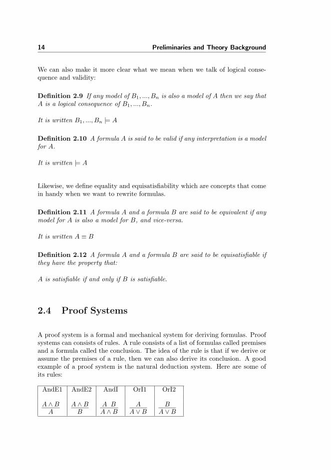
A proof system is a formal and mechanical system for deriving formulas. Proofsystems can consists of rules. A rule consists of a list of formulas called premisesand a formula called the conclusion. The idea of the rule is that if we derive orassume the premises of a rule, then we can also derive its conclusion. A goodexample of a proof system is the natural deduction system. Here are some ofits rules:
AndE1 AndE2 AndI OrI1 OrI2
A ∧BA
A ∧BB
A BA ∧B
AA ∨B
BA ∨B
2.4 Proof Systems 15
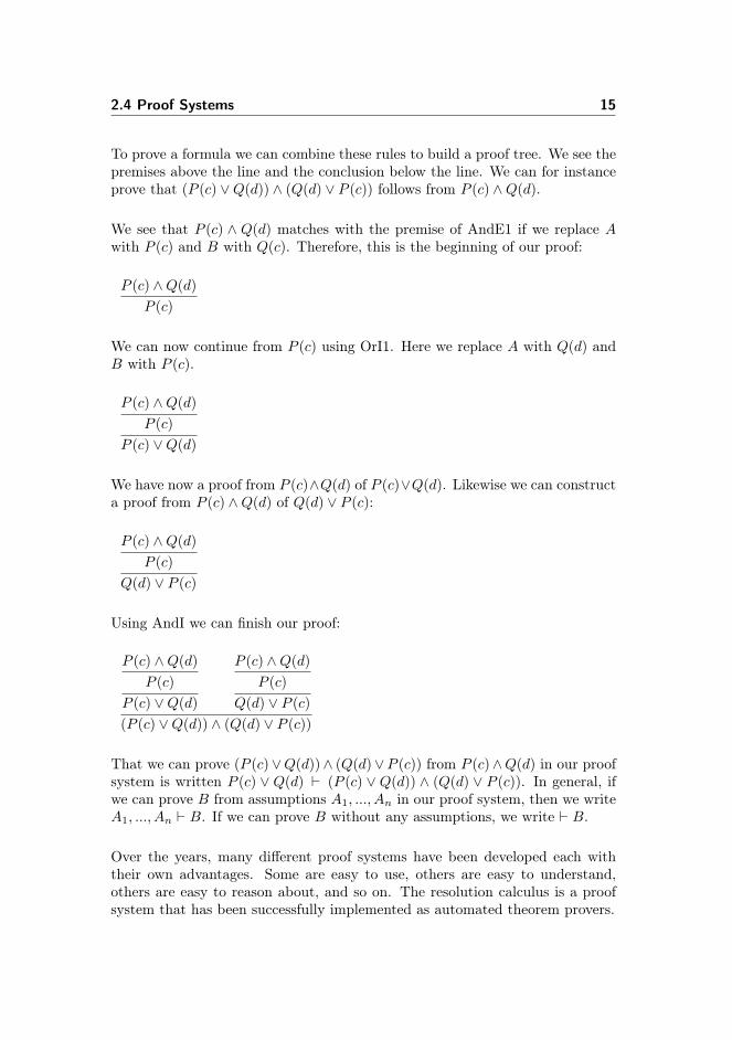
To prove a formula we can combine these rules to build a proof tree. We see thepremises above the line and the conclusion below the line. We can for instanceprove that (P (c) ∨Q(d)) ∧ (Q(d) ∨ P (c)) follows from P (c) ∧Q(d).
We see that P (c) ∧ Q(d) matches with the premise of AndE1 if we replace Awith P (c) and B with Q(c). Therefore, this is the beginning of our proof:
P (c) ∧Q(d)
P (c)
We can now continue from P (c) using OrI1. Here we replace A with Q(d) andB with P (c).
P (c) ∧Q(d)
P (c)
P (c) ∨Q(d)
We have now a proof from P (c)∧Q(d) of P (c)∨Q(d). Likewise we can constructa proof from P (c) ∧Q(d) of Q(d) ∨ P (c):
P (c) ∧Q(d)
P (c)
Q(d) ∨ P (c)
Using AndI we can finish our proof:
P (c) ∧Q(d)
P (c)
P (c) ∨Q(d)
P (c) ∧Q(d)
P (c)
Q(d) ∨ P (c)(P (c) ∨Q(d)) ∧ (Q(d) ∨ P (c))
That we can prove (P (c)∨Q(d))∧ (Q(d)∨P (c)) from P (c)∧Q(d) in our proofsystem is written P (c) ∨ Q(d) ` (P (c) ∨ Q(d)) ∧ (Q(d) ∨ P (c)). In general, ifwe can prove B from assumptions A1, ..., An in our proof system, then we writeA1, ..., An ` B. If we can prove B without any assumptions, we write ` B.
Over the years, many different proof systems have been developed each withtheir own advantages. Some are easy to use, others are easy to understand,others are easy to reason about, and so on. The resolution calculus is a proofsystem that has been successfully implemented as automated theorem provers.
16 Preliminaries and Theory Background
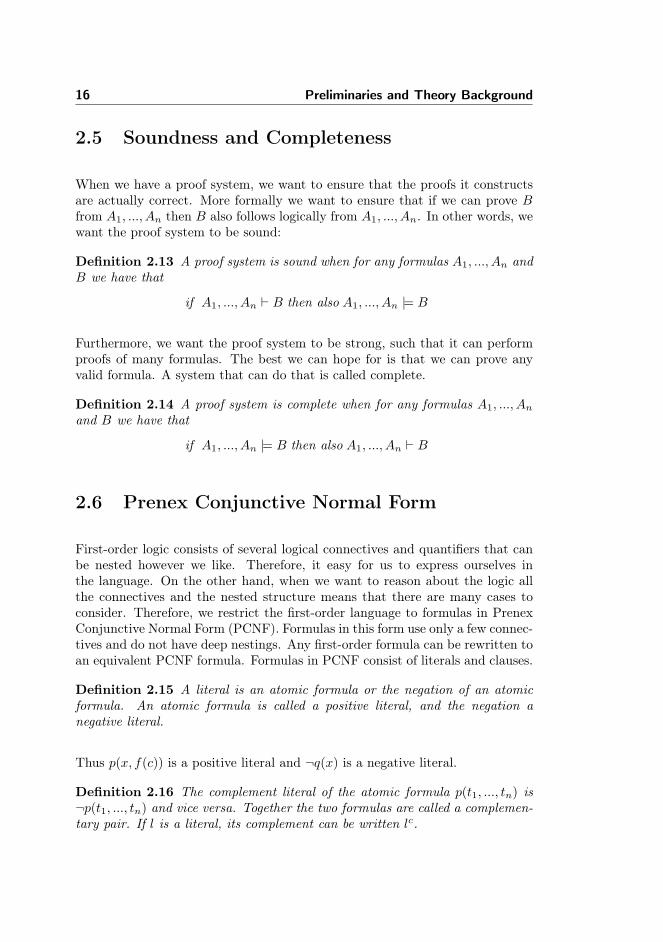
2.5 Soundness and Completeness
When we have a proof system, we want to ensure that the proofs it constructsare actually correct. More formally we want to ensure that if we can prove Bfrom A1, ..., An then B also follows logically from A1, ..., An. In other words, wewant the proof system to be sound:
Definition 2.13 A proof system is sound when for any formulas A1, ..., An andB we have that
if A1, ..., An ` B then also A1, ..., An |= B
Furthermore, we want the proof system to be strong, such that it can performproofs of many formulas. The best we can hope for is that we can prove anyvalid formula. A system that can do that is called complete.
Definition 2.14 A proof system is complete when for any formulas A1, ..., An
and B we have that
if A1, ..., An |= B then also A1, ..., An ` B
2.6 Prenex Conjunctive Normal Form
First-order logic consists of several logical connectives and quantifiers that canbe nested however we like. Therefore, it easy for us to express ourselves inthe language. On the other hand, when we want to reason about the logic allthe connectives and the nested structure means that there are many cases toconsider. Therefore, we restrict the first-order language to formulas in PrenexConjunctive Normal Form (PCNF). Formulas in this form use only a few connec-tives and do not have deep nestings. Any first-order formula can be rewritten toan equivalent PCNF formula. Formulas in PCNF consist of literals and clauses.
Definition 2.15 A literal is an atomic formula or the negation of an atomicformula. An atomic formula is called a positive literal, and the negation anegative literal.
Thus p(x, f(c)) is a positive literal and ¬q(x) is a negative literal.
Definition 2.16 The complement literal of the atomic formula p(t1, ..., tn) is¬p(t1, ..., tn) and vice versa. Together the two formulas are called a complemen-tary pair. If l is a literal, its complement can be written lc.

2.7 Clausal Forms 17
Therefore, p(x, f(c)) is the complement of ¬p(x, f(c)), and vice versa
Definition 2.17 A formula is said to be in Conjunctive Normal Form if it isa conjunction of disjunctions of literals.
Thus, the following is a CNF:
(p(f(x, y), c)) ∨ q(g(c))) ∧ ¬q(f(y))
Definition 2.18 A formula is said to be in Prenex Conjunctive Normal Form,if it has the form
Q1 x1. . . . Qn xn. M
where Q1 . . . Qn each are either ∀ or ∃ and M is in Conjunctive Normal Form.
The resolution calculus additionally requires that Q1 ... Qn all are ∀. Anyformula in first-order logic can be rewritten to an equisatisfiable formula inPCNF where Q1 ... Qn all are ∀.
For instance, the formula
((∀x. p(x)→ q(x)) ∧ (∀y. p(y)))→ ∀z. q(z)
has the equivalent PNCF formula
∃x. ∃y. ∀z. (p(x) ∨ ¬p(y) ∨ q(z)) ∧ (¬q(x) ∨ ¬p(y) ∨ q(z)))
and the equisatisfiable PCNF formula
∀z. (p(a) ∨ ¬p(b) ∨ q(z)) ∧ (¬q(a) ∨ ¬p(b) ∨ q(z))
with only universal quantifiers.
2.7 Clausal Forms
To make it simpler for us to manipulate the formulas, we prefer to representthem as sets. To do this we take a formula ∀x1. ... ∀xn. M where M is in CNFand let each of the disjunctions in F be represented by the set of literals ofwhich it consists.
Definition 2.19 A clause is a set of literals. It represents the disjunction ofthese literals.
18 Preliminaries and Theory Background
Since a clause represents a disjunction, it is satisfied by an interpretation if forany variable denotation some literal in the clause is satisfied. A special case isthe empty clause {}. By this definition it is always false, i.e., it is unsatisfiable,and so represents a contradiction.
We can then collect all the clauses of M in a set of clauses.
Definition 2.20 A clausal form is a disjunction of clauses. It represents theconjunction of those clauses.
For instance (p(f(x, y), c))∨ q(g(c)))∧¬q(f(Y )) becomes {p(f(x, y), c), q(g(c))}and {q(g(c))}, and so the corresponding set of clauses turns out to be the set{{p(f(x, y), c), q(g(c))}, {q(g(c))}}. It is implicit that all the clauses are univer-sally quantified.
2.8 Substitutions
Another important notion in resolution is substitution.
Definition 2.21 A substitution σ is a map from variables to terms.
To apply a substitution σ to a term t, we simultaneously replace each occurrenceof any variable x with σ(x). The result is written t{σ}. This notation is abit different from the literature, which does not use the curly brackets and justwrites tσ. We choose this alternative notation because it looks somewhat similarand can be formalized in Isabelle. Another alternative would be to use · or someother infix operator.
For instance if σ = {x 7→ f(c), y 7→ g(x, y)} and t = f(x, y) then t{σ} =f(f(c), f(x, y)).
Definition 2.22 t is an instance of t′ if there exists some substitution σ suchthat t = t′σ.
For example f(f(c), f(x, y)) is an instance of f(x, y).
Applying substitutions to literals, clauses and sets of clauses is completely anal-ogously defined. We can also define substitution for formulas, but then we onlyreplace variables that are not bound.
2.9 Resolution 19
Substitutions can also be composed.
Definition 2.23 The composition σ·θ of one substitution σ and another θ is thesubstitution that first applies σ to a variable and then applies θ to the resultingterm: (θ · σ)(x) = (σ(x)){θ}
Unifiers are a central concept of resolution:
Definition 2.24 A unifier for a set of terms is a substitution that makes allthe terms equal to each other.
The definition for literals, clauses and sets of clauses is completely analogous.
Most general unifiers is another central concept:
Definition 2.25 A most general unifier (mgu) σ for a set ts of terms is aunifier from which we can construct any other unifier for ts, by compositionwith some other substitution.
In other words, let us say σ is an mgu of the set ts. Then for any unifier θ ofts there exists a substitution s such that σ · s = θ.
The definition for literals, clauses and sets of clauses is completely analogous.
2.9 Resolution
We are now ready to explain the resolution calculus. There are many variantsof this proof system, but they are all based on the following simple rule:
C1 ∨ l C2 ∨ ¬lC1 ∨ C2
The idea of the rule is that we know that l is either true or false. In the firstcase we can from C2 ∨¬l conclude C2 and thus also C1 ∨C2. In the second casewe can from C1 ∨ l conclude that C1 and thus also C1 ∨ C2. So in either casewe can conclude C1 ∨ C2.
We now switch from writing the rule with logical formulas to writing it in theset notation of clauses that we saw in the previous section. While the notation is
20 Preliminaries and Theory Background
not as easily readable as that of formulas, it gives us the freedom to manipulatethe clauses with the mathematical set operators. The simple resolution rule cannow be written
C1 C2
(C1 − {l1}) ∪ (C2 − {l2})
l1 ∈ C1
l2 ∈ C2
l1 = lc2
In first-order logic, we also need rules that take into consideration the variablesand terms. A simple rule that does this is the binary resolution rule.
C1 C2
(C1{σ} − {l1{σ}}) ∪ (C2{σ} − {l2{σ}})
C1 and C2 share no variables,l1 ∈ C1, l2 ∈ C2,σ is an mgu for {l1, lc2}
The rule mirrors the simple resolution rule. The main difference is that l1 andlc2 are unified with the mgu σ which is also applied to the clauses C1 and C2
when the unified literal is removed.
We need to take three steps to get from this rule to a complete proof system forfirst-order logic. The first step is to remedy the problem that the rule requiresthat the two clauses have no variables in common. We fix this by allowing thecalculus to rename the variables of clauses such that they have no variablesin common. This is called standardizing apart. The second step is to remedythe problem that we can only do unification of a complementary pair with oneliteral in each clause. It turns out that it is sometimes necessary to unify wholesets of literals. In chapter 3, we analyze two ways of doing this. The third stepis to use the resolution calculus as a refutation proof system. This means thatwe prove the validity of a formula by proving that its negation is unsatisfiable.Since the negation is false under all interpretations, the formula must be trueunder all interpretations, i.e. valid. The procedure to prove a formula F validis:
1. Negate F to get ¬F .
2. Rewrite ¬F to the equisatisfiable set of clauses cs.
3. Use the rules of a sound resolution calculus to prove the empty clause {}from cs.

2.9 Resolution 21
{} is unsatisfiable. Since the resolution calculus is sound, we get from 3. thatalso cs must be unsatisfiable. Since cs and ¬F are both equisatisfiable, also ¬Fmust be unsatisfiable. Then F must be valid.
Let us try to prove (¬P (c) ∧ ¬Q(d)) ∨Q(d) ∨ (P (c) ∧ ¬Q(d))
As described above we negate the formula: ¬((¬P (c)∧¬Q(d))∨Q(d)∨ (P (c)∧¬Q(d))), and then we turn it into an equisatisfiable set of clauses, so that we canuse the resolution procedure. The set is: {{P (c), Q(d)}, {¬Q(d)}, {¬P (c), Q(d)}}.We can now construct a proof tree:
{P (c), Q(d)} {¬Q(d)}{P (c)}
{¬P (c), Q(d)} {¬Q(d)}{¬P (c)}
{}
In this example, the mgu we used was the empty substitution.
Another way of writing a resolution proof is to write it as a derivation. Aderivation is a sequence cs1, ..., csn of clausal forms where the step from oneclausal csi form to the next csi+1 in the sequence is performed by adding theresolvent of two clauses of csi. We can write such a derivation as a number oflines. The first cs1 lines consist of the clauses of the initial clausal form. Thenext lines are then the clauses that were added by performing the steps. Theproof tree we saw before is presented as a derivation here:
1. {¬P (c), Q(d)}
2. {¬Q(d)}
3. {P (c), Q(d)}
4. {¬P (c)}
5. {P (c)}
6. {}
Since we are using the resolution calculus as a refutation proof system, we arenow actually proving sets of clauses unsatisfiable. Therefore, we can define asuitable notation of completeness.
Definition 2.26 (Refutational Completeness)If the set of clauses cs is unsatisfiable then we can prove the empty clause fromcs, i.e. cs ` {}

22 Preliminaries and Theory Background
2.10 Isabelle
Isabelle is a proof assistant. A proof assistant is a computer program thatcan help its user in conducting proofs of theorems in mathematics, logic andcomputer science. For instance, Isabelle has been used to prove Pythagoras’theorem [Cha15], to prove Gödel’s incompleteness theorems [Pau13], to verifyan operating system kernel [KEH+09] and to prove Dijkstra’s algorithm correct[NL12].
To write a proof in Isabelle the user writes it in a language called Isar. Isar issimilar to English and is thus readable by human beings, but it is also readableby Isabelle. Therefore, Isabelle can help its user in several ways. Most impor-tantly, it checks that the proof is correct, and can even conduct parts of theproof automatically. Isabelle checks the correctness by using a logic. The mostpopular logic for Isabelle is called higher-order logic (HOL).
Figure 2.1: Isabelle/jEdit in action.

2.11 HOL 23
2.11 HOL
Higher-order logic is the logic used by several proof assistants, including Isabelle.HOL can be seen as a combination of functional programming and logic, becauseit contains concepts from both worlds.
From functional programming, HOL gets its recursive functions, lambda func-tions, higher-order functions, pattern matching, and more. HOL also has a typesystem similar to those known from typed functional languages such as F#,Haskell, and Standard ML. From now on, we use the word function instead ofmap, following the terminology of functional programming instead of that ofmathematics. In HOL, a predicate is simply a function with return type bool.
From logic, HOL gets its logical connectives, terms, variables, quantifiers etc.They are similar to those we have seen for first-order logic. A key differencebetween HOL and FOL is that in HOL we can also quantify over functions,predicates and sets of individuals instead of just over individuals as in FOL.

24 Preliminaries and Theory Background
Chapter 3
Analysis of the Problem
There are several variants of the resolution calculus, and several different ap-proaches to proving its soundness and completeness.
This chapter analyzes several different variants of the resolution calculus fromthe literature. It looks at some different completeness proofs, and analyzes howwell suited they are for a formalization. It concludes on which ideas I will basemy formalization.
3.1 Resolution Calculus in the Literature
The variation between different resolution calculi is not only in the notationused to write the system, but also in which rules are in the system. Fittingpresents three different resolution calculi that we will consider here [Fit96].
3.1.1 Binary Resolution with Factoring
We have already seen the binary resolution rule. This rule is usually used to-gether with another rule, called the factoring rule, to form binary resolution with

26 Analysis of the Problem
factoring. We repeat the definition of the binary resolution rule, and introducethe factoring rule.
Definition 3.1 (Binary Resolution Rule)
C1 C2
(C1{σ} − {l1{σ}}) ∪ (C2{σ} − {l2{σ}})
C1 and C2 share no variables,l1 ∈ C1, l2 ∈ C2,σ is an mgu for {l1, lc2}
Definition 3.2 (Factoring Rule)
CC{σ}
σ is an mgu for L ⊆ C
In some presentations the two rules can be used together in any order to con-struct proofs. Another way to define resolution is to let the resolvent be thebinary resolvent of the factors of two clauses.
An advantage of this system is that there are two rules, each of which servetheir own purpose. The factoring rule lets us unify any subset of a clause, andthe resolution rule lets us resolve clauses, such that we can eventually derivethe empty clause. Splitting these functions in to two rules arguably makes thepresentation simpler.
3.1.2 General Resolution
General resolution is another resolution calculus1.
Definition 3.3 (General Resolution Rule)
C1 C2
(C1{σ} − L1{σ}) ∪ (C2{σ} − L2{σ})
C1 and C2 have no variables in common,L1 ⊆ C1, L2 ⊆ C2,σ mgu for L1 ∪ Lc
2
This rule looks very similar to the binary resolution rule, but notice that L1
and L2 are no longer literals, but subsets of literals in C1 and C2 respectively.Therefore, we can see the general resolution rule as a combination of factoringand binary resolution. The difference is that the factoring rule allowed us to dounification of any subset of literals, while the binary resolution rule only allowsunification of the literals that we remove.
1Fitting actually calls it the General Literal Resolution Rule.

3.2 Soundness and Completeness Proofs 27
This resolution calculus is appealing because it consists only of one rule. Thismeans that one is never in doubt about which rule to use when doing resolutionproof, one only has to worry about choosing the right instantiation.
3.1.3 Resolution Suited for Hand Calculation
Fitting introduces a resolution that is suited for hand calculation.2 The reso-lution is quite different from the others. Instead of having a preprocessing stepwhere formulas are rewritten to clauses, the system works directly on formulas,but contains rules that, when applied break the formulas down to clauses. Fur-thermore, this system does not use most general unifiers. Instead, it requiresus to guess with which terms the variables must be substituted. Therefore, thesystem is not well suited as the basis of an automatic theorem prover. For thisreason, Fitting shows how it can be modified to be the general resolution orbinary resolution.
3.1.4 Other Variants of the Resolution Calculus
We have now seen three variants of the resolution calculus. However, one caneven find variants of these variants. For instance, some resolution systems applythe mgu after the literals have been removed.
There are also variants that change or restrict the rules considerably such asordered resolution. The idea is to make the search space smaller by restrictingwhen the resolution rule can be applied [GLJ13]. Furthermore, superposition isan extension of the resolution calculus, that also restricts the search space, anddoes equational reasoning [KNV+13].
3.2 Soundness and Completeness Proofs
We can prove soundness by showing that if the premises of any rule in the systemare satisfied by an interpretation then so is the conclusion. Then the rules allpreserve satisfiability and therefore the whole system must do the same. Thiscan be proven by induction. As such, the overall strategy of a soundness proof
2In the book this is just called first-order resolution, but that name describes all thepresented resolution calculi.

28 Analysis of the Problem
is simple and clear, and therefore the challenge lies in the details of the proofand its formalization.
It is more complicated to prove completeness because here the overall strategyis less clear. For any unsatisfiable clausal form we need to combine rule appli-cations in some way to get a derivation of the empty clause. There are severalapproaches to this. This section explains three different approaches. It does notgo in to all details, but explains the overall ideas thoroughly.
3.2.1 Semantic Trees
The approach used in among others Ben-Ari [BA12] and Chang and Lee [CL73]is semantic trees. We introduce an enumeration A0, A1, A2, . . . of atomic groundformulas i.e. an infinite sequence that contains all atomic formulas that do notcontain variables. The enumeration could for instance be a(), b(), a(a()), . . . .For a given clausal form, the enumeration is restricted to the atoms that can bebuilt from the function and predicate symbols that occur in the clausal form.
a()
b()
a(a())
... ...
¬a(a())
... ...
¬b()
a(a())
... ...
¬a(a())
... ...
¬a()
b()
a(a())
... ...
¬a(a())
... ...
¬b()
a(a())
... ...
¬a(a())
... ...
Figure 3.1: A semantic tree.
3.2.1.1 Definition
A semantic tree is a possibly infinite binary tree in which all nodes are labeledwith a literal. Each level corresponds to an atomic formula. More precisely, on
3.2 Soundness and Completeness Proofs 29
the i’th level, all literals are either Ai or its negation. When we go left in abranching of the tree we come to an atom, and when we go right, we come tothe negation of an atom. More precisely all left children are positive literals andall right children are negative literals. To sum up, the left children on level i ofthe tree are labeled with atomic formula Ai and the right children on level i arelabeled with its negation ¬Ai. Figure 3.1 shows a semantic tree.
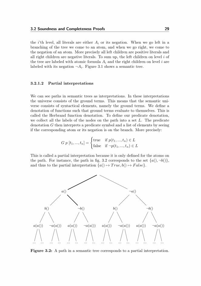
3.2.1.2 Partial interpretations
We can see paths in semantic trees as interpretations. In these interpretationsthe universe consists of the ground terms. This means that the semantic uni-verse consists of syntactical elements, namely the ground terms. We define adenotation of functions such that ground terms evaluate to themselves. This iscalled the Herbrand function denotation. To define our predicate denotation,we collect all the labels of the nodes on the path into a set L. The predicatedenotation G then interprets a predicate symbol and a list of elements by seeingif the corresponding atom or its negation is on the branch. More precisely:
G p [t1, ..., tn] =
{true if p(t1, ..., tn) ∈ Lfalse if ¬p(t1, ..., tn) ∈ L
This is called a partial interpretation because it is only defined for the atoms onthe path. For instance, the path in fig. 3.2 corresponds to the set {a(),¬b()},and thus to the partial interpretation {a() 7→ True, b() 7→ False}.
a()
b()
a(a())
... ...
¬a(a())
... ...
¬b()
a(a())
... ...
¬a(a())
... ...
¬a()
b()
a(a())
... ...
¬a(a())
... ...
¬b()
a(a())
... ...
¬a(a())
... ...
Figure 3.2: A path in a semantic tree corresponds to a partial interpretation.
30 Analysis of the Problem
3.2.1.3 Herbrand’s Lemma and Closed Semantic Trees
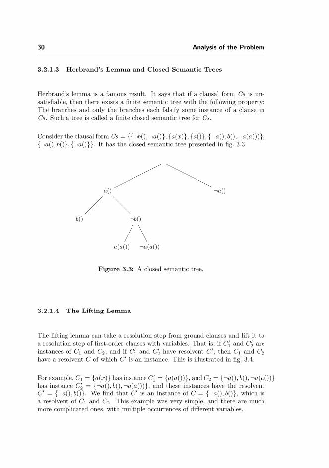
Herbrand’s lemma is a famous result. It says that if a clausal form Cs is un-satisfiable, then there exists a finite semantic tree with the following property:The branches and only the branches each falsify some instance of a clause inCs. Such a tree is called a finite closed semantic tree for Cs.
Consider the clausal form Cs = {{¬b(),¬a()}, {a(x)}, {a()}, {¬a(), b(),¬a(a())},{¬a(), b()}, {¬a()}}. It has the closed semantic tree presented in fig. 3.3.
a()
b() ¬b()
a(a()) ¬a(a())
¬a()
Figure 3.3: A closed semantic tree.
3.2.1.4 The Lifting Lemma
The lifting lemma can take a resolution step from ground clauses and lift it toa resolution step of first-order clauses with variables. That is, if C ′1 and C ′2 areinstances of C1 and C2, and if C ′1 and C ′2 have resolvent C ′, then C1 and C2
have a resolvent C of which C ′ is an instance. This is illustrated in fig. 3.4.
For example, C1 = {a(x)} has instance C ′1 = {a(a())}, and C2 = {¬a(), b(),¬a(a())}has instance C ′2 = {¬a(), b(),¬a(a())}, and these instances have the resolventC ′ = {¬a(), b()}. We find that C ′ is an instance of C = {¬a(), b()}, which isa resolvent of C1 and C2. This example was very simple, and there are muchmore complicated ones, with multiple occurrences of different variables.

3.2 Soundness and Completeness Proofs 31
resolution
instance
ground
C2C1
C ′1 C ′2
C ′
C
Figure 3.4: The lifting lemma.
3.2.1.5 Completeness
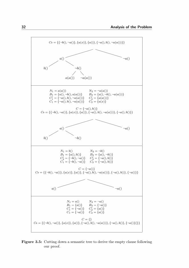
We now have the tools needed to prove completeness. Therefore, we consider anunsatisfiable clausal form Cs. We use Herbrand’s lemma to construct a finiteclosed semantic tree. Next, we find a node N in the tree whose children are twobranch nodes and call their labels A and ¬A respectively. We let their pathsto the root be B, B1 = B ∪ {A}, and B2 = B ∪ {¬A}, respectively. Since B isnot a branch of the closed semantic tree, it does not falsify a clause. But sinceB ∪ {A} is a branch, it must falsify some instance C ′1 of a clause C1 in Cs. Itmust have been making the union of {A} and B that made all the literals inC ′1 false, and thus C ′1 must contain ¬A, and all its other literals were alreadyfalsified by B. The same is true for B2 and a corresponding C ′2 and C2. If welook at the resolvent C ′ = (C ′1 − {¬A}) ∪ (C ′2 − {A}) of C ′1 and C ′2, then wesee that it contains literals that are all falsified by B, because we removed thetwo that were not. Using the lifting lemma, can resolve C1 and C2 to get aresolvent C which has instance C ′. If we remove N1 and N2 from the tree, butadd C to Cs, then the modified tree is a closed semantic tree for the modifiedCs, because B falsifies C ′ which is an instance of C, and all other branches arealready closed.
We can keep doing this until the tree is cut down completely. It turns out thatin this last step, the empty clause is derived. Thus, we have shown that for theunsatisfiable set of clauses indeed we can derive the empty clause.
We perform this process for our example in fig. 3.5.
32 Analysis of the Problem
Cs = {{¬b(),¬a()}, {a(x)}, {a()}, {¬a(), b(),¬a(a())}}
a()
b() ¬b()
a(a()) ¬a(a())
¬a()
N1 = a(a()) N2 = ¬a(a())B1 = {a(),¬b(), a(a())} B2 = {a(),¬b(),¬a(a())}C′1 = {¬a(), b(),¬a(a())} C′2 = {a(a())}C1 = {¬a(), b(),¬a(a())} C2 = {a(x)}
C = {¬a(), b()}Cs = {{¬b(),¬a()}, {a(x)}, {a()}, {¬a(), b(),¬a(a())}, {¬a(), b()}}
a()
b() ¬b()
¬a()
N1 = b() N2 = ¬b()B1 = {a(), b()} B2 = {a(),¬b()}C′2 = {¬b(),¬a()} C′2 = {¬a(), b()}C1 = {¬b(),¬a()} C2 = {¬a(), b()}
C = {¬a()}Cs = {{¬b(),¬a()}, {a(x)}, {a()}, {¬a(), b(),¬a(a())}, {¬a(), b()}, {¬a()}}
a() ¬a()
N1 = a() N2 = ¬a()B1 = {a()} B2 = {¬a()}C′1 = {¬a()} C′2 = {a()}C1 = {¬a()} C2 = {a()}
C = {}Cs = {{¬b(),¬a()}, {a(x)}, {a()}, {¬a(), b(),¬a(a())}, {¬a(), b()}, {¬a()}{}}
Figure 3.5: Cutting down a semantic tree to derive the empty clause followingour proof.
3.2 Soundness and Completeness Proofs 33
3.2.1.6 Thoughts on the proof
This proof is in many ways very intuitive, because it uses trees, which are knownfrom many different areas of informatics. Furthermore, the trees give us a verysimple and graphical way to think about the interpretations, and we can applyresults from graph theory. Completeness is a statement about interpretations,and they are represented directly in the semantic tree. Lastly, the presentationof semantic trees by Chang and Lee [CL73] is quite thorough, and goes in tomany details, which can help make the formalization process go smoothly.
3.2.2 Consistency Properties
As said, Fitting [Fit96] introduces a resolution suited for hand calculation. Toprove its completeness, he uses the following reformulation of completeness:
Property 1 If ⊥ cannot be proven from a set of formulas S, then S has amodel.
Therefore, he considers any set of formulas S from which ⊥ cannot be derived.He then proves that S is a member of what he calls a consistency property. Thefamous “Model Existence Theorem” tells us that any member of a consistencyproperty is satisfiable.
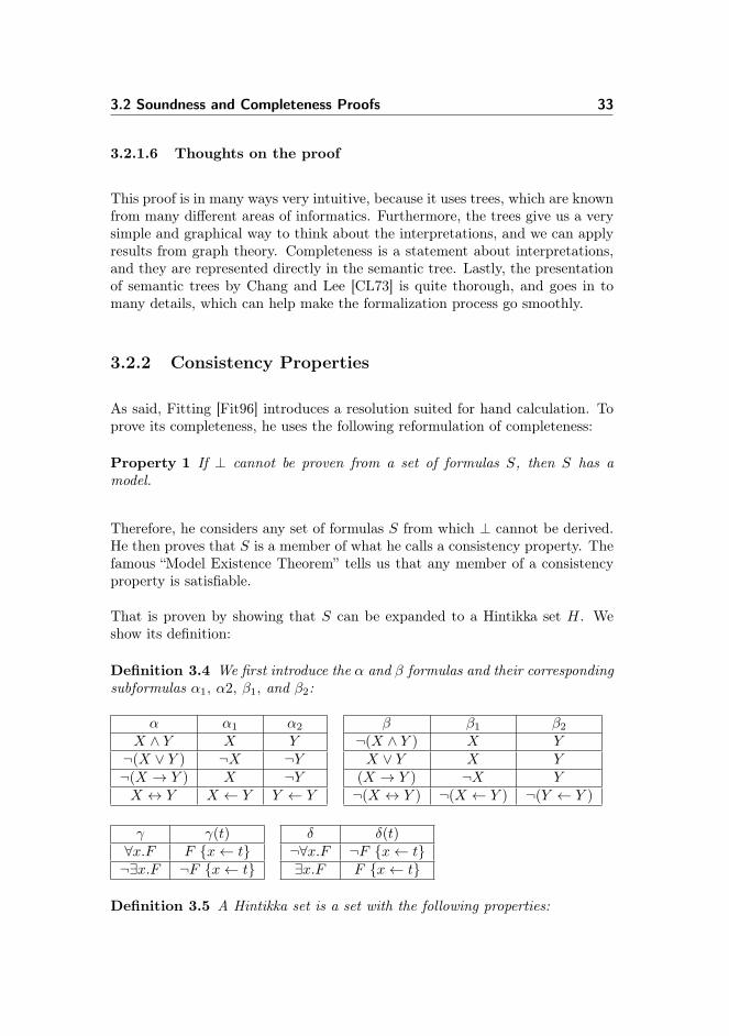
That is proven by showing that S can be expanded to a Hintikka set H. Weshow its definition:
Definition 3.4 We first introduce the α and β formulas and their correspondingsubformulas α1, α2, β1, and β2:
α α1 α2
X ∧ Y X Y¬(X ∨ Y ) ¬X ¬Y¬(X → Y ) X ¬YX ↔ Y X ← Y Y ← Y
β β1 β2¬(X ∧ Y ) X YX ∨ Y X Y
(X → Y ) ¬X Y¬(X ↔ Y ) ¬(X ← Y ) ¬(Y ← Y )
γ γ(t)∀x.F F {x← t}¬∃x.F ¬F {x← t}
δ δ(t)¬∀x.F ¬F {x← t}∃x.F F {x← t}
Definition 3.5 A Hintikka set is a set with the following properties:

34 Analysis of the Problem
1. H does not contain both an atomic formula A and its negation ¬A.
2a. H does not contain ⊥.
2b. H does not contain ¬>.
3. If H contains a double negation ¬¬Z of a formula then H also containsZ.
4. If H contains an alpha formula α then H also contains α1 and α2.
5. If H contains a beta formula β then H also contain β1 or β2.
6. If H contains a gamma formula γ then H contains γ(t) for every closedterm t of the language.
7. If H contains a delta formula δ then H contains γ(t) for some closed termof the language.
Then it is shown that any Hintikka set has a model. The model uses the Her-brand function denotation and the predicate denotation G is then defined:
G P [t1, ..., tn] =
{true if P (t1, ..., tn) ∈ Hfalse otherwise
It is then easy to show that this interpretation satisfies H, and thus also thesubset S. The proof is by induction. Fitting also shows how to lift the proof togeneral resolution and binary resolution with factoring using a lifting lemma.
The main appeal of this approach is that a lot of the formalization work hasbeen done beforehand. Berghofer’s formalization in Isabelle of a natural de-duction proof system [Ber07] uses the framework of consistency properties toprove soundness and completeness. Therefore, one could formalize the resolu-tion system from Fittings book and prove it complete by applying the lemmasformalized by Berghofer. The challenging part would be to extend the proof towork for also general resolution or binary resolution with factoring.
3.2.3 Unified Completeness
A third approach is presented in Blanchette, Popescu, and Traytel’s complete-ness proof for a Genzen proof system [BPT14b].
3.2 Soundness and Completeness Proofs 35
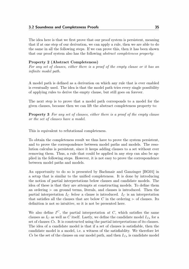
The idea here is that we first prove that our proof system is persistent, meaningthat if at one step of our derivation, we can apply a rule, then we are able to dothe same in all the following steps. If we can prove this, then it has been shownthat our proof system also has the following abstract completeness property :
Property 2 (Abstract Completeness)For any set of clauses, either there is a proof of the empty clause or it has aninfinite model path.
A model path is defined as a derivation on which any rule that is ever enabledis eventually used. The idea is that the model path tries every single possibilityof applying rules to derive the empty clause, but still goes on forever.
The next step is to prove that a model path corresponds to a model for thegiven clauses, because then we can lift the abstract completeness property to:
Property 3 For any set of clauses, either there is a proof of the empty clauseor the set of clauses have a model.
This is equivalent to refutational completeness.
To obtain the completeness result we thus have to prove the system persistent,and to prove the correspondence between model paths and models. The reso-lution calculus is persistent, since it keeps adding clauses to a set without everremoving them. Thus, a rule that could be applied in any step can also be ap-plied in the following steps. However, it is not easy to prove the correspondencebetween model paths and models.
An opportunity to do so is presented by Bachmair and Ganzinger [BG01] ina setup that is similar to the unified completeness. It is done by introducingthe notion of partial interpretations below clauses and candidate models. Theidea of these is that they are attempts at constructing models. To define theman ordering � on ground terms, literals, and clauses is introduced. Then thepartial interpretation IC below a clause is introduced. IC is an interpretationthat satisfies all the clauses that are below C in the ordering � of clauses. Itsdefinition is not so intuitive, so it is not be presented here.
We also define IC , the partial interpretation at C, which satisfies the sameclauses as IC as well as C itself. Lastly, we define the candidate model ICs for aset of clauses Cs. It is constructed using the partial interpretations of its clauses.The idea of a candidate model is that if a set of clauses is satisfiable, then thecandidate model is a model, i.e. a witness of the satisfiablity. We therefore letCs be the set of the clauses on our model path, and then ICs is candidate model
36 Analysis of the Problem
for Cs. We now define a counter-example to be a clause in Cs that is falsifiedby ICs . It is proven that if Cs were to contain a counter-example, then it wouldalso contain the empty clause. The argument is that then the empty clausecould be derived using the counter-example, and since the model path takesevery opportunity to derive things, it would indeed be derived. However, themodel path does by definition not contain the empty clause (since then it wouldnot be infinite), and thus it cannot contain a counter-example. Therefore, ICs
satisfies all clauses and is thus a model.
Bachmair and Ganzinger shows this result for a proof system called ground res-olution, but also indicate how this result can be lifted to the resolution calculusfor first-order logic using a lemma called the lifting lemma.
The unified completeness comes with a formalization in Isabelle [BPT14a].Therefore, like the consistency properties, this approach is appealing, becausesome of the work is already done. Furthermore, it is quite elegant that we takethe infinite derivation and from that build a model more or less directly. Assaid, it should be easy to prove resolution persistent. However, we still needto make a formalization of the candidate models. This could prove to be dif-ficult, because the ordering on formulas is not very intuitive. Additionally, wehave to find out how to lift the result from ground resolution to a resolution forfirst-order logic.
3.3 Other Considerations
For a resolution prover to be useful, we need to implement an algorithm totranslate formulas of the first-order logic to clauses. This is useful because thenwe are be able to prove formulas correct. Most, if not all, resolution basedautomatic theorem provers include such machinery, and it is a challenge in itselfto write an efficient rewriting algorithm.
To make an automatic theorem prover, we need to find a way to make the proofsystem executable. It is possible to extract Standard ML code from an Isabelletheory, to get an executable program. This approach has been used to makea verified automatic theorem prover [Rid04]. It does, however, require quitesome work to go from an abstract definition of a proof system to one that isexecutable.
3.4 Other Presentations 37
3.4 Other Presentations
There are several other interesting presentations of the resolution calculus thanthose discussed above. One is by Robinson, the original inventor of the res-olution calculus [Rob79]. Another is a book by Leitsch dedicated entirely toresolution [Lei97]. Furthermore, Bachmair and Ganzinger have written an ad-vanced chapter on resolution [BG01].
3.5 The Approach of This Project
In this project, I have chosen to formalize general resolution. My motivation isthat it is well suited for automation because of its use of most general unifiers.This mean that my formalization eventually could serve as the basis of an au-tomatic theorem prover. Furthermore, a proof of the completeness of this rulecan easily be adapted to a proof of the completeness of binary resolution withfactoring [Fit96].
I have chosen to make a formalization of the completeness using the semantictree approach. My assessment is that this approach is most likely to be suc-cessful. Semantic trees can be drawn as graphs on a paper, which often helpswith intuition. This choice also gives me a better understanding of the processof formalizing completeness, since I cannot cut corners by using the already de-veloped frameworks for consistency properties [Ber07] and unified completeness[BPT14b]. Furthermore, it also makes the project more interesting seen from aresearch perspective, because in this way my project contributes a formalizationof not only resolution but also semantic trees. I mostly base my formalizationof semantic trees on the presentations of Ben-Ari [BA12] and of Chang and Lee[CL73].
Instead of looking at how to rewrite general formulas to clauses and at mak-ing the system into an automatic theorem prover, the focus is on formalizingresolution, soundness and completeness. This in itself is both interesting andchallenging.

38 Analysis of the Problem

Chapter 4
Formalization: LogicalBackground
This chapter formalizes most of the logical background from chapter 2 up toand including substitution. The chapter shows formalized definitions, lemmas,and theorems of the logical background. The chapter introduces concepts fromIsabelle, Isar, and HOL as they are used in the formalization process.
4.1 Terms
We wish to formalize terms. Therefore, we first need to formalize variable sym-bols, function symbols, and predicate symbols. We represent them by strings,introducing the types var-sym, fun-sym, and pred-sym as synonyms for the stringtype.
type-synonym var-sym = stringtype-synonym fun-sym = stringtype-synonym pred-sym = string

40 Formalization: Logical Background
A more abstract approach is to represent them by type variables, which canthen later be instantiated by a concrete type. On paper, strings are, however,almost always used, and a concrete type makes later definitions simpler sincewe do not have to carry the type variables around. Another advantage is thatthe type of strings is countably infinite which means that the strings can beenumerated. Both concrete types [Rid04] and type variables [Ber07] have beenused in other formalizations.
We now formalize the terms of first-order logic as a type fterm. For this pur-pose we use datatypes, which is a well-known concept from typed functionalprogramming.
datatype fterm =Fun fun-sym fterm list| Var var-sym
This mirrors our definition from chapter 2, which stated that a term is either avariable or a function symbol applied to a list of terms.
Here are some examples of terms:
value Var ′′x ′′
value Fun ′′one ′′ []value Fun ′′mul ′′ [Var ′′y ′′,Var ′′y ′′]value Fun ′′add ′′ [Fun ′′mul ′′ [Var ′′y ′′,Var ′′y ′′], Fun ′′one ′′ []]
In the syntax of chapter 2 they respectively correspond to x, one(),mul(y, y),and add(mul(y, y), one()).
Since that chapter described syntax, it was clear that a variable x was differentfrom a function application f(c(), d()) and therefore we did not state it explicitly.Fortunately, datatypes have the same property. Terms made with differentconstructors are by definition also different.
4.2 Literals
We can likewise define literals as a datatype with one constructor Pos for positiveliterals and another Neg for negative literals:
4.2 Literals 41
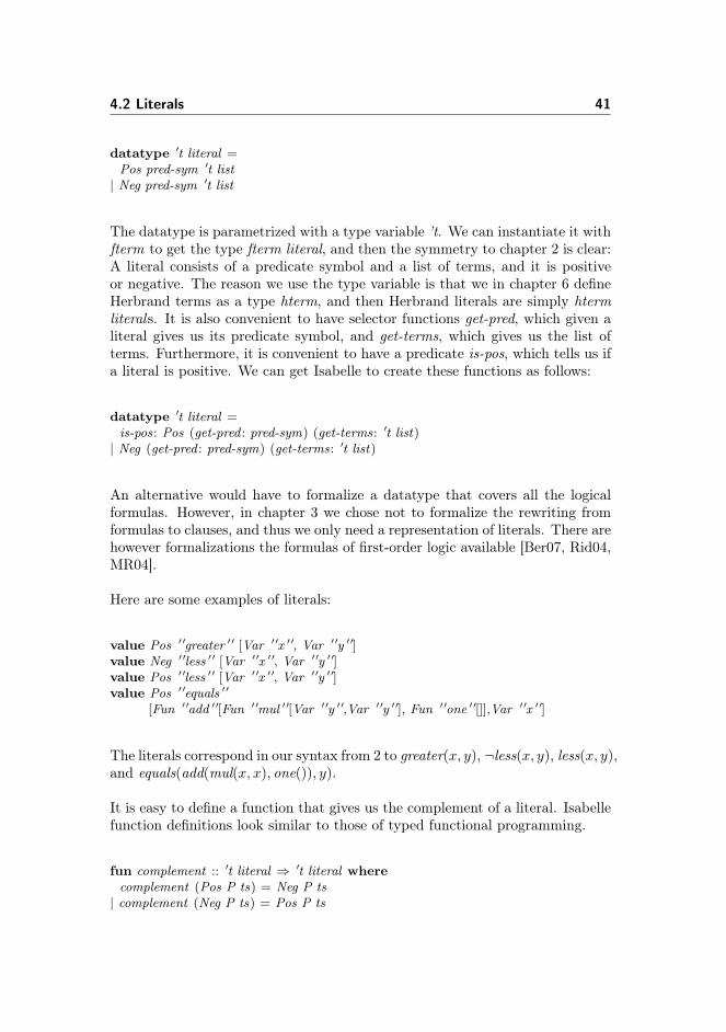
datatype ′t literal =Pos pred-sym ′t list| Neg pred-sym ′t list
The datatype is parametrized with a type variable ’t. We can instantiate it withfterm to get the type fterm literal, and then the symmetry to chapter 2 is clear:A literal consists of a predicate symbol and a list of terms, and it is positiveor negative. The reason we use the type variable is that we in chapter 6 defineHerbrand terms as a type hterm, and then Herbrand literals are simply htermliterals. It is also convenient to have selector functions get-pred, which given aliteral gives us its predicate symbol, and get-terms, which gives us the list ofterms. Furthermore, it is convenient to have a predicate is-pos, which tells us ifa literal is positive. We can get Isabelle to create these functions as follows:
datatype ′t literal =is-pos: Pos (get-pred : pred-sym) (get-terms: ′t list)| Neg (get-pred : pred-sym) (get-terms: ′t list)
An alternative would have to formalize a datatype that covers all the logicalformulas. However, in chapter 3 we chose not to formalize the rewriting fromformulas to clauses, and thus we only need a representation of literals. There arehowever formalizations the formulas of first-order logic available [Ber07, Rid04,MR04].
Here are some examples of literals:
value Pos ′′greater ′′ [Var ′′x ′′, Var ′′y ′′]value Neg ′′less ′′ [Var ′′x ′′, Var ′′y ′′]value Pos ′′less ′′ [Var ′′x ′′, Var ′′y ′′]value Pos ′′equals ′′
[Fun ′′add ′′[Fun ′′mul ′′[Var ′′y ′′,Var ′′y ′′], Fun ′′one ′′[]],Var ′′x ′′]
The literals correspond in our syntax from 2 to greater(x, y), ¬less(x, y), less(x, y),and equals(add(mul(x, x), one()), y).
It is easy to define a function that gives us the complement of a literal. Isabellefunction definitions look similar to those of typed functional programming.
fun complement :: ′t literal ⇒ ′t literal wherecomplement (Pos P ts) = Neg P ts| complement (Neg P ts) = Pos P ts
42 Formalization: Logical Background
We can use a notation similar to that of chapter 2 to make lemmas and theoremseasier to read. Luckily, Isabelle allows us to do that with its mixfix notation.We therefore instead define the complement as:
fun complement :: ′t literal ⇒ ′t literal (-c [300 ] 300 ) where(Pos P ts)c = Neg P ts| (Neg P ts)c = Pos P ts
This allows us to write lc instead of complement l.
If we take the double complement (lc)c of a literal, we obviously get the literall. We prove this small lemma in Isabelle:
lemma cancel-comp1 : (lc)c = l by (cases l) auto
Here, we named the lemma cancel-comp1 and stated it as (lc)c = l. We havemade Isabelle prove it by writing by (cases l) auto. Here (cases l) auto tellsIsabelle how it should conduct the proof. Writing cases l splits the lemma into two cases - one where l is a positive literal and one where it is negative.Then it leaves it up to us to prove the cases separately. We use auto to provethem automatically. Writing auto invokes a proof method that does primarilysimplifications, but also some other forms of reasoning. This concludes the proofin Isabelle.
There are many other proof methods including simp, blast, and metis. Theyeach have their strengths and weaknesses. It is not necessary to know in detailshow they work, but it is an advantage to have an intuition about when touse the different methods. Here is a short explanation of my intuition for thedifferent proof methods. The pure simplification component of auto is simp.It knows about the Isabelle library from a large number of simplification rules.Sometimes the reasoning of auto means that it works itself into a corner, wheresimp instead would have been able to succeed by using only simplification rules.On the other hand, simp sometimes gives up because it does not do the reasoningthat auto does. The proof method blast is efficient at solving problems thatare, in nature, first-order problems. Furthermore, it often chooses the rightinstantiations of the lemmas with which we provide it. The proof method metisis a resolution prover, and is sometimes able to do the proofs where the othermethods give up. Furthermore, Isabelle has a built-in tool called Sledgehammerthat applies automatic theorem provers such as E, SPASS, and Vampire as wellas satisfiability-modulo-theories such as CVC4 and Z3 to prove theorems orstatements automatically [Bla15]. The tool often suggests that we use metistogether with an appropriate set of lemmas.

4.2 Literals 43
We do another proof of a simple property of literals:
lemma cancel-comp2 :assumes asm: l1c = l2c
shows l1 = l2proof −from asm have (l1c)c = (l2c)c by autothen have l1 = (l2c)c using cancel-comp1 [of l1] by autothen show ?thesis using cancel-comp1 [of l2] by auto
qed
This lemma states that assuming l1 c = l2c we have the thesis l1 = l2 . Therefore,
we are proving that if the complements of two literals are the same, then soare the literals. By writing proof, we tell Isabelle that we want to prove thisourselves using however many steps we want or we have to. The "−" tells Isabellethat we want to make a direct proof. Our proof starts from the assumption andshows from it that (l1
c)c = (l2c)c using the auto proof method. From this we
show l1 = (l2c)c by canceling out the two applications of complement on the
left hand side. Writing using cancel-comp1 [of l1] by auto means that we useauto to show this proof line and that it can use the lemma cancel-comp1 [ofl1]. The lemma cancel-comp1 [of l1] is the same as cancel-comp1, except that lis instantiated with l1 . Then we show our thesis using cancel-comp2 [of l2] tocancel out the applications of complement on the right hand side. In Isabellethe thesis automatically gets the short name ?thesis. Writing qed indicates thatthe proof is done.
This style of writing a proof is similar to how one could write a proof in anatural language. Words like from, have, then, using, and show mean (atleast almost) the same as they do in English. In longer Isabelle proofs, thesimilarity to natural language is even clearer.
Another easy proof is that of the existence of a complement
lemma comp-exi1 : ∃ l ′. l ′ = lc by (cases l) auto
Note that ∃ is not the existential quantifier for the first-order logic we considerin the thesis. It is instead the existential quantifier of the HOL of Isabelle. InEnglish we could express the lemma as “any literal has a complement”, but sincewe are writing in the HOL of Isabelle we must use its existential quantifier. Thesame is the case when we see the ∀ quantifier, and the connectives ¬,−→,←→,∨,and ∧. A connective we did not see in first-order logic was =⇒. In Isabelle, this

44 Formalization: Logical Background
arrow separates an assumption from a conclusion. The statements A =⇒ B andA −→ B are logically equivalent. It is often more appropriate to write A =⇒ B,but A −→ B can be nested inside any logical construction. We will not dwellmore on the difference, which can be studied elsewhere [NK14].
It takes a bit more effort to show the following similar lemma:
lemma comp-exi2 : ∃ l . l ′ = lc
proofshow l ′ = (l ′c)c using cancel-comp1 [of l ′] by auto
qed
Again, we tell Isabelle that we want to prove the theorem in some steps, but thistime we do not use the−. This means that Isabelle choses an appropriate rule forus to prove the lemma. Since the lemma is an existential quantification, Isabellechooses the rule P x =⇒ ∃x. P x. The rule says that we can prove ∃x. P x byproving P x for some x. In the proof of comp-exi2 the P x corresponds to(l′ = xc). The x for which we prove it, is l′c.
We also prove
lemma comp-swap: l1c = l2 ←→ l1 = l2c
proof −have l1c = l2 =⇒ l1 = l2c using cancel-comp1 [of l1] by automoreoverhave l1 = l2c =⇒ l1c = l2 using cancel-comp1 by autoultimatelyshow ?thesis by auto
qed
Here we see a new concept, namely the “... moreover ... ultimately” construc-tion. In this construction the last statement before “moreover” and the laststatement before “ultimately” are collected and provided to the application ofauto on the statement following “ultimately”. If we wanted to collect morestatements, we could have used additional “moreover” commands.
4.3 Clauses
We now formalize clauses. Sets are already defined in Isabelle, and so it is easyto define clauses as a synonym for sets of literals:
4.4 Collecting Variables 45
type-synonym ′t clause = ′t literal set
The clauses we consider are always finite, but a set can actually be infinite.Therefore, another possibility would have been to use the type fset of finite sets.Furthermore, some presentations of the resolution calculus use multisets. We usesets because their notation in Isabelle is similar to the well-known mathematicalnotation. The only major difference from mathematical notation is that Isabelleuses a dot instead of the bar when writing for instance the set of all elements witha certain property {x. P (x)}. The proof methods of Isabelle reason efficientlyabout sets.
We extend the concept of complement to sets of literals, i.e. clauses.
abbreviation complementls :: ′t literal set ⇒ ′t literal set (-C [300 ] 300 ) whereLC ≡ complement ‘ L
The superscript C used here is capital. We use abbreviation to define comple-mentls. This seems similar to fun, and is used in much the same way. However,contrary to fun, it does not introduce a function in the logic. Instead Isabelleintroduces complementls L as a syntactical shorthand for complement ‘ L.
The operator ‘ is a higher-order map function. It applies complement to everyliteral in L. In other words, LC is the image of L under the function complement.
4.4 Collecting Variables
In chapter 2 we looked at occurrences of variables and we saw that the generalresolution rule required that its clauses did not share any variables. We thereforecreate functions that collect the variables that occur in terms, lists of terms,literals, and sets of literals. On terms we define it recursively:
fun varst :: fterm ⇒ var-sym setand varsts :: fterm list ⇒ var-sym set wherevarst (Var x ) = {x}| varst (Fun f ts) = varsts ts| varsts [] = {}| varsts (t # ts) = (varst t) ∪ (varsts ts)

46 Formalization: Logical Background
The # is the cons operator with takes element t and puts it at the beginningof list ts. Note that Isabelle functions are required to be be terminating. Formany functions Isabelle can automatically check that this is the case [NK14].
On literals we just look in the term:
definition varsl :: fterm literal ⇒ var-sym set wherevarsl l = varsts (get-terms l)
Here we used definition instead of fun to define a non-recursive function. Incontrary to fun, definition does not add simplification rules to the proof methodsof Isabelle. Therefore, we have to unfold the definition manually when necessary.We can use definition when we want to reason about a function by using itsproperties instead of having Isabelle unfold its definition automatically.
On sets of literals we take the union over the literals in the clause to collecttheir variables:
definition varsls :: fterm literal set ⇒ var-sym set wherevarsls L ≡
⋃l∈L. varsl l
4.5 Ground
A ground term is a term in which no variables occur. As we noted in the analysis,the semantic trees are labeled with ground literals, so this concept must also beformalized. We can easily make a recursive predicate that checks if a term doesnot contains variables:
fun ground :: fterm ⇒ bool whereground (Var x ) ←→ False| ground (Fun f ts) ←→ (∀ t ∈ set ts. ground t)
abbreviation grounds :: fterm list ⇒ bool wheregrounds ts ≡ (∀ t ∈ set ts. ground t)
Since ground and grounds return booleans, we use ←→ in the definition insteadof =. We then extend the definition to literals and sets of literals. For terms,we simply check the list of terms:
4.6 Semantics 47
abbreviation groundl :: fterm literal ⇒ bool wheregroundl l ≡ grounds (get-terms l)
And for sets of literals, we check all the contained literals:
abbreviation groundls :: fterm clause ⇒ bool wheregroundls L ≡ ∀ l ∈ L. groundl l
4.6 Semantics
We are ready to introduce the semantics of terms, literals, and clauses. Firstly,we need to define function denotations, predicate denotations, and variable de-notations:
type-synonym ′u fun-denot = fun-sym ⇒ ′u list ⇒ ′utype-synonym ′u pred-denot = pred-sym ⇒ ′u list ⇒ booltype-synonym ′u var-denot = var-sym ⇒ ′u
Here, we have let the universe be represented by a type variable ′u. This meanthat we are able to use our logic to reason about elements of any type byinstantiating ′u with the desired type.
If we for instance want to reason about the natural numbers, we can instantiate′u with the type nat, and reason about functions and predicates on naturalnumbers. We can do that by defining a nat fun-denot, a nat pred-denot, and anat var-denot.
fun Fnat :: nat fun-denot whereFnat f [n,m] =(if f = ′′add ′′ then n + m elseif f = ′′mul ′′ then n ∗ m else 0 )
| Fnat f [] =(if f = ′′one ′′ then 1 elseif f = ′′zero ′′ then 0 else 0 )
| Fnat f us = 0
fun Gnat :: nat pred-denot whereGnat p [x ,y ] =
48 Formalization: Logical Background
(if p = ′′less ′′ ∧ x < y then True elseif p = ′′greater ′′ ∧ x > y then True elseif p = ′′equals ′′ ∧ x = y then True else False)
| Gnat p us = False
fun Enat :: nat var-denot whereEnat x =
(if x = ′′x ′′ then 26 elseif x = ′′y ′′ then 5 else 0 )
Alternatively, we could have fixed a specific type, or we could have defined anabstract type for the purpose of representing the universe. There are examplesof using a type variable [Ber07] and of using an abstract type [MR04, Rid04] informalizations. We choose to use a type variable, because it allows our logic toreason about anything that can be formalized as a type.
We now formalize the semantics of terms:
fun evalt :: ′u var-denot ⇒ ′u fun-denot ⇒ fterm ⇒ ′u whereevalt E F (Var x ) = E x| evalt E F (Fun f ts) = F f (map (evalt E F ) ts)
We use the higher order function map to apply the function evalt E F to ts, i.e.map (eval E F ) [t1, . . . , tn] = [eval E F t1, . . . , eval E F tn].
As an example we can try to evaluate the terms, function denotations andvariable denotations we used as examples.
lemma evalt Enat Fnat (Var ′′x ′′) = 26by auto
lemma evalt Enat Fnat (Fun ′′one ′′ []) = 1by auto
lemma evalt Enat Fnat (Fun ′′mul ′′ [Var ′′y ′′,Var ′′y ′′]) = 25by auto
lemmaevalt Enat Fnat (Fun ′′add ′′ [Fun ′′mul ′′ [Var ′′y ′′,Var ′′y ′′], Fun ′′one ′′ []]) = 26by auto
We often need to apply the evaluation of terms to lists of terms:
abbreviation evalts :: ′u var-denot ⇒ ′u fun-denot ⇒ fterm list ⇒ ′u list whereevalts E F ts ≡ map (evalt E F ) ts

4.6 Semantics 49
The next step is to evaluate literals. This is done by evaluating the list of terms,and using the predicate denotation to get the meaning of the predicate symbol:
fun evall :: ′u var-denot ⇒ ′u fun-denot ⇒ ′u pred-denot ⇒ fterm literal ⇒ boolwhereevall E F G (Pos p ts) ←→ (G p (evalts E F ts))| evall E F G (Neg p ts) ←→ ¬(G p (evalts E F ts))
We present some examples:
lemma evall Enat Fnat Gnat (Pos ′′greater ′′ [Var ′′x ′′, Var ′′y ′′]) = Trueby auto
lemma evall Enat Fnat Gnat (Neg ′′less ′′ [Var ′′x ′′, Var ′′y ′′]) = Trueby auto
lemma evall Enat Fnat Gnat (Pos ′′less ′′ [Var ′′x ′′, Var ′′y ′′]) = Falseby auto
lemma evall Enat Fnat Gnat
(Pos ′′equals ′′
[Fun ′′add ′′ [Fun ′′mul ′′ [Var ′′y ′′,Var ′′y ′′],Fun ′′one ′′ []],Var ′′x ′′]
) = Trueby auto
In chapter 2 we noticed that a clause is satisfied by an interpretation (F,G), if,for any variable denotation, some literal in the clause is satisfied by (F,G). Weuse this to define the semantics of clauses.
definition evalc :: ′u fun-denot ⇒ ′u pred-denot ⇒ fterm clause ⇒ bool whereevalc F G C ←→ (∀E . ∃ l ∈ C . evall E F G l)
Clausal forms represent conjunctions, c.f. chapter 2. Therefore, a clausal formCs is satisfied by an interpretation if it satisfies all the clauses in Cs.
definition evalcs :: ′u fun-denot ⇒ ′u pred-denot ⇒ fterm clause set ⇒ bool whereevalcs F G Cs ←→ (∀C ∈ Cs. evalc F G C )
Since ground terms do not contain variables their evaluation is independentof the variable denotation. Therefore, given an interpretation, a ground termevaluates to the same even under two different variable denotations.
50 Formalization: Logical Background
lemma ground-var-denott : ground t =⇒ (evalt E F t = evalt E ′ F t)
We prove this using structural induction.
Proof. First we have the case where t is a variable Var x. In this case we assumeground (Var x) and then have to show evalt E F (Var x) = evalt E′ F (Var x).This is easy, because ground (Var x ) is a contradiction since variables are notground, and thus we can conclude anything, in particular evalt E F t = evaltE’ F t .
Next, we have the case where t is a function application Fun f ts. Our inductionhypothesis is that the lemma holds for any subterm of Fun t ts, i.e.,
t ∈ set ts =⇒ ground t =⇒ (evalt E F t = evalt E’ F t)
We now assume ground (Fun t ts) and have to show evalt E F (Fun t ts) =evalt E’ F (Fun t ts). Consider any subterm t of ts. Since Fun f ts is ground,so must the subterm t be. We then use the induction hypothesis, and concludeevalt E F t = evalt E’ F t . Since any subterm of ts evaluates to the same underboth E and E′, we conclude that so does ts: evalts E F ts = evalts E’ F ts.By the definition of evalt we conclude that also Fun t ts evaluates to the sameunder both variable denotations: evalt E F (Fun t ts) = evalt E’ F (Fun t ts)
q. e. d.
We prove this formally in Isabelle:
lemma ground-var-denott : ground t =⇒ (evalt E F t = evalt E ′ F t)proof (induction t)case (Var x )then have False by autothen show ?case by auto
nextcase (Fun f ts)then have ∀ t ∈ set ts. ground t by autothen have ∀ t ∈ set ts. evalt E F t = evalt E ′ F t using Fun by autothen have evalts E F ts = evalts E ′ F ts by autothen have F f (map (evalt E F ) ts) = F f (map (evalt E ′ F ) ts) by metisthen show ?case by simp
qed
4.7 Substitutions 51
The proof is very similar to the informal proof that we just finished. Firstly,we state proof (induction t) which means that the proof is by induction ont. We start by proving the first case for variables by stating case (Var x ).The expression case (Var x ) refers to the assumption that Var x is ground.Therefore, we can use it to prove False, a contradiction. From the contradictionwe prove ?case, which refers to the desired conclusion for the current case, i.e.evalt E F (Var x ) = evalt E’ F (Var x ).
We continue with the next case by writing next and stating case (Fun f ts).Here, case (Fun f ts) contains the induction hypothesis and the assumptionground (Fun t ts). We use the assumption to prove that any subterm is ground.Then we apply the induction hypothesis by writing using Fun which refers tocase (Fun f ts). Hereafter, we take additional steps following the informal proofand finally derive the desired conclusion ?case for this case which is evalt E F(Fun f ts) = evalt E’ F (Fun f ts).
4.7 Substitutions
Substitutions are maps from variables to terms, and thus we define them assuch.
type-synonym substitution = var-sym ⇒ fterm
In chapter 2 we described substitution as the simultaneous replacement of vari-ables occurring in a term. In our formalization we define this much more pre-cisely by writing a recursive function that performs the substitution.
fun sub :: fterm ⇒ substitution ⇒ fterm (-{-}t [300 ,0 ] 300 ) where(Var x ){σ}t = σ x| (Fun f ts){σ}t = Fun f (map (λt . t {σ}t) ts)
For variables, we apply the substitution directly. For function applications wemap the lambda-function λt. t{σ}t on to ts. The lambda-function does sub-stitution with σ on any term to which it is applied. Our notation is the sameas the one introduces in chapter 2, except that it uses a subscript t to indicatethat this is substitution on a term.
We also define substitution for lists of terms, literals, and lists of literals. Forlists we map the substitution on to the list:
52 Formalization: Logical Background
abbreviation subs :: fterm list ⇒ substitution ⇒ fterm list (-{-}ts [300 ,0 ] 300 )wherets{σ}ts ≡ (map (λt . t {σ}t) ts)
For literals we apply the substitution to the list of terms:
fun subl :: fterm literal ⇒ substitution ⇒ fterm literal (-{-}l [300 ,0 ] 300 ) where(Pos p ts){σ}l = Pos p (ts{σ}ts)| (Neg p ts){σ}l = Neg p (ts{σ}ts)
For sets of literals we use the ‘ function again:
abbreviation subls :: fterm literal set ⇒ substitution ⇒ fterm literal set (-{-}ls[300 ,0 ] 300 ) whereL {σ}ls ≡ (λl . l {σ}l) ‘ L
Furthermore, we define instances. We use the existential quantifier of HOL:
definition instance-oft :: fterm ⇒ fterm ⇒ bool whereinstance-oft t1 t2 ←→ (∃σ. t1 = t2{σ}t)
definition instance-ofts :: fterm list ⇒ fterm list ⇒ bool whereinstance-ofts ts1 ts2 ←→ (∃σ. ts1 = ts2{σ}ts)
definition instance-ofl :: fterm literal ⇒ fterm literal ⇒ bool whereinstance-ofl l1 l2 ←→ (∃σ. l1 = l2{σ}l)
We also define a special kind of substitution called variable renaming. Suchsubstitutions can be used for standardizing clauses apart. A variable renamingsimply renames the variables as the name implies.
definition var-renaming :: substitution ⇒ bool wherevar-renaming σ ←→ (∀ x . ∃ y . σ x = Var y)
It is formalized as a substitution in which any variable symbol x is mapped tosome variable Var y. A more restrictive way of defining it would be to require
4.7 Substitutions 53
that this mapping should also be a bijection. Then one could not make arenaming that renames two different variables to the same name. We, however,choose the simpler definition.
A special substitution is the empty substitution ε which maps any variable sym-bol to the corresponding variable term. This is the same as what the constructorVar does, and so we just use that:
abbreviation ε :: substitution whereε ≡ Var
4.7.1 Composition
We formalize the composition of substitutions:
definition composition :: substitution ⇒ substitution ⇒ substitution (infixl · 55 )where(σ1 · σ2) x = (σ1 x ){σ2}t
It is defined as an infix operator which means that we can write σ · θ instead ofcomposition σ θ.
The definition follows that from chapter 2, which said that the composition ofone substitution σ and another θ corresponds to first applying σ to a variableand then applying θ to the resulting term.
We can prove that this holds not only for a variable, but also for terms. Thiscan be proven automatically in Isabelle using structural induction on the term:
lemma composition-conseq2t : t{σ1}t{σ2}t = t{σ1 · σ2}tproof (induction t)case (Var x )have (Var x ){σ1}t{σ2}t = (σ1 x ){σ2}t by simpalso have ... = (σ1 · σ2) x unfolding composition-def by simpfinally show ?case by auto
nextcase (Fun t ts)then show ?case unfolding composition-def by auto
qed

54 Formalization: Logical Background
In the variable case we use the “also ... finally” construction to make a proofof (Var x ){σ1}t{σ2}t = (σ1 · σ2) x from left to right. The idea is that ... refersto the right hand side of the line above. We can have as many lines of “also”as we want. Furthermore, unfolding composition-def instructs Isabelle to findany occurrences of composition and replace them with their definition beforethe following proof method, simp, is applied.
Furthermore, composition is associative:
lemma composition-assoc: σ1 · (σ2 · σ3) = (σ1 · σ2) · σ3
prooffix xshow (σ1 · (σ2 · σ3)) x = ((σ1 · σ2) · σ3) x unfolding composition-def using
composition-conseq2t by simpqed
Since we wrote proof, and not proof −, Isabelle choses an appropriate rule forus to make the proof. The rule is (
∧x. f x = g x ) =⇒ f = g . Therefore, we fix
an arbitrary x and show that (σ1 · (σ2 · σ3))x = ((σ1 · σ2) · σ3)x.
The instance-oft relation is transitive, i.e., if t1 is an instance of t2 which is aninstance of t3 then t1 is an instance of t3.
Proof. Since t1 is an instance of t2 we can obtain a substitution σ12 such thatts1 = ts2{σ12}ts. Likewise, since t2 is an instance of t3 we can obtain a sub-stitution σ23 such that ts2 = ts3{σ23}ts. By combining these equations we getts1 = (ts3{σ23}ts){σ12}ts and thus also ts1 = ts3{σ23 ·σ12}ts using composition-conseq2ts. Therefore, ts1 is an instance of ts3. Here is the formalization of theproof:
lemma instance-ofts-trans :assumes ts12: instance-ofts ts1 ts2assumes ts23: instance-ofts ts2 ts3shows instance-ofts ts1 ts3
proof −from ts12 obtain σ12 where ts1 = ts2 {σ12}tsunfolding instance-ofts-def by auto
moreoverfrom ts23 obtain σ23 where ts2 = ts3 {σ23}tsunfolding instance-ofts-def by auto
ultimatelyhave ts1 = ts3 {σ23}ts {σ12}ts by autothen have ts1 = ts3 {σ23 · σ12}ts using composition-conseq2ts by simp
4.7 Substitutions 55
then show ?thesis unfolding instance-ofts-def by autoqed
It clearly mirrors the natural language proof using also the terminology obtainto give names to the substitutions that come from the existential claims of thedefinition of instance-of.
4.7.2 Unifiers
We now turn to unifiers. Recall that a unifier for a set of terms is a substitutionthat makes all the terms equal to each other.
definition unifiert :: substitution ⇒ fterm set ⇒ bool whereunifiert σ ts ←→ (∃ t ′. ∀ t ∈ ts. t{σ}t = t ′)
We have formalized this by saying that if σ is a unifier for ts then there is someliteral t′ which all literals in t{σ}t are equal to.
A set of literals can also have a unifier:
definition unifierls :: substitution ⇒ fterm literal set ⇒ bool whereunifierls σ L ←→ (∃ l ′. ∀ l ∈ L. l{σ}l = l ′)
An alternative definition for unifiers of non-empty set is that when we applythe unifier to a set, the set becomes a singleton. We prove that this works as adefinition by proving its equivalence to unifierls. First, we prove
lemma unif-sub:assumes unif : unifierls σ Lassumes nonempty : L 6= {}shows ∃ l . subls L σ = {subl l σ}
proof −from nonempty obtain l where l ∈ L by autofrom unif this have L {σ}ls = {l {σ}l} unfolding unifierls-def by autothen show ?thesis by auto
qed
Then we prove the equivalence:
56 Formalization: Logical Background
lemma unifierls-def2 :assumes L-elem: L 6= {}shows unifierls σ L ←→ (∃ l . L {σ}ls ={l})
proofassume unif : unifierls σ Lfrom L-elem obtain l where l ∈ L by autothen have L {σ}ls = {l {σ}l} using unif unfolding unifierls-def by autothen show ∃ l . L{σ}ls = {l} by auto
nextassume ∃ l . L {σ}ls ={l}then obtain l where L {σ}ls = {l} by autothen have ∀ l ′ ∈ L. l ′{σ}l = l by autothen show unifierls σ L unfolding unifierls-def by auto
qed
Isabelle again chooses an appropriate rule when we write proof. To proveA←→ B we must first prove A =⇒ B and then B =⇒ A.
Since a unifier makes all literals in a set into the same literal, it does the samefor a subset, and is thus also a unifier for the subset:
lemma unifier-sub1 : unifierls σ L =⇒ L ′ ⊆ L =⇒ unifierls σ L ′
unfolding unifierls-def by auto
Lastly, we define most general unifiers:
definition mgut :: substitution ⇒ fterm set ⇒ bool wheremgut σ fs ←→ unifiert σ fs ∧ (∀ u. unifiert u fs −→ (∃ i . u = σ · i))
definition mguls :: substitution ⇒ fterm literal set ⇒ bool wheremguls σ L ←→ unifierls σ L ∧ (∀ u. unifierls u L −→ (∃ i . u = σ · i))
The definition states that σ should be a unifier, and that any other unifier ucan be made from it using composition with some other substitution i.
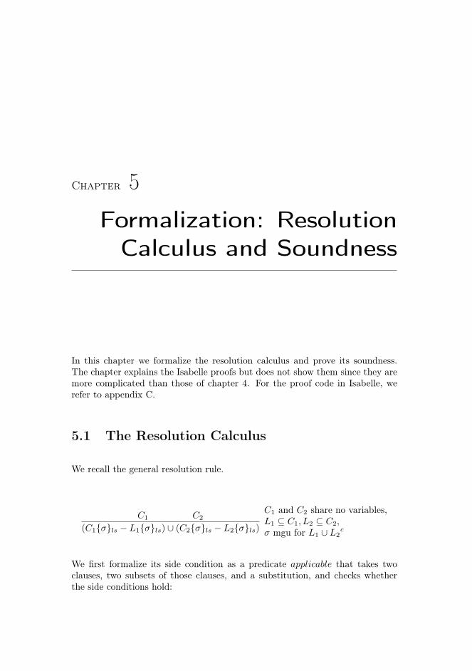
Chapter 5
Formalization: ResolutionCalculus and Soundness
In this chapter we formalize the resolution calculus and prove its soundness.The chapter explains the Isabelle proofs but does not show them since they aremore complicated than those of chapter 4. For the proof code in Isabelle, werefer to appendix C.
5.1 The Resolution Calculus
We recall the general resolution rule.
C1 C2
(C1{σ}ls − L1{σ}ls) ∪ (C2{σ}ls − L2{σ}ls)
C1 and C2 share no variables,L1 ⊆ C1, L2 ⊆ C2,σ mgu for L1 ∪ L2
c
We first formalize its side condition as a predicate applicable that takes twoclauses, two subsets of those clauses, and a substitution, and checks whetherthe side conditions hold:
58 Formalization: Resolution Calculus and Soundness
definition applicable :: fterm clause ⇒ fterm clause⇒ fterm literal set ⇒ fterm literal set⇒ substitution ⇒ bool where
applicable C 1 C 2 L1 L2 σ ←→C 1 6= {} ∧ C 2 6= {} ∧ L1 6= {} ∧ L2 6= {}∧ varsls C 1 ∩ varsls C 2 = {}∧ L1 ⊆ C 1 ∧ L2 ⊆ C 2
∧ mguls σ (L1 ∪ L2C)
Note that we added the extra condition that L1, L2, C1, and C2 should be non-empty, because if C1 or C2 is empty, then we have already derived the emptyclause, and if L1 or L2 is empty, then we will not remove literals from bothclauses.
We formalize the resolution rule as a function that takes C1, C2, L1, L2, and σand gives us the corresponding resolvent.
definition resolution :: fterm clause ⇒ fterm clause⇒ fterm literal set ⇒ fterm literal set⇒ substitution ⇒ fterm clause where
resolution C 1 C 2 L1 L2 σ = (C 1 {σ}ls − L1 {σ}ls) ∪ (C 2 {σ}ls − L2 {σ}ls)
We also define the steps that we use to form derivations. It is defined as a pred-icate resolution-step. Here, resolution-step cs cs’ means that we can perform astep from cs to cs ′:
inductive resolution-step :: fterm clause set ⇒ fterm clause set ⇒ bool whereresolution-rule:C 1 ∈ Cs =⇒ C 2 ∈ Cs =⇒ applicable C 1 C 2 L1 L2 σ =⇒
resolution-step Cs (Cs ∪ {resolution C 1 C 2 L1 L2 σ})| standardize-apart :
C ∈ Cs =⇒ var-renaming σ =⇒ resolution-step Cs (Cs ∪ {C {σ}ls})
It is defined as an inductive definition that consists of two rules. The wordinductive means that the only resolution steps are the ones constructed withthese rules [NK14]. The first rule states that if we can apply resolution to twoclauses then we can add one of their resolvents in a step. The second rule statesthat we may add a renamed clause in a step. We can use this to standardizeclauses apart.
Now that we have defined the individual steps, we can define resolution deriva-tions as the predicate resolution-deriv.
5.2 Soundness of the Resolution Rule 59
definition resolution-deriv :: fterm clause set ⇒ fterm clause set ⇒ bool whereresolution-deriv = star resolution-step
We use the star predicate from the Isabelle distribution, which extends a predi-cate to its reflexive transitive closure, i.e. allows us to apply resolution-step zeroor more times to construct a derivation.
5.2 Soundness of the Resolution Rule
Now that we have defined our resolution calculus, we are ready to prove it sound.We will prove soundness by showing that if the premises of the resolution ruleare satisfied in an interpretation, when so is its conclusion. Then the soundnessof the resolution calculus follows by induction.
To prove the resolution rule sound, we first prove that it is sound to apply amost general unifier to a clause. Next we prove that a very simple version ofresolution is sound. We combine these results to prove that the resolution ruleis sound.
5.2.1 Soundness of Substitution
Instead of proving directly that it is sound to apply a most general unifier, weprove the more general result, that it is sound to apply a substitution. We statethis lemma:
lemma subst-sound :assumes asm: evalc F G Cshows evalc F G (C {σ}ls )
The lemma states that if C is satisfied by the interpretation (F,G), then so isC{σ}ls. Let us think about why this is reasonable. The variables in a clauseC are universally quantified. Therefore, we can substitute them with any term,and the result is still satisfied.
However, the above explanation is not formal enough. The problem is that wemix up the syntactic terms with the semantic elements. That the variables in Care universally quantified means that no matter which elements of the universe
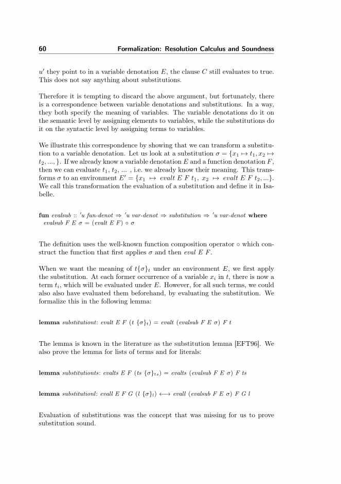
60 Formalization: Resolution Calculus and Soundness
u′ they point to in a variable denotation E, the clause C still evaluates to true.This does not say anything about substitutions.
Therefore it is tempting to discard the above argument, but fortunately, thereis a correspondence between variable denotations and substitutions. In a way,they both specify the meaning of variables. The variable denotations do it onthe semantic level by assigning elements to variables, while the substitutions doit on the syntactic level by assigning terms to variables.
We illustrate this correspondence by showing that we can transform a substitu-tion to a variable denotation. Let us look at a substitution σ = {x1 7→ t1, x2 7→t2, ..., }. If we already know a variable denotation E and a function denotation F ,then we can evaluate t1, t2, ... , i.e. we already know their meaning. This trans-forms σ to an environment E′ = {x1 7→ evalt E F t1, x2 7→ evalt E F t2, ...}.We call this transformation the evaluation of a substitution and define it in Isa-belle.
fun evalsub :: ′u fun-denot ⇒ ′u var-denot ⇒ substitution ⇒ ′u var-denot whereevalsub F E σ = (evalt E F ) ◦ σ
The definition uses the well-known function composition operator ◦ which con-struct the function that first applies σ and then eval E F .
When we want the meaning of t{σ}t under an environment E, we first applythe substitution. At each former occurrence of a variable xi in t, there is now aterm ti, which will be evaluated under E. However, for all such terms, we couldalso also have evaluated them beforehand, by evaluating the substitution. Weformalize this in the following lemma:
lemma substitutiont : evalt E F (t {σ}t) = evalt (evalsub F E σ) F t
The lemma is known in the literature as the substitution lemma [EFT96]. Wealso prove the lemma for lists of terms and for literals:
lemma substitutionts: evalts E F (ts {σ}ts) = evalts (evalsub F E σ) F ts
lemma substitutionl : evall E F G (l {σ}l) ←→ evall (evalsub F E σ) F G l
Evaluation of substitutions was the concept that was missing for us to provesubstitution sound.

5.2 Soundness of the Resolution Rule 61
Proof. We assume that C is satisfied by interpretation (F,G). We haveto prove that C{σ}ls is satisfied by the same interpretation, i.e. that underany variable denotation E, we can find a literal in C{σ}ls that is satisfied.Therefore, we choose an arbitrary variable denotation E and fix it. From ourassumption we know that C is true in (F,G) under any variable denotation.In particular, it is true under the variable denotation evalsub F E σ that weget by evaluating σ. Therefore, there is some literal l, in C that is true under(F,G) and evalsub F E σ. But then, using the substitution lemma, we knowthat l{σ}l must be true under (F,G) and our initial environment E. Thus thereis a literal l{σ}l in C{σ}ls, that is true under (F,G) and E, which means thatC{σ}ls itself is true under (F,G) and E. Since E was chosen arbitrarily, C{σ}lsis true under any interpretation, i.e. C{σ}ls is satisfied by (F,G). Thus, we haveproven instantiation sound. q. e. d.
The Isabelle proof is a straightforward formalization of these arguments.
5.2.2 Soundness of Simple Resolution
We now, as promised, turn to proving the simple resolution rule from chapter 2sound. We recall the rule:
Definition 5.1 (Simple Resolution)
C1 C2
(C1 − {l1}) ∪ (C2 − {l2})
l1 ∈ C1
l2 ∈ C2
l1 = l2c
And state its soundness:
lemma simple-resolution-sound :assumes C 1sat : evalc F G C 1
assumes C 2sat : evalc F G C 2
assumes l1inc1: l1 ∈ C 1
assumes l2inc2: l2 ∈ C 2
assumes Comp: l1c = l2shows evalc F G ((C 1 − {l1}) ∪ (C 2 − {l2}))
The two first assumptions are the assumptions of the soundness property, andthe three next are the side conditions of the rule. In chapter 2 we had anexplanation of the rule, and our soundness proof is similar to this explanation.
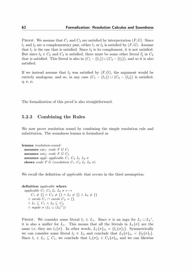
62 Formalization: Resolution Calculus and Soundness
Proof. We assume that C1 and C2 are satisfied by interpretation (F,G). Sincel1 and l2 are a complementary pair, either l1 or l2 is satisfied by (F,G). Assumethat l1 is the one that is satisfied. Since l2 is its complement, it is not satisfied.But since l2 ∈ C2 and C2 is satisfied, there must be some other literal l′2 in C2
that is satisfied. This literal is also in (C1−{l1})∪ (C2−{l2}), and so it is alsosatisfied.
If we instead assume that l2 was satisfied by (F,G), the argument would beentirely analogous, and so, in any case (C1 − {l1}) ∪ (C2 − {l2}) is satisfied.q. e. d.
The formalization of this proof is also straightforward.
5.2.3 Combining the Rules
We now prove resolution sound by combining the simple resolution rule andsubstitution. The soundness lemma is formalized as
lemma resolution-sound :assumes sat1: evalc F G C 1
assumes sat2: evalc F G C 2
assumes appl : applicable C 1 C 2 L1 L2 σshows evalc F G (resolution C 1 C 2 L1 L2 σ)
We recall the definition of applicable that occurs in the third assumption.
definition applicable whereapplicable C 1 C 2 L1 L2 σ ←→
C 1 6= {} ∧ C 2 6= {} ∧ L1 6= {} ∧ L2 6= {}∧ varsls C 1 ∩ varsls C 2 = {}∧ L1 ⊆ C 1 ∧ L2 ⊆ C 2
∧ mguls σ (L1 ∪ (L2C))
Proof. We consider some literal l1 ∈ L1. Since σ is an mgu for L1 ∪ L2c ,
it is also a unifier for L1. This means that all the literals in L1{σ} are thesame i.e. they are l1{σ}. In other words, L1{σ}ls = {l1{σ}l}. Symmetricallywe can consider some literal l2 ∈ L2 and conclude that L2{σ}ls = {l2{σ}l}.Since l1 ∈ L1 ⊆ C1, we conclude that l1{σ}l ∈ C1{σ}ls and we can likewise
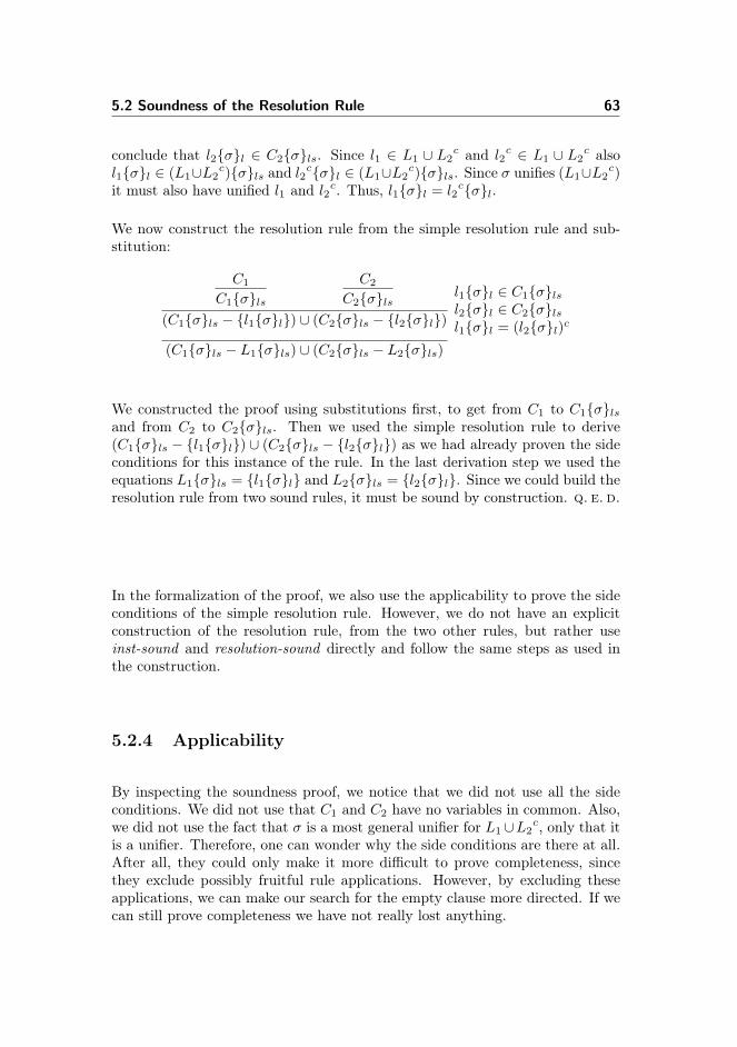
5.2 Soundness of the Resolution Rule 63
conclude that l2{σ}l ∈ C2{σ}ls. Since l1 ∈ L1 ∪ L2c and l2
c ∈ L1 ∪ L2c also
l1{σ}l ∈ (L1∪L2c){σ}ls and l2c{σ}l ∈ (L1∪L2
c){σ}ls. Since σ unifies (L1∪L2c)
it must also have unified l1 and l2c. Thus, l1{σ}l = l2c{σ}l.
We now construct the resolution rule from the simple resolution rule and sub-stitution:
C1
C1{σ}lsC2
C2{σ}ls(C1{σ}ls − {l1{σ}l}) ∪ (C2{σ}ls − {l2{σ}l})
l1{σ}l ∈ C1{σ}lsl2{σ}l ∈ C2{σ}lsl1{σ}l = (l2{σ}l)c
(C1{σ}ls − L1{σ}ls) ∪ (C2{σ}ls − L2{σ}ls)
We constructed the proof using substitutions first, to get from C1 to C1{σ}lsand from C2 to C2{σ}ls. Then we used the simple resolution rule to derive(C1{σ}ls − {l1{σ}l}) ∪ (C2{σ}ls − {l2{σ}l}) as we had already proven the sideconditions for this instance of the rule. In the last derivation step we used theequations L1{σ}ls = {l1{σ}l} and L2{σ}ls = {l2{σ}l}. Since we could build theresolution rule from two sound rules, it must be sound by construction. q. e. d.
In the formalization of the proof, we also use the applicability to prove the sideconditions of the simple resolution rule. However, we do not have an explicitconstruction of the resolution rule, from the two other rules, but rather useinst-sound and resolution-sound directly and follow the same steps as used inthe construction.
5.2.4 Applicability
By inspecting the soundness proof, we notice that we did not use all the sideconditions. We did not use that C1 and C2 have no variables in common. Also,we did not use the fact that σ is a most general unifier for L1∪L2
c, only that itis a unifier. Therefore, one can wonder why the side conditions are there at all.After all, they could only make it more difficult to prove completeness, sincethey exclude possibly fruitful rule applications. However, by excluding theseapplications, we can make our search for the empty clause more directed. If wecan still prove completeness we have not really lost anything.
64 Formalization: Resolution Calculus and Soundness
5.3 Soundness of Resolution Derivations
We now show that a step in a resolution derivation is sound. There are twocases to consider, namely the one where we apply the resolution rule, and theone where we rename variables to standardize clauses apart. We have alreadyproven the resolution rule sound so this case follows easily. When we standardizeapart we apply a substitution, and since we proved substitution sound this casealso follows easily.
lemma sound-step: resolution-step Cs Cs ′ =⇒ evalcs F G Cs =⇒ evalcs F G Cs ′
We can extend the result to a whole derivation. The proof is by induction.Isabelle provides an induction rule called star.induct for the star function thatwe used to define derivations.
lemma sound-derivation:resolution-deriv Cs Cs ′ =⇒ evalcs F G Cs =⇒ evalcs F G Cs ′

Chapter 6
Formalization:Completeness
This chapter formalizes the completeness of the resolution calculus. The chap-ter uses the semantic tree approach from chapter 3. Therefore, it consists of aformal definition of Herbrand terms, enumerations, and semantic trees. Here-after it presents formal proofs of two major steps towards completeness, namelyKönig’s lemma, and Herbrand’s theorem. It also shows the formal statements ofthe lifting lemma and the completeness theorem, and proves the completenesstheorem thoroughly albeit informally.
6.1 Herbrand Terms
We now formalize Herbrand interpretions. These interpretations have two im-portant properties. The first is that their universe consists of herbrand terms.The type of Herbrand terms is similar to that of first-order terms except that itdoes not contain variables:
datatype hterm = HFun fun-sym hterm list

66 Formalization: Completeness
Therefore, Herbrand terms correspond to ground terms. We call atoms Her-brand atoms, if they consist of Herbrand terms, i.e. are literals of type hterm literal .These atoms correspond to ground atoms.
We illustrate the correspondence between ground terms and Herbrand terms byintroducing functions that convert between hterms that are ground, and hterms:
primrec fterm-of-hterm :: hterm ⇒ ftermand fterms-of-hterms :: hterm list ⇒ fterm list wherefterm-of-hterm (HFun p ts) = Fun p (fterms-of-hterms ts)| fterms-of-hterms [] = []| fterms-of-hterms (t#ts) = fterm-of-hterm t # fterms-of-hterms ts
primrec hterm-of-fterm :: fterm ⇒ htermand hterms-of-fterms :: fterm list ⇒ hterm list wherehterm-of-fterm (Fun p ts) = HFun p (hterms-of-fterms ts)| hterms-of-fterms [] = []| hterms-of-fterms (t#ts) = hterm-of-fterm t # hterms-of-fterms ts
The functions are defined using mutual recursion. They only use primitiverecursion which is why we can define them using primrec, but we could alsohave used fun.
The second important property of herbrand interpretations is that their functiondenotation is the constructor HFun. We call it the Herbrand function denota-tion. The constructor HFun has type fun-sym ⇒ hterm list ⇒ hterm whichis the same as hterm fun-denot, and hence its universe is indeed the herbranduniverse. It is a natural function denotation to define, since it simply packs upits input in an hterm. When we evaluate a ground term, we really just apply thefunction denotation recursively to a term, and therefore, evaluating a groundterm under HFun constructs the conversion of the term to an hterm.
We can prove this formally in Isabelle by induction:
lemma eval-ground : ground t =⇒ (evalt E HFun t) = hterm-of-fterm t grounds ts=⇒ (evalts E HFun ts) = hterms-of-fterms ts

6.2 Enumerations 67
6.2 Enumerations
To put labels on the different levels of the semantic tree, we need an enumerationof Herbrand atoms, that is, an infinite sequence A0, A1, A2, . . . of ground atoms,that contains all herbrand atoms.
Two types in Isabelle are very well suited for representing enumerations. Oneis hterm literal stream, and the other is nat⇒ hterm literal.
The hterm stream is a type that represents infinite lists of hterms. Like list, itcomes with a cons operation ##, a head function shd and a tail function stl.The stream library comes with functions that can be used to build up streamsfrom other streams. Therefore, we could first build a stream of strings, then usethat to build a stream of terms, and lastly use that to build a stream of atoms.This is an easy way to build an enumeration from the ground up.
The function type nat ⇒ hterm does not have the nice functions to build upstreams from each other. However, an enumeration of Herbrand terms hasalready been formalized by Berghofer [Ber07]. He does it by defining a nat ⇒hterm function called hterm-diag whose domain consists of all hterms. Therefore,we choose to adapt his enumeration and extend it to enumerations of Herbrandatoms, and ground atoms.
We present our enumeration of herbrand terms:
definition diag-hatom :: nat ⇒ hterm literal wherediag-hatom a ≡
(let (p,ts) = diag a in(Pos (diag-string p) (diag-list diag-hterm ts))
)
We do not go in to details, but notice that it combines three other enumerations:diag, diag-string, and diag-list.
We also present the inverse function, which given an atom, returns the corre-sponding number:
definition undiag-hatom :: hterm literal ⇒ nat whereundiag-hatom a ≡ undiag (undiag-string (get-pred a), undiag-list undiag-hterm
(get-terms a))
68 Formalization: Completeness
Lastly, we present the corresponding functions for ground atoms. We reuse theabove functions by converting the ground atoms to herbrand atoms:
definition diag-fatom :: nat ⇒ fterm literal wherediag-fatom n = fatom-of-hatom (diag-hatom n)
definition undiag-fatom :: fterm literal ⇒ nat whereundiag-fatom t = undiag-hatom (hatom-of-fatom t)
We notice that the enumeration does not consider whether the literal is positiveor negative. This means that we can call undiag-hatom on a negative literal andget the number of the complement atom.
The definitions of all the enumerations and all the lemmas about them areincluded in appendix A.
6.3 Semantic Trees and Partial Interpretations
The core of our completeness proof is to take a semantic tree and to cut it downto the root by looking at the partial interpretations it contains. We thereforealso need to represent partial interpretations. In the literature, semantic treesare usually represented as labeled binary trees. In a well-formed semantic tree,the label of the left children on the i’th level is diag-fatom i, and the label of theright children on the i’th level is complementary (diag-fatom i). A path in thetree can then be converted to a partial interpretation by collecting the labels onthe path in a set of literals that represents the partial predicate denotation. Wepresented these definitions in chapter 3, and they could be implemented directlyin Isabelle.
We choose another approach that illustrates the correspondence between pathsand partial interpretations more clearly. We instead represent the semantic treesas unlabeled binary trees.
datatype tree =Leaf| Branch (ltree: tree) (rtree: tree)
We do not need the labels, since we can always calculate them from the positionof an unlabeled node. This representation has the advantage that we do not

6.3 Semantic Trees and Partial Interpretations 69
need to worry about well-formedness, since the label on the nodes only existimplicitly. This removes junk trees that are not semantic such as the one inwhich all labels are Atom ”p” [].
Paths in a binary tree are modeled as lists of elements of the type dir.
datatype dir = Left | Right
A path corresponds to the process of walking from the root, by iterating overthe list and walking left or right in the binary tree.
For representing partial predicate denotations, we choose the type bool list whereTrue on the i’th position means that diag-fatom i is true in the partial predicatedenotation and False means that diag-fatom i is false. In other words, thepartial predicate denotation assigns truth-values to the ground atoms.
type-synonym partial-pred-denot = bool list
Instead of using defining dir as the above datatype we can define Left and Rightas synonyms of True and False. Then we see that the paths in the binary treeare actually partial predicate denotations.
type-synonym dir = booldefinition Left :: bool where Left = Truedefinition Right :: bool where Right = False
This gives us a simple definition of paths and this definition also representspartial interpretations. The equality of paths and partial interpretations servesas a pedagogical point and gives us the advantage that we do not need lemmasthat describe the correspondence between these concepts.
We choose to represent trees as a datatype. This means that we have definedthe trees as being of finite size. However, semantic trees can also be infinite. InIsabelle we can easily expand the definition to infinite trees by using instead acodatatype:
codatatype tree =Leaf| Branch (ltree: tree) (rtree: tree)

70 Formalization: Completeness
This codatatype represents both finite and infinite trees, in other words, pos-sibly infinite trees. The stream type is another example of a codatatype. Thecodatatypes are a recent addition to Isabelle. Proving properties about co-datatypes is a skill in itself that I assess would take me considerable time tounderstand in depth and learn how to use. Therefore, we chose another ap-proach.
We represent finite trees by the tree datatype, and possibly infinite trees as thetype dir list set. A dir list set represents a tree by consisting of all the pathsthat are in the tree. For a tree to be well-formed, any prefix of a path in thetree must also be a path in the tree. We formalize this property:
abbreviation wf-tree :: dir list set ⇒ bool wherewf-tree T ≡ (∀ ds d . (ds @ d) ∈ T −→ ds ∈ T )
We likewise need a representation for infinite paths in the trees. This is anotherchance to use streams. Instead we choose to use functions of type nat⇒ dir list.The idea is that can represent an infinite path by a function f , where f n givesof the prefix of the path with length n. We call such a function a list chain, anddefine it formally:
abbreviation list-chain :: (nat ⇒ ′a list) ⇒ bool wherelist-chain f ≡ (f 0 = []) ∧ (∀n. ∃ a. f (Suc n) = (f n) @ [a])
We will often consider subtrees rooted in some node of a tree. We define thisconcept:
fun subtree :: dir list set ⇒ dir list ⇒ dir list set wheresubtree T r = {ds ∈ T . ∃ ds ′. ds = r @ ds ′}
The definition takes the path to a node, and then returns the set of paths thatpass through this node, i.e. have it as a prefix.
6.4 König’s Lemma
Our first step in cutting down semantic trees is König’s lemma. The lemmastates that any infinite binary tree contains an infinite path. The contrapositive

6.4 König’s Lemma 71
of this is that a binary tree in which all paths are finite is also finite. Therefore,we can use the theorem to cut trees down to finite size.
We first prove that one of the subtrees T1 and T2 of any infinite tree T is alsoinfinite.
lemma inf-subs:assumes inf : ¬finite(subtree T ds)shows ¬finite(subtree T (ds @ [Left ])) ∨ ¬finite(subtree T (ds @ [Right ]))
Proof. We prove it in its contrapositive formulation: If both the subtrees T1and T2 of a tree T are finite then so is T .
The theorem is now obvious, since T consists of the finite number of notes inT1 plus the finite number of notes in T2 plus the root note of T . This is clearlyfinite. q. e. d.
We now present König’s lemma and its proof in natural language.
Theorem 6.1 Any infinite tree T contains an infinite path.
Proof. We construct the path as follows. Since T is finite, we know from theprevious lemma that either the left subtree T1 or the right subtree T2 is infinite.If T1 is infinite, the first step of the infinite path is Left and then we continuethis process on T1 to get the following steps. If T1 is not infinite, then it wasT2 which was infinite and then we let Right be the first step in the path andthen continue this process on T2 to get the following steps in infinite the path.q. e. d.
The formalization of the lemma is
lemma konig :assumes inf : ¬finite Tassumes wellformed : wf-tree Tshows ∃ c. list-chain c ∧ (∀n. (c n) ∈ T )
72 Formalization: Completeness
The assumptions state that T is an infinite and well-formed tree. The thesisis that there is some list-chain, all of whose prefixes are in T , i.e., there is aninfinite path in T .
To formalize this proof we need a way to pick the infinite subtrees. For thispurpose, we define the function ?nextnode. We can call it on an node that isthe root of an infinite subtree, and then it returns the path to the left subtreeif it is infinite and otherwise the path to the right subtree, which must then beinfinite.
let ?nextnode =λds. (if ¬finite(subtree T (ds @ [Left ])) then ds @ [Left ] else ds @ [Right ])
The function is defined inside the proof as a schematic variable. This is some-what similar to the abbreviations, since it just defines ?nextnode as a syntacticalshorthand for its definition.
We also define the function buildchain. Given a natural number n and a functionnext of type dir list⇒ dir list it starts from [] and then applies next to it n times.
fun buildchain :: (dir list ⇒ dir list) ⇒ nat ⇒ dir list wherebuildchain next 0 = []| buildchain next (Suc n) = next (buildchain next n)
This is enough for us to construct our list-chain:
let ?c = buildchain ?nextnode
Of course, we need to show that it is actually a list-chain. This can be shownwith auto. It is also easy to realize, since ?nextnode always appends an elementto the end of the previous list.
We also need to show that for any n, the path ?c n is in T . We prove ageneralization of this by induction on the natural number n. The generalizationis that ?c n is in the tree, and that the subtree rooted in ?c n is infinite.We need to make this generalization because ?nextnode only gives us a newinfinite subtree, if we call it on the root of an infinite subtree. Therefore, in ourinduction, we need to carry this information in our induction hypothesis.
It is easy to prove for the base case of 0. Since T is infinite, it must containsome path ds, and since the tree is well-formed, it must also contain the prefix

6.5 Semantics of Partial Predicate Denotations 73
[], but [] is actually ?c 0. The subtree rooted in ?c 0 = [] is actually the wholetree, and it is infinite by assumption.
We also prove the induction case, i.e. prove the theorem for n+1. The inductionhypothesis is that that ?c n is in T , and that the subtree rooted in ?c n is infinite.We must prove the same property for n + 1. By the induction hypothesis, thesubtree rooted in ?c n is infinite. Therefore we can apply ?nextnode to get anew infinite subtree ?nextnode (?c n). We recall that by definition of ?c, andof buildchain, we know that ?c n consists of n applications of ?nextnode. Thus,?nextnode (?c n) must be n+1 applications of ?nextnode, i.e., ?c (n+1). So thesubtree roted in ?c (n+ 1) is infinite. This also means that there must be somepath ds in the subtree, and ?c (n+1) must surely be a prefix of this. Therefore,since the T well-formed, ?c (n+ 1) must also be in T .
This concludes our formalization of König’s lemma.
6.5 Semantics of Partial Predicate Denotations
Let us introduce the semantics for partial predicate denotations. We first in-troduce their semantics for literals. Our semantics is optimistic with regard tosatisfying literals. If the partial predicate denotation does not contain enoughinformation about a literal to actively falsify it, then it does not falsify it, butsatisfies it.
A partial predicate denotation assigns truth-values to ground atoms. It falsifiesan atom if it assigns False to an instance of the atom. Likewise, it falsifies anegative literal if it assigns True to an instance of the complementary atom.
fun falsifiesl :: partial-pred-denot ⇒ fterm literal ⇒ bool wherefalsifiesl G (Pos p ts) =
(∃ i ts ′.i < length G∧ G ! i = False∧ diag-fatom i = Pos p ts ′
∧ instance-ofts ts ′ ts)| falsifiesl G (Neg p ts) =
(∃ i ts ′.i < length G∧ G ! i = True∧ diag-fatom i = Pos p ts ′
∧ instance-ofts ts ′ ts)

74 Formalization: Completeness
For a positive literal Pos p ts, it is done by looking if there is an entry in Gcontaining an atom that is an instance of the literal, and is assigned to False.The definition for negative literals mirrors this.
A partial predicate denotation G is said to satisfy a literal if it does not falsifyit. In other words, an atom is satisfied if all instances of it in G are assignedto True. Likewise, a negative literal is satisfied if all instances of it in G areassigned to False.
A partial predicate denotation falsifies a clause by falsifying some literal in theclause, and it falsifies a clausal form by falsifying some clause in the clausalform:
abbreviation falsifiesc :: partial-pred-denot ⇒ fterm clause ⇒ bool wherefalsifiesc G C ≡ (∀ l ∈ C . falsifiesl G l)
abbreviation falsifiescs :: partial-pred-denot ⇒ fterm clause set ⇒ bool wherefalsifiescs G Cs ≡ (∃C ∈ Cs. falsifiesc G C )
We can use this to formalize closed and open branches. To do that, we mustfirstly formalize branches.
inductive branch :: dir list ⇒ tree ⇒ bool wherebranch [] Leaf| branch ds l =⇒ branch (Left # ds) (Branch l r)| branch ds r =⇒ branch (Right # ds) (Branch l r)
The definition says that the empty list is a subtree of a leaf, and that if thetail of a list is a branch of an immediate left subtree, then if we add Left tothe beginning we have a branch of the whole tree, and similarly for the rightsubtree. Since it is inductive, it also states that these are the only branches.
We have again used an inductive predicate. A closed branch for a clausal formis a branch that falsifies the clausal form. An open branch is a branch that doesnot.
abbreviation closed-branch :: partial-pred-denot ⇒ tree ⇒ fterm clause set ⇒ boolwhereclosed-branch G T Cs ≡ branch G T ∧ falsifiescs G Cs
6.6 Herbrand’s Theorem 75
abbreviation open-branch :: partial-pred-denot ⇒ tree ⇒ fterm clause set ⇒ boolwhereopen-branch G T Cs ≡ branch G T ∧ ¬falsifiescs G Cs
A closed tree is a finite tree in which the branches and only the branches areclosed:
fun closed-tree :: tree ⇒ fterm clause set ⇒ bool whereclosed-tree T Cs ←→ anybranch T (λb. closed-branch b T Cs)
∧ anyinternal T (λp. ¬falsifiescs p Cs)
6.6 Herbrand’s Theorem
Herbrand’s theorem comes in several versions [CL73]. We prove the followingversion:
Theorem 6.2 If a clausal form Cs is unsatisfiable then there exists a finite andclosed semantic tree for Cs.
We first prove the theorem in the following slightly different and contrapositiveformulation:
Lemma 6.3 If all finite semantic trees of a clausal form Cs have an openbranch, then Cs has a model.
6.6.1 Building a Model
We will use König’s lemma to find an infinite path G, all of whose prefixesare partial predicate denotations that satisfy Cs. The infinite path G can beseen as an infinite partial predicate denotation. This is the same as a predicatedenotation because it assigns a truth value to any predicate symbol and list ofelements of the Herbrand universe.
Before we find it, we show that it also satisfies Cs. It might seem obvious,but it does require substantial work that illustrates the interplay of syntax andsemantics similarly to our soundness proof.
76 Formalization: Completeness
Lemma 6.4 If G is an infinite path and all its prefixes satisfy a clausal formCs, then G itself also satisfies Cs.
Proof. We fix an arbitrary variable denotation E and a clause C in Cs, toshow that any clause in Cs is true under any variable denotation.
Since our universe is Herbrand terms, the variable denotation E has type var-sym⇒hterm. Therefore, we can easily create a function sub-of-denot that turns it intoa substitution σ, by converting its domain from hterms to ground terms. Thismirrors our soundness proof, where we converted substitution to variable deno-tations.
fun sub-of-denot :: hterm var-denot ⇒ substitution wheresub-of-denot E = fterm-of-hterm ◦ E
Using the substitution σ on our clause, we get a new clause C{σ}ls with thefollowing properties:
a. C{σ}ls is ground. This is because the domain of σ consists of ground terms.
b. Under E and HFun, both C and C{σ}ls are satisfied and falsified by thesame predicate denotations. The reason is this: We consider a variable xthat occurs in C. The variable will be evaluated to an Herbrand term h. Ifwe look at C{σ}ls, the variable is first replaced by h’s conversion to a term.Then this term is evaluated by HFun and thus converts to h again. So inboth cases x evaluates to h.
c. If C{σ}ls is falsified by a partial predicate denotation G′, then so is C. Thata literal l{σ}l in C{σ}ls is falsified by G′, means that G′ falsifies some groundinstance of l{σ}l. This ground instance is also an instance of l, and so, alsol in C is also falsified.
d. If C is satisfied by a partial predicate denotation, then so is C{σ}ls. This isthe contrapositive of item c.
Thus, by item b, to prove that C is satisfied by G, it suffices to show thatG satisfies C{σ}ls. Take a prefix G′ of the full predicate denotation G, suchthat G′ is large enough that it covers all literals in C{σ}ls. It satisfies C (byour assumption) and thus also C{σ}ls (by item d). So must G since it is anextension of G′, and extending it only adds assignments of True and False toirrelevant literals that are not in C{σ}ls. q. e. d.
6.6 Herbrand’s Theorem 77
In the above proof, we looked at an infinite path G that we had gotten fromKönig’s lemma, and argued that it was a predicate denotation. But we rememberthat our formalization of König’s lemma actually gives us a list-chain of paths.
Therefore, we make a function that converts a list-chain to a predicate denota-tion.
abbreviation extend :: (nat ⇒ partial-pred-denot) ⇒ hterm pred-denot whereextend f P ts ≡ (
let n = undiag-hatom (Pos P ts) inf (Suc n) ! n
)
We call the function extend, because extend f can be seen as an extension of anyf n. When we give a predicate symbol p and an hterm list ts to extend f , thenit finds the number n of the atom Pos p ts, and then it finds a prefix f (Suc n)in that is long enough to contain n. Then it looks up whether the n′th entryassigns Pos p ts to True or False.
With this cleared up we present our formalization of this lemma:
lemma extend-preserves-model :assumes f-chain: list-chain (f :: nat ⇒ partial-pred-denot)assumes n-max : ∀ l∈C . undiag-fatom l ≤ nassumes C-ground : groundls Cassumes C-false: ¬evalc HFun (extend f ) Cshows falsifiesc (f (Suc n)) C
6.6.2 Proving Herbrand’s Theorem
We are now ready to prove Herbrand’s theorem by finding our infinite path.
Proof. We build a semantic tree T from a clausal form Cs. It consists of allpaths that, when seen as a partial predicate denotations, satisfiy Cs.
We now show that this tree is infinite by generating infinitely many differentpaths that are contained in this tree: We consider some other semantic tree thatis finite. From our assumption we know that this tree has an open branch. Thisis true no matter what the depth of that tree is. So we can build a semantictree of depth 1, to get an open branch of length 1. Since it is open, it does notfalsify any ground instance of any clause. Therefore this path is also a path in

78 Formalization: Completeness
T . We can do the same for a semantic tree of depth 2, and one of depth 3, andso on. Thus the tree is infinite.
Now we can use König’s lemma to obtain an infinite path G in T . All itsprefixes are satisfying partial predicate denotation, and we already showed thatthis implies that G also satisfies C. q. e. d.
We formalize the lemma and its proof in Isabelle.
theorem herbrand ′:assumes openb: ∀T . ∃G. open-branch G T Csassumes finite-cs: finite Cs ∀C∈Cs. finite Cshows ∃G. evalcs HFun G Cs
This was our second formulation of Herbrand’s lemma. We would also like toprove the first one. We first take the contra-positive of herbrand′:
theorem herbrand ′-contra:assumes finite-cs: finite Cs ∀C∈Cs. finite Cassumes unsat : ∀G. ¬evalcs HFun G Csshows ∃T . ∀G. branch G T −→ closed-branch G T Cs
We see that we have a tree in which all the branches are closed. However, wewanted exactly the branches to be closed. We can obtain such a tree by cuttingbranches off as soon as they are long enough to falsify a clause.
This cutting of branches is formalized by introducing tree operations that canremove nodes, and proving a quite substantial amount of theorems about them.They are not presented here because they do not give much logical insight.Instead we present the formalization of Herbrand’s lemma and refer to appen-dices B and C.
theorem herbrand :assumes unsat : ∀G. ¬ evalcs HFun G Csassumes finite-cs: finite Cs ∀C∈Cs. finite Cshows ∃T . closed-tree T Cs
The proof simply combines herbrand’-contra with the tree operations.
6.7 Lifting Lemma 79
6.7 Lifting Lemma
Our next step is to prove the lifting lemma. We first state it:
lemma lifting :assumes appart : varsc c ∩ varsc d = {}assumes inst1: instance-ofc c ′ cassumes inst2: instance-ofc d ′ dassumes appl : applicable c ′ d ′ l ′ m ′ σshows ∃ l m τ . applicable c d l m τ ∧
instance-ofc (resolution c ′ d ′ l ′ m ′ σ) (resolution c d l m τ)
This thesis does not contain a formalized proof of this lemma, because it turnedout to be much more challenging than expected. The main reason was thatseveral proofs of the lemma from the literature were flawed. In chapter 8, wewill discuss this challenge, as well as possibilities for overcoming it. For now,we turn to the completeness proof.
6.8 Completeness
Assuming a proof of the lifting lemma, we have all the theory necessary to provethe resolution calculus complete. We state the completeness theorem:
theorem completeness:assumes finite-cs: finite Cs ∀C∈Cs. finite Cassumes unsat : ∀F G. ¬evalcs F G Csshows ∃Cs ′. resolution-deriv Cs Cs ′ ∧ {} ∈ Cs ′
I used quite a lot of time trying to make a formalized proof of the lifting lemma.Therefore, I did not have time to also formalize a proof of the completenessitself. Furthermore, the correctness of such a proof would depend entirely on thecorrectness of the lifting lemma. We will therefore instead look at an informal,but thorough, proof of the theorem, which can form the basis of its formalization.The proof follows the one from chapter 3, but uses the definitions of the Isabelleformalization.
Proof. Since our clausal form Cs is unsatisfiable, it must by Herbrand’s lemmahave a finite closed semantic tree. Our proof is by induction on the size of this

80 Formalization: Completeness
tree T and for arbitrary clausal forms. We therefore restate the completenesslemma to assume the existence of the finite closed semantic tree, such that itwill be part of our induction hypothesis.
theorem completeness ′:assumes finite-cs: finite Cs ∀C∈Cs. finite Cshows closed-tree T Cs =⇒ ∃Cs ′. resolution-deriv Cs Cs ′ ∧ {} ∈ Cs ′
If the tree has size 1, then it must consist only of a leaf node. The empty list [] isa branch in this tree. By definition of closed semantic trees, we know that theremust be some clause C ∈ Cs that [] falsifies, i.e. it has to falsify all of the literalsin C. The only clause that [] can falsify is {} because any other clause containsa literal that [] does not falsify. Thus {} ∈ Cs and we have hence derived theempty clause.
We also prove it for the induction case of trees of size n > 1. Our inductionhypothesis is that we can derive the empty clause from any clausal form Cs′
with a closed semantic tree T ′ of size smaller than T .
We must prove that we can also derive the empty clause from Cs using oursemantic tree T . We find a node N in T , whose children N1 and N2 are leafs.The existence of this node can be proven by induction on trees. Now, we considerthe path B from the root to N , the branch B1 from the root to N1, and thebranch B2 from the root to N2. By the definition of semantic trees, we knowthat B1 = B @ [True] and B2 = B @ [False]. Furthermore, we know thatthere exists some clause C1 that has a ground instance C ′1 that is falsified byB1. Likewise there is a C2 and a C ′2 corresponding to B2. Since C ′1 is falsifiedby B @ [True], all the literals in C ′1 must be falsified by this list. But theyare not all falsified by B, since it is not a branch node. Therefore there mustbe a literal l1 ∈ C1 that is falsified by B @ [True], but not by B. This literalmust have number |B| + 1 in our enumeration, since it is the only one that isfalsified by B @ [True] but not B. It must also be negative. Additionally, allthe other literals in C ′1 must be falsified by B, since they are falsified by B1, butnot l′1. Likewise C ′2 must contain l′2 which is the positive literal with number|B|+1. Therefore C ′1 and C ′2 have a clashing pair of literals, and we can performresolution to get a resolvent C ′. The resolvent C ′ must be falsified by B sinceresolving C ′1 and C ′2 removes the only two of their literals that were not falsifiedby B. By the lifting lemma, we can obtain the resolvent C of C1 and C2 withinstance C ′. We create a new tree T ′ which is T with N1 and N2 removed, anda new clause set Cs′ = Cs∪{C}. Since C ′ is falsified by the branch B of T ′, andall other branches of B′ are already closed, we can cut T ′ down to a closed treefor Cs ∪ {C} using the tree operations for that we used in Herbrand’s theoremto cut branches.

6.8 Completeness 81
By the induction hypothesis we can derive the empty clause from Cs′. Thisgives us the following derivation of the empty clause from Cs: From Cs wederive Cs′ = Cs ∪ {C} using the resolution rule. Then from that, we derive theempty clause. q. e. d.

82 Formalization: Completeness
Chapter 7
Examples
In this section we show some formalizations of resolution derivations in ourresolution calculus. We start with the derivation we presented in chapter 2.This derivation works on ground clauses. Therefore, the complementary sets ofliterals each contain one element. This means that any substitution is a unifier,including the empty substitution. Furthermore, the empty substitution is anmgu, since we can construct any substitution from it.
theorem unifier-single: unifierls σ {l}
theorem empty-mgu: unifierls ε L =⇒ mguls ε L
We define the literals of the clauses.
definition PP :: fterm literal wherePP = Pos ′′P ′′ [Fun ′′c ′′ []]
definition PQ :: fterm literal wherePQ = Pos ′′Q ′′ [Fun ′′d ′′ []]
definition NP :: fterm literal where
84 Examples
NP = Neg ′′P ′′ [Fun ′′c ′′ []]
definition NQ :: fterm literal whereNQ = Neg ′′Q ′′ [Fun ′′d ′′ []]
The first letter, P or N indicates if the literal is positive or negative, and thenext letter P or Q, indicates if the predicate symbol is P or Q. We present theformalization of our derivation:
lemma resolution-example1 :∃Cs. resolution-deriv {{NP ,PQ},{NQ},{PP ,PQ}}
{{NP ,PQ},{NQ},{PP ,PQ},{NP},{PP},{}}
We see that the empty clause can indeed be derived. I have not included theproof, but it essentially consists of spelling out each derivation step as a proofstatement in Isabelle. It is included in appendix D. The full derivation is thenproven using the simplification rules of resolution-deriv.
We can also prove the example we looked at in chapter 3 as an example of howthe completeness proof works. Again we define the literals first:
definition Pa :: fterm literal wherePa = Pos ′′a ′′ []
definition Na :: fterm literal whereNa = Neg ′′a ′′ []
definition Pb :: fterm literal wherePb = Pos ′′b ′′ []
definition Nb :: fterm literal whereNb = Neg ′′b ′′ []
definition Paa :: fterm literal wherePaa = Pos ′′a ′′ [Fun ′′a ′′ []]
definition Naa :: fterm literal whereNaa = Neg ′′a ′′ [Fun ′′a ′′ []]
definition Pax :: fterm literal wherePax = Pos ′′a ′′ [Var ′′x ′′]
definition Nax :: fterm literal whereNax = Neg ′′a ′′ [Var ′′x ′′]

85
We also need a most general unifier for the terms a(a()) and a(x):
definition mguPaaPax :: substitution wheremguPaaPax = (λx . if x = ′′x ′′ then Fun ′′a ′′ [] else Var x )
lemma mguPaaPax-mgu: mguls mguPaaPax {Paa,Pax}
It takes considerable work to prove that it is an mgu. For the formalized proof,we refer to appendix C. With a formalization of a unification algorithm, wecould just calculate an mgu instead of explicitly proving its existence.
We can now perform the derivation:
lemma resolution-example2 :∃Cs. resolution-deriv {{Nb,Na},{Pax},{Pa},{Na,Pb,Naa}}
{{Nb,Na},{Pax},{Pa},{Na,Pb,Naa},{Na,Pb},{Na},{}}
Finally, using our soundness lemma, we show that since we can derive the emptyclause in the examples, the clausal forms are indeed unsatisfiable. We first provethat if we can derive the empty clause from a clausal form, then it is satisfiable:
lemma ref-sound :assumes deriv : resolution-deriv Cs Cs ′ ∧ {} ∈ Cs ′
shows ¬evalcs F G Cs
We then apply this theorem to our examples:
lemma resolution-example1-sem: ¬evalcs F G {{NP , PQ}, {NQ}, {PP , PQ}}
lemma resolution-example2-sem: ¬evalcs F G {{Nb,Na},{Pax},{Pa},{Na,Pb,Naa}}

86 Examples
Chapter 8
Discussion
This chapter discusses the formalization of the resolution calculus.
• It discusses proofs of the lifting lemma from the literature.
• It suggests solutions obtaining a formalized proof of the lifting lemma.
• It discusses the relation the formalization of the resolution calculus toautomated theorem provers.
• It discusses the lessons I have learned during the formalization process.
• It discusses the thesis itself.
8.1 Proving the Lifting Lemma
The formalization does not yet have a formal proof of completeness. To obtain aproof, there are two hurdles to overcome. First, we must prove the lifting lemma,and then we must use it to prove completeness. In chapter 6, we already hada thorough proof of completeness that could be formalized, and therefore, thelarger challenge is formalizing a proof of the lifting lemma.

88 Discussion
Formalizing a proof of the lifting lemma turned out to be more of a challengethan I expected. The reason is that the presentations I studied turned out notto be well suited for a formalization, because they had some flaws that couldnot easily be resolved. In this section, we will study a proof from the literature.We observe some flaws and discuss how to resolve them.
8.1.1 A Proof From the Literature
We will study a proof of the lifting lemma from Ben-Ari’s book MathematicalLogic for Computer Science [BA12]. We will see why the proof can not easilybe formalized, and describe some flaws and imprecisions. The notation anddefinitions are similar to ours, except that substitutions are sets of key-valuepairs writen k ← v, where k is a key and v a value. Thus they can be combinedwith the ∪ operator. A substitution is well-formed if it is finite and maps eachkey to exactly one value. The notation for applying substitutions is lσ and thatfor composition is σ1σ2
Theorem 10.33 (Lifting Lemma) Let C ′1, C ′2 be ground instances of C1,C2, respectively. Let C ′ be a ground resolvent of C ′1 and C ′2. Then there isa resolvent C of C1 and C2 such that C ′ is a ground instance of C.
Proof First, standardize apart so that the names of the variables in C1 aredifferent from those in C2. Let l ∈ C ′1, lc ∈ C ′ be the clashing literals in theground resolution.
Since C ′1 is an instance of C1 and l ∈ C ′1, there must be a set of literalsL1 ⊆ C1 such that l is an instance of each literal in L1. Similarly theremust be a set of literals L2 ⊆ C2 such that lc is an instance of each literalin L2.
The last paragraph is problematic, since with this formulation we can just letL1 = {} and then it contains nothing that can be resolved. I suggest that weinstead obtain a substitution θ such that C1θ = C ′1 and C2θ = C ′2. Then we letL1 be the set of all literals l1 ∈ C1 where l1θ = l, and let L2 be the set of allliterals l2 ∈ C2 where l2θ = l. In this way we catch exactly the clashing sets ofliterals that are to be removed.
Let λ1 and λ2 [be] mgu’s for L1 and L2, respectively, and let λ = λ1∪λ2. λis a well-formed substitution since L1 and L2 have no variables in common.
8.1 Proving the Lifting Lemma 89
This argument strictly does not hold. Here is a counter-example: Let L1 = {c}and L2 = {c}. L1 and L2 have no variables in common. An mgu for L1 isu1 = {x ← y, y ← x}. An mgu for L2 is u2 = {x ← z, z ← x}. Then considerthe union u1 ∪ u2 = {x ← y, y ← x, x ← z, z ← x}. It is not well formed sincex is mapped to both y and z.
I think we can remedy this by requiring that we require λ1 to not substituteany variable that is not in L1, and likewise for L2. In fact, the mgu’s producedby unification algorithms have this property. This flaw is minor, but for aformalization even such small flaws are not allowed.
By construction, L1λ and L2λ are sets which contain a single literal each.These literals have clashing ground instances, so they have a[n] mgu σ.
The argument is presumably that if they have clashing ground instances, thenthey have a unifier and then they have an mgu. Here is another minor flaw:The two literals f(x) and f(f(x)) both have ground instance f(f(c)), but theycannot be unified. This can also be remedied by adding the above restrictionson λ1 and λ2.
Furthermore, this argument is left to the reader: The reason they have clashingground instances. Here is the argument: θ unifies L1 to a ground instance L1θ,so since λ1 is mgu: θ = λ1u1 for some u1. Thus L1θ = L1(λ1u1) = (L1λ1)u1 =(L1λ)u1. Likewise for L2λ.
Since Li ⊆ Ci, we have Liλ ⊆ Ciλ. Therefore, C1λ and C2λ are clausesthat can be made to clash under the mgu σ. It follows that they can beresolved to obtain clause C:
C = ((C1λ)σ − (L1λ)σ) ∪ ((C2λ)σ − (L2λ)σ).
By the associativity of substitution (Theorem 10.10):
C = (C1(λσ)− L1(λσ)) ∪ (C2(λσ)− (L2(λσ)).
C is a resolvent of C1 and C2 provided that λσ is an mgu of L1 and Lc2.
But λ is already reduced to equations of the form x← t for distinct variablesx and σ is constructed to be an mgu, so λσ is a reduced set of equations,all of which are necessary to unify L1 and Lc
2. Hence λσ is an mgu.

90 Discussion
The last two sentences can be difficult to understand. For instance, it is notentirely clear what the author means by a reduced set of equations or how weknow that they are necessary to unify L1 and Lc
2. A more thorough treatmentis necessary for a formalization.
Since C ′1 and C ′2 are ground instances of C1 and C2:
C ′1 = C1θ1 = C1λσθ′1 C ′2 = C2θ2 = C2λσθ
′2
for some substitutions θ1,θ2,θ′1,θ′2. Let θ′ = θ′1 ∪ θ′2.
Substitutions θ1 and θ2 are introduced, corresponding to the θ that I suggestedwe introduced earlier.
We should also argue that θ′ is well formed. To do this we need to make someof the same considerations as for when we made λ. We also have to think abouthow λ and σ were defined.
Then C ′ = Cθ′ and C ′ is a ground instance of C.
Here it is in my opinion not clear why C ′ = Cθ′. I have (unsuccessfully) triedto come up with a proof for it. My attempt follows here:
We want to have that C ′1 = C1λσθ′1 = C1λσθ
′. This should follow from thevariable distinctness of θ′1 and θ′2 as well as from the variable distinctness ofC1λσ and C2λσ. Likewise we argue that C ′2 = C2λσθ
′2 = C2λσθ
′.
Then:C ′ = (C ′1 − {l}) ∪ (C ′2 − {lc})
= (C1λσθ′ − L1λσθ
′) ∪ (C2λσθ′ − L2λσθ
′)
= (C1λσ − L1λσ)θ′ ∪ (C2λσθ
′ − L2λσ)θ′
= ((C1λσ − L1λσ) ∪ (C2λσθ′ − L2λσ))θ
′
= Cθ′
To prove this I used that (A∪B)σ = Aσ ∪Bσ, which holds in general, but also(A − B)σ = Aσ − Bσ which does not hold in general. For instance ({Z,X} −{X}){Z ← X} = {X}, but {Z,X}{Z ← X} − {X}{Z ← X} = {}. Thus myproof attempt is unsuccessful.
8.1 Proving the Lifting Lemma 91
To sum up, the proof has several flaws and imprecisions. They can be summa-rized in five bullet points:
• L1 and L2 are not properly defined.
• It is not enough that C1 and C2 are standardized apart. We also needto make sure that many of the substitutions of the proof preserve thisproperty.
• Union of substitutions is not necessarily well formed under the given con-ditions.
• From the text it is not clear why λσ is an mgu of L1 and Lc2.
• It is not clear why C ′ = Cθ′.
I have pointed to solutions to these flaws and imprecisions except for the lastone, which I am not sure how to address. In appendix E, I repeat the exercise foranother proof, and present a counter-example by Leitsch [Lei89] to that proof.
If we want to prove the lifting lemma, then we must either fix the flaws in theproof somehow, or we must come up with a new proof entirely.
8.1.2 Another Resolution Calculus
Another approach is to use a resolution calculus that has a simpler proof of thelifting lemma. One such resolution calculus is presented by Leitsch [Lei97]. Welook at its definition using the notation of this thesis. It is an example of binaryresolution with factoring, but the binary resolution rule is a little different fromthe one we presented.
Definition 8.1 (Leitsch’s Binary Resolution Rule)
C1 C2
((C1 − {l1}) ∪ (C2 − {l2})){σ}
C1 and C2 have no variables in common,l1 ∈ C1, l2 ∈ C2,σ is an mgu for {l1, lc2}
The difference from our binary resolution rule is that the literals are removedbefore the mgu is applied, instead of the other way round. Letisch presentsa simple proof of the lifting lemma for this resolution calculus. One of itsadvantages is that it does not have the problems of the above proof becauseit avoids the wrong equation (A − B){σ} = A{σ} − B{σ} completely. Otherauthors use similar resolution calculi, including Robinson, who invented theresolution calculus.
92 Discussion
8.1.3 The Unification Algorithm
Another challenge in formalizing the lifting lemma is that its proof assumes theexistence of most general unifiers. That is, if we have a unifier for a set, thenwe also have a most general unifier for the set. The standard way to prove thistheorem is by constructing a unification algorithm and proving it correct. Aunification algorithm is an algorithm that explicitly constructs the most generalunifier.
A shortcut to obtain this goal would be to adapt the unification algorithm ofanother formalization such as that of IsaFoR [TS09].
8.1.4 Recommended Approach
We have identified two approaches to proving the lifting lemma. One is torepair the proof for our current definition, or making a new proof. The otheris to choose a definition of resolution that removes literals before applying themgu.
To achieve the goal of obtaining a formalized complete resolution calculus, I rec-ommend the second approach. It has the clear advantage of having a thoroughpaper proof to follow. The disadvantage is that we need to prove soundnessagain for the new system. However, soundness proofs are simpler than com-pleteness proofs, and our current proof can hopefully be adapted without toomuch effort.
Formalizing the lifting lemma for our current definition of resolution could alsobe an interesting result, because it would confirm that such systems are completeand it would give us a way to repair the proof from Ben-Ari’s textbook.
8.2 Formalizing a Logical System in a LogicalSystem
I have proven the resolution system sound in the logical system of Isabelle’sHOL. Therefore, one can argue that the soundness of my resolution calculusdepends on the soundness on Isabelle. Thus, one could argue, I should alsoprove Isabelle sound. To do this I would need a stronger proof system thanIsabelle since Gödel’s incompleteness theorem tells us that a sound proof system
8.3 Automatic Theorem Proving 93
cannot prove itself sound. But then we must again consider the soundness ofthat stronger logical system. Therefore, one can argue, that we have not reallylearned much by doing this exercise.
However, in our introduction we looked at a proof system such as Isabelle as acollection of arguments that we agree on are true, and from which we constructour proof. In this view, our formalization is at least as good as an informal proof.An informal proof will prove the soundness using a number of mathematicalarguments. Our proof does the same, except that we restrict ourselves to asubset that we agree on beforehand. This also means that we cannot appealto the sometimes faulty human intuition, and that a computer can check if theproof indeed only uses the argument we agreed on. Giving a theorem a proofthat a human can read and understand, and a proof that a computer can checkincreases our confidence in the theorem.
Furthermore, there is good empirical evidence that Isabelle is sound. It is usedby many researchers to formalize many different disciplines of mathematics,computer science, logic, and more. If an unsoundness does occur it can poten-tially be fixed without affecting the theorems proven thus far. Finally, the logicof proof assistants can also be verified formally [Har06].
8.3 Automatic Theorem Proving
As mentioned in the introduction, the resolution calculus has been implementedsuccessfully in automatic theorem provers. It is worth discussing what the im-plications of this formalization of the resolution calculus has on these provers.
Firstly, the formalization increases confidence in the background theory of theseprovers. It also provides through proofs of soundness and completeness, whichcan give a better understanding of these theorems. However, the best of theautomatic theorem provers have additional rules in addition to resolution, suchas superposition rules. These rules are not part of this formalization.
Furthermore, the systems are concrete implementations in a programming lan-guage of a more abstract proof system. This means that even if the full abstractsystem is proven sound and complete, this does not necessarily mean that theconcrete implementation is sound and complete. One way to overcome thisobstacle is to create a verified prover.
Isabelle can generate code in the Standard ML programming language from aformalization. To do this, however, the formalization needs to be specified in a
94 Discussion
way that makes it executable. Our formalization is not at that stage, since we,for instance, have not formalized a unification algorithm. The approach has,however, been used to create a verified prover for another prover [Rid04].
8.4 Societal Perspective
As we have seen, this thesis can be seen as a first step towards a verified au-tomatic prover based on resolution. Provers are highly advanced software andtheir formalization will show that verified software is an obtainable goal. Soft-ware plays a very important role in our society, as increasingly many tools anddevices contain some kind of software. Today the correctness of software ismostly tested by providing it with input and seeing if it behaves as expected.However, it is almost always impossible to test all possible inputs, which meansthat there might be some case in which the program does not behave as ex-pected. A good example is the sorting algorithm of the Java library which wasthoroughly tested, but still contained a bug [dGRdB+15].
Verifying the software formally means that we logically prove the absence ofbugs. Such proofs cover all possible cases, because they explain why the softwareworks on an arbitrary input. This is especially important as software becomesa larger and larger part of our lives. A good example is the verified airplanealerting algorithm [CM00] that we considered in chapter 1, because softwarebugs can have serious consequences in the case of air transport. Thus, theverification of software is important in itself. However, if proof systems are toplay an important role in software verification, it is also important that we gainhigh confidence in their soundness. This thesis is a step in that direction.
8.5 Lessons Learned
I have learned a lot during the process of formalizing resolution. Firstly, Ihave learned that it is important to prepare well. During the first phase of theprocess I studied the literature quite thoroughly and was an advantage whenI had to formalize lemmas and theorem, because I understood them well andgot to know them without thinking about formalization details. This meantthat when I formalized the proofs of König’s lemma and Herbrand’s theorem, Ihad already overcome the challenge of understanding the proofs, and thus couldfocus on formalization.

8.6 Reflections on the Thesis 95
Another lesson that I have learned is that the formalization process can uncoverflaws in proofs. When I initially read the proof of the lifting lemma, I thoughtI understood it. However, the formalization process made me discover its flaws.This mirrors the experience of others.
Additionally, I have learned that the formalization process can lead to moreprecise proofs, and help us understand theorems better. A good example ofthis is my soundness proof. Many of the proofs I read in the literature onlyglanced over this property. The formalization, however, makes the correspon-dence between syntax and semantics very clear by introducing the evaluation ofsubstitutions and proving the substitution lemma formally. The separation ofsyntax and semantics is central to logics, and the formalization makes this veryexplicit.
8.6 Reflections on the Thesis
During the process of writing this thesis, I have intended that my thesis shouldbe more than an account of my formalization. Therefore, I have an analysischapter in which I analyze different opportunities for defining the resolutioncalculus and proving it complete, as well as their merits and weaknesses. I alsohave this discussion chapter, in which I discuss my results and what furtherwork can be done. Additionally, the formalization chapters also contain anal-yses, reflections, and discussion about the different choices I had to make inaddition to the account of the formalization. There is thus a balance betweenthe different taxonomic levels in the thesis. I could have made this balancemore clear by isolating analysis, formalization, and discussions, completely, andin this was have shorter formalization chapters that were purely accounts of theformalization. On the other hand, in the current presentation, the reflectionson the formalization occur in the context in which they came about. This hasthe advantage that it makes this context very clear.

96 Discussion
Chapter 9
Conclusions
This chapter concludes on the results of the thesis by determining to whichdegree the goals of the thesis were achieved. Furthermore, it looks at a numberof opportunities for further work based on the thesis.
9.1 Results
The thesis has three goals, namely to make an Isabelle formalization of
1. the resolution calculus
2. its soundness
3. its completeness
The thesis contains a formalization of the syntactic objects of terms, literals,and clauses. From this it formalizes the resolution calculus. Thus, the thesisclearly fulfilled item 1.
98 Conclusions
The thesis also fulfills item 2, by formally proving the resolution calculus sound.The formal soundness proof contributes with a proof with a clear separation ofsyntax and semantics, and explicitly shows their interplay.
The thesis partially fulfills item 3. While it does not formally prove resolu-tion complete, it does take important and significant steps towards this goal.First, it formally proves König’s lemma and Herbrand’s theorem. Second, itfinds weaknesses in informal proofs of the lifting lemma and identifies opportu-nities to overcome this problem. Finally, it proves completeness thoroughly, butinformally.
9.2 Contribution
The formalization of the resolution calculus is part of the ongoing effort offormalizing results of mathematics and computer science in proof assistants.There are already formalizations of several different proof systems and propertiesof different logics. Resolution is a central proof system in the study of logic,and especially in the area of automated theorem proving. Its formalization istherefore a desirable step towards the formalization of computer science.
9.3 Future Work
There are many opportunities for future work based on this thesis. The first andmost obvious one is to finish the formalization of the completeness proof. Thebest opportunity to do this was presented in chapter 8 – namely to use anotherresolution calculus, that has a more thorough proof of the lifting lemma.
Another opportunity for future work is to try to prove formally that our cur-rent resolution calculus fulfills the lifting lemma. It is possible that there arethorough proofs of this somewhere in the literature, and it is also possible thatwe can repair the mistakes of the proofs we looked at.
Yet another opportunity is to create a verified automatic theorem prover fromour formalization. The next important step in this direction is to formalizea unification algorithm. In chapter 8, we suggested adapting an already fin-ished formalization. It could, however, also be an interesting result to formalizesome other unification algorithm. The most efficient automatic theorem proversare based on the logical systems of the resolution calculus and superposition.

9.3 Future Work 99
Therefore, it also could be interesting to work towards a formalization of super-position.
In chapter 3 we looked at two other opportunities for proving the resolutioncalculus complete. It would be interesting to pursue these opportunities also.Both of them build on formalization work that has already been done, and onadvanced literature.

100 Conclusions

Appendix A
Formalization Code:TermsAndLiterals.thy
The code in appendix A.2 is a redistribution of a formalization by Berghofer[Ber07] with modifications by the author of this thesis. It is released under theBSD software license in appendix A.1.
A.1 BSD Software License
Copyright (c) 2004, Gerwin Klein, Tobias Nipkow, Lawrence C. PaulsonCopyright (c) 2004, contributing authors
(see author notice in individual files)
All rights reserved.
All files in the Archive of Formal Proofs that are unmarked or markedwith ’License: BSD’ are released under the following license. Filesmarked with ’License: LGPL’ are released under the terms detailed inLICENSE.LGPL
Redistribution and use in source and binary forms, with or withoutmodification, are permitted provided that the following conditions aremet:
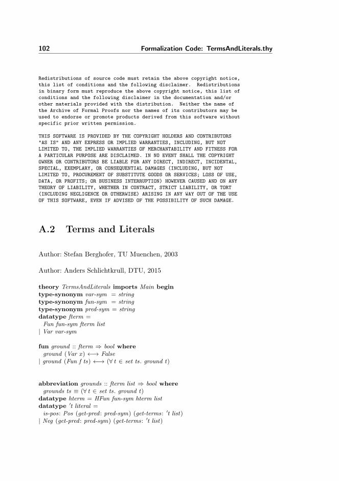
102 Formalization Code: TermsAndLiterals.thy
Redistributions of source code must retain the above copyright notice,this list of conditions and the following disclaimer. Redistributionsin binary form must reproduce the above copyright notice, this list ofconditions and the following disclaimer in the documentation and/orother materials provided with the distribution. Neither the name ofthe Archive of Formal Proofs nor the names of its contributors may beused to endorse or promote products derived from this software withoutspecific prior written permission.
THIS SOFTWARE IS PROVIDED BY THE COPYRIGHT HOLDERS AND CONTRIBUTORS"AS IS" AND ANY EXPRESS OR IMPLIED WARRANTIES, INCLUDING, BUT NOTLIMITED TO, THE IMPLIED WARRANTIES OF MERCHANTABILITY AND FITNESS FORA PARTICULAR PURPOSE ARE DISCLAIMED. IN NO EVENT SHALL THE COPYRIGHTOWNER OR CONTRIBUTORS BE LIABLE FOR ANY DIRECT, INDIRECT, INCIDENTAL,SPECIAL, EXEMPLARY, OR CONSEQUENTIAL DAMAGES (INCLUDING, BUT NOTLIMITED TO, PROCUREMENT OF SUBSTITUTE GOODS OR SERVICES; LOSS OF USE,DATA, OR PROFITS; OR BUSINESS INTERRUPTION) HOWEVER CAUSED AND ON ANYTHEORY OF LIABILITY, WHETHER IN CONTRACT, STRICT LIABILITY, OR TORT(INCLUDING NEGLIGENCE OR OTHERWISE) ARISING IN ANY WAY OUT OF THE USEOF THIS SOFTWARE, EVEN IF ADVISED OF THE POSSIBILITY OF SUCH DAMAGE.
A.2 Terms and Literals
Author: Stefan Berghofer, TU Muenchen, 2003
Author: Anders Schlichtkrull, DTU, 2015
theory TermsAndLiterals imports Main begintype-synonym var-sym = stringtype-synonym fun-sym = stringtype-synonym pred-sym = stringdatatype fterm =Fun fun-sym fterm list| Var var-sym
fun ground :: fterm ⇒ bool whereground (Var x ) ←→ False| ground (Fun f ts) ←→ (∀ t ∈ set ts. ground t)
abbreviation grounds :: fterm list ⇒ bool wheregrounds ts ≡ (∀ t ∈ set ts. ground t)
datatype hterm = HFun fun-sym hterm listdatatype ′t literal =is-pos: Pos (get-pred : pred-sym) (get-terms: ′t list)| Neg (get-pred : pred-sym) (get-terms: ′t list)
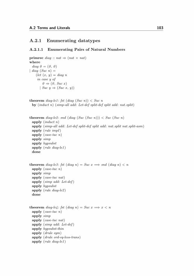
A.2 Terms and Literals 103
A.2.1 Enumerating datatypes
A.2.1.1 Enumerating Pairs of Natural Numbers
primrec diag :: nat ⇒ (nat × nat)wherediag 0 = (0 , 0 )| diag (Suc n) =
(let (x , y) = diag nin case y of
0 ⇒ (0 , Suc x )| Suc y ⇒ (Suc x , y))
theorem diag-le1 : fst (diag (Suc n)) < Suc nby (induct n) (simp-all add : Let-def split-def split add : nat .split)
theorem diag-le2 : snd (diag (Suc (Suc n))) < Suc (Suc n)apply (induct n)apply (simp-all add : Let-def split-def split add : nat .split nat .split-asm)apply (rule impI )apply (case-tac n)apply simpapply hypsubstapply (rule diag-le1 )done
theorem diag-le3 : fst (diag n) = Suc x =⇒ snd (diag n) < napply (case-tac n)apply simpapply (case-tac nat)apply (simp add : Let-def )apply hypsubstapply (rule diag-le2 )done
theorem diag-le4 : fst (diag n) = Suc x =⇒ x < napply (case-tac n)apply simpapply (case-tac nat)apply (simp add : Let-def )apply hypsubst-thinapply (drule sym)apply (drule ord-eq-less-trans)apply (rule diag-le1 )
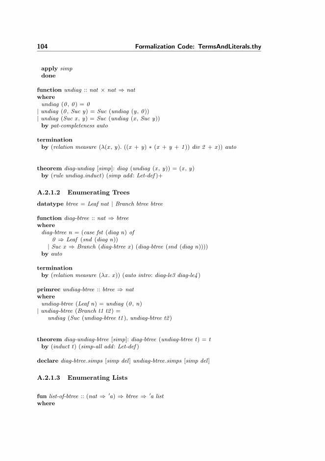
104 Formalization Code: TermsAndLiterals.thy
apply simpdone
function undiag :: nat × nat ⇒ natwhereundiag (0 , 0 ) = 0| undiag (0 , Suc y) = Suc (undiag (y , 0 ))| undiag (Suc x , y) = Suc (undiag (x , Suc y))by pat-completeness auto
terminationby (relation measure (λ(x , y). ((x + y) ∗ (x + y + 1 )) div 2 + x )) auto
theorem diag-undiag [simp]: diag (undiag (x , y)) = (x , y)by (rule undiag .induct) (simp add : Let-def )+
A.2.1.2 Enumerating Trees
datatype btree = Leaf nat | Branch btree btree
function diag-btree :: nat ⇒ btreewherediag-btree n = (case fst (diag n) of
0 ⇒ Leaf (snd (diag n))| Suc x ⇒ Branch (diag-btree x ) (diag-btree (snd (diag n))))
by auto
terminationby (relation measure (λx . x )) (auto intro: diag-le3 diag-le4 )
primrec undiag-btree :: btree ⇒ natwhereundiag-btree (Leaf n) = undiag (0 , n)| undiag-btree (Branch t1 t2 ) =
undiag (Suc (undiag-btree t1 ), undiag-btree t2 )
theorem diag-undiag-btree [simp]: diag-btree (undiag-btree t) = tby (induct t) (simp-all add : Let-def )
declare diag-btree.simps [simp del ] undiag-btree.simps [simp del ]
A.2.1.3 Enumerating Lists
fun list-of-btree :: (nat ⇒ ′a) ⇒ btree ⇒ ′a listwhere

A.2 Terms and Literals 105
list-of-btree f (Leaf x ) = []| list-of-btree f (Branch (Leaf n) t) = f n # list-of-btree f t
primrec btree-of-list :: ( ′a ⇒ nat) ⇒ ′a list ⇒ btreewherebtree-of-list f [] = Leaf 0| btree-of-list f (x # xs) = Branch (Leaf (f x )) (btree-of-list f xs)
definition diag-list :: (nat ⇒ ′a) ⇒ nat ⇒ ′a list wherediag-list f n = list-of-btree f (diag-btree n)
definition undiag-list :: ( ′a ⇒ nat) ⇒ ′a list ⇒ nat whereundiag-list f xs = undiag-btree (btree-of-list f xs)
theorem diag-undiag-list [simp]:(∧x . d (u x ) = x ) =⇒ diag-list d (undiag-list u xs) = xs
by (induct xs) (simp-all add : diag-list-def undiag-list-def )
A.2.1.4 Enumerating hterms
fun term-of-btree :: (nat ⇒ string) ⇒ btree ⇒ htermand term-list-of-btree :: (nat ⇒ string) ⇒ btree ⇒ hterm listwhereterm-of-btree f (Leaf m) = HFun (f m) []| term-of-btree f (Branch (Leaf m) t) =
HFun (f m) (term-list-of-btree f t)| term-list-of-btree f (Leaf m) = []| term-list-of-btree f (Branch t1 t2 ) =
term-of-btree f t1 # term-list-of-btree f t2
primrec btree-of-term :: (string ⇒ nat) ⇒ hterm ⇒ btreeand btree-of-term-list :: (string ⇒ nat) ⇒ hterm list ⇒ btree
wherebtree-of-term f (HFun m ts) = (if ts=[] then Leaf (f m) else Branch (Leaf (f m))
(btree-of-term-list f ts))| btree-of-term-list f [] = Leaf 0| btree-of-term-list f (t # ts) = Branch (btree-of-term f t) (btree-of-term-list f ts)
theorem term-btree: assumes du:∧x . d (u x ) = x
shows term-of-btree d (btree-of-term u t) = tand term-list-of-btree d (btree-of-term-list u ts) = tsby (induct t and ts rule: btree-of-term.induct btree-of-term-list .induct) (simp-all
add : du)
106 Formalization Code: TermsAndLiterals.thy
definition diag-term :: (nat ⇒ string) ⇒ nat ⇒ hterm wherediag-term f n = term-of-btree f (diag-btree n)
definition undiag-term :: (string ⇒ nat) ⇒ hterm ⇒ nat whereundiag-term f t = undiag-btree (btree-of-term f t)
theorem diag-undiag-term [simp]:(∧x . d (u x ) = x ) =⇒ diag-term d (undiag-term u t) = t
by (simp add : diag-term-def undiag-term-def term-btree)
A.2.1.5 Enumerating chars
definition diag-char :: nat ⇒ char wherediag-char == char-of-nat
definition undiag-char :: char ⇒ nat whereundiag-char == nat-of-char
theorem diag-undiag-char [simp]: diag-char (undiag-char c) = cunfolding diag-char-def undiag-char-def by auto
A.2.1.6 Enumerating strings
definition diag-string :: nat ⇒ string wherediag-string ≡ diag-list diag-char
definition undiag-string :: string ⇒ nat whereundiag-string ≡ undiag-list undiag-char
theorem diag-undiag-string [simp]:diag-string (undiag-string s) = sunfolding diag-string-def undiag-string-def by auto
A.2.1.7 Really enumerating hterms
definition diag-hterm :: nat ⇒ hterm wherediag-hterm ≡ diag-term diag-string
A.2 Terms and Literals 107
definition undiag-hterm :: hterm ⇒ nat whereundiag-hterm ≡ undiag-term undiag-string
theorem diag-undiag-hterm[simp]:diag-hterm (undiag-hterm t) = tunfolding diag-hterm-def undiag-hterm-def by auto
A.2.1.8 Enumerating hatoms
definition undiag-hatom :: hterm literal ⇒ nat whereundiag-hatom a ≡ undiag (undiag-string (get-pred a), undiag-list undiag-hterm
(get-terms a))
definition diag-hatom :: nat ⇒ hterm literal wherediag-hatom a ≡
(let (p,ts) = diag a in(Pos (diag-string p) (diag-list diag-hterm ts))
)
theorem diag-undiag-hatom[simp]:is-pos a =⇒ diag-hatom (undiag-hatom a) = aunfolding diag-hatom-def undiag-hatom-def by auto
A.2.1.9 Enumerating ground terms
primrec fterm-of-hterm :: hterm ⇒ ftermand fterms-of-hterms :: hterm list ⇒ fterm list wherefterm-of-hterm (HFun p ts) = Fun p (fterms-of-hterms ts)| fterms-of-hterms [] = []| fterms-of-hterms (t#ts) = fterm-of-hterm t # fterms-of-hterms tsprimrec hterm-of-fterm :: fterm ⇒ htermand hterms-of-fterms :: fterm list ⇒ hterm list wherehterm-of-fterm (Fun p ts) = HFun p (hterms-of-fterms ts)| hterms-of-fterms [] = []| hterms-of-fterms (t#ts) = hterm-of-fterm t # hterms-of-fterms ts
theorem [simp]: hterm-of-fterm (fterm-of-hterm t) = thterms-of-fterms (fterms-of-hterms ts) = ts
by (induct t and ts rule: fterm-of-hterm.induct fterms-of-hterms.induct) auto
theorem [simp]: ground t =⇒ fterm-of-hterm (hterm-of-fterm t) = tgrounds ts =⇒fterms-of-hterms (hterms-of-fterms ts) = ts
by (induct t and ts rule: hterm-of-fterm.induct hterms-of-fterms.induct) auto
108 Formalization Code: TermsAndLiterals.thy
definition diag-fterm :: nat ⇒ fterm wherediag-fterm n = fterm-of-hterm (diag-hterm n)
definition undiag-fterm :: fterm ⇒ nat whereundiag-fterm t = undiag-hterm (hterm-of-fterm t)
theorem diag-undiag-fterm: ground t =⇒ diag-fterm (undiag-fterm t) = tunfolding diag-fterm-def undiag-fterm-def by auto
A.2.1.10 Enumerating ground atoms
fun fatom-of-hatom :: hterm literal ⇒ fterm literal wherefatom-of-hatom (Pos p ts) = Pos p (fterms-of-hterms ts)| fatom-of-hatom (Neg p ts) = Neg p (fterms-of-hterms ts)
fun hatom-of-fatom :: fterm literal ⇒ hterm literal wherehatom-of-fatom (Pos p ts) = Pos p (hterms-of-fterms ts)| hatom-of-fatom (Neg p ts) = Neg p (hterms-of-fterms ts)
theorem [simp]: hatom-of-fatom (fatom-of-hatom (Pos p ts)) = Pos p tsby auto
theorem [simp]: grounds ts =⇒ fatom-of-hatom (hatom-of-fatom (Pos p ts)) = Posp tsby auto
definition undiag-fatom :: fterm literal ⇒ nat whereundiag-fatom t = undiag-hatom (hatom-of-fatom t)
definition diag-fatom :: nat ⇒ fterm literal wherediag-fatom n = fatom-of-hatom (diag-hatom n)
theorem diag-undiag-fatom[simp]: grounds ts =⇒ diag-fatom (undiag-fatom (Pos pts)) = Pos p tsunfolding undiag-fatom-def diag-fatom-def by auto
end

Appendix BFormalization Code:
Tree.thy
theory Tree imports Main begin
hide-const (open) Left Righttype-synonym dir = bool
definition Left :: bool where Left = True
definition Right :: bool where Right = Falsedeclare Left-def [simp]declare Right-def [simp]datatype tree =Leaf| Branch (ltree: tree) (rtree: tree)
B.1 Paths
inductive path :: dir list ⇒ tree ⇒ bool wherepath [] t| path ds l =⇒ path (Left#ds) (Branch l r)| path ds r =⇒ path (Right#ds) (Branch l r)
110 Formalization Code: Tree.thy
lemma path-inv-Leaf : path p Leaf ←→ p = []apply autousing path.simps apply blastapply (simp add : path.intros)done
lemma path-inv-Branch-Left :path (Left#p) (Branch l r) ←→ path p l
using path.intros apply autousing Left-def Right-def path.cases apply blastdone
lemma path-inv-Branch-Right :path (Right#p) (Branch l r) ←→ path p r
using path.intros apply autousing Left-def Right-def path.cases apply blastdone
lemma path-inv-Branch:path p (Branch l r) ←→ (p=[] ∨ (∃ a p ′. p=a#p ′∧ (a −→ path p ′ l) ∧ (¬a −→ path
p ′ r))) (is ?L ←→ ?R)proofassume ?L then show ?R using path.simps[of p] by auto
nextassume r : ?Rthen show ?Lproofassume p = [] then show ?L using path.intros by auto
nextassume ∃ a p ′. p=a#p ′∧ (a −→ path p ′ l) ∧ (¬a −→ path p ′ r)then obtain a p ′ where p=a#p ′∧ (a −→ path p ′ l) ∧ (¬a −→ path p ′ r) by
autothen show ?L using path.intros by (cases a) auto
qedqed
B.2 Branches
inductive branch :: dir list ⇒ tree ⇒ bool wherebranch [] Leaf| branch ds l =⇒ branch (Left # ds) (Branch l r)
B.2 Branches 111
| branch ds r =⇒ branch (Right # ds) (Branch l r)
lemma has-branch: ∃ b. branch b Tproof (induction T )case (Leaf ) then show ?case using branch.intros by auto
nextcase (Branch T 1 T 2)then obtain b where branch b T 1 by autothen have branch (Left#b) (Branch T 1 T 2) using branch.intros by autothen show ?case by auto
qed
lemma branch-inv-Leaf : branch b Leaf ←→ b = [] using branch.simps by blast
lemma branch-inv-Branch-Left :branch (Left#b) (Branch l r) ←→ branch b l
using branch.intros apply autousing Left-def Right-def branch.cases apply blastdone
lemma branch-inv-Branch-Right :branch (Right#b) (Branch l r) ←→ branch b r
using branch.intros apply autousing Left-def branch.cases by blast
lemma branch-inv-Branch:branch b (Branch l r) ←→
(∃ a b ′. b=a#b ′∧ (a −→ branch b ′ l) ∧ (¬a −→ branch b ′ r))using branch.simps[of b] by auto
lemma branch-inv-Leaf2 :T=Leaf ←→ (∀ b. branch b T −→ b=[])
proof −{assume T=Leafthen have ∀ b. branch b T −→ b = [] using branch-inv-Leaf by auto
}moreover{assume ∀ b. branch b T −→ b=[]then have ∀ b. branch b T −→ ¬(∃ a b ′. b = a # b ′) by autothen have ∀ b. branch b T −→ ¬(∃ l r . branch b (Branch l r))
112 Formalization Code: Tree.thy
using branch-inv-Branch by autothen have T=Leaf using has-branch[of T ] by (metis branch.simps)
}ultimately show T=Leaf ←→ (∀ b. branch b T −→ b=[]) by auto
qed
lemma branch-is-path:branch ds T =⇒ path ds T
proof (induction T arbitrary : ds)case Leafthen have ds = [] using branch-inv-Leaf by autothen show ?case using path.intros by auto
nextcase (Branch T 1 T 2)then obtain a b where ds-p: ds = a # b ∧ (a −→ branch b T 1) ∧ (¬ a −→ branch
b T 2) using branch-inv-Branch[of ds] by blastthen have (a −→ path b T 1) ∧ (¬a −→ path b T 2) using Branch by autothen show ?case using ds-p path.intros by (cases a) auto
qed
B.3 Internal Nodes
inductive internal :: dir list ⇒ tree ⇒ bool whereinternal [] (Branch l r)| internal ds l =⇒ internal (Left#ds) (Branch l r)| internal ds r =⇒ internal (Right#ds) (Branch l r)
lemma internal-inv-Leaf : ¬internal b Leaf using internal .simps by blast
lemma internal-inv-Branch-Left :internal (Left#b) (Branch l r) ←→ internal b l
apply ruleusing internal .intros apply autousing Left-def Right-def internal .cases apply blastdone
lemma internal-inv-Branch-Right :internal (Right#b) (Branch l r) ←→ internal b r
using internal .intros apply autousing Left-def Right-def internal .cases apply blastdone

B.3 Internal Nodes 113
lemma internal-inv-Branch:internal p (Branch l r) ←→ (p=[] ∨ (∃ a p ′. p=a#p ′∧ (a −→ internal p ′ l) ∧ (¬a−→ internal p ′ r))) (is ?L ←→ ?R)proofassume ?L then show ?R using internal .simps[of p] by auto
nextassume r : ?Rthen show ?Lproofassume p = [] then show ?L using internal .intros by auto
nextassume ∃ a p ′. p=a#p ′∧ (a −→ internal p ′ l) ∧ (¬a −→ internal p ′ r)then obtain a p ′ where p=a#p ′∧ (a −→ internal p ′ l) ∧ (¬a −→ internal p ′
r) by autothen show ?L using internal .intros by (cases a) auto
qedqed
lemma internal-is-path:internal ds T =⇒ path ds T
proof (induction T arbitrary : ds)case Leafthen have False using internal-inv-Leaf by autothen show ?case by auto
nextcase (Branch T 1 T 2)then obtain a b where ds-p: ds=[] ∨ ds = a # b ∧ (a −→ internal b T 1) ∧ (¬ a−→ internal b T 2) using internal-inv-Branch by blastthen have ds = [] ∨ (a −→ path b T 1) ∧ (¬a −→ path b T 2) using Branch by
autothen show ?case using ds-p path.intros by (cases a) auto
qed
fun parent :: dir list ⇒ dir list whereparent ds = tl ds
abbreviation prefix :: ′a list ⇒ ′a list ⇒ bool whereprefix a b ≡ ∃ c. a @ c = b
abbreviation pprefix :: ′a list ⇒ ′a list ⇒ bool wherepprefix a b ≡ ∃ c. a @ c = b ∧ a 6=b
114 Formalization Code: Tree.thy
abbreviation postfix :: ′a list ⇒ ′a list ⇒ bool wherepostfix a b ≡ ∃ c. c @ a = b
abbreviation ppostfix :: ′a list ⇒ ′a list ⇒ bool whereppostfix a b ≡ ∃ c. c @ a = b ∧ a 6=b
B.4 Deleting Nodes
fun delete :: dir list ⇒ tree ⇒ tree wheredelete [] T = Leaf| delete (True#ds) (Branch T 1 T 2) = Branch (delete ds T 1) T 2
| delete (False#ds) (Branch T 1 T 2) = Branch T 1 (delete ds T 2)
fun cutoff :: (dir list ⇒ bool) ⇒ dir list ⇒ tree ⇒ tree wherecutoff red ds (Branch T 1 T 2) =(if red ds then Leaf else Branch (cutoff red (ds@[Left ]) T 1) (cutoff red (ds@[Right ])
T 2))| cutoff red ds Leaf = Leaf
abbreviation anypath :: tree ⇒ (dir list ⇒ bool) ⇒ bool whereanypath T P ≡ ∀ p. path p T −→ P p
abbreviation anybranch :: tree ⇒ (dir list ⇒ bool) ⇒ bool whereanybranch T P ≡ ∀ p. branch p T −→ P p
abbreviation anyinternal :: tree ⇒ (dir list ⇒ bool) ⇒ bool whereanyinternal T P ≡ ∀ p. internal p T −→ P p
lemma cutoff-branch ′:anybranch T (λb. red(ds@b)) =⇒ anybranch (cutoff red ds T ) (λb. red(ds@b))
proof (induction T arbitrary : ds)case (Leaf )let ?T = cutoff red ds Leaf{fix bassume branch b ?T

B.4 Deleting Nodes 115
then have branch b Leaf by autothen have red(ds@b) using Leaf by auto
}then show ?case by simp
nextcase (Branch T 1 T 2)let ?T = cutoff red ds (Branch T 1 T 2)from Branch have ∀ p. branch (Left#p) (Branch T 1 T 2) −→ red (ds @ (Left#p))
by blastthen have ∀ p. branch p T 1 −→ red (ds @ (Left#p)) using branch.intros by autothen have anybranch T 1 (λp. red ((ds @ [Left ]) @ p)) using branch.intros by
autothen have aa: anybranch (cutoff red (ds @ [Left ]) T 1) (λp. red ((ds @ [Left ]) @
p))using Branch by blast
from Branch have ∀ p. branch (Right#p) (Branch T 1 T 2) −→ red (ds @ (Right#p))by blastthen have ∀ p. branch p T 2 −→ red (ds @ (Right#p)) using branch.intros by autothen have anybranch T 2 (λp. red ((ds @ [Right ]) @ p)) using branch.intros by
autothen have bb: anybranch (cutoff red (ds @ [Right ]) T 2) (λp. red ((ds @ [Right ]) @
p))using Branch by blast
{fix bassume b-p: branch b ?Thave red ds ∨ ¬red ds by autothen have red(ds@b)proofassume ds-p: red dsthen have ?T = Leaf by autothen have b = [] using b-p branch-inv-Leaf by autothen show red(ds@b) using ds-p by auto
nextassume ds-p: ¬red dslet ?T 1
′ = cutoff red (ds@[Left ]) T 1
let ?T 2′ = cutoff red (ds@[Right ]) T 2
from ds-p have ?T = Branch ?T 1′ ?T 2
′ by autofrom this b-p obtain a b ′ where b = a # b ′ ∧ (a −→ branch b ′ ?T 1
′) ∧ (¬a−→ branch b ′ ?T 2
′ ) using branch-inv-Branch[of b ?T 1′ ?T 2
′] by autothen show red(ds@b) using aa bb by (cases a) auto
qed}then show ?case by blast
qed
116 Formalization Code: Tree.thy
lemma cutoff-branch: anybranch T (λp. red p) =⇒ anybranch (cutoff red [] T ) (λp.red p)using cutoff-branch ′[of T red []] by auto
lemma cutoff-internal ′:anybranch T (λb. red(ds@b)) =⇒ anyinternal (cutoff red ds T ) (λb. ¬red(ds@b))
proof (induction T arbitrary : ds)case (Leaf ) then show ?case using internal-inv-Leaf by simp
nextcase (Branch T 1 T 2)let ?T = cutoff red ds (Branch T 1 T 2)from Branch have ∀ p. branch (Left#p) (Branch T 1 T 2) −→ red (ds @ (Left#p))
by blastthen have ∀ p. branch p T 1 −→ red (ds @ (Left#p)) using branch.intros by autothen have anybranch T 1 (λp. red ((ds @ [Left ]) @ p)) using branch.intros by
autothen have aa: anyinternal (cutoff red (ds @ [Left ]) T 1) (λp. ¬ red ((ds @ [Left ])
@ p)) using Branch by blast
from Branch have ∀ p. branch (Right#p) (Branch T 1 T 2) −→ red (ds @ (Right#p))by blastthen have ∀ p. branch p T 2 −→ red (ds @ (Right#p)) using branch.intros by autothen have anybranch T 2 (λp. red ((ds @ [Right ]) @ p)) using branch.intros by
autothen have bb: anyinternal (cutoff red (ds @ [Right ]) T 2) (λp. ¬ red ((ds @ [Right ])
@ p)) using Branch by blast{fix passume b-p: internal p ?Tthen have ds-p: ¬red ds using internal-inv-Leaf internal .intros by autohave p=[] ∨ p 6=[] by autothen have ¬red(ds@p)proofassume p=[] then show ¬red(ds@p) using ds-p by auto
nextlet ?T 1
′ = cutoff red (ds@[Left ]) T 1
let ?T 2′ = cutoff red (ds@[Right ]) T 2
assume p 6=[]moreoverhave ?T = Branch ?T 1
′ ?T 2′ using ds-p by auto
ultimatelyobtain a p ′ where b-p: p = a # p ′ ∧
(a −→ internal p ′ (cutoff red (ds @ [Left ]) T 1)) ∧(¬ a −→ internal p ′ (cutoff red (ds @ [Right ]) T 2))
using b-p internal-inv-Branch[of p ?T 1′ ?T 2
′] by auto
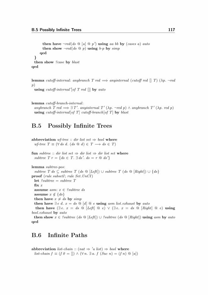
B.5 Possibly Infinite Trees 117
then have ¬red(ds @ [a] @ p ′) using aa bb by (cases a) autothen show ¬red(ds @ p) using b-p by simp
qed}then show ?case by blast
qed
lemma cutoff-internal : anybranch T red =⇒ anyinternal (cutoff red [] T ) (λp. ¬redp)using cutoff-internal ′[of T red []] by auto
lemma cutoff-branch-internal :anybranch T red =⇒ ∃T ′. anyinternal T ′ (λp. ¬red p) ∧ anybranch T ′ (λp. red p)using cutoff-internal [of T ] cutoff-branch[of T ] by blast
B.5 Possibly Infinite Trees
abbreviation wf-tree :: dir list set ⇒ bool wherewf-tree T ≡ (∀ ds d . (ds @ d) ∈ T −→ ds ∈ T )
fun subtree :: dir list set ⇒ dir list ⇒ dir list set wheresubtree T r = {ds ∈ T . ∃ ds ′. ds = r @ ds ′}
lemma subtree-pos:subtree T ds ⊆ subtree T (ds @ [Left ]) ∪ subtree T (ds @ [Right ]) ∪ {ds}
proof (rule subsetI ; rule Set .UnCI )let ?subtree = subtree Tfix xassume asm: x ∈ ?subtree dsassume x /∈ {ds}then have x 6= ds by simpthen have ∃ e d . x = ds @ [d ] @ e using asm list .exhaust by autothen have (∃ e. x = ds @ [Left ] @ e) ∨ (∃ e. x = ds @ [Right ] @ e) using
bool .exhaust by autothen show x ∈ ?subtree (ds @ [Left ]) ∪ ?subtree (ds @ [Right ]) using asm by auto
qed
B.6 Infinite Paths
abbreviation list-chain :: (nat ⇒ ′a list) ⇒ bool wherelist-chain f ≡ (f 0 = []) ∧ (∀n. ∃ a. f (Suc n) = (f n) @ [a])

118 Formalization Code: Tree.thy
lemma chain-length: list-chain f =⇒ length (f n) = napply (induction n)apply autoapply (metis length-append-singleton)done
lemma chain-prefix : list-chain f =⇒ n1 ≤ n2 =⇒ ∃ a. (f n1) @ a = (f n2)proof (induction n2)case (Suc n2)then have n1 ≤ n2 ∨ n1 = Suc n2 by autothen show ?caseproofassume n1 ≤ n2
then obtain a where a: f n1 @ a = f n2 using Suc by autohave b: ∃ b. f (Suc n2) = f n2 @ [b] using Suc by autofrom a b have ∃ b. f n1 @ (a @ [b]) = f (Suc n2) by autothen show ∃ c. f n1 @ c = f (Suc n2) by blast
nextassume n1 = Suc n2
then have f n1 @ [] = f (Suc n2) by autothen show ∃ a. f n1 @ a = f (Suc n2) by auto
qedqed auto
lemma ith-in-extension:assumes chain: list-chain fassumes smalli : i < length (f n1)assumes n1n2: n1 ≤ n2
shows f n1 ! i = f n2 ! iproof −from chain n1n2 have ∃ a. f n1 @ a = f n2 using chain-prefix by blastthen obtain a where a-p: f n1 @ a = f n2 by autohave (f n1 @ a) ! i = f n1 ! i using smalli by (simp add : nth-append)then show ?thesis using a-p by auto
qed
B.7 König’s Lemma
lemma inf-subs:assumes inf : ¬finite(subtree T ds)shows ¬finite(subtree T (ds @ [Left ])) ∨ ¬finite(subtree T (ds @ [Right ]))
proof −let ?subtree = subtree T
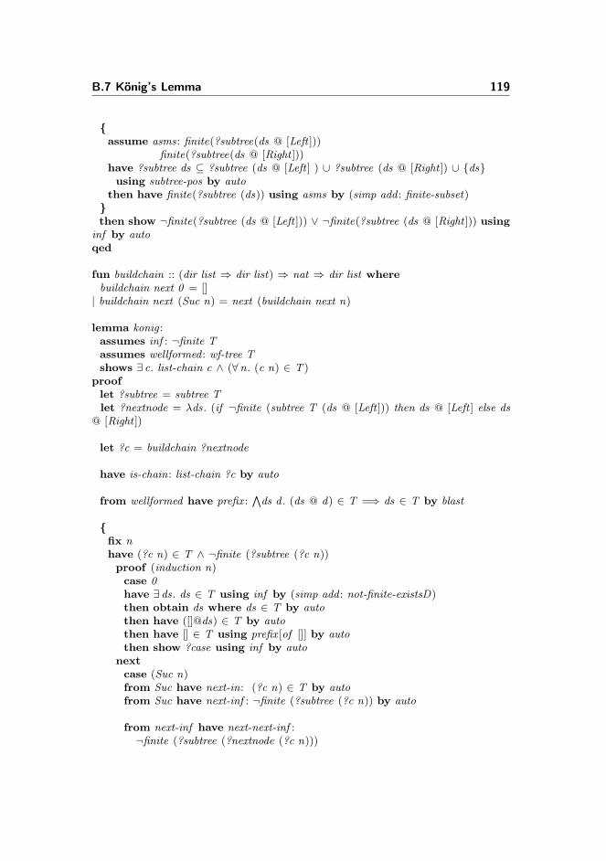
B.7 König’s Lemma 119
{assume asms: finite(?subtree(ds @ [Left ]))
finite(?subtree(ds @ [Right ]))have ?subtree ds ⊆ ?subtree (ds @ [Left ] ) ∪ ?subtree (ds @ [Right ]) ∪ {ds}using subtree-pos by auto
then have finite(?subtree (ds)) using asms by (simp add : finite-subset)}then show ¬finite(?subtree (ds @ [Left ])) ∨ ¬finite(?subtree (ds @ [Right ])) using
inf by autoqed
fun buildchain :: (dir list ⇒ dir list) ⇒ nat ⇒ dir list wherebuildchain next 0 = []| buildchain next (Suc n) = next (buildchain next n)
lemma konig :assumes inf : ¬finite Tassumes wellformed : wf-tree Tshows ∃ c. list-chain c ∧ (∀n. (c n) ∈ T )
prooflet ?subtree = subtree Tlet ?nextnode = λds. (if ¬finite (subtree T (ds @ [Left ])) then ds @ [Left ] else ds
@ [Right ])
let ?c = buildchain ?nextnode
have is-chain: list-chain ?c by auto
from wellformed have prefix :∧ds d . (ds @ d) ∈ T =⇒ ds ∈ T by blast
{fix nhave (?c n) ∈ T ∧ ¬finite (?subtree (?c n))proof (induction n)case 0have ∃ ds. ds ∈ T using inf by (simp add : not-finite-existsD)then obtain ds where ds ∈ T by autothen have ([]@ds) ∈ T by autothen have [] ∈ T using prefix [of []] by autothen show ?case using inf by auto
nextcase (Suc n)from Suc have next-in: (?c n) ∈ T by autofrom Suc have next-inf : ¬finite (?subtree (?c n)) by auto
from next-inf have next-next-inf :¬finite (?subtree (?nextnode (?c n)))
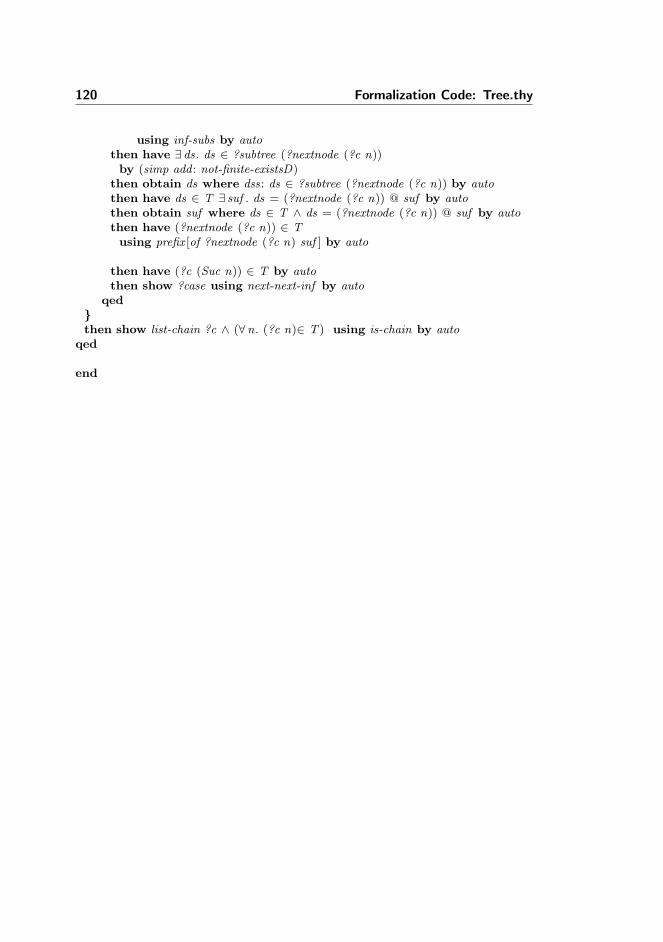
120 Formalization Code: Tree.thy
using inf-subs by autothen have ∃ ds. ds ∈ ?subtree (?nextnode (?c n))by (simp add : not-finite-existsD)
then obtain ds where dss: ds ∈ ?subtree (?nextnode (?c n)) by autothen have ds ∈ T ∃ suf . ds = (?nextnode (?c n)) @ suf by autothen obtain suf where ds ∈ T ∧ ds = (?nextnode (?c n)) @ suf by autothen have (?nextnode (?c n)) ∈ Tusing prefix [of ?nextnode (?c n) suf ] by auto
then have (?c (Suc n)) ∈ T by autothen show ?case using next-next-inf by auto
qed}then show list-chain ?c ∧ (∀n. (?c n)∈ T ) using is-chain by auto
qed
end
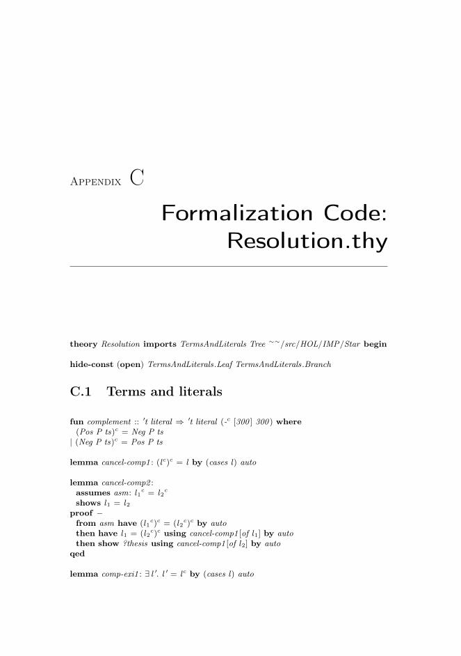
Appendix CFormalization Code:
Resolution.thy
theory Resolution imports TermsAndLiterals Tree ∼∼/src/HOL/IMP/Star begin
hide-const (open) TermsAndLiterals.Leaf TermsAndLiterals.Branch
C.1 Terms and literals
fun complement :: ′t literal ⇒ ′t literal (-c [300 ] 300 ) where(Pos P ts)c = Neg P ts| (Neg P ts)c = Pos P ts
lemma cancel-comp1 : (lc)c = l by (cases l) auto
lemma cancel-comp2 :assumes asm: l1c = l2c
shows l1 = l2proof −from asm have (l1c)c = (l2c)c by autothen have l1 = (l2c)c using cancel-comp1 [of l1] by autothen show ?thesis using cancel-comp1 [of l2] by auto
qed
lemma comp-exi1 : ∃ l ′. l ′ = lc by (cases l) auto
122 Formalization Code: Resolution.thy
lemma comp-exi2 : ∃ l . l ′ = lc
proofshow l ′ = (l ′c)c using cancel-comp1 [of l ′] by auto
qed
lemma comp-swap: l1c = l2 ←→ l1 = l2c
proof −have l1c = l2 =⇒ l1 = l2c using cancel-comp1 [of l1] by automoreoverhave l1 = l2c =⇒ l1c = l2 using cancel-comp1 by autoultimatelyshow ?thesis by auto
qed
C.2 Clausestype-synonym ′t clause = ′t literal set
abbreviation complementls :: ′t literal set ⇒ ′t literal set (-C [300 ] 300 ) whereLC ≡ complement ‘ L
lemma cancel-compls1 : (LC)C = Lapply autoapply (simp add : cancel-comp1 )apply (metis imageI cancel-comp1 )done
lemma cancel-compls2 :assumes asm: L1
C = L2C
shows L1 = L2
proof −from asm have (L1
C)C = (L2C)C by auto
then show ?thesis using cancel-compls1 [of L1] cancel-compls1 [of L2] by simpqed
fun varst :: fterm ⇒ var-sym setand varsts :: fterm list ⇒ var-sym set wherevarst (Var x ) = {x}| varst (Fun f ts) = varsts ts| varsts [] = {}| varsts (t # ts) = (varst t) ∪ (varsts ts)
definition varsl :: fterm literal ⇒ var-sym set wherevarsl l = varsts (get-terms l)
definition varsls :: fterm literal set ⇒ var-sym set where
C.3 Semantics 123
varsls L ≡⋃l∈L. varsl l
abbreviation groundl :: fterm literal ⇒ bool wheregroundl l ≡ grounds (get-terms l)
abbreviation groundls :: fterm clause ⇒ bool wheregroundls L ≡ ∀ l ∈ L. groundl l
lemma ground-comp: groundl (lc) ←→ groundl l by (cases l) auto
lemma ground-compls: groundls (LC) ←→ groundls L using ground-comp by auto
C.3 Semanticstype-synonym ′u fun-denot = fun-sym ⇒ ′u list ⇒ ′utype-synonym ′u pred-denot = pred-sym ⇒ ′u list ⇒ booltype-synonym ′u var-denot = var-sym ⇒ ′u
fun evalt :: ′u var-denot ⇒ ′u fun-denot ⇒ fterm ⇒ ′u whereevalt E F (Var x ) = E x| evalt E F (Fun f ts) = F f (map (evalt E F ) ts)
abbreviation evalts :: ′u var-denot ⇒ ′u fun-denot ⇒ fterm list ⇒ ′u list whereevalts E F ts ≡ map (evalt E F ) ts
fun evall :: ′u var-denot ⇒ ′u fun-denot ⇒ ′u pred-denot ⇒ fterm literal ⇒ boolwhereevall E F G (Pos p ts) ←→ (G p (evalts E F ts))| evall E F G (Neg p ts) ←→ ¬(G p (evalts E F ts))
definition evalc :: ′u fun-denot ⇒ ′u pred-denot ⇒ fterm clause ⇒ bool whereevalc F G C ←→ (∀E . ∃ l ∈ C . evall E F G l)
definition evalcs :: ′u fun-denot ⇒ ′u pred-denot ⇒ fterm clause set ⇒ bool whereevalcs F G Cs ←→ (∀C ∈ Cs. evalc F G C )
definition validcs :: fterm clause set ⇒ bool wherevalidcs Cs ←→ (∀F G. evalcs F G Cs)
C.3.1 Semantics of Ground Terms
lemma ground-var-denott : ground t =⇒ (evalt E F t = evalt E ′ F t)proof (induction t)case (Var x )then have False by autothen show ?case by auto

124 Formalization Code: Resolution.thy
nextcase (Fun f ts)then have ∀ t ∈ set ts. ground t by autothen have ∀ t ∈ set ts. evalt E F t = evalt E ′ F t using Fun by autothen have evalts E F ts = evalts E ′ F ts by autothen have F f (map (evalt E F ) ts) = F f (map (evalt E ′ F ) ts) by metisthen show ?case by simp
qed
lemma ground-var-denotts: grounds ts =⇒ (evalts E F ts = evalts E ′ F ts)using ground-var-denott by (metis map-eq-conv)
lemma ground-var-denot : groundl l =⇒ (evall E F G l = evall E ′ F G l)proof (induction l)case Pos then show ?case using ground-var-denotts by (metis evall .simps(1 )
literal .sel(3 ))nextcase Neg then show ?case using ground-var-denotts by (metis evall .simps(2 )
literal .sel(4 ))qed
C.4 Substitutionstype-synonym substitution = var-sym ⇒ fterm
fun sub :: fterm ⇒ substitution ⇒ fterm (-{-}t [300 ,0 ] 300 ) where(Var x ){σ}t = σ x| (Fun f ts){σ}t = Fun f (map (λt . t {σ}t) ts)
abbreviation subs :: fterm list ⇒ substitution ⇒ fterm list (-{-}ts [300 ,0 ] 300 )wherets{σ}ts ≡ (map (λt . t {σ}t) ts)
fun subl :: fterm literal ⇒ substitution ⇒ fterm literal (-{-}l [300 ,0 ] 300 ) where(Pos p ts){σ}l = Pos p (ts{σ}ts)| (Neg p ts){σ}l = Neg p (ts{σ}ts)
abbreviation subls :: fterm literal set ⇒ substitution ⇒ fterm literal set (-{-}ls[300 ,0 ] 300 ) whereL {σ}ls ≡ (λl . l {σ}l) ‘ L
definition instance-oft :: fterm ⇒ fterm ⇒ bool whereinstance-oft t1 t2 ←→ (∃σ. t1 = t2{σ}t)
definition instance-ofts :: fterm list ⇒ fterm list ⇒ bool whereinstance-ofts ts1 ts2 ←→ (∃σ. ts1 = ts2{σ}ts)
C.4 Substitutions 125
definition instance-ofl :: fterm literal ⇒ fterm literal ⇒ bool whereinstance-ofl l1 l2 ←→ (∃σ. l1 = l2{σ}l)
lemma comp-sub: (lc) {σ}l=(l {σ}l)cby (cases l) auto
definition var-renaming :: substitution ⇒ bool wherevar-renaming σ ←→ (∀ x . ∃ y . σ x = Var y)
C.4.1 The Empty Substitution
abbreviation ε :: substitution whereε ≡ Var
lemma empty-subt : (t :: fterm){ε}t = tapply (induction t)apply (auto simp add : map-idI )done
lemma empty-subts: (ts :: fterm list){ε}ts = tsusing empty-subt by auto
lemma empty-subl : (l :: fterm literal){ε}l = lusing empty-subts by (cases l) auto
lemma instance-oft-self : instance-oft t tunfolding instance-oft-defproofshow t = t{ε}t using empty-subt by auto
qed
lemma instance-ofts-self : instance-ofts ts tsunfolding instance-ofts-defproofshow ts = ts{ε}ts using empty-subts by auto
qed
lemma instance-ofl-self : instance-ofl l lunfolding instance-ofl-defproofshow l = l{ε}l using empty-subl by auto
qed
C.4.2 Substitutions and Ground Terms
lemma ground-sub: ground t =⇒ t {σ}t = t
126 Formalization Code: Resolution.thy
apply (induction t)apply (auto simp add : map-idI )done
lemma ground-subs: grounds ts =⇒ ts {σ}ts = tsusing ground-sub by (simp add : map-idI )
lemma groundl-subs: groundl l =⇒ l {σ}l = lusing ground-subs by (cases l) auto
lemma groundls-subls:assumes ground : groundls Lshows L {σ}ls = L
proof −{fix lassume l-L: l ∈ Lthen have groundl l using ground by autothen have l = l{σ}l using groundl-subs by automoreoverthen have l {σ}l ∈ L {σ}ls using l-L by autoultimatelyhave l ∈ L {σ}ls by auto
}moreover{fix lassume l-L: l ∈ L {σ}lsthen obtain l ′ where l ′-p: l ′ ∈ L ∧ l ′ {σ}l = l by autothen have l ′ = l using ground groundl-subs by autofrom l-L l ′-p this have l ∈ L by auto
}ultimately show ?thesis by auto
qed
C.4.3 Composition
definition composition :: substitution ⇒ substitution ⇒ substitution (infixl · 55 )where(σ1 · σ2) x = (σ1 x ){σ2}t
lemma composition-conseq2t : t{σ1}t{σ2}t = t{σ1 · σ2}tproof (induction t)case (Var x )have (Var x ){σ1}t{σ2}t = (σ1 x ){σ2}t by simpalso have ... = (σ1 · σ2) x unfolding composition-def by simpfinally show ?case by auto

C.4 Substitutions 127
nextcase (Fun t ts)then show ?case unfolding composition-def by auto
qed
lemma composition-conseq2ts: ts{σ1}ts{σ2}ts = ts{σ1 · σ2}tsusing composition-conseq2t by auto
lemma composition-conseq2l : l{σ1}l{σ2}l = l{σ1 · σ2}lusing composition-conseq2t by (cases l) auto
lemma composition-assoc: σ1 · (σ2 · σ3) = (σ1 · σ2) · σ3
prooffix xshow (σ1 · (σ2 · σ3)) x = ((σ1 · σ2) · σ3) x unfolding composition-def using
composition-conseq2t by simpqed
lemma empty-comp1 : (σ · ε) = σprooffix xshow (σ · ε) x = σ x unfolding composition-def using empty-subt by auto
qed
lemma empty-comp2 : (ε · σ) = σprooffix xshow (ε · σ) x = σ x unfolding composition-def by simp
qed
lemma instance-ofts-trans :assumes ts12: instance-ofts ts1 ts2assumes ts23: instance-ofts ts2 ts3shows instance-ofts ts1 ts3
proof −from ts12 obtain σ12 where ts1 = ts2 {σ12}tsunfolding instance-ofts-def by auto
moreoverfrom ts23 obtain σ23 where ts2 = ts3 {σ23}tsunfolding instance-ofts-def by auto
ultimatelyhave ts1 = ts3 {σ23}ts {σ12}ts by autothen have ts1 = ts3 {σ23 · σ12}ts using composition-conseq2ts by simpthen show ?thesis unfolding instance-ofts-def by auto
qed

128 Formalization Code: Resolution.thy
C.5 Unifiers
definition unifiert :: substitution ⇒ fterm set ⇒ bool whereunifiert σ ts ←→ (∃ t ′. ∀ t ∈ ts. t{σ}t = t ′)
definition unifierls :: substitution ⇒ fterm literal set ⇒ bool whereunifierls σ L ←→ (∃ l ′. ∀ l ∈ L. l{σ}l = l ′)
lemma unif-sub:assumes unif : unifierls σ Lassumes nonempty : L 6= {}shows ∃ l . subls L σ = {subl l σ}
proof −from nonempty obtain l where l ∈ L by autofrom unif this have L {σ}ls = {l {σ}l} unfolding unifierls-def by autothen show ?thesis by auto
qed
lemma unifierls-def2 :assumes L-elem: L 6= {}shows unifierls σ L ←→ (∃ l . L {σ}ls ={l})
proofassume unif : unifierls σ Lfrom L-elem obtain l where l ∈ L by autothen have L {σ}ls = {l {σ}l} using unif unfolding unifierls-def by autothen show ∃ l . L{σ}ls = {l} by auto
nextassume ∃ l . L {σ}ls ={l}then obtain l where L {σ}ls = {l} by autothen have ∀ l ′ ∈ L. l ′{σ}l = l by autothen show unifierls σ L unfolding unifierls-def by auto
qed
lemma groundls-unif-singleton:assumes groundls: groundls Lassumes unif : unifierls σ ′ Lassumes empt : L 6= {}shows ∃ l . L = {l}
proof −from unif empt have ∃ l . L {σ ′}ls = {l} using unif-sub by autothen show ?thesis using groundls-subls groundls by auto
qed
definition unifiablet :: fterm set ⇒ bool whereunifiablet fs ←→ (∃σ. unifiert σ fs)

C.5 Unifiers 129
definition unifiablels :: fterm literal set ⇒ bool whereunifiablels L ←→ (∃σ. unifierls σ L)
lemma unifier-comp[simp]: unifierls σ (LC) ←→ unifierls σ Lproofassume unifierls σ (LC)then obtain l ′′ where l ′′-p: ∀ l ∈ LC . l{σ}l = l ′′
unfolding unifierls-def by autoobtain l ′ where (l ′)c = l ′′ using comp-exi2 [of l ′′] by autofrom this l ′′-p have l ′-p:∀ l ∈ LC . l{σ}l = (l ′)c by autohave ∀ l ∈ L. l{σ}l = l ′
prooffix lassume l∈Lthen have lc ∈ LC by autothen have (lc){σ}l = (l ′)c using l ′-p by autothen have (l {σ}l)c = (l ′)c by (cases l) autothen show l{σ}l = l ′ using cancel-comp2 by blast
qedthen show unifierls σ L unfolding unifierls-def by auto
nextassume unifierls σ Lthen obtain l ′ where l ′-p: ∀ l ∈ L. l{σ}l = l ′ unfolding unifierls-def by autohave ∀ l ∈ LC . l{σ}l = (l ′)c
prooffix lassume l ∈ LC
then have lc ∈ L using cancel-comp1 by (metis image-iff )then show l{σ}l = (l ′)c using l ′-p comp-sub cancel-comp1 by metis
qedthen show unifierls σ (LC) unfolding unifierls-def by auto
qed
lemma unifier-sub1 : unifierls σ L =⇒ L ′ ⊆ L =⇒ unifierls σ L ′
unfolding unifierls-def by auto
lemma unifier-sub2 :assumes asm: unifierls σ (L1 ∪ L2)shows unifierls σ L1 ∧ unifierls σ L2
proof −have L1 ⊆ (L1 ∪ L2) ∧ L2 ⊆ (L1 ∪ L2) by simpfrom this asm show ?thesis using unifier-sub1 by auto
qed
C.5.1 Most General Unifiers
130 Formalization Code: Resolution.thy
definition mgut :: substitution ⇒ fterm set ⇒ bool wheremgut σ fs ←→ unifiert σ fs ∧ (∀ u. unifiert u fs −→ (∃ i . u = σ · i))
definition mguls :: substitution ⇒ fterm literal set ⇒ bool wheremguls σ L ←→ unifierls σ L ∧ (∀ u. unifierls u L −→ (∃ i . u = σ · i))
C.6 Resolution
definition applicable :: fterm clause ⇒ fterm clause⇒ fterm literal set ⇒ fterm literal set⇒ substitution ⇒ bool where
applicable C 1 C 2 L1 L2 σ ←→C 1 6= {} ∧ C 2 6= {} ∧ L1 6= {} ∧ L2 6= {}∧ varsls C 1 ∩ varsls C 2 = {}∧ L1 ⊆ C 1 ∧ L2 ⊆ C 2
∧ mguls σ (L1 ∪ L2C)
definition resolution :: fterm clause ⇒ fterm clause⇒ fterm literal set ⇒ fterm literal set⇒ substitution ⇒ fterm clause where
resolution C 1 C 2 L1 L2 σ = (C 1 {σ}ls − L1 {σ}ls) ∪ (C 2 {σ}ls − L2 {σ}ls)
inductive resolution-step :: fterm clause set ⇒ fterm clause set ⇒ bool whereresolution-rule:C 1 ∈ Cs =⇒ C 2 ∈ Cs =⇒ applicable C 1 C 2 L1 L2 σ =⇒
resolution-step Cs (Cs ∪ {resolution C 1 C 2 L1 L2 σ})| standardize-apart :
C ∈ Cs =⇒ var-renaming σ =⇒ resolution-step Cs (Cs ∪ {C {σ}ls})
definition resolution-deriv :: fterm clause set ⇒ fterm clause set ⇒ bool whereresolution-deriv = star resolution-step
lemma ground-resolution:assumes ground : groundls C 1 ∧ groundls C 2
assumes appl : applicable C 1 C 2 L1 L2 σshows resolution C 1 C 2 L1 L2 σ = (C 1 − L1) ∪ (C 2 − L2) ∧ (∃ l . L1 = {l} ∧ L2
= {l}C)proof −from appl ground have groundl : groundls L1 ∧ groundls L2 unfolding applicable-defby autofrom this ground appl have resl : (C 1 {σ}ls − L1 {σ}ls) ∪ (C 2 {σ}ls − L2 {σ}ls)
= (C 1 − L1) ∪ (C 2 − L2)using groundls-subls unfolding applicable-def by auto
from ground appl have l1 ′l2 ′ground : groundls L1 ∧ groundls L2
unfolding applicable-def by auto
C.7 Soundness 131
then have groundls (L1 ∪ L2C) using ground-compls by auto
moreoverfrom appl have unifierls σ (L1 ∪ L2
C) unfolding mguls-def applicable-def by autoultimatelyobtain l where L1 ∪ L2
C = {l}using appl groundls-unif-singletonunfolding applicable-def by (metis sup-eq-bot-iff )from appl this have L1 = {l} ∧ L2
C = {l} unfolding applicable-def by (metisimage-is-empty singleton-Un-iff )then have l-p: L1 = {l} ∧ L2 = {l}C using cancel-compls1 [of L2] by auto
from resl l-p show ?thesis unfolding resolution-def by autoqed
lemma ground-resolution-ground :assumes asm: groundls C 1 ∧ groundls C 2
assumes appl : applicable C 1 C 2 L1 L2 σshows groundls (resolution C 1 C 2 L1 L2 σ)
proof −from asm appl have resolution C 1 C 2 L1 L2 σ = (C 1 − L1) ∪ (C 2 − L2) using
ground-resolution by autothen show ?thesis using asm by auto
qed
C.7 Soundness
fun evalsub :: ′u fun-denot ⇒ ′u var-denot ⇒ substitution ⇒ ′u var-denot whereevalsub F E σ = (evalt E F ) ◦ σ
lemma substitutiont : evalt E F (t {σ}t) = evalt (evalsub F E σ) F tapply (induction t)apply autoapply (metis (mono-tags, lifting) comp-apply map-cong)done
lemma substitutionts: evalts E F (ts {σ}ts) = evalts (evalsub F E σ) F tsusing substitutiont by auto
lemma substitutionl : evall E F G (l {σ}l) ←→ evall (evalsub F E σ) F G lapply (induction l)using substitutionts apply (metis evall .simps(1 ) subl .simps(1 ))using substitutionts apply (metis evall .simps(2 ) subl .simps(2 ))done
132 Formalization Code: Resolution.thy
lemma subst-sound :assumes asm: evalc F G Cshows evalc F G (C {σ}ls )
proof −have ∀E . ∃ l ∈ C {σ}ls. evall E F G lprooffix Efrom asm have ∃ l ∈ C . evall (evalsub F E σ) F G l unfolding evalc-def by
autothen show ∃ l ∈ C {σ}ls. evall E F G l using substitutionl [of E F G - σ] by
autoqed
then show ?thesis unfolding evalc-def by autoqed
lemma simple-resolution-sound :assumes C 1sat : evalc F G C 1
assumes C 2sat : evalc F G C 2
assumes l1inc1: l1 ∈ C 1
assumes l2inc2: l2 ∈ C 2
assumes Comp: l1c = l2shows evalc F G ((C 1 − {l1}) ∪ (C 2 − {l2}))
proof −have ∀E . ∃ l ∈ (((C 1 − {l1}) ∪ (C 2 − {l2}))). evall E F G lprooffix Ehave evall E F G l1 ∨ evall E F G l2 using Comp by (cases l1) autothen show ∃ l ∈ (((C 1 − {l1}) ∪ (C 2 − {l2}))). evall E F G lproofassume evall E F G l1then have ¬evall E F G l2 using Comp by (cases l1) auto
then have ∃ l2 ′∈ C 2. l2 ′ 6= l2 ∧ evall E F G l2 ′ using l2inc2 C 2sat unfoldingevalc-def by auto
then show ∃ l∈(C 1 − {l1}) ∪ (C 2 − {l2}). evall E F G l by autonextassume evall E F G l2then have ¬evall E F G l1 using Comp by (cases l1) auto
then have ∃ l1 ′∈ C 1. l1 ′ 6= l1 ∧ evall E F G l1 ′ using l1inc1 C 1sat unfoldingevalc-def by auto
then show ∃ l∈(C 1 − {l1}) ∪ (C 2 − {l2}). evall E F G l by autoqed
qedthen show ?thesis unfolding evalc-def by simp
qed
lemma resolution-sound :assumes sat1: evalc F G C 1

C.7 Soundness 133
assumes sat2: evalc F G C 2
assumes appl : applicable C 1 C 2 L1 L2 σshows evalc F G (resolution C 1 C 2 L1 L2 σ)
proof −from sat1 have sat1σ: evalc F G (C 1 {σ}ls) using subst-sound by blastfrom sat2 have sat2σ: evalc F G (C 2 {σ}ls) using subst-sound by blast
from appl obtain l1 where l1-p: l1 ∈ L1 unfolding applicable-def by auto
from l1-p appl have l1 ∈ C 1 unfolding applicable-def by autothen have inc1σ: l1 {σ}l ∈ C 1 {σ}ls by auto
from l1-p have unified1: l1 ∈ (L1 ∪ (L2C)) by auto
from l1-p appl have l1σisl1σ: {l1{σ}l} = L1 {σ}lsunfolding mguls-def unifierls-def applicable-def by auto
from appl obtain l2 where l2-p: l2 ∈ L2 unfolding applicable-def by auto
from l2-p appl have l2 ∈ C 2 unfolding applicable-def by autothen have inc2σ: l2 {σ}l ∈ C 2 {σ}ls by auto
from l2-p have unified2: l2c ∈ (L1 ∪ (L2C)) by auto
from unified1 unified2 appl have l1 {σ}l = (l2c){σ}lunfolding mguls-def unifierls-def applicable-def by auto
then have comp: (l1 {σ}l)c = l2 {σ}l using comp-sub comp-swap by auto
from appl have unifierls σ (L2C)
using unifier-sub2 unfolding mguls-def applicable-def by blastthen have unifierls σ L2 by autofrom this l2-p have l2σisl2σ: {l2{σ}l} = L2 {σ}ls unfolding unifierls-def by auto
from sat1σ sat2σ inc1σ inc2σ comp have evalc F G (C 1{σ}ls − {l1{σ}l} ∪(C 2{σ}ls − {l2{σ}l})) using simple-resolution-sound [of F G C 1 {σ}ls C 2 {σ}ls l1{σ}l l2 {σ}l]
by autofrom this l1σisl1σ l2σisl2σ show ?thesis unfolding resolution-def by auto
qed
lemma sound-step: resolution-step Cs Cs ′ =⇒ evalcs F G Cs =⇒ evalcs F G Cs ′
proof (induction rule: resolution-step.induct)case (resolution-rule C 1 Cs C 2 l1 l2 σ)then have evalc F G C 1 ∧ evalc F G C 2 unfolding evalcs-def by autothen have evalc F G (resolution C 1 C 2 l1 l2 σ)using resolution-sound resolution-rule by auto
then show ?case using resolution-rule unfolding evalcs-def by auto
134 Formalization Code: Resolution.thy
nextcase (standardize-apart C Cs σ)then have evalc F G C unfolding evalcs-def by autothen have evalc F G (C{σ}ls) using subst-sound by autothen show ?case using standardize-apart unfolding evalcs-def by auto
qed
lemma sound-derivation:resolution-deriv Cs Cs ′ =⇒ evalcs F G Cs =⇒ evalcs F G Cs ′
unfolding resolution-deriv-defproof (induction rule: star .induct)case refl then show ?case by auto
nextcase (step Cs1 Cs2 Cs3) then show ?case using sound-step by auto
qed
C.8 Enumerations
fun hlit-of-flit :: fterm literal ⇒ hterm literal wherehlit-of-flit (Pos P ts) = Pos P (hterms-of-fterms ts)| hlit-of-flit (Neg P ts) = Neg P (hterms-of-fterms ts)
lemma undiag-neg : undiag-fatom (Neg P ts) = undiag-fatom (Pos P ts)unfolding undiag-fatom-def undiag-hatom-def by auto
lemma undiag-neg2 : undiag-hatom (Neg P ts) = undiag-hatom (Pos P ts)unfolding undiag-fatom-def undiag-hatom-def by auto
lemma ground-h-undiag : groundl l =⇒ undiag-hatom (hlit-of-flit l) = undiag-fatom lproof (induction l)case (Pos P ts)then show ?case unfolding undiag-fatom-def by auto
nextcase (Neg P ts)then show ?case using undiag-neg undiag-neg2 unfolding undiag-fatom-def by
autoqed
C.9 Herbrand Interpretationsvalue HFun
C.10 Partial Interpretations 135
lemma hterms-ground : ground (fterm-of-hterm t) grounds (fterms-of-hterms ts)apply (induction t and ts rule: fterm-of-hterm.induct fterms-of-hterms.induct)apply autodone
lemma eval-ground : ground t =⇒ (evalt E HFun t) = hterm-of-fterm t grounds ts=⇒ (evalts E HFun ts) = hterms-of-fterms tsapply (induction t and ts rule: hterm-of-fterm.induct hterms-of-fterms.induct)apply autodone
lemma evall-grounds:assumes asm: grounds tsshows evall E HFun G (Pos P ts) ←→ G P (hterms-of-fterms ts)
proof −have evall E HFun G (Pos P ts) = G P (evalts E HFun ts) by autoalso have ... = G P (hterms-of-fterms ts) using asm eval-ground by metisfinally show ?thesis by auto
qed
C.10 Partial Interpretationstype-synonym partial-pred-denot = bool list
fun falsifiesl :: partial-pred-denot ⇒ fterm literal ⇒ bool wherefalsifiesl G (Pos p ts) =
(∃ i ts ′.i < length G∧ G ! i = False∧ diag-fatom i = Pos p ts ′
∧ instance-ofts ts ′ ts)| falsifiesl G (Neg p ts) =
(∃ i ts ′.i < length G∧ G ! i = True∧ diag-fatom i = Pos p ts ′
∧ instance-ofts ts ′ ts)
abbreviation falsifiesc :: partial-pred-denot ⇒ fterm clause ⇒ bool wherefalsifiesc G C ≡ (∀ l ∈ C . falsifiesl G l)
abbreviation falsifiescs :: partial-pred-denot ⇒ fterm clause set ⇒ bool wherefalsifiescs G Cs ≡ (∃C ∈ Cs. falsifiesc G C )
abbreviation extend :: (nat ⇒ partial-pred-denot) ⇒ hterm pred-denot where

136 Formalization Code: Resolution.thy
extend f P ts ≡ (let n = undiag-hatom (Pos P ts) inf (Suc n) ! n
)
fun sub-of-denot :: hterm var-denot ⇒ substitution wheresub-of-denot E = fterm-of-hterm ◦ E
lemma ground-sub-of-denott : ground ((t :: fterm) {sub-of-denot E}t)apply (induction t)apply (auto simp add : hterms-ground)done
lemma ground-sub-of-denotts: grounds ((ts :: fterm list) {sub-of-denot E}ts)apply autousing ground-sub-of-denott apply simpdone
lemma ground-sub-of-denotl : groundl ((l :: fterm literal) {sub-of-denot E}l)proof −have grounds (subs (get-terms l :: fterm list) (sub-of-denot E))using ground-sub-of-denotts by auto
then show ?thesis by (cases l) autoqed
lemma sub-of-denot-equivx : evalt E HFun (sub-of-denot E x ) = E xproof −have ground (sub-of-denot E x ) using hterms-ground by autothenhave evalt E HFun (sub-of-denot E x ) = hterm-of-fterm (sub-of-denot E x )using eval-ground(1 ) by auto
also have ... = hterm-of-fterm (fterm-of-hterm (E x )) by autoalso have ... = E x by autofinally show ?thesis by auto
qed
lemma sub-of-denot-equivt :evalt E HFun (t {sub-of-denot E}t) = evalt E HFun t
apply (induction t)using sub-of-denot-equivx apply autodone
lemma sub-of-denot-equivts: evalts E HFun (ts {sub-of-denot E}ts) = evalts E HFuntsusing sub-of-denot-equivt apply simpdone

C.10 Partial Interpretations 137
lemma sub-of-denot-equivl : evall E HFun G (l {sub-of-denot E}l) = evall E HFun Glproof (induction l)case (Pos p ts)have evall E HFun G ((Pos p ts) {sub-of-denot E}l) ←→ G p (evalts E HFun (ts{sub-of-denot E}ts)) by autoalso have ... ←→ G p (evalts E HFun ts) using sub-of-denot-equivts[of E ts] by
metisalso have ... ←→ evall E HFun G (Pos p ts) by simpfinallyshow ?case by blast
nextcase (Neg p ts)have evall E HFun G ((Neg p ts) {sub-of-denot E}l) ←→ ¬G p (evalts E HFun (ts{sub-of-denot E}ts)) by autoalso have ... ←→ ¬G p (evalts E HFun ts) using sub-of-denot-equivts[of E ts] by
metisalso have ... = evall E HFun G (Neg p ts) by simpfinallyshow ?case by blast
qed
lemma sub-of-denot-equiv-ground ′:evall E HFun G l = evall E HFun G (l {sub-of-denot E}l) ∧ groundl (l {sub-of-denot
E}l)using sub-of-denot-equivl ground-sub-of-denotl by auto
lemma partial-equiv-subst ′: falsifiesl G ((l ::fterm literal) {σ}l) =⇒ falsifiesl G lproof (induction l)case (Pos P ts)then have falsifiesl G (Pos P (ts{σ}ts)) by autothen obtain i ts ′ where i-ts ′:
i < length G∧ G ! i = False∧ diag-fatom i = Pos P ts ′
∧ instance-ofts ts ′ (ts {σ}ts) by automoreoverhave instance-ofts (ts {σ}ts) ts unfolding instance-ofts-def by autothen have instance-ofts ts ′ ts using i-ts ′ instance-ofts-trans by autoultimatelyhave
i < length G∧ G ! i = False∧ diag-fatom i = Pos P ts ′
∧ instance-ofts ts ′ ts by auto
138 Formalization Code: Resolution.thy
then show ?case by autonextcase (Neg P ts)then have falsifiesl G (Neg P (ts{σ}ts)) by autothen obtain i ts ′ where i-ts ′:
i < length G∧ G ! i = True∧ diag-fatom i = Pos P ts ′
∧ instance-ofts ts ′ (ts {σ}ts) by automoreoverhave instance-ofts (ts {σ}ts) ts unfolding instance-ofts-def by autothen have instance-ofts ts ′ ts using i-ts ′ instance-ofts-trans by autoultimatelyhave
i < length G∧ G ! i = True∧ diag-fatom i = Pos P ts ′
∧ instance-ofts ts ′ ts by autothen show ?case by auto
qed
lemma partial-equiv-subst :assumes asm: falsifiesc G ((C :: fterm clause) {σ}ls)shows falsifiesc G C
prooffix lassume l ∈ Cthen have falsifiesl G (l {σ}l) using asm by autothen show falsifiesl G l using partial-equiv-subst ′ by auto
qed
lemma sub-of-denot-equiv-ground :((∃ l ∈ C . evall E HFun G l) ←→ (∃ l ∈ C {sub-of-denot E}ls. evall E HFun G l))
∧ groundls (C {sub-of-denot E}ls)using sub-of-denot-equiv-ground ′ by auto
C.10.1 Semantic Trees
abbreviation closed-branch :: partial-pred-denot ⇒ tree ⇒ fterm clause set ⇒ boolwhereclosed-branch G T Cs ≡ branch G T ∧ falsifiescs G Cs
abbreviation open-branch :: partial-pred-denot ⇒ tree ⇒ fterm clause set ⇒ boolwhereopen-branch G T Cs ≡ branch G T ∧ ¬falsifiescs G Cs
C.11 Herbrand’s Theorem 139
fun closed-tree :: tree ⇒ fterm clause set ⇒ bool whereclosed-tree T Cs ←→ anybranch T (λb. closed-branch b T Cs)
∧ anyinternal T (λp. ¬falsifiescs p Cs)
C.11 Herbrand’s Theorem
lemma maximum:assumes asm: finite Cshows ∃n :: nat . ∀ l ∈ C . f l ≤ n
prooffrom asm show ∀ l∈C . f l ≤ (Max (f ‘ C )) by auto
qed
lemma extend-preserves-model :assumes f-chain: list-chain (f :: nat ⇒ partial-pred-denot)assumes n-max : ∀ l∈C . undiag-fatom l ≤ nassumes C-ground : groundls Cassumes C-false: ¬evalc HFun (extend f ) Cshows falsifiesc (f (Suc n)) C
prooflet ?F = HFunlet ?G = extend f
fix lassume asm: l∈Clet ?i = undiag-fatom lfrom asm have i-n: ?i ≤ n using n-max by autothen have j-n: ?i ≤ length (f n) using f-chain chain-length[of f n] by auto
from C-false have ¬(∀E . ∃ l ∈ C . evall E ?F ?G l) unfolding evalc-def by autothen have ∃E . ∀ l ∈ C . ¬ evall E ?F ?G l by autothen have ∀E . ∀ l ∈ C . ¬ evall E ?F ?G l using C-ground ground-var-denot by
blastthen have last : ∀E . ¬ evall E ?F ?G l using asm by blast
then show falsifiesl (f (Suc n)) lproof (cases l)case (Pos P ts)from Pos asm C-ground have ts-ground : grounds ts by autofrom Pos asm C-ground have undiag-l : undiag-hatom (hlit-of-flit l) = ?i using
ground-h-undiag by blast
from last have ¬?G P (hterms-of-fterms ts) using evall-grounds[of ts - ?G P ]ts-ground Pos by auto
then have f (Suc ?i) ! ?i = False using Pos undiag-l by auto
140 Formalization Code: Resolution.thy
moreoverhave f (Suc ?i) ! ?i = f (Suc n) ! ?iusing f-chain i-n j-n chain-length[of f ] ith-in-extension[of f ] by simp
ultimately have f (Suc n) ! ?i = False by autothen have?i < length (f (Suc n)) (∗ j-n ∗)∧ f (Suc n) ! ?i = False (∗last thing ∗)∧ diag-fatom ?i = Pos P ts (∗ by definition of ?i ∗)∧ instance-ofts ts tsusing
j-n ts-ground diag-undiag-fatom instance-ofts-self f-chain chain-length[of f ]Pos
by autothen show ?thesis using Pos by auto
nextcase (Neg P ts)from Neg asm C-ground have ts-ground : grounds ts by autofrom Neg asm C-ground have undiag-l : undiag-hatom (hlit-of-flit l) = ?i using
ground-h-undiag by blast
from last have ?G P (hterms-of-fterms ts) using evall-grounds[of ts - ?G P ]C-ground asm Neg by auto
then have f (Suc ?i) ! ?i = True using Neg undiag-neg undiag-lby (metis hatom-of-fatom.simps undiag-fatom-def )
moreoverhave f (Suc ?i) ! ?i = f (Suc n) ! ?iusing f-chain i-n j-n chain-length[of f ] ith-in-extension[of f ] by simp
ultimately have f (Suc n) ! ?i = True by autothen have?i < length (f (Suc n)) (∗ j-n ∗)∧ f (Suc n) ! ?i = True (∗last thing ∗)∧ diag-fatom ?i = Pos P ts (∗ by definition of ?i ∗)∧ instance-ofts ts tsusing j-n diag-undiag-fatom instance-ofts-self [of ts] f-chain chain-length[of f ]
Neg undiag-neg ts-groundby auto
then show ?thesis using Neg by autoqed
qed
lemma list-chain-model :assumes f-chain: list-chain (f :: nat ⇒ partial-pred-denot)assumes model-cs: ∀n. ¬falsifiescs (f n) Csassumes fin-cs: finite Csassumes fin-c: ∀C ∈ Cs. finite C
C.11 Herbrand’s Theorem 141
shows ∃G. evalcs HFun G Csprooflet ?F = HFunlet ?G = extend f
have ∀C E . (C ∈ Cs −→ (∃ l ∈ C . evall E ?F ?G l))proof (rule allI ; rule allI ; rule impI )fix Cfix Eassume asm: C ∈ Cslet ?σ = sub-of-denot Ehave groundcσ: groundls (C {?σ}ls) using sub-of-denot-equiv-ground by autofrom fin-c asm have finite (C {?σ}ls) by autothen obtain n where largest : ∀ l ∈ (C {?σ}ls). undiag-fatom l ≤ n using
maximum by blastfrom model-cs asm have ¬falsifiesc (f (Suc n)) C by autothen have model-c: ¬falsifiesc (f (Suc n)) (C {?σ}ls) using partial-equiv-subst
by blast
have evalc HFun ?G (C {?σ}ls)using groundcσ f-chain largest model-c
extend-preserves-model [of f C {?σ}ls n] by blastthen have ∀E . ∃ l ∈ (C {?σ}ls). evall E ?F ?G l unfolding evalc-def by autothen have ∃ l ∈ (C {?σ}ls). evall E ?F ?G l by autothen show ∃ l∈C . evall E ?F ?G l using sub-of-denot-equiv-ground by simp
qedthen have ∀C ∈ Cs. ∀E . ∃ l ∈ C . evall E ?F ?G l by autothen have ∀C ∈ Cs. evalc ?F ?G C unfolding evalc-def by autothen show evalcs ?F ?G Cs unfolding evalcs-def by auto
qed
fun deeptree :: nat ⇒ tree wheredeeptree 0 = Leaf| deeptree (Suc n) = Branch (deeptree n) (deeptree n)
thm extend-preserves-modelthm list-chain-model
lemma branch-length: branch b (deeptree n) =⇒ length b = nproof (induction n arbitrary : b)case 0 then show ?case using branch-inv-Leaf by auto
nextcase (Suc n)then have branch b (Branch (deeptree n) (deeptree n)) by auto

142 Formalization Code: Resolution.thy
then obtain a b ′where p: b=a#b ′∧ branch b ′ (deeptree n) using branch-inv-Branch[ofb] by blastthen have length b ′ = n using Suc by autothen show ?case using p by auto
qed
lemma infinity :assumes bij : ∀n :: nat . undiago (diago n) = nassumes all-tree: ∀n :: nat . (diago n) ∈ treeshows ¬finite tree
proof −from bij all-tree have ∀n. n = undiago (diago n) ∧ (diago n) ∈ tree by autothen have ∀n. ∃ ds. n = undiago ds ∧ ds ∈ tree by autothen have undiago ‘ tree = (UNIV :: nat set) by autothen have ¬finite treeby (metis finite-imageI infinite-UNIV-nat)then show ?thesis by auto
qed
lemma longer-falsifies ′:falsifiesl ds l =⇒ falsifiesl (ds@d) l
proof (induction l)case (Pos P ts)then obtain i ts ′ where i-ts ′:
i < length ds∧ ds ! i = False∧ diag-fatom i = Pos P ts ′
∧ instance-ofts ts ′ ts by automoreoverfrom i-ts ′ have i < length (ds@d) by automoreoverfrom i-ts ′ have (ds@d) ! i = False by (simp add : nth-append)ultimatelyhave
i < length (ds@d)∧ (ds@d) ! i = False∧ diag-fatom i = Pos P ts ′
∧ instance-ofts ts ′ ts by autothen show ?case by auto
nextcase (Neg P ts)then obtain i ts ′ where i-ts ′:
i < length ds∧ ds ! i = True∧ diag-fatom i = Pos P ts ′
∧ instance-ofts ts ′ ts by auto
C.11 Herbrand’s Theorem 143
moreoverfrom i-ts ′ have i < length (ds@d) by automoreoverfrom i-ts ′ have (ds@d) ! i = True by (simp add : nth-append)ultimatelyhave
i < length (ds@d)∧ (ds@d) ! i = True∧ diag-fatom i = Pos P ts ′
∧ instance-ofts ts ′ ts by autothen show ?case by auto
qed
lemma longer-falsifies:assumes asm: falsifiescs ds Csshows falsifiescs (ds @ d) Cs
proof −from asm obtain C where C-p: C ∈ Cs ∧ falsifiesc ds C by autothen have ∀ l ∈ C . falsifiesl ds l by autothen have ∀ l ∈ C . falsifiesl (ds@d) l using longer-falsifies ′ by autothen have falsifiesc (ds @ d) C by autothen show falsifiescs (ds @ d) Cs using C-p by auto
qed
theorem herbrand ′:assumes openb: ∀T . ∃G. open-branch G T Csassumes finite-cs: finite Cs ∀C∈Cs. finite Cshows ∃G. evalcs HFun G Cs
proof −
let ?tree = {G. ¬falsifiescs G Cs}let ?undiag = lengthlet ?diag = (λl . SOME b. open-branch b (deeptree l) Cs) :: nat ⇒ partial-pred-denot
from openb have diag-open: ∀ l . open-branch (?diag l) (deeptree l) Csusing someI-ex [of %b. open-branch b (deeptree -) Cs] by auto
then have ∀n. ?undiag (?diag n) = n using branch-length by automoreoverhave ∀n. (?diag n) ∈ ?tree using diag-open by autoultimatelyhave ¬finite ?tree using infinity [of - λn. SOME b. open-branch b (- n) Cs] by simp
moreoverhave ∀ ds d . ¬falsifiescs (ds @ d) Cs −→ ¬falsifiescs ds Csusing longer-falsifies[of Cs] by blast
then have (∀ ds d . ds @ d ∈ ?tree −→ ds ∈ ?tree) by auto

144 Formalization Code: Resolution.thy
ultimatelyhave ∃ c. list-chain c ∧ (∀n. c n ∈ ?tree) using konig [of ?tree] by blastthen have ∃G. list-chain G ∧ (∀n. ¬ falsifiescs (G n) Cs) by auto
then show ∃G. evalcs HFun G Cs using list-chain-model finite-cs by autoqed
theorem herbrand ′-contra:assumes finite-cs: finite Cs ∀C∈Cs. finite Cassumes unsat : ∀G. ¬evalcs HFun G Csshows ∃T . ∀G. branch G T −→ closed-branch G T Cs
proof −from finite-cs unsat have ∀T . ∃G. open-branch G T Cs =⇒ ∃G. evalcs HFun G
Cs using herbrand ′ by blastthen show ?thesis using unsat by blast
qed
theorem herbrand :assumes unsat : ∀G. ¬ evalcs HFun G Csassumes finite-cs: finite Cs ∀C∈Cs. finite Cshows ∃T . closed-tree T Cs
proof −from unsat finite-cs obtain T where anybranch T (λb. closed-branch b T Cs)
using herbrand ′-contra[of Cs] by blastthen have ∃T . anybranch T (λp. falsifiescs p Cs) ∧ anyinternal T (λp. ¬ falsifiescs
p Cs)using cutoff-branch-internal [of T (λp. falsifiescs p Cs)] by blast
then show ?thesis by autoqed
C.12 Lifting Lemma
lemma lifting :assumes appart : varsc c ∩ varsc d = {}assumes inst1: instance-ofc c ′ cassumes inst2: instance-ofc d ′ dassumes appl : applicable c ′ d ′ l ′ m ′ σshows ∃ l m τ . applicable c d l m τ ∧
instance-ofc (resolution c ′ d ′ l ′ m ′ σ) (resolution c d l m τ)oops
C.13 Completeness
lemma falsifiesc [] C =⇒ C = {}

C.13 Completeness 145
proof −{ fix lassume l ∈ Cmoreoverhave ¬falsifiesl [] l by (cases l) autoultimately have ¬falsifiesc [] C by auto
} then show falsifiesc [] C =⇒ C = {} by autoqed
theorem completeness ′:assumes finite-cs: finite Cs ∀C∈Cs. finite Cshows closed-tree T Cs =⇒ ∃Cs ′. resolution-deriv Cs Cs ′ ∧ {} ∈ Cs ′
proof (induction T arbitrary : Cs rule: Nat .measure-induct-rule[of size])fix T ::treefix Cs :: fterm clause setassume (
∧T ′ Cs. size T ′ < size T =⇒
closed-tree T ′ Cs =⇒ ∃Cs ′. resolution-deriv Cs Cs ′ ∧ {} ∈ Cs ′)assume closed-tree T Cshave True by autothen show ∃Cs ′. resolution-deriv Cs Cs ′ ∧ {} ∈ Cs ′ oops
theorem completeness:assumes finite-cs: finite Cs ∀C∈Cs. finite Cassumes unsat : ∀F G. ¬evalcs F G Csshows ∃Cs ′. resolution-deriv Cs Cs ′ ∧ {} ∈ Cs ′
oops
end

146 Formalization Code: Resolution.thy

Appendix D
Formalization Code:Examples.thy
theory Examples imports Resolution beginvalue Var ′′x ′′
value Fun ′′one ′′ []value Fun ′′mul ′′ [Var ′′y ′′,Var ′′y ′′]value Fun ′′add ′′ [Fun ′′mul ′′ [Var ′′y ′′,Var ′′y ′′], Fun ′′one ′′ []]value Pos ′′greater ′′ [Var ′′x ′′, Var ′′y ′′]value Neg ′′less ′′ [Var ′′x ′′, Var ′′y ′′]value Pos ′′less ′′ [Var ′′x ′′, Var ′′y ′′]value Pos ′′equals ′′
[Fun ′′add ′′[Fun ′′mul ′′[Var ′′y ′′,Var ′′y ′′], Fun ′′one ′′[]],Var ′′x ′′]
fun Fnat :: nat fun-denot whereFnat f [n,m] =(if f = ′′add ′′ then n + m elseif f = ′′mul ′′ then n ∗ m else 0 )
| Fnat f [] =(if f = ′′one ′′ then 1 elseif f = ′′zero ′′ then 0 else 0 )
| Fnat f us = 0
fun Gnat :: nat pred-denot whereGnat p [x ,y ] =
(if p = ′′less ′′ ∧ x < y then True else

148 Formalization Code: Examples.thy
if p = ′′greater ′′ ∧ x > y then True elseif p = ′′equals ′′ ∧ x = y then True else False)
| Gnat p us = False
fun Enat :: nat var-denot whereEnat x =
(if x = ′′x ′′ then 26 elseif x = ′′y ′′ then 5 else 0 )
lemma evalt Enat Fnat (Var ′′x ′′) = 26by auto
lemma evalt Enat Fnat (Fun ′′one ′′ []) = 1by auto
lemma evalt Enat Fnat (Fun ′′mul ′′ [Var ′′y ′′,Var ′′y ′′]) = 25by auto
lemmaevalt Enat Fnat (Fun ′′add ′′ [Fun ′′mul ′′ [Var ′′y ′′,Var ′′y ′′], Fun ′′one ′′ []]) = 26by auto
lemma evall Enat Fnat Gnat (Pos ′′greater ′′ [Var ′′x ′′, Var ′′y ′′]) = Trueby auto
lemma evall Enat Fnat Gnat (Neg ′′less ′′ [Var ′′x ′′, Var ′′y ′′]) = Trueby auto
lemma evall Enat Fnat Gnat (Pos ′′less ′′ [Var ′′x ′′, Var ′′y ′′]) = Falseby auto
lemma evall Enat Fnat Gnat
(Pos ′′equals ′′
[Fun ′′add ′′ [Fun ′′mul ′′ [Var ′′y ′′,Var ′′y ′′],Fun ′′one ′′ []],Var ′′x ′′]
) = Trueby auto
definition PP :: fterm literal wherePP = Pos ′′P ′′ [Fun ′′c ′′ []]
definition PQ :: fterm literal wherePQ = Pos ′′Q ′′ [Fun ′′d ′′ []]
definition NP :: fterm literal where
149
NP = Neg ′′P ′′ [Fun ′′c ′′ []]
definition NQ :: fterm literal whereNQ = Neg ′′Q ′′ [Fun ′′d ′′ []]
theorem empty-mgu: unifierls ε L =⇒ mguls ε Lunfolding unifierls-def mguls-def apply autoapply (rule-tac x=u in exI )using empty-comp1 empty-comp2 apply (auto)done
theorem unifier-single: unifierls σ {l}unfolding unifierls-def by auto
theorem resolution-rule ′:C 1 ∈ Cs =⇒ C 2 ∈ Cs =⇒ applicable C 1 C 2 L1 L2 σ
=⇒ C = {resolution C 1 C 2 L1 L2 σ}=⇒ resolution-step Cs (Cs ∪ C )using resolution-rule by auto
lemma resolution-example1 :∃Cs. resolution-deriv {{NP ,PQ},{NQ},{PP ,PQ}}
{{NP ,PQ},{NQ},{PP ,PQ},{NP},{PP},{}}proof −have resolution-step
{{NP ,PQ},{NQ},{PP ,PQ}}({{NP ,PQ},{NQ},{PP ,PQ}} ∪ {{NP}})
apply (rule resolution-rule ′[of {NP ,PQ} - {NQ} {PQ} {NQ} ε])unfolding applicable-def varsls-def varsl-def
NQ-def NP-def PQ-def PP-def resolution-defusing unifier-single empty-mgu apply (auto)done
then have resolution-step{{NP ,PQ},{NQ},{PP ,PQ}}({{NP ,PQ},{NQ},{PP ,PQ},{NP}})
by (simp add : insert-commute)moreoverhave resolution-step
{{NP ,PQ},{NQ},{PP ,PQ},{NP}}({{NP ,PQ},{NQ},{PP ,PQ},{NP}} ∪ {{PP}})
apply (rule resolution-rule ′[of {NQ} - {PP ,PQ} {NQ} {PQ} ε])unfolding applicable-def varsls-def varsl-def
NQ-def NP-def PQ-def PP-def resolution-defusing unifier-single empty-mgu apply (auto)done
then have resolution-step
150 Formalization Code: Examples.thy
{{NP ,PQ},{NQ},{PP ,PQ},{NP}}({{NP ,PQ},{NQ},{PP ,PQ},{NP},{PP}})
by (simp add : insert-commute)moreoverhave resolution-step
{{NP ,PQ},{NQ},{PP ,PQ},{NP},{PP}}({{NP ,PQ},{NQ},{PP ,PQ},{NP},{PP}} ∪ {{}})
apply (rule resolution-rule ′[of {NP} - {PP} {NP} {PP} ε])unfolding applicable-def varsls-def varsl-def
NQ-def NP-def PQ-def PP-def resolution-defusing unifier-single empty-mgu apply (auto)done
then have resolution-step{{NP ,PQ},{NQ},{PP ,PQ},{NP},{PP}}({{NP ,PQ},{NQ},{PP ,PQ},{NP},{PP},{}})
by (simp add : insert-commute)ultimatelyhave resolution-deriv {{NP ,PQ},{NQ},{PP ,PQ}}
{{NP ,PQ},{NQ},{PP ,PQ},{NP},{PP},{}}unfolding resolution-deriv-def using star .intros[of resolution-step] by auto
then show ?thesis by autoqed
definition Pa :: fterm literal wherePa = Pos ′′a ′′ []
definition Na :: fterm literal whereNa = Neg ′′a ′′ []
definition Pb :: fterm literal wherePb = Pos ′′b ′′ []
definition Nb :: fterm literal whereNb = Neg ′′b ′′ []
definition Paa :: fterm literal wherePaa = Pos ′′a ′′ [Fun ′′a ′′ []]
definition Naa :: fterm literal whereNaa = Neg ′′a ′′ [Fun ′′a ′′ []]

151
definition Pax :: fterm literal wherePax = Pos ′′a ′′ [Var ′′x ′′]
definition Nax :: fterm literal whereNax = Neg ′′a ′′ [Var ′′x ′′]
definition mguPaaPax :: substitution wheremguPaaPax = (λx . if x = ′′x ′′ then Fun ′′a ′′ [] else Var x )
lemma mguPaaPax-mgu: mguls mguPaaPax {Paa,Pax}proof −let ?σ = λx . if x = ′′x ′′ then Fun ′′a ′′ [] else Var xhave a: unifierls (λx . if x = ′′x ′′ then Fun ′′a ′′ [] else Var x ) {Paa,Pax} unfolding
Paa-def Pax-def unifierls-def by autohave b: ∀ u. unifierls u {Paa,Pax} −→ (∃ i . u = ?σ · i)proof (rule;rule)fix uassume unifierls u {Paa,Pax}then have uuu: u ′′x ′′ = Fun ′′a ′′ [] unfolding unifierls-def Paa-def Pax-def
by autohave ?σ · u = uprooffix x{assume x= ′′x ′′
moreoverhave (?σ · u) ′′x ′′ = Fun ′′a ′′ [] unfolding composition-def by autoultimately have (?σ · u) x = u x using uuu by auto
}moreover{assume x 6= ′′x ′′then have (?σ · u) x = (ε x ) {u}t unfolding composition-def by autothen have (?σ · u) x = u x by auto
}ultimately show (?σ · u) x = u x by auto
qedthen have (∃ i . ?σ · i = u) by autothen show (∃ i . u = ?σ · i) by autoqed
from a b show ?thesis unfolding mguls-def unfolding mguPaaPax-def by autoqed
lemma resolution-example2 :∃Cs. resolution-deriv {{Nb,Na},{Pax},{Pa},{Na,Pb,Naa}}
152 Formalization Code: Examples.thy
{{Nb,Na},{Pax},{Pa},{Na,Pb,Naa},{Na,Pb},{Na},{}}proof −have resolution-step
{{Nb,Na},{Pax},{Pa},{Na,Pb,Naa}}({{Nb,Na},{Pax},{Pa},{Na,Pb,Naa}} ∪ {{Na,Pb}})
apply (rule resolution-rule ′[of {Pax} - {Na,Pb,Naa} {Pax} {Naa} mguPaaPax])
using mguPaaPax-mgu unfolding applicable-def varsls-def varsl-defNb-def Na-def Pax-def Pa-def Pb-def Naa-def Paa-def mguPaaPax-def
resolution-defapply autodone
then have resolution-step{{Nb,Na},{Pax},{Pa},{Na,Pb,Naa}}({{Nb,Na},{Pax},{Pa},{Na,Pb,Naa},{Na,Pb}})
by (simp add : insert-commute)moreoverhave resolution-step
{{Nb,Na},{Pax},{Pa},{Na,Pb,Naa},{Na,Pb}}({{Nb,Na},{Pax},{Pa},{Na,Pb,Naa},{Na,Pb}} ∪ {{Na}})
apply (rule resolution-rule ′[of {Nb,Na} - {Na,Pb} {Nb} {Pb} ε])unfolding applicable-def varsls-def varsl-def
Pb-def Nb-def Na-def PP-def resolution-defusing unifier-single empty-mgu apply (auto)done
then have resolution-step{{Nb,Na},{Pax},{Pa},{Na,Pb,Naa},{Na,Pb}}({{Nb,Na},{Pax},{Pa},{Na,Pb,Naa},{Na,Pb},{Na}})
by (simp add : insert-commute)moreoverhave resolution-step
{{Nb,Na},{Pax},{Pa},{Na,Pb,Naa},{Na,Pb},{Na}}({{Nb,Na},{Pax},{Pa},{Na,Pb,Naa},{Na,Pb},{Na}} ∪ {{}})
apply (rule resolution-rule ′[of {Na} - {Pa} {Na} {Pa} ε])unfolding applicable-def varsls-def varsl-def
Pa-def Nb-def Na-def PP-def resolution-defusing unifier-single empty-mgu apply (auto)done
then have resolution-step{{Nb,Na},{Pax},{Pa},{Na,Pb,Naa},{Na,Pb},{Na}}({{Nb,Na},{Pax},{Pa},{Na,Pb,Naa},{Na,Pb},{Na},{}})
by (simp add : insert-commute)ultimatelyhave resolution-deriv {{Nb,Na},{Pax},{Pa},{Na,Pb,Naa}}
{{Nb,Na},{Pax},{Pa},{Na,Pb,Naa},{Na,Pb},{Na},{}}unfolding resolution-deriv-def using star .intros[of resolution-step] by auto
then show ?thesis by auto
153
qed
lemma ref-sound :assumes deriv : resolution-deriv Cs Cs ′ ∧ {} ∈ Cs ′
shows ¬evalcs F G Csproof −from deriv have evalcs F G Cs =⇒ evalcs F G Cs ′ using sound-derivation by
automoreoverfrom deriv have evalcs F G Cs ′ =⇒ evalc F G {} unfolding evalcs-def by automoreoverthen have evalc F G {} =⇒ False unfolding evalc-def by autoultimately show ?thesis by auto
qed
lemma resolution-example1-sem: ¬evalcs F G {{NP , PQ}, {NQ}, {PP , PQ}}using resolution-example1 ref-sound by auto
lemma resolution-example2-sem: ¬evalcs F G {{Nb,Na},{Pax},{Pa},{Na,Pb,Naa}}using resolution-example2 ref-sound by auto
end

154 Formalization Code: Examples.thy

Appendix EChang and Lee’s Lifting
Lemma
Here follows an account of flaws and imprecisions in Chang and Lee’s proofof the lifting lemma [CL73]. It also presents a counter-example to the proof.Their notation uses ∼ to give the complement literal and ◦ for composition ofsubstitutions. Like Ben-Ari, they represent substitutions as finite sets of key-value pairs and can thus apply the ∪ operator to combine them.
Lemma 5.1 (Lifting Lemma) If C ′1 and C ′2 are instances of C1 and C2,respectively, and if C ′ is a resolvent of C ′1 and C ′2, then there is a resolventC of C1 and C2 such that C ′ is an instance of C.
Proof We rename, if necessary, the variables in C1 and C2 so that variablesin C1 are all different from those in C2. Let L′1 and L′2 be the literalsresolved upon, and let
C ′ = (C ′1γ − L′1γ) ∪ (C ′2γ − L′2γ),
where γ is a most general unifier of L′1 and ∼L′2.
This is problematic in the binary resolution with factoring of their book. Thereason is that in the proof it is assumed that no factoring is done on C ′1 and C ′2,

156 Chang and Lee’s Lifting Lemma
but factoring is actually allowed by the resolution calculus of the book. Onecould argue that it is acceptable, since factoring is just further instantiation andthus we could perhaps just obtain the factored C ′1 and C ′2. However, we will seein the counter-example that this handling of factors is problematic.
Since C ′1 and C ′2 are instances of C1 and C2, respectively, there is a substi-tution θ such that C ′1 = C1θ and C ′2 = C2θ. Let L1
i , ..., Lrii be the literals
in Ci corresponding to L′i (i.e., L1i θ = · · · = Lri
i θ = L′i), i = 1, 2. If ri > 1,obtain a most general unifier λi, for {L1
i , ..., Lrii } and let Li = L1
iλi, i = l, 2.(Note that L1
iλi, ..., Lrii λi are the same, since λi is a most general unifier.)
Then Li, is a literal in the factor Ciλi of Ci. If ri = 1, let λi = ε andLi = L1
iλi.
Let λ = λ1 ∪ λ2.
Like in the proof of Ben-Ari, we should make sure that the union λ1 ∪ λ2 iswell-formed. Again we could require additional properties of the mgus λ1 andλ2.
Thus, clearly L′i is an instance of Li. Since L′i and ∼L′2 are unifiable, L1
and ∼L2 are unifiable.
L′i should probably have been L′1 in the last sentence.
Let σ be a most general unifier of L1 and ∼L2. Let
C = ((C1λ)σ − L1σ) ∪ ((C2λ)σ − L2σ)
= ((C1λ)σ − ({L11, ..., L
r11 }λ)σ) ∪ ((C2λ)σ − ({L1
2, ..., Lr22 }λ)σ)
= (C1(λ ◦ σ)− {L11, ..., L
r11 }(λ ◦ σ)) ∪ (C2(λ ◦ σ)− {L1
2, ..., Lr22 }(λ ◦ σ)).
C is a resolvent of Cl and C2. Clearly, C ′ is an instance of C since
C ′ = (C ′1γ − L′1γ) ∪ (C ′2γ − L′2γ)= ((C1θ)γ − ({L1
1, ..., Lr11 }θ)γ) ∪ ((C2θ)γ − ({L1
2, ..., Lr22 }θ)γ)
= (C1(θ ◦ γ)− {L11, ..., L
r11 }(θ ◦ γ)) ∪ (C2(θ ◦ γ)− {L1
2, ..., Lr22 }(θ ◦ γ))
and λ ◦ σ is more general than θ ◦ γ. Thus we complete the proof of thislemma.
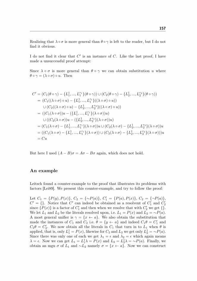
157
Realizing that λ ◦ σ is more general than θ ◦ γ is left to the reader, but I do notfind it obvious.
I do not find it clear that C ′ is an instance of C. Like the last proof, I havemade a unsuccessful proof attempt:
Since λ ◦ σ is more general than θ ◦ γ we can obtain substitution u whereθ ◦ γ = (λ ◦ σ) ◦ u. Then
C ′ = (C1(θ ◦ γ)− {L11, ..., L
r11 }(θ ◦ γ)) ∪ (C2(θ ◦ γ)− {L1
2, ..., Lr22 }(θ ◦ γ))
= (C1((λ ◦ σ) ◦ u)− {L11, ..., L
r11 }((λ ◦ σ) ◦ u))
∪ (C2((λ ◦ σ) ◦ u)− {L12, ..., L
r22 }((λ ◦ σ) ◦ u))
= ((C1(λ ◦ σ))u− ({L11, ..., L
r11 }(λ ◦ σ))u)
∪ ((C2(λ ◦ σ))u− ({L12, ..., L
r22 }(λ ◦ σ))u)
= (C1(λ ◦ σ)− {L11, ..., L
r11 }(λ ◦ σ))u ∪ (C2(λ ◦ σ)− {L1
2, ..., Lr22 }(λ ◦ σ))u
= ((C1(λ ◦ σ)− {L11, ..., L
r11 }(λ ◦ σ)) ∪ (C2(λ ◦ σ)− {L1
2, ..., Lr22 }(λ ◦ σ)))u
= Cu
But here I used (A−B)σ = Aσ −Bσ again, which does not hold.
An example
Leitsch found a counter-example to the proof that illustrates its problems withfactors [Lei89]. We present this counter-example, and try to follow the proof:
Let C1 = {P (y), P (x)}, C2 = {∼P (a)}, C ′1 = {P (a), P (x)}, C2 = {¬P (a)},C ′ = {}. Notice that C ′ can indeed be obtained as a resolvent of C ′1 and C ′2since {P (x)} is a factor of C ′1 and then when we resolve that with C ′2 we get {}.We let L1 and L2 be the literals resolved upon, i.e. L1 = P (x) and L2 = ∼P (a).A most general unifier is γ = {x ← a}. We also obtain the substitution thatmade the instances of C1 and C2 i.e. θ = {y ← a} and indeed C1θ = C ′1 andC2θ = C ′2. We now obtain all the literals in C1 that turn in to L1 when θ isapplied, that is, only L1
1 = P (x), likewise for C2 and L2 we get only L12 = ∼P (a).
Since there was only one of each we get λ1 = ε and λ2 = ε which again meansλ = ε. Now we can get L1 = L1
1λ = P (x) and L2 = L12λ = ∼P (a). Finally, we
obtain an mgu σ of L1 and ∼L2 namely σ = {x ← a}. Now we can construct
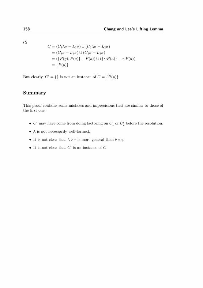
158 Chang and Lee’s Lifting Lemma
C:C = (C1λσ − L1σ) ∪ (C2λσ − L2σ)
= (C1σ − L1σ) ∪ (C2σ − L2σ)
= ({P (y), P (a)} − P (a)) ∪ ({∼P (a)} − ∼P (a))= {P (y)}
But clearly, C ′ = {} is not an instance of C = {P (y)}.
Summary
This proof contains some mistakes and imprecisions that are similar to those ofthe first one:
• C ′ may have come from doing factoring on C ′1 or C ′2 before the resolution.
• λ is not necessarily well-formed.
• It is not clear that λ ◦ σ is more general than θ ◦ γ.
• It is not clear that C ′ is an instance of C.

Bibliography
[BA12] Mordechai Ben-Ari. Mathematical Logic for Computer Science.Springer, 3rd edition, 2012.
[Ber07] Stefan Berghofer. First-order logic according to Fitting.Archive of Formal Proofs, 2007. http://afp.sf.net/entries/FOL-Fitting.shtml, Formal proof development.
[BG01] Leo Bachmair and Harald Ganzinger. Chapter 2 - resolution the-orem proving. In Alan Robinson and Andrei Voronkov, editors,Handbook of Automated Reasoning, Handbook of Automated Rea-soning, pages 19 – 99. North-Holland, Amsterdam, 2001.
[Bla15] Jasmin Christian Blanchette. Hammering away: A user’s guide toSledgehammer for Isabelle/HOL. May 2015. https://isabelle.in.tum.de/doc/sledgehammer.pdf.
[BPT14a] Jasmin Christian Blanchette, Andrei Popescu, and Dmitriy Tray-tel. Abstract completeness. Archive of Formal Proofs, April2014. http://afp.sf.net/entries/Abstract_Completeness.shtml, Formal proof development.
[BPT14b] Jasmin Christian Blanchette, Andrei Popescu, and Dmitriy Tray-tel. Unified classical logic completeness - a coinductive pearl.In Stéphane Demri, Deepak Kapur, and Christoph Weidenbach,editors, Automated Reasoning, volume 8562 of Lecture Notes inComputer Science, pages 46–60. Springer International Publish-ing, 2014.

160 BIBLIOGRAPHY
[Cha15] Amine Chaieb. The pythagorean theorem. The Isa-belle2015 Library, May 2015. https://isabelle.in.tum.de/website-Isabelle2015/dist/library/HOL/HOL-ex/Pythagoras.html.
[CL73] Chin-Liang Chang and Richard Char-Tung Lee. Symbolic Logicand Mechanical Theorem Proving. Academic Press, Inc., Orlando,FL, USA, 1st edition, 1973.
[CM00] Víctor Carreño and César Muñoz. Aircraft trajectory modelingand alerting algorithm verification. In Mark Aagaard and JohnHarrison, editors, Theorem Proving in Higher Order Logics, vol-ume 1869 of Lecture Notes in Computer Science, pages 90–105.Springer Berlin Heidelberg, 2000.
[dGRdB+15] Stijn de Gouw, Jurriaan Rot, Frank S. de Boer, Richard Bubel,and Reiner Hähnle. OpenJDK’s Java.utils.Collection.sort() isbroken: The good, the bad and the worst case. In ComputerAided Verification - 27th International Conference, CAV 2015,San Francisco, CA, USA, July 18-24, 2015, Proceedings, Part I,pages 273–289, 2015.
[EFT96] H.D. Ebbinghaus, J. Flum, and W. Thomas. Mathematical Logic.Undergraduate Texts in Mathematics. Springer New York, 1996.
[Fit96] Melvin Fitting. First-Order Logic and Automated Theorem Prov-ing. Graduate Texts in Computer Science. Springer, 1996.
[GLJ13] Jean Goubault-Larrecq and Jean-Pierre Jouannaud. The blos-som of finite semantic trees. In Andrei Voronkov and ChristophWeidenbach, editors, Programming Logics, volume 7797 of Lec-ture Notes in Computer Science, pages 90–122. Springer BerlinHeidelberg, 2013.
[Gon08] Georges Gonthier. Formal proof – the four-color theorem. Noticesof the AMS, 55(11):1382–1393, 2008.
[Har06] John Harrison. Towards self-verification of HOL Light. In Ul-rich Furbach and Natarajan Shankar, editors, Proceedings of thethird International Joint Conference, IJCAR 2006, volume 4130of Lecture Notes in Computer Science, pages 177–191, Seattle,WA, 2006. Springer-Verlag.
[Hea80] Percy John Heawood. Map-colour theorem. The quarterly journalof pure and applied mathematics, 24:332–338, 1880.
BIBLIOGRAPHY 161
[KEH+09] Gerwin Klein, Kevin Elphinstone, Gernot Heiser, June Andronick,David Cock, Philip Derrin, Dhammika Elkaduwe, Kai Engelhardt,Rafal Kolanski, Michael Norrish, Thomas Sewell, Harvey Tuch,and SimonWinwood. seL4: Formal verification of an OS kernel. InProceedings of the ACM SIGOPS 22Nd Symposium on OperatingSystems Principles, SOSP ’09, pages 207–220, New York, NY,USA, 2009. ACM.
[KNV+13] Deepak Kapur, Robert Nieuwenhuis, Andrei Voronkov, ChristophWeidenbach, and Reinhard Wilhelm. Harald Ganzinger’s legacy:Contributions to logics and programming. In Andrei Voronkovand Christoph Weidenbach, editors, Programming Logics, volume7797 of Lecture Notes in Computer Science, pages 1–18. SpringerBerlin Heidelberg, 2013.
[Lei89] Alexander Leitsch. On different concepts of resolution. Mathe-matical Logic Quarterly, 35(1):71–77, 1989.
[Lei97] Alexander Leitsch. The Resolution Calculus. Texts in theoreticalcomputer science. Springer, 1997.
[MR04] James Margetson and Tom Ridge. Completeness theorem.Archive of Formal Proofs, September 2004. http://afp.sf.net/entries/Completeness.shtml, Formal proof development.
[NK14] Tobias Nipkow and Gerwin Klein. Concrete Semantics: WithIsabelle/HOL. Springer Publishing Company, Incorporated, 2014.
[NL12] Benedikt Nordhoff and Peter Lammich. Dijkstra’s shortest pathalgorithm. Archive of Formal Proofs, January 2012. http://afp.sf.net/entries/Dijkstra_Shortest_Path.shtml, Formalproof development.
[Pau13] Lawrence C. Paulson. Gödel’s incompleteness theorems. Archiveof Formal Proofs, November 2013. http://afp.sf.net/entries/Incompleteness.shtml, Formal proof development.
[Rid04] Tom Ridge. A mechanically verified, efficient, sound and com-plete theorem prover for first order logic. Archive of For-mal Proofs, September 2004. http://afp.sf.net/entries/Verified-Prover.shtml, Formal proof development.
[Rob79] J.A. Robinson. Logic, Form and Function: The Mechanization ofDeductive Reasoning. Artificial Intelligence Series. North-Holland,1979.

162 BIBLIOGRAPHY
[RV99] Alexandre Riazanov and Andrei Voronkov. Vampire. In Au-tomated Deduction — CADE-16, volume 1632 of Lecture Notesin Computer Science, pages 292–296. Springer Berlin Heidelberg,1999.
[Sch13] Stephan Schulz. System description: E 1.8. In Logic for Program-ming, Artificial Intelligence, and Reasoning - 19th InternationalConference, LPAR-19, Stellenbosch, South Africa, December 14-19, 2013. Proceedings, pages 735–743, 2013.
[SS15] Geoff Sutcliffe and Christian Suttner. The CADE ATP systemcompetition. http://www.cs.miami.edu/~tptp/CASC/, August2015.
[Sut14] Geoff Sutcliffe. The CADE-24 Automated Theorem Proving Sys-tem Competition – CASC-24. AI Communications, 27(4):405–416,2014.
[TS09] René Thiemann and Christian Sternagel. Certification of termi-nation proofs using CeTA. In Stefan Berghofer, Tobias Nipkow,Christian Urban, and Makarius Wenzel, editors, Theorem Provingin Higher Order Logics, volume 5674 of Lecture Notes in ComputerScience, pages 452–468. Springer Berlin Heidelberg, 2009.
[WDF+09] Christoph Weidenbach, Dilyana Dimova, Arnaud Fietzke, RohitKumar, Martin Suda, and Patrick Wischnewski. SPASS version3.5. In Renate A. Schmidt, editor, Automated Deduction – CADE-22, volume 5663 of Lecture Notes in Computer Science, pages140–145. Springer Berlin Heidelberg, 2009.