A Formalization of theBerlekamp–Zassenhaus Factorization Algorithm

Jose DivasonUniversidad de La Rioja, Spain

Sebastiaan Joosten Rene ThiemannAkihisa Yamada

University of Innsbruck, Austria

AbstractWe formalize the Berlekamp–Zassenhaus algorithm for fac-toring square-free integer polynomials in Isabelle/HOL. Wefurther adapt an existing formalization of Yun’s square-freefactorization algorithm to integer polynomials, and thus pro-vide an efficient and certified factorization algorithm for ar-bitrary univariate polynomials.

The algorithm first performs a factorization in the primefield GF(p) and then performs computations in the ring ofintegers modulo pk, where both p and k are determined atruntime. Since a natural modeling of these structures via de-pendent types is not possible in Isabelle/HOL, we formalizethe whole algorithm using Isabelle’s recent addition of localtype definitions.

Through experiments we verify that our algorithm factorspolynomials of degree 100 within seconds.

Categories and Subject Descriptors F.3.1 [Logics andMeanings of Programs]: Specifying and Verifying and Rea-soning about Programs; I.1.2 [Symbolic and Algebraic Ma-nipulation]: Algorithms—Algebraic algorithms

Keywords Polynomial Factorization, Prime Fields, Isabelle

1. IntroductionModern algorithms to factor integer polynomials – follow-ing Berlekamp and Zassenhaus – work via polynomial fac-torization over prime fields GF(p) and quotient rings Z/pkZ[3, 4]. Algorithm 1 illustrates the basic structure of such analgorithm.1

1 Our algorithm starts with step 4, so that section numbers and step-numberscoincide.

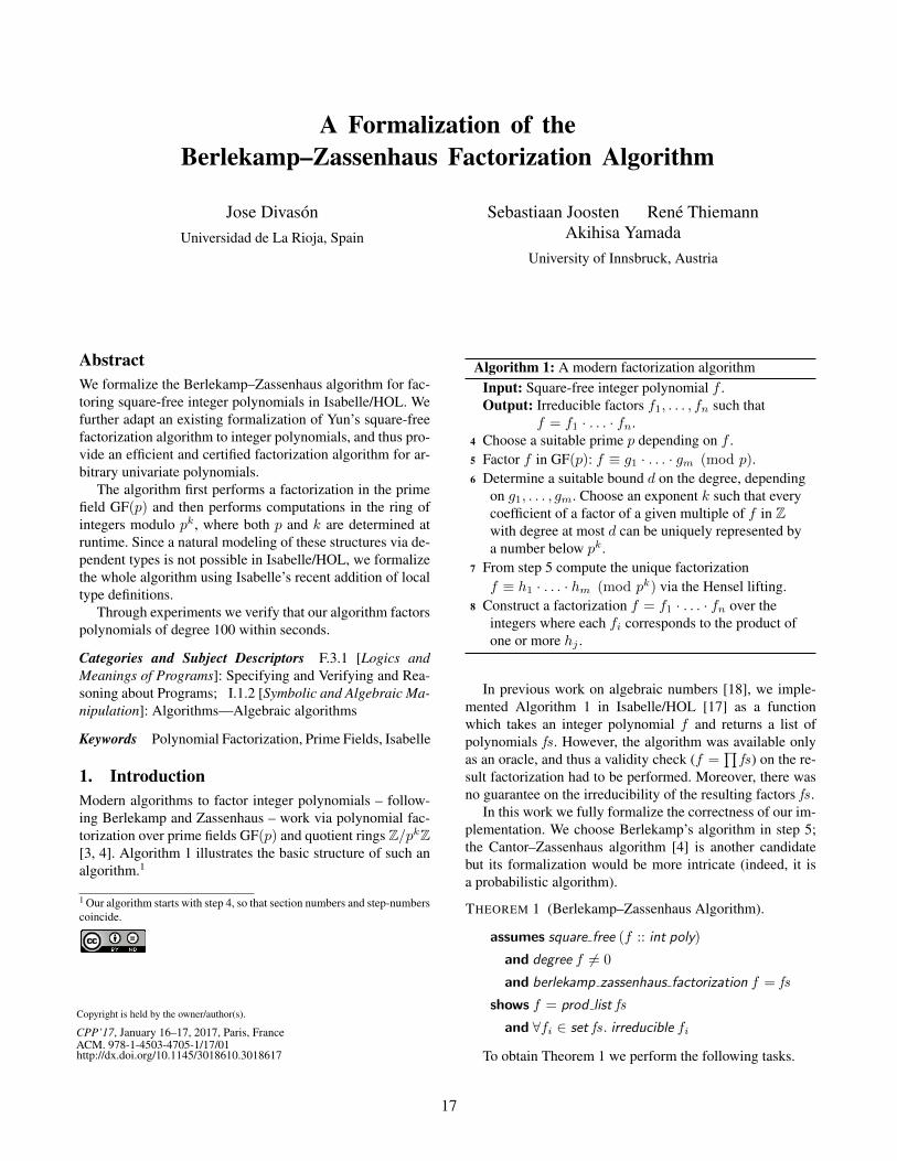
Algorithm 1: A modern factorization algorithmInput: Square-free integer polynomial f .Output: Irreducible factors f1, . . . , fn such that

f = f1 · . . . · fn.4 Choose a suitable prime p depending on f .5 Factor f in GF(p): f ≡ g1 · . . . · gm (mod p).6 Determine a suitable bound d on the degree, depending

on g1, . . . , gm. Choose an exponent k such that everycoefficient of a factor of a given multiple of f in Zwith degree at most d can be uniquely represented bya number below pk.

7 From step 5 compute the unique factorizationf ≡ h1 · . . . · hm (mod pk) via the Hensel lifting.

8 Construct a factorization f = f1 · . . . · fn over theintegers where each fi corresponds to the product ofone or more hj .

In previous work on algebraic numbers [18], we imple-mented Algorithm 1 in Isabelle/HOL [17] as a functionwhich takes an integer polynomial f and returns a list ofpolynomials fs . However, the algorithm was available onlyas an oracle, and thus a validity check (f =

∏fs) on the re-

sult factorization had to be performed. Moreover, there wasno guarantee on the irreducibility of the resulting factors fs .

In this work we fully formalize the correctness of our im-plementation. We choose Berlekamp’s algorithm in step 5;the Cantor–Zassenhaus algorithm [4] is another candidatebut its formalization would be more intricate (indeed, it isa probabilistic algorithm).

THEOREM 1 (Berlekamp–Zassenhaus Algorithm).

assumes square free (f :: int poly)

and degree f 6= 0

and berlekamp zassenhaus factorization f = fs

shows f = prod list fs

and ∀fi ∈ set fs. irreducible fi

To obtain Theorem 1 we perform the following tasks.

Copyright is held by the owner/author(s).

CPP’17, January 16–17, 2017, Paris, FranceACM. 978-1-4503-4705-1/17/01http://dx.doi.org/10.1145/3018610.3018617

17

• In Section 3 we introduce two formulations of GF(p) andZ/pkZ. We first define a type to represent these domains,employing the idea from HOL multivariate analysis thattypes can encode natural numbers by means of the car-dinality. This is essential for reusing many type-basedalgorithms from the Isabelle distribution and the AFP(Archive of Formal Proofs). At some points in our de-velopement, the type-based setting is still too restrictive.Hence we also introduce a second formulation which islocale-based [1].

• The prime p in step 4 must be chosen so that f remainssquare-free in GF(p). For the termination of the algo-rithm, we prove that such a prime always exists in Sec-tion 4.

• In Section 5, we explain Berlekamp’s algorithm, whichfactors polynomials over prime fields, and formalize itscorrectness using the type-based representation. Since Is-abelle’s code generation does not work for the type-basedrepresentation of prime fields, we define an implementa-tion of Berlekamp’s algorithm which avoids type-basedpolynomial algorithms and type-based prime fields. Thesoundness of this implementation is proved via the trans-fer package [7]: we transform the type-based sound-ness statement of Berlekamp’s algorithm into a statementwhich speaks solely about integer polynomials. Here, wecrucially rely upon local type definitions [12] to eliminatethe presence of the type for the prime field GF(p).

• For step 6 we need to find a bound on the coefficientsof the factors of a polynomial. For this purpose, we for-malize Mignotte’s factor bound in Section 6. During thisformalization task we detected a bug in our previous or-acle implementation, which computed improper boundson the degrees of factors.

• In Section 7 we formalize the Hensel lifting. As forBerlekamp’s algorithm, we first formalize basic opera-tions in the type-based setting. Unfortunately, however,this result cannot be extended to the full Hensel lifting.Therefore, we model the Hensel lifting in a locale-basedway so that modulo operation is explicitly applied onpolynomials.

• Details on step 8 are provided in Section 8 where weclosely follow the description of Knuth [9, page 452].Here, we use the same representation of polynomials overZ/pkZ as for the Hensel lifting.

• In Section 9 we adapt Yun’s square-free factorizationalgorithm [19, 21] from Q to Z. In combination with theprevious results this leads to a factorization algorithm forarbitrary integer and rational polynomials.

• Finally, we compare the efficiency of our factorizationalgorithm with the one in Mathematica 11 [20] in Sec-tion 10 and give a summary in Section 11.

To our knowledge, this is the first formalization of a mod-ern factorization algorithm. For instance, Barthe et al. reportthat there is no formalization of an efficient factorization al-gorithm over GF(p) available in Coq [2, Section 6, note 3 onformalization]. Our work is also a non-trivial case study forthe new local type definition mechanism in Isabelle.

Some key theorems leading to the algorithm have al-ready been formalized in Isabelle or other proof assistants.In ACL2, for instance, polynomials over a field are shown tobe a unique factorization domain (UFD) [5]. A more generalresult, namely that polynomials over a UFD are also a UFD,was already developed in Isabelle/HOL for implementing al-gebraic numbers [18] and an independent development byEberl is now available in the Isabelle distribution.

An Isabelle formalization of Hensel’s lemma is providedby Kobayashi et al. [10], who defined the valuations of poly-nomials via Cauchy sequences, and used this setup to provethe lemma. Consequently, their result requires a ‘valuationring’ as a precondition in their formalization. While this ex-tra precondition is theoretically met in our setting, we did notattempt to reuse their results, because the type of polynomi-als in their formalization (from HOL-Algebra) differs fromthe polynomials in our development (from HOL/Library).Instead, we formalize a direct proof for Hensel’s lemma.Our formalizations are incomparable: On the one hand,Kobayashi et al. did not restrict to integer polynomials aswe do. On the other hand, we additionally formalize thequadratic Hensel lifting [22], extend the lifting from binaryto n-ary factorizations, and prove a uniqueness result, whichis required for proving Theorem 1.

A Coq formalization of Hensel’s lemma is also available.It is used for certifying integral roots and ‘hardest-to-roundcomputation’ [14]. If one is interested in certifying a fac-torization, rather than a certified algorithm that performs it,it suffices to test that all the found factors are irreducible.Kirkels [8] formalized a sufficient criterion for this test inCoq: when a polynomial is irreducible modulo some prime,it is also irreducible in Z. Both formalizations are in Coq,and we did not attempt to reuse them.

Our formalization is available in the AFP and details onthe experiments are provided at

http://cl-informatik.uibk.ac.at/software/

ceta/experiments/factorization.

The formalization as described in this paper corresponds toAFP revision c57b0e9b0d65, which compiles with Isabellerevision 03057a8fdd1f.

2. PreliminariesOur formalization is based on Isabelle/HOL, and we statetheorems, as well as certain definitions, following Isabelle’ssyntax. For instance, f :: α ⇒ α poly indicates that f isa function that maps α to a polynomial over α. Isabelle’skeywords are written in bold. Other symbols are either clear

18

from their notation, or defined on their appearance. We onlyassume the HOL axioms and local type definitions, andensure that Isabelle can build our theories. Consequently, asceptical reader that trusts the soundness of Isabelle/HOLonly needs to check the definitions, as the proofs are checkedby Isabelle.

We expect the reader to be familiar with algebra, and usesome of its standard notions without further explanation.Concerning notation, we write f ′ for the derivative of apolynomial f , lc(f) for the leading coefficient of f , andres(f, g) for the resultant of f and another polynomial g.

A factorization of a polynomial f is a decompositioninto irreducible factors f1, . . . , fn such that f = f1 · . . . ·fn. Whereas the irreducibility of a ring element x is oftendefined via divisibility (denoted by the binary relation dvdfollowing Isabelle):

¬x dvd 1 ∧(∀y. y dvd x −→ y dvd 1 ∨ x dvd y

)(1)

in this paper we define irreducibility of a polynomial f as

degree f 6= 0 ∧(∀g. g dvd f −→ degree g ∈ {0, degree f}

). (2)

Note that (1) and (2) are not equivalent on integer polyno-mials; e.g., a factorization of f = 10x2 − 10 in terms of (1)will be f = 2·5·(x−1)·(x+1), where the prime factorizationof the content, i.e., the GCD of the coefficients, has to be per-formed. In contrast, (2) does not demand a prime factoriza-tion, and a factorization may be f = (10x−10) ·(x+1). Al-gorithm 1 will produce the latter factorization, where all fac-tors except for one are content-free, i.e., whose content is 1.Note that definitions (1) and (2) are equivalent on content-free polynomials (and in particular for field polynomials).

In a similar way to irreducibility, we also define that apolynomial f is square-free if there does not exist a non-constant polynomial g such that g2 divides f . In particular,the integer polynomial 22x is square-free.

3. Formalizing Prime FieldsHere we introduce two formalizations of the quotient ringZ/pkZ and the prime field GF(p): a type-based version andlocale-based version.

3.1 Type-Based FormalizationWe first define a polymorphic type to represent Z/pZ foran arbitrary p > 0, which forms the prime field GF(p)when p is a prime. The advantage of having GF(p) availableas a type is that we can reuse several algorithms that areavailable only in type-based settings, e.g., the Gauss–Jordanelimination, GCD computation for polynomials, square-freefactorization, etc.

Since Isabelle does not support dependent types, we can-not directly use the term variable p in a type definition. To

overcome the problem, we reuse the idea of the vector repre-sentation from HOL multivariate analysis: types can encodenatural numbers. We encode p as CARD(α), i.e., the cardi-nality of the universe of a (finite) type represented by a typevariable α.

typedef (α :: finite) mod ring = {0 ..< CARD(α)}

Given a finite type α with p elements, α mod ring is atype with elements 0, . . . , p − 1. With the help of the lift-ing and transfer package, we naturally define arithmetic inα mod ring modulo CARD(α); for instance, multiplicationis defined as follows:

lift definition times mod ring ::

α mod ring ⇒ α mod ring ⇒ α mod ring

is λx y. (x ∗ y) mod CARD(α)

It is straightforward to show that α mod ring forms a com-mutative ring:

instantiation mod ring :: (finite) comm ring

Note that comm ring does not assume the existence of themultiplicative unit 1 . If CARD(α) = 1, then α mod ring isnot an instance of the type class ring 1 , for which 0 6= 1 isrequired. Hence we introduce the following type class:

class nontriv = assumes CARD(α) > 1

and derive the following instantiation:2

instantiation mod ring :: (nontriv) comm ring 1

It is well known that the ring of integers modulo someprime number forms a field. To enforce that the modulus isa prime number, we employ the same trick as above.

class prime card = assumes prime (CARD(α))

The key to being a field is the existence of the multiplica-tive inverse x−1. This follows from Fermat’s little theorem:

x · xp−2 ≡ xp−1 ≡ 1 (mod p)

for any nonzero integer x and prime p; that is, x−1 =xCARD(α)−2 if CARD(α) is a prime. The theorem is alreadyavailable in the Isabelle distribution for the integers, andwe just have to apply the transfer tactic to lift the result to(α :: prime card) mod ring.

instantiation mod ring :: (prime card) field

In the rest of the paper, we write α GFp instead of (α ::prime card) mod ring.3

2 A formalization of the ring Z/pZ is already present in ~~/src/HOL/

Library/Numeral_Type as a locale mod ring . In principle we couldreuse results from the library by proving connection between the locale andour class; however, as the resulting proofs became slightly longer than directproofs, we did not use this library.3 We would like to have introduced this abbreviation also in Isabelle. How-ever, we are not aware of how to do this, since the type synonym keyworddoes not allow specifying type constraints such as α :: prime card.

19

For efficiency, we compute xp−2 using the binary ex-ponentiation algorithm. Another approach for computingx−1 would use the extended Euclidean algorithm; however,through experiments we observed that this approach is ben-eficial only when p is quite large (such as 20 digits). Since inour application p is usually small, we compute x−1 as xp−2.

3.2 Locale-Based VersionThe type-based setting is preferable whenever possible,since it allows concise theorem statements and better sup-port for proof automation, cf. Kuncar and Popescu [12].

At some points of our development, however, the type-based approach is not expressive enough; cf. Section 7. Wemust reason about the ring of integers modulo m, where mcannot be given via type variables.

Hence, we also introduce a locale poly mod whichfixes the modulus m and defines modular arithmetic oper-ations on type int poly . In particular, Mpm :: int poly ⇒int poly is a function that pointwise takes modulo m ofeach coefficients. Other operations, such as equivalence≡m,coprimem, unique factorizationm, are defined with the helpof Mp; e.g., f ≡m g is defined as Mpm f = Mpm g.

4. Square-Free Polynomials in GF(p)In Algorithm 1, step 4 mentions the selection of a suitableprime p. To be more precise, there are two conditions thathave to be satisfied. First, p must be coprime to the lead-ing coefficient of the input polynomial f . The other condi-tion stems from Berlekamp’s algorithm, namely f must besquare-free in GF(p).

Whereas selecting a prime that satisfies the first conditionis in principle easy – any prime larger than the leadingcoefficient will do – it is actually not so easy to formallyprove that the second condition is satisfiable. We split theproblem of computing a suitable prime into the followingsteps.

• Prove that if f is square-free, then f and its derivative f ′

are coprime in GF(p), and f is square-free in GF(p) forevery sufficiently large prime p.

• Develop a prime number generator which returns the firstprime such that f and f ′ are coprime in GF(p).

The prime number generator lazily generates all primesand aborts as soon as the first suitable prime is detected.This is easy to model in Isabelle by defining the generator(suitable prime bz) via partial function [11].

Our formalized proof of the existence of a suitable primeproceeds along the following line. Let f be square-free overZ. Then f is also square-free over Q using Gauss Lemma.For fields of characteristic 0, f is square-free if and only iff and f ′ are coprime. Coprimality is the same as demandingthat the resultant is non-zero, so we get res(f, f ′) 6= 0.The advantage of using resultants is that they admit thefollowing property: if p is larger than res(f, f ′) and the

leading coefficients of f and f ′, then resp(f, f′) 6= 0, where

resp(f, g) denotes the resultant of f and g computed inGF(p). Now we go back from resultants to coprimality, andobtain that f and f ′ are coprime in GF(p). Finally we provethat the coprimality of f and f ′ ensures square-freeness inarbitrary fields.

Whereas the reasoning above shows that any prime largerthan res(f, f ′), lc(f) and lc(f ′) is admitted, we still preferto search for a small prime p since Berlekamp’s algorithmhas a worst case lower bound of degree(f) · p operations.

EXAMPLE 1. Consider the polynomial f which will be usedas a running example throughout this paper.

f = 4 + 47x− 2x2 − 23x3 + 18x4 + 10x5

Selecting p = 2 or p = 5 is not admissible since thesenumbers are not coprime to 10, the leading coefficient of f .Also p = 3 is not admissible since the GCD of f and f ′ is2 + x in GF(3). Finally, p = 7 is a valid choice since theGCD of f and f ′ is 1 in GF(7), and 7 and 10 are coprime.

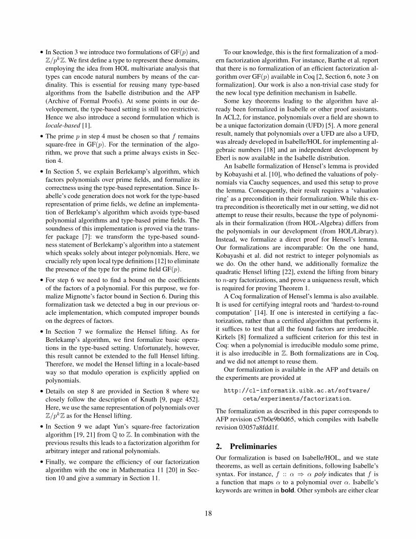
5. Berlekamp’s Algorithm5.1 Informal DescriptionAlgorithm 2 briefly describes Berlekamp’s algorithm [3]. Itfocuses on the core computations that have to be performed.For a discussion on why these steps are performed we referto Knuth [9, Section 4.6.2].

Algorithm 2: Berlekamp’s factorization algorithmInput: Square-free polynomial f over GF(p) of degree

d 6= 0.Output: Constant c and set F of monic and irreducible

factors f1, . . . , fn such that f = c · f1 · . . . · fn1 Let c be the leading coefficient of f . Update f := f/c.2 Compute the Berlekamp matrix Bf ∈ GF(p)d×d for f ,

where the i-th row is the vector of the coefficients ofpolynomial xp·i mod f .

3 Compute the dimension r and a basis b1, . . . , br of theleft null space of Bf − I , where I is the identitymatrix of size d× d.

4 For each basis vector bi construct the correspondingpolynomial hi where the entries in bi are thecoefficients of hi.

5 Set F := {f}, H := {h1, . . . , hr} \ {1}, FI := ∅.6 If |F | = r ∨H = ∅, return c and F ∪ FI .7 Pick h ∈ H and update H := H \ {h}.

Update F := {gij | fi ∈ F, 0 ≤ j < p, gij =gcd(fi, h− j), gij 6= 1}.

8 If one can find k irreducible polynomials in F , movethem to FI and update r := r − k.

9 Goto step 6.

We illustrate the algorithm by continuing Example 1.

20

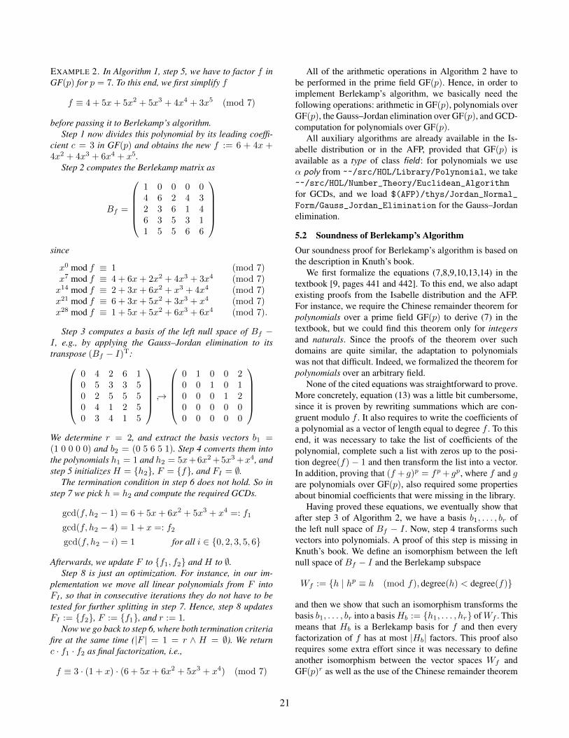
EXAMPLE 2. In Algorithm 1, step 5, we have to factor f inGF(p) for p = 7. To this end, we first simplify f

f ≡ 4 + 5x+ 5x2 + 5x3 + 4x4 + 3x5 (mod 7)

before passing it to Berlekamp’s algorithm.Step 1 now divides this polynomial by its leading coeffi-

cient c = 3 in GF(p) and obtains the new f := 6 + 4x +4x2 + 4x3 + 6x4 + x5.

Step 2 computes the Berlekamp matrix as

Bf =

1 0 0 0 04 6 2 4 32 3 6 1 46 3 5 3 11 5 5 6 6

since

x0 mod f ≡ 1 (mod 7)x7 mod f ≡ 4 + 6x+ 2x2 + 4x3 + 3x4 (mod 7)x14 mod f ≡ 2 + 3x+ 6x2 + x3 + 4x4 (mod 7)x21 mod f ≡ 6 + 3x+ 5x2 + 3x3 + x4 (mod 7)x28 mod f ≡ 1 + 5x+ 5x2 + 6x3 + 6x4 (mod 7).

Step 3 computes a basis of the left null space of Bf −I , e.g., by applying the Gauss–Jordan elimination to itstranspose (Bf − I)T:

0 4 2 6 10 5 3 3 50 2 5 5 50 4 1 2 50 3 4 1 5

↪→

0 1 0 0 20 0 1 0 10 0 0 1 20 0 0 0 00 0 0 0 0

We determine r = 2, and extract the basis vectors b1 =(1 0 0 0 0) and b2 = (0 5 6 5 1). Step 4 converts them intothe polynomials h1 = 1 and h2 = 5x+6x2+5x3+x4, andstep 5 initializes H = {h2}, F = {f}, and FI = ∅.

The termination condition in step 6 does not hold. So instep 7 we pick h = h2 and compute the required GCDs.

gcd(f, h2 − 1) = 6 + 5x+ 6x2 + 5x3 + x4 =: f1

gcd(f, h2 − 4) = 1 + x =: f2

gcd(f, h2 − i) = 1 for all i ∈ {0, 2, 3, 5, 6}

Afterwards, we update F to {f1, f2} and H to ∅.Step 8 is just an optimization. For instance, in our im-

plementation we move all linear polynomials from F intoFI , so that in consecutive iterations they do not have to betested for further splitting in step 7. Hence, step 8 updatesFI := {f2}, F := {f1}, and r := 1.

Now we go back to step 6, where both termination criteriafire at the same time (|F | = 1 = r ∧ H = ∅). We returnc · f1 · f2 as final factorization, i.e.,

f ≡ 3 · (1 + x) · (6 + 5x+ 6x2 + 5x3 + x4) (mod 7)

All of the arithmetic operations in Algorithm 2 have tobe performed in the prime field GF(p). Hence, in order toimplement Berlekamp’s algorithm, we basically need thefollowing operations: arithmetic in GF(p), polynomials overGF(p), the Gauss–Jordan elimination over GF(p), and GCD-computation for polynomials over GF(p).

All auxiliary algorithms are already available in the Is-abelle distribution or in the AFP, provided that GF(p) isavailable as a type of class field : for polynomials we useα poly from ~~/src/HOL/Library/Polynomial, we take~~/src/HOL/Number_Theory/Euclidean_Algorithm

for GCDs, and we load $(AFP)/thys/Jordan_Normal_

Form/Gauss_Jordan_Elimination for the Gauss–Jordanelimination.

5.2 Soundness of Berlekamp’s AlgorithmOur soundness proof for Berlekamp’s algorithm is based onthe description in Knuth’s book.

We first formalize the equations (7,8,9,10,13,14) in thetextbook [9, pages 441 and 442]. To this end, we also adaptexisting proofs from the Isabelle distribution and the AFP.For instance, we require the Chinese remainder theorem forpolynomials over a prime field GF(p) to derive (7) in thetextbook, but we could find this theorem only for integersand naturals. Since the proofs of the theorem over suchdomains are quite similar, the adaptation to polynomialswas not that difficult. Indeed, we formalized the theorem forpolynomials over an arbitrary field.

None of the cited equations was straightforward to prove.More concretely, equation (13) was a little bit cumbersome,since it is proven by rewriting summations which are con-gruent modulo f . It also requires to write the coefficients ofa polynomial as a vector of length equal to degree f . To thisend, it was necessary to take the list of coefficients of thepolynomial, complete such a list with zeros up to the posi-tion degree(f) − 1 and then transform the list into a vector.In addition, proving that (f + g)p = fp+ gp, where f and gare polynomials over GF(p), also required some propertiesabout binomial coefficients that were missing in the library.

Having proved these equations, we eventually show thatafter step 3 of Algorithm 2, we have a basis b1, . . . , br ofthe left null space of Bf − I . Now, step 4 transforms suchvectors into polynomials. A proof of this step is missing inKnuth’s book. We define an isomorphism between the leftnull space of Bf − I and the Berlekamp subspace

Wf := {h | hp ≡ h (mod f), degree(h) < degree(f)}

and then we show that such an isomorphism transforms thebasis b1, . . . , br into a basisHb := {h1, . . . , hr} ofWf . Thismeans that Hb is a Berlekamp basis for f and then everyfactorization of f has at most |Hb| factors. This proof alsorequires some extra effort since it was necessary to defineanother isomorphism between the vector spaces Wf andGF(p)r as well as the use of the Chinese remainder theorem

21

over polynomials and the uniqueness of the solution. Inorder to carry out these proofs, we also extend an existingAFP entry by Lee [13] about vector spaces to include somenecessary results which relate linear maps, isomorphismsbetween vector spaces, dimensions, and bases.

Once having proved that Hb is a Berlekamp basis for f ,we can prove equality (14); for every divisor fi of f andevery h ∈ Hb, we have

fi =∏

0≤j<p

gcd(fi, h− j). (14)

Finally, it follows that every non-constant reducible divi-sor fi of f can be properly factored via gcd(fi, h − j) forsuitable h ∈ Hb and 0 ≤ j < p.

In order to prove the soundness of steps 5–9 in Algo-rithm 2, we use the following invariants – these are not soexplicitly stated by Knuth as the equations. Here, Hold rep-resents the set of already processed polynomials of Hb.

1. f =∏(F ∪ FI).

2. All fi ∈ F ∪ FI are monic and non-constant.

3. All fi ∈ FI are irreducible.

4. Hb = H ∪Hold.

5. gcd(fi, h− j) ∈ {1, fi} for all h ∈ Hold, 0 ≤ j < p andfi ∈ F ∪ FI .

6. |FI |+ r = |Hb|.It is easy to see that all invariants are initially established

in step 5 by picking Hold = {1} ∩Hb. In particular, invari-ant 5 is satisfied since the GCD of the monic polynomial fand a constant polynomial c is always 1 (if c 6= 0) or f (ifc = 0).

It is also not hard to see that step 7 preserves the invari-ants. In particular, invariant 5 is satisfied for elements in FIsince these are irreducible. Invariant 1 follows from (14).

The irreducibility of the final factors that are returnedin step 6 can be argued as follows. If |F | = r, then byinvariant 6 we know that |Hb| = |F ∪ FI |, i.e., F ∪ FIis a factorization of f with the maximum number of factors,and thus every factor is irreducible. In the other case, H = ∅and hence Hold = Hb by invariant 4. Combining this withinvariant 5 shows that every element fi in F ∪ FI cannot befactored by gcd(fi, h − j) for any h ∈ Hb and 0 ≤ j < p.Since Hb is a Berlekamp basis, this means that fi must beirreducible.

Eventually, putting everything together we arrive at theformalized main soundness statement of Berlekamp’s al-gorithm. Here, mset converts a list into a multiset, andunique factorization f demands that the given factorizationis the unique factorization of f .

THEOREM 2 (Berlekamp’s Algorithm).

assumes square free (f :: α GFp poly)

and berlekamp factorization f = (c, fs)

shows unique factorization f (c,mset fs)

In order to prove the validity of the output factorization,we basically use the invariants mentioned before. However,it still requires some tedious reasoning.

Uniqueness follows from the general theorem that thepolynomials over fields form a unique factorization domain.

In the proofs, most of the time we model products ofpolynomials (

∏fs) via prod list (the product of the elements

of a list) instead of using prod (the product of the elementsof a set). The reason is that prod list has nicer properties.For instance prod list (f#fs) = f · prod list fs alwaysholds (here # is the Isabelle’s syntax for the list constructor),whereas prod (insert f F ) = f · prod F is ensured only iff /∈ F and F is a finite set. An alternative to prod list mightbe products over multisets. However this will require manyconversions from lists to multisets since our algorithms workon lists.

5.3 Implementing Berlekamp’s AlgorithmThe soundness of Theorem 2 is formulated in a type-basedsetting. In particular, the function berlekamp factorizationhas type

α GFp poly⇒ αGFp× αGFp poly list.

In our use case, recall that Algorithm 1 first computes aprime number p, and then invokes Berlekamp’s algorithm onGF(p). This requires Algorithm 1 to construct a new type Pwith CARD(P ) = p depending on the value of p, and theninvoke berlekamp factorization for type P GFp.

Unfortunately, this is not possible in Isabelle/HOL. Hence,Algorithm 1 requires Berlekamp’s algorithm to have a typelike

int⇒ int poly⇒ int× int poly list

where the first argument is the dynamically chosen prime p.As a first step to solve this problem we define conver-

sions to int :: αGFp ⇒ int and of int :: int ⇒ αGFpbetween αGFp and int where the former is injective, andthe other one applies one “modulo CARD(α)” operation.These conversions are then lifted homomorphically to poly-nomials, resulting in functions to int poly and of int poly.With the help of these conversions and some homomorphismlemmas we formulate and prove the following statementof Berlekamp’s algorithm, which speaks about propertiesof integer polynomials f and integer factors fs . Now onlythe invocation of Berlekamp’s algorithm requires αGFp. Inthe lemma, unique factorizationp and square freep denote aunique factorization and a square-free polynomial modulo prespectively.

LEMMA 1.

assumes (g :: α GFp) = of int poly f

and square freep f

and berlekamp factorization g = (d, gs)

22

and c = to int d

and fs = map to int poly gs

and p = CARD(α)

shows unique factorizationp f (c,mset fs)

The next step consists of implementing Berlekamp’s al-gorithm on integer polynomials (mod p) directly. This imple-mentation cannot use the polynomial and matrix algorithmsdirectly as these are type-based, cf. Section 3.

Instead, we made copies of the algorithms, but instead ofusing the type-based arithmetic operations, we use a recordops as parameter that stores all the required arithmetic oper-ations plus , mult, etc. To be more precise, whenever someauxiliary algorithm A invokes x + y in the type-based ver-sion, we replace it by x+′ops y, denoting plus ops x y (plus isthe record selector), and pass ops as an additional argumentto A′, the record-based version of A.

The soundness of the record-based algorithms is thenmainly proved with the help of the transfer package. We de-fine relations which express that certain elements are rep-resentatives of each other. For instance, for integers andGF(p) we define GFprel :: int ⇒ αGFp ⇒ bool asGFprel x y = (x = to int y). Similar relations are then con-structed for polynomials and matrices, e.g., polyrel R xs f =(list all2 R xs (coeffs f)) relates lists with polynomials,where list all2 R xs ys demands that xs and ys are of equallengths and their elements are point-wise in relation R.

Then we define a locale demanding that ops faithfullyimplements the arithmetic operations in GF(p), expressedas a set of transfer rules (cf. [7]) of the following form.

(GFprel ===> GFprel ===> GFprel) (op +′ops) (op +)

(GFprel ===> GFprel) inverse′ops inverse

(GFprel ===> GFprel ===> op =) (op =) (op =)

For instance, the first rule states that if the arguments x and yare related to arguments x and y, resp., then x+y is related tox+′ops y. Note that equality is not part of the record ops. Thisbecomes visible in the last transfer rule which expresses thatequality on GF(p) can be implemented as equality on therepresenting integers.

Within the locale, we finally prove the soundness of theimplementation for Berlekamp’s algorithm.

THEOREM 3 (Implementation of Berlekamp).

(polyrel GFprel ===> GFprel ×rel list all2 (polyrel GFprel))

(berlekamp factorization′ops) berlekamp factorization

The theorem states that if the input f represents some GF(p)polynomial g, and berlekamp factorization′ ops f = (c, fs)and berlekamp factorization g = (d, gs), then c representsd and fs represents gs .

To obtain Theorem 3 we developed transfer rules for allauxiliary algorithms that are invoked in Berlekamp’s algo-rithm. Here, the diagnostic commands transfer prover start

and transfer step were helpful to see why certain transferrules could initially not be proved automatically; these com-mands nicely pointed to missing transfer rules.

Most of the transfer rules for non-recursive algorithmswere proved mainly by unfolding the definitions and finish-ing the proof by transfer prover. For recursive algorithms,we often perform induction via the algorithm. To handle aninductive case, we locally declare transfer rules (obtainedfrom the induction hypothesis), unfold one function applica-tion iteration, and then finish the proof by transfer prover.

Still, problems arose in case of underspecification. Forinstance it is impossible to prove an unconditional transferrule for the function hd that returns the head of a list usingthe standard relator for lists, (list all2 R ===> R) hd hd;when the lists are empty, we have to relate undefined :: αwith undefined :: β. To circumvent this problem, we hadto reprove invariants that hd is invoked only on non-emptylists.

Similar problems arose when using matrix indices wheretransfer rules between matrix entries Aij and Bij are avail-able only if i and j are within the matrix dimensions. So,again we had to reprove the invariants on valid indices – justunfolding the definition and invoking transfer prover wasnot sufficient.

In summary, the development of the separate implemen-tation is some annoying overhead, but still a workable so-lution. In numbers: Theorem 2 requires around 3000 linesof difficult proofs whereas Theorem 3 demands around 600lines of easy proofs.

Using Theorem 3 we can now reformulate the sound-ness of Berlekamp’s algorithm (Lemma 1) as follows. Here,ff ops p is the record that implements arithmetic in GF(p) asrequired by the locale, and poly of list converts a coefficientlist into a polynomial.

LEMMA 2.

assumes g = coeffs (Mpp f)

and square freep f

and berlekamp factorization′ (ff ops p) g = (c, gs)

and fs = map poly of list gs

and p = CARD(α :: prime card)

shows unique factorizationp f (c,mset fs)

Note that in Lemma 2 the occurrence of the type αGFpvanished. All constants and types involved speak about in-tegers, integer polynomials, and integer lists, except for thesingle occurrence of CARD(α :: prime card).

Finally, we delete this last occurrence of α with the helpof local type definitions, a recent addition to the Isabelledistribution. It replaces the condition p = CARD(α ::prime card) by prime p. Thus we can define a functionberlekamp factorization int :: int ⇒ int poly ⇒ int ×int poly list and prove its soundness without having to createa type αGFp.

23

THEOREM 4 (Berlekamp Factorization on Integers).

assumes berlekamp factorization int p f = (c, fs)

and square freep f

and prime p

shows unique factorizationp f (c,mset fs)

6. Mignotte’s Factor BoundReconstructing the polynomials proceeds by obtaining fac-tors modulo pk. The value of k should be large enough, sothat any coefficient of any factor of the original polynomialcan be determined from the corresponding coefficients inZ/pkZ. We can find such k by finding a bound on the co-efficients of the factors of f , i.e., a function factor boundsuch that the following statement holds:

assumes f 6= 0

and g · h = f

and degree(g) ≤ dshows |coeff g j| ≤ factor bound f d

Clearly, if b is a bound on the absolute value of thecoefficients, and pk > 2 · b then we can encode all re-quired coefficients: In Z/pkZ we can represent the numbers{−bp

k−12 c, . . . , d

pk−12 e} ⊇ {−b, . . . , b}.

The Mignotte bound [15] provides a bound on the abso-lute values of the coefficients. The Mignotte bound is ob-tained by relating the Mahler measure of a polynomial to itscoefficients. The Mahler measure is defined as follows:

measure f = |lc(f)| ·n∏i=1

max{1, |ri|}

where n = degree(f) and r1, . . . , rn are the complex rootsof f taking multiplicity into account. For nonzero f , lc(f) isa nonzero integer. It follows that measure f ≥ 1. The defi-nition of measure shows that measure (g · h) = measure g ·measure h. We conclude that measure g ≤ measure f if g isa factor of f .

The Mahler measure is bounded by the coefficients fromabove through Landau’s inequality:

measure f ≤√∑n

i=1 (coeff f i)2

Mignotte showed that the coefficients also bound themeasure from below: |coeff g i| ≤

(di

)·measure g whenever

degree(g) ≤ d. Putting this together we get:

|coeff g j| ≤(d

j

)·measure g

≤(

d

bd/2c

)·measure f

≤(

d

bd/2c

)·√∑

i (coeff f i)2

=

√(d

bd/2c

)2

·∑i (coeff f i)2

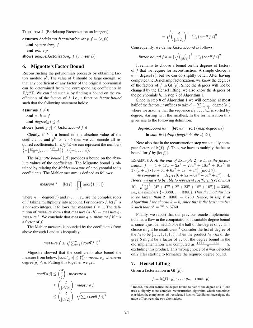
Consequently, we define factor bound as follows:

factor bound f d = b√(

dbd/2c

)2 ·∑i (coeff f i)2c

It remains to choose a bound on the degrees of factorsof f that we require for reconstruction. A simple choice isd = degree(f), but we can do slightly better. After havingcomputed the Berlekamp factorization, we know the degreesof the factors of f in GF(p). Since the degrees will not bechanged by the Hensel lifting, we also know the degrees ofthe polynomials hi in step 7 of Algorithm 1.

Since in step 8 of Algorithm 1 we will combine at mosthalf of the factors, it suffices to take d =

∑mi=bm2 c

degree(hi),where we assume that the sequence h1, . . . , hm is sorted bydegree, starting with the smallest. In the formalization thisgives rise to the following definition:

degree bound hs = (let ds = sort (map degree hs)

in sum list (drop (length ds div 2) ds))

Note also that in the reconstruction step we actually com-pute factors of lc(f) ·f . Thus, we have to multiply the factorbound for f by |lc(f)|.

EXAMPLE 3. At the end of Example 2 we have the factor-ization f = 4 + 47x − 2x2 − 23x3 + 18x4 + 10x5 ≡3 · (1 + x) · (6 + 5x+ 6x2 + 5x3 + x4) (mod 7).

We compute d = degree(6 + 5x+ 6x2 + 5x3 + x4) = 4.Hence, we have to be able to represent coefficients of at most

10 ·b√(

42

)2 · (42 + 472 + 22 + 232 + 182 + 102)c = 3380,i.e., the numbers {−3380, . . . , 3380}. Thus the modulus hasto be larger than 2 · 3380 = 6760. Hence, in step 6 ofAlgorithm 1 we choose k = 5, since this is the least numberk such that pk = 7k > 6760.

Finally, we report that our previous oracle implementa-tion had a flaw in the computation of a suitable degree boundd, since it just defined d to be the half of the degree of f . Thischoice might be insufficient:4 Consider the list of degree ofthe hi to be [1, 1, 1, 1, 1, 5]. Then the product h1 · h6 of de-gree 6 might be a factor of f , but the degree bound in theold implementation was computed as 1+1+1+1+1+5

2 = 5,excluding this product. This wrong choice of d was detectedonly after starting to formalize the required degree bound.

7. Hensel LiftingGiven a factorization in GF(p):

f ≡ lc(f) · g1 · . . . · gm (mod p)

4 Indeed, one can reduce the degree bound to half of the degree of f if oneuses a slightly more complex reconstruction algorithm which sometimesconsiders the complement of the selected factors. We did not investigate thetrade-off between the two alternatives.

24

which Berlekamp’s algorithm provides, the task of theHensel lifting is to compute a factorization

f ≡ lc(f) · h1 · . . . · hm (mod pk).

Hensel’s lemma, following Miola and Yun [16], is stated asfollows.

LEMMA 3 (Hensel). Consider polynomials f over Z, g1and h1 over GF(p) for a prime p, such that g1 is monic andf ≡ g1 ·h1 (mod p). For any k ≥ 1, there exist polynomialsgk and hk over Z/pkZ such that gk is monic, f ≡ gk · hk(mod pk), gk ≡ g1 (mod p), hk ≡ h1 (mod p). Moreover,if f is monic, then gk and hk are unique (mod pk).

The lemma is proved inductively on k where there is a onestep lifting from Z/pkZ to Z/pk+1Z. To be more precise, theone step lifting assumes polynomials gk and hk over Z/pkZsatisfying the conditions, and computes the desired gk+1 andhk+1 over Z/pk+1Z.

As explained in Section 3, it is preferable to carry onthe proof in the type-based setting whenever possible, andindeed we proved the one step lifting in this way.

LEMMA 4 (Hensel lifting – one step).

assumes CARD(α) = CARD(β :: prime card) ∗ CARD(γ)

and CARD(β) dvd CARD(γ)

and #f = g ∗ hand monic g

and degree f = degree g + degree h

and hensel 1 TYPE(β) f g h = (g, h)

shows f = g ∗ h ∧ monic g ∧ g = #g ∧ h = #h ∧degree g = degree g ∧ degree h = degree h

and . . . (* uniqueness statement *)

Here, CARD(α) represents pk+1, CARD(β) represents p,and CARD(γ) represents pk. The prefix “#” denotes thefunction that converts polynomials over integer modulo minto those over integer modulo n, where the type inferencedetermines n.

Unfortunately, we could not see how to use Lemma 4 inthe inductive proof of Lemma 3 in a type-based setting. Atype-based statement of Lemma 3 would have an assumptionlike CARD(α) = pk. Then the induction hypothesis wouldlook like

CARD(α) = pk =⇒ . . . (3)

and the goal statement would be CARD(α) = pk+1 =⇒ . . . .There is no hope to be able to apply the induction hypothesis(3) for this goal, since the assumptions are clearly incompat-ible. A solution to this problem seems to require extendingthe induction scheme to admit changing the type variables,and produce an induction hypothesis like CARD(?α) =pk =⇒ . . . where ?α can be instantiated. Unfortunately thisis not possible in Isabelle/HOL.

In our development, we therefore formalized most of thereasoning for Hensel’s lemma on integer polynomials in thelocale-based setting (cf. Section 3.2), so that the modulus(the k in the pk) can be easily altered within algorithmsand inductive proofs. Working on integer polynomials alsohas the advantage when formalizing both the Hensel lift-ing, which is presented below, and the reconstruction phase,which is presented in the next section, since one has to per-form operations of integer polynomials both in Z and inZ/pkZ, so there is no conversion required.

In the locale poly mod , the binary version of Hensel’slemma is proved as follows, and internally one step of theHensel lifting is applied over and over again, i.e., the expo-nents are p, p2, p3, p4, . . . [16, Sect. 2.2]. In the statement,Isabelle’s syntax ∃! represents the unique existential quan-tification.

LEMMA 5 (Hensel lifting – multiple steps, binary).

assumes prime p and coprimep g h and f ≡p g · hand Mpp g = g and Mpp h = h

and monic g and k 6= 0

shows ∃! (g, h). f ≡pk g · h ∧monic g ∧ g ≡p g ∧ h ≡p h ∧Mppk g = g ∧Mppk h = h

We also formalize the quadratic Hensel lifting, where themodulus during the lifting will be p, p2, p4, p8, . . . , p2

`

where, ` is a suitable exponent such that 2` ≥ k, cf. [16,Sect. 2.3]. Since 2` might be larger than k, we finally per-form a Mppk -operation in order to convert the Z/p2`Z fac-torization into a Z/pkZ factorization. The quadratic versionis supported in addition to the linear version, since in our ex-periments the quadratic algorithm is more efficient than thelinear one in contrast to the result of Miola and Yun [16, Sect.1].56 Hence, the soundness lemma for the quadratic Hensellifting does not only mention the existence of f and g, but itproves that the algorithm computes these polynomials.

We further extend the binary (quadratic) lifting algorithmto an executable n-ary lifting algorithm: hensel lifting.

LEMMA 6 (Hensel Lifting – general case).

assumes hensel lifting p k f fs = gs

and k 6= 0 and prime p and coprime (lc(f)) p

and square freep f and factorizationp f (c,mset fs)

and c ∈ {0.. < p}and ∀fi ∈ set fs. set (coeffs fi) ⊆ {0.. < p}

shows unique factorizationpk f (lc(f),mset gs)

and ∀gi ∈ set gs. monic gi ∧ irreduciblep gi

5 Perhaps our quadratic version of Hensel lifting is faster than the linearversion since we did not integrate (and prove) optimization (iv) of Miolaand Yun [16, Sect. 2.4].6 The linear version of the Hensel lifting is still present, as it admits an easierproof of the uniqueness result.

25

Note that uniqueness follows from the fact that the pre-conditions already imply that f is uniquely factored in Z/pZ– just apply Theorem 4.

We do not go into details of the proofs, but briefly men-tion that also here local type definitions have been essential.The reason is that the computation relies upon the extendedEuclidean algorithm applied on polynomials over GF(p).Since the soundness of this algorithm is available only in atype-based version in the Isabelle distribution, we first con-vert it to the integer representation of GF(p) via local typedefinitions in a similar way as was explained in Section 5.3.

We end this section by proceeding with the running ex-ample, without providing details of the computation.

EXAMPLE 4. Applying the Hensel lifting on the factoriza-tion of Example 2 with k = 5 from Example 3 yields

f ≡pk 3 · (2885 + x)

· (14027 + 7999x+ 13691x2 + 7201x3 + x4)

8. Reconstructing True FactorsFor formalizing step 8 of Algorithm 1, we basically followKnuth, who described the reconstruction algorithm brieflyand presented the soundness proof in prose [9, steps F2 andF3, pages 451 and 452]. At this point of the formalizationthe De Bruijn factor is quite large, i.e., the formalization isby far more detailed than the intuitive description given byKnuth.

The following definition presents (a simplified versionof) the main worklist algorithm, which is formalized in Is-abelle/HOL via the partial function command.7

reconstruction f d rf hs res [ ] =

let d = d+ 1

in if rf < 2d then f # res

else reconstruction f d rf hs res (sublists hs d)

reconstruction f d rf hs res (gs # todo) =

let g = invpk (Mppk (lc(f) · prod list gs)) in

if ¬ g dvd lc(f) · fthen reconstruction f d rf hs res todo

else let

fi = primitive part g;

f = f div fi;

rf = rf − length gs;

res = fi # res

in if rf < 2d then f # res else let

hs = fold remove1 gs hs;

todo = sublists hs d

in reconstruction f d rf hs res todo

7 Although partial function does not support pattern matching, we preferto use pattern matching in the presentation.

Here, rf is supposed to be the number of remaining fac-tors, i.e., the length of hs; sublists hs d denotes the listof length-d sublists of hs; and invm is the inverse mod-ulo function, which converts a polynomial with coeffi-cients in {0, . . . ,m} into a polynomial with coefficients in{−bm−12 c, . . . , d

m−12 e}, where the latter set is a superset of

the range of coefficients of any potential factor of lc(f) · f ,cf. Section 6.

Basically, for every sublist gs of hs we try to dividelc(f) · f by the reconstructed potential factor g. If this ispossible then we store fi, the content-free version of g, in thelist res of resulting integer polynomial factors and update thepolynomial f and its factorization hs in Z/pkZ accordingly.When the worklist becomes empty or a factor is found, weupdate the number rf of remaining factors hs and the lengthd of the sublists we are interested in. Finally, when we havetested enough sublists (rf < 2d) we finish.

For efficiency, the actual formalization employs three im-provements over the simplified version presented here.

• Values which are not frequently changed are passed asadditional arguments. For instance lc(f) · f is providedvia an additional argument and not recomputed in everyinvocation of reconstruction.

• For the divisibility test we first test whether the constantterm coeff g 0 of the candidate factor g divides that oflc(f) · f . In our experiments, in over 99 % of the casesthis simple integer divisibility test can prove that g isnot a factor of lc(f) · f . Moreover, this test is donebefore computing the polynomial g, which is a productof polynomials in gs, since the constant term of g is theproduct of those in gs.

• In the formalization, the enumeration of sublists is madeparametric, and we developed an efficient generator ofsublists which reuses results from previous iterations.Moreover, the sublist generator also shares computationsto generate the constant term of g.

EXAMPLE 5. Continuing Example 4, we have only two fac-tors, so it suffices to consider d = 1. We obtain the sin-gleton sublists [g1] = [2885 + x] and [g2] = [14027 +7999x + 13691x2 + 7201x3 + x4]. The constant term ofinvpk(lc(f) · g1) is the inverse modulo of (10 ·2885)modpk,i.e., −4764, and similarly, for g2 we obtain 5814. Since nei-ther of them divides 40, the constant term of lc(f) · f , thealgorithm returns [f ], i.e., f is irreducible.

The formalized soundness proof of reconstruction ismuch more involved than the paper proof; it is proved in-ductively with several invariants that have to be maintainedthroughout the proof, for instance

• correct input: rf = length hs

• corner cases: 2d ≤ rf , todo 6= [ ] −→ d < rf , d = 0 −→todo = [ ]

26

• irreducible result: ∀fi ∈ set res. irreducible fi

• properties of prime: square freep f , coprime (lc(f)) p

• factorization mod pk: unique factorizationpk f (lc(f), hs)

• normalized input: hi mod pk = hi for all hi ∈ set hs

• factorization over integers: the polynomial f ·∏res stays

constant throughout the algorithm• all factors of lc(f)·f with degree at most degree bound hs

have coefficients in the range {−bpk−12 c, . . . , d

pk−12 e}

• all non-empty sublists gs of hs of length at most d whichare not present in todo have already been tested, i.e.,these gs do not give rise to a factor of f

The hardest parts in the proofs were to ensure the validityof all invariants after a factor g has been detected – sincethen nearly all parameters are changed – and to ensure thatthe final polynomial f is irreducible when the algorithmterminates.

In total, we achieve the following soundness result, whichalready integrates many of the results from the previoussections. Here, berlekamp hensel is a simple compositionof the Berlekamp factorization and the Hensel lifting, andzassenhaus reconstruction invokes reconstruction with theright set of starting parameters.

THEOREM 5 (Zassenhaus Reconstruction of Factors).

assumes prime p

and coprime (lc(f)) p

and square freep f

and berlekamp hensel p k f = hs

and d = degree bound hs

and 2 · |lc(f)| · factor bound f d < pk

and zassenhaus reconstruction hs p k f = fs

shows f = prod list fs

and ∀fi ∈ set fs. irreducible fi

9. Assembled Factorization AlgorithmAt this point, it is straightforward to combine all the previousalgorithms to get a factorization algorithm for square-freepolynomials which satisfies Theorem 1.

berlekamp zassenhaus factorization f = let

p = suitable prime bz f ;

( , gs) = berlekamp factorization int p f ;

d = degree bound gs;

bnd = 2 · |lc(f)| · factor bound f d;

k = find exponent p bnd ;

hs = hensel lifting p k f fs

in zassenhaus reconstruction hs p k f

Here, find exponent p bnd just computes an exponent ksuch that pk > bnd .

Since Theorem 1 has the prerequisite that the input poly-nomial is square-free, we need to combine this algorithmwith a square-free factorization to obtain a full factoriza-tion algorithm which takes arbitrary polynomials as input.Here, we base our work on the formalization [19, Sect. 8] ofYun’s square-free factorization algorithm [21] for polynomi-als over fields of characteristic 0. We prove that the Yun fac-torization also works for integer polynomials. One just hasto adapt certain normalization operations in the algorithmfrom field polynomials to integer polynomials. For instance,instead of dividing the input field polynomial by its leadingcoefficient to obtain a monic field polynomial, we now di-vide the input integer polynomial by its content to obtain acontent-free integer polynomial.

To obtain the soundness of the modified Yun factorizationfor Z, we did not modify the existing formalization. Insteadwe show that all polynomials fZ and fQ that are constructedduring the execution of Yun’s algorithm on Z and on Q onthe same input are related, i.e., there exists a constant c suchthat c · fZ = fQ. We then connect this relationship withthe existing soundness statement for rational polynomials toobtain the soundness theorem of Yun’s algorithm on integerpolynomials.

THEOREM 6 (Yun Factorization for Integer Polynomials).

assumes yun factorization int f = (c, gis)

shows square free factorization f (c, gis)

and ∀(g, i) ∈ set gis. content g = 1 ∧ lc(g) > 0

Here, square free factorization f (c, gis) demands thatf = c ·

∏(gi,i)∈set gis g

i+1i , that gis contains no duplicates,

that each gi is square-free, and that gi and gj are coprimewhenever i 6= j.

We finally assemble a factorization algorithm for integerpolynomials

factorize int poly f = let

(c, gis) = yun factorization int f ;

bz = berlekamp zassenhaus factorization;

in (c, [ (h, i). (g, i)← gis, h← bz g ] )

and prove its soundness: a factorization into irreducible andsquare-free factors.8

THEOREM 7 (Factorization of Integer Polynomials).

assumes factorize int poly f = (c, his)

shows square free factorization f (c, his)

and ∀(h, i) ∈ set his. irreducible h

By using the Gauss lemma we also assembled a factoriza-tion algorithm for rational polynomials which just convertsthe input polynomial into an integer polynomial by a scalar

8 A factorization into irreducible factors is not necessarily a square-freefactorization. For instance (x + 1) · (−x − 1) is a factorization intoirreducible factors, but it is not square-free. Our factorization algorithmproduces the correct result: −1 · (x+ 1)2.

27

multiplication and then invokes factorize int poly. The al-gorithm has exactly the same soundness statement as Theo-rem 7 except that the type changes from integer polynomialsto rational polynomials.

10. Experimental EvaluationWe evaluate the performance of our algorithm in comparisonto a modern factorization algorithm – here we choose thefactorization algorithm of Mathematica 11. To evaluate theruntime of our algorithm, we use Isabelle’s code extractionmechanism to extract Haskell code for factorize int poly.This code was compiled with GHC using the O2 switchto turn on most optimizations. All experiments have beenconducted under macOS Sierra 10.12 on a 6-core Intel XeonE5 running at 3.5 Ghz.

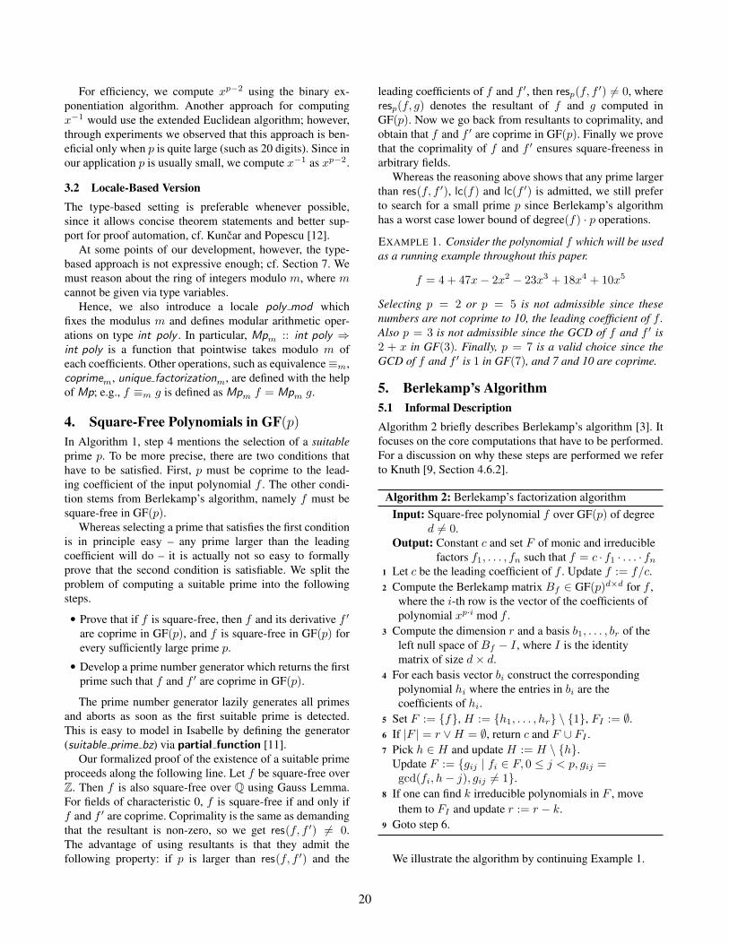
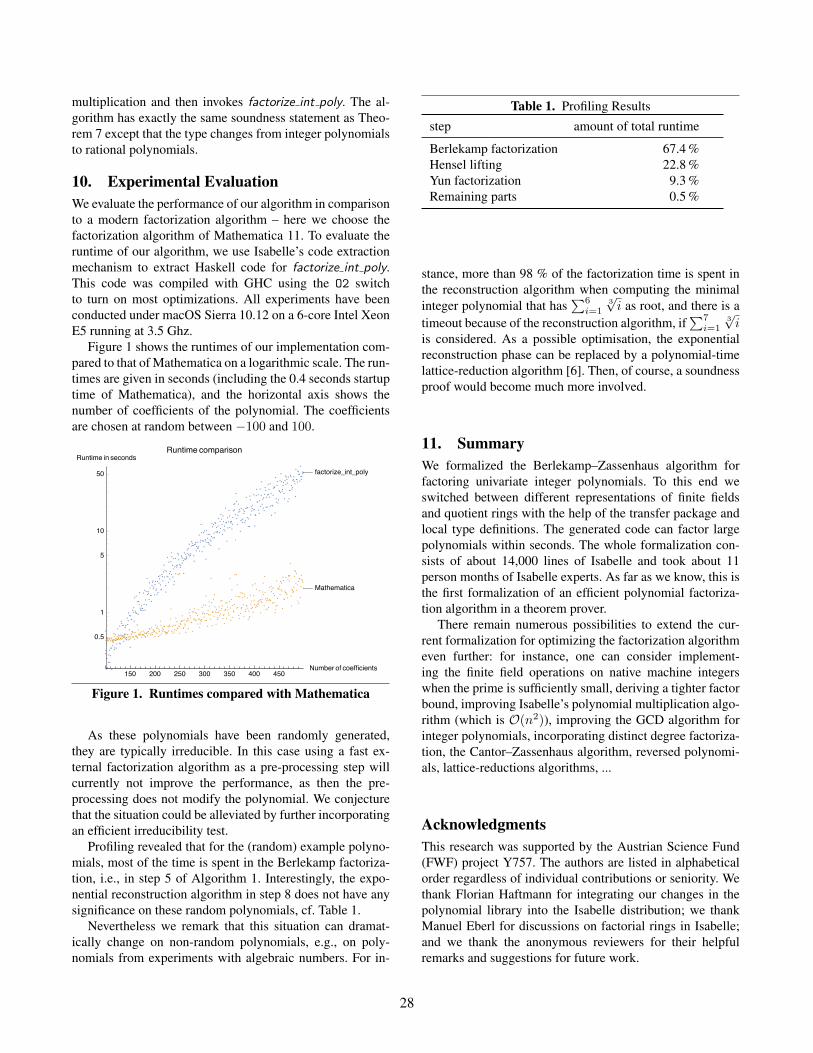
Figure 1 shows the runtimes of our implementation com-pared to that of Mathematica on a logarithmic scale. The run-times are given in seconds (including the 0.4 seconds startuptime of Mathematica), and the horizontal axis shows thenumber of coefficients of the polynomial. The coefficientsare chosen at random between −100 and 100.

���������_���_����

�����������

��� ��� ��� ��� ��� ��� ��������� �� ������������

���

�

�

��

��

������� �� �������������� ����������

Figure 1. Runtimes compared with Mathematica

As these polynomials have been randomly generated,they are typically irreducible. In this case using a fast ex-ternal factorization algorithm as a pre-processing step willcurrently not improve the performance, as then the pre-processing does not modify the polynomial. We conjecturethat the situation could be alleviated by further incorporatingan efficient irreducibility test.

Profiling revealed that for the (random) example polyno-mials, most of the time is spent in the Berlekamp factoriza-tion, i.e., in step 5 of Algorithm 1. Interestingly, the expo-nential reconstruction algorithm in step 8 does not have anysignificance on these random polynomials, cf. Table 1.

Nevertheless we remark that this situation can dramat-ically change on non-random polynomials, e.g., on poly-nomials from experiments with algebraic numbers. For in-

Table 1. Profiling Results

step amount of total runtime

Berlekamp factorization 67.4 %Hensel lifting 22.8 %Yun factorization 9.3 %Remaining parts 0.5 %

stance, more than 98 % of the factorization time is spent inthe reconstruction algorithm when computing the minimalinteger polynomial that has

∑6i=1

3√i as root, and there is a

timeout because of the reconstruction algorithm, if∑7i=1

3√i

is considered. As a possible optimisation, the exponentialreconstruction phase can be replaced by a polynomial-timelattice-reduction algorithm [6]. Then, of course, a soundnessproof would become much more involved.

11. SummaryWe formalized the Berlekamp–Zassenhaus algorithm forfactoring univariate integer polynomials. To this end weswitched between different representations of finite fieldsand quotient rings with the help of the transfer package andlocal type definitions. The generated code can factor largepolynomials within seconds. The whole formalization con-sists of about 14,000 lines of Isabelle and took about 11person months of Isabelle experts. As far as we know, this isthe first formalization of an efficient polynomial factoriza-tion algorithm in a theorem prover.

There remain numerous possibilities to extend the cur-rent formalization for optimizing the factorization algorithmeven further: for instance, one can consider implement-ing the finite field operations on native machine integerswhen the prime is sufficiently small, deriving a tighter factorbound, improving Isabelle’s polynomial multiplication algo-rithm (which is O(n2)), improving the GCD algorithm forinteger polynomials, incorporating distinct degree factoriza-tion, the Cantor–Zassenhaus algorithm, reversed polynomi-als, lattice-reductions algorithms, ...

AcknowledgmentsThis research was supported by the Austrian Science Fund(FWF) project Y757. The authors are listed in alphabeticalorder regardless of individual contributions or seniority. Wethank Florian Haftmann for integrating our changes in thepolynomial library into the Isabelle distribution; we thankManuel Eberl for discussions on factorial rings in Isabelle;and we thank the anonymous reviewers for their helpfulremarks and suggestions for future work.

28

References[1] C. Ballarin. Locales: A module system for mathematical

theories. J. Autom. Reasoning, 52(2):123–153, 2014.

[2] G. Barthe, B. Gregoire, S. Heraud, F. Olmedo, and S. Z.Beguelin. Verified indifferentiable hashing into ellipticcurves. In POST 2012, volume 7215 of LNCS, pages 209–228, 2012.

[3] E. R. Berlekamp. Factoring polynomials over finite fields.Bell System Technical Journal, 46:1853–1859, 1967.

[4] D. G. Cantor and H. Zassenhaus. A new algorithm for factor-ing polynomials over finite fields. Math. Comput., 36(154):587–592, 1981.

[5] J. R. Cowles and R. Gamboa. Unique factorization in ACL2:Euclidean domains. In ACL2 2006, pages 21–27. ACM, 2006.

[6] M. van Hoeij. Factoring polynomials and the knapsack prob-lem. J. Number Theory, 95(2):167–189, 2002.

[7] B. Huffman and O. Kuncar. Lifting and transfer: A modulardesign for quotients in Isabelle/HOL. In CPP 2013, volume8307 of LNCS, pages 131–146, 2013.

[8] B. Kirkels. Irreducibility certificates for polynomials withinteger coefficients. Master’s thesis, Radboud UniversiteitNijmegen, 2004.

[9] D. E. Knuth. The Art of Computer Programming, VolumeII: Seminumerical Algorithms, 2nd Edition. Addison-Wesley,1981. ISBN 0-201-03822-6.

[10] H. Kobayashi, H. Suzuki, and Y. Ono. Formalization ofHensel’s lemma. In Theorem Proving in Higher Order Log-ics: Emerging Trends Proceedings, volume 1, pages 114–118,2005.

[11] A. Krauss. Recursive definitions of monadic functions. InPAR 2010, volume 43 of EPTCS, pages 1–13, 2010.

[12] O. Kuncar and A. Popescu. From types to sets by local typedefinitions in higher-order logic. In ITP 2016, volume 9807of LNCS, pages 200–218, 2016.

[13] H. Lee. Vector spaces. Archive of Formal Proofs, 2014. URLhttp://www.isa-afp.org/entries/VectorSpace.

shtml.

[14] E. Martin-Dorel, G. Hanrot, M. Mayero, and L. Thery. For-mally verified certificate checkers for hardest-to-round com-putation. J. Autom. Reasoning, 54(1):1–29, 2015.

[15] M. Mignotte. An inequality about factors of polynomials.Mathematics of Computation, 28(128):1153–1157, 1974.

[16] A. Miola and D. Y. Yun. Computational aspects of Hensel-type univariate polynomial greatest common divisor algo-rithms. ACM SIGSAM Bulletin, 8(3):46–54, 1974.

[17] T. Nipkow, L. Paulson, and M. Wenzel. Isabelle/HOL –A Proof Assistant for Higher-Order Logic, volume 2283 ofLNCS. Springer, 2002.

[18] R. Thiemann and A. Yamada. Algebraic numbers in Is-abelle/HOL. In ITP 2016, volume 9807 of LNCS, pages 391–408, 2016.

[19] R. Thiemann and A. Yamada. Formalizing Jordan normalforms in Isabelle/HOL. In CPP 2016, pages 88–99. ACM,2016.

[20] Wolfram Research, Inc. Mathematica. Champaign, Illinois,version 11.0 edition, 2016.

[21] D. Y. Yun. On square-free decomposition algorithms. InSYMSAC 1976, pages 26–35, 1976.

[22] H. Zassenhaus. On Hensel factorization, I. J. Number Theory,1(3):291–311, 1969.

29