forecasting and levelling workload for a part feeding
TRANSCRIPT

Forecasting and levelling workload for a part feeding
system at the automotive industry

i
Date: April 2018
Author: Koen Grit, BSc
Supervisors: ing. F.J. Beverdam, MSc (Head Logistic Engineering at Scania Production Zwolle) dr. ir. J.M.J. Schutten (1st supervisor of University of Twente) dr. P.C. Schuur (2nd supervisor of University of Twente)

ii
Preface This thesis is the final part of my study Industrial Engineering and Management at the University of
Twente. In this preface I thank several persons who have helped me with the realization of this thesis
at Scania Production Zwolle.
First of all, I thank all the employees of Scania for their contribution to this research. Their enthusiastic
and open attitude contributed greatly to this research. I have experienced MZEL as a social, open and
helpful department and a fine place for writing my thesis. In particular, I thank Frank Beverdam for his
effort during the guidance of my Master Thesis.
Second, I thank Marco Schutten and Peter Schuur of the University of Twente. Their involvement and
expertise helped me during this period. Thank you for the guidance and feedback.
Finally, I thank the University of Twente. In the past five years, which consisted of three years Bachelor
and two years Master, I have learned a lot. I will carry all these experiences and insights with me in the
future. I have experienced these five years as very instructive and hope to keep having such valuable
experiences in the future.
Koen Grit, April 2018

iii

iv
Management summary At Scania, the Unit Supply Pallet process supplies full pallets with parts to multiple assembly lines on
which trucks are produced; two modes of transport are used: tugger trains and pallet trailers. This
supply process encounters variation in the workload induced by variation in the supply of requested
replenishments. Variation in workload results into overutilization of capacity during periods with high
workload and into underutilization of capacity during periods with a low workload. This problem is
caused by supplying replenishments to the assembly line, immediately after they are requested; this
is according to the Kanban system used at Scania.
By postponing the supply of replenishments from periods with a high workload to periods with a low
workload, the workload is balanced. This method copes with a stochastic demand; literature proposes
several improvements of the Kanban system, but assumes a deterministic demand. We differentiate
between three alternatives for deciding which pallets can be postponed:
1. Peak demand: replenishments can be postponed if the demand during the busiest lead time
of the planning horizon of that request is less than the bin size of the pallet. Required
information for this alternative is the bill of materials and the planned production sequence.
2. Real-time production progress: a pallet can be postponed if the part demand during the current
lead time is less than the bin size of the pallet. In addition to the first alternative, this
alternative requires accurate information about the production progress.
3. Real-time line inventory: a pallet can be postponed if the part demand during the remaining
lead time is less than the inventory level at the postponement decision. In addition to
Alternatives 1 and 2, this alternative requires accurate line inventory information.
The more accurate information is used, the more pallets can be postponed and the more balanced the
resulting workload. At the start of each supply cycle, we determine which pallets are supplied and
which are postponed. Pallets are postponed if the workload during a supply cycle exceeds a predefined
threshold: the postponement boundary.
We evaluate these alternatives by means of a simulation study. Table 1 shows the results of the
simulation study. The expected peaks, the average workload of the 20% busiest supply cycles, are
greatly reduced by postponing pallets. Furthermore, the need for extra (unplanned) capacity is
reduced by at least 69% by postponing pallets.
Table 1: Reduction of expected peak and need for extra capacity in comparison with the current situation.
Alternative
Reduction of expected peak Reduction of extra capacity needed
Tugger trains (EUR6-positions)
Pallet trailers (m3)
Number of times per day
Hours per day
1 1.59 (26.2%) 0.81 (6.8%) 2.49 (69%) 1.53 (69%)
2 1.71 (27.9%) 1.22 (10.8%) 3.30 (91%) 2.03 (91%)
3 1.86 (29.9%) 1.39 (12.2%) 3.51 (97%) 2.16 (97%)
Alternative 3 results only in a slightly better performance than the other two alternatives. Alternative
2 has a better performance than Alternative 1, which is noticeable in an additional reduction of
required extra capacity. However, this comes with the price of obtaining more accurate information
about the production progress and line inventory. For tugger trains, the differences between the three
alternatives are rather small. Therefore, we advise to implement Alternative 1 for the tugger trains.
Alternative 2 requires accurate information about the production progress and requires that
calculations are performed (real-time) at the start of each supply cycle. We suspect that the production
progress information can be obtained without much effort, but whether calculations can easily be

v
performed real-time, depends on the specific characteristics of the (ERP-)system and lies beyond the
scope of this research. If large investments or organizational changes are needed for this, we advise to
use Alternative 1 also for pallet trailers, otherwise implement Alternative 2.
We advise to use an intermediate computer program for deciding which pallets are postponed and
which are supplied. Otherwise, the logistical process becomes too complex and error-prone, as printed
transport orders have to be sorted manually. The computer system calculates which pallets can be
postponed during the night run of the ERP-system. It has to retrieve the bill of materials and the
planned production sequence from the ERP-system to determine which pallets can be postponed.
Incoming requests of the empty pallets are received and the system buffers the requests that are
postponed. Transport orders are printed for the replenishments that are supplied. For Alternative 1,
the intermediate system calculates the peak demand during the night run, whereas for Alternative 2,
calculations for the demand during the remaining lead time have to be performed real-time at the
start of each supply cycle.
The utilisation of the planned capacity is not improved by postponing replenishments, as the average
workload is not influenced by it and the current supply zones are kept the same. For that reason, we
propose two Mixed Integer Programming (MIP) model that (re)allocate inventory locations to the
tugger train and pallet trailer supply zones (parts belonging to the same supply zone are supplied in
the same supply cycle). To reduce the problem size, locations are combined into clusters that are
supplied together.
Either up to two (out of three) tugger trains can be eliminated or one tugger train and one (out of nine)
pallet trailer zone can be eliminated by means of the reallocation of the location clusters to supply
zones resulting from the MIP-models. This reduction is based on the production rate in February 2018.
The reallocation itself also comes with a cost, among others the visualisation of the supply zones needs
to be replaced. Moreover, a proposed reallocation has to be approved by the relevant logistical
departments. Therefore, we advise to only reallocate inventory locations if significant cost savings
(eliminating supply zones) can be achieved. Once or twice a month, it should be checked whether the
current allocation still suits the current demand pattern.
Furthermore, we advise to convert the proposed models into a computer-aided decision tool, such
that hard-to-model-considerations can be taken into account into the allocation of inventory locations
to supply zones. Another advantage of this is that a more detailed allocation can be made without
having troubles of solving a too large problem instance. This proposed tool can be used in addition to
the MIP-models; we advise to use the MIP-models to investigate where potential capacity
improvements can be found and to use the tool such that the allocation proposed by the MIP-models
can be converted into an allocation that is feasible in practice.

vi
Table of Contents 1. Introduction ..................................................................................................................................... 1
1.1 Reason of research .................................................................................................................. 1
1.2 Core problem ........................................................................................................................... 1
1.3 Research goal .......................................................................................................................... 3
1.4 Research scope ........................................................................................................................ 3
1.5 Research questions and approach .......................................................................................... 4
2. Current situation ............................................................................................................................. 5
2.1 Production process .................................................................................................................. 5
2.2 Part feeding process ................................................................................................................ 6
2.3 Production planning process ................................................................................................... 8
2.4 Workforce scheduling process ................................................................................................ 9
2.5 Workload at Unit Supply Pallets .............................................................................................. 9
2.6 Capacity utilisation ................................................................................................................ 12
2.7 Return flow sequencing and kitting ...................................................................................... 13
2.8 Conclusions ............................................................................................................................ 13
3. Literature review ........................................................................................................................... 15
3.1 Assembly line ......................................................................................................................... 15
3.2 Part feeding process .............................................................................................................. 16
3.3 Improving the Kanban system ............................................................................................... 17
4. Solution design .............................................................................................................................. 21
4.1 Alternative solutions ............................................................................................................. 21
4.2 Alternative 1: forecasting peak demand ............................................................................... 22
4.3 Alternative 2: real time production progress ........................................................................ 25
4.4 Alternative 3: real time production progress and line inventory .......................................... 26
4.5 Comparison of alternatives ................................................................................................... 27
4.6 Levelling workload by postponing replenishments ............................................................... 28
4.7 Conclusions ............................................................................................................................ 31
5. Simulation model .......................................................................................................................... 33
5.1 Model description ................................................................................................................. 33
5.2 Input of the model ................................................................................................................. 35
5.3 Output of the model .............................................................................................................. 36
5.4 Model verification and validation ......................................................................................... 37
5.5 Experimental design .............................................................................................................. 38
5.6 Results of simulation study ................................................................................................... 39
5.7 Conclusions ............................................................................................................................ 44

vii
6. Rebalancing supply zones .............................................................................................................. 47
6.1 Why rebalancing supply zones? ............................................................................................ 47
6.2 Alternatives for rebalancing supply zones ............................................................................ 48
6.3 MIP-model description .......................................................................................................... 48
6.4 Model description – Generating tugger train tours .............................................................. 51
6.5 Model description – Allocating supply locations................................................................... 54
6.6 Results of MIP-models ........................................................................................................... 57
6.7 Conclusions ............................................................................................................................ 60
7. Conclusions and recommendations .............................................................................................. 61
7.1 Conclusions ............................................................................................................................ 61
7.2 Recommendations of proposed solutions ............................................................................ 62
7.3 Recommendations for further research ................................................................................ 64
8. References ..................................................................................................................................... 65
A. Terminology and abbreviations ..................................................................................................... 67
B. Flowchart of postponement decision in simulation model .......................................................... 68
C. Simulation model validation: goodness-of-fit tests ...................................................................... 69
D. Warm-up period – Welch’s graphical method .............................................................................. 70
E. Statistical techniques for analysing simulation results ................................................................. 73
F. Results of simulation model .......................................................................................................... 74

1
1. Introduction This report is the result of my Master Project at Scania Production Zwolle (SPZ). This Master project is
the final project of my study Industrial Engineering and Management. SPZ assembles trucks on two
assembly lines. This research focuses on controlling the workload of feeding parts to the assembly lines.
Appendix A lists the terminology and abbreviations used in this research.
First, Section 1.1 addresses the reason for this research. By means of a problem cluster, we determine
the core problem (Section 1.2). Section 1.3 states the research goal and Section 1.4 the scope. Finally,
Section 1.5 defines the research questions and approach.
1.1 Reason of research Scania Production Zwolle (SPZ) is a plant that assembles trucks. On two assembly lines, a wide variety
of trucks is produced. Scania has a modular product system, which means that various types of trucks
can be produced while using a limited set of parts. The internal logistics is carried out by the
departments Factory Feeding and Line Feeding. Figure 1 shows an overview of the internal logistics.
Supplying trailers are unloaded and parts are stored in three warehouses by Factory Feeding (blue
arrow). These parts are picked from the three warehouses and delivered to the assembly lines (green
arrow); we use the term part feeding for this process. Part feeding is mainly executed by Line Feeding
and partly by Factory Feeding. Big components are transported to the assembly lines by Factory
Feeding without intermediate storage (yellow arrow). Section 2.1 gives a detailed overview of SPZ.
Figure 1: Overview of internal logistics performed by Factory Feeding (FF) and Line Feeding (LF).
Currently, the departments Factory Feeding and Line Feeding struggle with controlling the workload
encountered at their logistical processes. They struggle with determining the right number of workers
that matches the workload caused by the production at the assembly lines. However, the departments
face a varying workload, without having an accurate method for predicting the future workload and
the corresponding number of personnel. Furthermore, nearly no workload-related figures are available
at Scania. At Scania, the need exists for more detailed workload and productivity figures, such that
continuous improvement goals can be set more precisely.
1.2 Core problem Figure 2 shows the problem cluster by which we determine the core problem. The problem cluster
shows the cause-effect relationships of the problems at Factory and Line Feeding. The next paragraph
explains these relationships. The core problem can be identified by going back in the problem cluster
(Heerkens and Van Winden, 2012). Going back means finding the problem that does not have any
preceding causes. Causes that are hard to change or with little impact are no core problems. The red
marked boxes show problems that are hard to influence. The yellow marked boxes show problems
with little impact on the other problems. The blue marked boxes show potential core problems.
FF LF (+FF)
FF

2
8. Peaks in workload at unloading trucks
are elevated
9. Workload associated figures are
mostly unavailable
18. Unable to control workload
11. Unclear where and when peaks in workload appear
15. Helping out other team members is not
always possible
14. Members of the same team are
working at different physical locations
13. Team members are not trained for all tasks within a team
10. No forecast of workload is available
16. Not possible to adjust personnel to workload on short
notice
6. Late arrival of supplying trailers
7. Trailers are loaded incorrectly
12. Temporary employees need to be requested 1.5 weeks
in advance.
5. Peaks in workload at feeding parts to the line
3. Peaks in replenishment requests by production
4.Replenishment requests are immediately supplied to the
line because of Kanban system
1. Deviations in moment of replenishment request
due to human action
2. The moment a pallet empties is stochastic.
17. Unable to match personnel to encountered
workload
Figure 2: Problem cluster of workload control at Factory and Line Feeding.
Scania is unable to control the workload at Factory and Line Feeding (problem (18) in Figure 2). A
fluctuating workload can be approached in two ways. First, the available capacity can be adjusted to
the encountered workload, i.e. capacity is increased in periods of high workload and decreased in
periods with low workload. A prerequisite for matching the capacity with the workload is being able
to forecast the workload. Second, workload can be controlled by levelling it; by levelling the workload,
the need for adjusting capacity disappears. These two solution approaches are also present in the
problem cluster (Figure 2). Problems (1) to (8) are causing a non-levelled workload. The replenishment
requests have a fluctuating pattern (3). A varying number in requests results in a varying workload as
Scania uses a Kanban system for these requests (4): when a pallet empties a request is made for the
immediate supply of a full. In other words, peaks in replenishment requests result in peaks in workload
at the part feeding process. The workload encountered at unloading trucks is mostly caused by external

3
causes: (6) and (7). These problems are no core problems as they are hard to influence. Currently,
matching capacity with the encountered workload is not possible due to problems (9) to (17). It is
unclear where and when peaks in workload appear, as no forecast method of the workload exists (10).
This workload is mainly affected by the number of replenishments per supply cycle (Chapter 2
describes the processes in more detail). Next to that, nearly no figures associated with workload are
available at Scania (9). Problems (12), (13) and (14) restrict the adjustment of personnel on short notice.
Five potential core problems remain from Figure 2:
1. (1) Human action causes deviations in the moment of replenishment requests.
2. (2) The moment a pallet empties is stochastic.
3. (4) Replenishment requests are immediately supplied due to Kanban system.
4. (9) Workload associated figures are mostly unavailable.
5. (10) No forecast of workload is available.
From these problems, the core problem is the problem with the highest expected potential. By tackling
the first, second and third problem, the workload at the part feeding system can be levelled. By
addressing the fourth and fifth problem, capacity can be matched with the varying workload. When
matching capacity with the workload, additional capacity is (temporarily) needed to overcome the
peaks. Therefore, we prefer levelling the workload as the peaks are lowered, and thereby also the
needed capacity. The potential of the first problem is limited, as the request pattern will still vary due
to problem (2) in the problem cluster. Solving this second problem is possible by obtaining more
information about when a pallet empties, for example information about the line inventory. Nowadays,
the workload is directly linked to the replenishment requests as requested pallets are immediately
supplied to the line. By reducing this link, levelling the workload at part feeding can be achieved.
Summarizing the identified core problem is:
1.3 Research goal The research goal is to find adaptations in the process design of Unit Supply Pallets that level the
workload at internal logistics. A part of this method is to forecast the workload based on the production
planning.
1.4 Research scope Figure 1 shows an overview of the internal logistics as performed by Factory Feeding and Line Feeding.
We focus on the part feeding process (green arrow in Figure 1) as this process is influenced by internal
factors. Therefore, Scania has more control over the part feeding process than over the other two
processes in Figure 1; those are mainly influenced by external factors.
Supply methods At Scania, the supply of parts to the assembly lines is classified in four categories. This section briefly
describes these four methods and Chapters 2 and 3 further describe these methods.
1. Unit Supply: the supply of highly consumed parts, which are supplied in pallets or bins.
2. Batch Supply: a rack containing a set of batches is offered to the assembly line. Here we define
a batch as multiple items of the same part. Each batch has its own up-to-order-level. After a
fixed time, these batches are refilled.
3. Kitting: different parts are picked together for one or multiple chassis.
The current Kanban replenishing system directly links the current workload at part feeding to
the replenishment pattern.

4
4. Sequencing: the supply of parts that do not fit in the other three methods due to low
consumption rate or due to the size of the parts, e.g. axles and tires. Individual parts are
offered to the line in correspondence to the production sequence.
In this research we focus on Unit Supply, while keeping in mind the applicability to the other supply
methods. We focus on this supply method, as it perceives a fluctuating workload. Next to that it has
several aspects that can be adapted to level the workload. Unit Supply has two sub-processes: Pallets
and Bins (see Chapter 2). In consultation with the stakeholders, we choose for focusing on Unit Supply
Pallets; we still investigate Unit Supply Bins as it bears resemblances with Unit Supply Pallets.
1.5 Research questions and approach This section defines the research questions for this research and how we approach these questions.
1. What is the current situation at the internal logistics regarding the workload?
Chapter 2 gives an outline of the current situation with regard to the workload. Sub-questions
are:
• What is the production process at Scania?
• What is the current internal logistics process?
• What is the current production planning process?
• What is the current workforce scheduling process?
• What is the current variation in workload and personnel capacity?
We investigate the processes by interviewing different actors of the processes and by
shadowing operators and team leaders at internal logistics. In this way, we are able to pinpoint
critical process steps with regard to the workload. The second step is to quantify the
encountered workload. Most required data is available in the ERP-system, e.g. number of picks
per aisle, number of required parts per day. We determine the workforce size by means of the
internal personnel system.
2. Which methods are described in the literature for predicting and controlling workload for
feeding parts to production lines?
Chapter 3 positions this research in a conceptual framework based on literature. Chapter 3
investigates literature on predicting and controlling workload. Among others, it addresses
several problems in literature that have similarities to our problem. Furthermore, it addresses
solutions for levelling the workload at the part feeding system.
3. How can the workload at internal logistics be forecasted as a function of a production plan and
how much (personnel) capacity is needed as a function of the workload?
Chapter 4 proposes a method for forecasting the workload at part feeding. This method is
needed for answering the next research question. Based on insights obtained from the current
situation analysis, we determine a method for forecasting the workload. The proposed method
also has to be validated. During the creation of the forecasting method, close cooperation with
the end-users is required to create a method that is practically useful.
4. What adaptations at the Unit Supply Pallets process cause a levelled workload?
Based on the current situation analysis, we determine adaptations of the Unit Supply
processes that level the workload. Chapter 4 proposes a method for levelling the workload.
This method incorporates the forecasting method determined by the third research question.
Chapter 5 evaluates these adaptations by means of a simulation model. Chapter 6 proposes
two MIP-models for rebalancing the workload at Unit Supply Pallets.

5
2. Current situation This chapter analyses the current situation at SPZ. First, it describes several processes at SPZ that are
relevant for the workload at the part feeding processes. After that, it presents figures to quantify the
encountered workload and the utilisation of capacity. We use this analysis to define solution proposals
for balancing the encountered workload.
Section 2.1 gives an overview of SPZ and its production process. Section 2.2 first gives an overview of
the different supply methods at SPZ. After that, the section goes into detail on the focus of this research:
the supply method Unit Supply Pallets (USP). Section 2.3 describes how the production sequence is
determined at SPZ and Section 2.4 explains the workforce scheduling process. Section 2.5 quantifies the
workload encountered at USP. Section 2.6 investigates the capacity utilisations at USP. Section 2.7 goes
into detail into the return flow of pallets. Section 2.8 makes concluding remarks on the current situation
analysis and proposes several adaptation areas for balancing the workload at USP.
2.1 Production process Figure 3 shows a map of Scania Production Zwolle (SPZ). SPZ has an assembly hall that contains two
assembly lines. Parts are stored in Warehouses A, B and C. Warehouse A is used for the Unit Supply of
pallets (Section 2.2 further explains the supply methods). Warehouse B is divided over two physical
stores, B.a and B.b. Warehouse B is a warehouse in which batch picking and kitting takes place.
Warehouse C is a warehouse in which kitting takes place. After consumption of parts on the lines, the
pallets are broken down (pallet edges are removed from the pallet bottom), before sending the
packaging back to the suppliers. Across the street, Scania Logistics Netherlands (SLN) is located. This is
a separate company in the Scania Group. Among others, SLN is responsible for replenishing bins with
small-sized parts (Unit Supply of bins).
Figure 3: Overview of Scania Production Zwolle (SPZ). The purple area is part of Scania Logistics Netherlands B.V. (SLN), a separate company of the Scania Group. SLN is located across the street. Parts are stored in the three warehouses (A, B, C).
The production process starts with constructing the frame of the truck. Then the truck is assembled on
one of the two assembly lines. These assembly lines are divided into consecutive workstations. Next
to the two assembly lines, many pre-assembly stations are present. Pre-assembly is used such that a
truck needs less time on the assembly line. Figure 3 indicates two major pre-assembly stations: the
engine and cabin completion; the other pre-assembly stations are not shown in the figure. Each
workstation and pre-assembly station has its own inventory of parts. The highly consumed parts are
kept on stock at the workstations, mostly according to the two-bin principle. Lowly consumed parts
are offered to the line just-in-time on racks or in pallets. Parts for the assembly lines and the pre-
assembly stations are fed by the departments Line Feeding and Factory Feeding.

6
Tact time Each assembly line has its own tact time: the time between the completion of two consecutive trucks.
This means that every tact time, the chassis moves to the next workstation. The tact time is based on
the demand for trucks. The production process and many internal logistic processes are linked to this
tact time. Line workers can be divided into regular workers and floaters. Each worker has its own role,
which consists of several tasks. Tasks are divided over the regular workers, such that a worker can
finish the tasks within the tact time. Each tact time, regular workers repeat their tasks. The more
complex trucks require more tasks and some of them cannot be performed within the tact time by the
regular workers. Floaters support the regular workers with these tasks, i.e. some tasks are performed
by floaters instead of the regular workers. A floater is not restricted to a single workstation but receives
a schedule that shows which tasks to perform when on which chassis.
2.2 Part feeding process First, this section describes the supply methods used at SPZ. Afterwards, it explains the supply method
Unit Supply more thoroughly as the scope of research lies at Unit Supply. Section 3.2 links the supply
methods to the literature. The choice between these supply methods is based on inventory limitations
at the assembly line, consumption rate and size of the parts.
• Unit Supply (US): at this supply method no repackaging of parts takes place. Highly consumed
parts are offered to the line in pallets or bins. Replenishments take place according to the two-
bin principle. After this bullet list, we further describe the Unit Supply processes.
• Batch Supply: parts are offered to the assembly line on racks. Each rack contains a set of
batches; a batch contains multiple pieces of the same part. After k chassis, the batches are
refilled to predefined up-to-order levels (UOL). For example, a Batch Supply rack contains parts
A and B, with UOLs 6 and 10 respectively. After k=6 chassis the rack is taken from the line to
be refilled. Suppose that for these 6 chassis, 3 parts A and 7 parts B are consumed (some parts
are needed multiple times on the same truck). The picker then refills the rack up to 6 parts A
and 10 parts B.
• Kitting: just as with Batch Supply, different parts are picked together and offered to the
assembly line. For Batch Supply, predefined UOLs are set, but this is not the case for kitting.
The order picker receives an order picking list from the ERP-system. On this list, the parts are
listed that are needed for the next k chassis. A distinction is made between kitting and low
volume kitting. For kitting, picking is done every k chassis. Low volume kitting is not directly
linked to the tact time but picked 4-6 hours before consumption at the line.
• Sequencing: individual parts are offered to the line corresponding to the production sequence.
These are mostly big components such as axles and cabins. Also, most painted parts are
supplied by the sequencing method. Parts that are supplied by sequencing are not temporarily
stored in a warehouse and are already sorted on the production sequence by the supplier.
Unit Supply process The Unit Supply (US) is divided into US Bins (USB) and US Pallets (USP). The scope of our research is on
US Pallets, but we also address US Bins, as it has many similarities with US Pallets. Two modes of
transport are used at USP: pallet trailers (USP-PT) and tugger trains (USP-TT) (Figure 4). The inventory
locations at the assembly lines and pre-assembly stations are clustered into several supply zones. US
is a cyclical process, in which the zones are fed in a predefined schedule.
At USP, replenishments are triggered by scanning empty locations. At USP-PT, a recorder, a person,
scans empty locations according to a predefined schedule (Figure 5). The recorder scans one zone at a
time and the sequence of zones is stated in the schedule. The requested pallets are put on pallet-

7
trailers in Warehouse A. Pallet trailer drivers drive according to a predefined timetable with predefined
routes. A cycle takes 75 minutes in which three zones are supplied consecutively. At the assembly line
zones, forklift drivers put full pallets at the line and put empty pallets back on the pallet trailers. Trailers
with empty pallets are disconnected at the pallet breakdown area (Figure 3). The actual breakdown
lies beyond the scope of this research, as it is performed by a subcontractor. USP is not the only supply
method that uses pallets; low volume kitting and sequencing also uses pallets for some parts. The full
pallets of kitting and sequencing are brought to the line by forklift drivers, but the return flow of these
pallets is incorporated in the USP-flow, i.e. the empty pallets of USP, sequencing and kitting are put
together on pallet-trailers.
Figure 4: Different transport vehicles. From left to right, an empty pallet trailer (PT); a tugger train (TT) with pallets on blue trolleys and a pallet truck on which racks with bins are put.
USP-TT (tugger trains) differ on several points from USP-PT (Figure 6). As pallets are put on trolleys, no
forklifts are needed to exchange full and empty pallets at the assembly line. Scanning is also done by
the train driver instead of a separate recorder. The handling at the pallet breakdown area differs: pallet
trailers are disconnected and left behind, whereas train drivers have to wait while the empty pallets
are unloaded from the trolleys. Just like USP-PT, three zones are supplied in one cycle: however, the
cycle time is 90 minutes instead of 75 minutes.
Figure 5: Part feeding process of USP by means of pallet trailers.
Unit Supply Pallets – pallet trailers
Rec
ord
erFo
rklif
t d
rive
rs
War
ehou
se A
Palle
t tr
aile
r d
rive
rsFo
rklif
t d
rive
rs a
t zo
nes
Recorder starts checking cycle
Replenishment orders are requested for empty locations at
assembly lines
Requested pallets are taken out of the
warehouse and put onto pallet-trailers
Empty pallets are put on
pallet-trailers
Pallet-trailers with empty pallets are
driven to pallet breakdown
Pallet-trailers are driven to
zones near the assembly line
Pallets are put at the line by forklift trucks
Pallet-trailers with empty pallets are
disconnected at pallet breakdown
8
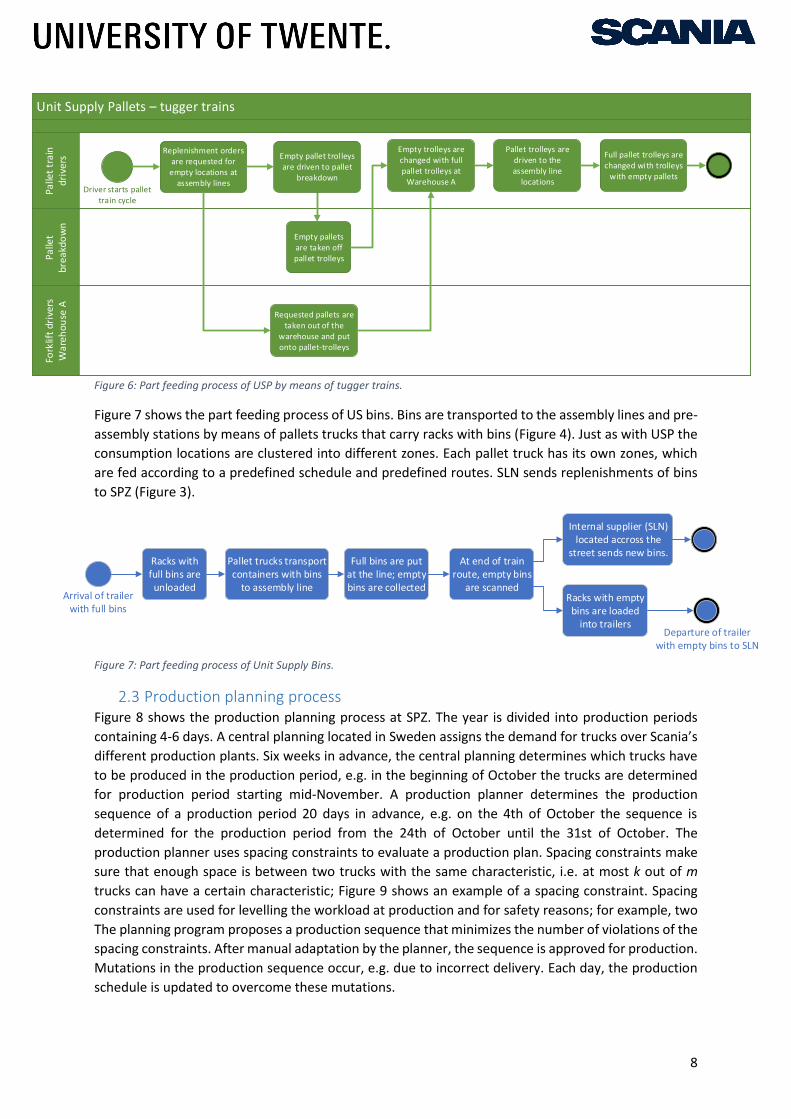
Figure 6: Part feeding process of USP by means of tugger trains.
Figure 7 shows the part feeding process of US bins. Bins are transported to the assembly lines and pre-
assembly stations by means of pallets trucks that carry racks with bins (Figure 4). Just as with USP the
consumption locations are clustered into different zones. Each pallet truck has its own zones, which
are fed according to a predefined schedule and predefined routes. SLN sends replenishments of bins
to SPZ (Figure 3).
Figure 7: Part feeding process of Unit Supply Bins.
2.3 Production planning process Figure 8 shows the production planning process at SPZ. The year is divided into production periods
containing 4-6 days. A central planning located in Sweden assigns the demand for trucks over Scania’s
different production plants. Six weeks in advance, the central planning determines which trucks have
to be produced in the production period, e.g. in the beginning of October the trucks are determined
for production period starting mid-November. A production planner determines the production
sequence of a production period 20 days in advance, e.g. on the 4th of October the sequence is
determined for the production period from the 24th of October until the 31st of October. The
production planner uses spacing constraints to evaluate a production plan. Spacing constraints make
sure that enough space is between two trucks with the same characteristic, i.e. at most k out of m
trucks can have a certain characteristic; Figure 9 shows an example of a spacing constraint. Spacing
constraints are used for levelling the workload at production and for safety reasons; for example, two
The planning program proposes a production sequence that minimizes the number of violations of the
spacing constraints. After manual adaptation by the planner, the sequence is approved for production.
Mutations in the production sequence occur, e.g. due to incorrect delivery. Each day, the production
schedule is updated to overcome these mutations.
Unit Supply Pallets – tugger trains
Fork
lift
dri
vers
W
areh
ouse
AP
alle
t b
rea
kdo
wn
Pal
let
trai
n
dri
vers
Requested pallets are taken out of the
warehouse and put onto pallet-trolleys
Empty trolleys are changed with full pallet trolleys at
Warehouse ADriver starts pallet
train cycle
Replenishment orders are requested for empty locations at
assembly lines
Pallet trolleys are driven to the assembly line
locations
Full pallet trolleys are changed with trolleys
with empty pallets
Empty pallets are taken off pallet trolleys
Empty pallet trolleys are driven to pallet
breakdown
Arrival of trailer with full bins
Racks with full bins are unloaded
Pallet trucks transport containers with bins
to assembly line
Full bins are put at the line; empty bins are collected
At end of train route, empty bins
are scanned
Internal supplier (SLN) located accross the
street sends new bins.
Racks with empty bins are loaded
into trailersDeparture of trailer
with empty bins to SLN

9
Assigning demand to production periods
Manual adaptation of proposed sequence
Mutations in production sequence
Planning program proposes production
sequence
6 weeks 20 days 20 days 0-20 days
Figure 8: Production planning process.
Figure 9: This sequence has one violation for the spacing constraint: max. 1 out of 3 trucks may have a coloured side skirt.
2.4 Workforce scheduling process The internal logistics is performed by the two departments Line Feeding and Factory Feeding. These
two departments combined are divided into five supervisor areas. A supervisor area is divided into
several team leader areas, which contain 5-10 operators each (Figure 10). Each operator has its own
role, also called a standard. This standard prescribes which tasks an operator needs to perform. Next
to a fixed workforce, additional temporary workers can be requested by the supervisors. Requests
have to be made 1.5 week in advance. Currently additional workforce is requested based on
experience and occurred workload peaks. Also, for some areas, concise forecasts are available for the
number of picks per day; these forecasts are used for determining the needed workforce.
Figure 10: Hierarchical structure of a supervisor area.
2.5 Workload at Unit Supply Pallets Daily, about 1900 pallets are replenished by the Unit Supply Pallets process. Figure 11 shows the
number of replenishments per day (orange line); besides that, the index of produced trucks is plotted
(blue line). The index is based on the number of trucks produced at the 1st of November, 2017, i.e. on
the 7th of November 20% more trucks are produced than on the 1st of November. This figure shows
that the number of replenishments heavily depends on the number of trucks produced. Although the
number of replenishments per day fluctuates, we conclude that the daily demand at pallets at
production is stable, as there is little variation in the number of pallets per produced truck. Differences
in number of produced trucks depend among others on line downtime or work in overtime.
Operators
Teamleaders
Supervisor

10
Figure 11: Daily number of replenishment requests and number of produced trucks. Source: Scania's ERP-system
Scania’s production plant is divided into 9 pallets trailer zones and 9 tugger trains zones. Each pallet
trailer/tugger train supplies three zones, i.e. Tugger train zones 1A, 1B and 1C are supplied by a single
tugger train. Figure 12 shows the sizes of the different supply zones at Scania; we measure the size of
a zone by the daily number of replenished pallets and by the total volume of the replenished pallets.
In this figure, the return flows of sequencing and kitting are not taken into account; Section 2.7
addresses this flow. Tugger trains can carry less pallets than pallets trailers, which is also visible in the
figure. We make a remark on Tugger train 3: in November 2017, one of the two assembly had been
converted for a new truck generation. Due to this, few replenishments have been made for the zones
that are supplied by Tugger train 3. Based on Figure 12, we conclude that variation in number and
volume is noticeable between the different zones.
Figure 12: Sizes of Unit Supply Pallet zones based on the daily number and volume of pallet replenishments. Figures are based on December 2017. Source: Scania's ERP-system.
0
500
1000
1500
2000
2500
0%
20%
40%
60%
80%
100%
120%1
-11
-20
17
2-1
1-2
01
73
-11
-20
17
6-1
1-2
01
77
-11
-20
17
8-1
1-2
01
79
-11
-20
17
10
-11
-20
17
13
-11
-20
17
14
-11
-20
17
15
-11
-20
17
16
-11
-20
17
17
-11
-20
17
20
-11
-20
17
21
-11
-20
17
22
-11
-20
17
23
-11
-20
17
24
-11
-20
17
27
-11
-20
17
28
-11
-20
17
29
-11
-20
17
30
-11
-20
17
1-1
2-2
01
74
-12
-20
17
5-1
2-2
01
76
-12
-20
17
7-1
2-2
01
78
-12
-20
17
9-1
2-2
01
71
1-1
2-2
01
71
2-1
2-2
01
71
3-1
2-2
01
71
4-1
2-2
01
71
5-1
2-2
01
71
6-1
2-2
01
71
8-1
2-2
01
71
9-1
2-2
01
72
0-1
2-2
01
7
Pal
lets
rep
len
ish
ed
Ind
ex p
rod
uce
d t
ruck
sCurrent workload of Unit Supply Pallets
0
50
100
150
200
250
300
Unit Supply Pallet zones
Daily number of replenishments Daily volume of replenishments (m3)

11
Next to variation between zones, also variation within a zone is noticeable. We demonstrate this for a
specific zone: Pallet trailer 2C. A USP-PT-zone is replenished 11-12 times a day, whereas USP-TT-zones
are replenished 9-10 times a day. Figure 13 shows that the number of replenishments per
replenishment cycle varies. Figure 14 compares the number of replenishment requests with the pallet
usage by production. Based on the product structure, Scania’s ERP-system determines which parts are
needed for each truck at each assembly workstation; when these parts are needed is based on the
planned production times. This planned pallet usage is compared with the actual replenishment
requests. We conclude that the variation in pallets usage by production is less than the variation in
replenishment requests.
Figure 13: Empirical probability histogram of replenishments in each cycle. Data from November and December 2017 for Zone Pallet Trailer 2C. Source: Scania’s ERP-system.
Figure 14: Comparison between the number of replenishments in a cycle and the planned usage of pallets at production for Pallet Trailer 2C. Source: Scania’s ERP-system.
The conclusions made for this specific zone are also applicable to the other zones. For all zones, the
variation is less for the planned pallet usage than for the replenishments requests in each cycle (Figure
15). We conclude that the pallet demand by production is more stable than the replenishing process
itself. This difference has several causes. First, the moment a pallet is empty is influenced by
coincidence, especially for low-consuming locations. We illustrate this by an example: a pallet contains
5 parts and on each truck 1 part is required. Then the usage is stable, 0.2 pallet per tact time, but
0,0%
2,0%
4,0%
6,0%
8,0%
10,0%
12,0%
8 9 10 11 12 13 14 15 16 17 18 19 20 21 22 23 24 25 26 27 28 29 30 31 32
Number of replenishments per cycle
Empirical probability histogram of number of replenishments per cycle - Pallet trailer 2C
0
5
10
15
20
25
30
1 2 3 4 5 6 7 8 9 10 11
Pal
lets
Cycle number
Pallet usage and replenishments - Pallet trailer 2C
Number of replenishmentrequests in cycle
Pallet usage by production

12
variation occurs in the replenishments: at 1 tact time, a replenishment is made and the other 4 tact
times not. Second, deviations occur in the replenishment trigger. A request should be made for an
empty location, but sometimes replenishments are made for nearly-empty locations. This has a
negative side effect that there is no space for the replenished pallet in case the nearly-empty location
is still not empty.
When we compare Figure 15 with Figure 12, we conclude that the bigger zones have less variation
than the smaller zones. Here the law of large numbers is present: the more pallets a zone contains the
more stable the number of replenishments per cycle. The law of large numbers states that the average
of a large number of random variables tends to fall close to the expected value (Smith and Kane, 1994).
This is in line with the first notion in the previous paragraph.
Figure 15: Coefficient of variation of the number of replenishments and the planned pallet usage by production for December 2017. Source: Scania’s ERP-system.
2.6 Capacity utilisation A fluctuating workload has a negative effect on the capacity utilisation. First, extra capacity is needed
to cope with peaks in workload. This assistance is provided by team leaders and troubleshooters;
troubleshooters are operators at Scania whose task is supporting other operators when needed. On
the other hand, capacity is underutilised in periods with a low workload. In this section, we investigate
the capacity utilisation of Unit Supply Pallets. We address the loading capacity of the pallet trailers and
tugger trains.
The loading capacity of a pallet trailer (PT) is 12 m3. In a pallet trailer, pallets can be stacked. However,
due to the shape of the pallets and due to restrictions in stacking pallets, this 12 m3 cannot be fully
utilised. At Scania, calculations are made with an effective loading capacity of 10 m3. Each pallet trailer
supply zone is replenished 11.33 times a day. Each cycle, two pallet trailers are sent to each supply
zone. This means that per cycle 20 m3 is available as loading capacity; the daily capacity is 227 m3. The
capacity utilisation is calculated as the daily volume of the replenished pallets (see Figure 12) divided
by the daily capacity. The average capacity utilisation of the pallet trailers is 48%. The bigger zones, PT
3A and PT 1C, have a utilisation of 75% and 69% respectively, whereas the smaller zones, PT 1A and PT
2B, have a utilisation of respectively 17% and 15%. These figures are calculated for the supply flow;
the capacity utilisation of the return flow differs, as Section 2.7 explains.
00,10,20,30,40,50,60,70,80,9
1
Co
effi
cien
t o
f va
riat
ion
Coefficient of variation
C.V. replenishment requests C.V. planned pallet usage by production

13
A tugger train (TT) can transport two sizes of pallets: EUR 1- and EUR 6-pallets. The height of a pallet is
irrelevant for a tugger train capacity as pallets cannot be stacked (see Figure 4). EUR 1-pallets, also
called EUR(O)-pallets, are standard sized pallets (Epal-pallets.org, 2018); EUR 6-pallets are half the size
of EUR-pallets. A tugger train has nine positions for EUR 6-pallets. On two EUR 6-pallet positions, one
EUR-pallet can be placed, e.g. a tugger train can transport two EUR-pallets, which use four positions,
and five EUR 6-pallets. Each zone is supplied 9.67 times a day; the daily capacity is 9.67*9 = 87 EUR 6-
pallets positions per zone. Figure 12 shows the daily number of replenishments per zone. This number
of pallets is translated into number of EUR 6-units, i.e. each EUR-pallet is counted twice and each EUR
6-pallet once. For example, zone TT 1A supplies 42.1 pallets a day of which 16.5 are EUR-pallets. Hence
the zone supplies 16.5 x 2 + 25.7 = 58.7 EUR 6-units a day. Then the capacity utilisation is 58.7/87=67%.
The average capacity utilisation of Tugger Trains 1, 2 and 3 are respectively 53%, 62% and 13%.
2.7 Return flow sequencing and kitting As mentioned in Section 2.2, pallets are also used by the supply methods sequencing and kitting. These
pallets are offered to the line by means of forklifts. After consumption, the empty pallets are put on
the pallet trailers of USP and together transported to the pallet breakdown. In other words, the return
flow of the pallets of sequencing and kitting is merged at the USP-return flow. Consequently, the
capacity utilisation of the supplying pallet trailers deviates from that of the returning pallet trailers.
The daily total volume of the return flow of sequencing and kitting is about 600 m3 (the daily total USP-
flow is 1045 m3). 80% of this 600 m3 consists of sequencing pallets; the other 20% of kitting. For three
pallet trailer zones the effect of sequencing (and kitting) is noticeable: zones PT 1A, PT 2B and PT 4B.
This supply method consists of fifth wheels, silencers and coloured parts. For these zones, the
additional daily return flow is 147 m3, 197 m3 and 119 m3 respectively. Especially for zones PT 1A and
PT 2B, the imbalance between the supply and return flow is noticeable.
2.8 Conclusions At Scania, variation occurs in the replenishment pattern of Unit Supply Pallets. Variation occurs
between supply zones and between replenishment cycles. Due to this variation additional capacity is
needed to overcome peaks in workload. At Scania, peaks are overcome with assistance of team leaders
and troubleshooters. Due to this, these employees have less time for their regular activities. As (extra)
capacity is needed to cope with the varying workload, also underutilisation of capacity takes place;
capacity is underutilised in the periods of lower workload. At Scania, tugger trains and pallet trailers
have an average capacity utilisation of 67% and 48%. However, still situations occur in which pallets
cannot be supplied by means of the regular capacity. When workload is perfectly balanced, capacity
should match the average workload; a varying workload requires more capacity (even if the average
workload is the same), as capacity should also cope with periods of higher workload. Hence, with a
levelled workload, less capacity is needed or in other words more pallets can be supplied with the
current capacity.
Levelling workload means that the variation in the supply of replenishments per supply cycle needs to
be reduced. Figure 16 distinguishes three improvement areas that could contribute to a reduction of
variation. First, the variation in replenishments has its origin in the demand pattern by production.
Based on Figure 14, we conclude that the demand pattern is more stable than the replenishment
pattern. Also, the number of replenished pallets per produced truck is stable. This demand pattern is
influenced by the production planning. We conclude that the potential improvement by changing the
current production planning is limited, as the demand pattern of Unit Supply Pallets is already fairly
stable. Therefore, we focus on the other two areas.

14
Figure 16: Three potential areas for levelling workload at Unit Supply.
The second improvement area is the replenishment request triggering mechanism. At Scania,
replenishments are cyclically requested for empty inventory locations. As said in Section 2.5, variation
in the requests occurs due to human action and is caused by the stochastic behaviour of in which
supply cycle a pallet empties.
The third area comprises how replenishments requests are processed. According to Scania’s current
process design, pallets are replenished immediately after they are requested. However, not all pallets
are already needed in that replenishment cycle and could be postponed to periods with a lower
workload. A drawback of postponing requests is a possible stock out at the assembly line. This should
be avoided as a stock out could lead to line stoppage. In Chapter 4 we propose a method to postpone
replenishment requests, while avoiding line stoppage.
Postponing requests is a method to reduce variation that is based on the risk pooling principle: high
demand in one location is offset by low demand in another location. By postponing (or advancing)
requests risk pooling takes place over time; a quiet period is offset by a busy period. This risk pooling
effect can also be utilised by aggregating routes/supply zones (risk pooling over areas). Nowadays,
each tugger train or pallet trailer has its own routes/supply zones and supporting each other is not
incorporated in the process design. Therefore, the risk pooling effect is not utilised at Scania. This is
noticeable as smaller supply zones encounter a more varying workload. Due to their lower capacity,
tugger trains supply less pallets than pallet trailers. Hence, risk pooling is mostly beneficial to the
utilisation of tugger trains.

15
3. Literature review This chapter investigates literature relevant to our research. It positions this research in a conceptual
framework based on recent literature. Furthermore, this chapter discusses resemblances between
problems found in literature and the problem that Scania is facing.
This chapter first describes what a mixed-model assembly line is and which planning problems occur at
mixed-model assembly lines (Section 3.1). Section 3.2 positions Scania’s part feeding process in supply
methods that are discussed in literature. Section 3.3 gives an overview of solutions proposed in
literature that improve the efficiency of the part feeding system. Moreover, it links the proposed
solutions with the situation at Scania.
3.1 Assembly line Assembly lines are used in the automotive industry for low costs (Golz et al., 2012; Boysen et al., 2015) .
Originally these assembly lines were single-model: only one model can be produced on the assembly
line. Due to higher customer requirements, nowadays mostly mixed-model assembly lines are used.
These lines are capable to produce a large variety of vehicles due to their modular design.
Consequently, a large variety of parts is needed for production. The difference between mixed-model
assembly lines and multi-model assembly lines is that on a mixed-model assembly line no setups are
needed between different models (Figure 17).
Figure 17: Different types of assembly lines.
Planning problems for mixed-model assembly lines Several problems arise when using a mixed-model assembly line for production (Dörmer, Günther and
Gujjula, 2013) These problems affect the workload on the assembly line and affect the performance of
the line. The focus of this research is not on levelling the workload at the assembly line, but these
problems also affect the workload encountered at the part feeding system.
• Line balancing: determining the layout of the assembly line; how many workstations are
needed, which resources are needed and which tasks have to be performed on which
workstations. The main focus in literature is on the assignment of tasks to the different
workstations. The objectives of these balancing problems are mainly: reducing idle time of
workers, reducing overload (the assigned tasks take more time than the tact time) or
minimizing the tact time given a fixed number of resources (Rekiek and Delchambre, 2006).
This problem is relevant for the design phase of an assembly line. It is also relevant when the
assembly has to be rebalanced due to a new tact time (when demand changes). For levelling
the workload at the part feeding system a resemblance can be found. For example, at Unit
Supply, parts are divided over multiple part feeding areas. For (dynamically) rebalancing these
areas methods for the Line balancing-problem can be used.
• Master production scheduling: assigning demand over different production periods; these
periods generally consist of multiple days (Dörmer et al., 2013). This problem does not occur

16
at SPZ, as they receive the master production schedule (MPS) from the Scania Group in
Sweden. In SPZ (and in this research) we consider the MPS as a given input.
• Sequencing: determining the production sequence for a production period. The workload for
assembly differs for each truck. The objective of sequencing is to smoothen the induced
workload. Also, constraints for the sequence are incorporated in this problem, e.g. due to
safety regulations. Boysen et al. (2009) review more than 30 publications on sequencing. The
focus of these publications lies on the workload encountered on the production line, whereas
this research focuses on the workload encountered at the part feeding process. The link
between the production sequence and the workload at part feeding is harder to model than
the link between the sequence and the workload at the assembly line. Assembly tasks are
directly linked to the production sequence, whereas the part feeding process is only indirectly
linked to the production sequence.
• Floater scheduling: floaters are used on workstations to reduce overload and delay, while
retaining line efficiency. A floater has to receive a schedule on which trucks he has to work.
Van Overbeek (2015) proposes a method for the operational scheduling of these floaters. At
the part feeding process at Scania, some operators have the role of troubleshooter; their task
is to support other operators when needed. The floaters used at assembly bear resemblances
with these troubleshoorters at the part feeding process.
3.2 Part feeding process Figure 18 shows an overview of the part feeding process created by Boysen et al. (2015). Most of these
process steps are part of in-house logistics. As stated in Section 1.4 the scope of this research is the
sequencing of parts, the delivery to the line and (partly) the return of empties. The sequencing step
consists of the picking, sorting and rearranging of parts in order to fit it to the demand of the assembly
line. The line side presentation is a design problem that tackles the limited storage space at the
assembly line. At SPZ the return of empties is partly outsourced and therefore only partly in the scope
of our research.
Figure 18: Part feeding process steps (Boysen et al., 2015); the red-marked steps are the scope of this research.
Supply methods In this section, we position the supply methods used at SPZ (see Section 2.2 on page 6) in a theoretical
framework. Boysen et al. (2015) differentiate in three supplying methods based on the sequencing
point (Figure 19). They define the sequencing point as “The location in an automotive supply chain
where parts are sorted into the same sequence as the vehicles in which they will be installed”.
Consequently, in the steps before the sequencing point, the production sequence is not taken into
consideration. After the sequencing point, the part feeding process is adapted to the production
sequence. At Scania, this is reflected by assigning a chassis number to parts, which are sorted into the
production sequence. The three methods of Boysen et al. (2015) are:
1. JIS (just-in-sequence): parts are already sorted by the supplier and are delivered according to
the production sequence, e.g. cabins. In this method the storing and sequencing steps are
skipped. This is similar to Scania’s Sequencing supply method.
2. JIT (just-in-time): at the in-house warehouse parts are picked and sorted according to the
production sequence. Here the parts are presented to the line by their corresponding chassis
number. This resembles Scania’s Kitting method.

17
3. Lot-wise: at this supply method sorting takes place at the assembly line. This is used for highly
consumed parts and for small low-valued parts. In this method the step ‘sequencing of parts’
is not needed at the warehouse. Scania’s methods Unit Supply and Batch Supply bear
resemblances with this method.
Figure 19: Supply methods defined by Boysen et al. (2015). The abbreviations of Figure 18 are used here. A cross through the abbreviation means that that process step does not occur for that supply method.
Sali and Sahin (2016) address four supply methods, namely continuous supply, batch supply, kitting
and sequencing. In this paragraph we link these to the methods used at SPZ.
1. Continuous supply: “storing parts in individual boxes at the assembly line. Replenishments are
performed by consumption renewal or a Kanban type signal.” This method corresponds with
Unit Supply at Scania and Boysen’s Lot-wise method. As stated in Section 1.4, Unit Supply is
the scope of this research.
2. Batch Supply: this corresponds with Scania’s Batch Supply. Parts are not sorted according to
the production sequence. Therefore, more similarities with the Lot-wise method exist than
with the JIT-method.
3. Kitting: kitting is one of Scania’s supply methods. However, Sali and Sahin (2016) differentiate
between stationary kits and travelling kits. A stationary kit is used at only one workstation, by
one or more chassis. A travelling kit travels along the assembly line and is used by one chassis.
At Scania only stationary kits are used.
4. Sequencing: this method is the same as Boysen’s JIS-method and Scania’s Sequencing.
Next to this differentiation Sali and Sahin (2016) propose a Mixed Integer Programming model (MIP)
for the decision between each supply method. The workload at the part feeding system is affected by
the choice of the supply method. An adaptation of the proposed MIP-model can be used to support
this decision, e.g. the choice between the use of pallet-trailers or tugger trains.
3.3 Improving the Kanban system The Kanban system is a well-known system for the control of inventory, which is introduced as part of
the Toyota Production System (Emde and Boysen, 2012). This system is based on the pull principle: a
replenishment order is placed when the inventory reaches a certain threshold. Its counterpart, the
push principle, supplies replenishments based on a (forecasted) demand. At Scania, the Kanban system
is mostly implemented in the form of the two-bin principle: the inventory at the assembly line consists
of two pallets. When one pallet empties, a replenishment is requested. During the lead time of the
replenishment, the other pallet is being consumed.
The main advantage of the Kanban system is its simplicity. A demand forecast is not required and no
need exists for keeping track of the inventory. Only a replenishment order has to be placed when a
pallet empties. However, the main disadvantage of the Kanban system is that it does not exploit
available information about demand. In many production plants this information is known in advance
by means of the production planning and the bill of materials. Emde et al. (2012) state that even though
deterministic information about part demand is known, logistic operations are still “surprised” by

18
replenishment requests. Moreover, “parts may be restocked that are not needed anytime soon” (Emde,
2017). By exploiting the available demand information, “feeding systems can run more smoothly and
with less manpower and fewer vehicles than many purely Kanban-based systems” (Golz et al., 2012).
In literature, several proposals are made for improving the pure Kanban system, by exploiting demand
information. Emde and Boysen (2012) propose a Mixed Integer Programming (MIP) model for
scheduling replenishments from ‘supermarkets’ to mixed-model assembly lines. A supermarket is a
decentralized intermediate storage area for parts, which are mostly located near the assembly line.
The aim of supermarkets is to increase flexibility and reduce line inventory. The assembly lines are
supplied by tugger trains in a predefined schedule. The model assumes a deterministic part demand
per supply cycle. This demand is retrieved from the production sequence. A schedule of
replenishments is created such that the demand of each cycle is met, while minimizing the number of
trains and minimizing the maximal line inventory. In other words, replenishments of high demand
cycles are supplied in earlier rounds to improve resource efficiency.
Choi and Lee (2002) propose a dynamic part feeding system. The system is dynamic in the sense that
it takes in account the actual production progress instead of the planned production schedule. This
actual production progress is based on the buffer of frames just before the assembly line. An
estimation of the consumption rate and line inventory is made based on this production progress. The
line inventory is indirectly determined, i.e. by keeping track of the part consumption by the assembly
line and the supply of replenishments. From this the replenishment moment is calculated. A schedule
is created by addressing the problem as a Vehicle Routing Problem (VRP). Their aim is to minimize the
deviation between the delivery time and the calculated replenishment time. Specifically, they use an
insertion heuristic method to assign replenishments to multiple feeders.
Fathi et al. (2016) formulate a MIP model to select tugger train tours and to determine which
replenishments are supplied by which train. The objective is to minimise the number of tours used and
to minimize the line inventory needed. The solution is restricted such that the deterministic demand
in each tour is met. Fathi et al. use Particle Swarm Optimisation (PSO) to solve the MIP model. PSO is
a heuristic that is inspired by the behaviour of groups of animals. Random solutions are updated based
on the experience of their neighbours. For a more detailed explanation of PSO we refer to the overview
by Poli et al. (2007).
Table 2: Summary of improvements of the Kanban system proposed in literature.
Proposal Reference Summary of proposal
Kanban system Emde and Boysen (2012) and Golz
et al. (2012)
Well-used supply system as part of Toyota Production System. A simple system, but does not utilise all available information.
‘Supermarkets’ Emde and Boysen
(2012)
Decentralized immediate storage areas reduce line inventory and increase supply flexibility. A replenishment schedule is created such that demand is met, while minimizing the used capacity.
Dynamic part feeding
Choi and Lee (2002)
An adaptation of the Vehicle Routing Problem that schedules the replenishments based on consumption rates at the assembly line. Dynamic in the sense that the actual production progress is taken into account.
Tugger train routing
Fathe et al. (2016)
Mixed Integer Programming model is used to select tugger train routes and to determine which pallets are supplied by which trains. A Particle Swarm Optimisation heuristic is used to solve the MIP model.

19
Table 2 summaries the papers that propose improvements of the Kanban system. Not all papers state
the potential improvement of their adaptations, although Choi and Lee (2002) state that their method
results into 10% higher feeder utilisation and 10% less line inventory. The proposed solutions indirectly
balance the workload; capacity is minimized or restricted in the proposed solutions. All proposed
adaptations assume a deterministic or constant demand at the assembly line. When omitting or
weakening this deterministic assumption, the proposed methods in literature could result into stock
outs at the assembly line. In the next chapter, we will propose an alternative adaptation of the Unit
Supply Pallet Process that levels the workload, while taking into account stochastic demand.

20

21
4. Solution design We propose three alternative solutions for levelling the workload at Unit Supply Pallets. These
alternatives are based on the conclusions from Chapters 2 and 3. Section 4.1 explains the choice for the
three proposed solutions. The alternatives are based on postponing requests in periods of high
workload. Section 4.2 describes the first alternative, Section 4.3 the second and Section 4.4 the third.
Section 4.5 compares the three alternatives. Section 4.6 introduces a method for deciding which pallets
are supplied and which are postponed in each supply cycle. Section 0 draws conclusions of the solution
design.
4.1 Alternative solutions In this section, we propose alternative solutions for levelling the workload at Unit Supply Pallets. The
identified core problem is that the supply of replenishments is directly linked to the replenishment
request pattern due to the usage of a pure Kanban system. The varying workload causes a low
utilisation of capacity, whereas extra capacity is (temporarily) needed to cope with workload peaks.
Literature proposes several adaptations of the Kanban system to improve its efficiency. However,
these models assume a deterministic demand, which is absent at Scania. Even though the bill of
materials and the planned production sequence is known, inaccurate figures about the production
progress and line inventory result into a stochastic part demand. Therefore, we decide to develop a
new method that levels the workload of the Kanban system, while taking into account stochastic
demand.
Levelling the workload corresponds to reducing the variation in the supply of replenishments. As stated
in Chapter 2, risk pooling results into the reduction of variation. We distinguish between risk pooling
over time and over areas. Risk pooling over time means that the workload of busy periods is moved to
quiet periods. Risk pooling over areas means that replenishments are not postponed or advanced but
are spread over several supply zones. In other words, supply zones are aggregated to reduce the
variation. Risk pooling over time can be done by advancing or postponing replenishments; this can be
done within one supply zone, such that train schedules and routes can remain the same. Risk pooling
over areas requires that supply zones are aggregated or that trains can supply replenishments of other
trains. Organisationally, this is harder to implement as train schedules or routes will vary. Scania strives
for simple processes, such that every operator can perform the job. Based on the organisational
consequences, we decide to develop solutions that are based on risk pooling over time.
Advancing replenishments requires an accurate prediction of when a pallet will empty. At Scania, this
is not possible due to inaccurate information about the production progress and line inventory.
Furthermore, an early supply results in an increase of required (scarce) space at the assembly line.
Hence, we only take into account postponing replenishments. First, we need to know which pallets
can be postponed. Second, at each supply cycle we need to determine which pallets should be
postponed and which pallets should be supplied immediately; together we call this the postponement
decision.
Determining which pallets can be postponed depends on the available information about the
production progress and line inventory. If more information is available, determining which pallets can
be postponed can be done more accurately. We propose three alternatives for determining these
pallets based on three different levels of available information:
1. At the first alternative, no accurate information is available about the production progress and
line inventory. This corresponds with the current situation at Scania. Specifically, the (planned)
production sequence is known, but it is not known when each truck is produced on which

22
workstation. The only available information about the line inventory is the (cyclical) scanning
of empty pallets. From this it can be deducted how many pallets are non-empty; however, no
information exists about the precise number of parts at the assembly line. We introduce a
conservative method in order to deal with the inaccurate information about the production
progress and line inventory. We define peak demand as the maximal demand during the lead
time of a part, within a pre-defined planning horizon. This means that we base the
postponement decision on the busiest supply cycle in the planning horizon. We take this
conservative perspective, as due to lack of information we do not know when this peak in
demand occurs. Section 4.2 further explains this alternative.
2. For the second alternative, we assume that accurate information is known about the
production progress, but that no accurate information is available about the line inventory.
Which pallets can be postponed is based on the demand during the lead time of the current
supply cycle, instead of the busiest supply cycle of the planning horizon as in the first
alternative. However, we have to estimate the line inventory from the produced trucks and
the bill of materials as no accurate information exists about the line inventory. Section 4.3
further explains this alternative.
3. If real-time information about the production progress and line inventory is present, the
demand during the lead time can be determined more accurately. Consequently, no
conservative method is required, while still preventing stock outs at the assembly line. Which
pallets can be postponed is based on the demand during the lead time of the current supply
cycle, as in the second alternative. As the line inventory is known, each pallet can be postponed
for which the line inventory is at least equal to the demand during the lead time. Section 4.4
further explains this alternative.
Section 4.5 list the advantages and disadvantages of these three alternatives. These three alternatives
are used to determine which pallets can be postponed, but the question which pallets should actually
be postponed and which should be supplied immediately, remains unanswered. Section 4.6 defines a
method for answering this second question of the postponement decision.
4.2 Alternative 1: forecasting peak demand This section explains the first alternative for determining which pallets can be postponed; this
alternative is based on the peak demand. This method copes with the stochastic demand, by taking a
conservative perspective. We take this perspective such that stock outs at the line inventory are
prevented. The peak demand is based on the bill of materials and the planned production sequence.
Determining the peak demand is more difficult for assembly plants that have pre-assembly stations
that produce for multiple assembly lines. At these pre-assembly stations, the actual production
sequence can deviate from the planned production sequence due to synchronisation problems. The
last part of this section explains these synchronisation problems in more detail. We first introduce a
method for forecasting the peak demand in a situation with one assembly line. After that, we extend
the forecast method for multiple assembly lines.
Basic method: peak demand for one assembly line We forecast the peak demand for each part and for each workstation. The peak demand should be
recalculated every day to cope with the variety in truck demand and changes in the production plan.
The proposed method determines the peak demand in six steps. Figure 21 illustrates the method from
step 2 to step 5.

23
Figure 20: 𝐿1: lead time of a pallet that is postponed once.
1. The peak demand depends on the lead time of a part. We define 𝐿𝑖 as the lead time of a part that
is postponed 𝑖 supply cycles, i.e. 𝐿0 is the lead time of a part that is not postponed. For each cycle
that a pallet is postponed, the lead time increases with the length of one supply cycle (90 or 75
minutes for a tugger train or pallet trailer). Figure 20 illustrates the lead time of a pallet that is
postponed once (𝐿1) for both supply by tugger trains and pallet trailers (270 and 225 minutes). At
Scania, empty pallets are scanned in a cyclical way. Consequently, a pallet that is scanned has
already been empty for some time. In the worst case, the pallet goes empty just after a scanning
cycle. Then the lead time increases with the length of one supply cycle. We incorporate this ‘worst
case’ waiting time in the lead time in order to prevent stock outs to happen. The mentioned lead
times do not include breaks, as supply stops during breaks.
Figure 21: Forecasting peak demand, where at most 𝑁 = 3 trucks are produced during the lead time of a part.
2. The second step is to determine the (planned) production sequence at each workstation in the
planning horizon, 𝐻. In our research, we retrieve the planned production sequence from Scania’s
ERP-system. At Scania, the production plan is updated every night, hence we update the peak
demand on a daily basis. The production plan reserves time for line stoppages; if less line stoppages
occur, production will be ahead of schedule. Therefore, trucks that are planned tomorrow could
be produced today. This can also happen if production takes place in unplanned overtime. In case
production works in overtime with no line stoppage occurring, about 25% more trucks can be
produced than according to the production plan. Hence, we choose 𝐻 = 1.25 days to cope with
being ahead of schedule, i.e. if we choose 𝐻 = 1 day, the peak demand does not take into account

24
trucks that are produced today but planned tomorrow. In our alternatives, we do not take into
account the rescheduling of trucks during the day.
3. For each combination of workstation and part, we determine the part demand for each truck in
the production sequence. This information is retrieved from the bill of materials from Scania’s ERP-
system.
4. During the lead time, no more than 𝑁 = ⌈𝐿𝑖
𝑇⌉ = ⌈
𝐿𝑒𝑎𝑑 𝑡𝑖𝑚𝑒
𝑇𝑎𝑐𝑡 𝑡𝑖𝑚𝑒⌉ trucks can be produced. Here, we
consider the tact time without any disturbances. In other words, 𝑁 trucks are produced during the
lead time if no line stoppages occur. The cumulative part demand, 𝐶𝑗 is the part demand for 𝑁
consecutive trucks starting from 𝑗 -th truck in the production sequence. Figure 21 shows an
example, where we suppose that 𝑁 = 3. For example, the cumulative part demand starting from
the second truck, 𝐶2, equals 6 parts.
5. The peak demand in parts is the maximal demand during the lead time of a part, as defined in the
beginning of this section. Hence, the peak demand in parts, 𝑃𝑝𝑎𝑟𝑡𝑠 , is calculated as 𝑃𝑝𝑎𝑟𝑡𝑠 =
max𝑗
𝐶𝑗. In Figure 21, the peak demand equals 8 parts.
6. This step converts the unit of the peak demand from parts to pallets. Let 𝐵, the bin size, be the
number of parts in a pallet, then 𝑃 =𝑃𝑝𝑎𝑟𝑡𝑠
𝐵. Suppose that the bin size of the part in Figure 21 equals
12, then 𝑃 =8
12= 0.75 pallets.
7. A pallet can be postponed 𝑖 times, if 𝑃 ≤ 1, where 𝑃 is calculated with the lead time 𝐿𝑖 as supply
takes place according to the two-bin principle. Hence, the demand during the lead time of the first
bin is consumed from the second bin. The supply of the first bin can be postponed until the second
bin is fully consumed.
Extension of method: peak demand of pre-assembly stations with multiple assembly lines At a single assembly line, the production sequence does not change (with the exception of trucks that
are rescheduled). However, at pre-assembly stations that produce for different assembly lines, the
actual production sequence could deviate from the planned production sequence in case of line
stoppage on the assembly lines. Figure 22 illustrates this: the actual production sequence at the pre-
assembly stations deviates from the planned production sequence, because of a supposed line
stoppage at assembly line A. Notice that the production sequences on the assembly lines themselves
do not change. Therefore, the peak demand of parts on the workstations at each assembly line can be
calculated with the basic forecast method. Just as with a single assembly line, parameters could differ
per part or workstation. Due to this reshuffling, the peak in the part demand for assembly line A could
coincide with the peak in the part demand for assembly line B. This could result into a peak demand
that does not exist in the planned production sequence. An underlying assumption is that parts for
both production sequences are taken from the same bin/pallet. We propose an extension of the basic
peak demand forecast method, such that it overcomes these synchronisation problems.
Figure 22: Change in production sequence at pre-assembly stations of multiple assembly lines due to line stoppage.

25
In this extended method, pre-assembly stations produce components for multiple assembly lines. This
means that the pre-assembly station alternates between production for the multiple assembly lines,
i.e. in Figure 22 the first component produced by the pre-assembly station is for assembly line A, the
second and third for B, the fourth for A, and so on. In other words, pre-assembly stations produce
according to a production sequence that is combined from multiple assembly line sequences. We first
regard each assembly line sequence separately. We define 𝑃𝑘 as the peak demand at the pre-assembly
station with regard to the production of components for assembly line 𝑘 . Determining this peak
demand remains the same as in the basic method, with exception of using 𝑁𝑘, the maximal number of
components produced for assembly line 𝑘 instead of 𝑁. Moreover, we introduce a new step between
step 5 and 6 in which the aggregated peak demand, 𝐴, is calculated as 𝐴 = ∑ 𝑃𝑘𝑘 . This aggregated
peak demand copes with the worst-case situation in which the peaks of all assembly lines coincide.
We take this conservative view such that postponing pallets does not result into stock outs.
Summarizing, this extended method is:
1. Calculate 𝑃𝑘, the peak demand at the pre-assembly station with regard to the production of
components for assembly line 𝑘, by means of the basic forecast method. Use 𝑁𝑘, the maximal
number of components produced for assembly line 𝑘 instead of 𝑁
2. Determine the aggregated peak demand, 𝐴, as 𝐴 = ∑ 𝑃𝑘𝑘 .
3. Pallets can be postponed 𝑖 times, if 𝐴 ≤ 1, where 𝐴 is calculated with lead time 𝐿𝑖.
4.3 Alternative 2: real time production progress The second alternative exploits information about the production progress, such that a more accurate
forecast of the demand during lead time can be made. This alternative assumes that the current
production progress is known. Specifically, that the production sequence is known and that is known
which truck is currently being produced at each workstation. Just as with the first alternative, this
alternative postpones replenishments for which the demand during the lead time is less than the bin
size of a pallet. The difference with the first alternative is that the first alternative bases the
postponement decision on the worst-case supply cycle instead of the current supply cycle.
Replenishments can be postponed if the demand during lead time is less than the bin size. In that case,
a stock out at the assembly line is prevented. A part of the lead time takes place before the
postponement decision and a part of the lead time takes place after the postponement decision (see
Figure 20). As production progress information is available, it is known which trucks are produced
during the part of the lead before the postponement decision. For the part of the lead time after the
postponement decision, this is not precisely known as these trucks are not yet produced. It is known
which parts are needed on each truck, but the number of trucks produced per supply cycle is stochastic.
For the first part, the part demand is defined by the bill of materials. For the latter, we first determine
the maximal number of produced trucks as in Alternative 1. The part demand for these trucks is defined
by the bill of materials. A pallet can be postponed, if the part demand during the total lead time is less
than the bin size of that pallet.
Postponement decisions only occur at the start of a supply cycle. Hence, if a pallet is postponed 𝑖 times,
𝑖 + 1 moments occur in which the postponement decision is taken (+1 because it is decided once that
the pallet is supplied to the line). A pallet is postponed one cycle at a time, i.e. each supply we decide
whether a pallet is postponed an additional supply cycle. At the start of every supply cycle, we decide
if a pallet is postponed one additional supply cycle. We decide this every supply, such that the
postponement is based on the most recent information.
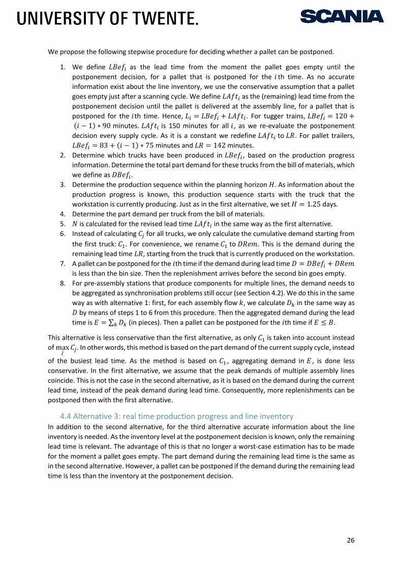
26
We propose the following stepwise procedure for deciding whether a pallet can be postponed.
1. We define 𝐿𝐵𝑒𝑓𝑖 as the lead time from the moment the pallet goes empty until the
postponement decision, for a pallet that is postponed for the 𝑖 th time. As no accurate
information exist about the line inventory, we use the conservative assumption that a pallet
goes empty just after a scanning cycle. We define 𝐿𝐴𝑓𝑡𝑖 as the (remaining) lead time from the
postponement decision until the pallet is delivered at the assembly line, for a pallet that is
postponed for the 𝑖th time. Hence, 𝐿𝑖 = 𝐿𝐵𝑒𝑓𝑖 + 𝐿𝐴𝑓𝑡𝑖 . For tugger trains, 𝐿𝐵𝑒𝑓𝑖 = 120 +
(𝑖 − 1) ∗ 90 minutes. 𝐿𝐴𝑓𝑡𝑖 is 150 minutes for all 𝑖 , as we re-evaluate the postponement
decision every supply cycle. As it is a constant we redefine 𝐿𝐴𝑓𝑡𝑖 to 𝐿𝑅. For pallet trailers,
𝐿𝐵𝑒𝑓𝑖 = 83 + (𝑖 − 1) ∗ 75 minutes and 𝐿𝑅 = 142 minutes.
2. Determine which trucks have been produced in 𝐿𝐵𝑒𝑓𝑖 , based on the production progress
information. Determine the total part demand for these trucks from the bill of materials, which
we define as 𝐷𝐵𝑒𝑓𝑖.
3. Determine the production sequence within the planning horizon 𝐻. As information about the
production progress is known, this production sequence starts with the truck that the
workstation is currently producing. Just as in the first alternative, we set 𝐻 = 1.25 days.
4. Determine the part demand per truck from the bill of materials.
5. 𝑁 is calculated for the revised lead time 𝐿𝐴𝑓𝑡𝑖 in the same way as the first alternative.
6. Instead of calculating 𝐶𝑗 for all trucks, we only calculate the cumulative demand starting from
the first truck: 𝐶1. For convenience, we rename 𝐶1 to 𝐷𝑅𝑒𝑚. This is the demand during the
remaining lead time 𝐿𝑅, starting from the truck that is currently produced on the workstation.
7. A pallet can be postponed for the 𝑖th time if the demand during lead time 𝐷 = 𝐷𝐵𝑒𝑓𝑖 + 𝐷𝑅𝑒𝑚
is less than the bin size. Then the replenishment arrives before the second bin goes empty.
8. For pre-assembly stations that produce components for multiple lines, the demand needs to
be aggregated as synchronisation problems still occur (see Section 4.2). We do this in the same
way as with alternative 1: first, for each assembly flow 𝑘, we calculate 𝐷𝑘 in the same way as
𝐷 by means of steps 1 to 6 from this procedure. Then the aggregated demand during the lead
time is 𝐸 = ∑ 𝐷𝑘𝑘 (in pieces). Then a pallet can be postponed for the 𝑖th time if 𝐸 ≤ 𝐵.
This alternative is less conservative than the first alternative, as only 𝐶1 is taken into account instead
of max𝑗
𝐶𝑗. In other words, this method is based on the part demand of the current supply cycle, instead
of the busiest lead time. As the method is based on 𝐶1 , aggregating demand in 𝐸 , is done less
conservative. In the first alternative, we assume that the peak demands of multiple assembly lines
coincide. This is not the case in the second alternative, as it is based on the demand during the current
lead time, instead of the peak demand during lead time. Consequently, more replenishments can be
postponed then with the first alternative.
4.4 Alternative 3: real time production progress and line inventory In addition to the second alternative, for the third alternative accurate information about the line
inventory is needed. As the inventory level at the postponement decision is known, only the remaining
lead time is relevant. The advantage of this is that no longer a worst-case estimation has to be made
for the moment a pallet goes empty. The part demand during the remaining lead time is the same as
in the second alternative. However, a pallet can be postponed if the demand during the remaining lead
time is less than the inventory at the postponement decision.

27
A detailed step-by-step procedure is:
1. As the line inventory is known, only the remaining lead time, LR is relevant. Hence, the lead
time starts at the postponement decision instead of the moment the pallet goes empty. This
means that 𝐿𝑅 is 150 and 142 minutes for tugger trains and pallet trailers respectively.
2. Determine the production sequence within the planning horizon 𝐻 = 1.25 days. As
information about the production progress is known, this production sequence starts with the
truck that the workstation is currently producing.
3. Determine the part demand per truck from the bill of materials.
4. 𝑁 is calculated for the revised lead time 𝐿𝐴𝑓𝑡𝑖 in the same way as the first alternative.
5. Just as in the second alternative, we only calculate the cumulative demand starting from the
first truck: 𝐷𝑅𝑒𝑚 = 𝐶1. This is the demand during the remaining lead time 𝐿𝑅, starting from
the truck that is currently produced on the workstation.
6. We define 𝐼𝑝𝑜𝑠𝑡 as the line inventory at the postponement decision moment. In most cases,
𝐼𝑝𝑜𝑠𝑡 is less than the bin size, as the first bin has already been empty for some time.
7. A pallet can be postponed for the 𝑖th time, if 𝐷𝑅𝑒𝑚 ≤ 𝐼𝑝𝑜𝑠𝑡. Then the replenishment arrives
before the second bin goes empty.
8. For pre-assembly stations that produce components for multiple lines, the demand needs to
be aggregated as synchronisation problems still occur (see Section 4.2). We aggregate demand
in the same way as in the second alternative. Then the aggregated demand during the
remaining lead time 𝐸 = ∑ 𝐷𝑅𝑒𝑚𝑘𝑘 (in pieces). A pallet can be postponed if 𝐸 ≤ 𝐼𝑝𝑜𝑠𝑡.
This alternative is less conservative than the second alternative, as it only makes an estimation of the
demand during the remaining lead time. The part of the lead time before the postponement decision
is disregarded as 𝐼𝑝𝑜𝑠𝑡 is known. For that reason, more pallets can be postponed with the third
alternative than with the second.
4.5 Comparison of alternatives The postponement of a pallet does not result into a line stoppage as long as the bin size is more than
the demand during the lead time of the pallet. The bin size is known, but the demand during lead time
is stochastic. We use a conservative perspective for predicting the lead time during lead time, such
that stock outs are prevented. The more information is available, the more accurately the demand
during lead time can be predicted. For that reason, more accurate information results in less
overestimation of the peak demand, which results into more pallets that can be postponed. In other
words, the alternative becomes less conservative if more information is available.
Alternative 1 requires the least information, but also the least number of pallets can be postponed.
The most pallets can be postponed for the third alternative, but this also requires the most accurate
information. The more pallets can be postponed, the more the workload can be levelled. However,
this comes with the price of obtaining and controlling information. For all alternatives, the bill of
materials, the planned production sequence and the bin size need to be known; this information is
readily available at Scania’s ERP-system. In addition to that, the second and third alternative require
real-time information about the production sequence. We suspect that obtaining this information does
not require large investments or organisational changes. For example, if the production progress of
one workstation is known, the production progress of the other workstation of that assembly line can
be deducted from that. Alternative 3 also requires information about the line inventory. We expect
that obtaining this information accurately is hard as only a little deviation from the actual inventory
could result in an incorrect postponement decision. Because nearly no deviations are allowed,

28
rejections of parts need to be correctly registered. Chapter 5 evaluates whether these additional
(information) requirements offset the potential of more accurate information.
Moreover, calculations for the first alternative can be done in advance, whereas calculations for
Alternatives 2 and 3 need to be done at the postponement decision. Alternative 1 only has to be
recalculated if the planned production sequence changes (for example during the night run of the ERP-
system). Therefore, Alternative 1 needs less computational effort/a less efficient algorithm than the
other two alternatives. Moreover, there is a risk of a delayed release of a replenishment request if
calculations of Alternatives 2 and 3 take too much time.
4.6 Levelling workload by postponing replenishments Sections 4.2, 4.3 and 4.4 have introduced methods for determining which pallets can be postponed.
This section proposes a method for determining which pallets are actually postponed and which pallets
are supplied immediately. A pallet is postponed one cycle at a time in order to base the postponement
decision on the most recent information. In other words, at the start of each supply cycle, we decide
whether a pallet is postponed an additional supply cycle.
The objective of postponing replenishments is to create a levelled workload that is beneficial to the
capacity utilisation. Only the peaks in workload are relevant, as these define the required capacity. In
other words, periods with higher workload result in higher capacity requirements, whereas periods
with lower workload result in idle capacity. For that reason, we propose a method in which pallets are
only postponed in periods of high workload. In short, our method postpones pallets if the workload is
above a certain threshold. The postponement is only based on the current supply cycle. A disadvantage
is that pallets can be postponed from busy periods to even busier periods. An alternative would be to
predict future workload and to base the postponement on this future workload. However, an accurate
prediction of when a pallet will empty is required to predict the future workload; the reasoning for not
advancing pallets has the same arguments (Section 4.1). Moreover, postponing pallets from busy
periods to busy periods does not result into a higher workload, as long as enough pallets can be
postponed in the latter period; we explain this by means of an example. Suppose that without
postponing, the workload in supply cycles 1, 2 and 3 is 10, 12 and 3 pallets. Suppose that we consider
9 pallets as a high workload. Then 1 pallet of cycle 1 is postponed to cycle 2. if no pallets can be
postponed in cycle 2, the resulting workload is worsened: 9, 13 and 3 pallets. However, this problem
does not occur if enough pallets can be postponed in the second cycle. In that case, 12+1-10 = 3 pallets
are postponed from cycle 2 to 3. The resulting workload is 9, 9 and 6 pallets.
We conclude that predicting the future workload is only beneficial if not enough pallets can be
postponed in each supply cycle. If enough pallets can be postponed, predicting the future workload
will make the method unnecessarily difficult. For that reason, we base the postponement of pallets
only on the current supply cycle; Chapter 5 evaluates the proposed method, from which we can
conclude whether enough pallets can be postponed for disregarding the prediction of workload.
To quantify high workload, we define, 𝑃𝑜𝑠𝐵𝑜𝑢𝑛𝑑, the postponement boundary, as a capacity level;
above this capacity level pallets are postponed (if possible). This section explains this in more detail.
The workload is ideally levelled if the workload in every cycle equals the average workload. If the
postponement boundary is set too high, no levelling takes place, as no or few pallets are postponed. If
the postponement boundary is set too low, the workload is not levelled but only shifted in time.
Before going into detail on the postponement process, we define two types of capacity:
• Regular capacity: planned capacity that is used to supply pallets to the assembly line.

29
• Extra capacity: unplanned capacity that is used to supply pallets to the assembly line, if the
pallets do not fit within the regular capacity. These trains are driven by troubleshooters or
team leaders that are called away from their regular activities.
Furthermore, we define two capacity levels. These levels only apply to the regular capacity, as we
assume that the extra capacity can be increased unrestrictedly.
• The maximum capacity: the physical capacity of a train or trailer, i.e. if the maximum capacity
is reached no more pallets fit on the train. Section 2.6 states that this capacity is 20 m3 for
pallet trailer supply zones and 9 EUR6-units for tugger trains.
• The postponement boundary (𝑃𝑜𝑠𝐵𝑜𝑢𝑛𝑑): capacity level above which pallets are postponed,
i.e. if the postponement boundary is reached, additional pallets are postponed if this is
possible.
Figure 23 illustrates the different capacity levels. The original workload is the workload in case no
postponements takes place. If possible, pallets are postponed as long as the workload is above the
postponement boundary. Extra capacity is used in case the supply of the remaining pallets that cannot
be postponed, does not fit within the maximum capacity. As extra capacity is unplanned, the usage of
this capacity should be reduced. For that reason, the postponement boundary is at most equal to the
maximum capacity level. Moreover, the postponement boundary has to be above the average
workload in order to create a stable postponement process. By setting the postponement boundary
below the maximum capacity level, the workload is further balanced. This is beneficial for the logistical
employees; they prefer a balanced workload above a process with periods of high and low workload.
In Chapter 5, we evaluate the proposed alternatives for different levels of 𝑃𝑜𝑠𝐵𝑜𝑢𝑛𝑑.
Figure 23: Explanatory graph of the defined capacity levels.
An advantage of the first alternative is that calculations can be done in advance, for example during
the night run of the ERP-system. The peak demand depends on 𝑖, the number of supply cycles a pallets
is postponed. Therefore, we need to calculate the peak demand for different values of 𝑖. We calculate
the peak demand for 𝑖 ∈ {1, 2, … , 𝑇𝑀𝑎𝑥}. This means that a pallet can be postponed at most 𝑇𝑀𝑎𝑥
times for Alternative 1. For the second and third alternative, the calculations cannot be done in
advance; therefore, no 𝑇𝑀𝑎𝑥 is required. However, we still restrict the postponement of pallets to
𝑇𝑀𝑎𝑥 times for Alternative 2 and 3, such that it a fair comparison with Alternative 1 can be made. We
expect that this restriction does not harm the performance of the proposed solution as long as it is not
set too tight. In Chapter 5, we evaluate the proposed alternatives for different levels of 𝑇𝑀𝑎𝑥.
0%
20%
40%
60%
80%
100%
120%
Cap
acit
y
Explanatory graph of capacity levels
Original workload Average Workload Maximum Capacity Postponement boundary

30
We distinguish between two categories of pallets:
A. Requests that cannot be postponed; this is based on the proposed methods in Sections 4.2,
4.3 and 4.4. Also, the number of times a pallet can be postponed is restricted.
B. Requests that can be postponed; this is based on the proposed methods in Sections 4.2, 4.3
and 4.4, as long as the restriction on the maximal number of postponements is not reached.
Figure 24 illustrates the different steps in deciding which pallets are immediately supplied and which
are postponed. These steps are taken at the start of each supply cycle. First, the available requests
(newly scanned requests and older postponed requests) are categorised. Requests of category A have
to be supplied to the assembly line as they cannot be postponed. Supply via regular capacity is
preferred as this capacity is planned, whereas the capacity of extra trains is unplanned capacity.
Therefore, requests of category A are assigned to the regular trains (step I.a), as long as the maximum
(physical) capacity is not reached. If the maximum capacity is reached, these requests are supplied by
means of extra capacity (step I.b). As requests of category B can be postponed we only supply them if
the postponement boundary is not reached (step II.a). Otherwise, the requests are postponed (step
II.b), such that the workload is levelled. As the postponement boundary is set below the maximum
capacity, requests of category B are not supplied by means of extra capacity. Actually, it could be
beneficial to supply these pallet if the extra capacity is already required for other pallets. However, for
sake of simplicity, we do not take into account this possibility. This is desired, as otherwise
unnecessarily capacity is (temporarily) increased. The current situation at Scania can be considered as
the situation in which only pallets of category A exist. This corresponds with step I of Figure 24.
Figure 24: Decision steps in the postponement process of requests. In the illustration a tugger train is used, but for a pallet trailer the same steps are made.

31
4.7 Conclusions We propose three alternatives for levelling the workload at Unit Supply Pallets. These alternatives take
into account the stochastic part demand at Scania. All three solution alternatives are based on
postponing pallets from periods with a high workload to periods with lower workload. The first
alternative is a conservative solution; it is conservative such that the lack of information about the
production progress and line inventory is overcome. The postponement of pallets is based on the peak
demand during lead time: the busiest lead time in the planning horizon. More pallets can be postponed,
if information about the production progress and line inventory is available. Information about the
production progress makes is possible to make a more accurate forecast of the part demand during
lead time. If information about the line inventory is available, more accurately can be determined
whether there is still enough remaining inventory for the demand during the remaining lead time. The
second alternative is based on the production progress information; the third alternative utilizes the
information of the production progress and the line inventory. By means of a more accurate prediction
of the demand during lead time, the second and third alternatives are less conservative, while ensuring
that no stock outs occur at the assembly line. For that reason, more pallets can be postponed, if more
information is available. However, obtaining this information requires investments and/or
organisational changes, as this information is not readily obtainable in the current situation; this is
especially true for accurate line inventory information.
Each supply cycle, it is determined which pallets are actually supplied and which are postponed. This
postponement decision is only based on information of the current supply cycle. Theoretically, this
could result in situations that pallets are postponed from periods with a high workload to periods with
an even higher workload. However, in practice this is not a problem as long as enough pallets can be
postponed. Which pallets are postponed is based on the postponement boundary. This means that if
the workload of a supply cycle is above a pre-defined threshold, pallets are postponed to the next
supply cycle as long as the pallet can be postponed. Chapter 5 investigates the performance of the
alternatives by means of a simulation study.

32

33
5. Simulation model This chapter investigates the postponement solutions proposed in Chapter 4 by means of a simulation
model. First, Section 5.1 describes important aspects for evaluating the proposed solution. Furthermore,
it gives an overview of the modelling steps and lists the main assumptions of the model. Section 5.2
describes the input of the model and Section 5.3 the output of the model. Section 5.4 addresses the
verification and validation of the model. Section 5.5 states the different scenarios investigated by the
simulation model. Section 5.6 gives the results of the simulation model. Finally, Section 5.7 draws
conclusions from the simulation study.
5.1 Model description We use a simulation model to investigate the consequences of implementing the postponement of
replenishments. Several aspects of the solution alternatives are important to evaluate the proposed
solutions. These aspects are described below and translated into KPIs in Section 5.3.
• Levelled workload: the main objective is a levelled workload at the part feeding process. To
be more precise: the supply of pallets should be balanced over the different supply cycles. As
the workload at part feeding is directly linked to the supply of pallets, the levelling of workload
can be achieved by levelling the supply of pallets. That is also the reason why we model the
supply of pallets as one process step, i.e. we aggregate the different sub-process steps of the
supply of pallets (such as transport by trains and changing pallets at the assembly line by
forklifts).
• Capacity utilisation: the reason behind levelling workload is that less capacity is needed for a
more balanced workload. The simulation model incorporates both the utilisation of the
regular capacity as well as the use of extra capacity.
• Stock outs: a stock out at the assembly line should be prevented, as it could result in a costly
line stoppage. The proposed alternatives of Chapter 4 are designed such that stock outs are
prevented. We do not explicitly model these stock outs in the simulation model, as they are
already incorporated in postponement decision, i.e. we only postpone pallets that cannot
result into costly line stoppage.
Modelling replenishment requests The core of the simulation model is the decision of which replenishments are supplied immediately
and which are postponed. Hence, these replenishment requests need to be generated by the model.
We state several alternatives for modelling these requests:
• The simplest solution is to directly use historical data of the requests as input of the model.
The main advantage of historical data is that interdependencies between requests are
incorporated in the historical data. Disadvantages are a lack of data and that only the historical
situation can be evaluated. This last disadvantage is the main reason why we do not directly
use historical data in our model.
• Requests can be generated by modelling the time between two consecutive requests of one
part. However, interdependencies between parts cannot be modelled via this alternative, e.g.
between the part demand of a left tail light and a right tail light. It does not incorporate the
difference in part demand between certain truck models. Assuming independence between
parts would underestimate peaks in requests. Therefore, we do not use this modelling method.
• A third way of modelling is deriving the part demand from the production sequence and bill of
materials. An advantage of this method is that the interdependencies between the part
demand for one truck are incorporated in the model. More processes such as the production
progress and the line inventory need to be modelled. However, these processes are also

34
required for modelling the postponement decision based on real time information (see Section
4.3). Section 5.2 describes in more detail how we model the input of our model.
Overview of the model This subsection describes the model briefly, before explaining the model more technically. The
simulation time series is divided in supply cycles. In each supply cycle the production progress is
updated and requests are created. At the initialisation of the model the production sequence is
generated by drawing trucks randomly from a historical set of trucks. Each supply cycle, the production
of trucks is simulated. For the trucks that are produced, the part demand is obtained via the bill of
materials. This part demand is deducted from the line inventory and requests are created for empty
pallets. The created requests are supplied or postponed according to the methods that Chapter 4
proposes.
Scania produces trucks on multiple assembly lines. We define the production flow 𝑎 as all the trucks
(or components of trucks) that are produced on the same assembly line 𝑎 . Workstations at the
assembly line produce for only one production flow 𝑎 , whereas pre-assembly workstations can
produce components for multiple production flows.
Section 5.2 explains the generation of the production sequence at the initialisation of the model. At
the start of each supply cycle, the model generates requests via the following modelling steps:
1. The demand during the lead time depends on the trucks that are produced in the previous
supply cycle (Figure 25). We define 𝑇𝑤,𝑎 as the number of trucks that have been produced in
the previous supply cycle for flow 𝑎 on (pre-assembly) workstation 𝑤. 𝑇𝑤,𝑎 is drawn from an
empirical distribution that Section 5.2 explains in more detail. In other words, 𝑇𝑤,𝑎 trucks have
been produced since the start of the previous supply cycle.
Figure 25: 𝑇𝑤,𝑎 is the number of produced trucks between the start of the previous supply cycle and the current
supply cycle.
2. We define 𝑉𝑝 as the demand for part 𝑝 in the previous supply cycle. Retrieve this part demand
for the 𝑇𝑤,𝑎 produced trucks from the production sequence and the bill of materials.
3. Update 𝐼𝑝, the line inventory of part 𝑝, by subtracting the part demand from the inventory
level at the start of the supply cycle.
4. Create replenishment requests for empty pallets, just as in the current situation.
5. For all replenishment requests, determine whether the replenishment is supplied immediately
or is postponed. This postponement decision is taken according to Sections 4.2, 4.3 and 4.4.
Appendix B contains a flowchart of the implementation of the postponement decision in the
simulation model. In the model, information about the production progress or line inventory
is known that is not available as defined in each alternative. The model only uses the
information as described in Chapter 4; additional information is not used at the postponement
decision in the model.
35
Model assumptions A simulation model is a simplification of reality; hence we list our important choices and assumptions:
• The actual supply of pallets is modelled as one process step with a deterministic process time.
This process time is equal to the lead time starting from the postponement decision moment
(see Figure 20 in Section 4.2).
• Only the supply of pallets is incorporated in the model; the return flow is left out of the
simulation model.
• The capacity of supplying pallets is restricted by the physical capacity of the tugger trains/
pallet trailers. Other restrictions, e.g. driving times, are not incorporated in the model.
• The part demand is fully defined by the need according to the bill of materials, e.g. the
rejection of parts is not taken into account.
• Rescheduling trucks is not incorporated in the simulation model.
• We do not change the current division of parts over the supply zones.
• The production process is modelled by means of generating 𝑇𝑤,𝑎 (see Section 5.2). Line
stoppages and other disruptions of the production process are implicitly incorporated in this
number of produced trucks. Moreover, stochastic cycle times are indirectly modelled via 𝑇𝑤,𝑎.
5.2 Input of the model The input of the model consists of three main components. First, a production sequence is generated
by means of a historical set of trucks. Second, an empirical distribution is used for generating 𝑇𝑤,𝑎. Last,
the bill of materials is used for retrieving the part demand of the trucks in the production sequence.
Production sequence A production sequence is generated for each workstation. This sequence is generated by randomly
drawing trucks from a historical set of trucks. This set of trucks is retrieved from the trucks that are
produced in February 2018. As the trucks are drawn randomly, there exists independence between
the trucks and therefore also between the workstations. In reality this is not the case as the production
planning process defines the production sequence (Section 2.3). For example, by using spacing
constraints dependencies in the production sequence is caused. As supply takes place in a cyclical way,
the part demand for trucks that are produced in the same supply cycle is aggregated. Hence, the impact
of the independence assumption is less. At Scania, pre-assembly stations produce for multiple
assembly lines. For these stations, a separate production sequence is generated for the production for
each assembly line.
Number of trucks produced per supply cycle We model the production progress by means of 𝑇𝑤,𝑎: the number of trucks that have been produced
on work station 𝑤 for flow 𝑎, 𝑇𝑤,𝑎 since the start of the previous supply cycle until the start of the
current supply cycle (see Figure 25). Each supply cycle, 𝑇𝑤,𝑎 is generated from an empirical distribution,
which is based on historical production data from February 2018. For this data set, we count the
number of produced trucks between two consecutive supply cycle starting times. These counted
frequencies are used as an empirical distribution. We choose for modelling production by means of
𝑇𝑤,𝑎 as it incorporates the stochastic behaviour of production, i.e. a high 𝑇𝑤,𝑎 correspond to a supply
cycle with few line stoppages and a lower 𝑇𝑤,𝑎 corresponds to more/longer line stoppages.
Bill of materials The bill of materials is used for determining the need of parts for each truck in the (generated)
production sequence. This bill of materials is readily available in Scania’s ERP-system and retrieved for
the trucks that are generated in the production sequence.

36
5.3 Output of the model We categorise the output of the simulation model in ‘levelled workload’ and ‘capacity utilisation’.
These measurements are created for each supply cycle. Aggregated measurements are calculated per
supply zone and per supply type (tugger train or pallet trailer), e.g. the mean and coefficient of
variation. For pallet trailers, we measure the supply size as the volume of the supplied pallets; for
tugger trains we measure the number of EUR6-positions needed (see Section 2.6).
Levelled workload Only the peaks are relevant for levelling the workload; during peaks in workload extra capacity is
needed, whereas in quiet periods (personnel) capacity cannot be reduced on short term. To able to
measure these peaks we introduce the concept of expected shortfall, which is commonly used in risk
management. The expected shortfall at 𝑞%-level is the expected loss of the worst 𝑞% cases (Hull, 2015)
of 𝑛 measurements. If 𝑛 ∗ 𝑞% is non-integer, ⌊𝑛 ∗ 𝑞%⌋ (rounding down) is used. In our situations, the
worst-case losses correspond with the cycles with the highest supply. Based on the expected shortfall
we define the expected peak at 𝑞%-level as the expected value of the 𝑞% highest peaks. The expected
peak is an indicator of the peaks in workload.
We illustrate the expected peak with an explanatory output in Figure 26, where we set 𝑞% = 20%.
The output contains 10 cycles, so the 20% highest peaks are those of cycle numbers 3 and 10 that have
respectively 9 and 8 requests. The average of these 20% highest peaks is 8.5. Hence, the expected peak
is 8.5 for a 20%-level. The main advantage of the expected peak is that not only the maximal peak is
taken into account, but that it is based on multiple peaks. Hence, the expected peak is less dependent
on a coincidence in the output than the maximal peak. For evaluating different scenarios, we use 𝑞%
= 20%. If 𝑞% is set too low, the expected peak approaches the maximal peak, which was the reason for
introducing the expected peak in the first place. If 𝑞% is chosen too high, the expected peak tends to
the average supply size, i.e. the height of peaks is underestimated as not only the peaks are included
into the expected peak.
Figure 26: Explanatory output for describing the expected peak with a q%-level of 20%. Here the expected peak is 8.5 (the mean of the third and tenth cycle).
Including this introduced indicator, the output for measuring levelled workload of our model is:
• Expected peak per supply cycle
• Average volume/EUR6-postions of requested replenishments.
• Average volume/EUR6-postions of postponed pallets.
• Average volume/EUR6-postions of pallets that are supplied to the line.
• Average volume/EUR6-positions of pallet that could have been postponed.
0
2
4
6
8
10
1 2 3 4 5 6 7 8 9 10
Cycle number
Number of requests

37
Capacity utilisation The objective of levelling the workload is that utilisation of capacity is improved. We distinguish
between regular capacity and extra capacity (see Section 4.6). Extra capacity is used in case more
pallets have to be supplied than fit in the maximum capacity of the pallet trailers or tugger trains. By
levelling the workload, the use of extra capacity is decreased. We expect that levelling the workload
does not directly improve the (average) utilisation of regular capacity, as the supply zones remain fixed
in the simulation model. Levelling the workload reduces the variation, whereas the average supply size
is not changed. The only change in the utilisation of the regular capacity is the shift of pallets from
extra to regular capacity. We still add the utilisation of the regular capacity to the output of the model
in order to make comparisons between supply zones. However, indirectly the utilisation of regular
capacity can be improved, by rebalancing the supply zones (see Chapter 6). Because of levelling the
workload, more pallets can be supplied by the same pallet trailer/ tugger train, while the probability
of having too little capacity remains the same.
The output of the model is:
• The utilisation of regular capacity, as calculated in Section 2.6.
• The proportion of supply cycles that need extra capacity for the supply of pallets.
• Average volume/EUR6-postions of pallets that are supplied by extra capacity.
5.4 Model verification and validation The simulation model is created in the 11th version of Plant Simulation. The model has been verified
according to the techniques proposed by Law and Kelton (1991) and Robinson (2004). The code has
been checked by running and debugging the code every few lines written. Visual checks of the pallet
flow through the model are performed by means of the animation function of Plant Simulation. Next
to that, we altered the input of the model to check whether it results in the expected outcome.
We validate the model by means of comparing the simulation model with observations of the real
system. We compare the requests generated by the simulation model with the replenishment requests
of the real system. The input for the model comparison is the planned production sequence and the
bill of materials of the trucks produced in February 2018. (Production days with more than three hours
of line stoppage are excluded.) The number of replenishments per supply cycle created by the model,
𝑋, is compared with the actual number of replenishments that have been scanned in each supply cycle,
𝑌. We cannot use a paired t-test, as the supply cycles in the simulation model cannot be paired with
the supply cycles in the real world. This is caused by differences in the production progress, i.e. the
production progress is simulated in the model and therefore not one-to-one comparable with the
production progress in the real system. However, we still expect that the distribution of 𝑋 and 𝑌 are
comparable. We use the chi-square goodness-of-fit test to test whether the observations of 𝑋 are from
the distribution of 𝑌 (Law and Kelton, 1991). Here we use the empirical distribution of 𝑌, based on the
trucks produced in February 2018. We select bin sizes such that each bin contains at least 5
observations and that the proportion of 𝑌 being in each bin is equal; this is called the equiprobable
approach. As 𝑌 is a discrete distribution the proportions of 𝑌 being in each bin is only approximately
equal. We performed this test for each supply zone (both pallet trailers and tugger trains); for all tests
the p-value is above 0.05. Therefore, we conclude that there is no statistical evidence that the
distribution of the number of requests per supply cycle in the simulation model deviates from the real
system. We refer to appendix C for more detailed results of the chi-square goodness-of-fit tests.
Next to comparison with the real system we use face validity: the simulation results are consistent with
the perceived system results (Law and Kelton, 1991). This face validation is performed by team leaders
of the part feeding process.

38
5.5 Experimental design
Scenarios By means of the simulation model, we evaluate the following four scenarios:
0. Current situation: this scenario is the current situation where no postponement takes place.
1. Peak demand: replenishments can be postponed if the peak demand of that request is less than
one pallet. Hence, pallets are postponed according to the first postponement alternative, as
described in Section 4.2.
2. Real-time production progress: a pallet can be postponed if the part demand during the lead time
is less than the bin size of the pallet. This scenario corresponds to the second postponement
alternative described in Section 4.3.
3. Real-time line inventory: a pallet can be postponed if the part demand during the remaining lead
time is less than the inventory level at the postponement decision. This scenario corresponds to
the third alternative in Section 4.4.
Parameters We perform sensitivity analyses for the following two parameters: 𝑃𝑜𝑠𝐵𝑜𝑢𝑛𝑑, the postponement
boundary and 𝑇𝑀𝑎𝑥, the maximal number of times a pallet can be postponed (for further explanation
of these parameters see Section 4.6). As these two alternatives have no effect on scenario 0, we
perform the sensitivity analyses only for each of the other three scenarios. For 𝑇𝑀𝑎𝑥, we evaluate
postponing pallets for at most 1, 2, 3, 4 or 5 times. (For tugger trains, postponing a pallet 5 times is
approximately equal to postponing an entire production shift.)
Let �̅� the average workload (measured in m3 or in EUR6-positions) and 𝑠 the sample standard deviation
of the workload, both obtained from the results of scenario 0. Section 4.6 states that the 𝑃𝑜𝑠𝐵𝑜𝑢𝑛𝑑
has to be above the average workload in order to create a stable postponement process. For that
reason, 𝑃𝑜𝑠𝐵𝑜𝑢𝑛𝑑 > �̅�. Setting 𝑃𝑜𝑠𝐵𝑜𝑢𝑛𝑑 depends on the standard deviation of the workload; the
lower the variation, the closer 𝑃𝑜𝑠𝐵𝑜𝑢𝑛𝑑 has to be to �̅� for levelling the workload. Hence, we
calculate 𝑃𝑜𝑠𝐵𝑜𝑢𝑛𝑑 = �̅� + 𝑘 ∗ 𝑠, for a certain level of 𝑘, 𝑘 > 0. For the sensitivity analyses, we use
𝑘 ∈ {0.25; 0.50; 0.75; 1,00; 1,25}.
For comparing the scenarios with each other, we select the middle of the values mentioned above; we
compare the scenarios for 𝑇𝑀𝑎𝑥 = 3 and 𝑘 = 0.75.
Warm-up period The simulated system is a non-terminating system, as production is stopped at the end of the day but
continued at the start of the day. We are interested in the steady-state cycle performance, where the
cycles are the supply cycles. The warm-up period is determined by means of Welch’s graphical
procedure (Law and Kelton, 1991). The warm-up period is based on the number of pallets supplied per
supply cycle, for 𝛾 = 0.05 and based on the first scenario. We choose this scenario, as it has the highest
variation in supply; by postponing pallets the supply of pallets is levelled. This procedure is repeated
for each supply zone. Appendix D shows the results for all supply zones. The warm-up period is set
equal to the longest warm-up period of 7 supply cycles is found for tugger train 1C.
Run length and number of replications We use the replication/deletion approach (Law and Kelton, 1991) for obtaining the performances of
the simulation model. This means that for each replication the model is initialized and that each
replication has its own warm-up length. An alternative is to perform one long run (with one warm-up
length) that includes all replications; this is called the batch means approach. Despite a longer running
time, we choose for the replication/deletion approach. The main advantage of the replication/deletion

39
approach is that correlation between replications is eliminated. We set the run length much longer
than the warm-up period, such that any remaining initialisation bias is removed from the performance
output; the run length is 40 supply cycles.
We use the sequential procedure introduced by Law and Kelton (1991) for determining the number of
replications required, such that a confidence level of 95% is obtained. Just as for the warm-up period,
the number of replications is based on the number of pallets supplied per supply cycle and determined
for each supply zone. The number of replications differs from 4 to 12 replications. Therefore, we set
the number of replications equal to 12; this number of replications is found for Tugger train 1A.
5.6 Results of simulation study This section gives the results of the simulation model. First, this section evaluates the scenarios based
on how much the workload is levelled. After that, it evaluates the capacity utilisation of the different
scenarios. Furthermore, sensitivity analyses are performed on the postponement boundary
(parameter 𝑘) and the maximal number of times a replenishment can be postponed (𝑇𝑀𝑎𝑥). Appendix
E explains several statistical techniques that are used in the analysis of the results. Appendix F contains
the 95%-confidence intervals of the output of the simulation model.
Levelled workload The main objective of our proposed adaptations (Sections 4.2, 4.3 and 4.4) of the Unit Supply Pallets
process, is the levelling of workload. We use the expected peak defined in Section 5.3 to determine
how much the workload is levelled. Figure 27 shows the expected peak for pallet trailers and Figure 28
for tugger trains, both for 𝑇𝑀𝑎𝑥 = 3 and 𝑘 = 0.75. This expected peak is the average workload for
the 20% busiest supply cycles. To recall, Scenario 1 utilizes the least information and Scenario 3 the
most.
For pallet trailers, postponing pallets results in lower peaks. Compared with the current situation,
Scenario 1 reduces the peak on average with 6.8%, Scenario 2 with 10.8% and Scenario 3 with 12.2%
(Figure 27). In absolute terms, the expected peaks are reduced with respectively 0.81, 1.22 and 1.39
cubic metres. For all supply zones, these differences are significant, based on paired t-95%-confidence
intervals. We conclude that the more information is available, the lower the expected peak. Based on
these reductions, we conclude that postponing pallets is beneficial to levelling the workload. For
Scenario 2, information about the production progress is required; this required information is paid off
by an extra reduction of workload peaks of 4 percent points compared with Scenario 1. Scenario 3
results only in a slightly bigger reduction (1.4 percent points) of the workload than Scenario 2, although
accurate information about the line inventory is needed, which is hard to obtain. Therefore, we
conclude that obtaining the accurate information of the line inventory is not paid off by a reduction in
workload.
Figure 28 shows a remarkable pattern for most tugger train zones: postponing pallets levels the
workload, but no noticeable differences occur between Scenarios 1, 2 and 3. The average reduction is
bigger for tugger trains than for pallet trailers: Scenario 1 reduces the peak on average with 26.2%,
Scenario 2 with 27.9% and Scenario 3 with 29.9%. In absolute terms, the expected peaks are reduced
with respectively 1.59, 1.71 and 1.86 EUR6-positions. This is according to our expectations, as the
tugger trains zones supply less pallets than the pallet trailer zones (see Section 2.5). Hence, in the
current situation more variation occurs at tugger trains than at pallet trailers, as explained by the law
of large numbers. For most tugger train zones, the differences between Scenarios 1, 2 and 3 are
statistically insignificant; for some zones the differences are statistically significant, but as these
differences are small, we conclude that these (significant) differences are not relevant in practice. For

40
that reason, we conclude that extra information about the production progress and/or line inventory,
does not result into a more levelled workload for tugger trains.
Figure 27: Expected peak of the supply by means of pallet trailers. This expected peak is denoted in cubic metres. Scenarios are simulated for 𝑇𝑀𝑎𝑥 = 3 and 𝑘=0.75.
Figure 28: Expected peak of the supply by means of tugger trains. The expected peak is denoted in EUR6-positions. Scenarios are simulated for 𝑇𝑀𝑎𝑥 = 3 and 𝑘=0.75.
As concluded above, additional information about the production progress results into a more levelled
workload for pallet trailers, but not for tugger trains, i.e. Scenario 2 outperforms Scenario 1 for pallet
trailers, but not for tugger trains. An explanation for this is that for tugger trains already enough pallets
can be postponed for Scenario 1. Even though more pallets could be postponed with Scenario 2 (and
Scenario 3), this does not result in lower expected peaks as no more pallets are actually postponed
(these pallets are not postponed as the postponement boundary is not yet reached). This explanation
0
5
10
15
20
25
1A 1B 1C 2A 2B 2C 3A 3B 3C
Exp
ecte
d p
eak
(m3
)
Pallet trailer zone
Expected peak - pallet trailers
Scenario 0
Scenario 1
Scenario 2
Scenario 3
0
1
2
3
4
5
6
7
8
9
10
1A 1B 1C 2A 2B 2C 3A 3B 3C
Exp
ecte
d p
eak
(EU
R6
-po
siti
on
s)
Tugger train zone
Expected peak - tugger trains
Scenario 0
Scenario 1
Scenario 2
Scenario 3

41
is supported by Figure 29: The average per supply cycle of EUR6-positions of tugger train pallets that
are postponed and that could be postponed. Figure 29 and Figure 30 show the percentage of the
supplied pallets that could have been postponed and that actually have been postponed. As mentioned,
postponing pallets based on real-time production progress information results into lower peaks than
by postponing pallets based on peak demand, because more pallets can be postponed in Scenario 2
(and 3) than in Scenario 1.
Figure 29: The average per supply cycle of EUR6-positions of tugger train pallets that are postponed and that could be postponed. Scenarios are simulated for 𝑇𝑀𝑎𝑥 = 3 and 𝑘=0.75.
Figure 30: The average pallet volume (m3) of pallet trailer pallets that are postponed and that could be postponed per supply cycle. Scenarios are simulated for 𝑇𝑀𝑎𝑥 = 3 and 𝑘=0.75.
Capacity utilisation The aim of levelling the workload is to improve the utilisation of capacity. Here, we distinguish between
the utilisation of regular and extra capacity as defined in Section 5.3. Extra capacity is needed in case
more pallets need to be supplied than fit in the pallet trailers/tugger trains.
Figure 31 shows that the utilisation of the regular capacity of pallet trailers and tugger trains barely
changes when postponing pallets. This is according to our expectations, as levelling the workload does
0%10%20%30%40%50%60%70%80%90%
100%
Sce
n. 1
Sce
n. 2
Sce
n. 3
Sce
n. 1
Sce
n. 2
Sce
n. 3
Sce
n. 1
Sce
n. 2
Sce
n. 3
Sce
n. 1
Sce
n. 2
Sce
n. 3
Sce
n. 1
Sce
n. 2
Sce
n. 3
Sce
n. 1
Sce
n. 2
Sce
n. 3
Sce
n. 1
Sce
n. 2
Sce
n. 3
Sce
n. 1
Sce
n. 2
Sce
n. 3
Sce
n. 1
Sce
n. 2
Sce
n. 3
1A 1B 1C 2A 2B 2C 3A 3B 3C
Postponement of tugger train pallets per supply cycle
% of supplied EUR6-positions that are postponed % of supplied EUR6-positions that could be postponed
0%10%20%30%40%50%60%70%80%90%
100%
Sce
n. 1
Sce
n. 2
Sce
n. 3
Sce
n. 1
Sce
n. 2
Sce
n. 3
Sce
n. 1
Sce
n. 2
Sce
n. 3
Sce
n. 1
Sce
n. 2
Sce
n. 3
Sce
n. 1
Sce
n. 2
Sce
n. 3
Sce
n. 1
Sce
n. 2
Sce
n. 3
Sce
n. 1
Sce
n. 2
Sce
n. 3
Sce
n. 1
Sce
n. 2
Sce
n. 3
Sce
n. 1
Sce
n. 2
Sce
n. 3
1A 1B 1C 2A 2B 2C 3A 3B 3C
Postponement of pallet trailer pallets per supply cycle
% of supplied pallet volume that is postponed % of supplied pallet volume that could be postponed

42
not directly improve capacity utilisation as the average workload does not change. Regular capacity
utilisation can only be improved if locations are reallocated to supply zones. For some supply zones,
there seems to be a small difference between Scenario 0 and the other scenarios; this is caused by
supplying less/more pallet by means of extra capacity.
Figure 31: Capacity utilisation of the regular capacity of pallet trailers (left graph) and tugger trains (right graph) for 𝑇𝑀𝑎𝑥 =3 and 𝑘=0.75.
Figure 32: The proportion of supply cycles in which extra capacity is needed, determined for 𝑇𝑀𝑎𝑥 = 3 and 𝑘=0.75. Supply zones that are excluded from this figure do not need extra capacity. (TT = tugger train and PT = pallet trailer.)
For each supply zone, Figure 32 shows the proportion of supply cycles that need extra capacity for the
supply of pallets. Not all supply zones require extra capacity, because of their low utilisation (Figure
31); these supply zones are excluded from Figure 32. Postponing pallets (Scenarios 1, 2 and 3) results
in a lower need for extra capacity. Only for supply zones PT 1B, PT 1C, PT 2A, TT 1A, TT 2B, TT 2C and
TT 3B this reduction is statistical significant. In the current situation (Scenario 0), 3.63 times a day extra
capacity is needed for all supply zones in total (a pallet trailer zone is replenished 11.33 times a day
and a tugger train zone 9.67 times.) If pallets are postponed, this is 1.14, 0.33 and 0.12 times a day for
Scenario 1, 2 and 3 respectively. For a team leader or troubleshooter, it takes 30-45 minutes for
supplying pallets to the assembly by means of an extra train. Also, the regular activities of the team
0%
10%
20%
30%
40%
50%
60%
70%
80%
1A 1B 1C 2A 2B 2C 3A 3B 3C
Capacity utilisation - Pallet trailers
Scenario 0 Scenario 1 Scenario 2 Scenario 3
00%
10%
20%
30%
40%
50%
60%
70%
80%
1A 1B 1C 2A 2B 2C 3A 3B 3C
Capacity utilisation - Tugger trains
Scenario 0 Scenario 1 Scenario 2 Scenario 3
0,00%
1,00%
2,00%
3,00%
4,00%
5,00%
6,00%
7,00%
8,00%
9,00%
10,00%
PT 1B PT 1C PT 2A PT 3A TT 1A TT 1B TT 1C TT 2B TT 2C TT 3B
Percentage of supply cycles for which extra capacity is needed
Scenario 0 Scenario 1 Scenario 2 Scenario 3

43
leader are interrupted in case extra capacity is needed. By postponing pallets, from 92 minutes (=(3.63-
1.14)*37) to 130 minutes (=(3.63-0.12)*37) of supplying pallets by means of extra capacity can be
saved per day. From Figure 32, we conclude that if information about the production progress and line
inventory is available, a higher reduction of the extra capacity can be achieved.
Sensitivity analyses We compare the four scenarios for 𝑇𝑀𝑎𝑥 = 3 and 𝑘 = 0.75 . This subsection investigates the
sensitivity of the solution performance for these two parameters. We investigate the sensitivity of the
parameters on the main output of the model: the expected peak. As said in Section 4.6, if the
postponement boundary is set too high, no or only little levelling of the workload takes place. However,
if the postponement boundary is set too tight, the workload is only shifted in time instead of levelling
it. We do not take into account Scenario 0, because no pallets are postponed in that scenario.
Figure 33 and Figure 34 show that the longer a pallet may be postponed, the more balanced the
workload is. However, this is a diminishing effect; for 𝑇𝑀𝑎𝑥 ≥ 3, increasing 𝑇𝑀𝑎𝑥 any further does
not result into a more balanced workload. For tugger trains, the workload is levelled the most, when
𝑘 is set around 0.50 - 0.75. If 𝑘 is set lower then that, the expected peak increases, as too many pallets
are postponed; then the workload is shifted instead of balanced. If 𝑘 is set higher than that, the full
potential of postponing pallets is not achieved. The postponement boundary of pallet trains can be set
tighter than that of tugger trains; the most levelled workload is achieved with 𝑘 around 0.25 – 0.50.
In our opinion, it is better to set the postponement boundary somewhat too loose, than too tight. If it
is set somewhat too loose, an increase in part demand can be handled, whereas if the postponement
boundary is set too tight, an increase in part demand enlarges the problem of a too tight postponement
boundary. From the figures, we conclude that the problem of a too tight postponement boundary is
increased for low values of 𝑇𝑀𝑎𝑥. Therefore, we advise to set 𝑇𝑀𝑎𝑥 at least equal to 3 supply cycles
and 𝑘 somewhere around 0.50.
Figure 33: Effect of 𝑇𝑀𝑎𝑥 and 𝑘 on the expected peak for tugger trains. The average is taken over all supply zones.
0
1
2
3
4
5
6
0.25 0.5 0.75 1 1.25 0.25 0.5 0.75 1 1.25 0.25 0.5 0.75 1 1.25
Scenario 1 Scenario 2 Scenario 3
Avg
. exp
ecte
d p
eak
per
su
pp
ly z
on
e(E
UR
6-p
osi
tio
ns)
k
Expected peak - tugger trains
Tmax = 1 Tmax = 2 Tmax = 3 Tmax = 4 Tmax = 5

44
Figure 34: Effect of TMax and k on the expected peak for tugger trains. The average is taken over all supply zones.
5.7 Conclusions By means of a simulation study, we evaluate the three alternative solutions for levelling workload by
postponing replenishments as proposed in Chapter 4. The simulation model generates a production
sequence. For each supply cycle, the part demand is derived from the bill of materials and the
production sequence. Requests are made for pallets that go empty. These requests are processed
according to four scenarios:
• Scenario 0: the current situation in which no pallets are postponed.
• Scenario 1: pallets are postponed based on the peak demand during lead time.
• Scenario 2: pallets are postponed based on the demand during the lead time, that is obtained
from real-time information about the production progress.
• Scenario 3: pallets are postponed based on the demand during the remaining lead time, that
is obtained from real-time information about the production progress and line inventory.
We evaluate the four scenarios based on the aspects ‘levelled workload’ and ‘capacity utilisation’. The
expected peak size is an indicator for the height of the peaks and therefore also for how much the
workload is levelled. Table 3 summarises the performance of the different postponement alternatives
in comparison with the current situation.
Table 3: Performance output of different postponement alternatives compared with the current situation. Calculated for k=0.75 and TMax=3.
Scenario
Reduction of expected peak Reduction of extra capacity needed
Tugger trains (EUR6-positions)
Pallet trailers (m3)
Number of times per day
Hours per day
Scenario 1 1.59 (26.2%) 0.81 (6.8%) 2.49 (69%) 1.53 (69%)
Scenario 2 1.71 (27.9%) 1.22 (10.8%) 3.30 (91%) 2.03 (91%)
Scenario 3 1.86 (29.9%) 1.39 (12.2%) 3.51 (97%) 2.16 (97%)
The result of postponing pallets on levelling the workload is different for tugger trains and pallet
trailers. The percentage reduction of the expected peak (the average workload in the 20% busiest
cycles) is the highest for tugger trains. For tugger trains, no effect is noticeable on the expected peak,
if more accurate information is available. For pallet trailers this is only noticeable for using accurate
information about the production progress. The difference between pallet trailers and tugger trains
exists because more pallets can be postponed for the tugger trains than for the pallet trailers.
9
9,5
10
10,5
11
11,5
12
0.25 0.5 0.75 1 1.25 0.25 0.5 0.75 1 1.25 0.25 0.5 0.75 1 1.25
Scenario 1 Scenario 2 Scenario 3
Avg
. exp
ecte
d p
eak
per
su
pp
ly z
on
e (m
3)
k
Expected peak - pallet trailers
Tmax = 1 Tmax = 2 Tmax = 3 Tmax = 4 Tmax = 5

45
Postponing pallets has no effect on the utilisation of the regular capacity. However, the need for extra
capacity is reduced by at least 69% by means of postponing pallets (Table 3); the more accurate
information available the less extra capacity is needed. This reduction saves the team leaders about
1.5 hours per day that they need to support the supply of pallets. Moreover, they are called away from
their regular activities if they have to support with the supply of pallets.
Abovementioned evaluation is based on 𝑇𝑀𝑎𝑥 = 3 and 𝑘 = 0.75. We performed a sensitivity analysis
on these parameters. The higher 𝑇𝑀𝑎𝑥, the maximal number of times a pallet may be postponed, the
better the performance. However, for 𝑇𝑀𝑎𝑥 ≥ 3, the effect on the workload levelling diminishes. The
parameter 𝑘 sets the postponement boundary ( 𝑃𝑜𝑠𝐵𝑜𝑢𝑛𝑑 = �̅� + 𝑘 ∗ 𝑠 ). If the postponement
boundary is set too tight, no levelling of workload takes place but only shifting the peaks in time. Based
on the sensitivity analysis, we advise to set 𝑘 around 0.5 and 𝑇𝑀𝑎𝑥 at least equal to 3.
Based on the results of the simulation study, we conclude that by postponing pallets the workload is
balanced. Workload peaks are reduced, which is directly noticeable as the need for extra capacity is
greatly reduced. The three proposed postponement alternatives require different levels of information.
Scenario 2 requires additional information about the production progress and Scenario 3 about the
production progress and line inventory. From the simulation results, we conclude that is does not pay
off to obtain accurate information of the line inventory. This is hard to achieve and does not result in
lower workload peaks. Therefore, we advise to implement either Alternative 1 or 2. For levelling the
peak at tugger trains, information about the production progress does not result into additional
benefits. However, for pallet trailers information about the production progress (Scenario 2) results
into an extra reduction of the workload peaks and less extra capacity is needed. This information is not
readily available at Scania, but we suspect that obtaining this information does not require large
investments or organisational changes. Scenario 1 has the advantage that no real-time calculations are
needed. This advantage is mainly applicable in case it is hard to implement the calculations within the
current ERP-system.

46

47
6. Rebalancing supply zones This chapter proposes two Mixed Integer Programming models for rebalancing the supply zones of Unit
Supply Pallets for improving the capacity utilisation of Unit Supply Pallets. Section 6.1 explains the
reasoning for rebalancing supply zones. Section 6.2 describes alternatives for rebalancing the supply
zones. For rebalancing the supply zones, we propose a MIP-model that Section 6.3 explains. This MIP-
model allocates clusters of locations to tugger trains and pallet trailers. To reduce the problem size, this
problem is split into two subproblems that Sections 6.4 and 6.5 describe. Section 6.6 gives the results
from the MIP-models. Finally, Section 6.7 makes concluding remarks on rebalancing supply zones.
6.1 Why rebalancing supply zones? Rebalancing supply zones is the second step in improving the capacity utilisation by levelling the
workload. As Chapter 5 concludes, postponing pallets levels the workload, but does not directly
influence the utilisation of regular capacity. However, by reducing the variation, more pallets can be
supplied to the assembly line within one tugger train or pallet trailer, while keeping the need for extra
capacity constant. Figure 35 illustrates this with an example for a tugger train: suppose that without
postponing pallets the coefficient of variation of the supply equals 0.50. Extra capacity is needed in
case the supply is above the capacity of the tugger train. An average supply of at most 6 EUR6-positions
(orange line) is possible if the needed extra capacity is restricted to 2.5% of the supply cycles. If the CV
is reduced to 0.20, the average supply can be increased to 6.5 EUR6-positions, while keeping the
needed for extra capacity constant at 2.5% of the supply cycles. Summarizing, by postponing pallets,
the average supply can be increased while keeping the need for extra capacity constant. As tugger
trains and pallet trailers can supply more, more parts can be allocated to a certain supply zone. By
reallocating the parts to the supply zones, the utilisation of the regular capacity is improved.
Figure 35: By reducing the variation, the average supply can be increased (green arrows), while keeping the need for extra capacity constant. Here, the probability for needing extra capacity is 2.5%.
Moreover, the supply zones should be rebalanced if imbalances between supply zones occur, i.e. if the
capacity utilisation of one supply zone deviates much from that of another supply zone. Section 2.6
shows that some supply zones supply much more than other supply zones with the same capacity. By
reallocating parts to the supply zones, the differences in workload between the supply zones are
reduced.

48
6.2 Alternatives for rebalancing supply zones Rebalancing the supply zones means that part locations are (re)allocated to the pallet trailers and
tugger trains. Several alternative methods can be used for this allocation:
• Manually: the locations can be allocated manually to the supplying pallet trailers and tugger
trains. This manual allocation can be based on calculation performed in spreadsheets. The
main advantage of this method is that considerations that are hard to model can be
incorporated in the allocation as it is created by hand. Main disadvantages are that it is
unknown how good the allocation is and that for large-sized or heavily restricted problems it
can be hard to determine a feasible solution. Moreover, it is time-consuming to construct and
evaluate different proposed solutions. Therefore, mostly only a few (somewhat arbitrary)
allocation proposals are evaluated.
• Computer-aided decision making: the allocation of locations is done manually, but the
evaluation of proposed allocation is done by a computer program. In other words, after a
person has filled in an allocation, the program checks its feasibility and shows information
about the performance of the proposed allocation. The advantage of this alternative is that it
is easier to evaluate multiple allocations, while having full flexibility in considerations for the
allocation. However, no structured approach exists for finding a good or the best allocation.
Moreover, if the solution space is heavily restricted, it can be hard to find a feasible solution
(allocations are easily evaluated, but determining an allocation is not supported).
• Mixed Integer (Linear) Programming, MI(L)P: a mathematical optimisation technique that
describes the problem in terms of linear relationships. The main advantage is that the entire
solution space is evaluated, i.e. the found allocation is the optimal solution (or if calculation
time is restricted, it is known how far it is away from the theoretical optimum). The main
disadvantage of a MIP-model is that it cannot be solved if the solution space becomes too large,
also known as the curse of dimensionality. Furthermore, all restrictions of the allocation have
to be modelled as linear relationships.
• Optimisation heuristics: heuristics try to find good solutions, but not necessarily optimal
solutions, in a structural way. A main advantage is that many solutions can be evaluated
systematically, even if the solution space is large. A disadvantage is that it is unknown how far
away the solution is from the optimal solution. This disadvantage can be overcome if bounds
of the optimal solution can be determined. This means that by using characteristics of the
(optimal) solution, a bound states that the optimal solution value cannot be better than the
imposed bound.
We choose to construct the allocation by means of Mixed Integer (Linear) Programming, as it
investigates the (theoretical) optimal solution. This is valuable information, as it quantifies the full
potential of levelling the workload. For the other three alternatives, the full potential cannot be
quantified as the current situation can only be compared with the best solution found; however, it
could be that better solutions are possible that have not been found yet. This chapter proposes several
steps to reduce the size of the problem.
6.3 MIP-model description This section first describes the objective of the proposed model. After that it briefly describes the
model and which restrictions of the allocation problem are incorporated in the model. The model is
split into two subproblems; Sections 6.4 and 6.5 describes these two parts in more detail.

49
Objective of the model As stated in Section 6.1, the objective of rebalancing the supply zones is to improve the utilisation of
the (regular) capacity. This means that the required capacity should be minimized. However, it is hard
to compare a tugger train with a pallet trailer, as not only capacity utilisation is important, but also
factors as the effect on safety inside the plant. Therefore, the objective of our proposed model is not
to minimize the (number of) pallet trailers and/or tugger trains, but it optimises the capacity utilisation
given 𝑅 pallet trailers and 𝑇 tugger trains. Optimized means that the capacity utilisation is spread
evenly over the supply zones. Two alternatives for spreading the capacity utilisation are: 1. Minimizing
the maximal capacity utilisation or 2. Minimizing the total of the absolute differences between the
capacity utilisations and the mean capacity utilisation. Figure 36 illustrates these two measurement
methods. The figure shows the maximum capacity as the yellow and blue line. The maximal capacity
utilisation is relevant as the zone with the highest capacity utilisation is the busiest supply zone. The
red arrows in the figure indicate the absolute differences and as a measurement of the spread of the
capacity utilisation the sum is taken over these differences between the capacity utilisation and the
average capacity utilisation. This sum of the absolute differences is a linearization of the variation in
the capacity utilisation. We use the second alternative, because it incorporates the capacity utilisation
of all zones in the objective. This is not the case for minimizing the maximal capacity utilisation. There,
only the supply zone with the highest capacity utilisation is considered; if the busiest zone cannot be
lowered, the other supply zones are not optimised any further, as it does not influence the objective
value.
Figure 36: Example output for illustrating different measurements of spreading the capacity utilisation. PT = pallet trailer supply zone and TT = tugger train supply zone.
Broad description of the model The inventory locations at the assembly line and the pre-assembly stations are clustered in small
groups of locations that are near to each other. By clustering these locations, the problem size reduces.
Moreover, for the train drivers, it is undesired that locations that are next to each other are supplied
by different trains/trailers, because it is less clear which locations belong to which trains. The MIP-
model allocates each cluster of locations to a certain tugger train or pallet trailer supply zone. To recall,
tugger trains and pallet trailers supply three supply zones within a cycle of 90 or 75 minutes
respectively (Section 2.2). A supplying pallet trailer is disconnected near the assembly line at

50
predefined spots; forklifts change empty pallets with full pallets from the pallet trailer. A tugger train
drives along the locations and changes the empty pallets with full pallets itself. This model only takes
into account the supply flow and not the return flow.
The following restrictions apply to the allocation of clusters:
• Each tugger train and pallet trailer supply zone has a maximum (physical) capacity as defined
in Section 4.6, measured in EUR6-positions and cubic metres respectively.
• Certain location clusters cannot be supplied by tugger trains as they contain pallet racks, which
can only be supplied by forklifts, or they cannot be reached by pallet trains because of too
narrow alleys or too tight turns.
• A location cluster can only be allocated to a subset of pallet trailer zones; only those pallet
trailer zones that have disconnecting spots nearby. This restriction is added such that the
driving times of the forklift drivers are not too long. By interviewing team leaders and
operators, we determine for each location cluster by which pallet trailer zones it can be
supplied. Certain location clusters cannot be supplied by any pallet trailer zone as there is no
disconnecting spot nearby.
• A tugger train has got 30 minutes for supplying one supply zone. This time contains loading full
pallets at the warehouse, the driving time, the time of changing full pallets with empty pallets
at the assembly line, the scanning time of empty pallets, and the time for unloading empty
pallets at the pallet breakdown. Furthermore, still some time should be left within the
schedule to absorb process deviations. At Scania, 20% of the supply time is reserved for this;
this equals 6 minutes for tugger trains.
• The above-mentioned driving time of the tugger train depends on the locations it visits. Also,
a tugger train scans empty pallets of a supply zone that it delivers in the ride after the next
one. This also has to be incorporated in the tugger train route.
• The times within the process of the pallet trailer do not depend on how full they are loaded.
Also, the driving time of a pallet trailer is constant as the disconnecting spot is predefined.
Therefore, driving time of pallet trailers imposes no restrictions on the allocation of location
clusters and is left out of the MIP-model.
From these restrictions, we distinguish the subproblem of determining the shortest route of a tugger
train for supplying and scanning all its allocated locations. If the allocation of location clusters and the
determination of the shortest tugger train routes are done simultaneously, the problem instance
becomes too large to be solved by CPLEX (software for solving MIP-problems). Therefore, we split our
original problem into the following subproblems:
1. What is the shortest route of a tugger train, given the locations it has to visit.
2. How should the location clusters be allocated to the tugger trains and pallet trailers such that
the capacity utilisation is evenly spread, given the routes of the tugger trains.
To solve the problem, we first generate tugger train routes. Given the generated routes the allocation
problem is solved. This method results in the optimal allocation, given the generated routes. In our
method, all feasible routes are created, therefore, the allocation found will be the optimal allocation.
Section 6.4 explains the generation of routes and determining the shortest route length in more detail.
Section 6.5 describes the MIP-model used for the allocation problem, given the generated routes. This
splitting of the problem is based on column generation. Column generation is designed for LP problems
that have many variables but only a few constraints (Manthey, 2017). Instead of considering all
possible variables, it generates the variables that seem to improve the solution. Using column
generation for ILP problems is not possible if certain variables are not needed in the (relaxed) non-

51
integer solution, but that are required in the optimal integer solution. This is the reason why column
generation is not suitable for our problem. However, we use the method of generating variables
(tugger train routes) and then solving the remaining part of the problem.
6.4 Model description – Generating tugger train tours This section describes the generation of tugger train routes that are the input of the MIP-model for
allocating locations to the tugger trains and pallet trailers. The aim of generating routes is to determine
the driving times of all feasible routes, while filtering out as many routes that are infeasible in the
allocation problem. Determining the (shortest) driving times of the routes is required as each tugger
train has a limited time for supplying pallets in a supply cycle. By filtering out infeasible routes, the
calculation time for solving the allocation problem decreases.
The tugger train routes are generated such that the driving time is known for all feasible routes of the
tugger trains. Given these generated routes, a second MIP-model allocates the locations clusters to
pallet trailer and tugger train zones (Section 6.5). Generating routes is done in four steps (Figure 37).
First, all possible combinations of location clusters in a route are generated. Second, the combinations
that violate the capacity of the tugger train, are filtered out that. In the third step, for each of the
remaining routes, a MIP-model determines the shortest driving time for visiting all location clusters. In
the fourth step, all routes are filtered out that have a too long driving time. The remaining routes are
the input of the second MIP-model, which Section 6.5 describes. The remainder of this section explains
the four steps in more detail.
Figure 37: Overview of the four steps for generating the tugger train routes.
Step 1 – generate possible combinations The first step is to generate all possible combinations of location clusters that are visited by a route. In
our instance, we have 20 location clusters that could be supplied by tugger trains. The total number of
possible routes is equal to the combinations with 𝑛 = 20 and 𝑟 = {1, 2, . . . , 𝑟} , which equals
∑ (20𝑖
)20𝑖=1 = 220 − 1 = 1,048,575 routes. However, not all routes are feasible due to the capacity
restrictions, these routes are filtered out in the second step.

52
Step 2 – filter out infeasible route due to capacity restrictions Filter out all routes that are not feasible due to capacity restrictions. In one route, a tugger train
supplies full pallets for one supply zone and scans empty locations of another supply zone. Suppose
that in a certain route, a tugger train supplies zone A and scans zone B. Then we define 𝐷𝑍𝐴 as the
average demand per supply cycle for all locations in zone A; similarly, we define 𝐷𝑍𝐵. The capacity of
a tugger train is at most 9 EUR6-positions (see Chapter 2 for the definition of a EUR6-postion). For that
reason if 𝐷𝑍𝐴 > 9 EUR6-positions or 𝐷𝑍𝐵 > 9 EUR6-positions results in an infeasible route. For the
scanning of zone B no physical capacity is required, but still 𝐷𝑍𝐵 can be at most 9 EUR6-positions,
because in another tugger train ride it is supplied. However, beforehand it is unknown which location
clusters are scanned and which are supplied in a certain route; i.e. it is unknown which location clusters
belong to zone A or zone B. It is unknown as the location clusters are not yet allocated to tugger train
and pallet trailer zones. By adding up the inequalities, we conclude that 𝐷𝑍𝐴 + 𝐷𝑍𝐵 > 18 EUR6-
positions results in an infeasible route. Therefore all routes are filtered out for which the average total
demand per supply cycle exceeds 18 EUR6-positions.
Step 3 – determine shortest route by MIP-model Determine the shortest route length for each combination of locations by means of the MIP-model
below. This MIP-model has to be solved for each of the remaining routes to determine the driving time
of each route. A graph with vertices and directed edges represents the logistical roads of the
production plant in the MIP-model. We use directed edges as some roads only allow one-way traffic.
Besides that, a tugger train should be (un)loaded from the righthand side of the train. For that reason,
a location cluster cannot be represented by a vertex, but one or multiple directed edges have to be
visited for supplying the location cluster. This is the reason why we cannot model the problem as the
well-known Travelling Salesman Problem (TSP). The proposed MIP-model is based on the Rural
Postman Problem (RPP) (Pearn and Wu, 1995), which is an adaptation of the Chinese Postman Problem
(CPP). In the CPP, all edges have to be visited at minimal travelling costs. In the Rural Postman Problem,
a subset of edges of a graph has to be visited at minimal cost. Even though polynomial-time algorithms
exist for the CPP, the RPP is NP-complete and therefore, it is unlikely that a polynomial-time algorithm
exists for solving the RPP. Therefore, large-sized RPPs can be hard to solve.
MIP-model
Indices of sets 𝑙 Location clusters (at assembly line or pre-assembly stations) 𝑒, 𝑓 Directed edges (transport roads in the production plant) 𝑢, 𝑣, 𝑤 Vertices (junctions of the transport roads)
Subsets 𝑠𝑡𝑎𝑟𝑡𝑣𝑒𝑟 Subset of vertices, where the tugger train route can start 𝑒𝑛𝑑𝑣𝑒𝑟 Subset of vertices, where the tugger train route can end 𝑠𝑡𝑎𝑟𝑡𝐸𝑑𝑔𝑒𝑠 Subset of edges originating from vertices of the subset 𝑠𝑡𝑎𝑟𝑡𝑣𝑒𝑟 𝑒𝑛𝑑𝐸𝑑𝑔𝑒𝑠 Subset of edges ending in vertices of the subset 𝑒𝑛𝑑𝑣𝑒𝑟
Parameters 𝑒𝑚𝑒,𝑢,𝑣 Directed edgemap: 1 if edge 𝑒 goes from vertex 𝑢 to vertex 𝑣 𝑡𝑟𝑎𝑗𝑒𝑐𝑡𝑒,𝑙 1 if for supplying location cluster 𝑙, edge 𝑒 has to be visited, 0 otherwise. 𝑑𝑡𝑒 Driving time in minutes of edge 𝑒 𝐿𝑜𝑐𝐼𝑛𝑅𝑜𝑢𝑡𝑒𝑙 1 if the generated route visits location cluster 𝑙, 0 otherwise. These location clusters
are generated in the first step of this section.

53
𝐸𝑑𝑔𝑒𝐼𝑛𝑅𝑜𝑢𝑡𝑒𝑒 1 if edge 𝑒 has to be visited by the generated route, 0 otherwise. For each location cluster, one or multiple edges have to be visited (represented by 𝑡𝑟𝑎𝑗𝑒𝑐𝑡𝑒,𝑙). Edge 𝑒 has to be visited if for at least one of the location clusters in the route 𝑡𝑟𝑎𝑗𝑒𝑐𝑡𝑒,𝑙 = 1.
Therefore, 𝐸𝑑𝑔𝑒𝐼𝑛𝑅𝑜𝑢𝑡𝑒𝑒 = min{1; ∑ (𝑡𝑟𝑎𝑗𝑒𝑐𝑡𝑒,𝑙 ∗ 𝐿𝑜𝑐𝐼𝑛𝑅𝑜𝑢𝑡𝑒𝑙)𝑙 }.
Decision variables 𝑍𝑒 ∈ ℕ Number of times the directed edge 𝑒 is used in the route of the tugger train 𝐹𝑠𝑡𝑎𝑟𝑡𝑒,𝑓 ≥ 0 Flow from the starting edges towards edge 𝑓, measured at the origin of edge 𝑒
𝐹𝑒𝑛𝑑𝑒,𝑓 ≥ 0 Flow from the starting edges towards edge 𝑓, measured at the destination of edge 𝑒
𝐹𝑝𝑟𝑜𝑑𝑒,𝑓 ≥ 0 Flow production at edge 𝑒 for the flow from the starting edges towards edge 𝑓
𝐹𝑎𝑏𝑠𝑒,𝑓 ≥ 0 Flow absorption at edge 𝑒 for the flow from the starting edges towards edge 𝑓
Objective function
min ∑(𝑑𝑡𝑒 ∗ 𝑍𝑒)
𝑒
Constraints
𝑍𝑒 ≥ 𝐸𝑑𝑔𝑒𝐼𝑛𝑅𝑜𝑢𝑡𝑒𝑒 ∀𝑒 (1)
∑(𝑒𝑚𝑒,𝑢,𝑤 ∗ 𝑍𝑒)
𝑒,𝑢
= ∑(𝑒𝑚𝑒,𝑤,𝑣 ∗ 𝑍𝑒) ∀𝑤
𝑒,𝑣
(2)
∑ 𝑍𝑒
𝑒∈𝑠𝑡𝑎𝑟𝑡𝐸𝑑𝑔𝑒𝑠
= 1 (3)
∑ 𝑍𝑒
𝑒∈𝑒𝑛𝑑𝐸𝑑𝑔𝑒𝑠
= 1 (4)
𝐹𝑒𝑛𝑑𝑒,𝑓 = 𝐹𝑠𝑡𝑎𝑟𝑡𝑒,𝑓 + 𝐹𝑝𝑟𝑜𝑑𝑒,𝑓 − 𝐹𝑎𝑏𝑠𝑒,𝑓 ∀𝑒, 𝑓 (5)
∑(𝑒𝑚𝑒,𝑢,𝑤 ∗ 𝐹𝑒𝑛𝑑𝑒)
𝑒,𝑢
= ∑(𝑒𝑚𝑒,𝑤,𝑣 ∗ 𝐹𝑠𝑡𝑎𝑟𝑡𝑒) ∀𝑤
𝑒,𝑣
(6)
𝐹𝑎𝑏𝑠𝑓,𝑓 = 2 ∗ 𝐸𝑑𝑔𝑒𝐼𝑛𝑅𝑜𝑢𝑡𝑒𝑓 ∀𝑓 (7)
𝐹𝑎𝑏𝑠𝑒,𝑓 = 0 ∀𝑒, 𝑓, 𝑒 ≠ 𝑓 (8)
𝐹𝑝𝑟𝑜𝑑𝑒,𝑓 = 2 ∗ 𝐸𝑑𝑔𝑒𝐼𝑛𝑅𝑜𝑢𝑡𝑒𝑓 ∀𝑓 ∈ 𝑒𝑑𝑔𝑒𝑠, 𝑒 ∈ 𝑠𝑡𝑎𝑟𝑡𝐸𝑑𝑔𝑒𝑠 (9)
𝐹𝑝𝑟𝑜𝑑𝑒,𝑓 = 0 ∀𝑓 ∈ 𝑒𝑑𝑔𝑒𝑠, 𝑒 ∈ 𝑒𝑑𝑔𝑒𝑠 − 𝑠𝑡𝑎𝑟𝑡𝐸𝑑𝑔𝑒𝑠 (10)
𝐹𝑒𝑛𝑑𝑒,𝑓 ≤ 2 ∗ 𝑍𝑒 ∀𝑒, 𝑓 (11)
This MIP-model ensures that all generated location clusters are visited in one route, at minimal costs.
𝑍𝑒, the number of times an edge is visited, is used to determine the route length; an edge can be
traversed multiple times. The flow constraints, Constraints (5) to (11), are used to eliminate subtours
when solving the problem (Manthey, 2017), i.e. to ensure that all locations are visited by means of one
big route instead of multiple short ones. These constraints create a flow for each edge that has to be
visited; the flow starts at one of the 𝑠𝑡𝑎𝑟𝑡𝐸𝑑𝑔𝑒𝑠 and is absorbed at the edge that has to be visited.
The objective function minimizes the total driving time of the route (the time needed for scanning and
changing pallets is incorporated in the MIP-model that allocates the location clusters to the tugger
trains and pallet trailers. Constraint (1) ensures that all edges are visited that correspond to the
generated location clusters of the route. The number of incoming visited edges is equal to the number
of outgoing visited edges (Constraint (2)). Constraints (3) and (4) ensure that the route starts and ends

54
at a feasible start/end vertex. Constraint (5) contains the conservation of flow at the edges and
Constraint (6) at the vertices. Constraint (7) states that the absorption at edge 𝑓 of the flow towards
edge 𝑓 is equal to 2 in case edge 𝑓 needs to be visited in the generated route. We also could have set
it equal to 1 to prevent subtours, but by using 2 the relaxation of the ILP-problem is closer to the ILP-
problem itself. Constraint (9) defines that the flow is only produced at the start edges. Constraints (8)
and (10) define that no production or absorption takes place at the other edges. There only exists a
flow on the visited edges (Constraint (11)). Section 6.6 gives the results of the MIP-model.
Step 4 – filter out infeasible route due to driving time restrictions By solving the MIP-model in the third step for each remaining route, the shortest driving time is
determined for each route. As Section 6.3 mentions, a tugger train has 30 minutes available for each
supply cycle. 20% of this time is reserved for absorbing process deviations, so 24 minutes are left for
(un)loading pallets, driving, scanning empty pallets and changing full with empty pallets at the
assembly line. The total process time is:
𝑇𝑜𝑡𝑎𝑙 𝑡𝑖𝑚𝑒 = 𝑢𝑛𝑙𝑜𝑎𝑑𝑖𝑛𝑔 𝑡𝑖𝑚𝑒 + 𝑙𝑜𝑎𝑑𝑖𝑛𝑔 𝑡𝑖𝑚𝑒 + 𝑑𝑟𝑖𝑣𝑖𝑛𝑔 𝑡𝑖𝑚𝑒 + 𝑠𝑐𝑎𝑛𝑛𝑖𝑛𝑔 𝑡𝑖𝑚𝑒 + 𝑐ℎ𝑎𝑛𝑔𝑖𝑛𝑔 𝑡𝑖𝑚𝑒
From this we conclude that the driving time can be at most 𝑀𝑎𝑥𝐷𝑟𝑖𝑣𝑒𝑇𝑖𝑚𝑒 = 24 𝑚𝑖𝑛𝑢𝑡𝑒𝑠 −
𝑢𝑛𝑙𝑜𝑎𝑑𝑖𝑛𝑔 𝑡𝑖𝑚𝑒 − 𝑙𝑜𝑎𝑑𝑖𝑛𝑔 𝑡𝑖𝑚𝑒 − 𝑠𝑐𝑎𝑛𝑛𝑖𝑛𝑔 𝑡𝑖𝑚𝑒 − 𝑐ℎ𝑎𝑛𝑔𝑖𝑛𝑔 𝑡𝑖𝑚𝑒. We assume that in each route
at least one pallet is scanned and one pallet is supplied. The (un)loading, scanning and changing time
for one pallet are obtained from time measurements performed by team leaders. We filter out all
routes that have a driving time that is higher than 𝑀𝑎𝑥𝐷𝑟𝑖𝑣𝑒𝑇𝑖𝑚𝑒. The remaining routes are the input
of the MIP-model of the next section.
6.5 Model description – Allocating supply locations After generating the routes of the tugger trains, we use another MIP-model for allocating the location
clusters to the pallet trailers and tugger trains. The generated routes are used as input in the model.
Specifically, the driving time of the route and which locations are visited during the route. The
parameters of the location clusters are based on the replenishment requests of February 2018.
Figure 38: Overview of supplying and scanning different zones by a tugger train.
The objective of the model is to minimize the sum of the absolute differences between the average
capacity utilisation and the capacity utilisations of each supply zone, as defined in Section 6.3. More
specifically, different weights, 𝛼 and 𝛽, are assigned to the pallet trailer zones and the tugger train
zones respectively. In our model we give the pallet trailer and tugger train capacity utilisation equal
weights. The MIP-model has incorporated the restrictions of the allocation that are described in
Section 6.3. We solve the model for different configurations of 𝑅 pallet trailer supply zones and 𝑇
tugger train supply zones. By this, we can evaluate the effect of less capacity on the capacity utilisation.
In the current situation 𝑅 = 9 and 𝑇 = 9. A tugger train supplies full pallets and scans empty pallets in
the same ride according to a cyclical schedule of 3 supply cycles (Figure 38). Because of that, 𝑇 is
restricted to be a multiple of 3; in our case 𝑇 ∈ {3, 6, 9}. (𝑇 = 0 is infeasible as some location clusters
cannot be supplied by any pallet trailer and therefore, have to be supplied by tugger trains.) A pallet
trailer zone can only be eliminated if the pallet trailer zone can be supplied by another pallet trailer
zone or by tugger trains. Most supply zones cannot be eliminated, because they contain pallet racks
(so tugger trains cannot supply it) and are too far away from other pallet trailer zones. Here we only

55
take into account the current production lay-out; for example, we do not take into account whether
the pallet racks could be removed, such that the locations can be supplied by tugger trains. The pallet
trailer zones that could be eliminated are zones 2B and 2C. Therefore, we evaluate configurations for
which 𝑅 ∈ {7, 8, 9}.
MIP-model
Indices of sets 𝑙 Location clusters 𝑝 Routes (as generated in Section 6.4) 𝑟 Pallet trailer zones 𝑡 Tugger trains zones
Parameters 𝑝𝑙𝑡𝑒𝑢𝑟𝑙 Number of EUR6-positions per supply cycle of the pallets of location cluster 𝑙 𝑝𝑙𝑡𝑣𝑜𝑙𝑙 Total volume per supply cycle of the pallets of location cluster 𝑙 𝑝𝑙𝑡𝑛𝑟𝑙 Total number per supply cycle of the pallets of location cluster 𝑙 𝑀𝑃𝑙,𝑟 1 if location cluster 𝑙 can be supplied by pallet trailer 𝑟, 0 otherwise 𝑀𝑇𝑙 1 if location cluster 𝑙 can be supplied by a tugger train, 0 otherwise 𝑐𝑎𝑝𝑒𝑢𝑟𝑡 Capacity of tugger train zone 𝑡 measured in EUR6-positions 𝑐𝑎𝑝𝑣𝑜𝑙𝑟 Capacity of pallet trailer zone 𝑟 measured in cubic metres 𝑐ℎ𝑡 Time of changing one pallet at the assembly line (by a tugger train driver) 𝑠𝑐𝑡 Time of scanning one empty pallet by a tugger train driver 𝑙𝑡 Loading time of a tugger train at the warehouse 𝑢𝑡 Unloading time of a tugger train at the pallet breakdown. 𝑙𝑜𝑐𝑙,𝑝 1 if location cluster 𝑙 is supplied by route 𝑝, 0 otherwise
𝑑𝑟𝑖𝑣𝑒𝑝 driving time of route 𝑝
𝑚𝑎𝑥𝑇𝑖𝑚𝑒 the maximum time of a tugger train ride (30 minutes) 𝛼 the weight of the performance of the pallet trailers in the objective function 𝛽 the weight of the performance of the tugger trains in the objective function 𝑅 the number of pallet trailer zones 𝑇 the number of tugger train zones
Decision variables 𝑋𝑃𝑙,𝑟 ∈ {0,1} 1 if location cluster 𝑙 is supplied by pallet trailer 𝑟, 0 otherwise 𝑋𝑇𝑙,𝑡 ∈ {0,1} 1 if location cluster 𝑙 is supplied by tugger train 𝑡, 0 otherwise
𝑋𝑆𝑙,𝑡 ∈ {0,1} 1 if location cluster 𝑙 is scanned by tugger train 𝑡, 0 otherwise
𝑌𝑝,𝑡 ∈ {0,1} 1 if route 𝑝 is used by tugger train 𝑡, 0 otherwise
Auxiliary variables 𝐶𝐻𝑇𝐼𝑀𝐸𝑡 Total changing time of tugger train 𝑡 𝑆𝐶𝑇𝐼𝑀𝐸𝑡 Total scanning time of tugger train 𝑡 𝑇𝐼𝑀𝐸𝑡 Total time that tugger train 𝑡 is occupied 𝐶𝑃𝑟 Capacity utilisation of pallet trailer 𝑟 𝐶𝑇𝑡 Capacity utilisation of tugger train 𝑡 𝐴𝑣𝑔𝐶𝑃 Average capacity utilisation of the pallet trailers 𝐴𝑣𝑔𝐶𝑇 Average capacity utilisation of the tugger trains 𝐷𝑖𝑓𝑃𝑟
+ ≥ 0 Positive difference between the capacity utilisation of pallet trailer 𝑟 and the average capacity utilisation of pallet trailers
𝐷𝑖𝑓𝑃𝑟− ≥ 0 Negative difference between the capacity utilisation of pallet trailer 𝑟 and the average
capacity utilisation of pallet trailers

56
𝐷𝑖𝑓𝑇𝑡+ ≥ 0 Positive difference between the capacity utilisation of tugger train 𝑡 and the average
capacity utilisation of tugger trains 𝐷𝑖𝑓𝑇𝑡
− ≥ 0 Negative difference between the capacity utilisation of tugger train 𝑡 and the average capacity utilisation of tugger trains
Objective function
min 𝛼 ∗ ∑(𝐷𝑖𝑓𝑃𝑟+ + 𝐷𝑖𝑓𝑃𝑟
−)
𝑟
+ 𝛽 ∗ ∑(𝐷𝑖𝑓𝑇𝑡+ + 𝐷𝑖𝑓𝑇𝑡
−)
𝑡
Constraints
∑ 𝑋𝑃𝑙,𝑟
𝑟
+ ∑ 𝑋𝑇𝑙,𝑡
𝑡
= 1 ∀𝑙 (12)
𝑋𝑃𝑙,𝑟 ≤ 𝑀𝑃𝑙,𝑟 ∀𝑙, 𝑟 (13)
𝑋𝑇𝑙,t ≤ 𝑀𝑇𝑙 ∀𝑙, 𝑡 (14)
∑ 𝑌𝑝,𝑡
𝑝
= 1 ∀𝑡 (15)
𝑋𝑇𝑙,𝑡 ≤ ∑ 𝑙𝑜𝑐𝑙,𝑝 ∗ 𝑌𝑝,𝑡
𝑝
∀𝑙, 𝑡 (16)
𝑋𝑆𝑙,𝑡 ≤ ∑ 𝑙𝑜𝑐𝑙,𝑝 ∗ 𝑌𝑝,𝑡
𝑝
∀𝑙, 𝑡 (17)
𝐶𝐻𝑇𝐼𝑀𝐸𝑡 = ∑(𝑐ℎ𝑡 ∗ 𝑝𝑙𝑡𝑛𝑟𝑙 ∗ 𝑋𝑇𝑙,𝑡)
𝑙
∀𝑡 (18)
𝑆𝐶𝑇𝐼𝑀𝐸𝑡 = ∑(𝑠𝑐𝑡 ∗ 𝑝𝑙𝑡𝑛𝑟𝑙 ∗ 𝑋𝑆𝑙,𝑡)
𝑙
∀𝑡 (19)
𝑇𝐼𝑀𝐸𝑡 = ∑(𝑑𝑟𝑖𝑣𝑒𝑝 ∗ 𝑌𝑝,𝑡) + 𝐶𝐻𝑇𝐼𝑀𝐸𝑡 +
𝑝
𝑆𝐶𝑇𝐼𝑀𝐸𝑡 + 𝑙𝑡 + 𝑢𝑡 ∀𝑡 (20)
𝑇𝐼𝑀𝐸𝑡 ≤ 𝑚𝑎𝑥𝑇𝑖𝑚𝑒 ∀𝑡 (21)
𝐶𝑇𝑡 =∑ (𝑝𝑙𝑡𝑒𝑢𝑟𝑙 ∗ 𝑋𝑇𝑙,𝑡)𝑙
𝑐𝑎𝑝𝑒𝑢𝑟𝑡 ∀𝑡 (22)
𝐶𝑃𝑟 =∑ (𝑝𝑙𝑡𝑣𝑜𝑙𝑙 ∗ 𝑋𝑃𝑙,r)𝑙
𝑐𝑎𝑝𝑐𝑜𝑙𝑟 ∀𝑟 (23)
𝑋𝑆𝑙,𝑡 = 𝑋𝑇𝑙,1+((𝑡−𝑇−1) modulo (𝑇)) ∀𝑙, 𝑡 (24)
𝐶𝑃𝑟 = 𝐴𝑣𝑔𝐶𝑃 + 𝐷𝑖𝑓𝑃𝑟+ − 𝐷𝑖𝑓𝑃𝑟
− ∀𝑟 (25)
𝐶𝑇𝑡 = 𝐴𝑣𝑔𝐶𝑇 + 𝐷𝑖𝑓𝑇𝑡+ − 𝐷𝑖𝑓𝑇𝑡
− ∀𝑡 (26)
𝐴𝑣𝑔𝐶𝑃 =∑ (𝑝𝑙𝑡𝑒𝑢𝑟𝑙 ∗ 𝑋𝑃𝑙,r)𝑙,𝑟
𝑅 (27)
𝐴𝑣𝑔𝐶𝑇 =∑ (𝑝𝑙𝑡𝑒𝑢𝑟𝑙 ∗ 𝑋𝑇𝑙,t)𝑙,𝑡
𝑇 (28)
This MIP-model assigns the location clusters to pallet trailers and tugger trains, such that the total
weighted sum of the absolute differences between the capacity utilisation and the average capacity
utilisation is minimized; this objective function will spread the capacity utilisation over the supply zones.
In our model we use 𝛼 = 1 and 𝛽 = 1, such that the pallet trailers and tugger trains are weighted
equally. Constraint (12) states that a location cluster is supplied by exactly one pallet trailer or tugger
train. A location cluster can only be allocated if the chosen supply type is allowed for that location
cluster (Constraints (13) and (14)). Each tugger train drives through the plant according to one
generated route (Constraint (15)). Constraints (16) and (17) ensure that a location cluster can only be

57
supplied or scanned if the chosen route visits that location cluster. Constraint (18) calculates the total
time for changing pallets of a tugger train and Constraint (19) the total scanning time. The total time a
tugger train is occupied contains the driving time, the changing time, the scanning time, the loading
time and the unloading time of a tugger train (Constraint (20)). Constraint (21) makes sure that all
activities of the tugger train are feasible within the reserved time. Constraints (22) and (23) calculate
the capacity utilisation of tugger trains and pallet trailers respectively. Constraint (24) connects the
scanning of location clusters with the supply of location clusters of three tugger train zones as Figure
38 illustrates. If 𝑇 = 9, then at the tugger train ride 1 the locations of ride 7 are scanned, at ride 4 the
locations of ride 1 are scanned, and at ride 7 the locations of ride 4 are scanned. In other words rides
1, 4 and 7 are the three rides of one tugger train; this same holds for 2, 5 and 8, and 3, 6 and 9. Section
6.6 gives the results of the MIP-model. Constraints (25) and (26) are used for calculating the absolute
differences between the average capacity utilisation and the capacity utilisation of a certain supply
zone. Constraints (27) and (28) determine the average capacity utilisations used in Constraints (25) and
(26).
6.6 Results of MIP-models This section first gives the results of the procedure of Section 6.4 for generating tugger train routes.
After that, it shows the results of the allocation MIP-model of Section 6.5.
Generating routes The procedure of Section 6.4 filters out routes, before using the routes as input of the allocation model.
As our instance has 20 location clusters, in step 1 of Section 6.4, 1,048,575 routes are generated. In
step 2, 75% of these routes are filtered out due to capacity constraints; hence, 261,481 routes remain.
For each of these routes the shortest driving time is determined by solving the MIP-model of Section
6.4 for each remaining route. The MIP-model is implemented in AIMMS and the total calculation time
for these routes is 14 hours. This is 0.19 seconds for each route. In the fourth step, 92% of these
261,481 routes are filtered out due to too long driving times. In other words, 20,642 routes remain
from the original 1,048,575 routes, hence, 98% of the original routes are filtered out. The remaining
routes are input of the allocation model of Section 6.5.
Allocating location clusters As mentioned in Section 6.5, the allocation MIP-model is solved for different configurations of 𝑅 pallet
trailer zones and 𝑇 tugger train zones. We evaluate the configurations with 𝑅 ∈ {9, 8, 7} and 𝑇 ∈
{9, 6, 3} (see Section 6.5). Table 4 shows the calculation times and objective values for the different
configurations. The MIP-model is interrupted if after 90 minutes the optimal solution has not yet been
found. Configurations 𝑅 = 7 and 𝑇 = 6 or 3 are not solved as configuration 𝑅 = 7 and 𝑇 = 9 already
results into a too high capacity utilisation; the remainder of this section shows these capacity
utilisations.
Table 4: Resulting objective values and calculation times of allocation MIP-model.
𝑹 𝑻 Calculation time (mins) Objective value Remaining gap
9 9 Interrupt at 90 2.165 12.6%
9 6 Interrupt at 90 1.902 2.4%
9 3 1.61 1.903 0.0%
8 9 Interrupt at 90 1.894 11.7%
8 6 Interrupt at 90 1.568 2.9%
8 3 Infeasible Infeasible N.A.
7 9 Interrupt at 90 1.738 5.5%

58
Figure 39 and Figure 40 show the capacity utilisation of the different supply zones for different
configurations of 𝑅 pallet trailer supply zones and 𝑇 tugger train supply zones. From these figures, we
observe that the allocations of many pallet trailer zones are rather stable and do not deviate much
from the current allocation. An exception to this are the pallet trailer zones that are eliminated. For
the tugger trains, the deviations are bigger. As the tugger trains are interchangeable, the numbering
of the tugger trains by the MIP-model is arbitrary. To ease comparison, we renumber the tugger trains
such that tugger train 1 becomes the busiest tugger train. The busiest pallet trailer zones have a
capacity utilisation of 78% (based on the number of EUR6-positions supplied), which is approximately
the same as in the current situation. The capacity utilisation of all tugger trains is below 75%, with the
exception of configuration 𝑅=7 and 𝑇=9.
Figure 39: Capacity utilisation of pallet trailer supply zones for different configurations of the proposed MIP-model.
Figure 40: Capacity utilisation of tugger train supply zones for different configurations of the proposed MIP-model.
From the figures we conclude that it is possible to eliminate six tugger train zones or to eliminate one
pallet trailer zone and three tugger train zones. Then the capacity utilisation levels are below 80%. This
will not result in the need for extra capacity, as these capacity utilisation levels are similar to the
current utilisation levels. This is especially true in case pallets can be postponed according to Chapter
4. Eliminating six tugger train zones and one pallet trailer zone is not possible as that configuration
results in an infeasible solution (Table 4). Figure 41 shows the percentage of the time that the tugger
trains are occupied. Section 6.3 states that this can be at most 80% of the available time in a supply
cycle.
0%
20%
40%
60%
80%
100%
PT 1A PT 1B PT 1C PT 2A PT 2B PT 2C PT 3A PT 3B PT 3CSupply zones
Capacity utilisation - Pallet trailers
Current - situation R=9 - T=9 R=9 - T=6 R=9 - T=3 R=8 - T=9 R=8 - T=6 R=7 - T=9
0%
20%
40%
60%
80%
100%
TT 1A TT 1B TT 1C TT 2A TT 2B TT 2C TT 3A TT 3B TT 3CSupply zones
Capacity utilisation - Tugger trains
Current - situation R=9 - T=9 R=9 - T=6 R=9 - T=3 R=8 - T=9 R=8 - T=6 R=7 - T=9

59
Figure 41: Percentage of the time that a tugger train is scheduled for supplying a pallet. This includes (un)loading time, driving time, scanning time and time for changing full with empty pallets at the workstations.
It is not possible to eliminate two pallet trailers with the current model, as capacity utilisation levels
rise to 92%. We consider this capacity level as a too small margin remains to cope with deviations in
the process. Even if a fourth tugger train is added, the maximal utilisation remains 92% in the optimal
solution. This is because one location cluster cannot be divided over several tugger trains. In case this
is possible or if smaller location clusters are used, it could be that eliminating two pallet trailers is
possible. However, this cannot be evaluated with the current MIP-model as by using smaller clusters
the problem instance grows, which induces problems for solving it. This curse of dimensionality is
explained in the next paragraph.
As stated in the beginning of this section, the first MIP-model of Section 6.4 is solved for 25% of the
generated routes. For estimating the total calculation time for different instance sizes, we assume that
75% of the routes are filter out due to capacity constraints, independent of the instance size. Moreover,
we assume that the average calculation time per route (0.19 seconds) is independent of the problem
instance. Table 5 shows the calculation times for determining the shortest driving times for the
remaining routes for different instance sizes. For instances with more than 23 location clusters, the
calculation time is already longer than one week. From this table, we conclude that scaling up the
proposed model already induces problems at generating routes.
Table 5: Calculation times of determining the shortest driving times for different instance sizes.
Number of location clusters
Number of combinations
Number of routes remaining after filtering based on capacity
constraints
Calculation time of determining shortest
routes (hours)
15 32,767 8,192 0.432
16 65,535 16,384 0.865
17 131,071 32,768 1.729
18 262,143 65,536 3.459
19 524,287 131,072 6.918
20 1,048,575 262,144 13.84
21 2,097,151 524,288 27.67
22 4,194,303 1,048,576 55.34
23 8,388,607 2,097,152 110.68
24 16,777,215 4,194,304 221.36
25 33,554,431 8,388,608 442.73
0%
10%
20%
30%
40%
50%
60%
70%
80%
90%
TT 1A TT 1B TT 1C TT 2A TT 2B TT 2C TT 3A TT 3B TT 3C
% of available time occupied - tugger trains
R=9 - T=9 R=9 - T=6 R=9 - T=3 R=8 - T=9 R=8 - T=6 R=7 - T=9

60
The above-mentioned solutions are not necessarily the optimal solutions that are possible in practice.
First, these are the solutions given the location clusters and the restrictions imposed by the current
lay-out of the plant. Second, for most configurations no optimal solution had been found within a
calculation time of 90 minutes. The remaining gaps with the best relaxed ILP-solution found vary from
2% to 13% (Table 4). This means that theoretically the workload can be balanced even better. However,
the practical implications of these gaps are not much, as it only matters if in the theoretically better
solution more tugger trains/pallet trailers can be eliminated. But as mentioned before, even in the
optimal solution of minimizing the maximal capacity utilisation, no more than one pallet trailer can be
eliminated, given the input of the MIP-model.
6.7 Conclusions By reallocating location clusters to tugger trains and pallet trailers, the capacity utilisation can be
improved. This is desired as variation in workload exists between the supply zones (as stated in Chapter
2). Furthermore, by implementing the postponement of replenishments, capacity utilisation levels can
be elevated without resulting into the need for extra capacity. We use two Mixed Integer Programming
(MIP) models for finding an allocation in a structural way. First, tugger train routes are generated and
second, location clusters are allocated to different configurations of 𝑅 pallet trailers and 𝑇 tugger
trains.
Based on the results of the MIP-models, we conclude that up to two tugger trains, or up to one tugger
train and one pallet trailer zone can be eliminated, while capacity utilisations of the busiest supply
zones remain below 80%. We note that the supply zones of the current situation have been established
for a higher production rate than the production rate of the data input of the MIP-model (the
replenishment requests during February, 2018). Even when eliminating trains/trailers, pallet trailer
zones exist with a utilisation of only 20%-30%. This is because no other location clusters are near these
zones that could be incorporated in these zones. However, in the current situation, two rides are
scheduled for each pallet trailer zone in each supply cycle. (In practice, there is a deviation from these
two scheduled cycles in case more or less rides are required to supply pallets.) However, still time is
reserved for these two cycles. By extending the proposed model, an allocation can be constructed in
the number of rides per supply zone can be altered to cope with the required capacity. When taking
into account the number of rides per supply cycle, another extension of the model is to incorporate
the return flow of pallets.
A disadvantage of the proposed MIP-model is that the model is already at its limit with respect to the
problem instance size. In the proposed model, locations are clustered into 20 clusters. By using smaller
clusters, a more detailed allocation is possible. By aggregating locations into (large) clusters, the
problem occurs that the entire location cluster cannot be supplied by a pallet trailer/tugger train, but
that a subset of the locations could have been supplied. However, with the proposed model it is not
possible to model larger-sized instances, because determining the route lengths for all routes that are
feasible with regard to capacity takes too much time. For larger instances, we advise to investigate the
possibilities for filtering out more routes before determining the route lengths by the first MIP-model.
For example, only those routes are taken into consideration that seems to be beneficial for the
objective function. In other words, heuristics are used to filter out routes. Consequently, the resulting
allocation solution is not necessarily the optimal solution, because not all feasible routes are
considered. If more detailed allocation is required, we advise to investigate the possibilities of
computer-aided decision making and optimisation heuristics. These methods can cope better with
larger problem instances.

61
7. Conclusions and recommendations Section 7.1 draws conclusions about the workload at current situation, the literature study, the
postponing of pallets, and the rebalancing of supply zones. Section 7.2 gives recommendations about
postponing pallets in order to balance the workload and about rebalancing supply zones for improving
the capacity utilisation. Section 7.3 ends this chapter with recommendations for further research.
7.1 Conclusions
Current situation Chapter 2 describes the outcomes of the analysis of the current situation of the Unit Supply Pallets
processes with regard to the workload. Variation in the replenishment pattern of Unit Supply Pallets
results into the need for extra capacity to overcome peaks in workload. The variation also results in
periods of lower workload; consequently, variation results into the underutilisation of capacity in the
periods of lower workload. Tugger trains and pallet trailers have an average capacity utilisation of 67%
and 48%. The production planning process influences the part demand via the production sequence;
as the part demand has less variation than the supply of replenishments, we conclude that the
potential of levelling the workload by altering the production planning is limited. The use of the Kanban
system induces the variation of the supply of replenishments, as all replenishment requests are
supplied immediately when they are requested. Chapter 1 identifies this problem as the core problem
of our research.
Literature study By means of a literature study, we investigate the possibilities for controlling the workload of a part-
feeding system. The main disadvantage of the Kanban system is that it does not utilise information
about the production or the part demand. Literature proposes several adaptations of the Kanban
system that overcome this disadvantage. However, all proposed models assume deterministic demand,
whereas at Scania the part demand is stochastic, due to a stochastic production process.
Postponing pallets Our research goal is to find adaptations of the Unit Supply Pallet process that level the workload at the
part-feeding system. This section draws conclusions for postponing pallets from periods with a high
workload to periods with a low workload. We propose three alternatives for postponing pallets in
order to level the workload at Unit Supply Pallets (Chapter 4). These alternatives differ in the required
information on which the postponement of pallets is based. The more accurate information is available,
the more pallets can be postponed. The proposed solutions are not only applicable at Scania but are
applicable to all other supply system in which supply is triggered by a Kanban system that is replenished
in a cyclical way.
By means of a simulation study we evaluate the proposed alternatives on the capacity utilisation and
how much the workload peaks are decreased. By postponing pallets, the expected peaks (the average
workload over the 20% busiest supply cycles) are reduced by 26%-30% for tugger trains and 7%-12%
for pallet trailers; in absolute terms, this corresponds with a reduction of 1.6-1.9 EUR6-positions and
0.8-1.4 m3. The regular capacity utilisation is not changed by postponing pallets, although the need for
extra capacity is greatly reduced. This means that the need for extra capacity is reduced with
approximately 1.5 hours.
We advise to implement either Alternative 1 (based on the peak demand) or Alternative 2 (based on
the production progress). Alternative 3 requires information about the line inventory that is hard to
obtain, but this is not noticeable in a better performance. For tugger trains, no difference in
performance is noticeable for Alternatives 1 and 2. For pallet trailers, Alternative 2 reduces the

62
expected peak with 11% instead of 7% and reduces the need for extra capacity with 91% instead of
69% by Alternative 1. However, for Alternative 2, information about the production progress needs to
be obtained and calculations must be performed real-time. The effort required for these two points
determines whether the additional improvement of Alternative 2 pays off. In our opinion, Alternative
2 only pays off if the proposed method can be implemented in the ERP-system without large
investments. Section 7.2 gives recommendations for implementing Alternative 1 and 2.
Rebalancing of supply zones We propose a second method for reaching our research goal of levelling the workload. Next to
postponing pallets, we propose a MIP-model for rebalancing the supply zones for improving the
utilisation of the regular capacity. As postponing pallets levels the workload, more pallets can be
supplied, without requiring more extra capacity. Furthermore, in the current situation imbalances in
the workload occur between the supply zones (Chapter 2).
The inventory locations at the assembly line are clustered such that the problem size is reduced. By
rebalancing the supply zones, we can eliminate up to one pallet trailer zone (out of nine zones) and
one tugger trains (out of three trains), or we can eliminate up to two tugger trains (out of three trains).
The input of the model is based on the production rate of February 2018, but the current allocation of
supply zones has been determined for a higher production rate than that of February 2018. This
influences the possibilities of reducing the required capacity, because the capacity during February
2018 has been designed for a higher production rate than the actual production rate of February 2018.
The proposed MIP-model is suitable for smaller problem instances. In our model, the inventory
locations are combined into 20 clusters. For a more detailed allocation, other methods like computer-
aided decision programs or optimisation algorithms are required to cope with the size of the problem.
7.2 Recommendations of proposed solutions
Postponing pallets Section 7.1 advises to implement either Alternative 1 and/or Alternative 2. This section lists the most
important recommendations for implementing these alternatives.
The following recommendations apply to both Alternative 1 and 2:
• An intermediate computer program is needed for deciding which pallets are postponed and
which are supplied. In the current situation, a transport order label is printed automatically if
an empty pallet is scanned. If no intermediate system is used, all transport orders are printed,
but some of them do not have to be supplied immediately as they are postponed. This requires
effort for sorting the orders and it induces the risks that orders that are postponed physically
disappear. By using an intermediate system that buffers the postponed replenishment
requests, all orders that are printed have to be supplied. For that reason, the process lay-out
of the logistical employees does not change (with regard to the current situation) as the
postponed requests are buffered by the intermediate system.
• To prevent that replenishments requests are ‘virtually lost’ in the intermediate system, the
postponed replenishments should be visualized on a dashboard that is accessible for logistical
team leaders. Furthermore, a manual override should be incorporated in the system, such that
replenishments can be printed at all time. This is also needed to process emergency requests.
Furthermore, the system should be able to cope with requests with inaccurate data.
• The proposed postponement strategy assumes a two-bin system. For one-bin locations this is
not applicable as no pallet remains for the consumption of parts during the lead time. For

63
three-or-more-bins, the postponement strategy is not suitable, as these parts have a high
consumption rate.
• We advise to first implement the alternative on a few supply zones before scaling up. The most
suitable supply zones are the supply zones that have the highest reduction of the workload
peaks and the need for extra capacity. These are pallet trailer zones 1B and 1C and tugger train
zones 1A and 1B.
The calculations of Alternative 1, determining the peak demand, can be done during the night run of
the ERP-system. During the night run a list is created that contains all part locations and how many
supply cycles that part can be postponed according to the peak demand. At the postponement decision,
by means of this list, the intermediate system determines whether a replenishment request can be
postponed.
For Alternative 2, accurate information of the production progress needs to be obtained. We suspect
that for the assembly lines this can be easily deducted, if for at least one workstation accurate
production progress information is available. For pre-assembly stations, this is harder as they produce
components for multiple assembly lines. For these workstations, we advise to incorporate multiple
organisational checks/measuring points for determining the production start and end of a certain
chassis.
Furthermore, for Alternative 2, determining the demand during the remaining lead time has to be done
at the start of each supply cycle. Therefore, a real-time connection is needed between the
intermediate system and the ERP-system (or another system) that contains information about the
production progress and the bill of materials. For implementing this connection, we advise to use
expert knowledge of an IT-department or IT-consultants to determine the best way of implementing
the connection.
Rebalancing of supply zones After the reallocation and elimination of the pallet trailer and tugger train zones, still supply zones,
especially pallet trailer zones, remain with a low utilisation of 20%-30%. The capacity utilisation can be
further improved by altering the number of rides per supply cycle; currently, two rides per supply cycle
are scheduled for each pallet trailer zone. By adjusting this to one or three cycles, the regular capacity
better matches with the required capacity.
The reallocation itself also costs effort. For example, new train schedules have to be made and visual
signs have to be altered to the new allocation. Also, organisationally it is undesired to change the
allocation too often, as many people are involved that has to agree on the proposed reallocation.
Therefore, we advise to only rebalance the supply zones in case trains/trailers can be eliminated
(significant cost savings are obtained) or if the consequences of an unbalanced workload are noticeable
in the logistical processes; for example, if one supply zone requires much extra capacity, whereas
another supply zone has a low capacity utilisation. We recommend to regularly monitor the allocation
of the supply zones. We advise to check this once or twice a month such that the allocation of inventory
locations can be matched with changes in part demand.
The proposed allocation MIP-model takes into account the restrictions that Section 6.3 describes.
However, not all considerations that influence the allocation can be incorporated in the model, without
making it too complex to solve. Therefore, we advise to convert the proposed models into a computer-
aided decision tool, such that these hard-to-model-considerations can be taken into account into the
allocation of inventory locations to supply zones. Another advantage of this is that a more detailed
allocation can be made without having troubles of solving a too large problem instance. This proposed

64
tool can be used in addition to the MIP-models; we advise to use the MIP-models to investigate where
potential capacity improvements can be found and to use the tool such that the allocation proposed
by the MIP-model can be converted into an allocation that is feasible in practice.
7.3 Recommendations for further research This last section proposes recommendations for further research. These recommendations are:
• This research is restricted to the supply of pallets by means of predefined schedules and routes
and in a cyclical matter. Due to this, the full benefit of the law of large numbers is not fully
utilisation. Less variation in the replenishment request pattern can be obtained by online
constructing of routes instead of driving according to predefined schedules and routes. Further
research should determine whether the additional benefit of less variation pays off the more
complex organisational structure.
• At Scania, the usage of real-time information can optimise the logistical processes (next to
balancing the workload at Unit Supply Pallets). For example, by means of real-time information
of the production progress it can be determined when a kit (different parts that are picked
together for one or multiple chassis) is needed at the assembly line. Much information can
already by obtained without needing investments in sensors and so on. We recommend to
investigate which data relevant to the logistical processes is already available and how this
data can be combined into useful information. By means of visualizing real-time information,
processes can be managed on a real-time basis. An advantage of this is that many problems
can be addressed in advance, instead of reacting to them.
• Currently, no accurate information is available on the actual utilisation of capacity. Only the
planned capacity is known, but information of deviating from the planned capacity is not
available. The lack of information is especially true for the return flow of pallets, but also for
the supply of pallets. We advise to obtain data on the number of rides of pallet trailers and
tugger trains that are performed. We also advise to obtain information about how full the
trains/trailers are loaded.

65
8. References Boysen, N. et al. (2015) ‘Part logistics in the automotive industry: Decision problems, literature review and research agenda’, European Journal of Operational Research. Elsevier Ltd., 242(1), pp. 107–120. doi: 10.1016/j.ejor.2014.09.065.
Boysen, N., Fliedner, M. and Scholl, A. (2009) ‘Sequencing mixed-model assembly lines: Survey, classification and model critique’, European Journal of Operational Research, 192(2), pp. 349–373. doi: 10.1016/j.ejor.2007.09.013.
Choi, W. and Lee, Y. (2002) ‘A dynamic part-feeding system for an automotive assembly line’, Computers and Industrial Engineering, 43(1–2), pp. 123–134. doi: 10.1016/S0360-8352(02)00071-2.
Dörmer, J., Günther, H. O. and Gujjula, R. (2013) ‘Master production scheduling and sequencing at mixed-model assembly lines in the automotive industry’, Flexible Services and Manufacturing Journal, 27(1), pp. 1–29. doi: 10.1007/s10696-013-9173-8.
Emde, S. (2017) ‘Scheduling the replenishment of just-in-time supermarkets in assembly plants’, OR Spectrum. Springer Berlin Heidelberg, 39(1), pp. 321–345. doi: 10.1007/s00291-016-0455-x.
Emde, S. and Boysen, N. (2012) ‘Optimally locating in-house logistics areas to facilitate JIT-supply of mixed-model assembly lines’, International Journal of Production Economics. Elsevier, 135(1), pp. 393–402. doi: 10.1016/j.ijpe.2011.07.022.
Epal-pallets.org (2018) EPAL Euro Pallet. Available at: https://www.epal-pallets.org/eu-en/load-carriers/epal-euro-pallet/.
Fathi, M. et al. (2016) ‘A modified particle swarm optimisation algorithm to solve the part feeding problem at assembly lines’, International Journal of Production Research. Taylor & Francis, 54(3), pp. 878–893. doi: 10.1080/00207543.2015.1090032.
Golz, J. et al. (2012) ‘Part feeding at high-variant mixed-model assembly lines’, Flexible Services and Manufacturing Journal, 24(2), pp. 119–141. doi: 10.1007/s10696-011-9116-1.
Heerkens, H. and Van Winden, A. (2012) Geen Probleem - Een aanpak voor alle bedrijfskundige vragen en mysteries. Buren: Business School Nederland.
Hull, J. (2015) Risk Management and Financial Institutions. Wiley Finance Series.
Law, A. M. and Kelton, W. D. (1991) Simulation modeling and analysis, McGrawHill New York doi: 10.1145/1667072.1667074.
Manthey, B. (2017) Optimization modelling - Course Reader. Enschede: University of Twente.
Van Overbeek, T. (2015) Floater Allocation in Paced Mixed-Model Assembly Lines. Universiteit Twente.
Pearn, W. L. and Wu, T. C. (1995) ‘Algorithms for the rural postman problem’, Computers and Operations Research, 22(8), pp. 819–828. doi: 10.1016/0305-0548(94)00070-O.
Poli, R., Kennedy, J. and Blackwell, T. (2007) ‘Particle swarm optimization’, Swarm Intelligence, 1(1), pp. 33–57. doi: 10.1007/s11721-007-0002-0.
Rekiek, B. and Delchambre, A. (2006) Assembly Line Design: The Balancing of Mixed-Model Hybrid Assembly Lines with Genetic Algorithms, Assembly Automation. doi: 10.1017/CBO9781107415324.004.

66
Sali, M. and Sahin, E. (2016) ‘Line feeding optimization for Just in Time assembly lines: An application to the automotive industry’, International Journal of Production Economics. Elsevier, 174, pp. 54–67. doi: 10.1016/j.ijpe.2016.01.009.
Smith, M. and Kane, S. (1994) ‘The Law of Large Numbers and the Strength of Insurance’, Insurance, Risk Management, and Public Policy.
Stewart, R. (2004) Simulation: the practice of model development and use, Journal of Simulation. doi: 10.1057/palgrave.jos.4250031.

67
A. Terminology and abbreviations • Batch Supply: supply method; definition at Section 2.2 on page 6.
• EUR6-position: a position in a tugger train. EUR 6-pallets are half the size of EUR-pallets. Hence,
the regular EUR-pallet equals 2 EUR6-positions.
• Factory Feeding: one of the two departments that carry out the internal logistics. Unloading
trucks and storing parts in the warehouses are carried out by Factory Feeding.
• Internal logistics: all logistical processes on the terrain of SPZ, e.g. storing, transporting and
picking of parts.
• Kitting: supply method; definition at Section 2.2 on page 6.
• Line Feeding: one of the two departments that carry out the internal logistics. Picking parts
and transporting parts to the production line are carried out by Line Feeding.
• Mixed Integer (Linear) Programming: mathematical optimisation technique for combinatorial
problems.
• Part feeding: the process of picking parts/pallets with parts from the warehouses and
transporting the parts/pallets to the production lines.
• PT (Pallet trailer): trailer on which pallet are transported (see Figure 4 on page 7).
• Sequencing: supply method; definition at Section 2.2 on page 6.
• SPZ (Scania Production Zwolle): plant located at Zwolle that assembles trucks.
• Tact time: time between the completion of two consecutive trucks; each tact time, a truck
moves to the next workstation.
• TT (Tugger train): train that transports pallets on trolleys (see Figure 4 on page 7).
• US (Unit Supply): supply method; definition at Section 2.2 on page 6.
• USB (Unit Supply Bins): parts of Unit Supply Bins that are transported in bins.
• USP (Unit Supply Pallets): parts of Unit Supply that are transported in pallets.

68
B. Flowchart of postponement decision in simulation model The flowchart below shows which pallets are postponed and which are supplied to the assembly line
in the simulation model (see Section 5.1). Determining the (peak) demand and deciding whether a
pallet can be postponed is based on the three proposed alternatives of Chapter 4.
A: Supply request to assembly line or postpone request
End of scanning cycle
A: Supply request to assembly line or postpone request
Does pallet fit within remaining train capacity?
Supply replenishment to line on regular train
Supply replenishment to line on extra train
Yes
No
Can pallet be postponed according to alternative?
No
Is the postponement boundary reached?
Yes
No
Postpone request to next supply cycle
Yes
Determine (peak) demand during lead time for the requested part, according
to the proposed alternative
For each requestFor each request
Figure 42: Flowchart of the decision of which pallets are supplied and which are postponed in the simulation model.

69
C. Simulation model validation: goodness-of-fit tests Section 5.4 explains the chi-square goodness-of-fit test that is used for the validation of the simulation
model. Figure 43 shows the output of the goodness-of-fit test as performed for Pallet trailer 1B. This
test results into a p-value of 0.45 (with 5 degrees of freedom); as the p-value is above 0.05, we conclude
that there is no statistical evidence that the number of requests per supply cycle in the simulation
model differs from the number of requests per supply cycle in the real system. Table 6 shows the p-
values for the other supply zones.
Figure 43: Chi-square goodness-of-fit test for pallet trailer zone 1B. The bins are only approximately equiprobable as the test is used on a discrete distribution.
Table 6: p-values obtained from the chi-square goodness-of-fit tests as described in Section 5.4.
Supply zone p-value Supply zone p-value
Pallet trailer 1A 0.052 Tugger train 1A 0.576
Pallet trailer 1B 0.679 Tugger train 1B 0.083
Pallet trailer 1C 0.063 Tugger train 1C 0.472
Pallet trailer 2A 0.185 Tugger train 2A 0.062
Pallet trailer 2B 0.211 Tugger train 2B 0.603
Pallet trailer 2C 0.191 Tugger train 2C 0.114
Pallet trailer 3A 0.194 Tugger train 3A 0.182
Pallet trailer 3B 0.377 Tugger train 3B 0.346
Pallet trailer 3C 0.458 Tugger train 3C 0.505
0%
5%
10%
15%
20%
25%
0
2
4
6
8
10
12
14
16
18
0 - 12 12 - 15 15 - 17 17 - 19 19 - 21 >21
Pro
bab
ility
of
ob
serv
atio
n in
bin
Freq
uen
cy
Bins (number of requests in a supply cycle)
Chi-square goodness-of-fit test for Pallet trailer 1B
Expected Observed Bin prob.

70
D. Warm-up period – Welch’s graphical method The two figures below show the results of Welch’s graphical method for the pallet trailer zones and
tugger train zones. The warm-up period is based on the number of pallets supplied per supply cycle,
for 𝛾 = 0.05 and based on the first scenario. The warm-up period of the simulation is set equal to the
longest warm-up period, which is the one of tugger train 1C and is 7 supply cycles.

71

72
73
E. Statistical techniques for analysing simulation results Statistical techniques This section explains several statistical techniques for processing and displaying the output of the
simulation model. We define 𝑋𝑖 as the output of replication 𝑖, e.g. the average volume of supplied
pallets. Confidence intervals (CI) are calculated as:
(�̅� − 𝑡𝑛−1,1−𝛼 2⁄
𝑠
√𝑛; �̅� + 𝑡𝑛−1,1−𝛼 2⁄
𝑠
√𝑛)
Where �̅� is the sample average over all replications (n=12), 𝑠 the sample standard deviation and
𝑡𝑛−1,1−𝛼 2⁄ is t-value obtained from the Student’s t-distribution with n-1=11 degrees of freedom and a
confidence level of 95%.
As we use common random numbers for the different scenarios, we can compare the scenarios by
means of a paired t-confidence intervals of the differences (Law and Kelton, 1991). Suppose that we
compare Scenario A with Scenario B; let 𝑋𝑖 be the output of replication 𝑖 of Scenario A and 𝑌𝑖 the
output of replication 𝑖 of Scenario B. Then the difference is 𝑊𝑖 = 𝑋𝑖 − 𝑌𝑖. The CI then becomes:
(�̅� − 𝑡𝑛−1,1−𝛼 2⁄
𝑠
√𝑛; �̅� + 𝑡𝑛−1,1−𝛼 2⁄
𝑠
√𝑛)
If this CI contains the value 0, we conclude that there is no significant difference between the output
of Scenarios A and B (we use a confidence level of 95%). The CI contains the value 0 if the lower bound
of the CI is negative and the upper bound positive. If both bounds are positive, then the output of
Scenario A is significantly higher than that of Scenario B; if both bounds are negative the output of
Scenario A is significantly lower than Scenario B.

74
F. Results of simulation model This appendix contains the 95%-confidence intervals of the output of the simulation model. These are calculated as explained in Section 5.6 Statistical techniques.
Figure 44 shows the confidence interval for the tugger trains and Figure 34 for pallet trailers, for 𝑇𝑀𝑎𝑥 = 3 and 𝑘 = 0.75.
Figure 44: Confidence intervals of the output of the simulation model for tugger trains.
95%-CI
lower
bound Mean
95%-CI
upper
bound
95%-CI
lower
bound Mean
95%-CI
upper
bound
95%-CI
lower
bound Mean
95%-CI
upper
bound
95%-CI
lower
bound Mean
95%-CI
upper
bound
95%-CI
lower
bound Mean
95%-CI
upper
bound
95%-CI
lower
bound Mean
95%-CI
upper
bound
95%-CI
lower
bound Mean
95%-CI
upper
bound
95%-CI
lower
bound Mean
95%-CI
upper
bound
95%-CI
lower
bound Mean
95%-CI
upper
bound
Expected peak (in EUR6-positions)
Scenario 0 7.864 8.063 8.261 5.865 6.052 6.239 6.505 6.906 7.307 4.699 5.031 5.363 8.563 8.688 8.812 6.998 7.271 7.544 4.550 4.844 5.137 7.049 7.271 7.492 4.428 4.552 4.676
Scenario 1 6.130 6.240 6.349 4.188 4.313 4.437 5.077 5.271 5.465 3.046 3.188 3.329 8.309 8.469 8.628 5.537 5.771 6.005 3.022 3.083 3.145 5.000 5.000 5.000 2.990 3.021 3.052
Scenario 2 6.043 6.115 6.186 4.198 4.302 4.406 4.993 5.104 5.216 2.987 3.010 3.033 7.639 7.906 8.173 5.583 5.844 6.104 2.990 3.021 3.052 5.000 5.000 5.000 3.000 3.000 3.000
Scenario 3 5.975 6.021 6.067 3.999 4.063 4.126 4.987 5.010 5.033 3.000 3.000 3.000 7.277 7.490 7.702 5.163 5.313 5.462 2.982 3.031 3.081 5.000 5.000 5.000 3.000 3.000 3.000
Average EUR6-postions of pallets that are supplied to the line
Scenario 0 4.867 4.944 5.020 3.305 3.388 3.470 3.864 3.965 4.066 2.327 2.404 2.481 6.015 6.133 6.252 4.153 4.300 4.447 1.928 2.052 2.176 3.727 3.831 3.936 2.063 2.135 2.208
Scenario 1 5.012 5.060 5.109 3.330 3.408 3.487 3.870 3.979 4.089 2.351 2.415 2.478 6.153 6.265 6.376 4.169 4.321 4.472 1.922 2.044 2.166 3.785 3.879 3.973 2.074 2.140 2.205
Scenario 2 5.004 5.054 5.105 3.322 3.406 3.490 3.879 3.985 4.092 2.355 2.419 2.483 6.207 6.315 6.423 4.162 4.313 4.463 1.922 2.044 2.166 3.776 3.873 3.970 2.071 2.135 2.199
Scenario 3 5.000 5.054 5.108 3.332 3.410 3.489 3.882 3.985 4.089 2.349 2.413 2.476 6.235 6.333 6.431 4.167 4.315 4.463 1.925 2.046 2.167 3.785 3.879 3.973 2.071 2.135 2.199
Average EUR6-postions of pallets that are postponed
Scenario 0 0.000 0.000 0.000 0.000 0.000 0.000 0.000 0.000 0.000 0.000 0.000 0.000 0.000 0.000 0.000 0.000 0.000 0.000 0.000 0.000 0.000 0.000 0.000 0.000 0.000 0.000 0.000
Scenario 1 0.897 1.048 1.199 0.764 0.881 0.999 0.426 0.608 0.791 0.783 1.017 1.250 0.344 0.398 0.452 0.784 0.965 1.146 0.838 1.042 1.245 1.097 1.308 1.520 0.508 0.604 0.700
Scenario 2 0.912 1.088 1.263 0.742 0.881 1.020 0.450 0.692 0.933 0.869 1.190 1.510 0.624 0.754 0.884 0.738 0.940 1.141 0.836 1.060 1.285 1.100 1.308 1.517 0.504 0.604 0.705
Scenario 3 0.960 1.148 1.335 0.890 1.033 1.176 0.447 0.765 1.082 0.907 1.208 1.510 0.789 0.965 1.140 0.965 1.279 1.594 0.832 1.050 1.268 1.051 1.275 1.499 0.510 0.608 0.707
Average EUR6-positions of pallet that could have been postponed
Scenario 0 0.000 0.000 0.000 0.000 0.000 0.000 0.000 0.000 0.000 0.000 0.000 0.000 0.000 0.000 0.000 0.000 0.000 0.000 0.000 0.000 0.000 0.000 0.000 0.000 0.000 0.000 0.000
Scenario 1 2.143 2.194 2.244 1.622 1.677 1.732 1.365 1.402 1.439 1.438 1.500 1.562 0.594 0.613 0.631 1.088 1.152 1.216 1.433 1.538 1.642 3.201 3.298 3.395 1.708 1.769 1.829
Scenario 2 2.303 2.375 2.447 1.682 1.750 1.818 1.978 2.038 2.097 2.043 2.125 2.207 1.321 1.381 1.441 1.249 1.344 1.439 1.660 1.775 1.890 3.580 3.698 3.816 2.063 2.131 2.199
Scenario 3 3.277 3.369 3.460 2.344 2.419 2.494 2.218 2.290 2.361 2.203 2.285 2.367 1.905 1.983 2.062 1.934 2.050 2.166 1.699 1.804 1.909 3.755 3.858 3.962 2.063 2.135 2.208
Proportion of supply cycles that need extra capacity for the supply of pallets
Scenario 0 0.027 0.050 0.073 -0.003 0.002 0.007 -0.001 0.006 0.013 0.000 0.000 0.000 0.065 0.094 0.123 0.002 0.013 0.023 0.000 0.000 0.000 0.003 0.019 0.034 0.000 0.000 0.000
Scenario 1 0.000 0.000 0.000 0.000 0.000 0.000 0.000 0.000 0.000 0.000 0.000 0.000 0.029 0.052 0.075 0.000 0.000 0.000 0.000 0.000 0.000 0.000 0.000 0.000 0.000 0.000 0.000
Scenario 2 0.000 0.000 0.000 0.000 0.000 0.000 0.000 0.000 0.000 0.000 0.000 0.000 0.010 0.023 0.036 -0.002 0.004 0.010 0.000 0.000 0.000 0.000 0.000 0.000 0.000 0.000 0.000
Scenario 3 0.000 0.000 0.000 0.000 0.000 0.000 0.000 0.000 0.000 0.000 0.000 0.000 0.000 0.013 0.025 0.000 0.000 0.000 0.000 0.000 0.000 0.000 0.000 0.000 0.000 0.000 0.000
Average EUR6-postions of pallets that are supplied by extra capacity
Scenario 0 0.048 0.106 0.165 -0.003 0.002 0.007 -0.002 0.013 0.027 0.000 0.000 0.000 0.135 0.208 0.282 0.003 0.019 0.034 0.000 0.000 0.000 0.010 0.040 0.069 0.000 0.000 0.000
Scenario 1 0.000 0.000 0.000 0.000 0.000 0.000 0.000 0.000 0.000 0.000 0.000 0.000 0.060 0.096 0.132 0.000 0.000 0.000 0.000 0.000 0.000 0.000 0.000 0.000 0.000 0.000 0.000
Scenario 2 0.000 0.000 0.000 0.000 0.000 0.000 0.000 0.000 0.000 0.000 0.000 0.000 0.015 0.038 0.060 -0.004 0.006 0.016 0.000 0.000 0.000 0.000 0.000 0.000 0.000 0.000 0.000
Scenario 3 0.000 0.000 0.000 0.000 0.000 0.000 0.000 0.000 0.000 0.000 0.000 0.000 -0.003 0.021 0.045 0.000 0.000 0.000 0.000 0.000 0.000 0.000 0.000 0.000 0.000 0.000 0.000
Tugger train 3A Tugger train 3B Tugger train 3CTugger train 1A Tugger train 1B Tugger train 1C Tugger train 2A Tugger train 2B Tugger train 2C

75
Figure 45: Confidence intervals of the output of the simulation model for pallet trailers.
95%-CI
lower
bound Mean
95%-CI
upper
bound
95%-CI
lower
bound Mean
95%-CI
upper
bound
95%-CI
lower
bound Mean
95%-CI
upper
bound
95%-CI
lower
bound Mean
95%-CI
upper
bound
95%-CI
lower
bound Mean
95%-CI
upper
bound
95%-CI
lower
bound Mean
95%-CI
upper
bound
95%-CI
lower
bound Mean
95%-CI
upper
bound
95%-CI
lower
bound Mean
95%-CI
upper
bound
95%-CI
lower
bound Mean
95%-CI
upper
bound
Expected peak (in cubic metres)
Scenario 0 6.518 6.799 7.081 3.987 4.107 4.226 18.448 18.736 19.024 16.519 16.993 17.467 7.484 7.782 8.079 11.892 12.204 12.515 15.673 16.050 16.427 7.496 7.677 7.858 19.093 19.294 19.494
Scenario 1 6.228 6.464 6.701 3.844 3.982 4.120 17.313 17.653 17.994 15.379 15.674 15.969 7.001 7.203 7.405 10.855 10.961 11.066 14.836 15.205 15.574 6.692 6.768 6.843 18.144 18.404 18.665
Scenario 2 5.865 6.034 6.203 3.459 3.555 3.651 17.103 17.284 17.465 15.175 15.312 15.450 6.642 6.807 6.972 10.810 10.848 10.887 14.450 14.773 15.097 6.563 6.621 6.679 17.219 17.384 17.550
Scenario 3 5.725 5.800 5.875 3.441 3.519 3.597 17.014 17.111 17.208 15.143 15.198 15.252 6.586 6.644 6.703 10.828 10.857 10.886 14.093 14.248 14.402 6.534 6.562 6.591 17.163 17.217 17.271
Proportion of supply cycles that need extra capacity for the supply of pallets
Scenario 0 0.000 0.000 0.000 0.000 0.000 0.000 0.039 0.069 0.098 0.001 0.008 0.016 0.000 0.000 0.000 0.000 0.000 0.000 -0.003 0.002 0.007 0.000 0.000 0.000 0.069 0.094 0.118
Scenario 1 0.000 0.000 0.000 0.000 0.000 0.000 0.000 0.013 0.025 0.000 0.000 0.000 0.000 0.000 0.000 0.000 0.000 0.000 -0.003 0.002 0.007 0.000 0.000 0.000 0.022 0.044 0.065
Scenario 2 0.000 0.000 0.000 0.000 0.000 0.000 -0.002 0.004 0.010 0.000 0.000 0.000 0.000 0.000 0.000 0.000 0.000 0.000 -0.003 0.002 0.007 0.000 0.000 0.000 -0.003 0.002 0.007
Scenario 3 0.000 0.000 0.000 0.000 0.000 0.000 0.000 0.000 0.000 0.000 0.000 0.000 0.000 0.000 0.000 0.000 0.000 0.000 0.000 0.000 0.000 0.000 0.000 0.000 0.000 0.000 0.000
Average volume of pallets that are supplied to the line (in cubic metres)
Scenario 0 4.554 4.663 4.771 2.797 2.837 2.876 14.416 14.780 15.143 13.020 13.213 13.405 5.369 5.469 5.569 9.300 9.431 9.563 11.645 11.932 12.220 5.212 5.345 5.477 14.486 14.795 15.104
Scenario 1 4.551 4.659 4.767 2.796 2.841 2.885 14.548 14.940 15.332 13.034 13.225 13.416 5.366 5.462 5.557 9.309 9.435 9.560 11.655 11.947 12.239 5.210 5.344 5.477 14.571 14.900 15.230
Scenario 2 4.555 4.662 4.770 2.799 2.844 2.890 14.554 14.945 15.336 13.032 13.224 13.416 5.366 5.460 5.554 9.310 9.435 9.560 11.651 11.945 12.239 5.209 5.343 5.478 14.616 14.953 15.291
Scenario 3 4.555 4.663 4.771 2.798 2.843 2.888 14.557 14.951 15.346 13.032 13.224 13.416 5.365 5.460 5.554 9.310 9.435 9.560 11.657 11.942 12.228 5.204 5.340 5.477 14.616 14.954 15.292
Average volume of pallets that could be postponed (in cubic metres)
Scenario 0 0.000 0.000 0.000 0.000 0.000 0.000 0.000 0.000 0.000 0.000 0.000 0.000 0.000 0.000 0.000 0.000 0.000 0.000 0.000 0.000 0.000 0.000 0.000 0.000 0.000 0.000 0.000
Scenario 1 0.235 0.263 0.291 0.140 0.159 0.178 2.007 2.092 2.177 1.427 1.460 1.492 0.496 0.521 0.545 1.800 1.831 1.863 0.861 0.884 0.906 0.942 0.971 1.000 1.107 1.170 1.233
Scenario 2 0.924 0.973 1.023 0.710 0.739 0.767 3.387 3.542 3.696 2.854 2.912 2.970 1.282 1.332 1.382 2.835 2.884 2.933 1.513 1.574 1.634 1.463 1.505 1.548 3.446 3.575 3.703
Scenario 3 1.640 1.687 1.734 0.849 0.872 0.895 4.997 5.219 5.441 3.650 3.717 3.785 1.899 1.963 2.027 3.238 3.291 3.344 2.852 2.955 3.057 1.748 1.829 1.910 4.373 4.540 4.707
Average volume of pallets that are postponed (in cubic metres)
Scenario 0 0.000 0.000 0.000 0.000 0.000 0.000 0.000 0.000 0.000 0.000 0.000 0.000 0.000 0.000 0.000 0.000 0.000 0.000 0.000 0.000 0.000 0.000 0.000 0.000 0.000 0.000 0.000
Scenario 1 0.086 0.152 0.219 0.052 0.085 0.118 0.524 0.676 0.827 0.331 0.458 0.586 0.120 0.179 0.238 0.279 0.368 0.458 0.210 0.272 0.335 0.223 0.275 0.326 0.428 0.520 0.611
Scenario 2 0.173 0.236 0.299 0.349 0.396 0.443 0.595 0.827 1.058 0.409 0.614 0.820 0.203 0.293 0.382 0.322 0.424 0.525 0.309 0.437 0.566 0.268 0.337 0.407 0.881 1.109 1.337
Scenario 3 0.231 0.314 0.396 0.387 0.452 0.517 0.642 0.936 1.229 0.439 0.677 0.915 0.260 0.367 0.474 0.311 0.421 0.531 0.566 0.734 0.901 0.289 0.362 0.435 0.967 1.214 1.462
Average volume of pallets that are supplied by extra capacity (in cubic metres)
Scenario 0 0.000 0.000 0.000 0.000 0.000 0.000 0.090 0.171 0.251 -0.003 0.016 0.035 0.000 0.000 0.000 0.000 0.000 0.000 -0.008 0.007 0.021 0.000 0.000 0.000 0.117 0.185 0.252
Scenario 1 0.000 0.000 0.000 0.000 0.000 0.000 -0.003 0.016 0.035 0.000 0.000 0.000 0.000 0.000 0.000 0.000 0.000 0.000 -0.004 0.004 0.011 0.000 0.000 0.000 0.031 0.076 0.120
Scenario 2 0.000 0.000 0.000 0.000 0.000 0.000 -0.003 0.007 0.017 0.000 0.000 0.000 0.000 0.000 0.000 0.000 0.000 0.000 -0.004 0.003 0.011 0.000 0.000 0.000 -0.008 0.007 0.021
Scenario 3 0.000 0.000 0.000 0.000 0.000 0.000 0.000 0.000 0.000 0.000 0.000 0.000 0.000 0.000 0.000 0.000 0.000 0.000 0.000 0.000 0.000 0.000 0.000 0.000 0.000 0.000 0.000
Pallet trailer 3A Pallet trailer 3C Pallet trailer 1CPallet trailer 1A Pallet trailer 2B Pallet trailer 1B Pallet trailer 2A Pallet trailer 3B Pallet trailer 2C