fmai chapter 2-lecture 1
TRANSCRIPT

8/8/2019 FMAI Chapter 2-Lecture 1
http://slidepdf.com/reader/full/fmai-chapter-2-lecture-1 1/37
Time Value of MoneySupply of Loanable Funds
Demand for Loanable Funds
Equilibrium Interest Rate
Term Structure of Interest RatesForecasting Interest Rates
Chapter 2 Determinants of
Interest rates
8/8/2019 FMAI Chapter 2-Lecture 1
http://slidepdf.com/reader/full/fmai-chapter-2-lecture-1 2/37
Skövde University, Autumn 2008 2
Interest Rate Fundamentals
Nominal interest rates - the
interest rate that are actuallyobserved in financial markets
±directly affect the value (price) of most securities traded in the market
±affect the relationship between spotand forward FX rates
8/8/2019 FMAI Chapter 2-Lecture 1
http://slidepdf.com/reader/full/fmai-chapter-2-lecture-1 3/37
Skövde University, Autumn 2008 3
Time Value of Money and InterestRates
Time value refers to that a dollar received today is worth more than adollar received at some future date
Compound interest
± interest earned on an investment isreinvested
Simple interest
± interest earned on an investment is notreinvested

8/8/2019 FMAI Chapter 2-Lecture 1
http://slidepdf.com/reader/full/fmai-chapter-2-lecture-1 4/37
Skövde University, Autumn 2008 4
Calculation of Simple Interest
Value = Principal + Interest (year 1) + Interest (year 2)
Example:
$1,000 to invest for a period of two years at 12 percent
Value = $1,000 + $1,000(.12) + $1,000(.12)
= $1,000 + $1,000(.12)(2)
= $1,240
8/8/2019 FMAI Chapter 2-Lecture 1
http://slidepdf.com/reader/full/fmai-chapter-2-lecture-1 5/37
Skövde University, Autumn 2008 5
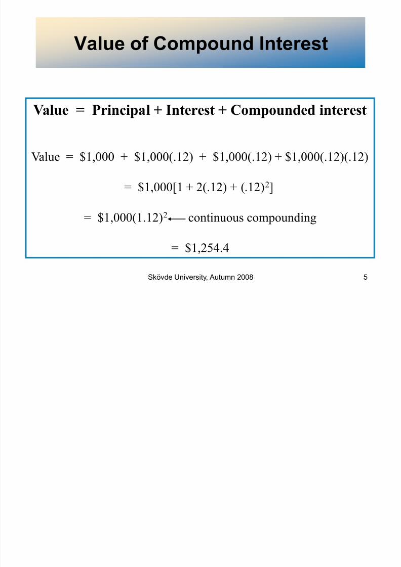
Value of Compound Interest
Value = Principal + Interest + Compounded interest
Value = $1,000 + $1,000(.12) + $1,000(.12) + $1,000(.12)(.12)
= $1,000[1 + 2(.12) + (.12)2]
= $1,000(1.12)2 continuous compounding
= $1,254.4
8/8/2019 FMAI Chapter 2-Lecture 1
http://slidepdf.com/reader/full/fmai-chapter-2-lecture-1 6/37
Skövde University, Autumn 2008 6
Present Value of a Lump Sum Payment
PV function converts future cash flowsinto an equivalent present value bydiscounting future cash flows back tothe present using current marketinterest rate
± lump sum payment
±annuity
PV decreases as interest rates increase:the discount rate is higher for theforeseeable future.

8/8/2019 FMAI Chapter 2-Lecture 1
http://slidepdf.com/reader/full/fmai-chapter-2-lecture-1 7/37
Skövde University, Autumn 2008 7
Calculating Present Value (PV) of aLump Sum payment
PV = FVt (1/(1 + i ))t = FVt (PVIFit )where:
PV = present value
FV = future value (lump sum) received in t years
i = simple annual interest rate earned
t = number of years in the investment horizon
PVIF = present value interest factor of a lump sum

8/8/2019 FMAI Chapter 2-Lecture 1
http://slidepdf.com/reader/full/fmai-chapter-2-lecture-1 8/37
Skövde University, Autumn 2008 8
Calculating Present Value (PV) of a Lump Sumwith multiple interest payment per year
PV = FVn(1/(1 + i/m))nm = FV
n(PVIFi/m,nm)
where:
PV = present value
FV = future value (lump sum) received in n years
i = simple annual interest rate earned
n = number of years in investment horizon
m = number of compounding periods in a year
i/m = periodic rate earned on investments
nm = total number of compounding periods
PVIF = present value interest factor of a lump sum

8/8/2019 FMAI Chapter 2-Lecture 1
http://slidepdf.com/reader/full/fmai-chapter-2-lecture-1 9/37
Skövde University, Autumn 2008 9
Calculating Present Value of aLump Sum
You are offered a security investment thatpays $10,000 at the end of 6 years in exchangefor a fixed payment today.
PV = FVn /(1 + i/m)nm =FV(PVIFi/m,nm)
8% interest PV= $10,000 /(1+0,08)6 = $6,301.70
12% interest PV= $10,000 /(1+0,12)6 = $5,066.31
16% interest PV= $10,000 /(1+0,16)6 = $4,104.42
8/8/2019 FMAI Chapter 2-Lecture 1
http://slidepdf.com/reader/full/fmai-chapter-2-lecture-1 10/37
Skövde University, Autumn 2008 10
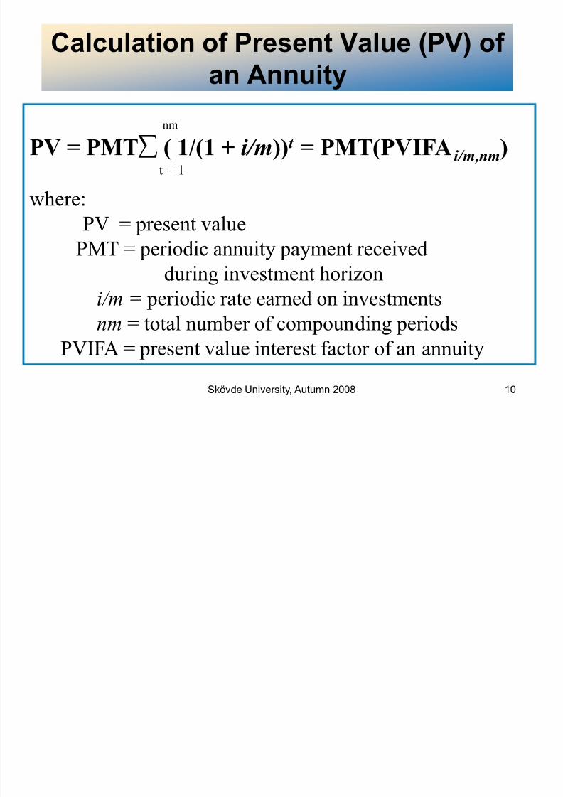
Calculation of Present Value (PV) of an Annuity
nm
PV = PMT§ ( 1/(1 + i/m))t = PMT(PVIFA i/m,nm)t = 1
where:PV = present value
PMT = periodic annuity payment received
during investment horizon
i/m = periodic rate earned on investmentsnm = total number of compounding periods
PVIFA = present value interest factor of an annuity
8/8/2019 FMAI Chapter 2-Lecture 1
http://slidepdf.com/reader/full/fmai-chapter-2-lecture-1 11/37
Skövde University, Autumn 2008 11
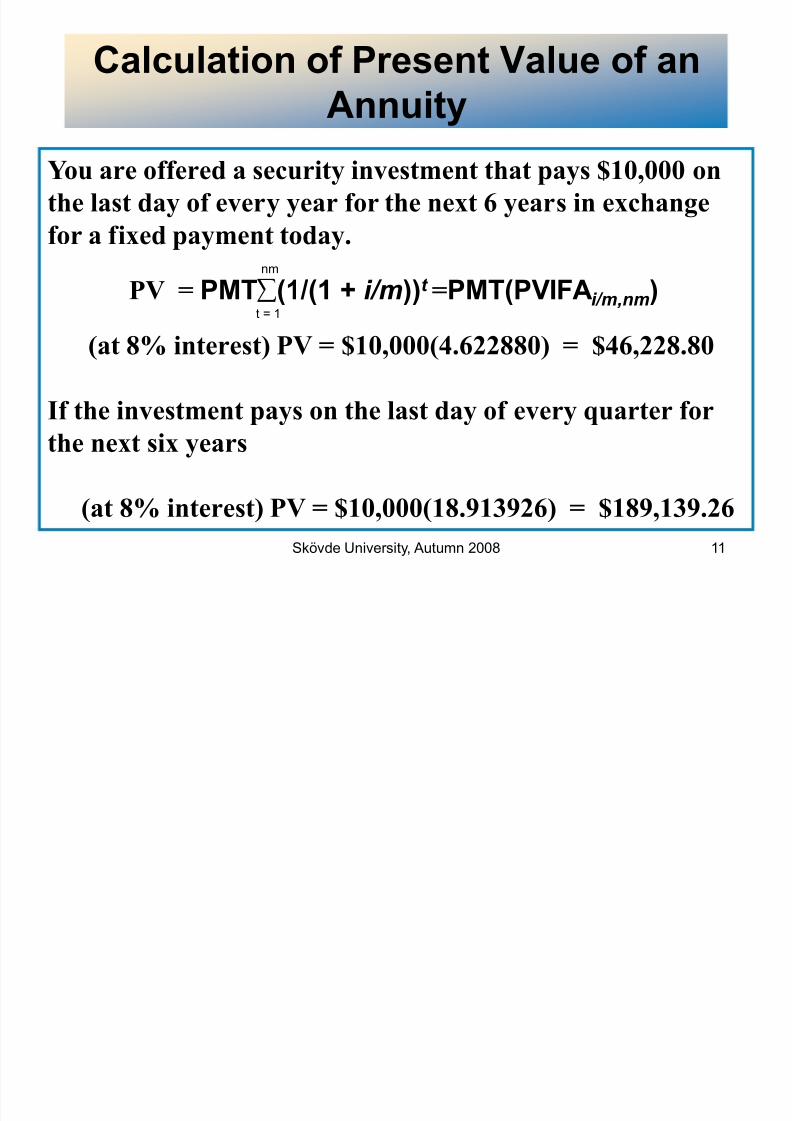
Calculation of Present Value of anAnnuity
You are offered a security investment that pays $10,000 on
the last day of every year for the next 6 years in exchange
for a fixed payment today.nm
PV = PMT§(1 /(1 + i/m))t =PMT(PVIFAi/m,nm)t = 1
(at 8% interest) PV = $10,000(4.622880) = $46,228.80
If the investment pays on the last day of every quarter forthe next six years
(at 8% interest) PV = $10,000(18.913926) = $189,139.26

8/8/2019 FMAI Chapter 2-Lecture 1
http://slidepdf.com/reader/full/fmai-chapter-2-lecture-1 12/37
Skövde University, Autumn 2008 12
Future Values Equations
FV of lump sum equation
FVn = PV(1 + i/m)nm = PV(FVIF i/m, nm)
FV of annuity payment equation
nm-1
FVn = PMT § (1 + i/m)t = PMT(FVIFAi/m, mn)t = 0
Note: the last value paid on Annuity pays no interest.

8/8/2019 FMAI Chapter 2-Lecture 1
http://slidepdf.com/reader/full/fmai-chapter-2-lecture-1 13/37
Skövde University, Autumn 2008 13
Relation between Interest Ratesand Present and Future Values
PresentValue
(PV)
Interest Rate
Future
Value(FV)
Interest Rate
8/8/2019 FMAI Chapter 2-Lecture 1
http://slidepdf.com/reader/full/fmai-chapter-2-lecture-1 14/37
Skövde University, Autumn 2008 14
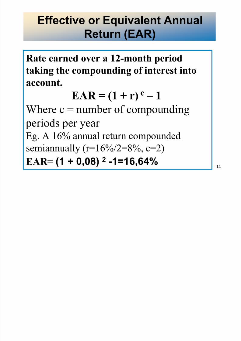
Effective or Equivalent AnnualReturn (EAR)
Rate earned over a 12-month period
taking the compounding of interest into
account.EAR = (1 + r) c ± 1
Where c = number of compounding
periods per year Eg. A 16% annual return compounded
semiannually (r=16%/2=8%, c=2)
EAR = (1 + 0,08) 2 -1=16,64%

8/8/2019 FMAI Chapter 2-Lecture 1
http://slidepdf.com/reader/full/fmai-chapter-2-lecture-1 15/37
Skövde University, Autumn 2008 15
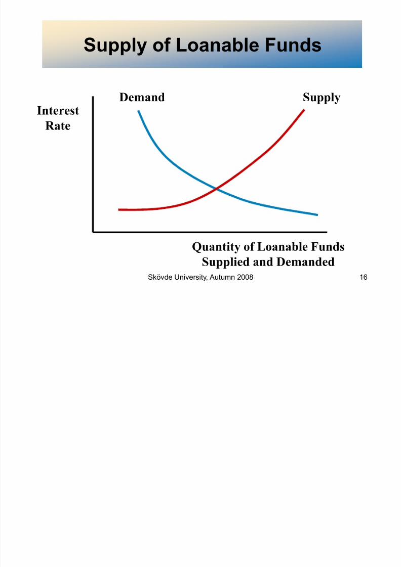
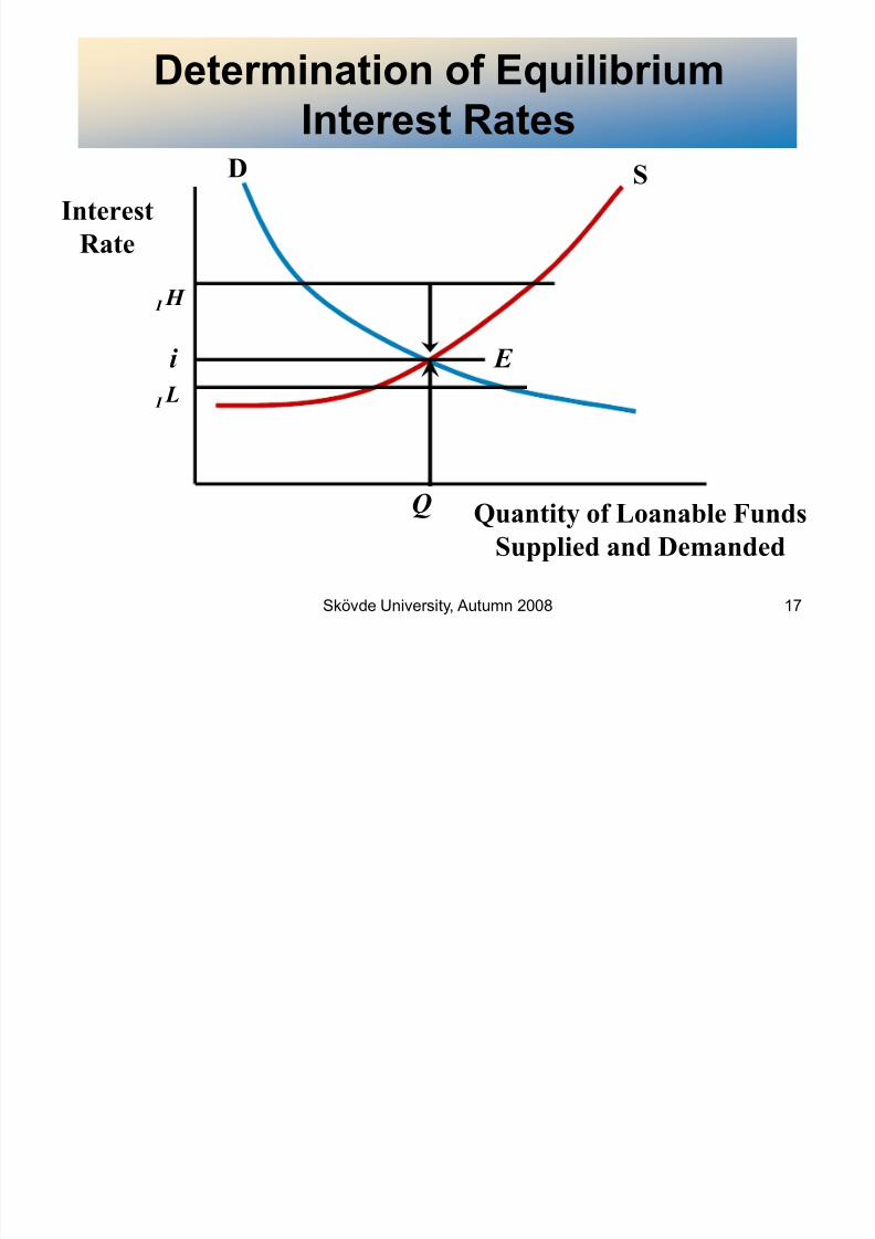
Loanable Funds Theory
A theory of interest rate determinationthat views equilibrium interest rates in
financial markets as a result of thesupply and demand for loanable funds
8/8/2019 FMAI Chapter 2-Lecture 1
http://slidepdf.com/reader/full/fmai-chapter-2-lecture-1 16/37
8/8/2019 FMAI Chapter 2-Lecture 1
http://slidepdf.com/reader/full/fmai-chapter-2-lecture-1 17/37
Skövde University, Autumn 2008 17
Determination of EquilibriumInterest Rates
Interest
Rate
Quantity of Loanable Funds
Supplied and Demanded
D S
I H
i
I L
E
Q
8/8/2019 FMAI Chapter 2-Lecture 1
http://slidepdf.com/reader/full/fmai-chapter-2-lecture-1 18/37
Skövde University, Autumn 2008 18
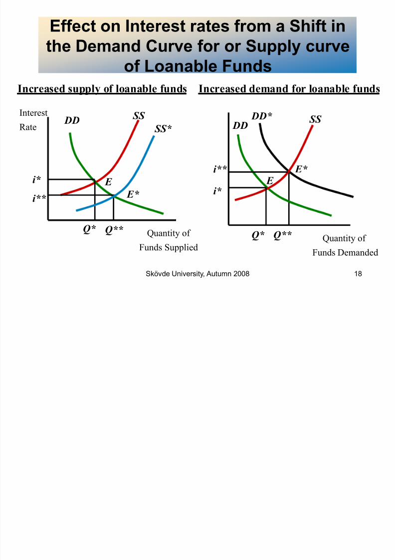
Effect on Interest rates from a Shift inthe Demand Curve for or Supply curve
of Loanable FundsIncreased supply of loanable funds Increased demand for loanable funds
Quantity of
Funds Supplied
Interest
RateDD
SS
SS*
E
E *
Q*
i *
Q**
i **
Quantity of
Funds Demanded
DD
DD* SS
E E *
i *
i **
Q* Q**

8/8/2019 FMAI Chapter 2-Lecture 1
http://slidepdf.com/reader/full/fmai-chapter-2-lecture-1 19/37
Skövde University, Autumn 2008 19
Factors Affecting Nominal InterestRates
Inflation
Real Interest Rate Default Risk
Liquidity Risk
Special Provisions Term to Maturity
8/8/2019 FMAI Chapter 2-Lecture 1
http://slidepdf.com/reader/full/fmai-chapter-2-lecture-1 20/37
Skövde University, Autumn 2008 20
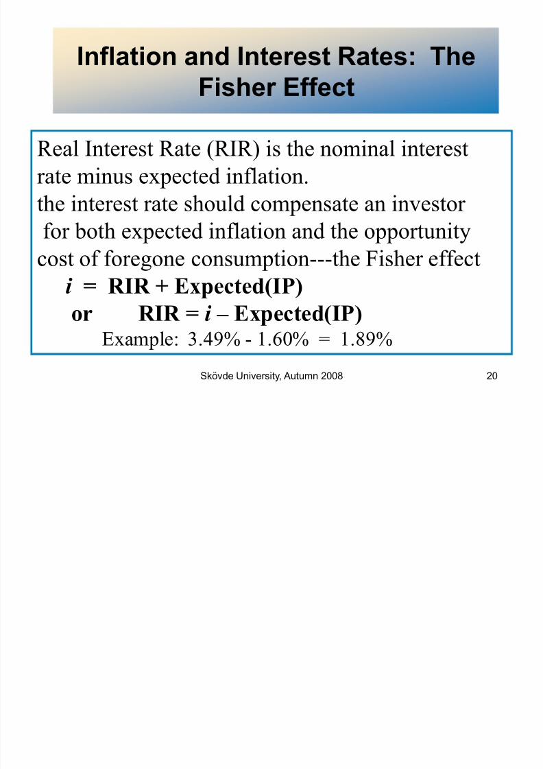
Inflation and Interest Rates: The
Fisher Effect
Real Interest Rate (RIR) is the nominal interest
rate minus expected inflation.
the interest rate should compensate an investor
for both expected inflation and the opportunity
cost of foregone consumption---the Fisher effect
i = RIR + Expected(IP)or RIR = i ± Expected(IP)
Example: 3.49% - 1.60% = 1.89%
8/8/2019 FMAI Chapter 2-Lecture 1
http://slidepdf.com/reader/full/fmai-chapter-2-lecture-1 21/37
Skövde University, Autumn 2008 21
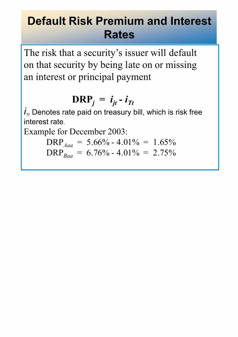
Default Risk Premium and InterestRates
The risk that a security¶s issuer will default
on that security by being late on or missing
an interest or principal payment
DRP j = i j t - i Tt i Tt Denotes rate paid on treasury bill, which is risk free
interest rate.
Example for December 2003:
DRP Aaa = 5.66% - 4.01% = 1.65%
DRP Baa = 6.76% - 4.01% = 2.75%

8/8/2019 FMAI Chapter 2-Lecture 1
http://slidepdf.com/reader/full/fmai-chapter-2-lecture-1 22/37
Skövde University, Autumn 2008 22
Term to Maturity and InterestRates: Yield Curve
Yield to
Maturity
Time to Maturity
(a)
(b)
(c)
(a) Upward sloping
(b) Inverted or downward
sloping
(c) Flat

8/8/2019 FMAI Chapter 2-Lecture 1
http://slidepdf.com/reader/full/fmai-chapter-2-lecture-1 23/37
Skövde University, Autumn 2008 23
Term Structure of Interest Rates
Unbiased Expectations Theory
Liquidity Premium Theory Market Segmentation Theory

8/8/2019 FMAI Chapter 2-Lecture 1
http://slidepdf.com/reader/full/fmai-chapter-2-lecture-1 24/37
Skövde University, Autumn 2008 24
Expectations Theory
Key Assumption: Bonds of different maturities areperfect substitutes
Implication: R e on bonds of different maturities
are equal
Investment strategies for two-period horizon
1. Buy $1 of one-year bond and when matures buy another one-year bond
2. Buy $1 of two-year bond and hold it

8/8/2019 FMAI Chapter 2-Lecture 1
http://slidepdf.com/reader/full/fmai-chapter-2-lecture-1 25/37
Skövde University, Autumn 2008 25
Expectations Theory
Investment strategies for two-period
horizon
1. Buy $1 of one-year bond and whenmatures buy another one-year bond
2. Buy $1 of two-year bond and hold it
8/8/2019 FMAI Chapter 2-Lecture 1
http://slidepdf.com/reader/full/fmai-chapter-2-lecture-1 26/37
Skövde University, Autumn 2008 26
it
!it
it 1 i
t 2 ... it 1
n
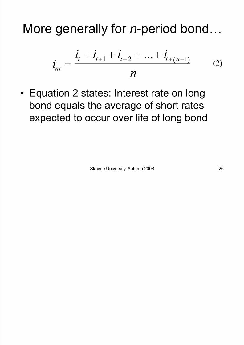
More generally for n-period bond«
Equation 2 states: Interest rate on longbond equals the average of short ratesexpected to occur over life of long bond
(2)
8/8/2019 FMAI Chapter 2-Lecture 1
http://slidepdf.com/reader/full/fmai-chapter-2-lecture-1 27/37
Skövde University, Autumn 2008 27
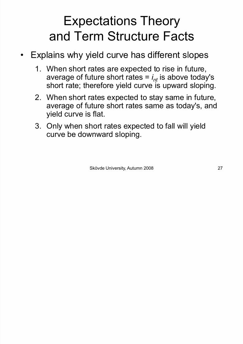
Expectations Theoryand Term Structure Facts
Explains why yield curve has different slopes
1. When short rates are expected to rise in future,average of future short rates = i
nt is above today's
short rate; therefore yield curve is upward sloping.2. When short rates expected to stay same in future,
average of future short rates same as today's, andyield curve is flat.
3. Only when short rates expected to fall will yieldcurve be downward sloping.

8/8/2019 FMAI Chapter 2-Lecture 1
http://slidepdf.com/reader/full/fmai-chapter-2-lecture-1 28/37
Skövde University, Autumn 2008 28
Market Segmentation Theory
Key Assumption: Bonds of different maturities arenot substitutes at all
Implication: Markets are completely
segmented; interest rate at each maturity determinedseparately

8/8/2019 FMAI Chapter 2-Lecture 1
http://slidepdf.com/reader/full/fmai-chapter-2-lecture-1 29/37
Skövde University, Autumn 2008 29
Market Segmentation Theory
Explains fact 3²that yield curve is usuallyupward sloping ± People typically prefer short holding periods and thus have
higher demand for short-term bonds, which have higher prices and lower interest rates than long bonds
Does not explain fact 1 or fact 2 because itsassumes long-term and short-term rates aredetermined independently

8/8/2019 FMAI Chapter 2-Lecture 1
http://slidepdf.com/reader/full/fmai-chapter-2-lecture-1 30/37
Skövde University, Autumn 2008 30
Liquidity Premium Theory
Key Assumption: Bonds of different maturitiesare substitutes, but are notperfect substitutes
Implication: Modifies ExpectationsTheory with features of MarketSegmentation Theory
8/8/2019 FMAI Chapter 2-Lecture 1
http://slidepdf.com/reader/full/fmai-chapter-2-lecture-1 31/37
Skövde University, Autumn 2008 31
i
t !
it
it 1
e
it 2
e
... it 1
e
n
lnt
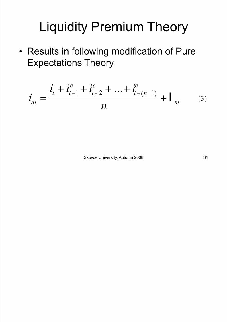
Liquidity Premium Theory
Results in following modification of PureExpectations Theory
(3)
8/8/2019 FMAI Chapter 2-Lecture 1
http://slidepdf.com/reader/full/fmai-chapter-2-lecture-1 32/37
Skövde University, Autumn 2008 32
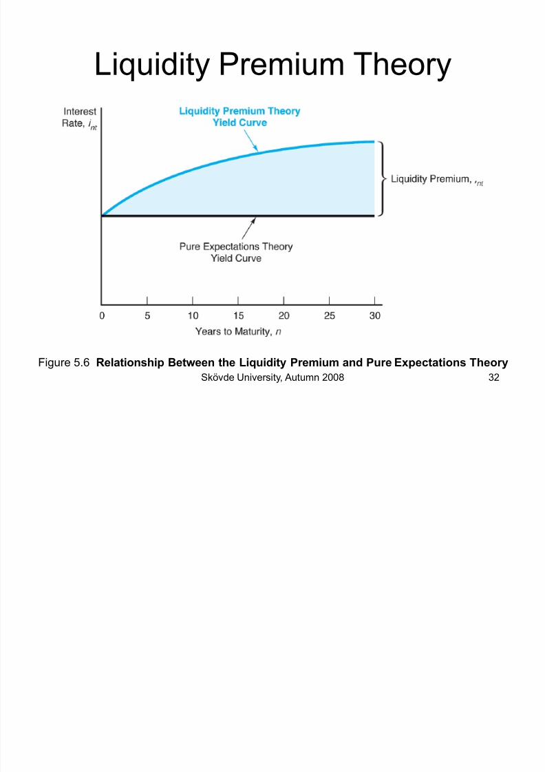
Figure 5.6 Relationship Between the Liquidity Premium and Pure Expectations Theory
Liquidity Premium Theory

8/8/2019 FMAI Chapter 2-Lecture 1
http://slidepdf.com/reader/full/fmai-chapter-2-lecture-1 33/37
Skövde University, Autumn 2008 33
Forecasting Interest Rates
Forward rate is an expected or ³implied´ rate
on a security that is to be originated at some
point in the future using the unbiased
expectations theory _ _
1R 2 = [(1 + 1R 1)(1 + (2f 1))]1/2 - 1
where 2f 1 = expected one-year rate for year 2, or the implied
_ _ forward one-year rate for next year 2f 1=[(1+ 1R2 )2 /(1+1R1)]-1

8/8/2019 FMAI Chapter 2-Lecture 1
http://slidepdf.com/reader/full/fmai-chapter-2-lecture-1 34/37
Skövde University, Autumn 2008 34
Present Value of Cash Flows:Example

8/8/2019 FMAI Chapter 2-Lecture 1
http://slidepdf.com/reader/full/fmai-chapter-2-lecture-1 35/37
Skövde University, Autumn 2008 35
U.S. Real and Nominal InterestRates
Figure 3-1 Real and Nominal Interest Rates (Three-Month Treasury Bill), 1953±2004Sample of current rates and indexeshttp://www.martincapital.com/charts.htm
8/8/2019 FMAI Chapter 2-Lecture 1
http://slidepdf.com/reader/full/fmai-chapter-2-lecture-1 36/37
Skövde University, Autumn 2008 36
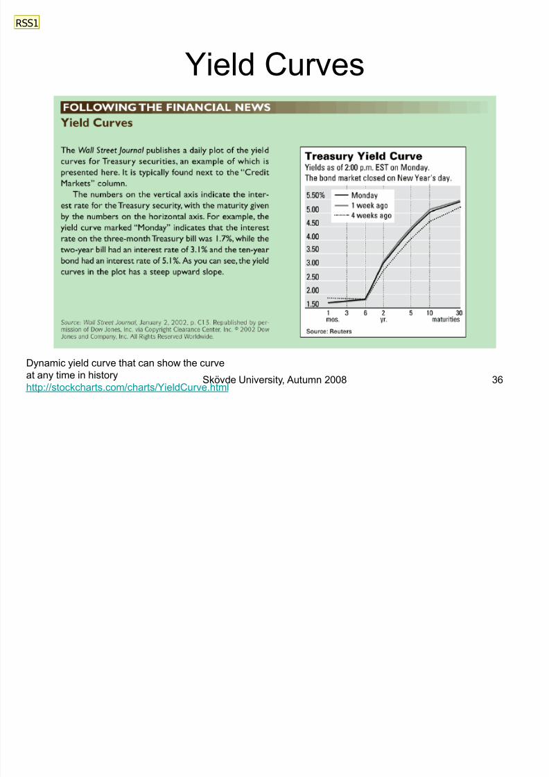
Yield Curves
Dynamic yield curve that can show the curveat any time in history
http://stockcharts.com/charts/YieldCurve.html
RSS1

8/8/2019 FMAI Chapter 2-Lecture 1
http://slidepdf.com/reader/full/fmai-chapter-2-lecture-1 37/37
Slide 36
RSS1 Change title to: Reading the Wall St. JournalRick Swasey, 12/12/2004