financial times series - math.chalmers.se
TRANSCRIPT

Financial Times Series
Lecture 7

Regime Switching
• We sometimes talk about bull and bear markets
• By bull market we mean a market where prices are increasing and where volatility is relatively low
• By bear market we mean a market where prices are decreasing and where volatility is relatively high

Regime Switching
• So if we would like to model log-returns under the assumption that the market switches between the bull and bear states we let
𝑟𝑡 = 𝜇𝑏𝑢𝑙𝑙 + 𝜎𝑏𝑢𝑙𝑙𝜀𝑡, 𝑠𝑡= 𝑏𝑢𝑙𝑙𝜇𝑏𝑒𝑎𝑟 + 𝜎𝑏𝑒𝑎𝑟𝜀𝑡, 𝑠𝑡= 𝑏𝑒𝑎𝑟
• Here 𝑠𝑡 denotes the state of the market at time 𝑡 and 𝜀𝑡 is i.i.d 𝑁 0,1

Regime Switching
• Typically we cannot tell what state the market is in but using some filtering techniques and assumptions on the switching mechanism we can estimate switching probabilities, drifts and volatilities
• We may assume that the switching between the states is Markovian, i.e. the probability of switching from one state to another depends only on which state the market is in a the time point of switching and not on in which states the market has been in or returns at previous time points
𝑃 𝑠𝑡|𝑠𝑡−1 = 𝑃 𝑠𝑡|𝑠𝑡−1, 𝑠𝑡−2, … , 𝑟𝑡−1, 𝑟𝑡−2, …

Regime Switching
• If we denote the market states 0 and 1 we let
𝑝00 = 𝑃 𝑠𝑡 = 0|𝑠𝑡−1 = 0 𝑝01 = 𝑃 𝑠𝑡 = 1|𝑠𝑡−1 = 0 𝑝10 = 𝑃 𝑠𝑡 = 0|𝑠𝑡−1 = 1 𝑝11 = 𝑃 𝑠𝑡 = 1|𝑠𝑡−1 = 1
• Clearly 𝑝00 = 1 − 𝑝01 and 𝑝11 = 1 − 𝑝10

Estimation
• So given a series of observations 𝑟1, … , 𝑟𝑇 we want to estimate the parameters 𝜃 = 𝑝00, 𝑝11, 𝜇0, 𝜇1, 𝜎0, 𝜎1
• Since we cannot tell which state we are in at a given time point it is not obvious how the estimations can be done but we may formally write the likelihood function
𝐿 𝜃 = 𝑓 𝑟1|𝜃 𝑓 𝑟2|𝜃, 𝑟1 ⋯𝑓 𝑟𝑇|𝜃, 𝑟1, … , 𝑟𝑇−1
where 𝑓 is the density of a 𝑁 𝜇𝑠, 𝜎𝑠2 random variable

Estimation
• So the contribution of 𝑟𝑡 to the log-likelihood is
log𝑓 𝑟𝑡|𝜃, 𝑟1, … , 𝑟𝑡−1
• Using conditional probabilities and the Markov property, we can write (exercise)
𝑓 𝑠𝑡 , 𝑠𝑡−1, 𝑟𝑡|𝜃, 𝑟1, … , 𝑟𝑡−1= 𝑓 𝑠𝑡−1|𝜃, 𝑟1, … , 𝑟𝑡−1 𝑓 𝑠𝑡|𝑠𝑡−1, 𝜃 𝑓 𝑟𝑡|𝑠𝑡 , 𝜃

Estimation
• Above 𝑓 𝑠𝑡|𝑠𝑡−1, 𝜃 is the switching probability and
𝑓 𝑟𝑡|𝑠𝑡, 𝜃 =1
2𝜋𝜎𝑠𝑡𝑒𝑥𝑝 −
1
2
𝑟𝑡−𝜇𝑠𝑡𝜎𝑠𝑡
2
• The function 𝑓 𝑠𝑡−1|𝜃, 𝑟1, … , 𝑟𝑡−1 is given by
𝑓 𝑠𝑡−1,𝑠𝑡−2=0,𝑟𝑡−1|𝜃,𝑟1,…,𝑟𝑡−2 +𝑓 𝑠𝑡−1,𝑠𝑡−2=1,𝑟𝑡−1|𝜃,𝑟1,…,𝑟𝑡−2
𝑓 𝑟𝑡−1|𝜃,𝑟1,…,𝑟𝑡−2

Estimation
• So we get
𝑓 𝑟𝑡|𝜃, 𝑟1, … , 𝑟𝑡−1 = 𝑓 𝑠𝑡 = 𝑖, 𝑠𝑡−1 = 𝑗, 𝑟𝑡|𝜃, 𝑟1, … , 𝑟𝑡−1
2
𝑗=1
2
𝑖=1
• To start the recursion we may let
𝑓 𝑠1 = 0, 𝑟1|𝜃 =1
2
1
2𝜋𝜎0𝑒𝑥𝑝 −
1
2
𝑟1 − 𝜇0𝜎0
2
𝑓 𝑠1 = 1, 𝑟1|𝜃 =1
2
1
2𝜋𝜎1𝑒𝑥𝑝 −
1
2
𝑟1 − 𝜇1𝜎1
2

Estimation
• This gives
𝑓 𝑟1|𝜃 = 𝑓 𝑠1 = 0, 𝑟1|𝜃 + 𝑓 𝑠1 = 1, 𝑟1|𝜃
• and
𝑓 𝑠1 = 0|𝜃, 𝑟1 =𝑓 𝑠1 = 0, 𝑟1|𝜃
𝑓 𝑟1|𝜃
𝑓 𝑠1 = 1|𝜃, 𝑟1 =𝑓 𝑠1 = 1, 𝑟1|𝜃
𝑓 𝑟1|𝜃

Estimation
• Next we get
𝑓 𝑟2|𝜃, 𝑟1 = 𝑓 𝑠1 = 𝑖, 𝑠2 = 𝑗, 𝑟2|𝜃, 𝑟1
2
𝑗=1
2
𝑖=1
• where
𝑓 𝑠1 = 𝑖, 𝑠2 = 𝑗, 𝑟2|𝜃, 𝑟1
= 𝑓 𝑠1 = 𝑖|𝜃, 𝑟1 𝑝𝑗𝑖1
2𝜋𝜎𝑗𝑒𝑥𝑝 −
1
2
𝑟2 − 𝜇𝑗
𝜎𝑗
2
• And so forth…

Estimation
• So, the maximization of the likelihood-function cannot be done manually but using standard routines like fminsearch or fmincon in matlab we can find our parameter estimates
• There is a matlab package by Marcelo Perlin called MS_Regress available online (for free) that does the parameter estimation and then some…

For the ^N225
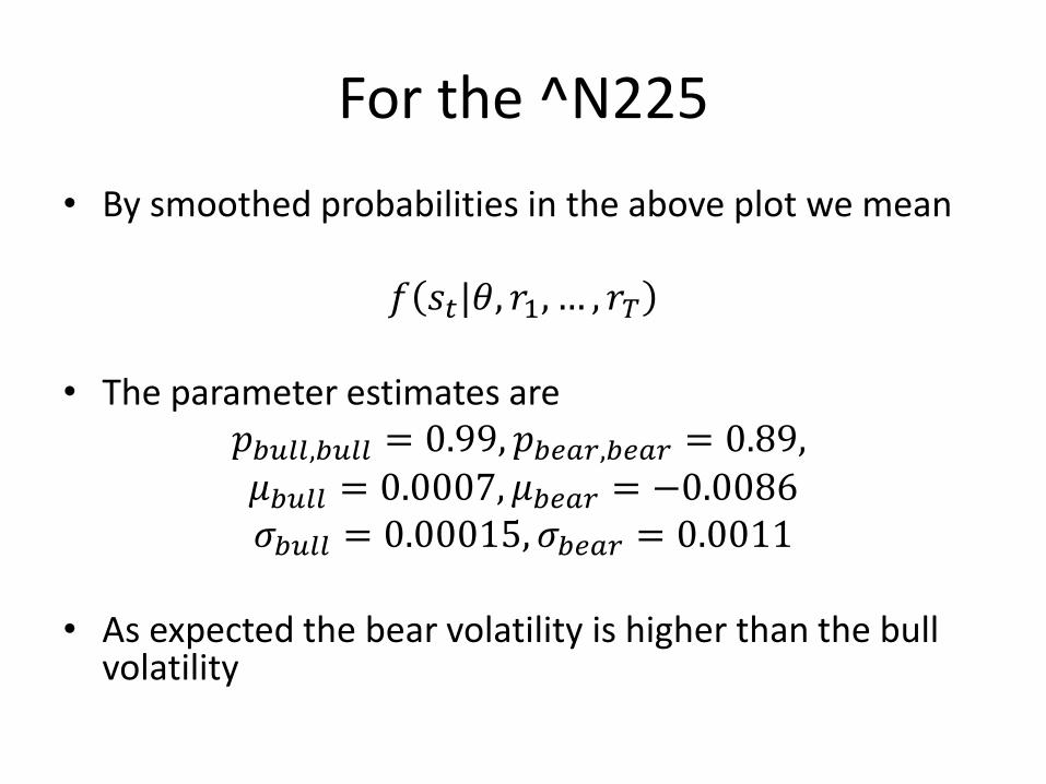
For the ^N225
• By smoothed probabilities in the above plot we mean
𝑓 𝑠𝑡|𝜃, 𝑟1, … , 𝑟𝑇
• The parameter estimates are 𝑝𝑏𝑢𝑙𝑙,𝑏𝑢𝑙𝑙 = 0.99, 𝑝𝑏𝑒𝑎𝑟,𝑏𝑒𝑎𝑟 = 0.89, 𝜇𝑏𝑢𝑙𝑙 = 0.0007, 𝜇𝑏𝑒𝑎𝑟 = −0.0086 𝜎𝑏𝑢𝑙𝑙 = 0.00015, 𝜎𝑏𝑒𝑎𝑟 = 0.0011
• As expected the bear volatility is higher than the bull
volatility

Non-parametric models
• What if we do not make any distribution assumptions?
• Assume that 𝑟𝑡 and 𝑥𝑡 are two time series for which we want to explore their relationship
• Maybe it is possible to fit a model
𝑟𝑡 = 𝑚 𝑥𝑡 + 𝑎𝑡 where 𝑚 is some smooth function to be estimated from the data

Non-parametric models
• If we had independent observerations 𝑟1, … , 𝑟𝑇 for a fixed 𝑥𝑡 = 𝑥 the we could write
𝑟𝑡𝑇𝑡=1
𝑇= 𝑚 𝑥 +
𝑎𝑡𝑇𝑡=1
𝑇
• For a sufficiently large 𝑇 the mean of the noise (LLN)
will be close to zero so in this case
𝑚 𝑥 = 𝑟𝑡𝑇𝑡=1
𝑇
Non-parametric models
• In financial applications we will typically not have data as above. Rather we will have pairs of observations
𝑟1, 𝑥1 , … , 𝑟𝑇 , 𝑥𝑇
• But if the function 𝑚 is sufficiently smooth then a
value of 𝑟𝑡 for which 𝑥𝑡 ≈ 𝑥 will still give a good approximation of 𝑚 𝑥
• For a value of 𝑟𝑡 for which 𝑥𝑡 is not close to 𝑥 will give a less accurate approximation of 𝑚 𝑥

Non-parametric models
• So instead of a simple average, we use a weighted average
𝑚 𝑥 =1
𝑇 𝑤𝑡(𝑥)𝑟𝑡
𝑇
𝑡=1
where the weights 𝑤𝑡(𝑥) are large for those 𝑟𝑡 with 𝑥𝑡 close to 𝑥 and weights are small for 𝑟𝑡 with 𝑥𝑡 not close to 𝑥

Non-parametric models • Above we assume that 𝑤𝑡 𝑥 = 𝑇𝑇
𝑡=1
• One may also treat 1
𝑇 as part of the weights and work
under the assumption 𝑤𝑡 𝑥 = 1𝑇𝑡=1
• A construction like the one at hand where we will let the weights depend on a choice of measure for the distance between 𝑥𝑡 and 𝑥 and the size of the weights depends on the distance may be referred to as a local weighted average

Kernel regression
• One way of finding appropriate weights is to use kernels 𝐾 𝑥 which are typically probability density functions
𝐾(𝑥) ≥ 0 and 𝐾 𝑥 𝑑𝑥 = 1∞
−∞
• For flexibility we will allow scaling of the kernel using a ”bandwidth” ℎ
𝐾ℎ 𝑥 =1
ℎ𝐾 𝑥 ℎ , 𝐾ℎ 𝑥 𝑑𝑥 = 1
∞
−∞
• The weights may be defined as
𝑤𝑡 𝑥 =𝐾ℎ 𝑥 − 𝑥𝑡
𝐾ℎ 𝑥 − 𝑥𝑡𝑇𝑡=1

Nadaraya-Watson
• The N-W kernel estimator (N-W 1964) is given by
𝑚 𝑥 = 𝑤𝑡(𝑥)𝑟𝑡
𝑇
𝑡=1
= 𝐾ℎ 𝑥 − 𝑥𝑡 𝑟𝑡𝑇𝑡=1
𝐾ℎ 𝑥 − 𝑥𝑡𝑇𝑡=1
• The choice of kernel is often (Gaussian)
𝐾ℎ 𝑥 =1
ℎ 2𝜋𝑒𝑥𝑝 −
𝑥2
2ℎ2
or (Epanechnikov)
𝐾ℎ 𝑥 =3
4ℎ1 −
𝑥2
ℎ2𝟏 𝑥 ≤ ℎ

What does the bandwidth do?
• If we use the Epanechnikov kernel we get
𝑚 𝑥 = 𝐾ℎ 𝑥 − 𝑥𝑡 𝑟𝑡𝑇𝑡=1
𝐾ℎ 𝑥 − 𝑥𝑡𝑇𝑡=1
= 1 −
𝑥 − 𝑥𝑡2
ℎ2𝟏 𝑥 − 𝑥𝑡 ≤ ℎ 𝑟𝑡
𝑇𝑡=1
1 −𝑥 − 𝑥𝑡
2
ℎ2𝟏 𝑥 − 𝑥𝑡 ≤ ℎ𝑇
𝑡=1
• If ℎ → ∞
𝑚 𝑥 →1
𝑇 𝑟𝑡
𝑇
𝑡=1
and if ℎ → 0
𝑚 𝑥 → 𝑟𝑡 where 𝑟𝑡 is the observation for which 𝑥 − 𝑥𝑡 is smallest within the sample

Bandwidth Selection
• Fan and Yao (2003) suggest
ℎ = 1.06𝑠𝑇−1/5
for the Gaussian Kernel and
ℎ = 2.34𝑠𝑇−1/5
for the Epanechnikov kernel where 𝑠 is the sample standard deviation of 𝑥𝑡 which is assumed stationary

Cross Validation
• Let
𝑚 ℎ,𝑗 𝑥𝑗 =1
𝑇 − 1 𝑤𝑡 𝑥𝑗 𝑦𝑡𝑡≠𝑗
which is an estimate of 𝑦𝑗 where the weights sum to 𝑇 − 1. • Also let
𝐶𝑉 ℎ =1
𝑇 𝑦𝑗 −𝑚 ℎ,𝑗 𝑥𝑗
2𝑊 𝑥𝑗
𝑇
𝑗=1
where 𝑊 ∙ is anonnegative weight function satisfying 𝑊 𝑥𝑗 = 𝑇𝑇𝑗=1

Cross Validation
• The function 𝐶𝑉 ℎ is called the cross-validation function since it validates the ability of the smoother 𝑚 to predict 𝑦𝑡
• The weight function 𝑊 may be chosen to downweight certain observations if necessary
but 𝑊 𝑥𝑗 = 1 is often sufficient

Cross Validation
• It is an exercise to show that
𝐶𝑉 ℎ =1
𝑇 𝑦𝑗 −𝑚 ℎ,𝑗 𝑥𝑗
2𝑇
𝑗=1
=1
𝑇 𝑦𝑗 −𝑚 𝑥𝑗
2/ 1 −
𝐾ℎ 0
𝐾ℎ 𝑥𝑗 − 𝑥𝑖𝑇𝑖=1
2𝑇
𝑗=1

N-W Volatility Estimation
• Assume that 𝑟𝑡 is our log-return series that has been centered at zero so that
𝐸 𝑟2𝑡 = 𝜎2𝑡
• We also assume that 𝑟2𝑡 = 𝜎2𝑡 + 𝜀𝑡 where 𝜀𝑡 is WN

N-W Volatility Estimation
• We may then use the N–W kernel estimator
𝜎 2𝑡 = 𝐾ℎ 𝑡 − 𝑖 𝑟2𝑖𝑡−1𝑖=1
𝐾ℎ 𝑡 − 𝑖𝑡−1𝑖=1
• Below we use Gaussian kernels for OMXS30 data

OMXS30 returns (100104-130412)

OMXS30 N-W volatility estimates
• CV gives ℎ = 23.26 and volatility estimates:

OMXS30 N-W volatility devolatized returns
The Ljung-Box null hypothesis of no autocorrelations cannot be rejected at 5% level p=0.4433

Autocorrelation for devolatized returns

Another application
• Remember the ARIMA example for the Swedish GDP
• What if we try to use N-W to model log GDP 𝑝𝑡 as
𝑝𝑡 = 𝑚 𝑝𝑡−1 + 𝑎𝑡
where 𝑎𝑡 is WN

Log BNP
• Using CV we find ℎ = 0.0367 to be the optimal threshold for the Gaussian kernel and

Residuals
• The seasonality seen using the ARIMA is still left, but we know how to deal with that