financial statement analysis - texas tech...
TRANSCRIPT

Financial Statement Analysis
Hunter Ryffel [email protected]
Micheal Sura [email protected]
Garret Bruce [email protected]
Joe Brewer [email protected]
Jesse Ricones [email protected]
Miles Arbuckle [email protected]

2
Table of Contents
Executive Summary ................................................................................................... 8
Industry analysis .................................................................................................. 10
Accounting analysis .............................................................................................. 12
Financial analysis ................................................................................................. 13
Valuation Analysis ................................................................................................ 18
Company Overview ................................................................................................. 20
Industry Overview................................................................................................ 21
Five Forces Model ................................................................................................... 22
Rivalry among Competitors ...................................................................................... 22
Industry Growth Rate ........................................................................................... 23
Industry Concentration ......................................................................................... 24
Fixed-to-Variable Costs ......................................................................................... 24
Switching Costs ................................................................................................... 25
Exit Barriers ......................................................................................................... 26
Conclusion ........................................................................................................... 26
Threat of New Entrants ........................................................................................... 26
Barriers to Entry .................................................................................................. 27
Distribution Access and Relationships .................................................................... 27
Conclusion ........................................................................................................... 27
Threat of Substitutes ............................................................................................... 28
Relative Price and Performance ............................................................................. 28
Conclusion ........................................................................................................... 28

3
Bargaining Power of Suppliers ................................................................................. 29
Supplier Concentration ......................................................................................... 29
Conclusion ........................................................................................................... 30
Bargaining Power of Customers ............................................................................... 30
Competitor Concentration ..................................................................................... 30
Conclusion ........................................................................................................... 30
Porter’s Five Forces Conclusion ................................................................................ 31
Key Success Factors ................................................................................................ 32
Industry’s Competitive Advantages ....................................................................... 33
Low Input Costs ................................................................................................... 33
Low Distribution Costs .......................................................................................... 33
Efficient Production .............................................................................................. 34
Flexible Delivery ................................................................................................... 34
Conclusion ........................................................................................................... 34
AptarGroup’s Competitive Advantages ................................................................... 35
Production Process ............................................................................................... 35
Geographic Diversity ............................................................................................ 35
Local Production .................................................................................................. 36
Accounting Analysis................................................................................................. 36
Type One Accounting Policies ............................................................................... 37
Low Input Costs ................................................................................................... 37
Low Distribution Costs .......................................................................................... 38
Efficient Production .............................................................................................. 39
Type Two Accounting Policies ............................................................................... 39

4
Goodwill .............................................................................................................. 40
Research and Development .................................................................................. 40
Foreign conversion risk ......................................................................................... 41
Operating leases .................................................................................................. 42
Conclusion ........................................................................................................... 42
Accounting Flexibility Assessment ............................................................................ 43
Goodwill .............................................................................................................. 43
Research and Development .................................................................................. 44
Capital vs. Operating Leases ................................................................................. 44
Conclusion ........................................................................................................... 45
Evaluation of Actual Accounting Strategy .................................................................. 45
Goodwill .............................................................................................................. 46
Research & Development ..................................................................................... 46
Operating Leases ................................................................................................. 47
Quality of Disclosure - Type One .............................................................................. 48
Efficient Production .............................................................................................. 48
Low Input Costs ................................................................................................... 49
Distribution Costs ................................................................................................. 49
Quality of Disclosure – Type Two ............................................................................. 50
Goodwill .............................................................................................................. 50
Research and Development .................................................................................. 51
Foreign Conversion Risk ....................................................................................... 51
Operating Leases ................................................................................................. 52
Potential “Red Flags” ............................................................................................... 52

5
Goodwill .............................................................................................................. 53
Research & Development ..................................................................................... 53
Conclusion ........................................................................................................... 54
Financial Statements ............................................................................................... 54
Balance sheets ..................................................................................................... 54
Income statements .............................................................................................. 57
Conclusion ........................................................................................................... 59
Financial Analysis .................................................................................................... 59
Liquidity Ratios ....................................................................................................... 59
Current Ratio ....................................................................................................... 60
Quick Asset Ratio ................................................................................................. 62
Conclusion ........................................................................................................... 63
Operating Efficiency Ratios ...................................................................................... 63
Inventory Turnover .............................................................................................. 64
Accounts Receivable Turnover .............................................................................. 65
Working Capital Turnover ..................................................................................... 67
Days Supply of Inventory ..................................................................................... 68
Days Sales Outstanding ........................................................................................ 69
Cash to Cash Cycle .............................................................................................. 71
Conclusion ........................................................................................................... 72
Profitability Ratios ................................................................................................... 73
Annual Sales Growth ............................................................................................ 73
Gross Profit Margin .............................................................................................. 74
Operating Profit Margin ........................................................................................ 76

6
Net Profit Margin.................................................................................................. 78
Asset Turnover .................................................................................................... 79
Return on Assets.................................................................................................. 81
Return on Equity .................................................................................................. 82
Conclusion ........................................................................................................... 83
Capital Structure Ratios ........................................................................................... 84
Debt to Equity Ratio ............................................................................................. 84
Times Interest Earned .......................................................................................... 85
Debt Service Margin ............................................................................................. 87
Altman Z-Score .................................................................................................... 88
Internal Growth Rate ........................................................................................... 89
Sustainable Growth Rate ...................................................................................... 91
Conclusion ........................................................................................................... 92
Cost of Capital Estimation ........................................................................................ 92
Cost of Equity ...................................................................................................... 92
Backdoor Cost of Equity ....................................................................................... 94
Cost of Debt ........................................................................................................ 95
WACC (Weighted Average Cost of Capital) ............................................................ 96
Conclusion ........................................................................................................... 97
Forecasting Financial Statements ............................................................................. 97
Income Statement ............................................................................................... 98
Dividends Forecasting .......................................................................................... 99
Balance Sheet ...................................................................................................... 99
Cash Flow Statement ......................................................................................... 100

7
Method of Comparables ......................................................................................... 101
Price to Earnings (P/E) Trailing ........................................................................... 101
Price to Earnings (P/E) Forecast .......................................................................... 102
Price to Book ..................................................................................................... 102
Dividends to Price .............................................................................................. 103
Price to Earnings Growth (PEG) .......................................................................... 104
Price to EBITDA ................................................................................................. 104
Price to Free Cash Flow ...................................................................................... 104
Enterprise Value to EBITDA ................................................................................ 105
Price to Sales ..................................................................................................... 105
Conclusion ......................................................................................................... 106
Intrinsic Model Valuation ....................................................................................... 106
Discounted Dividends Model ............................................................................... 107
Discounted Free Cash Flow Model ....................................................................... 108
Residual Income Model ...................................................................................... 109
Long-Run Residual Income Model ....................................................................... 110
Intrinsic Valuation Model Conclusion ................................................................... 112
APPENDIX ............................................................................................................ 113
References ........................................................................................................ 113
Forecasted Financial Statements ......................................................................... 113

8
Executive Summary
Analyst Recommendation: Don’t buy (Overvalued)
April 1st, 2016
Observed Price 2011 2012 2013 2014 201552 Week Range Scores 4.366 4.404 4.374 4.573 4.018RevenueMarket CapitalizationShares Outstanding
As Stated Restated ValuedTrailing P/E 31.94 32.65 Overvalued
Return on Equity Forward P/E 21.19 22.87 OvervaluedReturn on Assets Price to Book 3.83 4.05 Overvalued
Dividend to Price 0.02 0.01 UndervaluedRegression Beta P.E.G. Ratio 2.55 2.78 Overvalued24 months 0.93 Price to EBITDA 59.67 62.03 Overvalued36 months 0.96 Price to FCF 154.89 N/A N/A48 months 0.99 EV/EBITDA 71.87 69.56 Undervalued60 months 0.91 Price to Sales 89.45 91.23 Overvalued72 months 0.93
As Stated Valued$28.78 Overvalued
Actual Lower Upper Free Cash Flows $34.97 OvervaluedCost of Equity 9.75% 8.43% 11.07% Residual Income $24.35 UndervaluedWACCBT 6.70% 6.07% 7.32% $26.13 OvervaluedWACCAT 6.02% 5.40% 6.64%
Cost of Capital
AptarGroup NYSE (04/1/2016) Altman Z-Scores$67.90
$60.73 - $80.36$2317.15 Million
$4.82 Billion Financial Based Valuations63.16 Million
23%10.90%
Intrinsic Based Valuations
Discounted Dividends
Long Run Residual Income
R Squared51.39%56.30%54.90%53.74%58.60%

9
Figure 1.Error! No text of specified style in document..1 - Share price of AptarGroup in the last five years
Figure Error! No text of specified style in document..2 - Share price of AptarGroup and main competitors

10
Industry analysis
AptarGroup, Inc. (ATR) is a worldwide manufacturer of plastic containers
and lids predominantly for the beauty, healthcare, homecare and prescription
drug markets, and the food and beverage industry.
We have identified Ball Corporation (BLL), Crown Holdings (CCK), and
Silgan Holdings (SLGN) as AptarGroup’s main competitors.
The primary products that AptarGroup produces today are dispensing
pumps, aerosol valves and closures. Dispensing pumps are a convenient
dispensing device and are used for products such as soap and shampoo.
We used the Porter’s Five Forces Model in order to determine the
profitability a firm could expect in the P&C industry.
Five Forces Model
Rivalry Among Existing Firms High
Threat of New Entrants Low
Threat of Substitute Products Medium
Bargaining Power of Customers High
Bargaining Power of Suppliers Low

11
Rivalry among existing firms is very high due to the fact that the P&C
industry is a highly competitive market with both public and private firms
competing locally and internationally to provide high quality low cost products
(ATR, CCK, SLGN 10-K).
The threat of new entrants is low since the industry has high barriers to
entry and requires efficient distribution access. The average firm in the industry
has a market capitalization of $5.39 billion. This is supported by billions in assets,
supporting the statement that new firms would have to be large to be able to
compete.
The threat of substitute products is mixed-high within the industry. In the
P&C industry, the manufacturers produce goods cost-efficiently. It is difficult for
a potential substitute to undercut the market participants. The suppliers can also
protect themselves by the imposing the contractual obligations on customers.
The bargaining power of customers is high. The P&C industry is highly
saturated with local and international competitors. The industry is highly
competitive, allowing customers to set prices. On the other hand, the bargaining
power of suppliers is low due to the large number of suppliers and low switching
costs.
The P&C industry is in the sector of basic materials. The costs in this
sector are low; this focus on low cost output is the result of price-taking behavior

12
of suppliers. We further assume that the industry is a price-taker in our
predictions of the factors that determine the success in the industry.
Accounting analysis
Accounting practices are reviewed and looked at to understand the nature
of the company and the packaging and container industry. It is very important
that we look at the accounting practices due to the flexibility that the Generally
Accepted Accounting Principles (GAAP) allows. The Flexibility of the GAAP on a
company’s financial statements can often hide information that needs to be
known when valuing a company. Many companies are hard to value due to the
lack of the financial statements disclosure. We have to look into the type 1
policies’ quality of disclosure in relation to the key success factors of the
company in comparison to the industry analysis. Then, we look at the type 2
policies which look at the distortion in the area of AptarGroup financial structure.
AptarGroup, Type 1 accounting policies, we evaluated the degree of
disclosure in terms of efficient production, low input costs, and distribution costs.
AptarGroup clearly represents risk in all of these three areas; therefore, type one
policies are not a major concern.
AptarGroup, Type 2 accounting policies, we evaluated operating leases to
find that the P&C industry is not heavily invested in operating leases. Operating

13
leases account for 20% or less of non-current liabilities in the P&C industry.
Since it is a small portion of non-current liabilities, it was not considered to be a
red flag. AptarGroup’s goodwill accounts for 40% of the net fixed assets and was
identified as a potential red flag. Also AptarGroup’s lack of expensing R&D when
the cost is incurred raised another potential red flag.
From the account analysis we find that AptarGroup is not very accurate in
terms of disclosure and lacks enough reliable information for an accurate
evaluation. The lack of disclosure for type 2 accounting policies leads us to the
need of restating the financial statements of AptarGroup to adjust for the
potential red flags in goodwill and the expense of R&D.
Financial analysis
For the purpose of the analysis, we calculated the liquidity, capital
structure, and profitability ratios. We formed liquidity ratio analysis is based on
the current and quick ratios, inventory turnover, days supply inventory, accounts
receivable turnover, accounts receivable days, cash to cash cycle, and working
capital turnover.
Determining the liquidity ratios are a vital step when valuing a firm
because the results can show if a firm has the ability to continue as a going
concern or enough cash to cover debts when a creditor is expecting payment.
14
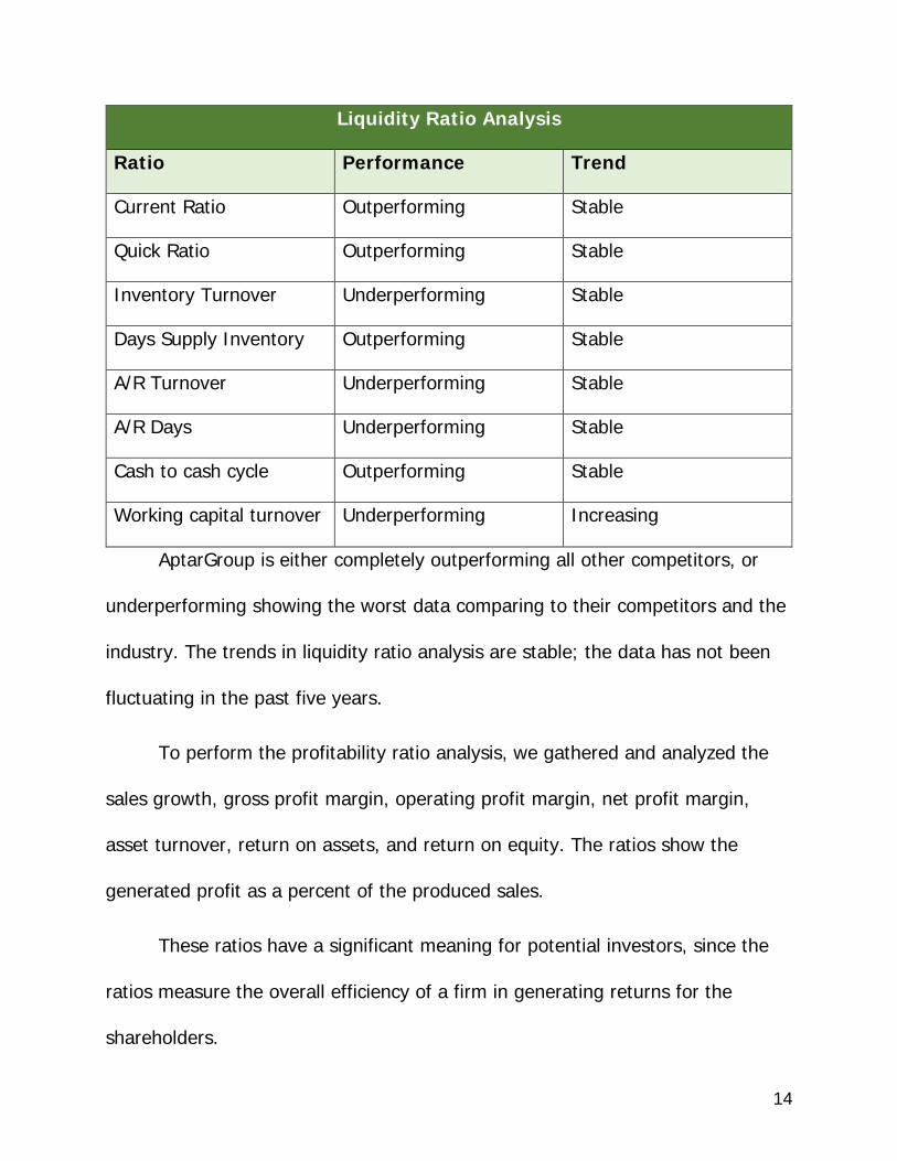
Liquidity Ratio Analysis
Ratio Performance Trend
Current Ratio Outperforming Stable
Quick Ratio Outperforming Stable
Inventory Turnover Underperforming Stable
Days Supply Inventory Outperforming Stable
A/R Turnover Underperforming Stable
A/R Days Underperforming Stable
Cash to cash cycle Outperforming Stable
Working capital turnover Underperforming Increasing
AptarGroup is either completely outperforming all other competitors, or
underperforming showing the worst data comparing to their competitors and the
industry. The trends in liquidity ratio analysis are stable; the data has not been
fluctuating in the past five years.
To perform the profitability ratio analysis, we gathered and analyzed the
sales growth, gross profit margin, operating profit margin, net profit margin,
asset turnover, return on assets, and return on equity. The ratios show the
generated profit as a percent of the produced sales.
These ratios have a significant meaning for potential investors, since the
ratios measure the overall efficiency of a firm in generating returns for the
shareholders.

15
Profitability Ratio Analysis
Ratio Performance Trend
Sales Growth Average Unstable
Gross Profit Margin Outperforming Stable
Net Profit Margin Outperforming Stable
Asset Turnover Average Stable
Return on Assets Outperforming Stable
Return on Equity Average Stable
AptarGroup’s profitability ratios are appealing due to the fact that they are
either outperforming or at the industry’s average.
For the capital structure analysis, we evaluated the debt to equity ratio,
times interest earned, and the Altman’s Z-score. Altman’s Z-score shows whether
the company is heading towards bankruptcy. Since capital structure is the mix of
debt and equity, the debt to equity ratio provides with a better understanding of
the weight of debt and equity.

16
Capital Structure Ratio Analysis
Ratio Performance Trend
Debt to Equity Underperforming Stable
Times Interest Earned Outperforming Decreasing
Altman’s Z-score Average Unstable
After performing the ratio analysis, we forecasted the AptarGroup’ financial
statements. Although financial forecasts cannot be totally accurate, our trends
and ratio analysis help to be able to forecast with a reasonably high accuracy.
We forecasted growth rate, income statement, balance sheet, and the
statement of cash flows. To forecast the growth rate, we started by forecasting
the sales. Since sales growth rate is what drives the income forecast, the
forecast shows the data in accordance with the sales. Our forecasting of the
balance sheet is done through using the forecasting of the asset turnover ratio.
The forecast of the statement of cash flows usually has the lowest accuracy, due
to the fact that the statement of cash flows is the most volatile financial
statement.
Finally, we calculated AptarGroup’s cost of equity and cost of debt that
allowed us to estimate the weighted average cost of capital (WACC). The cost of

17
debt takes into account all interest rates in proportion with the weight that is
allocated to each rate. To estimate cost of equity, we used both the backdoor
cost of equity and the CAPM formula. We further picked the CAPM method as our
main method in finding the cost equity.
We gathered necessary inputs for the CAPM formula from the St. Louis
Federal reserve website and the regression models.
20 year regressions
Months Beta
Beta
LB
Beta
UB R^2 SP MRP Rf Ke Ke LB Ke UB
24 0.932 0.530 1.33 51.39% 1.00% 7.00% 2.25% 9.78% 6.96% 12.59%
36 0.958 0.665 1.25 56.30% 1.00% 7.00% 2.25% 9.96% 7.90% 12.02%
48 0.994 0.726 1.26 54.90% 1.00% 7.00% 2.25% 10.21% 8.33% 12.09%
60 0.905 0.684 1.13 53.74% 1.00% 7.00% 2.25% 9.58% 8.04% 11.13%
72 0.928 0.740 1.12 58.58% 1.00% 7.00% 2.25% 9.75% 8.43% 11.07%
We also provided with the WACC before and after tax. The following table
tells us that AptarGroup pays an average of 6.02 cents for every dollar in their
extra funding.

18
Market
Value
Amount (in
millions) Rate Weight W*R
Liabilities 1,289 3.97% 0.528538626 2.10%
Equity 1149.8 9.75% 0.471461374 4.60%
Firm Value 2,439 WACC 6.70%
WACC after
tax 6.02%
Valuation Analysis
After performing an industry analysis of AptarGroup, calculating the
correct cost of capital, discovering AptarGroup’s key accounting policies, and
forecasting AptarGroup’s financials, we are now able to value the company. The
evaluation will be based on AptarGroup’s April 1st share price of $79.09. We used
a 10% analysis to help us to decide whether the company was correctly valued,
overvalued, or undervalued.
The two methods that we used to determine our valuation of the company
were the intrinsic valuation models and the methods of comparables. The
intrinsic valuation models help us to evaluate the company using internal
information rather than using industry information. The models that we used
were the discount dividend model, discounted free cash flow model, residual
income model, and the long run residual income model. Each valuation model
takes advantage of using a sensitivity analysis model and includes our forecasted
financials to determine value under a variety of conditions. Intrinsic valuation has
a considerably higher weight when determining the valuation of the company.
We will also value residual income model and long run residual income model

19
more than the other two models because as they have the highest level of
illustrative power.
The method of comparables approach is the second approach we used to
determine company valuation. This approach used ratio analysis to compare
AptarGroup to its industry competitors and forecast share price. This method
relies on only one year of date so the results can be unreliable or inaccurate.
This method will not be as heavily weighted when determining the valuation of
the company. After using the 10% analyst position, we have determined that
AptarGroup is an overvalued company in both the stated and restated basis. We
take more consideration by looking at the restated basis which leaves us to a
clear cut decision that the company is overvalued.
End of Executive Summary

20
Company Overview
AptarGroup, Inc. (ATR) is a worldwide manufacturer of plastic containers
and lids predominantly for the beauty, healthcare, homecare and prescription
drug markets, and the food and beverage industry. AptarGroup was created in
the late 1940s when it first started producing aerosol valves. As of 2015
AptarGroup has 5000 customers around the world and none of those individual
customers accounted for more than 5% of its total sales (ATR 10-K). The
customers are both public and private firms from many countries from around
the world.
The primary products that AptarGroup produces today are dispensing
pumps, aerosol valves and closures. Dispensing pumps are a convenient
dispensing device and are used for products such as soap and shampoo. Its
products are used worldwide, and are gaining popularity for many different
products. Dispensing closures, which is another type of closure, is the
predominate type of closure produced which allows a product to be dispensed
from a container without removing the actual closure. AptarGroup also produces
medical vials and multiple medical products for the injectable industry (ATR 10-
K).
AptarGroup organizes its company into three segments: beauty, home and
pharma, food and Beverage. The beauty segment is the biggest segment and it
accounts for 58% of net sales. Pharms is the next largest section and it accounts
for 29% of net sales. Lastly food and beverage is the smallest segment
accounting for 13% of net sale. AptarGroup currently has 13,000 full time
employees. 2,100 are in the United States, 3,500 are in Asia, and 7,400 are in
Europe. AptarGroup is in the Packaging and Container (P&C) industry (ATR 10-
K).

21
Industry Overview
We have identified Ball Corporation (BLL), Crown Holdings (CCK), and
Silgan Holdings (SLGN) as AptarGroup’s main competitors. We compared firms
on market cap, revenue, and operating segments to determine which firms were
the most similar to AptarGroup. Throughout the rest of our analysis we will
assume these four firms are representative of the industry at large.
The table above shows the similarity of the factors we compared for our
industry sample based on 2015 data (Yahoo).
Company Ticker Industry Market Cap RevenueAptarGroup ATR P&C - personal 4,750 2,317Ball Corporation BLL P&C - industry 10,190 7,997Crown Holdings CCK P&C - personal 7,450 8,762Silgan Holdings SLGN P&C - personal 3,100 3,764Industry Sample Industry P&C 6,373 5,710
Packaging and Container Industry

22
Five Forces Model
We used the Porter’s Five Forces Model in order to determine the
profitability a firm could expect in the P&C industry. By determining where firms
have high or low competition, we can determine what the corporate strategies
firms should focus on to maximize profitability.
The Porter’s Five Forces Model evaluates the rivalry among existing firms,
the threat of substitutes, the threat of new entrants, the bargaining power of
suppliers, and the bargaining power of customers. As shown above, the P&C
industry has high overall competition.
Rivalry among Competitors
We began our Five Forces Analysis by examining the rivalry among
competitors. The sub-forces relevant to our industry are: the industry growth
rate, industry concentration, fixed-to-variable cost ratios, excess production
capacity, and the exit barriers (Palepu).
We believe that rivalry among competitors is the most telling of the five
forces because it has a broad influence on all other factors. If rivalry were high,
then firms would have less bargaining power due to greater threat of substitutes,
so they would be price-takers. If rivalry were low, then the firms would be price-
setters because of greater bargaining power. Therefore, we should be able to
determine the industry’s key success factors and AptarGroup’s competitive
advantages by deciding if the industry is a price-setter or price-taker.
The P&C industry is a highly competitive market with both public and
private firms competing locally and internationally to provide high quality low

23
cost products (ATR, CCK, SLGN 10-K). Many firms buy supplies and manufacture
containers in Asian countries to minimize cost, which makes outside competition
difficult. We will show in the following sections why we believe that the firms in
the P&C industry are price-takers because of high competition and a lack of
bargaining power.
Industry Growth Rate
Companies will compete more aggressively during times of limited growth.
During times of slow growth, firms will focus on the industry’s key success
factors, (discussed after Five Forces) which make it more difficult to generate
revenue. Times of rapid economic expansion allows firms to focus on expansion
and repayment to shareholders (dividends and shares repurchases).
We used revenue growth as our metric for economic expansion. Since we
will use revenue as the basis of financial statement forecasting later, it is
consistent with our measure of historical and future growth.
As shown above there is overall low industry growth, especially between
2015 and 2014, which had a 6.2% decline in revenue. The 5 year revenue
growth average is 2.5%, which is below the 30 year T-Bond of 2.63% on 5/4/16
(CNBC). This indicates that the market is highly competitive, and we should
expect low prices in the industry.
Firm 2011 2012 2013 2014 2015 AverageATR 12.5% -0.3% 8.1% 3.1% -10.8% 2.5%BLL 13.1% 1.2% -3.1% 1.2% -6.7% 1.2%CCK 8.9% -2.0% 2.2% 5.1% -3.7% 2.1%
SLGN 14.2% 2.2% 3.4% 5.5% -3.8% 4.3%Industry 12.2% 0.3% 2.6% 3.7% -6.2% 2.5%
P&C Industry Revenue Growth

24
Industry Concentration
We found that many companies compete internationally in the P&C
industry. Furthermore, most of these firms had greater market share (all in our
industry sample). In addition to these large competitors, the market is saturated
with local competitors that operate within specific geographic areas common to
the industry (All 10-K).
We compared the percent of overall sales each firm accounts for to
determine the concentration of our industry sample. AptarGroup averaged the
lowest revenue at only 10.4%; this is in contrast to BLL and CCK, which account
for over 70% of the market (35% each). This tells us that the P&C industry is
highly concentrated, with two firms accounting for over 70% of the market.
Beyond this, the table above shows us how the relative revenue is almost fixed
across the five years. The unchanging relative revenue reveals that the firms
have been competing effectively to maintain their market shares.
Fixed-to-Variable Costs
The P&C industry requires that firms have relatively high fixed costs (ATR,
BLL, CCK, SLGN 10-K). Since firms focus on efficient production, it is necessary
that firms have the necessary facilities and equipment to produce packages and
containers both cheaply and quickly (ATR, SLGN 10-K).
Firm 2011 2012 2013 2014 2015 AverageATR 10.1% 10.1% 10.8% 10.7% 10.1% 10.4%BLL 37.3% 37.8% 36.3% 35.4% 35.0% 36.4%CCK 37.4% 36.6% 37.1% 37.6% 38.4% 37.4%
SLGN 15.2% 15.5% 15.9% 16.2% 16.5% 15.8%
P&C Industry Revenue Concentration

25
Firms will typically produce in high volumes, which means that the variable
costs will rise quickly compared to fixed costs. Yet, since the variable costs
primarily consist of raw materials, companies will have comparatively high fixed-
to-variable costs (ATR, BLL, CCK 10-K).
The P&C industry is currently experiencing mixed, but an overall positive
trend in its variable costs. We believe that the variable costs are favorable
because of the continued low oil prices. We valued low oil prices more than a
rise in other raw materials because of its wide-reaching effects. When oil prices
drop, shipping becomes cheaper for both the P&C industry and its suppliers,
which should decrease the majority of input goods pricing. This positive trend is
important because it indicates that rivalry is slightly lower since firms are more
easily able to get healthy margins.
Switching Costs
We looked at switching costs to determine how likely customers are to
switch competitors. If there are high switching costs: new infrastructure,
employee training, or contractual obligations, then the customer will only switch
when there is a significant advantage. Whereas, when switching costs are low
then customers will often choose based on price or quality.
The switching costs in the P&C industry are low because there is usually
non-restrictive contracts, and there is no significant difference between one
package or container compared to another (ATR, BLL, CCK, SLGN 10-K).
Furthermore, since the P&C supplier does not materially affect what customers
can retail their products for, there is no additional value added (BLL 10-K). We
consider this to be a key factor of price-taking behavior, and expect it to greatly
increase rivalry among existing firms.

26
Exit Barriers
Exit barriers can play a large role in the decision-making process of firms
looking to leave the industry. Since firms in the P&C industry invest heavily in
fixed assets, we looked at the growth of PP&E and the relative size of PP&E in
the table below.
Since P&C firms use specialized equipment, there is poor liquidity if a firm
needed to exit quickly. This could result in significant losses if a firm was forced
to exit because it was failing. Therefore, we believe firms will compete
aggressively with existing firms.
Conclusion
Overall, we believe the P&C industry has high rivalry among existing firms.
We based this on the fact that the industry has been experiencing low growth
(2.5%), is heavily concentrated (two firms = 70% revenue), there is high
overhead, customers have low switching costs, and there are high exit barriers.
Since all of these factors contribute to either lower margins or more aggressive
competition, this should increase the rivalry among existing firms.
Threat of New Entrants
We believe that there is a low threat of new entrants, which is beneficial to
firms already competing in the industry. We have identified the low threat
because the industry has high barriers to entry and requires efficient distribution
access.

27
Barriers to Entry
Within the industry, the average firm has $5.39 billion in market cap (CSI
Market). This is supported by billions in assets, which makes it difficult for new
competitors to raise the capital investment required. Furthermore, the average
plant can take years to construct, which increases the financial commitment
(BLL, SLGN 10-Ks). The high capital barriers protect existing firms from new
entrants looking to enter the market.
Distribution Access and Relationships
Distribution access is the ability to move your product from your facility to
the customer. Because firms sell to customers across six continents, while
focusing on minimizing costs, it becomes important to have good relationships
with distributors. The ability to move goods quickly and cheaply is what
empowers firms to retain and attract new firms (ATR, CCK, SLGN 10-K).
Conclusion
The high capital requirements will prevent new firms from seeking to enter
the market. The long payback period and the current rivalry in the market should
prevent new international competitors from entering the industry. This is
advantageous to existing P&C firms because it limits their competition to existing
companies.

28
Threat of Substitutes
The threat of substitute products is the risk of customers replacing
products currently sold by the industry with alternatives. The main two
determining factors to switching products are price and performance of the
substitute, and the customers’ willingness to switch products. Across the basic
materials sector replacing any product, including containers is simple. Therefore,
the risk of outside substitutes is low, but the risk of substitution within the
industry is mixed-high.
Relative Price and Performance
We found that switching costs are the main determinant of a customer’s
willingness to substitute products. Since there are no training costs associated
with switching suppliers, customers will only be affected by price and production
lead-times. Beyond the relative price of the goods, the expense of getting out of
a contract will determine a customer’s decision.
In the P&C industry goods are produced both cost-effectively and sold
cheaply. Therefore, it is difficult for a potential substitute to undercut the market
participants. Beyond this, firms could protect themselves by imposing contractual
obligations on customers. However, the competitive environment causes firms to
mainly impose short-term contracts, if any (BLL, CCK 10-K).
Conclusion
The threat of substitute products for this industry is mixed-high. Through
the use of short-term contracts, companies in the P&C industry create some

29
barriers to substitution. However, the limited duration and lack of indirect
expenses minimizes their production. Therefore, customers can be expected to
substitute packaging and containers if a better price/quality product is offered.
This should increase the degree of price-taking behavior in the industry.
Bargaining Power of Suppliers
The bargaining power of suppliers is determined by the price sensitivity
and relative bargaining power. These factors are primarily affected by the
number of available suppliers and the availability of raw materials needed for
production.
Supplier Concentration
In the P&C industry, most of the input goods are plastics, resins, and types
of metal, which are sold by a large number of different suppliers (ATR, CCK,
SLGN 10-K). Since these goods are similar to a commodity in terms of price, the
supplier will have very-low bargaining power.
However, the P&C industry also uses specialized products, such as the
aerosol valve, which are sold by a limited number of “specialized” suppliers. We
believe the points of emphasis are that there are few suppliers, which are all
specialized. This should give these suppliers high bargaining power unless the
input is easily substituted. Yet, firms cannot easily substitute aerosol valves and
other specialized products, which maintains the high bargaining power.

30
Conclusion
We find that the bargaining power of suppliers is mixed-low. Although
some suppliers for specialized inputs have high bargaining power, this accounts
for a small percentage of the overall input costs. Therefore, we gave it mixed-
low since the rest of these suppliers have low bargaining power.
Bargaining Power of Customers
The bargaining power of customers is determined similar to that of
suppliers. Customer’s mainly get their bargaining power from the number of
suppliers and the diversity among suppliers.
Competitor Concentration
As stated earlier, the P&C industry is highly saturated with local and
international competitors. Furthermore, the market is highly competitive with
relatively homogenous goods. This means that customers can easily choose a
different P&C company if they are unhappy with the price or quality of another.
This effect is magnified since there are low substitution costs for doing so (as we
showed earlier).
Conclusion
Customers of the P&C industry have high bargaining power. We believe
this because the industry has thousands of competitors that all provide similar

31
products. The high bargaining power of customers should further contribute to
the P&C industry’s price-taking behavior.
Porter’s Five Forces Conclusion
The P&C industry is a part of the basic materials sector. This sector is
known for its low cost, high output behavior like the P&C industry. This focus on
low cost output is a result of price-taking behavior. As shown above, the P&C
industry has high rivalry among existing firms, mixed-high threat of substitutes,
and high customer bargaining power. These three factors all contribute greatly to
the price-taking behavior, especially rivalry among existing firms. Although there
is a low threat of new entrants, this does not offset the high rivalry among
existing firms. Lastly, although the industry’s suppliers have mix-low bargaining
power, it is often transferred to the more influential customer’s bargaining
power. We will use our determination that the industry is a price-taker to predict
what factors determine success in the industry, and what strategies firms will use
to gain these competitive advantages.

32
Key Success Factors
We used our industry analysis to determine what strategies will be most
effective for a P&C company to use. Since the P&C industry is price-takers, firms
should focus on cost-leadership and differentiation. Firms should prioritize
competitive advantages that help them achieve the relevant key success factors.
We discovered that all firms discussed cost-leadership and differentiation
in their business strategy. Each firm described how they had multiple suppliers
for the majority of their raw materials, but relied on a few suppliers for some
inputs. Firms also mentioned in the 10-K how they were focusing on local
markets for faster delivery.
By prioritizing cost leadership companies are able to manage costs through
tight cost controls. In order to have tight cost controls, firms will focus on
minimizing input costs, distribution costs, and efficient manufacturing. Firms
should actively manage input costs by finding low cost suppliers and partnering
with their supplier when appropriate. Maintaining low distribution costs depends
on appropriate facility placement and forecasting demand. Finally, by having as
efficient of a manufacturing process as possible, firms can convert their inputs to
finished goods without unnecessary expenses, delays, or defects.
Firms should differentiate themselves from their competitors because it
should help with customer retention. Firms do not compete on quality because
customers demand high quality products without defects (BLL, CCK 10-K).
Therefore, we believe firms can differentiate themselves by having flexible
delivery. This would allow the firm to package or produce a container, and
deliver it to its destination in less time than its competitors (at a similar price-
point).

33
Industry’s Competitive Advantages
Low Input Costs
The P&C industry has a sufficient supply of the raw materials (plastic
resins, rubber and certain metal products) used in the production of packages
and containers from existing and alternate suppliers (ATR, BLL, CCK, SLGN 10-
K). Across the industry raw materials accounts for nearly 40% of total
inventories, which is why it is important for firms closely manage their input
costs (ATR, CLL, SLGN 10-K). The lower input costs will either transfer into lower
prices, which should increase volume, or higher margins which would increase
overall profitability.
Low Distribution Costs
It’s important for companies in the P&C industry to keep distribution costs
as low as possible to avoid unnecessary overheads. This becomes even more
important when a firm operates internationally, like all of the firms in our sample.
Most firms in the industry use one of two strategies for production, which will
have a significant impact on distribution costs. For firms that mainly produce in
Asian countries for the lower input costs, (especially labor) they can expect to
have higher distribution costs when shipping elsewhere. However, firms that
manufacture in many different geographic areas can expect lower distribution
costs since the finished goods will originate significantly closer to the destination.

34
Efficient Production
Through efficient production firms can maintain control of the material and
time waste in manufacturing. In the P&C industry the main initiatives to maintain
efficiency is to close unnecessary facilities (ATR, CCK, SLGN 10-K). Although it
could include anything that decreases waste or increases output such as: the
purchase of new equipment, changing the layout of the facilities, or outsourcing
parts of the production process; facility closure is one of the most significant
policies firms use for efficient production.
Flexible Delivery
Flexible delivery is one of the only relevant differentiators in the P&C
industry. Since the industry’s customers demand high quality, defect-free
products, firms cannot differentiate themselves through quality. However, the
customers of packages and containers can sometimes demand rapid production
and delivery, which is why having an efficient production chain with short lead
time and fast shipping can help a firm gain a competitive advantage.
Conclusion
We believe that a company’s success will depend on which competitive
strategy they use and how well they implement it. For the P&C industry we
believe that cost leadership is significantly more important than differentiation.
Although a firm can try to set itself apart, that advantage is eroded rapidly by a
competitor with lower prices. Despite the importance of cost controls,
maintaining high quality products with flexible delivery cannot be forgone.

35
AptarGroup’s Competitive Advantages
The packaging and container industry is highly competitive with large firms
operating internationally and thousands of competitors operating in limited
geographic areas. Therefore, it is necessary for AptarGroup to focus on the key
success factors that drive this industry. If AptarGroup’s competitive advantages
align with the industry’s competitive advantages, then we would feel comfortable
with AptarGroup’s strategic goals.
Production Process
AptarGroup focuses on its ability to manufacture high-quality silicone and
elastomer products quickly. AptarGroup has recently closed two of its facilities,
affecting over 200 employees in order to remove overhead (ATR 10-K).
Furthermore, AptarGroup uses a logistics model, which keeps the production
facilities near the suppliers, and then stores the finished inventory near the
customers’ location. This helps AptarGroup realize the key success factors of low-
input costs and efficient production.
Geographic Diversity
As stated earlier, firms can focus on minimizing production costs by
focusing on Asian countries, or firms can prioritize low distribution costs and
short lead-times. To this end, AptarGroup prioritizes its distribution channels. By
operating factories and warehouses across the globe, AptarGroup can minimize
the distribution costs of receiving inputs and shipping finished goods. This helps
AptarGroup focus on the key success factors of low-distribution costs and flexible
delivery.

36
Local Production
As stated, AptarGroup not only stores its inventory globally, but it
produces it locally. This local production has been reported to result in higher
quality products and better customer service. Although neither of these are
supported by facts nor are they key success factors, it has the potential to
provide an advantage. However, local production does give AptarGroup the
ability to produce finished goods closer to their destination, which reduces lead-
times and reduces shipping costs. This helps AptarGroup meet the key success
factors of efficient production, low-distribution costs, and flexible delivery.
Accounting Analysis
The accounting policies utilized by a firm can have the ability to alter the
actual value of the firm. Firms in different industries each have a broad degree of
flexibility when choosing their accounting policies and can possibly distort the
investor’s idea of the firm when examining the financial statements. Due to this
fact, we will be carefully examining the accounting policies used by Aptargroup
and its competitors in the packaging and containers industry.
The accounting policies used by firms can be broken into two parts: Type
One and Type Two accounting policies. We will first describe and examine the
Type One accounting policies in the following section. Type Two accounting
policies for the firms when then follow after.

37
Type One Accounting Policies
Type one accounting policies are directly related to the firm’s key success
factors and how they implement these to compete in the industry. For the
Packaging & Containers industry these include: low input costs, low distribution
costs, and efficient production. These are factors of cost leadership to create a
competitive advantage.
Reviewing these factors will allow us to evaluate how firms in this industry
gain and keep a competitive advantage. This will also allow firms to retain and
increase their customer base, instead of losing them to the competition.
Low Input Costs
The packaging and containers industry contains competitors that are
always attempting to beat out each other with a low input cost strategy. This
strategy involves firms buying their raw materials to make their products at a
very low cost and generating a high gross profit from it. Firms favor a high gross
profit because this means the cost of goods sold is a lot less than the net sales
generated from the product sold. We will be using the gross profit margin to
examine which firms have the lowest input costs. The gross profit margin is
calculated by dividing gross profit by net sales for the year. Below is a table
showing our results.
As shown above, Aptargroup dominates each of the other competitors for
this industry with the highest gross profit margin. Aptargroup was able to

38
generate a high enough sales with a very low cost of goods sold resulting in
higher gross profits for each of the years examined. Aptargroup’s 10-K reveals its
input costs include resin, metal, anodization costs, transportation and energy
costs, but does not go any further disclosing the costs of each. The other
competitors do not reveal their actual raw material costs for the years in their
10-Ks.
Low Distribution Costs
The packaging and containers industry is a competitive industry and any
competitive advantage that can be acquired by a firm is very critical to exploit
like low distribution costs. Aptargroup has a very low distribution costs and
allows the firm to gain a competitive advantage over the firm's competitors. “The
majority of the Company’s products shipped from the U.S. transfers title and risk
of loss when the goods leave the Company’s shipping location. The majority of
the Company’s products shipped from non-U.S. operations transfer title and risk
of loss when the goods reach their destination” (ATR 10-k). With this method of
shipping products, Aptargroup is able to acquire a low distribution cost because
they aren’t responsible and won't suffer a loss if the products don't reach their
destination in the United States. The other competitors still retain the title and
risk of loss until the products reach their destination in the United States. This
allows Aptargroup to stand out from the competition by not tying up cash to
distribute its products over the United States.

39
Efficient Production
Another important factor for firms to obtain is efficient production so they
can improve their competitive advantage. Efficient production is a crucial factor
for this because the more products that can be made in a quicker amount of
time will greatly affect annual sales. Aptargroup has technical expertise in
injection molding, robotics, clean-room facilities and high speed assembly. The
firm uses high speed equipment to create the pumps and aerosol valves used in
its products. This allows for a small amount of time to be used to finish the final
products and prepare them for sale. The production requirements set by the firm
have always been met on time by its manufacturing facilities resulting in no back
orders for products and satisfied customers in a timely manner. Aptargroup’s
plan to optimize production was completely met in 2014 with incremental cost
savings.
Type Two Accounting Policies
Type two accounting policies reflect the accounts managers have flexibility
over. The degree of flexibility when creating these financial statements varies
greatly across the different industries firms compete in. These accounts include
goodwill, research and development, foreign risk, and operating leases. We will
examine these policies because they can be used to hide material information
about the company that investors need to know about in order to make
beneficial decisions. If any accounts is above the certain benchmarks set by the
GAAP, we will later restate those accounts in order to make them reflect their
actual true value.

40
Goodwill
Goodwill is an intangible long-term asset that arises when one firm buys
another entire firm. The amount of goodwill is determined by the total cost of
acquiring another firm subtracted by the sum of the fair market value of the
tangible assets and the liabilities acquired during the purchase. This value of
goodwill is then reported under the intangible assets on the firm’s balance sheet.
Goodwill needs to be impaired if the carrying value of goodwill exceeds the
original fair value of goodwill at the time of the acquisition. If goodwill is not
checked each year for impairment, this will possibly distort the firm’s financial
statements. If not correctly impaired, the goodwill account may be overstated
and the firm’s expenses will be understated, resulting in an overstatement of the
firm’s net income.
Aptargroup evaluates the amount of its goodwill on a unit level annually or
if there is evidence of potential impairments. Aptargroup did not report any
impairments of its goodwill for the years except in 2014-2015 and the amounts
can be seen in the table below.
Research and Development
Research and Development is the account with the total cost a firm incurs
when they create or innovate their products in order to boost annual sales. The
GAAP requires all research and development costs to be expensed each year.
Firms rather favor the capitalization of research and development because this
will reduce their operating expenses. The downside of high research and
development costs is that the new or innovated product can fail resulting in a big

41
loss for the firm. Research and development is a vital factor in the packaging and
containers industry to boost sales. Below is a table showing the research and
development costs incurred by the firms being analyzed.
As shown above, Aptargroup invests the most money in its research and
development compared to the competitors. Even though Aptargroup invests the
most, it still has the lowest annual sales each year, which may be an indication
of Aptargroup investing too much into this department without receiving the
benefits of it. Silgan Holdings didn’t disclose its research and development costs
for the years analyzed because they reported the costs as not material
information. This can be misleading to investors because Silgan Holdings may
have over or understated its net income. Ball Corporation generates the highest
sales each year even though they invest the least amount of money into the
research and development department.
Foreign conversion risk
For companies whose sales are largely driven by foreign business, there is
risk when converting the revenue back into their domestic currency. In some
instances, it can significantly reduce income. Within the P&C industry this has not
historically been the case, despite the majority of sales being generated outside
the U.S. We discovered that the industry reports their foreign conversion hedging
strategies, which explains the low losses from forex. The degree of reporting was
nearly identical across the industry for foreign conversion exposure (ATR, BLL,
CCK, SLGN 10-Ks).

42
Operating leases
When negotiating the use of fixed assets, a firm often chooses between
operating and capital leases. Unlike a capital lease, the operating lease does not
grant ownership rights (and liabilities), so it does not show up on the balance
sheet as an asset or a liability. When operating leases are a significant part of
short-term contractual obligations, it can indicate that management is trying to
avoid the impact expected on the balance sheet. In these instances it could be
necessary to account for this effect.
As shown above, operating leases average around 5% for the industry.
Aptar is slightly higher than the industry with an average around 8% (ATR, BLL,
CCK, SLGN 10-Ks). Regardless, all these values are insignificant enough that we
believe it will have little-to-no effect on our valuation.
Conclusion
We have analyzed the Type Two Accounting Disclosures to discover which
accounts need to be restated for our valuation. Of the Type Two disclosures:
goodwill, R&D, foreign conversion risk, and operating leases, only goodwill needs
to be restated.

43
Accounting Flexibility Assessment
Depending on industry policies, companies can have very different degrees
of flexibility. In industries with a high degree of flexibility, companies can exploit
the flaws in GAAP and report their financials in a way that is most favorable to
them . The GAAP sets the accounting standards for firms to follow and the
Financial Accounting Standards Board regulates them. We will analyze the
degree of flexibility of Aptargroup and its’ competitors on how they report their
financial accounts including: goodwill, research & development, and operating
and capital leases.
Goodwill
Goodwill is generated when a firm mergers with another firm and is
reported as the intangible asset account categorized as a long term asset. This
can be used to measure the competitive advantage acquired by the firm that is
taking over the other. Goodwill impairment arises when the goodwill fair value is
smaller than the goodwill carrying value and should be accounted as an expense
on the income statement and decrease the goodwill asset value on the balance
sheet. GAAP’s standard for impairment testing is at the reporting unit - either an
operating segment or one level below.
Firms have a high degree of flexibility with the goodwill account. It falls on
the management to determine if and how often to check for goodwill
impairment. They also determine the amount of years to amortize goodwill and
the amount of years can affect the financial statements’ values. A firm’s earnings
can be overstated if the impairment test wasn’t correctly conducted and can
distort an investor’s idea of a firm.

44
Research and Development
Research and development are critical factors for a firm to maintain and
add to their competitive advantage over the competition like new products,
innovated products, or facilities. The GAAP general rule for the research and
development costs should be charged to the operating expense section on the
income statement due to the fact of unpredictable future benefits.
Firms have little flexibility over the research and development costs
because GAAP clearly define and lines out the criteria for this account. Firms
would rather capitalize these costs due to the unpredictable future benefits, but
cannot due to the general rules set by GAAP.
Capital vs. Operating Leases
The degree of flexibility for operating and capital leases is high for how the
leases are reported on the financial statements of a firm. A small level of risk is
transferred for ownership to the firm when the firm uses capital leases and is
reported as an asset and liability on firm’s balance sheet. The asset is
depreciated and the interest expense is reported as a liability for the lease
payments each year on the balance sheet.
An operating lease transfers only the right to use property to the firm for a
time period that was agreed upon, but the risk of ownership is not taken over by
the firm. The lease expense is included in the operating expenses on the income
statement and doesn’t change the balance sheet values.
Firms favor using operating leases over capital leases because the lease
payments aren’t reported as a liability, but instead reported as an operating
expense. Also, the operating lease does not appear on balance sheet, therefore,
not increasing the liabilities or assets.

45
Conclusion
Firms have a high degree of flexibility when it comes to goodwill and
capital vs. operating leases. They have a low degree of flexibility with the
research and development costs because the GAAP clearly sets the rules for this.
Since firms have a high degree of flexibility with the two accounts stated earlier,
it is very important to see how they report those accounts and may have to
possibly restate the financial statements.
Evaluation of Actual Accounting Strategy
GAAP’s full disclosure principle requires firms to report all information that
will affect the understanding of their financial statements must be noted with
them. The GAAP clearly defines the minimum amount of information required to
be disclosed by firms. Disclosures of firms are classified as either high or low,
and depending on the classification of disclosure of a firm will greatly impact the
idea an investor has about the firm. The management decides on what
information is material and can sometimes be abused to not show some of the
information that may be vital for investors.
Aggressive and conservative accounting strategies is another vital factor
firms choose between in a way for firms to report their financials that is
favorable to them. Companies are able to report either low yearly earnings using
a conservative strategy or high yearly earnings using an aggressive strategy
depending on the recognition of expenses and revenues at different times.
Revenues are recognized later than expenses during the year under a

46
conservative strategy, conversely; revenues are recognized earlier than expenses
during the year under an aggressive strategy.
Goodwill
Goodwill is one type of the intangible assets owned by a firm and is a
categorized as a long term asset in that section on the balance sheet. Firms have
an incentive to maximize goodwill to improve leverage ratios and asset value.
However, this incentive can compromise the firm’s quality. Aptargroup examines
the goodwill account values annually or if there is evidence of impairment
potentially. Its’ impairment test requires critical judgment on factors like changes
in market conditions or unit cash flows that could materially affect the operating
results.
Within the packaging and containers industry, the representativeness
threats we observed were irregular amortizations and short justifications in the
notes disclosed. Aptargroup had average reporting policies towards both of these
issues (ATR 10-k). Aptargroup did not perform the annual two-step impairment
test for goodwill for the years analyzed. Although firms like Crown Holdings had
not amortized goodwill in the past five years; they spent the most time justifying
the accumulation of goodwill (CCK 10-K). This is in contrast to Ball Corporation
who has amortized goodwill more regularly than any of other competitors
analyzed, but only barely discussed the advantage created by their goodwill (BLL
10-K).
Research & Development
Research and Development costs are able to provide competitive
advantages over a firm's competition by providing new or innovated products to
the market. These costs are incurred as an expense with a firm’s hopes of the

47
cost returning future economic benefits. Aptargroup has the most money
invested in research & development and raises cause to look how it is
amortized. We found that we needed to restate Aptargroup research &
development expenses because not enough was be amortized each year to
reflect the true value. Below is a table showing our results for the restated R&D
expenses for the years analyzed.
After the restatement of this expense, Aptargroup’s income statement
better reflects the firm’s true value and will be very helpful in this valuation
analysis.
Operating Leases
Operating leases can provide significant advantages over capital leases.
Since operating leases only show on the income statement, they can be closed
so they won’t affect valuation ratios. Normally this isn’t an issue unless the
operating leases are significant portion of contractual obligations. When
operating leases are a large percentage, it can be an indicator that management
is trying to hide its obligations from the balance sheet.

48
Within the P&C industry, operating leases account for 6% of contractual
obligations on average. We do not consider this abnormal, and with ATR just
above the average we feel no need to restate their statements for this account
(ATR, BLL, CCK, SLGN 10-K).
Quality of Disclosure - Type One
Type One Accounting Policies can be defined as accounting policies based
on key success factors. These reporting practices are used throughout the
industry in regard to the key success factors. In order to ensure that
AptarGroup’s disclosure of type one accounting policies provide enough
information for readers of their 10-K to make well informed decisions, we will
compare its quality of disclosure to that of it’s competitors. These competitors
will include Ball Corporation (BLL), Crown Holdings, Inc. (CCK), and Silgan
Holdings, Inc. (SLGN)
Efficient Production
The industry relies on efficient production to drive all costs down. If a
company is unable to produce their products efficiently, then the firm inturn will
not be competitive and be forced to leave the industry. The packaging and
containers industry requires a lot of cost cutting and PP&E to create efficient
production. The 10-Ks of AptarGroup and its competitors clearly state how they
are able to produce efficiently and the contingencies that allow them to have a
competitive advantage. These contingencies are stated clearly in the financials
along with which costs they are able to cut due to great efficient production.

49
Low Input Costs
Input costs control is an essential factor for companies in the packaging
and containers industry, which will always compete on cutting costs. However,
Aptargroup gives very few details on its input costs which make it hard to
interpret. The industry has several ways of receiving timber, and in Aptargroup’s
financials it does not state how and if they bought the timber with the lowest
price. It would be necessary to know whether they were purchasing products in
less developed countries or how much it could have saved buying from another
source to be able to tell if Aptargroup is doing everything they can to keep their
input costs minimized. Aptargroup also does not disclose that the price of timber
which has been volatile recently.
Distribution Costs
AptarGroup and its competitors clearly present the risk associated with
distribution cost. Spikes in the cost of gasoline are a potential threat to its
distribution costs. 10k’s in the Industry are not very detailed about the actual
value of each individual shipping expense. It would be easier to compute the
actual risk of increasing fuel costs if these notes were disclosed. The quality
disclosures of hedging fuel costs would be a great advantage to help in creating
an genuine valuation. We decided that the quality of disclosure on distribution
costs is low.

50
Quality of Disclosure – Type Two
Type Two Accounting Disclosures are accounts that give management
discretion over reporting. GAAP allows accounts such as goodwill, operating
leases, R&D, and foreign currency to be reported in favorable ways for the
company. Although not misrepresentative, when these accounts are reported
aggressively it can significantly alter our valuation of the company.
The risk of distortions is significant enough that we will test each of these
for representativeness. If any account tests too aggressively then we will restate
the financial statements for an accurate analysis.
Goodwill
Goodwill can be defined as the excess price paid for a company from the
company’s market value. AptarGroup’s goodwill accounts for 39% of net fixed
assets on average. This goodwill balance is the result of multiple mergers and
acquisitions Aptargroup undertook. Aptargroup acquired Mega Airless, which
significantly increased the value of goodwill. Since Aptargroup has not been
amortizing the goodwill balance from the acquisitions, it has grown to a sufficient
level to distort the financials.

51
The table above shows the significance of goodwill on net fixed assets
before and after restatement. When we restate goodwill, the account loses
around 10% of its value, while accounting for 3% less of net fixed assets (ATR
10-K). We believe this section makes Aptargroup look slightly overvalued.
Research and Development
No company in the P&C industry shows sufficient detail for research and
development. All firms in the industry combine SG&A with R&D, which keeps us
from determining the relative size of each account (ATR, BLL, CCK, SLGN 10-K).
Although no company fully discloses R&D, CCK discussed the exact values of
R&D over a three year period. Furthermore, neither Aptargroup nor its
competitors disclose the majority of projects that R&D funding is going towards
(ATR, BLL, SLGN 10-K). This makes the company hard to value in R&D.
Therefore, we find Aptargroup’s R&D reporting acceptable for the industry, but
insufficient compared to the general market.
Foreign Conversion Risk
Foreign Conversion Risk is the risk taken by firms that operate globally and
can be explained as the risk of investment value due to changes in currency
exchange rates. The effect of foreign conversion poses a significant threat to the
realized income a P&C firm can expect. This is due to the highly global nature of
packaging (CNN Money). The effect of foreign conversion is well described in the
firms’ 10-Ks’, likely because over half of revenues are generated outside the
United States (ATR 10-K). Everything between the currency conversion policies
to the hedging policies are discussed throughout the 10-K, which allows us to
account for the associated risks.

52
Operating Leases
The P&C industry is not heavily invested in operating leases. In the P&C
industry, operating leases do not account for more than 20% of non-current
liabilities. No restatement is needed as there would be no impact on the
valuation.
Aptargroup was near the industry average in most situations, although it
was only lower in one year. If the industry was performing at a higher rate we
would be concerned; however, at an average rate of 6% this has no significant
bias on the financials.
Potential “Red Flags”
We looked for potential red flags while analyzing the financial statements.
Typically a red flag will be set off by aggressive accounting methods, but can
also be set off by humor error or misrepresentation. Usually the red flags will be
set off by high goodwill with irregular impairments, high R&D expenses, or high

53
operating leases. If these accounts are not restated when a flag is triggered,
then the leverage and profitability ratios will overstate the value of the firm.
Goodwill
Aptargroup had two potential red flags, (goodwill and R&D) with one that
required restatement, goodwill. Beginning with the account that required
restatement, goodwill accounted for nearly 40% of net fixed assets. Since our
benchmark was 30%, we felt it was necessary to restate goodwill based on a 5-
year amortization schedule.
Research & Development
Research and development costs for a firm are an investment for the
future potential earnings. The GAAP clearly lines out that these expenses need to
be expensed when incurred, while firms rather capitalize these expenses due to
the fact the future economic benefits are uncertain. This is why research and
development costs raise a red flag because if a firm does not expense a correct
amount, its earnings will be over or understated. Earlier in this valuation, we had
shown the research and development expenses Aptargroup expensed and how
we would restate these expenses on the financials. Once the restatement
occurred of these expenses, a fluctuation in the financials can be seen due to the
change in research and development.

54
Conclusion
We’ve found that the red flags in AptarGroup’s 10-k has provided us with
useful information to properly value the company. Due to goodwill being such a
high percentage of net fixed assets, it will be restated. AptarGroup’s lack of
expensing R&D costs when incurred provided resulted in the misrepresentation
of the financials and was restated to correct this problem. The restatement of
R&D has provided a more accurate representation of the financials. Overall, we
believe that AptarGroup has been responsible in their representation of financials
with minimal red flags.
Financial Statements
Businesses use financial statements to report the business activities that
have taken place over a certain period of time. These are useful to see the
growth and success of the business overtime and to see how the business has
done compared to firms in the same industry. For the most part firms follow
GAAP when doing their financial statements, but there are times when firms
accidently report something wrong.
Balance sheets
The balance sheet is a snapshot of a company’s assets, liabilities, and
capital at a certain point in time. These three accounts give investors an idea of
things like what the company owns and owes, along with how much of its capital
has been invested by the shareholders. GAAP allows goodwill to be stated in
different ways which means the balance sheet in Aptargroup’s case should be
restated to show their financials more accurately.

55
In particular, the overstated goodwill account must be restated to reflect
amortization. We amortized goodwill by using a 5-year straight line amortization
schedule. As shown below this will result in goodwill amortizing at approximately
$25 million per year.

56

57
Income statements
A firm’s expenses and revenues are shown through the income statement.
This shows how well a firm has performed over a certain period of time through
both non-operating and operating activities. Aptargroup has a large amount of
goodwill that should be amortized to reflect its actual net income for the year.
GAAP doesn’t require firms to amortize goodwill but doing so let us better
understand the company’s financials.

58

59
Conclusion
The restated financials has a more representative value for the accounts.
Without the impairment of goodwill, AptarGroup had a higher net income and
more assets. Aptargroup did not impair goodwill because they still perceived
equal value created by its previous acquisitions; however, restating goodwill will
give investors a better representation of AptarGroup’s income.
Financial Analysis
The financial analysis goal is to evaluate a firm’s performance relative to
the firm’s stated strategy and goals. This analysis is a key component in valuing
a firm and is broken into two parts: ratio analysis and cash flow analysis. The
ratio analysis presents how different accounts on each of the financial
statements of a firm affect one another. The cash flow analysis assesses the
firm’s liquidity and the degree of control over operating, investing, and financing
cash flows. We will use these two analyses to evaluate the liquidity, profitability,
and capital structure performance for AptarGroup and its competitors in the
packaging and containers industry. After conducting these two analyses, the
results will then be used to make forecasts of the potential future performance
and cost of capital.
Liquidity Ratios
These ratios examine the firm’s cash flows and its ability to pay off
liabilities by converting its assets into cash. The quicker an asset of a firm can be
converted into cash determines the degree of liquidity. Determining the liquidity

60
ratios are a vital step when valuing a firm because the results can show if a firm
has the ability to continue as a going concern or enough cash to cover debts
when a creditor is expecting payment. In this section, we will examine the results
of the different liquidity ratios: current ratio and quick asset ratio.
Current Ratio
The current ratio is one of the liquidity ratios that analyze the firm’s
potential to fulfill its current liabilities with its current assets. The current ratio for
a firm is calculated by dividing its total current assets by its total current
liabilities. A current ratio less than one for a firm indicates its assets are less than
its liabilities and would not be able to cover its current debt obligations; putting
the firm in an unfavorable financial position. Conversely, if the current ratio is
way greater than one, it may indicate an inefficient use of a firm’s current assets
by management. We are conducting the current ratio analysis because it shows
investors how every one dollar of current liabilities of a firm is paid for by the
total amount of the firm’s current assets available. Below is a table and graph for
the current ratios of Aptargroup and the benchmark competitors in the
packaging and containers industry.
2011 2012 2013 2014 2015 AverageATR 2.20 2.28 2.21 2.01 3.14 2.37BLL 1.25 1.39 1.28 1.15 1.02 1.22CCK 1.14 1.09 1.09 1.24 1.05 1.12SLGN 2.24 1.96 1.75 1.71 1.34 1.80Industry 1.71 1.68 1.58 1.53 1.64 1.63
CURRENT RATIO

61
As shown above, Aptargroup has a relatively high ratio each year and an
average current ratio of 2.37. The high current ratio each year for Aptargroup
indicates that they have about twice the dollar amount in current assets to
satisfy its current liabilities each year making this firm very liquid and in good
financial standing. Aptargroup’s 2015 current ratio is greater than the other years
due to an increase in the current asset of short term investments of $29.82
million and a decrease in the current liabilities of notes payable pertaining to the
outstanding balance under the credit facility from $230 million to $5 million. The
trend for Aptargroup’s current ratio since 2011 stays close together until 2015
when it increases to 3.14. When compared to the industry average, Aptargroup
has favorable ratios results. Silgan Holdings and Ball Corporation have the next
highest current ratios each year; while Crown Holdings has the lowest current
ratios each year out of the benchmark competitors. The current ratios each year
for the benchmark competitors are all above one indicating each firm has enough
current assets to satisfy its current liabilities. Aptargroup is the industry leader
each year in current ratios.

62
Quick Asset Ratio
The quick asset ratio is also a good indicator of a firm’s near-term liquidity
and measures the firm’s ability to use its most liquid assets to satisfy its short-
term liabilities. The quick asset ratio is calculated by adding cash, cash
equivalents, short term investments and receivables and then dividing the sum
by the current liabilities. Inventory and other current assets aren’t included
because they are the least liquid of all current assets. The ratio determines the
total current liquid assets dollar amount available for every one dollar of current
liabilities. The higher the quick asset ratio, the greater the degree of liquidity is
for a firm. Below is a table and graph for the quick asset ratios of Aptargroup
and the benchmark competitors in the packaging and containers industry.
2011 2012 2013 2014 2015 AverageATR 1.48 1.38 1.38 1.33 2.21 1.56BLL 0.58 0.66 0.66 0.57 0.52 0.60CCK 0.56 0.56 0.60 0.68 0.56 0.59SLGN 1.24 1.13 0.80 0.80 0.49 0.89Industry 0.96 0.93 0.86 0.85 0.94 0.91
QUICK ASSET RATIO

63
As shown above and similar to the current ratio section, Aptargroup’s quick
asset ratio results indicates its liquidity remains high compared to the benchmark
competitors and industry average. Aptargroup’s quick asset ratio remains steady
until it jumps up to 2.21 in 2015. The increase in the ratio during 2015 is
because of the increase in the current asset of short term investments and the
decrease in current liabilities of notes payable. Ball Corporation and Crown
Holdings ratios are the steadiest out of the rest of the firms. Silgan Holdings ratio
results are decreasing each year due to an increase in their accounts payable
and a decrease in their cash & cash equivalents account each year. Aptargroup
remains the industry leader over the years.
Conclusion
After calculating and analyzing the liquidity ratios for each firm, we have
determined that Aptargroup’s liquidity performance is above the industry
average. The current and quick asset ratio results show an overall positive trend
for Aptargroup. As shown by the tables and graphs, Aptargroup has enough
current assets to satisfy its short term debt obligations each year that was
examined.
Operating Efficiency Ratios
Operating efficiency ratios are used to measure a firm’s ability on how
quickly the firm can transfer its goods and services into cash. The greater
turnover of assets, like inventory and accounts receivable, allows firms to have
smaller allowance for doubtful accounts on its financial statements and keep on

64
hand smaller levels of inventory. Firms with a high operating efficiency are more
likely able to cover its short term debt obligations with the converted cash from
accounts receivable and inventory. In this section, we will analyze the following
operating efficiency ratios: inventory turnover, accounts receivable turnover,
working capital turnover, days supply inventory, days sales outstanding, and
cash to cash cycle.
Inventory Turnover
Inventory turnover measures the ability of the firm to convert the existing
inventory into current sales. The turnover is calculated by finding the Cost of
Goods Sold (COGS) divided by inventory. Generally, a low inventory turnover
ratio for a firm means that there is an excess of inventory that can be subjected
to price volatility and the firm’s operating efficiency is reduced. The longer
inventory is held on hand by a firm the greater the risk is for the inventory being
priced out due to product irrelevance. A high inventory turnover means a firm
had strong sales in the year and/or inventory was managed efficiently. Below is a
table and graph for the inventory turnover ratios of Aptargroup and the
benchmark competitors in the packaging and containers industry.
2011 2012 2013 2014 2015 AverageATR 5.50 4.94 4.84 5.64 5.10 5.20BLL 6.60 6.87 6.69 6.79 7.19 6.83CCK 6.20 6.01 5.92 5.68 5.87 5.94SLGN 5.40 5.95 6.13 6.03 5.11 5.73Industry 5.92 5.94 5.89 6.04 5.82 5.92
INVENTORY TURNOVER RATIO

65
As shown above, Aptargroup’s inventory turnover decreases each of the
years except for in 2014 when it increases to a max of 5.64. The increase in the
turnover ratio in 2014 was because the COGS was high compared to the amount
of inventory for that year than any of the other years. Aptargroup’s turnover
ratios are below the industry average for each of the five years. Ball Corporation
has the highest turnover ratios followed by Crown Holdings for each of the years
because they both have a greater amount of inventory and COGS each year than
Aptargroup and Silgan Holdings. The industry leader in inventory turnover is
clearly Ball Corporation.
Accounts Receivable Turnover
The accounts receivable turnover indicates how efficiently a firm can
collect the credit sales outstanding within a year. The accounts receivable
turnover ratio is calculated by dividing annual net sales by accounts receivable.
Firms favor a high accounts receivable turnover because sales on account are
quickly converted into cash. A high turnover for receivables indicates that a firm
has a conservative credit policy and/or aggressive department for collections. A
low turnover ratio can be caused by an inefficient credit policy, a high default

66
rate from customers, or the firm has great amount of bad debt. Below is a table
and graph for the accounts receivable turnover ratios of Aptargroup and the
benchmark competitors in the packaging and containers industry.
As shown above, the accounts receivable turnover ratio for Aptargroup has
a declining trend where as the industry trend is shown to be increasing. In 2014,
Aptargroup’s net sales were highest out of the other five years and accounts
receivable were not volatile due to clients not defaulting on payments which lead
to the increase in the turnover. Aptargroup’s turnover is below the industry
average turnover for each of the five years because Aptargroup, being the
smallest firm, has the lowest net sales and accounts receivable each year
compared to the other benchmark competitors. Silgan Holdings has the greatest
accounts receivable turnover ratios and is also the industry leader. Crown
2011 2012 2013 2014 2015 AverageATR 6.01 5.87 5.75 6.38 5.92 5.99BLL 9.48 9.39 9.85 8.95 9.03 9.34CCK 9.12 8.01 8.14 8.82 9.61 8.74SLGN 10.33 10.98 11.14 12.59 13.40 11.69Industry 8.73 8.57 8.72 9.19 9.49 8.94
ACCOUNTS RECEIVABLE TURNOVER

67
Holdings’ turnover starts off decreasing, but increases every year after while Ball
Corporation remains steady.
Working Capital Turnover
The working capital turnover ratio measures how efficiently a firm utilizes
its working capital to generate sales during the year. Working capital turnover is
calculated by dividing net sales by working capital (working capital equals total
current assets minus total current liabilities). A high turnover ratio indicates
efficient management utilizing its current assets and liabilities to generate high
returns. Conversely, a low turnover ratio can indicate a firm is investing too
much in accounts receivable and/or inventory to help its sales, which can lead to
a great amount of bad debt. Below is a table and graph for the working capital
turnover ratios of Aptargroup and the benchmark competitors in the packaging
and containers industry.
2011 2012 2013 2014 2015 AverageATR 3.74 3.99 3.84 4.26 2.62 3.69BLL 18.51 13.37 15.73 27.93 190.40 53.19CCK 27.18 37.15 33.29 13.09 62.14 34.57SLGN 4.75 5.31 8.02 8.31 14.26 8.13Industry 13.55 14.96 15.22 13.40 67.36 24.90
WORKING CAPITAL TURNOVER

68
As shown above, the trend of Aptargroup’s working capital turnover is
consistent, while the industry is showing improvements during the years
analyzed. When compared to the competitors, Aptargroup has the lowest
turnover each year and lowest average turnover due to its inefficient
management team. Ball Corporation and Crown Holdings switch off each year
being the industry leaders in working capital turnover because of their
management efficiently utilizing their current assets and current liabilities to
generate higher net sales than the other firms for each of the five years. Ball
Corporation had very high turnover in 2015 because the amount of working
capital available to invest by the management was small even though the firm
was able to generate high sales.
Days Supply of Inventory
The days supply of inventory is another ratio used to measure a firm’s
operating efficiency. The ratio is calculated by dividing 365 days by the inventory
turnover ratio for the year. This ratio tells us how many days a firm takes to turn
their inventory into revenue. A lower days supply of inventory is favorable by
firms because this indicates inventory is being turned over more quickly to
generate sales. Firms with a low days supply of inventory means that the amount
time a firm’s capital is tied up in inventory is reduced. Below is a table and graph
for the days supply of inventory of Aptargroup and the benchmark competitors in
the packaging and containers industry.
2011 2012 2013 2014 2015 AverageATR 66.4 73.9 75.5 64.7 71.7 70.5BLL 55.3 53.2 54.6 53.8 50.8 53.5CCK 58.9 60.7 61.7 64.3 62.3 61.6SLGN 67.7 61.4 59.6 60.5 71.5 64.1Industry 62.1 62.3 62.8 60.8 64.0 62.4
DAYS SUPPLY INVENTORY

69
As shown above, Aptargroup’s days supply of inventory increases at a
fluctuating growth rate, but remains close to 70 days overall. Aptargroup has the
highest ratio each year holding inventory for about 2.5 months except for in
2011. When comparing this ratio to the industry, minor differences in the
number of days inventory is held generally doesn’t have a significant effect on
the firm will happen. Ball Corporation holds its inventory the shortest amount of
time and is the industry leader for each of the five years. Ball Corporation
consistently had a lower days supply of inventory than the industry average each
year. Days supply of inventory is based off the inventory turnover ratio so they
are similar in conclusion.
Days Sales Outstanding
The days sales outstanding ratio indicates how efficient a firm can collect
its receivables in terms of days. The ratio is calculated by dividing 365 days by
the accounts receivable turnover ratio for the year. A low days sales outstanding
indicates the accounts receivable is being turned over quickly into cash and not
being tied up for a long period of time. A high days outstanding indicates the
firm is taking longer to collect it’s accounts receivable and potentially lead to

70
liquidity issues. Below is a table and graph for the days sales outstanding ratios
of Aptargroup and the benchmark competitors in the packaging and containers
industry.
As shown above, Aptargroup has a high ratio of days sales outstanding
that fluctuates around 61.1 days each year. This indicates it takes Aptargroup
about 61.1 days to collect its outstanding account receivable each year.
Aptargroup is well above the industry average each year by about 20 days.
Silgan Holdings has the most favorable days sales outstanding ratio with an
average of 31.5 days to collect its outstanding accounts receivable and is the
industry leader each year.
2011 2012 2013 2014 2015 AverageATR 60.8 62.2 63.5 57.2 61.7 61.1BLL 38.5 38.9 37.1 40.8 40.4 39.1CCK 40.1 45.6 44.9 41.4 38.0 42.0SLGN 35.4 33.3 32.8 29.0 27.3 31.5Industry 43.7 45.0 44.6 42.1 41.9 43.4
DAYS SALES OUTSTANDING

71
Cash to Cash Cycle
The cash to cash cycle measures the number of days it takes for a firm to
utilize its inventory levels and collect the outstanding accounts receivables that
generated that year’s sales. This ratio is calculated by adding days supply of
inventory and days sales outstanding for the current year. The cash to cash cycle
results will be high or low depending on the efficiency of the days supply of
inventory (inventory turnover) and days sales outstanding (account receivable
turnover). A low cash to cash cycle indicates that a firm is efficiently turning over
inventory and collecting receivables, therefore, makes the firm more liquid.
Below is a table and graph for the cash to cash cycles of Aptargroup and the
benchmark competitors in the packaging and containers industry.
2011 2012 2013 2014 2015 AverageATR 127.2 136.1 139.0 122.0 133.4 131.5BLL 93.9 92.0 91.7 94.6 91.2 92.7CCK 98.9 106.3 106.6 105.7 100.3 103.6SLGN 103.0 94.6 92.4 89.5 98.7 95.7Industry 105.8 107.3 107.4 102.9 105.9 105.9
CASH TO CASH CYCLE

72
As shown above, Aptargroup’s cash to cash cycle is very slow staying
around an average of 131.5 days each year. Aptargroup has the highest cash to
cash cycle days when compared to the competitors and industry average
indicating a longer period to sell on hand inventory and collect outstanding
receivables. Ball Corporation has the shortest and most favorable cash to cash
cycle days when compared to the other competitors indicating that it has the
fastest inventory turnover and collection of outstanding receivables. Ball
Corporation is the industry leader and has a lower cash to cash cycle than the
industry average each year. This means Ball Corporation is also utilizing its
inventory efficiently to generate higher net sales which helps to enhance liquidity
due to effective firm operations.
Conclusion
In terms of operating efficiency, Aptargroup’s performance for the past
five years was poor compared to the benchmark competitors and industry.
Aptargroup had the lowest average for inventory, accounts receivable, and
working capital turnover ratios indicating a lower operating efficiency than the
benchmark competitors. When compared to the industry average, Aptargroup
had the greatest amount of days for days supply of inventory, days sales
outstanding, and cash to cash cycle. This is a good indication that Aptargroup
has cash tied up in inventory and account receivables longer than the industry
averages each year.

73
Profitability Ratios
Profitability ratios are used to compare income statement accounts
relative to each other to determine a firm’s ability to generate profits. The
profitability ratios are expressed as a percentage of annual net sales. The ratios
show how efficiently firm’s operations are to achieve a profit. In this section, we
will analyze the following profitability ratios: annual sales growth, gross profit
margin, operating profit margin, net profit margin, asset turnover, return on
assets, and return on equity. All these ratios are very important when trying to
determine the profitability performance of firms in an industry, like the packaging
and containers industry.
Annual Sales Growth
The annual sales growth provides analysts with the percentage increase
or decrease in net sales from one period to the next. This ratio is calculated by
dividing current year’s net sales by last year’s net sales and then subtracting one
from it. This percentage allows analysts to compare the sales growth with other
benchmark competitors to determine which firms are growing or declining from
year to year. A positive sales growth percentage shows an increase in revenue,
which indicates an increase in a firm’s market share. Below is a table and graph
for the sales growth of Aptargroup and the benchmark competitors in the
packaging and containers industry.
2011 2012 2013 2014 2015 AverageATR 12.5% -0.3% 8.1% 3.1% -10.8% 2.5%BLL 13.1% 1.2% -3.1% 1.2% -6.7% 1.2%CCK 8.9% -2.0% 2.2% 5.1% -3.7% 2.1%SLGN 14.2% 2.2% 3.4% 5.5% -3.8% 4.3%Industry 12.2% 0.3% 2.6% 3.7% -6.2% 2.5%
SALES GROWTH

74
As shown above, Aptargroup’s net sales alternate increasing and
decreasing each year. Aptargroup has an average 2.5% sales growth for the five
years that were analyzed overall. Aptargroup remains fairly close to the industry
average sale growth each year and Silgan Holdings is the industry leader for
sales growth for each of the five years. Silgan Holdings has the greatest average
sales growth equaling 4.3%, which could be caused by Silgan Holdings
increasing its market share each year. Over the past five years, the industry
average sales growth has been decreasing and this may cause a red flag to come
up if an investor wants to invest in the packaging and container industry.
Gross Profit Margin
The gross profit margin is used to assess a firm’s financial health
because gross profit is the source of cash that pays off the rest of operating
expenses. The gross profit margin is calculated by dividing gross profit (revenue
minus cost of goods sold) by revenue of the current year. A higher gross profit
margin indicates a firm is more profitable because the cost to make goods or

75
services is well below the revenue generated by the goods or services. Below is a
table and graph for the gross profit margin of Aptargroup and the benchmark
competitors in the packaging and containers industry.
As shown above, Aptargroup maintains a steady gross profit margin
that fluctuates a bit around the average of 32.9%. This indicates that over the
past five years, Aptargroup’s gross profit is about 32.9% of the annual net sales
and is very favorable for a firm. Aptargroup has a gross profit margin higher than
the industry average each year and is the industry leader for this profitability
ratio. Aptargroup has a higher days supply of inventory and days sales
outstanding than the other firms, but Aptargroup is a smaller firm with lower
levels of inventory resulting in lower COGS. After the restatement of Aptargroup’s
income statement, there was no change in the gross profit for each of the years.
2011 2012 2013 2014 2015 AverageATR 32.9% 31.8% 32.2% 32.4% 35.1% 32.9%BLL 18.0% 17.9% 18.8% 19.4% 19.2% 18.7%CCK 17.6% 17.2% 17.1% 17.3% 18.8% 17.6%SLGN 14.8% 14.4% 14.8% 15.3% 14.7% 14.8%Industry 20.8% 20.3% 20.7% 21.1% 22.0% 21.0%
GROSS PROFIT MARGIN

76
Silgan Holdings has the lowest gross profit margin each year, which indicates
that its cost of goods sold is greater and net sales for the years were lower than
the other competitors. The industry average is overall increasing each year and
can indicate industry growth.
Operating Profit Margin
The operating profit margin is used to measure a firm’s operating
efficiency, as well as, the firm’s pricing strategy. This margin is calculated by
dividing operating income by net sales for the current year. Operating income is
used to pay off the rest of the expenses including taxes and interest, so a high
margin is favorable for firms. A high operating profit margin indicates high
efficiency in operations and/or a beneficial pricing strategy. Below is a table and
graph for the operating profit margin of Aptargroup and the benchmark
competitors in the packaging and containers industry.
2011 2012 2013 2014 2015 AverageATR Re-Stated 15.2% 13.9% 14.1% 14.7% 16.9% 15.0%ATR As-Stated 12.3% 11.1% 11.3% 11.8% 14.0% 12.1%BLL 9.7% 9.1% 9.4% 9.8% 7.6% 9.1%CCK 9.8% 9.6% 9.7% 8.9% 10.6% 9.7%SLGN 10.1% 9.1% 8.7% 9.2% 8.5% 9.1%Industry 11.4% 10.6% 10.7% 10.9% 11.5% 11.0%
OPERATING PROFIT MARGIN

77
As shown above, Aptargroup’s operating profit margin is steady for the
first four years, but increases in 2015 to 14.0%. This increase was caused by the
decrease in operating expenses and increase in the gross profit for the 2015
year. Just like the gross profit margin section, Aptargroup has a higher operating
profit margin than the industry average and remains the industry leader for the
years. After the restatements, Aptargroup’s margin increased each year due to
the capitalization of operating leases, which decreased the overall operating
expenses; resulting in higher operating profit margins. Ball Corporation and
Silgan Holdings have the lowest average margins for the five years. The industry
average decreases till 2012, but then begins increasing thereafter indicating
industry growth. This is because as operating income increases, the firms have
more cash available to pay off the remaining expenses resulting in higher profits
for firms, which then can be used to expand operations.

78
Net Profit Margin
The net profit margin describes how each dollar generated by sales
contributes to the overall net income of a firm. Net profit margin is calculated by
dividing net income by net sales of the current year. This margin is a good
measure of profitability of a firm for analysts to look at because net income is the
cash left over after all expenses, gains, and/or losses are accounted for during
the year. A high net profit margin is favorable because it indicates costs are
controlled efficiently and shareholders will receive a greater amount of the profit.
Below is a table and graph for the net profit margin of Aptargroup and the
benchmark competitors in the packaging and containers industry.
2011 2012 2013 2014 2015 AverageATR Re-Stated 10.7% 9.8% 9.7% 10.3% 11.4% 10.4%ATR AS-Stated 7.9% 7.0% 6.8% 7.4% 8.5% 7.5%BLL 5.3% 4.9% 5.1% 5.8% 3.8% 5.0%CCK 4.6% 6.7% 4.7% 5.2% 5.3% 5.3%SLGN 5.5% 4.2% 5.0% 4.7% 4.6% 4.8%Industry 6.8% 6.5% 6.3% 6.7% 6.7% 6.6%
NET PROFIT MARGIN

79
As shown above, Aptargroup’s net profit margin is decreasing for first
three years, but then increases in 2014 and thereafter. Aptargroup generates a
net income average of 7.5% of net sales over the years analyzed. In 2015,
Aptargroup’s net profit margin is the highest because the firm yielded the highest
net income for the year than any other year. Aptargroup is well above the
industry average net profit margin each year and is still the industry leader. After
the restatements, Aptargroup’s margin increased due to the operating income
increase and the rest of the expenses remaining the same. Silgan holdings has
the lowest net profit margin each year indicating the firm has a great amount
expenses and taxes to pay off with their operating income during the year. The
industry average of net profit margins is overall decreasing which can indicate
higher taxes and/or interest expenses for firms in the industry that decrease the
net income for each.
Asset Turnover
Asset turnover is a ratio that shows the correlation between the sales
generated by a company and the total assets that company has. Asset turnover
ratio will allow investors to get an idea on how sales are generated from every
one dollar of assets. This ratio will show if management is effective at converting
assets into sales dollars. The calculation for this ratio is the current annual sales
divided by the previous year’s total assets. (Sales/TAt-1). A high asset turnover is
favored because it indicates that a high amount of sales were generated by a
small amount of assets. Below is a table and graph showing the results for the
asset turnover ratio of Aptargroup and the benchmark competitors.

80
As shown above, Aptargroup’s average asset turnover ratio is below the
industry average indicating the firm is generating low sales relative to its total
asset. The average asset turnover since 2011 for Aptargroup is 106.1%, this
shows investors and management that on average every $1.00 of assets
generates $1.06 of sales. The change in asset turnover from year to year for
Aptargroup is observed as a declining trend which is showing that management
is becoming less and less efficient with using their assets to generate sales. The
re-stated asset turnover rates for Aptargroup are below the as-stated rates due
to goodwill being adjusted resulting in total assets increasing.
2011 2012 2013 2014 2015 AverageATR Re-Stated 115.0% 107.9% 108.4% 104.0% 95.1% 106.1%ATR As-Stated 119.5% 114.7% 116.7% 111.8% 92.8% 111.1%BLL 124.6% 119.9% 112.8% 109.6% 105.6% 114.5%CCK 125.3% 123.3% 115.4% 113.3% 90.9% 113.6%SLGN 161.3% 120.4% 112.6% 117.8% 114.9% 125.4%Industry 129.1% 117.3% 113.2% 111.3% 99.8% 114.1%
ASSET TURNOVER

81
Return on Assets
The return on assets ratio represents the amount profit that is generated
from utilizing the assets available to managers at the beginning of the year. This
profitability ratio is calculated by dividing the net income of the current year by
the total assets of the prior year. A higher return on assets indicates
management is effectively using its assets to generate a higher profit. A lower
return on assets ratio will indicate that managers are not efficient at using its
assets to generate a profit. Below is a table and graph showing our results for
the return on assets ratio for the firms being analyzed.
2011 2012 2013 2014 2015 AverageATR Re-Stated 12.3% 10.6% 10.5% 10.7% 10.9% 11.0%ATR As-Stated 9.4% 8.0% 8.0% 8.3% 7.9% 8.3%BLL 6.6% 5.9% 5.8% 6.4% 4.0% 5.7%CCK 5.7% 8.3% 5.4% 5.9% 4.8% 6.0%SLGN 8.9% 5.1% 5.6% 5.5% 5.3% 6.1%Industry 8.6% 7.6% 7.0% 7.4% 6.6% 7.4%
RETURN ON ASSETS

82
As shown above, Aptargroup’s return on assets, both the re-stated and as-
stated, can be seen at levels that are above the industry average in each of the
previous 5 years. Aptargroup’s return on assets since 2011 is seen to be in a
minor decreasing trend since 2011 which is mirroring the trend of the industry.
Since Aptargroup is in line with the trend of the industry the decrease in ROA is
most likely due to non-systematic effects on Aptargroup. After the restatements,
Aptargroup’s ratio increased due to lower operating expenses generating a
higher net income for the years.
Return on Equity
The return on equity represents the amount of profit dollars a firm was
able to generate from the use of stockholder’s equity to fund assets. Return on
equity is derived from the equation Net income of the current year/Equity
amount in the previous year. The ROE ratio allows investor to get an idea of how
many dollars of profit are generated from every one dollar of total stockholder’s
equity being used by managers to fund productive assets. A high ROE means
managers are generating high rates of return for investors with the use of
equity. Below is a table and graph showing our results for the return on equity
for the firms being analyzed.
2011 2012 2013 2014 2015 AverageATR Re-Stated 19.6% 17.7% 17.6% 18.1% 24.0% 19.4%ATR As-Stated 14.7% 12.7% 13.3% 13.9% 13.4% 13.6%BLL 30.2% 35.4% 39.0% 41.5% 29.3% 35.1%CCK 172.9% -237.7% 313.2% 164.4% 119.1% 106.4%SLGN 34.9% 23.0% 24.6% 25.6% 24.3% 26.5%Industry 54.5% -29.8% 81.5% 52.7% 42.0% 40.2%
RETURN ON EQUITY

83
As shown above, Aptargroup’s return on equity is below the industry
average, which is most likely due to the capital structure of Aptargroup. The
capital structure chosen for Aptargroup is equity heavy, which means most of the
firm financing for assets is from equity instead of debt. Aptargroup’s capital
provided by shareholders is greater than the comparables. A company that is
financed with mostly debt will have a higher return on equity. The trend in ROE
since 2011 for Aptargroup is relatively constant, where as the trend of the
industry is highly fluctuated. The large fluctuation in the industry ROE trend is
most likely due to the effects of Crown Holdings extremely high or low ROE.
Conclusion
Overall, Aptargroup’s profitability ratios are more favorable than the
industry and the other firms analyzed in this valuation. Aptargroup has higher
gross profit, operating profit, and net income margins than all the other firms
analyzed indicating that the firm is able to generate higher sales with its current
assets.

84
Capital Structure Ratios
Capital structure is the mix of debt and both preferred and common stock
that companies use to finance their assets. Ideally, companies would like to have
a capital structure that allows for the shareholders to leverage debt holder’s
funds while also being able to ensure debt holders that the company can return
their principal and interest. Examining a firm’s capital structure ratios will allow
investors and us to gather an understanding on how a firm increases its funds.
Debt to Equity Ratio
The debt to equity ratio is used in this valuation to measure a firm’s
financial leverage with its liabilities and equity. The debt to equity ratio is
calculated by firm’s total liabilities divided by its total stockholder’s equity. This
ratio will indicate how much of a firm’s liabilities are being used to finance its
assets relative to the stockholder’ equity value. The ratio gauges the extent to
which a firm is acquiring liabilities to increase its leverage by using borrowed
money for funding purposes. A high debt to equity ratio indicates the firm has a
greater amount of liabilities and has the potential to create a greater amount of
earnings if the firm didn’t use the outside financing.
2011 2012 2013 2014 2015 AverageATR 0.67 0.68 0.69 1.21 1.12 0.87BLL 4.85 5.58 5.36 6.13 6.80 5.74CCK -29.74 57.14 26.79 23.92 22.03 20.03SLGN 3.53 3.37 3.65 3.61 3.99 3.63Industry -5.17 16.69 9.12 8.72 8.49 7.57
DEBT TO EQUITY RATIO

85
As shown above, Aptargroup’s ratio has an overall increasing trend for the
years being analyzed. These increases for Aptargroup are attributed to its
liabilities increasing each year while the stockholder’s equity remains constant
with little fluctuations. Aptargroup’s liabilities are increasing each year due to its
long term obligations increasing which indicates the firm is borrowing more
money to fund projects. Crown Holdings has the highest ratio because its
liabilities are way greater than its stockholder’s equity each year indicating a
great amount of borrow funds. Crown Holdings has a negative ratio in 2011
because it reported a negative 239 million dollars in stockholder’s equity due to a
big comprehensive loss reported for the year.
Times Interest Earned
The times interest earned ratio allows us to understand a firm’s ability to
pay off its current interest payments on its debt using its income from
operations. The ratio is calculated by dividing operating income by the interest
expense for the year. This ratio indicates the amount of times a firm is able to

86
cover its current interest expenses during the year on a pretax basis. A high
times interest earned ratio indicates that a firm has well enough amount of
operating income to cover its interest expenses multiple times potentially. A low
ratio indicates that the firm will not be able to cover its interest expenses
multiple times and failing to meet these obligations could result in bankruptcy.
Below is a table and chart for the times interest earned ratios for the firms.
As shown above, Aptargroup is the industry leader for the times interest
earned ratio for each of the years analyzed. Even after the restatements,
Aptargroup remains the leader because its operating income increased each year
due to lower overall operating expenses. This is due to the fact Aptargroup has
the lowest interest expenses reported each of the years than the other firms
being analyzed resulting in a higher ratio. Crown Holdings has the lowest ratio
2011 2012 2013 2014 2015 AverageATR Re-stated 20.48 17.18 17.38 18.24 11.32 16.92ATR As-Stated 16.61 13.72 13.88 14.61 9.38 13.64BLL 4.73 4.40 4.33 5.24 4.23 4.58CCK 3.66 3.59 3.56 3.20 3.43 3.49SLGN 5.62 5.16 4.81 4.83 4.78 5.04Industry 10.22 8.81 8.79 9.23 6.63 8.73
TIMES INTEREST EARNED

87
results because its interest expense is the greatest reported indicating a lower
amount of times the firm can pay off its interest expenses. The industry trend is
overall decreasing each year indicating the the firms in the industry are having to
pay more in interest expenses and that their operating incomes are remaining
the same over the years.
Debt Service Margin
The debt service margin ratio allows us to see how much of a firm’s cash
flows from operating activity are utilized to pay off the firm’s current portions of
long-term debt. The ratio is calculated by dividing total cash flows from operating
activities by current portion of long-term debt from the prior year. A higher ratio
indicates that a greater amount of the firm’s cash flows from operating activities
are used to pay off the long-term current portions of debt.
2011 2012 2013 2014 2015 AverageATR 2.7 1.7 3.8 2.3 1.3 2.4BLL 1.4 0.8 1.1 1.1 1.5 1.2CCK 0.9 3.2 2.4 2.4 3.8 2.6SLGN 2.9 1.3 0.9 1.3 1.4 1.6Industry 2.0 1.8 2.1 1.8 2.0 1.9
DEBT SERVICE MARGIN

88
As shown above, Aptargroup is the industry leader for this ratio for the
years 2011and 2013. Aptargroup has a very volatile debt service margin for the
years being analyzed because of its current portion of long term debt that is due
is not stable for the years while the cash flows from operating activities remains
constant with little fluctuations. The industry trend is overall constant with only
fluctuating by a little each of the years indicating the industry has small changes
in the current portions of long term debt and cash flows from operating
activities.
Altman Z-Score
The Altman z score is a combination of five ratios: Working Capital/Total
Assets, Retained Earnings/Total Assets, Earnings Before Interest & Tax/Total
Assets, Market Value of Equity/Total Liabilities and Sales/Total Assets These are
used to calculate how likely a company is to file bankruptcy. If the score is above
3.0, it indicates the firm is financially stable. A score between 1.8 and 3.0 means
the company could potentially be close to bankruptcy and below 1.8 indicates
that the firm is more likely to fall into bankruptcy quicker. Below is a table and
graph showing our results for the Altman Z-score.
2011 2012 2013 2014 2015 AverageATR 4.37 4.40 4.37 4.57 4.02 4.35BLL 4.53 4.72 4.33 4.71 4.09 4.48CCK 3.60 3.42 3.14 2.99 3.04 3.24SLGN 3.28 3.16 3.76 3.95 3.74 3.58Industry 3.95 3.93 3.90 4.06 3.72 3.91
ALTMAN'S Z-SCORE

89
As shown above, the industry average has a Z-score of 3.91 and indicates
that the firms aren’t frequently filing for bankruptcy and are in good financial
standing in the packaging and containers industry. Aptargroup has a constant
trend for the score over the years being analyzed and has a favorable score
when compared to the industry. There are no firms in this industry with a score
lower than 3.0 which indicates the industry has the potential for growth because
no firms are falling out due to bankruptcy.
Internal Growth Rate
Internal growth rate is the greatest level of growth achievable for a firm
without acquiring outside financing. It is also known for how much a growth a
company can obtain by reinvesting retained earnings. IGR can be calculated by
multiplying the plowback ratio (1-(dividends/NI)) times the Return on Assets.
This is a conservative way to measure how well a firm can do based already on
their available assets. Below is a chart contrasting AptarGroup and its
competitors IGR.

90
As shown above, all comparable companies dropped steadily from 2008 to
2012, Aptargroup dropped the most after major tax provisions that lowered net
income and ROA. Aptargroup’s IGR shows great potential being 3% points better
than its competitors. After the restatements, Aptargroup’s IGR increased due to
the net income decreasing each of the years which increased the plowback ratio.
Since Aptargroup is the smallest of the firms compared, we assume bigger firms
in the industry are not able to boost their net income in relation to their assets to
enable improved growth.
2011 2012 2013 2014 2015 AverageATR Re-Stated 9.7% 7.9% 7.6% 7.9% 7.9% 8.2%ATR As-Stated 6.7% 5.1% 4.9% 5.2% 5.1% 5.4%BLL 6.0% 5.1% 4.8% 5.4% 3.1% 4.9%CCK 4.2% 7.1% 4.3% 5.0% 4.3% 5.0%SLGN 7.4% 3.9% 4.5% 4.3% 4.1% 4.9%Industry 6.8% 5.8% 5.2% 5.6% 4.9% 5.7%
INTERNAL GROWTH RATE

91
Sustainable Growth Rate
Sustainable growth rate (SGR) is the maximum growth rate a company can
grow with borrowing capital. SGR is calculated by return on equity multiplied 1
minus payout ratio. A higher SGR indicates that a firm can grow faster without
having to seek out capital elsewhere. Below is a table and graph showing our
results for this growth rate.
As shown above, the sustainable growth rate for all the firms except for
Crown Holdings behaved in a normal way. After the restatements, Aptargroup’s
sustainable growth rates increased each of the years. This measure is the most
realistic way since the formula accounts for the measure of leverage and is
higher in magnitude versus internal growth rate.
2011 2012 2013 2014 2015 AverageATR Re-Stated 16.3% 13.2% 12.9% 17.4% 16.9% 15.3%ATR As-Stated 11.2% 8.6% 8.3% 11.5% 10.8% 10.1%BLL 34.9% 33.4% 30.4% 38.8% 23.8% 32.2%CCK -121.6% 414.0% 120.8% 123.5% 98.7% 127.1%SLGN 33.7% 17.2% 21.1% 20.0% 20.2% 22.4%Industry -5.1% 97.3% 38.7% 42.2% 34.1% 41.4%
SUSTAINABLE GROWTH RATE

92
Conclusion
Overall, Aptargroup relies heavily on its stockholder equity instead of its
debt. This allows an increase in the probability of Aptargroup not falling into
bankruptcy. Aptargroup has favorable ratio results for debt service margin and
times interest earned indicating they have no problem with the ability to pay off
its debt. The firm also has favorable growth rates when compared to the industry
and the other firms.
Cost of Capital Estimation
In order to value AptarGroup, we need to find the required rate of return.
This will give us a discount rate that can be used to value future cash flows. We
will combine AptarGroup’s cost of equity and their cost of debt to find the
weighted average cost of capital (WACC).
Cost of Equity
The cost of equity is the required rate of return investors will expect. The
higher the rate, the more risk is expected to exist within the company. To
calculate the cost of equity, we used the Capital Asset Pricing Model (CAPM),
which is equal to risk free + Beta * market risk premium (rm – rf).
Ke = Rf + β * (MRP) + SP
The CAPM is ideal for finding the cost of equity since it accounts for
systematic risk (mrp), the risk-free rate, and firm-specific risk (beta). To get data
for the risk free rate we gathered information from the St. Louis Federal Reserve
website. We picked multiple treasury rates (1, 2, 7, 10, and 20 years). To find
the right Beta (β) for our cost of equity estimation, we used the S&P500 and

93
AptarGroup’s monthly returns for the past 72 months, gathered from Yahoo!
Finance. Based on the highest R^2 and using the monthly returns of the past 72
months, the beta of 0.928 is used for our cost of equity estimation.
The beta that Google is using is equal to 0.91; it means that Google is
probably using the returns for the previous 60 months of S&P500 and
AptarGroup. On the other hand, Yahoo! Finance shows beta of 1.77. That is due
to using a different index instead of S&P500. The market risk premium is equal
Months Beta Beta LB Beta UB R^2 SP MRP Rf Ke Ke LB Ke UB24 0.93227 0.53 1.334539 51.22% 1.00% 7.00% 0.61% 8.14% 5.32% 10.95%36 0.958492 0.664744 1.252241 56.39% 1.00% 7.00% 0.61% 8.32% 6.26% 10.38%48 0.994197 0.726162 1.262232 54.79% 1.00% 7.00% 0.61% 8.57% 6.69% 10.45%60 0.904914 0.684435 1.125393 53.78% 1.00% 7.00% 0.61% 7.94% 6.40% 9.49%72 0.928433 0.740327 1.116539 58.06% 1.00% 7.00% 0.61% 8.11% 6.79% 9.43%
Months Beta Beta LB Beta UB R^2 SP MRP Rf Ke Ke LB Ke UB24 0.93227 0.53 1.334539 51.18% 1.00% 7.00% 0.83% 8.36% 5.54% 11.17%36 0.958492 0.664744 1.252241 56.40% 1.00% 7.00% 0.83% 8.54% 6.48% 10.60%48 0.994197 0.726162 1.262232 54.80% 1.00% 7.00% 0.83% 8.79% 6.91% 10.67%60 0.904914 0.684435 1.125393 53.79% 1.00% 7.00% 0.83% 8.16% 6.62% 9.71%72 0.928433 0.740327 1.116539 58.36% 1.00% 7.00% 0.83% 8.33% 7.01% 9.65%
Months Beta Beta LB Beta UB R^2 SP MRP Rf Ke Ke LB Ke UB24 0.93227 0.53 1.334539 51.34% 1.00% 7.00% 1.63% 9.16% 6.34% 11.97%36 0.958492 0.664744 1.252241 56.56% 1.00% 7.00% 1.63% 9.34% 7.28% 11.40%48 0.994197 0.726162 1.262232 54.90% 1.00% 7.00% 1.63% 9.59% 7.71% 11.47%60 0.904914 0.684435 1.125393 53.89% 1.00% 7.00% 1.63% 8.96% 7.42% 10.51%72 0.928433 0.740327 1.116539 58.56% 1.00% 7.00% 1.63% 9.13% 7.81% 10.45%
Months Beta Beta LB Beta UB R^2 SP MRP Rf Ke Ke LB Ke UB24 0.93227 0.53 1.334539 51.42% 1.00% 7.00% 1.85% 9.38% 6.56% 12.19%36 0.958492 0.664744 1.252241 56.60% 1.00% 7.00% 1.85% 9.56% 7.50% 11.62%48 0.994197 0.726162 1.262232 54.93% 1.00% 7.00% 1.85% 9.81% 7.93% 11.69%60 0.904914 0.684435 1.125393 53.94% 1.00% 7.00% 1.85% 9.18% 7.64% 10.73%72 0.928433 0.740327 1.116539 58.60% 1.00% 7.00% 1.85% 9.35% 8.03% 10.67%
Months Beta Beta LB Beta UB R^2 SP MRP Rf Ke Ke LB Ke UB24 0.93227 0.53 1.334539 51.39% 1.00% 7.00% 2.25% 9.78% 6.96% 12.59%36 0.958492 0.664744 1.252241 56.30% 1.00% 7.00% 2.25% 9.96% 7.90% 12.02%48 0.994197 0.726162 1.262232 54.90% 1.00% 7.00% 2.25% 10.21% 8.33% 12.09%60 0.904914 0.684435 1.125393 53.74% 1.00% 7.00% 2.25% 9.58% 8.04% 11.13%72 0.928433 0.740327 1.116539 58.58% 1.00% 7.00% 2.25% 9.75% 8.43% 11.07%
1 year regressions
2 year regressions
7 year regressions
10 year regressions
20 year regressions

94
to 7% for the purpose of this analysis, based on the risk premium of this
industry.
To obtain the size premium that is used for cost of equity estimation, we
used the following table from the Business Analysis & Valuation textbook.
Based on the market capitalization of AptarGroup, which is equal to $4.79
billion dollars, the eights size decile is highlighted and used in our estimation.
According to the table, AptarGroup’s size premium is equal to 1%.
Backdoor Cost of Equity
An alternative method to calculate the cost of equity is using the backdoor
cost of equity. The formula to find the backdoor cost of equity is:
(Price/Book) – 1 = (ROE-KE)/(KE-g)
The CAPM is based on the historical data to determine the cost of equity,
since it needs the regression analysis to find beta. On the other hand, the
Size DecileMarket Value of Largest Company
Percent of Market Represented by Decile
Average Annual Stock Return (%) Beta
Size Premium
1 (Smallest) 235.6 1 21 1.41 6.42 477.5 1.3 17.2 1.35 2.93 771.8 1.7 16.5 1.3 2.74 1212.3 2.2 15.4 1.24 1.95 1776 2.6 15 1.19 1.86 2509.2 3.5 14.8 1.16 1.87 3711 4.3 13.9 1.12 1.28 6793.9 7.4 13.6 1.1 19 15079.5 13.6 12.9 1.03 0.8
10 (largest) 314622.6 62.3 10.9 0.91 -0.4

95
backdoor cost of equity uses current price, book value, return on equity, and the
growth rate. To calculate ROE, we calculated the average ROE in the next 10
years from our forecast. We applied the same to the growth rate, taking the
average growth rate in the next 10 years.
Backdoor cost of equity
Market Cap
(in millions)
Book Value
(in millions) P/B ROE g Ke
4820 2439 1.976 23% 5.85% 14.53%
Out implied cost of equity is about 50% higher than the estimated cost of
equity using CAPM method. The cost of equity that we calculated using backdoor
cost equity is 14.53%, while the CAPM method estimates the cost of equity of
9.75%.
Cost of Debt
The cost of debt is the rate a firm must pay to borrow money. This tends
to be the cheapest method a firm can raise capital; however, the higher the
firms’ debt/equity the higher the interest rates will tend to be.
The cost of debt should be cheaper than the cost of equity since debt
holder is paid before shareholders in the event of bankruptcy. Yet, ATR’s low
cost of equity should minimize the difference between the two.

96
According to ATR’s 10-K, their long-term debt is $813 million dollars with an
average rate of 3.97%.
WACC (Weighted Average Cost of Capital)
The weighted average cost of capital is the average rate a firm will pay to
raise capital given its capital structure. A firm’s WACC is calculated by the debt
percentage multiplied by the cost of debt plus the equity percent multiplied by its
cost of equity.
WACC = Debt/Assets * Rdebt + Equity/(Assets) * Requity
The after tax WACC is taking into consideration the tax rate the ability of debt to
serve as a tax shield:
WACC = Debt/Assets * Rdebt * (1-Tc) + Equity/Assets * Requity
Using these two formulas and the total liabilities along with the value of
equity of AptarGroup, we compute the WACC, as seen in the following table.
Cost of Debt (As stated) Amount (in millions) Rate Weight W*RNotes payable 3,785$ 16.00% 0.47% 0.07%Senior notes ending in 2016 50,000$ 6.00% 6.15% 0.37%Senior notes ending in 2018 75,000$ 6.00% 9.23% 0.55%Senior notes ending in 2020 84,000$ 3.80% 10.33% 0.39%Senior notes ending in 2022 75,000$ 3.20% 9.23% 0.30%Senior notes ending in 2023 125,000$ 3.50% 15.38% 0.54%Senior notes ending in 2024 50,000$ 3.40% 6.15% 0.21%Senior notes ending in 2024 100,000$ 3.50% 12.30% 0.43%Senior notes ending in 2025 125,000$ 3.60% 15.38% 0.55%Senior notes ending in 2026 125,000$ 3.60% 15.38% 0.55%
812,785$ 3.97%

97
Market Value
Amount (in millions) Rate Weight W*R
Liabilities 1,289 3.97% 0.528538626 2.10% Equity 1149.8 9.75% 0.471461374 4.60% Firm Value 2,439 WACC 6.70%
WACC after tax 6.02%
Based on our calculations of cost of equity and cost of debt, the after tax
WACC is equal to 6.02%. It means that AptarGroup pays an average of 6.02
cents for every dollar in their extra funding.
Conclusion
Our calculations based on the 10-K of AptarGroup show that the cost of
debt is equal to 3.97%. The cost of equity is equal to 9.75% based on the beta
of 0.928 and the assumed risk free rate of 2.25% (based on the 20-year US
Treasury Bond).
According to the data of the “Cost of Capital by Sector in the US”, the cost
of capital in packaging and container industry is equal to 7.12%, meaning that
AptarGroup pays one dollar and ten cents less for the extra funding than the
industry where they operate.
Forecasting Financial Statements
Forecasting firm’s financial statements is essential to value a business,
since it is essential for most valuation models. We will forecast the income
statement, balance sheet, and cash flow statement for the next 10 years. Our
assumptions used in this section will affect the outcome of our valuations.

98
To forecast AptarGroup’s financials, we used past performance, economic
conditions, and industry trends to make our assumptions. We primarily used past
performance as a measure, along with industry trends to establish our 10 year
expectations.
Income Statement
We began our forecast with the income statement since sells and
profitability should be a determining factor in asset growth and cash-flows.
Therefore, the assumptions we make in this section will have the greatest impact
on our overall valuation. That is why we did due diligence to ensure that our
assumptions were reasonable in this section (as well as the rest).
We began our forecast by projecting future growth in revenue. To
estimate future growth we projected future growth by using the past five year’s
average year-over-year (YoY) growth. We calculated the average YoY growth by
taking sum of current year’s sales / previous year’s sales for the five years. The
YoY growth was 12.5%, -0.3%, 8.1%, 3.1%, and -10.8% from 2010 to 2015
(restated) respectively, this gives us an average sales growth of 2.5%. Although
the 2015 data was unusually bad, we felt that the unusually profitable 2010 data
helps compensate. Furthermore, both of these years were because of material
non-recurring events, which means that we should not expect these extreme
moves in any specific year (ATR 10-K).
The demand for packaging and containers is highly correlated with the
consumption of disposable goods. Especially for products that depend on the
packaging after use, such as shampoo or dispensable soap (ATR 10-K).
Therefore, we expect each year’s actual revenue to adjust to market conditions,
we believe on average there will be 2.5% annual growth. This should result in

99
approximately a 28% revenue growth from 2015 reported sales ($2,317 million)
to 2025 forecasted sales ($2,974.6 million).
We determined that the common size of income statement accounts is
highly stable; therefore, we used the five year average common size of line items
for income statement forecasting. We then multiplied the average relative size of
each account by our forecasted revenue. Although this makes our entire income
statement forecast dependent upon the accuracy of our revenue projections, this
can result in highly accurate forecasts for all accounts if revenue is predicted
reasonably. Since we are confident in our revenue projections we believe this is a
reasonable assumption.
Dividends Forecasting
AptarGroup’s dividends have been increasing steadily over the past five
years. Dividends per share have increased by 6.3% YoY, which is slightly down
from 6.7% in 2010 to 2015. We expect dividends per share to follow the as-
stated forecasts of net income. This should result in a terminal growth in
dividends of 2.5% from year 2025 onwards.
Balance Sheet
Next, we used our income statement forecasts and AptarGroup’s ratios to
forecast the balance sheet. By using a combination of ratios and revenue based
models, we can help verify the reasonableness of our revenue assumption.
Ratios such as inventory turnover and accounts receivable turnover allow us to
check our revenue assumption indirectly, since total assets are forecasted with
the asset turnover. We can check with inventory and accounts receivable, since

100
these ratios are independent of our revenue forecast. Therefore, if they change
significantly without just cause, then we can assume our revenue forecast is off.
However, when we forecasted assets this way we saw almost no change in the
size of the common size accounts.
For our equity forecasting we used return on equity for total shareholders’
equity. Next, we forecasted each account based on its average relative size. For
the forecasted equity we assumed, and will continue to assume that AptarGroup
does not issue any new shares or repurchase outstanding ones after April 1,
2015.
We expect total assets to increase from $2,439 million in 2015 to $2,911
million in 2025, which represents an annual growth rate of 1.9%. The effect on
total liabilities is expected to increase by 0.6% annually, rising from $1,289
million in 2015 to $1,364 million in 2025. Lastly we also expect total
shareholders’ equity to rise by 1.9% annually, with a value of $2,911 million in
2025.
Cash Flow Statement
Lastly, we forecasted the statement of cash flows 10 years into the future.
Unfortunately, cash flows are the most difficult of the financial statements to
forecast due to the highly volatile nature of them. Furthermore, it is difficult to
predict a firms financing activities, which is why we focused on cash from
operations and cash from investing activities.
In order to make a reasonable forecast given the difficulties, we could
have used CFFO/Sales, CFFO/Operating Income, and CFFO/Net Income. Of
which, we believe that CFFO/Sales is the least vulnerable to error. Therefore, we
forecasted cash flows from operations with our sales forecast, which gave an

101
annual growth rate of 5.8%. This means that AptarGroup should expect to
generate $512 million in positive cash flows from operations in 2025. To forecast
cash flows from investing activities we used the change in PPE/CFFI. Since
changes in PP&E correlate with major investing activities such as opening a new
plant or even an acquisition, we found this ratio to be most appropriate. To come
to a reasonable assumption we ignored the 2012 CFFI because it was an
extreme outlier in our data sample. By ignoring 2012, we get an average growth
of 10.5%, with a final cash flow from investing activities of negative $362 million
in 2025.
Method of Comparables
To help understand the true value of a firm, valuation comparables are
used to determine if a firm is over or undervalued relative to the competitors.
Investors can use these comparables when comparing firms to see if they are
priced accurately. These comparable ratios are calculated quickly; consequently,
the results may vary or be unreliable.
Price to Earnings (P/E) Trailing
The price to earnings trailing ratio describes the willingness of an investor
to invest in a firm in order to obtain one dollar of firm’s profit. This ratio is
calculated by dividing current share price by the net income of the trailing twelve
months. Below is a table showing the ratio for Aptargroup and the competitors.
Aptargroup 31.94Ball Corp 20.7Crown Holdings 17.66Silgan Holdings 18.02
Trailing Price to Earnings

102
A low price to earnings trailing ratio is more favorable to firms due to the
fact investors favor higher returns. Aptargroup shows that investors are willing to
pay $31.94 per one dollar of net income created and also helps us determine
that Aptargroup is overvalued.
Price to Earnings (P/E) Forecast
The price to earnings forecast ratio, similar to price to earnings trailing
ratio, except for the fact this ratio uses the forecasted data for the firm.
Aptargroup has a forward price to earnings ratio of $21.19 and means that in the
future, investors are expected to be willing to invest $21.19 for every one dollar
of forecasted net income for the firm. This indication allows us to determine
Aptargroup is overvalued.
Price to Book
The market value observed to the accounting book value is what the price
to book ratio is a comparison of and is an important comparison for investors.
Many investors use the Price to book ratio to see what they will nominally get in
return for every one dollar invested. AptarGroup’s price to book value is 3.83.
Depending on the investor people like small or mid size price to book ratios.
Value investors typically like to see low price to book ratios when the firms
Aptargroup 21.19Ball Corp 17.40 Crown Holdings 13.75Silgan Holdings 15.85
Forward Price to Earnings

103
current historical cost are worth more than its book value. Aptargroup’s ratio is
$81.51 according to the calculation which puts Aptargroup as overstated.
Dividends to Price
The dividend to price ratio is a ratio that shows how much a firm is paying
out in dividends relative to the current share price, sometimes this ratio is
referred to as the dividend yield. The industry average in relation to Aptargroup’s
competitors is.$.0259 per share. Dividing AptarGroup’s current dividend per year
($.85) in relation to industry average which we calculate $76.77 which is slightly
undervalued. This multiplier is not very dependable in terms of industry average
cause there are many competitor in the packaging in container industry that
would change the effect on the industry average.
Aptargroup 3.83 Ball Corp 9.56 Crown Holdings 3.70 Silgan Holdings 4.63 Aptargroup using Industry multiplier 81.51
Price to Book
Aptargroup 0.02 Ball Corp 0.002 Crown Holdings - Silgan Holdings 0.03 Aptargroup using Industry multiplier 76.77
Dividend to Price

104
Price to Earnings Growth (PEG)
The price to earnings growth ratio is very alike in ways of that of the
forward price to earnings ratio except that this ratio uses the growth in earnings
instead of the forecasted earnings. The ratio is calculated by dividing the current
price to earnings ratio by the anal earnings per share growth.
Price to EBITDA
Similar to the price to earnings is the EBITDA ratio which adds
depreciation, Amortization, taxes and interest. Price to EBITDA is a measure an
investor is paying for one dollar of EBITDA this information helps us see the
differences before taxes rates, debt, and large infrastructure investments. The
industry average for EBITDA in the P&C industry is about 8.39 which gives us an
estimated price of $59.67 for Aptargroup.
Price to Free Cash Flow
The price to free cash flows is a ratio that uses free cash flows from
operating activities, investing activities and financing activities as well as market
price. In some situations it may be useful to calculate this ratio but in our case
the numbers were extreme. It valued our company at 154.89 and valued the
Aptargroup 2.55 Ball Corp 1.89 Crown Holdings 1.35 Silgan Holdings 1.85
Price to Earnings Growth

105
industry average at 51.58. With numbers spread this far apart we would not
consider this ratio useful to valuing our company as overvalued or undervalued.
Enterprise Value to EBITDA
A company’s Enterprise Value EBITDA is how much an investor values and
puts on a dollar of EBITDA. This value is calculated by dividing enterprise value
by EBITDA. The lower the value of enterprise value to EBITDA makes it more
likely to be an undervalued company a great possible investment. The industry
Average for P&C is 44.45 and AptarGroup’s valued at 71.87. This shows that
AptarGroup is overvalued according to Enterprise Value EBITDA.
Price to Sales
The price to sales ratio is a measure of how much an investor is willing to
pay for a dollar of sales per share. This ratio is useful in comparing what
different investors are willing to pay for each company. If a company has a
higher price to sales ratio it indicates the company is overvalued compared to the
industry. The average ratio for the industry was 2.4 which led to AptarGroup
being overvalued at a share price of 89.45.

106
Conclusion
Using market multiples overall gave us decently helpful information but
some of the information didn’t reflect some accuracy in the valuation of
Aptargroup. One of the reason accuracy was hard to obtain was getting a good
industry average for the calculations. All but one of the metrics used pointed to
the company being overvalued. When we average all the multipliers we get a
share price of $67.93 which is 16.47% lower than the original observed price of
$79.09. These comparable’s we can conclude that the share price is undervalued
but to get a better understanding of Aptargroup’s value we must look into the
intrinsic models.
Intrinsic Model Valuation
Intrinsic valuation models rely on the info of forecasted performance and a
relative discount rate to value a firm’s equity. These valuation models rely on
generated forecasted information, meaning the information is vulnerable to
forecast error. Since these models are stable and safe in financial theory,
investors can use these forecasted models as reference when making an
investment decision. A major key assumption from the models is that a
corporation will achieve the required rate of return of the project and the value
of the company will slope down towards zero in the long run. In this upcoming
section, we will apply the discounted dividends, discounted cash flows, abnormal
earnings growth, residual income, and long run income models to calculate the
value of equity of AptarGroup.

107
Discounted Dividends Model
The Discounted Dividends Model (DDM) derives the intrinsic value of a firm
by discounting future dividend payments to shareholders by the firm-specific
two-factor cost of equity. The discounted dividends model is founded on financial
theory, yet it creates the unrealistic assumption that all investors want to buy
stock solely for the income from the dividend stream and not for the growth
appreciation in stock price. The main problem is that the DDM discounts
dividends forever; which shows most of the company’s value is placed in a
constant stream of dividends that are not able be predicted or valued with any
confidence. The model also does not value the growth a corporation achieves
when it reinvests retained earnings back into the corporation rather than paying
out all dividends. Overall, the Discounted Dividends model does not have great
analytical power.
Discounted Dividends Model Growth Rate
Ke 0% 1% 2% 3% 4%
5.75% 35.25 40.86 49.82 66.4 107.56
7.75% 24.99 27.36 30.62 35.38 42.98
9.75% 19.19 20.4 21.94 23.95 26.73
11.75% 15.49 16.17 17 18.03 19.35
13.75% 12.93 13.35 13.84 14.43 15.14
Overvalued 10%LB 10%UB Undervalued $71.18 $87.00
Based on the discounted dividends model, AptarGroup is overvalued. As
the cost of equity decreases, the model depends more on the perpetuity growth
rate. Due to the fact that discounted dividends model uses dividends only, the
restatement does not affect the model.

108
This model shows that AptarGroup is overvalued in every scenario except
one, when growth rate is 4% and the cost of equity is 5.35%.
Discounted Free Cash Flow Model
With contrast to DDM, the Discounted Free Cash Flow Model (DCF) focuses
more on the generation and stream of free cash flows (FCF) rather than focusing
on the distribution of dividends. The DCF model carries greater analytical power
than the DDM, yet it still has its own inherent problems. One of the main issue’s
is that the model depends on the FCF forecasts, which are more difficult to
forecast due to the deviation with capital expenditures (CAPX). Therefore, we
can assume a certain degree of forecasting error is factored into the DCF model,
which is compounded over a length of time.
The Cash Flow from Operating Activities (CFFO) and The Cash Flow From
Investing Activities (CFFI) are calculated using the forecasted CFFO and the CFFI
that have been already calculated. Once the CFFO and CFFI were calculated, we
then computed the free cash flows from assets by subtracting the difference
between cash flows from operations (CFFO) and the cash flows from investing
activities (CFFI). We then calculated the market value of the assets for the
company after using the present value of the free cash flows from the assets.
To obtain the price of market value of assets, we added the total present
value of year to year free cash flows to the free cash flow perpetuity for the
forecasted periods. After this, we subtracted the book value of debt and
preferred stock from the market value of assets to obtain the market value of
equity. Since we had the market value of equity, we divided it by the number of
shares AptarGroup has outstanding and multiplied that figure by the time
consistency factor so we could get an estimated stock price for the corporation.
To finish off the estimation, the time-consistent price is calculated by multiplying

109
the model price by a 10 month long future value. Since the cash flows are
calculated after tax, the restated before tax WACC was used to discount the free
cash flows and to avoid double taxation.
Due to the low explanatory power, the discounted dividends model and
free cash flow model will not play as significant of a role in our valuation as the
residual income model and long run residual income model.
For our sensitivity analysis, we used WACC between 2.51% and 10.51%
and a growth rate from 0 to 8%. The data come from our financial analysis.
Residual Income Model
The Residual Income Valuation Model (RIM) has a lot in common with
other models such as the DDM and FCF. The RIM bases the future performance
of a corporation in both the forecast period and in perpetuities to calculate the
intrinsic value of a company. In contrast with the two previous models, however,
the RIV model accounts for that a percentage of a corporation’s intrinsic value is
held in its current equity. The RIV has great analytical power because the model
values near-term year by year values highly on rather than perpetuity’s; near-
term forecasts tend to be more reliable then long- term forecasts, which makes

110
the inputs for the RIM model less risky than the inputs used for the FCF model.
The residual income model shows that the price of AptarGroup is
undervalued. Using the lower and upper bounds of $71.18 and $87 respectively,
we observe that, when the cost of equity is lower than 9.75%, the company is
undervalued.
Long-Run Residual Income Model
The long run residual income model consists of three variables; ROE, cost
of equity, and forecasted growth rates. This valuation method will also use a
negative growth rate based on the assumption that the firm will not outperform
its required cost of equity. The Long-Run Residual Income method has better
analytical power when compared to free cash flow method. The input variable
we use to calculate the market value of equity is the book value of equity.

111
ROE (constant) - Ke and g vary Constant ROE g
of 15.60% 0% 2% 4% 6% 8% 5.75% 54.05 75.26 159.28 273.78 753.19
7.75% 39.53 47.34 64.49 132.44 217.76
Ke 9.75% 31.22 34.62 40.57 53.62 105.33
11.75% 25.83 27.34 29.66 33.73 42.64
13.75% 22.06 22.62 23.42 24.66 26.82
Overvalued 10%LB 10%UB Undervalued $71.18 $87.00
Growth rate (constant) - Ke and ROE vary Constant g of ROE
8% 11.60% 13.60% 15.60% 17.60% 19.60% 5.75% 60.379 93.9081 113.0745 140.8077 194.5317
7.75% 54.89 85.371 102.795 128.007 176.847
Ke 9.75% 49.90 77.61 93.45 116.37 160.77
11.75% 44.91 69.849 84.105 104.733 144.693
13.75% 40.419 62.8641 75.6945 94.2597 130.2237 Overvalued 10%LB 10%UB Undervalued $71.18 $87.00
Ke (constant) - g and ROE vary Constant Ke of ROE
9.35% 11.60% 13.60% 15.60% 17.60% 19.60% 0% 23.21 27.22 31.22 35.22 39.22
2% 24.44 29.53 34.62 39.71 44.8
g 4% 26.58 33.57 40.57 47.56 54.56
6% 31.28 42.45 53.62 64.79 75.96
8% 49.9 77.61 105.33 133.05 160.77 Overvalued 10%LB 10%UB Undervalued $71.18 $87.00

112
The results of the long run residual income model show that the
AptarGroup’s value is overvalued due to the predominant presence of lower
bound results.
Intrinsic Valuation Model Conclusion
The models that rely on the forecasted data all suggest that the value of
AptarGroup is overvalued except the residual income model. In contrast to the
dividend discount and DCF models, the residual income provides with both
positives and negatives.
The overvalued estimation of AptarGroup means that the market believes in the
future a growth opportunity of the firm, making the current price higher than it is
supposed to be.
Due to the fact that the residual income relies heavily on forward looking
estimation of the company’s financial statements, it is not a significant fact in our
evaluation. On the other hand, it does provide with a clearer estimate of the true
intrinsic value of AptarGroup.

113
APPENDIX
References
Yahoo - http://finance.yahoo.com/
ATR 10-K – AptarGroup 10-K (2011-2015)
BLL 10-K – Ball Corporation 10-K (2011-2015)
CCK 10-K – Crown Holdings 10-K (2011-2015)
SLGN 10-K – Silgan Holdings 10-K (2011-2015)
Palepu – Palepu and Healy, Business Analysis and Valuation (Ohio: Cengage, 8th
Edition, 2013). ISBN13: 978-1-305-37468-3
CNBC - http://data.cnbc.com/quotes/US30Y (accessed 05/04/2016)
Marketvis.io – https://www.marketvis.io
CSI Market - http://csimarket.com/
Aptargroup 10-k Form Ending Fiscal Year 2015. Retrieved from
http://investors.aptar.com/phoenix.zhtml?c=109617&p=irol-sec
Forecasted Financial Statements
• On the following page

114
(in m
illion
s)20
1020
1120
1220
1320
1420
1520
1620
1720
1820
1920
2020
2120
2220
2320
2420
25
Reve
nue
2,07
7.0
2,33
7.0
2,33
1.0
2,52
0.0
2,59
8.0
2,31
7.0
2,37
5.6
2,43
5.7
2,49
7.3
2,56
0.5
2,62
5.3
2,69
1.7
2,75
9.8
2,82
9.6
2,90
1.2
2,97
4.6
Cost
of R
even
ue1,
379.
01,
568.
01,
590.
01,
709.
01,
755.
01,
503.
01,
594.
81,
635.
11,
676.
51,
718.
91,
762.
41,
807.
01,
852.
71,
899.
61,
947.
61,
996.
9Gr
oss P
rofit
698.
076
9.0
741.
081
1.0
843.
081
4.0
780.
880
0.6
820.
884
1.6
862.
988
4.7
907.
193
0.0
953.
697
7.7
Sellin
g, R&
D, a
nd A
dmin
Exp
ense
296.
934
7.6
341.
636
4.7
383.
935
1.5
283.
029
0.2
297.
530
5.0
312.
732
0.7
328.
833
7.1
345.
635
4.4
Depr
ecia
tion
and
Amor
tizat
ion
133.
013
4.2
137.
015
0.0
152.
213
8.9
139.
814
3.3
147.
015
0.7
154.
515
8.4
162.
416
6.5
170.
717
5.1
Rest
ruct
urin
g Ini
tiativ
es0.
1(0
.1)
3.1
11.8
0.0
0.0
2.9
3.0
3.1
3.1
3.2
3.3
3.4
3.5
3.5
3.6
Oper
atin
g In
com
e26
8.0
287.
325
9.3
284.
530
6.9
323.
635
5.1
364.
137
3.3
382.
739
2.4
402.
341
2.5
423.
043
3.7
444.
6In
tere
st E
xpen
se(1
4.4)
(17.
3)(1
8.9)
(20.
5)(2
1.0)
(34.
5)(2
2.0)
(22.
6)(2
3.2)
(23.
7)(2
4.3)
(25.
0)(2
5.6)
(26.
2)(2
6.9)
(27.
6)In
tere
st In
com
e3.
25.
73.
03.
24.
85.
64.
44.
54.
64.
74.
85.
05.
15.
25.
35.
5Eq
uity
Res
ults
of A
ffilia
tes
0.0
(0.0
)(0
.5)
(0.9
)(1
.9)
(0.7
)(0
.8)
(0.8
)(0
.8)
(0.8
)(0
.9)
(0.9
)(0
.9)
(0.9
)(1
.0)
(1.0
)Ot
her E
xpen
se(2
.5)
(0.6
)(1
.1)
(2.0
)(2
.0)
0.2
(1.1
)(1
.1)
(1.1
)(1
.2)
(1.2
)(1
.2)
(1.3
)(1
.3)
(1.3
)(1
.4)
Earn
ings
Bef
ore
Inco
me
Taxe
s25
4.3
275.
124
1.8
264.
328
6.8
294.
233
5.6
344.
135
2.8
361.
737
0.9
380.
238
9.9
399.
740
9.8
420.
2Pr
ovisi
on fo
r Inc
ome
Taxe
s(8
0.8)
(91.
3)(7
9.0)
(92.
5)(9
4.7)
(96.
3)(8
9.1)
(91.
3)(9
3.6)
(96.
0)(9
8.4)
(100
.9)
(103
.5)
(106
.1)
(108
.8)
(111
.5)
Net I
ncom
e17
3.5
183.
816
2.8
171.
819
2.1
197.
924
6.5
252.
725
9.1
265.
727
2.4
279.
328
6.4
293.
630
1.0
308.
7
Net
Inco
me
attri
buta
be to
ATR
173.
518
3.7
162.
617
2.0
191.
719
9.3
246.
525
2.7
259.
126
5.7
272.
427
9.3
286.
429
3.6
301.
030
8.7
N
et In
com
e av
aila
ble
to co
mm
on2.
582.
762.
452.
602.
953.
193.
954.
054.
154.
254.
364.
474.
584.
704.
824.
94Sh
ares
Out
stan
ding
67.2
66.6
66.4
66.2
65.0
62.5
62.5
62.5
62.5
62.5
62.5
62.5
62.5
62.5
62.5
62.5
ATR
INCO
ME
STAT
EMEN
T (a
s-st
ated
)
(in m
illion
s)20
1020
1120
1220
1320
1420
1520
1620
1720
1820
1920
2020
2120
2220
2320
2420
25Re
venu
e10
0.0%
100.
0%10
0.0%
100.
0%10
0.0%
100.
0%10
0.0%
100.
0%10
0.0%
100.
0%10
0.0%
100.
0%10
0.0%
100.
0%10
0.0%
100.
0%Co
st of
Rev
enue
66.4
%67
.1%
68.2
%67
.8%
67.6
%64
.9%
67.1
%67
.1%
67.1
%67
.1%
67.1
%67
.1%
67.1
%67
.1%
67.1
%67
.1%
Gros
s Pro
fit33
.6%
32.9
%31
.8%
32.2
%32
.4%
35.1
%32
.9%
32.9
%32
.9%
32.9
%32
.9%
32.9
%32
.9%
32.9
%32
.9%
32.9
%Se
lling,
R&D,
and A
dmin
Expe
nse
14.3
%14
.9%
14.7
%14
.5%
14.8
%15
.2%
11.9
%11
.9%
11.9
%11
.9%
11.9
%11
.9%
11.9
%11
.9%
11.9
%11
.9%
Depr
eciat
ion a
nd A
mor
tizat
ion
6.4%
5.7%
5.9%
6.0%
5.9%
6.0%
5.9%
5.9%
5.9%
5.9%
5.9%
5.9%
5.9%
5.9%
5.9%
5.9%
Restr
uctu
ring I
nitiat
ives
0.0%
0.0%
0.1%
0.5%
0.0%
0.0%
0.1%
0.1%
0.1%
0.1%
0.1%
0.1%
0.1%
0.1%
0.1%
0.1%
Oper
atin
g Inc
ome
12.9
%12
.3%
11.1
%11
.3%
11.8
%14
.0%
14.9
%14
.9%
14.9
%14
.9%
14.9
%14
.9%
14.9
%14
.9%
14.9
%14
.9%
Inte
rest
Expe
nse
-0.7
%-0
.7%
-0.8
%-0
.8%
-0.8
%-1
.5%
-0.9
%-0
.9%
-0.9
%-0
.9%
-0.9
%-0
.9%
-0.9
%-0
.9%
-0.9
%-0
.9%
Inte
rest
Inco
me
0.2%
0.2%
0.1%
0.1%
0.2%
0.2%
0.2%
0.2%
0.2%
0.2%
0.2%
0.2%
0.2%
0.2%
0.2%
0.2%
Equit
y Res
ults o
f Affi
liate
s0.
0%0.
0%0.
0%0.
0%-0
.1%
0.0%
0.0%
0.0%
0.0%
0.0%
0.0%
0.0%
0.0%
0.0%
0.0%
0.0%
Othe
r Exp
ense
-0.1
%0.
0%0.
0%-0
.1%
-0.1
%0.
0%0.
0%0.
0%0.
0%0.
0%0.
0%0.
0%0.
0%0.
0%0.
0%0.
0%Ea
rnin
gs B
efor
e Inc
ome T
axes
12.2
%11
.8%
10.4
%10
.5%
11.0
%12
.7%
14.1
%14
.1%
14.1
%14
.1%
14.1
%14
.1%
14.1
%14
.1%
14.1
%14
.1%
Prov
ision
for I
ncom
e Tax
es-3
.9%
-3.9
%-3
.4%
-3.7
%-3
.6%
-4.2
%-3
.7%
-3.7
%-3
.7%
-3.7
%-3
.7%
-3.7
%-3
.7%
-3.7
%-3
.7%
-3.7
%Ne
t Inc
ome
8.4%
7.9%
7.0%
6.8%
7.4%
8.5%
10.4
%10
.4%
10.4
%10
.4%
10.4
%10
.4%
10.4
%10
.4%
10.4
%10
.4%
N
et In
com
e attr
ibuta
be to
ATR
8.4%
7.9%
7.0%
6.8%
7.4%
8.6%
10.4
%10
.4%
10.4
%10
.4%
10.4
%10
.4%
10.4
%10
.4%
10.4
%10
.4%
N
et In
com
e ava
ilable
to co
mm
on0.
1%0.
1%0.
1%0.
1%0.
1%0.
1%0.
2%0.
2%0.
2%0.
2%0.
2%0.
2%0.
2%0.
2%0.
2%0.
2%Sh
ares
Out
stand
ing3.
2%2.
8%2.
8%2.
6%2.
5%2.
7%2.
6%2.
6%2.
5%2.
4%2.
4%2.
3%2.
3%2.
2%2.
2%2.
1%
ATR
COM
MON
SIZE
INCO
ME S
TATE
MEN
T (as
-stat
ed)

115
(in m
illion
s)20
1020
1120
1220
1320
1420
1520
1620
1720
1820
1920
2020
2120
2220
2320
2420
25
Reve
nue
2,07
7.0
2,33
7.0
2,33
1.0
2,52
0.0
2,59
8.0
2,31
7.0
2,37
5.6
2,43
5.7
2,49
7.3
2,56
0.5
2,62
5.3
2,69
1.7
2,75
9.8
2,82
9.6
2,90
1.2
2,97
4.6
Cost
of R
even
ue1,
379.
01,
568.
01,
590.
01,
709.
01,
755.
01,
503.
01,
594.
81,
635.
11,
676.
51,
718.
91,
762.
41,
807.
01,
852.
71,
899.
61,
947.
61,
996.
9Gr
oss P
rofit
698.
076
9.0
741.
081
1.0
843.
081
4.0
780.
880
0.6
820.
884
1.6
862.
988
4.7
907.
193
0.0
953.
697
7.7
Sellin
g, R&
D, a
nd A
dmin
Exp
ense
296.
934
7.6
341.
636
4.7
383.
935
1.5
283.
029
0.2
297.
530
5.0
312.
732
0.7
328.
833
7.1
345.
635
4.4
Depr
ecia
tion
and
Amor
tizat
ion
133.
013
4.2
137.
015
0.0
152.
213
8.9
139.
814
3.3
147.
015
0.7
154.
515
8.4
162.
416
6.5
170.
717
5.1
Rest
ruct
urin
g Ini
tiativ
es0.
1(0
.1)
3.1
11.8
0.0
0.0
2.9
3.0
3.1
3.1
3.2
3.3
3.4
3.5
3.5
3.6
Oper
atin
g In
com
e26
8.0
287.
325
9.3
284.
530
6.9
323.
635
5.1
364.
137
3.3
382.
739
2.4
402.
341
2.5
423.
043
3.7
444.
6In
tere
st E
xpen
se(1
4.4)
(17.
3)(1
8.9)
(20.
5)(2
1.0)
(34.
5)(2
2.0)
(22.
6)(2
3.2)
(23.
7)(2
4.3)
(25.
0)(2
5.6)
(26.
2)(2
6.9)
(27.
6)In
tere
st In
com
e3.
25.
73.
03.
24.
85.
64.
44.
54.
64.
74.
85.
05.
15.
25.
35.
5Eq
uity
Res
ults
of A
ffilia
tes
0.0
(0.0
)(0
.5)
(0.9
)(1
.9)
(0.7
)(0
.8)
(0.8
)(0
.8)
(0.8
)(0
.9)
(0.9
)(0
.9)
(0.9
)(1
.0)
(1.0
)Ot
her E
xpen
se(2
.5)
(0.6
)(1
.1)
(2.0
)(2
.0)
0.2
(1.1
)(1
.1)
(1.1
)(1
.2)
(1.2
)(1
.2)
(1.3
)(1
.3)
(1.3
)(1
.4)
Earn
ings
Bef
ore
Inco
me
Taxe
s25
4.3
275.
124
1.8
264.
328
6.8
294.
233
5.6
344.
135
2.8
361.
737
0.9
380.
238
9.9
399.
740
9.8
420.
2Pr
ovisi
on fo
r Inc
ome
Taxe
s(8
0.8)
(91.
3)(7
9.0)
(92.
5)(9
4.7)
(96.
3)(8
9.1)
(91.
3)(9
3.6)
(96.
0)(9
8.4)
(100
.9)
(103
.5)
(106
.1)
(108
.8)
(111
.5)
Net I
ncom
e17
3.5
183.
816
2.8
171.
819
2.1
197.
924
6.5
252.
725
9.1
265.
727
2.4
279.
328
6.4
293.
630
1.0
308.
7
Net
Inco
me
attri
buta
be to
ATR
173.
518
3.7
162.
617
2.0
191.
719
9.3
246.
525
2.7
259.
126
5.7
272.
427
9.3
286.
429
3.6
301.
030
8.7
N
et In
com
e av
aila
ble
to co
mm
on2.
582.
762.
452.
602.
953.
193.
954.
054.
154.
254.
364.
474.
584.
704.
824.
94Sh
ares
Out
stan
ding
67.2
66.6
66.4
66.2
65.0
62.5
62.5
62.5
62.5
62.5
62.5
62.5
62.5
62.5
62.5
62.5
ATR
INCO
ME
STAT
EMEN
T (re
stat
ed)
(in m
illion
s)20
1020
1120
1220
1320
1420
1520
1620
1720
1820
1920
2020
2120
2220
2320
2420
25Re
venu
e10
0.0%
100.
0%10
0.0%
100.
0%10
0.0%
100.
0%10
0.0%
100.
0%10
0.0%
100.
0%10
0.0%
100.
0%10
0.0%
100.
0%10
0.0%
100.
0%Co
st of
Rev
enue
66.4
%67
.1%
68.2
%67
.8%
67.6
%64
.9%
67.1
%67
.1%
67.1
%67
.1%
67.1
%67
.1%
67.1
%67
.1%
67.1
%67
.1%
Gros
s Pro
fit33
.6%
32.9
%31
.8%
32.2
%32
.4%
35.1
%32
.9%
32.9
%32
.9%
32.9
%32
.9%
32.9
%32
.9%
32.9
%32
.9%
32.9
%Se
lling,
R&D,
and A
dmin
Expe
nse
14.3
%14
.9%
14.7
%14
.5%
14.8
%15
.2%
11.9
%11
.9%
11.9
%11
.9%
11.9
%11
.9%
11.9
%11
.9%
11.9
%11
.9%
Depr
eciat
ion a
nd A
mor
tizat
ion
6.4%
5.7%
5.9%
6.0%
5.9%
6.0%
5.9%
5.9%
5.9%
5.9%
5.9%
5.9%
5.9%
5.9%
5.9%
5.9%
Restr
uctu
ring I
nitiat
ives
0.0%
0.0%
0.1%
0.5%
0.0%
0.0%
0.1%
0.1%
0.1%
0.1%
0.1%
0.1%
0.1%
0.1%
0.1%
0.1%
Oper
atin
g Inc
ome
12.9
%12
.3%
11.1
%11
.3%
11.8
%14
.0%
14.9
%14
.9%
14.9
%14
.9%
14.9
%14
.9%
14.9
%14
.9%
14.9
%14
.9%
Inte
rest
Expe
nse
-0.7
%-0
.7%
-0.8
%-0
.8%
-0.8
%-1
.5%
-0.9
%-0
.9%
-0.9
%-0
.9%
-0.9
%-0
.9%
-0.9
%-0
.9%
-0.9
%-0
.9%
Inte
rest
Inco
me
0.2%
0.2%
0.1%
0.1%
0.2%
0.2%
0.2%
0.2%
0.2%
0.2%
0.2%
0.2%
0.2%
0.2%
0.2%
0.2%
Equit
y Res
ults o
f Affi
liate
s0.
0%0.
0%0.
0%0.
0%-0
.1%
0.0%
0.0%
0.0%
0.0%
0.0%
0.0%
0.0%
0.0%
0.0%
0.0%
0.0%
Othe
r Exp
ense
-0.1
%0.
0%0.
0%-0
.1%
-0.1
%0.
0%0.
0%0.
0%0.
0%0.
0%0.
0%0.
0%0.
0%0.
0%0.
0%0.
0%Ea
rnin
gs B
efor
e Inc
ome T
axes
12.2
%11
.8%
10.4
%10
.5%
11.0
%12
.7%
14.1
%14
.1%
14.1
%14
.1%
14.1
%14
.1%
14.1
%14
.1%
14.1
%14
.1%
Prov
ision
for I
ncom
e Tax
es-3
.9%
-3.9
%-3
.4%
-3.7
%-3
.6%
-4.2
%-3
.7%
-3.7
%-3
.7%
-3.7
%-3
.7%
-3.7
%-3
.7%
-3.7
%-3
.7%
-3.7
%Ne
t Inc
ome
8.4%
7.9%
7.0%
6.8%
7.4%
8.5%
10.4
%10
.4%
10.4
%10
.4%
10.4
%10
.4%
10.4
%10
.4%
10.4
%10
.4%
N
et In
com
e attr
ibuta
be to
ATR
8.4%
7.9%
7.0%
6.8%
7.4%
8.6%
10.4
%10
.4%
10.4
%10
.4%
10.4
%10
.4%
10.4
%10
.4%
10.4
%10
.4%
N
et In
com
e ava
ilable
to co
mm
on0.
1%0.
1%0.
1%0.
1%0.
1%0.
1%0.
2%0.
2%0.
2%0.
2%0.
2%0.
2%0.
2%0.
2%0.
2%0.
2%Sh
ares
Out
stand
ing3.
2%2.
8%2.
8%2.
6%2.
5%2.
7%2.
6%2.
6%2.
5%2.
4%2.
4%2.
3%2.
3%2.
2%2.
2%2.
1%
ATR
COM
MON
SIZE
INCO
ME S
TATE
MEN
T (re
state
d)

116
Asse
ts (m
illion
s)20
1020
1120
1220
1320
1420
1520
1620
1720
1820
1920
2020
2120
2220
2320
2420
25
Curre
nt A
sset
sCa
sh &
Cas
h Eq
uiva
lents
376.
437
7.6
229.
830
9.9
399.
848
9.9
354.
636
3.6
372.
838
2.2
391.
840
1.8
411.
942
2.3
433.
044
4.0
Shor
t-Ter
m In
vest
men
ts0.
00.
00.
00.
00.
029
.85.
75.
86.
06.
16.
36.
46.
66.
86.
97.
1Ac
coun
ts &
Not
es R
eceiv
able
357.
138
9.0
396.
843
8.2
407.
039
1.6
396.
840
6.9
417.
242
7.7
438.
544
9.6
461.
047
2.7
484.
649
6.9
Inve
ntor
ies27
2.3
285.
232
1.9
353.
231
1.1
294.
930
6.5
314.
332
2.2
330.
433
8.7
347.
335
6.1
365.
137
4.3
383.
8Ot
her C
urre
nt A
sset
s58
.292
.290
.597
.296
.188
.891
.393
.696
.098
.410
0.9
103.
410
6.1
108.
711
1.5
114.
3To
tal C
urre
nt A
sset
s1,
064
1,14
41,
039
1,19
91,
214
1,29
51,
155
1,18
41,
214
1,24
51,
276
1,30
91,
342
1,37
61,
410
1,44
6No
ncur
rent
Ass
ets
Net P
P&E
725.
075
4.7
848.
286
4.7
811.
776
5.4
793.
881
3.9
834.
585
5.6
877.
289
9.4
922.
294
5.5
969.
499
3.9
Inve
stm
ents
in A
ffilia
tes
0.9
3.8
3.7
8.2
5.8
4.6
5.1
5.2
5.3
5.5
5.6
5.7
5.9
6.0
6.2
6.3
Good
will
227.
023
3.7
351.
635
8.9
329.
731
0.2
306.
831
4.6
322.
533
0.7
339.
134
7.6
356.
436
5.4
374.
738
4.2
Inta
ngib
le As
sets
5.2
4.4
52.0
50.0
40.0
33.2
34.6
35.5
36.4
37.3
38.2
39.2
40.2
41.2
42.3
43.3
Othe
r Lon
g-Te
rm A
sset
s10
.618
.830
.017
.636
.130
.329
.330
.130
.831
.632
.433
.234
.134
.935
.836
.7To
tal L
ong-
Term
Ass
ets
968.
71,
015.
41,
285.
51,
299.
41,
223.
31,
143.
71,
169.
61,
199.
21,
229.
51,
260.
61,
292.
51,
325.
21,
358.
71,
393.
11,
428.
41,
464.
5To
tal A
sset
s2,
033
2,15
92,
325
2,49
82,
437
2,43
92,
325
2,38
32,
444
2,50
52,
569
2,63
42,
700
2,76
92,
839
2,91
1Lia
bilit
ies an
d Eq
uity
(milli
ons)
2010
2011
2012
2013
2014
2015
2016
2017
2018
2019
2020
2021
2022
2023
2024
2025
Curre
nt Li
abilit
ies
Note
s Pay
able
45.4
179.
645
.213
8.4
233.
35.
110
4.7
107.
411
0.1
112.
911
5.7
118.
612
1.6
124.
712
7.9
131.
1Cu
rrent
Mat
urite
s (lo
ng-te
rm d
ebt)
50.1
4.1
29.5
1.3
18.7
51.9
4.4
4.6
4.7
4.8
4.9
5.0
5.2
5.3
5.4
5.6
Acco
unts
Pay
able
& Ac
crue
d Lia
bilit
ies32
7.8
335.
238
0.7
403.
135
2.8
354.
937
8.3
387.
939
7.7
407.
841
8.1
428.
743
9.5
450.
646
2.0
473.
7To
tal C
urre
nt Li
abilit
ies42
351
945
554
360
541
248
750
051
252
553
955
256
658
159
561
0No
ncur
rent
Liab
ilitie
s0.
00.
00.
00.
00.
00.
0Lo
ng-T
erm
Obl
igatio
ns25
8.8
254.
935
2.9
354.
858
8.9
762.
545
1.8
463.
247
5.0
487.
049
9.3
511.
952
4.9
538.
155
1.8
565.
7Ot
her L
ong-
Term
Liab
ilities
70.8
95.0
135.
711
9.8
139.
511
4.6
150.
415
4.2
158.
116
2.1
166.
217
0.4
174.
717
9.1
183.
718
8.3
Tota
l Lon
g-Te
rm lia
bilit
ies
329.
634
9.9
488.
647
4.6
728.
487
7.1
602.
261
7.4
633.
164
9.1
665.
568
2.3
699.
671
7.3
735.
475
4.0
Tota
l Liab
ilitie
s75
386
994
41,
017
1,33
31,
289
1,09
01,
117
1,14
61,
175
1,20
41,
235
1,26
61,
298
1,33
11,
364
Shar
ehol
der's
Equi
ty0.
00.
00.
00.
00.
00.
0Co
mm
on St
ock p
ar va
lue (
$.01
)0.
80.
80.
80.
90.
90.
70.
80.
80.
80.
80.
80.
80.
80.
80.
80.
8Ca
pita
l in Ex
cess
of p
ar va
lue
318.
336
4.9
430.
249
3.9
507.
349
5.5
419.
643
0.2
441.
145
2.3
463.
747
5.4
487.
549
9.8
512.
452
5.4
Reta
ined
Earn
ings
1,279
.01,4
09.0
1,514
.01,6
19.0
1,740
.01,1
86.0
1,406
.21,4
41.8
1,478
.21,5
15.6
1,554
.01,5
93.3
1,633
.61,6
74.9
1,717
.31,7
60.7
Accu
mul
ated
Oth
er C
omph
rehe
nsive
(los
s)12
3.8
60.3
60.7
109.
8(1
10.0
)(2
62.3
)(2
.9)
(2.9
)(3
.0)
(3.0
)(3
.1)
(3.1
)(3
.2)
(3.3
)(3
.3)
(3.4
)Le
ss: T
reas
ury S
tock
(443
.0)
(545
.6)
(625
.4)
(744
.2)
(1,03
5.0)
(270
.1)
(588
.9)
(603
.8)
(619
.1)
(634
.8)
(650
.8)
(667
.3)
(684
.2)
(701
.5)
(719
.2)
(737
.4)
Tota
l Equ
ity1,
278.
91,
289.
41,
380.
31,
479.
41,
103.
21,
149.
81,
234.
81,
266.
11,
298.
11,
330.
91,
364.
61,
399.
11,
434.
51,
470.
81,
508.
01,
546.
1To
tal L
iabilit
ies &
Equi
ty2,
033
2,15
92,
325
2,49
82,
437
2,43
92,
325
2,38
32,
444
2,50
52,
569
2,63
42,
700
2,76
92,
839
2,91
1
ATR
BALA
NCE S
HEET
(as-s
tate
d)

117
Asse
ts (m
illion
s)20
1020
1120
1220
1320
1420
1520
1620
1720
1820
1920
2020
2120
2220
2320
2420
25Cu
rrent
Ass
ets
Cash
& Ca
sh Eq
uivale
nts
18.5
%17
.5%
9.9%
12.4
%16
.4%
20.1
%15
.3%
15.3
%15
.3%
15.3
%15
.3%
15.3
%15
.3%
15.3
%15
.3%
15.3
%Sh
ort-T
erm
Inve
stmen
ts0.
0%0.
0%0.
0%0.
0%0.
0%1.
2%0.
2%0.
2%0.
2%0.
2%0.
2%0.
2%0.
2%0.
2%0.
2%0.
2%Ac
coun
ts &
Note
s Rec
eivab
le17
.6%
18.0
%17
.1%
17.5
%16
.7%
16.1
%17
.1%
17.1
%17
.1%
17.1
%17
.1%
17.1
%17
.1%
17.1
%17
.1%
17.1
%Inv
ento
ries
13.4
%13
.2%
13.8
%14
.1%
12.8
%12
.1%
13.2
%13
.2%
13.2
%13
.2%
13.2
%13
.2%
13.2
%13
.2%
13.2
%13
.2%
Othe
r Cur
rent
Ass
ets
2.9%
4.3%
3.9%
3.9%
3.9%
3.6%
3.9%
3.9%
3.9%
3.9%
3.9%
3.9%
3.9%
3.9%
3.9%
3.9%
Tota
l Cur
rent
Ass
ets
52.3
%53
.0%
44.7
%48
.0%
49.8
%53
.1%
49.7
%49
.7%
49.7
%49
.7%
49.7
%49
.7%
49.7
%49
.7%
49.7
%49
.7%
Nonc
urre
nt A
sset
s0.
0%0.
0%0.
0%0.
0%0.
0%0.
0%0.
0%0.
0%0.
0%0.
0%0.
0%0.
0%0.
0%0.
0%0.
0%0.
0%Ne
t PP&
E35
.7%
34.9
%36
.5%
34.6
%33
.3%
31.4
%34
.1%
34.1
%34
.1%
34.1
%34
.1%
34.1
%34
.1%
34.1
%34
.1%
34.1
%Inv
estm
ents
in Af
filiat
es0.
0%0.
2%0.
2%0.
3%0.
2%0.
2%0.
2%0.
2%0.
2%0.
2%0.
2%0.
2%0.
2%0.
2%0.
2%0.
2%Go
odwi
ll11
.2%
10.8
%15
.1%
14.4
%13
.5%
12.7
%13
.2%
13.2
%13
.2%
13.2
%13
.2%
13.2
%13
.2%
13.2
%13
.2%
13.2
%Int
angib
le As
sets
0.3%
0.2%
2.2%
2.0%
1.6%
1.4%
1.5%
1.5%
1.5%
1.5%
1.5%
1.5%
1.5%
1.5%
1.5%
1.5%
Othe
r Lon
g-Ter
m A
sset
s0.
5%0.
9%1.
3%0.
7%1.
5%1.
2%1.
3%1.
3%1.
3%1.
3%1.
3%1.
3%1.
3%1.
3%1.
3%1.
3%To
tal L
ong-T
erm
Ass
ets
47.7
%47
.0%
55.3
%52
.0%
50.2
%46
.9%
50.3
%50
.3%
50.3
%50
.3%
50.3
%50
.3%
50.3
%50
.3%
50.3
%50
.3%
Tota
l Ass
ets
100.
0%10
0.0%
100.
0%10
0.0%
100.
0%10
0.0%
100.
0%10
0.0%
100.
0%10
0.0%
100.
0%10
0.0%
100.
0%10
0.0%
100.
0%10
0.0%
Liabi
lities
and
Equi
ty (m
illion
s)20
1020
1120
1220
1320
1420
1520
1620
1720
1820
1920
2020
2120
2220
2320
2420
25Cu
rrent
Liab
ilities
Note
s Pay
able
6.0%
20.7
%4.
8%13
.6%
17.5
%0.
4%9.
6%9.
6%9.
6%9.
6%9.
6%9.
6%9.
6%9.
6%9.
6%9.
6%Cu
rrent
Mat
urite
s (lon
g-ter
m de
bt)
6.7%
0.5%
3.1%
0.1%
1.4%
4.0%
0.4%
0.4%
0.4%
0.4%
0.4%
0.4%
0.4%
0.4%
0.4%
0.4%
Acco
unts
Paya
ble &
Acc
rued
Liab
ilities
43.5
%38
.6%
40.3
%39
.6%
26.5
%27
.5%
34.7
%34
.7%
34.7
%34
.7%
34.7
%34
.7%
34.7
%34
.7%
34.7
%34
.7%
Tota
l Cur
rent
Liab
ilities
56.2
%59
.7%
48.2
%53
.4%
45.4
%32
.0%
44.7
%44
.7%
44.7
%44
.7%
44.7
%44
.7%
44.7
%44
.7%
44.7
%44
.7%
Nonc
urre
nt Li
abilit
ies0.
0%0.
0%0.
0%0.
0%0.
0%0.
0%0.
0%0.
0%0.
0%0.
0%0.
0%0.
0%0.
0%0.
0%0.
0%0.
0%Lo
ng-Te
rm O
bliga
tions
34.4
%29
.3%
37.4
%34
.9%
44.2
%59
.2%
41.5
%41
.5%
41.5
%41
.5%
41.5
%41
.5%
41.5
%41
.5%
41.5
%41
.5%
Othe
r Lon
g-Ter
m Li
abilit
ies9.
4%10
.9%
14.4
%11
.8%
10.5
%8.
9%13
.8%
13.8
%13
.8%
13.8
%13
.8%
13.8
%13
.8%
13.8
%13
.8%
13.8
%To
tal L
ong-T
erm
liabil
ities
43.8
%40
.3%
51.8
%46
.6%
54.6
%68
.0%
55.3
%55
.3%
55.3
%55
.3%
55.3
%55
.3%
55.3
%55
.3%
55.3
%55
.3%
Tota
l Liab
ilities
100.
0%10
0.0%
100.
0%10
0.0%
100.
0%10
0.0%
100.
0%10
0.0%
100.
0%10
0.0%
100.
0%10
0.0%
100.
0%10
0.0%
100.
0%10
0.0%
Shar
ehold
er's
Equit
yCo
mm
on St
ock p
ar va
lue ($
.01)
0.1%
0.1%
0.1%
0.1%
0.1%
0.1%
0.1%
0.1%
0.1%
0.1%
0.1%
0.1%
0.1%
0.1%
0.1%
0.1%
Capit
al in
Exce
ss of
par v
alue
24.9
%28
.3%
31.2
%33
.4%
46.0
%43
.1%
34.0
%34
.0%
34.0
%34
.0%
34.0
%34
.0%
34.0
%34
.0%
34.0
%34
.0%
Reta
ined E
arnin
gs10
0.0%
109.
3%10
9.7%
109.
4%15
7.7%
103.
1%11
3.9%
113.
9%11
3.9%
113.
9%11
3.9%
113.
9%11
3.9%
113.
9%11
3.9%
113.
9%Ac
cum
ulate
d Oth
er Co
mph
rehe
nsive
(loss
)9.
7%4.
7%4.
4%7.
4%-1
0.0%
-22.
8%-0
.2%
-0.2
%-0
.2%
-0.2
%-0
.2%
-0.2
%-0
.2%
-0.2
%-0
.2%
-0.2
%Le
ss: T
reas
ury S
tock
-34.
6%-4
2.3%
-45.
3%-5
0.3%
-93.
8%-2
3.5%
-47.
7%-4
7.7%
-47.
7%-4
7.7%
-47.
7%-4
7.7%
-47.
7%-4
7.7%
-47.
7%-4
7.7%
Tota
l Equ
ity10
0.0%
100.
0%10
0.0%
100.
0%10
0.0%
100.
0%10
0.0%
100.
0%10
0.0%
100.
0%10
0.0%
100.
0%10
0.0%
100.
0%10
0.0%
100.
0%To
tal L
iabilit
ies &
Equi
ty10
0.0%
100.
0%10
0.0%
100.
0%10
0.0%
100.
0%10
0.0%
100.
0%10
0.0%
100.
0%10
0.0%
100.
0%10
0.0%
100.
0%10
0.0%
100.
0%
ATR
COM
MON
SIZE
BAL
ANCE
SHEE
T (as
-stat
ed)

118
Asse
ts (m
illion
s)20
1020
1120
1220
1320
1420
1520
1620
1720
1820
1920
2020
2120
2220
2320
2420
25
Curre
nt A
sset
sCa
sh &
Cash
Equiv
alent
s37
6.4
377.
622
9.8
309.
939
9.8
489.
935
4.6
363.
637
2.8
382.
239
1.8
401.
841
1.9
422.
343
3.0
444.
0Sh
ort-T
erm
Inve
stm
ents
0.0
0.0
0.0
0.0
0.0
29.8
5.7
5.8
6.0
6.1
6.3
6.4
6.6
6.8
6.9
7.1
Acco
unts
& N
otes
Rece
ivabl
e35
7.1
389.
039
6.8
438.
240
7.0
391.
639
6.8
406.
941
7.2
427.
743
8.5
449.
646
1.0
472.
748
4.6
496.
9Inv
ento
ries
272.
328
5.2
321.
935
3.2
311.
129
4.9
306.
531
4.3
322.
233
0.4
338.
734
7.3
356.
136
5.1
374.
338
3.8
Othe
r Cur
rent
Ass
ets
58.2
92.2
90.5
97.2
96.1
88.8
91.3
93.6
96.0
98.4
100.
910
3.4
106.
110
8.7
111.
511
4.3
Tota
l Cur
rent
Ass
ets
1,06
41,
144
1,03
91,
199
1,21
41,
295
1,15
51,
184
1,21
41,
245
1,27
61,
309
1,34
21,
376
1,41
01,
446
Nonc
urre
nt A
sset
sNe
t PP&
E72
5.0
754.
784
8.2
864.
781
1.7
765.
479
3.8
813.
983
4.5
855.
687
7.2
899.
492
2.2
945.
596
9.4
993.
9In
vest
men
ts in
Affi
liate
s0.
93.
83.
78.
25.
84.
65.
15.
25.
35.
55.
65.
75.
96.
06.
26.
3Go
odwi
ll22
7.0
233.
736
7.7
348.
231
8.6
301.
030
6.8
314.
632
2.5
330.
733
9.1
347.
635
6.4
365.
437
4.7
384.
2Int
angib
le As
sets
5.2
4.4
52.0
50.0
40.0
33.2
34.6
35.5
36.4
37.3
38.2
39.2
40.2
41.2
42.3
43.3
Othe
r Lon
g-Te
rm A
sset
s10
.618
.830
.017
.636
.130
.329
.330
.130
.831
.632
.433
.234
.134
.935
.836
.7To
tal L
ong-
Term
Ass
ets
968.
71,
015.
41,
285.
51,
299.
41,
223.
31,
143.
71,
169.
61,
199.
21,
229.
51,
260.
61,
292.
51,
325.
21,
358.
71,
393.
11,
428.
41,
464.
5To
tal A
sset
s2,
033
2,15
92,
325
2,49
82,
437
2,43
92,
325
2,38
32,
444
2,50
52,
569
2,63
42,
700
2,76
92,
839
2,91
1Lia
bilit
ies an
d Eq
uity
(milli
ons)
2010
2011
2012
2013
2014
2015
2016
2017
2018
2019
2020
2021
2022
2023
2024
2025
Curre
nt Li
abilit
iesNo
tes P
ayab
le45
.417
9.6
45.2
138.
423
3.3
5.1
104.
710
7.4
110.
111
2.9
115.
711
8.6
121.
612
4.7
127.
913
1.1
Curre
nt M
atur
ites (
long
-term
debt
)50
.14.
129
.51.
318
.751
.94.
44.
64.
74.
84.
95.
05.
25.
35.
45.
6Ac
coun
ts Pa
yable
& A
ccru
ed Li
abilit
ies32
7.8
335.
238
0.7
403.
135
2.8
354.
937
8.3
387.
939
7.7
407.
841
8.1
428.
743
9.5
450.
646
2.0
473.
7To
tal C
urre
nt Li
abilit
ies42
351
945
554
360
541
248
750
051
252
553
955
256
658
159
561
0No
ncur
rent
Liab
ilitie
sLo
ng-T
erm
Obli
gatio
ns25
8.8
254.
935
2.9
354.
858
8.9
762.
545
1.8
463.
247
5.0
487.
049
9.3
511.
952
4.9
538.
155
1.8
565.
7Ot
her L
ong-
Term
Liab
ilities
70.8
95.0
135.
711
9.8
139.
511
4.6
150.
415
4.2
158.
116
2.1
166.
217
0.4
174.
717
9.1
183.
718
8.3
Tota
l Lon
g-Te
rm lia
bilit
ies
329.
634
9.9
488.
647
4.6
728.
487
7.1
602.
261
7.4
633.
164
9.1
665.
568
2.3
699.
671
7.3
735.
475
4.0
Tota
l Liab
ilitie
s75
386
994
41,
017
1,33
31,
289
1,09
01,
117
1,14
61,
175
1,20
41,
235
1,26
61,
298
1,33
11,
364
Shar
ehol
der's
Equi
tyCo
mm
on St
ock p
ar va
lue ($
.01)
0.8
0.8
0.8
0.9
0.9
0.7
0.8
0.8
0.8
0.8
0.8
0.8
0.8
0.8
0.8
0.8
Capit
al in
Exce
ss of
par v
alue
318.
336
4.9
430.
249
3.9
507.
349
5.5
419.
643
0.2
441.
145
2.3
463.
747
5.4
487.
549
9.8
512.
452
5.4
Reta
ined E
arnin
gs1,2
79.0
1,409
.01,5
14.0
1,619
.01,7
40.0
1,186
.01,4
06.2
1,441
.81,4
78.2
1,515
.61,5
54.0
1,593
.31,6
33.6
1,674
.91,7
17.3
1,760
.7Ac
cum
ulate
d Oth
er Co
mph
rehe
nsive
(loss
)12
3.8
60.3
60.7
109.
8(1
10.0
)(2
62.3
)(2
.9)
(2.9
)(3
.0)
(3.0
)(3
.1)
(3.1
)(3
.2)
(3.3
)(3
.3)
(3.4
)Le
ss: T
reas
ury S
tock
(443
.0)
(545
.6)
(625
.4)
(744
.2)
(1,03
5.0)
(270
.1)
(588
.9)
(603
.8)
(619
.1)
(634
.8)
(650
.8)
(667
.3)
(684
.2)
(701
.5)
(719
.2)
(737
.4)
Tota
l Equ
ity1,
278.
91,
289.
41,
380.
31,
479.
41,
103.
21,
149.
81,
234.
81,
266.
11,
298.
11,
330.
91,
364.
61,
399.
11,
434.
51,
470.
81,
508.
01,
546.
1To
tal L
iabilit
ies &
Equi
ty2,
033
2,15
92,
325
2,49
82,
437
2,43
92,
325
2,38
32,
444
2,50
52,
569
2,63
42,
700
2,76
92,
839
2,91
1
ATR
BALA
NCE S
HEET
(res
tate
d)

119
Asse
ts (m
illion
s)20
1020
1120
1220
1320
1420
1520
1620
1720
1820
1920
2020
2120
2220
2320
2420
25Cu
rrent
Ass
ets
Cash
& Ca
sh Eq
uivale
nts
18.5
%17
.5%
9.9%
12.4
%16
.4%
20.1
%15
.3%
15.3
%15
.3%
15.3
%15
.3%
15.3
%15
.3%
15.3
%15
.3%
15.3
%Sh
ort-T
erm
Inve
stmen
ts0.
0%0.
0%0.
0%0.
0%0.
0%1.
2%0.
2%0.
2%0.
2%0.
2%0.
2%0.
2%0.
2%0.
2%0.
2%0.
2%Ac
coun
ts &
Note
s Rec
eivab
le17
.6%
18.0
%17
.1%
17.5
%16
.7%
16.1
%17
.1%
17.1
%17
.1%
17.1
%17
.1%
17.1
%17
.1%
17.1
%17
.1%
17.1
%Inv
ento
ries
13.4
%13
.2%
13.8
%14
.1%
12.8
%12
.1%
13.2
%13
.2%
13.2
%13
.2%
13.2
%13
.2%
13.2
%13
.2%
13.2
%13
.2%
Othe
r Cur
rent
Ass
ets
2.9%
4.3%
3.9%
3.9%
3.9%
3.6%
3.9%
3.9%
3.9%
3.9%
3.9%
3.9%
3.9%
3.9%
3.9%
3.9%
Tota
l Cur
rent
Ass
ets
52.3
%53
.0%
44.7
%48
.0%
49.8
%53
.1%
49.7
%49
.7%
49.7
%49
.7%
49.7
%49
.7%
49.7
%49
.7%
49.7
%49
.7%
Nonc
urre
nt A
sset
s0.
0%0.
0%0.
0%0.
0%0.
0%0.
0%0.
0%0.
0%0.
0%0.
0%0.
0%0.
0%0.
0%0.
0%0.
0%0.
0%Ne
t PP&
E35
.7%
34.9
%36
.5%
34.6
%33
.3%
31.4
%34
.1%
34.1
%34
.1%
34.1
%34
.1%
34.1
%34
.1%
34.1
%34
.1%
34.1
%Inv
estm
ents
in Af
filiat
es0.
0%0.
2%0.
2%0.
3%0.
2%0.
2%0.
2%0.
2%0.
2%0.
2%0.
2%0.
2%0.
2%0.
2%0.
2%0.
2%Go
odwi
ll11
.2%
10.8
%15
.8%
13.9
%13
.1%
12.3
%13
.2%
13.2
%13
.2%
13.2
%13
.2%
13.2
%13
.2%
13.2
%13
.2%
13.2
%Int
angib
le As
sets
0.3%
0.2%
2.2%
2.0%
1.6%
1.4%
1.5%
1.5%
1.5%
1.5%
1.5%
1.5%
1.5%
1.5%
1.5%
1.5%
Othe
r Lon
g-Ter
m A
sset
s0.
5%0.
9%1.
3%0.
7%1.
5%1.
2%1.
3%1.
3%1.
3%1.
3%1.
3%1.
3%1.
3%1.
3%1.
3%1.
3%To
tal L
ong-T
erm
Ass
ets
47.7
%47
.0%
55.3
%52
.0%
50.2
%46
.9%
50.3
%50
.3%
50.3
%50
.3%
50.3
%50
.3%
50.3
%50
.3%
50.3
%50
.3%
Tota
l Ass
ets
100.
0%10
0.0%
100.
0%10
0.0%
100.
0%10
0.0%
100.
0%10
0.0%
100.
0%10
0.0%
100.
0%10
0.0%
100.
0%10
0.0%
100.
0%10
0.0%
Liabi
lities
and
Equi
ty (m
illion
s)20
1020
1120
1220
1320
1420
1520
1620
1720
1820
1920
2020
2120
2220
2320
2420
25Cu
rrent
Liab
ilities
Note
s Pay
able
6.0%
20.7
%4.
8%13
.6%
17.5
%0.
4%9.
6%9.
6%9.
6%9.
6%9.
6%9.
6%9.
6%9.
6%9.
6%9.
6%Cu
rrent
Mat
urite
s (lon
g-ter
m de
bt)
6.7%
0.5%
3.1%
0.1%
1.4%
4.0%
0.4%
0.4%
0.4%
0.4%
0.4%
0.4%
0.4%
0.4%
0.4%
0.4%
Acco
unts
Paya
ble &
Acc
rued
Liab
ilities
43.5
%38
.6%
40.3
%39
.6%
26.5
%27
.5%
34.7
%34
.7%
34.7
%34
.7%
34.7
%34
.7%
34.7
%34
.7%
34.7
%34
.7%
Tota
l Cur
rent
Liab
ilities
56.2
%59
.7%
48.2
%53
.4%
45.4
%32
.0%
44.7
%44
.7%
44.7
%44
.7%
44.7
%44
.7%
44.7
%44
.7%
44.7
%44
.7%
Nonc
urre
nt Li
abilit
ies0.
0%0.
0%0.
0%0.
0%0.
0%0.
0%0.
0%0.
0%0.
0%0.
0%0.
0%0.
0%0.
0%0.
0%0.
0%0.
0%Lo
ng-Te
rm O
bliga
tions
34.4
%29
.3%
37.4
%34
.9%
44.2
%59
.2%
41.5
%41
.5%
41.5
%41
.5%
41.5
%41
.5%
41.5
%41
.5%
41.5
%41
.5%
Othe
r Lon
g-Ter
m Li
abilit
ies9.
4%10
.9%
14.4
%11
.8%
10.5
%8.
9%13
.8%
13.8
%13
.8%
13.8
%13
.8%
13.8
%13
.8%
13.8
%13
.8%
13.8
%To
tal L
ong-T
erm
liabil
ities
43.8
%40
.3%
51.8
%46
.6%
54.6
%68
.0%
55.3
%55
.3%
55.3
%55
.3%
55.3
%55
.3%
55.3
%55
.3%
55.3
%55
.3%
Tota
l Liab
ilities
100.
0%10
0.0%
100.
0%10
0.0%
100.
0%10
0.0%
100.
0%10
0.0%
100.
0%10
0.0%
100.
0%10
0.0%
100.
0%10
0.0%
100.
0%10
0.0%
Shar
ehold
er's
Equit
yCo
mm
on St
ock p
ar va
lue ($
.01)
0.1%
0.1%
0.1%
0.1%
0.1%
0.1%
0.1%
0.1%
0.1%
0.1%
0.1%
0.1%
0.1%
0.1%
0.1%
0.1%
Capit
al in
Exce
ss of
par v
alue
24.9
%28
.3%
31.2
%33
.4%
46.0
%43
.1%
34.0
%34
.0%
34.0
%34
.0%
34.0
%34
.0%
34.0
%34
.0%
34.0
%34
.0%
Reta
ined E
arnin
gs10
0.0%
109.
3%10
9.7%
109.
4%15
7.7%
103.
1%11
3.9%
113.
9%11
3.9%
113.
9%11
3.9%
113.
9%11
3.9%
113.
9%11
3.9%
113.
9%Ac
cum
ulate
d Oth
er Co
mph
rehe
nsive
(loss
)9.
7%4.
7%4.
4%7.
4%-1
0.0%
-22.
8%-0
.2%
-0.2
%-0
.2%
-0.2
%-0
.2%
-0.2
%-0
.2%
-0.2
%-0
.2%
-0.2
%Le
ss: T
reas
ury S
tock
-34.
6%-4
2.3%
-45.
3%-5
0.3%
-93.
8%-2
3.5%
-47.
7%-4
7.7%
-47.
7%-4
7.7%
-47.
7%-4
7.7%
-47.
7%-4
7.7%
-47.
7%-4
7.7%
Tota
l Equ
ity10
0.0%
100.
0%10
0.0%
100.
0%10
0.0%
100.
0%10
0.0%
100.
0%10
0.0%
100.
0%10
0.0%
100.
0%10
0.0%
100.
0%10
0.0%
100.
0%To
tal L
iabilit
ies &
Equi
ty10
0.0%
100.
0%10
0.0%
100.
0%10
0.0%
100.
0%10
0.0%
100.
0%10
0.0%
100.
0%10
0.0%
100.
0%10
0.0%
100.
0%10
0.0%
100.
0%
ATR
COM
MON
SIZE
BAL
ANCE
SHEE
T (re
state
d)

120
(in m
illio
ns)
2011
2012
2013
2014
2015
2016
2017
2018
2019
2020
2021
2022
2023
2024
2025
Net
Inco
me
183.
616
2.4
171.
919
1.6
199.
324
6.5
252.
725
9.1
265.
727
2.4
279.
328
6.4
293.
630
1.0
308.
7Ca
sh F
low
s fro
m O
pera
ting
Activ
ites
Depr
ecia
tion
132.
013
3.8
144.
914
6.9
134.
918
8.8
193.
619
8.5
203.
520
8.6
213.
921
9.3
224.
923
0.6
236.
4Am
ortiz
atio
n2.
23.
25.
05.
34.
25.
45.
55.
75.
86.
06.
16.
36.
46.
66.
8St
ock
Base
d Co
mpe
nsat
ion
13.8
12.7
13.7
19.7
20.6
21.7
22.2
22.8
23.3
23.9
24.5
25.2
25.8
26.4
27.1
(Rec
over
y) P
rovi
sion
for D
oubt
ful A
ccou
nts
1.6
(0.6
)(0
.4)
0.7
(0.8
)0.
10.
10.
10.
10.
10.
10.
10.
10.
10.
1De
ferr
ed In
com
e Ta
xes
2.0
(9.0
)6.
8(1
9.0)
(7.1
)(6
.9)
(7.1
)(7
.2)
(7.4
)(7
.6)
(7.8
)(8
.0)
(8.2
)(8
.4)
(8.6
)De
fined
Ben
efit
Plan
Exp
ense
10.9
14.6
19.4
16.7
20.7
22.3
22.9
23.5
24.1
24.7
25.3
26.0
26.6
27.3
28.0
Equi
ty in
Res
ults
of A
ffili
ates
in E
xces
s of C
ash
Dist
. Rec
.0.
00.
50.
91.
90.
71.
11.
11.
11.
21.
21.
21.
21.
31.
31.
3Ac
coun
ts &
Oth
er R
ecei
vabl
es(4
5.0)
16.7
(32.
8)(1
6.3)
(27.
8)(2
7.5)
(28.
2)(2
8.9)
(29.
6)(3
0.4)
(31.
2)(3
1.9)
(32.
7)(3
3.6)
(34.
4)In
vent
orie
s(2
2.3)
(19.
7)(2
9.9)
5.2
(18.
9)(2
3.9)
(24.
5)(2
5.1)
(25.
7)(2
6.4)
(27.
1)(2
7.7)
(28.
4)(2
9.2)
(29.
9)Pr
epai
d an
d O
ther
Cur
rent
Ass
ets
(34.
3)10
.1(6
.4)
(6.5
)(7
.0)
(11.
4)(1
1.7)
(12.
0)(1
2.3)
(12.
6)(1
2.9)
(13.
2)(1
3.6)
(13.
9)(1
4.3)
Acco
unts
Pay
able
and
Acc
rued
Lia
bilit
ies
5.3
(0.8
)1.
1(2
4.3)
39.3
5.0
5.1
5.2
5.4
5.5
5.6
5.8
5.9
6.1
6.2
Inco
me
Taxe
s Pay
able
(9.6
)3.
016
.7(1
0.9)
3.4
1.2
1.2
1.2
1.2
1.3
1.3
1.3
1.4
1.4
1.5
Retir
emen
t and
Def
erre
d Co
mpe
nsat
ion
Plan
Lia
bilit
ies
(11.
2)(2
.1)
(19.
4)(0
.4)
(29.
6)(1
6.6)
(17.
1)(1
7.5)
(17.
9)(1
8.4)
(18.
8)(1
9.3)
(19.
8)(2
0.3)
(20.
8)O
ther
Cha
nges
, net
32.0
(10.
9)(6
.2)
5.6
(7.2
)3.
23.
23.
33.
43.
53.
63.
73.
83.
94.
0N
et C
ash
Prov
ided
by
Ope
ratio
ns26
1.0
313.
928
5.3
316.
232
4.7
408.
941
9.2
429.
844
0.7
451.
946
3.3
475.
048
7.0
499.
451
2.0
Cash
Flo
ws f
rom
Inve
stin
g Ac
tiviti
es0.
00.
00.
00.
00.
00.
00.
00.
00.
00.
0Ca
pita
l Exp
endi
ture
s(1
79.7
)(1
74.4
)(1
51.5
)(1
61.9
)(1
49.3
)(2
23.2
)(2
28.9
)(2
34.7
)(2
40.6
)(2
46.7
)(2
52.9
)(2
59.3
)(2
65.9
)(2
72.6
)(2
79.5
)Pr
ocee
ds fr
om S
ale
of P
P&E
1.8
2.6
0.4
5.1
0.8
2.9
3.0
3.0
3.1
3.2
3.3
3.4
3.5
3.5
3.6
Insu
ranc
e Pr
ocee
ds o
n Pr
oper
ty C
laim
0.0
0.0
0.0
0.0
3.7
0.9
0.9
1.0
1.0
1.0
1.0
1.1
1.1
1.1
1.1
Purc
hase
of S
hort
-Ter
m In
vest
men
ts0.
00.
00.
00.
0(3
2.8)
(8.1
)(8
.3)
(8.5
)(8
.7)
(9.0
)(9
.2)
(9.4
)(9
.7)
(9.9
)(1
0.2)
Inta
ngib
le A
sset
s0.
00.
0(0
.7)
0.0
0.0
(0.2
)(0
.2)
(0.2
)(0
.2)
(0.2
)(0
.2)
(0.2
)(0
.2)
(0.2
)(0
.3)
Acqu
istio
n of
Bus
ines
s(1
4.9)
(187
.8)
0.0
0.0
0.0
(61.
0)(6
2.6)
(64.
1)(6
5.8)
(67.
4)(6
9.1)
(70.
9)(7
2.7)
(74.
5)(7
6.4)
Inve
stm
ent i
n U
ncon
solid
ated
Aff
iliat
e(3
.1)
(0.3
)(5
.3)
0.0
0.0
(61.
0)(6
2.6)
(64.
1)(6
5.8)
(67.
4)(6
9.1)
(70.
9)(7
2.7)
(74.
5)(7
6.4)
Not
es R
ecei
vabl
e, n
et0.
10.
1(0
.1)
(2.4
)1.
3(2
.4)
(2.5
)(2
.6)
(2.6
)(2
.7)
(2.8
)(2
.8)
(2.9
)(3
.0)
(3.1
)N
et C
ash
Use
d by
Inve
stin
g Ac
tiviti
es(1
95.8
)(3
59.8
)(1
57.2
)(1
59.2
)(1
76.3
)(3
52.2
)(3
61.1
)(3
70.3
)(3
79.6
)(3
89.2
)(3
99.1
)(4
09.2
)(4
19.5
)(4
30.1
)(4
41.0
)Ca
sh F
low
s fro
m F
inan
cing
Act
iviti
es(2
91.5
)(2
98.8
)(3
06.4
)(3
14.2
)(3
22.1
)(3
30.3
)(3
38.6
)(3
47.2
)(3
56.0
)(3
65.0
)Pr
ocee
ds fr
om N
otes
Pay
able
134.
60.
094
.295
.80.
00.
00.
00.
00.
00.
00.
00.
00.
00.
00.
0Re
paym
ents
of N
otes
Pay
able
0.0
(134
.0)
0.0
0.0
(227
.4)
87.8
90.0
92.3
94.6
97.0
99.5
102.
010
4.6
107.
211
0.0
Proc
eeds
from
Lon
g-Te
rm O
blig
atio
ns10
.812
5.0
0.0
253.
520
9.2
(96.
9)(9
9.4)
(101
.9)
(104
.5)
(107
.1)
(109
.8)
(112
.6)
(115
.5)
(118
.4)
(121
.4)
Repa
ymen
ts o
f Lon
g-Te
rm O
blig
atio
ns(5
0.5)
(3.0
)(2
5.3)
(0.8
)(1
.0)
157.
816
1.8
165.
917
0.1
174.
417
8.8
183.
418
8.0
192.
719
7.6
Divi
dend
s Pai
d(5
3.3)
(58.
4)(6
6.1)
(71.
1)(7
1.2)
(76.
6)(8
2.1)
(86.
7)(9
1.1)
(96.
9)(1
02.8
)(1
08.8
)(1
15.1
)(1
22.0
)(1
29.3
)Cr
edit
Faci
lity
Cost
s0.
0(1
.5)
(0.5
)(0
.7)
(1.2
)(8
6.9)
(89.
1)(9
1.4)
(93.
7)(9
6.0)
(98.
5)(1
01.0
)(1
03.5
)(1
06.1
)(1
08.8
)Pr
ocee
ds fr
om S
tock
Opt
ion
Exce
rcise
s26
.144
.643
.336
.064
.0(1
.1)
(1.1
)(1
.1)
(1.2
)(1
.2)
(1.2
)(1
.2)
(1.3
)(1
.3)
(1.3
)Pu
rcha
se o
f Tre
asur
y St
ock
(102
.6)
(79.
8)(1
18.8
)(3
40.5
)0.
058
.159
.561
.062
.664
.265
.867
.569
.270
.972
.7Co
mm
on S
tock
Rep
urch
ased
& R
etire
d0.
07.
80.
00.
0(1
3.9)
(173
.5)
(177
.9)
(182
.4)
(187
.0)
(191
.7)
(196
.5)
(201
.5)
(206
.6)
(211
.8)
(217
.2)
Exce
ss T
ax B
enef
it fr
om E
xerc
ise o
f Sto
ck O
ptio
ns6.
4(9
9.4)
6.1
7.0
8.4
(1.1
)(1
.1)
(1.1
)(1
.2)
(1.2
)(1
.2)
(1.2
)(1
.3)
(1.3
)(1
.3)
Net
Cas
h U
sed
by F
inan
cing
Act
iviti
es(2
8.5)
(198
.7)
(67.
1)(2
0.8)
(33.
1)(1
32.4
)(1
39.2
)(1
45.3
)(1
51.2
)(1
58.5
)(1
66.0
)(1
73.5
)(1
81.5
)(1
90.1
)(1
99.1
)Ef
fect
of E
xcha
nge
Rate
Cha
nges
on
Cash
(35.
5)(2
.9)
18.9
(46.
5)(2
5.1)
(100
.8)
(103
.3)
(105
.9)
(108
.6)
(111
.4)
(114
.2)
(117
.1)
(120
.0)
(123
.1)
(126
.2)
Net
Incr
ease
in C
ash
and
Cash
Equ
ival
ents
1.2
(147
.9)
80.1
89.9
90.1
90.1
90.1
90.1
90.1
90.1
90.1
90.1
90.1
90.1
90.1
Cash
and
Equ
ival
ents
at B
egin
ning
of P
erio
d37
7.6
229.
830
9.9
399.
848
9.9
23.8
24.4
25.0
25.7
26.3
27.0
27.7
28.4
29.1
29.8
Inte
rest
Pai
d17
.117
.520
.720
.431
.748
4.1
496.
450
8.9
521.
853
5.0
548.
556
2.4
576.
659
1.2
606.
2In
com
e Ta
xes P
aid
79.4
64.5
47.4
94.6
79.5
28.9
29.7
30.4
31.2
32.0
32.8
33.6
34.5
35.3
36.2
ATR
STAT
EMEN
T O
F CA
SH F
LOW
S (a
s-st
ated
)

121
(in m
illio
ns)
2011
2012
2013
2014
2015
2016
2017
2018
2019
2020
2021
2022
2023
2024
2025
Net
Inco
me
100.
0%10
0.0%
100.
0%10
0.0%
100.
0%10
0.0%
100.
0%10
0.0%
100.
0%10
0.0%
100.
0%10
0.0%
100.
0%10
0.0%
100.
0%Ca
sh F
low
s fro
m O
pera
ting
Activ
ites
0.0%
0.0%
0.0%
0.0%
0.0%
0.0%
0.0%
0.0%
0.0%
0.0%
0.0%
0.0%
0.0%
0.0%
0.0%
Depr
ecia
tion
71.9
%82
.4%
84.3
%76
.7%
67.7
%76
.6%
76.6
%76
.6%
76.6
%76
.6%
76.6
%76
.6%
76.6
%76
.6%
76.6
%Am
ortiz
atio
n1.
2%2.
0%2.
9%2.
8%2.
1%2.
2%2.
2%2.
2%2.
2%2.
2%2.
2%2.
2%2.
2%2.
2%2.
2%St
ock
Base
d Co
mpe
nsat
ion
7.5%
7.8%
8.0%
10.3
%10
.3%
8.8%
8.8%
8.8%
8.8%
8.8%
8.8%
8.8%
8.8%
8.8%
8.8%
(Rec
over
y) P
rovi
sion
for D
oubt
ful A
ccou
nts
0.9%
-0.4
%-0
.2%
0.4%
-0.4
%0.
0%0.
0%0.
0%0.
0%0.
0%0.
0%0.
0%0.
0%0.
0%0.
0%De
ferr
ed In
com
e Ta
xes
1.1%
-5.5
%4.
0%-9
.9%
-3.6
%-2
.8%
-2.8
%-2
.8%
-2.8
%-2
.8%
-2.8
%-2
.8%
-2.8
%-2
.8%
-2.8
%De
fined
Ben
efit
Plan
Exp
ense
5.9%
9.0%
11.3
%8.
7%10
.4%
9.1%
9.1%
9.1%
9.1%
9.1%
9.1%
9.1%
9.1%
9.1%
9.1%
Equi
ty in
Res
ults
of A
ffili
ates
in E
xces
s of C
ash
Dist
. Rec
.0.
0%0.
3%0.
5%1.
0%0.
4%0.
4%0.
4%0.
4%0.
4%0.
4%0.
4%0.
4%0.
4%0.
4%0.
4%Ac
coun
ts &
Oth
er R
ecei
vabl
es-2
4.5%
10.3
%-1
9.1%
-8.5
%-1
3.9%
-11.
2%-1
1.2%
-11.
2%-1
1.2%
-11.
2%-1
1.2%
-11.
2%-1
1.2%
-11.
2%-1
1.2%
Inve
ntor
ies
-12.
1%-1
2.1%
-17.
4%2.
7%-9
.5%
-9.7
%-9
.7%
-9.7
%-9
.7%
-9.7
%-9
.7%
-9.7
%-9
.7%
-9.7
%-9
.7%
Prep
aid
and
Oth
er C
urre
nt A
sset
s-1
8.7%
6.2%
-3.7
%-3
.4%
-3.5
%-4
.6%
-4.6
%-4
.6%
-4.6
%-4
.6%
-4.6
%-4
.6%
-4.6
%-4
.6%
-4.6
%Ac
coun
ts P
ayab
le a
nd A
ccru
ed L
iabi
litie
s2.
9%-0
.5%
0.6%
-12.
7%19
.7%
2.0%
2.0%
2.0%
2.0%
2.0%
2.0%
2.0%
2.0%
2.0%
2.0%
Inco
me
Taxe
s Pay
able
-5.2
%1.
8%9.
7%-5
.7%
1.7%
0.5%
0.5%
0.5%
0.5%
0.5%
0.5%
0.5%
0.5%
0.5%
0.5%
Retir
emen
t and
Def
erre
d Co
mpe
nsat
ion
Plan
Lia
bilit
ies
-6.1
%-1
.3%
-11.
3%-0
.2%
-14.
9%-6
.7%
-6.7
%-6
.7%
-6.7
%-6
.7%
-6.7
%-6
.7%
-6.7
%-6
.7%
-6.7
%O
ther
Cha
nges
, net
17.4
%-6
.7%
-3.6
%2.
9%-3
.6%
1.3%
1.3%
1.3%
1.3%
1.3%
1.3%
1.3%
1.3%
1.3%
1.3%
Net
Cas
h Pr
ovid
ed b
y O
pera
tions
142.
2%19
3.3%
166.
0%16
5.0%
162.
9%16
5.9%
165.
9%16
5.9%
165.
9%16
5.9%
165.
9%16
5.9%
165.
9%16
5.9%
165.
9%Ca
sh F
low
s fro
m In
vest
ing
Activ
ities
0.0%
0.0%
0.0%
0.0%
0.0%
0.0%
0.0%
0.0%
0.0%
0.0%
0.0%
0.0%
0.0%
0.0%
0.0%
Capi
tal E
xpen
ditu
res
-97.
9%-1
07.4
%-8
8.1%
-84.
5%-7
4.9%
-90.
6%-9
0.6%
-90.
6%-9
0.6%
-90.
6%-9
0.6%
-90.
6%-9
0.6%
-90.
6%-9
0.6%
Proc
eeds
from
Sal
e of
PP&
E1.
0%1.
6%0.
2%2.
7%0.
4%1.
2%1.
2%1.
2%1.
2%1.
2%1.
2%1.
2%1.
2%1.
2%1.
2%In
sura
nce
Proc
eeds
on
Prop
erty
Cla
im0.
0%0.
0%0.
0%0.
0%1.
9%0.
4%0.
4%0.
4%0.
4%0.
4%0.
4%0.
4%0.
4%0.
4%0.
4%Pu
rcha
se o
f Sho
rt-T
erm
Inve
stm
ents
0.0%
0.0%
0.0%
0.0%
-16.
5%-3
.3%
-3.3
%-3
.3%
-3.3
%-3
.3%
-3.3
%-3
.3%
-3.3
%-3
.3%
-3.3
%In
tang
ible
Ass
ets
0.0%
0.0%
-0.4
%0.
0%0.
0%-0
.1%
-0.1
%-0
.1%
-0.1
%-0
.1%
-0.1
%-0
.1%
-0.1
%-0
.1%
-0.1
%Ac
quisi
tion
of B
usin
ess
-8.1
%-1
15.6
%0.
0%0.
0%0.
0%-2
4.8%
-24.
8%-2
4.8%
-24.
8%-2
4.8%
-24.
8%-2
4.8%
-24.
8%-2
4.8%
-24.
8%In
vest
men
t in
Unc
onso
lidat
ed A
ffili
ate
-8.1
%-1
15.6
%0.
0%0.
0%0.
0%-2
4.8%
-24.
8%-2
4.8%
-24.
8%-2
4.8%
-24.
8%-2
4.8%
-24.
8%-2
4.8%
-24.
8%N
otes
Rec
eiva
ble,
net
-1.7
%-0
.2%
-3.1
%0.
0%0.
0%-2
4.8%
-24.
8%-2
4.8%
-24.
8%-2
4.8%
-24.
8%-2
4.8%
-24.
8%-2
4.8%
-24.
8%N
et C
ash
Use
d by
Inve
stin
g Ac
tiviti
es0.
1%0.
1%-0
.1%
-1.3
%0.
7%-1
.0%
-1.0
%-1
.0%
-1.0
%-1
.0%
-1.0
%-1
.0%
-1.0
%-1
.0%
-1.0
%Ca
sh F
low
s fro
m F
inan
cing
Act
iviti
es-1
06.6
%-2
21.6
%-9
1.4%
-83.
1%-8
8.5%
-142
.9%
-142
.9%
-142
.9%
-142
.9%
-142
.9%
-142
.9%
-142
.9%
-142
.9%
-142
.9%
-142
.9%
Proc
eeds
from
Not
es P
ayab
le0.
0%0.
0%0.
0%0.
0%0.
0%-1
18.2
%-1
18.2
%-1
18.2
%-1
18.2
%-1
18.2
%-1
18.2
%-1
18.2
%-1
18.2
%-1
18.2
%-1
18.2
%Re
paym
ents
of N
otes
Pay
able
73.3
%0.
0%54
.8%
50.0
%0.
0%0.
0%0.
0%0.
0%0.
0%0.
0%0.
0%0.
0%0.
0%0.
0%0.
0%Pr
ocee
ds fr
om L
ong-
Term
Obl
igat
ions
0.0%
-82.
5%0.
0%0.
0%-1
14.1
%35
.6%
35.6
%35
.6%
35.6
%35
.6%
35.6
%35
.6%
35.6
%35
.6%
35.6
%Di
vide
nds P
aid
5.9%
77.0
%0.
0%13
2.3%
105.
0%-3
9.3%
-39.
3%-3
9.3%
-39.
3%-3
9.3%
-39.
3%-3
9.3%
-39.
3%-3
9.3%
-39.
3%Cr
edit
Faci
lity
Cost
s-2
7.5%
-1.8
%-1
4.7%
-0.4
%-0
.5%
64.0
%64
.0%
64.0
%64
.0%
64.0
%64
.0%
64.0
%64
.0%
64.0
%64
.0%
Proc
eeds
from
Sto
ck O
ptio
n Ex
cerc
ises
-29.
0%-3
6.0%
-38.
5%-3
7.1%
-35.
7%-3
1.1%
-32.
5%-3
3.5%
-34.
3%-3
5.6%
-36.
8%-3
8.0%
-39.
2%-4
0.5%
-41.
9%Pu
rcha
se o
f Tre
asur
y St
ock
0.0%
-0.9
%-0
.3%
-0.4
%-0
.6%
-35.
3%-3
5.3%
-35.
3%-3
5.3%
-35.
3%-3
5.3%
-35.
3%-3
5.3%
-35.
3%-3
5.3%
Com
mon
Sto
ck R
epur
chas
ed &
Ret
ired
14.2
%27
.5%
25.2
%18
.8%
32.1
%-0
.4%
-0.4
%-0
.4%
-0.4
%-0
.4%
-0.4
%-0
.4%
-0.4
%-0
.4%
-0.4
%Ex
cess
Tax
Ben
efit
from
Exe
rcise
of S
tock
Opt
ions
-55.
9%-4
9.1%
-69.
1%-1
77.7
%0.
0%23
.6%
23.6
%23
.6%
23.6
%23
.6%
23.6
%23
.6%
23.6
%23
.6%
23.6
%N
et C
ash
Use
d by
Fin
anci
ng A
ctiv
ities
0.0%
4.8%
0.0%
0.0%
-7.0
%-7
0.4%
-70.
4%-7
0.4%
-70.
4%-7
0.4%
-70.
4%-7
0.4%
-70.
4%-7
0.4%
-70.
4%Ef
fect
of E
xcha
nge
Rate
Cha
nges
on
Cash
3.5%
-61.
2%3.
5%3.
7%4.
2%-0
.4%
-0.4
%-0
.4%
-0.4
%-0
.4%
-0.4
%-0
.4%
-0.4
%-0
.4%
-0.4
%N
et In
crea
se in
Cas
h an
d Ca
sh E
quiv
alen
ts-1
5.5%
-122
.4%
-39.
0%-1
0.9%
-16.
6%-5
3.7%
-55.
1%-5
6.1%
-56.
9%-5
8.2%
-59.
4%-6
0.6%
-61.
8%-6
3.1%
-64.
5%Ca
sh a
nd E
quiv
alen
ts a
t Beg
inni
ng o
f Per
iod
-19.
3%-1
.8%
11.0
%-2
4.3%
-12.
6%-4
0.9%
-40.
9%-4
0.9%
-40.
9%-4
0.9%
-40.
9%-4
0.9%
-40.
9%-4
0.9%
-40.
9%Ca
sh a
nd E
quiv
alen
ts a
t Beg
inni
ng o
f Per
iod
0.7%
-91.
1%46
.6%
46.9
%45
.2%
36.5
%35
.6%
34.8
%33
.9%
33.1
%32
.3%
31.5
%30
.7%
29.9
%29
.2%
Inte
rest
Pai
d20
5.7%
141.
5%18
0.3%
208.
7%24
5.8%
9.7%
9.7%
9.7%
9.7%
9.7%
9.7%
9.7%
9.7%
9.7%
9.7%
Inco
me
Taxe
s Pai
d9.
3%10
.8%
12.0
%10
.6%
15.9
%19
6.4%
196.
4%19
6.4%
196.
4%19
6.4%
196.
4%19
6.4%
196.
4%19
6.4%
196.
4%
ATR
COM
MO
N S
IZE
STAT
EMEN
T O
F CA
SH F
LOW
S (a
s-st
ated
)

122
(in m
illio
ns)
2011
2012
2013
2014
2015
2016
2017
2018
2019
2020
2021
2022
2023
2024
2025
Net
Inco
me
183.
616
2.4
171.
919
1.6
199.
324
6.5
252.
725
9.1
265.
727
2.4
279.
328
6.4
293.
630
1.0
308.
7Ca
sh F
low
s fro
m O
pera
ting
Activ
ites
Depr
ecia
tion
132.
013
3.8
144.
914
6.9
134.
918
8.8
193.
619
8.5
203.
520
8.6
213.
921
9.3
224.
923
0.6
236.
4Am
ortiz
atio
n2.
23.
25.
05.
34.
25.
45.
55.
75.
86.
06.
16.
36.
46.
66.
8St
ock
Base
d Co
mpe
nsat
ion
13.8
12.7
13.7
19.7
20.6
21.7
22.2
22.8
23.3
23.9
24.5
25.2
25.8
26.4
27.1
(Rec
over
y) P
rovi
sion
for D
oubt
ful A
ccou
nts
1.6
(0.6
)(0
.4)
0.7
(0.8
)0.
10.
10.
10.
10.
10.
10.
10.
10.
10.
1De
ferr
ed In
com
e Ta
xes
2.0
(9.0
)6.
8(1
9.0)
(7.1
)(6
.9)
(7.1
)(7
.2)
(7.4
)(7
.6)
(7.8
)(8
.0)
(8.2
)(8
.4)
(8.6
)De
fined
Ben
efit
Plan
Exp
ense
10.9
14.6
19.4
16.7
20.7
22.3
22.9
23.5
24.1
24.7
25.3
26.0
26.6
27.3
28.0
Equi
ty in
Res
ults
of A
ffili
ates
in E
xces
s of C
ash
Dist
. Rec
.0.
00.
50.
91.
90.
71.
11.
11.
11.
21.
21.
21.
21.
31.
31.
3Ac
coun
ts &
Oth
er R
ecei
vabl
es(4
5.0)
16.7
(32.
8)(1
6.3)
(27.
8)(2
7.5)
(28.
2)(2
8.9)
(29.
6)(3
0.4)
(31.
2)(3
1.9)
(32.
7)(3
3.6)
(34.
4)In
vent
orie
s(2
2.3)
(19.
7)(2
9.9)
5.2
(18.
9)(2
3.9)
(24.
5)(2
5.1)
(25.
7)(2
6.4)
(27.
1)(2
7.7)
(28.
4)(2
9.2)
(29.
9)Pr
epai
d an
d O
ther
Cur
rent
Ass
ets
(34.
3)10
.1(6
.4)
(6.5
)(7
.0)
(11.
4)(1
1.7)
(12.
0)(1
2.3)
(12.
6)(1
2.9)
(13.
2)(1
3.6)
(13.
9)(1
4.3)
Acco
unts
Pay
able
and
Acc
rued
Lia
bilit
ies
5.3
(0.8
)1.
1(2
4.3)
39.3
5.0
5.1
5.2
5.4
5.5
5.6
5.8
5.9
6.1
6.2
Inco
me
Taxe
s Pay
able
(9.6
)3.
016
.7(1
0.9)
3.4
1.2
1.2
1.2
1.2
1.3
1.3
1.3
1.4
1.4
1.5
Retir
emen
t and
Def
erre
d Co
mpe
nsat
ion
Plan
Lia
bilit
ies
(11.
2)(2
.1)
(19.
4)(0
.4)
(29.
6)(1
6.6)
(17.
1)(1
7.5)
(17.
9)(1
8.4)
(18.
8)(1
9.3)
(19.
8)(2
0.3)
(20.
8)O
ther
Cha
nges
, net
32.0
(10.
9)(6
.2)
5.6
(7.2
)3.
23.
23.
33.
43.
53.
63.
73.
83.
94.
0N
et C
ash
Prov
ided
by
Ope
ratio
ns26
1.0
313.
928
5.3
316.
232
4.7
408.
941
9.2
429.
844
0.7
451.
946
3.3
475.
048
7.0
499.
451
2.0
Cash
Flo
ws f
rom
Inve
stin
g Ac
tiviti
es0.
00.
00.
00.
00.
00.
00.
00.
00.
00.
0Ca
pita
l Exp
endi
ture
s(1
79.7
)(1
74.4
)(1
51.5
)(1
61.9
)(1
49.3
)(2
23.2
)(2
28.9
)(2
34.7
)(2
40.6
)(2
46.7
)(2
52.9
)(2
59.3
)(2
65.9
)(2
72.6
)(2
79.5
)Pr
ocee
ds fr
om S
ale
of P
P&E
1.8
2.6
0.4
5.1
0.8
2.9
3.0
3.0
3.1
3.2
3.3
3.4
3.5
3.5
3.6
Insu
ranc
e Pr
ocee
ds o
n Pr
oper
ty C
laim
0.0
0.0
0.0
0.0
3.7
0.9
0.9
1.0
1.0
1.0
1.0
1.1
1.1
1.1
1.1
Purc
hase
of S
hort
-Ter
m In
vest
men
ts0.
00.
00.
00.
0(3
2.8)
(8.1
)(8
.3)
(8.5
)(8
.7)
(9.0
)(9
.2)
(9.4
)(9
.7)
(9.9
)(1
0.2)
Inta
ngib
le A
sset
s0.
00.
0(0
.7)
0.0
0.0
(0.2
)(0
.2)
(0.2
)(0
.2)
(0.2
)(0
.2)
(0.2
)(0
.2)
(0.2
)(0
.3)
Acqu
istio
n of
Bus
ines
s(1
4.9)
(187
.8)
0.0
0.0
0.0
(61.
0)(6
2.6)
(64.
1)(6
5.8)
(67.
4)(6
9.1)
(70.
9)(7
2.7)
(74.
5)(7
6.4)
Inve
stm
ent i
n U
ncon
solid
ated
Aff
iliat
e(3
.1)
(0.3
)(5
.3)
0.0
0.0
(61.
0)(6
2.6)
(64.
1)(6
5.8)
(67.
4)(6
9.1)
(70.
9)(7
2.7)
(74.
5)(7
6.4)
Not
es R
ecei
vabl
e, n
et0.
10.
1(0
.1)
(2.4
)1.
3(2
.4)
(2.5
)(2
.6)
(2.6
)(2
.7)
(2.8
)(2
.8)
(2.9
)(3
.0)
(3.1
)N
et C
ash
Use
d by
Inve
stin
g Ac
tiviti
es(1
95.8
)(3
59.8
)(1
57.2
)(1
59.2
)(1
76.3
)(3
52.2
)(3
61.1
)(3
70.3
)(3
79.6
)(3
89.2
)(3
99.1
)(4
09.2
)(4
19.5
)(4
30.1
)(4
41.0
)Ca
sh F
low
s fro
m F
inan
cing
Act
iviti
es(2
91.5
)(2
98.8
)(3
06.4
)(3
14.2
)(3
22.1
)(3
30.3
)(3
38.6
)(3
47.2
)(3
56.0
)(3
65.0
)Pr
ocee
ds fr
om N
otes
Pay
able
134.
60.
094
.295
.80.
00.
00.
00.
00.
00.
00.
00.
00.
00.
00.
0Re
paym
ents
of N
otes
Pay
able
0.0
(134
.0)
0.0
0.0
(227
.4)
87.8
90.0
92.3
94.6
97.0
99.5
102.
010
4.6
107.
211
0.0
Proc
eeds
from
Lon
g-Te
rm O
blig
atio
ns10
.812
5.0
0.0
253.
520
9.2
(96.
9)(9
9.4)
(101
.9)
(104
.5)
(107
.1)
(109
.8)
(112
.6)
(115
.5)
(118
.4)
(121
.4)
Repa
ymen
ts o
f Lon
g-Te
rm O
blig
atio
ns(5
0.5)
(3.0
)(2
5.3)
(0.8
)(1
.0)
157.
816
1.8
165.
917
0.1
174.
417
8.8
183.
418
8.0
192.
719
7.6
Divi
dend
s Pai
d(5
3.3)
(58.
4)(6
6.1)
(71.
1)(7
1.2)
(76.
6)(8
2.1)
(86.
7)(9
1.1)
(96.
9)(1
02.8
)(1
08.8
)(1
15.1
)(1
22.0
)(1
29.3
)Cr
edit
Faci
lity
Cost
s0.
0(1
.5)
(0.5
)(0
.7)
(1.2
)(8
6.9)
(89.
1)(9
1.4)
(93.
7)(9
6.0)
(98.
5)(1
01.0
)(1
03.5
)(1
06.1
)(1
08.8
)Pr
ocee
ds fr
om S
tock
Opt
ion
Exce
rcise
s26
.144
.643
.336
.064
.0(1
.1)
(1.1
)(1
.1)
(1.2
)(1
.2)
(1.2
)(1
.2)
(1.3
)(1
.3)
(1.3
)Pu
rcha
se o
f Tre
asur
y St
ock
(102
.6)
(79.
8)(1
18.8
)(3
40.5
)0.
058
.159
.561
.062
.664
.265
.867
.569
.270
.972
.7Co
mm
on S
tock
Rep
urch
ased
& R
etire
d0.
07.
80.
00.
0(1
3.9)
(173
.5)
(177
.9)
(182
.4)
(187
.0)
(191
.7)
(196
.5)
(201
.5)
(206
.6)
(211
.8)
(217
.2)
Exce
ss T
ax B
enef
it fr
om E
xerc
ise o
f Sto
ck O
ptio
ns6.
4(9
9.4)
6.1
7.0
8.4
(1.1
)(1
.1)
(1.1
)(1
.2)
(1.2
)(1
.2)
(1.2
)(1
.3)
(1.3
)(1
.3)
Net
Cas
h U
sed
by F
inan
cing
Act
iviti
es(2
8.5)
(198
.7)
(67.
1)(2
0.8)
(33.
1)(1
32.4
)(1
39.2
)(1
45.3
)(1
51.2
)(1
58.5
)(1
66.0
)(1
73.5
)(1
81.5
)(1
90.1
)(1
99.1
)Ef
fect
of E
xcha
nge
Rate
Cha
nges
on
Cash
(35.
5)(2
.9)
18.9
(46.
5)(2
5.1)
(100
.8)
(103
.3)
(105
.9)
(108
.6)
(111
.4)
(114
.2)
(117
.1)
(120
.0)
(123
.1)
(126
.2)
Net
Incr
ease
in C
ash
and
Cash
Equ
ival
ents
1.2
(147
.9)
80.1
89.9
90.1
90.1
90.1
90.1
90.1
90.1
90.1
90.1
90.1
90.1
90.1
Cash
and
Equ
ival
ents
at B
egin
ning
of P
erio
d37
7.6
229.
830
9.9
399.
848
9.9
23.8
24.4
25.0
25.7
26.3
27.0
27.7
28.4
29.1
29.8
Inte
rest
Pai
d17
.117
.520
.720
.431
.748
4.1
496.
450
8.9
521.
853
5.0
548.
556
2.4
576.
659
1.2
606.
2In
com
e Ta
xes P
aid
79.4
64.5
47.4
94.6
79.5
28.9
29.7
30.4
31.2
32.0
32.8
33.6
34.5
35.3
36.2
ATR
STAT
EMEN
T O
F CA
SH F
LOW
S (r
esta
ted)

123
(in m
illio
ns)
2011
2012
2013
2014
2015
2016
2017
2018
2019
2020
2021
2022
2023
2024
2025
Net
Inco
me
100.
0%10
0.0%
100.
0%10
0.0%
100.
0%10
0.0%
100.
0%10
0.0%
100.
0%10
0.0%
100.
0%10
0.0%
100.
0%10
0.0%
100.
0%Ca
sh F
low
s fro
m O
pera
ting
Activ
ites
0.0%
0.0%
0.0%
0.0%
0.0%
0.0%
0.0%
0.0%
0.0%
0.0%
0.0%
0.0%
0.0%
0.0%
0.0%
Depr
ecia
tion
71.9
%82
.4%
84.3
%76
.7%
67.7
%76
.6%
76.6
%76
.6%
76.6
%76
.6%
76.6
%76
.6%
76.6
%76
.6%
76.6
%Am
ortiz
atio
n1.
2%2.
0%2.
9%2.
8%2.
1%2.
2%2.
2%2.
2%2.
2%2.
2%2.
2%2.
2%2.
2%2.
2%2.
2%St
ock
Base
d Co
mpe
nsat
ion
7.5%
7.8%
8.0%
10.3
%10
.3%
8.8%
8.8%
8.8%
8.8%
8.8%
8.8%
8.8%
8.8%
8.8%
8.8%
(Rec
over
y) P
rovi
sion
for D
oubt
ful A
ccou
nts
0.9%
-0.4
%-0
.2%
0.4%
-0.4
%0.
0%0.
0%0.
0%0.
0%0.
0%0.
0%0.
0%0.
0%0.
0%0.
0%De
ferr
ed In
com
e Ta
xes
1.1%
-5.5
%4.
0%-9
.9%
-3.6
%-2
.8%
-2.8
%-2
.8%
-2.8
%-2
.8%
-2.8
%-2
.8%
-2.8
%-2
.8%
-2.8
%De
fined
Ben
efit
Plan
Exp
ense
5.9%
9.0%
11.3
%8.
7%10
.4%
9.1%
9.1%
9.1%
9.1%
9.1%
9.1%
9.1%
9.1%
9.1%
9.1%
Equi
ty in
Res
ults
of A
ffili
ates
in E
xces
s of C
ash
Dist
. Rec
.0.
0%0.
3%0.
5%1.
0%0.
4%0.
4%0.
4%0.
4%0.
4%0.
4%0.
4%0.
4%0.
4%0.
4%0.
4%Ac
coun
ts &
Oth
er R
ecei
vabl
es-2
4.5%
10.3
%-1
9.1%
-8.5
%-1
3.9%
-11.
2%-1
1.2%
-11.
2%-1
1.2%
-11.
2%-1
1.2%
-11.
2%-1
1.2%
-11.
2%-1
1.2%
Inve
ntor
ies
-12.
1%-1
2.1%
-17.
4%2.
7%-9
.5%
-9.7
%-9
.7%
-9.7
%-9
.7%
-9.7
%-9
.7%
-9.7
%-9
.7%
-9.7
%-9
.7%
Prep
aid
and
Oth
er C
urre
nt A
sset
s-1
8.7%
6.2%
-3.7
%-3
.4%
-3.5
%-4
.6%
-4.6
%-4
.6%
-4.6
%-4
.6%
-4.6
%-4
.6%
-4.6
%-4
.6%
-4.6
%Ac
coun
ts P
ayab
le a
nd A
ccru
ed L
iabi
litie
s2.
9%-0
.5%
0.6%
-12.
7%19
.7%
2.0%
2.0%
2.0%
2.0%
2.0%
2.0%
2.0%
2.0%
2.0%
2.0%
Inco
me
Taxe
s Pay
able
-5.2
%1.
8%9.
7%-5
.7%
1.7%
0.5%
0.5%
0.5%
0.5%
0.5%
0.5%
0.5%
0.5%
0.5%
0.5%
Retir
emen
t and
Def
erre
d Co
mpe
nsat
ion
Plan
Lia
bilit
ies
-6.1
%-1
.3%
-11.
3%-0
.2%
-14.
9%-6
.7%
-6.7
%-6
.7%
-6.7
%-6
.7%
-6.7
%-6
.7%
-6.7
%-6
.7%
-6.7
%O
ther
Cha
nges
, net
17.4
%-6
.7%
-3.6
%2.
9%-3
.6%
1.3%
1.3%
1.3%
1.3%
1.3%
1.3%
1.3%
1.3%
1.3%
1.3%
Net
Cas
h Pr
ovid
ed b
y O
pera
tions
142.
2%19
3.3%
166.
0%16
5.0%
162.
9%16
5.9%
165.
9%16
5.9%
165.
9%16
5.9%
165.
9%16
5.9%
165.
9%16
5.9%
165.
9%Ca
sh F
low
s fro
m In
vest
ing
Activ
ities
0.0%
0.0%
0.0%
0.0%
0.0%
0.0%
0.0%
0.0%
0.0%
0.0%
0.0%
0.0%
0.0%
0.0%
0.0%
Capi
tal E
xpen
ditu
res
-97.
9%-1
07.4
%-8
8.1%
-84.
5%-7
4.9%
-90.
6%-9
0.6%
-90.
6%-9
0.6%
-90.
6%-9
0.6%
-90.
6%-9
0.6%
-90.
6%-9
0.6%
Proc
eeds
from
Sal
e of
PP&
E1.
0%1.
6%0.
2%2.
7%0.
4%1.
2%1.
2%1.
2%1.
2%1.
2%1.
2%1.
2%1.
2%1.
2%1.
2%In
sura
nce
Proc
eeds
on
Prop
erty
Cla
im0.
0%0.
0%0.
0%0.
0%1.
9%0.
4%0.
4%0.
4%0.
4%0.
4%0.
4%0.
4%0.
4%0.
4%0.
4%Pu
rcha
se o
f Sho
rt-T
erm
Inve
stm
ents
0.0%
0.0%
0.0%
0.0%
-16.
5%-3
.3%
-3.3
%-3
.3%
-3.3
%-3
.3%
-3.3
%-3
.3%
-3.3
%-3
.3%
-3.3
%In
tang
ible
Ass
ets
0.0%
0.0%
-0.4
%0.
0%0.
0%-0
.1%
-0.1
%-0
.1%
-0.1
%-0
.1%
-0.1
%-0
.1%
-0.1
%-0
.1%
-0.1
%Ac
quisi
tion
of B
usin
ess
-8.1
%-1
15.6
%0.
0%0.
0%0.
0%-2
4.8%
-24.
8%-2
4.8%
-24.
8%-2
4.8%
-24.
8%-2
4.8%
-24.
8%-2
4.8%
-24.
8%In
vest
men
t in
Unc
onso
lidat
ed A
ffili
ate
-8.1
%-1
15.6
%0.
0%0.
0%0.
0%-2
4.8%
-24.
8%-2
4.8%
-24.
8%-2
4.8%
-24.
8%-2
4.8%
-24.
8%-2
4.8%
-24.
8%N
otes
Rec
eiva
ble,
net
-1.7
%-0
.2%
-3.1
%0.
0%0.
0%-2
4.8%
-24.
8%-2
4.8%
-24.
8%-2
4.8%
-24.
8%-2
4.8%
-24.
8%-2
4.8%
-24.
8%N
et C
ash
Use
d by
Inve
stin
g Ac
tiviti
es0.
1%0.
1%-0
.1%
-1.3
%0.
7%-1
.0%
-1.0
%-1
.0%
-1.0
%-1
.0%
-1.0
%-1
.0%
-1.0
%-1
.0%
-1.0
%Ca
sh F
low
s fro
m F
inan
cing
Act
iviti
es-1
06.6
%-2
21.6
%-9
1.4%
-83.
1%-8
8.5%
-142
.9%
-142
.9%
-142
.9%
-142
.9%
-142
.9%
-142
.9%
-142
.9%
-142
.9%
-142
.9%
-142
.9%
Proc
eeds
from
Not
es P
ayab
le0.
0%0.
0%0.
0%0.
0%0.
0%-1
18.2
%-1
18.2
%-1
18.2
%-1
18.2
%-1
18.2
%-1
18.2
%-1
18.2
%-1
18.2
%-1
18.2
%-1
18.2
%Re
paym
ents
of N
otes
Pay
able
73.3
%0.
0%54
.8%
50.0
%0.
0%0.
0%0.
0%0.
0%0.
0%0.
0%0.
0%0.
0%0.
0%0.
0%0.
0%Pr
ocee
ds fr
om L
ong-
Term
Obl
igat
ions
0.0%
-82.
5%0.
0%0.
0%-1
14.1
%35
.6%
35.6
%35
.6%
35.6
%35
.6%
35.6
%35
.6%
35.6
%35
.6%
35.6
%Di
vide
nds P
aid
5.9%
77.0
%0.
0%13
2.3%
105.
0%-3
9.3%
-39.
3%-3
9.3%
-39.
3%-3
9.3%
-39.
3%-3
9.3%
-39.
3%-3
9.3%
-39.
3%Cr
edit
Faci
lity
Cost
s-2
7.5%
-1.8
%-1
4.7%
-0.4
%-0
.5%
64.0
%64
.0%
64.0
%64
.0%
64.0
%64
.0%
64.0
%64
.0%
64.0
%64
.0%
Proc
eeds
from
Sto
ck O
ptio
n Ex
cerc
ises
-29.
0%-3
6.0%
-38.
5%-3
7.1%
-35.
7%-3
1.1%
-32.
5%-3
3.5%
-34.
3%-3
5.6%
-36.
8%-3
8.0%
-39.
2%-4
0.5%
-41.
9%Pu
rcha
se o
f Tre
asur
y St
ock
0.0%
-0.9
%-0
.3%
-0.4
%-0
.6%
-35.
3%-3
5.3%
-35.
3%-3
5.3%
-35.
3%-3
5.3%
-35.
3%-3
5.3%
-35.
3%-3
5.3%
Com
mon
Sto
ck R
epur
chas
ed &
Ret
ired
14.2
%27
.5%
25.2
%18
.8%
32.1
%-0
.4%
-0.4
%-0
.4%
-0.4
%-0
.4%
-0.4
%-0
.4%
-0.4
%-0
.4%
-0.4
%Ex
cess
Tax
Ben
efit
from
Exe
rcise
of S
tock
Opt
ions
-55.
9%-4
9.1%
-69.
1%-1
77.7
%0.
0%23
.6%
23.6
%23
.6%
23.6
%23
.6%
23.6
%23
.6%
23.6
%23
.6%
23.6
%N
et C
ash
Use
d by
Fin
anci
ng A
ctiv
ities
0.0%
4.8%
0.0%
0.0%
-7.0
%-7
0.4%
-70.
4%-7
0.4%
-70.
4%-7
0.4%
-70.
4%-7
0.4%
-70.
4%-7
0.4%
-70.
4%Ef
fect
of E
xcha
nge
Rate
Cha
nges
on
Cash
3.5%
-61.
2%3.
5%3.
7%4.
2%-0
.4%
-0.4
%-0
.4%
-0.4
%-0
.4%
-0.4
%-0
.4%
-0.4
%-0
.4%
-0.4
%N
et In
crea
se in
Cas
h an
d Ca
sh E
quiv
alen
ts-1
5.5%
-122
.4%
-39.
0%-1
0.9%
-16.
6%-5
3.7%
-55.
1%-5
6.1%
-56.
9%-5
8.2%
-59.
4%-6
0.6%
-61.
8%-6
3.1%
-64.
5%Ca
sh a
nd E
quiv
alen
ts a
t Beg
inni
ng o
f Per
iod
-19.
3%-1
.8%
11.0
%-2
4.3%
-12.
6%-4
0.9%
-40.
9%-4
0.9%
-40.
9%-4
0.9%
-40.
9%-4
0.9%
-40.
9%-4
0.9%
-40.
9%Ca
sh a
nd E
quiv
alen
ts a
t Beg
inni
ng o
f Per
iod
0.7%
-91.
1%46
.6%
46.9
%45
.2%
36.5
%35
.6%
34.8
%33
.9%
33.1
%32
.3%
31.5
%30
.7%
29.9
%29
.2%
Inte
rest
Pai
d20
5.7%
141.
5%18
0.3%
208.
7%24
5.8%
9.7%
9.7%
9.7%
9.7%
9.7%
9.7%
9.7%
9.7%
9.7%
9.7%
Inco
me
Taxe
s Pai
d9.
3%10
.8%
12.0
%10
.6%
15.9
%19
6.4%
196.
4%19
6.4%
196.
4%19
6.4%
196.
4%19
6.4%
196.
4%19
6.4%
196.
4%
ATR
COM
MO
N S
IZE
STAT
EMEN
T O
F CA
SH F
LOW
S (r
esta
ted)