the relationship between idiosyncratic risk and · pdf filethe relationship between...

R. Cont. Fin. – USP, São Paulo, v. 23, n. 60, p. 246-257, set./out./nov./dez. 2012246

The Relationship between Idiosyncratic Risk and Returns in the Brazilian Stock Market

Fernanda Primo de MendonçaMaster in Management from the Pontifical Catholic University of Rio de Janeiro E-mail: [email protected]

Marcelo Cabus KlotzleProfessor in the Management Department of the Pontifical Catholic University of Rio de JaneiroE-mail: [email protected]

Antonio Carlos Figueiredo PintoProfessor in the Management Department of the Pontifical Catholic University of Rio de Janeiro E-mail: [email protected]

Roberto Marcos da Silva MontezanoFull Professor Management and Economics Department of the Brazilian Capital Markets Institute of Rio de JaneiroE-mail: [email protected]

Received on 5.2.2012 - Accepted on 5.17.2012 - 2nd version accepted on 9.21.2012

ABSTRACTThe relationship between idiosyncratic risk and stock returns has been widely studied in various international publications with contro-versial results. In the Brazilian context, studies on this subject are scarce. This study seeks to verify the relationship between idiosyncratic risk and stock returns in the Brazilian stock market. To achieve this goal, two methods were used to estimate idiosyncratic volatility: first, the residuals of regressions based on the Fama and French Three-Factor Model and second, the EGARCH model, which provided the conditional volatility. These variables were added to cross-section regression models, along with the following stock-specific variables: beta, market value, book-to-market ratio, momentum effect and liquidity. The results show that idiosyncratic volatility has a positive and significant influence on stock returns and that the most appropriate model is the one that includes all the mentioned variables. The analysis of the other variables also produced important results. Contrary to expectations, the market value of stocks and liquidity had an important influence on returns. These variables’ coefficients were positive in all the analyzed models. This result may reflect the particularities of the Brazilian market, which is smaller, more recent and less consolidated than the USA stock market. On the other hand, the results relating to the book-to-market ratio and the momentum effect were consistent with the literature. Value stocks and those with a good past perfor-mance tended to produce higher returns.

Keywords: Idiosyncratic risk. Stock market. Stock returns. EGARCH model. Three-Factor model.

ISSN 1808-057X


R. Cont. Fin. – USP, São Paulo, v. 23, n. 60, p. 246-257, set./out./nov./dez. 2012 247

1 InTRoduCTIon

The behavior of asset prices in financial markets has always attracted the curiosity of investors and academics and has been an important subject of study for various de-cades. The Capital Asset Pricing Model (CAPM), one of the central models of the Theory of Asset Pricing, pione-ered the description of the relationship between risk and return. Developed by Sharpe (1964) and Lintner (1965), it related an asset’s expected return to systemic risk.

The CAPM has generated various models that seek to investigate the relationship between the risks and returns of assets, many of which, including the ICAPM (Merton, 1973) and the D-CAPM (Estrada, 2002), are extensions of the CAPM itself. Some studies have confirmed the positive relationship between these two variables in the stock ma-rkets of more consolidated markets, such as the USA, as well as those of emerging markets. Special mention should be made of the study by Fama and MacBeth (1973), which performed an analysis on a large sample of portfolios and found a positive relationship between their betas and re-turns during a subsequent period.

However, one of the most significant results in this area was found by Fama and French (1992). Their study showed that stock returns are insensitive to betas, which is the me-asure of risk adopted by the CAPM. In addition, Fama and French (1992) contributed to the study of asset pricing by also analyzing fundamental variables that had already been examined in previous studies, such as those by Banz (1981) and Stattman (1980).

In Brazil, studies that seek to analyze the relationship between asset returns and factors such as risk and other fundamental variables, or idiosyncratic volatility patterns, are also common, though much smaller in number. Exam-ples include the studies of Malaga and Securato (2004), Galdi and Securato (2007), Ricca (2010) and Martin, Cia, and Kayo (2010).

This study’s aim is to investigate, in the context of the Brazilian stock market, the relationship between a stock’s return and its idiosyncratic risk, which is the portion of risk that is specific to that particular stock. The study thus estimates the idiosyncratic volatilities and conditional idiosyncratic volatilities of the stocks in the sample using Fu’s (2009) methodology. These variables are then added to the cross-section regression models that were created to analyze their influence on returns.

This study complements other Brazilian studies in that it uses a methodology that has not yet been applied in a

Brazilian context to assess the conditional idiosyncratic volatility of the Brazilian stock market and then tests its in-fluence on stock returns and other variables. This is perfor-med by modeling idiosyncratic volatility as a Generalized Autoregressive Conditional Heteroskedasticity GARCH Process in addition to the standard procedure of using the residuals of the Fama and French Three-Factor Model.

Other explanatory variables, selected according to their importance in financial theory, are also included in these models. They are as follows: beta; two variables analyzed in the two Fama and French studies (Fama & French, 1992, 1993) – market value and book-to-market ratio; and two variables – liquidity and the momentum effect – that have recently increased in importance. This study’s aim is to analyze the influence of these variables on returns, con-trolling for the effects of idiosyncratic volatility, and to ve-rify whether their behavior is in accordance with the lite-rature.

This study is relevant because the volatility of the Brazi-lian capital market has substantially increased in recent ye-ars. The volatility of the BOVESPA Index rose from 16.80% for the period from July 2010 to July 2011 to 27.60% for the period from July 2011 to July 2012 (Comdinheiro, 2012). It is therefore important to understand the implications of higher volatility on stock returns in the Brazilian capital markets.

This study is also of interest to practitioners because idiosyncratic risk affects portfolio management decisions. Holding everything else equal, an increase in idiosyncratic risk lowers the correlation between stock returns (Angeli-dis, 2010). For example, Campbell, Lettau, Malkiel, and Xu (2001) show that, before 1985, 20 stocks were necessary to reduce the excess standard deviation to 10%, but it was only possible to achieve this level of risk with a portfolio of 50 stocks during the 1990s. Kearney and Poti (2008) reached a similar conclusion, reporting that 166 European stocks were needed to reduce idiosyncratic risk in 2003, compared to 35 stocks in 1974.

Following the introduction, the next section per-forms a review of the relevant literature related to asset pricing studies and, more specifically, to idiosyncratic risk. The third section describes all the research steps, covering sample selection, variable estimation and me-thodology. The fourth section presents the study’s main findings and summarizes the estimated models, ending with the study’s conclusions.

2 LITeRATuRe RevIew

The behavior of stock returns, mainly in older and more consolidated stock markets such as those in the USA, has been studied for a long time.

The well-known Capital Asset Pricing Model (CAPM) proposed by Sharpe (1964) and Lintner (1965), is widely used to determine an asset’s theoretical returns. Various

studies have attempted to complement the CAPM or to question its validity.

Banz (1981) was an important work that analyzed the relation between returns and firms’ market values. The au-thor discovered the so-called size effect in stocks traded on the New York Stock Exchange, in which the performance

Fernanda Primo de Mendonça, Marcelo Cabus Klotzle, Antonio Carlos Figueiredo Pinto & Roberto Marcos da Silva Montezano


of the stocks of smaller firms is superior to that of larger firms. According to Banz (1981), the size effect represents a failure of the CAPM specification because, for a specific beta, the average return of a stock with a lower market value is superior to that of a stock with a higher market value.

In addition, Banz (1981) served as the basis for other im-portant and fundamental studies: Fama and French (1992), followed by Fama and French (1993), which developed their Three-Factor Model. Fama and French (1993) inves-tigated the main risk factors associated with stock returns. Their model uses the following factors: market returns; the returns of a small minus big (SMB) variable, calculated as the average returns of small firm stock portfolios minus the average returns of large firm stock portfolios; and a high minus low (HML) variable, calculated as the difference in the returns of portfolios formed by firms with high and low book-to-market ratios. Fama and French (1993) conclude that the Three-Factor Model is superior to the CAPM in explaining average returns and that the model’s three coe-fficients are simultaneously significant.

In relation to studies that focus on the Brazilian stock market, special attention should be paid to Malaga and Se-curato (2004), which is an application of Fama and French’s Three-Factor Model. Their research covered the period from 1995 to 2003. Malaga and Securato (2004) concluded that the model is superior to the CAPM in explaining the returns of stocks in the sample and that the three factors are significant.

Costa Jr. and Neves (2000) also applied a similar model to Brazilian stock returns. The analyzed variables were the beta and three fundamental variables: market value, price-earnings ratio and book-to-market value. The study exa-mined the period from 1987 to 1996. Costa Jr. and Neves (2000) also found that the three fundamental factors had a significant influence in explaining stocks’ average returns. Beta, however, was the most important factor in explaining the risk-return relationship.

Idiosyncratic risk has also been the subject of studies. Modern finance affirms that investors hold diversified sto-ck portfolios to reduce idiosyncratic risk, which is a stock’s specific risk. According to the CAPM, all investors should have a balanced market portfolio to eliminate all of the sto-ck market’s idiosyncratic risk. However, in practice, neither individual nor institutional investors hold such diversified portfolios and thus, some idiosyncratic risk is priced into their portfolios (Fu, 2009).

Various theories assume that idiosyncratic risk is po-sitively correlated with stocks’ expected returns. The idea behind this assumption is that investors who do not diver-sify their investments demand an additional return in order to bear the risk of their portfolios. The main exponents of these theories are Levy (1978), Merton (1973), and Malkiel and Xu (2002).

The empirical existence of a relationship between idio-syncratic risk and expected returns has been tested for a considerable amount of time. However, as highlighted in Fu and Schutte (2010), articles that find a positive rela-tionship between these variables are almost equal in num-

ber to those that find no relation, or even a negative one. For example, Goyal and Santa-Clara (2003), who found evidence that market variance does not predict returns, should be highlighted. However, they found a positive and significant relationship between average stock variance, whose greatest component is idiosyncratic risk, and ma-rket returns. Goyal and Santa-Clara (2003) used a portfolio of stocks traded on the New York Stock Exchange (NYSE), American Stock Exchange (AMEX) and Nasdaq exchanges between August 1963 and December 1999.

Malkiel and Xu (2002) also found a positive relationship between idiosyncratic volatility and the cross-section of ex-pected returns using the tests developed in Fama and Ma-cbeth (1973) and Fama and French (1992). Malkiel and Xu (2002) arrived at the conclusion that idiosyncratic risk is more important than firm size, or beta, in explaining the cross-section of returns. Factors such as firm size, book-to-market ratio and liquidity were used as control variables in the cross-section regressions. The data covered stocks tra-ded on the NYSE, AMEX and Nasdaq exchanges, as well as stocks traded on the Tokyo Stock Exchange (TSE), during the period from 1975 to 2000.

Kotiaho (2010) performed a similar study using stocks traded on the NYSE, AMEX and Nasdaq exchanges during the period from 1971 to 2008 and found a positive relation between stocks’ idiosyncratic risks and expected returns, which was mainly due to the behavior of small-company stocks.

In contrast, other authors found no relation, or even a negative one, between stocks’ specific risk components and expected returns.

Ang, Hodrick, Xing, and Zhang (2009) used data from 23 countries and concluded that high idiosyncratic volati-lity stocks generate lower future returns than low idiosyn-cratic volatility stocks. A previous article (Ang, Hodrick, Xing, & Zhang, 2006) showed a negative relation between a stock’s monthly returns and its 1-month lagged idiosyn-cratic risk.

However, these conclusions are contested in Fu (2009), who contends that Ang et al.’s (2009) result was influenced by the stocks of smaller high idiosyncratic volatility firms. Fu (2009) replicated the method used in Ang et al. (2006) to estimate idiosyncratic volatility. The statistics of the se-ries show, however, that idiosyncratic risk varies over time and its 1-month lagged value is therefore not a good proxy for the current month’s expected risk. Thus, Fu (2009) pro-poses the use of the EGARCH model to estimate expec-ted idiosyncratic volatility and this variable is included in the cross-section regressions along with other explanatory variables. The data covered the period from July 1963 to December 2006 for stocks traded on the NYSE, AMEX and Nasdaq exchanges. The results show a positive and statisti-cally significant relation.

Bali and Cakici (2006) found no relation between an equally weighted stock portfolio’s returns and its idiosyn-cratic risk Huang, Liu, Rhee, and Zhang (2010) contest the-se, as well as Ang et al.’s (2006) results. Huang et al.’s (2010) analysis shows that, in both cases, the obtained relation can



be explained by short-term mean-reversion.Angelidis (2010) investigates volatility’s idiosyncratic

component in 24 emerging countries. The study confirms the idea that the percentage of volatility that can be attri-buted to an asset’s specific risk is lower in emerging ma-rkets than in developed markets, given the latter’s greater efficiency. Angelidis (2010) also tested the relation between idiosyncratic risk and returns in these countries and the re-sults show that idiosyncratic risk is a predictor of returns only when considered along with market risk.

In the case of the Brazilian market, some studies have already analyzed idiosyncratic risk.

Galdi and Securato (2007) studied the question of whether idiosyncratic risk helps explain a diversified asset portfolio’s returns in the Brazilian stock market. This ar-ticle used the main fifteen stocks of the BOVESPA Index and covered the period from 1999 to 2006. To estimate the portfolio’s specific risk, Galdi and Securato (2007) isolated the idiosyncratic component of the portfolio’s return va-riance by removing the variance associated with systemic risk. They concluded that there was no empirical evidence to support that idiosyncratic risk influences a diversified portfolio’s return in Brazil.

Martin, Cia, and Kayo (2010) analyzed the determinants of idiosyncratic risk in Brazil from 1996 to 2009. To study stock volatility relative to the market, the authors used two proxies for idiosyncratic risk. In their first model, the de-

pendent variable was the relation between the volatilities of a stock and the market, which was represented by the BOVESPA Index In the second model, idiosyncratic risk was defined as the relation between a stock’s idiosyncratic volatility, which is the component of a firm’s total risk not correlated to the market, and the market’s volatility. The au-thors found a statistically significant positive influence of a firm’s liquidity and indebtedness and a negative influence of a firm’s size on idiosyncratic risk as measured by the two proxies.

Ricca (2010) studied the relation between idiosyncratic volatility, idiosyncratic skewness and stock returns in Bra-zil over the period from 1998 to 2009. Both indicators of idiosyncratic risk were constructed based on the regression residuals by applying the Fama and French Three-Factor Model for the sixty-nine most liquid shares traded on the BM&FBOVESPA Stock Exchange. Whereas idiosyncratic volatility was based on the square root of the mean squa-re residuals, idiosyncratic skewness was constructed as the sum of the residuals raised to the third power, divided by the idiosyncratic volatility raised to the third power. The author concluded that idiosyncratic volatility was higher for those portfolios with higher idiosyncratic asymmetry. Furthermore, the portfolio with the highest idiosyncra-tic volatility and idiosyncratic asymmetry also exhibited higher returns than the one with the lowest volatility and asymmetry.

3 MeThodoLogy

The sample considered in this study covered 58 stocks traded on the BOVESPA (Bolsa de Valores de São Paulo) between July 2005 and December 2010. This sample inclu-ded all the stocks traded during this period, following the criterion employed by Fu (2009), which requires that each stock be traded for a minimum of 15 days during each mon-th of the sample period. For the sake of convenience, the re-search considered only those shares that were present in all months of the sample period. In addition, following other studies that adopted the Fama and French model (Fama & French, 1993), such as Malaga and Securato (2004) and Rogers and Securato (2009), the research excluded finan-cial firm stocks from the sample as they are usually highly leveraged – as is the norm in this sector – which affects the book-to-market ratio. Furthermore, in accordance with these studies’ methodologies, the present research exclu-ded firms that had negative shareholder equity on the 31st of December of at least one of the years between 2004 and 2009.

In the first part of this study, the idiosyncratic volatili-ties (IV) of each stock in each month were calculated using the standard deviations of the monthly regression residuals of each stock, based on the three Fama and French factors, as undertaken in Fu (2009) for the USA stock market. Ac-cording to the Fama and French model (1993), three fac-tors explain asset returns: excess market returns (market portfolio returns minus risk-free asset returns), the return

on a small minus big (SMB) portfolio and the return on a high minus low (HML) portfolio.

The model was applied following Fu’s (2009) methodo-logy, which used stocks’ daily data during the entire sample period. The study used Fama and French’s Three-Factor Model, expressed by Equation (1):

Riτ–rτ=αit+bit(Rmτ – rτ)+sitSMBτ+hitHMLτ+εiτ 1

where τ indicates the day and t indicates the month, τ t, Riτ represents the return of each share on each day, rτ represents the daily risk-free rate, Rmτ is the daily return on the market portfolio, SMBτ and HMLτ represent the daily returns on the SMB and HML portfolios and bit, sit and hit are the coefficients related to each factor. The study used the CDI (Brazilian Interbank Deposit Certificate rate) as the risk-free rate of return and all return variables were cal-culated continuously.

The market portfolio was obtained by weighting each of the 58 stocks in the sample according to their market values, following Malaga and Securato (2004). The excess market return (the first factor of the model) was calculated on a daily basis using the difference between the return on the market portfolio and the CDI rate. Fama and French’s (1993) methodology was used to obtain the SMB and HML factor risk premiums. Finally, the daily return of each stock in the sample, that is, its return minus the risk-free rate,



was chosen as the dependent variable. Regressions were performed on time series for each sto-

ck in each month of the sample (66 months), in accordance with Equation (1), in order to obtain each stock’s residual standard deviation. The monthly idiosyncratic volatility was found by multiplying the standard deviation of the re-siduals by the square root of the number of days on which each share was traded in each month. It should be highli-ghted that only this part of the study used daily data to cal-culate monthly volatility.

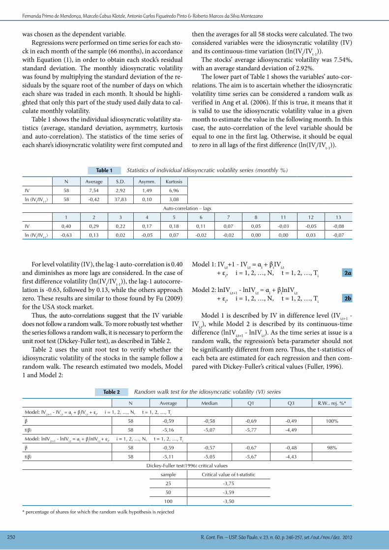
Table 1 shows the individual idiosyncratic volatility sta-tistics (average, standard deviation, asymmetry, kurtosis and auto-correlation). The statistics of the time series of each share’s idiosyncratic volatility were first computed and

then the averages for all 58 stocks were calculated. The two considered variables were the idiosyncratic volatility (IV) and its continuous-time variation (ln(IVt/IVt-1)).

The stocks’ average idiosyncratic volatility was 7.54%, with an average standard deviation of 2.92%.

The lower part of Table 1 shows the variables’ auto-cor-relations. The aim is to ascertain whether the idiosyncratic volatility time series can be considered a random walk as verified in Ang et al. (2006). If this is true, it means that it is valid to use the idiosyncratic volatility value in a given month to estimate the value in the following month. In this case, the auto-correlation of the level variable should be equal to one in the first lag. Otherwise, it should be equal to zero in all lags of the first difference (ln(IVt/IVt-1)).

Table 1 Statistics of individual idiosyncratic volatility series (monthly %)

N Average S.D. Asymm. Kurtosis

IV 58 7,54 2,92 1,49 6,96

ln (IVt/IVt-1) 58 -0,42 37,83 0,10 3,08

Auto-correlation – lags

1 2 3 4 5 6 7 8 11 12 13

IV 0,40 0,29 0,22 0,17 0,18 0,11 0,07 0,05 -0,03 -0,05 -0,08

ln (IVt/IVt-1) -0,63 0,13 0,02 -0,05 0,07 -0,02 -0,02 0,00 0,00 0,03 -0,07

For level volatility (IV), the lag-1 auto-correlation is 0.40 and diminishes as more lags are considered. In the case of first difference volatility (ln(IVt/IVt-1)), the lag-1 autocorre-lation is -0.63, followed by 0.13, while the others approach zero. These results are similar to those found by Fu (2009) for the USA stock market.

Thus, the auto-correlations suggest that the IV variable does not follow a random walk. To more robustly test whether the series follows a random walk, it is necessary to perform the unit root test (Dickey-Fuller test), as described in Table 2.

Table 2 uses the unit root test to verify whether the idiosyncratic volatility of the stocks in the sample follow a random walk. The research estimated two models, Model 1 and Model 2:

Model 1: IVi,t+1 - IVi,t = αi + βiIVi,t + εi, i = 1, 2, …, N, t = 1, 2, …, Ti 2a

Model 2: lnIVi,t+1 - lnIVi,t = αi + βilnIVi,t + εi, i = 1, 2, …, N, t = 1, 2, …, Ti 2b

Model 1 is described by IV in difference level (IVi,t+1 - IVi,t), while Model 2 is described by its continuous-time difference (lnIVi,t+1 - lnIVi,t). As the time series at issue is a random walk, the regression’s beta-parameter should not be significantly different from zero. Thus, the t-statistics of each beta are estimated for each regression and then com-pared with Dickey-Fuller’s critical values (Fuller, 1996).

Table 2 Random walk test for the idiosyncratic volatility (VI) series

N Average Median Q1 Q3 R.W.. rej. %*

Model: IVi,t+1 - IVi,t = αi + βiIVi,t + εi, i = 1, 2, …, N, t = 1, 2, …, Ti

β 58 -0,59 -0,58 -0,69 -0,49 100%

t(β) 58 -5,16 -5,07 -5,77 -4,49

Model: lnIVi,t+1 - lnIVi,t = αi + βilnIVi,t + εi, i = 1, 2, …, N, t = 1, 2, …, Ti

β 58 -0,59 -0,57 -0,67 -0,48 98%

t(β) 58 -5,11 -5,05 -5,67 -4,43

Dickey-Fuller test(1996) critical values

sample Critical value of t-statistic

25 -3,75

50 -3,59

100 -3,50

* percentage of shares for which the random walk hypothesis is rejected



Table 2 shows the averages and medians, as well as quar-tiles 1 and 3, of the beta obtained for each of the 58 stocks in the sample. The “R.W. rej. %” column shows the percen-tage of shares for which the random walk hypothesis was rejected in each model at a significance level of 1%: 100% in the first model and 98% in the second. This demonstra-tes that it is not appropriate to represent this variable as a random walk.

The next step is to analyze the Autoregressive Condi-tionally Heteroscedastic (ARCH) models that will also be used in the modeling of IV in this study. First of all, the-se models do not assume constant error variance; that is, they are heteroscedastic models. The second characteristic is related to the phenomenon known as volatility cluste-ring, which represents the tendency, in financial series, of large variations in asset prices (positive or negative) to be followed by large variations, and small variations in asset prices (positive or negative) to be followed by small varia-tions (Brooks, 2008). In other words, volatility tends to be auto-correlated to some extent.

These two characteristics are present in the ARCH mo-del because of the way conditional variance is modeled, where the error variance of the hypothetical regression is considered to be dependent on the lagged squared errors. The generalized ARCH (GARCH) model, developed by Bollerslev (1986), is an extension of the ARCH model. In the GARCH model, conditional variance may depend on its own lags in addition to lagged error, so the model allo-ws information on past squared errors to influence current variation without having to include multiple parameters. An example of the GARCH (p,q) model can be observed in Equation (3):

yt = β0 + β1 x1t + β2 x2t + ... + βn xnt + ut, ut ~ N(0,σt2)

σt2 = α0 + α1 ut-1

2 + α2 ut-22 + … + αq ut-q

2 + β1 σt-12

+ β2 σt-22+ ... + βp σt-p

2 3

where ut and σt2 are the regression’s errors and error varian-

ce, respectively. However, although widely used in financial series, the

model presented above is not without criticism. Parame-ter non-negativity conditions, in the case of conditional variance, may still not be observed, thus generating ne-gative variances. In addition, the model does not correct the so-called leverage effect that is very common in fi-nancial series. The leverage effect refers to the fact that negative shocks have a greater effect on volatility than positive shocks; that is, they generate a greater increase in volatility. According to the GARCH model, positive and negative shocks affect variance in the same way.

Finally, the exponential GARCH (EGARCH) model proposed by Nelson (1991), an extension of the GARCH model, should be highlighted. This model has a series of advantages, such as the impossibility of generating negative variances and permitting the existence of asymmetries in the model (leverage effect). The EGARCH (p,q) model, in general terms, can be written as follows:

yt = β0 + β1 x1t + β2 x2t + ... + βn xnt+ ut, ut ~ N(0,σt2)

ln(σt2)= ω + bl ln(σt-1

2)+ ck γ +α - 4

In Equation (4), because the logarithm of variance is specified, σt2 will be positive even if the model’s parameters are negative.

Due to its properties, which are perfectly suited to mo-deling volatility in financial series, the EGARCH model was used in this study as an alternative way of estimating idiosyncratic volatility. Because it provides a conditional variance series for each estimated model, the EGARCH model is useful as a way of estimating expected idiosyncra-tic volatility (Fu, 2009).

The second method used to calculate the idiosyncratic volatility of the shares in the sample was thus constituted by the EGARCH model described above. Fama and French’s (1993) Three-Factor Model was used once again, this time using monthly data. A regression was estimated for each stock, covering the entire sample period. Equation (5) was the regression used in this stage: Rit–rt=αi+bi(Rmt–rt)+siSMBt+hiHMLt+ uit, ut ~ N(0,σit

2)

ln(σit2)=ω+ bi,l ln(σi,t-1

2)+ ci,k γ +α - 5

The dependent variable (Rit – rt) is the excess monthly return of each stock, or its monthly return after deducting the Brazilian CDI rate. The Rmt – rt variable represents the excess market return. The monthly market return was cal-culated by weighting individual monthly returns according to each stock’s market value. The SMB and HML variables followed the same methodology described above. All re-turns were calculated continuously.

The regressions were performed using the EGARCH me-thod. Following Fu’s (2009) method, nine EGARCH(p,q) models were estimated for each stock: EGARCH(1,1), EGARCH(1,2), EGARCH(1,3), EGARCH(2,1), EGARCH(2,2), EGARCH(2,3), EGARCH(3,1), EGARCH(3,2) and EGARCH(3,3). Among the models that converged, the one with the lowest Akaike (AIC) criterion was selected for each stock.

In the sample of shares used in this study, EGARCH (2,2), which was selected for 13 of the 58 stocks, was the most common model, followed by EGARCH(3,1), which was used in 10 cases.

Finally, the individual conditional variance series were obtained according to the adopted model. The square root was removed from the obtained values to make them equi-valent to the idiosyncratic volatility values calculated using the first method (standard deviation of the monthly regres-sion residuals, according to the Fama and French model). Thus, the new time series correspond to each stock’s ex-pected idiosyncratic volatility. This new variable was called E(IV).

E(IV)’s descriptive statistics, as well as its respective continuous time variables (ln (E(IV)t/E(IV)t-1), are presen-ted in Table 3. As in the case of Table 1, the average, stan-dard deviation, asymmetry and kurtosis were computed for each of the 58 stocks in the sample and then the average

Σl=1

pΣk=1

q ut -k

σ2t-kσ2t-k

|ut -k| 2π

Σl=1

pΣk=1

q ui,t -k

σ2i,t-kσ2i,t-k

|ui,t -k| 2π



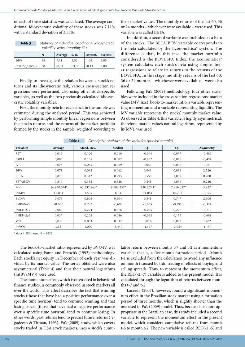
of each of these statistics was calculated. The average con-ditional idiosyncratic volatility of these stocks was 7.11% with a standard deviation of 3.53%.

Finally, to investigate the relation between a stock’s re-turns and its idiosyncratic risk, various cross-section re-gressions were performed, also using other stock-specific variables, as well as the two previously calculated idiosyn-cratic volatility variables.

First, the monthly beta for each stock in the sample was estimated during the analyzed period. This was achieved by performing simple monthly linear regressions between the stock’s returns and the returns of the market portfolio formed by the stocks in the sample, weighted according to

Table 3 Statistics of individual conditional idiosyncratic volatility series (monthly %)

N Average S. D. Asymm. Kurtosis

E(IV) 58 7,11 3,53 1,08 5,05

ln (E(IV)t/E(IV)t-1) 58 -0,11 63,98 -0,13 3,00

their market values. The monthly returns of the last 60, 36 or 24 months – whichever were available – were used. This variable was called BETA.

In addition, a second variable was included as a beta of the stocks. The BETAIBOV variable corresponds to the beta calculated by the Economática® system. The difference is that, in this case, the market portfolio considered is the BOVESPA Index: the Economática® system calculates each stock’s beta using simple line-ar regressions to relate its returns to the returns of the BOVESPA. In this stage, monthly returns of the last 60, 36 or 24 months – whichever were available – were also used.

Following Fu’s (2009) methodology, four other varia-bles were included in the cross-section regressions: market value (MV, size), book-to-market ratio, a variable represen-ting momentum and a variable representing liquidity. The MV variable represents the stocks’ monthly market value. As observed in Table 4, this variable is highly asymmetrical; therefore, market value’s natural logarithm, represented by ln(MV), was used.

Table 4 Descriptive statistics of the variables (pooled sample)

Variables Average Stand. Dev. Median Q1 Q3 Asymmetry

RET 0,015 0,106 0,016 -0,044 0,077 -0,482

EXRET 0,005 0,105 0,007 -0,052 0,066 -0,494

IV 0,075 0,035 0,069 0,053 0,090 1,961

E(IV) 0,071 0,043 0,062 0,043 0,088 2,526

BETA 0,810 0,342 0,795 0,555 1,059 0,200

BETAIBOV 0,819 0,335 0,826 0,548 1,034 0,236

MV 26.940.074* 62.232.263* 9.188.237* 2.825.241* 17.916.057* 3,927

ln(MV) 15,854 1,595 16,033 14,854 16,701 -0,127

BV/MV 0,679 0,608 0,504 0,348 0,747 2,608

ln(BV/MV) -0,687 0,792 -0,686 -1,055 -0,291 -0,374

lnRET(-2,-7) 0,060 0,274 0,076 -0,075 0,227 -0,710

lnRET(-2;-5) 0,037 0,203 0,046 -0,063 0,159 -0,681

VOL 0,039 0,033 0,032 0,016 0,052 1,782

ln(VOL) -3,651 1,070 -3,449 -4,127 -2,954 -1,150

* data in R$ thous. N = 3828

The book-to-market ratio, represented by BV/MV, was calculated using Fama and French’s (1992) methodology. Each stock’s net equity in December of each year was di-vided by its market value. The series obtained were also asymmetrical (Table 4) and thus their natural logarithms (ln(BV/MV)) were used.

The momentum effect, which is often cited in behavioral finance studies, is commonly observed in stock markets all over the world. This effect describes the fact that winning stocks (those that have had a positive performance over a specific time horizon) tend to continue winning and that losing stocks (those that have had a negative performance over a specific time horizon) tend to continue losing. In other words, past returns tend to predict future returns (Je-gadeesh & Titman, 1993). Fu’s (2009) study, which covers stocks traded in USA stock markets, uses a stock’s cumu-

lative return between months t-7 and t-2 as a momentum variable; that is, a five-month formation period. Month t-1 is excluded from the calculation to avoid any influence on month t caused by thin trading or effects of buying and selling spreads. Thus, to represent the momentum effect, the RET(-2;-7) variable is added to the present model. It is calculated through the logarithm of returns between mon-ths t-7 and t-2.

Lacerda (2007), however, found a significant momen-tum effect in the Brazilian stock market using a formation period of three months, which is slightly shorter than the one used in Fu’s (2009) model. Thus, because it is more ap-propriate in the Brazilian case, this study included a second variable to represent the momentum effect in the present model, which considers cumulative returns from month t-5 to month t-2. The new variable is called RET(-2;-5) and



is also calculated through the natural logarithm of returns. As a liquidity variable, the study used a turnover rate

constituted by the ratio between the average monthly tra-ded volume and the average market value of each stock during the preceding six months. This variable was called VOL. Additionally, the high asymmetry of the series, as observed in Table 4, led to the adoption of their natural logarithms (ln(VOL)).

To conclude, the RET variable represents the natural

logarithm of each stock’s monthly returns (continuous re-turns) and EXRET represents excess returns; that is, mon-thly returns after deducting the risk-free rate (CDI), also calculated continuously. All variables are presented in Table 4, along with their respective descriptive statistics (average, standard deviation, mean, the first and third quartiles and asymmetry). N represents the number of observations in each variable (stock-month). All statistics were calculated using pooled stock samples.

4 ReSuLTS

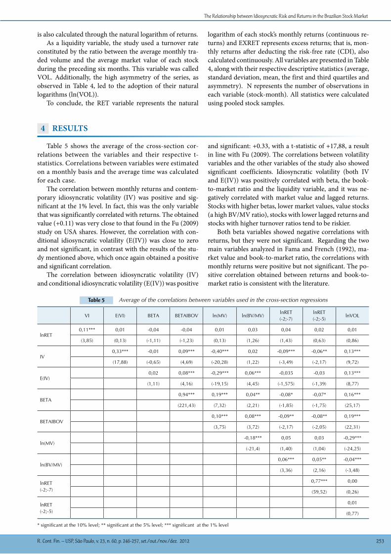
Table 5 shows the average of the cross-section cor-relations between the variables and their respective t-statistics. Correlations between variables were estimated on a monthly basis and the average time was calculated for each case.

The correlation between monthly returns and contem-porary idiosyncratic volatility (IV) was positive and sig-nificant at the 1% level. In fact, this was the only variable that was significantly correlated with returns. The obtained value (+0.11) was very close to that found in the Fu (2009) study on USA shares. However, the correlation with con-ditional idiosyncratic volatility (E(IV)) was close to zero and not significant, in contrast with the results of the stu-dy mentioned above, which once again obtained a positive and significant correlation.

The correlation between idiosyncratic volatility (IV) and conditional idiosyncratic volatility (E(IV)) was positive

and significant: +0.33, with a t-statistic of +17,88, a result in line with Fu (2009). The correlations between volatility variables and the other variables of the study also showed significant coefficients. Idiosyncratic volatility (both IV and E(IV)) was positively correlated with beta, the book-to-market ratio and the liquidity variable, and it was ne-gatively correlated with market value and lagged returns. Stocks with higher betas, lower market values, value stocks (a high BV/MV ratio), stocks with lower lagged returns and stocks with higher turnover ratios tend to be riskier.

Both beta variables showed negative correlations with returns, but they were not significant. Regarding the two main variables analyzed in Fama and French (1992), ma-rket value and book-to-market ratio, the correlations with monthly returns were positive but not significant. The po-sitive correlation obtained between returns and book-to-market ratio is consistent with the literature.

Table 5 Average of the correlations between variables used in the cross-section regressions

VI E(VI) BETA BETAIBOV ln(MV) ln(BV/MV)lnRET (-2;-7)

lnRET (-2;-5)

lnVOL

lnRET0,11*** 0,01 -0,04 -0,04 0,01 0,03 0,04 0,02 0,01

(3,85) (0,13) (-1,11) (-1,23) (0,13) (1,26) (1,43) (0,63) (0,86)

IV0,33*** -0,01 0,09*** -0,40*** 0,02 -0,09*** -0,06** 0,13***

(17,88) (-0,65) (4,69) (-20,28) (1,22) (-3,49) (-2,17) (9,72)

E(IV)0,02 0,08*** -0,29*** 0,06*** -0,035 -0,03 0,13***

(1,11) (4,16) (-19,15) (4,45) (-1,575) (-1,39) (8,77)

BETA0,94*** 0,19*** 0,04** -0,08* -0,07* 0,16***

(221,43) (7,32) (2,21) (-1,85) (-1,75) (25,17)

BETAIBOV0,10*** 0,08*** -0,09** -0,08** 0,19***

(3,75) (3,72) (-2,17) (-2,05) (22,31)

ln(MV)-0,18*** 0,05 0,03 -0,29***

(-21,4) (1,40) (1,04) (-24,25)

ln(BV/MV)0,06*** 0,05** -0,04***

(3,36) (2,16) (-3,48)

lnRET (-2;-7)

0,77*** 0,00

(59,52) (0,26)

lnRET (-2;-5)

0,01

(0,77)

* significant at the 10% level; ** significant at the 5% level; *** significant at the 1% level



With regard to the momentum variables, both were positively (though not significantly) correlated with re-turns, which can be explained by behavioral finance the-ory. However, one may observe that the t-statistic related to RET (-2;-7) (+1.43) was much higher than that of the second momentum variable (+0.63), and the obtained correlation value (+0.04) was double that of the second case (+0.02). These results may be taken as evidence that the periods during which the momentum effect is stron-ger in Brazil are aligning more with those verified in the USA stock market.

The result of the liquidity variable, represented by ln-VOL, diverged from that found in the literature when its correlation with returns was analyzed. Studies show that less liquid stocks tend to provide greater returns. The result showed a slightly positive correlation between returns and the liquidity index but the t-statistic was not significant at the 10% level.

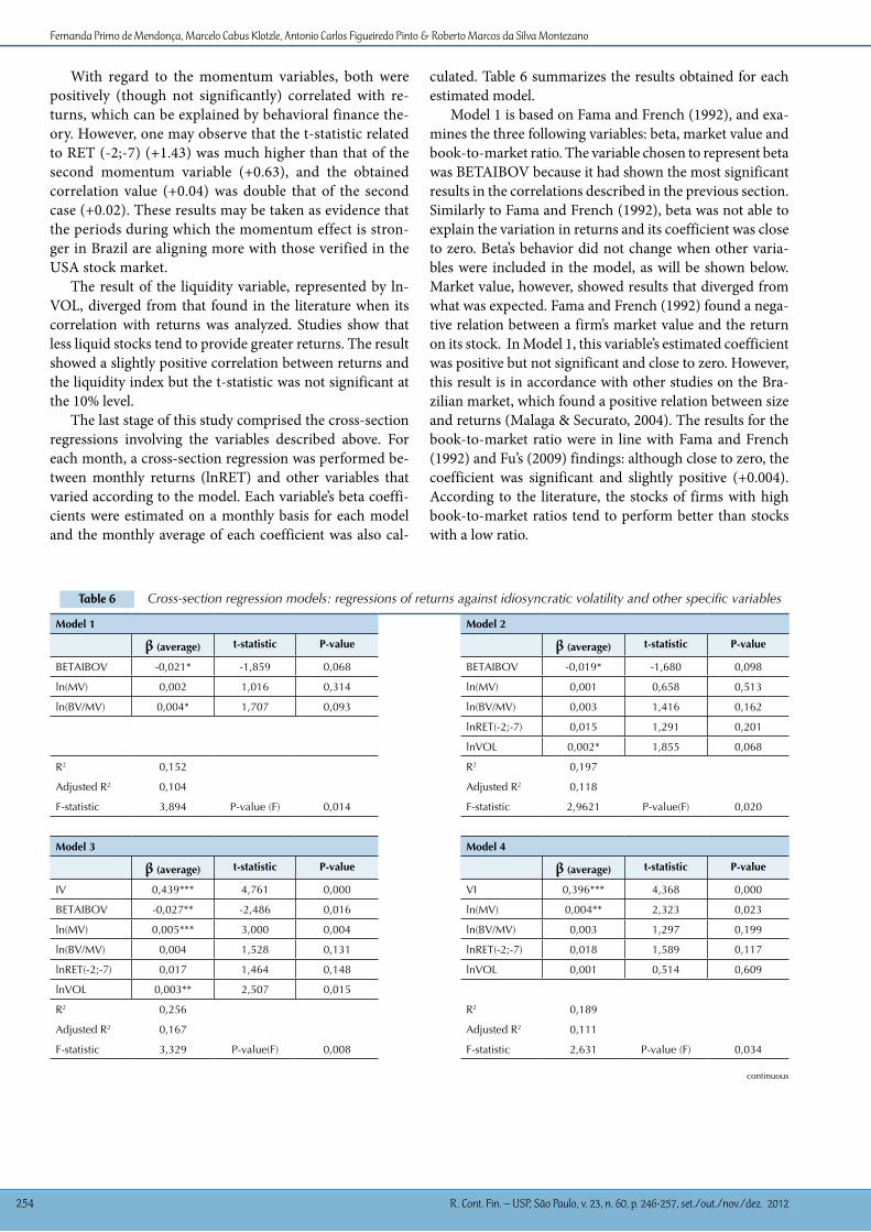
The last stage of this study comprised the cross-section regressions involving the variables described above. For each month, a cross-section regression was performed be-tween monthly returns (lnRET) and other variables that varied according to the model. Each variable’s beta coeffi-cients were estimated on a monthly basis for each model and the monthly average of each coefficient was also cal-

culated. Table 6 summarizes the results obtained for each estimated model.

Model 1 is based on Fama and French (1992), and exa-mines the three following variables: beta, market value and book-to-market ratio. The variable chosen to represent beta was BETAIBOV because it had shown the most significant results in the correlations described in the previous section. Similarly to Fama and French (1992), beta was not able to explain the variation in returns and its coefficient was close to zero. Beta’s behavior did not change when other varia-bles were included in the model, as will be shown below. Market value, however, showed results that diverged from what was expected. Fama and French (1992) found a nega-tive relation between a firm’s market value and the return on its stock. In Model 1, this variable’s estimated coefficient was positive but not significant and close to zero. However, this result is in accordance with other studies on the Bra-zilian market, which found a positive relation between size and returns (Malaga & Securato, 2004). The results for the book-to-market ratio were in line with Fama and French (1992) and Fu’s (2009) findings: although close to zero, the coefficient was significant and slightly positive (+0.004). According to the literature, the stocks of firms with high book-to-market ratios tend to perform better than stocks with a low ratio.

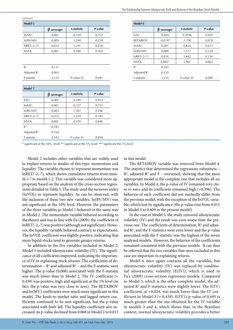
Table 6 Cross-section regression models: regressions of returns against idiosyncratic volatility and other specific variables

Model 1 Model 2

β (average) t-statistic P-value β (average) t-statistic P-value

BETAIBOV -0,021* -1,859 0,068 BETAIBOV -0,019* -1,680 0,098

ln(MV) 0,002 1,016 0,314 ln(MV) 0,001 0,658 0,513

ln(BV/MV) 0,004* 1,707 0,093 ln(BV/MV) 0,003 1,416 0,162

lnRET(-2;-7) 0,015 1,291 0,201

lnVOL 0,002* 1,855 0,068

R2 0,152 R2 0,197

Adjusted R2 0,104 Adjusted R2 0,118

F-statistic 3,894 P-value (F) 0,014 F-statistic 2,9621 P-value(F) 0,020

Model 3 Model 4


IV 0,439*** 4,761 0,000 VI 0,396*** 4,368 0,000

BETAIBOV -0,027** -2,486 0,016 ln(MV) 0,004** 2,323 0,023

ln(MV) 0,005*** 3,000 0,004 ln(BV/MV) 0,003 1,297 0,199

ln(BV/MV) 0,004 1,528 0,131 lnRET(-2;-7) 0,018 1,589 0,117

lnRET(-2;-7) 0,017 1,464 0,148 lnVOL 0,001 0,514 0,609

lnVOL 0,003** 2,507 0,015

R2 0,256 R2 0,189


F-statistic 3,329 P-value(F) 0,008 F-statistic 2,631 P-value (F) 0,034

continuous



Model 5 Model 6


ln(MV) 0,001 0,318 0,752 E(IV) 0,024 0,3936 0,695

ln(BV/MV) 0,003 1,240 0,219 BETAIBOV -0,019* -1,790 0,078

lnRET(-2;-7) 0,014 1,191 0,238 ln(MV) 0,001 0,824 0,413

lnVOL 0,001 0,580 0,564 ln(BV/MV) 0,004 1,517 0,134

lnRET(-2;-7) 0,016 1,442 0,154

lnVOL 0,002* 1,901 0,062

R2 0,131 R2 0,243


F-statistic 2,123 P-value (F) 0,091 F-statistic 3,235 P-value (F) 0,009

Model 7

β (average) t-statistic P-value

E(IV) 0,007 0,109 0,913

ln(MV) 0,001 0,337 0,737

ln(BV/MV) 0,003 1,307 0,196

lnRET(-2;-7) 0,015 1,339 0,185

lnVOL 0,001 0,470 0,640

R2 0,183

Adjusted R2 0,104

F-statistic 2,553 P-value (F) 0,039

* significant at the 10% level; ** significant at the 5% level; *** significant the 1% level

continued

Model 2 includes other variables that are widely used to explain returns in studies of this type: momentum and liquidity. The variable chosen to represent momentum was lnRET(-2;-7), which shows cumulative returns from mon-th t-7 to month t-2. This variable was considered more ap-propriate based on the analysis of the cross-section regres-sions detailed in Table 5. The study used the turnover index (lnVOL) to represent liquidity. As can be observed, with the inclusion of these two new variables, ln(BV/MV) was not significant at the 10% level. However, the parameters of the three variables in Model 1 behaved in the same way in Model 2. The momentum variable behaved according to the theory and was in line with Fu (2009): the coefficient of lnRET(-2;-7) was positive (although not significant). Howe-ver, the liquidity variable behaved contrary to expectations. The lnVOL coefficient was slightly positive, indicating that more liquid stocks tend to generate greater returns.

In addition to the five variables included in Model 2, Model 3 included idiosyncratic volatility (IV). The signifi-cance of all coefficients improved, indicating the importan-ce of IV in explaining stock returns. The coefficients of de-termination – R2 and adjusted R2 – and the F-statistic were higher. The p-value (0,008) associated with the F-statistic was much lower than in Model 2. The IV coefficient (+ 0.439) was positive, high and significant at the 1% level (in fact, the p-value was very close to zero). The BETAIBOV and ln(MV) coefficients were much more significant in this model. The book-to-market ratio and lagged return coe-fficients continued to be non-significant, but the p-value associated with both fell. The liquidity coefficient also in-creased: its p-value declined from 0.068 in Model 2 to 0.015

in this model. The BETAIBOV variable was removed from Model 4.

The statistics that determined the regressions robustness – R2, adjusted R2 and F – worsened, showing that the most appropriate model is the complete one that includes all six variables. In Model 4, the p-value of IV remained very clo-se to zero, and its coefficient remained high (+0.396). The behavior of each coefficient did not markedly differ from the previous model, with the exception of the InVOL varia-ble, which lost its significance (the p-value rose from 0.015 in Model 3 to 0.609 in the present model).

In the case of Model 5, the study removed idiosyncratic volatility (IV) and the result was even worse than the pre-vious one. The coefficients of determination, R2 and adjus-ted R2, and the F-statistics were even lower and the p-value associated with the F-statistic was the highest of the seven analyzed models. However, the behavior of the coefficients remained consistent with the previous models. It can thus be inferred that the two variables that were excluded in this case are important in explaining returns.

Model 6 once again contains all the variables, but idiosyncratic volatility (IV) was replaced by conditio-nal idiosyncratic volatility (E(IV)), which is used in Fu’s (2009) cross-section regression models. Compared to Model 3, which is the other complete model, the ad-justed R2 and F-statistics were slightly lower. The E(IV) coefficient, at +0,024, was much lower than the IV coe-fficient in Model 3 (+ 0.439). E(IV)’s p-value of 0.695 is much greater than the one obtained for the IV variable in models 3 and 4, which shows that, in the Brazilian context, normal idiosyncratic volatility provides a better



explanation for returns. In Fu (2009), both normal and conditional idiosyncratic volatility are significant as ex-planatory variables for returns.

Removing the BETAIBOV variable from Model 7 did not improve the regressions’ significance levels. All coefficients lost significance. E(IV)’s p-value rose even more to 0.913.

Some inferences can be made from the results of these seven models. The value of beta was close to zero, as expected. The results for market value were the op-posite of those found in USA studies but consistent with the findings of Brazilian studies. Its coefficient was slightly positive in all models indicating that, in the Brazilian context and in the considered sample, lar-ger firms have slightly larger returns. The liquidity va-riable results were contrary to expectations. According to the literature, less liquid stocks tend to have higher returns. In all the studied models, however, the InVOL parameter was slightly positive. The book-to-market ratio and lagged returns behaved as expected. Value stocks and stocks with a good past performance tend to achieve higher returns.

The study’s main finding was that idiosyncratic vola-

tility was significant in explaining stock returns. The co-efficients of IV in the regressions in which this variable was included, Models 3 and 4, were +0.439 and + 0.396, respectively, and both were significant at the 1% level. As can be observed, they constitute the models’ largest co-efficients, showing that IV, amongst those analyzed, was the factor that most influenced stock returns. IV’s inclu-sion in the model increased its explanatory power: the adjusted R2 coefficient increased from 11.8% in Model 2 to 16.7% in Model 3, while the p-value of the f-statistic fell from 2.0% to 0.8%.

Conditional idiosyncratic volatility, however, did not perform as well and, although it is usually an efficient me-asure of expected idiosyncratic volatility, it is not as appro-priate for the considered sample and period as IV. In the models that included E(IV), (Models 6 and 7), this variable was not significant. The statistics that indicate the model’s quality were slightly worse than in the models with IV (Models 3 and 4).

The most appropriate model was the third one, which includes all the explanatory variables (BETAIBOV, ln(MV), ln(BV/MV), lnRET(-2;-7) e lnVOL), as well as idiosyncra-tic volatility (IV).

5 ConCLuSIon

This study sought to relate the idiosyncratic risk of sto-cks traded in the Brazilian stock market to their returns. Idiosyncratic volatility and conditional idiosyncratic vola-tility were estimated for each stock in the sample during the period from July 2005 to December 2010, following Fu’s (2009) methodology.

Cross-section regression models were constructed to verify this relationship. Based on an examination of the financial asset-pricing literature, a series of characteristic stock-related variables were selected and added to the re-gressions: market value, book-to-market ratio, beta, the momentum effect and liquidity. The inclusion of these variables aimed to analyze their influence on returns and verify whether their behavior was in accordance with the literature’s findings. In addition, it was possible to analyze the effect of idiosyncratic volatility in models that included these types of variables.

The two estimated idiosyncratic volatility variables – idiosyncratic volatility and conditional idiosyncratic vola-tility – were analyzed in separate models. The results ob-tained by the analysis of the correlations of the variables and the statistics of the estimated models showed that idio-syncratic volatility (IV) was an excellent explanatory fac-

tor for returns, whereas conditional idiosyncratic volatility (E(IV)) was, as expected, unable to explain returns.

The analysis of the other variables also produced impor-tant results. Contrary to expectations, stock market value and liquidity had an important influence on returns. The-se variables’ coefficients were positive in all the analyzed models. This result may reflect the particularities of the Brazilian market, which is smaller, more recent and less consolidated than the USA stock market.

However, the results relating to the book-to-market ratio and the momentum effect were consistent with the literature. Value stocks and those with a good past perfor-mance tended to produce higher returns.

The most appropriate of the analyzed models was the one that included all the employed variables. The statistics and significance of the variables’ coefficients showed the best results in Model three, which included normal idio-syncratic volatility and the other five selected variables.

It should be highlighted that studies of this type that fo-cus on the Brazilian market are still scarce. However, more complete studies can be performed with this methodology, using a bigger sample, covering a greater period of time or including new variables in the models.

Ang, A., Hodrick, R. J., Xing, Y., & Zhang, X. (2006). The cross-section of volatility and expected returns. Journal of Finance, 61 (1), 259-299.

Ang, A., Hodrick, R. J., Xing, Y., & Zhang, X. (2009). High idiosyncratic volatility and low returns: international and further U.S. evidence. Journal of Financial Economics, 91 (1), 1-23.

Angelidis, T. (2010). Idiosyncratic risk in emerging markets. Financial

Review, 45 (4), 1053-1078.Bali, T. G., & Cakici, N. (2006). Aggregate idiosyncratic risk and market

returns. Journal of Investment Management, 4 (4), 4-14. Banz, R. W. (1981). The relationship between return and market value of

common stocks. Journal of Financial Economics, 9 (1), 3-18. Bollerslev, T. (1986). Generalized autoregressive condicional

References



heteroskedasticity. Journal of Econometrics, 31 (3), 307-327. Brooks, C. (2008). Introductory econometrics for finance. 2. ed. Cambridge,

U.K.: Cambridge University Press. Campbell, J. Y. L., Martin, M., Burton G., & Xu, Y. (2001). Have

individual stocks become more volatile? An empirical exploration of idiosyncratic risk. Journal of Finance, 56 (1), 1-43.

Comdinheiro (2012). Retrieved from http://www.comdinheiro.com.br/Risco#.

Costa Jr., N., & Neves, M. B. E. (2000). Variáveis fundamentalistas e os retornos das ações. Revista Brasileira de Economia, 54 (1), 123-137.

Estrada, J. (2002). Systematic risk in emerging markets: the D-CAPM. Emerging Markets Review, 3 (4), 365-379.

Fama, E., & French, K. (1992). The cross-section of expected stock returns. Journal of Finance, 47 (2), 427-465.

Fama, E., & French, K. (1993). Common risk factors in the returns on stocks and bonds. Journal of Financial Economics, 33 (1), 3-56.

Fama, E., & Macbeth, J. D. (1973). Risk, return and equilibrium: empirical tests. Journal of Political Economy, 81 (3), 607-636.

Fu, F. (2009). Idiosyncratic risk and the cross-section of expected stock returns. Journal of Financial Economics, 91 (1), 24-37.

Fu, F., & Schutte, M. G. (2010). Investor diversification and the pricing of idiosyncratic risk. Proceedings from the 2010 FMA Asian Conference. Singapore.

Fuller, W. (1996). Introduction to statistical time series. New York: Wiley. Galdi, F. C., & Securato, J. R. (2007). O risco idiossincrático é relevante no

mercado brasileiro? Revista Brasileira de Finanças, 5 (1), 41-58. Goyal, A., & Santa-Clara, P. (2003). Idiosyncratic risk matters! Journal of

Finance, 58 (3), 975-1007. Huang, W., Liu, Q., Rhee, S. G., & Zhang, L. (2010). Return reversals,

idiosyncratic risk and expected returns. Review of Financial Studies, 23 (1), 147-168.

Jegadeesh, N., & Titman, S. (1993). Returns to buying winners and selling losers: implications for stock market efficiency. Journal of Finance, 48 (1), 65-92.

Kearney, C., & Poti, V. (2008). Have European stocks become more volatile? An empirical investigation of idiosyncratic and market risk in the Euro area. European Financial Management, 14 (3), 419-444.

Kotiaho, H. (2010). Idiosyncratic risk, financial distress and the cross-section of stock returns. Finance Master's thesis, Helsinki School of Economics,

Department of Accounting and Finance, Helsinki, Finnland.Lacerda, R. T. (2007). Estratégias de investimento para o Brasil baseadas

em finanças comportamentais. Tese (Finance Master's thesis), Escola de Pós-Graduação em Economia (EPGE), Fundação Getúlio Vargas, Rio de Janeiro, Brasil.

Levy, H. (1978). Equilibrium in an imperfect market: a constraint on the number of securities in the portfolio. American Economic Review, 68 (4), 643-658.

Lintner, J. (1965). The valuation of risk assets and the selection of risky investments in stock portfolios and capital budgets. Review of Economics and Statistics, 47 (1), 13-37.

Malaga, F., & Securato, J. R. (2004). Aplicação do modelo de três fatores de Fama e French no mercado acionário brasileiro - um estudo empírico no período 1995-2003. Anais do Encontro Nacional da Associação Nacional de Pós-Graduação e Pesquisa em Administração (ENANPAD), Curitiba, PR, Brasil, 28.

Malkiel, B. G., & Xu, Y. (2002). Idiosyncratic risk and security returns. University of Texas at Dallas, Unpublished, mimeo.

Martin, D. M. L., Cia, J. C., & Kayo, E. K. (2010). Determinantes do risco idiossincrático no Brasil no período de 1996 a 2009. Anais do Encontro Nacional da Associação Nacional de Pós-Graduação e Pesquisa em Administração (ENANPAD), Rio de Janeiro, RJ, Brasil, 34.

Merton, R. (1973). A simple model of capital market equilibrium with incomplete information. Journal of Finance, 42 (3), 483-510.

Nelson, D. B. (1991). Conditional heteroskedasticity in asset returns: a new approach. Econometrica, 59 (2), 347-370.

Ricca, B. O. G. (2010). Apreçamento da assimetria idiosincrática no mercado de ações brasileiro. Dissertação de mestrado, Escola de Pós-Graduação em Economia da Fundação Getúlio Vargas, Rio de Janeiro, Brasil.

Rogers, P., & Securato, J. R. (2009). Estudo comparativo no mercado brasileiro do Capital Asset Pricing Model (CAPM), Modelo 3-Fatores de Fama e French e Reward Beta Approach. RAC-Eletrônica, 3 (1), 159-179.

Sharpe, W. F. (1964). Capital asset prices: a theory of market equilibrium under conditions of risk. Journal of Finance, 19 (3), 425-442.

Stattman, D. (1980). Book values and stock returns. The Chicago MBA: A Journal of Selected Papers, 4, 25-45.

the relationship between idiosyncratic risk and · pdf filethe relationship between...

Documents