Financial Distress and Corporate Risk Management:

Theory & Evidence

Amiyatosh Purnanandam∗

(Job Market Paper)

First Draft : August, 2003

This Draft : January, 2004

∗401 Sage Hall, Johnson Graduate School of Management, Cornell University, Ithaca, NY - 14853. email:

akp22@cornell.edu. I would like to thank Warren Bailey, Sudheer Chava, Thomas Chemmanur, John Gra-

ham, Robert Goldstein, Yaniv Grinstein, Jerry Haas, Pankaj Jain, Robert Jarrow, Kose John, Haitao Li,

Roni Michaely, Maureen O’Hara, Mitch Petersen, Bhaskaran Swaminathan, David Weinbaum and semi-

nar participants at Cornell University and Lehman Brothers Finance Fellowship Competition for valuable

comments and suggestions. All remaining errors are mine.

1

Abstract

This paper develops a theory of corporate risk-management in the presence of deadweightlosses caused by financial distress and tests its implications using a comprehensive datasetof over 3000 non-financial firms. Unlike extant theories that explain only the ex-ante risk-management behavior of a firm, I show that the shareholders optimally engage in ex-postrisk-management activities even without a pre-commitment to do so. I generate new cross-sectional predictions by relating firm characteristics such as leverage and deadweight lossesfrom financial distress to its risk-management incentives. The model predicts a positive re-lationship between leverage and hedging for moderately leveraged firms. This relationshipreverses, however, for highly leveraged firms. Similarly the model produces a non-monotonicrelationship between leverage and hedging for high market-to-book value firms. The em-pirical findings are consistent with these predictions. The empirical study presents the firstlarge-sample evidence on the extent of hedging by non-financial firms and provides many newfindings. I find that large and small firms hedge for different reasons. While both groupshedge in response to the financial distress costs and exhibit economies of scale in hedging,large firms also hedge in response to underinvestment costs and tax-convexity, as predictedby the existing theories.

2

1 Introduction

This paper develops and tests a theory of corporate risk-management in the presence of

deadweight losses caused by financial distress. The existing literature shows that hedging

can lead to firm value maximization by limiting deadweight losses of bankruptcy (see Smith

and Stulz (1985)).1 These models justify only ex-ante2 risk-management behavior on the

part of the firm. Ex-post, shareholders of a levered firm may not find it optimal to engage

in hedging activities due to their risk-shifting incentives (Jensen and Meckling (1976)). I

extend the current literature by explaining the ex-post risk-management motivation of the

firm. The model generates new cross-sectional predictions by relating firm characteristics

such as leverage, deadweight losses and project maturity to risk-management incentives.

I test these predictions with hedging data of COMPUSTAT-CRSP firms, meeting some

reasonable sample selection criteria, for fiscal years 1996-97. The empirical study presents

the first large sample evidence on the determinants of firms’ hedging activities3 and provides

new findings.

The key assumption underlying my theory is the distinction between ‘financial distress’

and ‘insolvency’. I assume that apart from the ‘solvent’ and the ‘insolvent’ states, a firm

faces an intermediate state called ‘financial distress’. ‘Financial Distress’ is defined as a low

cash-flow state of the firm in which it incurs deadweight losses without being insolvent. The

notion that financial distress is a different state from insolvency has some precedence in the

literature. Titman (1984) uses a similar assumption to study the effect of capital structure

on a firm’s liquidation decisions. The idea of a financially distressed firm in my model is

consistent with the notion of an illiquid but solvent firm in Diamond (1991) or a firm with

low cash-flow in Froot, Scharfstein and Stein (1993).

1Other motivations for corporate hedging include convexity of taxes, managerial risk-aversion(Stulz (1984), Smith and Stulz (1985)), underinvestment costs (Froot, Scharfstein and Stein (1993))and information asymmetry between the managers and outsiders of the firm (DeMarzo and Duffie(1991,1995)).

2Throughout the paper, I use the terms ’ex ante’ and ’ex post’ with respect to the time ofborrowing.

3Due to data limitations, the earlier studies have used small samples to investigate the determi-nants of firms’ hedging activities (see Nance, Smith and Smithson (1993), Tufano (1996), Geczy,Minton and Schrand (1997), Haushalter (2000) and Graham and Rogers (2002)). Mian (1996)provides large-sample evidence on the yes-no decision of hedging. In contrast, I use data on theextent of hedging as well and provide many new findings.

3

There are three important sources of deadweight losses from financial distress. First, a

financially distressed firm may lose customers, valuable suppliers and key employees.4 Opler

and Titman (1994) provide empirical evidence that financially distressed firms lose significant

market share to their healthy counterparts in industry downturns. Secondly, a financially

distressed firm is more likely to violate its debt covenants5 or miss coupon/principal payments

without being insolvent.6 These violations impose deadweight losses in the form of financial

penalties, accelerated debt-repayment, operational inflexibility and managerial time and

resources spent on negotiations with the lenders. For example, when Delta airlines violated

a debt-to-equity ratio covenant in 2002, it was required by its lenders to maintain a minimum

of $1 billion in cash and cash equivalents at the end of every month from October 2002 until

June 2003.7 Finally, a financially distressed firm may have to forego positive NPV projects

due to costly external financing, as in Froot et al. (1993).

I develop a dynamic model of a firm that issues equity capital and zero coupon bonds

to invest in a risky asset. The firm makes an initial investment with the consent of its

bondholders. At a later date, shareholders can modify the firm’s investment risk by replacing

the existing asset with a new one or by entering into derivatives transactions. The asset value

evolves according to a stochastic process. The firm is in financial distress if the asset value

falls below some lower threshold during its life. In this state, the firm is unable to realize its

full upside potential due to lost real options, loss of customers and suppliers or losses imposed

by its bondholders. Insolvency occurs on the maturity date if terminal asset value is below

the face value of debt and, consequently, debtholders gain control of the firm. Shareholders’

4For example, in the mid-1990s Apple Computers had financial difficulties leading to speculationsabout its long-term survival (see Business Week, January, 29 and February 5, 1996). Softwaredevelopers were reluctant to develop new application software for the Mac-users, which was partlyresponsible for a decline of 27% in the unit sales of Mac computers from 1996 to 1997 (see Apple’s1998 10-K filings with the SEC). Similarly, when Chrysler faced financial difficulties in the early1980s, Lee Iacocca (former CEO of the company) observed that "its share of new car sales droppednearly two percentage points because potential buyers feared the company would go bankrupt"(quoted from Titman (1984)).

5Lenders often impose debt-covenants such as maintenance of minimum net-worth or maximumdebt-to-equity ratio by the borrowing firms. See Smith and Warner (1979), Kalay (1982) andDichev and Skinner (2001).

6Moody’s Investor Service Report (1998) shows that during 1982-1997 about 50% of the long-term publicly traded bond defaults (including missed or delayed payment of coupon and principal)didn’t result in bankruptcy filings.

7See Delta’s 2002 10-K filings with the SEC.

4

final payoffs depend on the terminal asset value as well as on the path taken by the firm’s

asset8 over its life.

The optimal level of ex-post investment risk, from the shareholders’ perspective, is deter-

mined by a trade-off between deadweight losses from financial distress and value associated

with the limited liability of the firm’s equity.9 Unlike the risk-shifting models such as Jensen

and Meckling (1976), equity-value is not always an increasing function of firm risk in my

model. While a high risk project increases the value of equity’s limited liability, it also im-

poses a cost on the shareholders by increasing the expected cost of financial distress. Due to

these losses, the shareholders find it optimal to implement a risk-management strategy ex-

post even in the absence of an explicit pre-commitment to do so.10 If losses in the products

market (such as lost customers and suppliers) or losses due to suboptimal investment strat-

egy are large, shareholders engage in risk-management strategy even without debt-covenants.

Otherwise, in a rational expectation framework, the bondholders can set these covenants ex-

ante such that shareholders implement a desired risk-management strategy ex-post.

The optimal investment risk in my model depends on firm leverage, the financial distress

boundary, the time horizon of the project and deadweight losses incurred in financial distress.

As in the extant models (Smith and Stulz (1985)), I show that a firm with high leverage (fi-

nancial distress) has a higher incentive to engage in hedging activities. However, by explicitly

modelling the shareholders’ risk-shifting incentives, my model shows that risk-management

incentives disappear for firms with extremely high leverage. Similarly, the relationship be-

tween leverage and hedging is predicted to be non-monotonic for a firm with high deadweight

losses from financial distress (such as a high market-to-book value firm). The model shows

8This approach is similar to valuation of equity as a path-dependent (down-and-out call) option.The equity value in my model differs from the corresponding barrier option by the amount ofdeadweight losses incurred in financial distress. Brockman and Turtle (2003) provide some empiricalevidence in support of equity’s valuation as a path-dependent option.

9In the context of swap markets, Mozumdar (2000) demonstrates the trade-off between risk-shifting and hedging incentives in the presence of information asymmetry about the firm type. Hismodel relates hedging incentives to firm type.10Other papers analyzing the ex-post risk-management decisions of the shareholders include Le-

land (1998) and Morellec and Smith (2003). Leland (1998) provides a justification for the firm’sex-post hedging behavior in the presence of tax-benefits of debt. In Morellec and Smith (2003), themanager-shareholder conflict reduces the ex-post asset-substitution incentives of the shareholders.My model, on the other hand, is based on the cost of financial distress and provides new empiricalpredictions.

5

that hedging incentives increase with project maturity and financial distress barrier. Risk-

management motivation in my model arises from deadweight losses incurred by the firm

in states where it hits the financial distress barrier but remains solvent on the maturity

date. If there are no deadweight losses, risk-management incentives disappear. On the other

hand, when deadweight losses are very high, the distinction between financial distress and

insolvency diminishes along with any ex-post risk-management motivations. Intermediate

levels of deadweight losses create risk-management incentives within the firm. Therefore,

my model predicts a U-shaped relationship between deadweight losses and hedging.

When bondholders have full control over the determination of the financial distress bar-

rier, they endogenously set the barrier such that it increases with the amount of leverage.

The distress barrier set by the bondholders is non-monotonic in deadweight losses. With

endogenously determined distress barriers, the U-shaped relationship between deadweight

losses and risk-management disappears. However, the relationship between leverage and

risk-management remains non-monotonic since the optimal ex-post response of the share-

holders depends on the actual realization of the asset-value at a later date.

The predictions of my model have important implications for the empirical research. To

test the existing theories, empirical studies regress some measure of financial distress (such

as leverage or interest coverage ratio) on firms’ risk-management activities. If firms with

extreme distress are less likely to hedge, these models may be mis-specified. The bias can be

particularly severe in small sample studies. It is not surprising that the existing empirical

studies find mixed evidence in support of the distress-cost based theories of hedging.11

I contribute to the empirical risk-management literature by analyzing interest rate and

foreign currency risk-management activities of a comprehensive sample of non-financial firms.

The earlier studies have either used small samples 12 or focused only on the binary (i.e., yes-

no) hedging decisions.13 Since the risk-management theories provide predictions about the

extent of hedging, a test based on yes-no decision of hedging is not suitable. I test the

11For example, while Haushalter (2000) and Graham and Rogers (2002) find a positive relationshipbetween the two variables, Nance et al. (1993), Mian (1996) and Tufano (1996) fail to find suchevidence.12Such as 372 firms with 154 hedgers used by Geczy et al. (1997) and about 400 firms with 158

hedgers used by Graham and Rogers (2002).13Such as the study by Mian (1996) that uses a sample of about 3000 firms with 771 hedgers.

6

predictions of my model as well as the predictions of other current theories with data on the

extent of hedging of a large cross-section of COMPUSTAT-CRSP firms for the fiscal year

1996-97. My study is free from sample selection bias and provides the first large-sample

evidence on why firms hedge. There are 3,239 non-financial firms in the sample, of which

751 firms use interest rate or foreign currency derivatives for risk-management purposes.

Consistent with my theory, I find strong evidence that firms with higher leverage hedge

more. The hedging incentives disappear for firms with very high leverage. In line with my

theory, I find a similar non-monotonic relationship between leverage and hedging for high

market-to-book value firms.

The empirical study provides several new findings. I find that large (above median size)

and small (below median) firms hedge for different reasons. While firm size and leverage

remain important determinants of the hedging behavior of both groups, large firms also

provide evidence in support of underinvestment cost theories of hedging (Froot et al. (1993)).

Consistent with these theories, firms with higher research and developmental expenditure

and lower levels of liquid assets hedge more. In the large firm sample, I also find some

evidence in support of the tax based incentives (Smith and Stulz (1985)) of hedging.

The rest of the paper is organized as follows. In Section 2, I provide the model descrip-

tion. Section 3 analyzes the optimal risk-management policy of the firm when the financial

distress barrier is exogenous. This model corresponds to the case in which losses in the

products market or losses due to suboptimal investment strategy are sufficient to generate

risk-management incentives within the firm even in the absence of debt-covenants. Section

4 presents a model in which rational bondholders set the financial distress barrier endoge-

nously such that the shareholders implement a desired risk-management policy ex-post. The

empirical tests are provided in Section 5. Section 6 discusses the main findings and concludes

the paper.

2 Model

I consider a continuous trading economy with a time horizon [t0,T ]. On this time horizon,

there is a filtered probability space (Ω, (zt),z, P ) satisfying the usual conditions. I assume

7

an arbitrage-free market. This guarantees the existence of an equivalent martingale measure

Q. For the sake of simplicity,14 I set the risk-free interest rate to zero. The value of any

self-financing trading strategy can be computed by taking the expectation of future cashflows

under the equivalent martingale measure. In what follows, I denote the indicator function

of an event X by 1X.

There are three important dates in the model. At t = t0, the firm makes its capital

structure decision and invests in a risky asset Ai (i stands for the initial investment). These

decisions are taken with the consent of the debt-holders of the firm. The risky asset (Ai) is

acquired at the market-determined rate and financed through a mix of zero-coupon debt and

equity capital. The capital structure decision is exogenous in the model. Let L be the face

value of the zero-coupon debt, payable at time T, and Et be the time t value of the firm’sequity. The asset value Ai

t evolves according to a stochastic process adapted to the filtration

zt.

At some later time t = t1 (t1 ∈ (t0, T )), the shareholders (or managers acting on theirbehalf) make a risk-management decision. At this time they have an opportunity to change

the asset’s risk without the bondholder’s approval. To capture the risk-shifting incentives

(Jensen and Meckling (1976)), I assume that the bondholders are unable to re-contract

with the shareholders at t = t1. The shareholders can change the asset’s investment risk in

many ways including, but not limited to, transactions in derivative instruments. After the

risk-management decisions have been made, I denote the risky asset by A, which evolves

according to the following geometric Brownian motion adapted to the filtration zt :

dAt = µAtdt+ σAtdWt

I assume that the change in the investment risk of the asset (from Ai to A) has no

cash-flow impact on the firm at t = t1. This provides an initial boundary condition in the

model, namely At1 = Ait1. The final payoffs are realized at t = T . The shareholders receive

the liquidating dividends and the bondholders receive the face value of debt (L) if the firm

remains solvent on the maturity date t = T.15 Otherwise they receive the residual value of14This is without any loss of generality due to the Numeraire Invariance Theorem (see

Duffie(1996)).15Other maturity structures are possible. To illustrate the main results of the paper in its simplest

form, I prefer to work with zero coupon debts.

8

the firm.

The model can be represented with the following time-line:

↑ ↑ ↑t = t0 t = t1 t = T

Capital Structure

Initial Investment

Risk-Management

DecisionsPayoffs

This modelling framework allows me to address the issue of ‘ex-ante’ vs. ‘ex-post’ risk-

management behavior of the firm in the presence of the risk-shifting incentives of the share-

holders. I now discuss the main assumption of the paper, namely the distinction between

the financial distress and the insolvency.

2.1 Financial Distress and Insolvency

If any time during (t0, T ) the asset value falls below a boundary K,16 the firm is in the state

of financial distress. Insolvency, on the other hand, occurs on the terminal date T if the

terminal asset value is less than the debt obligations. Therefore, in the state of financial

distress, control of the firm does not shift to the bondholders immediately. A firm in financial

distress incurs deadweight losses. Opler and Titman (1994) show that financially distressed

(highly leveraged) firms lose significant market share to their healthy competitors during

industry downturns. In a sample of 31 high leveraged transactions (HLTs), Andrade and

Kaplan (1997) isolate the effect of economic distress from financial distress and estimate the

cost of financial distress as 10-20% of firm value.

There are three important sources of deadweight losses due to financial distress - each

one of them consistent with the interpretation of deadweight losses in my model. First, a

financially distressed firm may lose valuable customers, suppliers and key employees (see

Titman (1984), Shapiro and Titman (1986)). The evidence presented by Opler and Titman

(1994) belongs to this class. The drop in sales faced by Apple Computers and Chrysler

during periods of financial difficulties provide further anecdotal evidence in support of such

16I refer to K as ‘distress barrier’ in the rest of this paper.

9

deadweight losses. Prior to K-Mart’s Chapter 11 filings, suppliers were reluctant to extend

trade credit to the firm, fearing that they would not be able to recover their dues. In

Appendix 1, I provide a sample of such anecdotal evidences from the popular press and 10-K

filings of the firms.

The lenders of a firm often impose restrictive covenants such as maintenance of minimum

networth or maximum debt-to-equity ratio by the borrowing firm.17 A firm in financial dis-

tress is more likely to breach these covenants. Such firms are also more likely to miss

coupon and principal payments to their lenders. Moody’s Investor Service Report (1998)

documents that only half of the long-term publicly traded bond defaults (including missed

coupon or principal payments) ultimately resulted in bankruptcies over the years 1982-1997.

Thus, a defaulted firm (i.e., a financially distressed firm in my model) doesn’t necessarily

become insolvent. Certain features of the bankruptcy codes also support the distinction

between financial distress and insolvency. For example, a firm may file for Chapter 11 pro-

tection even when it is solvent. The idea that default and insolvency are different states

has been implicitly or explicitly used in Robicheck and Myers (1966), Anderson and Sun-

daresan (1996), Mella-Barral and Perraudin (1997), Mella-Barral (1999) and Jarrow and

Purnanandam (2003) among others.

When a firm breaches its debt-covenants or misses coupon/principal payments, it is likely

to face deadweight losses in the form of financial penalties (such as increased interest rates

or higher collateral), accelerated repayment of the debt, higher monitoring by firm outsiders

and managerial time and resources spent on negotiations with the lenders. For example,

in 2002 Delta Airlines breached one of its debt-to-equity covenants. Consequently it was

required by its lenders to maintain cash and cash equivalents of $ 1 billion at the end of

every month from October 2002 until June 2003 (see 10-K filings of Delta).

Finally, a financially distressed firm may have to forego positive NPV projects due to

costly external financing (Myers and Majluf (1984) and Froot et al. (1993)). In the presence

of asymmetric information between the insiders and the outsiders of the firm or deadweight

costs incurred by the firm in raising external funds (such as commissions paid to investment

bankers), external funds become more costly than the internally generated funds. This

17See Smith and Warner (1979) and Dichev and Skinner (2001).

10

imposes a cost on the financially distressed firms by forcing them to adopt a suboptimal

investment strategy. The empirical literature provides evidence in support of this form of

deadweight losses (see Whited (1992) and Lamont (1997)). A financially distressed but

solvent firm in my model can also be identified as an illiquid but solvent firm as in Diamond

(1991).

2.2 Exogenous vs. Endogenous Distress Boundary

I solve the model recursively. In the first step, I solve for the optimal investment risk (from

the shareholders’ perspective) of the firm at t = t1, assuming an exogenous distress boundary.

This model provides a complete description of the ex-post risk-management behavior of the

firm when losses in the products market or losses on account of suboptimal investment

strategy are sufficiently large. In such cases, rational bondholders do not need to impose

costs in terms of debt-covenants. However, when these losses are not sufficient, the rational

bondholders anticipate the shareholders’ action at t = t1 and endogenously set the distress

boundary K at t = t0. The distress boundary is set by the bondholders such that, in

a rational expectation sense, it implements a desired risk-management strategy ex-post . I

solve this model in Section 4.

3 Model with Exogenous Distress Boundary

I solve for the optimal investment risk of the firm at t = t1. The firm is in financial distress

at t1 if the asset value (Ait) hits the distress boundary K at some point in [t0, t1]. First, I

consider a firm that is not in the state of financial distress at t1. The other case is considered

later in the section.

3.1 Definition of Financial Distress

On the terminal date (T ), the firm is insolvent if the asset value at time T is less than

the face value of debt (L). If the firm’s asset value never breaches the distress boundary

K during t ∈ [t1, T ], the terminal asset value is AT . However, if the distress boundary is

hit, the firm incurs deadweight losses and the terminal asset value falls to f(AT ), where

11

f(AT ) < AT . The function f represents the deadweight losses caused by financial distress.

A wide range of functional forms can be introduced depending on factors such as the nature

of the business, industry structure and market conditions.

3.2 Valuation of Equity

The shareholders receive liquidating dividends at T . Due to equity’s limited liability, the

final payoff to the shareholders (ξT ) is zero if the terminal asset value is below L. Let us

define: inft1≤t≤TAt ≡ mT for the minimum value of the asset during [t1, T ] . In the event of no

distress (i.e. mT > K) and solvency on the terminal date (i.e. AT > L), the shareholders

get a liquidating dividend of (AT − L). If financial distress is experienced (i.e. mT ≤ K),

but on the terminal date the firm remains solvent (i.e. f(AT ) > L), the shareholders receive

liquidating dividends of f(AT ) − L. In the event of insolvency, they receive nothing. The

shareholders’ payoff under different states is given by the following:

State at t = T Corresponding Asset Values Payoff to Shareholders

Healthy AT > L,mT > K AT − L

Financial Distress f(AT ) > L,mT ≤ K f(AT )− L

Insolvency AT ≤ L,mT > K 0

Insolvency f(AT ) ≤ L,mT ≤ K 0

Proposition 1 The equity valuation at t=t1 is given by the following:

ξt1 = EQ[(AT − L)− (AT − f(AT ))1f(AT )>L,mT≤K + (L−AT )1AT≤L + 1f−1(L)>AT>L,mT≤K] (1)

Proof. See Appendix 2.A.

The equity value, as shown in Proposition 1, has three components. The first term

(EQ[AT −L]) represents the net asset value of the firm. This is the equity value without the

distress costs and the limited liability feature. The second term (EQ[(AT−f(AT ))1f(AT )>L,mT≤K])

represents the deadweight losses caused by financial distress. The shareholders of a finan-

cially distressed but solvent firm bear this cost and therefore the equity value reduces

by this amount. The risk avoidance incentive results from this cost. The third term

12

Time (t)

Ass

et V

alue

At1f-1(L)

K

t1 Tτ

Financially Distressed

Insolvent

Healthy

L

Figure 1: This figure plots three paths for the evolution of the asset value (At) of the firm. These paths correspond tothree states of the firm in my model. In the top-most path, the asset value never hits the financial distress barrier (K). Thiscorresponds to the ‘Healthy’ state. The middle path represents the state where the distress barrier is hit (at time τ), but thefirm remians solvent at time T. This is the state of ‘Financial Distress.’ In this state the terminal asset value, net of deadweightlosses (i.e., f(AT )), remains above the face value of debt (i.e, L). Thus this is the state where f(AT ) > L or alternativelyAT > f−1(L), as depicted in the figure. Finally, the bottom-most path corresponds to the state of ‘Insolvency.’

(EQ[(L−AT )1AT≤L+1f−1(L)>AT>L,mT≤K]) represents the savings enjoyed by the share-holders of a levered firm due to the limited liability feature of equity. This term captures

the risk-shifting incentives of the shareholders. By increasing the asset risk, the shareholders

can make themselves better off by increasing the call option value (the third term). At the

same time, however, the expected loss in the event of financial distress also increases with an

increase in the asset risk. The optimal level of investment risk is determined by the trade-off

between the two.

In Smith and Stulz (1985), deadweight losses are incurred after the insolvency. By

engaging in low-risk projects, a firm can lower the expected deadweight cost of bankruptcy,

which benefits the bondholders. The shareholders can get better terms on their borrowings by

committing to low-risk projects. However, ex-post, the risk-avoidance incentives disappear

in their model. My paper extends their model by explicitly modeling a mechanism that

provides an ex-post risk-management motivation. The trade-off between the risk-avoidance

and risk-seeking incentives provides many interesting cross-sectional predictions in the model.

13

3.2.1 Deadweight Losses

Proposition 1 provides a general valuation formula in my model. To proceed further I need

to be explicit about the form of deadweight losses that is borne by the shareholders of a

financially distressed firm. I assume that in the event of distress (i.e. mT ≤ K), the firm’s

operations are adversely affected such that it is unable realize its full upside potential. In

particular, I assume that in the event of distress, the terminal asset value (AT ) becomes

bounded above by an arbitrary constant U <∞. Therefore, the deadweight losses come inthe form of lost upside potential.18 U can be made arbitrarily large, which implies that even

a small loss in the asset-value is sufficient to derive the main results of the paper.

This representation of deadweight losses is consistent with the view that a financially

distressed firm is unable to capitalize on its real options, retain all its customers or make

optimal investments. The operational inflexibility faced by such firms and the managerial

time and resources spent on negotiations with the lenders provide further justification for a

loss in the upside potential of a financially distressed firm. This assumption allows me to

derive an analytical expression for the optimal investment risk of the firm. The main results

of the paper can be derived for other reasonable forms of the deadweight loss function as

well.

For notational simplicity, let us express U = L +M for some M > 0. The liquidating

dividends to the shareholders, for this specification of the deadweight loss function, is given

by the following:

States Payoff to Shareholders

AT > L,mT > K AT − L

AT > L,AT ≤ L+M,mT ≤ K AT − L

AT > L+M,mT ≤ K M

AT ≤ L 0

The deadweight losses, therefore, can be expressed as (AT − M).1AT>L+M,mT≤K. A

higher value of M corresponds to lower deadweight losses in the model. In line with propo-

sition 1, the equity value can be expressed as follows (see Appendix 2.B):

18In the real world, deadweight losses may be incurred by the firm at any time after the distressbarrier is hit. For analytical simplicity, I assume that the net effect of all these losses is capturedby assuming that the terminal asset value (AT ) is reduced. The model can be analyzed for otherdeadweight loss functions as well.

14

Asset Value at T

Equi

ty V

alue

L

L

L+M0

Equity Value InHealthy State

Equity Value inFinancial Distress

Equity Value in my model

Figure 2: This figure plots the equity value as a function of the terminal asset value of the firm. The equity value in mymodel is depicted by the solid line. The upper dotted line represents the equity value for the ‘Healthy’ state. The lower dottedline depicts the equity value in the state of ‘Financial Distress.’ The equity value in my model is a weighted average (weightis decided by the relative likelihood of the two states) of the equity value in these two states.

ξt1 = EQ[(AT −L)1AT>L,mT>K+(AT −L)1AT>L,AT≤L+M,mT≤K+M1AT>L+M,mT≤K] (2)

Figure 2 plots the equity value as a function of the terminal asset value of the firm. As

shown in the diagram, the equity value is not a strictly convex function of the underlying

firm value as in the classical approach where equity is valued as a call option on firm value.

The deadweight loss of distress introduces a concavity in the equity value, which results in

risk-management incentives within the firm.

3.3 Optimal Choice of Investment Risk

At t = t1, the shareholders make a decision about the optimal investment risk of the firm.

There are two possibilities for changing the investment risk: (a) the firm can directly choose

an optimal level of σ at t = t1 or (b) the asset risk (σ) may be fixed and the firm can alter its

risk profile by buying derivative contracts such as futures and options. I analyze the problem

of finding optimal σ assuming that investment risks can be costlessly modified. If asset risk

is fixed or costly to change, derivative instruments can be used to alter the asset risk such

that the risk of the combined portfolio (asset and hedging instruments) attains the desired

15

optima. In such cases, keeping all else equal, higher investment risk would correspond to

lower risk-management incentives.

Proposition 2 The shareholders have a well-founded motivation to engage in risk-management

activities ex-post. At t = t1, the shareholders would optimally choose a level of risk σ∗ in the

interior of all possible risks.

Proof. At t = t1, the shareholders choose an optimal risk level such that it maximizes

the equity value given in Expression 2. Since the firm is not in financial distress at t = t1,

I have K < At1. I also assume that the distress barrier is below the face value of debt,

i.e. K < L.19 With these conditions, the shareholders’ optimization problem reduces to the

following (see Appendix 2.B for a detailed proof):

max

σEt1 = At1Φ(h1)− LΦ(h2)− KΦ(c1)− At1(L+M)

KΦ(c2) (3)

where

h1 =ln(

At1L) + σ2

2T 0

σ√T 0

; h2 = h1 − σ√T 0 and T 0 = T − t1

c1 =ln( K2

At1(L+M)) + σ2

2T 0

σ√T 0

and c2 = c1 − σ√T 0,

where Φ stands for the cumulative density function of the standard normal distribution.

The optimum level of investment risk is obtained by the following first-order condition (see

Appendix 2.C for the proof):

At1φ(h1) = Kφ(c1) (4)

Where φ stands for the probability density function of the standard normal distribution.

Further simplification leads to the following closed-form solution:

(σ2)∗ =1

T 0

ln( K2

L(L+M)) ln( K2L

A2t1(L+M)

)

ln(L+ML)

(5)

The second-order condition is satisfied at this optima as shown in Appendix 2.D.

QED.

Proposition 2 shows that the choice of asset risk is not irrelevant to the equity valuation.

The shareholders of a levered firm finds it optimal to manage the asset’s risk even after the19The other case (i.e. when K > L) produces similar results (analysis is available from the

author).

16

debt has been raised by the firm. As a result of the trade-off between the risk-shifting and

risk-avoidance incentives, an interior solution for the optimal risk is obtained in the model.

This result differs from that of the earlier models. In risk-shifting models such as Jensen and

Meckling (1976), the shareholders take as much risk as possible, whereas in risk-management

models such as Smith and Stulz (1985), the optimal risk is obtained at σ = 0. By obtaining

an interior solution for the optimal investment risk of the firm, my model provides insights

into the risk-management policies of the firm, as discussed below.

Proposition 3 The firm chooses a lower level of investment risk if (a) it faces a higher

distress barrier (K), (b) it has a lower starting asset value (At1) and (c) it has a longer

project maturity (T ’=T−t1). The relationship between the deadweight losses and the optimalinvestment risk is U-shaped. LetM c = L exp2(

qln(

At1K) ln( L

K))−L.WhenM > M c, the optimal

investment risk decreases with an increase in the deadweight losses, otherwise it increases

with an increase in the deadweight losses.

Proof. The proof follows from direct differentiation of the optimal solution for σ given

in Expression 5 (see Appendix 2.E). QED.

The investment risk decreases (i.e. the risk-management incentive increases) with the

distress boundary (K). As expected, a higher boundary increases the likelihood of financial

distress. Therefore, the shareholders optimally choose a lower investment risk to avoid the

deadweight losses. For a similar reason, when the firm’s initial asset value (At1) is closer

to the distress boundary, the firm chooses lower investment risk. My results show that the

firm with a longer horizon of operations (T 0 = T − t1) finds it optimal to engage in higher

risk-management activities. There is a considerable empirical evidence that large firms hedge

more than small firms. The pursuit of economies of scale has been suggested as one possible

explanation for this empirical fact. Another explanation, consistent with my model, is the

time horizon of operations. If firms with longer time horizons grow bigger across time, the

researcher would find a positive association between risk-management activities and firm size

at any given point in time.

Finally, I find a U-shaped relationship between the risk management incentives and the

deadweight losses incurred in financial distress. Recall that the deadweight losses in my

17

model are parametrized by M (losses are given by (AT − M).1AT>L+M,mT≤K). In the

event of financial distress, the firm loses its upside potential beyond L + M . Thus, the

higher the M , the lower the lost upside potential and therefore the lower the deadweight

losses. If the deadweight losses are absent (i.e., if M = ∞), the shareholders lose nothingin the state of financial distress. Therefore there is no risk-management incentive. On

the other hand, when deadweight losses are very high (i.e., when M = 0) the distinction

between default and insolvency disappears20 along with the risk-management incentives.

It’s the intermediate cases that generate risk-management incentives in the model. Figure 3

illustrates this relationship.

Figure 3: This figure plots the optimal investment risk as a function of the deadweight losses. The model has been calibratedwith the following parameter values: At1 = 2, L = 1, T

0 = 1 and K = 0.5. On the x-axis, I plot the value of M. M measures theupside potential lost by the firm in the event of financial distress. I plot M from higher-to-lower value so that the deadweightlosses increase as one moves along the x-axis.

3.4 Leverage and Risk Management

To study the relationship between leverage and risk management, I apply the implicit func-

tion theorem on Equation 4 (i.e., the first-order condition (FOC) of the optimality). Since

20In this case, the equity value becomes similar to a down-and-out barrier option. Since the valueof this option is increasing in the volatility of the underlying assets, the share-holders do not haveany risk-management incentives at t1.

18

the second-order conditions are satisfied at the optima, we get the following relationship:

sign(∂σ

∂L) = sign(

∂(FOC)

∂L)

After some simplifications, the above condition leads to the following:

sign(∂σ

∂L) = (

h1L− c1

L+M)

K

σ√T 0− (1− 2c1

σ√T 0)∂K

∂L− c1

L+M

K

σ√T 0

∂M

∂L(6)

As shown in Expression (6), there are three ways in which leverage can affect the in-

vestment risk of the firm. The first term captures the direct effect of leverage, which is

always positive. All else equal, higher leverage leads to higher investment risk due to the

limited liability feature of equity. The second term captures the impact of leverage on the

investment risk via the distress boundary. Finally, the third term corresponds to the effect

of leverage on the investment risk via its effect on the deadweight losses. It is reasonable

to expect that the distress barrier and deadweight losses are increasing functions of leverage

(i.e., ∂K/∂L > 0 and ∂M/∂L < 0).21 The last two terms produce a negative relationship

between the level of debt and the investment risk of the firm. For simplicity, I first assume

that the deadweight losses are fixed at M. The risk-management incentives increase with

firm leverage if the following inequality holds :

∂K

∂L>(h1L− c1

L+M) Kσ√T 0

(1− 2c1σ√T 0)

(7)

Condition (7) states that the rate of increase in K (with respect to L) must satisfy a

lower bound22 in order to produce a positive relationship between leverage and the risk-

management activities. The lower bound is a function of the amount of debt, the investment

risk, the maturity date and the deadweight losses.

In order to further demonstrate the relationship between leverage and investment risks, I

need to be explicit about the functional form of K(L). There are two important restrictions

on K(L) : (a) it must be an increasing function of L, i.e. K 0(L) > 0; and (b) the firm should

21This assumption is consistent with the empirical findings of Opler and Titman (1994).22The lower bound is always positive. This follows from three inequalities that always hold:

(i)h1 > c1, (ii)L < L+M and (iii)2c1 < σ√T .

19

not be in financial distress at t = t1 , i.e. K(L) < At1 . I assume the following:23

K(L) = uAt1(1− e−vL) (8)

In the above expression, parameters u ∈ [0, 1] and v (a positive constant) control the slopeand curvature of the distress boundary. By changing u and v, the sensitivity of the distress

boundary with respect to leverage can be changed. These parameters can be calibrated to

generate a reasonable distress boundary for various firm, industry and market characteristics.

As required by the model, the distress boundary given in Equation (8) is always an

increasing function of the leverage (i.e. K0(L) = uvAt1e

−vL > 0) and it ensures that the

firm is not in distress at t1 (i.e., K < At1). I provide numerical results for the relationship

between leverage and investment risk in the remainder of this section. The model is calibrated

for the following parameter values: M = 10, u = 0.5, v = 1, At1 = 2 and T 0 = 1. I compute

the optimal investment risk (σ) of the firm for various levels of leverage (L) and plot it

against the debt-asset ratio in Figure 4.

Figure 4: This figure plots the optimal investment risk of the firm against the debt-asset ratio. The model has beencalibrated for the following parameter values: u = 0.5, v = 1,M = 10, T 0 = 1 and At1 = 2.

23My results are not specific to this functional form of K(L). Various other forms of distressboundaries are possible in this model. For example,K(L) can be made a linear function of L subjectto an upper cap such that the firm is not in distress at t1. This structure produces qualitativelysimilar results to those of the case that I discuss in the paper.

20

For a moderate level of leverage, the deadweight loss component of the equity dominates

its limited liability feature. This produces a positive relationship between risk-management

incentives and leverage. When leverage is very high, however, Condition (7) fails to hold

(i.e., risk-shifting incentives start to dominate) and consequently the relationship between

leverage and risk-management becomes negative. Therefore, the model produces a non-

monotonic relationship between the two.24 The level of leverage at which the relationship

between the leverage and risk management incentives becomes negative is termed as the

‘leverage inflection point’ in the rest of the paper.25

If deadweight losses increase with the leverage, there is another source of non-monotonicity

in the relationship between leverage and the risk-management activities. In such cases, with

L large enough, M may fall below the critical value M c (i.e., the deadweight losses become

large) as defined in Proposition 3. As shown in Proposition 3, for this level of deadweight

losses (i.e., when M < M c), the risk-management incentives disappear.

3.4.1 Leverage and Risk Management for Firms with high deadweight losses

In this section I consider the relationship between leverage and the optimal investment risk

of a firm that has high deadweight losses in financial distress. For such firms, the risk-

shifting incentive of the shareholders can dominate the risk-avoidance motivation even at a

lower level of leverage. The intuition is simple. With high deadweight losses, the distinction

between default and insolvency narrows. This implies that the deadweight losses to be borne

by the shareholders, in the states when the firm is in financial distress but not insolvent, is

24Fehle and Tsyplakov (2003) study a firm’s decision to initiate or terminate hedging contracts.They find a non-monotonic relationship between leverage and hedging in the presence of transactioncosts of hedging. Unlike their paper, this paper provides an ex-post justification of corporate risk-management. Their paper focuses on how to implement a hedging decision once the firm hasdecided to hedge. The other predictions of my model are new.25In the model, I assume that the distress boundary is below the initial asset value (i.e. the firm

is not already in financial distress at time t1). Mechanically, one can generate a functional form forK such that ∂K/∂L is very high and Condition (7) is always satisfied. But for such functional formof K, the distress boundary would quickly approach the initial asset value (At1). This correspondsto a firm that is already in financial distress at time t1. As I show later in Proposition 5, the risk-management incentives disappear for these firms. Therefore, the relationship between leverage andrisk-management becomes non-monotonic for these specifications of distress boundaries as well.

21

lower for such firms. This in turn results in risk-shifting incentives at a relatively lower level

of debt.

In my model, with increasing deadweight losses the lower bound on ∂K/∂L (as in

Condition 7) required to produce a negative relationship between leverage and hedging in-

creases. Thus when deadweight losses are high, the relationship between the leverage and

risk-management incentives may become negative even for smaller leverage ratios (i.e. the

leverage inflection point is smaller).

Figure 5: This figure plots the leverage inflection point against the deadweight losses. I plot M from higher-to-lower valueon the x-axis so that the deadweight losses increase as one moves along the axis. The y-axis plots the level of debt beyondwhich the relationship between the leverage and risk management incentive becomes negative. The model has been calibratedwith the following parameter values: At1 = 2 and T 0 = 1.

Figure 5 depicts this relationship for the distress boundary used in the earlier example (i.e.

whenK(L) = uAt1(1−e−vL)). I plot deadweight losses against the level of debt beyond whichthe relationship between the risk-management incentives and leverage becomes negative. For

a reasonable level of debt (i.e., the level below the ‘leverage inflection point’), my model

predicts a positive relationship between leverage and the risk-management activities of a

firm with high deadweight losses (such as a firm with high level of intangibles assets or high

market-to-book value). This is in line with the predictions of Froot et al. (1993). However,

when leverage is very high (i.e., above the ‘leverage inflection point’) this relationship is

reversed in my model.

22

The effect of leverage on the risk-management policies of the firm is formally summarized

below:

Proposition 4 Risk-management incentives increase with leverage; this relationship re-

verses for extremely high levels of debt. For firms with high deadweight losses of financial

distress, risk-management incentives increase with leverage; this relationship reverses for

very high leverage.

3.5 Optimal Risk For a Financially Distressed Firm

I now consider the case of a firm that experiences financial distress during (t0, t1). For such

a firm, the deadweight losses have been incurred during t ∈ (t0, t1). Therefore, at t1, theequity valuation collapses to a standard call option. It is trivial to show the following:

Proposition 5 If the firm is already in financial distress at t = t1, the risk-management

incentives disappear.

Proof. There are no more deadweight losses to be borne by the shareholders of the

firm. The time t1 value of equity is equivalent to a call option with the face value of debt as

the strike price. The risk management incentives disappear since the value of this option is

increasing in the asset variance.

QED.

3.6 Risk Management Using Derivatives

In the analysis so far, I analyze the optimal investment risk of the firm assuming that it

can costlessly change its investment risk (σ). The analysis can be easily extended to the

situations where the asset volatility is fixed or costly to change. Instead of changing the

asset’s volatility (σ), the firm can now buy derivative instruments to change the risk of its

overall payoff. Assuming no frictions in the derivatives market, one can obtain similar results

for the risk-management policies of the firm. Keeping all else constant, higher investment

risk would correspond to lower risk management using derivatives. In practice, firms can

23

use other means such as borrowing in foreign currencies and setting-up operations in foreign

countries to alter their risk (see Petersen and Thiagarajan (2000) for a case study). All these

alternatives would be consistent with my model. However, in the empirical tests presented

in Section 5, I focus on the risk-management activities using financial derivatives since the

data on other ways of managing risks is either not readily available or identifiable. This

approach to testing my theory is consistent with a large body of empirical research in the

corporate risk-management literature.

4 Endogenous Distress Boundary

The model discussed so far assumes an exogenous distress boundary. When losses in the

products market or losses on account of suboptimal investment decisions of the firm are

sufficiently large, the debt-covenants may not be required. However, when these losses are

not large enough, the bondholders can set the distress boundary endogenously at t = t0 in

response to the rationally anticipated actions of the shareholders at t = t1. In this section,

I analyze the rational bondholders’ ex-ante (t = t0) response. I want to emphasize that

a complete analysis of the debt-covenants is beyond the scope of this paper since these

covenants are set for various other frictions (such as managerial self-interest) as well. In

the presence of these debt-covenants, from the risk-management perspective, the distress

boundary can still be taken as exogenous to the model. The results of this section, therefore,

should be narrowly interpreted as a rational response of the bondholders in the context of

the risk-management decisions of the firm.

At t = t0, the shareholders invest in a risky asset (Ai) with the consent of the bondholders.

I assume that the firm is endowed with a special technology and the initial asset Ai at t = t0

represents the optimal investment of the firm based on this unique skill. I assume that the

risk of this asset is denoted by σi. The evolution of the risky asset Ai over the time period

[t0, t1] can be represented by a stochastic process Ait adapted to the filtration zt.

At t = t0, the rational bondholders price the firm’s debt based on this level of risk and

set the distress boundary such that the optimal risk chosen by the shareholders at t = t1

stays at this level. One can easily relax this assumption to introduce other levels of asset

24

risk at t = t1. For the sake of simplicity and to illustrate the main points of the paper, I

assume that the bondholders prefer that the firm continue with its initial investment, i.e.,

the investment in which the firm has some competitive advantage. Under this assumption,

the distress boundary is given by the solution to the following rational expectation model:

EP [σ∗/K] = σi (9)

The above expression along with the Equation (5) leads to the following implicit function

characterization of the endogenous default boundary K∗:

ln(K∗2

L(L+M))[ln(

K∗2L(L+M)

)− 2EPln(Ait1)] = (σi)2T 0 ln(L+M

L) (10)

This boundary is a function of the level of debt, the deadweight losses and the distribution

of the risky asset (Ait1) of the firm. Depending on the actual realization of the asset value

at t1 (i.e., Ait1), the shareholders optimally choose a level of risk at t1 that may be different

from σi. If the actual realization of the asset value at t1 is above the default barrier (K∗),

the shareholders have a risk-management incentive. However, if the asset value is below K∗,

they have a risk-seeking incentive, as shown in Proposition 5. This leads to a non-monotonic

relationship between the leverage and risk management as in the earlier case.

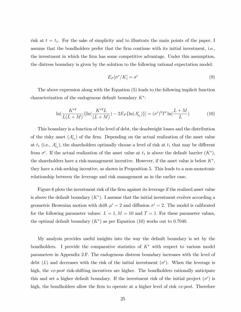
Figure 6 plots the investment risk of the firm against its leverage if the realized asset value

is above the default boundary (K∗). I assume that the initial investment evolves according a

geometric Brownian motion with drift µi = 2 and diffusion σi = 2. The model is calibrated

for the following parameter values: L = 1,M = 10 and T = 1. For these parameter values,

the optimal default boundary (K∗) as per Equation (10) works out to 0.7040.

My analysis provides useful insights into the way the default boundary is set by the

bondholders. I provide the comparative statistics of K∗ with respect to various model

parameters in Appendix 2.F. The endogenous distress boundary increases with the level of

debt (L) and decreases with the risk of the initial investment (σi). When the leverage is

high, the ex-post risk-shifting incentives are higher. The bondholders rationally anticipate

this and set a higher default boundary. If the investment risk of the initial project (σi) is

high, the bondholders allow the firm to operate at a higher level of risk ex-post. Therefore

25

Figure 6: This figure plots the optimal investment risk of the firm for the endogenous distress boundary. The model hasbeen calibrated for the following parameter values: L = 1,M = 10, T 0 = 1. The endogenous distress boundary is estimated atK = 0.7040.

they set a lower distress boundary. The relationship between the distress boundary and

deadweight losses is U-shaped, as I show numerically in Figure 7. As discussed in Section

3.4, the optimal investment risk at t = t1 is U-shaped in the deadweight losses. To offset this

effect, the bondholders set a distress boundary that is also U-shaped in K∗. The net effect

of the two results in the desired level of investment risk (σi) ex-post.

5 Empirical Evidence

5.1 Sample Selection and Data

I test the key predictions of my model, along with the predictions of the existing models

of corporate risk-management, using a comprehensive dataset. My sample covers the risk-

management activities of over 3,000 non-financial firms during the fiscal years 1996 and

1997.26 The data used in this study have been collected from the 10-K filings. First, I

26In 1994, the Financial Accounting Standard Board (FASB) issued SFAS 119. SFAS 119 requiredfirms to disclose the amount and type of derivative instruments held for trading and non-tradingpurposes separately. SFAS 119 covers firms with assets greater than $150 million. The smaller firmsare required to report their derivative usage as per SFAS 105 and 107. Since the implementation

26

Figure 7: This figure plots the level of endogenous distress boundary as a function of the deadweight losses of the firm. Themodel has been estimated for the following parameter values: The drift and diffusion of the initial investment (Ai) has beenset at 2 each, At1 = 1, L = 1 and T 0 = 1.

obtain all 10-K filings from the SEC for the calender year 1997.27 I remove utilities and

financial firms (SIC codes between 4910-4940 and 6000-6999 respectively) from the original

sample, since the risk-management activities of these firms are not directly comparable to

those of other firms. I also remove firms with market capitalization of less than $25 million

as of the fiscal year end. This facilitates the collection of data by hand. For the remaining

firms, I search the entire 10-K filings for the following text strings: "risk management,"

"hedg," "derivative" and "swap." If a reference is made to any of these key words, I read the

surrounding text to obtain data on interest rate and foreign currency derivative holdings. I

focus on interest rate and foreign currency derivatives since the reporting requirement for

commodity derivatives doesn’t allow for an easy quantification in terms of dollar value. This

is in line with earlier studies in the risk-management literature (see Geczy et al. (1997) and

Graham and Rogers (2002)).

I obtain data on the notional amount of derivatives used for non-trading (or risk-management)

purposes across various hedging instruments such as swaps, forwards and options.28 If there

of SFAS 119 in December 1994, the disclosure quality of derivative usage by the non-financial firmsincreased significantly. I choose fiscal years 1996 and 1997 for my study due to this reason.27For some firms (most of the firms with a fiscal year ending in October, November or December)

this corresponds to fiscal year 1996, while for others this corresponds to the fiscal year 1997.28The break-up of the notional amount across various instrument types was not easy to obtain for

27

are no references to the key words, the firm is classified as a non-hedger. I intersect this

database with the COMPUSTAT and CRSP databases. I need data on net sales, leverage

and market capitalization to be available for a firm to be included in the sample. The final

sample consists of 3,239 firms out of which 751 are classified as the hedgers. I use the no-

tional amount of interest rate and foreign currency derivatives scaled by the book value of

total assets as a measure of the risk-management activities of the firm. I call this variable

‘DERIVATIVES’ in the rest of the paper. This measure of hedging is consistent with the

earlier empirical studies that find evidence in support of risk-reducing (i.e, hedging) effect

of derivatives on various measures of a firm’s risk. For example, Guay (1999) finds that the

new users of derivatives experience a decline in their earnings and stock-price volatility after

the initiation of derivatives contract. Similarly Allayannis and Ofek (2001) show that using

derivatives reduces currency exposure.

The sample used in this paper is one of the most comprehensive in the literature. The

earlier studies have either used small samples or focused only on the binary decision of

hedging (i.e. the decision to hedge or not). For example, Graham and Rogers (2002) use

a sample of 442 firms out of which 158 are classified as hedgers; Geczy et al. (1997) use a

sample of 372 large firms out of which 154 firms are classified as hedgers. These studies over-

represent the big firms. My study is on the other hand more representative of the universe

of firms. My sample size is comparable to that of Mian (1996), who uses a sample of about

3,000 firms (771 firms classified as hedgers) and obtains data on hedging activities of these

firms from their 1992 annual reports. However, his study focuses only on the binary hedging

decisions. In contrast, I obtain data on the extent of hedging as well. As discussed later, my

findings are different from those of Mian (1996).

5.2 Descriptive Statistics

Table 1 provides the descriptive statistics of the hedging activities of 751 firms that are classi-

fied as hedgers. Panel A provides the summary statistics for the aggregate notional amount of

derivatives used for risk-management purposes. The mean (median) of the notional amount

some sample firms. For these firms, I collect data on the aggregate notional amount of derivativesonly. Since most of the analysis is conducted with the aggregate amount of derivatives, this doesn’tcreate any bias in the study.

28

of derivatives held for the risk-management purposes amounts to $ 416.12 million ($ 60 mil-

lion). The average level of derivatives-holdings for my sample firms is smaller than that of

earlier studies such as Graham and Rogers (2002) and Guay and Kothari (2002). This is not

surprising, since these studies have focused mostly on large firms as against my sample that

contains many medium and small firms as well. The notional value of derivatives scaled by

the book value of the firm’s total assets amounts to 12.66% (7.66%) for the average (median)

firm in the sample. These numbers are comparable to those of earlier studies.

Table 1 also provides the break-up of interest rate and foreign currency derivatives across

instrument types (Panels B and C). Swaps are the most widely used instrument for interest

rate derivatives, whereas forwards and futures contracts are the most widely used instruments

for managing foreign currency risks. About 85% of the interest rate hedgers use swaps,

whereas about 22% of them use options. Among the foreign currency hedgers, about 70%

of firms use forwards and futures contracts.

5.3 Selection of Explanatory Variables

The theory predicts a positive relationship between leverage and hedging for firms with

moderate levels of debt. The leverage ratio (LEVERAGE) of a firm is defined as the ratio of

total debt (long-term debt plus debt included in the current liabilities) to the book value of

total assets.29 My theory also predicts that firms with extreme leverage are unlikely to hedge.

To investigate the effect of extreme leverage on hedging, I include the square of the leverage

ratio (LEVERAGE-Squared) as an additional explanatory variable in the model. Since the

dependent variable (notional value of derivatives scaled by total assets) is censored at zero,

I use a Tobit regression to empirically analyze the effect of various explanatory variables on

the hedging activities of the firms. The theory predicts a positive sign on LEVERAGE and

a negative sign on LEVERAGE-Squared in the Tobit estimation.

My model predicts a positive relationship between leverage and hedging for firms with

high deadweight losses. However, this relationship reverses for very high levels of leverage.

I include two variables in the model to capture this effect - (a) an interaction term of the

29The results are similar for an alternative definition of leverage ratio that is based on the marketvalue of equity (i.e., the ratio of book value of total debt to the sum of book value of debt andmarket value of equity).

29

leverage ratio (LEVERAGE) and the inverse of the book-to-market ratio (1/BM) of the

firm and (b) an interaction term of the squared leverage ratio (LEVERAGE-Squared) and

the inverse of the book-to-market (1/BM) ratio. In line with the earlier empirical work,

I assume that low book-to-market firms experience higher deadweight losses of distress. I

expect to find a positive coefficient on LEVERAGE x 1/BM and a negative coefficient on

LEVERAGE-Squared x 1/BM.

5.3.1 Control Variables

The existing literature proposes frictions such as convexity of taxes (Smith and Stulz (1985)),

underinvestment costs (Froot et al. (1993)), managerial risk aversion (Smith and Stulz

(1985)) and information asymmetry between the managers and the outsiders of the firm

(DeMarzo and Duffie (1991,1995) and Breeden and Viswanathan (1998)) as alternative risk-

management motivations. In this section, I describe the construction of control variables

used in the study.

Economies of Scale: The earlier empirical studies find unanimous support for a strong

relationship between firm size and hedging activities. I include log of net sales of the firm as

a measure of its ‘SIZE.’ This variable capturers the effect of economies of scale in derivatives

usage.

Exposure to Risk: A firm’s hedging decision may depend on its exposure to interest rate

and foreign currency risk. All else equal, a firm with higher exposure to risk has a higher

incentive to engage in risk-management activities. If there are fixed costs associated with

the hedging activities, such a firm will face a lower per-unit cost of hedging. I include the

foreign currency sales as a percentage of total sales of the firm as a proxy for its exchange

rate risk exposure (‘FSALE’). To measure the firm’s exposure to the interest rate risk, I use

the ratio of floating rate debt to its total assets as an explanatory variable in the model

(‘FLOAT’). I expect a positive coefficient on both of these variables.

Tax-Based Incentives: If a firm faces a progressive tax structure, then its post-tax value

becomes a concave function of its pre-tax value. The firm can lower its expected tax li-

ability by engaging in hedging activities (Smith and Stulz (1985)). I use the methodol-

30

ogy suggested by Graham and Smith (1999) to measure the ‘TAX-CONVEXITY’ incentive

of hedging. A brief description of their methodology is provided in Appendix 2.G. The

‘TAX-CONVEXITY’ variable measures the expected tax benefits (in dollar value) by a 5%

reduction in income volatility of the firm. I scale this measure by the net sales of the firm.

The earlier empirical papers have used Net Operating Losses (NOL) carryforwards as a

proxy for the tax-based incentives of hedging. Graham and Rogers (2002) highlight some of

the limitations of using this variable as a proxy for tax-convexity. The firms with high levels

of NOL carryforwards have experienced losses in recent years. In the context of my model,

these firms can be identified with firms facing high levels of financial distress. Controlling for

the ‘TAX-CONVEXITY’ variable, I expect to find a negative association between hedging

and NOL carryforwards, as predicted by my model.

Underinvestment Costs: Froot et al. (1993) argue that hedging can benefit a firm by

reducing the underinvestment problem. In their model, external funds are costlier than

internally generated funds. The hedging activities reduce the firm’s dependence on the ex-

ternal sources of funds. Therefore, risk-management can increase firm value by mitigating

the underinvestment problem. Their model predicts a positive relationship between proxies

for underinvestment costs and the extent of hedging by the firm. I use two proxies to con-

trol for this effect - the book-to-market (BM) ratio of the firm and the ratio of research &

development (R&D) expenses to total sales. Froot et al. (1993) predict a negative relation-

ship between BM ratio and hedging and a positive relationship between R&D expenses and

hedging.30 If firms with low book-to-market ratio and high research & development (R&D)

expenses are more likely to lose their upside potential in the event of financial distress, my

model makes similar predictions with respect to these two variables.

The underinvestment problem of a firm can be reduced by keeping higher liquid assets.

Firms with greater short-term liquidity should have less dependence on the external sources

of funds. Therefore the relationship between measures of short-term liquidity and hedging

should be negative. I include the quick ratio of the firm (QUICK) as a measure of the firm’s

30In one of the unreported analyses, I also use the analyst growth forecast obtained from I\B\E\Sas a proxy for the growth option of the firm. Since my results remain qualitatively similar, I don’treport the results of this model.

31

liquid assets. The QUICK ratio is constructed as a ratio of cash and short-term investment

to the current liabilities of the firm. It measures the amount of funds that a firm can quickly

generate to meet its cash requirements. As in Geczy et al. (1997), I also use a measure of

dividend payout ratio to proxy for short-term liquidity. I use the dividend paid scaled by

the earnings before interest, depreciation, taxes and amortization (EBIDTA) of the firm to

construct the ‘DIVIDEND-PO’ variable.

Information Asymmetry: I include institutional shareholdings as an explanatory vari-

able in the model to control for the risk-management incentives due to information asym-

metry between the insiders and the outsiders of the firm. The ‘INSTITUTION’ variable

measures the fraction of the common shares of the firm that is held by the institutional

investors. The data is obtained from the 13-F filings. Assuming that higher institutional

shareholding leads to lower information asymmetry between the insiders and the outsiders of

the firm, the coefficient on this variable should be negative (DeMarzo and Duffie (1991,1995)).

Managerial Motivations: Smith and Stulz (1985) argue that hedging can increase the

expected utility of risk-averse managers if they hold large numbers of shares in the firm. On

the other hand, if managers hold large quantities of stock options, they may be induced to

pursue a risk-seeking behavior since option value increases with firm risk. In line with Geczy

et al. (1997), I use the log of the market value of equity held by the managers as a proxy

for their equity stake in the firm. I use the log of the Black-Scholes value of their options

grant as a proxy for their option-holding. These data are obtained from the COMPUSTAT

Executive Compensation database and are available for only a small subset of the sample

firms. I conduct a robustness test on the smaller subset of these firms. My results remain

similar for this model, but the test-statistics are lower due to smaller sample size. I do

not explicitly control for this variable in the main analysis of the paper since it results

in a loss of almost three-fourths of the sample firms. I do, however, control for industry

dummies in my analysis. If managerial compensation is largely determined by industry and

firm characteristics (such as the size and book-to-market ratio), my analysis has an implicit

control for the managerial motivations of hedging.

32

5.4 Univariate Tests

Table 2 presents some univariate results across the samples of hedgers and non-hedgers. I

find that the hedgers have significantly different characteristics from the non-hedgers. As

reported in the earlier studies, the hedgers are significantly larger firms both in terms of their

sales and market capitalization. The median market capitalizations of the hedger and the

non-hedger samples are $ 770 million and $ 140 million, respectively. The mean (median)

leverage ratio for the hedgers is 0.28 (0.25) which is significantly higher than the mean

(median) leverage ratio of 0.19 (0.12) for the non-hedgers. I don’t find any difference in the

book-to-market ratios of the two groups. The hedgers keep lower liquid assets as compared

with the non-hedgers as shown by the quick ratios of the two groups.

As expected, the hedgers have higher floating rate debts and foreign currency sales as

compared with the non-hedgers. The hedgers have lower NOL carryforwards. The median

institutional shareholding for the hedger sample is about 55% as against 35% for the non-

hedgers. The overall evidence from the univariate analysis suggests that the median hedger-

firm is a large firm with a high level of debt and high exposure to the interest rate and

foreign currency risk.

5.5 Tobit Regression

I use a Tobit regression analysis to analyze the effect of various explanatory variables on the

hedging activities of the firms. Since the dependent variable is censored at zero, the Tobit

regression provides a suitable empirical methodology (see Maddala(1983)). The model can

be represented by the following equation:

DERIV ATIV ES = α0 + α1 ∗ SIZE + α2 ∗ LEV ERAGE + α3 ∗ LEV ERAGE2 + α4 ∗QUICK + α5 ∗BM+α6 ∗ LEV ERAGE x 1/BM + α7 ∗ LEV ERAGE2 x 1/BM + α8 ∗ TAX −CONV EXITY

+α9 ∗DIV IDEND − PO + α10 ∗R&D + α11 ∗ FSALE + α12 ∗ FLOAT + α13 ∗NOL

+α14 ∗ INSTITUTION + (11)

In the above equation ‘DERIV ATIV ES’ is a censored dependent variable. It takes a

value of zero for the non-hedgers and the notional amount of derivatives scaled by total assets

for the hedgers. The independent variables are as described earlier. It has been argued in

33

the literature that the leverage decision should be endogenous in the models analyzing the

risk-management activities of the firm. I use a simultaneous equation method to address

this issue empirically.31 First, I need a structural model for the capital structure choice

of the firm. I follow Titman and Wessels (1988) and earlier empirical studies in the risk

management literature (Geczy et al. (1997) and Graham and Rogers (2002)) to obtain the

following structural model of the leverage ratio:

Leverage = β0 + β1 ∗DERIV ATIV ES∗ + β2 ∗ SIZE + β3 ∗R&D + β4 ∗ SGA+ β5 ∗ In tan gibles+ β6 ∗ ITC+β7 ∗MTR+ β8 ∗ PPE + β9 ∗Neg_BM +Σi=61i=1 γi ∗ INDi (12)

DERIV ATIV ES∗ is the predicted value of derivatives used for hedging, obtained from

the first stage estimation. The ‘SIZE0 and ‘R&D0 variables measure firm size and the

research and development expenses respectively. These variables are constructed as explained

before. ‘SGA0 measures the selling, general and administrative expenses as a percentage of

the sales; ‘In tan gibles’ is the book value of intangible assets as a percentage of the book

value of total assets; ‘ITC’ measures the investment tax credit as a percentage of total assets;

‘MTR’ refers to the before-financing simulated marginal tax rates (see Graham, Lemmon

and Schallheim (1998));32 ‘PPE’ stands for net book value of property, plant and equipment

scaled by the total assets; ‘Neg_BM ’ is a dummy variable indicating the negative book-

to-market firms. Finally, I include 61 industry dummy variables corresponding to the firm’s

two-digit SIC codes.

I estimate Models (11) and (12) simultaneously. First, the model for the leverage choice

(12) is estimated using an OLS technique. In the second stage, the risk-management equation

(11) is estimated using the predicted value of leverage ratio as the explanatory variable in

the Tobit estimation.31I also conduct the analysis without the endogeneity correction and the results are similar. To

save space, I present my findings for the endogeneity-corrected model only. For the model withoutthe endogeneity correction, I find a coefficient (p-value) of 0.27 (0.01) on the ‘Leverage Ratio’ and acoefficient of -0.14 (0.01) on the ‘Leverage Ratio - Squared’. For the smaller sub-sample (about 800observations), I also include managerial shareholding and optionholding variables in the regression.For this sub-sample, the coefficient estimates (p-value) on the ‘Leverage Ratio’ and the ‘LeverageRatio - Squared’ are 0.27 (0.03) and -0.25 (0.22), respectively.32I thank John Graham for providing me with his simulated marginal tax rates data for this

study.

34

5.5.1 Empirical Results

I present the results of the Tobit regression in Table 3. I present estimation results for

four models with different combinations of the explanatory variables. These models produce

similar results. I focus on Model 1 of Table 3 for most of the discussions in the paper. I find

a positive and significant coefficient on the leverage ratio (coefficient estimate of 0.3986 with

a p-value of 0.01). This is consistent with the prediction of my model as well as of the earlier

theoretical models based on financial distress costs (Smith and Stulz (1985)). Consistent

with the predictions of my model, the coefficient on leverage-squared is negative (-0.2710)

and significant (p-value=0.01).

This is the first large-sample evidence in support of the risk-management theories based

on the costs of financial distress or bankruptcy.33 Earlier studies provide mixed evidence.

While Booth, Smith and Stolz (1984), Haushalter (2000) and Graham and Smith (2002)

find some evidence in support of these theories, other studies such as Nance, Smith and

Smithson (1993), Mian (1996) and Tufano (1996) do not find such evidence. The studies

by Nance et al. (1993) and Graham and Smith (2002) are based on small samples. Tufano

(1996) and Haushalter (2000) use observations from the same industry (gold mining and oil

and gas respectively) and their results are also based on small samples. Mian’s sample size

is comparable to that of this study, but his study focuses only on the binary (i.e., yes-no)

decision of hedging and finds no support for the theory.

If there is a non-monotonic relationship between hedging and the financial distress costs,

small-sample studies may fail to produce a positive relationship between hedging and leverage

in the presence of a few firms with very high leverage. On the other hand, the large-sample

studies that analyze only the binary hedging decisions of the firm fail to take into account

the extent of hedging by the sample firms. Since the theoretical models generate predictions

about the extent of hedging by the firms, a study based only on the yes-no hedging decision

may fail to capture the essence of these theories. Based on a large sample of firms and by

analyzing the extent of hedging, my study provides strong evidence in support of a positive

33Purnanandam (2003) provides large-sample evidence in support of these theories by analyzingthe risk-management activities of commercial banks. In this paper, on the other hand, I provideevidence from non-financial firms.

35

relationship between leverage and hedging. Further, consistent with my theory, I find a

non-monotonic relationship between the two.

To gain further insight into the non-monotonicity of leverage and hedging activities, I

conduct a semi-parametric test. I break the sample of firms into deciles based on their

leverage ratios and run piecewise regressions (spline regression) across three groups - (i) low

leverage group (firms in deciles 1-5); (ii) moderate-to-high leverage group (deciles 6-9) and

(iii) extremely leveraged group (decile 10). For the first group (low leverage) the marginal

effect of leverage on hedging is positive (0.0325). The relation remains positive for the second

group (moderate-to-high leverage) with marginal effect of 0.1085. However, the marginal

effect of leverage on hedging becomes negative (-0.044) for the firms in top decile. The semi-

parametric test confirms the non-monotonic relation obtained in parametric regressions and

shows that the relation between leverage and hedging becomes negative for firms in top 10%

of distress likelihood.

I find a strong relationship between firm size and hedging. This finding is consistent with

the view that there are economies of scale in derivative usage (see Dolde (1993)). There is

a strong relationship between hedging and the extent of interest rate and foreign currency

risks faced by firms. Firms that derive higher fractions of their sales in the international

market hedge more than others. Similarly, a higher level of floating rate debt leads to a

higher level of hedging. Both these findings lend further support to the ‘economies of scale’

hypothesis of hedging.

The coefficients on the quick ratio and the book-to-market ratio are positive and insignif-

icant. This finding is not consistent with the underinvestment theories of hedging. However,

in line with these theories as well as my theory, the coefficient on the interaction of lever-

age and market-to-book ratio is positive and significant (p-value of 0.10). As in the case

of extreme leverage, I find a negative and significant coefficient on the interaction of the

leverage-squared variable and the market-to-book ratio. I also provide the estimation result

without the interaction of leverage-squared and market-to-book ratio in Model 2 of Table 3.

My main findings remain similar.

I don’t find any evidence in support of tax-based motivations for hedging. In contrast

to the theory’s prediction, firms with higher tax convexity hedge less than the others. This

36

finding is consistent with Graham and Rogers (2002). There is no evidence in support of

a positive relationship between R&D expenses and hedging. I find a positive relationship

between institutional shareholding and hedging. Assuming an inverse relationship between

institutional shareholding and the extent of information asymmetry between the insiders

and the outsiders of the firm, this result provides evidence against information-asymmetry-

based models of hedging. I find a negative relationship between hedging and NOL carry-

forwards. This finding is consistent with the prediction of my model that firms that have

experienced losses in the recent past hedge less. It is also consistent with the risk-shifting

argument of the model; i.e., firms with a very high likelihood of encountering distress have

no risk management incentives. Overall, my results suggest that the economies of scale and

financial distress costs are the two most important determinants of the hedging activities of

non-financial firms. There is a non-monotonic relationship between hedging and leverage.

Firms with very high leverage and firms that have experienced losses in the recent past are

less likely to hedge.

5.5.2 Risk Management across Large and Small Firms

The results provided in the previous section are based on the entire sample. I find that

the firm-size is an important determinant of firms’ hedging activities. Though I control

for the size of a firm in the Tobit regression, a pooled regression (across all firms) analysis

may hide the hedging behavior of large and small firms if they have significantly different

characteristics and hedging motivations. To shed further light on such corporate hedging

behavior, I divide the sample into two groups based on whether the firm size (as measured

by the net sales) is above or below the sample median. There are about 1,500 firms in both

groups with 583 hedgers in the sample of large firms and 111 hedgers in the sample of small

firms. The second-stage estimation results of the Tobit model are provided in Table 4.

The analysis provides several new insights into the hedging behavior of large and small

firms. While firm size and leverage ratio explain the risk-management decisions of both

groups, other theories of risk-management do a reasonably good job of explaining the hedging

behavior of the large firms. As shown in Table 4, the coefficients on size, leverage and

leverage-squared variables are comparable across the two groups. Similarly, both groups

have positive and significant coefficients on the proxies for exposure to the interest rate and

37

foreign currency risks. These results are in line with the results for the overall sample.

The large firms use liquid assets as a substitute for the hedging activities as evident by

a negative and significant sign on the quick ratio. For this sample, I find a positive and

significant coefficient on the R&D variable. Both these findings are consistent with the

underinvestment cost model of Froot et al. (1993). I don’t find similar evidence for the

small firms. Unlike large firms, these firms seem to complement their hedging strategies

with liquid assets. There is some evidence in support of the tax-based theories of hedging

for the sample of large firms. While the small-firm sample has a negative coefficient on the

tax-convexity measure, the large-firm sample shows a positive coefficient (with p-value of

0.06) on this variable. The results with respect to other variables are qualitatively similar

across the two samples.

5.5.3 Ex-ante Exposure to Risk

Are my results affected by the inclusion of firms without any exposure to interest rate or

foreign currency risk in the sample? For a firm with no exposure to interest rate or foreign

currency risk, the absence of risk-management instruments is simply a consequence of no

exposure and not a choice made by the firm. Since I am interested in studying the firm’s

risk-management decision making, my analysis may be biased by the inclusion of such firms

in the sample. To address this issue, I conduct a robustness test by including only those

firms in the sample that have a well-defined ex-ante exposure to the risks.

I follow Geczy et al. (1997) to investigate the ex-ante exposure to foreign currency risk

and Graham and Rogers (2002) for interest rate risk. A firm is classified as being exposed to

foreign currency risk if any of the following criteria are met: (a) it reports foreign currency

sales in the COMPUSTAT geographic segment file in any of the three fiscal years including

the current fiscal year and one year before and after the current year; (b) it reports some

amount of foreign income taxes, foreign currency adjustments, deferred foreign currency taxes

or pretax foreign income in its annual statements; (c) it reports foreign currency adjustments

in its annual report; or (d) the firm is a hedger of foreign currency risk.34

34Geczy et al. (1997) also consider firms with high concentration of foreign importers in theindustry as exposed to foreign currency risk. I don’t consider this screening criterion since they

38

In order to identify firms with ex-ante exposure to interest rate risk, I regress the changes

in operating income on the changes in the six-month Treasury yield. I use the past seven

years of quarterly data for each firm’s regression. A firm is classified as being exposed to

interest rate risk if any of the following conditions hold: (a) the regression coefficient on the

Treasury yield variable is significant at the 10% level; (b) the firm has long-term floating

debt; (c) the firm has short-term borrowings; or (d) the firm is a hedger of interest rate risk.

The resulting sample, with exposure to either interest rate or foreign currency risk com-

prises about 2,600 firms. The estimation result for this sample is provided in Table 5. The

results remain similar to those of the base case. There is a positive and significant rela-

tionship between hedging and leverage and a negative and significant relationship between

hedging and leverage-squared. Other results are also similar.

5.5.4 Industry Adjusted Leverage Ratios

As a further robustness, I conduct the analysis with the industry-adjusted leverage ratios

of the firms. The theory predicts a positive relationship between leverage and hedging for

moderate levels of leverage. The level of leverage may vary considerably across industries.

An industry adjustment provides a more robust way to classify firms into those having a

moderate and those having a high level of leverage. I compute the industry median leverage

ratio based on 2-digit SIC codes. The industry-adjusted leverage ratio of a firm is defined as

the difference between the firm leverage and the industry median ratio. I re-estimate all my

results with these ratios. The main findings of the paper remain robust, as seen in Table 6.

6 Conclusion

This paper develops a theory of corporate risk management in the presence of deadweight

losses caused by financial distress. By distinguishing ‘financial distress’ from ‘insolvency’,

I provide a justification for the ex-post risk management behavior of the firm. Due to the

deadweight losses from financial distress, the shareholders engage in ex-post risk-management

show that there are very few firms that are identified to have foreign currency exposure basedsolely on this criterion. In their sample of about 370 firms, only three firms were identified to haveexposure based on this criteria.

39

activities even without a pre-commitment to do so. The theory is based on a trade-off be-

tween the shareholders’ risk-shifting incentives due to equity’s limited liability and their

risk-avoidance incentives due to the deadweight losses of financial distress. I obtain an op-

timal level of investment risk, from the shareholders’ perspective, based on this trade-off.

The model generates several testable predictions. It predicts a non-monotonic relation-

ship between leverage and hedging. The relationship between deadweight losses and risk-

management activities is predicted to be U-shaped. In my model, firms with higher financial

distress barriers and longer time horizons have greater hedging incentives.

I test the predictions of my model as well as the predictions of the existing theoretical

models with one of the most comprehensive samples used in the literature. Using a sample

of over 3,000 non-financial firms, I find strong evidence in support of a positive relationship

between leverage and hedging. Consistent with the theory, this relationship becomes negative

for firms with high very leverage. Similarly, the relationship between leverage and hedging

is non-monotonic for high market-to-book value firms. In line with the theory, I find that

firms that experienced losses in the recent past hedge less.

My empirical study provides the first-large sample evidence on the extent of hedging by

non-financial firms. I find that large and small firms hedge for different reasons. While both

groups hedge in response to financial distress costs and show non-monotonicity in the rela-

tionship between leverage and hedging, extant risk-management theories do a reasonable job

of explaining the risk-management behavior of large firms. The large-firm sample provides

evidence in support of the underinvestment cost theories of hedging. It also provides some

evidence in support of the tax-based theories. The hedging behavior of small firms, on the

other hand, is explained primarily by economies of scale and financial distress costs.

This paper can be extended in several directions. Since I focus on the risk-management

activities of the firm in this paper, I take the capital structure decision as exogenous to

the model. The capital structure decision can be endogenized to generate insights into the

interaction of a firm’s risk-management activities with its capital structure decisions. In

such a model, one can also analyze the optimal determination of debt-covenants, from the

bondholders’ perspective, in the presence of agency cost of risk-shifting.

The empirical results show that large and small firms hedge for different reasons. What

40

may explain this, apart from the economies of scale? The issue can be explored further by

analyzing the hedging behavior of two groups in greater detail. Finally, using the compre-

hensive dataset of hedging, I can shed light on the untested implications of many theoretical

models in the risk-management literature. For example, one can analyze questions such as

‘how (i.e., what type of hedging instruments) do firms hedge?’ and ‘how does the managerial

compensation affect a firm’s risk management policies?’ These questions have been left for

future research work.

41

References[1] Allayannis, G. and E. Ofek, 2001, "Exchange Rate Exposure, Hedging, and the Use of Foreign

Currency Derivatives", Journal of International Money and Finance 20, 273-296.

[2] Andrade, G. and S. Kaplan, 1998, "How Costly is Financial (Not Economic) Distress? Evi-dence from Highly Leveraged Transactions that became Distressed", Journal of Finance 53,1443-1493.

[3] Anderson, R. W. and S. M. Sundaresan, 1996, ”The Design and Valuation of Debt Contracts,”Review of Financial Studies 9,37-68.

[4] Arping, S., 2000, "Debt and Product Market Fragility", Working Paper, HEC, Lausanne.

[5] Booth, J. R., R. L. Smith and R. W. Stolz, 1984, "The Use of Interest Rate Futures byFinancial Institutions", Journal of Bank Research 15, 15-20.

[6] Breeden, D. and S. Viswanathan, 1996, "Why do Firms Hedge? An Asymmetric InformationModel", Working Paper, Duke University.

[7] Brockman, P. and H. J. Turtle, 2003, "A Barrier Option Framework for Corporate SecurityValuation", Journal of Financial Economics 67, 511-529.

[8] Duffie, D., 1996, Dynamic Asset Pricing Theory, Princeton University Press.

[9] DeMarzo, P. M. and D. Duffie, 1991, "Corporate Financial Hedging with Proprietary Infor-mation", Journal of Economic Theory 53, 261-286.

[10] DeMarzo, P. M. and D. Duffie, 1995, ”Corporate Incentives for Hedging and Hedge Account-ing,” Review of Financial Studies 8, 743-771.

[11] Diamond, D. W., 1991, "Debt Maturity Structure and Liquidity Risk", Quarterly Journal ofEconomics 106, 709-737.

[12] Dichev, I. D. and D. J. Skinner, 2001, "Large-Sample Evidence on the Bond Covenants Hy-pothesis", Working Paper, University of Michigan.

[13] Dolde, W., 1993, "The Trajectory of Corporate Financial Risk Management", Journal ofApplied Corporate Finance 6, 33-41.

[14] Fehle, F. and S. Tsyplakov, 2003, "Dynamic Risk Management : Theory and Evidence",Working Paper, University of South Carolina.

[15] Froot, K. A., D. S. Scharfstein and J.C. Stein, 1993, "Risk Management: Coordinating Cor-porate Investments and Financing Policies", Journal of Finance 5, 1629-1658.

[16] Geczy, C., B. A. Minton and C. Schrand, 1997, "Why Firms Use Currency Derivatives?",Journal of Finance 52, 1323-1354.

[17] Graham, J. R., M. L. Lemmon and J. S. Schallheim, 1998, "Debt, Leases, Taxes and theEndogeneity of Corporate Tax Status", Journal of Finance 53, 131-162.

42

[18] Graham, J. R. and D. A. Rogers, 2002, "Do Firms Hedge in Response to Tax Incentives",Journal of Finance 57, 815-839.

[19] Graham, J. R. and C.R. Smith, 1999, "Tax Incentives to Hedge", Journal of Finance 54,2241-2262.

[20] Guay, W., 1999,"The Impact of Derivatives on Firm Risk: An Empirical Examination of NewDerivatives Users", Journal of Accounting and Economics 26, 319-162.

[21] Guay, W. and S.P.Kothari, 2002, "How Much Do Firms Hedge with Derivatives?", Journal ofFinancial Economics, Forthcoming.

[22] Harrison, J. M., 1985, "Brownian Motion and Stochastic Flow Systems", Wiley, New York.

[23] Haushalter, D. G., 2000,"Financing Policy, Basis Risk, and Corporate Hedging: Evidencefrom Oil and Gas Producers", Journal of Finance 55,107-152.

[24] Jarrow, R. and A. Purnanandam, 2003, "Capital Structure and the Present Value of a Firm’sInvestment Opportunities", Working Paper, Cornell University.

[25] Jensen, M.C. and W. H. Meckling, 1976, "Theory of the Firm: Managerial Behavior, AgencyCosts and Ownership Structure", Journal of Financial Economics 3,305-360.

[26] Kalay, A., 1982, "Stockholder-Bondholder Conflict and Dividend Constraints", Journal ofFinancial Economics 10, 211-233.

[27] Lamont, O., 1997, "Cash Flow and Investments : Evidence from Internal Capital Markets",Journal of Finance 52, 83-109.

[28] Leland, H. E., 1998, "Agency Costs, Risk Management, and Capital Structure", Journal ofFinance 53, 1213-1243.

[29] Maddala, G.S.,1983, "Limited Dependent and Qualitative Variables in Econometrics", Econo-metric Society Monographs, Cambridge University Press.

[30] Mella-Barral, P., 1999, ”The Dynamics of Default and Debt Reorganization,” Review of Fi-nancial Studies 12, 535-578.

[31] Mella-Barral, P., and W. R. M. Perraudin, 1997, ”Strategic Debt Service,” Journal of Finance52, 531-556.

[32] Mian, S. L., 1996, "Evidence on Corporate Hedging Policies", Journal of Financial and Quan-titative Analysis 31, 419-439.

[33] Moody’s Investors Service Report, 1998, ”Historical Default Rates of Corporate Bond Issuers,1920-1997.”

[34] Morellec, E. and C.W. Smith, 2003, "Investment Policy, Financial Policies, and the Controlof Agency Conflicts", Working Paper, University of Rochester.

[35] Mozumdar, A., 2001, "Corporate Hedging and Speculative Incentives: Implications for SwapMarket Default Risk", Journal of Financial and Quantitative Analysis 36, 221-250.

43

[36] Musiela, M. and M. Rutkowski, 1998, "Martingale Methods in Financial Modelling", SpringerVerlag Publications.

[37] Myers, S., 1977, "Determinants of Corporate Borrowing", Journal of Financial Economics 4,147-176.

[38] Myers, S. C. and N. Majluf, 1984, "Corporate Financing and Investment Decisions WhenFirms Have Information Investors Do Not Have", Journal of Financial Economics 13, 187-221.

[39] Nance, D. R., C. W. Smith and C. W. Smithson, 1993, "On the Determinants of CorporateHedging", Journal of Finance 48, 267-284.

[40] Opler, T. and S. Titman, 1994, "Financial Distress and Corporate Performance", Journal ofFinance 49, 1015-1040.

[41] Petersen, M. and S.R. Thiagarajan, 2000, "Risk Measurement and Hedging: with and withoutDerivatives", Financial Management 29, 5-30.

[42] Purnanandam, A., 2003, "Do Banks Hedge in Response to the Financial Distress Costs?",Working Paper, Cornell University.

[43] Robicheck, A. A., and S. C. Myers, 1966, ”Problems in the Theory of Optimal Capital Struc-ture,” Journal of Financial and Quantitative Analysis, 1, 1-35.

[44] Shapiro, A. and S. Titman, 1986, "An Integrated Approach to Corporate Risk Management",in Joel Stern and Donald Chew, eds: The Revolution in Corporate Finance (Basil Blackwell,LTD, England).

[45] Smith, C. and R. Stulz, 1985, "The Determinants of Firms’ Hedging Policies", Journal ofFinancial and Quantitative Analysis, 28, 391-405.

[46] Smith, C. W. and J. B. Warner, 1979, "On Financial Contracting: An Analysis of BondCovenants", Journal of Financial Economics 7, 117-161.

[47] Stulz, R., 1984, "Optimal Hedging Policies", Journal of Financial and Quantitative Analysis19,127-140.

[48] Stulz, R., 1996, "Rethinking Risk Management", Journal of Applied Corporate Finance 9,8-24.

[49] Titman, S., 1984, "The Effect of Capital Structure on a Firm’s Liquidation Decision", Journalof Financial Economics 13, 137-151.

[50] Titman, S. and R. Wessels, 1988, "The Determinants of Capital Structure Choices", Journalof Finance 43, 1-19.

[51] Tufano, P., 1996, "Who Manages Risk? An Empirical Examination of Risk ManagementPractices in the Gold Mining Industry", Journal of Finance 51,1097-1137.

[52] Whited, T., 1992, "Debt, Liquidity Constraints, and Corporate Investments : Evidence from

Panel Data", Journal of Finance 47, 1425-1460.

44

APPENDIX - 1

Anecdotal Evidences on Deadweight Losses of Financial Distress

1. Delta Airlines: In mid-2002, Delta Airlines breached a debt-to-equity ratio covenantrequired by one of its borrowing agreements. In order to have this covenant waived, the firm was

required to keep cash and cash equivalents of $ 1 billion at the end of every month from October

2002 until June, 2003. According to CBS Marketwatch, September 2002 ‘.....in order to have the

debt-to-equity part of the covenant waived, Delta has agreed to maintain a minimum of $1 billion

in cash and cash equivalents at the end of every month, starting in October. This will handicap

the company’s cash to spend, weakening a balance sheet Delta once touted as its strong point...’

Delta’s 10-K filing for year 2002 further states: "...In October 2002, we amended our unsecured

letter of credit Reimbursement Agreement with Commerzbank AG and a group of banks to (1)

eliminate the debt-to-equity ratio and secured debt covenants from that agreement and (2) adda covenant requiring us to maintain a minimum of $1 billion of unrestricted cash,cash equivalents and short-term investments as of the end of each month, beginningon October 31, 2002. The Reimbursement Agreement and the related letters of credit willterminate on June 8, 2003....".

2. Apple Computers: Apple Computers experienced a decline of 27% in the unit sales of

Mac Computers from 1997 to 1998. Both industry observers (see Business Week, January 29, 1996

and February 05, 1996, and Arping (2000)) and the firm attributed a part of this decline to its

poor financial performance. Apple Computer’s 10-K filings for 1998 states: "..Decisions by cus-

tomers to purchase the Company’s personal computers, as opposed to Windows-based systems, are

often based on the availability of third-party software for particular applications. The Company be-

lieves that the availability of third-party application software for the Company’s hardware products

depends in part on third-party developers’ perception and analysis of the relative benefits of devel-

oping, maintaining, and upgrading such software for the Company’s products versus software for

the larger Windows market. This analysis is based on factors such as the perceived strength of the

Company and its products, the anticipated potential revenue that may be generated, and the costs

of developing such software products. To the extent the Company’s financial losses in prioryears and declining demand for the Company’s products, as well as the Company’sdecision to wind down its Mac OS licensing program, have caused software develop-ers to question the Company’s prospects in the personal computer market, developerscould be less inclined to develop new application software or upgrade existing softwarefor the Company’s products and more inclined to devote their resources to developingand upgrading software for the larger Windows market."...

3. K-Mart: Prior to the bankruptcy filings of K-Mart, in late 2001 and early 2002, severalsuppliers stopped extending trade credit to the firm. As reported in the Wall Street Journal,

45

January 21, 2002: "...Fleming Cos., a key food supplier to Kmart Corp., joined the growing list of

suppliers to cut off shipments for the struggling retailer. Fleming said Monday that it suspended

the shipments because Kmart had missed a weekly payment but that it is working with the chain

as it navigates through its financial problems....".

4. International Harvester: When International Harvester, a heavy farm equipment pro-

ducer, experienced financial difficulties in the early 1980s, it lost business to its competitors mainly

due to customers’ fear about getting parts and services. The Wall Street Journal (October 11, 1982)

reports that "the closing of some dealership is causing a few customers to worry about getting parts

and services" (quoted in Titman (1984)).

5. Wyndham Inc: In 2001, Wyndham, a hotel and resort company, approached its lenders forwaiver of certain debt-covenants on its $ 3.3 billion bank debt. In order to get the covenants waived,

the firm had to agree to limit its dividends, lose flexibility in its operations and reduce its credit-

lines. As reported by the Wall Street Journal (October 15, 2001): "...Wyndham’s bank syndicate

consists of more than 50 lenders, led by J.P. Morgan Chase. Wyndham told its bankers it needed

two quarters of covenant relief to assess the long-term damage to the hotel industry, according to

one banker. After some debate within the bank group about how much additional protection to

demand in return, Wyndham’s lenders agreed to waive certain covenants for the third and fourth

quarters, and to aim for a long-term amendment by Feb. 28. In exchange, Wyndham agreed todefer cash dividend payments on its preferred stock, to limit capital spending beforeFeb. 28 to $85 million, to apply all cash proceeds from asset sales to loan repayments,and to reduce its revolving credit line to $400 million from $500 million....".

46

APPENDIX - 2

A Proof of Proposition 1:Proof. Shareholders payoff on the terminal date (T ) is given by the following:

ξT = (AT − L)1AT>L,mT>K + (f(AT )− L)1f(AT )>L,mT≤K= (AT − L)(1AT>L − 1AT>L,mT≤K) + (f(AT )− L)1f(AT )>L,mT≤K= (AT − L)1AT>L − (AT − L)1AT>L,mT≤K + (f(AT )− L)1f(AT )>L,mT≤K= (AT − L)1AT>L − (AT − L)[1f(AT )>L,mT≤K + 1f−1(L)>AT>L,mT≤K] + (f(AT )− L)1f(AT )>L,mT≤K= (AT − L)1AT>L − (AT − f(AT )1f(AT )>L,mT≤K + (L−AT )1f−1(L)>AT>L,mT≤K= (AT − L)− (AT − f(AT )1f(AT )>L,mT≤K + (L−AT )1AT≤L + 1f−1(L)>AT>L,mT≤K

The equity value at t = t1 (ξt1) is simply the expectation of this payoff under the martingalemeasure. Taking the expectation of the terminal payoff gives the desired result.QED.

B Equity-Valuation:As shown in expression (2) in the paper, the equity valuation is given by the following:

Et1 = EQ[(AT − L)1AT>L,mT>K + 1AT>L,AT≤L+M,mT≤K+M1AT>L+M,mT≤K]= EQ[(AT − L)1AT>L,mT>K + 1AT≤L+M,mT≤K − 1AT≤L,mT≤K+M1AT>L+M,mT≤K]= EQ[(AT − L)1AT>L − 1AT>L+M + 1AT>L+M,mT>K+M1AT>L+M,mT≤K] (B.1)

The first two components of the equity value, namely EQ[(AT−L)1AT>L] and EQ[(AT−L)1AT>L+M], can be computed using the standard Black-Scholes formula for the valuationof the European call options. Let Φ and φ stand for the normal cumulative density function(cdf) and probability density function (pdf) respectively. For notational simplicity I setAt1 = A0 and T 0 = T − t1. Then the first two terms result in the following expression:

EQ[(AT − L)1AT>L] = A0Φ(h1)− LΦ(h2) and EQ[(AT − L)1AT>L+M] = A0Φ(d1)− LΦ(d2)

Where,

h1 =ln(A0

L) + σ2

2T 0

σ√T 0

and h2 = h1 − σ√T 0

d1 =ln( A0

L+M) + σ2

2T 0

σ√T 0

and d2 = d1 − σ√T 0

The last two terms, i.e. EQ[(AT − L)1AT>L+M,mT>K] and EQ[M1AT>L+M,mT≤K], requirethe knowledge of the joint distribution of the running minima and the terminal value of thegeometric Brownian motion. Such distributions have been widely used for the pricing ofpath-dependent options. I use the following Lemma (see Harrison (1985) or Musiela andRutkowski (1998)) to obtain the expression for the valuation of these two path-dependentexpressions:

47

Lemma: Let K < L and K < A0, then the joint density of the terminal asset value (AT )and the running minima of the geometric Brownian motion (mT ), under the martingalemeasure, is provided by the following formula:

Q(AT> L,mT≥ K) = Φ(ln(A0

L)− σ2

2T 0

σ√T0 )− (A0

K)Φ(

ln( K2

A0L)− σ2

2T 0

σ√T 0

) (B.2)

Using (B.2), I compute the expectation of the last two terms of expression (B.1) asfollows:

EQ[(AT − L)1AT>L+M,mT>K)] = A0Φ(d1)− LΦ(d2)− KΦ(c1)− A0L

KΦ(c2)

EQ[M1AT>L+M,mT≤K)] =A0M

KΦ(c2)

where d1 and d2 are as given before and

c1 =ln( K2

A0(L+M)) + σ2

2T 0

σ√T 0

and c2 = c1 − σ√T 0

Collecting the above results and simplifying the expressions further, I get the followingexpression for the valuation of the firm’s equity at t = t1.

Et1 = A0Φ(h1)− LΦ(h2)− KΦ(c1)− A0(L+M)

KΦ(c2) (B.3)

C First-Order Condition:At the optima, the following first-order condition must be satisfied:

∂E0∂σ

= 0

Differentiating expression (B.5) gives the following:∂Et1∂σ

= A0φ(h1)∂h1∂σ

− Lφ(h2)∂h2

∂σ− Kφ(c1)

∂c1

∂σ− A0L

Kφ(c2)

∂c2

∂σ+ A0M

Kφ(c2)

∂c2

∂σ(C.1)

Note that:

φ(h2) =A0

Lφ(h1)

φ(c2) =K2

A0(L+M)φ(c1) (C.2)

(C.1) and (C.2) leads to the following:

∂Et1∂σ

= A0φ(h1)∂h1∂σ

−A0φ(h1)∂h1∂σ

−√T 0− Kφ(c1)

∂c1

∂σ− KL

(L+M)φ(c1)∂c1

∂σ−√T 0+ KM

(L+M)φ(c1)∂c1

∂σ−√T 0

Simplification leads to the following:

∂Et1∂σ

= A0φ(h1)√T 0 − φ(c1)K∂c1

∂σ− KL

(L+M)∂c1∂σ

−√T 0− KM

(L+M)∂c1∂σ

−√T 0

Thus I have the following first-order condition for the optimal investment risk of the firm:

A0φ(h1)√T − φ(c1)K

√T = 0 (C.3)

Thus,A0φ(h1)−Kφ(c1) = 0 (C.4)

48

D Second-Order Condition:

Differentiating expression (C.4) gives the second-order condition of optimality:∂2Et1∂σ2

= −h1A0φ(h1)√T 0

∂h1

∂σ+ c1φ(c1)K

√T 0

∂c1

∂σ(D.1)

Using the first-order condition and simplifying it further, the above expression, at theoptima, reduces to the following:

∂2Et1∂σ2

= −h1φ(c1)K√T 0

∂h1

∂σ+ c1φ(c1)K

√T 0

∂c1

∂σ

= φ(c1)K√T 0(−h1(

√T 0 − h1

σ) + c1(

√T 0 − c1

σ))

= φ(c1)K√T 0(h1 − c1)(h1 + c1 − σ

√T 0)

Using the following equalities:

(h1 − c1) =ln(

A20(L+M)

K2L)

σ√T 0

> 0 and (h1 + c1 − σ√T 0) =

ln( K2

L(L+M))

σ√T 0

< 0

It follows that∂2Et1∂σ2

< 0 (D.2)

Thus the second-order condition for the maximization problem is satisfied.

E Comparative Statistics:

Comparative statistics are obtained by a direct differentiation of the optimal solution for σgiven in expression 5.(a) Sensitivity with respect to default boundary (K):

∂(σ2)∗

∂K=

2

T 0K ln(L+ML

)ln( K2

L(L+M)) + ln(

K2L

A2t1(L+M)) < 0

The inequality follows from the facts that K < L,K < At1 and M > 0.

(b) Sensitivity with respect to initial asset value (At1) :

∂(σ2)∗

∂At1

= − 2

T 0At1 ln(L+ML

)ln( K2

L(L+M)) > 0

(c) Sensitivity with respect to time-to-maturity (T 0 = T − t1):

∂(σ2)∗

∂T 0= − (σ

2)∗

T 0< 0

(d) Sensitivity with respect to the deadweight loss parameter M :Direct differentiation of the optimal investment risk leads to the following:

∂(σ2)∗

∂M> 0 if M > L exp

2(

rln(

At1K

) ln( LK))−L

49

F Comparative Statistics for Endogenous Distress Bound-ary

As shown in Equation (10), the endogenous default boundary is given by the followingimplicit function:

G : (σi)2T 0 ln(L+M

L)− ln( K∗2

L(L+M))[ln(

K∗2L(L+M)

)− 2EP ln(Ait1)] = 0 (E.1)

Differentiating the above function with respect to K∗ I get the following:

∂G

∂K∗= − 2

K∗[ln(

K∗2L(L+M)

)− 2EP ln(Ait1)]− ln( K∗2

L(L+M))2

K∗

> 0 since EP ln(Ait1) > ln(K∗) in my model.

Using the implicit function theorem and the fact that ∂G/∂K∗ > 0 , the sensitivity of theendogenous distress boundary with respect to any model parameter (θ) can be given by thefollowing:

sign(∂K∗

∂θ) = −sign(∂G

∂θ)

1. Sensitivity with respect to the level of debt (L):

∂G

∂L= − (σ

i)2T 0ML(L+M)

+ [ln(K∗2L(L+M)

)− 2EP ln(Ait1)] (2L+M)

L(L+M)− M

L(L+M)ln(

K∗2

L(L+M))

After some simplification, this leads to ∂G/∂L < 0. Therefore:

∂K∗

∂L> 0

2. Sensitivity with respect to the initial asset risk (σ∗):Assuming that the initial investment (Ai) evolves as a geometric Brownian motion with

drift µi and diffusion σi, I get the following:

∂G

∂σi= 2σiT ln(

L+M

L)− 2σiT ln( K∗2

L(L+M)) > 0

Thus,∂K∗

∂σi< 0

G Tax-Convexity Measure

I use the methodology suggested by Graham and Smith (1999) to measure the tax-convexityincentive of hedging. Using the methods of simulation and considering the various featuresof tax codes, they compute the expected tax-benefits that would result from a 5% reductionin income volatility. Subsequently they perform a regression analysis that relates tax savingsto the following explanatory variables: (i) an indicator variable identifying taxable incomebetween -$500,000 and zero (TI(NEG)), (ii) an Indicator variable identifying taxable income

50

between zero and $500,000 (TI(POS)), (iii) income volatility measured as the absolute coef-ficient of variation (VOL), (iv) first-order serial correlation in income (RHO), (v) a dummyvariable indicating the existence of investment tax credit (ITC), (vi) a dummy variable in-dicating the existence of Net Operating Losses (NOL) carryforwards and finally (vii) NOLdummy interacted with the small-loss (NOL*TI(NEG)) and small-gain (NOL*TI(POS)) in-dicator variables. The regression estimates is given as follows:

Tax−Convexity = 4.88 + 7.15 ∗ TI(NEG) + 1.60 ∗ TI(POS) + 0.019 ∗ V OL− 5.50 ∗RHO − 1.28 ∗ ITC+NOL ∗ (3.29− 4.77 ∗ TI(NEG)− 1.93 ∗ TI(POS))

I obtain the predicted tax savings in dollars for each firm in the sample by using theabove equation. This is scaled by the sales of the firm to get the ’Tax-Convexity’ measure.

51

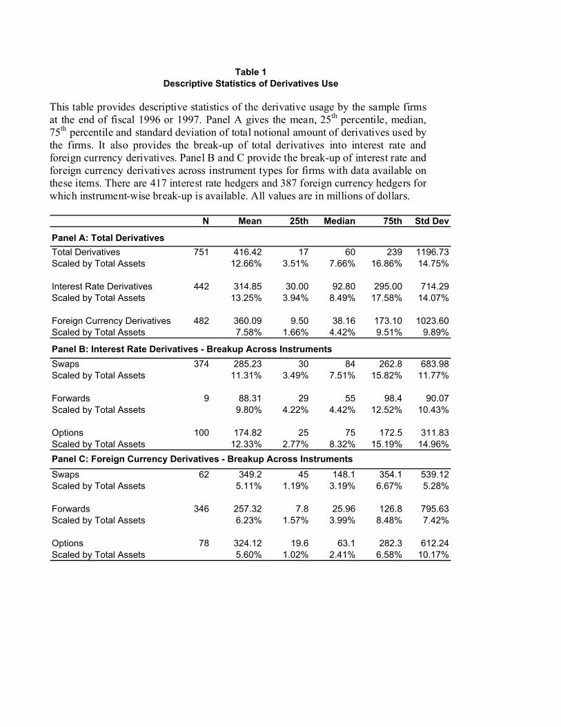
N Mean 25th Median 75th Std Dev

Panel A: Total DerivativesTotal Derivatives 751 416.42 17 60 239 1196.73Scaled by Total Assets 12.66% 3.51% 7.66% 16.86% 14.75%

Interest Rate Derivatives 442 314.85 30.00 92.80 295.00 714.29Scaled by Total Assets 13.25% 3.94% 8.49% 17.58% 14.07%

Foreign Currency Derivatives 482 360.09 9.50 38.16 173.10 1023.60Scaled by Total Assets 7.58% 1.66% 4.42% 9.51% 9.89%

Panel B: Interest Rate Derivatives - Breakup Across InstrumentsSwaps 374 285.23 30 84 262.8 683.98Scaled by Total Assets 11.31% 3.49% 7.51% 15.82% 11.77%

Forwards 9 88.31 29 55 98.4 90.07Scaled by Total Assets 9.80% 4.22% 4.42% 12.52% 10.43%

Options 100 174.82 25 75 172.5 311.83Scaled by Total Assets 12.33% 2.77% 8.32% 15.19% 14.96%Panel C: Foreign Currency Derivatives - Breakup Across InstrumentsSwaps 62 349.2 45 148.1 354.1 539.12Scaled by Total Assets 5.11% 1.19% 3.19% 6.67% 5.28%

Forwards 346 257.32 7.8 25.96 126.8 795.63Scaled by Total Assets 6.23% 1.57% 3.99% 8.48% 7.42%

Options 78 324.12 19.6 63.1 282.3 612.24Scaled by Total Assets 5.60% 1.02% 2.41% 6.58% 10.17%

Table 1Descriptive Statistics of Derivatives Use

This table provides descriptive statistics of the derivative usage by the sample firms at the end of fiscal 1996 or 1997. Panel A gives the mean, 25th percentile, median, 75th percentile and standard deviation of total notional amount of derivatives used by the firms. It also provides the break-up of total derivatives into interest rate and foreign currency derivatives. Panel B and C provide the break-up of interest rate and foreign currency derivatives across instrument types for firms with data available on these items. There are 417 interest rate hedgers and 387 foreign currency hedgers for which instrument-wise break-up is available. All values are in millions of dollars.

Variable N Mean Median Std Dev N Mean Median Std Dev. Mean Median

Sales (log $MM) 751 6.8262 6.7214 1.6203 2488 4.7723 4.7876 1.7129 0.01 0.01

Market Capitalization ($MM) 751 4605.83 777.71 14141.83 2488 523.92 140.75 1619.98 0.01 0.01

Leverage/TA 751 0.2755 0.2527 0.2047 2478 0.1875 0.1207 0.2176 0.01 0.01

EBIDTA/ Sales 748 0.1525 0.1377 0.1539 2484 -0.5431 0.1024 9.8982 0.05 0.01

Book-to-Market 750 0.4666 0.4148 0.7397 2488 0.4873 0.4075 0.4965 0.37 0.42

Quick Ratio 716 0.6028 0.1696 2.5620 2423 1.8481 0.5403 3.8945 0.01 0.01

Marginal Tax Rate(%) 681 0.3185 0.3500 0.0883 1945 0.2646 0.3437 0.1357 0.01 0.01

Tax Convexity/Sales 750 0.0130 0.0030 0.0362 2484 0.1204 0.0215 1.4675 0.05 0.01

Losses Carryforward/TA 751 0.0232 0.0000 0.0897 2488 0.1230 0.0000 0.5100 0.01 0.53

Institutional Shareholding (%) 747 52.99% 55.39% 24.46% 2473 37.42% 34.49% 23.72% 0.01 0.01

Manager's Stockholding 476 8.9978 8.9853 2.1083 734 8.8157 8.8960 2.3770 0.17 0.25

Manager's Optionholding 358 6.9142 6.9025 1.3233 503 6.2931 6.3172 1.3734 0.01 0.01

Dividend Payout 747 0.0761 0.0015 0.2162 2483 0.0555 0.0000 0.4153 0.19 0.01

Growth Rate(%) 743 16.16% 15.00% 9.86% 2401 26.83% 19.30% 90.76% 0.01 0.01

R&D/Sales 751 0.0394 0.0070 0.0850 2488 0.4493 0.0000 5.1801 0.03 0.49

Floating Debt/ TA 751 0.0871 0.0096 0.1423 2488 0.0677 0.0010 0.1269 0.01 0.01

Foreign Sales/ Sales 751 0.3070 0.2333 0.3260 2488 0.1155 0.0000 0.2616 0.01 0.01

Hedgers Non-Hedgers t-stat for difference

Table 2Characteristics of Hedgers vs. Non-Hedgers

This table provides descriptive statistics for the independent variables used in the analysis. The sample is divided into two groups - hedgers of interest rate/foreign currency risks and non-hedgers. The last two columns present the difference in the mean and median of the variables across the two samples. Statistics for the difference of mean is computed using two sample t-tests under the assumption of independence of observations, whereas the test for median is based on a Wilcoxon-Mann-Whitney test. Sales is the logarithm of net sales of the firm in millions of dollars. Market capitalization is the market value in millions of dollars as of the end of the month just prior to the fiscal year end. Leverage/TA represents the ratio of debt to the book value of total assets of the firm(long term debt plus debt in the current liabilities scaled by total assets). EDIDTA/Sales measures the gross profit of the firm as a ratio of sales. Book-to-Market is the ratio of book value to the year-end market value. Quick ratio measures cash and short term investments as a ratio of firm’s current liabilities. Marginal tax rate is the before-financing simulated tax rates used in Graham, Lemmon and Schalleim (1998). Tax Convexity measures the dollar tax benefit from a 5% volatility reduction, scaled by the sales ofthe firm and estimated as suggested in Graham and Smith (1999). Loss Carryforward /TA measure the net operating loss carryforwards scaled by the book value of the assets. Institutional shareholding represents the percentage of common shares held byinstitutional investors as of the quarter end just prior to the fiscal year end. Manager’s stockholding represents the log of dollar value (in millions) of managerial stockholding in the firm. Manager’s option-holding measures the log of black-scholes value of the options held by managers. Dividend payout is dividend paid scaled by earnings before interest, depreciation and taxes (EBIDT). Growth is the percentage long-term growth forecast in the earnings of the firms as projected by analysts. If analyst growth forecast is not available, I use the historical sales growth over the last eight quarters as the proxy for growth. R&D stands for research and development expenses. Floating debt/TA measures the sum of debt in current liability plus the long-term floating rate debt scaled bythe total assets of the firm. Foreign sales/ Sales measures the fraction of firm’s sales that were derived from the foreign markets.

Explanatory Variable Estimate p-value Estimate p-value Estimate p-value Estimate p-value

Intercept -0.6189 0.01 -0.6183 0.01 -0.6229 0.01 -0.6096 0.01

Size 0.0531 0.01 0.0532 0.01 0.0531 0.01 0.0558 0.01

Leverage* 0.3986 0.01 0.3944 0.01 0.3903 0.01 0.1918 0.01

Leverage*-squared -0.2710 0.01 -0.2599 0.01 -0.2332 0.01

Quick Ratio 0.0028 0.25 0.0028 0.25 0.0029 0.25 0.0019 0.45

Book-to-Market 0.0093 0.37 0.0088 0.40 0.0106 0.31 0.0169 0.09

Leverage* x Market-to-Book 0.0008 0.10 -0.0006 0.01

Leverage*-squared x Market-to-Book -0.0019 0.01

Tax Convexity -0.0753 0.03 -0.0772 0.03 -0.0749 0.04 -0.0748 0.04

Dividend Payout 0.0157 0.39 0.0160 0.39 0.0152 0.41 0.0097 0.61

R&D/Sales -0.0020 0.73 -0.0021 0.72 -0.0021 0.72 -0.0021 0.78

Foreign Sales/Sales 0.1770 0.01 0.1770 0.01 0.1795 0.01 0.1751 0.01

Floating Debt/TA 0.1949 0.01 0.1961 0.01 0.1930 0.01 0.1924 0.01

NOL carryforward/TA -0.0605 0.06 -0.0624 0.04 -0.0604 0.06 -0.0593 0.06

Institutional Ownership 0.0008 0.01 0.0008 0.01 0.0009 0.01 0.0008 0.01 Number of Observations 2961 2961 2961 2961Non-limit Observations 694 694 694 694Censored Observations 2267 2267 2267 2267

Model 4

Dependent Variable : Notional Amount of Derivatives scaled by total assets

Table 3Second Stage Tobit Regression Results

Model 2 Model 3Model 1

In this table, I provide the second-stage estimation results. In the first-stage estimation (not reported), I obtain the predicted values of the leverage ratios by running an OLS regression. In the second-stage Tobit regression, I use the predicted value of leverage ratio (denoted by leverage*) as an independent variable.The dependent variable is the notional amount of interest rate and foreign currency derivatives scaled by the book value of total assets of the firm. I provide results for four models. These models differ only interms of the number of independent variables. Coefficient estimates as well as the associated p-values are presented in the table. Size measures the log of sales of the firm. Leverage measures the debt-asset ratio.Quick Ratio is the ratio of cash and short-term assets to current liabilities. Book-to-Market is the ratio of book value of the firm to the market capitalization. Tax-Convexity measures the dollar tax benefitsobtained by a 5% reduction in the volatility of taxable income scaled by the sales of the firm. Dividend Payout measures dividend as a ratio of the earnings (EBIDTA) of the firm. R&D/Sales stands for the research and development expenses as a ratio of sales. Foreign Sales/ Sales measure the fraction of the sales of the firm obtained in international markets. Floating debt measures the debt in current liability plus long-term floating debt as a ratio of total assets of the firm. NOL carryforward/TA is net operating lossescarryforward as a ratio of the total assets of the firm. Institutional ownership measures the fraction of thefirm’s shares held by the institutional investors.

Table 4Tobit Regression Across Small and Large Firms

Estimate p-value Estimate p-value Estimate p-value Estimate p-value

Intercept -1.1210 0.01 -1.1200 0.01 -0.5623 0.01 -0.5617 0.01

Size 0.1371 0.01 0.1378 0.01 0.0436 0.01 0.0438 0.01

Leverage* 0.5109 0.03 0.4490 0.04 0.4333 0.01 0.4360 0.01

Leverage*-squared -0.5788 0.03 -0.4647 0.05 -0.2176 0.05 -0.2228 0.04

Quick Ratio 0.0078 0.03 0.0078 0.03 -0.0253 0.02 -0.0256 0.02

Book-to-Market 0.0598 0.11 0.0598 0.11 0.0096 0.38 0.0080 0.47

Leverage* x Market-to-Book 0.0009 0.57 -0.0016 0.01 0.0023 0.08 -0.0004 0.12

Leverage*-squared x Market-to-Book -0.0036 0.07 -0.0034 0.04

Tax Convexity -0.0621 0.36 -0.0874 0.16 1.3321 0.06 1.3397 0.06

Dividend Payout -0.0751 0.46 -0.0767 0.45 0.0247 0.23 0.0259 0.21

R&D/Sales 0.0011 0.89 0.0004 0.96 0.7170 0.01 0.7159 0.01

Foreign Sales/Sales 0.2104 0.01 0.2091 0.01 0.1460 0.01 0.1456 0.01

Floating Debt/TA 0.2671 0.05 0.2786 0.04 0.1524 0.01 0.1543 0.01

NOL carryforward/TA -0.0244 0.61 -0.0451 0.38 -0.1257 0.08 -0.1256 0.08

Institutional Ownership 0.0005 0.47 0.0004 0.50 0.0009 0.01 0.0009 0.01

Number of Observations 1455 1455 1506 1506Non-limit Observations 111 111 583 583Censored Observations 1344 1344 923 923

Panel A : Small Firms Panel B : Large FirmsModel 1 Model 2 Model 1 Model 2

This table provides the estimation results of the second-stage Tobit regression model for small and large firms separately. I classify all sample firms into ‘small’ or ‘large’ based on whether the firm’s size (proxied by sales) is below or above the size of the median firm. Panel A provides the results for small firms, whereas Panel B provides the results for large firms.

Results of Tobit RegressionWith Ex-ante exposure only

Explanatory Variable Estimate p-value Estimate p-value

Intercept -0.5788 0.01 -0.5783 0.01

Size 0.0506 0.01 0.0507 0.01

Leverage* 0.3679 0.01 0.3645 0.01

Leverage*-squared -0.2316 0.02 -0.2221 0.03

Quick Ratio 0.0037 0.14 0.0037 0.14

Book-to-Market 0.0141 0.21 0.0135 0.23

Leverage* x Market-to-Book 0.0009 0.11 -0.0006 0.01

Leverage*-squared x Market-to-Book -0.0020 0.01

Tax Convexity -0.1552 0.10 -0.1540 0.09

Dividend Payout 0.0163 0.41 0.0166 0.40

R&D/Sales -0.0129 0.47 -0.0127 0.47

Foreign Sales/Sales 0.1560 0.01 0.1558 0.01

Floating Debt/TA 0.1538 0.01 0.1547 0.01

NOL carryforward/TA -0.0422 0.23 -0.0428 0.22

Institutional Ownership 0.0008 0.01 0.0008 0.01 Number of Observations 2596 2596Non-limit Observations 694 694Censored Observations 1902 1902

Table 5Firms with Ex-Ante Risk Exposure

Model 1 Model 2

This table reports the second-stage Tobit regression results for the sample of firms with ex-ante exposure to interest rate or foreign currency risk. The dependent variable is the notional amount of interest rate and foreign currency derivatives scaled by total assets. In the first stage estimation, I obtain the predicted values of the leverage ratios of the firms by running an OLS regression. These predicted values are used for the second-stage Tobitestimation. I denote the predicted values by Leverage*. The model is estimated with 2596 observations with 694 non-limit observations (i.e., hedgers).

Table 6Estimation with Industry Adjusted Leverage Ratios

Explanatory Variable Estimate p-value Estimate p-value

Intercept -0.6005 0.01 -0.6013 0.01

Size 0.0598 0.01 0.0597 0.01

Leverage* 0.6125 0.01 0.6265 0.01

Leverage*-squared -0.7992 0.01 -0.7848 0.02

Quick Ratio 0.0007 0.79 0.0006 0.80

Book-to-Market 0.0429 0.01 0.0439 0.01

Leverage* x Market-to-Book 0.0037 0.07 0.0000 0.98

Leverage*-squared x Market-to-Book -0.0454 0.07

Tax Convexity -0.0794 0.04 -0.0793 0.04

Dividend Payout 0.0048 0.80 0.0043 0.82

R&D/Sales -0.0029 0.83 -0.0030 0.83

Foreign Sales/Sales 0.1683 0.01 0.1692 0.01

Floating Debt/TA 0.2592 0.01 0.2648 0.01

NOL carryforward/TA -0.0750 0.02 -0.0738 0.03

Institutional Ownership 0.0008 0.01 0.0008 0.01 Number of Observations 2961 2961Non-limit Observations 694 694Censored Observations 2267 2267

Dependent Variable : Notional Amount of Derivatives scaled by total assets

Model 1 Model 2

This table reports the regression results for the model with industry-adjusted leverage ratios. I classify firms into different industry groups based on their 2-digit SIC codes. I subtract the median industry leverage ratio from theleverage ratios of the sample firms to construct the industry-adjusted leverage ratios. In the first stage OLS regression, I use industry-adjusted leverage ratio as the dependent variable. I report the second-stage estimationresults in this table. For this table, `Leverage’ denotes ‘Firm Leverage minus Median Leverage Ratio of the Industry’.