In Search of Distress RiskThe Harvard community has made this

article openly available. Please share howthis access benefits you. Your story matters

Citation Campbell, John Y., Jens Hilscher, and Jan Szilagyi. 2008. In Searchof Distress Risk. Journal of Finance 63, no. 6: 2899-2939.

Published Version http://dx.doi.org/10.1111/j.1540-6261.2008.01416.x

Citable link http://nrs.harvard.edu/urn-3:HUL.InstRepos:3199070

Terms of Use This article was downloaded from Harvard University’s DASHrepository, and is made available under the terms and conditionsapplicable to Other Posted Material, as set forth at http://nrs.harvard.edu/urn-3:HUL.InstRepos:dash.current.terms-of-use#LAA

HH II EE RR

Harvard Institute of Economic Research

Discussion Paper Number 2081

In Search of Distress Risk

by

John Y. Campbell, Jens Hilscher and Jan Szilagyi

July 2005

Harvard University Cambridge, Massachusetts

This paper can be downloaded without charge from: http://post.economics.harvard.edu/hier/2005papers/2005list.html

The Social Science Research Network Electronic Paper Collection:

http://ssrn.com/abstract=770805

In Search of Distress Risk

John Y. Campbell, Jens Hilscher, and Jan Szilagyi1

First draft: October 2004This version: June 27, 2005

1Corresponding author: John Y. Campbell, Department of Economics, Littauer Center213, Harvard University, Cambridge MA 02138, USA, and NBER. Tel 617-496-6448, emailjohn_campbell@harvard.edu. This material is based upon work supported by the National Sci-ence Foundation under Grant No. 0214061 to Campbell. We would like to thank Robert Jarrowand Don van Deventer of Kamakura Risk Information Services (KRIS) for providing us with dataon corporate bankruptcies and failures, and Stuart Gilson, John Griffin, Scott Richardson, Ulf vonKalckreuth, and seminar participants at Humboldt Universität zu Berlin, HEC Paris, the Universityof Texas, the Wharton School, and the Deutsche Bundesbank 2005 Spring Conference for helpfuldiscussion.

Abstract

This paper explores the determinants of corporate failure and the pricing of fi-nancially distressed stocks using US data over the period 1963 to 2003. Firmswith higher leverage, lower profitability, lower market capitalization, lower past stockreturns, more volatile past stock returns, lower cash holdings, higher market-bookratios, and lower prices per share are more likely to file for bankruptcy, be delisted,or receive a D rating. When predicting failure at longer horizons, the most per-sistent firm characteristics, market capitalization, the market-book ratio, and equityvolatility become relatively more significant. Our model captures much of the timevariation in the aggregate failure rate. Since 1981, financially distressed stocks havedelivered anomalously low returns. They have lower returns but much higher stan-dard deviations, market betas, and loadings on value and small-cap risk factors thanstocks with a low risk of failure. These patterns hold in all size quintiles but areparticularly strong in smaller stocks. They are inconsistent with the conjecture thatthe value and size effects are compensation for the risk of financial distress.

1 Introduction

The concept of financial distress is often invoked in the asset pricing literature toexplain otherwise anomalous patterns in the cross-section of stock returns. Theidea is that certain companies have an elevated risk that they will fail to meet theirfinancial obligations, and investors charge a premium for bearing this risk.2

While this idea has a certain plausibility, it leaves a number of basic questionsunanswered. First, how do we measure the failure to meet financial obligations?Second, how do we measure the probability that a firm will fail to meet its financialobligations? Third, even if we have answered these questions and thereby constructedan empirical measure of financial distress, is it the case that the stock prices offinancially distressed companies move together in response to a common risk factor?Finally, what returns have financially distressed stocks provided historically? Is thereany evidence that financial distress risk carries a premium?

In this paper we consider two alternative ways in which a firm may fail to meet itsfinancial obligations. First, we look at bankruptcy filings under either Chapter 7 orChapter 11 of the bankruptcy code. Second, we look at failures, defined more broadlyto include bankruptcies, delistings, or D (“default”) ratings issued by a leading creditrating agency. The broader definition of failure allows us to capture at least somecases where firms avoid bankruptcy by negotiating with creditors out of court (Gilson,John, and Lang 1990, Gilson 1997). It also captures firms that perform so poorlythat their stocks are delisted from the exchange, an event which sometimes precedesbankruptcy or formal default.

To measure the probability that a firm enters either bankruptcy or failure, weadopt a relatively atheoretical econometric approach. We estimate a dynamic panelmodel using a logit specification, following Shumway (2001), Chava and Jarrow(2004), and others. We extend the previous literature by considering a wide rangeof explanatory variables, including both accounting and equity-market variables, andby explicitly considering how the optimal specification varies with the horizon of the

2Chan and Chen (1991), for example, attribute the size premium to the prevalence of “marginalfirms” in small-stock portfolios, and describe marginal firms as follows: “They have lost marketvalue because of poor performance, they are inefficient producers, and they are likely to have highfinancial leverage and cash flow problems. They are marginal in the sense that their prices tend tobe more sensitive to changes in the economy, and they are less likely to survive adverse economicconditions.” Fama and French (1996) use the term “relative distress” in a similar fashion.

1

forecast. Some papers on bankruptcy concentrate on predicting the event that abankruptcy will occur during the next month. Over such a short horizon, it shouldnot be surprising that the recent return on a firm’s equity is a powerful predictor, butthis may not be very useful information if it is relevant only in the extremely shortrun, just as it would not be useful to predict a heart attack by observing a persondropping to the floor clutching his chest. We also explore time-series variation in thenumber of bankruptcies, and ask how much of this variation is explained by changesover time in the variables that predict bankruptcy at the firm level.

Our empirical work begins with monthly bankruptcy and failure indicators pro-vided by Kamakura Risk Information Services (KRIS). The bankruptcy indicator wasused by Chava and Jarrow (2004), and covers the period from January 1963 throughDecember 1998. The failure indicator runs from January 1963 through December2003. We merge these datasets with firm level accounting data from COMPUSTATas well as monthly and daily equity price data from CRSP. This gives us about 800bankruptcies, 1600 failures, and predictor variables for 1.7 million firm months.

We start by estimating a basic specification used by Shumway (2001) and similarto that of Chava and Jarrow (2004). The model includes both equity market andaccounting data. From the equity market, we measure the excess stock return of eachcompany over the past month, the volatility of daily stock returns over the past threemonths, and the market capitalization of each company. From accounting data, wemeasure net income as a ratio to assets, and total leverage as a ratio to assets. Weobtain similar coefficient estimates whether we are predicting bankruptcies through1998, failures through 1998, or failures through 2003.

From this starting point, we make a number of contributions to the prediction ofcorporate bankruptcies and failures. First, we explore some sensible modifications tothe variables listed above. Specifically, we show that scaling net income and leverageby the market value of assets rather than the book value, and adding further lags ofstock returns and net income, can improve the explanatory power of the benchmarkregression.

Second, we explore some additional variables and find that corporate cash hold-ings, the market-book ratio, and a firm’s price per share contribute explanatory power.In a related exercise we construct a measure of distance to default, based on the prac-titioner model of KMV (Crosbie and Bohn 2001) and ultimately on the structuraldefault model of Merton (1974). We find that this measure adds relatively little

2

explanatory power to the reduced-form variables already included in our model.3

Third, we examine what happens to our specification as we increase the horizonat which we are trying to predict failure. Consistent with our expectations, wefind that our most persistent forecasting variable, market capitalization, becomesrelatively more important as we predict further into the future. Volatility and themarket-book ratio also becomemore important at long horizons relative to net income,leverage, and recent equity returns.

Fourth, we study time-variation in the number of failures. We compare therealized frequency of failure to the predicted frequency over time. Although themodel underpredicts the frequency of failure in the 1980s and overpredicts it in the1990s, the model fits the general time pattern quite well.

Finally, we use our fitted probability of failure as a measure of financial distressand calculate the risks and average returns on portfolios of stocks sorted by this fittedprobability. We find that financially distressed firms have high market betas and highloadings on the HML and SMB factors proposed by Fama and French (1993, 1996) tocapture the value and size effects. However they do not have high average returns,suggesting that the equity market has not properly priced distress risk.

There is a large related literature that studies the prediction of corporate bank-ruptcy. The literature varies in choice of variables to predict bankruptcy and themethodology used to estimate the likelihood of bankruptcy. Altman (1968), Ohlson(1980), and Zmijewski (1984) use accounting variables to estimate the probability ofbankruptcy in a static model. Altman’s Z-score and Ohlson’s O-score have becomepopular and widely accepted measures of financial distress. They are used, for ex-ample, by Dichev (1998), Griffin and Lemmon (2002), and Ferguson and Shockley(2003) to explore the risks and average returns for distressed firms.

Shumway (2001) estimates a hazard model at annual frequency and adds equitymarket variables to the set of scaled accounting measures used in the earlier literature.He points out that estimating the probability of bankruptcy in a static setting intro-duces biases and overestimates the impact of the predictor variables. This is becausethe static model does not take into account that a firm could have had unfavorable in-dicators several periods before going into bankruptcy. Hillegeist, Cram, Keating and

3This finding is consistent with recent results of Bharath and Shumway (2004), circulated afterthe first version of this paper.

3

Lunstedt (2004) summarize equity market information by calculating the probabilityof bankruptcy implied by the structural Merton model. Adding this to accountingdata increases the accuracy of bankruptcy prediction within the framework of a haz-ard model. Chava and Jarrow (2004) estimate hazard models at both annual andmonthly frequencies and find that the accuracy of bankruptcy prediction is greaterat a monthly frequency. They also compare the effects of accounting informationacross industries.

Duffie and Wang (2003) emphasize that the probability of bankruptcy depends onthe horizon one is considering. They estimate mean-reverting time series processesfor a macroeconomic state variable–personal income growth–and a firm-specificvariable–distance to default. They combine these with a short-horizon bankruptcymodel to find the marginal probabilities of default at different horizons. Usingdata from the US industrial machinery and instruments sector, they calculate termstructures of default probabilities. We conduct a similar exercise using a reduced-form econometric approach; we do not model the time-series evolution of the predictorvariables but instead directly estimate longer-term default probabilities.

The remainder of the paper is organized as follows. Section 2 describes the con-struction of the data set, outlier analysis and summary statistics. Section 3 discussesour basic dynamic panel model, extensions to it, and the results from estimatingthe model at one-month and longer horizons. We find that market capitalization,the market-book ratio, and equity volatility become relatively more significant as thehorizon increases. This section also considers the ability of the model to fit theaggregate time-series of failures. Section 4 studies the return properties of equityportfolios formed on the fitted value from our bankruptcy prediction model. We askwhether stocks with high bankruptcy probability have unusually high or low returnsrelative to the predictions of standard cross-sectional asset pricing models such as theCAPM or the three-factor Fama-French model. Section 5 concludes.

4

2 Data description

In order to estimate a dynamic logit model we need an indicator of financial distressand a set of explanatory variables. The bankruptcy indicator we use is taken fromChava and Jarrow (2004); it includes all bankruptcy filings in the Wall Street JournalIndex, the SDC database, SEC filings and the CCH Capital Changes Reporter. Theindicator equals one in a month in which a firm filed for bankruptcy under Chapter7 or Chapter 11, and zero otherwise; in particular, the indicator is zero if the firmdisappears from the dataset for some reason other than bankruptcy such as acquisi-tion or delisting. The data span the months from January 1963 through December1998. We also consider a broader failure indicator, which equals one if a firm filesfor bankruptcy, delists, or receives a D rating, over the period January 1963 throughDecember 2003.

Table 1 summarizes the properties of our bankruptcy and failure indicators. Thefirst column shows the number of active firms for which we have data in each year.The second column shows the number of bankruptcies, and the third column thecorresponding percentage of active firms that went bankrupt in each year. Thefourth and fifth columns repeat this information for our failure series.

It is immediately apparent that bankruptcies were extremely rare until the late1960’s. In fact, in the three years 1967—1969 there were no bankruptcies at allin our dataset. The bankruptcy rate increased in the early 1970’s, and then rosedramatically during the 1980’s to a peak of 1.5% in 1986. It remained high throughthe economic slowdown of the early 1990’s, but fell in the late 1990’s to levels onlyslightly above those that prevailed in the 1970’s.

Some of these changes through time are probably the result of changes in thelaw governing corporate bankruptcy in the 1970’s, and related financial innovationssuch as the development of below-investment-grade public debt (junk bonds) in the1980’s and the advent of prepackaged bankruptcy filings in the early 1990’s (Tashjian,Lease, and McConnell 1996). Changes in corporate capital structure (Bernanke andCampbell 1988) and the riskiness of corporate activities (Campbell, Lettau, Malkiel,and Xu 2001) are also likely to have played a role, and one purpose of our investigationis to quantify the time-series effects of these changes.

The broader failure indicator tracks the bankruptcy indicator closely until theearly 1980’s, but towards the end of the sample it begins to diverge significantly. The

5

number of failures increases dramatically after 1998, reflecting the financial distressof many young firms that were newly listed during the boom of the late 1990’s.

In order to construct explanatory variables at the individual firm level, we com-bine quarterly accounting data from COMPUSTAT with monthly and daily equitymarket data from CRSP. From COMPUSTAT we construct a standard measure ofprofitability: net income relative to total assets. Previous authors have measuredtotal assets at book value, but we find better explanatory power when we measurethe equity component of total assets at market value by adding the book value ofliabilities to the market value of equities. We call this series NIMTA (Net Incometo Market-valued Total Assets) and the traditional series NITA (Net Income to TotalAssets). We also use COMPUSTAT to construct a measure of leverage: total lia-bilities relative to total assets. We again find that a market-valued version of thisseries, defined as total liabilities divided by the sum of market equity and book liabil-ities, performs better than the traditional book-valued series. We call the two seriesTLMTA and TLTA, respectively. To these standard measures of profitability andleverage, we add a measure of liquidity, the ratio of a company’s cash and short-termassets to the market value of its assets (CASHMTA). We also calculate each firm’smarket-to-book ratio (MB).

In constructing these series we adjust the book value of assets to eliminate outliers,following the procedure suggested by Cohen, Polk, and Vuolteenaho (2003). Thatis, we add 10% of the difference between market and book equity to the book valueof total assets, thereby increasing book values that are extremely small, probablymismeasured, and create outliers when used as the denominators of financial ratios.We also winsorize all variables at the 5th and 95th percentiles of their cross-sectionaldistributions. That is, we replace any observation below the 5th percentile with the5th percentile, and any observation above the 95th percentile with the 95th percentile.We are careful to adjust each company’s fiscal year to the calendar year and lag theaccounting data by two months. This adjustment ensures that the accounting dataare available at the beginning of the month over which bankruptcy is measured. TheAppendix to this paper describes the construction of these variables in greater detail.

We add several market-based variables to these two accounting variables. Wecalculate the monthly log excess return on each firm’s equity relative to the S&P 500index (EXRET), the standard deviation of each firm’s daily stock return over thepast three months (SIGMA), and the relative size of each firm measured as the logratio of its market capitalization to that of the S&P 500 index (RSIZE). Finally,

6

we calculate each firm’s log price per share, truncated above at $15 (PRICE). Thiscaptures a tendency for distressed firms to trade at low prices per share, withoutreverse-splitting to bring price per share back into a more normal range.

2.1 Summary statistics

Table 2 summarizes the properties of our ten main explanatory variables. The firstpanel in Table 2 describes the distributions of the variables in almost 1.7 million firm-months with complete data availability, the second panel describes a much smallersample of almost 800 bankruptcy months, and the third panel describes just over1600 failure months.4

In interpreting these distributions, it is important to keep in mind that we weightevery firm-month equally. This has two important consequences. First, the distri-butions are dominated by the behavior of relatively small companies; value-weighteddistributions look quite different. Second, the distributions reflect the influence ofboth cross-sectional and time-series variation. The cross-sectional averages of severalvariables, in particular NIMTA, TLMTA, and SIGMA, have experienced significanttrends since 1963: SIGMA and TLMTA have trended up, while NIMTA has trendeddown. The downward trend in NIMTA is not just a consequence of the buoyantstock market of the 1990’s, because book-based net income, NITA, displays a similartrend. The influence of these trends is magnified by the growth in the number ofcompanies and the availability of quarterly accounting data over time, which meansthat recent years have greater influence on the distribution than earlier years. Inparticular, there is a scarcity of quarterly Compustat data before the early 1970’s soyears before 1973 have very little influence on our empirical results.

These facts help to explain several features of Table 2. The mean level of NIMTA,for example, is almost exactly zero (in fact, very slightly negative). This is lowerthan the median level of NIMTA, which is positive at 0.6% per quarter or 2.4% at anannual rate, because the distribution of profitability is negatively skewed. The gapbetween mean and median is even larger for NITA. All these measures of profitabilityare strikingly low, reflecting the prevalence of small, unprofitable listed companies inrecent years. Value-weighted mean profitability is considerably higher. In addition,

4For a firm-month to be included in Table 2, we must observe leverage, profitability, excess return,and market capitalization. We do not require a valid measure of volatility, and replace SIGMAwith its cross-sectional mean when this variable is missing.

7

the distributions of NIMTA and NITA have large spikes just above zero, a phenom-enon noted by Hayn (1995), suggesting that firms may be managing their earnings toavoid reporting losses.5

The average value of EXRET is -0.011 or -1.1% per month. This extremely lownumber reflects both the underperformance of small stocks during the later part ofour sample period (the value-weighted mean is almost exactly zero), and the fact thatwe are reporting a geometric average excess return rather than an arithmetic average.The difference is substantial because individual stock returns are extremely volatile.The average value of the annualized firm-level volatility SIGMA is 56%, again re-flecting the strong influence of small firms and recent years in which idiosyncraticvolatility has been high (Campbell, Lettau, Malkiel, and Xu 2001).

A comparison of the top and the second panel of Table 2 reveals that bankruptfirms have intuitive differences from the rest of the sample. In months immediatelypreceding a bankruptcy filing, firms typically make losses (the mean loss is 4.0%quarterly or 16% of market value of assets at an annual rate, and the median loss is4.7% quarterly or almost 19% at an annual rate); the value of their debts is extremelyhigh relative to their assets (average leverage is almost 80%, and median leverageexceeds 87%); they have experienced extremely negative returns over the past month(the mean is -11.5% over a month, while the median is -17% over a month); andtheir volatility is extraordinarily high (the mean annualized volatility is 106% andthe median is 126%). Bankrupt firms also tend to be relatively small (about 7 timessmaller than other firms on average, and 10 times smaller at the median), and theyhave only about half as much cash and short-term investments, in relation to themarket value of assets, as non-bankrupt firms.

The market-book ratio of bankrupt firms has a similar mean but a much higherstandard deviation than the market-book ratio of other firms. It appears that somefirms go bankrupt after realized losses have driven down their book values relativeto market values, while others go bankrupt after bad news about future prospectshas driven down their market values relative to book values. Thus bankruptcy isassociated with a wide spread in the market-book ratio.

Finally, firms that go bankrupt typically have low prices per share. The mean

5There is a debate in the accounting literature about the interpretation of this spike. Burgstahlerand Dichev (1997) argue that it reflects earnings management, but Dechow, Richardson, and Tuna(2003) point out that discretionary accruals are not associated with the spike in the manner thatwould be expected if this interpretation is correct.

8

price per share is just over $1.50 for a bankrupt firm, while the median price per shareis slightly below $1.

The third panel of Table 2 reports the summary statistics for our failure samplethrough December 2003. The patterns are similar to those in the second panel, butsome effects are stronger for failures than for bankruptcies (losses are more extreme,volatility is higher, price per share is lower, and market capitalization is considerablysmaller), while other effects are weaker (leverage is less extreme and cash holdingsare higher).

9

3 A logit model of bankruptcy and failure

The summary statistics in Table 2 show that bankrupt and failed firms have a num-ber of unusual characteristics. However the number of bankruptcies and failures istiny compared to the number of firm-months in our dataset, so it is not at all clearhow useful these variables are in predicting bankruptcy. Also, these characteristicsare correlated with one another and we would like to know how to weight them op-timally. Following Shumway (2001) and Chava and Jarrow (2004), we now estimatethe probabilities of bankruptcy and failure over the next period using a logit model.

We assume that the marginal probability of bankruptcy or failure over the nextperiod follows a logistic distribution and is given by

Pt−1 (Yit = 1) =1

1 + exp (−α− βxi,t−1)(1)

where Yit is an indicator that equals one if the firm goes bankrupt or fails in montht, and xi,t−1 is a vector of explanatory variables known at the end of the previousmonth. A higher level of α + βxi,t−1 implies a higher probability of bankruptcy orfailure.

Table 3 reports logit regression results for various alternative specifications. Inthe first three columns we follow Shumway (2001) and Chava and Jarrow (2004),and estimate a model with five standard variables: NITA, TLTA, EXRET, SIGMA,and RSIZE. This model measures assets in the conventional way, using annual bookvalues from COMPUSTAT. It excludes firm age, a variable which Shumway (2001)considered but found to be insignificant in predicting bankruptcy. Column 1 esti-mates the model for bankruptcy over the period 1963-1998, column 2 estimates it forfailure over the same period, and column 3 looks at failure over the entire 1963-2003period.

All five of the included variables in the Shumway (2001) bankruptcy model entersignificantly and with the expected sign. As we broaden the definition of financialdistress to failure, and as we include more recent data, the effects of market capital-ization and volatility become stronger, while the effects of losses, leverage, and recentpast returns become slightly weaker.

In columns 4, 5, and 6 we report results for an alternative model that modifies theShumway specification in several ways. First, we replace the traditional accounting

10

ratios NITA and TLTA that use the book value of assets, with our ratios NIMTA andTLMTA that use the market value of assets. These measures are more sensitive tonew information about firm prospects since equity values are measured using monthlymarket data rather than quarterly accounting data.

Second, we add lagged information about profitability and excess stock returns.One might expect that a long history of losses or a sustained decline in stock marketvalue would be a better predictor of bankruptcy than one large quarterly loss or asudden stock price decline in a single month. Exploratory regressions with laggedvalues confirm that lags of NIMTA and EXRET enter significantly, while lags of theother variables do not. As a reasonable summary, we impose geometrically decliningweights on these lags. We construct

NIMTAAVGt−1,t−12 =1− φ3

1− φ12¡NIMTAt−1,t−3 + ...+ φ9NIMTAt−9,t−12

¢,(2)

EXRETAVGt−1,t−12 =1− φ

1− φ12(EXRETt−1 + ...+ φ11EXRETt−12), (3)

where the coefficient φ = 2−13 , implying that the weight is halved each quarter.

When lagged excess returns or profitability are missing, we replace them with theircross-sectional means in order to avoid losing observations. The data suggest thatthis parsimonious specification captures almost all the predictability obtainable fromlagged profitability and stock returns.

Third, we add the ratio of cash and short-term investments to the market value oftotal assets, CASHMTA, in order to capture the liquidity position of the firm. A firmwith a high CASHMTA ratio has liquid assets available to make interest payments,and thus may be able to postpone bankruptcy with the possibility of avoiding italtogether if circumstances improve.

Fourth, the market to book ratio, MB, captures the relative value placed on thefirm’s equity by stockholders and by accountants. Our profitability and leverage ra-tios use market value; if book value is also relevant, then MB may enter the regressionas a correction factor, increasing the probability of bankruptcy when market value isunusually high relative to book value.6

6Chacko, Hecht, and Hilscher (2004) discuss the measurement of credit risk when the market-to-book ratio is influenced both by cash flow expectations and discount rates.

11

Finally, we add the log price per share of the firm, PRICE. We expect thisvariable to be relevant for low prices per share, particularly since both the NYSEand the Nasdaq have a minimum price per share of $1 and commonly delist stocksthat fail to meet this minimum (Macey, O’Hara, and Pompilio 2004). Reverse stocksplits are sometimes used to keep stock prices away from the $1 minimum level, butthese often have negative effects on returns and therefore on market capitalization,suggesting that investors interpret reverse stock splits as a negative signal aboutcompany prospects (Woolridge and Chambers 1983, Hwang 1995). Exploratoryanalysis suggested that price per share is relevant below $15, and so we truncateprice per share at this level before taking the log.

All the new variables in our model enter the logit regression with the expected signand are highly statistically significant. After accounting for differences in the scalingof the variables, there is little effect on the coefficients of the variables already includedin the Shumway model, with the important exception of market capitalization. Thisvariable is strongly correlated with log price per share; once price per share is included,market capitalization enters with a weak positive coefficient, probably as an ad hoccorrection to the negative effect of price per share.

To get some idea of the relative impact of changes in the different variables,we compute the proportional impact on the failure probability of a one-standard-deviation increase in each predictor variable for a firm that initially has sample meanvalues of the predictor variables. Such an increase in profitability reduces the probabil-ity of failure by 44% of its initial value; the corresponding effects are a 156% increasefor leverage, a 28% reduction for past excess return, a 64% increase for volatility,a 17% increase for market capitalization, a 21% reduction for cash holdings, a 9%increase for the market-book ratio, and a 56% reduction for price per share. Thusvariations in leverage, volatility, price per share, and profitability are more importantfor failure risk than movements in market capitalization, cash, or the market-bookratio. These magnitudes roughly line up with the t statistics reported in Table 3.

Our proposed model delivers a noticeable improvement in explanatory power overthe Shumway model. We report McFadden’s pseudo R2 coefficient for each specifi-cation, calculated as 1−L1/L0, where L1 is the log likelihood of the estimated modeland L0 is the log likelihood of a null model that includes only a constant term. Thepseudo R2 coefficient increases from 0.26 to 0.30 in predicting bankruptcies or failuresover 1963—1998, and from 0.27 to 0.31 in predicting failures over 1963—2003.

12

3.1 Forecasting at long horizons

At the one month horizon our best specification captures about 30% of the variation inbankruptcy risk. We now ask what happens as we try to predict bankruptcies furtherinto the future. In Table 4 we estimate the conditional probability of bankruptcyin six months, one, two and three years. We again assume a logit specification butallow the coefficients on the variables to vary with the horizon of the prediction. Inparticular we assume that the probability of bankruptcy in j months, conditional onsurvival in the dataset for j − 1 months, is given by

Pt−1 (Yi,t−1+j = 1 | Yi,t−2+j = 0) = 1

1 + exp¡−αj − βjxi,t−1

¢ . (4)

Note that this assumption does not imply a cumulative probability of bankruptcythat is logit. If the probability of bankruptcy in j months did not change with thehorizon j, that is if αj = α and βj = β, and if firms exited the dataset only throughbankruptcy, then the cumulative probability of bankruptcy over the next j periodswould be given by 1 − (exp (−α− βxi) /(1 + exp (−α− βxi))

j, which no longer hasthe logit form. Variation in the parameters with the horizon j, and exit from thedataset through mergers and acquisitions, only make this problem worse. In principlewe could compute the cumulative probability of bankruptcy by estimating models foreach horizon j and integrating appropriately; or by using our one-period model andmaking auxiliary assumptions about the time-series evolution of the predictor vari-ables in the manner of Duffie and Wang (2003). We do not pursue these possibilitieshere, concentrating instead on the conditional probabilities of default at particulardates in the future.

As the horizon increases in Table 4, the coefficients, significance levels, and overallfit of the logit regression decline as one would expect. Even at three years, however,almost all the variables remain statistically significant.

Three predictor variables are particularly important at long horizons. The co-efficient and t statistic on volatility SIGMA are almost unchanged as the horizonincreases; the coefficient and t statistic on the market-to-book ratio MB increase withthe horizon; and the coefficient on relative market capitalization RSIZE switches sign,becoming increasingly significant with the expected negative sign as the horizon in-creases. These variables, market capitalization, market-to-book ratio, and volatility,are persistent attributes of a firm that become increasingly important measures of

13

financial distress at long horizons. Log price per share also switches sign, presum-ably as a result of the previously noted correlation between this variable and marketcapitalization.

Leverage and past excess stock returns have coefficients that decay particularlyrapidly with the horizon, suggesting that these are primarily short-term signals offinancial distress. Profitability and cash holdings are intermediate, with effects thatdecay more slowly.

In Table 4 the number of observations and number of failures vary with the horizon,because increasing the horizon forces us to drop observations at both the beginningand end of the dataset. Failures that occur within the first j months of the samplecannot be related to the condition of the firm j months previously, and the last jmonths of the sample cannot be used to predict failures that may occur after the endof the sample. Also, many firms exit the dataset for other reasons between dates t−1and t−1+ j. On the other hand, as we lengthen the horizon we can include failuresthat are immediately preceded by missing data. We have run the same regressionsfor a subset of firms for which data are available at all the different horizons. Thisallows us to compare R2 statistics directly across horizons. We obtain very similarresults to those reported in Table 4, suggesting that variation in the available data isnot responsible for our findings.

3.2 Comparison with distance to default

A leading alternative to the reduced-form econometric approach we have implementedin this paper is the structural approach of Moody’s KMV (Crosbie and Bohn 2001),based on the structural default model of Merton (1974). This approach uses theMerton model to construct “distance to default”, DD, a measure of the differencebetween the asset value of the firm and the face value of its debt, scaled by thestandard deviation of the firm’s asset value. Taken literally, the Merton model impliesa deterministic relationship between DD and the probability of default, but in practicethis relationship is estimated by a nonparametric regression of a bankruptcy or failureindicator on DD. That is, the historical frequency of bankruptcy is calculated forfirms with different levels of DD, and this historical frequency is used as an estimateof the probability of bankruptcy going forward.

To implement the structural approach, we calculate DD in the manner of Hil-

14

legeist, Keating, Cram, and Lunstedt (2004) by solving a system of two nonlinearequations. The details of the calculation are described in the Appendix. Table 5compares the predictive power of the structural model with that of our best reduced-form model. The top panel reports the coefficients on DD in a simple regression ofour failure indicator on DD, and in a multiple regression on DD and the variablesincluded in our reduced-form model. DD enters with the expected negative sign andis highly significant in the simple regression. In the multiple regression, however,it enters with a perverse positive sign at a short horizon, presumably because thereduced-form model already includes volatility and leverage, which are the two maininputs to the calculation of DD. The coefficient on DD only becomes negative andsignificant when the horizon is extended to one or three years.

The bottom panel of Table 5 reports the pseudo R2 statistics for these regressions.While the structural model achieves a respectable R2 of 16% for short-term failureprediction, our reduced-form model almost doubles this number. Adding DD to thereduced-form model has very little effect on the R2, which is to be expected giventhe presence of volatility and leverage in the reduced-form model. These results holdboth when we calculate R2 in-sample, using coefficients estimated over the entireperiod 1963-2003, and when we calculate it out-of-sample, using coefficients eachyear from 1981 onwards that were estimated over the period up to but not includingthat year. The two sets of R2 are very similar because most failures occur towardsthe end of the dataset, when the full-sample model and the rolling model have verysimilar coefficients.

The structural approach is designed to forecast default at a horizon of one year.This suggests that it might perform relatively better as we forecast failure furtherinto the future. It is true that DD enters our model significantly with the correctsign at longer horizons, but Table 5 shows that the relative performance of DD andour econometric model is relatively constant across forecast horizons.

We conclude that the structural approach captures important aspects of theprocess determining corporate failure. The predictive power of DD is quite impres-sive given the tight restrictions on functional form imposed by the Merton model. Ifone’s goal is to predict failures, however, it is clearly better to use a reduced-formeconometric approach that allows volatility and leverage to enter with free coeffi-cients and that includes other relevant variables. Bharath and Shumway (2004), inindependent recent work, reach a similar conclusion.

15

3.3 Other time-series and cross-sectional effects

As we noted in our discussion of Table 1, there is considerable variation in the failurerate over time. We now ask how well our model fits this pattern. We first calculatethe fitted probability of failure for each company in our dataset using the coefficientsfrom our best reduced-form model. We then average over all the predicted probabil-ities to obtain a prediction of the aggregate failure rate among companies with dataavailable for failure prediction.

Figure 1 shows annual averages of predicted and realized failures, expressed asa fraction of the companies with available data.7 Our model captures much of thebroad variation in corporate failures over time, including the strong and long-lastingincrease in the 1980’s and cyclical spikes in the early 1990’s and early 2000’s. Howeverit somewhat overpredicts failures in 1974-5, underpredicts for much of the 1980’s, andthen overpredicts in the early 1990’s.

We have explored the possibility that there are industry effects on bankruptcy andfailure risk. The Shumway (2001) and Chava-Jarrow (2004) specification appears tobehave somewhat differently in the finance, insurance, and real estate (FIRE) sector.That sector has a lower intercept and a more negative coefficient on profitability.However there is no strong evidence of sector effects in our best model, which reliesmore heavily on equity market data.

We have also used market capitalization and leverage as interaction variables, totest the hypotheses that other explanatory variables enter differently for small orhighly indebted firms than for other firms. We have found no clear evidence thatsuch interactions are important.

7The realized failure rate among these companies is slightly different from the failure rate reportedin Table 1, which includes all failures and all active companies, not just those with data availablefor failure prediction.

16

4 Risks and average returns on distressed stocks

We now turn our attention to the asset pricing implications of our failure model.Recent work on the distress premium has tended to use either traditional risk indicessuch as the Altman Z-score or Ohlson O-score (Dichev 1998, Griffin and Lemmon2002, Ferguson and Shockley 2003) or the distance to default measure of KMV (Vas-salou and Xing 2004, Da and Gao 2004). To the extent that our reduced-form modelmore accurately measures the risk of failure at short and long horizons, we can moreaccurately measure the premium that investors receive for holding distressed stocks.

Before presenting the results, we ask what results we should expect to find. Onthe one hand, if investors accurately perceive the risk of failure they may demand apremium for bearing it. The frequency of failure shows strong variation over time, asillustrated in Figure 1; even though much of this time-variation is explained by time-variation in our firm-level predictive variables, it still generates common movementin stock returns that might command a premium.

Of course, a risk can be pervasive and still be unpriced. If the standard imple-mentation of the CAPM is exactly correct, for example, then each firm’s risk is fullycaptured by its covariation with the market portfolio of equities, and distress risk isunpriced to the extent that it is uncorrelated with that portfolio. However it seemsplausible that corporate failures may be correlated with declines in unmeasured com-ponents of wealth such as human capital (Fama and French 1996) or debt securities(Ferguson and Shockley 2003), in which case distress risk will carry a positive riskpremium.8 This expectation is consistent with the high failure risk of small firms thathave depressed market values, since small value stocks are well known to deliver highaverage returns.

8Fama and French (1996) state the idea particularly clearly: “Why is relative distress a statevariable of special hedging concern to investors? One possible explanation is linked to humancapital, an important asset for most investors. Consider an investor with specialized human capitaltied to a growth firm (or industry or technology). A negative shock to the firm’s prospects probablydoes not reduce the value of the investor’s human capital; it may just mean that employment in thefirm will grow less rapidly. In contrast, a negative shock to a distressed firm more likely implies anegative shock to the value of human capital since employment in the firm is more likely to contract.Thus, workers with specialized human capital in distressed firms have an incentive to avoid holdingtheir firms’ stocks. If variation in distress is correlated across firms, workers in distressed firmshave an incentive to avoid the stocks of all distressed firms. The result can be a state-variable riskpremium in the expected returns of distressed stocks.” (p.77).

17

An alternative possibility is that investors have not understood the relation be-tween our predictive variables and failure risk, and so have not discounted the pricesof high-risk stocks enough to offset their failure probability. In this case we willfind that failure risk appears to command a negative risk premium during our sampleperiod. This expectation is consistent with the high failure risk of volatile stocks,since Ang, Hodrick, Xing, and Zhang (2005) have recently found negative averagereturns for stocks with high idiosyncratic volatility.

We measure the premium for financial distress by sorting stocks according to theirfailure probabilities, estimated using the 12-month-ahead model of Table 4. EachJanuary from 1981 through 2003, the model is reestimated using only historicallyavailable data to eliminate look-ahead bias. We then form ten value-weighted port-folios of stocks that fall in different regions of the failure risk distribution. Weminimize turnover costs and the effects of bid-ask bounce by eliminating stocks withprices less than $1 at the portfolio construction date, and by holding the portfolios fora year, allowing the weights to drift with returns within the year rather than rebal-ancing monthly in response to updated failure probabilities.9 Our portfolios containstocks in percentiles 0—5, 5—10, 10—20, 20—40, 40—60, 60—80, 80—90, 90—95, 95—99, and99—100 of the failure risk distribution. This portfolio construction procedure paysgreater attention to the tails of the distribution, where the distress premium is likelyto be more relevant, and particularly to the most distressed firms. We also constructlong-short portfolios that go long the 10% or 20% of stocks with the lowest failurerisk, and short the 10% or 20% of stocks with the highest failure risk.

Because we are studying the returns to distressed stocks, it is important to handlecarefully the returns to stocks that are delisted and thus disappear from the CRSPdatabase. In many cases CRSP reports a delisting return for the final month ofthe firm’s life; we have 6,481 such delisting returns in our sample and we use themwhere they are available. Otherwise, we use the last available full-month return inCRSP. In some cases this effectively assumes that our portfolios sell distressed stocksat the end of the month before delisting, which imparts an upward bias to the returnson distressed-stock portfolios (Shumway 1997, Shumway and Warther 1999).10 Weassume that the proceeds from sales of delisted stocks are reinvested in each portfolioin proportion to the weights of the remaining stocks in the portfolio. In a few cases,

9In the first version of this paper we calculated returns on portfolios rebalanced monthly, andobtained similar results to those reported here.10In the first version of this paper we did not use CRSP delisting returns. The portfolio results

were similar to those reported here.

18

stocks are delisted and then re-enter the database, but we do not include these stocksin the sample after the first delisting. We treat firms that fail as equivalent todelisted firms, even if CRSP continues to report returns for these firms. That is, ourportfolios sell stocks of companies that fail and we use the latest available CRSP datato calculate a final return on such stocks.

Table 6 reports the results. Each portfolio corresponds to one column of the table.Panel A reports average returns in excess of the market, in annualized percentagepoints, with t statistics below in parentheses, and then alphas with respect to theCAPM, the three-factor model of Fama and French (1993), and a four-factor modelproposed by Carhart (1997) that also includes a momentum factor. Panel B reportsestimated factor loadings for excess returns on the three Fama-French factors, againwith t statistics. Panel C reports some relevant characteristics for the portfolios:the annualized standard deviation and skewness of each portfolio’s excess return, thevalue-weighted mean standard deviation and skewness of the individual stock returnsin each portfolio, and value-weighted means of RSIZE, market-book, and estimatedfailure probability for each portfolio. Figures 2 and 3 graphically summarize thebehavior of factor loadings and alphas.

The average excess returns reported in the first row of Table 6 are strongly andalmost monotonically declining in failure risk. The average excess returns for thelowest-risk 5% of stocks are positive at 3.4% per year, and the average excess returnsfor the highest-risk 1% of stocks are significantly negative at -17.0% per year. Along-short portfolio holding the safest decile of stocks and shorting the most distresseddecile has an average return of 10.0% per year and a standard deviation of 26%, soits Sharpe ratio is comparable to that of the aggregate stock market.

There is striking variation in factor loadings across the portfolios in Table 6. Thelow-failure-risk portfolios have negative market betas for their excess returns (thatis, betas less than one for their raw returns), negative loadings on the value factorHML, and negative loadings on the small firm factor SMB. The high-failure-riskportfolios have positive market betas for their excess returns, positive loadings onHML, and extremely high loadings on SMB, reflecting the role of market capitalizationin predicting bankruptcies at medium and long horizons.

These factor loadings imply that when we correct for risk using either the CAPMor the Fama-French three-factor model, we worsen the anomalous poor performanceof distressed stocks rather than correcting it. A long-short portfolio that holds thesafest decile of stocks and shorts the decile with the highest failure risk has an average

19

excess return of 10.0% with a t statistic of 1.9; it has a CAPM alpha of 12.4% witha t statistic of 2.3; and it has a Fama-French three-factor alpha of 22.7% with a tstatistic of 6.1. When we use the Fama-French model to correct for risk, all portfoliosbeyond the 60th percentile of the failure risk distribution have statistically significantnegative alphas.

One of the variables that predicts failure in our model is recent past return. Thissuggests that distressed stocks have negative momentum, which might explain theirlow average returns. To control for this, Table 6 also reports alphas from the Carhart(1997) four-factor model including a momentum factor. This adjustment cuts thealpha for the long-short decile portfolio roughly in half, from 22.7% to 12.0%, but itremains strongly statistically significant.

Figure 4 illustrates the performance over time of the long-short portfolios that holdthe safest decile (quintile) of stocks and short the most distressed decile (quintile).Performance is measured both by cumulative return, and by cumulative alpha or risk-adjusted return from the Fama-French three-factor model. For comparison, we alsoplot the cumulative return on the market portfolio. Raw returns to these portfoliosare concentrated in the late 1980’s and late 1990’s, with negative returns in the lastfew years; however the alphas for these portfolios are much more consistent overtime.

The bottom panel of Table 6 reports characteristics of these portfolios. There isa wide spread in failure risk across the portfolios. Stocks in the safest 5% have anaverage failure probability of about 1 basis point, while stocks in the riskiest 5% havea failure probability of 34 basis points and the 1% of riskiest stocks have a failureprobability of 80 basis points.

Stocks with a high risk of failure are highly volatile, with average standard de-viations of almost 80% in the 5% most distressed stocks and 95% in the 1% mostdistressed stocks. This volatility does not fully diversify at the portfolio level.11 Theexcess return on the portfolio containing the 5% of stocks with the lowest failure riskhas an annual standard deviation of 11%, while the excess return for the portfoliocontaining the 5% of stocks with the highest failure risk has a standard deviation of26%, and the concentrated portfolio containing the 1% most distressed stocks has a

11On average there are slightly under 500 stocks for each 10% of the failure risk distribution,so purely idiosyncratic firm-level risk should diversify well, leaving portfolio risk to be determinedprimarily by common variation in distressed stock returns.

20

standard deviation of almost 40%. The returns on distressed stocks are also pos-itively skewed, both at the portfolio level and particularly at the individual stocklevel.

Distressed stocks are much smaller than safe stocks. The value-weighted averagesize of the 5% safest stocks, reported in the table, is over 16 times larger than thevalue-weighted average size of the 5% most distressed stocks, and the equal-weightedsize is about 9 times larger. Market-book ratios are high at both extremes of thefailure risk distribution, and lower in the middle. This implies that distressed stockshave the market-book ratios of growth stocks, but the factor loadings of value stocks,since they load positively on the Fama-French value factor.

The wide spread in firm characteristics across the failure risk distribution suggeststhe possibility that the apparent underperformance of distressed stocks results fromtheir characteristics rather than from financial distress per se. For example, it couldbe the case that extremely small stocks underperform in a manner that is not capturedby the Fama-French three-factor model. To explore this possibility, in Table 7 wedouble-sort stocks, first on size using NYSE quintile breakpoints, and then on failurerisk. In Table 8 we double-sort, first on the book-market ratio using NYSE quintilebreakpoints, and then on failure risk.

Table 7 shows that distressed stocks underperform whether they are small stocksor large stocks. The underperformance is, however, considerably stronger amongsmall stocks. The average return difference between the safest and most distressedquintiles is three times larger when the stocks are in the smallest quintile as opposedto the largest quintile. If we correct for risk using the Fama-French three-factormodel, the alpha difference between the safest and most distressed quintiles is about50% greater in the smallest quintile than in the largest quintile. The table also showsthat in this sample period, there is only a weak size effect among safe stocks, andamong distressed stocks large stocks outperform small stocks.

Table 8 shows that distressed stocks underperform whether they are growth stocksor value stocks. The raw underperformance is more extreme and statistically signif-icant among growth stocks, but this difference disappears when we correct for riskusing the Fama-French three-factor model. The value effect is absent in the safeststocks, similar to a result reported by Griffin and Lemmon (2002) using Ohlson’s O-score to proxy for financial distress. However this result may result from differencesin three-factor loadings, as it largely disappears when we correct for risk using thethree-factor model.

21

As a final specification check, we have sorted stocks on our measure of distanceto default. Contrary to the findings of Vassalou and Xing (2004), this sort alsogenerates low returns for distressed stocks, particularly after correction for risk usingthe Fama-French three-factor model.

Overall, these results are discouraging for the view that distress risk is positivelypriced in the US stock market. We find that stocks with a high risk of failure havelow average returns, despite their high loadings on small-cap and value risk factors.

22

5 Conclusion

This paper makes two main contributions to the literature on financial distress. First,we carefully implement a reduced-form econometric model to predict corporate bank-ruptcies and failures at short and long horizons. Our best model has greater explana-tory power than the existing state-of-the-art models estimated by Shumway (2001)and Chava and Jarrow (2004), and includes additional variables with sensible eco-nomic motivation. We believe that models of the sort estimated here have meaningfulempirical advantages over the bankruptcy risk scores proposed by Altman (1968) andOhlson (1980). While Altman’s Z-score and Ohlson’s O-score were seminal earlycontributions, better measures of bankruptcy risk are available today. We have alsopresented evidence that failure risk cannot be adequately summarized by a measure ofdistance to default inspired by Merton’s (1974) pioneering structural model. Whileour distance to default measure is not exactly the same as those used by Crosbieand Bohn (2001) and Vassalou and Xing (2004), we believe that this result, similar tothat reported independently by Bharath and Shumway (2004), is robust to alternativemeasures of distance to default.

Second, we show that stocks with a high risk of failure tend to deliver anomalouslylow average returns. We sort stocks by our 12-month-ahead estimate of failure risk,calculated from a model that uses only historically available data at each point intime. We calculate returns and risks on portfolios sorted by failure risk over theperiod 1981-2003. Distressed portfolios have low average returns, but high standarddeviations, market betas, and loadings on Fama and French’s (1993) small-cap andvalue risk factors. Thus, from the perspective of any of the leading empirical assetpricing models, these stocks have negative alphas. This result is a significant challengeto the conjecture that the value and size effects are proxies for a financial distresspremium. More generally, it is a challenge to standard models of rational asset pricingin which the structure of the economy is stable and well understood by investors.

Some previous authors have reported evidence that distressed stocks underper-form the market, but results have varied with the measure of financial distress thatis used. Our results are consistent with the findings of Dichev (1998), who usesAltman’s Z-score and Ohlson’s O-score to measure financial distress, and Garlappi,Shu, and Yan (2005), who obtain default risk measures from Moody’s KMV. Vas-salou and Xing (2004) calculate distance to default; they find some evidence thatdistressed stocks with a low distance to default have higher returns, but this evidence

23

comes entirely from small value stocks. Da and Gao (2004) argue that Vassalouand Xing’s distressed-stock returns are biased upwards by one-month reversal andbid-ask bounce. Griffin and Lemmon (2002), using O-score to measure distress, findthat distressed growth stocks have particularly low returns. Our measure of finan-cial distress generates underperformance among distressed stocks in all quintiles ofthe size and value distributions, but the underperformance is more dramatic amongsmall stocks.

What can explain the anomalous underperformance of distressed stocks? Perhapsthe most obvious explanation is that stock market investors underreact to negative in-formation about company prospects. Hong, Lim, and Stein (2000) have argued thatcorporate managers have incentives to withhold bad news, which therefore reachesthe market only gradually. Equity analysts can speed up the flow of information,but do so only for larger companies with better analyst coverage. To test whetherthis hypothesis explains the distress anomaly, one could ask whether the underperfor-mance of distressed stocks is more extreme for companies with low analyst coverage.According to this view, the distress anomaly is related to the momentum effect and tothe underperformance of companies with underfunded pension plans (Franzoni andMarin 2005).

Some investors may understand the poor average returns offered by distressedstocks, but hold them anyway. von Kalckreuth (2005) argues that majority own-ers of distressed companies can extract private benefits, for example by buying thecompany’s output or assets at bargain prices. The incentive to extract such ben-efits is greater when the company is unlikely to survive and generate future profitsfor its shareholders. Thus majority owners may hold distressed stock, rather thanselling it, because they earn a greater return than the return we measure to outsideshareholders.

Barberis and Huang (2004) model the behavior of investors whose preferencessatisfy the cumulative prospect theory of Tversky and Kahneman (1992). Suchinvestors have a strong desire to hold positively skewed portfolios, and may even holdundiversified positions in positively skewed assets. Barberis and Huang argue thatthis effect can explain the high prices and low average returns on IPO’s, whose returnsare positively skewed. It is striking that both individual distressed stocks and ourportfolios of distressed stocks also offer returns with strong positive skewness.

These hypotheses have the potential to explain why some investors hold distressedstocks despite their low average returns, but they do not explain why other rational

24

investors fail to arbitrage the distress anomaly. Some distressed stocks may beunusually expensive or difficult to short, but more important limits to arbitrage arelikely to be the reluctance of some investors to short stocks and the limited capitalthat arbitrageurs have available.

Finally, the distress anomaly may result from the preferences of institutional in-vestors, together with a shift of assets from individuals to institutions during oursample period. Kovtunenko and Sosner (2003) have documented that institutionsprefer to hold profitable stocks, and that this preference helped institutional per-formance during the 1980’s and 1990’s because profitable stocks outperformed themarket. It is possible that the strong performance of profitable stocks in this periodwas endogenous, the result of increasing demand for these stocks by institutions. Ifinstitutions more generally prefer stocks with low failure risk, and tend to sell stocksthat enter financial distress, then a similar mechanism could drive our results. Thishypothesis implies that the underperformance of distressed stocks is a transitionaland temporary phenomenon. It can be tested by relating the performance of dis-tressed stocks over time to the changing institutional share of equity ownership andthe characteristics of institutional portfolios.

25

Appendix

In this appendix we discuss issues related to the construction of our dataset. Allvariables are constructed using COMPUSTAT and CRSP data. Relative size, excessreturn, and accounting ratios are defined as follows:

RSIZEi,t = log

µFirm Market Equityi,t

Total S&P500 Market V aluet

¶EXRETi,t = log(1 +Ri,t)− log(1 +RS&P500,t)

NITAi,t =Net Incomei,t

Total Assets(adjusted)i,t

TLTAi,t =Total Liabilitiesi,t

Total Assets(adjusted)i,t

NIMTAi,t =Net Incomei,t

(Firm Market Equityi,t + Total Liabilitiesi,t)

TLMTAi,t =Total Liabilitiesi,t

(Firm Market Equityi,t + Total Liabilitiesi,t)

CASHMTAi,t =Cash and Short Term Investmentsi,t

(Firm Market Equityi,t + Total Liabilitiesi,t)

The COMPUSTAT quarterly data items used are Data44 for total assets, Data69 fornet income, and Data54 for total liabilities.

To deal with outliers in the data, we correct both NITA and TLTA using thedifference between book equity (BE) and market equity (ME) to adjust the value oftotal assets:

Total Assets (adjusted)i,t = TAi,t + 0.1 ∗ (BEi,t −MEi,t)

Book equity is as defined in Davis, Fama and French (2000) and outlined in detail inCohen, Polk and Vuolteenaho (2003). This transformation helps with the values oftotal assets that are very small, probably mismeasured and lead to very large valuesof NITA. After total assets are adjusted, each of the seven explanatory variables iswinsorized using a 5/95 percentile interval in order to eliminate outliers.

To measure the volatility of a firm’s stock returns, we use a proxy, centered aroundzero rather than the rolling three-month mean, for daily variation of returns computed

26

as an annualized three-month rolling sample standard deviation:

SIGMAi,t−1,t−3 =

252 ∗ 1

N − 1X

k∈{t−1,t−2,t−3}r2i,k

12

To eliminate cases where few observations are available, SIGMA is coded as missingif there are fewer than five non-zero observations over the three months used inthe rolling-window computation. In calculating summary statistics and estimatingregressions, we replace missing SIGMA observations with the cross-sectional mean ofSIGMA; this helps us avoid losing some failure observations for infrequently tradedcompanies. A dummy for missing SIGMA does not enter our regressions significantly.We use a similar procedure for missing lags of NIMTA and EXRET in constructingthe moving average variables NIMTAAVG and EXRETAVG.

In order to calculate distance to default we need to estimate asset value and assetvolatility, neither of which are directly observable. We construct measures of thesevariables by solving two equations simultaneously.

First, in the Merton model equity is valued as a European call option on the valueof the firm’s assets. Then:

ME = TADDN (d1)−BD exp (−RBILLT )N (d2)

d1 =log¡TADD

BD

¢+¡RBILL +

12SIGMA2DD

¢T

SIGMADD

√T

d2 = d1 − SIGMADD

√T ,

where TADD is the value of assets, SIGMADD is the volatility of assets, ME is thevalue of equity, and BD is the face value of debt maturing at time T . Followingconvention in the literature on the Merton model (Crosbie and Bohn 2001, Vassalouand Xing 2004), we assume T = 1, and use short term plus one half long term bookdebt to proxy for the face value of debt BD. This convention is a simple way to takeaccount of the fact that long-term debt may not mature until after the horizon of thedistance to default calculation. We measure the risk free rate RBILL as the Treasurybill rate.

The second equation is a relation between the volatility of equity and the volatilityof assets, often referred to as the optimal hedge equation:

SIGMA = N (d1)TADD

MESIGMADD.

27

As starting values for asset value and asset volatility, we use TADD =ME+BD, andSIGMADD = SIGMA(ME/(ME +BD)).12 We iterate until we have found valuesfor TADD and SIGMADD that are consistent with the observed values of ME, BD,and SIGMA.

Finally, we compute distance to default as

DD =− log(BD/TADD) + 0.06 +RBILL − 1

2SIGMA2DD

SIGMADD.

The number 0.06 appears in the formula as an empirical proxy for the equity premium.Vassalou and Xing (2004) instead estimate the average return on each stock, whileHillegeist, Keating, Cram, and Lunstedt (2004) calculate the drift as the return onassets during the previous year. If the estimated expected return is negative, theyreplace it with the riskfree interest rate. We believe that it is better to use a commonexpected return for all stocks than a noisily estimated stock-specific number.

12If BD is missing, we use BD = median(BD/TL) ∗ TL, where the median is calculated for theentire data set. This captures the fact that empirically, BD tends to be much smaller than TL. IfBD = 0, we use BD = median(BD/TL) ∗ TL, where now we calculate the median only for smallbut nonzero values of BD (0 < BD < 0.01). If SIGMA is missing, we replace it with its crosssectional mean. Before calculating asset value and volatility, we adjust BD so that BD/(ME+BD)is winsorized at the 0.5% level. We also winsorize SIGMA at the 0.5% level. This significantlyreduces instances in which the search algorithm does not converge.

28

References

Altman, Edward I., 1968, Financial ratios, discriminant analysis and the predictionof corporate bankruptcy, Journal of Finance 23, 589—609.

Ang, Andrew, Robert J. Hodrick, Yuhang Xing, and Xiaoyan Zhang, 2005, Thecross-section of volatility and expected returns, forthcoming Journal of Finance.

Asquith, Paul, Robert Gertner, and David Scharfstein, 1994, Anatomy of financialdistress: An examination of junk-bond issuers, Quarterly Journal of Economics109, 625—658.

Barberis, Nicholas and Ming Huang, 2004, Stocks as lotteries: The implications ofprobability weighting for security prices, unpublished paper, Yale Universityand Stanford University.

Bernanke, Ben S. and John Y. Campbell, 1988, Is there a corporate debt crisis?,Brookings Papers on Economic Activity 1, 83—139.

Bharath, Sreedhar and Tyler Shumway, 2004, Forecasting default with the KMV-Merton model, unpublished paper, University of Michigan.

Burgstahler, D.C. and I.D. Dichev, 1997, Earnings management to avoid earningsdecreases and losses, Journal of Accounting and Economics 24, 99—126.

Campbell, John Y., Martin Lettau, Burton Malkiel, and Yexiao Xu, 2001, Have indi-vidual stocks become more volatile? An empirical exploration of idiosyncraticrisk, Journal of Finance 56, 1—43.

Carhart, Mark, 1997, On persistence in mutual fund performance, Journal of Fi-nance 52, 57—82.

Chacko, George, Peter Hecht, and Jens Hilscher, 2004, Time varying expected re-turns, stochastic dividend yields, and default probabilities, unpublished paper,Harvard Business School.

Chan, K.C. and Nai-fu Chen, 1991, Structural and return characteristics of smalland large firms, Journal of Finance 46, 1467—1484.

Chava, Sudheer and Robert A. Jarrow, 2004, Bankruptcy prediction with industryeffects, Review of Finance 8, 537—569.

29

Cohen, Randolph B., Christopher Polk and Tuomo Vuolteenaho, 2003, The valuespread, Journal of Finance 58, 609—641.

Crosbie, Peter J. and Jeffrey R. Bohn, 2001, Modeling Default Risk, KMV, LLC,San Francisco, CA.

Da, Zhi and Pengjie Gao, 2004, Default risk and equity return: macro effect or micronoise?, unpublished paper, Northwestern University.

Davis, James L., Eugene F. Fama and Kenneth R. French, 2000, Characteristics,covariances, and average returns: 1929 to 1997, Journal of Finance 55, 389—406.

Dechow, Patricia M., Scott A. Richardson, and Irem Tuna, 2003, Why are earningskinky? An examination of the earnings management explanation, Review ofAccounting Studies 8, 355—384.

Dichev, Ilia, 1998, Is the risk of bankruptcy a systematic risk?, Journal of Finance53, 1141—1148.

Duffie, Darrell, and Ke Wang, 2004, Multi-period corporate failure prediction withstochastic covariates, NBER Working Paper No. 10743.

Fama, Eugene F. and Kenneth R. French, 1993, Common risk factors in the returnson stocks and bonds, Journal of Financial Economics 33, 3—56.

Fama, Eugene F. and Kenneth R. French, 1996, Multifactor explanations of assetpricing anomalies, Journal of Finance 51, 55—84.

Ferguson, Michael F. and Richard L. Shockley, 2003, Equilibrium “anomalies”, Jour-nal of Finance 58, 2549—2580.

Franzoni, Francesco and JoseM. Marin, 2005, Pension plan funding and stock marketefficiency, forthcoming Journal of Finance.

Garlappi, Lorenzo, Tao Shu, and Hong Yan, 2005, Default risk and stock returns,unpublished paper, University of Texas at Austin.

Gilson, Stuart C., Kose John, and Larry Lang, 1990, Troubled debt restructurings:An empirical study of private reorganization of firms in default, Journal ofFinancial Economics 27, 315—353.

30

Gilson, Stuart C., 1997, Transactions costs and capital structure choice: Evidencefrom financially distressed firms, Journal of Finance 52, 161—196.

Griffin, John M. and Michael L. Lemmon, 2002, Book-to-market equity, distress risk,and stock returns, Journal of Finance 57, 2317—2336.

Hayn, C., 1995, The information content of losses, Journal of Accounting and Eco-nomics 20, 125—153.

Hwang, C.Y., 1995, Microstructure and reverse splits, Review of Quantitative Fi-nance and Accounting 5, 169—177.

Hillegeist, Stephen A., Elizabeth Keating, Donald P. Cram and Kyle G. Lunstedt,2004, Assessing the probability of bankruptcy, Review of Accounting Studies 9,5—34.

Hong, Harrison, Terence Lim, and Jeremy C. Stein, 2000, Bad news travels slowly:Size, analyst coverage, and the profitability of momentum strategies, Journalof Finance 55, 265—295.

Kovtunenko, Boris and Nathan Sosner, 2003, Sources of institutional performance,unpublished paper, Harvard University.

Macey, Jonathan, Maureen O’Hara, and David Pompilio, 2004, Down and out in thestock market: the law and finance of the delisting process, unpublished paper,Yale University and Cornell University.

Merton, Robert C., 1974, On the pricing of corporate debt: the risk structure ofinterest rates, Journal of Finance 29, 449—470.

Mossman, Charles E., Geoffrey G. Bell, L. Mick Swartz, and Harry Turtle, 1998, Anempirical comparison of bankruptcy models, Financial Review 33, 35—54.

Ohlson, James A., 1980, Financial ratios and the probabilistic prediction of bank-ruptcy, Journal of Accounting Research 18, 109—131.

Opler, Tim and Sheridan Titman, 1994, Financial distress and corporate perfor-mance, Journal of Finance 49, 1015—1040.

Shumway, Tyler, 1997, The delisting bias in CRSP data, Journal of Finance 52,327—340.

31

Shumway, Tyler, 2001, Forecasting bankruptcy more accurately: a simple hazardmodel, Journal of Business 74, 101—124.

Shumway, Tyler and Vincent A. Warther, 1999, The delisting bias in CRSP’s Nasdaqdata and its implications for the size effect, Journal of Finance 54, 2361—2379.

Tashjian, Elizabeth, Ronald Lease, and John McConnell, 1996, Prepacks: An em-pirical analysis of prepackaged bankruptcies, Journal of Financial Economics40, 135—162.

Tversky, Amos and Daniel Kahneman, 1992, Advances in prospect theory: Cumula-tive representation of uncertainty, Journal of Risk and Uncertainty 5, 297—323.

Vassalou, Maria and Yuhang Xing, 2004, Default risk in equity returns, Journal ofFinance 59, 831—868.

von Kalckreuth, Ulf, 2005, A ‘wreckers theory’ of financial distress, Deutsche Bun-desbank discussion paper.

Woolridge, J.R. and D.R. Chambers, 1983, Reverse splits and shareholder wealth,Financial Management 5—15.

Zmijewski, Mark E., 1984, Methodological issues related to the estimation of finan-cial distress prediction models, Journal of Accounting Research 22, 59—82.

32

Year Active Firms Bankruptcy (%) Failure (%)1963 1281 0 0.00 0 0.001964 1357 2 0.15 2 0.151965 1436 2 0.14 2 0.141966 1513 1 0.07 1 0.071967 1598 0 0.00 0 0.001968 1723 0 0.00 0 0.001969 1885 0 0.00 0 0.001970 2067 5 0.24 5 0.241971 2199 4 0.18 4 0.181972 2650 8 0.30 8 0.301973 3964 6 0.15 6 0.151974 4002 18 0.45 18 0.451975 4038 5 0.12 5 0.121976 4101 14 0.34 14 0.341977 4157 12 0.29 12 0.291978 4183 14 0.33 15 0.361979 4222 14 0.33 14 0.331980 4342 26 0.60 26 0.601981 4743 23 0.48 23 0.481982 4995 29 0.58 29 0.581983 5380 50 0.93 50 0.931984 5801 73 1.26 74 1.281985 5912 76 1.29 77 1.301986 6208 95 1.53 95 1.531987 6615 54 0.82 54 0.821988 6686 84 1.26 85 1.271989 6603 74 1.12 78 1.181990 6515 80 1.23 82 1.261991 6571 70 1.07 73 1.111992 6914 45 0.65 50 0.721993 7469 36 0.48 39 0.521994 8067 30 0.37 33 0.411995 8374 43 0.51 45 0.541996 8782 32 0.36 34 0.391997 9544 44 0.46 61 0.641998 9844 49 0.50 150 1.521999 9675 . . 209 2.162000 9426 . . 167 1.772001 8817 . . 324 3.672002 8242 . . 221 2.682003 7833 . . 167 2.13

Table 1: Number of bankruptcies and failures per yearThe table lists the total number of active firms (Column 1), total number of bankruptcies (Column 2) and failures (Column 4) for every year of our sample period. The number of active firms is computed by averaging over the numbers of active firms across all months of the year.

Entir

e da

tase

t NIT

AN

IMTA

TLTA

TLM

TAEX

RET

RSI

ZESI

GM

AC

ASH

MTA

MB

PRIC

EM

ean

-0.0

010.

000

0.50

60.

445

-0.0

11-1

0.45

60.

562

0.08

42.

041

2.01

9M

edia

n0.

007

0.00

60.

511

0.42

7-0

.009

-10.

570

0.47

10.

045

1.55

72.

474

St. D

e v0.

034

0.02

30.

252

0.28

00.

117

1.92

20.

332

0.09

71.

579

0.88

3M

in-0

.102

-0.0

690.

083

0.03

6-0

.243

-13.

568

0.15

30.

002

0.35

8-0

.065

Max

0.03

90.

028

0.93

10.

923

0.21

8-6

.773

1.35

30.

358

6.47

12.

708

Obs

erva

tions

: 1,6

95,0

36B

ankr

uptc

y gr

oup

NIT

AN

IMTA

TLTA

TLM

TAEX

RET

RSI

ZESI

GM

AC

ASH

MT A

MB

PRIC

EM

ean

-0.0

54-0

.040

0.79

60.

763

-0.1

15-1

2.41

61.

061

0.04

42.

430

0.43

2M

edia

n-0

.054

-0.0

470.

872

0.86

1-0

.171

-12.

876

1.25

50.

021

1.01

8-0

.065

St. D

e v0.

043

0.03

00.

174

0.21

00.

148

1.34

50.

352

0.06

22.

509

0.76

0O

bser

vatio

ns: 7

97Fa

ilure

gro

upN

ITA

NIM

TATL

TATL

MTA

EXR

ETR

SIZE

SIG

MA

CA

SHM

TAM

BPR

ICE

Mea

n-0

.059

-0.0

440.

738

0.73

1-0

.105

-12.

832

1.16

70.

072

2.10

40.

277

Med

ian

-0.0

66-0

.062

0.82

10.

842

-0.1

79-1

3.56

81.

353

0.02

90.

751

-0.0

65St

. De v

0.04

30.

030

0.22

80.

239

0.16

21.

168

0.30

30.

099

2.38

90.

643

Obs

erva

tions

: 161

4

The

tabl

es in

clud

e th

e fo

llow

ing

varia

bles

(var

ious

adj

ustm

ents

are

des

crib

ed in

the

data

des

crip

tion

sect

ion)

: net

inco

me

over

boo

k va

lue

of to

tal a

sset

s (N

ITA

), ne

t inc

ome

over

mar

ket v

alue

of t

otal

ass

ets

(NIM

TA),

tota

l lia

bilit

ies

over

boo

k va

lue

of to

tal t

sset

s (T

LTA

), to

tal l

iabi

litie

s ov

er m

arke

t val

ue o

f tot

al a

sset

s (T

LMTA

), lo

g of

gro

ss e

xces

s re

turn

ove

r val

ue w

eigh

ted

S&

P 5

00 re

turn

(EX

RE

T) a

nnua

lized

, i.e

. log

(1+s

impl

e ex

cess

retu

rn),

log

of fi

rm’s

mar

ket e

quity

ove

r th

e to

tal v

alua

tion

of S

&P

500

(RS

IZE

), sq

uare

root

of a

sum

of s

quar

ed fi

rm s

tock

retu

rns

over

a th

ree-

mon

th p

erio

d (a

nnua

lized

) (S

IGM

A),

stoc

k of

cas

h an

d sh

ort t

erm

inve

stm

ents

ove

r the

mar

ket v

alue

of t

otal

ass

ets

(CA

SH

MTA

), m

arke

t-to-

book

val

ue o

f the

firm

(MB

) and

log

of p

rice

per s

hare

win

soriz

ed a

bove

$15

(P

RIC

E).

Mar

ket v

alue

of t

otal

ass

ets

was

com

pute

d by

add

ing

mar

ket v

alue

of f

irm e

quity

to it

s to

tal l

iabi

litie

s. T

he fi

rst g

roup

repo

rts s

umm

ary

stat

istic

s fo

r all

firm

-mon

th o

bser

vatio

ns a

nd th

e ot

her t

wo

for b

ankr

uptc

y an

d fa

ilure

gru

ps. W

e ha

ve a

tota

l of 1

,695

,036

obs

erva

tions

, of w

hich

797

are

ban

krup

tcy

and

1614

ar

e fa

ilure

eve

nts.

In b

oth

case

s, th

e pa

nels

onl

y co

ntai

n st

atis

tics

for v

alue

s w

here

all

varia

bles

wer

e no

n-m

issi

ng.

Tabl

e 2:

Sum

mar

y st

atis

tics

(1) (2) (3) (4) (5) (6)Dep variable: Bankruptcy Failure Failure Bankruptcy Failure FailureSample period: 1963-1998 1963-1998 1963-2003 1963-1998 1963-1998 1963-2003NITA -14.05 -13.79 -12.782

(16.03)** (17.06)** (21.26)**NIMTAAVG -32.518 -32.457 -29.672

(17.65)** (19.01)** (23.37)**TLTA 5.378 4.62 3.744

(25.91)** (26.28)** (32.32)**TLMTA 4.322 3.865 3.36

(22.82)** (23.39)** (27.80)**EXRET -3.297 -2.903 -2.319

(12.12)** (11.81)** (13.57)**EXRETAVG -9.51 -8.819 -7.35

(12.05)** (12.08)** (14.03)**SIGMA 2.148 2.28 2.763 0.92 1.15 1.482

(16.40)** (18.34)** (26.63)** (6.66)** (8.79)** (13.54)**RSIZE -0.188 -0.253 -0.374 0.246 0.169 0.082

(5.56)** (7.60)** (13.26)** (6.18)** (4.32)** (2.62)**CASHMTA -4.888 -3.218 -2.401

(7.96)** (6.59)** (8.64)**MB 0.099 0.095 0.054

(6.72)** (6.76)** (4.87)**PRICE -0.882 -0.807 -0.937

(10.39)** (10.09)** (14.77)**Constant -15.214 -15.41 -16.576 -7.648 -8.45 -9.079

(39.45)** (40.87)** (50.92)** (13.66)** (15.63)** (20.84)**Observations 1282853 1302564 1695036 1282853 1302564 1695036Failures 797 911 1614 797 911 1614Pseudo R sq 0.260 0.258 0.270 0.299 0.296 0.312Absolute value of z statistics in parentheses* significant at 5%; ** significant at 1%

Table 3: Logit regressions on predictor variables This table reports results from logit regressions of the bankruptcy and failure indicator on predictor variables. The value of the predictor variable is known at the beginning of the month over which bankruptcy is measured. Net income and total liabilities are scaled by accounting and market total assets.

(1) (2) (3) (4) (5)Lag (months) 0 6 12 24 36NIMTAAVG -29.672 -23.915 -20.264 -13.232 -14.061

(23.37)** (21.82)** (18.09)** (10.50)** (9.77)**TLMTA 3.36 2.057 1.416 0.917 0.643

(27.80)** (22.63)** (16.23)** (9.85)** (6.25)**EXRETAVG -7.35 -7.792 -7.129 -5.607 -2.564

(14.03)** (15.97)** (14.15)** (10.14)** (4.14)**SIGMA 1.482 1.268 1.411 1.515 1.334

(13.54)** (14.57)** (16.49)** (16.92)** (13.54)**RSIZE 0.082 0.047 -0.045 -0.132 -0.18

(2.62)** (2.02)* (2.09)* (6.19)** (8.03)**CASHMTA -2.401 -2.397 -2.132 -1.37 -1.414

(8.64)** (9.77)** (8.53)** (5.09)** (4.61)**MB 0.054 0.047 0.075 0.108 0.125

(4.87)** (4.22)** (6.33)** (7.92)** (8.17)**PRICE -0.937 -0.468 -0.058 0.212 0.279

(14.77)** (10.36)** (1.40) (4.96)** (6.00)**Constant -9.079 -8.069 -9.164 -10.233 -10.534

(20.84)** (25.00)** (30.89)** (34.48)** (33.53)**Observations 1695036 1642006 1565634 1384951 1208610Failures 1614 2008 1968 1730 1467Pseudo R sq 0.312 0.188 0.114 0.061 0.044Absolute value of z statistics in parentheses* significant at 5%; ** significant at 1%

Table 4: Logit regressions on lagged variablesThe table below takes our best-model variables and tests their predictive power as we lag them by 6, 12, 24, and 36 months. The dependent variable is failure and the sample period is 1963-2003.

Panel A - Coefficients(1) (2) (3)

Lag (months) 0 12 36DD only -0.883 -0.345 -0.165

(39.73)** (33.73)** (20.88)**DD in best model 0.048 -0.091 -0.09

(2.62)** (7.52)** (8.09)**Observations 1695036 1565634 1208610Failures 1614 1968 1467

Panel B - R squared(1) (2) (3)

In-sample (1963 - 2003)DD only 0.159 0.066 0.026Best model 0.312 0.114 0.044DD in Best model 0.312 0.117 0.045Out-of-sample (1981 - 2003)DD only 0.156 0.064 0.025Best model 0.310 0.108 0.039

Table 5: Distance to default and our best modelIn panel A we report the coefficients on distance to default variable in a logit regression by itself and included in our best model. The dependent variable is failure and the sample period is 1963-2003. Regression results are reported for various horizons: 0, 12, and 36 months. Panel B reports the in-sample and out-of-sample pseudo-R squared for the regressions from panel A.

Panel A - Portfolio alphasPortfolios 0005 0510 1020 2040 4060 6080 8090 9095 9599 9900 LS1090 LS2080Mean excess return 3.44 2.38 1.31 0.98 0.58 -0.09 -4.35 -7.87 -6.30 -16.95 10.00 6.65

(1.47) (1.08) (1.11) (1.08) (0.39) (0.04) (1.23) (1.68) (1.17) (2.05)* (1.86) (1.51)CAPM alpha 2.80 2.05 1.45 1.55 0.54 -1.45 -6.58 -10.77 -9.22 -19.32 12.44 8.92

(1.19) (0.93) (1.22) (1.75) (0.36) (0.64) (1.92) (2.36)* (1.74) (2.33)* (2.34)* (2.06)*3-factor alpha 5.76 5.31 2.71 0.82 -2.06 -5.70 -12.63 -17.95 -15.87 -24.89 22.72 17.37

(2.97)** (2.86)** (2.40)* (1.02) (1.66) (3.22)** (4.60)** (5.69)** (3.85)** (3.42)** (6.10)** (5.39)**4-factor alpha 2.43 2.67 1.56 2.07 0.73 -1.14 -5.72 -9.80 -7.98 -21.07 12.01 8.14

(1.22) (1.38) (1.30) (2.50)* (0.59) (0.66) (2.13)* (3.19)** (1.90) (2.71)** (3.40)** (2.66)**

Panel B - 3-factor regression coefficientsPortfolios 0005 0510 1020 2040 4060 6080 8090 9095 9599 9900 LS1090 LS2080RM -0.083 -0.111 -0.058 -0.028 0.104 0.334 0.480 0.477 0.443 0.249 -0.568 -0.554

(2.21)* (3.09)** (2.64)** (1.79) (4.34)** (9.78)** (9.05)** (7.83)** (5.56)** (1.77) (7.89)** (8.90)**HML -0.474 -0.499 -0.177 0.121 0.379 0.612 0.849 0.916 0.829 0.612 -1.394 -1.182

(9.67)** (10.61)** (6.17)** (5.98)** (12.12)** (13.69)** (12.22)** (11.49)** (7.94)** (3.33)** (14.79)** (14.51)**SMB 0.212 0.037 -0.118 -0.091 0.121 0.262 0.590 1.466 1.535 1.973 -1.394 -0.833

(3.89)** (0.70) (3.69)** (4.04)** (3.49)** (5.27)** (7.64)** (16.52)** (13.23)** (9.63)** (13.30)** (9.19)**

Panel C - Portfolio characteristicsPortfolios 0005 0510 1020 2040 4060 6080 8090 9095 9599 9900 LS1090 LS2080Portfolio SD 0.112 0.105 0.057 0.044 0.071 0.111 0.169 0.225 0.258 0.396 0.258 0.211Portfolio skewness 1.105 0.327 0.419 -0.265 -0.137 -0.278 1.038 1.746 2.371 1.832Individual SD 0.361 0.351 0.305 0.289 0.308 0.371 0.511 0.685 0.793 0.949Individual skewness 0.645 0.751 0.595 1.363 1.676 0.841 1.948 3.790 2.960 2.395Mean RSIZE -7.786 -7.479 -7.236 -7.172 -7.371 -7.803 -8.744 -10.000 -10.584 -11.273Mean MB 2.648 3.089 2.945 2.499 2.117 1.989 2.256 2.611 3.114 3.783Mean Phat 0.011% 0.014% 0.018% 0.024% 0.036% 0.057% 0.11% 0.19% 0.34% 0.80%

We sorted all stocks based on the predicted 12-month probability of failure and divided them into 10 portfolios based on percentile cutoffs. For example, 0 to 5th percentile (0005) and 99th to 100th percentile (9900). In the table below we show results from regressions of excess returns over the market on a constant, market return (RM), as well as three (RM, HML, SMB) and four (RM, HML, SMB, UMD) FF factor regressions. Panel A shows monthly alphas (in annualized percent units) from these regressions and the corresponding t-stat below. Panel B shows loadings on the three factors, as well as corresponding t-stats below, from the 3-factor regression. Panel C reports annualized standard deviation and skewness of individual and portfolio returns, mean relative size (RSIZE), market-to-book (MB), and probability of failure (Phat) values for each portfolio.

Table 6: Returns on distressed stock portfolios

Panel A - mean excess returnME\Phat Low High Low - High

Large 3.94 -1.48 -0.27 0.43 0.93 3.01(2.02)* (1.18) (0.18) (0.29) (0.41) (0.77)4.14 0.29 2.07 0.80 1.10 3.04

(2.03)* (0.20) (1.42) (0.59) (0.43) (0.78)4.65 2.98 -0.22 1.04 0.43 4.22

(2.01)* (1.54) (0.15) (0.65) (0.17) (1.25)6.21 2.56 1.68 1.11 -2.40 8.62

(2.51)* (1.21) (0.80) (0.57) (0.86) (2.91)**Small 3.77 -0.30 -3.38 -5.96 -10.62 10.87

(2.18)* (1.27) (1.20) (0.29) (1.22) (3.07)**Large - Small -1.39 -4.63 -3.15 -0.43 6.47

(0.48) (1.47) (0.97) (0.12) (1.33)

Panel B - 3-factor alphaME\Phat Low High Low - High

Large 7.51 0.30 0.39 -1.58 -4.08 11.59(4.83)** (0.27) (0.35) (1.40) (2.42)* (4.07)**

6.20 0.97 1.48 -0.58 -5.37 11.57(3.96)** (0.78) (1.05) (0.48) (2.82)** (4.05)**

6.13 4.10 -1.15 -0.87 -5.84 11.97(4.02)** (3.11)** (1.02) (0.69) (3.85)** (5.02)**

6.70 2.51 0.65 -0.93 -8.52 15.22(5.06)** (2.07)* (0.58) (0.85) (5.89)** (7.07)**

Small 5.30 2.96 1.11 -3.02 -12.19 17.49(4.36)** (2.41)* (0.93) (1.87) (4.15)** (5.81)**

Large - Small 2.21 -2.66 -0.71 1.44 8.11(1.23) (1.63) (0.45) (0.75) (2.61)**

This table reports mean excess returns over the market and 3-factor alphas for portfolios sorted on size (ME) and fitted 12-month fitted probability of failure (Phat). We first sort stocks into size quintiles using NYSE breakpoints (following Fama-French) and then, within each quintile, sort stocks into predicted failure probability quintiles. All returns are in annualized percent units.

Table 7: Double sorting on size and distress

Panel A - mean excess returnBM\Phat Low High Low - High

High 4.36 3.10 6.44 -1.09 -4.37 8.74(2.41)* (1.33) (2.06)* (0.26) (0.81) (1.51)5.69 3.88 3.26 6.71 -0.66 6.35

(2.82)** (1.90) (1.56) (2.45)* (0.16) (1.28)2.55 2.15 2.25 1.12 -4.43 6.98

(1.57) (1.25) (1.29) (0.47) (1.30) (1.83)2.70 -0.27 -0.42 -0.84 -3.26 5.96

(1.33) (0.23) (0.29) (0.34) (0.90) (1.23)Low 3.77 -0.30 -3.38 -5.96 -10.62 14.39

(1.72) (0.19) (1.76) (2.29)* (2.81)** (3.01)**High - Low 0.59 3.40 9.82 4.86 6.24

(0.18) (1.07) (2.80)** (1.16) (1.43)

Panel B - 3-factor alphaBM\Phat Low High Low - High

High 4.02 0.39 0.58 -10.41 -15.48 19.50(2.56)* (0.22) (0.23) (3.11)** (4.07)** (4.66)**5.82 3.30 0.68 0.86 -9.19 15.01

(3.33)** (2.41)* (0.41) (0.43) (2.80)** (3.59)**2.96 2.40 0.24 -3.18 -11.88 14.84

(1.91) (1.67) (0.16) (1.61) (4.33)** (4.54)**4.53 -0.74 -2.27 -5.21 -10.46 14.99

(2.70)** (0.62) (1.61) (2.35)* (3.34)** (3.58)**Low 7.27 1.15 -5.12 -10.39 -18.02 25.28

(4.50)** (0.80) (2.70)** (4.54)** (5.96)** (6.79)**High - Low -3.24 -0.76 5.71 -0.02 2.54

(1.41) (0.33) (1.85) (0.01) (0.63)

Table 8: Double sorting on value and distressThis table reports mean excess returns over the market and 3-factor alphas for portfolios sorted on book-to-market (BM) and fitted 12-month fitted probability of failure (Phat). We first sort stocks into book-to-market quintiles using NYSE breakpoints (following Fama-French) and then, within each quintile, sort stocks into predicted failure probability quintiles. All returns are in annualized percent units.

Figu

re 1

: Pre

dict

ed v

s. a

ctua

l fai

lure

rate

s

0

0.00

5

0.01

0.01

5

0.02

0.02

5

0.03

0.03

5

1972

1973

1974

1975

1976

1977

1978

1979

1980

1981

1982

1983

1984

1985

1986

1987

1988

1989

1990

1991

1992

1993

1994

1995

1996

1997

1998

1999

2000

2001

2002

2003

Act

ual f

ailu

res

Pre

dict

ed fa

ilure

s

Figu

re 2

: Alp

has

of d

istr

esse

d st

ock

port

folio

s

-30

-25

-20

-15

-10-50510

0005

0510

1020

2040

4060

6080

8090

9095

9599

9900

(%)

3-fa

ctor

CA

PM

Mea

n

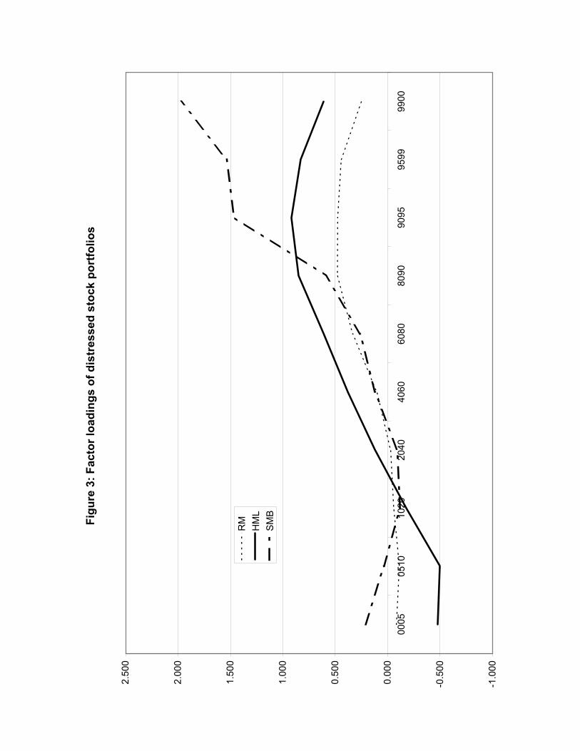
Figu

re 3

: Fac

tor l

oadi

ngs

of d

istr

esse

d st

ock

port

folio

s

-1.0

00

-0.5

00

0.00

0

0.50

0

1.00

0

1.50

0

2.00

0

2.50

0

0005

0510

1020

2040

4060

6080

8090

9095

9599

9900

RM

HM

LS

MB

Figu

re 4

: Ret

urns

on

long

-sho

rt d

istr

esse

d st

ock

port

folio

s

0110100

1000

1981

m1 1982

m1 1983

m1 1984

m1 1985

m1 1986

m1 1987

m1 1988

m1 1989

m1 1990

m1 1991

m1 1992

m1 1993

m1 1994

m1 1995

m1 1996

m1 1997

m1 1998

m1 1999

m1 2000

m1 2001

m1 2002

m1 2003

m1

$

LS10

90A

lpha

1090

Mar

ket r

etur

nLS

2080

Alp

ha20

80