1

Dynamic Evaluation of Corporate Distress Prediction Models

Mohammad Mahdi Mousavi*1,2, Jamal Ouenniche1

1Business School, University of Edinburgh, 29 Buccleuch Place, Edinburgh, UK, EH8 9JS

2Business School, Wenzhou Kean University, 88 Daxue Road, Wenzhou, China, 325060

Abstract: The design of reliable models to predict corporate distress is crucial as the likelihood of

filing for bankruptcy increases with the level and persistency of distress. Although a large number

of modelling and prediction frameworks for corporate failure and distress has been proposed, the

relative performance evaluation of competing prediction models remains an exercise that is mono-

criterion in nature, which leads to conflicting rankings of models. This methodological issue is

addressed by Mousavi et al (2015) by proposing an orientation-free super-efficiency data

envelopment analysis model as a multi-criteria assessment framework. This data envelopment

analysis (DEA) model is static in nature. In this research, we propose a dynamic DEA framework

to assess the relative performance of an exhaustive range of distress prediction models and rank

them accordingly. In addition, we address several research questions including how robust is the

out-of-sample performance of dynamic distress prediction models relative to static ones with

respect to sample type and sample period length? and to what extend the choice of distress

definition affects the ranking of competing prediction models before, during, and after an

important event?

Keywords: Corporate Failure Prediction; Bankruptcy; Performance Criteria; Performance

Measures; Data Envelopment Analysis; Dynamic DEA, Slacks-Based Measure

* Correspondence Author: s.m.m.mousavi@ed.ac.uk

2

1. Introduction

Predicting bankruptcy or corporate failure before it happens has such economic benefits for a range

of stakeholders (e.g., managers, investors, auditors, regulators) that a large number of prediction

models have been designed. In practice, managers could use distress prediction models as early

warning systems to take proper preventive actions against bankruptcy. From a conceptual point of

view, failure and distress predictions are classification problems, which use a number of features

– often extracted from accounting, market, or macroeconomic information – to classify firms into

one out of two or more risk categories. During the last decades, numerous studies have employed

different types of prediction models or methods from fields such as probability and statistics,

operations research, and artificial intelligence – for a detailed classification of distress prediction

models, we refer the reader to Aziz and Dar (2006), Bellovary et al. (2007) and Abdou and Pointon

(2011).

With the increasing number of prediction models, a strand of the literature has focused on assessing

the performance of these models and identifying the factors that drive performance such as

modelling frameworks, features selection, estimation methods, sampling, and performance criteria

and their measures (Zhou, 2013; Mousavi et al., 2015). As demonstrated by Mousavi et al. (2015),

the performance of prediction models is not only dependent on the nature of the modelling

frameworks and the type of features, but also on the performance evaluation process and the

underlying performance evaluation methodology (e.g., mono-criterion methodologies, multi-

criteria methodologies) and the performance criteria and measures with which it is fed. In fact,

recent comparative studies have compared the performance of competing failure prediction models

grounded into different modelling frameworks (e.g., Wu et al., 2010; Fedorova et al., 2013; Bauer

and Agarwal, 2014; Mousavi et al., 2015) and using alternative sampling techniques (e.g., Gilbert

et al., 1990; Neves and Vieira, 2006; Zhou, 2013), various features (e.g., Tinoco and Wilson, 2013;

Trujillo-Ponce et al., 2014; Mousavi et al., 2015), different feature selection procedures (e.g., Tsai,

2009; Unler and Murat, 2010) and a range of performance criteria (e.g., discriminatory power,

calibration accuracy, information content, correctness of categorical prediction) and their measures

along with different performance evaluation methodologies (Mousavi et al., 2015).

3

Our survey of the literature on comparative studies of failure prediction models revealed a variety

of shortcomings that prevent practitioners from an efficient ranking of models. As pointed out by

Bauer and Agarwal (2014), the literature on comparative studies suffers from two main drawbacks.

First, most of the existing studies failed to have a comprehensive comparison between all types of

prediction models; i.e., traditional statistical models, contingent claims analysis (CCA) models,

and survival analysis (SA) models. Second, the existing literature has used a restricted number of

criteria to evaluate the performance of competing models. To have a more comprehensive

comparative assessment, Bauer and Agarwal (2014) evaluated the performance of Taffler (1983),

Bharath and Shumway (2008) and Shumway (2001) as representative of the traditional statistical

models, CCA models and SA models, respectively. Further, they applied three types of criteria;

namely, discriminatory power, information content, and correctness of categorical prediction to

compare the performance of these models. On the other hand, Mousavi et al. (2015) emphasized a

methodological shortcoming in comparative studies arguing that although some studies consider

multiple criteria and related measures to compare competing models, the nature of the comparison

exercise remains mono-criterion, as they use a single measure of a single criterion at a time. The

drawback of this mono-criterion approach is that the rankings corresponding to different criteria

are often different (e.g., Bandyopadhyay, 2006; Theodossiou, 1991; Tinoco and Wilson, 2013),

which result in a situation where one cannot make an informed decision as to which model

performs best when taken all criteria into consideration. To overcome this methodological

drawback, Mousavi et al. (2015) proposed a multi-criteria assessment framework; namely, an

orientation-free super-efficiency data envelopment analysis. Finally, Zavgren (1983) argued that

most traditional failure and distress prediction models are based on the assumption that the

relationship between the dependent variable (e.g., probability of failure) and all independent

variables (e.g., accounting and market information) is stable over time. Empirical studies,

however, indicate that this stability is highly arguable (e.g., Charitou et al., 2004; du Jardin and

Séverin, 2012) and that the performance of models is sensitive to changes in macroeconomic

conditions (Mensah, 1984; Platt et al., 1994). For example, the logit model of Ohlson (1980)

performs better in the mid- to late 1980s, whereas the SA model of Shumway (2001) outperforms

other models in the 2000s. The changes in patterns of accounting- and market-based information

4

during time suggest that prediction models need to be re-estimated frequently to encompass the

most recent patterns of information (Grice and Ingram, 2001). In this research, we argue that

another shortcoming of the existing literature lies in the use of static performance evaluation

frameworks to compare prediction models, and we propose a dynamic multi-criteria performance

evaluation framework.

Recent studies have substituted financial distress for corporate failure in the implementation of

failure prediction models (e.g., Tinoco and Wilson, 2013; Geng et al., 2015; Wanke et al., 2015;

Laitinen and Suvas, 2016). Financial distress refers to the inability of a company to pay its financial

obligations as they mature (Beaver, 1966). Obviously, the financial situation of a distressed

company differs from a healthy one suggesting that, while a company moves toward deterioration,

its financial features shift towards the characteristics of failed firms. This movement towards

failure is a process that could take several time periods (e.g., years) and manifest itself through a

variety of signals, which could prevent failure, if predicted with a reasonable level of accuracy. In

this research, in addition to proposing new models to predict distress or detect its signals, we

propose a dynamic multi-criteria framework for assessing and monitoring the performance of

distress prediction models, which, as a by-product, allows one to detect signals of distress. To the

best of our knowledge, no previous research proposed a dynamic framework for the performance

evaluation and monitoring of prediction models. In practice, such a framework for the early

detection of signs of distress is both necessary and beneficial.

In this paper, we contribute to the academic literature in several respects. First, following the lead

of Xu and Ouenniche (2012) and Mousavi et al. (2015) who proposed static multi-criteria

frameworks for assessing the relative performance of prediction models, we propose a new

dynamic multi-criteria framework for assessing and monitoring the relative performance of

prediction models over time and ranking them. Second, we consider a more in-depth classification

of statistical distress prediction models and perform an exhaustive evaluation taking into account

the most popular models of each class. In sum, we assess the performance of univariate

discriminant analysis (UDA), multivariate discriminant analysis (MDA), linear probability

analysis (LPA), probit analysis (PA) and logit analysis (LA) models as traditional techniques;

5

Black-Scholes-Merton (BSM)-based models, naïve BSM-based models, and naïve down-and-out

call (DOC) barrier option models as contingent claims analysis (CCA) models; and duration

independent and duration dependent survival analysis (SA) models. To best of our knowledge, this

study is the first to propose the Cox model with time-varying variables using UK data for distress

prediction, or equivalently estimating distress probabilities. To date, this study provides the most

comprehensive empirical comparative analysis of statistical distress prediction models. Third, we

provide answers to several important research questions using a rolling horizon sampling

framework and a dynamic performance evaluation and monitoring framework: What category of

information or combination of categories of information enhances the predictive ability of models

best? and How the out-of-sample performance of dynamic distress prediction models compare to

the out-of-sample performance of static ones with respect to sample type and sample period

length?

The rest of the paper unfolds as follows. Section 2 reviews the literature on advances in and

comparative studies on distress prediction models. Section 3 describes the proposed dynamic

multi-criteria framework; namely, a non-oriented super-efficiency Malmquist DEA, for the

comparison of prediction models. Section 4 provides details on our experimental design including

data, sample selection, and the variety of distress prediction models compared as part of this study.

Section 5 summarises our empirical results and discusses our findings. Finally, section 6 concludes

the paper.

2. Comparative studies on distress prediction models

In this section, we provide a concise account of advances on distress prediction modeling (see

section 2.1) along with a detailed survey of comparative studies (see section 2.2).

2.1. Advances in distress prediction models

Failure and distress prediction models could be divided into several categories depending on the

choice of the classification criteria. In this paper, we focus on a variety of models but the artificial

intelligence and mathematical programming ones. In sum, we consider the first generation of

6

models; namely, discriminant analysis (DA) models (e.g., Beaver, 1966, 1968; Altman, 1968;

Deakin, 1972; Blum, 1974; Altman et al., 1977), the second generation of models; namely,

probability models such as linear probability (LP) models (e.g., Meyer and Pifer, 1970), logit

analysis (LA) models (e.g., Martin, 1977; Ohlson, 1980), and probit analysis (PA) models (e.g.,

Zmijewski, 1984), and the third generation of models; namely, survival analysis (SA) models (e.g.,

Lane et al., 1986; Crapp and Stevenson, 1987; Luoma and Laitinen, 1991; Shumway, 2001) and

contingent claims analysis (CCA) models (e.g., Hillegeist et al., 2004; Bharath and Shumway,

2008).

Beaver (1966, 1968) is the pioneering study which proposed a univariate discriminant analysis

model fed with financial ratios information to predict failure. However, the first multivariate study

was undertaken by Altman (1968) who estimated a score, commonly referred to as a “Z-score”, as

a proxy of the financial situation of a company using multivariate discriminant analysis (MDA).

The suggested MDA technique was frequently used in later studies (e.g., Deakin, 1972; Blum,

1974; Altman et al., 1977; Altman, 1983). The majority of subsequent studies applied the second

generation models; that is, linear probability models (e.g., Meyer and Pifer, 1970), logit models

(e.g., Martin, 1977; Ohlson, 1980), and probit models (e.g., Zmijewski, 1984). These first and

second generations of models could be viewed as empirical models in that they are driven by

practical considerations such as an accurate prediction of the risk class or an accurate estimate of

the probability of belonging to a risk class; in sum, the choice of the explanatory variables is driven

by the predictive performance of the models. These models and their usage in some previous

studies are not without limitations. In fact, some of the assumptions underlying the modelling

frameworks may not be reasonably satisfied for some datasets, on one hand, and earliest studies

restricted the type of information to accounting-based one. In addition, these models are static in

nature and therefore fail to properly account of changes over time in the profiles of companies.

The third generation of models; namely, survival analysis (SA) models and contingent claims

analysis (CCA) models overcome some of these issues. In fact, the underlying modelling

frameworks of both SA models and CCA models are dynamic by design. In addition, most

previous studies made use of additional sources of information to enhance the performance of

these models; namely, market-based information (e.g., Hillegeist et al., 2004; Bharath and

7

Shumway, 2008) and macroeconomic information (e.g., Tinoco and Wilson, 2013; Kim and

Partington, 2014; Charalambakis and Garrett, 2015) although one might argue that the

approximation process of unobservable variables (e.g., volatility, expected return, market value of

assets) is not free of potential measurement errors (Aktug, 2014). To be more specific, SA models

are used to estimate time-varying probabilities of failure. Despite the application of SA models in

failure prediction dates back to the mid-1980s (e.g., Lane et al., 1986; Crapp and Stevenson, 1987;

Luoma and Laitinen, 1991), Shumway (2001) was the pioneering study which made its use popular

by providing an attractive estimation methodology based on an equivalence between multi-period

logit models and a discrete-time hazard model. Thereafter, the suggested discrete-time hazard

model – also referred to as a discrete-time logit model – was frequently used in later studies (e.g.,

Chava and Jarrow, 2004; Wu et al., 2010; Tinoco and Wilson, 2013; Bauer and Agarwal, 2014) to

estimate the coefficients of time-varying accounting and market-based covariates of SA models.

Unlike, the first generation models, the second generation models, and SA models, which are

empirical models, CCA models – also referred to as Black-Scholes-Merton (BSM)-based models

– are theoretically grounded. In fact, these models are grounded into option-pricing theory, as set

out in Black and Scholes (1973) and Merton (1974) whereby the equity holders’ position in a firm

is assumed to be the long position in a call option. Therefore, as suggested by McDonald (2002),

the probability of failure could be interpreted as the likelihood that the value of firm’s assets will

be less than the face value of firm’s liabilities at maturity; i.e., the call option expires worthless.

These models make use of market-based information by incorporating company stock returns and

their volatility in estimating the probability of failure (Hillegeist et al., 2004; Bharath and

Shumway, 2008). Like any modelling framework, CCA models are not without their limitations.

For example, CCA models implicitly assume that the liabilities of the firm have the same

maturities, which in practice is a limitation (Saunders and Allen, 2002).

2.2. Comparative studies of failure prediction models

This section provides a survey on the studies, which focus on the comparison of different types of

failure or distress prediction models; namely, the first generation of models, the second generation

of models, and the third generation of models. Our survey focus is on models and performance

8

criteria and their measures, which have been applied by the existing literature on the evaluation of

competing prediction models.

Comparison between first and second generation models: Before the breakthrough model of

Shumway (2001), the first and second generations of models were the prevailing techniques in

classification. Since the implementation of DA in failure prediction by Beaver (1966) and Altman

(1968) to the early 1980s, MDA was the superior method for predicting corporate failure. In fact,

ease of use and interpretation were the main reasons of the popularity of DA. However, the validity

of these models depends on the extent to which the underlying assumptions (i.e., multivariate

normality, equal groups’ variance-covariate matrices) hold in a dataset. From the 1980s to 2001,

LA models (introduced by Ohlson, 1980) and PA models (introduced by Zmijewski, 1984) became

the prevailing techniques. Despite the fact that probability models are more attractive from a

practical perspective in that the underlying assumptions are less restrictive, most comparative

studies have indicated that the prediction powers of LA models and PA models are similar to those

of DA models (e.g., Press and Wilson, 1978; Collins and Green, 1982; Lo, 1986). A notable

exception is Lennox (1999) who suggested that well-specified probit and logit models outperform

DA models.

Comparison between first and second-generation models and survival analysis models: From a

conceptual perspective, SA models are superior to discriminant analysis models and probability

models, because of their dynamic nature. However, empirical results across several comparative

analyses seem to report mixed findings. From an empirical perspective, the features of a modelling

framework design that are not being fully supported or exploited by the dataset under consideration

nullify its conceptual advantage. In sum, the choice combination of a modelling framework and

the features to feed into it has a more significant role in enhancing or downgrading prediction

performance.

For example, Luoma and Laitinen (1991) compared the performance of a semiparametric Cox

hazard model with a DA model and an LA model – all models fed with accounting based

information – with respect to type I and type II errors as measures of correctness of categorical

prediction. The results suggested that the developed SA was inferior to both DA and LA models

9

with respect to type I and type II errors. Further, their research was limited with respect to the

number of criteria, since they only used correctness of categorical prediction.

Shumway (2001) proposed a discrete-time SA model – using a multi-period logit estimation

technique – for failure prediction and compared its performance with the performance of DA, LA

and PA using overall correct classification rate (OCC) as a measure of correctness of categorical

prediction. The results indicate that an SA model, which encompasses both accounting and market

information (respectively, only accounting information) outperforms (respectively,

underperforms) DA, LA and PA models. However, with respect to the choice of performance

criteria and their measures, this study is also restricted to correctness of categorical prediction as

a criterion and overall accuracy – also known as overall correct classification rate – as its measure.

Comparison between first and second generation models and contingent claims models; Hilligeist

et al. (2004) compared the performance of an BSM-based model with two types of representative

models of the first and second generation of models; namely, MDA and LA models (Altman, 1968;

Ohlson, 1980), respectively. They used Log-Likelihood and Pseudo-R2 as measures of information

content to evaluate the performance of these models. The results suggested that the BSM-based

model outperforms both the original and the refitted versions of Altman (1968) and Ohlson (1980)

models on information content. Furthermore, they found out that the original Altman (1968) with

coefficients estimated with a small data set from decades earlier outperformed the refitted one with

updated coefficients using recent data suggesting that refitting models with more recent data does

not necessarily improve performance. However, this study is restricted to one criterion; i.e.,

information content, for comparing the performance of models.

Reisz and Perlich (2007) compared the performance of three contingent claims models; namely, a

BSM model, a KMV model developed by KMV Corporation in 1993 and then acquired by

Moody's Corporation in 2002, and a Down-and-Out Call option (DOC) model, with the MDA

model of Altman (1968). Recall that the KMV model – also referred to as the Expected Default

Frequency (EDF) model – is actually a four-step procedure based on Merton’s framework, which

determines a default point, estimates asset value and volatility, computes distance to default (DD),

and converts DD into expected default frequency (EDF). They use ROC as a measure of

10

discriminatory power and Log-Likelihood as a measure of information content. They found out

that the DOC model outperforms the other types of contingent claims models as well as MDA for

3-, 5- and 10-year ahead failure prediction. Unexpectedly, Altman (1968) outperforms all

contingent claims models for 1-year ahead failure prediction. Although this study encompassed

two types of criteria; i.e., discriminatory power and information content, the comparison is

somehow incomplete as the log-likelihood cannot be computed for Altman’s model.

Agarwal and Taffler (2008) compared the performance of two types of BSM models; namely,

Hillegeist et al. (2004) and Bharath and Shumway (2008), with the MDA model of Taffler (1983)

with respect to ROC as a measure of discriminatory power, Log-likelihood and Pseudo-R2 as

measures of information content, and return on assets (ROA) and return on risk weighted assets

(RORWA) as measures of economic value, given different costs of misclassification. The

empirical results showed that the MDA model outperforms Hillegeist et al. (2004) significantly on

ROC as a measure of discriminatory power. Meanwhile, MDA model does not outperform Bharath

and Shumway (2008) significantly on ROC. On the other hand, with respect to Log-likelihood as

a measure of information content, Hillegeist et al. (2004) performs significantly better than Bharath

and Shumway (2008) and MDA model, respectively. However, Pseudo-R2 was higher for Taffler

(1983) compared to BSM models, which suggests that these two information content measures

carry different elements of information. Furthermore, taking into account differences in

misclassification costs, they compared the economic benefit of applying Bharath and Shumway

(2008) or Taffler (1983) as classifiers using the approach proposed by Blochlinger and Leippold

(2006). The results suggest that the MDA model of Taffler (1983) outperforms BSM-based

models. It is worth to mention that with respect to the number of criteria, this study was innovative

in its era since three criteria; namely, the correctness of categorical prediction, discriminatory

power and information content, were used for evaluating models.

Comparison between contingent claims models and survival analysis models: Campbell et

al.(2008) proposed a duration-dependent SA model and evaluated its performance with the

performances of a KMV model and the duration-independent SA model of Shumway (2001) using

log-likelihood and pseudo-R2 as measures of information content. The results indicate that their

11

SA model outperforms both the SA model of Shumway (2001) and the KMV model. However,

this study fails to incorporate more criteria for comparing the performance of models.

Comparison between first, second and third generations of models: Wu et al. (2010) compared the

performance of the MDA model of Altman (1968), the LA model of Ohlson (1980), the PA model

of Zmijewski (1984), the duration-independent SA model of Shumway (2001) and the BSM model

of Hillegeist et al. (2004). The results indicate that, with respect to Log-likelihood and Pseudo-R2

as measures of information content, the discrete time SA model of Shumway outperforms LA, PA,

BSM and MDA models, respectively. Unexpectedly, with respect to overall correct classification

rate as a measure of correctness of categorical prediction, Ohlson model of LA outperforms MDA,

PA, BSM, SA models, respectively, under a rolling window implementation. For ROC as a

measure of discriminatory power, the authors failed to take account of BSM model, the result

suggest that the duration-independent SA model of Shumway performs better than LA, MDA, and

PA, respectively. Referring to the number of criteria, this study puts comparison into effect with

three types of criteria, namely, the correctness of categorical prediction, discriminatory power, and

information content.

To conclude this section, we would like to refer the reader to Appendix A for a summary table of

the literature on comparative analyses of failure models. We also refer the reader to Appendix C

of Mousavi et al (2015) for a sample of typical performance criteria and their measures used in

assessing failure prediction models.

3. A Dynamic Framework for Assessing Distress Prediction Models: Non-Oriented Super-

Efficiency Malmquist DEA

Malmquist productivity index is a multi-criteria assessment framework for performing

performance comparisons of DMUs over time. Fare et al. (1992, 1994) employed DEA to extend

the original Malmquist (1953) and construct the DEA-based Malmquist productivity index as the

product of two components, one measuring the efficiency change (EC) of DMU with respect to

the efficiency possibilities defined by the frontier in each period (also referred to as caching-up to

12

the frontier), and the other measuring the efficient frontier-shift (EFS) between the two time

periods 𝑡 and 𝑡 + 1 (also referred to as change in the technical efficiency evaluation).

Figure 1: Efficiency Change and Efficient Frontier-Shift

Let 𝑥𝑖0𝑡 denote the 𝑖th input and 𝑦𝑟0

𝑡 denote the 𝑟th output for 𝐷𝑀𝑈0, both at period 𝑡. The Figure

1 shows the change of efficiency of 𝐷𝑈𝑀0 from point 𝐴 (with respect to efficient frontier at period

𝑡) to point 𝐵 (with respect to efficient frontier at period 𝑡 + 1) assuming to have one input and one

output. The efficiency change (𝐸𝐶) component is measured by the following formula:

EC =

𝑃𝐹𝑃𝐵⁄

𝑄𝐶𝑄𝐴⁄

=Efficiency of DMU0 with respect to the period 𝑡 + 1

Efficiency of DMU0 with respect to the period 𝑡

(1)

Let Δ𝑡2((𝑥0, 𝑦0)𝑡1) denote the efficiency score of DUM with 𝑥0 input and 𝑦0 output at period 𝑡1

(say, 𝐷𝑀𝑈(𝑥0, 𝑦0)𝑡1) relative to frontier 𝑡2. Replacing 𝑡1 and 𝑡2 with 𝑡 and 𝑡 + 1, respectively, the

𝐸𝐶 effect (say, 𝛼) can be presented as:

𝐸𝐶: 𝛼 =Δ𝑡+1((𝑥0, 𝑦0)𝑡+1 )

Δ𝑡((𝑥0, 𝑦0)𝑡) (2)

Thus, 𝐸𝐶 > 1 shows an improvement in relative efficiency from period 𝑡 to 𝑡 + 1, while 𝐸𝐶 =

1 and 𝐸𝐶 < 1 shows stability and deterioration in relative efficiency, respectively.

13

Also, Figure 1 indicates that the reference point of (𝑥0𝑡 , 𝑦0

𝑡) moved from C on the frontier of period

𝑡 to D on the frontier of period 𝑡 + 1. Therefore, the efficient frontier-shift (EFS) effect at (𝑥0𝑡 , 𝑦0

𝑡)

is equivalent to:

𝐸𝐹𝑆𝑡 =𝑄𝐶

𝑄𝐷=

𝑄𝐶𝑄𝐴⁄

𝑄𝐷𝑄𝐴⁄

=Efficiency of (x0

t , y0t ) with respect of the period t frontier

Efficiency of (x0t , y0

t ) with respect of the period t + 1 frontier

(3)

Similarly, the 𝐸𝐹𝑆 effect at (𝑥0𝑡+1, 𝑦0

𝑡+1) is equivalent to:

𝐸𝐹𝑆𝑡+1 =𝐵𝐹

𝐵𝐷=

𝐵𝐹𝐵𝑄⁄

𝐵𝐷𝐵𝑄⁄

=Efficiency of (x0

t+1, y0t+1)with respect of the period t frontier

Efficiency of (x0t+1, y0

t+1)with respect of the period t + 1 frontier

(4)

The EFS component is measured by the geometric mean of EFS effect at (𝑥0𝑡 , 𝑦0

𝑡) (say,

𝐸𝐹𝑆𝑡) and EFS effect at (𝑥0𝑡+1, 𝑦0

𝑡+1) (say, 𝐸𝐹𝑆𝑡+1);

𝐸𝐹𝑆 = [𝐸𝐹𝑆𝑡 × 𝐸𝐹𝑆𝑡+1]1

2⁄ (5)

Using our notation, the EFS effect can be expressed as:

𝐸𝐹𝑆: 𝛽 = [Δ𝑡((𝑥0, 𝑦0)𝑡)

Δ𝑡+1((𝑥0, 𝑦0)𝑡)×

Δ𝑡((𝑥0, 𝑦0)𝑡+1)

Δ𝑡+1((𝑥0, 𝑦0)𝑡+1)]

1/2

(6)

Therefore, the Malmquist Productivity index (MPI) can be written as;

𝑀𝑃𝐼 = 𝐸𝐶 × 𝐸𝐹𝑆 (7)

Using our notation, the MPI can be presented as:

14

𝑀𝑃𝐼: 𝛾 = 𝛼 × 𝛽

=Δ𝑡+1((𝑥0, 𝑦)𝑡+1 )

Δ𝑡((𝑥0, 𝑦0)𝑡)

× [Δ𝑡((𝑥0, 𝑦0)𝑡)

Δ𝑡+1((𝑥0, 𝑦0)𝑡)×

Δ𝑡((𝑥0, 𝑦0)𝑡+1)

Δ𝑡+1((𝑥0, 𝑦0)𝑡+1)]

1/2

(8)

MPI could be rearranged as;

𝛾 = [Δ𝑡((𝑥0, 𝑦0)𝑡+1)

Δ𝑡((𝑥0, 𝑦0)𝑡)×

Δ𝑡+1((𝑥0, 𝑦0)𝑡+1)

Δ𝑡+1((𝑥0, 𝑦0)𝑡)]

1/2

(9)

This explanation of MPI could be interpreted as the geometric mean of efficiency change measured

by period 𝑡 and 𝑡 + 1 technology, respectively. 𝑀𝑃𝐼 > 1 shows an improvement in the total factor

productivity of 𝐷𝑀𝑈0 from period 𝑡 to 𝑡 + 1 , while 𝑀𝑃𝐼 = 1 and 𝑀𝑃𝐼 < 1 shows stability and

deterioration in total factor productivity, respectively.

Comment 1: Caves et al. (1982) introduced a distance function, Δ(. ), to measure technical

efficiency in the basic CCR model (Charnes et al., 1978). Though, in the non-parametric

framework, instead of using a distance function, DEA models are implemented. For example, Fare

et al. (1994) used input (or output) oriented radial DEA to measure the MPI. However, the radial

model faces a lack of attention to slacks, which could be overcome using Slack-based non-radial

oriented (or non-oriented) DEA model (Tone, 2001, 2002).

In this study, we use the non-radial (slack-based measure), non-oriented super- efficiency DEA

(Tone, 2002, 2001) Malmquist index to evaluate the performance of competing distress prediction

models. The reason to choose an orientation-free evaluation is that we aim to evaluate distress

prediction models, and thus, the choice between input-oriented or output-oriented analysis is

irrelevant. Further, our study is under variable return to scale (VRS) assumption, where input-

oriented and output-oriented analysis may result in different scores and rankings of DMUs. On the

other hand, the reason to choose non-radial framework is that, radial DEA models may be

infeasible for some DMUs; therefore, ties would stay in rankings. Moreover, radial DEA models

15

overlook possible slacks in inputs and outputs, and therefore, would possibly over-estimate the

efficiency scores by ignoring mix efficiency.

Further, basic DEA techniques cannot distinguish between efficiency DMUs (here, distress

prediction models) because all their scores are equal to 1 (Anderson and Peterson, 1993).

Therefore, we choose super-efficiency DEA framework, as we are interested in acquiring a

complete ranking of distress prediction models.

Considering the production possibility set 𝑃 defined by Cooper et al. (2006) as

𝑃 = {(𝑥, 𝑦)|𝑥 ≥ 𝑋𝑡1𝜆, 𝑦 ≤ 𝑌𝑡1𝜆, 1 ≤ 𝑒𝜆 ≤ 1, 𝜆 ≥ 0}, (10)

SBM-DEA (Tone, 2001) measures the efficiency of DMU (𝑥0, 𝑦0)𝑡2 (𝑡2 = 1,2) with respect to

the benchmark set (𝑋, 𝑌)𝑡1(𝑡1 = 1,2) using the following linear programing (LP):

Δ𝑡1((𝑥0, 𝑦0)𝑡2) = min𝜆,𝑠−,𝑠+

1 −1𝑚

∑𝑠𝑖

−

𝑥𝑖𝑜𝑡2

𝑚𝑖=1

1 +1𝑟

∑𝑠𝑖

+

𝑦𝑖𝑜𝑡2

𝑟𝑖=1

subject to 𝑥𝑜𝑡2 = 𝑋𝑡1𝜆 + 𝑠−,

𝑦0𝑡2 = 𝑌𝑡1𝜆 − 𝑠+ ,

1 ≤ 𝑒𝜆 ≤ 1, 𝜆 ≥ 0, 𝑠− ≥ 0, 𝑠+ ≥ 0.

(11)

where Δ𝑡1((𝑥0, 𝑦0)𝑡2) is the efficiency score of 𝐷𝑀𝑈(𝑥0, 𝑦0)𝑡1 relative to frontier 𝑡2; 𝑋𝑡1 =

(𝑥1𝑡1 , … , 𝑥𝑛

𝑡1) ∈ ℝ𝑛 and 𝑌𝑡1 = (𝑦1𝑡1 , … , 𝑦𝑛

𝑡1) ∈ ℝ𝑛 are matrices of inputs and outputs at the period

𝑡1, respectively; 𝑠− ≥ 0 and 𝑠+ ≥ 0 are the vectors of input surpluses and output shortages in ℝ𝑛,

respectively, and are named slacks; 𝑒 is a row vector with all items equal to one, and 𝜆 is a

nonnegative vector in ℝ𝑛.

Or equivalently;

Δ𝑡1((𝑥0, 𝑦0)𝑡2) = min𝜃,𝜂,𝜆

1𝑚

∑ 𝜃𝑖𝑚𝑖=1

1𝑟

∑ 𝜂𝑖𝑟𝑖=1

(12)

16

subject to 𝜃𝑖𝑥𝑖𝑜𝑡2 ≥ ∑ 𝑥𝑖𝑗

𝑡1𝑛

𝑗=1𝜆𝑗 (𝑖 = 1, … , 𝑚),

𝜂𝑖𝑥𝑖𝑜𝑡2 ≥ ∑ 𝑦𝑖𝑗

𝑡1𝑛

𝑗=1𝜆𝑗 (𝑖 = 1, … , 𝑟) ,

𝜃𝑖 ≤ 1(𝑖 = 1, … , 𝑚), 𝜂𝑖 ≥ 1(𝑖 = 1, … , 𝑟), 1 ≤ 𝑒𝜆 ≤ 1,

𝜆 ≥ 0.

where 𝜃𝑖and 𝜂𝑖 are (1 −𝑠𝑖

−

𝑥𝑖𝑜𝑡2

) and (1 +𝑠𝑖

+

𝑦𝑖𝑜𝑡2

), respectively.

Referring to equation 9, someone can use equation 11 to estimated Δ0𝑡 (𝑥0

𝑡 , 𝑦0𝑡), Δ0

𝑡+1(𝑥0𝑡+1, 𝑦0

𝑡+1),

Δ0𝑡 (𝑥0

𝑡+1, 𝑦0𝑡+1) and Δ0

𝑡+1(𝑥0𝑡 , 𝑦0

𝑡) as four required terms for calculating MPI.

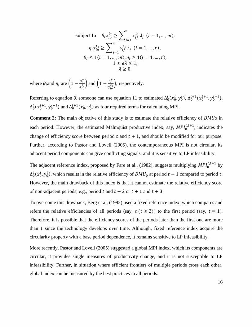
Comment 2: The main objective of this study is to estimate the relative efficiency of 𝐷𝑀𝑈𝑠 in

each period. However, the estimated Malmquist productive index, say, 𝑀𝑃𝐼0𝑡,𝑡+1

, indicates the

change of efficiency score between period 𝑡 and 𝑡 + 1, and should be modified for our purpose.

Further, according to Pastor and Lovell (2005), the contemporaneous MPI is not circular, its

adjacent period components can give conflicting signals, and it is sensitive to LP infeasibility.

The adjacent reference index, proposed by Fare et al., (1982), suggests multiplying 𝑀𝑃𝐼0𝑡,𝑡+1

by

Δ0𝑡 (𝑥0

𝑡 , 𝑦0𝑡), which results in the relative efficiency of 𝐷𝑀𝑈0 at period 𝑡 + 1 compared to period 𝑡.

However, the main drawback of this index is that it cannot estimate the relative efficiency score

of non-adjacent periods, e.g., period 𝑡 and 𝑡 + 2 or 𝑡 + 1 and 𝑡 + 3.

To overcome this drawback, Berg et al, (1992) used a fixed reference index, which compares and

refers the relative efficiencies of all periods (say, 𝑡 (𝑡 ≥ 2)) to the first period (say, 𝑡 = 1).

Therefore, it is possible that the efficiency scores of the periods later than the first one are more

than 1 since the technology develops over time. Although, fixed reference index acquire the

circularity property with a base period dependence, it remains sensitive to LP infeasibility.

More recently, Pastor and Lovell (2005) suggested a global MPI index, which its components are

circular, it provides single measures of productivity change, and it is not susceptible to LP

infeasibility. Further, in situation where efficient frontiers of multiple periods cross each other,

global index can be measured by the best practices in all periods.

17

Figure 2: Global Frontier

As Figure 2 presents, the relative efficiency of 𝐷𝑀𝑈0 can be measured in terms of either the

frontier of period 1 (consists of four DMUs of 1,2,3,4 and 5) or the frontier of period 2 (consist of

four DMUs of 6,7,8,9 and 10). An alternative is the global frontier, which is the combination of

the best DMUs in the history, i.e. five DMUs of 6,7,3,4 and 5.

It is argued that if the length of observation period is long enough, the current DMUs would be

covered by the best historical DMUs, probably themselves. As a result, the relative efficiency to

the global frontier could be considered as an absolute efficiency with the scores less than or equal

to 1 (Pastor and Lovell, 2005).

4. Empirical investigation

In this section, we provide the details of our empirical investigation, where we compare the

performance of both existing and new distress prediction models using both mono- and multi-

criteria performance evaluation frameworks. In the remainder of this section, we shall provide

details on our dataset (see section 4.1), features selection (see section 4.2), sampling and fitting

choices (see section 4.3), distress prediction models (see section 4.4), and our empirical results

and findings (see section 4.5).

18

4.1. Data

The dataset used in our empirical analysis is chosen as follows. First, we considered all non-

financial and non-utility UK companies listed on the London Stock Exchange (LSE) at any time

during a 25-year period from 1990 through 2014. Second, since only post-listing information is

used as input to our prediction models and these models have minimum historical data

requirements, we excluded companies that have been listed for less than 2 years.

In all databases, there are several companies with missing data. Our dataset is no exception.

Excluding those companies with missing data is a source of potential error in evaluating prediction

models (Zmijewski, 1984; Platt and Platt, 2012). Therefore, in order to minimise any bias related

to this aspect, we only excluded those companies with missing values for the main accounting

book items (e.g., sales, total assets) and market information (e.g., price) which are required for

computing many accounting and market-based ratios (Lyandres and Zhdanov, 2013). The

remaining companies with missing values were dealt with by replacing the missing values for each

company by its most recently observed ones (Zhou et al., 2012).

As to outlier values amongst the observed variables, we winsorized these variables; that is, we sat

the values lower (respectively, greater) than the 1st (respectively, 99th) percentile of each variable

equal to that value (Shumway, 2001).

With respect to the definition of distress, we considered the proposed definition by Pindado et al.

(2008). The distress definition is represented by a binary variable, say 𝐷, equals 1 for financially

distressed companies and equals 0 otherwise, where a company is considered financially distressed

if it meets both of the following conditions: (1) its earnings before interest, taxes, depreciation and

amortization (EBITDA) is lower than its interest expenses for two consecutive years, and (2) the

company experience negative growth in market value for two consecutive years. Details on the

number of companies in our dataset and their distress status are provided in Table 2. Notice that

the legal aspects of distress complement the financial ones, which strengthens the overall definition

of distress given that a relatively low proportion of companies fall under code 21.

19

Table 1: Basic Sample Statistics This table presents the total number of distressed companies versus healthy ones

for the period of 1990 and 2014.

Observation (1990-2014) # %

Distressed company-year observations (𝐷) 1414 3.82%

Healthy company-year observations 35,570 96.18%

Total company-year Observation 36,984 100%

In sum, our dataset consists of 3,389 companies and 36,984 company-year observations. Among

the total number of observation, there are 1,414 company-year observations classified as distressed

resulting in a distress rate average of 3.82% per year.

Figure 3 displays the market value of LSE as measured by the FTSE-all index, the average of

financial distress and failure rate during 25 years from 1990 through 2014. This graphical snapshot

clearly highlights the consistency between our chosen definitions of distress. In addition, the

percentage of failed companies as well as our distress variables expressed in percentage terms and

the performance of the UK stock market are, as one would expect, inversely moving together in a

consistent fashion, which suggest that the use of market information would in principle enhance

distress prediction.

Figure 3: Financial distress rate and market value of LSE trend

4.2. Feature Selection

There is a variety of strategies and methods for identifying the most effective group of features to

feed failure prediction models with (Balcaen and Ooghe, 2006). Feature selection strategies could

0

500000

1000000

1500000

2000000

2500000

0.00%

2.00%

4.00%

6.00%

8.00%

10.00%

12.00%

14.00%

1990 1992 1994 1996 1998 2000 2002 2004 2006 2008 2010 2012 2014

Mar

ket

val

ue

of

FT

SE

AL

L (

£ M

ill)

Fai

lure

& D

istr

ess

rate

Bktcy_Rate Dist_Rate FTSEALL_MV

20

be theoretically grounded, empirically grounded, or both – see, for example, Laitinen and Suvara

(2016). On the other hand, feature selection methods could be objective or subjective. Objective

feature selection methods could be statistical (e.g., Tsai, 2009; Zhou et al., 2012) or non-statistical

(e.g., Pacheco et al., 2007, 2009; Unler and Murat, 2010) but adopt a common approach; that is,

optimizing an effectiveness criterion. Whereas subjective feature selection methods make often

use of a subjective decision rule including reviewing the literature and selecting the most

commonly used features (e.g., Ravi Kumar and Ravi, 2007; Zhou, 2013, 2014; du Jardin, 2015;

Cleary and Hebb, 2016). In this research, we used a statistical objective feature selection method.

To be more specific, we reduced our very large initial set of accounting-based ratios (i.e., 83

accounting-based ratios) to 31 accounting-based features using factor analysis, where factors are

selected so that both the absolute values of their loadings are greater than 0.5 and their communities

are greater than 0.8, and the stopping criterion is either no improvement in the total explained

variance or no more variables are excluded. This factor analysis was run using principal component

analysis with VARIMAX as a factor extraction method (Chen, 2011; Mousavi et al., 2015).

4.3. Sample Selection

Following the lead of Mousavi et al. (2015), we test the performance of distress prediction models

out-of-sample; however, in this paper out-of-sample testing is implemented within a rolling

horizon framework. The aim here is to find out how robust is the out-of-sample performance of

dynamic distress prediction models relative to static ones with respect to sample type (i.e., pre-

crisis, crisis period, post-crisis) and sample period length. In our empirical investigation, we

considered three sample period lengths; namely, 3, 5, and 10 years. In sum, we use firm-year

observations from year 𝑡 − 𝑛 + 1 to year 𝑡 (𝑛 = 3,5,10) as a training sample to fit models; that is,

estimate their coefficient. Then, we use the fitted models to predict distress in year 𝑡 + 1. For the

sake of comparing the predictive ability of different models for different samples and different

sample period lengths, we are concerned with predicting distress from 2000 onwards; that is, 𝑡 =

1999 to 2013. The reader is referred to Figure 4 for a graphical representation of this process. The

details about the proportion of distressed firms for each training and holdout sample are presented

in Table 2.

21

Table 2 : The proportion of distress firms (𝐷) in training and holdout samples

This table presents the yearly proportion of distress in our training and hold-out samples. The proportion

of distress is presented based on definition of distress (𝐷) and three different length of training period.

Hold out

sample

3-year training

sample

5-year training

sample

10-year training

sample

Year D % Years D % Years D % Years D %

2000 1.60% 1997-1999 2.32% 1995-1999 1.79% 1990-1999 2.04%

2001 1.39% 1998-2000 2.32% 1996-2000 1.96% 1991-2000 2.11%

2002 6.22% 1999-2001 2.15% 1997-2001 1.99% 1992-2001 1.97%

2003 11.78% 2000-2002 3.04% 1998-2002 2.89% 1993-2002 2.23%

2004 3.21% 2001-2003 6.42% 1999-2003 4.82% 1994-2003 3.09%

2005 2.00% 2002-2004 6.97% 2000-2004 4.77% 1995-2004 3.29%

2006 3.06% 2003-2005 5.37% 2001-2005 4.76% 1996-2005 3.38%

2007 4.25% 2004-2006 2.75% 2002-2006 4.99% 1997-2006 3.54%

2008 5.86% 2005-2007 3.13% 2003-2007 4.62% 1998-2007 3.81%

2009 10.18% 2006-2008 4.37% 2004-2008 3.69% 1999-2008 4.21%

2010 4.15% 2007-2009 6.59% 2005-2009 4.94% 2000-2009 4.86%

2011 1.96% 2008-2010 6.77% 2006-2010 5.41% 2001-2010 5.10%

2012 5.21% 2009-2011 5.66% 2007-2011 5.37% 2002-2011 5.18%

2013 8.12% 2010-2012 3.76% 2008-2012 5.63% 2003-2012 5.09%

2014 5.56% 2011-2013 4.99% 2009-2013 6.01% 2004-2013 4.71%

Figure 4: Rolling window periodic sampling

22

4.4. Distress Prediction Models for Comparative Study

The academic literature includes a broad number of FPMs, which have been employing to predict

corporate failure. As mentioned earlier, generally, FPMs could be classified into two main

categories; namely, statistical models and non-statistical models. The focus of this study is on

statistical models, which could be classified into two sub-categories, namely, static and dynamic

models. The selection choice of static models in our comparative analysis is based on two factors;

the pioneering proposed static frameworks, and the most frequent applied frameworks in other

comparative studies. Further, the selection choice of dynamic models is based on two criteria; the

most frequent applied dynamic frameworks in other comparative studies and the recent proposed

dynamic frameworks in the literature. As a result of mentioned criteria, we end up with four static

frameworks (i.e., univariate discriminant analysis, multivariate discriminant analysis, logit

analysis, probit analysis), and four dynamic frameworks (i.e., contingent claim analysis (CCA)

models, duration independent hazard models without time-invariant baseline, duration

independent hazard with time invariant baseline and duration dependent hazard with time variant

baseline).

To be more specific, the traditional accounting based models considered in our comparative study

include the univariate discriminant analysis (UDA) model proposed by Beaver (1966); the MDA

models proposed by Altman (1968), Altman (1983), Taffler (1983) and Lis (1972); the logit model

proposed by Ohlson (1980); the probit model proposed by Zmijewski (1984); and, the linear

probability model propose by Theodossiou (1991). The dynamic models considered in our study

include; BSM-based models proposed by Hillegeist et al. (2004) and Bharath, Shumway (2008)

and the naïve down-and-out call (DOC) barrier option model proposed by Jackson and Wood

(2013), duration-independent hazard model with time-invariant baseline proposed by Shumway

(2001), duration-independent hazard model without time-invariant baseline model, and duration-

dependent with time-variant baseline proposed by Kim and Partington (2014).

23

4.4.1. Traditional statistical techniques

4.4.1.1. Discriminant analysis (DA)

DA was firstly proposed by Fisher (1938) to classify an observation into two or several a priori

categories dependent upon the observation’s individual features. The initial objective of DA is to

minimize within-group distance and maximize between-group distance (also, referred as

Mahalanobis distance). Assuming there are 𝑛 groups, the generic form of DA model for the group

𝑘 could be shown as follows;

𝑧𝑘 = 𝑓 (∑ 𝛽𝑘𝑗𝑥𝑗

𝑝

𝑗=1

) (13)

where 𝑥𝑗 is the discriminant features 𝑗, 𝛽𝑘𝑗 is the discriminant coefficients of group 𝑘 for

discriminant feature 𝑗, 𝑧𝑘 represents the score of group 𝑘, and is the linear or non-linear

classifier that maps the scores, say onto a set of real numbers. Note that to compare DA models

to other statistical models, we need to estimate the probability of failure, which is used as an input

for estimating many measures of performance. For this, we follow Hillegeist et al. (2004) in using

a logit link to calculate the probability of failure for companies;

𝑃(𝑓𝑎𝑖𝑙𝑢𝑟𝑒)𝑖 =𝑒𝑧

1 + 𝑒𝑧 (14)

The main shortcoming of DA is that its suitability in optimal discrimination between groups rests

on satisfying two underlying assumptions, i.e., the joint normal distribution of features and equal

group variance-covariance matrices (Collins and Green, 1982). Although, in practice, the features

are rarely normally distributed (Eisenbeis, 1977; Mcleay, 1986) and the groups are hardly equal in

variance-covariance matrices (Hamer, 1983), the robustness of DA against deviation from these

assumptions for optimality, makes it a widely used method of classification (du Jardin and Séverin,

2012). In this study, we examine the UDA model proposed by Beaver (1966); the MDA models

proposed by Altman (1968), Altman (1983), Altman et al. (1995), Taffler (1983) and Lis (1972).

f

xt

24

4.4.1.2. Regression Models

The linear probability model (LPM), introduced by Meyer and Pifer (1970) in failure prediction,

is a special case of OLS regression when the dependent variable is dichotomous. Similar to OLS,

LPM assumes the linear relationship as 𝑌 = 𝑋𝛽 + 𝜖; where 𝑌 is an 𝑁 × 1 vector of dependent

variable, 𝑋 is an 𝑁 × 𝐾 matrix of independent variables (features), and, 𝜖 is an 𝑁 × 1 vector of

error terms with 𝐸(𝜖) = 0. Generally, in case of failure prediction, 𝑌 is a Bernoulli random

variable (say, 𝑌 equals 1 or 0) and by its very nature two corresponding likelihood, say probability

of failure (𝑃) where 𝑌𝑖 = 1 and probability of non-failure (1 − 𝑃) where 𝑌𝑖 = 0 are apparent.

Given 𝑃 and 1 − 𝑃 and binary values of 𝑌, then 𝐸(𝑌𝑖) = 1(𝑃) + 0(1 − 𝑃) which indicates

that 𝑋𝛽 = 𝑃.

One of the major shortcomings of LPM is that 𝜖, which equals to 𝑌 − 𝑋𝛽, could be either 1 − 𝛽𝑋

(if 𝑌 = 1) or −𝛽𝑋 (if 𝑌 = 0) and as such cannot have a normal distribution. Further, since 𝑌 is

dichotomous variable, and 𝑃 [𝑜𝑟 𝑋𝛽] is constant, the variance of 𝜖 is same as variance of 𝑌, which

is a function of 𝑋. Based on Collins and Green (1982), as far as �̂� is in the range of 0.2 and 0.8,

this drawback is not serious, although OLS is not an efficient estimator and someone may employ

some form of generalized linear square (GLS) to estimate coefficients. Further, practitioner who

applying LPM have confidence in their technique, and find it fast and flexible method that provides

a very respectable job of predicting failure with ranking comparable to other methodologies

(Anderson, 2007; Meyer and Pifer, 1970).

The generic linear probability model (LPM) results in an estimate of probability of failure, the

formula for which is as follows;

𝑃(𝑓𝑎𝑖𝑙𝑢𝑟𝑒)𝑖 = 𝛽o + ∑ 𝛽𝑗𝑥𝑖𝑗

𝑝

𝑗=1

(15)

where 𝑃 is the probability of failure for company 𝑖, 𝛽o is the constant, 𝛽𝑗 is the coefficient of

variable 𝑥𝑖𝑗.

25

To overcome some of the restriction of DA and LPM, the probability models of logit and probit

were employed in the literature. More specifically, when using a logit or probit framework, the

normality and the homoscedasticity assumptions are relaxed. The generic model for binary

variables could be stated as follows:

{𝑃(𝑓𝑎𝑖𝑙𝑢𝑟𝑒) = 𝑃(𝑌 = 1)

𝑃(𝑓𝑎𝑖𝑙𝑢𝑟𝑒) = 𝐺(𝛽, 𝑋)

(16)

where 𝑌 denotes the binary response variable, 𝑋 denotes the vector of features, denotes the

vector of coefficients of 𝑋 in the model, and 𝐺(. ) is a link function that maps the scores of 𝛽𝑡𝑥,

onto a probability. In practice, depending on choice of link function, the type of probability model

is determined. For example, the logit model (respectively, probit model) assumes that the link

function is the cumulative logistic distribution; say 𝛩 (respectively, cumulative standard normal

distribution, say 𝑁) function.

𝐺(𝛽, 𝑋) = 𝛩−1(𝛽𝑡𝑋) (17)

𝐺(𝛽, 𝑋) = 𝑁−1(𝛽𝑡𝑋) (18)

In this study, we examine the logit model proposed by Ohlson (1980), the probit model proposed

by Zmijewski (1984), and the linear probability model proposed by Theodossiou (1991).

4.4.2. Contingent Claims Analysis (CCA) Models

4.4.2.1. Black Scholes Merton (BSM) Based Models

These models are based on option-pricing theory of Black and Scholes (1973) and Merton (1974),

namely BSM, to estimate the probability of failure from market-based information. Before

explaining the extraction process of the probability of failure from BSM option pricing theory, it

is worthy to consider some points; first, the basic BSM is used to model the price of an option as

a function of the underlying stock price and time. Second, a specific type of stochastic process,

namely, Itô process, where refers to a Generalized Wiener process with both drift and variance

26

rate, has proven to be a valid framework to model stock prices behaviour for derivatives. Third,

purchasing a company’s equity can be assumed as taking long position in a call option with an

exercise price equal to the face value of its debt liabilities. Based on the mentioned points, as

suggested by McDonald (2002) the probability of failure can be extracted as the probability that

call option expires worthless at the end of maturity date – i.e. the value of the company’s assets

(𝑉𝑎) be less than the face value of its debt liabilities (𝐿) at the end of the holding period, 𝑃(𝑉𝑎 < 𝐿);

𝑃(𝐹𝑎𝑖𝑙𝑢𝑟𝑒) = 𝑁 (−ln (

𝑉𝑎

𝐿 ) + (𝜇 − 𝛿 − 0.5𝜎𝑎2) × 𝑇

𝜎𝑎√𝑇) (19)

where 𝑁(. ) is the cumulative distribution function of the standard Normal distribution, 𝑉𝑎 is the

value of the company’s assets, 𝜇 is the expected return of company, 𝜎𝑎2 is the volatility of the

company’s asset, 𝛿 is the divided rate, which is estimated by the ratio of dividends to the sum of

total liabilities (𝐿) and market value of equity (𝑉𝑒), 𝐿 is the total liabilities of the company, and 𝑇

is time to maturity for both of call option and liabilities. However, to estimate probability of failure

in equation 6, someone needs to estimate unobserved parameters of 𝑉𝑎 and 𝜎𝑎.

In proposed approach by Hillegeist et al. (2004), 𝑉𝑎 and 𝜎𝑎 are estimated by solving the systems

of equations; i.e. the call option equation (20.1) and the optimal hedge equation (20.2).

{

𝑉𝑒 = 𝑉𝑎𝑒−𝛿𝑇𝑁(𝑑1) − 𝐿𝑒−𝑟𝑇𝑁(𝑑2) + (1 − 𝑒𝛿𝑇)𝑁(𝑑1)𝑉𝑎 (20.1)

𝜎𝑒 =𝑉𝑎𝑒−𝛿𝑇𝑁(𝑑1)𝜎𝑎

𝑉𝑒 (20.2)

(20)

where 𝑉e is the market value of common equity at the time of estimation, 𝜎e is the annualized

standard deviation of daily stock returns over 12 months prior to estimation, 𝑟 is the risk-free

interest rate, and 𝑑1 and 𝑑2 are calculated as follows:

𝑑1 =ln(

𝑉𝑎𝐿

)+(𝑟−𝛿−1

2.𝜎𝑒

2)×𝑇

𝜎𝑒√𝑇; 𝑑2 = 𝑑1 − 𝜎𝑒√𝑇 (21)

27

Then, 𝜇 (expected return of the company) is estimated as follows and is limited between 𝑟 (risk-

free interest rate) and 100%:

𝜇 =𝑉𝑎,𝑡 + 𝐷𝑡 − 𝑉𝑎,𝑡−1

𝑉𝑎,𝑡−1 (22)

where 𝑉𝑎,𝑡 is the value of the company’s assets in year 𝑡 and 𝑉𝑎,𝑡−1 is the value of the company’s

assets in year 𝑡 − 1.

Alternatively, Bharath and Shumway (2008) proposed a naïve approach to estimate 𝑉𝑎 and 𝜎𝑎 as

follows:

𝑉𝑎 = 𝑉𝑒 + 𝐷 ; 𝜎 =

𝑉𝑒

𝑉𝑎𝜎𝑒 +

𝐷

𝑉𝑎𝜎𝑑 (23)

where 𝜎𝑑 = 0.05 + 0.25𝜎𝑒. Further, the firm’s expected return 𝜇 is proxied by the risk-free rate,

𝑟 or the stock return of previous year restricted to be between 𝑟 and 100%.

In this study, we apply BSM-based models proposed by Hillegeist et al. (2004) and Bharath,

Shumway (2008).

4.4.2.2. Naïve Down-and-Out Call (DOC) Barrier Option Model

In extension to BSM model, the barrier option approach assumes that debt holders’ position in a

firm is like taking positon in a portfolio of risk-free debt and a DOC option with a strike price

equal to a predetermined barrier. This DOC option can be exercised once the value of the

company’s assets (𝑉𝑎) is less than the predetermined barrier, 𝐵. (For further details about DOC

barrier option, the reader is referred to Reisz and Perlich (2007)).

In the naïve DOC barrier option failure prediction model, proposed by Jackson and Wood (2013),

the firm’s total liabilities is taken as the barrier, 𝐵. Therefore, the failure is considered as the status

that the value of the company’s assets be less than total liabilities, i.e., 𝑉𝑎 < 𝐿. Further, this model

rest on the assumptions of no dividends, zero rebate, costless failure proceeding, and set return on

asset equal to risk-free rate. The probability of failure using this model is estimated as follows:

28

𝑃(𝑓𝑎𝑖𝑙𝑢𝑟𝑒) = 𝑁 [𝑙𝑛 (

𝐿𝑉𝑎

) − (𝜇 −12

𝜎𝑒2) 𝑇

𝜎𝑒√𝑇] + (

𝐿

𝑉𝑎

)

2(𝜇)

𝜎𝑒2 −1

𝑁 [𝑙𝑛 (

𝐿𝑉𝑎

) − (𝜇 −12

𝜎𝑒2) 𝑇

𝜎𝑒√𝑇] (24)

In this study, we apply naïve DOC barrier option model in comparative analysis.

4.4.3. Survival Analysis (SA) Models

The survival analysis models are concerned with the analysis of time to event (e.g. failure or

distress). Two functions of the interest in survival analysis are the survival function, say 𝑆 (𝑡) and

the hazard function, say ℎ (𝑡). The survival function, 𝑆 (𝑡) is the probability that the duration of

time till the firm faces the event, 𝑇, is more than some time 𝑡. In other words, 𝑆 (𝑡) can be defined

as the probability that the firm survives during the time span of 𝑡:

𝑆(𝑡) = 𝑃(𝑇 ≥ 𝑡) = 1 − 𝐹(𝑡) = ∫ 𝑓(𝑢)𝑑𝑢

∞

𝑡

(25)

where 𝑇 is the time to failure or the duration of time until firm’s event, which is a continuous

random variable that follows a probability density function, say 𝑓 (𝑡), and a cumulative density

function, 𝐹 (𝑡).

The hazard function or simply hazard, ℎ (𝑡), is the immediate rate of event at time 𝑇 = 𝑡 given

the firm survival until the start of the period, which can be defined as follows;

ℎ(𝑡) = lim

∆𝑡→0

𝑃(𝑡 ≤ 𝑇 < 𝑡 + ∆𝑡|𝑇 ≥ 𝑡)

∆𝑡=

𝑓(𝑡)

𝑆(𝑡) (26)

where ℎ(𝑡) is the immediate rate of event at time 𝑇 = 𝑡 conditional on the firm survival up to time

𝑡.

The key advantage of survival analysis models is that it controls for both the occurrence and the

timing of events. While other statistical models estimate the probability of the event using variables

29

based on data at one-time point, survival analysis accommodate changes in the probability of the

event due to changes in the values of variables over time (Routledge and Morrisons, 2012).

The pioneer and the most commonly used continues time survival model is the Cox’s (1972)

semiparametric proportional survival model. The Cox survival model is especially helpful in

estimating models with time-varying features. Here, the explanatory variables are entitled to vary

in value over the survival period. Therefore, for example, a vector of ratios giving a firm's total

debt to assets over a 5-year observation period would be employed as a single variable, but the

value of that variable would be renewed as the firm is observed over time in the survival model

estimations. The Cox’s survival model with time-varying features can be presented as (Andersen,

1992) :

ℎ𝑖(𝑡|𝑥(𝑡)) = exp {∑ 𝛽𝑗𝑥𝑗𝑖(𝑡)

𝑘

𝑗

} . ℎ0(𝑡)

(27)

where ℎ𝑖(𝑡|𝑥(𝑡)) denotes the time varying hazard function for firm 𝑖 at time 𝑡, 𝑥𝑗𝑖(𝑡) represents

the value of 𝑗th explanatory variable of frim 𝑖 at time 𝑡 , 𝛽𝑗 is the coefficient of the vector 𝑥𝑗𝑖, and

ℎ0(𝑡) is the baseline hazard function, which represents the effect of time and could be interpreted

as the hazard rate with all explanatory variables set to zero. In this structure, the existing hazard

depends both on the independent variables (using the exp{∑ 𝛽𝑗𝑥𝑗𝑖(𝑡)𝑘

𝑗 }) and the duration of time

the firm has been at risk (using ℎ0(𝑡)). The main advantage of proportional survival models is

that it allows for estimation of the parameters of interest (𝛽) in the presence of an unknown, and

possibly complicated, time varying baseline hazard (Beck et al., 1998).

In the literature of bankruptcy prediction, two types of survival functions have been employed.

The first type of survival function, after taking logit transformation, is a linear function of features

(e.g., Chava and Jarrow, 2004; Shumway, 2001). The second type of survival function implements

the Cox’s proportional survival function (e.g., Allison, 1982; Kim and Partington, 2014). Further,

the baseline hazard rate, i.e., the hazard rate when all the features are equal to zero, has a key role

30

in prediction of failure using survival functions. Here, we express a classification of survival

analysis models based on a variety of baseline hazard rate and survival function;

4.4.3.1. Duration independent hazard models with (and without) time-invariant baseline

In duration-independent hazard models, the baseline hazard rate could be assumed as a time-

invariant (constant) term. For example, Shumway (2001) introduced a discrete-time hazard model

using an estimation procedure similar to the one used for estimating the parameters of a multi-

period logit model – this choice is motivated by a proposition whereby he proves that a multi-

period logit model is equivalent to a discrete-time hazard model. Shumway employed a time-

invariant constant term, ln (age), as baseline hazard rate.

Further, a duration- independent hazard model could be assumed without time-invariant baseline.

For example, Campbell et al. (2008) employed the suggested discrete time survival models of

Shumway, but without time-invariant baseline rate.

4.4.3.2. Duration dependent hazard models with time variant baseline

A duration-dependent type of the baselines is employed in different ways in the literature. Beck et

al. (1998) employed time dummies, 𝑘𝑡, representing the length of the sequence of zeros that

precede the current observation, as a proxy for the baseline hazard rate. Implementing this type of

time dummies as the baseline hazard rate indicates that an individual hazard rate is represented by

each firm's survival period.

Nam (2008) argued that employing indirect measure of baseline like time dummies would be not

effective proxy in obtaining economy wide condition. This is because the firm’s survival time

does not necessarily carry macro-dependencies of firm. Alternatively, some studies proposed

employing macroeconomic features like changes in interest rates (Hillegeiste et al., 2001) and the

volatility of foreign exchange rate (Name et al., 2008) as the direct measure of baseline hazard

rate.

For estimating the probability of failure using the Cox’s proportional survival function, a scaled

baseline hazard rate is used which is scaled up, or down based on the firms' risk features. When

time-varying features are employed in the Cox model, estimating the baseline hazard rate has been

31

challenging (Chen et al., 2005; Kim and Partington, 2014). As a result, making forecasts has also

been infeasible with time-varying features in past financial failure studies. For the first time, Chen

et al. (2005) incorporated baseline hazard using Anderson (1992)’s method into a Cox’

proportional model to predict the dynamic change of cumulative survival attributed to liver cancer

in respect of time-varying biochemical covariates. The integrated baseline survival function can

be estimated as follows;

�̂�0(𝑡) = ∑

𝐵𝑖

∑ 𝑒𝑥𝑝 (�́�.̂ 𝑥𝑗(�̃�𝑖))𝑗∈𝑅(�̃�𝑖)�̃�𝑖≤𝑡

(28)

Where 𝐵𝑖 is the binary variable for whether the company 𝑖 experiences the event, i.e. 0 for

survivors and 1 for failure or distress; �̃�𝑖 is the event time for the 𝑖th company; 𝑥𝑗(�̃�𝑖) is the value

of the 𝑗th covariate at the event time of the 𝑖th company.

4.5. Performance evaluation of distress prediction models

In this section, firstly, we explain the criteria and measures employed to evaluate the performance

of models (see section 4.5.1). Then, we exercise the mono-criteria evaluation of prediction models

(see section 4.5.2). Finally, we implement our suggested multi-criteria evaluation approach to

evaluate the performance of models (see section 4.5.3).

4.5.1. Criteria and measures for performance evaluation

In this paper, we have focused on the most frequently used criteria and their measures for

performance evaluation of prediction models. The first criterion is the discriminatory power, which

is defined as the power of a prediction model to discriminate between the healthy firms and the

unhealthy firms. In our comparative evaluation, we use H-Measure, Kolmogorov Smirnov (KS),

Area under Receivable Operating Characterise (AUROC), Gini index and Information Value (IV)

to measure this criterion. The second criterion is the calibration accuracy, which is defined as the

quality of estimation of the probability of failure (or distress). We use Brier Score (BS) to measure

this criterion. The third criterion is the information content which is defined as the extent to which

32

the outcome of a prediction model (e.g. score or probability of failure) carries enough information

for failure (or distress) prediction. We employ log-likelihood statistic (LL) and pseudo-coefficient

of determination (pseudo-R2) to measure this criterion. The last criterion is the correctness of

categorical prediction, which is defined as the capability of the failure (or distress) model to

correctly classify firms into healthy or non-healthy categories considering the optimal cut-off

point. We use Type I errors (T1), Type II errors (T2), misclassification rate (MR), sensitivity (Sen),

specificity (Spe), and overall correct classification (OCC) to measure this criterion. – See

Appendix C of Mousavi et al. (2014) for descriptions of these measures.

4.5.2. Mono criteria performance evaluation of distress prediction models

In order to answer the first question about the effect of information on the performance of distress

models, we employ different combinations of information such as financial accounting (FA),

financial accounting and market variables (FAMV), financial accounting and macroeconomic

indicators (FAMI), financial accounting, market variables and macroeconomic indicators

(FAMVMI), market variables (MV), and market variables and macroeconomic indicators (MVMI)

to fed models.

When the availability of information is limited to accounting information (e.g., situations where

firms under evaluation are not listed on stock exchanges and macroeconomic information is not

available or not reliable), our empirical results demonstrate that accounting information on its own

is capable of predicting distressed firms. As one would expect, additional information enhances

the ability of all models, whether static or dynamic, to discriminate between firms. In fact,

regardless of the performance criterion chosen (i.e., Discriminatory Power, Correctness of

Categorical Prediction, Calibration Accuracy) and its measures, empirical results demonstrate that

most static and dynamic models perform better when fed with information beyond accounting ones

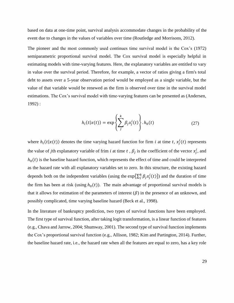
– see, for example, Figure 5, and this enhancement in performance is statistically significant as

demonstrated by a substantially large number of one-tailed t-tests of hypotheses involving all

combinations of 12 modelling frameworks, 9 categories of information, and 15 measures of 3

performance criteria, where the Null hypothesis 𝐻0 is: Average performance of modelling

33

framework 𝑋 fed with information category 𝑌 ≤ Average performance of modelling framework

𝑋′ fed with information category 𝑌′ – see Table 3 for an illustrative example of the typical outcome

of these hypothesis tests. In addition, market information (e.g., (log) stock prices, (log) excess

returns, volatility of stock returns / unsystematic risk, firm size as proxied by log (number of

outstanding shares × year end share price / total market value), its market value, or market value

of assets to total liabilities) on its own informs models better than accounting information on its

own. However, market and macroeconomic information combined slightly enhance the

performance of distress prediction models whether static or dynamic. Furthermore, empirical

results suggest that the choice of how a specific piece of information is modelled affects its

relevance in adding value to a prediction model. In fact, for example, with respect to the market

information category, log(price) is a better modelling choice compared to the price itself and

excess return is generally better than log(price).

34

Table 3: The p-value of t-tests to compare the average performance of models using ROC as measure of discriminatory power

This table presents the p-value of t-tests to compare the performance of models using ROC. The Null hypothesis (𝐻0) is: Average performance of modelling framework 𝑋 fed with

information category 𝑌 ≤ Average performance of modelling framework 𝑋′ fed with information category 𝑌′.

Models

DD

WT

DB

_1/ln

(age)_

FA

DD

WF

SB

_F

AL

1M

I

DD

WF

SB

_F

AM

I

DD

WF

SB

_F

AM

V

DD

WF

SB

_F

AM

VL

1M

I

DD

WF

SB

_F

AM

VM

I

DD

WF

SB

_M

V

DD

WF

SB

_M

VL

1M

I

DD

WF

SB

_M

VM

I

DD

WT

DB

_1/ln

(age)_

FA

DD

WT

DB

_1/ln

(age)_

FA

L1M

I

DD

WT

DB

_1/ln

(age)_

FA

MI

DD

WT

DB

_1/ln

(age)_

FA

MV

DD

WT

DB

_1/ln

(age)_

FA

MV

L1M

I

DD

WT

DB

_1/ln

(age)_

FA

MV

MI

DD

WT

DB

_1/ln

(age)_

MV

DD

WT

DB

_1/ln

(age)_

MV

L1M

I

DD

WT

DB

_1/ln

(age)_

MV

MI

DDWFSB_FA 0.007 0.973 0.000 0.000 0.000 0.000 0.000 0.000 0.000 0.000 0.000 0.000 0.000 0.000 0.000 0.000 0.000

DDWFSB_FAL1MI 1.000 0.000 0.000 0.000 0.000 0.000 0.000 0.000 0.000 0.000 0.000 0.000 0.000 0.000 0.000 0.000

DDWFSB_FAMI 0.000 0.000 0.000 0.000 0.000 0.000 0.000 0.000 0.000 0.000 0.000 0.000 0.000 0.000 0.000

DDWFSB_FAMV 0.145 0.000 0.000 0.000 0.000 0.000 0.000 0.915 0.885 0.000 0.000 0.000 0.000 0.000

DDWFSB_FAMVL1MI 0.000 0.000 0.000 0.000 0.000 0.000 0.942 0.929 0.000 0.000 0.000 0.000 0.000

DDWFSB_FAMVMI 0.001 0.000 0.711 0.004 0.002 1.000 1.000 0.667 0.009 0.006 0.627 0.001

DDWFSB_MV 0.034 0.999 0.978 0.690 1.000 1.000 0.997 0.845 0.663 0.999 0.386

DDWFSB_MVL1MI 0.999 0.997 0.978 1.000 1.000 0.999 0.946 0.857 1.000 0.780

DDWFSB_MVMI 0.001 0.001 1.000 1.000 0.465 0.007 0.005 0.344 0.001

DDWTDB_1/ln(age)_FA 0.036 1.000 1.000 0.995 0.534 0.323 0.998 0.032

DDWTDB_1/ln(age)_FAL1MI 1.000 1.000 0.997 0.795 0.583 0.999 0.233

DDWTDB_1/ln(age)_FAMI 0.359 0.000 0.000 0.000 0.000 0.000

DDWTDB_1/ln(age)_FAMV 0.000 0.000 0.000 0.000 0.000

DDWTDB_1/ln(age)_FAMVL1MI 0.002 0.002 0.422 0.001

DDWTDB_1/ln(age)_FAMVMI 0.071 0.994 0.066

DDWTDB_1/ln(age)_MV 0.996 0.233

DDWTDB_1/ln(age)_MVL1MI 0.000

DDWTDB_1/ln(age)_MVMI

35

Figure 5: Measures of Discriminatory Power (ROC, H, Gini, KS, IV) for New Models designed in

Different Static and Dynamic Frameworks and Fed with 3-Year Information

In regards to the second question, which considers the out-of-sample performance of dynamic

distress prediction models compare to the out-of-sample performance of static ones with respect

to sample type and sample period length, empirical evidence suggests that the out-of-sample

implementation of static models within a rolling horizon framework overcomes the a priori

limitation of their static nature. In fact, under several combinations of categories of information

(e.g., FAMV, FAMVMI, MV), the performance of static models is comparable to the performance

of the dynamic ones across all measures of all criteria. This finding suggests that static models are

not to be discarded and explains why static models are popular amongst practitioners – see, for

example, Figure 7. In addition, the performance of static models is consistent across different

combinations of information categories for all measures of all criteria except for information value

(IV) and Type I error – see, for example, Figure 5 and Figure 9.

36

Figure 6: Measures of Discriminatory Power (ROC, H, Gini, KS, IV) of New Static Models

Designed in Different Frameworks

Considering static models and with respect to T1 error, as a measure of correctness of categorical

prediction criterion, MDA seems to deliver a higher performance whereas PA is the worst

performer. Also, PA performance suggests that this modelling framework is good at properly

classifying healthy firms (i.e., it has the smallest Type II error), but relatively speaking, it poorly

classifies the distressed ones (i.e., it has the largest Type I error) – see, for example, Figure 9.

Figure 7: ROC of New Models Designed in Different Static and Dynamic Frameworks

Fed with 3-year Information

37

With respect to ROC, H, Gini and KS, as measures of discriminatory power, LA and PA

outperform other static models. However, considering IV as measure of discriminatory power,

LPA seems to deliver a higher performance whereas MDA is the worst performer – see, for

example, Figure 6. However, when static modelling frameworks are fed with both financial

accounting and macroeconomic information, there is a clear difference in discriminatory power

which suggests that macroeconomic information enhances the performance of LA and PA for

discriminatory power measures.

Figure 8: Measures of Correctness of Categorical Prediction of New Static Models Designed

in Different Frameworks

With respect to Pseudo-R2 and Log Likelihood, as measures of information content, LA and PA

outperform other static models when fed with accounting and macroeconomic information – see,

for example, Figure 10; however, LPA stands out as the best model when market information is

used. On the other hand, with respect to measures of quality of fit, such as Brier score, LA

outperforms other static models when fed with accounting and macroeconomic information - see,

for example,

Much like static models, empirical results suggest that dynamic models perform better when fed

with information beyond accounting one; in fact, the performance of dynamic models across most

measures of the three criteria under consideration is not only further enhanced when market

information is taken on board – see, for example, Figure 5, but it is consistent across all

38

combinations of categories of information that include market variables – see, for example, Figure

5.

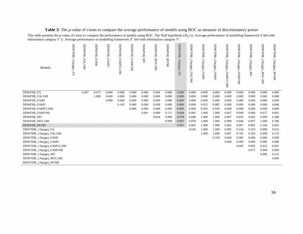
With respect to OCC, T2 and MR, as measures of correctness of categorical prediction,

DDWTDB_1/ln(age) and DDWTDB_ln(age) [baseline is ignored or equal to 1, and 1/ln(age) and

ln(age) are explanatory variables] are the best and second best performers, followed by DIWTIB-

1/ln(age) and DIWTIB-ln(age) (1/ln(age) and ln(age) are baselines or intercepts) as average

performers, and DDWFSB and DDWTDB-LPE being the worst ones – see, for example, Figure

9. Note however that, with respect to T1, DDWTDB-LPE is the best performer or amongst the

best performers regardless of the information categories taken into account. On the other hand,

DDWFSB and DDWTDB-VEX are, as expected, being the worst for any combination of

information categories that includes market information; however, when market information is not

considered, DDWFSB’s performance improves while DDWTDB-VEX’s performance remains

weak – see Figure 9.

With respect to ROC, H, Gini and KS, as measures of discriminatory power, DDWTDB_1/ln(age)

is the best performer amongst dynamic models, whereas DDWTDB-ln(age) and DDWFSB are the

worst performers – see Figure 5. Once again dynamic models perform better when fed with

information beyond accounting ones.

As to information content as measured by Pseudo-R2 and Log likelihood, DIWTIB_ln(age) (resp.

DDWFSB) outperform (underperform) other dynamic models – see, for example, Figure 10.

With respect to the quality of fit, under its BS measure, the performance of DIWTIB_1/ln(age)

(resp. DIWTIB_ln(age)) models fed with market variables outperform (resp. underperform) other

dynamic models - see, for example, To conclude our comparative analysis of static and dynamic

models, we would like to stress out that, in general, static modelling frameworks are as good

performers as dynamic ones when implemented under a dynamic scheme. This conclusion

suggests that the design of dynamic models along with the information they are fed with need more

attention from the academic community for this category of models to perform to the standard it

is expected from dynamic frameworks, on one hand, and to become a real contender for

practitioners, on one hand.

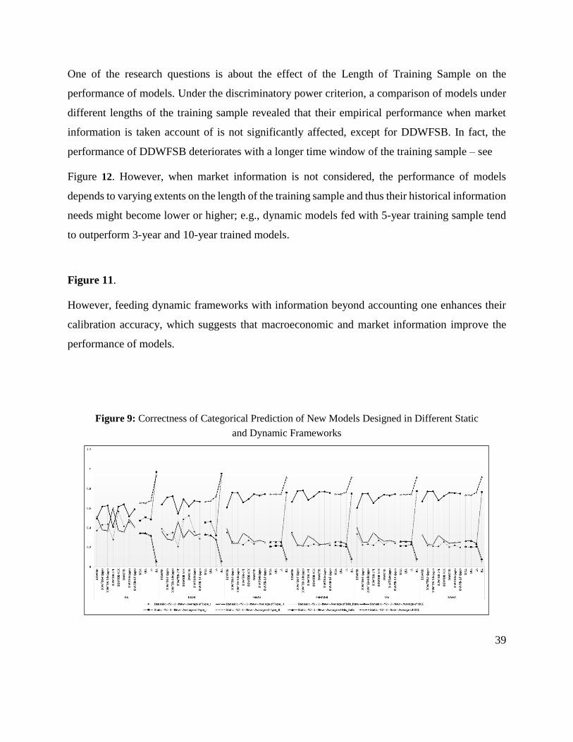
39

One of the research questions is about the effect of the Length of Training Sample on the

performance of models. Under the discriminatory power criterion, a comparison of models under

different lengths of the training sample revealed that their empirical performance when market

information is taken account of is not significantly affected, except for DDWFSB. In fact, the

performance of DDWFSB deteriorates with a longer time window of the training sample – see

Figure 12. However, when market information is not considered, the performance of models

depends to varying extents on the length of the training sample and thus their historical information

needs might become lower or higher; e.g., dynamic models fed with 5-year training sample tend

to outperform 3-year and 10-year trained models.

Figure 11.

However, feeding dynamic frameworks with information beyond accounting one enhances their

calibration accuracy, which suggests that macroeconomic and market information improve the

performance of models.

Figure 9: Correctness of Categorical Prediction of New Models Designed in Different Static

and Dynamic Frameworks

40

With respect to both static and dynamic models, under the correctness of categorical prediction

criterion, the performance profiles of both static and dynamic models are consistent across

different combinations of information categories, however they deliver different performances on

different performance measures with the exception of T2 and MR for which both static and

dynamic models deliver the same average performance figures – see Figure 9. This latter empirical

finding is explained by the fact that MR is a weighted combination of T1 and T2 errors and healthy

firms count for the majority of firms in our sample. However, although T1 and OCC are consistent

in the way they drive performance, they deliver different figures as expected. One notable

behaviour in performance is that of PA being the best performer amongst all static and dynamic

models with respect to T2 error, MR and OCC; whereas PA’s performance is consistently the

worst under T1 errors, on one hand, and the continuous-time hazard model with time-varying

baseline based on historical survival period (DDWFSB) is the worst performer across all measures,

on the other hand.

Under the discriminatory power criterion, the performance profile of both static and dynamic

models are also consistent across different combinations of information categories – see Figure 5.

Furthermore, their performance is similar for all measures of discriminatory power except for

information value (IV). Generally, DDWTDB_1/ln(age) and LA models are the best performers

once the models are fed with market information.

Figure 10: Log likelihood and Pseudo-R2 of New Dynamic and Static Models Fed

with Different Type of Information

41

As to the calibration accuracy criterion, under measures of both information content and quality

of fir, the dynamic model DIWTIB_ln(age) fed with FAMVMI has the highest Pseudo-R2, the

lowest Log Likelihood, and the lowest Brier score; therefore, it outperforms all other models

whether static or dynamic – see for Figure 10 and Error! Not a valid bookmark self-reference.

for example; however, market information boosts LPA models performance to become the best

amongst static models.

To conclude our comparative analysis of static and dynamic models, we would like to stress out

that, in general, static modelling frameworks are as good performers as dynamic ones when

implemented under a dynamic scheme. This conclusion suggests that the design of dynamic

models along with the information they are fed with need more attention from the academic

community for this category of models to perform to the standard it is expected from dynamic

frameworks, on one hand, and to become a real contender for practitioners, on one hand.

One of the research questions is about the effect of the Length of Training Sample on the

performance of models. Under the discriminatory power criterion, a comparison of models under

different lengths of the training sample revealed that their empirical performance when market

information is taken account of is not significantly affected, except for DDWFSB. In fact, the

performance of DDWFSB deteriorates with a longer time window of the training sample – see

42

Figure 12. However, when market information is not considered, the performance of models

depends to varying extents on the length of the training sample and thus their historical information

needs might become lower or higher; e.g., dynamic models fed with 5-year training sample tend

to outperform 3-year and 10-year trained models.

Figure 11: Brier Score of new dynamic and static models fed with different type of information

Figure 12: ROC of New Models Fed with Different Length and Type of Information

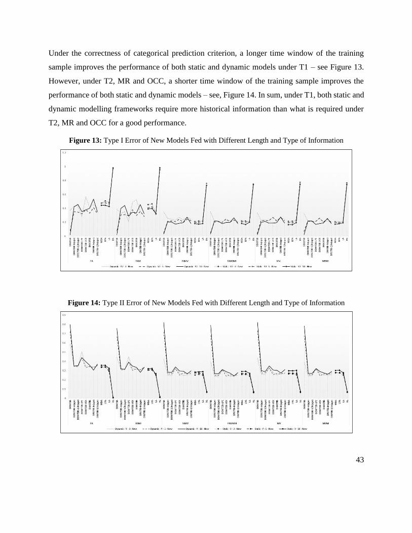
43

Under the correctness of categorical prediction criterion, a longer time window of the training

sample improves the performance of both static and dynamic models under T1 – see Figure 13.

However, under T2, MR and OCC, a shorter time window of the training sample improves the

performance of both static and dynamic models – see, Figure 14. In sum, under T1, both static and

dynamic modelling frameworks require more historical information than what is required under

T2, MR and OCC for a good performance.

Figure 13: Type I Error of New Models Fed with Different Length and Type of Information

Figure 14: Type II Error of New Models Fed with Different Length and Type of Information

44

Under the information content criterion and its measures; namely, Pseudo-R2 and Log likelihood,

most models fed with 5-year training sample outperform other models when market information

is ignored. However, when market variables are taken into account, a shorter time window of the

training sample improves the performance of both static and dynamic models – see, for example,

Figure 15.

Figure 15: Pseudo-R2 of New Models Fed with Different Length and Type of Information

Under Brier score, as a calibration accuracy measure, models fed with 5-year training sample

perform better when market information is ignored. However, when static and dynamic models

are fed with market information, a shorter time window of the training sample improves their

performance – see As suggested by one-dimensional ranking of distress prediction models, taking

into account different performance criteria and measures, there are considerable conflicts and ties

in ranking of models. Therefore, taking into account multiple criteria, one cannot make an

informed decision as to which model performs best. Although, we insist that one-dimensional

rankings are not to be discarded, we would like to propose a dynamic multi-criteria assessment,

which provides a single ranking under multiple criteria.

45

Figure 16. In sum, although accounting, market, and macroeconomic information are correlated

to varying degrees over time, market information proved to be the most informative prediction-

wise.

As suggested by one-dimensional ranking of distress prediction models, taking into account

different performance criteria and measures, there are considerable conflicts and ties in ranking of

models. Therefore, taking into account multiple criteria, one cannot make an informed decision as

to which model performs best. Although, we insist that one-dimensional rankings are not to be

discarded, we would like to propose a dynamic multi-criteria assessment, which provides a single

ranking under multiple criteria.

46

Figure 16: Brier Score of New Models Fed with Different Length and Type of Information

4.5.3. Multi criteria performance evaluation of distress prediction models

In this study we considered 12 forecasting frameworks (i.e., MDA, LPA, LA, PA, DDWFSB,

DDWTDB_ln(age), DDWTDB_1/ln(age), DDWTDB_LPE, DDWTDB_VEX, DDWOTIB,

DDWTIB_ln(age), and DDWTIB_1/ln(age)) which are fed with six groups of information (i.e.,

FA, FAMI, FAMV, FAMVMI, MV, and MVMI) using three different training periods (i.e., 3, 5

and 10-year information). Due to the superiority of models fed with FAMVMI in mono-criteria

rankings and also to save space, we only present the multi-criteria performance evaluation of

models fed with FAMVMI. Note however that the same findings are reached under other

combinations of information categories.

Setup 1 - Inputs: T1, BS and outputs: Pseudo-R2, ROC

In the first round of multi-criteria assessment using Malmquist DEA, we used T1 error (as a

measure of correctness of categorical prediction) and Brier score (as a measure of quality of fit) as

inputs, and Pseudo-R2 (as a measure of information content) and ROC (as a measure of

discriminatory power) as outputs.

47

Table 4, Table 5 and Table 6 provide the rankings of models based on the estimated efficiency

scores during period 2000 to 2014. For easier comparison, we provide a point which is calculated

based on the ranking of models over 15-year period.

With respect to the performance of models fed with 3-year training sample, DDWTDB-1/ln(age)

outperforms other models, following by DDWTDB-ln(age) and DIWTIB-ln(age) which are the

second and third best performers. Note that, although multi-criteria ranking of models suggest that

dynamic models are superior to the static ones, LA performs better than the other static models

and some dynamic ones.

Considering models fed with either 5 or 10-year training samples, DDWTDB-1/ln(age), DDWFSB

and DDWTDB-ln(age) are the best performers. Furthermore, the static model LA outperforms the

remaining static models. As the results of mono-criterion ranking suggest increasing the length of

the training sample improves the performance of DDWFSB under T1 error. In consistent to mono-

criterion, the results of multi-criteria ranking suggest that increasing the period of training sample

improves the performance of DDWFSB.

Comparing all models fed with 3, 5 and 10-year training sample, dynamic models perform much

better than static models. DDWFSB fed with 5-year information has the best performance over

15-year period, following by other duration dependent models which use ln(age) or 1/ln(age) as

baseline rate_ see Table 10 .

Setup 2 - Inputs: T2, BS and outputs: Pseudo-R2, ROC

In the second round of multi-criteria assessment using Malmquist, we used Type II error (as

measure of correctness of categorical prediction) and Brier score (as measure of quality of fit) as

inputs, and R2 (as measure of information content) and ROC (as measure of discriminatory power)

as outputs.

Table 7, Table 8 and Table 9 represent the ranking of models in each year based on the estimated

efficiency scores using Malmquist DEA. Conversely to the last round of multi-criteria assessment

where the static models underperform dynamic ones, the second round of assessment indicates that

48

PA outperforms other models. With respect to all length of training samples, the PA model

outperforms other models. However, the dynamic model of DDWTDB_1/ln(age) is ranked second

followed by DDWTDB_ln(age) with respect to all length of training samples.

With respect to all models fed with FAMVMI, the static model of PA fed with 5,3 and 10-year

information outperform other models over 15-year period. DDWTDB_1/ln(age) fed with 3,5-year

training sample is the second best performer, see Table 11.

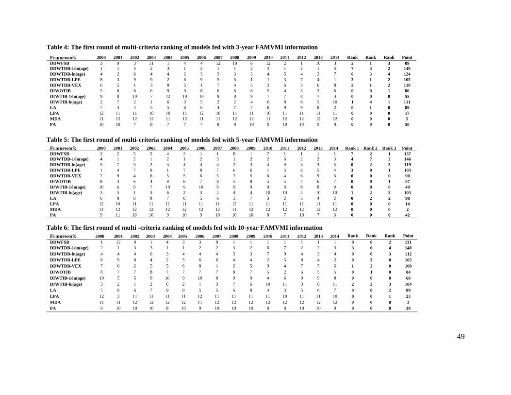
49

Table 4: The first round of multi-criteria ranking of models fed with 3-year FAMVMI information

Table 5: The first round of multi-criteria ranking of models fed with 5-year FAMVMI information

Framework 2000 2001 2002 2003 2004 2005 2006 2007 2008 2009 2010 2011 2012 2013 2014 Rank 1 Rank 2 Rank 3 Point

DDWFSB 2 2 5 5 4 3 1 1 8 1 7 1 1 1 1 7 2 1 137

DDWTDB-1/ln(age) 4 1 2 1 2 1 2 3 1 2 2 6 2 2 3 4 7 2 146

DDWTDB-ln(age) 5 7 3 2 3 4 4 4 2 3 4 9 3 3 5 0 2 5 119

DDWTDB-LPE 1 4 7 9 1 7 8 7 6 6 1 3 8 5 4 3 0 1 103

DDWTDB-VEX 7 9 4 6 5 5 6 5 7 5 6 4 6 9 6 0 0 0 90

DIWOTIB 8 3 6 4 8 6 7 8 5 8 5 5 7 6 7 0 0 1 87

DIWTIB-1/ln(age) 10 6 9 7 10 9 10 9 9 9 9 8 9 8 9 0 0 0 49

DIWTIB-ln(age) 3 5 1 3 6 2 3 2 4 4 10 10 4 10 10 1 2 3 103

LA 6 8 8 8 7 8 5 6 3 7 3 2 5 4 2 0 2 2 98

LPA 12 10 11 11 11 11 11 11 12 11 11 11 11 11 11 0 0 0 14

MDA 11 12 12 12 12 12 12 12 11 12 12 12 12 12 12 0 0 0 2

PA 9 11 10 10 9 10 9 10 10 10 8 7 10 7 8 0 0 0 42

Table 6: The first round of multi -criteria ranking of models fed with 10-year FAMVMI information

Framework 2000 2001 2002 2003 2004 2005 2006 2007 2008 2009 2010 2011 2012 2013 2014 Rank

1

Rank

2

Rank

3

Point

DDWFSB 1 12 9 1 4 3 3 9 1 1 1 1 1 1 1 9 0 2 131

DDWTDB-1/ln(age) 2 1 3 3 1 1 2 2 3 2 6 7 2 2 3 3 6 4 140

DDWTDB-ln(age) 4 4 4 6 3 4 4 4 5 3 7 9 4 3 4 0 0 3 112

DDWTDB-LPE 6 9 8 4 2 5 6 6 4 4 2 5 8 4 2 0 3 0 105

DDWTDB-VEX 7 6 2 5 5 6 8 1 2 5 9 4 7 7 6 1 2 0 100

DIWOTIB 8 7 7 8 7 7 7 7 8 7 5 2 6 5 5 0 1 0 84

DIWTIB-1/ln(age) 10 5 5 9 10 9 10 8 9 9 4 6 9 9 8 0 0 0 60

DIWTIB-ln(age) 3 2 1 2 6 2 1 3 7 6 10 11 3 8 11 2 3 3 104

LA 5 8 6 7 9 8 5 5 6 8 3 3 5 6 7 0 0 2 89

LPA 12 3 11 11 11 11 12 11 11 11 11 10 11 11 10 0 0 1 23

MDA 11 11 12 12 12 12 11 12 12 12 12 12 12 12 12 0 0 0 3

PA 9 10 10 10 8 10 9 10 10 10 8 8 10 10 9 0 0 0 39

Framework 2000 2001 2002 2003 2004 2005 2006 2007 2008 2009 2010 2011 2012 2013 2014 Rank

1

Rank

2

Rank

3

Point

DDWFSB 3 9 3 11 1 4 4 12 10 6 12 2 1 10 3 2 1 3 89

DDWTDB-1/ln(age) 1 1 5 2 3 1 2 1 1 2 3 1 2 1 5 7 4 2 149

DDWTDB-ln(age) 4 2 6 4 4 2 3 3 3 3 4 5 4 2 7 0 3 4 124

DDWTDB-LPE 8 3 9 9 2 8 9 5 5 1 1 3 7 4 1 3 1 2 105

DDWTDB-VEX 6 5 1 3 8 5 1 7 4 5 2 6 3 6 8 2 1 2 110

DIWOTIB 5 6 8 6 9 9 8 6 6 8 5 4 5 3 6 0 0 1 86

DIWTIB-1/ln(age) 9 8 10 7 12 10 10 9 8 9 7 7 8 7 4 0 0 0 55

DIWTIB-ln(age) 2 7 2 1 6 3 5 2 2 4 6 8 6 5 10 1 4 1 111

LA 7 4 4 5 5 6 6 4 7 7 8 9 9 8 2 0 1 0 89

LPA 12 11 11 10 10 11 12 10 11 11 10 11 11 11 11 0 0 0 17

MDA 11 12 12 12 11 12 11 11 12 12 11 12 12 12 12 0 0 0 5

PA 10 10 7 8 7 7 7 8 9 10 9 10 10 9 9 0 0 0 50

50

Table 7: The second round of multi-criteria ranking of models fed with 3-year FAMVMI information

Framework 2000 2001 2002 2003 2004 2005 2006 2007 2008 2009 2010 2011 2012 2013 2014 Rank 1 Rank 2 Rank 3 Point

DDWFSB 3 10 8 3 1 5 5 1 10 10 2 8 10 11 10 2 1 2 83

DDWTDB-1/ln(age) 4 3 3 5 4 1 1 3 2 2 3 3 3 3 3 2 2 8 137

DDWTDB-ln(age) 6 7 5 4 5 3 2 4 3 3 5 6 5 5 5 0 1 3 112

DDWTDB-LPE 7 9 6 1 11 9 8 8 7 9 10 5 4 8 8 1 0 0 70

DDWTDB-VEX 5 5 9 6 10 8 6 7 8 6 9 2 2 2 2 0 4 0 93

DIWOTIB 8 6 7 8 9 7 9 9 6 5 4 4 7 7 6 0 0 0 78

DIWTIB-1/ln(age) 10 8 10 10 12 10 10 10 9 7 6 7 9 6 7 0 0 0 49

DIWTIB-ln(age) 2 2 2 7 6 4 4 5 4 4 7 9 6 9 9 0 3 0 100

LA 9 4 4 9 3 6 7 6 5 8 8 10 8 4 4 0 0 1 85

PA 1 1 1 2 2 2 3 2 1 1 1 1 1 1 1 10 4 1 159

LPA 12 11 11 11 8 11 12 11 11 11 11 11 11 10 11 0 0 0 17

MDA 11 12 12 12 7 12 11 12 12 12 12 12 12 12 12 0 0 0 7

Table 8: The second round of multi-criteria ranking of models fed with 5-year FAMVMI information

Framework 2000 2001 2002 2003 2004 2005 2006 2007 2008 2009 2010 2011 2012 2013 2014 Rank 1 Rank 2 Rank 3 Point

DDWFSB 10 10 10 12 12 12 2 12 12 10 12 10 9 11 10 0 1 0 26

DDWTDB-1/ln(age) 3 3 3 3 2 2 4 2 2 2 3 6 3 3 2 0 6 7 137

DDWTDB-ln(age) 4 4 4 6 3 3 5 4 3 3 6 8 4 4 7 0 0 4 112

DDWTDB-LPE 9 8 6 2 11 5 6 6 5 8 10 3 5 5 6 0 1 1 85

DDWTDB-VEX 6 6 9 4 6 7 8 8 6 7 4 2 2 2 4 0 3 0 99

DIWOTIB 7 7 7 9 7 8 9 7 8 6 5 5 7 6 5 0 0 0 77

DIWTIB-1/ln(age) 8 9 8 8 10 9 10 9 9 9 7 7 10 8 8 0 0 0 51

DIWTIB-ln(age) 2 2 2 5 5 4 3 3 4 4 8 9 8 10 11 0 3 2 100

LA 5 5 5 7 4 6 7 5 7 5 2 4 6 7 3 0 1 1 102

PA 1 1 1 1 1 1 1 1 1 1 1 1 1 1 1 15 0 0 165

LPA 12 11 11 10 8 11 11 10 10 11 9 11 11 9 9 0 0 0 26

MDA 11 12 12 11 9 10 12 11 11 12 11 12 12 12 12 0 0 0 10

Table 9: The second round of multi-criteria ranking of models fed with 10-year FAMVMI information

Framework 2000 2001 2002 2003 2004 2005 2006 2007 2008 2009 2010 2011 2012 2013 2014 Rank 1 Rank 2 Rank 3 Point

DDWFSB 11 12 12 12 12 11 9 12 12 12 12 12 12 12 12 0 0 0 5

DDWTDB-1/ln(age) 2 2 3 2 2 3 3 2 2 2 2 6 2 2 2 0 11 3 143

DDWTDB-ln(age) 4 5 4 4 3 4 4 4 4 3 4 8 3 4 4 0 0 3 118

DDWTDB-LPE 8 8 5 9 11 5 6 7 7 8 7 3 4 6 7 0 0 1 79

DDWTDB-VEX 6 7 8 5 5 7 7 8 8 7 9 2 6 3 3 0 1 2 89

DIWOTIB 7 9 6 7 6 6 8 6 6 6 3 4 8 7 5 0 0 1 86

DIWTIB-1/ln(age) 9 10 7 8 8 9 10 9 9 9 6 7 9 9 8 0 0 0 53

DIWTIB-ln(age) 3 3 2 3 4 2 2 3 3 4 8 9 5 8 9 0 3 5 112

LA 5 6 9 6 7 8 5 5 5 5 5 5 7 5 6 0 0 0 91

PA 1 1 1 1 1 1 1 1 1 1 1 1 1 1 1 15 0 0 165

LPA 12 4 10 10 9 10 12 10 10 10 10 10 10 10 10 0 0 0 33

MDA 10 11 11 11 10 12 11 11 11 11 11 11 11 11 11 0 0 0 16

51

5. Conclusion

Prediction of corporate distress is crucial for many decision makers in finance and investment. Although

a large number of models have been designed to predict bankruptcy and distress, the relative performance

evaluation of competing distress models remains an exercise that is one-dimensional in nature, which

results in conflicting rankings of models from one performance criterion to another. In this study, we

proposed an orientation-free super-efficiency Malmquist DEA, which provides a single ranking, based

on multiple performance criteria. In addition, we exercised a comprehensive comparative analysis of the

most famous static and dynamic distress prediction models. For this, we used several measures under

four commonly employed criteria (i.e., the discriminatory power, the information content, the calibration

accuracy, and the correctness of categorical prediction) in the literature. Furthermore, we addressed the

following important questions: What category of information or combination of categories of information

enhances the predictive ability of models best? and How the out-of-sample performance of dynamic

distress prediction models compare to the out-of-sample performance of static ones with respect to

sample type and sample period length?

Our main findings could be classified as follows. Firstly, the proposed multi-criteria dynamic framework

provides a useful tool in evaluating the relative performance of distress prediction models over time.

Secondly, conversely to the one-dimensional ranking, the multidimensional ranking of models provides

more consistent results. However, in case of a significant inconsistency between rankings of a model

using Type I and Type II errors (i.e. PA model), multi-criteria rankings of a model using each of these

two measures would also present inconsistency. Third, empirical results suggest that dynamic models,

specifically DDWTDB_1/ln(age) and DDEWTDB_ln(age) are always amongst the best distress

prediction models and show consistency in multi-criteria ranking using different combinations of

measures. Forth, models fed with shorter training sample period (i.e. 3-year training period) length are

superior in performance. Fifth, most modelling frameworks show improvement in performance by taking

account of features beyond accounting-based information (i.e. FAMVMI and FAMV).

52

Table 10: The first round of multi-criteria ranking of models fed with FAMVMI information

Framework 2000 2001 2002 2003 2004 2005 2006 2007 2008 2009 2010 2011 2012 2013 2014 Total

rank

DDWFSB_05 5 1 14 14 13 9 4 1 17 1 19 1 2 12 1 1

DDWTDB_1/ln(age)_03 1 15 25 17 14 1 2 3 7 4 11 3 4 2 7 2

DDWFSB_10 9 36 13 1 7 8 14 24 1 2 2 2 1 1 2 3

DDWTDB_1/ln(age)_05 7 1 6 9 8 1 12 7 2 7 10 20 11 20 13 4

DDWTDB_1/ln(age)_10 15 1 4 3 1 5 13 6 13 8 9 14 12 10 23 5

DDWTDB_ln(age)_03 8 17 26 21 18 4 3 9 10 5 15 11 6 3 9 6

DDWTDB_ln(age)_10 16 10 5 6 5 10 16 11 16 12 12 21 16 13 24 7

DDWTDB_ln(age)_05 10 12 7 10 11 11 19 8 3 9 14 27 14 23 15 7

DIWTIB_ln(age)_03 1 25 21 16 25 6 6 4 8 6 20 25 8 6 19 9

DDWTDB_LPE_03 14 19 29 29 6 23 11 17 21 3 3 5 9 5 3 10

DDWTDB_VEX_03 12 23 20 18 28 13 1 22 15 11 4 13 5 7 10 11

DDWTDB_LPE_10 20 20 12 4 1 16 20 16 14 13 5 9 26 15 22 12

DIWTIB_ln(age)_05 6 8 3 12 20 1 17 5 5 10 26 31 18 31 26 13

DIWTIB_ln(age)_10 16 1 1 2 10 7 9 10 20 17 28 29 15 21 34 14

DDWTDB_VEX_10 21 13 2 5 9 18 23 2 12 15 25 8 24 19 27 15

DDWTDB_LPE_05 1 7 16 24 4 17 30 18 9 16 1 16 25 26 14 16

LA_10 19 18 10 7 16 25 18 15 19 19 6 7 19 17 28 17

DIWOTIB_10 22 16 11 8 12 20 21 21 22 18 8 6 21 16 25 18

DDWFSB_03 1 27 22 34 1 12 5 36 33 20 36 4 3 14 5 19

LA_05 23 14 17 20 21 21 22 14 4 21 13 15 20 24 12 20

DIWOTIB_03 11 24 28 26 29 24 10 19 24 23 17 10 7 4 8 21

DDWTDB_VEX_05 27 21 8 15 17 14 28 12 11 14 18 17 22 30 16 22

LA_03 13 22 24 23 23 19 7 13 26 22 27 28 13 9 4 23

DIWOTIB_05 28 6 15 13 22 15 29 20 6 24 16 18 23 27 17 24

DIWTIB_1/ln(age)_10 26 11 9 11 19 28 27 23 23 25 7 12 27 22 29 25

DIWTIB_1/ln(age)_03 18 26 30 27 36 30 15 28 29 27 21 23 10 8 6 26

PA_03 24 31 27 28 26 22 8 25 31 32 31 30 17 11 11 27

DIWTIB_1/ln(age)_05 30 9 19 19 30 26 32 27 18 26 24 26 29 29 20 28

PA_10 25 30 18 22 15 29 24 26 27 28 22 19 28 25 30 29

PA_05 29 29 23 25 24 27 31 29 25 31 23 22 30 28 18 30

LPA_10 36 5 31 30 27 34 35 30 32 29 30 24 35 32 33 31

LPA_03 33 32 33 33 34 31 26 34 35 35 34 35 31 18 21 32

LPA_05 34 28 35 32 31 33 33 32 30 33 29 33 32 34 32 33

MDA_10 35 34 32 31 32 35 34 31 34 30 32 32 36 35 35 34

MDA_03 32 33 34 35 35 32 25 35 36 36 35 36 33 33 31 35

MDA_05 31 35 36 36 33 36 36 33 28 34 33 34 34 36 36 36

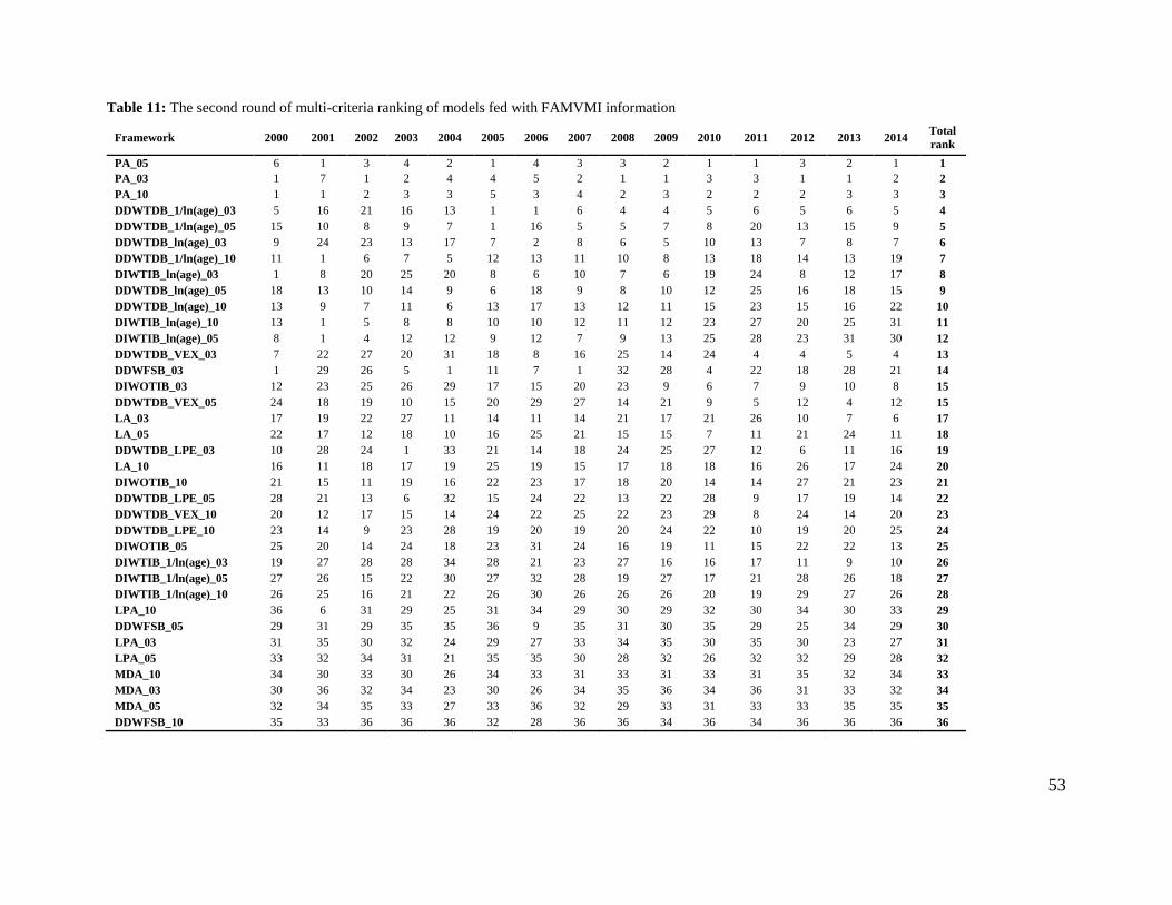
53

Table 11: The second round of multi-criteria ranking of models fed with FAMVMI information

Framework 2000 2001 2002 2003 2004 2005 2006 2007 2008 2009 2010 2011 2012 2013 2014 Total

rank

PA_05 6 1 3 4 2 1 4 3 3 2 1 1 3 2 1 1

PA_03 1 7 1 2 4 4 5 2 1 1 3 3 1 1 2 2

PA_10 1 1 2 3 3 5 3 4 2 3 2 2 2 3 3 3

DDWTDB_1/ln(age)_03 5 16 21 16 13 1 1 6 4 4 5 6 5 6 5 4

DDWTDB_1/ln(age)_05 15 10 8 9 7 1 16 5 5 7 8 20 13 15 9 5

DDWTDB_ln(age)_03 9 24 23 13 17 7 2 8 6 5 10 13 7 8 7 6

DDWTDB_1/ln(age)_10 11 1 6 7 5 12 13 11 10 8 13 18 14 13 19 7

DIWTIB_ln(age)_03 1 8 20 25 20 8 6 10 7 6 19 24 8 12 17 8

DDWTDB_ln(age)_05 18 13 10 14 9 6 18 9 8 10 12 25 16 18 15 9

DDWTDB_ln(age)_10 13 9 7 11 6 13 17 13 12 11 15 23 15 16 22 10

DIWTIB_ln(age)_10 13 1 5 8 8 10 10 12 11 12 23 27 20 25 31 11

DIWTIB_ln(age)_05 8 1 4 12 12 9 12 7 9 13 25 28 23 31 30 12

DDWTDB_VEX_03 7 22 27 20 31 18 8 16 25 14 24 4 4 5 4 13

DDWFSB_03 1 29 26 5 1 11 7 1 32 28 4 22 18 28 21 14

DIWOTIB_03 12 23 25 26 29 17 15 20 23 9 6 7 9 10 8 15

DDWTDB_VEX_05 24 18 19 10 15 20 29 27 14 21 9 5 12 4 12 15

LA_03 17 19 22 27 11 14 11 14 21 17 21 26 10 7 6 17

LA_05 22 17 12 18 10 16 25 21 15 15 7 11 21 24 11 18

DDWTDB_LPE_03 10 28 24 1 33 21 14 18 24 25 27 12 6 11 16 19

LA_10 16 11 18 17 19 25 19 15 17 18 18 16 26 17 24 20

DIWOTIB_10 21 15 11 19 16 22 23 17 18 20 14 14 27 21 23 21

DDWTDB_LPE_05 28 21 13 6 32 15 24 22 13 22 28 9 17 19 14 22

DDWTDB_VEX_10 20 12 17 15 14 24 22 25 22 23 29 8 24 14 20 23

DDWTDB_LPE_10 23 14 9 23 28 19 20 19 20 24 22 10 19 20 25 24

DIWOTIB_05 25 20 14 24 18 23 31 24 16 19 11 15 22 22 13 25

DIWTIB_1/ln(age)_03 19 27 28 28 34 28 21 23 27 16 16 17 11 9 10 26

DIWTIB_1/ln(age)_05 27 26 15 22 30 27 32 28 19 27 17 21 28 26 18 27

DIWTIB_1/ln(age)_10 26 25 16 21 22 26 30 26 26 26 20 19 29 27 26 28

LPA_10 36 6 31 29 25 31 34 29 30 29 32 30 34 30 33 29

DDWFSB_05 29 31 29 35 35 36 9 35 31 30 35 29 25 34 29 30

LPA_03 31 35 30 32 24 29 27 33 34 35 30 35 30 23 27 31

LPA_05 33 32 34 31 21 35 35 30 28 32 26 32 32 29 28 32

MDA_10 34 30 33 30 26 34 33 31 33 31 33 31 35 32 34 33

MDA_03 30 36 32 34 23 30 26 34 35 36 34 36 31 33 32 34

MDA_05 32 34 35 33 27 33 36 32 29 33 31 33 33 35 35 35

DDWFSB_10 35 33 36 36 36 32 28 36 36 34 36 34 36 36 36 36

54

Appendix A: Comparison between different failure prediction frameworks

Author Models Criteria (Measure) Result

Panel I: Comparison between traditional statistical models

Press and Wilson (1976) LA and MDA models Correctness of categorical prediction

(T1 and T2 errors)

Two models unlikely will give significantly

different results.

Collins and Green

(1982)

LPM, MDA and LA models Correctness of categorical prediction

(OCC, T1 and T2)

The models produce identical, uniformly results.

Lo (1986) MDA and LA models Power of models There is not differences between models.

Theodossiou (1991)

LPM, LA, and PA models Correctness of categorical prediction

(T1 and T2 errors), Calibration (BS),

Information content (pseudo-R2)

logit model outperforms others; CONFLICT in

ranking of others with respect to different

measures

Lennox (1999) LA, PA, and MDA models Correctness of categorical prediction

(T1 and T2)

A well-specified non-linear PA and LA are

superior over DA

Bandyopadhyay (2006)

MDA models and logit models

Correctness of categorical prediction

(OCC, T1 and T2)

Discriminatory power (ROC),

Information content (pseudo-R2, LL)

CONFLICT in rankings using different criteria

and measures

Tinoco and Wilson

(2013)

logit models taking to

accounting different categories

of features

Discriminatory power (ROC, Gini,

KS), Calibration accuracy (HL)

CONFLICT in rankings using different criteria

and measures

Panel II: Comparison between traditional statistical models and survival analysis models

Luoma and Laitinen

(1991)

Cox-hazard, MDA and LA

models

Correctness of categorical prediction

(T1 and T2)

SA model is inferior than MDA and LA models

Shumway (2001) Discrete-time SA model, MDA,

LA and PA

Correctness of categorical prediction

(OCC)

SA model which, encompasses both accounting

and market information (respectively, only

accounting information) outperforms

(respectively, underperforms) other statistical

techniques

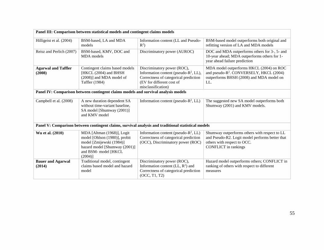
55

Panel III: Comparison between statistical models and contingent claims models

Hilligeist et al. (2004) BSM-based, LA and MDA

models

Information content (LL and Pseudo-

R2)

BSM-based model outperforms both original and

refitting version of LA and MDA models

Reisz and Perlich (2007) BSM-based, KMV, DOC and

MDA models

Discriminatory power (AUROC) DOC and MDA outperforms others for 3-, 5- and

10-year ahead; MDA outperforms others for 1-

year ahead failure prediction

Agarwal and Taffler

(2008)

Contingent claims based models

[HKCL (2004) and BHSH

(2008)] and MDA model of

Taffler (1984)

Discriminatory power (ROC),

Information content (pseudo-R2, LL),

Correctness of categorical prediction

(EV for different cost of

misclassification)

MDA model outperforms HKCL (2004) on ROC

and pseudo-R2. CONVERSELY, HKCL (2004)

outperforms BHSH (2008) and MDA model on

LL.

Panel IV: Comparison between contingent claims models and survival analysis models

Campbell et al. (2008) A new duration dependent SA

without time-variant baseline,

SA model [Shumway (2001)]

and KMV model

Information content (pseudo-R2, LL)

The suggested new SA model outperforms both

Shumway (2001) and KMV models.

Panel V: Comparison between contingent claims, survival analysis and traditional statistical models

Wu et al. (2010) MDA [Altman (1968)], Logit

model [Ohlson (1980)], probit

model [Zmijewski (1984)]

hazard model [Shumway (2001)]

and BSM- model [HKCL

(2004)]

Information content (pseudo-R2, LL)

Correctness of categorical prediction

(OCC), Discriminatory power (ROC)

Shumway outperforms others with respect to LL

and Pseudo-R2. Logit model performs better that

others with respect to OCC.

CONFLICT in rankings

Bauer and Agarwal

(2014)

Traditional model, contingent

claims based model and hazard

model

Discriminatory power (ROC),

Information content (LL, R2) and

Correctness of categorical prediction

(OCC, T1, T2)

Hazard model outperforms others; CONFLICT in

ranking of others with respect to different

measures

56

References

Abdou, H.A., Pointon, J. (2011). Credit scoring, statistical techniques and evaluation criteria: A

review of the literature. Intelligent Systems in Accounting, Finance and Management, 18 (2-

3), 59–88.

Agarwal, V., Taffler, R. (2008). Comparing the performance of market-based and accounting-based

bankruptcy prediction models. Journal of Banking & Finance, 32(8), 1541–1551.

Aktug, R.E. (2014). A Critique of the Contingent Claims Approach to Sovereign Risk Analysis.

Emerging Markets Finance and Trade, 50(1), 294–308.

Allison, P.D. (1982). Discrete-time methods for the analysis of event histories. Sociological

methodology, 13(1), 61–98.

Altman, E. (1983). Corporate financial distress: A complete guide to predicting. In John

Wiley and Sons (Ed.), Avoiding and dealing with bankruptcy.

Altman, E.I. (1982). Accounting implications of failure prediction models. Journal of Accounting,

Auditing and Finance, 2, 4–19.

Altman, E.I. (1968). Financial ratios, discriminant analysis and the prediction of corporate

bankruptcy. The journal of finance, 23(4), 589–609.

Altman, E.I., Haldeman, R.G., Narayanan, P. (1977). ZETA analysis A new model to identify

bankruptcy risk of corporations. Journal of banking & finance, 1(1), 29–54.

Andersen, P.K. (1992). Repeated assessment of risk factors in survival analysis. Statistical Methods

in Medical Research. 1(3), 297–315.

Anderson, R. (2007). The credit scoring toolkit, Theory and practice for retail credit risk

management and decision automation. New York: OXFORD university press,

Aziz, M.A., Dar, H.A. (2006). Predicting corporate bankruptcy: where we stand? Corporate

governance. 6(1), 18–33.

Balcaen, S., Ooghe, H. (2006). 35 years of studies on business failure: an overview of the classic

statistical methodologies and their related problems. The British Accounting Review, 38(1),

63–93.

Bandyopadhyay, A. (2006). Predicting probability of default of Indian corporate bonds: logistic and

Z-score model approaches. Journal of Risk Finance, 7 (3), 255–272.

Bauer, J., Agarwal, V. (2014). Are hazard models superior to traditional bankruptcy prediction

approaches? A comprehensive test. Journal of Banking & Finance, 40, 432–442.

Beaver, W.H., (1968). Alternative accounting measures as predictors of failure. Accounting review,

43(1),113–122.

Beaver, W.H. (1966). Financial Ratios as Predictors of Failure. Journal of Accounting Research, 4,

71-111.

Beck, N., Katz, J.N., Tucker, R. (1998). Taking time seriously: Time-series-cross-section analysis

with a binary dependent variable. American Journal of Political Science, 42(4), 1260–1288.

Bellotti, T., Crook, J. (2009). Forecasting and Stress Testing Credit Card Default using Dynamic

Models. International Journal of Forecasting, 29(4),563-574.

Bellovary, J.L., Giacomino, D.E., Akers, M.D. (2007). A review of bankruptcy prediction studies:

1930 to present. Journal of Financial Education, 33,1–42.

57

Bharath, S.T., Shumway, T. (2008). Forecasting default with the Merton distance to default model.

Review of Financial Studies,21(3), 1339–1369.

Black, F., Scholes, M., (1973). The pricing of options and corporate liabilities. The journal of

political economy 637–654.

Blum, M. (1974). Failing company discriminant analysis. Journal of Accounting Research, 12(1),

1–25.

Campbell, J.Y., Hilscher, J., Szilagyi, J. (2008). In search of distress risk. The Journal of Finance,

63(6), 2899–2939.

Caves, D.W., Christensen, L.R., Diewert, W.E., 1982. The Economic Theory of Index Numbers and

the Measurement of Input, Output, and Productivity. Econometrica 50, 1393–1414.

Charalambakis, E.C., Garrett, I., (2015). On the prediction of financial distress in developed and

emerging markets: Does the choice of accounting and market information matter? A

comparison of UK and Indian Firms. Rev Quant Finan Acc 47, 1–28.

Charitou, A., Neophytou, E., Charalambous, C., (2004). Predicting corporate failure: empirical

evidence for the UK. European Accounting Review 13, 465–497.

Charnes, A., Cooper, W.W., Rhodes, E., 1978. Measuring the efficiency of decision making units.

European journal of operational research 2, 429–444.

Chava, S., Jarrow, R.A. (2004). Bankruptcy prediction with industry effects. Review of Finance 8(4),

537–569.

Chen, L.-S., Yen, M.-F., Wu, H.-M., Liao, C.-S., Liou, D.-M., Kuo, H.-S., Chen, T.H.-H. (2005).

Predictive survival model with time-dependent prognostic factors: development of

computer-aided SAS Macro program. Journal of evaluation in clinical practice, 11(2), 181–

193.

Chen, M.-Y. (2011). Predicting corporate financial distress based on integration of decision tree

classification and logistic regression. Expert Systems with Applications, 38(9), 11261–11272.

Cleary, S., Hebb, G. (2016). An efficient and functional model for predicting bank distress: In and

out of sample evidence. Journal of Banking & Finance, 64, 101–111.

Collins, R.A., Green, R.D. (1982). Statistical methods for bankruptcy forecasting. Journal of

Economics and Business,34(4), 349–354.

Cooper, W.W., Seiford, L.M., Tone, K., 2006. Introduction to data envelopment analysis and its

uses: with DEA-solver software and references. Springer Science & Business Media.

Cox, D.R. (1972). Regression models and life-tables. Journal of Royal Statistical Society Series B:

Methodological,34(2), 187–220.

Crapp, H.R., Stevenson, M. (1987). Development of a method to assess the relevant variables and

the probability of financial distress. Australian journal of management,12(2), 221–236.

Deakin, E.B. (1972). A discriminant analysis of predictors of business failure. Journal of Accounting

Research,10(2),167–179.

du Jardin, P. (2015). Bankruptcy prediction using terminal failure processes. European Journal of

Operational Research, 242(1), 286–303.

du Jardin, P., Séverin, E. (2012). Forecasting financial failure using a Kohonen map: A comparative

study to improve model stability over time. European Journal of Operational Research,

221(2), 378–396.

58

Eisenbeis, R.A. (1977). Pitfalls in the Application of Discriminant Analysis in Business, Finance,

and Economics. The Journal of Finance, 32(3), 875-900.

Färe, R., Grosskopf, S., Lindgren, B., Roos, P., 1992. Productivity Changes in Swedish

Pharamacies 1980–1989: A Non-Parametric Malmquist Approach, in: Jr, T.R.G., Lovell,

C.A.K. (Eds.), International Applications of Productivity and Efficiency Analysis.

Springer Netherlands, pp. 81–97.

Färe, R., Grosskopf, S., Norris, M., Zhang, Z., 1994. Productivity Growth, Technical Progress,

and Efficiency Change in Industrialized Countries. The American Economic Review 84,

66–83.

Fedorova, E., Gilenko, E., Dovzhenko, S. (2013). Bankruptcy prediction for Russian companies:

Application of combined classifiers. Expert Systems with Applications, 40(18), 7285–7293.

Geng, R., Bose, I., Chen, X. (2015). Prediction of financial distress: An empirical study of listed

Chinese companies using data mining. European Journal of Operational Research, 241(1),

236–247.

Gilbert, L.R., Menon, K., Schwartz, K.B. (1990). Predicting Bankruptcy for Firms in Financial

Distress. Journal of Business Finance & Accounting, 17(1), 161–171.

Grice, J.S., Ingram, R.W., 2001. Tests of the generalizability of Altman’s bankruptcy prediction

model. Journal of Business Research 54, 53–61.

Hamer, M.M. (1983). Failure prediction: Sensitivity of classification accuracy to alternative

statistical methods and variable sets. Journal of Accounting and Public Policy, 2(4), 289–

307.

Hernandez Tinoco, M., Wilson, N. (2013). Financial distress and bankruptcy prediction among listed

companies using accounting, market and macroeconomic variables. International Review of

Financial Analysis, 30, 394–419.

Hillegeist, S.A., Keating, E.K., Cram, D.P., Lundstedt, K.G. (2004). Assessing the probability of

bankruptcy. Review of Accounting Studies, 9(1), 5–34.

Jackson, R.H., Wood, A. (2013). The performance of insolvency prediction and credit risk models

in the UK: A comparative study. The British Accounting Review, 45(3), 183–202.

Kim, M.H., Partington, G. (2014). Dynamic forecasts of financial distress of Australian firms.

Australian Journal of Management, 1-26.

Laitinen, E.K., Suvas, A. (2016). Financial distress prediction in an international context:

Moderating effects of Hofstede’s original cultural dimensions. Journal of Behavioural and

Experimental Finance, 9, 98–118.

Lane, W.R., Looney, S.W., Wansley, J.W. (1986). An application of the Cox proportional hazards

model to bank failure. Journal of Banking & Finance, 10 (4), 511–531.

LeClere, M.J. (2000). The occurrence and timing of events: Survival analysis applied to the study of

financial distress. Journal of Accounting Literature, 19, 158.

Lennox, C. (1999). Identifying failing companies: a re-evaluation of the logit, probit and DA

approaches. Journal of Economics and Business, 51(4), 347–364.

Lo, A.W. (1986). Logit versus discriminant analysis: A specification test and application to corporate

bankruptcies. Journal of Econometrics ,31(2), 151–178.

Luoma, M., Laitinen, E.K. (1991). Survival analysis as a tool for company failure prediction.

Omega,19(6), 673–678.

59

Lyandres, E., Zhdanov, A. (2013). Investment opportunities and bankruptcy prediction. Journal of

Financial Markets, 16(3), 439–476.

Malmquist, S., 1953. Index numbers and indifference surfaces. Trabajos de Estadistica 4, 209–

242.

Martin, D. (1977). Early warning of bank failure: A logit regression approach. Journal of Banking

& Finance, 1(3), 249–276.

McLeay, S. (1986). Student's t and the distribution of financial ratios. Journal of Business Finance

& Accounting, 13(2), 209-222.

Mensah, Y.M., 1984. An Examination of the Stationarity of Multivariate Bankruptcy Prediction

Models: A Methodological Study. Journal of Accounting Research 22, 380–395.

Merton, R.C., 1974. On the pricing of corporate debt: The risk structure of interest rates*. The

Journal of Finance 29, 449–470.

Meyer, P.A., Pifer, H.W. (1970). Prediction of bank failures. The Journal of Finance, 25(4), 853–

868.

Mousavi, M.M., Ouenniche, J., Xu, B. (2015). Performance evaluation of bankruptcy prediction

models: An orientation-free super-efficiency DEA-based framework. International Review

of Financial Analysis, 42, 64–75.

Neves, J.C., Vieira, A. (2006). Improving bankruptcy prediction with Hidden Layer Learning Vector

Quantization. European Accounting Review, 15(2), 253–271.

Ohlson, J.A. (1980). Financial ratios and the probabilistic prediction of bankruptcy. Journal of

accounting research, 18(1), 109–131.

Pacheco, J., Casado, S., Núñez, L. (2009). A variable selection method based on Tabu search for

logistic regression models. European Journal of Operational Research, 199(2), 506–511.

Pacheco, J., Casado, S., Nuñez, L. (2007). Use of VNS and TS in classification: variable selection

and determination of the linear discrimination function coefficients. IMA Journal of

Management Mathematics, 18(2), 191–206.

Pacheco, J., Casado, S., Nuñez, L., 2007. Use of VNS and TS in classification: variable selection

and determination of the linear discrimination function coefficients. IMA J Management

Math 18, 191–206.

Platt, H., Platt, M. (2012). Corporate board attributes and bankruptcy. Journal of Business Research,

65(8), 1139–1143.

Press, S.J., Wilson, S. (1978). Choosing between Logistic Regression and Discriminant Analysis.

Journal of the American Statistical Association, 73 (364), 699–705.

Ravi Kumar, P., Ravi, V. (2007). Bankruptcy prediction in banks and firms via statistical and

intelligent techniques–A review. European Journal of Operational Research, 180(1), 1–28.

Reisz, A.S., Perlich, C. (2007). A market-based framework for bankruptcy prediction. Journal of

Financial Stability, 3(2), 85–131.

Shumway, T. (2001). Forecasting bankruptcy more accurately: A simple hazard model. Journal of

Business,74(1), 101–124.

Siegel, J.G. (1981). Warning signs of impending business failure and means to counteract such

prospective failure. National Public Accountant, 26(4), 9–13.

Taffler, R.J. (1983). The assessment of company solvency and performance using a statistical model.

Accounting and Business Research, 13(52), 295–308.

60

Theodossiou, P. (1991). Alternative models for assessing the financial condition of business in

Greece. Journal of Business Finance & Accounting, 18(5), 697–720.

Tinoco, M.H., Wilson, N. (2013). Financial distress and bankruptcy prediction among listed

companies using accounting, market and macroeconomic variables. International Review of

Financial Analysis, 30, 394–419.

Trujillo-Ponce, A., Samaniego-Medina, R., Cardone-Riportella, C. (2014). Examining what best

explains corporate credit risk: accounting-based versus market-based models. Journal of

Business Economics and Management, 15(2), 253–276.

Tsai, C.-F. (2009). Feature selection in bankruptcy prediction. Knowledge-Based Systems, 22(2),

120–127.

Unler, A., Murat, A. (2010). A discrete particle swarm optimization method for feature selection in

binary classification problems. European Journal of Operational Research, 206(3), 528–

539.

Vassalou, M., Xing, Y. (2004). Default risk in equity returns. The Journal of Finance, 59(2), 831–

868.

Wanke, P., Barros, C.P., Faria, J.R. (2015). Financial distress drivers in Brazilian banks: A dynamic

slacks approach. European Journal of Operational Research, 240(1), 258–268.

Wu, Y., Gaunt, C., Gray, S. (2010). A comparison of alternative bankruptcy prediction models.

Journal of Contemporary Accounting & Economics,6(1), 34–45.

Zavgren, C.V. (1983). Corporate Failure Prediction: The State of the Art. Institute for Research in

the Behavioral, Economic, and Management Sciences, Krannert Graduate School of

Management, Purdue University.

Zhou, L. (2015). A comparison of dynamic hazard models and static models for predicting the

special treatment of stocks in China with comprehensive variables. Journal of the

Operational Research Society, 66(7), 1077-1090.

Zhou, L. (2013). Performance of corporate bankruptcy prediction models on imbalanced dataset:

The effect of sampling methods. Knowledge-Based Systems, 41, 16–25.

Zhou, L., Lai, K.K., Yen, J. (2012). Empirical models based on features ranking techniques for

corporate financial distress prediction. Computers & Mathematics with Applications, 64(8),

2484–2496.

Zmijewski, M.E. (1984). Methodological issues related to the estimation of financial distress

prediction models. Journal of Accounting Research, 22, 59–82.