final user-side ess control system - storage4grid

This project has received funding from the European Union’s Horizon 2020 research and innovation

programme under grant agreement No 731155.

D4.3 - Final User-side ESS control system

Deliverable ID D4.3

Deliverable Title Final User-side ESS control system

Work Package WP4

Dissemination Level PUBLIC

Version 1.0

Date 13/06/2019

Status Final

Type Prototype

Lead Editor UNINOVA

Main Contributors UNINOVA (Carlos Roncero-Clemente, Nuno Vilhena, Vasco

Delgado-Gomes), FRAUNHOFER FIT (Gustavo Aragón), UPB

(Mihai Sanduleac, Mihaela Albu, Marta Sturzeanu)

Published by the Storage4Grid Consortium

LCE-01-2016 - Next generation innovative technologies enabling smart grids, storage and energy system

integration with increasing share of renewables: distribution network

Deliverable nr.

Deliverable Title

Version

D4.3

Final User-side ESS control system

1.0 - 13/06/2019

of 31

Document History

Version Date Author(s) Description

0.1 2019-04-02 UNINOVA First draft.

0.2 2019-05-02 FIT Added PROFESS text

0.3 2019-05-07 UPB Included LESSAg information according to TOC

0.4 2019-05-14 UNINOVA Formatting, version ready for internal review

0.5 2019-05-23 UNINOVA Address some reviewer comments

0.6 2019-05-26 FIT Addressed reviewer comments

0.7 2019-06-05 UPB Addressed reviewer comments

0.8 2019-06-05 UNINOVA Modifications according to the reviewer’s comments/sugestions

0.9 2019-06-13 UPB Addressed reviewer comments

1.0 2019-06-13 UNINOVA Final version, ready for submission to the EC.

Internal Review History

Review Date Reviewer Summary of Comments

2019-05-23

(v0.4)

Gitte Wad Thybo

(ENIIG)

Comments:

• General comments about acronyms.

• Minor corrections.

2019-05-20

(v0.4)

Hamidreza Mirtaheri

(LINKS)

Approved:

• General minor corrections.

• Comments about equations.

• Comments about descriptions and contents.

2019-06-02

(v0.8)

Gitte Wad Thybo

(ENIIG)

Approved:


2019-06-13

(v0.8)

Hamidreza Mirtaheri

(LINKS)

Approved:


Legal Notice

The research work leading to these results has received funding from the European Union’s Horizon 2020 research and

innovation programme under grant agreement No 731155 - Storage4Grid project. The information in this document is subject

to change without notice. The Members of the Storage4Grid Consortium make no warranty of any kind with regard to this

document, including, but not limited to, the implied warranties of merchantability and fitness for a particular purpose. The

Members of the Storage4Grid Consortium shall not be held liable for errors contained herein or direct, indirect, special,

incidental or consequential damages in connection with the furnishing, performance, or use of this material. The European

Union and the Innovation and Networks Executive Agency (INEA) are not responsible for any use that may be made of the

information contained therein.



Deliverable nr.

Deliverable Title

Version

D4.3


1.0 - 13/06/2019

of 31

Table of Contents

Document History ...................................................................................................................................................................................... 2

Internal Review History ............................................................................................................................................................................ 2

Table of Contents ....................................................................................................................................................................................... 3

Executive Summary .................................................................................................................................................................................... 4

1 Introduction ........................................................................................................................................................................................ 5

1.1 Scope .......................................................................................................................................................................................... 5

1.2 Related documents................................................................................................................................................................ 5

2 Initial User-side ESS Control System Prototype Overview ............................................................................................... 6

2.1 LESSAg ........................................................................................................................................................................................ 6

2.2 PROFESS................................................................................................................................................................................... 12

3 Installation/Deployment instructions ..................................................................................................................................... 23

3.1 LESSAg ...................................................................................................................................................................................... 23

3.2 PROFESS................................................................................................................................................................................... 23

4 Software dependencies and requirements .......................................................................................................................... 25

4.1 LESSAg ...................................................................................................................................................................................... 25

4.2 PROFESS................................................................................................................................................................................... 25

5 API Reference ................................................................................................................................................................................... 26

5.1 LESSAg ...................................................................................................................................................................................... 26

5.2 PROFESS................................................................................................................................................................................... 27

6 Conclusions ....................................................................................................................................................................................... 28

Acronyms ..................................................................................................................................................................................................... 29

List of figures .............................................................................................................................................................................................. 31

List of tables ................................................................................................................................................................................................ 31

References ................................................................................................................................................................................................... 31



Deliverable nr.

Deliverable Title

Version

D4.3


1.0 - 13/06/2019

of 31

Executive Summary

D4.3 – “Final User-side ESS control system” presents the developed prototypes implementing the user-side

Energy Storage System (ESS) control system and its architecture. Two prototypes have been developed, namely

the Local Energy Storage System Agent (LESSAg) and the Professional Realtime Optimization Framework for

Energy Storage Systems (PROFESS). LESSAg is used in the Bucharest test site, while PROFESS is used in the

Fur/Skive residential test site.

The architecture of the user-side ESS control systems is composed by the connectors, exchanging data through

event brokers (EBs). The LESSAg uses the Smart Meter eXtension (SMX) Broker to receive and send all the

necessary information, while the PROFESS uses the Aggregator Broker. Both components can interact with the

field-related devices, according to its algorithms’ decisions.

LESSAg is a software component running site-wise ESS control algorithms enabling functionalities for advanced

prosumers. It receives in quasi-real-time all available information from local devices (ESS systems, photovoltaic

(PV) energy meters, load-side energy meters, Electrical Vehicle (EV) chargers, etc.) and Direct Current (DC) link

via the Energy Router (ER) to which those devices are electrically connected. Also, it needs to subscribe to load

predictions from the PROFESS which publish this information as a Message Queuing Telemetry Transport

(MQTT) topic in the SMX Broker.

PROFESS is a software component running site-wise ESS control algorithms. It receives in quasi-real-time all

available information from local devices (ESS systems, PV energy meters, load-side energy meters, EV chargers,

etc.). In S4G, PROFESS works also together with Grid-side Energy Storage System Control (GESSCon), a global

ESS controller service, linking the charging/discharging profiles for the next 24 hours sent by GESSCon with

the internal optimal control model of PROFESS. In some applications (e.g. related to distributed energy

management) it can be configured to act as the main Local Energy Management System (L-EMS).

This deliverable describes the final versions of the two developed user-side ESS control system prototypes

(LESSAg and PROFESS); minor modifications and improvements might need to be implemented/development

during phase 3 integration and deployment actions.



Deliverable nr.

Deliverable Title

Version

D4.3


1.0 - 13/06/2019

of 31

1 Introduction

D4.3 describes the “Final User-side ESS control system” prototype, developed by the Storage4Grid project. This

control system is implemented by the LESSAg in the Cooperative Storage System Scenario (Bucharest,

Romania) test site, and by the PROFESS in the Storage Coordination Scenario (Fur/Skive, Denmark) residential

test site.

The interaction of the user-side ESS control system prototypes are detailed in this deliverable. The LESSAg

exchanges information with local devices, while PROFESS also exchanges data with the cloud components,

namely GESSCon and Decision Support Framework (DSF). More detailed information can be retrieved from

related documents summarized in section 1.2.

1.1 Scope

This prototype deliverable has been developed in Task T4.1 – “User-side ESS control”. No expected updates

are foreseen.

1.2 Related documents

ID Title Reference Version Date

D2.2 Final Storage Scenarios and Use Cases [S4G-D2.2] 1.0 2018-07-31

D3.2 Updated S4G Components, Interfaces and Architecture

Specification [S4G-D3.2] 1.0 2018-08-31

D4.4 Initial Grid-side ESS Control System [S4G-D4.4] 1.0 2018-08-30

D4.9 Updated USM Extensions for Storage Systems [S4G-D4.9] 1.0 2018-08-31

D5.4 Updated DSF Connectors for external systems and

services [S4G-D5.4] 1.0 2018-09-03

SMX Guide SMX Make yourself guide [SmxGuide] 1.6 2018-04-07



Deliverable nr.

Deliverable Title

Version

D4.3


1.0 - 13/06/2019

of 31

2 Initial User-side ESS Control System Prototype Overview

The overall high-level structure of D4.3 - “Final User-side ESS Control System” prototype is shown in Figure 1.

Figure 1. D4.3 prototype diagram [S4G-D3.2].

Figure 1 taken from D3.2 [S4G-D3.2] shows the different functional layers where the User-side ESS Control

System are located in S4G. Consequently, PROFESS is located in the edge layer while LESSAg is bounded to

the device layer. An updated version is expected from D3.2, however, no changes are planned regarding D4.3

prototype.

2.1 LESSAg

2.1.1 Architecture

LESSAg is a software component used in “Advanced Cooperative Storage Systems” scenario. The tool is in

charge of running site-wise ESS control algorithms enabling functionalities for advanced prosumers. It receives

in quasi-real-time all available information from local devices (ESS systems, PV energy meters, load-side energy

meters, EV chargers, etc.) and DC link via the ER to which those devices are electrically connected. Also, it may

need to use forecast data for the PV production (obtained as file with 24 hours predicted energy, as information

from a weather forecast service) and forecast data for the consumption, which can be obtained from PROfiles

SImiLarity Tool (PROSIT). The real PV generation profile, the storage bidirectional power and the information

on State of Charge (SoC) will come from ER. The most important aspect of this application is to match the

information received from ER with the Point of Common Coupling (PCC) conditions in a certain period of time.

In some applications (e.g. related to distributed energy management) it can be configured to act as the main

L-EMS It is an open source tool, complying with General Public License (GPL) rules. ESS monitoring and control



Deliverable nr.

Deliverable Title

Version

D4.3


1.0 - 13/06/2019

of 31

relies on LESSAg as main field component to run site-wise ESS control algorithms. Figure 2 shows the LESSAg

integration in the Advanced Prosumer architecture.

Figure 2. LESSAg integration in the SMX architecture.

In order to understanding the LESSAg integration, a brief description of the architecture is presented.

LESSAg is an SMXcore integrated module which can be invoked if its name appears in the list of modules from

the configuration file of SMXcore, named “Modules.txt”.

LESSAg is interacting with other internal modules of SMXcore and with external resources, similar with other

modules, through standard means: real-time and parameterisation data are read or written by using the real-

time database. In addition, LESSAg gets the specific parameterisation through a SMXcore procedure used for

each module, which allows to have an initial configuration and to read files such as the forecast of the

consumption or the forecast for the production.

The ER interaction is made thought the ER SMX South-bound connector, using the IEC 61850-90-7 standard

(detailed described in D4.9 [S4G-D4.9]).

In addition, set-points for LESSAg can be also obtained from the advanced prosumer through the SMX specific

MQTT broker, by subscribing to topics on which instructions are published by an external tool with specific

JavaScript Object Notation (JSON) based payloads. For simulation, external conditions of the network, including

a schedule of power exchanged at the PCC can be given by the open-source tool Grid Monitoring and Control

Knowledge (GridMonK), which is also using an Open Distribution System Simulator (OpenDSS) load-flow

application developed by Electrical Power Research Institute (EPRI), a tool which is also provided in open-

source conditions.

The real-time data measured by the meter on the PCC is obtained by running the MeterDLMSClient model of

SMXcore, which is sending in real-time, each 1 up to 10 seconds (usually each 5 seconds), the electrical

measurements from the meter (in PCC and with an option for a submeter).



Deliverable nr.

Deliverable Title

Version

D4.3


1.0 - 13/06/2019

of 31

Finally, all meter data and other useful data specific for LESSAg (e.g. order for the power of the battery inverters)

and for the ER functionality (e.g. ER status and its internal variables) can be recorded by using a FileStorage

module. Such data are recorded on daily basis.

Other modules running on SMX and needing SMXcore data can also obtain real-time data information based

on the JSON messages which are sent in a standard format to the local MQTT broker.

The overall functionality is therefore covered, by running SMXcore with LESSAg enabled, while other modules

can be enabled as well, based on the specific need.

2.1.2 Advanced prosumer algorithms

LESSAg is using the local storage resource (battery) through the ER by using a basic algorithm, based on the

unidirectional consumer strategy (UniRCon)i, which makes the prosumer to have a consumption-only

behaviour from the grid perspective (meaning that there is only energy consumed from the grid, in a paradigm

when the prosumer never sells energy to the grid, as it is in general more valuable to self-consume all locally

produced energy). Additionally, for situations when PV production forecast is available, it has been developed

a storage algorithm which considers renewable generation forecast, and thus the storage is driven by the

renewable forecast and by the real-time consumption. Moreover, for situations when both PV production and

consumption forecast is available, LESSAg has third storage algorithm option, which considers for the storage

schedule the difference between the renewable forecast and the forecasted consumption.

The LESSAg module can be parameterized to act in one of the three storage algorithms: the basic “UniRCon”

strategy (no generation towards the main grid) or one of the strategies which considers PV or PV +

consumption forecast information, based on hourly information. The lines below show how it is parameterized

the LESSAg module, with one of the strategies, by ensuring that one of the lines valid, while the other two (if

they exist) have a “#” as the first character, which is the sign for commenting a line, thus being neglected during

the parameterisation readout.

############ EMS parameters ###########

EMS_strategy=UniRCon

#EMS_strategy=PV_forecast_driven

#EMS_strategy=PV_CONS_forecast_driven

2.1.2.1 UniRCon

In the UniRCon strategy, the power in the PCC needs to be always positive, meaning that no generation will

occur towards the main grid (generation has a negative sign, according to the “consumer convention” which

considers the consumption power as having a positive sign), as shown in equation (1) .

𝑃𝑃𝐶𝐶 = 𝑃𝐶𝑂𝑁𝑆 + 𝑃𝑃𝑉 + 𝑃𝑆𝑡𝑜𝑟𝑎𝑔𝑒 (1)

In equation (1) it was considered the consumption convention sign for all real-time powers, meaning that a

consumption has positive sign, while a production has negative sign. With this assumption, on the right side

𝑃𝑃𝑉 appears as added to the other terms, because the value is in fact negative when PV production is occurring,

thus ensuring a de facto difference between the consumption and production. Moreover, 𝑃𝑆𝑡𝑜𝑟𝑎𝑔𝑒 is used with

the same convention, then the real value is positive if the battery is charging (thus is a consumption in the

prosumer’s internal grid) or is negative when the battery is discharging, as it appears as a generator in the

same prosumer’s internal grid. To be noted that external power information, such as power forecasts for



Deliverable nr.

Deliverable Title

Version

D4.3


1.0 - 13/06/2019

of 31

consumption and production are all considered as parameters having always positive values, to be adequately

used in the equations. Equation (1) is applied in real-time according to the following described logic.

If during initial calculation 𝑃𝑃𝐶𝐶(𝑡0) < 0, meaning that power is injected towards the main grid, then it is needed

that this negative power is set to zero through different possible measures.

𝑃𝑃𝐶𝐶(𝑡0) = 𝑃𝐶𝑂𝑁𝑆(𝑡0) + 𝑃𝑃𝑉(𝑡0) + 𝑃𝑆𝑡𝑜𝑟𝑎𝑔𝑒(𝑡0) + 𝑃𝐶𝑜𝑛𝑡𝑟𝑜𝑙(𝑡1) ≥ 0 (2)

where 𝑃𝐶𝑜𝑛𝑡𝑟𝑜𝑙(𝑡0) is found by analysing the possible local controls, in a priority which considers first the storage

device and then the possibility to have a PV curtailment. The latest is not desired, however it can be considered

as a last measure, when other controls are not anymore possible. Equation (2) gives a new value 𝑃𝑃𝐶𝐶(𝑡1) for

the power exchanged at PCC, which is positive (prosumer seen as a consumption from grid perspective), in line

with the UniRCon strategy. Signs of the terms in equation (1) and equation (2) may vary based on

interpretations and conventions, however real software implementation of the functionality is pursuing the

consumption only behaviour from grid perspective.

2.1.2.2 PV_forecast_driven

For the “PV_forecast_driven” strategy regarding the local storage algorithm, the next day PV production is

needed to be obtained from sources providing irradiation forecast services, as a set of 24 values, meaning

hourly energy (or average power) for the next day.

In order to be operational, the configuration file need to have a line with the syntax:

P_PV_profile_meteo_foreacst_24h_file_name=Name_xx

where Name_xx is the name of the forecasted PV production, with energies for each 24 intervals of one hour.

Described in a simplified way, when PV production is operational, the control strategy considers the need for

using the storage handled by the ER, in order to absorb the difference between the forecasted production

𝑃𝑃𝑉_𝑓𝑜𝑟𝑒𝑐𝑎𝑠𝑡 (here taken as a positive parametric value during each hourly interval of a day, as this information

is normally obtained as a set of positive parametric values from the irradiation forecast service) and the real-

time consumption 𝑃𝐶𝑂𝑁𝑆(𝑡) at the moment t, according to equation (3) and equation (4).

If 𝑃𝑃𝑉_𝑓𝑜𝑟𝑒𝑐𝑎𝑠𝑡 − 𝑃𝐶𝑂𝑁𝑆(𝑡) > 0, meaning that there is a higher PV production forecasted in the specific hourly

interval of the day, then the order for the battery power 𝑃𝑆𝑡𝑜𝑟𝑎𝑔𝑒(𝑡) will be positive (charging), having a

consumption behaviour in the prosumer’s internal grid:

𝑃𝑆𝑡𝑜𝑟𝑎𝑔𝑒(𝑡) = 𝑃𝑃𝑉_𝑓𝑜𝑟𝑒𝑐𝑎𝑠𝑡 − 𝑃𝐶𝑂𝑁𝑆 (𝑡) (3)

If 𝑃𝑃𝑉_𝑓𝑜𝑟𝑒𝑐𝑎𝑠𝑡 − 𝑃𝐶𝑂𝑁𝑆(𝑡) < 0 and if the real-time consumption is higher than the base value (𝑃𝐶𝑂𝑁𝑆(𝑡) − 𝑃𝐵𝑎𝑠𝑒 >

0):

𝑃𝑆𝑡𝑜𝑟𝑎𝑔𝑒(𝑡) = −(𝑃𝐶𝑂𝑁𝑆(𝑡) − 𝑃𝑏𝑎𝑠𝑒) (4)

In equation (4), 𝑃𝑏𝑎𝑠𝑒 is acting as a programable threshold which allows robust / stable implementation of the

algorithm, while the minus sign in equation (4) denotes the need to produce energy in the prosumer’s internal

grid, meaning that the battery is discharging. Other restrictions and conditions are also considered in the

implementation.



Deliverable nr.

Deliverable Title

Version

D4.3


1.0 - 13/06/2019

of 31

To be noted that the moment t used in previous equations refer to different moments in the day which

correspond to the periodic process which triggers the algorithm. The algorithm runs every minute, but lower

or higher time periods can be also considered.

2.1.2.3 PV_CONS_forecast_driven

For the “PV_CONS_forecast_driven” strategy regarding the local storage algorithm, the configuration file needs

to have a line with the syntax presented below, in order to show the file which has the consumption forecast:

P_CONS_profile_forecast_24h__file_name=Name_yy

where Name_yy is the name of the forecasted consumption of the day, with energies for each 24 intervals of

one hour, which can be also interpreted as average powers for each hour.

As in previous section, the forecasted values (for both production and consumption) are considered as external

parameters which are always positive, so they are used in the equations always as positive value parameters,

while the real values have sign, based on the consumption convention.

The algorithm is following a strategy pursuing the unbalance between forecasted production and forecasted

consumption:

𝑃𝑆𝑡𝑜𝑟𝑎𝑔𝑒(𝑡) = 𝑃𝑃𝑉_𝑓𝑜𝑟𝑒𝑐𝑎𝑠𝑡 − 𝑃𝐶𝑂𝑁𝑆_𝑓𝑜𝑟𝑒𝑐𝑎𝑠𝑡 (5)

with 𝑃𝑃𝑉_𝑓𝑜𝑟𝑒𝑐𝑎𝑠𝑡 and 𝑃𝐶𝑂𝑁𝑆_𝑓𝑜𝑟𝑒𝑐𝑎𝑠𝑡 are taken as positive parametric value calculated by using the information

obtained from an irradiation forecast service provider and from the PROSIT, presented in section 2.1.3. Different

conditions and restrictions are also taken into consideration.

The configuration file of LESSAg contains also additional data, which is needed to implement the algorithms,

especially the capacity of the battery and the power of the battery converter. The syntax of these settings are

presented below, as examples:

### E_BAT_Nominal, meaning the nominal energy of the batteries [Wh]

E_bat_nominal=12000

### P_BAT_Nominal, meaning the power of inverters [W]

P_BAT_max_inverters=1000

where the energy E_bat_nominal is given in Wh, while the power of the battery inverter is in W. The “#” sign is

used here to give additional clarity when reading or changing data in the configuration file, because the # sign

is perceived in the first position of a line as showing a fully commented line, to be neglected by the parser of

SMXcore reading procedure.

To be noted that refinements may be applied also during the last phase of the project, considered as minor

modifications in order to bring more flexibility to the storage strategies already described.

2.1.3 Load forecast

In the concept of an advanced resilience of the prosumer, the load forecast is possible to be obtained locally,

based on the historical consumption measurements recorded by SMXcore.



Deliverable nr.

Deliverable Title

Version

D4.3


1.0 - 13/06/2019

of 31

For this reason, it has been developed a tool named PROSIT, which is using daily consumption profiles on hour

basis (24 values for each valid day), which are used to train an unsupervised neural network based on Kohonen

algorithmii.

The PROSIT software needs to run on the advanced prosumer Personal Computer (PC), and is a tool which can

accept a historical collection of complete days (sets of 24 hours consumed energies) and can provide forecasted

values for a future day based on similarity, information which is extracted from the trained Kohonen map.

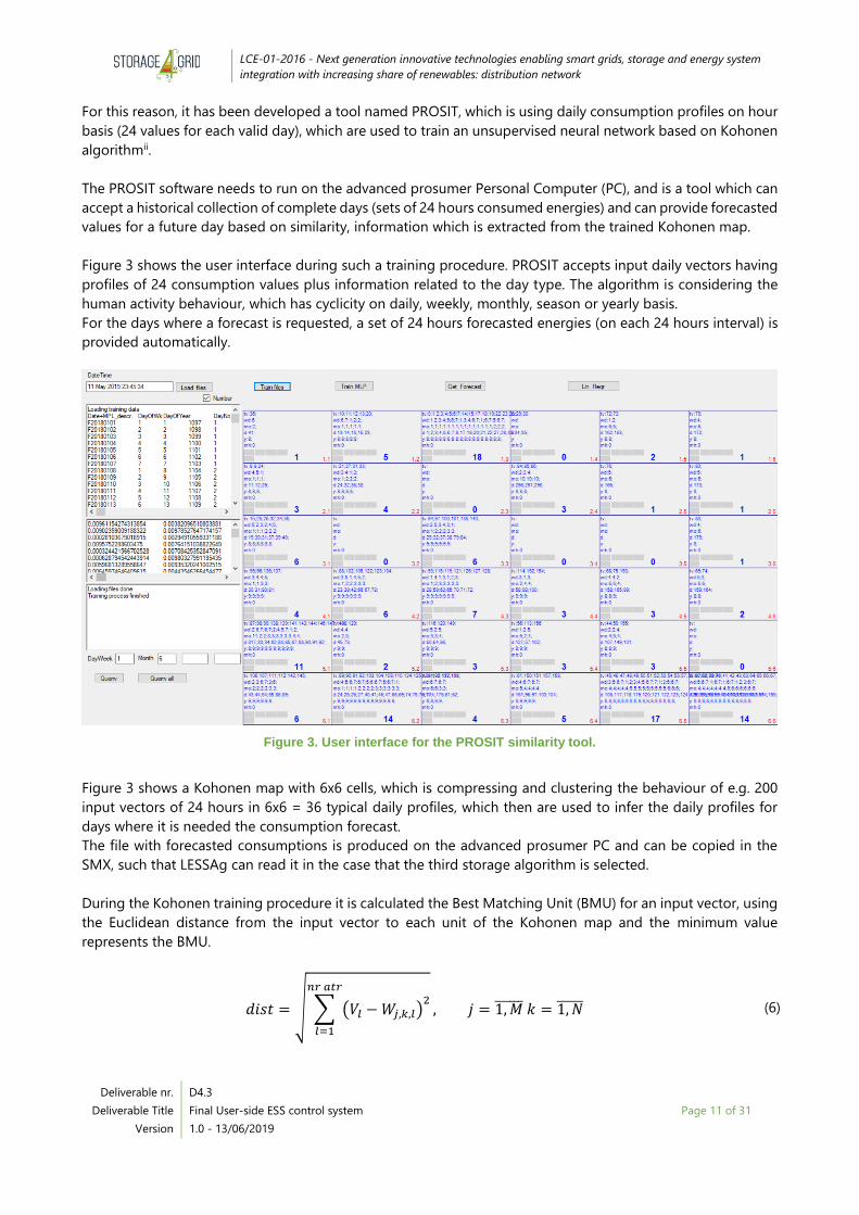
Figure 3 shows the user interface during such a training procedure. PROSIT accepts input daily vectors having

profiles of 24 consumption values plus information related to the day type. The algorithm is considering the

human activity behaviour, which has cyclicity on daily, weekly, monthly, season or yearly basis.

For the days where a forecast is requested, a set of 24 hours forecasted energies (on each 24 hours interval) is

provided automatically.

Figure 3. User interface for the PROSIT similarity tool.

Figure 3 shows a Kohonen map with 6x6 cells, which is compressing and clustering the behaviour of e.g. 200

input vectors of 24 hours in 6x6 = 36 typical daily profiles, which then are used to infer the daily profiles for

days where it is needed the consumption forecast.

The file with forecasted consumptions is produced on the advanced prosumer PC and can be copied in the

SMX, such that LESSAg can read it in the case that the third storage algorithm is selected.

During the Kohonen training procedure it is calculated the Best Matching Unit (BMU) for an input vector, using

the Euclidean distance from the input vector to each unit of the Kohonen map and the minimum value

represents the BMU.

𝑑𝑖𝑠𝑡 = √ ∑ (𝑉𝑙 − 𝑊𝑗,𝑘,𝑙)2

𝑛𝑟 𝑎𝑡𝑟

𝑙=1

, 𝑗 = 1, 𝑀̅̅ ̅̅ ̅̅ 𝑘 = 1, 𝑁̅̅ ̅̅ ̅ (6)



Deliverable nr.

Deliverable Title

Version

D4.3


1.0 - 13/06/2019

of 31

where V is the current input vector, W represents the values of the MxN map (6 x 6 map in the previous

example), each node containing as many attributes (referred as nr_atr in equation (6)) as the input vectors

contain.

During the training phase, the BMU and its neighbours are going to have their values updated. The

neighbourhood radius used in this method is:

𝜎 = 𝜎0exp (−

𝑖𝑡𝑒𝑟

𝜆) (7)

where “iter” is the current iteration, σ0 is half of the map dimension and λ is a constant calculated with the

relation:

𝜆 =

𝑖𝑡𝑒𝑟_𝑚𝑎𝑥

log(𝑠𝑖𝑔𝑚𝑎0) (8)

For more details on the algorithm, one can refer the classic book of Kohonen or other studies regarding the

Kohonen self-organized maps.

Figure 2 shows the interaction with SMX and the need to transfer the PROSIT output file in the SD card of SMX,

so it can be used by LESSAg in case of choosing the third algorithm.

2.2 PROFESS

PROFESS has had major advances since the first version of this deliverable [S4G-D4.2]. It works not only as

user-side ESS controller, but it is also designed and implemented to work together with Decision Support

Framework Simulation Engine (DSF-SE).

The main functionality of PROFESS is for using Model Predictive Control (MPC) in a real-time applicationiii. It

means, reading in real-time inputs, calculating an optimization problem and delivering outputs for the next

time step as set-points to the different south-bound connectors of the S4G system. It is important to mention

that some of these inputs have to be predicted for the optimization horizon being used. Examples of these

predictions constitute individual electric consumption (load) or PV generation for the next 24-hours.

Predictions are calculated inside PROFESS to guarantee data privacy and to cope with requirements of an

optimization problem.

2.2.1 Architecture

The PROFESS architecture is shown in Figure 4. The functionalities of each module were already described in

D4.2 [S4G-D4.2]. In this deliverable, solely updates during the last phase will be explained.



Deliverable nr.

Deliverable Title

Version

D4.3


1.0 - 13/06/2019

of 31

Figure 4. PROFESS architecture.

2.2.1.1 Sensor connector

Sensor connector (SC) and external devices connector (EDC) were fixed to use Sensor Measurement Lists (SenML)

data format as standard. In this way, information being delivered by sensors and the set-points calculated by

PROFESS can be easily linked to other components inside the S4G project. One example of this action is the

integration with ER in the Skive use case in Denmark as well as the integration of PROFESS with the DSF-SE.

For other components such as SMX, a dedicated connector was developed. This connector will be explained in

section 2.2.4.

2.2.1.2 External devices connector

The external devices connector (EDC) was enhanced with the possibility of delivering one or multiple set-points

as output. In order to explain it, it must be taken into consideration that this optimization problem is calculated

analysing the future of the system. This future is defined as a number of steps through the optimization horizon

separated a defined time step between them. In conclusion, the optimization will deliver outputs for the

optimization horizon being analysed.

In the first version of PROFESS, it was only included the possibility of delivering the result for the current time

step. This developed PROFESS into a provider of MPC to the system. Nevertheless, there are also situations

where the complete schedule for the optimization horizon is needed, e.g. inside the DSF-SE. This functionality

was added in this version through the outputs endpoint of the PROFESS-Application Program Interface (API)iv,

using the "horizon_values" flag. If true, the output of PROFESS consists of the complete calculated optimization

result. False, will deliver the current time step as an output.

2.2.1.3 Input and output data mapping

Inputs and outputs are registered exclusively via the inputs and outputs endpoints of the PROFESS-APIiv. This

registration is used internally in the framework to link the measured or predicted inputs to the inputs of the

optimization model. Similarly, the output registration is used to link the outputs of the optimization results to

the correct MQTT topic.



Deliverable nr.

Deliverable Title

Version

D4.3


1.0 - 13/06/2019

of 31

2.2.1.4 Optimization controller

Code in the central optimization controller (OC) was revised and bugs were corrected. The OC was especially

redesign to work with multiple optimization instances in the same platform. This development means working

with multi-processing and redefining the logs capability of the framework, in order to facilitate debugging.

2.2.1.5 Restriction mapping

The restriction mapping (RM) module was reconfigured to enable loading different optimization models to the

system. The modeler can use the models’ endpoint from the PROFESS APIiv to load any optimization model

that he or she developed using the mathematical framework Pyomov. The user can also give a name to this

model, which will be used to store it into the optimization model repository.

Once the user wants to run a model, he or she has to specifically link it using the optimization/start endpoint

under the flag "model_name".

2.2.1.6 Optimization modeller

The optimization modeller (OM) uses Pyomo as core tool for understanding the optimization models entered

by the user. From the models, OM can understand which are the data inputs and outputs needed for calculating

the optimization problem and wait for them. In fact, while all sets of inputs are not present as real-time data,

the controller cannot start any optimization calculation.

2.2.1.7 Mathematical solver

Solvers inside PROFESS were upgraded to the most recent versions. It includes GLPKvi, Ipoptvii and Bonminviii.

Moreover, a new solver for Mix Integer Problems (MIP) was added. Its name is CBCix.

Gurobix solver was also added to the system and can be linked only in AMD infrastructures using a floating

license running on a server. The developers are looking forward to testing it especially in PROFEV for the

stochastic dynamic programming running inside this platform.

2.2.2 Optimization algorithms

In this section, the different optimization algorithms used for three different optimization objectives in the

Fur/Skive use-cases will be presented. The schema and elements of the Fur/Skive use-case are presented in

Figure 5.

Figure 5. PROFESS residential scenario.



Deliverable nr.

Deliverable Title

Version

D4.3


1.0 - 13/06/2019

of 31

2.2.2.1 Inputs for the optimization problem

The optimization models require the inputs summarized in Table 1.

Table 1. Example inputs for the optimization model in Fur/Skive houses.

Input_name Value or MQTT params Description

ESS_Min_SoC 0.2 Minimum SoC that the

ESS can get

ESS_Max_SoC 0.9 Maximum SoC that the

ESS can get

SoC_Value

url 172.17.0.1

SoC value in real-time

being read from the ESS.

It is always between 0

and 1

topic con/opt/HOUSE_20/SoC_Value

qos 1

predict

ESS_Capacity 3600

ESS capacity in KWh

given by the producer

ESS_Max_Charge_Power 2400

Maximum power in Watt

for charging the ESS

given by the ESS inverter

ESS_Max_Discharge_Power 2400

Maximum power in Watt

for discharging the ESS

given by the ESS inverter

P_Grid_Max_Export_Power 6000 Maximum power in Watt

to export to the grid

P_PV

url 172.17.0.1

PV power in Watt in real-

time. It is always positive

topic con/opt/HOUSE_20/P_PV

qos 1

predict

PV_Inv_Max_Power 3120

Maximum PV power in

Watt that the PV can

generate

P_Load

url 172.17.0.1

Consumption power in

Watt in real-time. It is

always positive

topic con/opt/HOUSE_20/P_Load

qos 1

predict true



Deliverable nr.

Deliverable Title

Version

D4.3


1.0 - 13/06/2019

of 31

Some of them are constant values and others are real-time values read from the SenML connector or from the

Fronius South-bound connector as MQTT.

2.2.2.2 Optimization outputs

The optimization models provide the outputs summarized in Table 2. Outputs are delivered in different MQTT

topics.

Table 2. Example outputs for the optimization model in Fur/Skive houses.

Output_name MQTT params Description

P_Grid_Output

url 172.17.0.1

Power to be sent to the grid

or supplied by the grid. If

positive the power is

supplied by the grid.

topic output/P_Grid_Output

qos 1

unit W

horizon_steps false

P_PV_Output

url 172.17.0.1

PV power to be delivered to

the internal electric system.

It is always positive

topic output/P_PV_Output

qos 1

unit W

horizon_steps false

P_ESS_Output

url 172.17.0.1

Charging or discharging

power to or from the ESS. If

positive the ESS is

discharging.

topic output/P_ESS_Output

qos 1

unit W

horizon_steps false



Deliverable nr.

Deliverable Title

Version

D4.3


1.0 - 13/06/2019

of 31

2.2.2.3 Start configuration

For starting the PROFESS, configuration values of the optimization are required (Table 3).

Table 3. Configuration values of the optimization.

configs Value Description

control_frequency 60 Time step in seconds, in which the optimization

calculation is going to be repeated

horizon_in_steps 1440 Number of steps for the optimization horizon.

dT_in_seconds 60 Time in seconds between each horizon step.

repetition -1 Number of repetitions of the MPC. -1 means

infinitely

solver cbc Name of the solver to be used. Possibilities: GLPK,

Ipopt, Bonmin, CBC

Taking into consideration the optimization horizon (horizon_in_steps) of 1440 and the time between steps

(dT_in_seconds) of 60, the optimization inside PROFESS will be calculated for the next 24-hours with a

resolution of one minute.

2.2.2.4 Optimization constraints

The optimization model needs some constraints that describe the physical system and at the same time reduce

the solution space for the MIP problems. It is important to limit the maximal PV power that can be injected

into the system at any optimization time step:

𝑃𝑃𝑉𝑂𝑢𝑡𝑝𝑢𝑡≤ 𝑃𝑃𝑉𝐹𝑜𝑟𝑒𝑐𝑎𝑠𝑡

(9)

The PV output is given by the maximum power that a PV with certain surface and position can produce.

0 ≤ 𝑃𝑃𝑉𝑂𝑢𝑡𝑝𝑢𝑡≤ 𝑃𝑃𝑉_𝑀𝐴𝑋 (10)

The battery SoC is a state variable in this model, which is modelled as a function of the previous SoC and the

power exchange with the battery at the previous time step. Charging/discharging processes are assumed to

be 100% efficient. Inserting ∆𝑇

3600 term, the power exchange with the battery (kW) is translated into energy (kWs).

𝐸𝑏𝑎𝑡 is the battery’s energy storage capacity:

𝑆𝑜𝐶𝑡+1 = 𝑆𝑜𝐶𝑡 + 𝑃𝑏𝑎𝑡

∆𝑇

3600

1

𝐸𝑏𝑎𝑡

(11)

The power of the ESS is also limited by the maximum charging and discharging power that the ESS inverter

can support.

𝑃𝑏𝑎𝑡_𝑐ℎ𝑎𝑟𝑔𝑖𝑛𝑔_𝑚𝑎𝑥 ≤ 𝑃𝑏𝑎𝑡 ≤ 𝑃𝑏𝑎𝑡_𝑑𝑖𝑠𝑐ℎ𝑎𝑟𝑔𝑖𝑛𝑔_𝑚𝑎𝑥 (12)

The energy balance equation in the system is:

𝑃𝐿𝑜𝑎𝑑 = 𝑃𝑃𝑉𝑂𝑢𝑡𝑝𝑢𝑡+ 𝑃𝑏𝑎𝑡 + 𝑃𝐺𝑟𝑖𝑑 (13)



Deliverable nr.

Deliverable Title

Version

D4.3


1.0 - 13/06/2019

of 31

2.2.2.5 Objective functions

The constraints were used to model three different optimization objectives that the house owners can choose

using the residential GUI. The optimization problem is analysed for the defined horizon steps M.

The first one minimizes the amount of energy interchanged with the grid (𝑥𝐺𝑟𝑖𝑑). It means that the import of

energy as well as the export of it are minimized by the optimization algorithm.

𝑚𝑖𝑛𝑖𝑚𝑖𝑧𝑒 ∑ (𝑥𝐺𝑟𝑖𝑑

𝑚 )2

𝑀

𝑚=1

(14)

The second maximizes the utilization of the renewable potential, in this case the PV generation.

𝑚𝑎𝑥𝑖𝑚𝑖𝑧𝑒 ∑ 𝑃𝑝𝑣

𝑚 𝑥𝑝𝑣𝑚

𝑀

𝑚=1

(15)

And the third one minimizes the electricity bill using the energy price forecast (𝐶𝑝𝑟𝑖𝑐𝑒) obtained from the Energy

Price Connector of the S4G project, described in D5.4 [S4G-D5.4].

𝑚𝑖𝑛𝑖𝑚𝑖𝑧𝑒 ∑ 𝐶𝑝𝑟𝑖𝑐𝑒

𝑚 𝑥𝑔𝑟𝑖𝑑𝑚

𝑀

𝑚=1

(16)

2.2.3 Internal Load predictions

PROFESS requires for the optimization, predictions of the real-time inputs as e.g. consumption power (load)

and PV generation. The connector for PV generation prediction for PROFESS was already explained in D5.4

[S4G-D5.4]. Therefore, solely the model for load prediction will be explained in this deliverablexi.

A recurrent neural network (RNN) based on long short-term memory (LSTM) was used for load predictions

(Figure 6). This model was chosen for supporting long-term dependencies presented in the load data, which is

linked to seasonality and routine lifestyle of people. Moreover, LSTM supports an incremental learning of

incoming data, which is essential in our application. It creates the possibility of online learning while deployed

in the households without remote intervention.

From a high-level view, RNNs are a concatenation of multi-layer perceptions with equivalent processing units,

in order to process sequences using a non-linear function f:

𝑋 ∈ ℝ24×1, 𝑦′ ∈ ℝ24×1: 𝑓(𝑋) → 𝑦′ (17)

Figure 6. Incremental prediction/learning process.



Deliverable nr.

Deliverable Title

Version

D4.3


1.0 - 13/06/2019

of 31

In order to find the most optimal LSTM model to be implemented inside PROFESS, data of one house from an

open source dataset (OpenEI)xii was used. This data presents consumption profiles from different houses in the

USA for one-year (Figure 7). The idea was to obtain a model that can work robust and flexible with different

consumption datasets no matter their origin. In this way, the model was consequently evaluated with ten

further houses datasets of OpenEI and with five houses datasets of Fur/Skive, Denmark. The data of Fur/Skive

consists of three months consumption data in second resolution obtained during the execution of the S4G

project (Figure 8).

Figure 7. Consumption data of one House of OpenEI dataset.

Figure 8. Consumption data of one House in Fur/Skive, Denmark.

We proceeded analysing different configurations of LSTM to find the most optimal model in the predictions

for the next 24 hours. In fact, it was tested different hidden nodes, stack layers and joined it together with



Deliverable nr.

Deliverable Title

Version

D4.3


1.0 - 13/06/2019

of 31

dropout, regularization L1 and L2 and a mixture of dropout and regularization techniquesxiii. Results of the

analysis are presented in Table 4 as Mean Absolute Error (MAE) and Root Mean Squared Error (RSME) values.

Table 4: Analysis steps for choosing the optimal LSTM model.

Hidden

Layers

Number of

Nodes Regularization MAE (kW) RMSE

1 20 - 0,0651 0.0845

1 40 - 0,0377 0.0400

1 80 - 0,0471 0.0705

1 100 - 0,0321 0.0341

1 120 - 0,0355 0.0361

2 100 - 0,0576 0.0637

2 100 Dropout(0.1) 0,0345 0.0431

2 100 Dropout(0.2) 0,0311 0.0339

2 100 Dropout(0.3) 0,0299 0.0330

2 100 Dropout(0.4) 0,032 0.0349

2 100 Dropout(0.5) 0,1126 0.1741

2 100 Dropout(0.6) 0,032 0.0359

2 100 Dropout(0.7) 0,0392 0.0945

2 100 L1 (Alpha=0.01) 0,2291 0.2488

2 100 L2 (Alpha=0.01) 0,1217 0.1642

2 100 Dropout(0.3), L1

(Alpha=0.01) 0,2098 0.2343

2 100 Dropout(0.3), L2

(Alpha=0.01) 0,1945 0.2227

The best working model was the one with two stacked layers and a dropout of 0.3. Consequently, we evaluated

this model in the remaining nine houses of OpenEI and in the five houses of Fur/Skive. Table 5 shows the

results obtained with these datasets.



Deliverable nr.

Deliverable Title

Version

D4.3


1.0 - 13/06/2019

of 31

Table 5. Evaluation with OpenEI and Fur/Skive datasets.

Dataset HLayer Nodes Regularization MAE RMSE

openEI - 1 2 100 Dropout(0.3) 0,0299 0.0330

openEI - 2 2 100 Dropout(0.3) 0,0334 0.0371

openEI - 3 2 100 Dropout(0.3) 0,0701 0.1062

openEI - 4 2 100 Dropout(0.3) 0,0321 0.0353

openEI - 5 2 100 Dropout(0.3) 0,0314 0.0346

openEI - 6 2 100 Dropout(0.3) 0,0294 0.0319

openEI - 7 2 100 Dropout(0.3) 0,0331 0.0359

openEI - 8 2 100 Dropout(0.3) 0,0293 0.0322

openEI - 9 2 100 Dropout(0.3) 0,0314 0.0342

openEI - 10 2 100 Dropout(0.3) 0,0333 0.0369

Fur/Skive-1 2 100 Dropout(0.3) 0,0079 0.0091





The results showed a small MAE value of maximum 70 W with OpenEI Data. The data of Fur/Skive showed

better results obtaining a maximum MAE value of 8W during the predictions for the next 24-hours. It was also

analysed the training and prediction time. For Fur/Skive dataset the training time was 622 ± 46.8ms and the

prediction time was 4.49 ± 0.27ms.

Consequently, this model was translated into the PROFESS architecture and added it to a new container image

with name ML. This image is the one being linked to the optimization models in the Fur/Skive houses.

2.2.4 SenML connector

PROFESS uses SenMLxiv as standard for reading sensor data and publishing set-points to other software drivers.

Because in the S4G project no standard data model for smart meter measurements (SMX data) was defined,

we developed a connector that translates SMX-Data into the SenML standard.

This connector works similarly to PROFESS in a docker container, in order not to get problems with

dependencies of the host system.



Deliverable nr.

Deliverable Title

Version

D4.3


1.0 - 13/06/2019

of 31

The connector reads in the main thread data published by SMX in different topics of a broker. This data is

entered into a message queue, which is then read by different threads for changing the data format to SenML

standard. Afterwards, the data in SenML is published into the respective topic of the broker.

In order to define the broker and the topics where the SMX data is being published, a configuration file is

needed (see example below). This file also defines the meaning of the information inside a SMX data string

([KEYS]) and the broker and topic name where the new SenML data is going to be published ([IO]). An example

of a configuration file is further presented:

[IO]

channel = MQTT

mqtt.port = 1883

pub.mqtt.host = 172.17.0.1

pub.topic.prefix = con/opt/

[HOUSE_SMX_1]

sub.mqtt.host = 10.8.0.31

con.topic = {"topic":"EDYNA-0003/Data","qos":1}

[KEY_META]

level = 2

key.separator = /

[KEYS]

0-0-1-0-0-255/-2 = SMM_Time

1-1-32-7-0-255/-2 = U1

1-1-52-7-0-255/-2 = U2

1-1-72-7-0-255/-2 = U3

1-1-31-7-0-255/-2 = I1

1-1-51-7-0-255/-2 = I2

1-1-71-7-0-255/-2 = I3

1-1-36-7-0-255/-2 = P1

1-1-56-7-0-255/-2 = P2

1-1-76-7-0-255/-2 = P3

1-1-151-7-0-255/-2 = Q1

1-1-171-7-0-255/-2 = Q2

1-1-191-7-0-255/-2 = Q3

1-1-14-7-0-255/-2 = f

1-1-16-7-0-255/-2 = P

1-1-131-7-0-255/-2 = Q

1-1-1-8-0-255/-2 = Ap

1-1-2-8-0-255/-2 = Am

1-1-3-8-0-255/-2 = Rp

1-1-4-8-0-255/-2 = Rm

1-1-33-7-0-255/-2 = K1

1-1-53-7-0-255/-2 = K2

1-1-73-7-0-255/-2 = K3



Deliverable nr.

Deliverable Title

Version

D4.3


1.0 - 13/06/2019

of 31

3 Installation/Deployment instructions

3.1 LESSAg

LESSAg is a module which is embedded in the SMXcore package, thus taking full advantage of the environment

and modules which are offered by SMXcore. In this respect, for running LESSAg it is needed to run SMXcore

with a proper parameterisation.

In order to run SMXcore, it is needed to have the java environment installed in the SMX (as a Raspberry PI 3

Platform using Raspbianxv operating system), which is a feature usually available in Raspbian deployments.

In addition to other modules, it is needed to enable the modules needed for the advanced prosumer

application. The following specific modules need to be enabled: LESSAg and the MQTT client for

communication with the ER. The specific lines to enable the functionalities are further presented:

#

M6-Name=S4G_LESSAg

M6-ClassName=modules.contrib.S4G_LESSAg

M6-AttributesFile=S4G_LESSAg.txt

#

# Module MQTT client 2

#

#M1-Name=MQTTClient_ER

#M1-ClassName=modules.MQTTClient

#M1-AttributesFile=MQTTClient_ER.txt

#

To be noted that S4G_LESSAg.txt file is a parameterisation file which need to contain lines to instruct the

algorithm about its functionality, with keywords which have been presented in section 2.1.

The SMXcore will start with the same standard procedure used for obtaining the meter data readout with the

DLMS protocol, thus having an operational LESSAg in the same time with running the SMXcore application.

3.2 PROFESS

To prepare a SMXCore image it is necessary to follow the instructions document available to the consortium

[SmxGuide].

PROFESS uses a container architecture which simplifies its deployment. Images of the software are uploaded

into an open space of Docker Hubxvi. The user has to download the images and make them run into the final

platform (AMD or ARM). A complete installation guide is presented the Linksmart-Optimization Framework

web sitexvii.

In summary the installation consists in downloading the docker-compose file from the repository, pulling the

images and starting the container. The current docker-compose file is the following for ARM platforms:

version: '3.2'

services:

redis:

image: redis:latest

container_name: "redis_S4G"

command: redis-server

ports:

- "6379:6379"



Deliverable nr.

Deliverable Title

Version

D4.3


1.0 - 13/06/2019

of 31

restart: "always"

ofw:

image: garagon/optimization:arm

container_name: "ofw"

ports:

- "8080:8080"

depends_on:

- redis

volumes:

- ./optimization-framework/prediction/resources:/usr/src/app/prediction/resources

- ./optimization-framework/optimization/resources:/usr/src/app/optimization/resources

- ./optimization-framework/utils:/usr/src/app/utils

- ./optimization-

framework/utils/gurobi/license:/usr/src/app/share/gurobi811/license/gurobi.lic

command: ["python3", "-u", "ofw.py"]

restart: "always"

ml:

image: garagon/optimization:arm_training

container_name: "ml"

depends_on:

- redis

volumes:

- ./optimization-framework/prediction/resources:/usr/src/app/prediction/resources

command: ["python3", "-u", "mlTraining.py"]

restart: "always"

The command for pulling the image and starting the code is:

docker-compose -f {docker_compose_file_name} up –d

After this step, PROFESS is ready to run. The registry of inputs and outputs and the start command can be

entered through HTTP commands using the PROFESS API.

3.2.1 SenML Connector

Because the SenML connector works with docker, the installation procedure is similar to that of PROFESS. The

docker-compose file is the following:

version: '3.2' services: connector: image: garagon/optimization:arm_connector container_name: "connector" volumes: - ./optimization-framework/connector/resources/:/usr/src/app/connector/resources logging: driver: "json-file" options: max-size: "10m" max-file: "10" command: ["python3", "-u", "connectors.py"] restart: "always"

The command for pulling the image and starting the code is:

docker-compose -f {docker_compose_file_name} up –d



Deliverable nr.

Deliverable Title

Version

D4.3


1.0 - 13/06/2019

of 31

4 Software dependencies and requirements

No special hardware requirements are needed to implement the final version of the user-side ESS control.

The following sections describe the software dependencies of LESSAg and PROFESS.

4.1 LESSAg

The LESSAg prototype has the software dependencies described in Table 6.

Table 6. LESSAg software dependencies.

Dependency License Role

SMXCore GPL

Open source Core application

running in the trusted domain,

implementing the real-time

database, the communication with

SMM and with all extensions

running around SMXCore, by using

also a RBAC system to preserve

security and privacy for the used

data.

4.2 PROFESS

The PROFESS prototype has the software dependencies described in Table 7.

Table 7. PROFESS software dependencies.

Dependency License Role

Docker and docker-compose for

Raspbian Apache License 2.0

Docker is used to facilitate the

PROFESS installation.



Deliverable nr.

Deliverable Title

Version

D4.3


1.0 - 13/06/2019

of 31

5 API Reference

5.1 LESSAg

LESSAg is directly communicating with the real-time database of SMXcore and exchanging data with ER

through the dedicated ER MQTT client which is publishing and receiving data from the ER using the IEC 61850-

90-7 standard. This ER MQTT client is part of the ER SMX SB connector, detailed described in D4.9 [S4G-D4.9].

Moreover, the LESSAg outputs can be mapped to any specific MQTT topics, and in the current implementation,

they are mapped to the ER topics, since is the ER controlling the ESS interfaces.

As an example, the information regarding the battery SoC handled by the ER is obtained by subscribing with

the MQTT Client of SMXcore to the specific topic:

/ER/SMX/EnergyRouterInverter/ZBAT1.VolChgRte.instMag.f

which allows that specific payload with the desired information is received as MQTT message and finally that

battery SoC is copied in the SMXcore real-time database.

Similarly, the PV power exchanged can be obtained by subscribing to the topic:

/ER/SMX/EnergyRouterPV/MMDC1.Watt.instMag.f

while setting the reference power of the battery can be arranged by publishing the desired value in the

following MQTT topic:

/LESSAg/SMX/EnergyRouterInverter/ZBTC1.BatChaPwr.setMag.f

with the following SenML JSON format:

[

{

"v": 400.0,

"u": "W",

"t": 0,

"n": ""

}

]

used for the payload in order to set the power at the value 400 W.

In this way, there is no need for a direct API reference of LESSAg, but only MQTT messaging for publishing or

subscribing the values to be exchanged,

The data needed by LESSAg is grouped in the following classes:

• Data from the meter in the PCC;

• Data exchanged with the ER, according to the ER API interface, meaning set-points, operation modes

and instrumentation values;

• Data related to forecasts, which is obtained from the SD card, and transferred from outside, especially

from PROSIT and/or from the weather forecast services;

• Data for parameterisation, obtained from the parameterisation file.



Deliverable nr.

Deliverable Title

Version

D4.3


1.0 - 13/06/2019

of 31

Data needed by the prosumer for monitoring the process can be obtained through the MQTTClient, by using

the publish instructions of the main MQTT client module. A specific interface in GridMonK application has been

configured, while power grid environment is also simulated by using the OpenDSS load-flow program.

5.2 PROFESS

The PROFESS has been further developed in terms of functionalities and usability. Essential changes were made

in the last phase to increase its robustness and to allow the integration with other programs and services such

as the residential GUI and the DSF-SE. Figure 9 shows the current PROFESS API.

Figure 9. PROFESS API.



Deliverable nr.

Deliverable Title

Version

D4.3


1.0 - 13/06/2019

of 31

6 Conclusions

This document presents all the necessary information regarding the D4.3 - “Final User-side ESS control system”

prototypes (LESSAg and PROFESS), developed by the Storage4Grid project. No further updates of this

deliverable are expected. However, minor modifications and improvements might need to be

implemented/development during phase 3 integration and deployment actions.



Deliverable nr.

Deliverable Title

Version

D4.3


1.0 - 13/06/2019

of 31

Acronyms

Acronym Explanation

AMD Advanced Micro Devices

API Application Program Interface

BMU Best Matching Unit

DC Direct Current

DSF Decision Support Framework

DSF-SE Decision Support Framework Simulation Engine

EB Event Broker

EDC External Device Connector

EPRI Electrical Power Research Institute

ER Energy Router

ESS Energy Storage System

EV Electrical Vehicle

GESSCon Grid-side Energy Storage System Control

GridMonK Grid Monitoring and Control Knowledge

GPL General Public License

JSON JavaScript Object Notation

L-EMS Local Energy Management System

LESSAg Local Energy Storage System Agent

LSTM Long Short-Term memory

MAE Mean Absolute Error

ML Machine Learning

MPC Model Predictive Control

MQTT Message Queuing Telemetry Transport

MS Mathematical Solver

OC Optimization Controller

OM Optimization Modeller

OpenDSS Open Distribution System Simulator

PC Personal Computer

PCC Point of Common Coupling

PROFESS Professional Realtime Optimization Framework for Energy Storage Systems



Deliverable nr.

Deliverable Title

Version

D4.3


1.0 - 13/06/2019

of 31

PROSIT PROfiles SImiLarity Tool

PV Photovoltaics

RBAC Role-based Access Control

RM Restriction Mapping

RNN Recurrent Neural Network

RSME Root Mean Squared Error

S4G Storage4Grid

SB South-bound

SC Sensor Connector

SenML Sensor Measurement Lists

SMM Smart Metrology Meter

SMX Smart Meter eXtension

SoC State of Charge

USM Unbundled Smart Meter



Deliverable nr.

Deliverable Title

Version

D4.3


1.0 - 13/06/2019

of 31

List of figures

Figure 1. D4.3 prototype diagram [S4G-D3.2]. .......................................................................................................................................................... 6

Figure 2. LESSAg integration in the SMX architecture. .......................................................................................................................................... 7

Figure 3. User interface for the PROSIT similarity tool. ........................................................................................................................................ 11

Figure 4. PROFESS architecture. ..................................................................................................................................................................................... 13

Figure 5. PROFESS residential scenario. ..................................................................................................................................................................... 14

Figure 6. Incremental prediction/learning process. ............................................................................................................................................... 18

Figure 7. Consumption data of one House of OpenEI dataset. ....................................................................................................................... 19

Figure 8. Consumption data of one House in Fur/Skive, Denmark. ............................................................................................................... 19

Figure 9. PROFESS API. ...................................................................................................................................................................................................... 27

List of tables

Table 1. Example inputs for the optimization model in Fur/Skive houses. ................................................................................................. 15

Table 2. Example outputs for the optimization model in Fur/Skive houses. .............................................................................................. 16

Table 3. Configuration values of the optimization. ............................................................................................................................................... 17

Table 4: Analysis steps for choosing the optimal LSTM model. ....................................................................................................................... 20

Table 5. Evaluation with OpenEI and Fur/Skive datasets. ................................................................................................................................... 21

Table 6. LESSAg software dependencies.................................................................................................................................................................... 25

Table 7. PROFESS software dependencies. ............................................................................................................................................................... 25

References

i Sanduleac M., Cironei I., Albu M., Toma L., Sturzeanu M., Martins J., “Resilient Prosumer Scenario in a Changing Regulatory Environment - The UniRCon Solution,” Energies 2017, 10(12), 1941. ii Kohonen, T. (2001). Self-Organizing Maps. Third, Extended Edition. Springer Series in Information Sciences vol. 30, Berlin, Germany: Springer-Verlag, ISBN 978-3-540-67921-9. iii Seborg et al., “Process Dynamics and Control: Model Predictive Control,” pp. 414–438, 2011. iv Optimization Framework, API description, ttps://docs.linksmart.eu/display/LOF/API+Description v Pyomo, Python-based, open-source optimization modeling language, http://www.pyomo.org/, accessed 23 May 2019. vi GNU Linear Programming Kit, https://www.gnu.org/software/glpk/, accessed 13 May 2019. vii Introduction to IPOPT: A tutorial for downloading, installing, and using IPOPT, https://www.coin-or.org/Ipopt/documentation/, accessed 13 May 2019. viii Basic Open-source Nonlinear Mixed INteger programming, https://projects.coin-or.org/Bonmin, accessed 13 May 2019. ix Computational Optimization Infrastructure for Operations Research, COIN-OR Branch-and-Cut solver, https://github.com/coin-or/Cbc, accessed 13 May 2019. x Gurobi, The fastest mathematical programming solver, http://www.gurobi.com/, accessed 13 May 2019. xi Aragón G., Puri H., Grass A., Chala S., Beecks C., “Incremental Deep-Learning for Continuous Load Prediction in Energy Management Systems,” 2019, in press. xii Energy Information and Data | OpenEI, https://openei.org/, accessed 13 May 2019. xiii M. Ben Nasr and M. Chtourou, "On the training of recurrent neural networks," Eighth International Multi-Conference on Systems, Signals & Devices, Sousse, 2011, pp. 1-5. xiv Sensor Measurement Lists (SenML), https://tools.ietf.org/html/rfc8428, accessed 13 May 2019. xv Raspbian, free operating system based on Debian optimized for the Raspberry Pi hardware, https://www.raspbian.org/, accessed 23 May 2019. xvi Docker Hub, Build and ship any application anywhere, https://hub.docker.com/, accessed 23 May 2019. xvii Optimization Framework, Installation tutorial, https://docs.linksmart.eu/display/LOF/Installation, accessed 13 May 2019.

http://www.pyomo.org/

https://www.gnu.org/software/glpk/

https://www.coin-or.org/Ipopt/documentation/

https://www.coin-or.org/Ipopt/documentation/

https://projects.coin-or.org/Bonmin

https://github.com/coin-or/Cbc

http://www.gurobi.com/

https://openei.org/

https://tools.ietf.org/html/rfc8428

https://www.raspbian.org/

https://hub.docker.com/

https://docs.linksmart.eu/display/LOF/Installation

final user-side ess control system - storage4grid

Documents