evaluating emission benefits of a hybrid tug boat · evaluating emission benefits of a hybrid tug...

Evaluating Emission Benefits of a Hybrid Tug Boat

Final Report

October 2010

Prepared for:

Mr. Todd Sterling

California Air Resources Board

1001 I Street, Sacramento, CA 95814

Contract #07-413 and #07-419

Authors:

Ms. Varalakshmi Jayaram

Mr. M. Yusuf Khan

Dr. J. Wayne Miller

Mr. William A Welch

Dr. Kent Johnson

Dr. David R Cocker

University of California, Riverside

College of Engineering-Center for Environmental Research and Technology

Riverside, CA 92521

ii

Disclaimer

This report was prepared as the result of work sponsored by the California Air Resources

Board (CARB) and carried out with Foss Maritime Company. As such the report does not

necessarily represent the views of CARB and Foss Maritime Company. Further the

collective participants, its employees, contractors and subcontractors make no warrant,

express or implied, and assume no legal liability for the information in this report; nor

does any party represent that the uses of this information will not infringe upon privately

owned rights. This report has neither been approved nor disapproved by the collective

group of participants nor have they passed upon the accuracy or adequacy of the

information in this report.

iii

Acknowledgements

The authors would like to thank California Air Resources Board for their financial

support without which this project would not have been possible.

A special thanks to the following people for their time, effort and knowledge that helped

in the smooth progress of this project:

Foss Maritime Company

Susan Hayman and Elizabeth Boyd at the Seattle Office for coordinating and closely

following the progress of the project

Long Beach port engineers Jerry Allen, Jim Russell, Steve Harris and several crews on

the conventional and hybrid tugs for their logistical support during data acquisition and

emissions testing on the tugs.

Steve Hamil at the Seattle office for help with networking and setting up remote access

to the data acquisition system on the tugs.

Aspin Kemp & Associates

Chris Wright, Paul Jamer and others for providing signals from the batteries on the

hybrid boat and lengthy discussions on the operation and behavior of the batteries.

California Air Resources Board, El Monte

Edward Sun and Wayne McMahon for imparting their technical know-how on testing

hybrid and plug in vehicles.

Technical Working Group with members from California Air Resources Board, Foss

Maritime Company, Pacific Merchant Shipping Association, Ports of Los Angeles and

Long Beach, South Coast Air Quality Management District and U.S. Environmental

Protection Agency

For overseeing the progress of the project

Startcrest Consulting LLC

Galen Hon for his help in planning and installing the data acquisition system on the

tugs

Bruce Anderson and Mark Carlock for their inputs on development of the test protocol

Independent Contractors

Mac MacClanahan for developing a circuit board with relays to collect data from the

batteries on the hybrid boat.

College of Engineering-Center of Environmental Research and Technology (CE-CERT),

University of California Riverside

Charles Bufalino’s for his efforts in the emission test preparation

Kurt Bumiller for his help in developing the emissions data acquisition system

iv

Kathalena Cocker, Poornima Dixit, James Theodore Gutierrez, Sindhuja Ranganathan,

Letia Solomon, David Torres and Charles Wardle of the analytical laboratory for

preparation and analysis of filter sample media.

Alex Vu for his help in developing Python 2.6 code to analyze activity data and plot GPS

data.

Ed Sponsler for setting up a File Transfer Protocol (FTP) site to transfer data from the

tugs to CE-CERT.

v

Table of Contents

Disclaimer .......................................................................................................................... ii

Acknowledgements .......................................................................................................... iii

Table of Contents .............................................................................................................. v

List of Figures .................................................................................................................. vii

List of Tables .................................................................................................................... ix

Executive Summary .......................................................................................................... x

1 Introduction ............................................................................................................... 1

1.1 Project Objectives ................................................................................................ 2

2 Test Protocol and Test Plan ..................................................................................... 3

2.1 Overview .............................................................................................................. 3

2.2 Approach .............................................................................................................. 3

2.3 Test Boats ............................................................................................................. 4

2.4 Test Schedule ....................................................................................................... 7

2.5 Determining Tug Boat Activity............................................................................ 8

2.5.1 Tug Operating Modes ................................................................................... 8

2.5.2 Data Logging Procedure ............................................................................. 10

2.5.3 Establishing Weighing Factors for Tug Operating Modes ......................... 17

2.5.4 Developing Engine Histograms .................................................................. 19

2.5.5 Calculating the Average Load Required for a Tug Operating Mode .......... 23

2.6 Emissions Testing Procedure ............................................................................. 23

2.6.1 Test Engines ................................................................................................ 23

2.6.2 Fuels ............................................................................................................ 25

2.6.3 Test Cycle and Operating Conditions ......................................................... 26

2.6.4 Sampling Ports ............................................................................................ 28

2.6.5 Measuring Gases and PM2.5 emissions ....................................................... 30

2.6.6 Calculating Exhaust Flow Rates ................................................................. 30

2.6.7 Calculation of Engine Load ........................................................................ 31

2.6.8 Calculation of Emissions in g/hr ................................................................. 31

2.6.9 Calculation of Emission Factors in g/kW-hr .............................................. 31

3 Results and Discussions .......................................................................................... 33

3.1 Activity ............................................................................................................... 33

3.1.1 Weighing Factors for Tug Operating Modes .............................................. 33

3.1.2 Engine Histograms for Conventional Tug .................................................. 36

3.1.3 Engine Histograms for Hybrid Tug ............................................................ 38

3.1.4 Engine Histograms for Hybrid Tug without Batteries ................................ 42

3.2 Emissions Testing .............................................................................................. 45

3.2.1 Test Fuel Properties .................................................................................... 45

3.2.2 Emissions Testing Phase 1 .......................................................................... 45

3.2.3 Emissions Testing Phase 2 .......................................................................... 51

3.2.4 Carbon Balance ........................................................................................... 57

3.3 Total In-Use Emissions ...................................................................................... 58

4 Summary and Recommendations .......................................................................... 64

References ........................................................................................................................ 66

vi

Appendix A - Measuring Gaseous & Particulate Emissions ..................................... A-1

A.1 Scope…………………………………………………………………………A-2

A.2 Sampling System for Measuring Gaseous and Particulate Emissions………..A-2

A.3 Dilution Air System…………………………………………………………..A-3

A.4 Calculating the Dilution Ratio………………………………………………..A-5

A.5 Dilution System Integrity Check……………………………………………..A-5

A.6 Measuring the Gaseous Emissions: CO, CO 2, HC, NOx, O2, SO2 …A-5

A.6.1 Measuring Gaseous Emissions: ISO & IMO Criteria…………………….A-5

A.6.2 Measuring Gaseous Emissions: UCR Design…………………………….A-6

A.7 Measuring the Particulate Matter (PM) Emissions…………………A-8

A.7.1 Added Comments about UCR’s Measurement of PM…………………...A-8

A.8 Measuring Real-Time Particulate Matter (PM) Emissions-DustTrak…

…………………………………………………………………………..A-9

A.9 Quality Control/Quality Assurance (QC/QA)…………………… ..A-10

Appendix B - Test Cycles and Fuels for Different Engine Applications .................. B-1

B.1 Introduction…………………………………………………………………...B-2

B.1.1 Intermediate speed………………………………………………………..B-2

B.2 Engine Torque Curves and Test Cycles………………………………………B-3

B.3 Modes and Weighting Factors for Test Cycles……………………………….B-3

Appendix C - Tug Boat Specifications ........................................................................ C-1

C.1 Conventional Tug……………………………………………………………..C-2

C.2 Hybrid Tug……………………………………………………………………C-3

Appendix D – Engine Specifications from Manufacturers ....................................... D-1

D.1 Main Engine on Conventional Tug…………………………………………...D-2

D.2 Auxiliary Engine on Conventional Tug………………………………………D-8

D.3 Main Engine on Hybrid Tug………………………………………………...D-10

D.4 Auxiliary Engine on Hybrid Tug……………………………………………D-13

Appendix E – Fuel Analysis Results ............................................................................ E-1

vii

List of Figures

Figure ES- 1 Overall In-Use Emissions based on Individual Tug Operating Mode

Weighing Factors ........................................................................................ xi

Figure 2-1 Diesel Electric Drive Train on the Hybrid Tug ................................................. 6

Figure 2-2 Schematic of Data Logging System on the Conventional Tug ....................... 13

Figure 2-3 Schematic of the Data Logging System on the Hybrid Tug ........................... 14

Figure 2-4 Data-Logger, USB-1608FS and Relays on the Hybrid Tug ........................... 15

Figure 2-5 USB2-4COM-M - Receives serial signals from four engines and transmits

them through one USB port to the data-logger .......................................... 15

Figure 2-6 Dearborn Protocol Adapter ............................................................................. 16

Figure 2-7 Wheelhouse on the Hybrid Tug shows Wheelhouse Switch in Orange

Rectangle .................................................................................................... 16

Figure 2-8 ECM Load versus CO2 Emissions for the Conventional Tug Main Engine

CAT 3512 C ............................................................................................... 20

Figure 2-9 ECM Load versus CO2 Emissions for the Conventional Tug Auxiliary Engine

JD 6081 AFM75 ......................................................................................... 20

Figure 2-10 ECM Load versus CO2 Emissions for the Hybrid Tug Main Engine Cummins

QSK50-M ................................................................................................... 21

Figure 2-11 ECM Load versus CO2 Emissions for the Hybrid Tug Auxiliary Engine

Cummins QSM11-M .................................................................................. 21

Figure 2-12 Correlation between Engine Load and Engine Speed for the Conventional

Tug Main Engine CAT 3512 C .................................................................. 22

Figure 2-13 Auxiliary Engine on Conventional Tug JD 6085 .......................................... 24

Figure 2-14 Main Engine on Hybrid Tug Cummins QSK50-M ....................................... 25

Figure 2-15 Auxiliary Engine on Hybrid Tug QSM11-M ................................................ 25

Figure 2-16 Schematic of Test Setup for Phase 2 Emissions Testing .............................. 28

Figure 2-17 Sampling Port for Main Engine on Hybrid Tug............................................ 29

Figure 2-18 Sampling Port for Auxiliary Engine of Hybrid Tug ..................................... 29

Figure 3-1 Overall Weighing Factors for Tug Operating Modes ..................................... 33

Figure 3-2 Dock Locations in the Port of Los Angeles and Long Beach ......................... 35

Figure 3-3 GPS data of a typical day for the Conventional Tug ...................................... 35

Figure 3-4 Main Engine Histograms for Conventional Tug ............................................. 37

Figure 3-5 Engine Histogram for Hybrid Tug-1 ............................................................... 38

Figure 3-6 Engine Histograms for the Hybrid Tug-2 ....................................................... 40

Figure 3-7 Engine Histograms for the Hybrid Tug-3 ....................................................... 41

Figure 3-8 Engine Histograms for Hybrid Tug without Batteries - 1 ............................... 42

Figure 3-9 Engine Histograms the Hybrid Tug without Batteries -2................................ 43

Figure 3-10 Engine Histograms for the Hybrid Tug without Batteries -3 ........................ 44

Figure 3-11 Emission Factors for Main Engine on Conventional Tug CAT 3512C ........ 48

Figure 3-12 Emission Factors for Auxiliary Engine on Conventional Tug JD 6081 ....... 48

Figure 3-13 Emission Factors for Main Engine on Hybrid Tug Cummins QSK50-M .... 49

Figure 3-14 Emission Factors for Auxiliary Engine on Hybrid Tug QSM11-M ............. 49

Figure 3-15 PM2.5 Mass Balance for A)Main Engine Conventional Tug CAT 3512 C

B)Auxiliary Engine Conventional Tug JD 6081 C) Main Engine Hybrid

viii

Tug Cummins QSK50-M D) Auxiliary Engine Hybrid Tug Cummins

QSM11-M .................................................................................................. 50

Figure 3-16 Comparison of Phases 1 & 2 for Main Engine on Conventional Tug CAT

3512 C ........................................................................................................ 53

Figure 3-17 Comparison of Phases 1 & 2 for Main Engine of Hybrid Tug Cummins

QSK50-M ................................................................................................... 54

Figure 3-18 Comparison of Phases 1 & 2 for Auxiliary Engine on Hybrid Tug Cummins

QSM11-M .................................................................................................. 55

Figure 3-19 Emissions Profile for Main Engine on Conventional Tug CAT 3512 C ...... 56

Figure 3-20 Emissions Profile of Main Engine on Hybrid Tug QSK50-M ...................... 56

Figure 3-21 Emissions Profile of Auxiliary Engine on Hybrid Tug Cummins QSK11-M

.................................................................................................................... 57

Figure 3-22 Carbon Balance for Test Engines .................................................................. 58

Figure 3-23 Overall Emission Reductions ........................................................................ 61

Figure 3-24 Overall Emission Reductions for Retrofit Scenario 1 ................................... 62

Figure 3-25 Overall Emission Reductions for Retrofit Scenario 2 ................................... 63

Figure A-1 Partial Flow Dilution System with Single Venturi, Concentration

Measurement and Fractional Sampling .................................................... A-3

Figure A-2 Field Processing Unit for Purifying Dilution Air in Carrying Case ............. A-3

Figure A-3 Setup Showing Gas Analyzer with Computer for Continuous Data Logging ...

.................................................................................................................... A-6

Figure A-4 Picture of TSI DustTrak ............................................................................... A-9

Figure B-1 Torque as a Function of Engine Speed ......................................................... B-3

Figure B-2 Examples of Power Scales............................................................................ B-3

ix

List of Tables

Table 2-1 Engine Specifications for Conventional Tug ..................................................... 5

Table 2-2 Engine Specifications for Hybrid Tug ................................................................ 5

Table 2-1 Data Logging Test Schedule .............................................................................. 7

Table 2-2 Test Schedule for Emissions Testing Phases 1 and 2 ......................................... 8

Table 2-3 Operating Details for Conventional Tug ............................................................ 9

Table 2-4 Operating Details for Hybrid Tug ...................................................................... 9

Table 2-5 Details of Data-Logger ..................................................................................... 12

Table 2-8 Engine Specifications for Conventional Tug ................................................... 24

Table 2-9 Engine Specifications for Hybrid Tug .............................................................. 24

Table 2-8 Test Matrix for Emissions Testing Phase 1 ...................................................... 27

Table 2-9 Test Matrix for Emissions Testing Phase 2 ...................................................... 27

Table 3-1 Weekly Variation in Operating Mode Weighing Factors for Conventional Tug

......................................................................................................................... 34

Table 3-2 Weekly Variation in Operating Mode Weighing Factors for Hybrid Tug ....... 34

Table 3-3 Selected Fuel Properties ................................................................................... 45

Table 3-4 Results for Phase 1 of Emissions Testing in g/hr ............................................. 46

Table 3-5 Emission Factors in g/kW-hr from Phase 1 of Testing .................................... 47

Table 3-6 Results of Phase 2 of Emissions Testing .......................................................... 52

Table 3-7 Average Load Requirements for Each Operating Mode .................................. 58

Table 3-8 Emission Factors for Shore Power17, 18

............................................................. 59

Table 3-9 Modal and Overall Emission Reductions with Hybrid Technology ................ 61

Table 3-10 Modal and Overall Emissions Reductions with Hybrid Technology for

Retrofit Scenario 1 .......................................................................................... 62

Table 3-11 Modal and Overall Emissions Reductions with Hybrid Technology for

Retrofit Scenario 2 .......................................................................................... 63

Table A-1 Components of a Sampling System: ISO/IMO Criteria & UCR Design ...... A-4

Table A-2 Detector Method and Concentration Ranges for Monitor ............................. A-7

Table A-3 Quality Specifications for the Horiba PG-250 .............................................. A-7

Table A-4 Measuring Particulate by ISO and UCR Methods ......................................... A-8

Table B-1 Definitions Used Throughout ISO 8178-4..................................................... B-2

Table B-2 Combined Table of Modes and Weighting Factors ....................................... B-4

x

Executive Summary

Background: Modern mobile sources are expected to simultaneously reduce criteria

pollutants and greenhouse gas emissions to address the issues of air quality and global

warming. One prevalent technology solution to achieve this goal is the use of two or

more propulsion sources commonly known as the hybrid technology. Calculating the

emissions benefits of a hybrid technology is quite challenging. The common thread in

developing new test protocols is to ensure that energy used from multiple sources is

properly analyzed. The goal of this research was to develop and implement a new test

protocol that quantifies the benefits of using hybrid technology for a tugboat. For this

purpose a side by side comparison of two “dolphin class” tugs, one conventional and the

other hybrid, operating in the Ports of Los Angeles and Long Beach was performed. The

conventional tug was powered by four diesel engines while the hybrid tug operated on

four diesel engines and 126 batteries. All engines met United Stated Environmental

Protection Agency’s Tier 2 certification.

Methods: This research project was conducted in three stages. The first stage involved

development of a data-logging system capable of simultaneously monitoring and

reporting the status of the power sources on each tug. This system was installed for a

period of one month on each tug. Gigabytes of data were analyzed to determine the

weighing factors, i.e., the fraction of time spent by the tug in the six discrete operating

modes shore power, dock, transit, ship assist and barge move. Further engine histograms

for all eight engines at these operating modes were established. A small sample of

activity data (~1.5 days) was collected on the hybrid tug operating without batteries to

quantify the effects of the diesel electric drive train versus batteries on the total emission

reductions. The second stage of the research was a two-phase emissions testing program

that focused on establishing an emissions profiles of the diesel engines. Emissions of

criteria pollutants – nitrogen oxide, carbon monoxide, particulate matter and greenhouse

gas carbon dioxide were measured based on the ISO 8178 protocols. The final stage of

the research involved combining the activity and emissions data to calculate the overall

in-use emissions from each tug and the emission reductions with the hybrid technology.

Results: The individual weighing factors at each operating mode for both tugs were

found to be in good agreement. The average weighing factors for these operating modes

were found to be 0.54 for dock plus shore power, 0.07 for standby, 0.17 for transit, 0.17

for ship assist and 0.05 for barge move. The conventional tug did not plug into shore

power while the hybrid tug spent one-third of the time at dock plugged into shore power.

During this program the batteries were not charged by shore power.

Detailed engine histograms for all eight engines at each operating mode are presented in

the body of the report. The average operating loads as a percentage of the maximum

power rating of the engines were found to be: 16% and 12% for the main and auxiliary

engine on the conventional tug. 12% and 34% for the main and auxiliary on the hybrid

tug. Detailed emissions profile data for one auxiliary and one main engine on each tug

were obtained. Results are provided in Section 3.2.3 of the report.

xi

Figure ES-1 shows the overall in-use emissions for each tug based on the individual

operating mode weighing factors. Emission reductions with the hybrid technology were

found to be 73% for PM2.5, 51% for NOx and 27% for CO2. The fuel equivalent CO2

reductions were within 5% of the fuel savings reported by the tug owner over an eight

month period. The diesel electric drive train on the hybrid tug that allows the use of

auxiliary power for propulsion was the primary cause for the overall in-use emission

reductions as opposed to the batteries. The transit operating mode was the most

significant contributor to the overall emission reductions. A couple of retrofit scenarios

for hybridization of existing tugs were modeled.

Figure ES- 1 Overall In-Use Emissions based on Individual Tug

Operating Mode Weighing Factors

Conclusions:

An activity based model was developed to estimate the overall in-use emission

reductions of a hybrid tug boat.

Tug boats are a good application for the hybrid technology. Significant emission

reductions were observed: 73% for PM2.5, 51% for NOx and 27% for CO2.

The average operating load of the engines on both tugs are well below the load

factors specified in the standard ISO duty cycles. The finding indicates need for the

development of in-use duty cycle that would increase the accuracy of emission

inventories.

The hybrid system increased the average operating load on the auxiliary engine from

12% to 34%. However, the average load on the main engines was found to be only

12% of the maximum rating. These engines are still operating in inefficient zone

suggesting the need for a larger energy storage system and smaller main engines in

the next generation of hybrid tugs.

Further improvements will result when the plug-in version is operative.

44.1

30.9

20.8

13.216.8 16.9

12.115.3 15.3

0

10

20

30

40

50

PM2.5 Nox/10 CO2/10000

Ove

rall

In-U

se E

mis

sio

ns

(g/h

r)

Conventional Tug Hybrid Tug without Batteries Hybrid Tug

NOx/10 CO2/10000PM2.5

1

1 Introduction The last decade has seen an increasing interest in the emissions from marine sources.

Several studies1-6

have shown that emissions from ports significantly affect the air quality

in the populated areas around them. The sources in the ports include ships, harbor-craft,

cargo-handling equipment, trucks and locomotives. Ships are the largest contributors to

the total port emissions. Emissions from harbor-craft, though smaller, still form a

significant part of the total port emissions7, 8

. Harbor crafts include ferries, excursion

boats, tugboats, towboats, crew and supply vessels, work boats, fishing boats, barges and

dredge vessels.

Corbett’s study9 on waterborne commerce vessels in the United States revealed that in

several states ~65% of the marine nitrogen oxide comes from vessels operating in inland

waterways. Since, harbor craft (e.g., barges and tow-boats) are the most common

commercial vessels operating in inland waterways10

they could have significant effects

on the air quality of inland areas as well.

Harbor-craft are typically powered by marine compression ignition engines which are

regulated by United States Environmental Protection Agency’s (U.S. EPA) code of

federal regulation title 40 parts 85-9411

. Emission studies12, 13

on these vessels have

predominately focused on older engines operating on high sulfur fuels. Current EPA

emissions for these new marine engines require the use of low sulfur (<500ppm S) diesel

or ultra-low sulfur diesel (ULSD) (<15ppm S).

Future regulations are geared towards simultaneous reduction of toxic air contaminants,

criteria pollutants and green-house gas emissions to address the issues of air quality and

global warming. One prevalent technology solution to achieve this goal is the use of two

or more propulsion sources also known as the hybrid technology. A common application

of this technology today is passenger cars.

This technology is not new to the marine world. Diesel electric submarines have been

prevalent for over sixty years. The propeller (usually single) on these submarines is

driven by an electric motor which derives energy from diesel generators or batteries. The

diesel generators were also used to charge batteries.

Calculating the emissions benefits of a hybrid technology is quite challenging as they

operate quite differently from the conventional technology. Test protocols developed for

conventional systems have to be adapted appropriately based on the application. The

common thread in developing new test protocols is to ensure that energy used from

multiple sources is properly analyzed. The goal of this research was to develop and

implement a new test protocol that quantifies the benefits of using hybrid technology for

a tugboat.

2

1.1 Project Objectives

The primary goal of this project is to develop and implement a test protocol that

establishes the emission reduction potential of the hybrid technology on a tug boat. Listed

below are the different steps involved in achieving this goal

Determine the activity of the tug boat by establishing typical operating modes,

weighing factors and engine histograms for each of these modes.

Measure gaseous and particulate matter (PM2.5) emissions from the main and auxiliary engines on the tug boats to

o Verify if the engines meet the EPA Tier 2 standard during their typical

operation.

o Determine the emissions profile of these engines that can be coupled with

the activity data to calculate their total in-use emissions in g/hr.

Combining the activity and emissions data to determine the difference between the total emissions from a hybrid and conventional tug boat.

3

2 Test Protocol and Test Plan

2.1 Overview

The primary goal of this project is to determine the emission benefits of using a hybrid

system on a tug. For this purpose two tugs from Foss Maritime Company’s fleet, the Alta

June (conventional tug) and the Carolyn Dorothy (hybrid tug), were chosen. Both tugs

are “dolphin class” vessels equipped with four EPA Tier 2 certified engines.

Listed below is a brief description of the procedure adopted to determine the in-use

emission benefits of the hybrid tug.

a) Engine, GPS and battery data were logged for a month from each tug. This data

was analyzed to determine the activity of the tugs and engine histograms for each

operating mode.

b) In-use emission measurements were made on one main and one auxiliary engine

on each tug. These engines were analyzed to determine the gaseous (CO, CO2 and

NOx) and particulate matter (PM2.5) emissions for each engine across that

engine’s entire operating range.

c) Activity and engine histogram data coupled with the emissions data were used to

determine the total in-use emissions in g/hr from each tug.

d) These total in-use emissions were then used to calculate the reduction of the

gaseous and particulate matter species with the hybrid technology.

A detailed description of the approach, test schedule, measurement and analyses

techniques used to determine the emission reduction potential of the hybrid technology

are provided below.

2.2 Approach

The emission benefits of a hybrid tug can be calculated as follows

---------- Equation 2-1

where,

total in-use emissions for conventional tug in g/hr

total in-use emissions for hybrid tug in g/hr

The total in-use emissions of any gaseous or particulate matter species, is determined

using the following equation:

---------- Equation 2-2

where,

total in-use emissions in g/hr

4

total number of operating modes (Section 2.5.1)

the total number of power sources on the tug (Section 2.3)

weighting factor for operating mode (See Equation 2-3)

total in-use emissions in g/hr from the power source for the operating

mode (See Equation 2-4)

The weighing factors for each operating mode are calculated as follows:

---------- Equation 2-3

where,

weighing factor for the operating mode

time spent by the tug in the operating mode

total sample time for the tug

As mentioned earlier, tug boats typically have four engines, two for propulsion and two

auxiliary generators. To determine the total in-use emissions from each of these

engines/power sources the following equation can be used:

----------Equation 2-4

where,

total in-use emissions in g/hr from the power source/engine for the

operating mode

total number of operating modes for the power source (marine diesel engine).

there are twelve operating modes for the engine based on the percentage of

maximum engine load: off, 0 to <10%, 10% to <20%, 20% to <30%, and so on

until 90% to <100% and 100%.

fraction of time spent by the power source/engine at its operating mode

during the tug boat operating mode. This value can be obtained from the

engine histograms

emissions in g/hr for the power source/engine at its operating mode

While developing engine histograms for the hybrid tug it is important to ensure that the

state of charge of the battery at the start and end time of each sample period chosen for

the calculation of the engine histogram are the same. This would eliminate any biases in

emissions resulting from operation of the auxiliary generators for charging the batteries.

The protocol was adopted after reviewing the hybrid testing protocol adopted by the

Society of Automotive Engineers14

(SAE) and California Air Resources Board 15

(CARB)

for testing hybrid electric vehicles.

2.3 Test Boats

The primary goal of this project is to determine the emissions benefits of using a hybrid

technology on a tug boat. For this purpose two boats, Alta June (conventional) and

Carolyn Dorothy (hybrid), belonging to Foss Maritime Company’s fleet operating in the

5

Ports of Los Angeles and Long Beach were chosen. Both tugs were equipped with EPA

Tier 2 certified marine diesel engines. Vessel information is provided in Appendix C.

Details of power sources on these boats are described below.

The conventional tug is powered by two 1902 kW CAT 3512C main engines and two 195

kW John Deere 6081 auxiliary engines (Table 2-1). This tug has two propellers. Each

main engine is connected through a mechanical drive shaft to one propeller. Therefore

both main engines have to be operated for moving and maneuvering the boat. The

auxiliary engines are used for hotelling, lighting, air conditioning and operating the winch

motor.

Table 2-1 Engine Specifications for Conventional Tug

Main Engine Auxiliary Engine

Manufacturer /Model CAT 3512C John Deere 6081 AFM75

Manufacture Year 2008 2008

Technology 4-Stroke Diesel 4-Stroke Diesel

Max. Power Rating 1902 kW -

Prime Power - 195 kW

Rated Speed 1800 rpm 1800 rpm

# of Cylinders 12 6

Total Displacement 58.6 lit 8.1 lit

The hybrid tug is powered by two 1342 kW Cummins QSK50-M main engines and 317

kW Cummins QSM11-M auxiliary generators (Table 2-2). It also has 126 soft gel lead

acid batteries for power storage that are separated into two arrays with 63 batteries each.

Each array stores 170.1kW-hr of energy when fully charged.

Table 2-2 Engine Specifications for Hybrid Tug


Manufacturer /Model Cummins QSK50-M Cummins QSM11-M




Prime Power - 317 kWm


# of Cylinders 16 6

Total Displacement 50 lit 10.8 lit

Figure 2-1 shows the diesel electric drive train on the hybrid tug. As in the case of the

conventional tug the main engines are linked mechanically to the propellers through a

6

drive shaft. However, there is a motor-generator unit mounted on the shaft between each

engine and propeller. This unit allows the electrical power from the batteries and

auxiliary engines to drive the shaft for propelling the boat. Therefore the main engines on

the hybrid tug have lower power rating than the ones on the conventional.

The motor generator also provides electrical power generated from the shaft using the

main engines or freewheeling propeller (regenerative power) which is used for charging

the batteries, driving the winch and other hotelling activities of the tug.

The batteries on the tug are predominately charged using the power from the auxiliary

engines drawn through the DC bus. Since these auxiliary engines are used for charging

batteries and propelling the boat, they have a higher power rating than those on the

conventional tug.

The batteries have the capability of being charged by shore power. During this test

program sufficient shore power was not available at the port to charge the batteries. As a

result the batteries were always charged using the auxiliary engines.

The hybrid tug is equipped with an energy management system that manages the power

sources and the drive train. The captain on the hybrid tug uses a switch in the wheelhouse

to communicate the current operating mode of the tug to the energy management system.

The signal from this wheelhouse switch helps the energy management system in making

decisions regarding the number of power sources required to operate the tug. Further

details of this wheelhouse switch are provided is Section 2.5.2.

Figure 2-1 Diesel Electric Drive Train on the Hybrid Tug

Auxiliary Engine

Propeller

Main Engine

Motor Generator

DC Bus

Battery Array

7

2.4 Test Schedule

The testing program was conducted in over a seven month period from January to July

2010. The testing consists of two parts

a) Data Logging for a one month period on each tug to determine tug activity

b) Emissions testing of one main and one auxiliary engine on each tug.

Table 2-1 shows the data logging schedule for the conventional and the hybrid tugs.

During data logging on the hybrid tug several problems were encountered with the data-

logger and the tug boat. As a result data was obtained intermittently for five to sixteen

day periods instead of one continuous one month period. In the final phase of data

logging, the hybrid tug was operated for a period of 1.5 days (06/14/2010 09:00 to

06/15/2010 23:00), with the batteries disconnected from the diesel electric drive train.

This was done to determine the effects of the drive train versus the batteries on the

overall emission reductions. Details of the data logging procedure and analysis to

determine the tug activity are provided in Section 2.5.

Table 2-3 Data Logging Test Schedule

Tug Boat Start Time End Time

Conventional 1/8/2010 17:04:41 2/12/2010 13:10:22

Hybrid

3/4/2010 17:24:32 3/21/2010 4:59:58

3/26/2010 14:45:40 4/2/2010 10:30:53

4/30/2010 8:19:46 5/11/2010 11:53:23

5/19/2010 9:52:13 5/24/2010 8:14:29

6/8/2010 10:02:04 6/17/2010 12:22:25

Emissions testing of one main and one auxiliary engine on each tug were performed in

two phases. A brief description of these phases is provided below. Further details on

emissions testing and analysis are presented in Section 2.6.

Phase 1 involved in-use gaseous and PM2.5 emissions measurements based on the ISO

8178-1 protocol following the load points in the standard certification cycle. The main

propulsion engines were tested based on the ISO 8178-4 E3 cycle and the auxiliary

engines were tested following the ISO 8178-4 D2 cycle.

Phase 2 of emissions testing involved determining an emissions profile of the main

engines on both tugs and the auxiliary engine on the hybrid tug. For this purpose gaseous

and real time PM2.5 emissions were measured across several load points spanning the

entire operating range of the engines.

8

Phase 1 was performed during the initial stages of data logging on each tug while Phase 2

was conducted at the end of the test program. Table 2-2 shows the emissions test

schedule.

Table 2-4 Test Schedule for Emissions Testing Phases 1 and 2

Phase Tug Boat Engine Date Start Time End Time

1

Conventional JD 6081 01/14/10 09:00 17:30

CAT 3512C 01/15/10 08:30 17:30

Hybrid Cummins QSM11-M 03/03/10 09:00 17:00

Cummins QSK50-M 03/04/10 09:00 17:30

2

Conventional CAT 3512 C 07/08/10 10:00 16:30

Hybrid Cummins QSM11-M 06/08/10 11:00 13:45

Cummins QSK50-M 06/08/10 13:45 17:30

2.5 Determining Tug Boat Activity

The following sections describe the typical operating modes of the tug boat, procedure

for data collection and analysis to establish the weighing factors for each operating mode

as well as development of engine histograms for all four engines on each tug.

2.5.1 Tug Operating Modes

After several conversations with port engineers and executives from the tug company the

modes of operation of a typical tug were determined. These are provided below:

Shore Power: The tug is at the dock plugged into shore power for its utilities. None of the

engines are operating during this mode. The hybrid boat spends considerable amount of

time plugged into shore power while the conventional tug hardly plugs in.

Dock: During this operation the tug boat is at the dock with one auxiliary engine

operating for powering the lights and air-conditioning on the boat. On the conventional

tug one auxiliary engine is on at dock. The hybrid tug switches between one auxiliary

engine and batteries during this mode. If the state of charge (SOC) of the battery arrays

reduce to 60% one of the auxiliary engines turn on to charge the batteries and provide

hotelling power for the tug. As soon as the batteries are charged to a SOC of 80% the

engine turns off and the batteries discharge providing hotelling power.

Standby: In this mode the tug is idling in the water waiting for a call from the pilot or

dispatch to start or transit to a job. The conventional tug operates two main propulsion

engines and one auxiliary generator during standby. As in the case of dock the hybrid tug

switches between the batteries and one auxiliary engine.

9

Transit: This mode refers to the movement of the tug between jobs and to and from

different docks. The conventional tug boat operates two main engines and one auxiliary

engine during transit. The hybrid boat switched between batteries and one auxiliary

engines for transit at slow speed <6.0 knots within the port. For higher speeds the hybrid

tug operates two auxiliary generators.

Ship Assist and Barge Moves Tug boats typically perform two kinds of jobs in the ports –

a) assisting ships from berth to sea and vice-versa b) moving barges from one location to

another. Each of these jobs is treated as a separate operating mode as the total work done

for ship assist and barge move are considerably different. The conventional tug operates

two main engines and one auxiliary engine during this mode. The hybrid boat operates all

four engines for a job. Also one battery array is on the charging mode and the other is in

the discharge mode.

Tables 2-3 and 2-4 show the operating details for the conventional and hybrid tug boats

during each mode

Table 2-5 Operating Details for Conventional Tug

Operational

Modes

ME #1

CAT 3512

ME #2

CAT 3512

AE #1

JD 6081

AE#2

JD 6081

Shore Power Off Off Off Off

Dock Off Off On Off

Standby On On On Off

Transit On On On Off

Barge Move On On On Off

Ship Assist On On On Off

ME: Main Engine, AE: Auxiliary Engine

Table 2-6 Operating Details for Hybrid Tug

Operational

Modes

ME #1 Cummins

QSK50-M

ME #2 Cummins

QSK50-M

AE #1 Cummins

QSM11-M

AE#2 Cummins

QSM11-M

Battery

Shore Power Off Off Off Off Off

Dock Off Off On Off On

Standby Off Off On Off On

Transit Off Off On Off On

Fast Transit Off Off On On On

Barge Move On On On On On

Ship Assist On On On On On

ME: Main Engine, AE: Auxiliary Engine

10

2.5.2 Data Logging Procedure

To determine the activity of the conventional and hybrid tug GPS, engine and battery

data had to be logged continuously for a period of one month from each tug. For this

purpose, a Labview program was developed that was capable of interfacing with four

engine electronic control modules (ECMs), a GPS and batteries to retrieve the required

information continuously on a second by second basis and write it into a comma

separated value (CSV) file. Each line in the CSV file generated by the code represents

one second. The program automatically creates a new file after 65500 seconds thereby

ensuring that the CSV file is not too large for Microsoft Excel to handle. This Labview

program was installed and operated on the data-logger which is a standard laptop with

Windows XP operating system. Table 2-7 lists all the parameters that were logged from

the two tugs along with the devices used for interfacing between the power sources and

the data-logger.

Schematics of the data-logger set up on the conventional and hybrid boats are provided in

Figures 2-2 and 2-3. The data-logger was placed on the workbench in the engine room of

each tug boat. Data from the ECMs on the two main propulsion engines and the two

auxiliary engines were obtained using four Dearborn Protocol Adapters that convert the

J1939 signals to serial/RS-232 signals. Power for the Dearborn adapters was obtained

from the batteries used for engine startup.

A Garmin GPS that provides data on location, speed and course of the tug at any second

during the sample time was placed at the top of the mast on the tug boat to ensure that it

receives a clear signal. Serial cables were run from GPS to the data-logger.

An event-logger developed by Starcrest Consulting LLC, was installed in the wheelhouse

of the conventional tug. This event-logger is a circular switch that provides a distinct

analog voltage signal for each position that it is on. These switch positions were used to

indicate the operating modes as follows,

Position 1 - 3.0 volts - Dock

Position 2 - 4.5 volts - Standby

Position 3 - 6.0 volts - Slow Transit, speed < 6.0 knots (speed limit in the port)

Position 4 - 7.5 volts - Fast Transit, speed > 6.0 knots

Position 5 - 9.0 volts - Assist

The Captains on the tug were provided with instructions on operating the event-logger

switch. The analog signal from the event-logger was transmitted through shielded cables

to the data-logger in the engine room.

The hybrid tug is operated differently from the conventional tug. It has a switch in the

wheelhouse that used by the captains for operating the boat. This wheelhouse switch

communicates with an energy management system to determine how many power

sources will be required for that operation. The wheelhouse switch has four positions which indicate the mode of operation of the tug. These are listed below:

1 - Dock Tug switches between the batteries and one auxiliary engine.

2 - Standby Tug switches between the batteries and one auxiliary engine.

11

3 - Transit Tug uses one or two auxiliary engines along with batteries

depending on the load requirement.

4 - Assist Tug uses all four engine and the batteries for a job.

Aspin Kemp and Associates provided us with five digital signals, four from the

wheelhouse switch and one indicating if the boat was plugged into shore power or not.

They also provided us with six analog signals that give information on the operation of

the two battery arrays

1 - State of Charge of Array A

2 - State of Charge of Array B

3 - Voltage of Array A

4 - Voltage of Array B

5 - Current for Array A

6 - Current for Array B

Remote access was made available by Foss Maritime Company using Virtual Network

Computing (VNC) server and client application. UCR was able to log onto the data-

logger on a daily basis to ensure that the system was operating properly. The wireless

network on the boat was not strong enough for file transfer. Therefore the port engineer

uploaded the CSV files and scanned copies of the tug’s paper logs on a weekly basis to a

file transfer protocol (FTP) site.

12

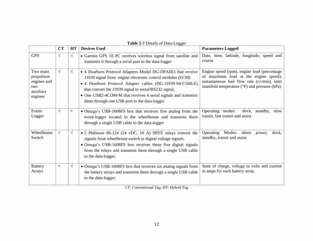
Table 2-7 Details of Data-Logger

CT HT Devices Used Parameters Logged

GPS √ √ Garmin GPS 18 PC receives wireless signal from satellite and

transmits it through a serial port to the data-logger

Date, time, latitude, longitude, speed and

course

Two main

propulsion

engines and

two

auxiliary

engines

√ √ 4 Dearborn Protocol Adapters Model DG-DPAIII/i that receive

J1939 signal from engine electronic control modules (ECM)

4 Dearborn Protocol Adapter cables (DG-J1939-04-CABLE)

that convert the J1939 signal to serial/RS232 signal,

One USB2-4COM-M that receives 4 serial signals and transmits

them through one USB port to the data-logger

Engine speed (rpm), engine load (percentage

of maximum load at the engine speed),

instantaneous fuel flow rate (cc/min), inlet

manifold temperature (°F) and pressure (kPa)

Event-

Logger

√ × Omega’s USB-1608FS box that receives five analog from the

event-logger located in the wheelhouse and transmits them

through a single USB cable to the data-logger

Operating modes: dock, standby, slow

transit, fast transit and assist

Wheelhouse

Switch

× √ 5 Philmore 86-124 (24 vDC, 10 A) SPDT relays convert the

signals from wheelhouse switch to digital voltage signals.

Omega’s USB-1608FS box receives these five digital signals

from the relays and transmits them through a single USB cable

to the data-logger.

Operating Modes: shore power, dock,

standby, transit and assist

Battery

Arrays

× √ Omega’s USB-1608FS box that receives six analog signals from

the battery arrays and transmits them through a single USB cable

to the data-logger.

State of charge, voltage in volts and current

in amps for each battery array.

CT: Conventional Tug, HT: Hybrid Tug

13

Figure 2-2 Schematic of Data Logging System on the Conventional Tug

Port Main Engine

2008 CAT 3512 C

1902kW

Starboard Main Engine

2008 CAT 3512 C

1902kW

Data-Logger

Laptop

Labview

Program

DB

2

DB

3D

B1

DB

4

Event

Logger

RS

23

2 t0

US

B

GPS

US

B 1

60

8 F

S

J1939

J1939

J1939

J1939

RS

-23

2RS

-23

2

RS

-23

2

RS-232

US

BUS

B

An

alo

g

RS

-23

2

USB

RS-232

Starboard

Auxiliary Engine

JD 6081 AFM75

195kW

Port Auxiliary

Engine

JD 6081 AFM75

195kW

DB: Dearborn Adapter

14

Figure 2-3 Schematic of the Data Logging System on the Hybrid Tug

Port Main Engine

2007 Cummins QSK50-M

1342kW

Starboard Main Engine

2007 Cummins QSK50-M

1342 kW

Battery

Array A

Data-Logger

Laptop Labview

Program

DB

2

DB

3D

B1

DB

4

Switch

RS

232 t0 U

SB

GPS

US

B 1

608 F

S

J1939

J1939

J1939

J1939

RS

-23

2

RS

-23

2

RS

-23

2

RS-232

US

BUS

B

USB

RS-232

Analog

Analog

Analog

SOC

Volts

Amps

Battery

Array B

Analog

Analog

Analog

SOC

Volts

Amps

Shore Power

Dock

Idle

Transit

Assist

Digital

Digital

Digital

Digital

Digital

DB: Dearborn Adapter

SOC: State of Charge

Starboard

Auxiliary Engine

Cummins QSK11

317kWm

Port Auxiliary

Engine

Cummins QSK11

317kWm

15

Figure 2-4 Data-Logger, USB-1608FS and Relays on the Hybrid Tug

Figure 2-5 USB2-4COM-M - Receives serial signals from four

engines and transmits them through one USB port to the data-logger

16

Figure 2-6 Dearborn Protocol Adapter

Figure 2-7 Wheelhouse on the Hybrid Tug shows Wheelhouse Switch in Orange Rectangle

17

2.5.3 Establishing Weighing Factors for Tug Operating Modes

The weighing factor for each operating mode was calculated as the ratio of the time spent

by the tug in that mode to the total sample time (Equation 2-3). The CSV files obtained

from the data-logger have a field called “opmode” that contained a unique number/code

for each tug operating mode based on the data obtained from the event-logger switch for

the conventional tug and the wheelhouse switch for the hybrid tug.

During the analysis several discrepancies were seen in the data obtained from the

switches on both tugs. These had to be rectified before calculating the weighing factors.

Details of these corrections are provided below.

Conventional Tug: On this tug, the human error involved in turning the event-logger

switch made the signal from the event-logger unreliable. As a result data from the boats

paper logs, engines and GPS had to be analyzed to determine the operation mode. This

was done as follows. The opmode field on each line in the CSV files contained a unique

code to indicate the operating mode 1-Ship Assist, 2-Barge Move, 3-Shore Power, 4-

Dock, 5-Standby and 6-Transit. Here is how the operating modes were determined.

The boat’s paper logs provide accurate start time, end time and route for ship

assists and barge moves. So based on these logs the codes 1 or 2 were manually

entered into opmode field of the CSV files

At times when the tug was not performing a ship assist or barge move the

following filters were used

o When all four engines are off the tug is plugged into shore power

o When both main engines are off tug is at the dock

o If the GPS speed is greater than 0.0 knots and both main engines are on,

the tug is in transit

o If the GPS speed is 0.0 knots and at least one main engines is on, the tug

is in standby

Hybrid Tug: As in the case of the conventional tug the wheelhouse switch on the hybrid

tug was not accurate. Listed below are some instances which resulted in inaccuracy:

Typically the tug is switched to transit mode 2-5 minutes before the beginning of

transit. These few minutes belong to the standby mode.

When the time between two transits is less than fifteen minutes the tug is

operated in transit mode instead of switching back and forth between standby and

transit.

When the time between two jobs is small (<20 minutes) the tug transits from one

job to the next on the assist mode.

In the event the tug has to rush to get to a job, the tug is operated on the assist

mode. This provides extra power for fast transit.

Some captains switch to assist mode 5-15 minutes before the job begins. So the

tug could be in the last part of its transit to the job or on standby when the switch

is on assist mode.

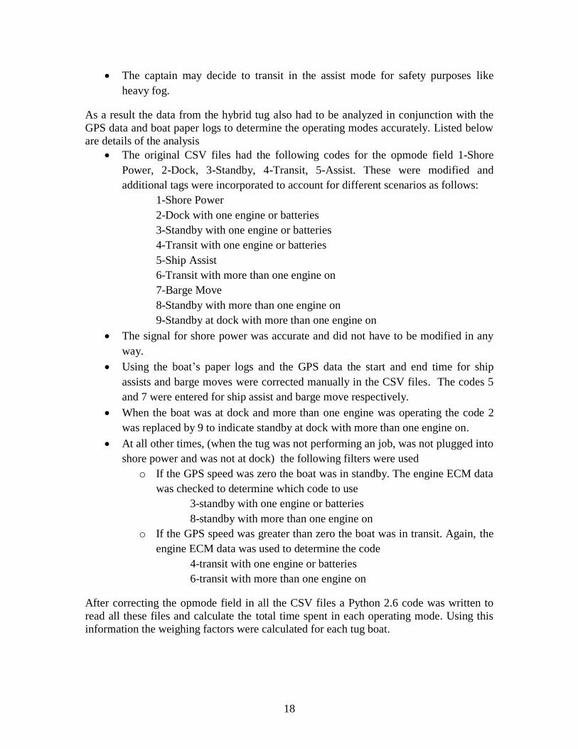
18

The captain may decide to transit in the assist mode for safety purposes like

heavy fog.

As a result the data from the hybrid tug also had to be analyzed in conjunction with the

GPS data and boat paper logs to determine the operating modes accurately. Listed below

are details of the analysis

The original CSV files had the following codes for the opmode field 1-Shore

Power, 2-Dock, 3-Standby, 4-Transit, 5-Assist. These were modified and

additional tags were incorporated to account for different scenarios as follows:

1-Shore Power

2-Dock with one engine or batteries

3-Standby with one engine or batteries

4-Transit with one engine or batteries

5-Ship Assist

6-Transit with more than one engine on

7-Barge Move

8-Standby with more than one engine on

9-Standby at dock with more than one engine on

The signal for shore power was accurate and did not have to be modified in any

way.

Using the boat’s paper logs and the GPS data the start and end time for ship

assists and barge moves were corrected manually in the CSV files. The codes 5

and 7 were entered for ship assist and barge move respectively.

When the boat was at dock and more than one engine was operating the code 2

was replaced by 9 to indicate standby at dock with more than one engine on.

At all other times, (when the tug was not performing an job, was not plugged into

shore power and was not at dock) the following filters were used

o If the GPS speed was zero the boat was in standby. The engine ECM data

was checked to determine which code to use

3-standby with one engine or batteries

8-standby with more than one engine on

o If the GPS speed was greater than zero the boat was in transit. Again, the

engine ECM data was used to determine the code

4-transit with one engine or batteries

6-transit with more than one engine on

After correcting the opmode field in all the CSV files a Python 2.6 code was written to

read all these files and calculate the total time spent in each operating mode. Using this

information the weighing factors were calculated for each tug boat.

19

2.5.4 Developing Engine Histograms

Engine histograms are basically graphs showing the amount of time the engine spends at

different loads. In this project engine histograms have to be developed for all four

engines on each tug for each tug operating mode. During the data logging procedure the

engine speed in rpm and engine load as a percentage of the maximum load at that speed

were retrieved from the engines’ ECMs and written into the CSV files. For the auxiliary

engines which are constant speed diesel generators, the percent load from the ECM has to

be multiplied by the maximum rated load of the engine in kW to get the load on the

engine. The main propulsion engines are variable speed engines. Therefore, at any given

speed the maximum attainable load in kW was obtained from the engines’ lug curve and

multiplied by the percent load retrieved from the ECM to determine the load on the

engine. Lug curves for these main engines (CAT 3512 C, Cummins QSK50-M) were

obtained from the respective engine manufacturer (Appendix D).

Engine ECMs do not actually measure the load on the engine; they use an algorithm to

estimate the load. This algorithm is proprietary and varies from one engine manufacturer

to another. Typically engine ECMs provide an accurate load estimate at high engine loads

and deviate from the true value at low loads. This is true particularly for off-road and

marine engines where ECMs are not regulated.

The ratio of the carbon-dioxide emissions to the load on the engine is an indication of its

thermal efficiency. This efficiency tends to be relatively constant across the entire range

of engine operation. Therefore we would expect a straight line relationship between the

engine load and the CO2 emissions in g/hr. Any significant deviation from the straight

line relationship will indicate an error in the load readings provided by the ECM. Figures

2-8, 2-9, 2-10 and 2-11 show plots of engine ECM load versus the measured CO2

emissions in kg/hr for one auxiliary and one main engine on each tug. A good straight

line correlation is observed for all but the main engine on the conventional tug (CAT

3512 C). For this engine we see that the load drops off from the straight line around the

25% engine load. Therefore a load correction has to be applied to this engine alone.

The data-logger used on the conventional tug collected engine speed and percent

maximum load from the engine ECM. It does not collect a real-time CO2 emissions data.

Therefore the equation for the straight line fit to the ECM load versus CO2 cannot be used

to correct this data. Instead the load has to be presented as a function of the engine speed.

Figure 2-12 shows the correlation between the CO2 corrected engine load and engine

speed for the CAT 3512 C engine. This correlation was used to calculate the load for

speeds below 1300rpm, for all higher speed the percent load obtained from the ECM was

used for the calculation.

20

Figure 2-8 ECM Load versus CO2 Emissions for the

Conventional Tug Main Engine CAT 3512 C


Conventional Tug Auxiliary Engine JD 6081 AFM75

y = 1.42x

R² = 1.00

0

500

1000

1500

2000

2500

0 500 1000 1500

En

gin

e E

CM

Lo

ad

(k

W)

CO2 Emissions (kg/hr)

y = 1.29x

R² = 1.00

0

30

60

90

120

150

0 50 100 150

En

gin

e E

CM

Lo

ad

kW


21


Hybrid Tug Main Engine Cummins QSK50-M


Hybrid Tug Auxiliary Engine Cummins QSM11-M

y = 1.23x

R² = 1.00

0

200

400

600

800

1000

1200

1400

0 500 1000 1500

En

gin

e E

CM

Lo

ad

(k

W)


y = 1.30x

R² = 0.98

0

50

100

150

200

250

0 50 100 150 200

Lo

ad

kW


22

Figure 2-12 Correlation between Engine Load and Engine

Speed for the Conventional Tug Main Engine CAT 3512 C

Microsoft Excel was used for the calculation of the engine loads. Four extra fields were

added in the CSV files for the calculated loads of the main and the auxiliary engines.

Engine loads were then split into twelve bins:

Bin Off Engine is Off

Bin 1 0 to <10%

Bin 2 10% to <20%

Bin 3 20% to <30%

Bin 4 30% to <40%

Bin 5 40% to <50%

Bin 6 50% to <60%

Bin 7 60% to <70%

Bin 8 70% to <80%

Bin 9 80% to <90%

Bin 10 90% to <100%

Bin 11 100%

Four more fields were added to indicate the bin in which the main and auxiliary engines

were operating. A Python 2.6 code was written to calculate the total time spent by the

engine in each bin for each operating mode. Using this data the fraction of time spent by

the engine in any bin for a particular operating mode was calculated. This was then

plotted in the form of engine histograms.

The engine histograms developed from the CSV files are used to calculate the total

emissions from a tug. Therefore it is important to ensure that the state of charge of the

y = -1.64E-06x3 + 5.31E-03x2

- 4.50E+00x + 1.30E+03

R² = 9.99E-01

0

200

400

600

800

1000

0 500 1000 1500

CO

2C

orr

ecte

d E

ng

ine

Lo

ad

(k

W)

Engine Speed (rpm)

23

battery at the start and end time of each sample period chosen for the calculation of the

engine histogram are the same. This would eliminate any biases in emissions resulting

from the use of the auxiliary engine for charging the batteries. This protocol was adopted

based on the guidelines in the SAE14

and CARB15

testing protocols for hybrid electric

vehicles.

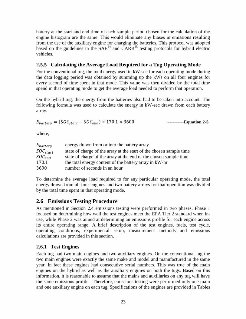
2.5.5 Calculating the Average Load Required for a Tug Operating Mode

For the conventional tug, the total energy used in kW-sec for each operating mode during

the data logging period was obtained by summing up the kWs on all four engines for

every second of time spent in that mode. This value was then divided by the total time

spend in that operating mode to get the average load needed to perform that operation.

On the hybrid tug, the energy from the batteries also had to be taken into account. The

following formula was used to calculate the energy in kW-sec drawn from each battery

array.

----------Equation 2-5

where,

energy drawn from or into the battery array

state of charge of the array at the start of the chosen sample time

state of charge of the array at the end of the chosen sample time

the total energy content of the battery array in kW-hr

number of seconds in an hour

To determine the average load required to for any particular operating mode, the total

energy drawn from all four engines and two battery arrays for that operation was divided

by the total time spent in that operating mode.

2.6 Emissions Testing Procedure

As mentioned in Section 2.4 emissions testing were performed in two phases. Phase 1

focused on determining how well the test engines meet the EPA Tier 2 standard when in-

use, while Phase 2 was aimed at determining an emissions profile for each engine across

its entire operating range. A brief description of the test engines, fuels, test cycle,

operating conditions, experimental setup, measurement methods and emissions

calculations are provided in this section.

2.6.1 Test Engines

Each tug had two main engines and two auxiliary engines. On the conventional tug the

two main engines were exactly the same make and model and manufactured in the same

year. In fact these engines had consecutive serial numbers. This was true of the main

engines on the hybrid as well as the auxiliary engines on both the tugs. Based on this

information, it is reasonable to assume that the mains and auxiliaries on any tug will have

the same emissions profile. Therefore, emissions testing were performed only one main

and one auxiliary engine on each tug. Specifications of the engines are provided in Tables

24

2-8 and 2-9. Pictures of some of the test engines are provided in Figures 2-13, 2-14 and

2-15.

Table 2-8 Engine Specifications for Conventional Tug


Manufacturer /Model CAT 3512C John Deere 6081 AFM75




Prime Power - 195 kW


# of Cylinders 12 6

Total Displacement 58.6 lit 8.1 lit

Table 2-9 Engine Specifications for Hybrid Tug


Manufacturer /Model Cummins QSK50-M Cummins QSM11-M




Prime Power - 317 kWm


# of Cylinders 16 6

Total Displacement 50 lit 10.8 lit

Figure 2-13 Auxiliary Engine on Conventional Tug JD 6085

25

Figure 2-14 Main Engine on Hybrid Tug Cummins QSK50-M

Figure 2-15 Auxiliary Engine on Hybrid Tug QSM11-M

2.6.2 Fuels

All four engines were tested while operating on the normal fuel of operation, red dye

ultra low sulfur diesel. A fuel sample was obtained from each tug and sent to an external

26

laboratory for analysis of selected properties. Details of the fuel analysis are provided in

Table 3-3 in the results section.

2.6.3 Test Cycle and Operating Conditions

Phase 1: The primary goal of this phase of the testing program was to establish if the test

engines meet their certification standards when in-use. Gaseous and PM2.5 emission

measurements on these engines were made based on the ISO 8178-1 protocol (Appendix

A). Briefly, a partial dilution system with a venturi was used for PM2.5 sampling

(Appendix A, Figure A-1). Carbon dioxide, nitrogen oxides and carbon monoxide were

measured in both the raw and the dilute exhaust. The ratio of the concentration of carbon

dioxide in the raw to the in the dilute was used to determine the dilution ratio for PM2.5

sampling.

The main propulsion engines were tested following the steady state load points in the ISO

8178-4 E3 cycle. An additional measurement was made at the idle load. The auxiliary

engines were operated at the steady state load points in the ISO 8178-4 D2 cycle. Details

of the test cycles are provided in Appendix B.

The steady state load points on the main engine of the conventional tug and both engines

on the hybrid tug were achieved while the tug pushed against the pier. The auxiliary

engine on the hybrid tug could not be operated at loads higher than 75%. Also for loads

<20% the engine would keep switching on and off due to the presence of the batteries.

Hence these low loads could not be measured.

Since the auxiliary generator on the conventional tug is not used for propulsion and the

typical steady state load on this engine is 12% of its maximum load, a load bank had to

be used to achieve the higher load points. Even with the load bank this engine could not

be operated steadily at loads higher than 75%. Therefore only four out of the five load

points on the D2 cycle were achieved for emissions testing.

Due to practical considerations, the actual engine load at each test mode on all four

engines could differ by a factor of ±5% from the ISO target load. Table 2-8 lists the test

matrix for Phase 1 of emissions testing.

At each steady state test mode the protocol requires the following:

Allowing the gaseous emissions to stabilize before measurement at each test mode.

Measuring gaseous and PM2.5 concentrations for a time period long enough to get measurable filter mass

Recording engine speed (rpm), displacement, boost pressure and intake manifold temperature in order to calculate the mass flow rate of the exhaust.

27

Table 2-10 Test Matrix for Emissions Testing Phase 1

Tug Boat Engine Date Engine Loads

Conventional JD 6081 01/14/10 RT & ISO: 75%,50%,25%, 10%

CAT 3512C 01/15/10 RT & ISO: 100%,75%,50%,25%, Idle

Hybrid Cummins QSM11-M 03/03/10 RT & ISO: 75%, 50%, 25%

Cummins QSK50-M 03/04/10 RT & ISO: 100%, 75%, 50%, 25%, Idle

RT: Real Time Monitoring and Recording of Gaseous Emissions

ISO: Filter Samples taken in accordance with ISO 8178-4 E3/D2 cycles

Phase 2: The goal of Phase 2 was to determine the emissions profile of the test engines

over their entire operating range. The activity data showed that auxiliary engine on the

conventional tug operates at a steady load of 12%, since this load point was already tested

during Phase 1 this engine was not tested again. The other three test engines had a wider

range of operating conditions. The loads on the auxiliary engine of the hybrid tug varied

from idle to 75% of the prime power. The main engines on both tugs operated

predominantly at the low loads and occasionally at loads at high as the maximum rated

power. The test matrixes for all three engines were designed to incorporate the steady

state load points already measured during Phase 1 along with several intermediate steady

state loads (Table 2-9). This matrix will fill in some of the gaps between the ISO target

loads and provide a better idea of the emission trends for each engine as a function of its

load.

Table 2-11 Test Matrix for Emissions Testing Phase 2

Tug Boat Engine Date Engine Speeds (rpm)/ Load (% max)

Conventional CAT 3512C 07/08/10 RTP: 1780, 1655, 1542, 1434, 1301, 1142,

1000, 900, 800, 700, Idle

Hybrid

Cummins

QSM11-M 06/08/10 RTP: 75%, 60%, 50%, 40%, 25%, 20%

Cummins

QSK50-M 06/08/10

RTP: 1780, 1700, 1600, 1525, 1424, 1300,

1142, 1050, 950, 850, 750, Idle

RTP: Real Time Monitoring and Recording of Gaseous and PM2.5 Emission

Gaseous measurements were made in accordance to the ISO 8178-1 protocols (Appendix

A, Section A.6). A simple partial dilution system was used for measuring the real-time

PM2.5 emissions using TSI’s DustTrak (Appendix A, Section A.8). Schematic of this test

setup is shown in Figure 2-16. As in the case of Phase 1, gaseous measurements were

made both in the raw and dilute exhaust. The ratio of the CO2 concentrations in the raw

versus the dilute was used to determine the dilution ratio for PM2.5 measurements.

28

At each steady state test mode the following were done:

Allowing the gaseous emissions to stabilize before measurement at each test mode.

Measuring gaseous and PM2.5 concentrations for a total time of five minutes.

Recording engine speed (rpm), displacement, boost pressure and intake manifold temperature in order to calculate the mass flow rate of the exhaust.

Figure 2-16 Schematic of Test Setup for Phase 2 Emissions Testing

2.6.4 Sampling Ports

Only one sample port was available in the stack of each engine. A T- joint was installed

at the end of the sample probe to provide raw gas sample for gaseous measurements and

dilution for PM2.5 sampling. Sample ports on both main and auxiliary engines were

located before the muffler. For the main propulsion engines, the sample port was located

just a few inches above the exhaust manifold while on the auxiliary engines it as several

feet away from the manifold. The sampling probes used for emissions testing were 3/8th

inch stainless steel tubing. These probes were inserted five inches into the main engine

stacks (stack diameter: fourteen inches) and two in into the auxiliary engine stack (stack

diameter: six inches). These distances were sufficiently away from any effects found near

the stack walls. Figure 2-17 and Figure 2-18 show pictures of the sampling ports main

and auxiliary engines of the hybrid tug. The test setup was similar for the conventional

tug.

29

Figure 2-17 Sampling Port for Main Engine on Hybrid Tug

Figure 2-18 Sampling Port for Auxiliary Engine of Hybrid Tug

Compressed

Air Line

Dilution

Tunnel

PM2.5

Sample

Line

Raw Gas

Sample

Line

Cyclone

Sample

Port

Compressed

Air Line

Dilution

Tunnel

PM2.5 Sample

Line

Raw Gas

Sample

Line

T- Joint

at end of

Sample

Probe

30

2.6.5 Measuring Gases and PM2.5 emissions

The concentrations of carbon dioxide (CO2), nitrogen oxide (NOx) and carbon monoxide

(CO) were measured both in the raw exhaust and the dilution tunnel with a Horiba PG-

250 portable multi-gas analyzer (Appendix A, Section A.6) During Phase 1 particulate

matter (PM2.5) was sampled from the dilution tunnel on Teflo® and Tissuquartz filters.

These filters were analyzed to determine the total and speciated PM2.5 mass emissions

(Appendix A, Section A.7). In Phase 2 of emissions testing TSI’s DustTrak was used to

provide real-time PM2.5 mass concentrations (Appendix A, Section A.8). A continuously

data acquisition system was used to log real time measurements of gaseous and PM2.5

emissions and flows through the Teflo®

and Tissuquartz filters.

2.6.6 Calculating Exhaust Flow Rates

Intake Air Method: An accurate calculation of the exhaust gas flow rate is essential for

calculating emission factors. This method calculates the exhaust gas flow rate as equal to

the flow of intake air. This method is widely used for calculating exhaust flow rates in

diesel engines and assumes the engine is an air pump, so the flow of air into the engine

will be equal to the exhaust flow out of the engine. The flow rate of intake air is

determined from the cylinder volume, recorded engine speed, and the temperature and

pressure of the inlet air. The method works best for four stroke engines or for two-stroke

engines where there the scavenger air flow is much smaller than the combustion air. All

four test engines in this program were four stroke marine diesel engines.

Carbon Balance Method: Clearly the calculated emission factor is strongly dependent on

the mass flow of the exhaust. Two methods for calculating the exhaust gas mass flow

and/or the combustion air consumption are described in ISO 8178-116

. Both methods are

based on the measured exhaust gas concentrations and fuel consumption rate. The two

ISO methods are described below.

Method 1, Carbon Balance, calculates the exhaust mass flow based on the measurement

of fuel consumption and the exhaust gas concentrations with regard to the fuel

characteristics (carbon balance method). The method is only valid for fuels without

oxygen and nitrogen content, based on procedures used for EPA and ECE calculations.

Method 2 Universal, Carbon/Oxygen-balance, is used for the calculation of the exhaust

mass flow. This method can be used when the fuel consumption is measurable and the

fuel composition and the concentration of the exhaust components are known. It is

applicable for fuels containing H, C, S, O and N in known proportions.

The carbon balance methods may be used to calculate exhaust flow rate when the fuel

consumption is measured and the concentrations of the exhaust components are known.

In these methods, flow rate is determined by balancing carbon content in the fuel to the

measured carbon dioxide in the exhaust. This method can only be used when the fuel

consumption data are available.

For the auxiliary engine on the hybrid tug (Cummins QSK11-M) and main engines on

both tugs (CAT 3512C, Cummins QSK50-M), intake manifold temperature and pressure

readings were obtained from the engine ECM using the data-logger. These were used for

the exhaust flow calculation based on the intake air method. The calculated exhaust flow

31

rates for these three engines were compared with the data provided by the engine

manufacturer. The calculated flows for the main engines were found to be in reasonably

good agreement while those of the auxiliary engine were off by a factor of 17 to 25%.

Therefore, the exhaust flow measurements provided by the engine manufacturer were

used for the Cummins QSK11-M engine alone.

The data-logger was unable to retrieve the intake manifold temperature and pressure data

from the ECM of the auxiliary engine on conventional tug (JD 6081). It was however,

able read instantaneous fuel flow data. Since, the engine manufacturer did not provide

any data on exhaust flows, flow calculations were performed following the carbon

balance method.

2.6.7 Calculation of Engine Load

The actual load on the engine at each test mode is required to calculate the modal and

overall emission factors in g/kW-hr. The engine ECM provides engine speed and the

percentage of the maximum engine load at that speed. For the main propulsion engines,

this data was used along with the lug curve provided by the manufacturer for that engine

family (Appendix D) to determine the actual load in kW for each test mode. The ECM on

the main engine for the conventional tug deviated from the true value at loads below 25%

of the maximum rated power. Therefore, at these low loads the true load on the engine

was calculated based on the measured CO2 emissions in g/hr using the correlation

obtained in Figure 2-8. For the constant speed auxiliary engines the percentage of

maximum engine load obtained from the engine ECM was multiplied by the engine’s

rated prime power to get the load on the engine in kW.

2.6.8 Calculation of Emissions in g/hr

Mass emissions of CO2, NOx and CO in g/hr were calculated using the calculated exhaust

flows and the measured concentrations in the exhaust. For PM2.5 mass emissions the

concentration in the dilute exhaust was calculated as a ratio of the measured filter weight

to the total sample flow through the filter. This was then converted to a concentration in

the raw exhaust by multiplying with the dilution ratio. The raw PM2.5 concentration was

used along with the exhaust flow to determine the mass emissions in g/hr.

2.6.9 Calculation of Emission Factors in g/kW-hr

The emission factor at each mode is calculated as the ratio of the calculated mass flow

(g/hr) in the exhaust to the reported engine load (kW).

An overall single emission factor representing the engine is determined by weighting the

modal data according to the ISO 8178 E3 or ISO 8178 D2 cycle requirements and

summing them. The equation used for the overall emission factor is as follows:

---------- Equation 2-6

where:

32

overall weighted average emission factor in g/kW-hr

total number of modes in the ISO duty cycle

calculated mass flow in g/hr for the operating mode weighing factor for the for the operating mode

engine load in kW for the operating mode

33

3 Results and Discussions

3.1 Activity

3.1.1 Weighing Factors for Tug Operating Modes

Figure 3-1 shows the overall weighting factors for the conventional and hybrid tug. Total

sample times used for the determined these weighing factors were ~34 days for the

conventional tug and ~48 days for the hybrid. The figure shows that the dolphin class tug

spends about ~54% of its total operating time at dock (includes shore power), ~7% in

standby, ~17% in transit, ~17% in ship assist and ~5% making barge moves. The tug

company expected their boats to spend more than 7% of total time in standby and less at

dock. After reviewing their written logs with the operations people and comparing it once

again with the results from the data-logger, these numbers were confirmed to be accurate.

Results also show that the conventional tug hardly plugs into shore power. This tug does

not always sail back to its home berth instead it docks as the closest berth until the next

job. The hybrid tug on the other hand spends a little over a third of time at dock plugged

into shore power at the home berth.

Figure 3-1 Overall Weighing Factors for Tug Operating Modes

The weighing factors for standby, assist and barge move were found to be identical for

the two tugs. The only difference in the weighing factors between the tugs is found in the

transit and dock positions. However a glance at the weekly variation in the weighing

factors tabulated in Tables 3-1 and 3-2 show that this difference is an inherent part of the

operation of the tugs and not a function of the type of tug (conventional versus hybrid).

The weekly variation data also show that weighing facts don’t change significantly from

one week to another. This indicates that the average weighing factors over the one month

1%

53%

7%

16% 17%

5%

18%

35%

7%

18% 17%

5%

0%

10%

20%

30%

40%

50%

60%

Shore Power

Dock Standby Transit Assist Barge Move

% o

f To

tal T

ime

Conventional Tug Hybrid Tug

34

period are a good representation of the time spent by these tugs in the different operating

modes.

Table 3-1 Weekly Variation in Operating Mode Weighing Factors for Conventional Tug

Sample Time (Days) 8.7 8.7 8.7 8.7 Average

Shore Power + Dock 57% 54% 52% 55% 55% ± 2%

Standby 6% 7% 8% 6% 7% ± 1%

Transit 16% 15% 15% 19% 16% ± 2%

Barge Move 2% 3% 8% 7% 5% ± 3%

Assist 19% 20% 17% 13% 17% ± 3%

Table 3-2 Weekly Variation in Operating Mode Weighing Factors for Hybrid Tug

Sample Time(Days) 9.4 7.1 6.8 11.1 4.9 8.8 Average

Shore Power 19% 23% 16% 14% 20% 20% 19% ± 3%

Dock 38% 32% 36% 38% 34% 28% 34% ± 4%

Standby 8% 6% 6% 6% 5% 7% 6% ± 1%

Transit 15% 18% 19% 18% 19% 19% 18% ± 1%

Barge Move 5% 5% 6% 6% 4% 6% 5% ± 1%

Ship Assist 15% 16% 15% 17% 19% 20% 17% ± 2%

Figure 3-2 is a GPS plot of all the dock locations (seen as blue dots) of the boat. The dock

locations in the red rectangle represent the home pier for these tugs. The figure also

shows some dock locations out in the open water many of which have a C-shaped pattern.

Tugs move fuel barges to these locations to fuel large ocean going vessels. The ocean

going vessels and the barges are anchored and the tugs tie up to the barge. While tied up

they often float in a C-shaped pattern due to the ocean currents. The tugs also tie up at

several other piers around the Ports of Los Angeles and Long Beach for short periods of

time between two jobs. Figure 3-3 shows the GPS plot of a typical day which includes

several ship assists, barge moves, transits, standby and docking periods.

35

Figure 3-2 Dock Locations in the Port of Los Angeles and Long Beach

Note: Blue dots represent dock locations. Home Berth is indicated by the red rectangle

Figure 3-3 GPS data of a typical day for the Conventional Tug Note: Trace made by the blue dots indicates the route taken by the tug

36

3.1.2 Engine Histograms for Conventional Tug

The conventional boat has only one of the two auxiliary engines working at all tug

operating modes except shore power. This auxiliary engine always operated at 10-12% of

its maximum load. Therefore an engine histogram of the auxiliary engine would show a

100% bar at the 10-12% load with no bars at all other load points.

The main engines on the conventional tug are off when the tug is at dock or plugged into

shore power. During the standby mode these engines are idling with an engine load of

about 5-7% of the maximum rated power. Figure 3-4 shows engine histograms for both

main engines on the conventional tug for transit, barge move and ship assist operating

modes. The average load required for a transit is 718kW, 608kW for ship assist and

754kW. During a ship assist typically two to three tugs help maneuver the ship to berth

from sea or vice versa. The ship also has its propulsion engine on during an assist. So the

average load required for the assist is minimal. A barge does not have a propulsion

engine. It is moved from one place to another solely with the energy provided by the tug.

Also most barge moves are done with a single tug. Therefore the average load required

for a barge move is a lot larger than that for a ship assist.

37

Figure 3-4 Main Engine Histograms for Conventional Tug

0%

20%

40%

60%

% T

ota

l T

ime

ME1 ME2

0%

20%

40%

60%

% T

ota

l T

ime

0%

20%

40%

60%

<1

0%

10

-20

%

20

-30

%

30

-40

%

40

-50

%

50

-60

%

60

-70

%

70

-80

%

80

-90

%

90

-10

0%

% T

ota

l T

ime

Engine Load

Transit

Barge Move

Ship Assist

38

3.1.3 Engine Histograms for Hybrid Tug

Figures 3-5 through 3-7 show the engine histograms for the all four engines on the hybrid

tug. While calculating these histograms, it was ensured that the state of charge of

batteries at the start to the end of each period of sample time was the same. The total

sample time used for the calculation of these histograms is ~41 days.

As in the case of the conventional tug, all four engines of the hybrid tug are off during

shore power. The hybrid tug operates predominantly on one auxiliary engine and the

batteries during dock, standby and slow transit modes. Figure 3-5 shows the histogram of

the primary auxiliary engine when all other engines on the tug are off. It is observed that

about 80% of the time spent in dock and 30% of the time spent in standby the tug

operates on just battery power.

Figure 3-5 Engine Histogram for Hybrid Tug-1

The hybrid tug spends ~17% of its total time in standby and ~30% of its total time in

transit with more than one auxiliary engine is on. Figure 3-6 shows engine histograms for

these instances. As mentioned in Section 2.5.3 the wheelhouse switch on hybrid tug could

be in the transit or ship assist mode when tug is actually on standby. This happens usually

when the tug is getting ready or has just finished a job/transit. As a result we sometimes

find two auxiliary engines or all four engines on during standby. To operate the tug at

speeds greater than ~6.0 knots two auxiliary engines and batteries are needed. Therefore

we find that during a significant portion of the transit mode both auxiliary engines are on.

The main engines on the hybrid tug are generally operated only during a ship assist or

barge move. The engine manufacturer recommends a five minute cool down period

before shutting down these engines. During this cool down period these engines are

idling at <10% load. The large bars in the 0-10% engine load bin of the main engine

0%

20%

40%

60%

80%

Off

<10%

10-2

0%

20-3

0%

30-4

0%

40-5

0%

50-6

0%

60-7

0%

70-8

0%

80-9

0%

90-1

00%

% T

ota

l T

ime

Engine Load

Dock Standby Slow Transit

Only one Auxiliary Engine on

39

histograms in Figure 3-6 represent these cool down periods. On some rare occasions

these main engines are used for transit which is indicated by the bars seen at loads >10%

in the main engine histograms, for transit with more than one engine on.

The average load required by the hybrid tug to transit was found to be 278kW. This is

much lower than that required by the conventional tug (718kW) for the same job. The

primary reason for this reduction is the use of the diesel electric drive train on the hybrid

tug. On the conventional tug each propeller is connected to one main engine, therefore to

transit both main engines have to be on and all the power for propulsion is derived from

these two engines. Since these main engines have maximum power rating of 1902 kW,

the sum of idling loads on these two engines is significant ~190 kW. On the hybrid tug,

only one and sometimes two auxiliary engines along with the batteries are used for

propulsion during transit. As a result we would expect a tremendous reduction in

emissions and fuel savings in this operating mode.

Figure 3-7 shows engine histograms for all four engines during ship assists and barge

moves. The average load required for a ship assist or a barge move using the hybrid tug

was found to be 508 kW and 507 kW respectively. These loads are much lower than that

required by the conventional tug 608 kW and 754 kW for the same jobs. One of the

significant contributors to this difference is the idle load on the main engines. For the

conventional tug idle load on the main engine is ~95 kW whereas for the hybrid tug it is

~67 kW. Since the main engines on both tugs spend about 50% to 75% of the total time

during a ship assist/ barge move in this mode, the conventional tug has a higher average

power for the same jobs. On the hybrid tug we don’t see a significant difference in the

average loads required for a barge move and a ship assist.

40

Figure 3-6 Engine Histograms for the Hybrid Tug-2

ME1 ME2

Off

<10

%

10-2

0%

20-3

0%

30-4

0%

40-5

0%

50-6

0%

60-7

0%

70-8

0%

80-9

0%

90-1

00%

Engine Load

0%

20%

40%

60%

80%

% T

ota

l T

ime

AE1 AE2

0%

20%

40%

60%

Off

<10%

10-2

0%

20-3

0%

30-4

0%

40-5

0%

50-6

0%

60-7

0%

70-8

0%

80-9

0%

90-1

00%

% T

ota

l T

ime

Engine Load

Standby with

>1 engine on

Transit with >1 engine on

Transit with

>1 engine on

Standby with

>1 engine on

41

Figure 3-7 Engine Histograms for the Hybrid Tug-3

ME1 ME2

Off

<1

0%

10

-20

%

20

-30

%

30

-40

%

40

-50

%

50

-60

%

60

-70

%

70

-80

%

80

-90

%

90

-10

0%

Engine Load

0%

20%

40%

60%

80%

% T

ota

l T

ime

AE1 AE2

0%

20%

40%

60%

80%

Off

<10%

10-2

0%

20-3

0%

30-4

0%

40-5

0%

50-6

0%

60-7

0%

70-8

0%

80-9

0%

90-1

00%

% T

ota

l T

ime

Engine Load

Ship Assist Ship Assist

Barge Move Barge Move

42

3.1.4 Engine Histograms for Hybrid Tug without Batteries

The hybrid tug was operated for a period of ~1.5 days with the batteries disconnected

from the diesel electric drive train. During this time the tug performed four ship assists

and six barge moves. This was done to determine the effect of the drive train versus the

energy storage device (batteries). Figures 3-8 through 3-10, show engine histograms of

the hybrid tug operating without the batteries. The average load required for a barge

move and ship assist without batteries were found to be 641kW and 475kW. These are

comparable to the loads seen with the hybrid tug with batteries. Therefore, the primary

cause for the reduction in average load needed for these operations can be attributed to

the diesel electric drive train.

Figure 3-8 Engine Histograms for Hybrid Tug without Batteries - 1

0%

20%

40%

60%

80%

100%

Off

<10%

10

-20%

20

-30%

30

-40%

40

-50%

50

-60%

60

-70%

70

-80%

80

-90%

90

-100%

% T

ota

l T

ime

Engine Load

Dock Standby Slow Transit

Only one Auxiliary Engine on

43

Figure 3-9 Engine Histograms the Hybrid Tug without Batteries -2

ME1 ME2

Off

<1

0%

10

-20

%

20

-30

%

30

-40

%

40

-50

%

50

-60

%

60

-70

%

70

-80

%

80

-90

%

90

-10

0%

Engine Load

0%

20%

40%

60%

80%

100%

% T

ota

l T

ime

AE1 AE2

0%

20%

40%

60%

Off

<1

0%

10

-20

%

20

-30

%

30

-40

%

40

-50

%

50

-60

%

60

-70

%

70

-80

%

80

-90

%

90

-10

0%

% T

ota

l T

ime

Engine Load

Standby with

>1 engine on Standby with

>1 engine on

Transit with

>1 engine on

Transit with >1 engine on

44

Figure 3-10 Engine Histograms for the Hybrid Tug without Batteries -3

ME1 ME2

Off

<1

0%

10

-20

%

20

-30

%

30

-40

%

40

-50

%

50

-60

%

60

-70

%

70

-80

%

80

-90

%

90

-10

0%

Engine Load

0%

20%

40%

60%

80%

% T

ota

l T

ime

AE1 AE2

0%

20%

40%

60%

80%

Off

<1

0%

10

-20

%

20

-30

%

30

-40

%

40

-50

%

50

-60

%

60

-70

%

70

-80

%

80

-90

%

90

-10

0%

% T

ota

l T

ime

Engine Load

Ship Assist Ship Assist

Barge Move Barge Move

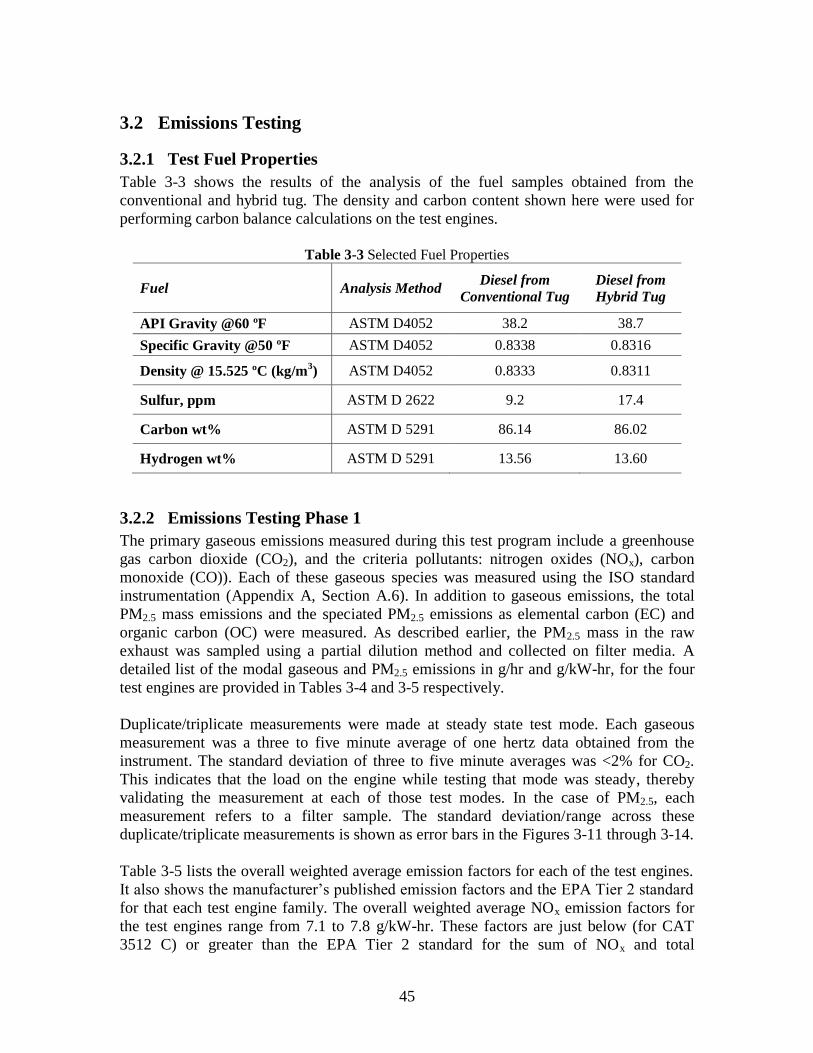
45

3.2 Emissions Testing

3.2.1 Test Fuel Properties

Table 3-3 shows the results of the analysis of the fuel samples obtained from the

conventional and hybrid tug. The density and carbon content shown here were used for

performing carbon balance calculations on the test engines.

Table 3-3 Selected Fuel Properties

Fuel Analysis Method Diesel from

Conventional Tug

Diesel from

Hybrid Tug

API Gravity @60 ºF ASTM D4052 38.2 38.7

Specific Gravity @50 ºF ASTM D4052 0.8338 0.8316

Density @ 15.525 ºC (kg/m3) ASTM D4052 0.8333 0.8311

Sulfur, ppm ASTM D 2622 9.2 17.4

Carbon wt% ASTM D 5291 86.14 86.02

Hydrogen wt% ASTM D 5291 13.56 13.60

3.2.2 Emissions Testing Phase 1

The primary gaseous emissions measured during this test program include a greenhouse

gas carbon dioxide (CO2), and the criteria pollutants: nitrogen oxides (NOx), carbon

monoxide (CO)). Each of these gaseous species was measured using the ISO standard

instrumentation (Appendix A, Section A.6). In addition to gaseous emissions, the total

PM2.5 mass emissions and the speciated PM2.5 emissions as elemental carbon (EC) and

organic carbon (OC) were measured. As described earlier, the PM2.5 mass in the raw

exhaust was sampled using a partial dilution method and collected on filter media. A

detailed list of the modal gaseous and PM2.5 emissions in g/hr and g/kW-hr, for the four

test engines are provided in Tables 3-4 and 3-5 respectively.

Duplicate/triplicate measurements were made at steady state test mode. Each gaseous

measurement was a three to five minute average of one hertz data obtained from the

instrument. The standard deviation of three to five minute averages was <2% for CO2.

This indicates that the load on the engine while testing that mode was steady, thereby

validating the measurement at each of those test modes. In the case of PM2.5, each

measurement refers to a filter sample. The standard deviation/range across these

duplicate/triplicate measurements is shown as error bars in the Figures 3-11 through 3-14.

Table 3-5 lists the overall weighted average emission factors for each of the test engines.

It also shows the manufacturer’s published emission factors and the EPA Tier 2 standard

for that each test engine family. The overall weighted average NOx emission factors for

the test engines range from 7.1 to 7.8 g/kW-hr. These factors are just below (for CAT

3512 C) or greater than the EPA Tier 2 standard for the sum of NOx and total

46

hydrocarbon (THC) emissions of 7.2 g/kW-hr. The weighted average PM2.5 emission

factors for the CAT 3512 C and Cummins engines, ranging from 0.053 to 0.097 g/kW-h,

are well below the EPA Tier 2 standard of 0.20 g/kW-hr. The JD 6081 auxiliary engine

however reported an overall weighted average PM2.5 emission factor of 0.24 g/kW-hr

which is greater than the emissions standard. The measured emissions factors for the

CAT 3512 C engine are comparable to the manufacturer’s published values. For the

Cummins engines, we find that the measured NOx emission factors are larger and PM2.5

emission factors smaller than the manufacturer’s numbers.

Table 3-4 Results for Phase 1 of Emissions Testing in g/hr

Target

Load

Actual

Load

NOx

(g/hr)

CO

(g/hr)

CO2

(kg/hr)

PM2.5

(g/hr)

EC

(g/hr)

OC

(g/hr)

Main Engine on Conventional Tug CAT 3512 C

Idle 7% 2439 136 98 6.3 1.7 5.3

25% 30% 4867 1324 402 94 3.9 108

50% 52% 7781 2774 681 195 90 105

75% 75% 9450 1015 1005 97 54 51

100% 100% 14124 1414 1325 173 101 100

Auxiliary Engine on Conventional Tug JD 6081

10% 11% 156 54 16 5.1 0.25 4.5

25% 26% 300 64 39 19.1 9.4 9.8

50% 40% 702 122 74 19.5 10.2 12.7

75% 71% 1224 251 106 28.0 7.2 19.2

Main Engine on Hybrid Tug Cummins QSK50-M

Idle 7% 1035 110 75 9.5 7.2 4.6

25% 26% 2674 318 262 9.8 6.2 6.9

50% 49% 5374 1054 541 50 36 22

75% 75% 7921 1608 799 58 39 29

100% 99% 10215 1236 1078 54 30 37

Auxiliary Engine on Hybrid Tug Cummins QSM11-M

25% 27% 600 66 65 9.8 6.6 4.1

50% 51% 1191 63 117 8.0 4.2 5.4

75% 73% 1729 69 173 9.1 4.9 6.4

47

Table 3-5 Emission Factors in g/kW-hr from Phase 1 of Testing

Target

Load

Actual

Load NOx CO CO2 PM2.5 EC OC

Main Engine on the Conventional Tug CAT 3512 C

Idle 7% 17.5 0.98 704 0.045 0.012 0.038

25% 30% 8.5 2.32 704 0.164 0.034 0.161

50% 52% 7.8 2.78 682 0.195 0.090 0.105

75% 75% 6.6 0.71 705 0.068 0.038 0.036

100% 100% 7.4 0.74 697 0.091 0.036 0.064

Wt. Avg. 7.1 1.1 701 0.097 0.047 0.059

Manf. Wt Avg. Nominal 6.31 0.49 657 0.10 n.a n.a

Manf. Wt Avg. NTE 7.57 0.89 n.a 0.12 n.a n.a

EPA Tier 2 Std 7.2* 5.0 n.a. 0.20 n.a n.a

Auxiliary Engine on the Conventional Tug JD 6081

10% 11% 5.9 1.28 771 0.38 0.19 0.19

25% 26% 7.3 1.27 774 0.20 0.11 0.13

50% 40% 8.9 1.83 773 0.20 0.05 0.14

75% 71% 7.3 2.52 746 0.24 0.01 0.21

Wt Avg 7.7 1.54 772 0.24 0.09 0.15

EPA Tier 2 Std 7.2* 5.0 n.a 0.20 n.a n.a

Main Engine on the Hybrid Tug Cummins QSK50-M

Idle 7% 11.0 1.2 792 0.101 0.077 0.049

25% 26% 7.7 0.9 756 0.028 0.018 0.020

50% 49% 8.2 1.6 823 0.075 0.055 0.033

75% 75% 7.9 1.6 799 0.058 0.039 0.029

100% 99% 7.7 0.9 812 0.041 0.022 0.028

Wt. Avg. n.a 7.8 1.4 798 0.053 0.034 0.026

Manf. Wt Avg. 6.53 0.81 n.a 0.09 n.a n.a


Auxiliary Engine on Hybrid Tug Cummins QSM11-M

25% 27% 7.0 0.8 765 0.116 0.078 0.048

50% 51% 7.4 0.4 725 0.050 0.026 0.034

75% 73% 7.5 0.3 749 0.039 0.021 0.028

Wt. Avg. 7.41 0.44 744 0.058 0.034 0.034

Manf. Wt Avg. 6.289 0.362 n.a 0.134 n.a n.a


Manf. Wt Avg. Manufacturer’s Weighted Average, NTE Not to Exceed

* Standard if for the sum of nitrogen oxides and total hydrocarbon emissions

48

Figure 3-11 Emission Factors for Main Engine on Conventional Tug CAT 3512C

Figure 3-12 Emission Factors for Auxiliary Engine on Conventional Tug JD 6081

0

5

10

15

20

25

Idle 25% 50% 75% 100% Wt Avg

Emis

sio

n F

acto

rs (

g/kW

-hr)

Engine Load

PM2.5*100 NOx CO*10 CO2/100PM2.5 *100 CO2 /100

0.0

2.0

4.0

6.0

8.0

10.0

11% 26% 49% 71% Wt Avg

Em

issi

on

Fa

cto

rs (

g/k

W-h

r)

Engine Load

PM2.5*10 NOx CO CO2/100PM2.5 *10 CO2 /100

49

Figure 3-13 Emission Factors for Main Engine on Hybrid Tug Cummins QSK50-M

Figure 3-14 Emission Factors for Auxiliary Engine on Hybrid Tug QSM11-M

0.0

3.0

6.0

9.0

12.0

15.0

18.0

21.0

24.0

Idle 26% 49% 75% 99% Wt Avg

Emis

sio

n F

acto

rs (

g/kW

-hr)

Engine Load

PM2.5*100 NOx CO*10 CO2/100PM2.5 *100 CO2 /100

0.0

2.0

4.0

6.0

8.0

10.0

12.0

14.0

27% 51% 73% Wt Avg

Emis

sio

n F

acto

rs (

g/kW

-hr)

Engine Load

PM2.5*100 NOx CO*10 CO2/100PM2.5 *100 CO2 /100

50

Diesel particulate matter primarily consists of elemental and organic carbon. Figure 3-15

shows a plot of the PM2.5 emissions in g/hr obtained from two separate methods –

gravimetric measurements of PM2.5 collected on Teflo®

filters and total carbon analysis

of PM2.5 collected on parallel Tissuquartz filters. These plots show that the total carbon

associated with PM2.5 is 3 to 19% greater than the total PM2.5 mass. This discrepancy can

be attributed to the positive organic artifact associated with the Tissuquartz filters.

Overall, PM2.5 measurements made by these two methods are in good agreement, thereby

increasing confidence in the measurement methods.

Figure 3-15 PM2.5 Mass Balance for A)Main Engine Conventional Tug CAT

3512 C B)Auxiliary Engine Conventional Tug JD 6081 C) Main Engine Hybrid

Tug Cummins QSK50-M D) Auxiliary Engine Hybrid Tug Cummins QSM11-M

y = 1.03x

R² = 0.93

0

7

14

21

28

35

0 10 20 30 40

To

tal C

arb

on

in

PM

Ma

ss (

g/h

r)

Gravimetric PM Mass(g/hr)

y = 1.18x

R² = -0.15

0

4

8

12

16

0 5 10 15

To

tal C

arb

on

in

PM

2.5

Ma

ss (

g/h

r)

Gravimetric PM2.5 Mass (g/hr)

y = 1.19x

R² = 0.96

0

20

40

60

80

100

0 50 100

To

tal C

arb

on

in

PM

2.5

Ma

ss (

g/h

r)

Gravimetric PM2.5 Mass (g/hr)

y = 1.08x

R² = 0.97

0

50

100

150

200

250

0 100 200 300

To

tal C

arb

on

in

PM

Ma

ss (

g/h

r)

Gravimetric PM Mass(g/hr)

A B

C D

51

3.2.3 Emissions Testing Phase 2

The goal of emissions testing Phase 2 was to determine an emissions profile of the test

engines across their whole operating range. As mentioned in Section 2.6.3 the auxiliary

engine on the conventional tug was not tested in Phase 2 as it operates only at the 12%

load point which was characterized during Phase 1. The other three engines were tested at

several steady state load points across their entire operating range including those from

Phase 1.

During this phase gaseous emissions of carbon dioxide, nitrogen oxides and carbon

monoxide were measured based on the ISO methods. Real-time PM2.5 mass

concentrations were measured using TSI’s DustTrak. One five minute measurement was

made at each test mode. This measurement is an average of one hertz data obtained from

the gas and PM analyzers for the entire sample time. The standard deviation in the CO2

measurement at each test mode was determined to be <2% indicating that the engine was

indeed at steady state during sampling. Test results are provided in Table 3-6.

Figures 3-16, 3-17 and 3-18 show a comparison of the engine load, gaseous emissions

and PM2.5 concentrations in the raw exhaust from Phases 1 and 2. For all three engines

the CO2 and NOx emissions from the two phases are found to be in good agreement. The

slightly higher CO2 emissions in Phase 2 can be attributed to the increase in the engine

load. The CO emissions for the two main engines obtained from the two phases were not

comparable. Therefore the CO emissions were not used in the final analysis.

Gravimetric PM2.5 measurements made in Phase 1 using Teflo® filters followed the ISO

reference methods. Measurements made in Phase 2 using TSI’s DustTrak give an

indication of the trends across engine loads but do not provide accurate numbers.

Therefore trend-lines showing variation in PM2.5 concentrations as a function of engine

load were plotted through the gravimetric filter measurements following the trends

obtained from real-time measurements in Phase 2. These trend-lines are shown in Figures

3-16 through 3-18. PM2.5 concentration (mg/m3) in the raw exhaust, for each test mode in

Phase 2, was calculated using these trend-lines. Finally the PM2.5 emissions in g/hr were

determined using these calculated concentrations and exhaust flows.

Figures 3-19, 3-20 and 3-21 show the variation in gaseous and PM2.5 mass emissions in

g/hr as a function of engine load. These emission profiles are used along with the engine

histograms to determining the total emissions from each engine at the different tug

operating modes.

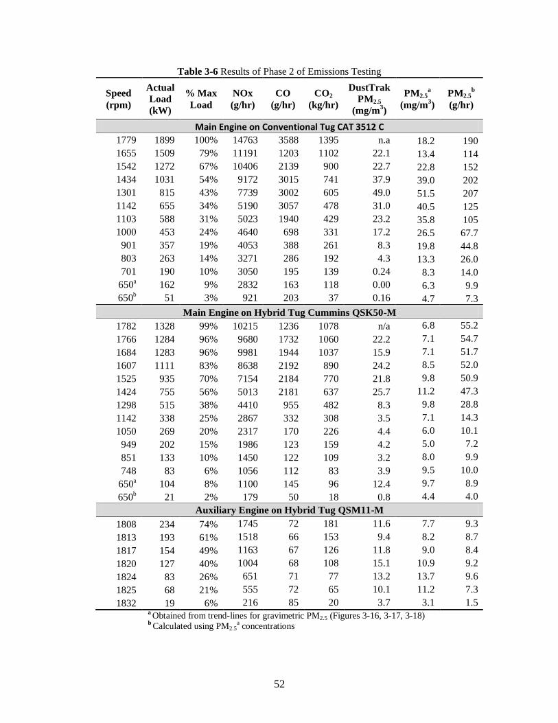
52

Table 3-6 Results of Phase 2 of Emissions Testing

Speed

(rpm)

Actual

Load

(kW)

% Max

Load

NOx

(g/hr)

CO

(g/hr)

CO2

(kg/hr)

DustTrak

PM2.5

(mg/m3)

PM2.5a

(mg/m3)

PM2.5b

(g/hr)

Main Engine on Conventional Tug CAT 3512 C

1779 1899 100% 14763 3588 1395 n.a 18.2 190

1655 1509 79% 11191 1203 1102 22.1 13.4 114

1542 1272 67% 10406 2139 900 22.7 22.8 152

1434 1031 54% 9172 3015 741 37.9 39.0 202

1301 815 43% 7739 3002 605 49.0 51.5 207

1142 655 34% 5190 3057 478 31.0 40.5 125

1103 588 31% 5023 1940 429 23.2 35.8 105

1000 453 24% 4640 698 331 17.2 26.5 67.7

901 357 19% 4053 388 261 8.3 19.8 44.8

803 263 14% 3271 286 192 4.3 13.3 26.0

701 190 10% 3050 195 139 0.24 8.3 14.0

650a 162 9% 2832 163 118 0.00 6.3 9.9

650b 51 3% 921 203 37 0.16 4.7 7.3

Main Engine on Hybrid Tug Cummins QSK50-M

1782 1328 99% 10215 1236 1078 n/a 6.8 55.2

1766 1284 96% 9680 1732 1060 22.2 7.1 54.7

1684 1283 96% 9981 1944 1037 15.9 7.1 51.7

1607 1111 83% 8638 2192 890 24.2 8.5 52.0

1525 935 70% 7154 2184 770 21.8 9.8 50.9

1424 755 56% 5013 2181 637 25.7 11.2 47.3

1298 515 38% 4410 955 482 8.3 9.8 28.8

1142 338 25% 2867 332 308 3.5 7.1 14.3

1050 269 20% 2317 170 226 4.4 6.0 10.1

949 202 15% 1986 123 159 4.2 5.0 7.2

851 133 10% 1450 122 109 3.2 8.0 9.9

748 83 6% 1056 112 83 3.9 9.5 10.0

650a 104 8% 1100 145 96 12.4 9.7 8.9

650b 21 2% 179 50 18 0.8 4.4 4.0

Auxiliary Engine on Hybrid Tug QSM11-M

1808 234 74% 1745 72 181 11.6 7.7 9.3

1813 193 61% 1518 66 153 9.4 8.2 8.7

1817 154 49% 1163 67 126 11.8 9.0 8.4

1820 127 40% 1004 68 108 15.1 10.9 9.2

1824 83 26% 651 71 77 13.2 13.7 9.6

1825 68 21% 555 72 65 10.1 11.2 7.3

1832 19 6% 216 85 20 3.7 3.1 1.5 a

Obtained from trend-lines for gravimetric PM2.5 (Figures 3-16, 3-17, 3-18) b

Calculated using PM2.5a concentrations

53

Figure 3-16 Comparison of Phases 1 & 2 for Main Engine on Conventional Tug CAT 3512 C

y = 1.08x

R² = 1.00

0

400

800

1200

1600

0 500 1000 1500

CO

2(k

g/h

r) -

Ph

ase

2

CO2 (kg/hr) - Phase 1

y = 1.50x

R² = 0.44

0

1000

2000

3000

4000

5000

0 1000 2000 3000

CO

(g

/hr)

-P

ha

se 2

CO (g/hr) - Phase 1

0

10

20

30

40

50

60

0 500 1000 1500 2000

PM

mg

/m^

3

Engine Load kW

DustTrak Phase 2 Gravimetric Filter Phase 1

y = 1.03x

R² = 0.99

0

500

1000

1500

2000

2500

0 1000 2000

En

gin

e L

oa

d (

kW

) -

Ph

ase

2

Engine Load (kW)- Phase 1

y = 1.10x

R² = 0.98

0

4000

8000

12000

16000

20000

0 5000 10000 15000

NO

x (

g/h

r) -

Ph

ase

2

NOx (g/hr) - Phase 1

54

Figure 3-17 Comparison of Phases 1 & 2 for Main Engine of Hybrid Tug Cummins QSK50-M

y = 1.05x

R² = 0.98

0

200

400

600

800

1000

1200

0 500 1000 1500

CO

2E

mis

sio

ns

-P

ha

se 2

(kg

/hr)

CO2 Emissions - Phase 1(kg/hr)

y = 1.51x

R² = 0.89

0

500

1000

1500

2000

2500

3000

0 500 1000 1500 2000

CO

E

mis

sio

ns

-P

ha

se 2

(g

/hr)

CO Emissions - Phase 1 (g/hr)

0.0

5.0

10.0

15.0

20.0

25.0

30.0

0 500 1000 1500

PM

(m

g/m

3)

Engine Load (kW)

Gravimetric PM - Phase 1 DustTrak PM - Phase 2

y = 1.04x

R² = 0.96

0

400

800

1200

1600

0 500 1000 1500

En

gin

e L

oa

d -

Ph

ase

2 (

kW

)

Engine Load - Phase 1 (kW)

y = 0.99x

R² = 0.98

0

2000

4000

6000

8000

10000

12000

0 10000 20000

NO

x E

mis

sio

ns

-P

ha

se 2

(g

/hr)

NOx Emissions - Phase 1 (g/hr)

55

Figure 3-18 Comparison of Phases 1 & 2 for Auxiliary

Engine on Hybrid Tug Cummins QSM11-M

y = 1.07x

R² = 0.99

0

40

80

120

160

200

0 50 100 150 200

CO

2E

mis

sio

ns

-P

ha

se 2

(kg

/hr)

CO2 Emissions - Phase 1 (kg/hr)

y = 1.06x

R² = 0.78

66

69

72

75

62 64 66 68 70

CO

Em

issi

on

s -

Ph

ase

2 (

g/h

r)

CO Emissions - Phase 1 (g/hr)

0.0

3.0

6.0

9.0

12.0

15.0

18.0

0 50 100 150 200 250

PM

(m

g/m

3)

Engine Load (kW)

Gravimetric PM - Phase 1 DustTrak PM - Phase 2

y = 0.99x

R² = 1.00

0

50

100

150

200

250

0 100 200 300

En

gin

e L

oa

d -

Ph

ase

2 (

kW

)

Engine Load - Phase 1 (kW)

y = 1.01x

R² = 0.99

0

400

800

1200

1600

2000

0 1000 2000

NO

x E

mis

sio

ns

-P

ha

se 2

(g

/hr)

NOx Emissions - Phase 1 (g/hr)

56

Figure 3-19 Emissions Profile for Main Engine on Conventional Tug CAT 3512 C

Figure 3-20 Emissions Profile of Main Engine on Hybrid Tug QSK50-M

0

50

100

150

200

250

0

2000

4000

6000

8000

10000

12000

14000

16000

0 500 1000 1500 2000

PM

Em

issi

on

s (g

/hr)

Ga

seo

us

Em

issi

on

(g

/hr)

Engine Load kW

NOx CO CO2/100 PMCO2/100

0

10

20

30

40

50

60

0

2000

4000

6000

8000

10000

12000

0 500 1000 1500

PM

Em

issi

on

s (g

/hr)

Gase

ou

s E

mis

sion

(g/h

r)

Engine Load kW


57

Figure 3-21 Emissions Profile of Auxiliary Engine on Hybrid Tug Cummins QSK11-M

3.2.4 Carbon Balance

As a part of the UCR’s QA/QC the mass balance between the carbon in the fuel and the

carbon measured in the exhaust is checked. For this project the fuel flow was not directly

measured, instead the instantaneous fuel flow rate in cubic centimeters per minute was

retrieved from the engine ECM. The carbon from the fuel in g/hr was calculated using

this fuel flow data along with the carbon content and density of fuel obtained from the

fuel sample analysis (Section 3.2.1). Approximately 99% of the carbon from the fuel is

converted to CO2. The amount of carbon in the exhaust was calculated from the measured

CO2 and CO emissions.

As mentioned in Section 2.6.6, we were unable to retrieve the inlet air and temperature

readings from ECM of the auxiliary engine on the conventional tug JD 6081. The exhaust

flow rate for this engine was estimated the instantaneous fuel flow data from its ECM.

Therefore a plot of the carbon from the fuel versus the carbon measured in the exhaust

will merely yield a 1-1 line. Hence, this engine is not included in this analysis.

Plots of the carbon in the fuel versus the carbon in the exhaust for the other three test

engines, obtained from both phases of emissions testing, are plotted in Figure 3-22. The

ECM data was found to be 13% to 16% lower than the measured carbon in the exhaust

for the main engines and 5% higher for the auxiliary engine on the hybrid. For most

diesel engines the correlation between fuel flow and carbon in the exhaust will be < 2%.

In this test, the fuel flow was not measured. The engine ECM provides an estimate of the

0.0

2.0

4.0

6.0

8.0

10.0

12.0

0

300

600

900

1200

1500

1800

2100

0 50 100 150 200 250

PM

Em

issi

on

s (g

/hr)

Ga

seo

us

Em

issi

on

(g

/hr)

Engine Load kW


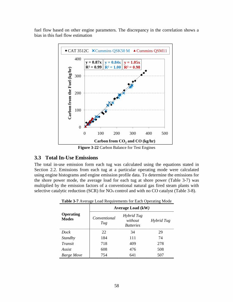
58

fuel flow based on other engine parameters. The discrepancy in the correlation shows a

bias in this fuel flow estimation

Figure 3-22 Carbon Balance for Test Engines

3.3 Total In-Use Emissions

The total in-use emission form each tug was calculated using the equations stated in

Section 2.2. Emissions from each tug at a particular operating mode were calculated

using engine histograms and engine emission profile data. To determine the emissions for

the shore power mode, the average load for each tug at shore power (Table 3-7) was

multiplied by the emission factors of a conventional natural gas fired steam plants with

selective catalytic reduction (SCR) for NOx control and with no CO catalyst (Table 3-8).

Table 3-7 Average Load Requirements for Each Operating Mode

Operating

Modes

Average Load (kW)

Conventional

Tug

Hybrid Tug

without

Batteries

Hybrid Tug

Dock 22 34 29

Standby 184 111 74

Transit 718 409 278

Assist 608 476 508

Barge Move 754 641 507

y = 0.87x

R² = 0.99

y = 0.84x

R² = 1.00

y = 1.05x

R² = 0.98

0

100

200

300

400

0 100 200 300 400 500

Ca

rbo

n f

rom

th

e F

uel

(k

g/h

r)

Carbon from CO2 and CO (kg/hr)

CAT 3512C Cummins QSK50 M Cummins QSM11

59

Table 3-8 Emission Factors for Shore Power17, 18

Emission Factor

lbs/106scf lbs/MW-hra g/kW-hr

PM2.5 7.6 0.087 29

NOx 10 0.117 74

CO2 120000 1371 278 a heating value of natural gas = 1,050 Btu/scf, power generation heat rate = 12,000 Btu/kW-hr

Table 3-9 lists the calculated emissions in g/hr of NOx, PM2.5 and CO2 at each operating

mode for the conventional tug, hybrid tug and hybrid tug without batteries. The table also

provides overall emissions from each tug calculated based on individual and average

weighing factors for each operating mode.

The reductions in overall PM2.5, NOx and CO2 emissions for the hybrid tug compared to

the conventional tug was found to be 73%, 51% and 27% respectively. The tug company

saw a fuel savings of about 25-28% while comparing conventional tug with the hybrid

over an eight month period. The CO2 reductions calculated from this study are in good

agreement with the fuel savings seen by the tug owner, thereby increasing confidence in

the test protocol and analysis technique.

The initial hypothesis for the emissions reduction was as follows: Conventional tug spend

considerable amount of time in the standby mode with one auxiliary engine and two main

engines idling. The hybrid tug switches between batteries and one auxiliary. So a

significant fraction of the emission savings would occur in this mode.

The final results show that the tugs spend only 7% of their total time in this mode. As a

result, its contribution to the overall emission reductions was found to be small ~4% for

PM2.5 and ~14% for NOx and CO2. The transit mode was found to be the largest

contributor to the overall emission reductions ~50% for PM2.5, ~53% for NOx, ~78% for

CO2. This is due to the significantly lower loads required to transit with the hybrid tug

versus the conventional tug (Table 3-7).

The emission reductions results for the hybrid tug operating without batteries show that

the bulk of the emission savings (97% for PM2.5, 95% for NOx, 70% for CO2) is a result

of the diesel electric drive train and not the batteries. The diesel electric drive train allows

auxiliary power to be used for propulsion. This reduces the total load requirement for the

transit and standby operations significantly thereby reducing the overall emissions from

the tug.

Since the conventional tug and the hybrid tug have engines from different engine

manufacturers with different power ratings a couple of retrofit scenarios were modeled.

Retrofit scenario 1: This scenario assumes that both tugs have the same set of engines.

For this purpose the main and auxiliary engine with the higher power ratings, CAT 3512

C main engines and Cummins QSK11-M auxiliary engines, were chosen. The emission

profiles of the chosen engines were coupled with the engines histograms for each tug to

60

determine the total emissions at each operating mode (Table 3-10). These were then

multiplied by the individual and average weighting factors to determine the overall in-use

emissions for this scenario. The reductions in the overall in-use emissions calculated

based on average weighting factors was found to be 58%, 39%, 32% for PM2.5, NOx and

CO2 respectively. The reductions in PM2.5 and CO2 increased while that of NOx

decreased in this scenario when compared to the actual numbers. Again we find that the

bulk of the reductions occur in the transit mode. Also most of the reductions are a result

of the energy management system rather than the batteries.

Retrofit Scenario 2: Conventional tugs typically have auxiliary engines with a lower

power rating like the JD 6081. Therefore, a more realistic retrofit scenario would be:

Conventional tug powered by CAT 3512 C main engines and the JD 6081 auxiliaries;

Hybrid tug powered by CAT 3512 C main engines and the Cummins QSK11-M

auxiliaries. Results for this retrofit scenario 2 are provided in Table 3-11. The reduction

in the overall in-use emissions seen in Retrofit Scenario 2 was found to be similar to that

of Retrofit Scenario 1.

61

Table 3-9 Modal and Overall Emission Reductions with Hybrid Technology

Operating Mode

Operating Mode

Weighting Factors PM2.5 (g/hr) NOx (g/hr) CO2 (kg/hr)

Con. Hyb. Average Con. Hyb_NB Hyb. Con. Hyb_NB Hyb. Con. Hyb_NB Hyb.

Shore Power 0.01 0.18 0.00 0.0009 0.0013 0.0012 0.0011 0.0017 0.0015 0.014 0.021 0.018

Dock 0.53 0.35 0.54 5.1 3.2 1.1 156 309 89 16 33 10

Standby 0.07 0.07 0.07 26.6 8.7 7.3 3757 832 677 176 83 68

Transit 0.16 0.18 0.17 114.8 16.9 15.5 7633 2683 2371 530 276 240

Barge Move 0.05 0.05 0.05 133.1 42.1 36.4 7666 5588 4659 555 569 457

Ship Assist 0.17 0.17 0.17 82.0 36.4 38.3 6452 4270 4541 424 423 450

Overall Emissions Using Individual Wt. Factors 44.1 13.2 12.1 3088 1676 1528 208 169 153

% Reduction compared to Conventional Tug

70% 73%

46% 51%

19% 27%

Overall Emissions using Average Wt. Factors 45.2 13.6 12.2 3153 1708 1523 213 173 152


70% 73%

46% 52%

19% 29%

Wt. Factors- Weighting Factors, Con.-Conventional Tug, Hyb.-Hybrid Tug, Hyb_NB-Hybrid Tug without Batteries

Figure 3-23 Overall Emission Reductions

70%

46%

19%

73%

51%

27%

70%

46%

19%

73%

52%

29%

0%

30%

60%

90%

PM NOx CO2

% R

ed

uct

ion

in T

ota

l In

-Use

Em

issi

on

s

Individual Weighing Factors for Hybrid without Batteries

Individual Weighing Factors for Hybrid

Average Weighing Factors for Hybrid without Batteries

Average Weighing Factors for Hybrid

CO2

62

Table 3-10 Modal and Overall Emissions Reductions with Hybrid Technology for Retrofit Scenario 1 Assumption: Both tugs have CAT 3512 C main engines and Cummins QSK11-M auxiliaries

Operating Mode

Operating Mode


Con. Hyb. Average Con. Hyb_NB .Hyb Con. Hyb_NB Hyb. Con. Hyb_NB Hyb.

Shore Power 0.01 0.18 0 0.0009 0.0013 0.0012 0.0011 0.0017 0.0015 0.014 0.021 0.018

Dock 0.53 0.35 0.54 1.9 3.2 1.1 241 309 89 18 33 10

Standby 0.07 0.07 0.07 23.5 8.7 7.1 3842 1127 886 178 84 69

Transit 0.16 0.18 0.17 111.6 24.4 19.0 7718 3021 2679 531 270 235

Barge Move 0.05 0.05 0.05 130.0 75.7 55.3 7751 7289 6421 557 534 435

Ship Assist 0.17 0.17 0.17 78.8 59.8 60.4 6537 5934 6197 426 394 422



50% 57%

33% 38%

23% 31%



51% 58%

33% 39%

23% 32%


Figure 3-24 Overall Emission Reductions for Retrofit Scenario 1

50%

33%23%

57%

38%31%

51%

33%23%

58%

39%32%

0%

20%

40%

60%

80%

PM NOx CO2

% R

ed

uct

ion

in T

ota

l In

-U

se E

mis

sio

ns




Average Weighing Factors for HybridCO2

63

Table 3-11 Modal and Overall Emissions Reductions with Hybrid Technology for Retrofit Scenario 2 Assumption: Conventional tug has CAT 3512C mains and JD 6081 auxiliaries; hybrid tug has CAT 3512 C mains and Cummins QSK11-M auxiliaries

Operating Mode

Operating Mode


Con. Hyb. Average Con. Hyb_NB Hyb. Con. Hyb_NB Hyb. Con. Hyb_NB Hyb.

Shore Power 0.01 0.18 0 0.0009 0.0013 0.0012 0.0011 0.0017 0.0015 0.014 0.021 0.018

Dock 0.53 0.35 0.54 5.1 3.2 1.1 156 309 89 16.0 32.8 9.9

Standby 0.07 0.07 0.07 27 9 7 3757 1127 886 176 84 69

Transit 0.16 0.18 0.17 115 24 19 7633 3021 2679 530 270 235

Barge Move 0.05 0.05 0.05 133 76 55 7666 7289 6421 555 534 435

Ship Assist 0.17 0.17 0.17 82 60 60 6452 5934 6197 424 394 422



54% 60%

31% 36%

22% 30%



54% 61%

31% 38%

23% 32%


Figure 3-25 Overall Emission Reductions for Retrofit Scenario 2

54%

31%22%

60%

36%30%

54%

31%23%

61%

38%32%

0%

20%

40%

60%

80%

PM NOx CO2

% R

ed

uct

ion

in T

ota

l In

-U

se E

mis

sio

ns




Average Weighing Factors for Hybrid

CO2

64

4 Summary and Recommendations The primary goal of this project was to develop and implement a test protocol to

determine the emission benefits of a hybrid tug. For this purpose, a conventional and a

hybrid tug built on the same classification were chosen. The conventional tug was

powered by four diesel engines while the hybrid tug operated on four diesel engines and

126 batteries. All diesel engines were EPA Tier 2 certified.

The first step of the research involved the development of a data logging system capable

of continuously logging the daily activity of all the power sources on each tug. This

system was used to collect one month of activity data from each tug. Gigabytes of data

were analyzed to establish weighing factor for different tug operating modes and develop

engine histograms at each operating mode for all the eight engines.

The second step of the research was the implementation of a two phase emissions testing

program to establish the emissions profile of the diesel engines across their entire

operating range. Gaseous and PM2.5 emissions were measured as per the ISO 8178-1

protocols. Several quality control checks such as fuel carbon to exhaust carbon balance,

total PM2.5 to speciated PM2.5 mass balance, <2% standard deviation in CO2 emission

factors at each of the steady state test mode, comparison with manufacturer’s reported

numbers and reasonable error bars on the final readings showing good repeatability and

reproducibility helped validate the emissions testing.

The final analysis combined engine histogram and emission profile data to determine in-

use emissions at each tug operating mode for both conventional and the hybrid tug. These

figures were coupled with the weighing factors for the operating modes to get the overall

in-use emissions in g/hr for each tug. Significant emission benefits were observed for the

hybrid technology. The reductions in the fuel equivalent CO2 emissions were in good

agreement with the fuel savings measured by the tugboat owner over an eight month

period. This quality check increases the confidence in the test protocol and analysis

techniques.

The major findings of this program include:

Tug boats involved in this study operate in five different modes – dock, standby,

transit, ship assist and barge moves. The average weighing factors for these

operating modes were found to be 0.54, 0.07, 0.17, 0.17 and 0.05 respectively.

The conventional tug tested in this program did not plug into shore power while

the hybrid tug spent one-third of the time at dock plugged in.

The average loads on the main and auxiliary engines of the conventional tug are

16% and 12% of the maximum load. For the hybrid tug average loads of main and

auxiliary engines were found to be 12% and 34% of the rated power. These

average operating loads are well below the load factors of the standard ISO duty

cycles. This finding highlights the importance of developing of in-use duty cycles

65

that help predict the emissions at source more accurately thereby reducing the

uncertainties in emission inventories.

Four EPA Tier 2 certified in-use marine engines were tested following the load

points in the standard ISO cycles. The overall weighted average NOx emission

factors for these engines range from 7.1 to 7.8 g/kW-hr. These factors are just

below (for CAT 3512 C) or greater than the EPA Tier 2 standard for the sum of

NOx and total hydrocarbon (THC) emissions of 7.2 g/kW-hr. The weighted

average PM2.5 emission factors, for three out of the four engines, were well below

the EPA Tier 2 standard of 0.20 g/kW-hr.

Overall in-use emission reductions with the hybrid technology were found to be

73% for PM2.5, 51% for NOx and 27% for CO2.

The diesel electric drive train on the hybrid tug that allows the use of auxiliary

power for propulsion was the primary cause for the overall in-use emission

reductions as opposed to the energy storage device (batteries).

The transit operating mode was the most significant contributor to the overall

emission reductions. In this mode the hybrid tug was powered by one or two

auxiliary engines and batteries while the conventional tug used one auxiliary and

two main engines.

Recommendations for further studies

The hybrid tug can also be operated as a plug in hybrid. During this test program

the tug could not be operated as a plug in hybrid due to lack of sufficient shore

power. Future studies on the hybrid tug should involve tailoring the existing test

protocol to determine the emission benefits of the plug in hybrid.

Activity data from the hybrid tug operating without batteries was collected for a

period of only 1.5 days. This data revealed that the primary cause of emission

benefits of the hybrid tug was the diesel electric drive train and not the batteries.

To increase the confidence in this conclusion activity data on the hybrid tug

operating without batteries should be collected for a larger time period of

approximately one month.

66

References 1. Corbett, J. J.; Winebrake, J. J.; Green, E. H.; Kasibhatla, P.; Eyring, V.; Lauer, A.,

Mortality from ship emissions: A global assessment. Environmental Science &

Technology 2007, 41, (24), 8512-8518.

2. Deniz, C.; Durmusoglu, Y., Estimating shipping emissions in the region of the

Sea of Marmara, Turkey. Science of the Total Environment 2008, 390, (1), 255-

261.

3. Lucialli, P.; Ugolini, P.; Pollini, E., Harbour of Ravenna: The contribution of

harbour traffic to air quality. Atmospheric Environment 2007, 41, (30), 6421-

6431.

4. Saxe, H.; Larsen, T., Air pollution from ships in three Danish ports. Atmospheric

Environment 2004, 38, (24), 4057-4067.

5. Schrooten, L.; De Vlleger, I.; Panis, L. I.; Styns, K.; Torfs, R., Inventory and

forecasting of maritime emissions in the Belgian sea territory, an activity-based

emission model. Atmospheric Environment 2008, 42, (4), 667-676.

6. Vutukuru, S.; Dabdub, D., Modeling the effects of ship emissions on coastal air

quality: A case study of southern California. Atmospheric Environment 2008, 42,

(16), 3751-3764.

7. Starcrest Consulting LLC, Port of Long Beach Air Emissions Inventory - 2005.

2007, Prepared for the Port of Long Beach.

8. Starcrest Consulting LLC, Port of Los Angeles Inventory of Air Emissions. 2009,

Prepared for the Port of Los Angeles.

9. Corbett, J. J.; Fischbeck, P. S., Emissions from Waterborne Commerce Vessels in

United States Continental and Inland Waterways. Environmental Science &

Technology 2000, 34, (15), 3254-3260.

10. Corbett, J. J.; Robinson, A. L., Measurements of NOx Emissions and In-Service

Duty Cycle from a Towboat Operating on the Inland River System.

Environmental Science & Technology 2001, 35, (7), 1343-1349.

11. U.S. Environmental Protection Agency, Final Rule: Control of Emissions of Air

Pollution from Locomotives and Marine Compression-Ignition Engines Less

Than 30 Liters per Cylinder. 2008, 40 CFR, Parts 85-94.

12. Cooper, D. A., Exhaust emissions from high speed passenger ferries. Atmospheric

Environment 2001, 35, (24), 4189-4200.

13. Cooper, D. A.; Peterson, K.; Simpson, D., Hydrocarbon, PAH and PCB emissions

from ferries: A case study in the Skagerak-Kattegatt-Öresund region. Atmospheric

Environment 1996, 30, (14), 2463-2473.

14. Society of Automotive Engineers, Recommended Practices for Measuring

Exhaust Emissions and Fuel Economy of Hybrid Electric Vehicles. 1999, SAE

J1711.

15. California Air Resources Board, California Exhaust Emission Standards and Test

Procedures for 2009 and Subsequent Model Zero-Emission Vehicles, and Hybrid

Electric Vehicles, In the Passenger Car, Light-Duty Truck and Medium-Duty

Vehicle Classes. 2009.

16. International Organization for Standardization, ISO 8178-1 Reciprocating internal

combustion engines - Exhaust emission measurement - Part 1: Test-bed

67

measurement of gaseous and particulate exhaust emissions. 1996, First Edition

1996-08-15.

17. Environ International Corporation, Cold Ironing Cost Effectiveness Study. 2004,

Prepared for Port of Long Beach.

18. U.S. Environmental Protection Agency, AP-42 Compilation of Air Pollutant

Emission Factors. 2004, Fifth Edition Vol I.

1

Appendix A - Measuring Gaseous & Particulate Emissions

A-

2

A.1 Scope ISO 8178-1

1 and ISO 8178-2

2, when combined with engine load and speed duty cycles

provided in IS0 8178-4, specify the measurement and evaluation methods for gaseous

and particulate exhaust emissions. The emission results represent the mass rate of

emissions per unit of work accomplished. Specific emission factors are based on brake

power measured at the crankshaft, the engine being equipped only with the standard

auxiliaries necessary for its operation. Per ISO, auxiliary losses are <5% of the maximum

observed power.

IMO ship pollution rules and measurement methods are contained in the “International

Convention on the Prevention of Pollution from Ships”, known as MARPOL 73/783, and

sets limits on NOx and SOx emissions from ship exhausts. The intent of this protocol was

to conform as closely as practical to both the ISO and IMO standards.

A.2 Sampling System for Measuring Gaseous and Particulate

Emissions A properly designed sampling system is essential for accurate collection of a

representative sample from the exhaust and subsequent analysis. ISO points out that

particulate must be collected in either a full flow or partial flow dilution system and UCR

chose the partial flow dilution system with single venturi as shown in Figure A-1.

A partial flow dilution system was selected based on cost and the impossibility of a full

flow dilution for “medium and large” engine testing on the test bed and at site. The flow

in the dilution system eliminates water condensation in the dilution and sampling systems

and maintains the temperature of the diluted exhaust gas at <52°C before the filters. ISO

cautions the advantages of partial flow dilution systems can be lost to potential problems

such as: losing particulates in the transfer tube, failing to take a representative sample

from the engine exhaust and inaccurately determining the dilution ratio.

An overview of UCR’s partial dilution system shows that raw exhaust gas is transferred

from the exhaust pipe (EP) through a sampling probe (SP) and the transfer tube (TT) to a

dilution tunnel (DT) due to the negative pressure created by the venturi (VN) in DT. The

gas flow rate through TT depends on the momentum exchange at the venturi zone and is

therefore affected by the absolute temperature of the gas at the exit of TT. Consequently,

the exhaust split for a given tunnel flow rate is not constant, and the dilution ratio at low

load is slightly lower than at high load. More detail on the key components is provided in

Table A-1.

1 International Standards Organization, IS0 8178-1, Reciprocating internal combustion engines - Exhaust

emission measurement -Part 1: Test-bed measurement of gaseous particulate exhaust emissions, First

edition 1996-08-l5 2 International Standards Organization, IS0 8178-2, Reciprocating internal combustion engines - Exhaust

emission measurement -Part 2: Measurement of gaseous and particulate exhaust emissions at site, First

edition 1996-08-l5 3 International Maritime Organization, Annex VI of MARPOL 73/78 “Regulations for the Prevention of Air

Pollution from Ships and NOx Technical Code”.

A-

3

Figure A-1 Partial Flow Dilution System with Single Venturi,

Concentration Measurement and Fractional Sampling

A.3 Dilution Air System A partial flow dilution system requires dilution air and UCR uses compressed air in the

field as it is readily available. ISO recommends the dilution air be at 25±5°C, filtered and

charcoal scrubbed to eliminate background hydrocarbons. The dilution air may be

dehumidified. To ensure the compressed air is of a high quality UCR processes any

supplied air through a field processing unit that reduces the pressure to about 30psig as

that level allows a dilution ratio of about 5/1 in the geometry of our system. The next

stages, in sequence, include: a liquid knock-out vessel, desiccant to remove moisture with

silica gel containing an indicator, hydrocarbon removal with activated charcoal and a

HEPA filter for the fine aerosols that might be present in the supply air. The silica gel and

activated carbon are changed for each field campaign. Figure A-2 shows the field

processing unit in its transport case. In the field the case is used as a framework for

supporting the unit

Figure A-2 Field Processing Unit for Purifying Dilution Air in Carrying Case

A-

4

Table A-1 Components of a Sampling System: ISO/IMO Criteria & UCR Design

Section Selected ISO and IMO Criteria UCR Design

Exhaust

Pipe (EP)

In the sampling section, the gas velocity is > 10 m/s, except at idle, and bends are

minimized to reduce inertial deposition of PM. Sample position is 6 pipe

diameters of straight pipe upstream and 3 pipe diameters downstream of the

probe.

UCR follows the ISO

recommendation, as closely

as practical.

Sampling

Probe (SP)

The minimum inside diameter is 4 mm and the probe is an open tube facing

upstream on the exhaust pipe centerline. No IMO code.

UCR uses a stainless steel

tube with diameter of 8mm

placed near the center line.

Transfer

Tube (TT)

As short as possible and < 5 m in length;

Equal to/greater than probe diameter & < 25 mm diameter;

TTs insulated. For TTs > 1m, heat wall temperature to a minimum of 250°C or set for < 5% thermophoretic losses of PM.

UCR no longer uses a

transfer tube.

Dilution

Tunnel (DT)

shall be of a sufficient length to cause complete mixing of the exhaust and dilution air under turbulent flow conditions;

shall be at least 75 mm inside diameter (ID) for the fractional sampling type, constructed of stainless steel with a thickness of > 1.5 mm.

UCR uses fractional

sampling; stainless steel

tunnel has an ID of 50mm

and thickness of 1.5mm.

Venturi

(VN)

The pressure drop across the venturi in the DT creates suction at the exit of the

transfer tube TT and gas flow rate through TT is basically proportional to the

flow rate of the dilution air and pressure drop.

Venturi proprietary design

provided by MAN B&W;

provides turbulent mixing.

Exhaust Gas

Analyzers

(EGA)

One or several analyzers may be used to determine the concentrations.

Calibration and accuracy for the analyzers are like those for measuring the

gaseous emissions.

UCR uses a 5-gas analyzer

meeting IMO/ISO specs

A-

5

A.4 Calculating the Dilution Ratio According to ISO 8178, “it is essential that the dilution ratio be determined very

accurately” for a partial flow dilution system such as what UCR uses. The dilution ratio is

simply calculated from measured gas concentrations of CO2 and/or NOx in the raw

exhaust gas, the diluted exhaust gas and the dilution air. UCR has found it useful to

independently determine the dilution ration from both CO2 and NOx and compare the

values to ensure that they are within ±10%. UCR’s experience indicates the

independently determined dilution ratios are usually within 5%. At systematic deviations

within this range, the measured dilution ratio can be corrected, using the calculated

dilution ratio. According to ISO, dilution air is set to obtain a maximum filter face

temperature of <52°C and the dilution ratio shall be > 4.

A.5 Dilution System Integrity Check ISO describes the necessity of measuring all flows accurately with traceable methods and

provides a path and metric to quantifying the leakage in the analyzer circuits. UCR has

adopted the leakage test and its metrics as a check for the dilution system. According to

ISO the maximum allowable leakage rate on the vacuum side shall be 0.5% of the in-use

flow rate for the portion of the system being checked. Such a low leakage rate allows

confidence in the integrity of the partial flow system and its dilution tunnel. Experience

has taught UCR that the flow rate selected should be the lowest rate in the system under

test.

A.6 Measuring the Gaseous Emissions: CO, CO2, HC, NOx, O2,

SO2 Measurement of the concentration of the main gaseous constituents is one of the key

activities in measuring emission factors. This section covers the ISO/IMO protocols and

that used by UCR. For SO2, ISO recommends and UCR concurs that the concentration of

SO2 is calculated based on the fact that >95% of the fuel sulfur is converted to SO2.

A.6.1 Measuring Gaseous Emissions: ISO & IMO Criteria ISO specifies that either one or two sampling probes located in close proximity in the raw

gas can be used and the sample split for different analyzers. However, in no case can

condensation of exhaust components, including water and sulfuric acid, occur at any

point of the analytical system. ISO specifies the analytical instruments for determining

the gaseous concentration in either raw or diluted exhaust gases.

Heated flame ionization detector (HFID) for the measurement of hydrocarbons;

Non-dispersive infrared analyzer (NDIR) for the measurement of carbon monoxide and carbon dioxide;

Heated chemiluminescent detector (HCLD) or equivalent for measurement of nitrogen oxides;

Paramagnetic detector (PMD) or equivalent for measurement of oxygen.

ISO states the range of the analyzers shall accurately cover the anticipated concentration

of the gases and recorded values between 15% and 100% of full scale. A calibration

curve with five points is specified. However, with modern electronic recording devices,

A-

6

like a computer, ISO allows the range to be expanded with additional calibrations. ISO

details instructions for establishing a calibration curve below 15%. In general, calibration

curves must be < ±2% of each calibration point and by < ±1% of full scale zero.

ISO outlines their verification method. Each operating range is checked prior to analysis

by using a zero gas and a span gas whose nominal value is more than 80% of full scale of

the measuring range. If, for the two points considered, the value found does not differ by

more than ±4% of full scale from the declared reference value, the adjustment parameters

may be modified. If >4%, a new calibration curve is needed.

ISO & IMO specify the operation of the HCLD. The efficiency of the converter used for

the conversion of NO2 into NO is tested prior to each calibration of the NOx analyzer.

The efficiency of the converter shall be > 90%, and >95% is strongly recommended.

ISO requires measurement of the effects from exhaust gases on the measured values of

CO, CO2, NOx, and O2. Interference can either be positive or negative. Positive

interference occurs in NDIR and PMD instruments where the interfering gas gives rise to

the same effect as the gas being measured, but to a lesser degree. Negative interference

occurs in NDIR instruments due to the interfering gas broadening the absorption band of

the measured gas, and in HCLD instruments due to the interfering gas quenching the

radiation. Interference checks are recommended prior to an analyzer’s initial use and after

major service intervals.

A.6.2 Measuring Gaseous Emissions: UCR Design The concentrations of CO, CO2, NOx and O2 in the raw exhaust and in the dilution tunnel

are measured with a Horiba PG-250 portable multi-gas analyzer. The PG-250

simultaneously measures five separate gas components with methods recommended by

the ISO/IMO and U.S. EPA. The signal output of the instrument is connected to a laptop

computer through an RS-232 interface to continuously record measured values. Major

features include a built-in sample conditioning system with sample pump, filters, and a

thermoelectric cooler. The performance of the PG-250 was tested and verified under the

U.S. EPA ETV program.

Figure A-3 Setup Showing Gas Analyzer with Computer for Continuous Data Logging

A-

7

Details of the gases and the ranges for the Horiba instrument are shown in Table A-2.

Note that the Horiba instrument measures sulfur oxides (SO2); however, the UCR follows

the protocol in ISO and calculates the SO2 level from the sulfur content of the fuel as the

direct measurement for SO2 is less precise than calculation.

Table A-2 Detector Method and Concentration Ranges for Monitor

Component Detector Ranges

Nitrogen Oxides (NOx) Heated Chemiluminescence

Detector (HCLD)

0-25, 50, 100, 250, 500, 1000, &

2500 ppmv

Carbon Monoxide (CO) Non dispersive Infrared

Absorption (NDIR)

0-200, 500, 1000, 2000, & 5000

ppmv

Carbon Dioxide (CO2) Non dispersive Infrared

Absorption (NDIR) 0-5, 10, & 20 vol%

Sulfur Dioxide (SO2) Non dispersive Infrared

Absorption (NDIR) 0-200, 500, 1000, & 3000 ppmv

Oxygen Zirconium oxide sensor 0-5, 10, & 25 vol%

For quality control, UCR carries out analyzer checks with calibration gases both before

and after each test to check for drift. Because the instrument measures the concentration

of five gases, the calibration gases are a blend of several gases (super-blend) made to

within 1% specifications. Experience has shown that the drift is within manufacturer

specifications of ±1% full scale per day shown in Table A-3. The PG-250 meets the

analyzer specifications in ISO 8178-1 Section 7.4 for repeatability, accuracy, noise, span

drift, zero drift and gas drying.

Table A-3 Quality Specifications for the Horiba PG-250

Repeatability ±0.5% F.S. (NOx: </= 100ppm range CO: </= 1,000ppm range)

±1.0% F. S.

Linearity ±2.0% F.S.

Drift ±1.0% F. S./day (SO2: ±2.0% F.S./day)

A-

8

A.7 Measuring the Particulate Matter (PM) Emissions ISO 8178-1 defines particulates as any material collected on a specified filter medium

after diluting exhaust gases with clean, filtered air at a temperature of ≤52ºC, as measured

at a point immediately upstream of the primary filter. The particulate consists of

primarily carbon, condensed hydrocarbons and sulfates, and associated water. Measuring

particulates requires a dilution system and UCR selected a partial flow dilution system.

The dilution system design completely eliminates water condensation in the

dilution/sampling systems and maintains the temperature of the diluted exhaust gas at

≤52°C immediately upstream of the filter holders. IMO does not offer a protocol for

measuring PM. A comparison of the ISO and UCR practices for sampling PM is shown

in Table A-4.

Table A-4 Measuring Particulate by ISO and UCR Methods

ISO UCR

Dilution tunnel Either full or partial flow Partial flow

Tunnel & sampling system Electrically conductive Same

Pretreatment None Cyclone, removes >2.5µm

Filter material Fluorocarbon based Teflon (TFE)

Filter size, mm 47 (37mm stain diameter) Same

Number of filters in series Two One

Number of filters in parallel Only single filter Two; 1 Teflo® & 1 Tissuauartz

Number of filters per mode Single or multiple Multiple

Filter face temp. °C < 52 Same

Filter face velocity, cm/sec 35 to 80. ~33

Pressure drop, kPa For test <25 Same

Filter loading, µg >500 500-1,000 + water w/sulfate

Weighing chamber 22±3°C & RH= 45%± 8 Same

Analytical balance, LDL µg 10 0.5

Flow measurement Traceable method Same

Flow calibration, months < 3months Every campaign

Sulfur content: According to ISO, particulates measured using IS0 8178 are

“conclusively proven” to be effective for fuel sulfur levels up to 0.8%. UCR is often

faced with measuring PM for fuels with sulfur content exceeding 0.8% and has extended

this method to those fuels as no other method is prescribed for fuels with a higher sulfur

content.

A.7.1 Added Comments about UCR’s Measurement of PM In the field UCR uses a raw particulate sampling probe fitted close to and upstream of the

raw gaseous sample probe and directs the PM sample to the dilution tunnel. There are

two gases stream leaving the dilution tunnel; the major flow vented outside the tunnel and

the minor flow directed to a cyclone separator, sized to remove particles >2.5um. The

line leaving the cyclone separator is split into two lines; each line has a 47 Gelman filter

holder. One holder collects PM on a Teflo® filter and the other collects PM on a

Tissuquartz filter. UCR simultaneously collects PM on Teflo® and Tissuquartz filters at

each operating mode and analyzes them according to standard procedures.

A-

9

Briefly, PM mass collected on the Pall Gelman (Ann Arbor, MI) 47 mm Teflo® filters

was determined by the difference in weight of the filter before and after sample

collection. These filters were conditioned for 24 hours in an environmentally controlled

room (RH = 40%, T= 25°C) and weighed daily, using a Mettler Toledo UMX2

microbalance, until two consecutive weight measurements were within 3µg or 2%.

The 47mm 2500 QAT-UP Tissuquartz filters (Pall, Ann Arbor, MI) were preconditioned

for 5 hours at 600°C and stored at temperatures <4°C before and after sampling and

analysis. EC/OC analysis on the Tissuquartz filters was performed according to the

NIOSH method1 using Sunset Laboratories Thermal/Optical Carbon Aerosol Analyzer.

It is important to note that the simultaneous collection of PM on Tissuquartz and Teflo®

filters provides a comparative check of PM mass measured by two independent methods

and serves as an important quality check for measuring PM mass.

A.8 Measuring Real-Time Particulate Matter (PM) Emissions-

DustTrak In addition to the filter-based PM mass measurements, UCR takes continuous readings

with a Nephelometer (TSI DustTrak 8520) so as to capture both the steady-state and

transient data. The Dust Trak is a portable, battery-operated laser photometer that gives

real-time digital readout with the added benefits of a built-in data logger. The DustTrak

nephelometer is fairly simple to use and has

excellent sensitivity to untreated diesel exhaust. It

measures light scattered by aerosol introduced

into a sample chamber and displays the measured

mass density as units of mg/m3. As scattering per

unit mass is a strong function of particle size and

refractive index of the particle size distributions

and as refractive indices in diesel exhaust strongly

depend on the particular engine and operating

condition, some scientists question the accuracy

of these PM mass measurements. However, UCR

always references the DustTrak results to filter

based measurements and this approach has shown

that mass scattering efficiencies for both on-road

diesel exhaust and ambient fine particles have

values around 3m2/g. For these projects, a TSI

DustTrak 8520 nephelometer measuring 90light scattering at 780nm (near-infrared) is used.

Figure A-4 Picture of TSI DustTrak

1 NIOSH Manual of Analytical Methods National Institute of Occupational Safety and Health, Cincinnati,

OH; 1996.

A-

10

A.9 Quality Control/Quality Assurance (QC/QA) Each of the laboratory methods for PM mass and chemical analysis has a standard

operating procedure including the frequency of running standards and the repeatability

that is expected with a standard run. Additionally the data for the standards are plotted to

ensure that the values fall within the upper and lower control limits for the method and

that there is no obvious trends or bias in the results for the reference materials. As an

additional quality check, results from independent methods are compared and values

from this work are compared with previously published values, like the manufacturer

data base.

For the ISO cycles, run the engine at rated speed and the highest power possible

to warm the engine and stabilize emissions for about 30 minutes.

Determine a plot or map of the peak power at each engine speed (rpm), starting with rated speed. If UCR suspects the 100% load point at rated speed is

unattainable, then we select the highest possible load on the engine as Mode 1.

Emissions are measured while the engine operates according to the requirements of ISO-8178-E3 or ISO-8178-D2 cycles. For a diesel engine the highest power

mode is run first and then each mode was run in sequence The minimum time for

samples is 5 minutes and if necessary, the time was extended to collect sufficient

particulate sample mass or to achieve stabilization with large engines.

The gaseous exhaust emission concentration values are measured and recorded for

the last 3 min of the mode.

Engine speed, displacement, boost pressure, and intake manifold temperature are measured in order to calculate the gaseous flow rate.

Emissions factors are calculated in terms of grams per kilowatt hour for each of the operating modes and fuels tested, allowing for emissions comparisons of each

blend relative to the baseline fuel.

A-

1

Appendix B - Test Cycles and Fuels for

Different Engine Applications

B-

2

B.1 Introduction

Engines for off-road use are made in a much wider range of power output and used in a

more applications than engines for on-road use. The objective of IS0 8178-41 is provide

the minimum number of test cycles by grouping applications with similar engine

operating characteristics. ISO 8178-4 specifies the test cycles while measuring the

gaseous and particulate exhaust emissions from reciprocating internal combustion

engines coupled to a dynamometer or at the site. The tests are carried out under steady-

state operation using test cycles which are representative of given applications.

Table B-1 Definitions Used Throughout ISO 8178-4

Test cycle

A sequence of engine test modes each with defined speed, torque and

weighting factor, where the weighting factors only apply if the test results

are expressed in g/kWh.

Preconditioning

the engine

1) Warming the engine at the rated power to stabilize the engine parameters

and protect the measurement against deposits in the exhaust system.

2) Period between test modes which has been included to minimize point-

to-point influences.

Mode An engine operating point characterized by a speed and a torque.

Mode length

The time between leaving the speed and/or torque of the previous mode or

the preconditioning phase and the beginning of the following mode. It

includes the time during which speed and/or torque are changed and the

stabilization at the beginning of each mode.

Rated speed Speed declared by engine manufacturer where the rated power is delivered.

Intermediate

speed

Speed declared by the manufacturer, taking into account the requirements

of ISO 8178-4 clause 6.

B.1.1 Intermediate speed

For engines designed to operate over a speed range on a full-load torque curve, the

intermediate speed shall be the maximum torque speed if it occurs between 60% and 75%

of rated speed. If the maximum torque speed is less than 60% of rated speed, then the

intermediate speed shall be 60% of the rated speed. If the maximum torque speed is

greater than 75% of the rated speed then the intermediate speed shall be 75% of rated

speed.

The intermediate speed will typically be between 60% and 70% of the maximum rated

speed for engines not designed to operate over a speed range on the full-load torque curve

at steady state conditions. Intermediate speeds for engines used to propel vessels with a

fixed propeller are defined based on that application.

1International Standards Organization, IS0 8178-4, Reciprocating internal combustion engines - Exhaust

emission measurement - Part 4: Test cycles for different engine applications, First edition IS0 8178-

4:1996(E)

B-

3

Figure B-1 Torque as a Function of Engine Speed

B.2 Engine Torque Curves and Test Cycles

The percentage of torque figures given in the test cycles and Figure B-1 represent the

ratio of the required torque to the maximum possible torque at the test speed. For marine

test cycle E3, the power figures are percentage values of the maximum rated power at the

rated speed as this cycle is based on a theoretical propeller characteristic curve for vessels

driven by heavy duty engines. For marine test cycle E4 the torque figures are percentage

values of the torque at rated power based on the theoretical propeller characteristic curve

representing typical pleasure craft spark ignited engine operation. For marine cycle E5

the power figures are percentage values of the maximum rated power at the rated speed

based on a theoretical propeller curve for vessels of less than 24 m in length driven by

diesel engines. Figure B-2 shows the two representative curves.

Figure B-2 Examples of Power Scales

B.3 Modes and Weighting Factors for Test Cycles

Most test cycles were derived from the 13-mode steady state test cycle (UN-ECE R49).

Apart from the test modes of cycles E3, E4 and E5, which are calculated from propeller

B-

4

curves, the test modes of the other cycles can be combined into a universal cycle (B) with

emissions values calculated using the appropriate weighting factors. Each test shall be

performed in the given sequence with a minimum test mode length of 10 minutes or

enough to collect sufficient particulate sample mass. The mode length shall be recorded

and reported and the gaseous exhaust emission concentration values shall be measured

and recorded for the last 3 min of the mode. The completion of particulate sampling ends

with the completion of the gaseous emission measurement and shall not commence

before engine stabilization, as defined by the manufacturer.

Table B-2 Combined Table of Modes and Weighting Factors

B-

1

Appendix C - Tug Boat Specifications

C-

2

C.1 Conventional Tug

C-

3

C.2 Hybrid Tug

C-

1

Appendix D – Engine Specifications from Manufacturers

D-

2

D.1 Main Engine on Conventional Tug

D-

8

D.2 Auxiliary Engine on Conventional Tug

D-

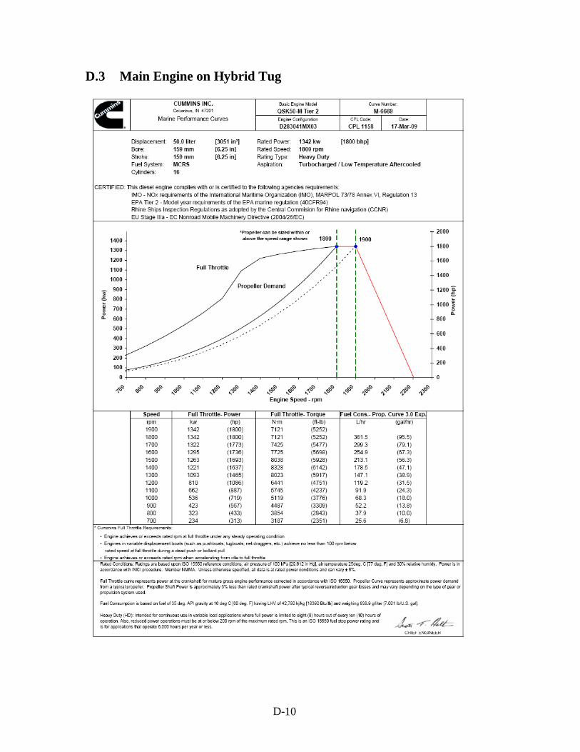
10

D.3 Main Engine on Hybrid Tug

D-

11

D-

12

D-

13

D.4 Auxiliary Engine on Hybrid Tug

D-

14

D-

15

D-

1

Appendix E – Fuel Analysis Results

E-

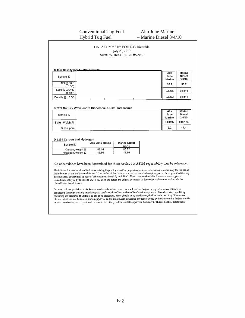
2

Conventional Tug Fuel – Alta June Marine

Hybrid Tug Fuel – Marine Diesel 3/4/10

E-

evaluating emission benefits of a hybrid tug boat · evaluating emission benefits of a hybrid tug...

Documents