tex basics tug
DESCRIPTION
TEX lecturesTRANSCRIPT
The Concept of . . .
A Short . . .
What is LATEX then?
Getting Started
Title Page
ðð ññ
ð ñ
Page 1 of 12
Go Back
Full Screen
Close
Quit
Indian TEX Users GroupURL: http://www.river-valley.com/tug
On-line Tutorial on LATEX
The Tutorial TeamIndian TEX Users Group, sjp Buildings, Cotton Hills
Trivandrum 695014, india2000
Prof. (Dr.) K. S. S. Nambooripad, Director, Center for Mathematical Sciences, Trivandrum, (Editor);Dr. E. Krishnan, Reader in Mathematics, University College, Trivandrum; T. Rishi, Focal Image (India)Pvt. Ltd., Trivandrum; L. A. Ajith, Focal Image (India) Pvt. Ltd., Trivandrum; A. M. Shan, Focal Image
(India) Pvt. Ltd., Trivandrum; C. V. Radhakrishnan, River Valley Technologies, Software TechnologyPark, Trivandrum constitute the TUGIndia Tutorial team
This document is generated from LATEX sources compiled with pdfLATEX v. 14ein an INTEL Pentium III 700 MHz system running Linux kernel version
2.2.14-12. The packages used are hyperref.sty and pdfscreen.sty
c©2000, Indian TEX Users Group. This document may be distributed under the termsof the LATEX Project Public License, as described in lppl.txt in the base LATEX
distribution, either version 1.0 or, at your option, any later version
The Concept of . . .
A Short . . .
What is LATEX then?
Getting Started
Title Page
ðð ññ
ð ñ
Page 2 of 12
Go Back
Full Screen
Close
Quit
Gentle Reader,
Generation of letter forms by mathematical means was first tried inthe fifteenth century; it became popular in the sixteenth andseventeenth centuries; and it was abandoned (for good reasons)during the eighteenth century. Perhaps the twentieth century willturn out to be the right time for this idea to make a comeback, nowthat mathematics has advanced and computers are able to do thecalculations.
Modern printing equipment based on raster lines—in which metal“type” has been replaced by purely combinatorial patterns of zeroesand ones that specify the desired position of ink in a discreteway—makes mathematics and computer science increasinglyrelevant to printing. We now have the ability to give a completelyprecise definition of letter shapes that will produce essentiallyequivalent results on all raster-based machines. Moreover, theshapes can be defined in terms of variable parameters; computerscan “draw” new fonts of characters in seconds, making it possible fordesigners to perform valuable experiments that were previouslyunthinkable.
— Donald Erwin Knuth, The METAFONT book
The Concept of . . .
A Short . . .
What is LATEX then?
Getting Started
Title Page
ðð ññ
ð ñ
Page 3 of 12
Go Back
Full Screen
Close
Quit
1 Introduction
1.1. The Concept of Generic Markup
Originally markup was the annotation of manuscripts of a copy editor telling thetypesetter how to format the manuscript. It consisted of handwritten notes suchas ‘set this heading in 12 point Helvetica italic on a 10 point body, justified on a 22pica slug with indents of 1 em on the left and none on the right.’ With the adventof computers, these marks could be coded electronically using a special codingsystem and people started inventing their own markup schemes. The followinglow level formatting commands used to instruct a computer for carriage return,center the following text, and go to the next page are a typical example:
.pa ; .sp 2 ; .ce ; .bdTitle of the chapter.sp
In another markup scheme it will be like as given hereunder:
\vfill\eject\begingroup\bf\obeylines\vskip 20pt\hfil Title of the chapter\vskip 10pt\endgroup\bigskip
The Concept of . . .
A Short . . .
What is LATEX then?
Getting Started
Title Page
ðð ññ
ð ñ
Page 4 of 12
Go Back
Full Screen
Close
Quit
Documents created with such specific markup became difficult for typesetting sys-tems to cope up. A movement was started to create a standard markup language,which all typesetting vendors would be persuaded to accept as input. Thus camethe Generic Markup Language (gml) which later on developed into Standard Gen-eralized Markup Language (sgml) and now a subset of which known as ExtensibleMarkup Language (xml) is poised to take up the World Wide Web.
However, the development of sgml moved towards representing the documentsin an exchangeable format aiming at ‘publishing in its broadest sense, rangingfrom single medium conventional publishing to multimedia data base publishing’.sgml can also be used in office document processing when the benefits of humanreadability and interchange with publishing systems as required. It is a meta-language for defining infinite variety of markup languages and is not concernedwith the formatting of marked-up documents., i.e., there is no layout tags.
This void is filled by the advent of TEX which combines the balance of genericmarkup and layout specific support. The class file mechanism followed in LATEXmakes it possible to produce the same source document in different layouts, whileenough bells and whistles are available to fine-tune important documents for pro-ducing the highest quality.
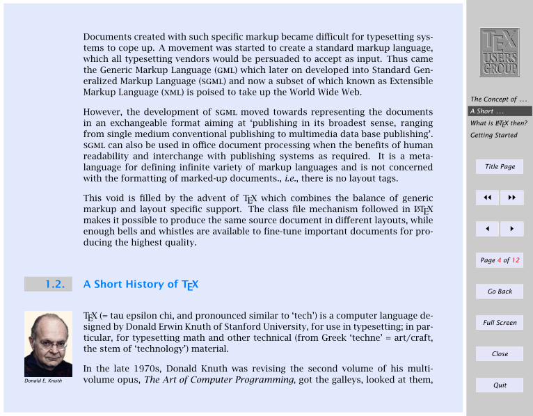
1.2. A Short History of TEX
Donald E. Knuth
TEX (= tau epsilon chi, and pronounced similar to ‘tech’) is a computer language de-signed by Donald Erwin Knuth of Stanford University, for use in typesetting; in par-ticular, for typesetting math and other technical (from Greek ‘techne’ = art/craft,the stem of ‘technology’) material.
In the late 1970s, Donald Knuth was revising the second volume of his multi-volume opus, The Art of Computer Programming, got the galleys, looked at them,
The Concept of . . .
A Short . . .
What is LATEX then?
Getting Started
Title Page
ðð ññ
ð ñ
Page 5 of 12
Go Back
Full Screen
Close
Quit
and said (approximately) ‘bleccch’! he had just received his first samples of thenew computer typesetting, and its quality was so far below that of the first editionof Volume 2 that he couldn’t stand it. He thought for awhile, and said (approxi-mately), “I’m a computer scientist; I ought to be able to do something about this”,so he set out to learn what were the traditional rules for typesetting math, whatconstituted good typography, and (because the fonts of symbols that he neededreally didn’t exist) as much as he could about type design. He figured this wouldtake about 6 months. (Ultimately, it took nearly 10 years, but along the way he hadlots of help from some people who should be well known to readers of this list –Hermann Zapf, Chuck Bigelow, Kris Holmes, Matthew Carter and Richard Southallare acknowledged in the introduction to Volume E, Computer Modern Typefaces,of the Addison-Wesley Computers & Typesetting book series.)
A year or so after he started, Knuth was invited by the American MathematicalSociety (ams) to present one of the principal invited lectures at their annual meet-ing. This honor is awarded to significant academic researchers who (mostly) weretrained as mathematicians, but who have done most of their work in not strictlymathematical areas (there are a number of physicists, astronomers, etc., in the an-nals of this lecture series as well as computer scientists); the lecturer can speakon any topic (s)he wishes, and Knuth decided to speak on computer science in theservice of mathematics. The topic he presented was his new work on TEX (for type-setting) and METAFONT (for developing fonts for use with TEX). He presented notonly the roots of the typographical concepts, but also the mathematical notions(e.g., the use of bezier splines to shape glyphs) on which these two programs arebased. The programs sounded like they were just about ready to use, and quitea few mathematicians, including the chair of the Mathematical Society’s board oftrustees, decided to take a closer look. As it turned out, TEX was still a lot closerto a research project than to an industrial strength product, but there were certainattractive features:
it was intended to be used directly by authors (and their secretaries) who are
The Concept of . . .
A Short . . .
What is LATEX then?
Getting Started
Title Page
ðð ññ
ð ñ
Page 6 of 12
Go Back
Full Screen
Close
Quit
the ones who really know what they are writing about;
it came from an academic source, and was intended to be available for nomonetary fee (nobody said anything about how much support it was going toneed);
as things developed, it became available on just about any computer and oper-ating system, and was designed specifically so that input files (files containingmarkup instructions; this is not a wysiwyg system) would be portable, andwould generate the same output on any system on which they were processed– same hyphenations, line breaks, page breaks, etc., etc.;
other programs available at the time for mathematical composition were:? proprietary? very expensive? often limited to specific hardware? if wysiwyg, the same expression in two places in the same document
might very well not look the same, never mind look the same if processedon two different systems.
Mathematicians are traditionally, shall we say, frugal; their budgets have not beenlarge (before computer algebra systems, pencils, paper, chalk and blackboardswere the most important research tools). TEX came along just before the begin-nings of the personal computer; although it was developed on one of the last ofthe ‘academic’ mainframes (the decsystem (Edusystem)-10 and -20), it was veryquickly ported to some early hp workstations and, as they emerged, the new per-sonal systems. From the start, it has been popular among mathematicians, physi-cists, astrophysicists, astronomers, any research scientists who were plagued bylack of the necessary symbols on typewriters and who wanted a more professionallook to their preprints.
To produce his own books, Knuth had to tackle all the paraphernalia of academicpublishing—footnotes, floating insertions (figures and tables), etc. As a mathe-matician/computer scientist, he developed an input language that makes sense
The Concept of . . .
A Short . . .
What is LATEX then?
Getting Started
Title Page
ðð ññ
ð ñ
Page 7 of 12
Go Back
Full Screen
Close
Quit
to other scientists, and for math expressions, is quite similar to how one mathe-matician would recite a string of notation to another on the telephone. The TEXlanguage is an interpreter. It accepts mixed commands and data. The commandlanguage is very low level (skip so much space, change to font X, set this stringof words in paragraph form, . . . ), but is amenable to being enhanced by definingmacro commands to build a very high level user interface (this is the title, this isthe author, use them to set a title page according to ams specifications). The han-dling of footnotes and similar structures are so well behaved that ‘style files’ havebeen created for TEX to process critical editions and legal tomes. It is also (aftersome highly useful enhancements in about 1990) able to handle the compositionof many different languages according to their own traditional rules, and is for thisreason (as well as for the low cost), quite widely used in eastern Europe.
Some of the algorithms in TEX have not been bettered in any of the compositiontools devised in the years since TEX appeared. The most obvious example is theparagraph breaking: text is considered a full paragraph at a time, not line-by-line;this is the basic starting algorithm used in the hz-program by Peter Karow (andnamed for Hermann Zapf, who developed the special fonts this program needs toimprove on the basics).
In summary, TEX is a special-purpose programming language that is the center-piece of a typesetting system that produces publication quality mathematics (andsurrounding text), available to and usable by individuals.
1.3. What is LATEX then?
At the beginning of 1980s, Leslie Lamport started work on a document prepara-tion system called LATEX based on the TEX formatter. This system adds a set offunctions that makes the TEX language more friendlier than using the primitives
The Concept of . . .
A Short . . .
What is LATEX then?
Getting Started
Title Page
ðð ññ
ð ñ
Page 8 of 12
Go Back
Full Screen
Close
Quit
provided in TEX, enabling the author to concentrate on the content and structureof the document rather than the formatting details, so that the author might notloose the train of thought while writing his document. Also, LATEX’s functionality,in conjunction with a few auxiliary programs, includes the generation of indices,bibliographies, cross-references, tables of contents, graphic inclusion, etc. Theseare the features that are lacking in basic TEX (usually called plain TEX).
1.4. Getting Started
First of all, let’s see what steps are necessary to produce a document using LATEX.The first step is to type the file that LATEX reads. This is usually called the LATEX fileor the input file, and it can be created using a simple text editor (in fact, if you’reusing a fancy word processor, you have to be sure that your file is saved in asciior non-document mode without any special control characters). The LATEX programthen reads your input file and produces what is called a dvi file (dvi stands forDeVice Independent). This file is not readable, at least not by humans. The dvi fileis then read by another program (called a device driver) that produces the outputthat is readable by humans. Why the extra file? The same dvi file can be read bydifferent device drivers to produce output on a dot matrix printer, a laser printer,a screen viewer, or a phototypesetter. Once you have produced a dvi file thatgives the right output on, say, a screen viewer, you can be assured that you willget exactly the same output on a laser printer without running the LATEX programagain.
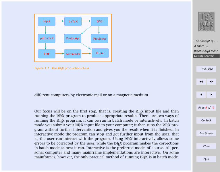
The process may be thought of as given in the Figure 1.1. This means that wedon’t see our output in its final form when it is being typed at the terminal. Butin this case a little patience is amply rewarded, for a large number of symbols notavailable in most word processing programs become available. In addition, thetypesetting is done with more precision, and the input files are easily sent between
The Concept of . . .
A Short . . .
What is LATEX then?
Getting Started
Title Page
ðð ññ
ð ñ
Page 9 of 12
Go Back
Full Screen
Close
Quit
DVI
Printer
Input LaTeX
pdfLaTeX PostScript
Acroreader
Previewer
Figure 1.1 The LATEX production chain
different computers by electronic mail or on a magnetic medium.
Our focus will be on the first step, that is, creating the LATEX input file and thenrunning the LATEX program to produce appropriate results. There are two ways ofrunning the LATEX program; it can be run in batch mode or interactively. In batchmode you submit your LATEX input file to your computer; it then runs the LATEX pro-gram without further intervention and gives you the result when it is finished. Ininteractive mode the program can stop and get further input from the user, thatis, the user can interact with the program. Using LATEX interactively allows someerrors to be corrected by the user, while the LATEX program makes the correctionsin batch mode as best it can. Interactive is the preferred mode, of course. All per-sonal computer and many mainframe implementations are interactive. On somemainframes, however, the only practical method of running LATEX is in batch mode.
The Concept of . . .
A Short . . .
What is LATEX then?
Getting Started
Title Page
ðð ññ
ð ñ
Page 10 of 12
Go Back
Full Screen
Close
Quit
\documentclass[a4paper]tutorial\pagestyleheadings\usepackage[screen,rightpanel,paneltoc,code]pdfscreen
\begindocument
\chapterIntroduction
\sectionThe Concept of Generic MarkupOriginally markup was the annotation of manuscriptsof a copy editor telling the typesetter how to formatthe manuscript. It consisted of handwritten notes suchas ‘\emphset this heading in 12 point Helvetica
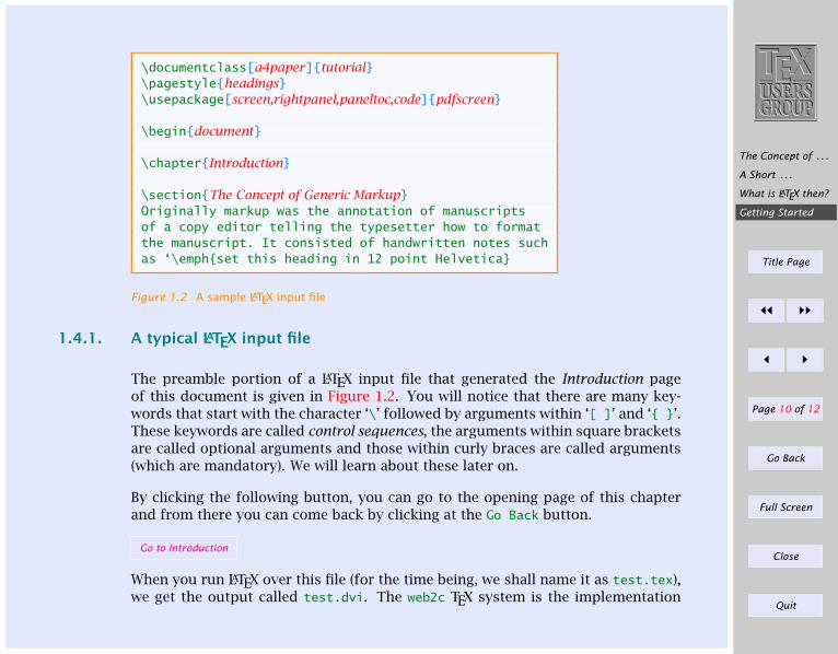
Figure 1.2 A sample LATEX input file
1.4.1. A typical LATEX input file
The preamble portion of a LATEX input file that generated the Introduction pageof this document is given in Figure 1.2. You will notice that there are many key-words that start with the character ‘\’ followed by arguments within ‘[ ]’ and ‘ ’.These keywords are called control sequences, the arguments within square bracketsare called optional arguments and those within curly braces are called arguments(which are mandatory). We will learn about these later on.
By clicking the following button, you can go to the opening page of this chapterand from there you can come back by clicking at the Go Back button.
Go to Introduction
When you run LATEX over this file (for the time being, we shall name it as test.tex),we get the output called test.dvi. The web2c TEX system is the implementation
The Concept of . . .
A Short . . .
What is LATEX then?
Getting Started
Title Page
ðð ññ
ð ñ
Page 11 of 12
Go Back
Full Screen
Close
Quit
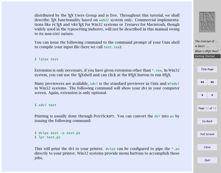
distributed by the TEX Users Group and is free. Throughout this tutorial, we shalldescribe TEX functionality based on web2c system only. Commercial implementa-tions like pcTEX and y&yTEX for Win32 systems or Textures for Macintosh, thoughwidely used in the typesetting industry, will not be described in this manual owingto its non-gnu nature.
You can issue the following command to the command prompt of your Unix shellto compile your input file (here we call test.tex):
$ latex test
Extension is only necessary, if you have given extension other than *.tex. In Win32system, you can use the TEXshell and can click at the LATEX button to run LATEX.
Many previewers are available, xdvi is the standard previewer in Unix and Windviin Win32 systems. The following command will show your dvi in your computerscreen. Again, extension is only optional.
$ xdvi test
Printing is usually done through PostScript. You can convert the dvi into ps byissuing the following command:
$ dvips test -o test.ps$ lpr test.ps
This will print the dvi to your printer. dvips can be configured to pipe the *.psdirectly to your printer. Win32 systems provide menu buttons to accomplish thesejobs.
The Concept of . . .
A Short . . .
What is LATEX then?
Getting Started
Title Page
ðð ññ
ð ñ
Page 12 of 12
Go Back
Full Screen
Close
Quit
You might be amused to know that this test.dvi is independent of any platformand devices. You can view this output in any dvi previewer of any operating sys-tem irrespective of the os of origination and can be printed in any printer for theidentical output, which is not the case with the wysiwyg typesetting systems thatare usually hard wired to the installed printer, the format changes as soon as youchange your printer. Therefore, TEX is device and platform independent. Also youcan compile the very same TEX sources in any TEX system in any operating sys-tem irrespective of its originating os. This platform independence has made TEXdocuments a choice of transfer, especially scientific documents over the internet.
TEX Directory . . .
Fonts
Characters
Epilog
Title Page
ðð ññ
ð ñ
Page 1 of 10
Go Back
Full Screen
Close
Quit
Indian TEX Users GroupURL: http://www.river-valley.com/tug
2On-line Tutorial on LATEX
The Tutorial TeamIndian TEX Users Group, sjp Buildings, Cotton Hills
Trivandrum 695014, india2000
Prof. (Dr.) K. S. S. Nambooripad, Director, Center for Mathematical Sciences, Trivandrum, (Editor);Dr. E. Krishnan, Reader in Mathematics, University College, Trivandrum; T. Rishi, Focal Image (India)Pvt. Ltd., Trivandrum; L. A. Ajith, Focal Image (India) Pvt. Ltd., Trivandrum; A. M. Shan, Focal Image
(India) Pvt. Ltd., Trivandrum; C. V. Radhakrishnan, River Valley Technologies, Software TechnologyPark, Trivandrum constitute the TUGIndia Tutorial team
This document is generated from LATEX sources compiled with pdfLATEX v. 14ein an INTEL Pentium III 700 MHz system running Linux kernel version
2.2.14-12. The packages used are hyperref.sty and pdfscreen.sty
c©2000, Indian TEX Users Group. This document may be distributed under the termsof the LATEX Project Public License, as described in lppl.txt in the base LATEX
distribution, either version 1.0 or, at your option, any later version
TEX Directory . . .
Fonts
Characters
Epilog
Title Page
ðð ññ
ð ñ
Page 2 of 10
Go Back
Full Screen
Close
Quit
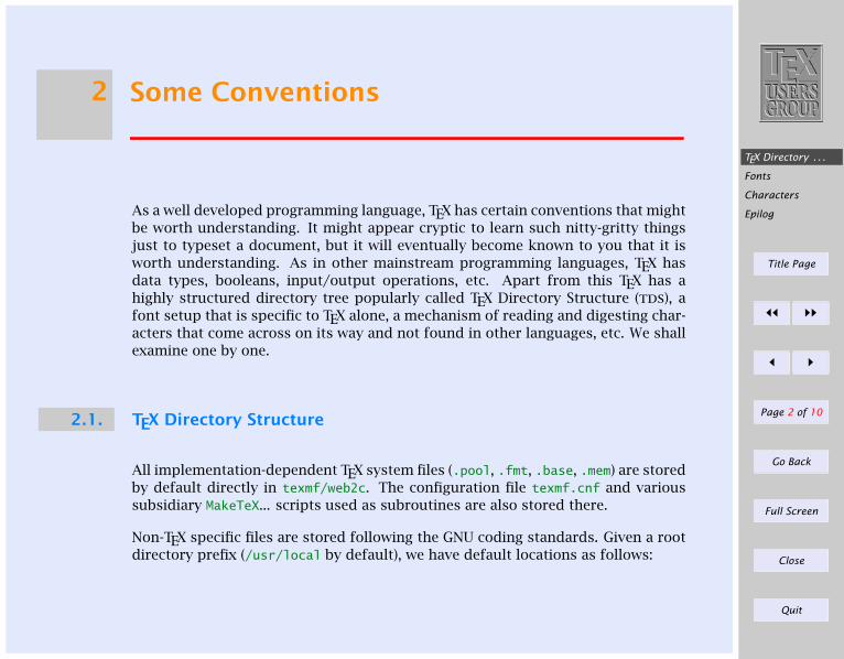
2 Some Conventions
As a well developed programming language, TEX has certain conventions that mightbe worth understanding. It might appear cryptic to learn such nitty-gritty thingsjust to typeset a document, but it will eventually become known to you that it isworth understanding. As in other mainstream programming languages, TEX hasdata types, booleans, input/output operations, etc. Apart from this TEX has ahighly structured directory tree popularly called TEX Directory Structure (tds), afont setup that is specific to TEX alone, a mechanism of reading and digesting char-acters that come across on its way and not found in other languages, etc. We shallexamine one by one.
2.1. TEX Directory Structure
All implementation-dependent TEX system files (.pool, .fmt, .base, .mem) are storedby default directly in texmf/web2c. The configuration file texmf.cnf and varioussubsidiary MakeTeX... scripts used as subroutines are also stored there.
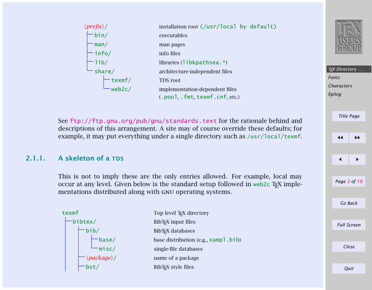
Non-TEX specific files are stored following the GNU coding standards. Given a rootdirectory prefix (/usr/local by default), we have default locations as follows:
TEX Directory . . .
Fonts
Characters
Epilog
Title Page
ðð ññ
ð ñ
Page 3 of 10
Go Back
Full Screen
Close
Quit
〈prefix〉/ installation root (/usr/local by default)
bin/ executables
man/ man pages
info/ info files
lib/ libraries (libkpathsea.*)
share/ architecture-independent files
texmf/ TDS root
web2c/ implementation-dependent files
(.pool, .fmt, texmf.cnf, etc.)
See ftp://ftp.gnu.org/pub/gnu/standards.text for the rationale behind anddescriptions of this arrangement. A site may of course override these defaults; forexample, it may put everything under a single directory such as /usr/local/texmf.
2.1.1. A skeleton of a TDS
This is not to imply these are the only entries allowed. For example, local mayoccur at any level. Given below is the standard setup followed in web2c TEX imple-mentations distributed along with gnu operating systems.
texmf Top level TEX directory
bibtex/ BibTEX input files
bib/ BibTEX databases
base/ base distribution (e.g., xampl.bib)
misc/ single-file databases
〈package〉/ name of a package
bst/ BibTEX style files
TEX Directory . . .
Fonts
Characters
Epilog
Title Page
ðð ññ
ð ñ
Page 4 of 10
Go Back
Full Screen
Close
Quit
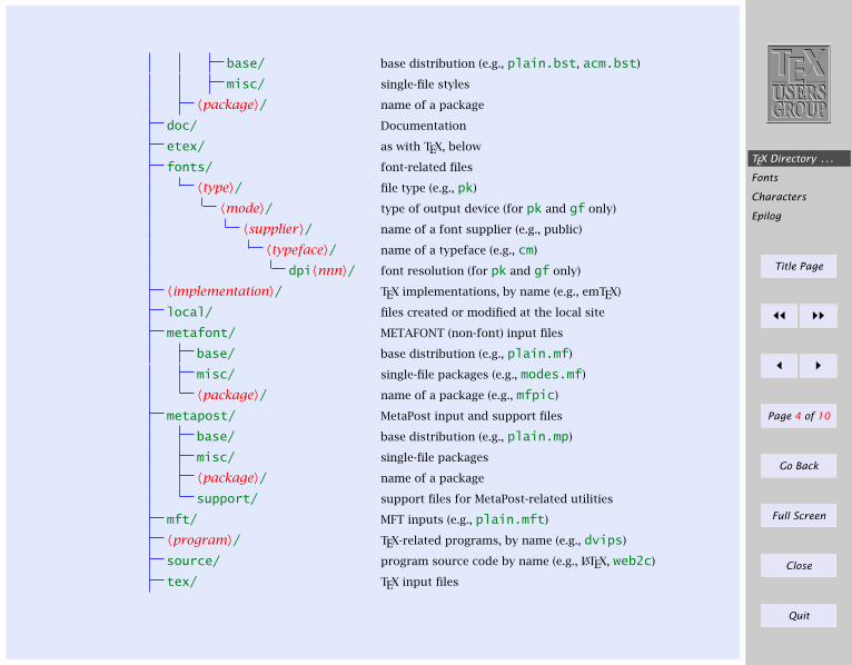
base/ base distribution (e.g., plain.bst, acm.bst)
misc/ single-file styles
〈package〉/ name of a package
doc/ Documentation
etex/ as with TEX, below
fonts/ font-related files
〈type〉/ file type (e.g., pk)
〈mode〉/ type of output device (for pk and gf only)
〈supplier〉/ name of a font supplier (e.g., public)
〈typeface〉/ name of a typeface (e.g., cm)
dpi〈nnn〉/ font resolution (for pk and gf only)
〈implementation〉/ TEX implementations, by name (e.g., emTEX)
local/ files created or modified at the local site
metafont/ METAFONT (non-font) input files
base/ base distribution (e.g., plain.mf)
misc/ single-file packages (e.g., modes.mf)
〈package〉/ name of a package (e.g., mfpic)
metapost/ MetaPost input and support files
base/ base distribution (e.g., plain.mp)
misc/ single-file packages
〈package〉/ name of a package
support/ support files for MetaPost-related utilities
mft/ MFT inputs (e.g., plain.mft)
〈program〉/ TEX-related programs, by name (e.g., dvips)
source/ program source code by name (e.g., LATEX, web2c)
tex/ TEX input files
TEX Directory . . .
Fonts
Characters
Epilog
Title Page
ðð ññ
ð ñ
Page 5 of 10
Go Back
Full Screen
Close
Quit
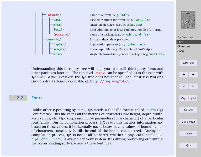
〈format〉/ name of a format (e.g., latex)
base/ base distribution for format (e.g., latex.ltx)
misc/ single-file packages (e.g., webmac.tex)
local/ local additions to or local configuration files for format
〈package〉/ name of a package (e.g., graphics, mfnfss)
generic/ format-independent packages
hyphen/ hyphenation patterns (e.g., hyphen.tex)
images/ image input files (e.g., Encapsulated PostScript)
misc/ single-file format-independent packages (e.g., null.tex).
Understanding this directory tree will help you to install third party fonts andother packages later on. The top level 〈prefix〉 can be specified as is the case withTEXLive cdrom. However, the TEX tree does not change. The latest tds WorkingGroup’s draft release is available at: http://tug.org/tds/.
2.2. Fonts
Unlike other typesetting systems, TEX needs a font file format called, *.tfm (TEXFont Metric). This file keeps all the metrics of characters like height, depth, width,kern values, etc. (TEX keeps around 64 parameters for a character) of a particularfont family. During compilation process, TEX reads this metrics information andbased on these values, it horizontally packs boxes having values of bounding boxof characters consecutively till the end of the line is encountered. During thiscompilation process, TEX is not at all bothered, whether a physical font file (like*.pfb or *.ttf etc.) is available in your system. It is during previewing or printing,the corresponding software needs these font files.
TEX Directory . . .
Fonts
Characters
Epilog
Title Page
ðð ññ
ð ñ
Page 6 of 10
Go Back
Full Screen
Close
Quit
It arises a problem, when one tries to access third party fonts supplied by vari-ous foundries, for instance, Adobe. Foundries do not supply TEX font metric file.However, this can easily be generated with afm2tfm program supplied with yourTEX distribution and is a trivial process. We will learn about these in subsequentchapters.
2.3. Characters
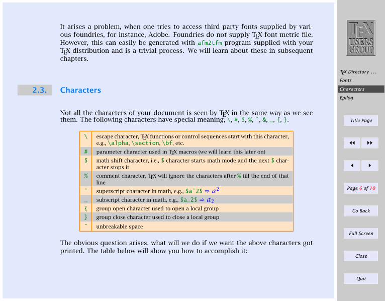
Not all the characters of your document is seen by TEX in the same way as we seethem. The following characters have special meaning, \, #, $, %, ˆ, &, _, , .
\ escape character, TEX functions or control sequences start with this character,e.g., \alpha, \section, \bf, etc.
# parameter character used in TEX macros (we will learn this later on)
$ math shift character, i.e., $ character starts math mode and the next $ char-acter stops it
% comment character, TEX will ignore the characters after % till the end of thatline
ˆ superscript character in math, e.g., $aˆ2$⇒ a2
_ subscript character in math, e.g., $a_2$⇒ a2
group open character used to open a local group
group close character used to close a local group
˜ unbreakable space
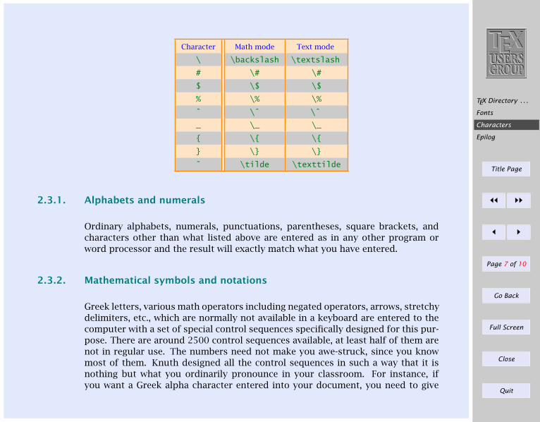
The obvious question arises, what will we do if we want the above characters gotprinted. The table below will show you how to accomplish it:
TEX Directory . . .
Fonts
Characters
Epilog
Title Page
ðð ññ
ð ñ
Page 7 of 10
Go Back
Full Screen
Close
Quit
Character Math mode Text mode
\ \backslash \textslash
# \# \#
$ \$ \$
% \% \%
ˆ \ˆ \ˆ
_ \_ \_
\ \
\ \
˜ \tilde \texttilde
2.3.1. Alphabets and numerals
Ordinary alphabets, numerals, punctuations, parentheses, square brackets, andcharacters other than what listed above are entered as in any other program orword processor and the result will exactly match what you have entered.
2.3.2. Mathematical symbols and notations
Greek letters, various math operators including negated operators, arrows, stretchydelimiters, etc., which are normally not available in a keyboard are entered to thecomputer with a set of special control sequences specifically designed for this pur-pose. There are around 2500 control sequences available, at least half of them arenot in regular use. The numbers need not make you awe-struck, since you knowmost of them. Knuth designed all the control sequences in such a way that it isnothing but what you ordinarily pronounce in your classroom. For instance, ifyou want a Greek alpha character entered into your document, you need to give
TEX Directory . . .
Fonts
Characters
Epilog
Title Page
ðð ññ
ð ñ
Page 8 of 10
Go Back
Full Screen
Close
Quit
as \alpha, this during compilation will give you ‘α’. Given below is an equationcomposed of such control sequences:
(α+ β)2 = α2 + β2 + 2αβ (2.1)
The following code generates the above equation which is not at all difficult forany academic to undertake.
\beginequation(\alpha + \beta)ˆ2 = \alphaˆ2 + \betaˆ2 + 2\alpha\beta
\endequation
Similarly, a wide variety of symbols are accessed with names similar to what we or-dinarily denote them. For instance, , ψ, -→,
∑, ⊆, 6⊆ are generated with \swarrow,
\psi, \longrightarrow, \sum, \subseteq, \not\subseteq. The point is that symbolsin TEX is extremely logical to follow and not much extra effort is needed to under-stand and remember them. We will learn more about math symbols, formulae andtheir spatial arrangement and constructs during the second phase of our tutorial.
2.3.3. Accented characters
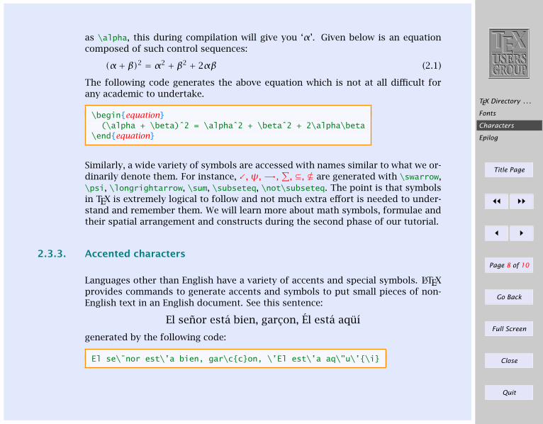
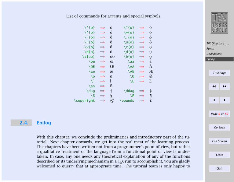
Languages other than English have a variety of accents and special symbols. LATEXprovides commands to generate accents and symbols to put small pieces of non-English text in an English document. See this sentence:
El senor esta bien, garcon, El esta aquı
generated by the following code:
El se\˜nor est\’a bien, gar\ccon, \’El est\’a aq\"u\’\i
TEX Directory . . .
Fonts
Characters
Epilog
Title Page
ðð ññ
ð ñ
Page 9 of 10
Go Back
Full Screen
Close
Quit
List of commands for accents and special symbols
\‘o =⇒ o \˜o =⇒ o\’o =⇒ o \=o =⇒ o\ˆo =⇒ o \.o =⇒ o\"o =⇒ o \uo =⇒ o\vo =⇒ o \co =⇒ o\Ho =⇒ o \do =⇒ o.\too =⇒ oo \bo =⇒ o
¯\oe =⇒ œ \aa =⇒ a\OE =⇒ Œ \AA =⇒ A\ae =⇒ æ \AE =⇒ Æ\o =⇒ ø \O =⇒ Ø\l =⇒ ł \L =⇒ Ł
\ss =⇒ ß\dag =⇒ † \ddag =⇒ ‡
\S =⇒ § \P =⇒ ¶\copyright =⇒ c© \pounds =⇒ £
2.4. Epilog
With this chapter, we conclude the preliminaries and introductory part of the tu-torial. Next chapter onwards, we get into the real meat of the learning process.The chapters have been written not from a programmer’s point of view, but rathera qualitative treatment of the language from a functional point of view is under-taken. In case, any one needs any theoretical explanation of any of the functionsdescribed or its underlying mechanism in a TEX run to accomplish it, you are gladlywelcomed to querry that at appropriate time. The tutorial team is only happy to
TEX Directory . . .
Fonts
Characters
Epilog
Title Page
ðð ññ
ð ñ
Page 10 of 10
Go Back
Full Screen
Close
Quit
explain that in great detail. So we start the LATEX document classes in the nextchapter.

Basics
LATEX Input Files
The Document
Sectioning . . .
Notes
Title Page
ðð ññ
ð ñ
Page 1 of 10
Go Back
Full Screen
Close
Quit
Indian TEX Users GroupURL: http://www.river-valley.com/tug
3On-line Tutorial on LATEX
The Tutorial TeamIndian TEX Users Group, sjp Buildings, Cotton Hills
Trivandrum 695014, india2000
Prof. (Dr.) K. S. S. Nambooripad, Director, Center for Mathematical Sciences, Trivandrum, (Editor);Dr. E. Krishnan, Reader in Mathematics, University College, Trivandrum; T. Rishi, Focal Image (India)Pvt. Ltd., Trivandrum; L. A. Ajith, Focal Image (India) Pvt. Ltd., Trivandrum; A. M. Shan, Focal Image
(India) Pvt. Ltd., Trivandrum; C. V. Radhakrishnan, River Valley Technologies, Software TechnologyPark, Trivandrum constitute the TUGIndia Tutorial team
This document is generated from LATEX sources compiled with pdfLATEX v. 14ein an INTEL Pentium III 700 MHz system running Linux kernel version
2.2.14-12. The packages used are hyperref.sty and pdfscreen.sty
c©2000, Indian TEX Users Group. This document may be distributed under the termsof the LATEX Project Public License, as described in lppl.txt in the base LATEX
distribution, either version 1.0 or, at your option, any later version
Basics
LATEX Input Files
The Document
Sectioning . . .
Notes
Title Page
ðð ññ
ð ñ
Page 2 of 10
Go Back
Full Screen
Close
Quit
3 Introduction to LATEX
LATEX is a macro package which enables authors to typeset and print their work withthe highest typographical quality, using a predefined, professional layout. Sinceits introduction, it has been periodically updated and revised, like all softwareproducts. For many years now the version number has been fixed at 2ε. In aneffort to re-establish a genuine, improved standard, the LATEX3 Project was set upin 1989. And the beta version of LATEX3 has just been released. Throughout thistutorial by LATEX, we mean LATEX2ε.
3.1. Basics
As explained in the previous chapter, LATEX is quite different from wysiwyg (whatyou see is what you get) approach which most modern word processors such msWord or Corel WordPerfect follow. With these applications, authors specify thedocument layout interactively while typing text into the computer. Along the waythey can see on the screen how the final work will look like when it is printed.
When using LATEX it is normally not possible to see the final output while typing thetext. But the final output can be previewed on the screen after processing the filewith LATEX.
Following is the method to create a LATEX document.
Basics
LATEX Input Files
The Document
Sectioning . . .
Notes
Title Page
ðð ññ
ð ñ
Page 3 of 10
Go Back
Full Screen
Close
Quit
(1) Type in the text with necessary commands.
(2) Compile the text with LATEX engine.
(3) After successful compilation of the document output can be previewed on thescreen.
3.2. LATEX Input Files
The input for LATEX is a plain ascii text file. You can create it with any text editor.It contains the text of the document as well as the commands which tells LATEX howto typeset the text. The commands start with a ‘\’ (backslash character).
Eg: \bf, \it, etc.
3.2.1. LATEX input file structure
When LATEX2ε process an input file, it requires us to follow a certain structure.Thus every input file must start with the command
\documentclassclass
When all the set up work is done, you start the body of the text with the command
\begindocument
Now you enter the text mixed with some useful LATEX commands. At the end of thedocument you add the following command
Basics
LATEX Input Files
The Document
Sectioning . . .
Notes
Title Page
ðð ññ
ð ñ
Page 4 of 10
Go Back
Full Screen
Close
Quit
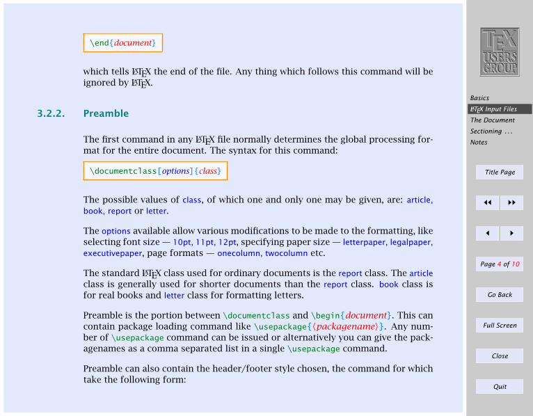
\enddocument
which tells LATEX the end of the file. Any thing which follows this command will beignored by LATEX.
3.2.2. Preamble
The first command in any LATEX file normally determines the global processing for-mat for the entire document. The syntax for this command:
\documentclass[options]class
The possible values of class, of which one and only one may be given, are: article,book, report or letter.
The options available allow various modifications to be made to the formatting, likeselecting font size — 10pt, 11pt, 12pt, specifying paper size — letterpaper, legalpaper,executivepaper, page formats — onecolumn, twocolumn etc.
The standard LATEX class used for ordinary documents is the report class. The articleclass is generally used for shorter documents than the report class. book class isfor real books and letter class for formatting letters.
Preamble is the portion between \documentclass and \begindocument. This cancontain package loading command like \usepackage〈packagename〉. Any num-ber of \usepackage command can be issued or alternatively you can give the pack-agenames as a comma separated list in a single \usepackage command.
Preamble can also contain the header/footer style chosen, the command for whichtake the following form:
Basics
LATEX Input Files
The Document
Sectioning . . .
Notes
Title Page
ðð ññ
ð ñ
Page 5 of 10
Go Back
Full Screen
Close
Quit
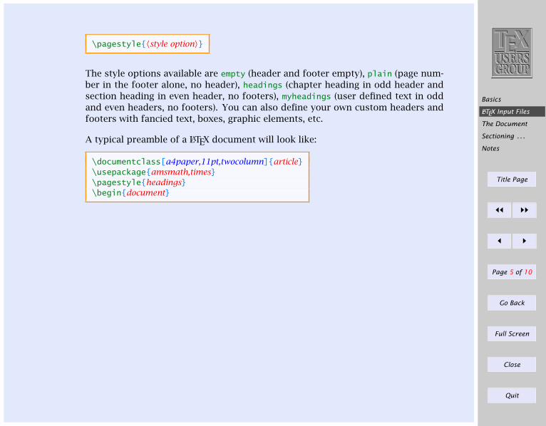
\pagestyle〈style option〉
The style options available are empty (header and footer empty), plain (page num-ber in the footer alone, no header), headings (chapter heading in odd header andsection heading in even header, no footers), myheadings (user defined text in oddand even headers, no footers). You can also define your own custom headers andfooters with fancied text, boxes, graphic elements, etc.
A typical preamble of a LATEX document will look like:
\documentclass[a4paper,11pt,twocolumn]article\usepackageamsmath,times\pagestyleheadings\begindocument
Basics
LATEX Input Files
The Document
Sectioning . . .
Notes
Title Page
ðð ññ
ð ñ
Page 6 of 10
Go Back
Full Screen
Close
Quit
3.3. The Document
A LATEX document has broadly three parts viz., frontmatter, mainmatter and back-matter.
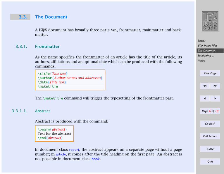
3.3.1. Frontmatter
As the name specifies the frontmatter of an article has the title of the article, itsauthors, affiliations and an optional date which can be produced with the followingcommands.
\titleTitle text\authorAuthor names and addresses\dateDate text\maketitle
The \maketitle command will trigger the typesetting of the frontmatter part.
3.3.1.1. Abstract
Abstract is produced with the command:
\beginabstractText for the abstract\endabstract
In document class report, the abstract appears on a separate page without a pagenumber; in article, it comes after the title heading on the first page. An abstract isnot possible in document class book.
Basics
LATEX Input Files
The Document
Sectioning . . .
Notes
Title Page
ðð ññ
ð ñ
Page 7 of 10
Go Back
Full Screen
Close
Quit
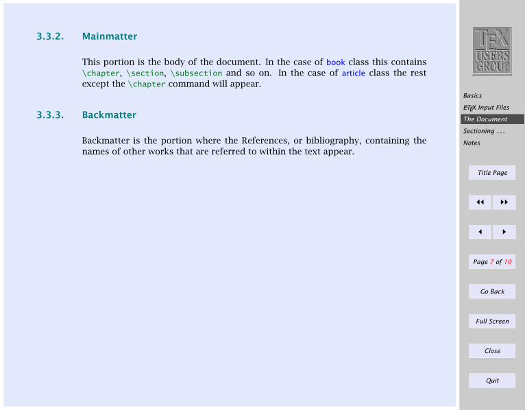
3.3.2. Mainmatter
This portion is the body of the document. In the case of book class this contains\chapter, \section, \subsection and so on. In the case of article class the restexcept the \chapter command will appear.
3.3.3. Backmatter
Backmatter is the portion where the References, or bibliography, containing thenames of other works that are referred to within the text appear.
Basics
LATEX Input Files
The Document
Sectioning . . .
Notes
Title Page
ðð ññ
ð ñ
Page 8 of 10
Go Back
Full Screen
Close
Quit
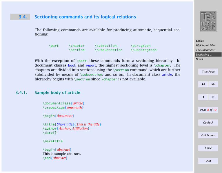
3.4. Sectioning commands and its logical relations
The following commands are available for producing automatic, sequential sec-tioning:
\part \chapter \subsection \paragraph\section \subsubsection \subparagraph
With the exception of \part, these commands form a sectioning hierarchy. Indocument classes book and report, the highest sectioning level is \chapter. Thechapters are divided into sections using the \section command, which are furthersubdivided by means of \subsection, and so on. In document class article, thehierarchy begins with \section since \chapter is not available.
3.4.1. Sample body of article
\documentclassarticle\usepackageamsmath
\begindocument
\title[Short title]This is the title\authorAuthor, Affiliation\date
\maketitle
\beginabstractThis is sample abstract.\endabstract
Basics
LATEX Input Files
The Document
Sectioning . . .
Notes
Title Page
ðð ññ
ð ñ
Page 9 of 10
Go Back
Full Screen
Close
Quit
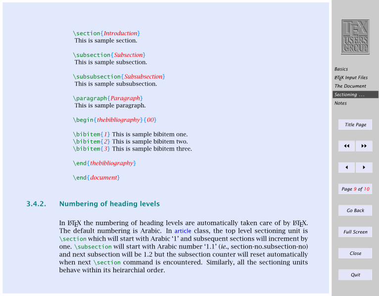
\sectionIntroductionThis is sample section.
\subsectionSubsectionThis is sample subsection.
\subsubsectionSubsubsectionThis is sample subsubsection.
\paragraphParagraphThis is sample paragraph.
\beginthebibliography00
\bibitem1 This is sample bibitem one.\bibitem2 This is sample bibitem two.\bibitem3 This is sample bibitem three.
\endthebibliography
\enddocument
3.4.2. Numbering of heading levels
In LATEX the numbering of heading levels are automatically taken care of by LATEX.The default numbering is Arabic. In article class, the top level sectioning unit is\section which will start with Arabic ‘1’ and subsequent sections will increment byone. \subsection will start with Arabic number ‘1.1’ (ie., section-no.subsection-no)and next subsection will be 1.2 but the subsection counter will reset automaticallywhen next \section command is encountered. Similarly, all the sectioning unitsbehave within its heirarchial order.
Basics
LATEX Input Files
The Document
Sectioning . . .
Notes
Title Page
ðð ññ
ð ñ
Page 10 of 10
Go Back
Full Screen
Close
Quit
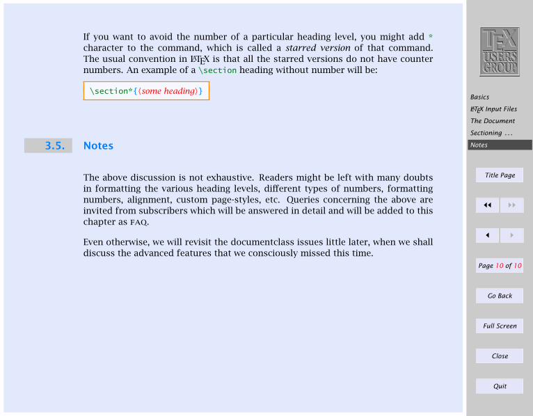
If you want to avoid the number of a particular heading level, you might add *character to the command, which is called a starred version of that command.The usual convention in LATEX is that all the starred versions do not have counternumbers. An example of a \section heading without number will be:
\section*〈some heading〉
3.5. Notes
The above discussion is not exhaustive. Readers might be left with many doubtsin formatting the various heading levels, different types of numbers, formattingnumbers, alignment, custom page-styles, etc. Queries concerning the above areinvited from subscribers which will be answered in detail and will be added to thischapter as faq.
Even otherwise, we will revisit the documentclass issues little later, when we shalldiscuss the advanced features that we consciously missed this time.
Lists
Displayed text
Title Page
ðð ññ
ð ñ
Page 1 of 8
Go Back
Full Screen
Close
Quit
Indian TEX Users GroupURL: http://www.river-valley.com/tug
4On-line Tutorial on LATEX
The Tutorial TeamIndian TEX Users Group, sjp Buildings, Cotton Hills
Trivandrum 695014, india2000
Prof. (Dr.) K. S. S. Nambooripad, Director, Center for Mathematical Sciences, Trivandrum, (Editor);Dr. E. Krishnan, Reader in Mathematics, University College, Trivandrum; T. Rishi, Focal Image (India)Pvt. Ltd., Trivandrum; L. A. Ajith, Focal Image (India) Pvt. Ltd., Trivandrum; A. M. Shan, Focal Image
(India) Pvt. Ltd., Trivandrum; C. V. Radhakrishnan, River Valley Technologies, Software TechnologyPark, Trivandrum constitute the TUGIndia Tutorial team
This document is generated from LATEX sources compiled with pdfLATEX v. 14ein an INTEL Pentium III 700 MHz system running Linux kernel version
2.2.14-12. The packages used are hyperref.sty and pdfscreen.sty
c©2000, Indian TEX Users Group. This document may be distributed under the termsof the LATEX Project Public License, as described in lppl.txt in the base LATEX
distribution, either version 1.0 or, at your option, any later version
Lists
Displayed text
Title Page
ðð ññ
ð ñ
Page 2 of 8
Go Back
Full Screen
Close
Quit
4 Lists, etc.
4.1. Lists
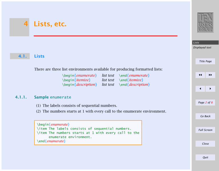
There are three list environments available for producing formatted lists:
\beginenumerate list text \endenumerate\beginitemize list text \enditemize\begindescription list text \enddescription
4.1.1. Sample enumerate
(1) The labels consists of sequential numbers.
(2) The numbers starts at 1 with every call to the enumerate environment.
\beginenumerate\item The labels consists of sequential numbers.\item The numbers starts at 1 with every call to the
enumerate environment.\endenumerate
Lists
Displayed text
Title Page
ðð ññ
ð ñ
Page 3 of 8
Go Back
Full Screen
Close
Quit
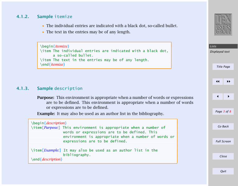
4.1.2. Sample itemize
• The individual entries are indicated with a black dot, so-called bullet.
• The text in the entries may be of any length.
\beginitemize\item The individual entries are indicated with a black dot,
a so-called bullet.\item The text in the entries may be of any length.\enditemize
4.1.3. Sample description
Purpose: This environment is appropriate when a number of words or expressionsare to be defined. This environment is appropriate when a number of wordsor expressions are to be defined.
Example: It may also be used as an author list in the bibliography.
\begindescription\item[Purpose:] This environment is appropriate when a number of
words or expressions are to be defined. Thisenvironment is appropriate when a number of words orexpressions are to be defined.
\item[Example:] It may also be used as an author list in thebibliography.
\enddescription
Lists
Displayed text
Title Page
ðð ññ
ð ñ
Page 4 of 8
Go Back
Full Screen
Close
Quit
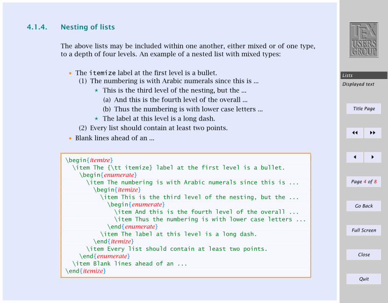
4.1.4. Nesting of lists
The above lists may be included within one another, either mixed or of one type,to a depth of four levels. An example of a nested list with mixed types:
• The itemize label at the first level is a bullet.(1) The numbering is with Arabic numerals since this is ...
? This is the third level of the nesting, but the ...
(a) And this is the fourth level of the overall ...
(b) Thus the numbering is with lower case letters ...
? The label at this level is a long dash.
(2) Every list should contain at least two points.
• Blank lines ahead of an ...
\beginitemize\item The \tt itemize label at the first level is a bullet.\beginenumerate\item The numbering is with Arabic numerals since this is ...
\beginitemize\item This is the third level of the nesting, but the ...
\beginenumerate\item And this is the fourth level of the overall ...\item Thus the numbering is with lower case letters ...
\endenumerate\item The label at this level is a long dash.
\enditemize\item Every list should contain at least two points.
\endenumerate\item Blank lines ahead of an ...
\enditemize
Lists
Displayed text
Title Page
ðð ññ
ð ñ
Page 5 of 8
Go Back
Full Screen
Close
Quit
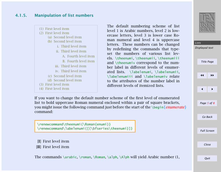
4.1.5. Manipulation of list numbers
(1) First level item(2) First level item
(a) Second level item(b) Second level item
i. Third level item
ii. Third level item
A. Fourth level item
B. Fourth level item
iii. Third level item
iv. Third level item
(c) Second level item(d) Second level item
(3) First level item(4) First level item
The default numbering scheme of listlevel 1 is Arabic numbers, level 2 is low-ercase letters, level 3 is lower case Ro-man numeral and level 4 is uppercaseletters. These numbers can be changedby redefining the commands that type-set the numbers of various list lev-els. \theenumi, \theenumii, \theenumiiiand \theenumiv correspond to the num-ber label in different levels of enumer-ated lists. \labelenumi, \labelenumii,\labelenumiii and \labelenumiv relateto the attributes of the number label indifferent levels of itemized lists.
If you want to change the default number scheme of the first level of enumeratedlist to bold uppercase Roman numeral enclosed within a pair of square brackets,you might issue the following command just before the start of the \beginenumeratecommand:
\renewcommand\theenumi\Romanenumi\renewcommand\labelenumi[\bfseries\theenumi]
[I] First level item
[II] First level item
The commands \arabic, \roman, \Roman, \alph, \Alph will yield Arabic number (1,
Lists
Displayed text
Title Page
ðð ññ
ð ñ
Page 6 of 8
Go Back
Full Screen
Close
Quit
2, 3, . . . ), lowercase Roman numeral (i, ii, iii, . . . ), uppercase Roman numeral (I,II, III, . . . ), lowercase alphabet (a, b, c, . . . ) and uppercase alphabet (A, B, C, . . . )respectively.
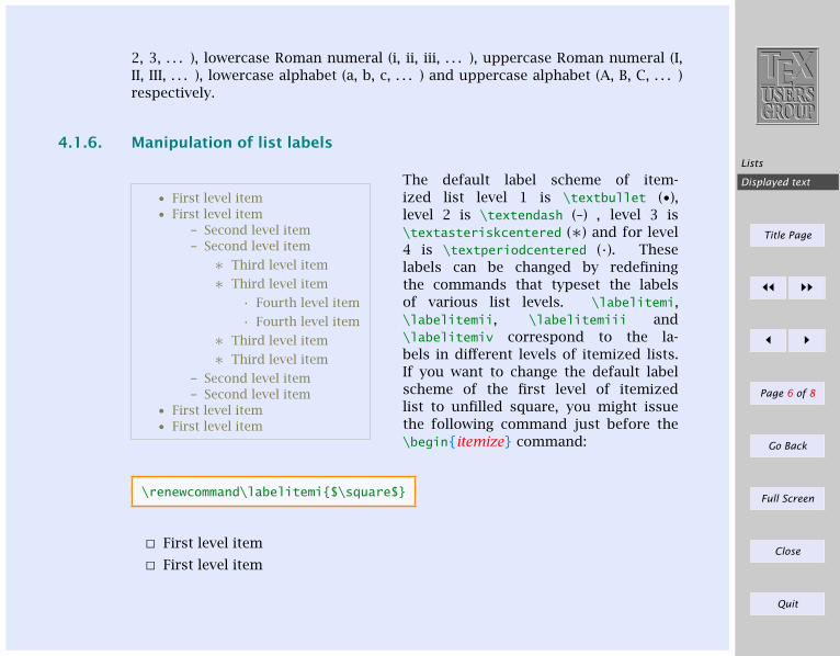
4.1.6. Manipulation of list labels
• First level item• First level item
– Second level item– Second level item
∗ Third level item
∗ Third level item
· Fourth level item
· Fourth level item
∗ Third level item
∗ Third level item
– Second level item– Second level item
• First level item• First level item
The default label scheme of item-ized list level 1 is \textbullet (•),level 2 is \textendash (–) , level 3 is\textasteriskcentered (∗) and for level4 is \textperiodcentered (·). Theselabels can be changed by redefiningthe commands that typeset the labelsof various list levels. \labelitemi,\labelitemii, \labelitemiii and\labelitemiv correspond to the la-bels in different levels of itemized lists.If you want to change the default labelscheme of the first level of itemizedlist to unfilled square, you might issuethe following command just before the\beginitemize command:
\renewcommand\labelitemi$\square$
First level item
First level item
Lists
Displayed text
Title Page
ðð ññ
ð ñ
Page 7 of 8
Go Back
Full Screen
Close
Quit
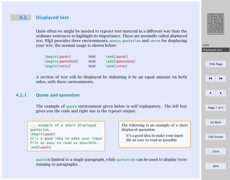
4.2. Displayed text
Quite often we might be needed to typeset text material in a different way than theordinary sentences to highlight its importance. These are normally called displayedtext. LATEX provides three environments, quote, quotation and verse for displayingyour text, the normal usage is shown below:
\beginquote text \endquote\beginquotation text \endquotation\beginverse text \endverse
A section of text will be displayed by indenting it by an equal amount on bothsides, with these environments.
4.2.1. Quote and quotation
The example of quote environment given below is self explanatory. The left boxgives you the code and right one is the typeset output.
... example of a short displayedquotation.\beginquoteIt’s a good idea to make your inputfile as easy to read as possible.\endquote
The following is an example of a shortdisplayed quotation.
It’s a good idea to make your inputfile as easy to read as possible.
quote is limited to a single paragraph, while quotation can be used to display textsrunning to paragraphs.
Lists
Displayed text
Title Page
ðð ññ
ð ñ
Page 8 of 8
Go Back
Full Screen
Close
Quit
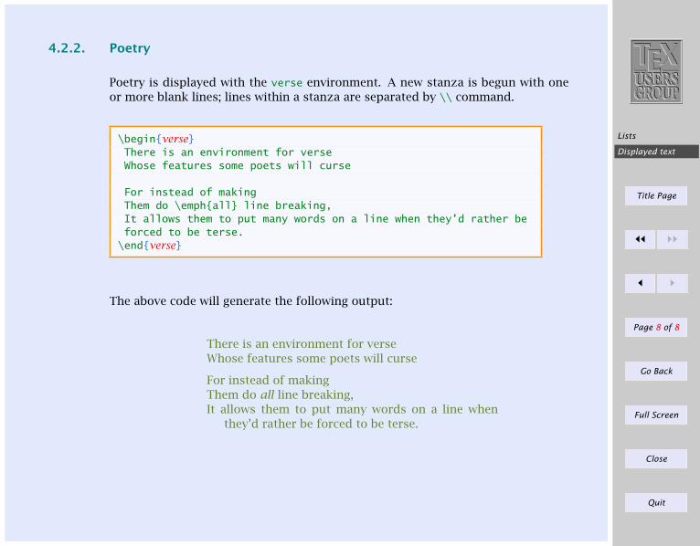
4.2.2. Poetry
Poetry is displayed with the verse environment. A new stanza is begun with oneor more blank lines; lines within a stanza are separated by \\ command.
\beginverseThere is an environment for verseWhose features some poets will curse
For instead of makingThem do \emphall line breaking,It allows them to put many words on a line when they’d rather beforced to be terse.
\endverse
The above code will generate the following output:
There is an environment for verseWhose features some poets will curse
For instead of makingThem do all line breaking,It allows them to put many words on a line when
they’d rather be forced to be terse.
LR Boxes
Paragraph Boxes
Paragraph . . .
Nested boxes
Rule boxes
Title Page
ðð ññ
ð ñ
Page 1 of 12
Go Back
Full Screen
Close
Quit
Indian TEX Users GroupURL: http://www.river-valley.com/tug
5On-line Tutorial on LATEX
The Tutorial TeamIndian TEX Users Group, SJP Buildings, Cotton Hills
Trivandrum 695014, INDIA2000
Prof. (Dr.) K. S. S. Nambooripad, Director, Center for Mathematical Sciences, Trivandrum, (Editor); Dr. E. Krishnan,Reader in Mathematics, University College, Trivandrum; T. Rishi, Focal Image (India) Pvt. Ltd., Trivandrum;L. A. Ajith, Focal Image (India) Pvt. Ltd., Trivandrum; A. M. Shan, Focal Image (India) Pvt. Ltd., Trivandrum;
C. V. Radhakrishnan, River Valley Technologies, Software Technology Park, Trivandrum constitute the Tutorial team
This document is generated from LATEX sources compiled with pdfLATEX v. 14e in anINTEL Pentium III 700 MHz system running Linux kernel version 2.2.14-12. The
packages used are hyperref.sty and pdfscreen.sty
c©2000, Indian TEX Users Group. This document may be distributed under the terms of theLATEX Project Public License, as described in lppl.txt in the base LATEX distribution, either
version 1.0 or, at your option, any later version
LR Boxes
Paragraph Boxes
Paragraph . . .
Nested boxes
Rule boxes
Title Page
ðð ññ
ð ñ
Page 2 of 12
Go Back
Full Screen
Close
Quit
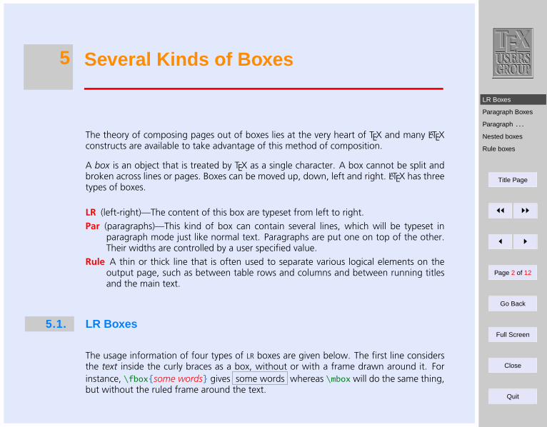
5 Several Kinds of Boxes
The theory of composing pages out of boxes lies at the very heart of TEX and many LATEXconstructs are available to take advantage of this method of composition.
A box is an object that is treated by TEX as a single character. A box cannot be split andbroken across lines or pages. Boxes can be moved up, down, left and right. LATEX has threetypes of boxes.
LR (left-right)—The content of this box are typeset from left to right.
Par (paragraphs)—This kind of box can contain several lines, which will be typeset inparagraph mode just like normal text. Paragraphs are put one on top of the other.Their widths are controlled by a user specified value.
Rule A thin or thick line that is often used to separate various logical elements on theoutput page, such as between table rows and columns and between running titlesand the main text.
5.1. LR Boxes
The usage information of four types of LR boxes are given below. The first line considersthe text inside the curly braces as a box, without or with a frame drawn around it. Forinstance, \fboxsome words gives some words whereas \mbox will do the same thing,but without the ruled frame around the text.
LR Boxes
Paragraph Boxes
Paragraph . . .
Nested boxes
Rule boxes
Title Page
ðð ññ
ð ñ
Page 3 of 12
Go Back
Full Screen
Close
Quit
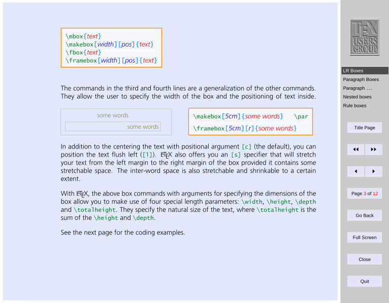
\mboxtext\makebox[width][pos]text\fboxtext\framebox[width][pos]text
The commands in the third and fourth lines are a generalization of the other commands.They allow the user to specify the width of the box and the positioning of text inside.
some words
some words
\makebox[5cm]some words \par
\framebox[5cm][r]some words
In addition to the centering the text with positional argument [c] (the default), you canposition the text flush left ([l]). LATEX also offers you an [s] specifier that will stretchyour text from the left margin to the right margin of the box provided it contains somestretchable space. The inter-word space is also stretchable and shrinkable to a certainextent.
With LATEX, the above box commands with arguments for specifying the dimensions of thebox allow you to make use of four special length parameters: \width, \height, \depthand \totalheight. They specify the natural size of the text, where \totalheight is thesum of the \height and \depth.
See the next page for the coding examples.
LR Boxes
Paragraph Boxes
Paragraph . . .
Nested boxes
Rule boxes
Title Page
ðð ññ
ð ñ
Page 4 of 12
Go Back
Full Screen
Close
Quit
A few words of advice
A few words of advice
A few words of advice
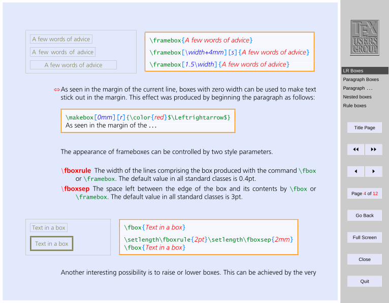
\frameboxA few words of advice
\framebox[\width+4mm][s]A few words of advice
\framebox[1.5\width]A few words of advice
aAs seen in the margin of the current line, boxes with zero width can be used to make textstick out in the margin. This effect was produced by beginning the paragraph as follows:
\makebox[0mm][r]\colorred$\Leftrightarrow$As seen in the margin of the . . .
The appearance of frameboxes can be controlled by two style parameters.
\fboxrule The width of the lines comprising the box produced with the command \fboxor \framebox. The default value in all standard classes is 0.4pt.
\fboxsep The space left between the edge of the box and its contents by \fbox or\framebox. The default value in all standard classes is 3pt.
Text in a box
Text in a box
\fboxText in a box
\setlength\fboxrule2pt\setlength\fboxsep2mm\fboxText in a box
Another interesting possibility is to raise or lower boxes. This can be achieved by the very
LR Boxes
Paragraph Boxes
Paragraph . . .
Nested boxes
Rule boxes
Title Page
ðð ññ
ð ñ
Page 5 of 12
Go Back
Full Screen
Close
Quit
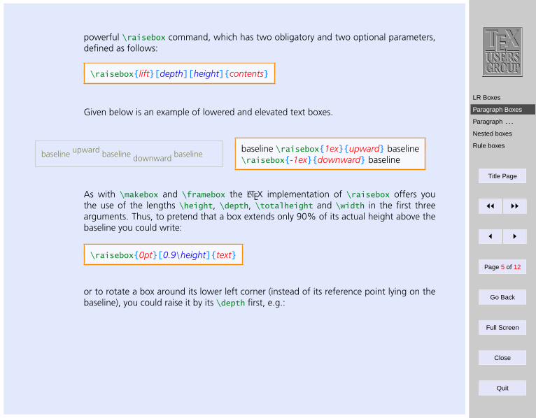
powerful \raisebox command, which has two obligatory and two optional parameters,defined as follows:
\raiseboxlift[depth][height]contents
Given below is an example of lowered and elevated text boxes.
baseline upward baseline downward baselinebaseline \raisebox1exupward baseline\raisebox-1exdownward baseline
As with \makebox and \framebox the LATEX implementation of \raisebox offers youthe use of the lengths \height, \depth, \totalheight and \width in the first threearguments. Thus, to pretend that a box extends only 90% of its actual height above thebaseline you could write:
\raisebox0pt[0.9\height]text
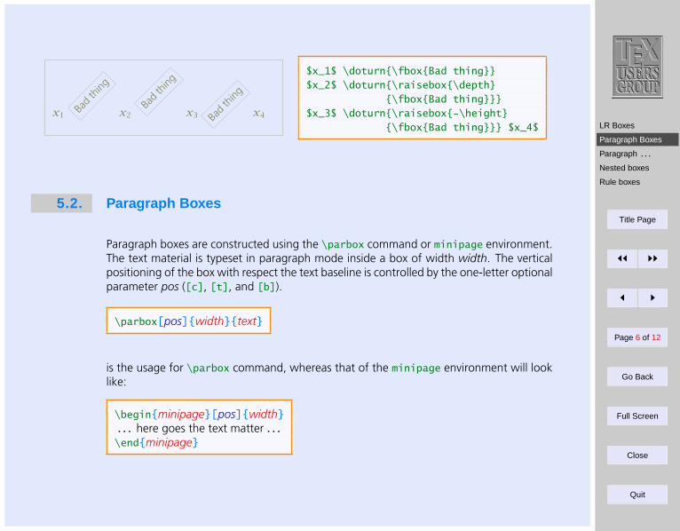
or to rotate a box around its lower left corner (instead of its reference point lying on thebaseline), you could raise it by its \depth first, e.g.:
LR Boxes
Paragraph Boxes
Paragraph . . .
Nested boxes
Rule boxes
Title Page
ðð ññ
ð ñ
Page 6 of 12
Go Back
Full Screen
Close
Quit
x1 Bad
thing
x2Ba
dth
ing
x3 Bad
thing
x4
$x_1$ \doturn\fboxBad thing$x_2$ \doturn\raisebox\depth
\fboxBad thing$x_3$ \doturn\raisebox-\height
\fboxBad thing $x_4$
5.2. Paragraph Boxes
Paragraph boxes are constructed using the \parbox command or minipage environment.The text material is typeset in paragraph mode inside a box of width width. The verticalpositioning of the box with respect the text baseline is controlled by the one-letter optionalparameter pos ([c], [t], and [b]).
\parbox[pos]widthtext
is the usage for \parbox command, whereas that of the minipage environment will looklike:
\beginminipage[pos]width. . . here goes the text matter . . .\endminipage
LR Boxes
Paragraph Boxes
Paragraph . . .
Nested boxes
Rule boxes
Title Page
ðð ññ
ð ñ
Page 7 of 12
Go Back
Full Screen
Close
Quit
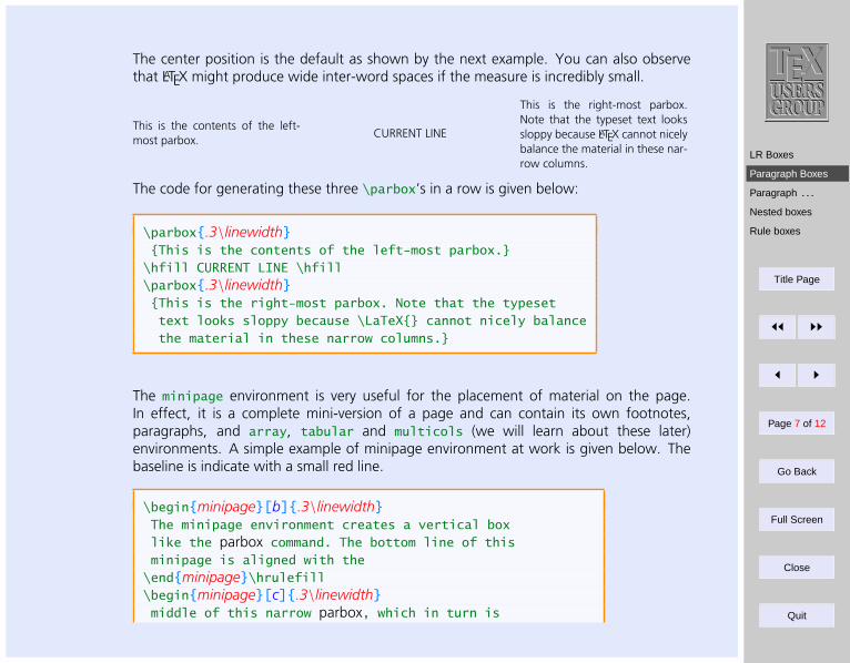
The center position is the default as shown by the next example. You can also observethat LATEX might produce wide inter-word spaces if the measure is incredibly small.
This is the contents of the left-most parbox.
CURRENT LINE
This is the right-most parbox.Note that the typeset text lookssloppy because LATEX cannot nicelybalance the material in these nar-row columns.
The code for generating these three \parbox’s in a row is given below:
\parbox.3\linewidthThis is the contents of the left-most parbox.
\hfill CURRENT LINE \hfill\parbox.3\linewidthThis is the right-most parbox. Note that the typesettext looks sloppy because \LaTeX cannot nicely balancethe material in these narrow columns.
The minipage environment is very useful for the placement of material on the page.In effect, it is a complete mini-version of a page and can contain its own footnotes,paragraphs, and array, tabular and multicols (we will learn about these later)environments. A simple example of minipage environment at work is given below. Thebaseline is indicate with a small red line.
\beginminipage[b].3\linewidthThe minipage environment creates a vertical boxlike the parbox command. The bottom line of thisminipage is aligned with the
\endminipage\hrulefill\beginminipage[c].3\linewidthmiddle of this narrow parbox, which in turn is
LR Boxes
Paragraph Boxes
Paragraph . . .
Nested boxes
Rule boxes
Title Page
ðð ññ
ð ñ
Page 8 of 12
Go Back
Full Screen
Close
Quit
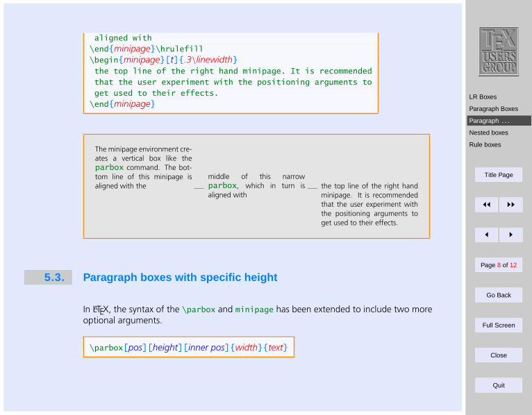
aligned with\endminipage\hrulefill\beginminipage[t].3\linewidththe top line of the right hand minipage. It is recommendedthat the user experiment with the positioning arguments toget used to their effects.
\endminipage
The minipage environment cre-ates a vertical box like theparbox command. The bot-tom line of this minipage isaligned with the
middle of this narrowparbox, which in turn isaligned with
the top line of the right handminipage. It is recommendedthat the user experiment withthe positioning arguments toget used to their effects.
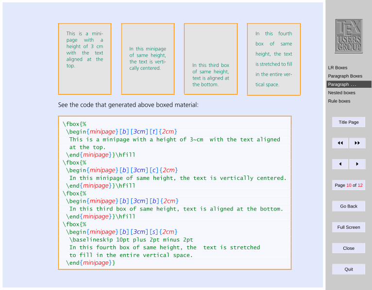
5.3. Paragraph boxes with specific height
In LATEX, the syntax of the \parbox and minipage has been extended to include two moreoptional arguments.
\parbox[pos][height][inner pos]widthtext
LR Boxes
Paragraph Boxes
Paragraph . . .
Nested boxes
Rule boxes
Title Page
ðð ññ
ð ñ
Page 9 of 12
Go Back
Full Screen
Close
Quit
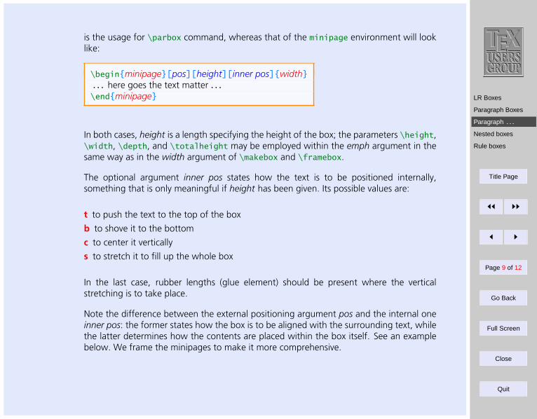
is the usage for \parbox command, whereas that of the minipage environment will looklike:
\beginminipage[pos][height][inner pos]width. . . here goes the text matter . . .\endminipage
In both cases, height is a length specifying the height of the box; the parameters \height,\width, \depth, and \totalheight may be employed within the emph argument in thesame way as in the width argument of \makebox and \framebox.
The optional argument inner pos states how the text is to be positioned internally,something that is only meaningful if height has been given. Its possible values are:
t to push the text to the top of the box
b to shove it to the bottom
c to center it vertically
s to stretch it to fill up the whole box
In the last case, rubber lengths (glue element) should be present where the verticalstretching is to take place.
Note the difference between the external positioning argument pos and the internal oneinner pos: the former states how the box is to be aligned with the surrounding text, whilethe latter determines how the contents are placed within the box itself. See an examplebelow. We frame the minipages to make it more comprehensive.
LR Boxes
Paragraph Boxes
Paragraph . . .
Nested boxes
Rule boxes
Title Page
ðð ññ
ð ñ
Page 10 of 12
Go Back
Full Screen
Close
Quit
This is a mini-page with aheight of 3 cmwith the textaligned at thetop.
In this minipageof same height,the text is verti-cally centered. In this third box
of same height,text is aligned atthe bottom.
In this fourth
box of same
height, the text
is stretched to fill
in the entire ver-
tical space.
See the code that generated above boxed material:
\fbox%\beginminipage[b][3cm][t]2cmThis is a minipage with a height of 3~cm with the text alignedat the top.\endminipage\hfill
\fbox%\beginminipage[b][3cm][c]2cmIn this minipage of same height, the text is vertically centered.\endminipage\hfill
\fbox%\beginminipage[b][3cm][b]2cmIn this third box of same height, text is aligned at the bottom.\endminipage\hfill
\fbox%\beginminipage[b][3cm][s]2cm\baselineskip 10pt plus 2pt minus 2ptIn this fourth box of same height, the text is stretchedto fill in the entire vertical space.\endminipage
LR Boxes
Paragraph Boxes
Paragraph . . .
Nested boxes
Rule boxes
Title Page
ðð ññ
ð ñ
Page 11 of 12
Go Back
Full Screen
Close
Quit
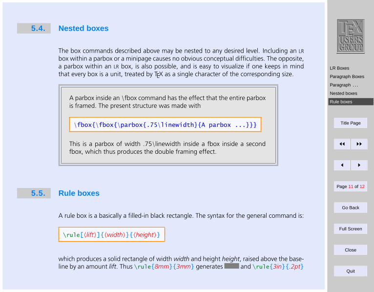
5.4. Nested boxes
The box commands described above may be nested to any desired level. Including an LR
box within a parbox or a minipage causes no obvious conceptual difficulties. The opposite,a parbox within an LR box, is also possible, and is easy to visualize if one keeps in mindthat every box is a unit, treated by TEX as a single character of the corresponding size.
A parbox inside an \fbox command has the effect that the entire parboxis framed. The present structure was made with
\fbox\fbox\parbox.75\linewidthA parbox ...
This is a parbox of width .75\linewidth inside a fbox inside a secondfbox, which thus produces the double framing effect.
5.5. Rule boxes
A rule box is a basically a filled-in black rectangle. The syntax for the general command is:
\rule[〈lift〉]〈width〉〈height〉
which produces a solid rectangle of width width and height height, raised above the base-line by an amount lift. Thus \rule8mm3mm generates and \rule3in.2pt
LR Boxes
Paragraph Boxes
Paragraph . . .
Nested boxes
Rule boxes
Title Page
ðð ññ
ð ñ
Page 12 of 12
Go Back
Full Screen
Close
Quit
generates .
Without an optional argument lift, the rectangle is set on the baseline of the current lineof the text. The parameters lift, width and height are all lengths. If lift has a negativevalue, the rectangle is set below the baseline.
It is also possible to have a rule box of zero width. This creates an invisible line with thegiven height. Such a construction is called a strut and is used to force a horizontal box tohave a desired height or depth that is different from that of its contents.
Table
Table style pa . . .
Example
Exercise
Title Page
ðð ññ
ð ñ
Page 1 of 8
Go Back
Full Screen
Close
Quit
Indian TEX Users GroupURL: http://www.river-valley.com/tug
6On-line Tutorial on LATEX
The Tutorial TeamIndian TEX Users Group, SJP Buildings, Cotton Hills
Trivandrum 695014, INDIA2000
Prof. (Dr.) K. S. S. Nambooripad, Director, Center for Mathematical Sciences, Trivandrum, (Editor); Dr. E. Krishnan,Reader in Mathematics, University College, Trivandrum; T. Rishi, Focal Image (India) Pvt. Ltd., Trivandrum;L. A. Ajith, Focal Image (India) Pvt. Ltd., Trivandrum; A. M. Shan, Focal Image (India) Pvt. Ltd., Trivandrum;
C. V. Radhakrishnan, River Valley Technologies, Software Technology Park, Trivandrum constitute the Tutorial team
This document is generated from LATEX sources compiled with pdfLATEX v. 14e in anINTEL Pentium III 700 MHz system running Linux kernel version 2.2.14-12. The
packages used are hyperref.sty and pdfscreen.sty
c©2000, Indian TEX Users Group. This document may be distributed under the terms of theLATEX Project Public License, as described in lppl.txt in the base LATEX distribution, either
version 1.0 or, at your option, any later version
Table
Table style pa . . .
Example
Exercise
Title Page
ðð ññ
ð ñ
Page 2 of 8
Go Back
Full Screen
Close
Quit
6 Floats
6.1. Table
With the box elements already explained in the previous chapter, it would be possible toproduce all sorts of framed and unframed tables. However, LATEX offers the user far moreconvenient ways to build such complicated structures.
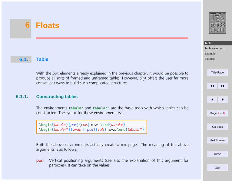
6.1.1. Constructing tables
The environments tabular and tabular* are the basic tools with which tables can beconstructed. The syntax for these environments is:
\begintabular[pos]cols rows \endtabular\begintabular*width[pos]cols rows \endtabular*
Both the above environments actually create a minipage. The meaning of the abovearguments is as follows:
pos Vertical positioning arguments (see also the explanation of this argument forparboxes). It can take on the values.
Table
Table style pa . . .
Example
Exercise
Title Page
ðð ññ
ð ñ
Page 3 of 8
Go Back
Full Screen
Close
Quit
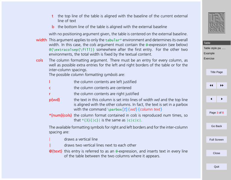
t the top line of the table is aligned with the baseline of the current externalline of text
b the bottom line of the table is aligned with the external baseline
with no positioning argument given, the table is centered on the external baseline.
width This argument applies to only the tabular* environment and determines its overallwidth. In this case, the cols argument must contain the @-expression (see below)@\extracolsep\fill somewhere after the first entry. For the other twoenvironments, the total width is fixed by the textual content.
cols The column formatting argument. There must be an entry for every column, aswell as possible extra entries for the left and right borders of the table or for theinter-column spacings.The possible column formatting symbols are:
l the column contents are left justified
c the column contents are centered
r the column contents are right justified
pwd the text in this column is set into lines of width wd and the top lineis aligned with the other columns. In fact, the text is set in a parboxwith the command \parbox[t]wdcolumn text
*numcols the column format contained in cols is reproduced num times, sothat *3|c| is the same as |c|c|c|.
The available formatting symbols for right and left borders and for the inter-columnspacing are:
| draws a vertical line
‖ draws two vertical lines next to each other
@text this entry is referred to as an @-expression, and inserts text in every lineof the table between the two columns where it appears.
Table
Table style pa . . .
Example
Exercise
Title Page
ðð ññ
ð ñ
Page 4 of 8
Go Back
Full Screen
Close
Quit
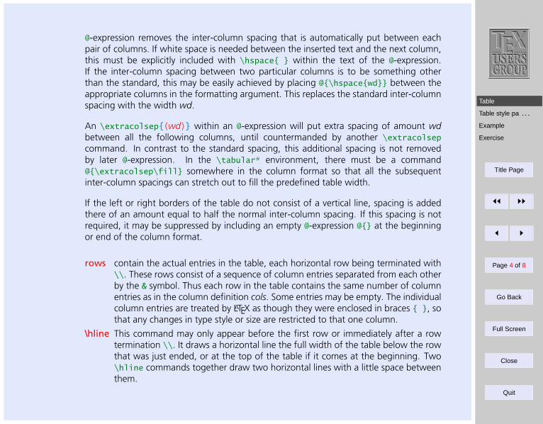
@-expression removes the inter-column spacing that is automatically put between eachpair of columns. If white space is needed between the inserted text and the next column,this must be explicitly included with \hspace within the text of the @-expression.If the inter-column spacing between two particular columns is to be something otherthan the standard, this may be easily achieved by placing @\hspacewd between theappropriate columns in the formatting argument. This replaces the standard inter-columnspacing with the width wd.
An \extracolsep〈wd〉 within an @-expression will put extra spacing of amount wdbetween all the following columns, until countermanded by another \extracolsepcommand. In contrast to the standard spacing, this additional spacing is not removedby later @-expression. In the \tabular* environment, there must be a command@\extracolsep\fill somewhere in the column format so that all the subsequentinter-column spacings can stretch out to fill the predefined table width.
If the left or right borders of the table do not consist of a vertical line, spacing is addedthere of an amount equal to half the normal inter-column spacing. If this spacing is notrequired, it may be suppressed by including an empty @-expression @ at the beginningor end of the column format.
rows contain the actual entries in the table, each horizontal row being terminated with\\. These rows consist of a sequence of column entries separated from each otherby the & symbol. Thus each row in the table contains the same number of columnentries as in the column definition cols. Some entries may be empty. The individualcolumn entries are treated by LATEX as though they were enclosed in braces , sothat any changes in type style or size are restricted to that one column.
\hline This command may only appear before the first row or immediately after a rowtermination \\. It draws a horizontal line the full width of the table below the rowthat was just ended, or at the top of the table if it comes at the beginning. Two\hline commands together draw two horizontal lines with a little space betweenthem.
Table
Table style pa . . .
Example
Exercise
Title Page
ðð ññ
ð ñ
Page 5 of 8
Go Back
Full Screen
Close
Quit
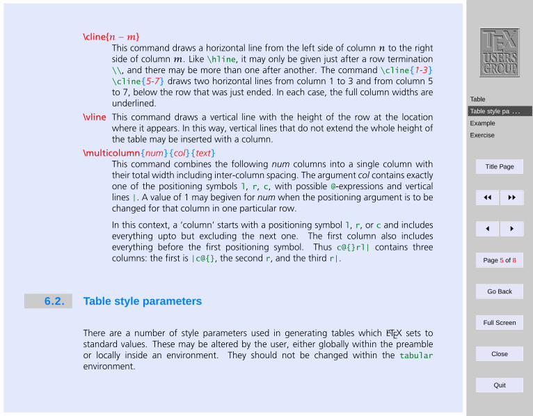
\clinen−mThis command draws a horizontal line from the left side of column n to the rightside of column m. Like \hline, it may only be given just after a row termination\\, and there may be more than one after another. The command \cline1-3\cline5-7 draws two horizontal lines from column 1 to 3 and from column 5to 7, below the row that was just ended. In each case, the full column widths areunderlined.
\vline This command draws a vertical line with the height of the row at the locationwhere it appears. In this way, vertical lines that do not extend the whole height ofthe table may be inserted with a column.
\multicolumnnumcoltextThis command combines the following num columns into a single column withtheir total width including inter-column spacing. The argument col contains exactlyone of the positioning symbols l, r, c, with possible @-expressions and verticallines |. A value of 1 may begiven for num when the positioning argument is to bechanged for that column in one particular row.
In this context, a ‘column’ starts with a positioning symbol l, r, or c and includeseverything upto but excluding the next one. The first column also includeseverything before the first positioning symbol. Thus c@rl| contains threecolumns: the first is |c@, the second r, and the third r|.
6.2. Table style parameters
There are a number of style parameters used in generating tables which LATEX sets tostandard values. These may be altered by the user, either globally within the preambleor locally inside an environment. They should not be changed within the tabularenvironment.
Table
Table style pa . . .
Example
Exercise
Title Page
ðð ññ
ð ñ
Page 6 of 8
Go Back
Full Screen
Close
Quit
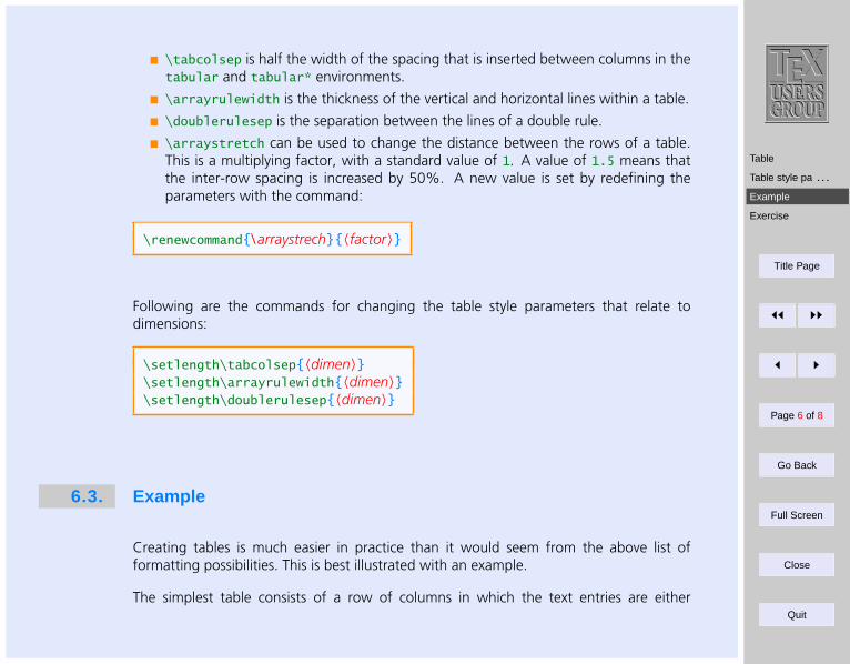
\tabcolsep is half the width of the spacing that is inserted between columns in thetabular and tabular* environments.
\arrayrulewidth is the thickness of the vertical and horizontal lines within a table.
\doublerulesep is the separation between the lines of a double rule.
\arraystretch can be used to change the distance between the rows of a table.This is a multiplying factor, with a standard value of 1. A value of 1.5 means thatthe inter-row spacing is increased by 50%. A new value is set by redefining theparameters with the command:
\renewcommand\ arraystrech〈factor〉
Following are the commands for changing the table style parameters that relate todimensions:
\setlength\tabcolsep〈dimen〉\setlength\arrayrulewidth〈dimen〉\setlength\doublerulesep〈dimen〉
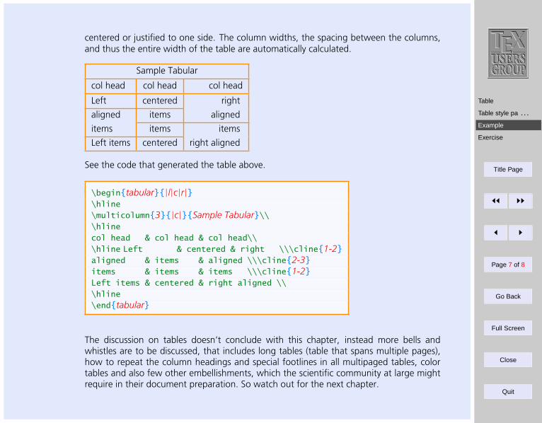
6.3. Example
Creating tables is much easier in practice than it would seem from the above list offormatting possibilities. This is best illustrated with an example.
The simplest table consists of a row of columns in which the text entries are either
Table
Table style pa . . .
Example
Exercise
Title Page
ðð ññ
ð ñ
Page 7 of 8
Go Back
Full Screen
Close
Quit
centered or justified to one side. The column widths, the spacing between the columns,and thus the entire width of the table are automatically calculated.
Sample Tabular
col head col head col head
Left centered right
aligned items aligned
items items items
Left items centered right aligned
See the code that generated the table above.
\begintabular|l|c|r|\hline\multicolumn3|c|Sample Tabular\\\hlinecol head & col head & col head\\\hline Left & centered & right \\\cline1-2aligned & items & aligned \\\cline2-3items & items & items \\\cline1-2Left items & centered & right aligned \\\hline\endtabular
The discussion on tables doesn’t conclude with this chapter, instead more bells andwhistles are to be discussed, that includes long tables (table that spans multiple pages),how to repeat the column headings and special footlines in all multipaged tables, colortables and also few other embellishments, which the scientific community at large mightrequire in their document preparation. So watch out for the next chapter.
Table
Table style pa . . .
Example
Exercise
Title Page
ðð ññ
ð ñ
Page 8 of 8
Go Back
Full Screen
Close
Quit
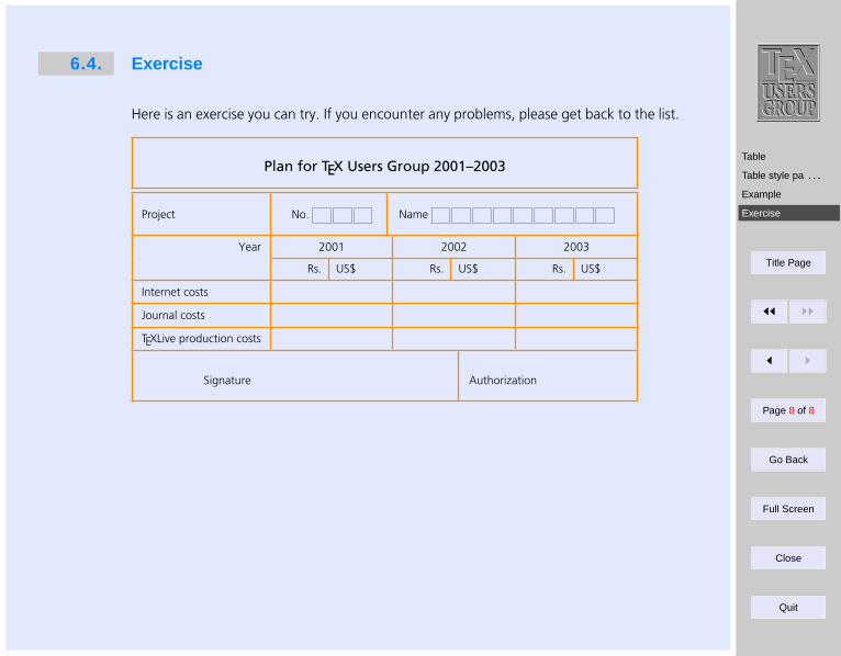
6.4. Exercise
Here is an exercise you can try. If you encounter any problems, please get back to the list.
Plan for TEX Users Group 2001–2003
Project No. Name
Year 2001 2002 2003
Rs. US$ Rs. US$ Rs. US$
Internet costs
Journal costs
TEXLive production costs
Signature Authorization
Longtable
Another example
Exercise
Title Page
JJ II
J I
Page 1 of 10
Go Back
Full Screen
Close
Quit
Indian TEX Users GroupURL: http://www.river-valley.com/tug
7On-line Tutorial on LATEX
The Tutorial TeamIndian TEX Users Group,SJPBuildings, Cotton Hills
Trivandrum695014, INDIA2000
Prof. (Dr.) K. S. S. Nambooripad, Director, Center for Mathematical Sciences, Trivandrum, (Editor); Dr. E. Krishnan,Reader in Mathematics, University College, Trivandrum; Mohit Agarwal, Department of Aerospace Engineering,
Indian Institute of Science, Bangalore; T. Rishi, Focal Image (India) Pvt. Ltd., Trivandrum; L. A. Ajith, Focal Image(India) Pvt. Ltd., Trivandrum; A. M. Shan, Focal Image (India) Pvt. Ltd., Trivandrum; C. V. Radhakrishnan, River
Valley Technologies, Software Technology Park, Trivandrum constitute the Tutorial team
This document is generated from LATEX sources compiled with pdfLATEX v. 14e in anINTEL Pentium III 700 MHz system running Linux kernel version 2.2.14-12. The
packages used are hyperref.sty and pdfscreen.sty
c©2000, Indian TEX Users Group. This document may be distributed under the terms of theLATEX Project Public License, as described in lppl.txt in the base LATEX distribution, either
version 1.0 or, at your option, any later version
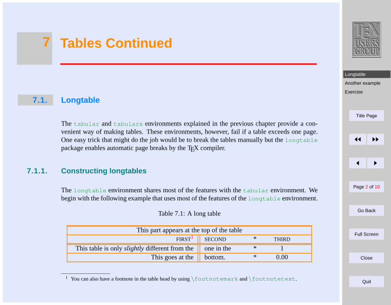
Longtable
Another example
Exercise
Title Page
JJ II
J I
Page 2 of 10
Go Back
Full Screen
Close
Quit
7 Tables Continued
7.1. Longtable
The tabular and tabularx environments explained in the previous chapter provide a con-venient way of making tables. These environments, however, fail if a table exceeds one page.One easy trick that might do the job would be to break the tables manually but thelongtable
package enables automatic page breaks by the TEX compiler.
7.1.1. Constructing longtables
The longtable environment shares most of the features with thetabular environment. Webegin with the following example that uses most of the features of thelongtable environment.
Table 7.1: A long table
This part appears at the top of the tableFIRST1 SECOND * THIRD
This table is onlyslightlydifferent from the one in the * 1This goes at the bottom. * 0.00
1 You can also have a footnote in the table head by using\footnotemark and\footnotetext .
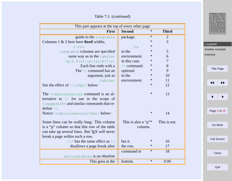
Longtable
Another example
Exercise
Title Page
JJ II
J I
Page 3 of 10
Go Back
Full Screen
Close
Quit
Table 7.1: (continued)
This part appears at the top of every other pageFirst Second * Third
guide to thelongtable package. * 2Columns 1 & 2 here havefixed widths. * 3
2.5in 1in *longtable columns are specified in the * 5
same way as in thetabular environment. * 6|p2.5in||p1in@*c| in this case. * 7
Each line ends with a \\ command. * 8The \\ command has an optional * 9
argument, just as in the * 10tabular environment. * 11
See the effect of\\[10pt] below: * 12
The \tabularnewline command is an al-ternative to \\ for use in the scope of\raggedleft and similar commands that re-define\\ .
* 13
Notice \tabularnewline[10pt] below: * 14
Some lines can be really long: This columnis a “p” column so that this row of the tablecan take up several lines. But TEX will neverbreak a page within such a row.
This is also a “p”column.
* This is not.
\\* has the same effect as\\ but it * 16disallows a page break after the row. * 17
setlongtables is an obsoletecommand in * 18
This goes at the bottom. * 0.00
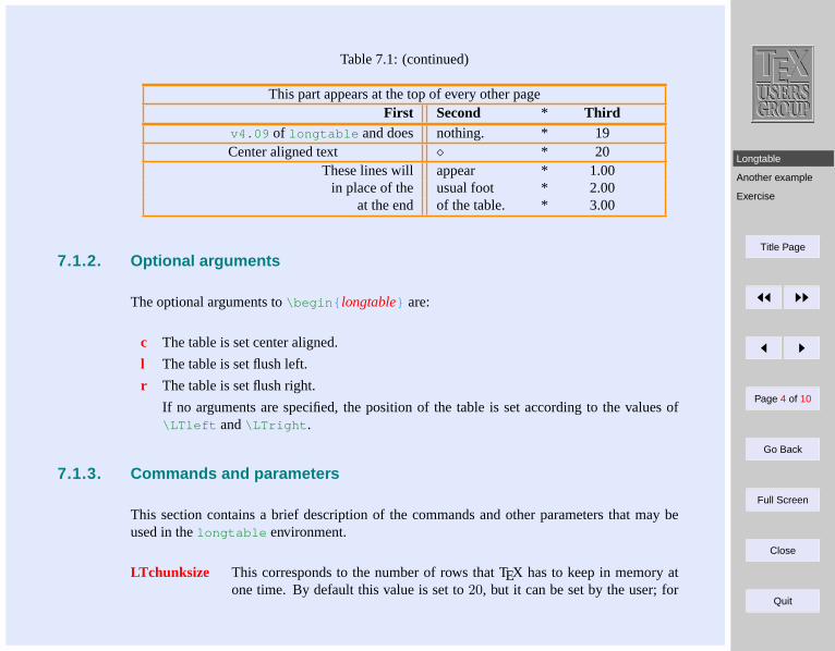
Longtable
Another example
Exercise
Title Page
JJ II
J I
Page 4 of 10
Go Back
Full Screen
Close
Quit
Table 7.1: (continued)
This part appears at the top of every other pageFirst Second * Third
v4.09 of longtable and does nothing. * 19Center aligned text * 20
These lines will appear * 1.00in place of the usual foot * 2.00
at the end of the table. * 3.00
7.1.2. Optional arguments
The optional arguments to\begin longtable are:
c The table is set center aligned.
l The table is set flush left.
r The table is set flush right.
If no arguments are specified, the position of the table is set according to the values of\LTleft and\LTright .
7.1.3. Commands and parameters
This section contains a brief description of the commands and other parameters that may beused in thelongtable environment.
LTchunksize This corresponds to the number of rows that TEX has to keep in memory atone time. By default this value is set to20, but it can be set by the user; for
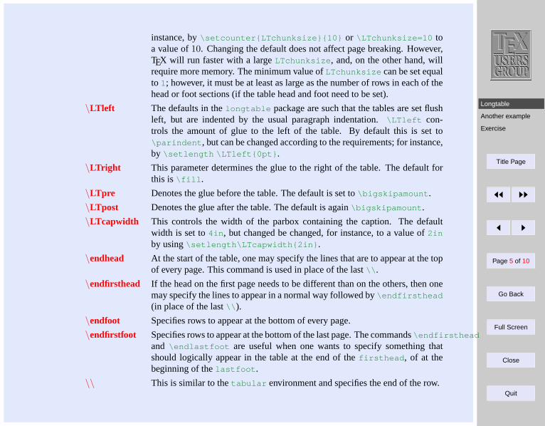
Longtable
Another example
Exercise
Title Page
JJ II
J I
Page 5 of 10
Go Back
Full Screen
Close
Quit
instance, by\setcounterLTchunksize10 or \LTchunksize=10 toa value of10. Changing the default does not affect page breaking. However,TEX will run faster with a largeLTchunksize , and, on the other hand, willrequire more memory. The minimum value ofLTchunksize can be set equalto 1; however, it must be at least as large as the number of rows in each of thehead or foot sections (if the table head and foot need to be set).
\LTleft The defaults in thelongtable package are such that the tables are set flushleft, but are indented by the usual paragraph indentation.\LTleft con-trols the amount of glue to the left of the table. By default this is set to\parindent , but can be changed according to the requirements; for instance,by \setlength \LTleft0pt .
\LTright This parameter determines the glue to the right of the table. The default forthis is \fill .
\LTpre Denotes the glue before the table. The default is set to\bigskipamount .
\LTpost Denotes the glue after the table. The default is again\bigskipamount .
\LTcapwidth This controls the width of the parbox containing the caption. The defaultwidth is set to4in , but changed be changed, for instance, to a value of2in
by using\setlength\LTcapwidth2in .
\endhead At the start of the table, one may specify the lines that are to appear at the topof every page. This command is used in place of the last\\ .
\endfirsthead If the head on the first page needs to be different than on the others, then onemay specify the lines to appear in a normal way followed by\endfirsthead
(in place of the last\\ ).
\endfoot Specifies rows to appear at the bottom of every page.
\endfirstfoot Specifies rows to appear at the bottom of the last page. The commands\endfirsthead
and \endlastfoot are useful when one wants to specify something thatshould logically appear in the table at the end of thefirsthead , of at thebeginning of thelastfoot .
\\ This is similar to thetabular environment and specifies the end of the row.
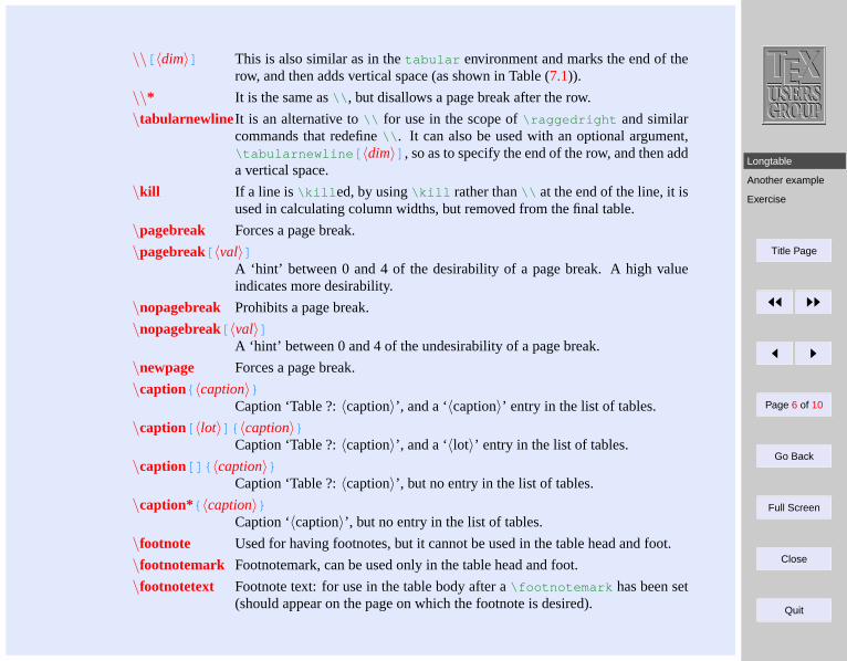
Longtable
Another example
Exercise
Title Page
JJ II
J I
Page 6 of 10
Go Back
Full Screen
Close
Quit
\\[ 〈dim〉] This is also similar as in thetabular environment and marks the end of therow, and then adds vertical space (as shown in Table (7.1)).
\\* It is the same as\\ , but disallows a page break after the row.
\tabularnewline It is an alternative to\\ for use in the scope of\raggedright and similarcommands that redefine\\ . It can also be used with an optional argument,\tabularnewline [ 〈dim〉] , so as to specify the end of the row, and then adda vertical space.
\kill If a line is \kill ed, by using\kill rather than\\ at the end of the line, it isused in calculating column widths, but removed from the final table.
\pagebreak Forces a page break.
\pagebreak[ 〈val〉]A ‘hint’ between 0 and 4 of the desirability of a page break. A high valueindicates more desirability.
\nopagebreak Prohibits a page break.
\nopagebreak[ 〈val〉]A ‘hint’ between 0 and 4 of the undesirability of a page break.
\newpage Forces a page break.
\caption 〈caption〉Caption ‘Table ?:〈caption〉’, and a ‘〈caption〉’ entry in the list of tables.
\caption[ 〈lot〉] 〈caption〉Caption ‘Table ?:〈caption〉’, and a ‘〈lot〉’ entry in the list of tables.
\caption[ ] 〈caption〉Caption ‘Table ?:〈caption〉’, but no entry in the list of tables.
\caption* 〈caption〉Caption ‘〈caption〉’, but no entry in the list of tables.
\footnote Used for having footnotes, but it cannot be used in the table head and foot.
\footnotemark Footnotemark, can be used only in the table head and foot.
\footnotetext Footnote text: for use in the table body after a\footnotemark has been set(should appear on the page on which the footnote is desired).
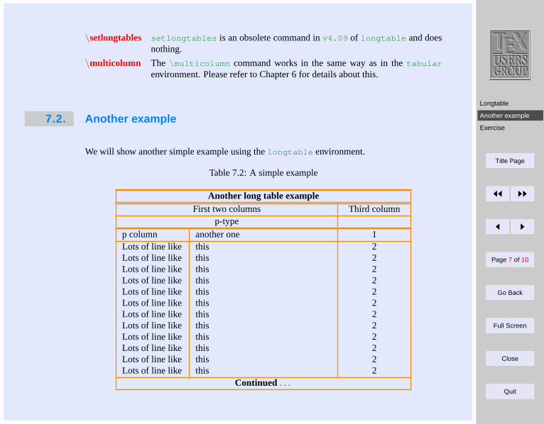
Longtable
Another example
Exercise
Title Page
JJ II
J I
Page 7 of 10
Go Back
Full Screen
Close
Quit
\setlongtables setlongtables is an obsolete command inv4.09 of longtable and doesnothing.
\multicolumn The \multicolumn command works in the same way as in thetabular
environment. Please refer to Chapter 6 for details about this.
7.2. Another example
We will show another simple example using thelongtable environment.
Table 7.2: A simple example
Another long table exampleFirst two columns Third column
p-type
p column another one 1Lots of line like this 2Lots of line like this 2Lots of line like this 2Lots of line like this 2Lots of line like this 2Lots of line like this 2Lots of line like this 2Lots of line like this 2Lots of line like this 2Lots of line like this 2Lots of line like this 2Lots of line like this 2
Continued . . .
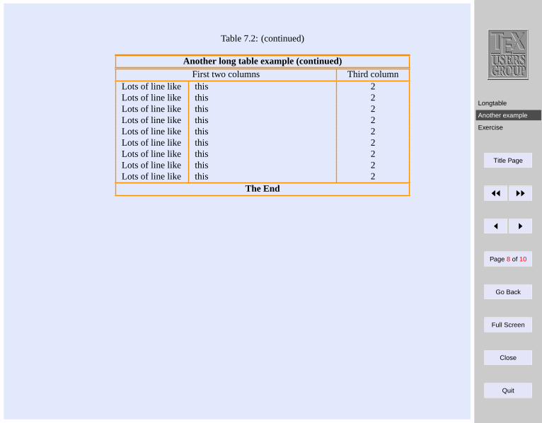
Longtable
Another example
Exercise
Title Page
JJ II
J I
Page 8 of 10
Go Back
Full Screen
Close
Quit
Table 7.2: (continued)
Another long table example (continued)First two columns Third column
Lots of line like this 2Lots of line like this 2Lots of line like this 2Lots of line like this 2Lots of line like this 2Lots of line like this 2Lots of line like this 2Lots of line like this 2Lots of line like this 2
The End
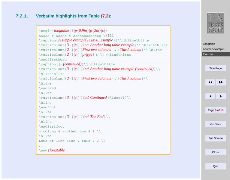
Longtable
Another example
Exercise
Title Page
JJ II
J I
Page 9 of 10
Go Back
Full Screen
Close
Quit
7.2.1. Verbatim highlights from Table ( 7.2):
\begin longtable |p0.9in|p2in|c|xxxxx & xxxxx & xxxxxxxxxxxxx \kill
\caption A simple example\label simple \\ \hline\hline
\multicolumn 3 |c| \bf Another long table example \\ \hline\hline
\multicolumn 2 |c| First two columns & Third column \\ \hline
\multicolumn 2 |c| p-type & \\ \hline\hline
\endfirsthead
\caption [ ] (continued) \\ \hline\hline
\multicolumn 3 |c| \bf Another long table example (continued) \\
\hline\hline
\multicolumn 2 |c| First two columns & Third column \\
\hline
\endhead
\hline
\multicolumn 3 |c| \bf Continued$\ldots$ \\
\hline
\endfoot
\hline
\multicolumn 3 |c| \bf The End \\
\hline
\endlastfoot
p column & another one & 1 \\
\hline
Lots of line like & this & 2 \\
. . .\end longtable
Longtable
Another example
Exercise
Title Page
JJ II
J I
Page 10 of 10
Go Back
Full Screen
Close
Quit
7.3. Exercise
Try making Table (7.1); it seems to be quite strange, but it contains most of the features onewould need in order to get thoroughly acquainted with thelongtable environment. It shouldbequite easyif one actually reads the table itself. Look at the spacescarefully.
The \colortbl . . .
More colors and . . .
Color tables . . .
More Examples . . .
Title Page
ðð ññ
ð ñ
Page 1 of 14
Go Back
Full Screen
Close
Quit
Indian TEX Users GroupURL: http://www.river-valley.com/tug
8On-line Tutorial on LATEX
The Tutorial TeamIndian TEX Users Group,SJPBuildings, Cotton Hills
Trivandrum 695014,INDIA
2000
Prof. (Dr.) K. S. S. Nambooripad, Director, Center for Mathematical Sciences, Trivandrum, (Editor); Dr. E. Krishnan,Reader in Mathematics, University College, Trivandrum; Mohit Agarwal, Department of Aerospace Engineering,
Indian Institute of Science, Bangalore; T. Rishi, Focal Image (India) Pvt. Ltd., Trivandrum; L. A. Ajith, Focal Image(India) Pvt. Ltd., Trivandrum; A. M. Shan, Focal Image (India) Pvt. Ltd., Trivandrum; C. V. Radhakrishnan, River
Valley Technologies, Software Technology Park, Trivandrum constitute the Tutorial team
This document is generated from LATEX sources compiled with pdfLATEX v. 14e in anINTEL Pentium III 700 MHz system running Linux kernel version 2.2.14-12. The
packages used are hyperref.sty and pdfscreen.sty
c©2000, Indian TEX Users Group. This document may be distributed under the terms of theLATEX Project Public License, as described in lppl.txt in the base LATEX distribution, either
version 1.0 or, at your option, any later version
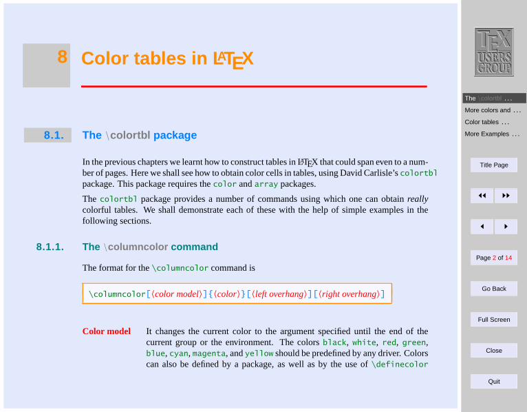
The \colortbl . . .
More colors and . . .
Color tables . . .
More Examples . . .
Title Page
ðð ññ
ð ñ
Page 2 of 14
Go Back
Full Screen
Close
Quit
8 Color tables in L ATEX
8.1. The \colortbl package
In the previous chapters we learnt how to construct tables in LATEX that could span even to a num-ber of pages. Here we shall see how to obtain color cells in tables, using David Carlisle’scolortblpackage. This package requires thecolor andarray packages.
The colortbl package provides a number of commands using which one can obtainreallycolorful tables. We shall demonstrate each of these with the help of simple examples in thefollowing sections.
8.1.1. The \columncolor command
The format for the\columncolor command is
\columncolor[〈color model〉]〈color〉[〈left overhang〉][〈right overhang〉]
Color model It changes the current color to the argument specified until the end of thecurrent group or the environment. The colorsblack, white, red, green,blue, cyan, magenta, andyellow should be predefined by any driver. Colorscan also be defined by a package, as well as by the use of\definecolor
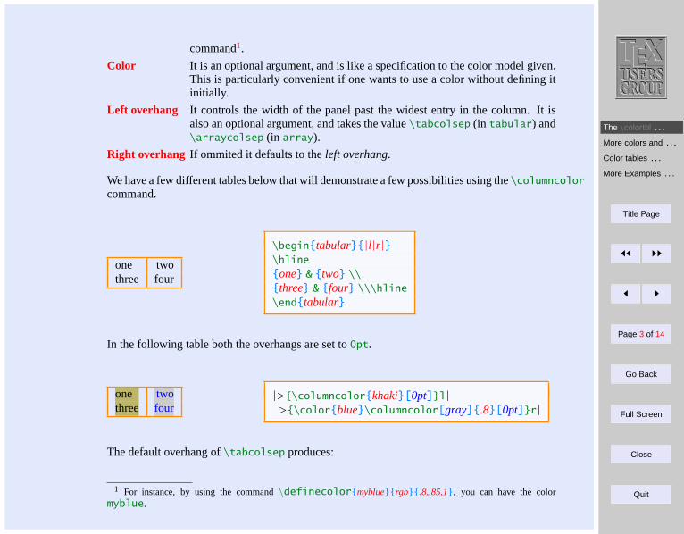
The \colortbl . . .
More colors and . . .
Color tables . . .
More Examples . . .
Title Page
ðð ññ
ð ñ
Page 3 of 14
Go Back
Full Screen
Close
Quit
command1.
Color It is an optional argument, and is like a specification to the color model given.This is particularly convenient if one wants to use a color without defining itinitially.
Left overhang It controls the width of the panel past the widest entry in the column. It isalso an optional argument, and takes the value\tabcolsep (in tabular) and\arraycolsep (in array).
Right overhang If ommited it defaults to theleft overhang.
We have a few different tables below that will demonstrate a few possibilities using the\columncolorcommand.
one twothree four
\begintabular|l|r|\hlineone & two \\three & four \\\hline\endtabular
In the following table both the overhangs are set to0pt.
one twothree four
|>\columncolorkhaki[0pt]l|>\colorblue\columncolor[gray].8[0pt]r|
The default overhang of\tabcolsep produces:
1 For instance, by using the command\definecolormybluergb.8,.85,1, you can have the colormyblue.
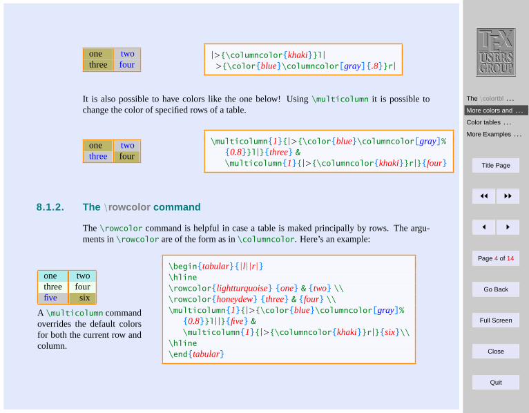
The \colortbl . . .
More colors and . . .
Color tables . . .
More Examples . . .
Title Page
ðð ññ
ð ñ
Page 4 of 14
Go Back
Full Screen
Close
Quit
one twothree four
|>\columncolorkhakil|>\colorblue\columncolor[gray].8r|
It is also possible to have colors like the one below! Using\multicolumn it is possible tochange the color of specified rows of a table.
one twothree four
\multicolumn1|>\colorblue\columncolor[gray]%0.8l|three &\multicolumn1|>\columncolorkhakir|four
8.1.2. The \rowcolor command
The\rowcolor command is helpful in case a table is maked principally by rows. The argu-ments in\rowcolor are of the form as in\columncolor. Here’s an example:
one twothree fourfive six
A \multicolumn commandoverrides the default colorsfor both the current row andcolumn.
\begintabular|l||r|\hline\rowcolorlightturquoise one & two \\\rowcolorhoneydew three & four \\\multicolumn1|>\colorblue\columncolor[gray]%
0.8l||five &\multicolumn1|>\columncolorkhakir|six\\
\hline\endtabular

The \colortbl . . .
More colors and . . .
Color tables . . .
More Examples . . .
Title Page
ðð ññ
ð ñ
Page 5 of 14
Go Back
Full Screen
Close
Quit
8.2. More colors and tricks
In this section we’ll see how to obtain even more colors: colored rules, colored space betweentwo rules, and more.
Colored rules can be easily obtained wherever desired by replacing the| with somethinglike !\colorgreen\vline.
The above trick still leaves the spaces between|| white. In order to obtain colored spaceone can remove the inter glue, and replace it by a colored rule. For instance,
!\colorgreen\vline@\coloryellow\vrule width \doublerulesep!\colorgreen\vline
would change the color of the rules to green, and there would be another yellow rule ofthickness equal to\doublerulesep between the two.
\arrayrulewidth specifies the ‘thickness’ of the rules. The default is set to0.4pt andcan be changed by using, for instance,\setwidth\arrayrulewidth1pt to a value of1pt.
\arrayrulecolor takes the same arguments as\color. It can be specified at any pointin the table. However, if given in the mid table it affects only the rules that are specifiedafter that point, and any vertical rules in the table ‘preamble’ keep their original colors.For example, the command
\setlength\arrayrulewidth1pt\arrayrulecolorblue
would set the\arrayrulewidth to 1pt and the rule color to blue.
\doublerulesep specifies the space between the double rules.
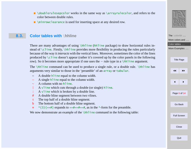
The \colortbl . . .
More colors and . . .
Color tables . . .
More Examples . . .
Title Page
ðð ññ
ð ñ
Page 6 of 14
Go Back
Full Screen
Close
Quit
\doublerulesepcolor works in the same way as\arrayrulecolor, and refers to thecolor between double rules.
\minrowclearance is used for inserting space at any desired row.
8.3. Color tables with \hhline
There are many advantages of using\hhline (hhline package) to draw horizontal rules in-stead of\cline. Firstly, \hhline provides more flexibility in producing the rules particularlybecause of the way itinteractswith the vertical lines. Moreover, sometimes the color of the linesproduced by\cline doesn’t appear (rather it’s covered up by the color panels in the followingrow). So it becomes more appropriate if one uses the− rule type in a\hhline argument.
The\hhline command can be used to produce a single rule, or a double rule.\hhline hasarguments very similar to those in the ‘preamble’ of anarray or tabular.
= A doublehline equal to the column width.− A singlehline equal to the column width.∼ A column with nohline.| A vline which cuts through a double (or single)hline.: A vline which is broken by a double line.# A double hline segment between two vlines.t The top half of a double hline segment.b The bottom half of a double hline segment.∗ *3==# expands to==#==#==#, as in the*-form for the preamble.
We now demonstrate an example of the\hhline command in the following table:
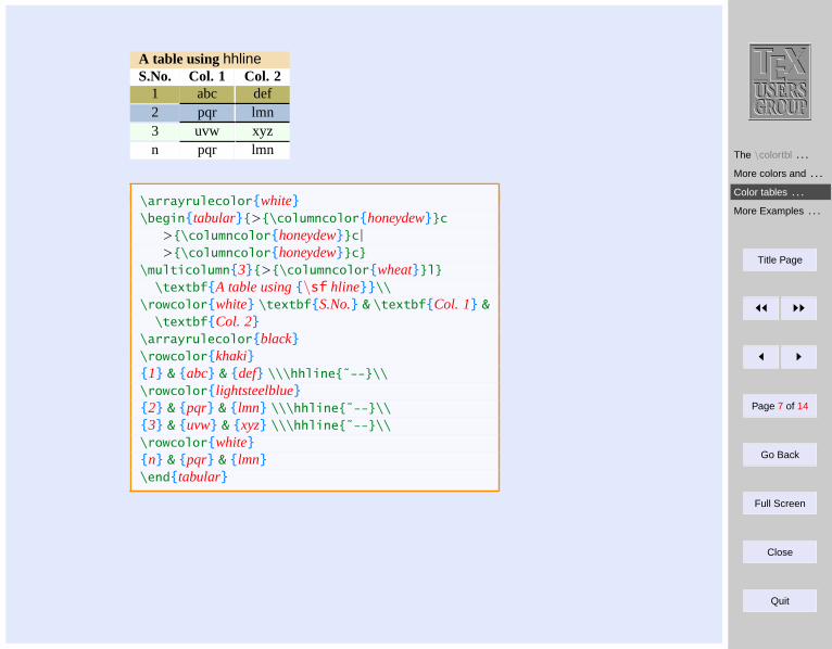
The \colortbl . . .
More colors and . . .
Color tables . . .
More Examples . . .
Title Page
ðð ññ
ð ñ
Page 7 of 14
Go Back
Full Screen
Close
Quit
A table usinghhlineS.No. Col. 1 Col. 2
1 abc def2 pqr lmn3 uvw xyzn pqr lmn
\arrayrulecolorwhite\begintabular>\columncolorhoneydewc
>\columncolorhoneydewc|>\columncolorhoneydewc
\multicolumn3>\columncolorwheatl\textbfA table using\sf hline\\
\rowcolorwhite \textbfS.No. & \textbfCol. 1 &\textbfCol. 2
\arrayrulecolorblack\rowcolorkhaki1 & abc & def \\\hhline˜--\\\rowcolorlightsteelblue2 & pqr & lmn \\\hhline˜--\\3 & uvw & xyz \\\hhline˜--\\\rowcolorwhiten & pqr & lmn\endtabular
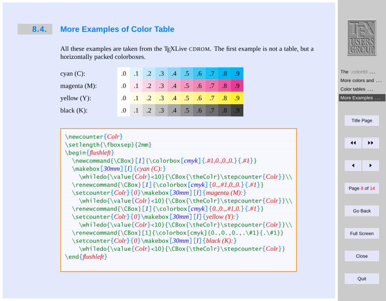
The \colortbl . . .
More colors and . . .
Color tables . . .
More Examples . . .
Title Page
ðð ññ
ð ñ
Page 8 of 14
Go Back
Full Screen
Close
Quit
8.4. More Examples of Color Table
All these examples are taken from the TEXLive CDROM. The first example is not a table, but ahorizontally packed colorboxes.
cyan (C): .0 .1 .2 .3 .4 .5 .6 .7 .8 .9
magenta (M): .0 .1 .2 .3 .4 .5 .6 .7 .8 .9
yellow (Y): .0 .1 .2 .3 .4 .5 .6 .7 .8 .9
black (K): .0 .1 .2 .3 .4 .5 .6 .7 .8 .9
\newcounterColr\setlength\fboxsep2mm\beginflushleft
\newcommand\CBox[1]\colorbox[cmyk].#1,0.,0.,0..#1\makebox[30mm][l]cyan (C):\whiledo\valueColr<10\CBox\theColr\stepcounterColr\\
\renewcommand\CBox[1]\colorbox[cmyk]0.,.#1,0.,0..#1\setcounterColr0\makebox[30mm][l]magenta (M):\whiledo\valueColr<10\CBox\theColr\stepcounterColr\\
\renewcommand\CBox[1]\colorbox[cmyk]0.,0.,.#1,0..#1\setcounterColr0\makebox[30mm][l]yellow (Y):\whiledo\valueColr<10\CBox\theColr\stepcounterColr\\
\renewcommand\CBox[1]\colorbox[cmyk]0.,0.,0.,.\#1.\#1\setcounterColr0\makebox[30mm][l]black (K):\whiledo\valueColr<10\CBox\theColr\stepcounterColr
\endflushleft
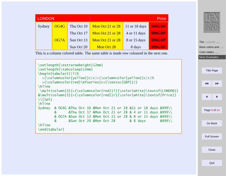
The \colortbl . . .
More colors and . . .
Color tables . . .
More Examples . . .
Title Page
ðð ññ
ð ñ
Page 9 of 14
Go Back
Full Screen
Close
Quit
LONDON Price
Sydney OG4G Thu Oct 10 Mon Oct 21 or 28 11 or 18 days 999GBP
Thu Oct 17 Mon Oct 21 or 28 4 or 11 days 999GBP
OG7A Sun Oct 13 Mon Oct 21 or 28 8 or 15 days 999GBP
Sun Oct 20 Mon Oct 28 8 days 999GBP
This is a column colored table. The same table is made row coloured in the next one.
\setlength\extrarowheight2mm\setlength\tabcolsep2mm\begintabular|l|%
>\columncoloryellowc|c|>\columncoloryellowc|c|%>\columncolorred\bfseriesc<\textscGBP|
\hline\multicolumn3>\columncolorredl\colorwhite\textsfLONDON
&\multicolumn3>\columncolorredr\colorwhite\textsfPrice\\[1pt]\hlineSydney & OG4G &Thu Oct 10 &Mon Oct 21 or 28 &11 or 18 days &999\\
& &Thu Oct 17 &Mon Oct 21 or 28 & 4 or 11 days &999\\& OG7A &Sun Oct 13 &Mon Oct 21 or 28 & 8 or 15 days &999\\& &Sun Oct 20 &Mon Oct 28 & 8 days &999\\
\hline\endtabular
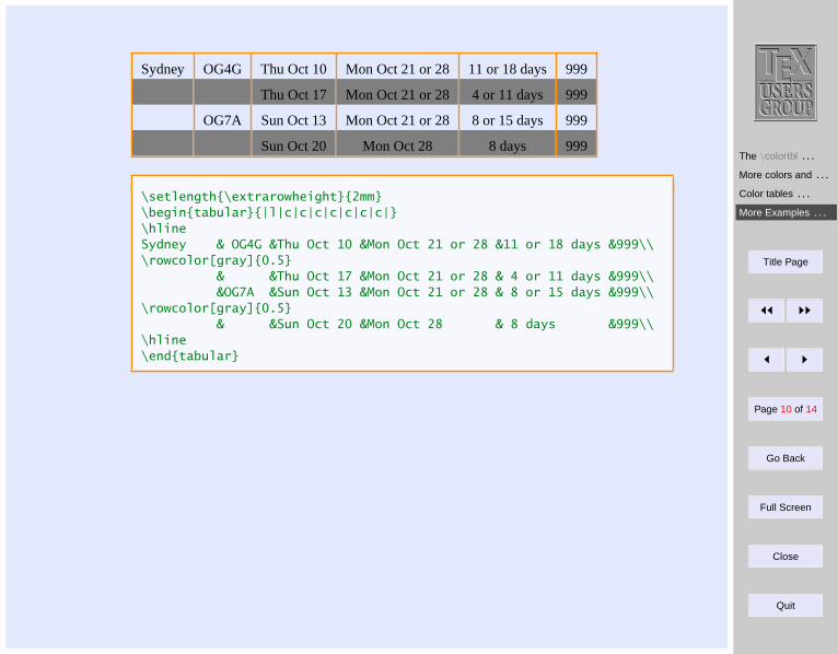
The \colortbl . . .
More colors and . . .
Color tables . . .
More Examples . . .
Title Page
ðð ññ
ð ñ
Page 10 of 14
Go Back
Full Screen
Close
Quit
Sydney OG4G Thu Oct 10 Mon Oct 21 or 28 11 or 18 days 999
Thu Oct 17 Mon Oct 21 or 28 4 or 11 days 999
OG7A Sun Oct 13 Mon Oct 21 or 28 8 or 15 days 999
Sun Oct 20 Mon Oct 28 8 days 999
\setlength\extrarowheight2mm\begintabular|l|c|c|c|c|c|c|c|\hlineSydney & OG4G &Thu Oct 10 &Mon Oct 21 or 28 &11 or 18 days &999\\\rowcolor[gray]0.5
& &Thu Oct 17 &Mon Oct 21 or 28 & 4 or 11 days &999\\&OG7A &Sun Oct 13 &Mon Oct 21 or 28 & 8 or 15 days &999\\
\rowcolor[gray]0.5& &Sun Oct 20 &Mon Oct 28 & 8 days &999\\
\hline\endtabular
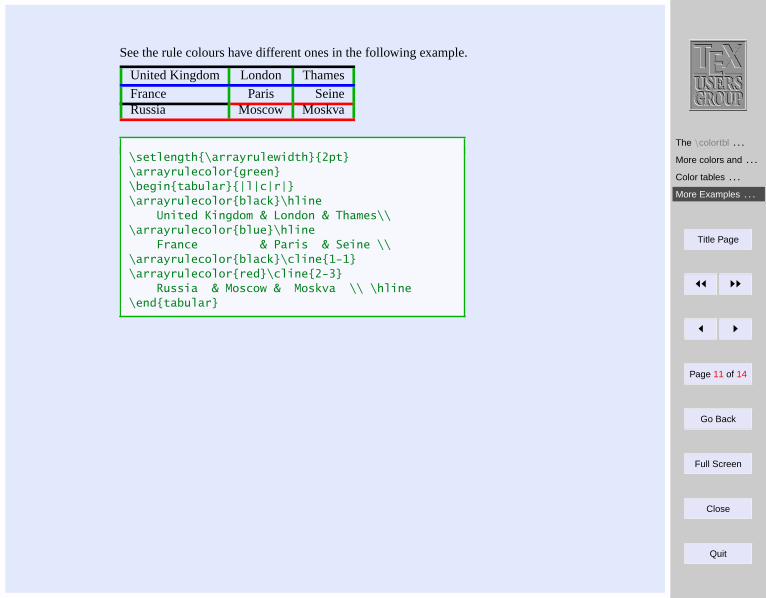
The \colortbl . . .
More colors and . . .
Color tables . . .
More Examples . . .
Title Page
ðð ññ
ð ñ
Page 11 of 14
Go Back
Full Screen
Close
Quit
See the rule colours have different ones in the following example.
United Kingdom London Thames
France Paris SeineRussia Moscow Moskva
\setlength\arrayrulewidth2pt\arrayrulecolorgreen\begintabular|l|c|r|\arrayrulecolorblack\hline
United Kingdom & London & Thames\\\arrayrulecolorblue\hline
France & Paris & Seine \\\arrayrulecolorblack\cline1-1\arrayrulecolorred\cline2-3
Russia & Moscow & Moskva \\ \hline\endtabular
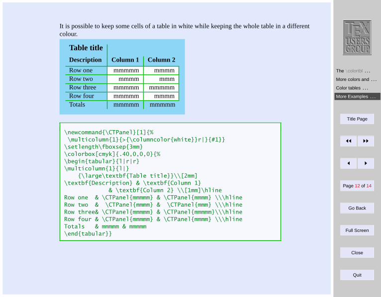
The \colortbl . . .
More colors and . . .
Color tables . . .
More Examples . . .
Title Page
ðð ññ
ð ñ
Page 12 of 14
Go Back
Full Screen
Close
Quit
It is possible to keep some cells of a table in white while keeping the whole table in a differentcolour.
Table title
Description Column 1 Column 2
Row one mmmmm mmmmRow two mmmm mmmRow three mmmmm mmmmmRow four mmmmm mmmmTotals mmmmm mmmmm
\newcommand\CTPanel[1]%\multicolumn1>\columncolorwhiter|#1
\setlength\fboxsep3mm\colorbox[cmyk].40,0,0,0%\begintabularl|r|r\multicolumn1l|
\large\textbfTable title\\[2mm]\textbfDescription & \textbfColumn 1
& \textbfColumn 2 \\[1mm]\hlineRow one & \CTPanelmmmmm & \CTPanelmmmm \\\hlineRow two & \CTPanelmmmm & \CTPanelmmm \\\hlineRow three& \CTPanelmmmmm & \CTPanelmmmmm\\\hlineRow four & \CTPanelmmmmm & \CTPanelmmmm \\\hlineTotals & mmmmm & mmmmm\endtabular
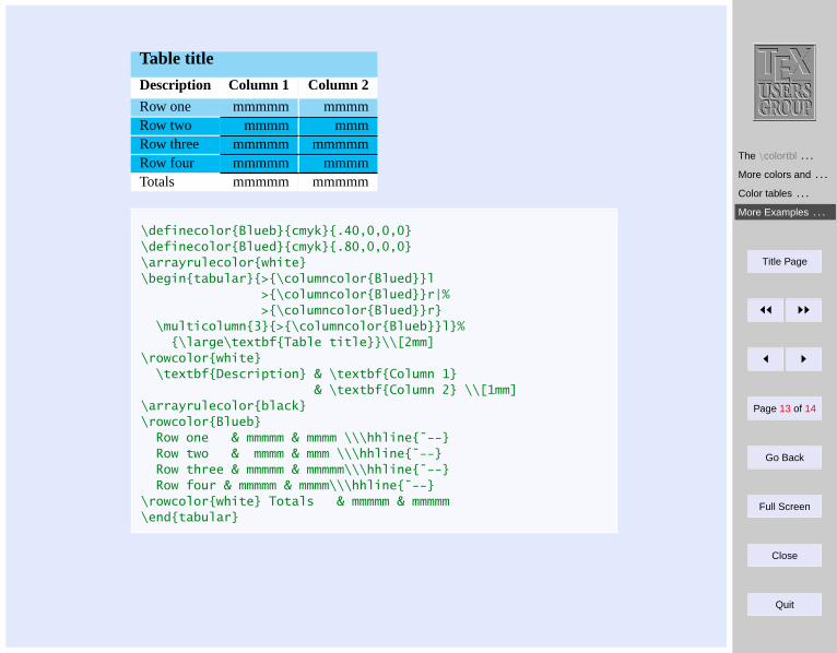
The \colortbl . . .
More colors and . . .
Color tables . . .
More Examples . . .
Title Page
ðð ññ
ð ñ
Page 13 of 14
Go Back
Full Screen
Close
Quit
Table title
Description Column 1 Column 2
Row one mmmmm mmmmRow two mmmm mmmRow three mmmmm mmmmmRow four mmmmm mmmmTotals mmmmm mmmmm
\definecolorBluebcmyk.40,0,0,0\definecolorBluedcmyk.80,0,0,0\arrayrulecolorwhite\begintabular>\columncolorBluedl
>\columncolorBluedr|%>\columncolorBluedr
\multicolumn3>\columncolorBluebl%\large\textbfTable title\\[2mm]
\rowcolorwhite\textbfDescription & \textbfColumn 1
& \textbfColumn 2 \\[1mm]\arrayrulecolorblack\rowcolorBlueb
Row one & mmmmm & mmmm \\\hhline˜--Row two & mmmm & mmm \\\hhline˜--Row three & mmmmm & mmmmm\\\hhline˜--Row four & mmmmm & mmmm\\\hhline˜--
\rowcolorwhite Totals & mmmmm & mmmmm\endtabular
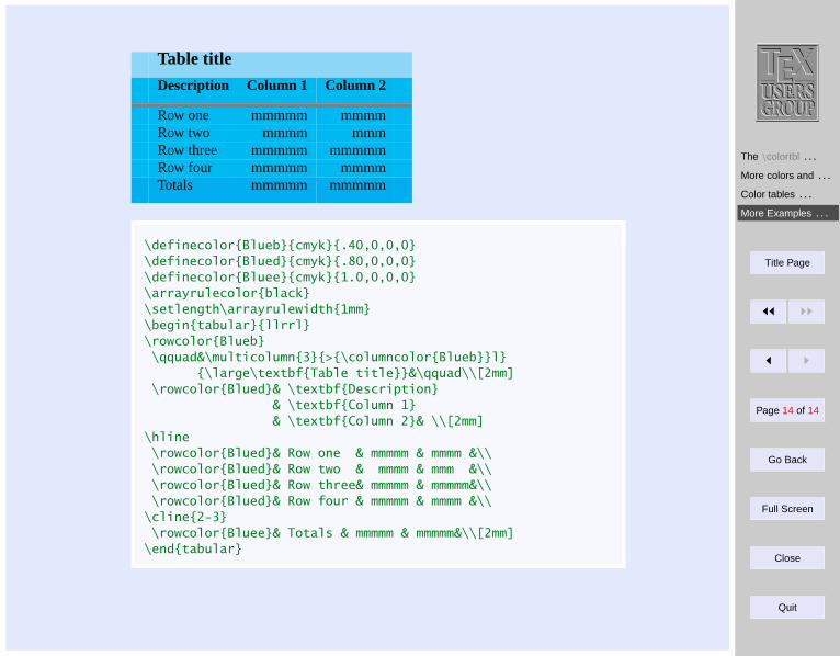
The \colortbl . . .
More colors and . . .
Color tables . . .
More Examples . . .
Title Page
ðð ññ
ð ñ
Page 14 of 14
Go Back
Full Screen
Close
Quit
Table title
Description Column 1 Column 2
Row one mmmmm mmmmRow two mmmm mmmRow three mmmmm mmmmmRow four mmmmm mmmmTotals mmmmm mmmmm
\definecolorBluebcmyk.40,0,0,0\definecolorBluedcmyk.80,0,0,0\definecolorBlueecmyk1.0,0,0,0\arrayrulecolorblack\setlength\arrayrulewidth1mm\begintabularllrrl\rowcolorBlueb\qquad&\multicolumn3>\columncolorBluebl
\large\textbfTable title&\qquad\\[2mm]\rowcolorBlued& \textbfDescription
& \textbfColumn 1& \textbfColumn 2& \\[2mm]
\hline\rowcolorBlued& Row one & mmmmm & mmmm &\\\rowcolorBlued& Row two & mmmm & mmm &\\\rowcolorBlued& Row three& mmmmm & mmmmm&\\\rowcolorBlued& Row four & mmmmm & mmmm &\\\cline2-3\rowcolorBluee& Totals & mmmmm & mmmmm&\\[2mm]\endtabular

Creating Float . . .
Figure Placement
Customizing . . .
Using Graphics . . .
Rotating and . . .
Title Page
JJ II
J I
Page 1 of 13
Go Back
Full Screen
Close
Quit
Indian TEX Users GroupURL: http://www.river-valley.com/tug
9On-line Tutorial on LATEX
The Tutorial TeamIndian TEX Users Group,SJPBuildings, Cotton Hills
Trivandrum695014, INDIA2000
Prof. (Dr.) K. S. S. Nambooripad, Director, Center for Mathematical Sciences, Trivandrum, (Editor); Dr. E. Krishnan,Reader in Mathematics, University College, Trivandrum; Mohit Agarwal, Department of Aerospace Engineering,
Indian Institute of Science, Bangalore; T. Rishi, Focal Image (India) Pvt. Ltd., Trivandrum; L. A. Ajith, Focal Image(India) Pvt. Ltd., Trivandrum; A. M. Shan, Focal Image (India) Pvt. Ltd., Trivandrum; C. V. Radhakrishnan, River
Valley Technologies, Software Technology Park, Trivandrum constitute the Tutorial team
This document is generated from LATEX sources compiled with pdfLATEX v. 14e in anINTEL Pentium III 700 MHz system running Linux kernel version 2.2.14-12. The
packages used are hyperref.sty and pdfscreen.sty
c©2000, Indian TEX Users Group. This document may be distributed under the terms of theLATEX Project Public License, as described in lppl.txt in the base LATEX distribution, either
version 1.0 or, at your option, any later version
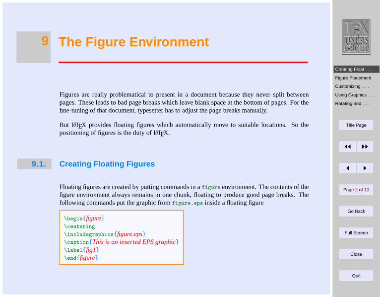
Creating Float . . .
Figure Placement
Customizing . . .
Using Graphics . . .
Rotating and . . .
Title Page
JJ II
J I
Page 2 of 13
Go Back
Full Screen
Close
Quit
9 The Figure Environment
Figures are really problematical to present in a document because they never split betweenpages. These leads to bad page breaks which leave blank space at the bottom of pages. For thefine-tuning of that document, typesetter has to adjust the page breaks manually.
But LATEX provides floating figures which automatically move to suitable locations. So thepositioning of figures is the duty of LATEX.
9.1. Creating Floating Figures
Floating figures are created by putting commands in afigure environment. The contents of thefigure environment always remains in one chunk, floating to produce good page breaks. Thefollowing commands put the graphic fromfigure.eps inside a floating figure
\beginfigure\centering
\includegraphicsfigure.eps\captionThis is an inserted EPS graphic\labelfig1\endfigure
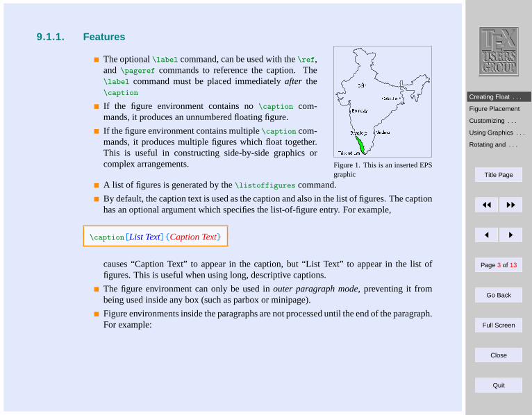
Creating Float . . .
Figure Placement
Customizing . . .
Using Graphics . . .
Rotating and . . .
Title Page
JJ II
J I
Page 3 of 13
Go Back
Full Screen
Close
Quit
9.1.1. Features
The optional\label command, can be used with the\ref,and \pageref commands to reference the caption. The\label command must be placed immediatelyafter the\caption
If the figure environment contains no\caption com-mands, it produces an unnumbered floating figure.
If the figure environment contains multiple\caption com-mands, it produces multiple figures which float together.This is useful in constructing side-by-side graphics orcomplex arrangements.
Figure 1. This is an inserted EPSgraphic
A list of figures is generated by the\listoffigures command.
By default, the caption text is used as the caption and also in the list of figures. The captionhas an optional argument which specifies the list-of-figure entry. For example,
\caption[List Text]Caption Text
causes “Caption Text” to appear in the caption, but “List Text” to appear in the list offigures. This is useful when using long, descriptive captions.
The figure environment can only be used inouter paragraph mode, preventing it frombeing used inside any box (such as parbox or minipage).
Figure environments inside the paragraphs are not processed until the end of the paragraph.For example:
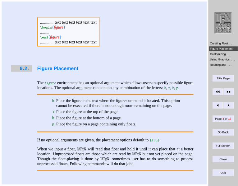
Creating Float . . .
Figure Placement
Customizing . . .
Using Graphics . . .
Rotating and . . .
Title Page
JJ II
J I
Page 4 of 13
Go Back
Full Screen
Close
Quit
............. text text text text text text\beginfigure.........\endfigure............. text text text text text text
9.2. Figure Placement
Thefigure environment has an optional argument which allows users to specify possible figurelocations. The optional argument can contain any combination of the letters:h, t, b, p.
h Place the figure in the text where the figure command is located. This optioncannot be executed if there is not enough room remaining on the page.
t Place the figure at the top of the page.
b Place the figure at the bottom of a page.
p Place the figure on a page containing only floats.
If no optional arguments are given, the placement options default to[tbp].
When we input a float, LATEX will read that float and hold it until it can place that at a betterlocation. Unprocessed floats are those which are read by LATEX but not yet placed on the page.Though the float-placing is done by LATEX, sometimes user has to do something to processunprocessed floats. Following commands will do that job:
Creating Float . . .
Figure Placement
Customizing . . .
Using Graphics . . .
Rotating and . . .
Title Page
JJ II
J I
Page 5 of 13
Go Back
Full Screen
Close
Quit
\clearpage This command places unprocessed floats and starts a new page.
\FloatBarrier This command causes all unprocessed floats to be processed. Thisis provided by theplaceins package. It does not start a new page,unlike\clearpage.
Since it is often desirable to keep floats in the section in which they were issued, thesection
option
\usepackage[section]placeins
redefines the\section command, inserting a\FloatBarrier command before each section.Note that this option is very strict. This option does not allow a float from the old section toappear at the bottom of the page, since that is after the start of a new section.
Thebelow option
\usepackage[below]placeins
is a less-restrictive version of thesection option. It allows floats to be placed after the beginningof a new section, provided that some of the old section appears on the page.
\afterpage/\clearpage Theafterpage package provides the\afterpage command whichexecutes a command at the next naturally-ocurring page break.
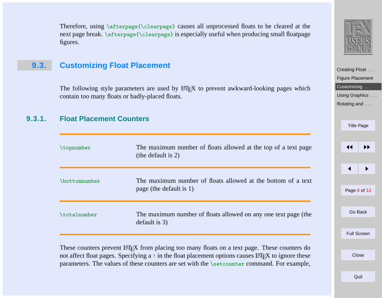
Creating Float . . .
Figure Placement
Customizing . . .
Using Graphics . . .
Rotating and . . .
Title Page
JJ II
J I
Page 6 of 13
Go Back
Full Screen
Close
Quit
Therefore, using\afterpage\clearpage causes all unprocessed floats to be cleared at thenext page break.\afterpage\clearpage is especially useful when producing small floatpagefigures.
9.3. Customizing Float Placement
The following style parameters are used by LATEX to prevent awkward-looking pages whichcontain too many floats or badly-placed floats.
9.3.1. Float Placement Counters
\topnumber The maximum number of floats allowed at the top of a text page(the default is 2)
\bottomnumber The maximum number of floats allowed at the bottom of a textpage (the default is 1)
\totalnumber The maximum number of floats allowed on any one text page (thedefault is 3)
These counters prevent LATEX from placing too many floats on a text page. These counters donot affect float pages. Specifying a! in the float placement options causes LATEX to ignore theseparameters. The values of these counters are set with the\setcounter command. For example,
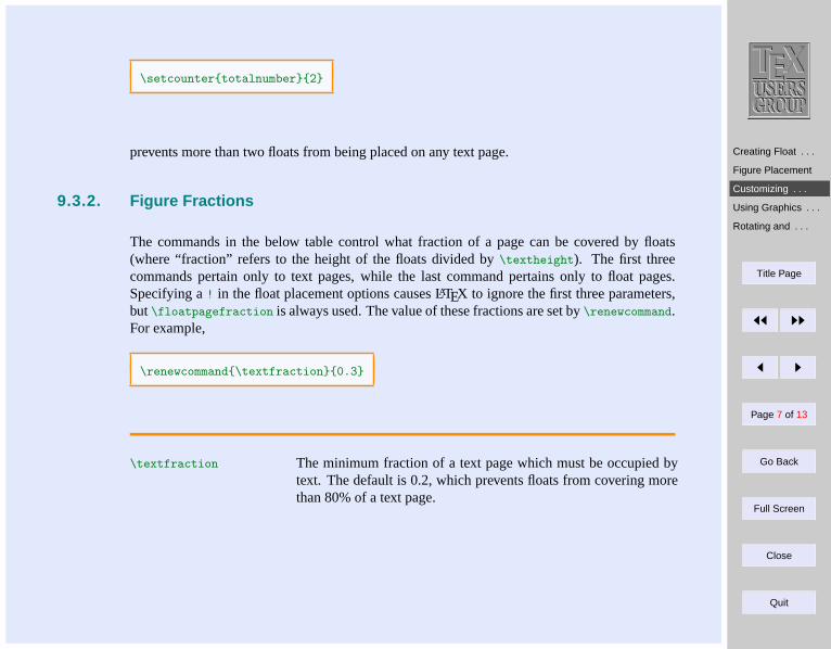
Creating Float . . .
Figure Placement
Customizing . . .
Using Graphics . . .
Rotating and . . .
Title Page
JJ II
J I
Page 7 of 13
Go Back
Full Screen
Close
Quit
\setcountertotalnumber2
prevents more than two floats from being placed on any text page.
9.3.2. Figure Fractions
The commands in the below table control what fraction of a page can be covered by floats(where “fraction” refers to the height of the floats divided by\textheight). The first threecommands pertain only to text pages, while the last command pertains only to float pages.Specifying a! in the float placement options causes LATEX to ignore the first three parameters,but\floatpagefraction is always used. The value of these fractions are set by\renewcommand.For example,
\renewcommand\textfraction0.3
\textfraction The minimum fraction of a text page which must be occupied bytext. The default is 0.2, which prevents floats from covering morethan 80% of a text page.
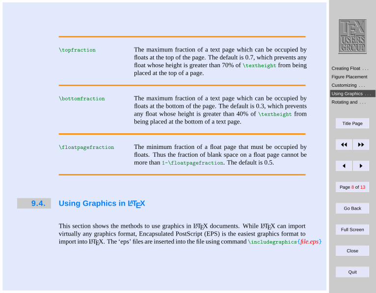
Creating Float . . .
Figure Placement
Customizing . . .
Using Graphics . . .
Rotating and . . .
Title Page
JJ II
J I
Page 8 of 13
Go Back
Full Screen
Close
Quit
\topfraction The maximum fraction of a text page which can be occupied byfloats at the top of the page. The default is 0.7, which prevents anyfloat whose height is greater than 70% of\textheight from beingplaced at the top of a page.
\bottomfraction The maximum fraction of a text page which can be occupied byfloats at the bottom of the page. The default is 0.3, which preventsany float whose height is greater than 40% of\textheight frombeing placed at the bottom of a text page.
\floatpagefraction The minimum fraction of a float page that must be occupied byfloats. Thus the fraction of blank space on a float page cannot bemore than1-\floatpagefraction. The default is 0.5.
9.4. Using Graphics in L ATEX
This section shows the methods to use graphics in LATEX documents. While LATEX can importvirtually any graphics format, Encapsulated PostScript (EPS) is the easiest graphics format toimport into LATEX. The ‘eps’ files are inserted into the file using command\includegraphicsfile.eps
Creating Float . . .
Figure Placement
Customizing . . .
Using Graphics . . .
Rotating and . . .
Title Page
JJ II
J I
Page 9 of 13
Go Back
Full Screen
Close
Quit
9.4.1. The \includegraphics Command
\includegraphics[options]filename
Following are the options available in\includegraphics command:
width The width of the graphics (in any of the accepted TEX units).
height The height of the graphics (in any of the accepted TEX units).
totalheight The totalheight of the graphics (in any of the accepted TEX units).
scale Scale factor for the graphic. Specifyingscale=2makes the graphic twiceas large as its natural size.
angle Specifies the angle of rotation, in degrees, with a counter-clockwise(anti-clockwise) rotation being positive.
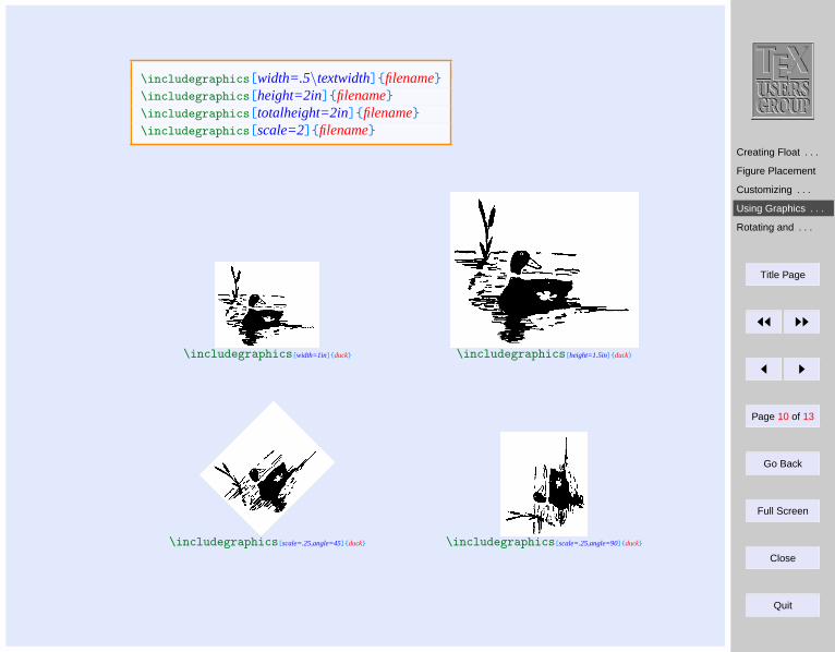
Creating Float . . .
Figure Placement
Customizing . . .
Using Graphics . . .
Rotating and . . .
Title Page
JJ II
J I
Page 10 of 13
Go Back
Full Screen
Close
Quit
\includegraphics[width=.5\textwidth]filename\includegraphics[height=2in]filename\includegraphics[totalheight=2in]filename\includegraphics[scale=2]filename
\includegraphics[width=1in]duck \includegraphics[height=1.5in]duck
\includegraphics[scale=.25,angle=45]duck \includegraphics[scale=.25,angle=90]duck
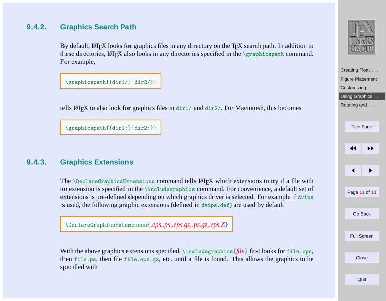
Creating Float . . .
Figure Placement
Customizing . . .
Using Graphics . . .
Rotating and . . .
Title Page
JJ II
J I
Page 11 of 13
Go Back
Full Screen
Close
Quit
9.4.2. Graphics Search Path
By default, LATEX looks for graphics files in any directory on the TEX search path. In addition tothese directories, LATEX also looks in any directories specified in the\graphicspath command.For example,
\graphicspathdir1/dir2/
tells LATEX to also look for graphics files indir1/ anddir2/. For Macintosh, this becomes
\graphicspathdir1:dir2:
9.4.3. Graphics Extensions
The\DeclareGraphicsExtensions command tells LATEX which extensions to try if a file withno extension is specified in the\includegraphics command. For convenience, a default set ofextensions is pre-defined depending on which graphics driver is selected. For example ifdvips
is used, the following graphic extensions (defined indvips.def) are used by default
\DeclareGraphicsExtensions.eps,.ps,.eps.gz,.ps.gz,.eps.Z
With the above graphics extensions specified,\includegraphicsfile first looks forfile.eps,thenfile.ps, then filefile.eps.gz, etc. until a file is found. This allows the graphics to bespecified with
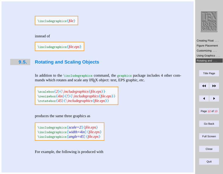
Creating Float . . .
Figure Placement
Customizing . . .
Using Graphics . . .
Rotating and . . .
Title Page
JJ II
J I
Page 12 of 13
Go Back
Full Screen
Close
Quit
\includegraphicsfile
instead of
\includegraphicsfile.eps
9.5. Rotating and Scaling Objects
In addition to the\includegraphics command, thegraphicx package includes 4 other com-mands which rotates and scale any LATEX object: text, EPS graphic, etc.
\scalebox2\includegraphicsfile.eps\resizebox4in!\includegraphicsfile.eps\rotatebox45\includegraphicsfile.eps
produces the same three graphics as
\includegraphics[scale=2]file.eps\includegraphics[width=4in]file.eps\includegraphics[angle=45]file.eps
For example, the following is produced with
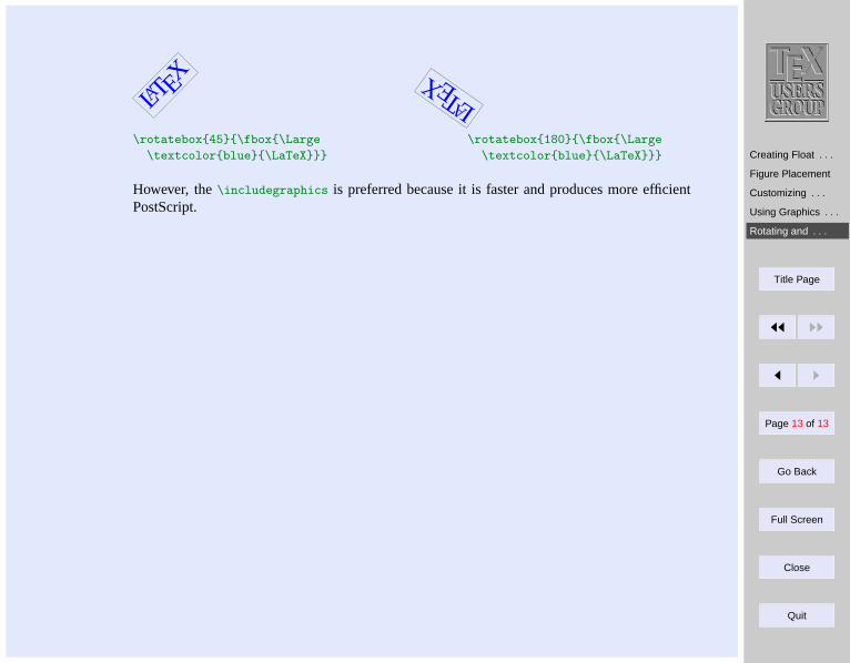
Creating Float . . .
Figure Placement
Customizing . . .
Using Graphics . . .
Rotating and . . .
Title Page
JJ II
J I
Page 13 of 13
Go Back
Full Screen
Close
Quit
LATEX
LATEX
\rotatebox45\fbox\Large
\textcolorblue\LaTeX
\rotatebox180\fbox\Large
\textcolorblue\LaTeX
However, the\includegraphics is preferred because it is faster and produces more efficientPostScript.
Introduction
natbib
Title Page
JJ II
J I
Page 1 of 11
Go Back
Full Screen
Close
Quit
Indian TEX Users GroupURL: http://www.river-valley.com/tug
10On-line Tutorial on LATEX
The Tutorial TeamIndian TEX Users Group,SJPBuildings, Cotton Hills
Trivandrum 695014,INDIA
2000
Prof. (Dr.) K. S. S. Nambooripad, Director, Center for Mathematical Sciences, Trivandrum, (Editor); Dr. E. Krishnan,Reader in Mathematics, University College, Trivandrum; Mohit Agarwal, Department of Aerospace Engineering,
Indian Institute of Science, Bangalore; T. Rishi, Focal Image (India) Pvt. Ltd., Trivandrum; L. A. Ajith, Focal Image(India) Pvt. Ltd., Trivandrum; A. M. Shan, Focal Image (India) Pvt. Ltd., Trivandrum; C. V. Radhakrishnan, River
Valley Technologies, Software Technology Park, Trivandrum constitute the Tutorial team
This document is generated from LATEX sources compiled with pdfLATEX v. 14e in anINTEL Pentium III 700 MHz system running Linux kernel version 2.2.14-12. The
packages used are hyperref.sty and pdfscreen.sty
c©2000, Indian TEX Users Group. This document may be distributed under the terms of theLATEX Project Public License, as described in lppl.txt in the base LATEX distribution, either
version 1.0 or, at your option, any later version
Introduction
natbib
Title Page
JJ II
J I
Page 2 of 11
Go Back
Full Screen
Close
Quit
10 Bibliography
10.1. Introduction
Bibliography is the environment, which helps the author to cross-reference one publication fromthe list of sources at the end of the document. Bibliography needs consistency, LATEX helpsauthor to write well structured bibliography, because this is how LATEX works—by specifyingstructure.
It is easy to convert the style of bibliography to publisher’s require, without touching the codeinside the bibliography. We can maintain a bibliographic data base using the program BIBTEX.While preparing the articles, we can extract the needed references in needed style from this database. Harvard and natbib are widely used packages for generating bibliography.
To produce bibliography, we have the environmentthebibliography1, which acts similar toenu-merate environment. Here we use\bibitem and \cite commands, which do the operationsimilar to \label and\ref. That means in the place of citation, it will produce number orauthor-year code connected with list of references at the end.
1 Bibiliography environment need two compilation. In first compilation it will generate file with aux extension, wherecitation andbibcite will be marked and in second compilation\citewill be replaced by numeral or author-year code.
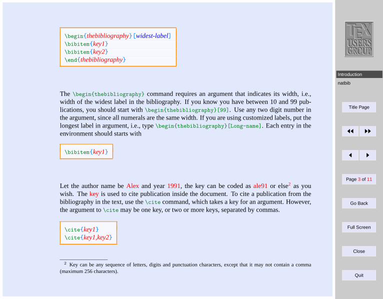
Introduction
natbib
Title Page
JJ II
J I
Page 3 of 11
Go Back
Full Screen
Close
Quit
\beginthebibliography[widest-label]\bibitemkey1\bibitemkey2\endthebibliography
The \beginthebibliography command requires an argument that indicates its width, i.e.,width of the widest label in the bibliography. If you know you have between 10 and 99 pub-lications, you should start with\beginthebibliography[99]. Use any two digit number inthe argument, since all numerals are the same width. If you are using customized labels, put thelongest label in argument, i.e., type\beginthebibliography[Long-name]. Each entry in theenvironment should starts with
\bibitemkey1
Let the author name beAlex and year1991, the key can be coded asale91or else2 as youwish. Thekey is used to cite publication inside the document. To cite a publication from thebibliography in the text, use the\cite command, which takes a key for an argument. However,the argument to\cite may be one key, or two or more keys, separated by commas.
\citekey1\citekey1,key2
2 Key can be any sequence of letters, digits and punctuation characters, except that it may not contain a comma(maximum 256 characters).
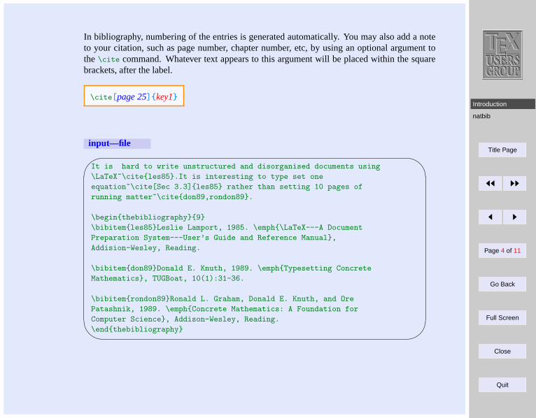
Introduction
natbib
Title Page
JJ II
J I
Page 4 of 11
Go Back
Full Screen
Close
Quit
In bibliography, numbering of the entries is generated automatically. You may also add a noteto your citation, such as page number, chapter number, etc, by using an optional argument tothe\cite command. Whatever text appears to this argument will be placed within the squarebrackets, after the label.
\cite[page 25]key1
input—file'
&
$
%
It is hard to write unstructured and disorganised documents using
\LaTeX~\citeles85.It is interesting to type set one
equation~\cite[Sec 3.3]les85 rather than setting 10 pages of
running matter~\citedon89,rondon89.
\beginthebibliography9
\bibitemles85Leslie Lamport, 1985. \emph\LaTeX---A Document
Preparation System---User’s Guide and Reference Manual,
Addision-Wesley, Reading.
\bibitemdon89Donald E. Knuth, 1989. \emphTypesetting Concrete
Mathematics, TUGBoat, 10(1):31-36.
\bibitemrondon89Ronald L. Graham, Donald E. Knuth, and Ore
Patashnik, 1989. \emphConcrete Mathematics: A Foundation for
Computer Science, Addison-Wesley, Reading.
\endthebibliography

Introduction
natbib
Title Page
JJ II
J I
Page 5 of 11
Go Back
Full Screen
Close
Quit
output—dvi
It is hard to write unstructured and disorganised documents using LATEX[1]. It is interesting to typeset one equation[1, Sec 3.3] rather than setting 10 pages of running matter[2,3].
Bibliography
[1] Leslie Lamport, 1985.LATEX—A Document Preparation System—User’s Guide and Refer-ence Manual, Addision-Wesley, Reading.
[2] Donald E. Knuth, 1989.Typesetting Concrete Mathematics, TUGBoat, 10(1):31-36.[3] Ronald L. Graham, Donald E. Knuth, and Ore Patashnik, 1989.Concrete Mathematics: A
Foundation for Computer Science, Addison-Wesley, Reading.
10.2. natbib
Thenatbib package is widely used for generating bibliography, because of it’s flexible interfacefor most of the available bibliographic styles. Thenatbib.sty package is a re-implementationof the LATEX \cite command, to work with both author–year and numerical citations. It iscompatible with the standard bibliographic style files, such asplain.bst, as well as with thosefor harvard, apalike, chicago, astron, authordate, and of coursenatbib.sty. To load the package:
\usepackage[options]natbib
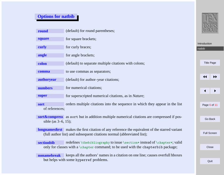
Introduction
natbib
Title Page
JJ II
J I
Page 6 of 11
Go Back
Full Screen
Close
Quit
Options for natbib
round (default) for round parentheses;
square for square brackets;
curly for curly braces;
angle for angle brackets;
colon (default) to separate multiple citations with colons;
comma to use commas as separators;
authoryear (default) for author–year citations;
numbers for numerical citations;
super for superscripted numerical citations, as inNature;
sort orders multiple citations into the sequence in which they appear in the listof references;
sort&compress assort but in addition multiple numerical citations are compressed if pos-sible (as 3–6, 15);
longnamesfirst makes the first citation of any reference the equivalent of the starred variant(full author list) and subsequent citations normal (abbreviated list);
sectionbib redefines\thebibliography to issue\section* instead of\chapter*; validonly for classes with a\chapter command; to be used with thechapterbib package;
nonamebreak keeps all the authors’ names in a citation on one line; causes overfull hboxesbut helps with somehyperref problems.
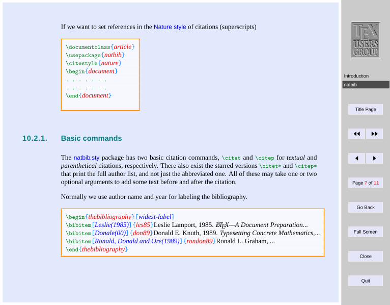
Introduction
natbib
Title Page
JJ II
J I
Page 7 of 11
Go Back
Full Screen
Close
Quit
If we want to set references in theNature style of citations (superscripts)
\documentclassarticle\usepackagenatbib\citestylenature\begindocument. . . . . . .
. . . . . . .
\enddocument
10.2.1. Basic commands
The natbib.sty package has two basic citation commands,\citet and\citep for textualandparentheticalcitations, respectively. There also exist the starred versions\citet* and\citep*that print the full author list, and not just the abbreviated one. All of these may take one or twooptional arguments to add some text before and after the citation.
Normally we use author name and year for labeling the bibliography.
\beginthebibliography[widest-label]\bibitem[Leslie(1985)]les85Leslie Lamport, 1985.LATEX—A Document Preparation...\bibitem[Donale(00)]don89Donald E. Knuth, 1989.Typesetting Concrete Mathematics,...\bibitem[Ronald, Donald and Ore(1989)]rondon89Ronald L. Graham, ...\endthebibliography
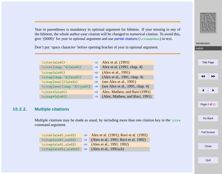
Introduction
natbib
Title Page
JJ II
J I
Page 8 of 11
Go Back
Full Screen
Close
Quit
Year in parentheses is mandatory in optional argument for bibitem. If year missing in any ofthe bibitem, the whole author-year citation will be changed to numerical citation. To avoid this,give ‘(0000)’ for year in optional argument and usepartial citations (\citeauthor) in text.
Don’t put ‘space character’ before opening bracket of year in optional argument.
\citetale91 ⇒ Alex et al. (1991)\citet[chap.~4]ale91 ⇒ Alex et al. (1991, chap. 4)
\citepale91 ⇒ (Alex et al., 1991)\citep[chap.~4]ale91 ⇒ (Alex et al., 1991, chap. 4)\citep[see][]ale91 ⇒ (see Alex et al., 1991)\citep[see][chap.~4]jon91 ⇒ (see Alex et al., 1991, chap. 4)
\citet*ale91 ⇒ Alex, Mathew, and Ravi (1991)\citep*ale91 ⇒ (Alex, Mathew, and Ravi, 1991)
10.2.2. Multiple citations
Multiple citations may be made as usual, by including more than one citation key in the\cite
command argument.
\citetale91,rav92 ⇒ Alex et al. (1991); Ravi et al. (1992)\citepale91,rav92 ⇒ (Alex et al., 1991; Ravi et al. 1992)\citepale91,ale92 ⇒ (Alex et al., 1991, 1992)\citepale91a,ale91b ⇒ (Alex et al., 1991a,b)
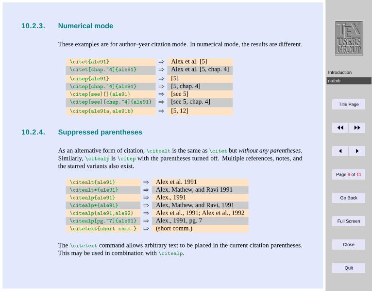
Introduction
natbib
Title Page
JJ II
J I
Page 9 of 11
Go Back
Full Screen
Close
Quit
10.2.3. Numerical mode
These examples are for author–year citation mode. In numerical mode, the results are different.
\citetale91 ⇒ Alex et al. [5]\citet[chap.~4]ale91 ⇒ Alex et al. [5, chap. 4]
\citepale91 ⇒ [5]\citep[chap.~4]ale91 ⇒ [5, chap. 4]\citep[see][]ale91 ⇒ [see 5]\citep[see][chap.~4]ale91 ⇒ [see 5, chap. 4]
\citepale91a,ale91b ⇒ [5, 12]
10.2.4. Suppressed parentheses
As an alternative form of citation,\citealt is the same as\citet butwithout any parentheses.Similarly, \citealp is \citep with the parentheses turned off. Multiple references, notes, andthe starred variants also exist.
\citealtale91 ⇒ Alex et al. 1991\citealt*ale91 ⇒ Alex, Mathew, and Ravi 1991\citealpale91 ⇒ Alex., 1991\citealp*ale91 ⇒ Alex, Mathew, and Ravi, 1991\citealpale91,ale92 ⇒ Alex et al., 1991; Alex et al., 1992\citealp[pg.~7]ale91 ⇒ Alex., 1991, pg. 7\citetextshort comm. ⇒ (short comm.)
The\citetext command allows arbitrary text to be placed in the current citation parentheses.This may be used in combination with\citealp.
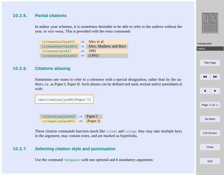
Introduction
natbib
Title Page
JJ II
J I
Page 10 of 11
Go Back
Full Screen
Close
Quit
10.2.5. Partial citations
In author–year schemes, it is sometimes desirable to be able to refer to the authors without theyear, or vice versa. This is provided with the extra commands
\citeauthorale91 ⇒ Alex et al.\citeauthor*ale91 ⇒ Alex, Mathew, and Ravi\citeyearale91 ⇒ 1991\citeyearparale91 ⇒ (1991)
10.2.6. Citations aliasing
Sometimes one wants to refer to a reference with a special designation, rather than by the au-thors, i.e. as Paper I, Paper II. Such aliases can be defined and used, textual and/or parentheticalwith:
\defcitealiasjon90Paper~I
\citetaliasale91 ⇒ Paper I\citepaliasale91 ⇒ (Paper I)
These citation commands function much like\citet and\citep: they may take multiple keysin the argument, may contain notes, and are marked as hyperlinks.
10.2.7. Selecting citation style and punctuation
Use the command\bibpunct with one optional and 6 mandatory arguments:
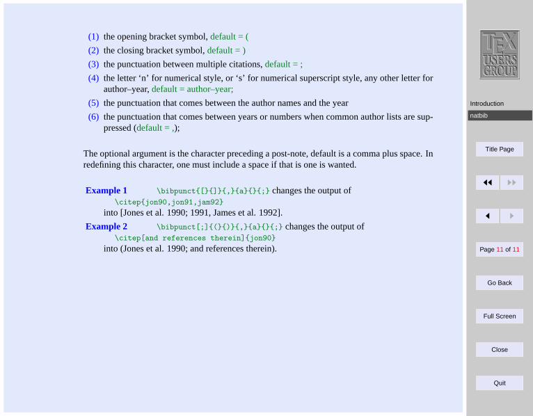
Introduction
natbib
Title Page
JJ II
J I
Page 11 of 11
Go Back
Full Screen
Close
Quit
(1) the opening bracket symbol,default = (
(2) the closing bracket symbol,default = )
(3) the punctuation between multiple citations,default = ;
(4) the letter ‘n’ for numerical style, or ‘s’ for numerical superscript style, any other letter forauthor–year,default = author–year;
(5) the punctuation that comes between the author names and the year
(6) the punctuation that comes between years or numbers when common author lists are sup-pressed (default = ,);
The optional argument is the character preceding a post-note, default is a comma plus space. Inredefining this character, one must include a space if that is one is wanted.
Example 1 \bibpunct[],a; changes the output of\citepjon90,jon91,jam92
into [Jones et al. 1990; 1991, James et al. 1992].
Example 2 \bibpunct[;](),a; changes the output of\citep[and references therein]jon90
into (Jones et al. 1990; and references therein).
Introduction
Maths in text
Fraction
Equation
Definitions for . . .
AMS-LaTeX
Mathematical . . .
Accents and For . . .
Title Page
JJ II
J I
Page 1 of 31
Go Back
Full Screen
Close
Quit
Indian TEX Users Group: http://www.river-valley.com/tug
11On-line Tutorial on LATEX
The Tutorial TeamIndian TEX Users Group, Buildings, Cotton Hills
Trivandrum 695014, 2000
Prof. (Dr.) K. S. S. Nambooripad, Director, Center for Mathematical Sciences, Trivandrum, (Editor); Dr. E. Krishnan, Readerin Mathematics, University College, Trivandrum; Mohit Agarwal, Department of Aerospace Engineering, Indian Institute of
Science, Bangalore; T. Rishi, Focal Image (India) Pvt. Ltd., Trivandrum; L. A. Ajith, Focal Image (India) Pvt. Ltd.,Trivandrum; A. M. Shan, Focal Image (India) Pvt. Ltd., Trivandrum; C. V. Radhakrishnan, River Valley Technologies,
Software Technology Park, Trivandrum constitute the Tutorial team
This document is generated from LATEX sources compiled with pdfLATEX v. 14e in an INTEL
Pentium III 700 MHz system running Linux kernel version 2.2.14-12. The packages usedare hyperref.sty and pdfscreen.sty
c©2000, Indian TEX Users Group. This document may be distributed under the terms of the LATEXProject Public License, as described in lppl.txt in the base LATEX distribution, either version 1.0
or, at your option, any later version
Introduction
Maths in text
Fraction
Equation
Definitions for . . .
AMS-LaTeX
Mathematical . . .
Accents and For . . .
Title Page
JJ II
J I
Page 2 of 31
Go Back
Full Screen
Close
Quit
11 Mathematics
11.1. Introduction
TEX is at its best while producing mathematical documents. If you want to test the power ofTEX, do typeset some mathematics. In the foreword of the TEX book, Knuth writes: “TEX is anew typesetting system intended for the creation of beautiful books—and especially for booksthat contain a lot of mathematics”.
LATEX has a special mode for typesetting mathematics. Mathematical text within a paragraph (in-line) is entered between \( and \), between $ and $ or between \beginmath and \endmath.
Normally larger mathematical equations and formula are typesetted in separate lines, in displaymode. To produce this, we enclose them between \[ and \], between $$ and $$ or between\begindisplaymath and \enddisplaymath. This produces formula, which are not num-bered. If we want to produce equation number, we have to use equation environment.
The spacing for both in-line and displayed mathematics is completely controlled by TEX.
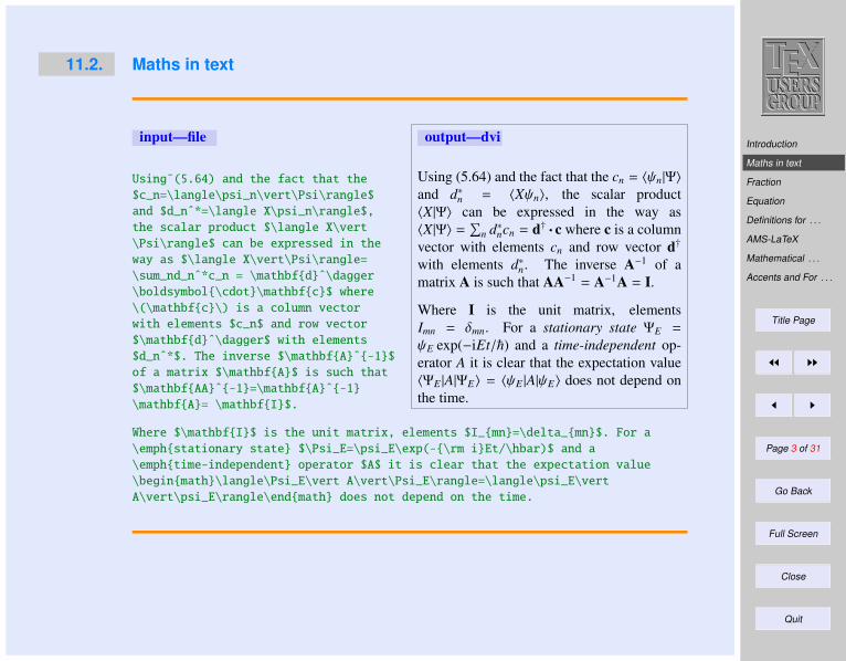
Introduction
Maths in text
Fraction
Equation
Definitions for . . .
AMS-LaTeX
Mathematical . . .
Accents and For . . .
Title Page
JJ II
J I
Page 3 of 31
Go Back
Full Screen
Close
Quit
11.2. Maths in text
input—file
Using˜(5.64) and the fact that the
$c_n=\langle\psi_n\vert\Psi\rangle$
and $d_nˆ*=\langle X\psi_n\rangle$,
the scalar product $\langle X\vert
\Psi\rangle$ can be expressed in the
way as $\langle X\vert\Psi\rangle=
\sum_nd_nˆ*c_n = \mathbfdˆ\dagger
\boldsymbol\cdot\mathbfc$ where
\(\mathbfc\) is a column vector
with elements $c_n$ and row vector
$\mathbfdˆ\dagger$ with elements
$d_nˆ*$. The inverse $\mathbfAˆ-1$
of a matrix $\mathbfA$ is such that
$\mathbfAAˆ-1=\mathbfAˆ-1
\mathbfA= \mathbfI$.
output—dvi
Using (5.64) and the fact that the cn = 〈ψn|Ψ〉
and d∗n = 〈Xψn〉, the scalar product〈X|Ψ〉 can be expressed in the way as〈X|Ψ〉 =
∑n d∗ncn = d† · c where c is a column
vector with elements cn and row vector d†with elements d∗n. The inverse A−1 of amatrix A is such that AA−1 = A−1A = I.
Where I is the unit matrix, elementsImn = δmn. For a stationary state ΨE =
ψE exp(−iEt/~) and a time-independent op-erator A it is clear that the expectation value〈ΨE |A|ΨE〉 = 〈ψE |A|ψE〉 does not depend onthe time.
Where $\mathbfI$ is the unit matrix, elements $I_mn=\delta_mn$. For a
\emphstationary state $\Psi_E=\psi_E\exp(-\rm iEt/\hbar)$ and a
\emphtime-independent operator $A$ it is clear that the expectation value
\beginmath\langle\Psi_E\vert A\vert\Psi_E\rangle=\langle\psi_E\vert
A\vert\psi_E\rangle\endmath does not depend on the time.
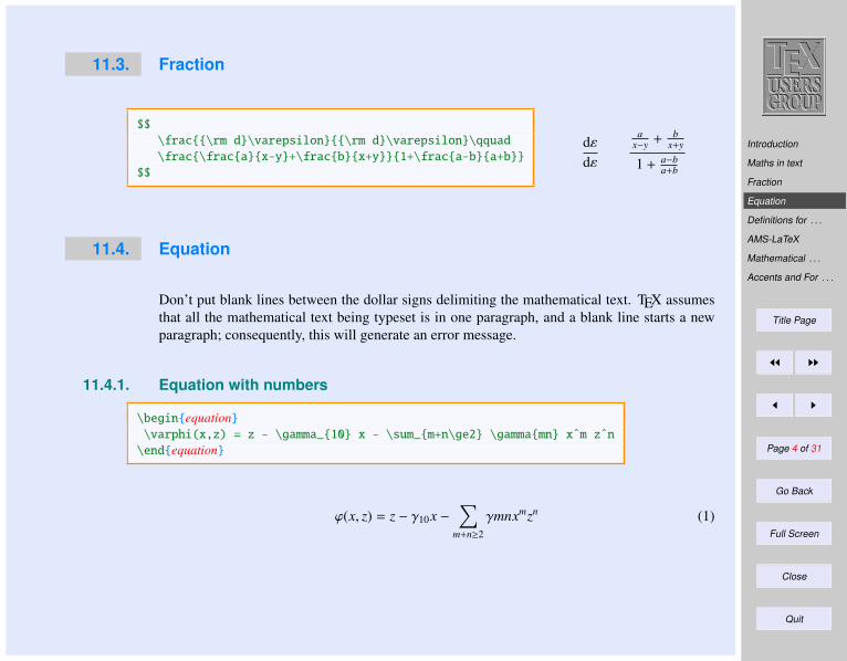
Introduction
Maths in text
Fraction
Equation
Definitions for . . .
AMS-LaTeX
Mathematical . . .
Accents and For . . .
Title Page
JJ II
J I
Page 4 of 31
Go Back
Full Screen
Close
Quit
11.3. Fraction
$$
\frac\rm d\varepsilon\rm d\varepsilon\qquad
\frac\fracax-y+\fracbx+y1+\fraca-ba+b
$$
dεdε
ax−y +
bx+y
1 + a−ba+b
11.4. Equation
Don’t put blank lines between the dollar signs delimiting the mathematical text. TEX assumesthat all the mathematical text being typeset is in one paragraph, and a blank line starts a newparagraph; consequently, this will generate an error message.
11.4.1. Equation with numbers
\beginequation\varphi(x,z) = z - \gamma_10 x - \sum_m+n\ge2 \gammamn xˆm zˆn
\endequation
ϕ(x, z) = z − γ10x −∑
m+n≥2
γmnxmzn (1)
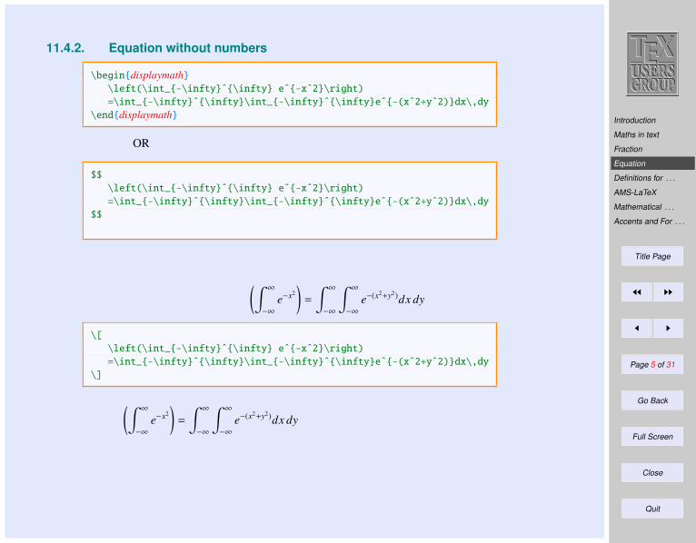
Introduction
Maths in text
Fraction
Equation
Definitions for . . .
AMS-LaTeX
Mathematical . . .
Accents and For . . .
Title Page
JJ II
J I
Page 5 of 31
Go Back
Full Screen
Close
Quit
11.4.2. Equation without numbers
\begindisplaymath\left(\int_-\inftyˆ\infty eˆ-xˆ2\right)
=\int_-\inftyˆ\infty\int_-\inftyˆ\inftyeˆ-(xˆ2+yˆ2)dx\,dy
\enddisplaymath
OR
$$
\left(\int_-\inftyˆ\infty eˆ-xˆ2\right)
=\int_-\inftyˆ\infty\int_-\inftyˆ\inftyeˆ-(xˆ2+yˆ2)dx\,dy
$$
(∫ ∞
−∞
e−x2)=
∫ ∞
−∞
∫ ∞
−∞
e−(x2+y2)dx dy
\[
\left(\int_-\inftyˆ\infty eˆ-xˆ2\right)
=\int_-\inftyˆ\infty\int_-\inftyˆ\inftyeˆ-(xˆ2+yˆ2)dx\,dy
\] (∫ ∞
−∞
e−x2)=
∫ ∞
−∞
∫ ∞
−∞
e−(x2+y2)dx dy
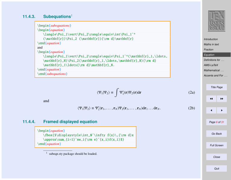
Introduction
Maths in text
Fraction
Equation
Definitions for . . .
AMS-LaTeX
Mathematical . . .
Accents and For . . .
Title Page
JJ II
J I
Page 6 of 31
Go Back
Full Screen
Close
Quit
11.4.3. Subequations1
\beginsubequations\beginequation
\langle\Psi_1\vert\Psi_2\rangle\equiv\int\Psi_1ˆ*
(\mathbfr)\Psi_2 (\mathbfr)\rm d\mathbfr
\endequationand\beginequation
\langle\Psi_1\vert\Psi_2\rangle\equiv\Psi_1ˆ*(\mathbfr_1,\ldots,
\mathbfr_N)\Psi_2(\mathbfr_1,\ldots,\mathbfr_N)\rm d
\mathbfr_1\ldots\rm d\mathbfr_N.
\endequation\endsubequations
〈Ψ1|Ψ2〉 ≡
∫Ψ∗1(r)Ψ2(r)dr (2a)
and
〈Ψ1|Ψ2〉 ≡ Ψ∗1(r1, . . . , rN)Ψ2(r1, . . . , rN)dr1 . . . drN . (2b)
11.4.4. Framed displayed equation
\beginequation\fbox$\displaystyle\int_0ˆ\infty f(x)\,\rm dx
\approx\sum_i=1ˆnw_i\rm eˆx_if(x_i)$
\endequation
1 subeqn.sty package should be loaded.
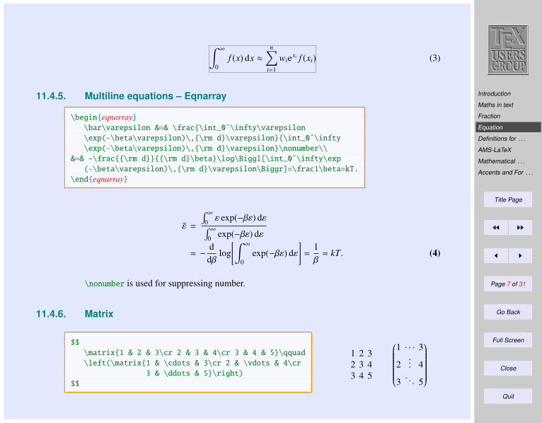
Introduction
Maths in text
Fraction
Equation
Definitions for . . .
AMS-LaTeX
Mathematical . . .
Accents and For . . .
Title Page
JJ II
J I
Page 7 of 31
Go Back
Full Screen
Close
Quit
∫ ∞
0f (x) dx ≈
n∑i=1
wiexi f (xi) (3)
11.4.5. Multiline equations – Eqnarray
\begineqnarray\bar\varepsilon &=& \frac\int_0ˆ\infty\varepsilon
\exp(-\beta\varepsilon)\,\rm d\varepsilon\int_0ˆ\infty
\exp(-\beta\varepsilon)\,\rm d\varepsilon\nonumber\\
&=& -\frac\rm d\rm d\beta\log\Biggl[\int_0ˆ\infty\exp
(-\beta\varepsilon)\,\rm d\varepsilon\Biggr]=\frac1\beta=kT.
\endeqnarray
ε =
∫ ∞0 ε exp(−βε) dε∫ ∞0 exp(−βε) dε
= −d
dβlog
[∫ ∞
0exp(−βε) dε
]=
1β= kT. (4)
\nonumber is used for suppressing number.
11.4.6. Matrix
$$
\matrix1 & 2 & 3\cr 2 & 3 & 4\cr 3 & 4 & 5\qquad
\left(\matrix1 & \cdots & 3\cr 2 & \vdots & 4\cr
3 & \ddots & 5\right)
$$
1 2 32 3 43 4 5
1 · · · 3
2... 4
3. . . 5
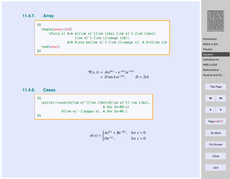
Introduction
Maths in text
Fraction
Equation
Definitions for . . .
AMS-LaTeX
Mathematical . . .
Accents and For . . .
Title Page
JJ II
J I
Page 8 of 31
Go Back
Full Screen
Close
Quit
11.4.7. Array
$$
\beginarraylcll\Psi(x,t) &=& A(\rm eˆ\rm ikx-\rm eˆ-\rm ikx)
\rm eˆ-\rm i\omega t&\\
&=& D\sin kx\rm eˆ-\rm i\omega t, & D=2\rm iA
\endarray$$
Ψ(x, t) = A(eikx − e−ikx)e−iωt
= D sin kxe−iωt, D = 2iA
11.4.8. Cases
$$
\psi(x)=\casesA\rm eˆ\rm ikx+B\rm eˆ-\rm ikx,
& for $x=0$\cr
D\rm eˆ-\kappa x, & for $x=0$.
$$
ψ(x) =
Aeikx + Be−ikx, for x = 0De−κx, for x = 0.
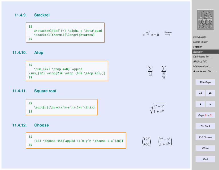
Introduction
Maths in text
Fraction
Equation
Definitions for . . .
AMS-LaTeX
Mathematical . . .
Accents and For . . .
Title Page
JJ II
J I
Page 9 of 31
Go Back
Full Screen
Close
Quit
11.4.9. Stackrel
$$
a\stackreldef= \alpha + \beta\quad
\stackrelthermo\longrightarrow
$$
ade f= α + β
thermo−→
11.4.10. Atop
$$
\sum_k=1 \atop k=0 \qquad
\sum_123 \atop234 \atop 890 \atop 456
$$
∑k=1k=0
∑123234890456
11.4.11. Square root
$$
\sqrt[n]\fracxˆn-yˆn1+uˆ2n
$$
n
√xn − yn
1 + u2n
11.4.12. Choose
$$
123 \choose 456\qquad xˆn-yˆn \choose 1+uˆ2n
$$
(123456
) (xn − yn
1 + u2n
)

Introduction
Maths in text
Fraction
Equation
Definitions for . . .
AMS-LaTeX
Mathematical . . .
Accents and For . . .
Title Page
JJ II
J I
Page 10 of 31
Go Back
Full Screen
Close
Quit
11.5. Definitions for Theorems
We should define \newtheoremthmTheorem etc in preamble.
\newtheoremthmTheorem
\beginthm
This is body matter for testing this environment.
\endthm
Theorem 1 This is body matterfor testing this environment.
\newtheoremrmkRemark[section]\beginrmkThis is body matter for testing this environment.
\endrmk
Remark 11.5.1 This is bodymatter for testing this environ-ment.
\newtheoremcolCorollary\begincol[Richard, 1987]This is body matter for testing this environment.
\endcol
Corollary 1 (Richard, 1987)This is body matter for testingthis environment.
\newtheoremlemLemma[thm]
\beginlem
This is body matter for testing this environment.
\endlem
Lemma 1.1 This is body matterfor testing this environment.
\newtheoremexaExample[lem]
\beginexaThis is body matter for testing this environment.
\endexa
Example 1.1.1 This is body mat-ter for testing this environment.
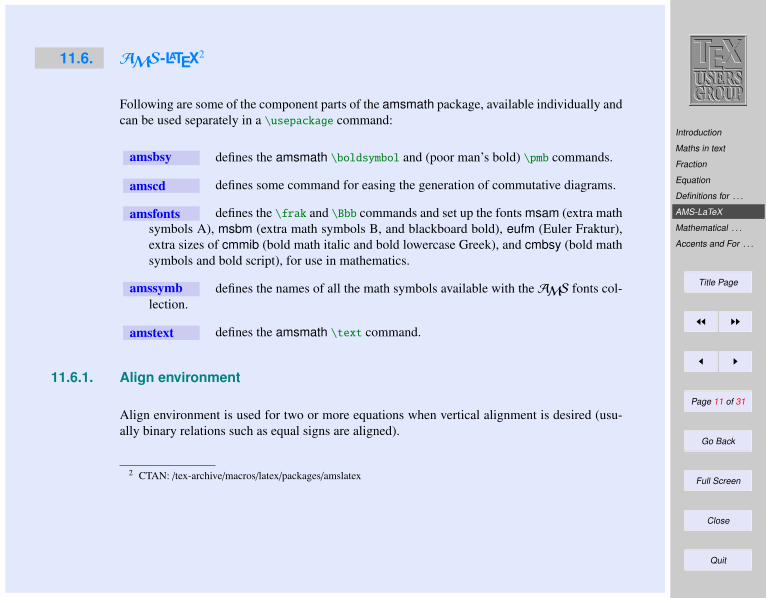
Introduction
Maths in text
Fraction
Equation
Definitions for . . .
AMS-LaTeX
Mathematical . . .
Accents and For . . .
Title Page
JJ II
J I
Page 11 of 31
Go Back
Full Screen
Close
Quit
11.6. AMS-LATEX2
Following are some of the component parts of the amsmath package, available individually andcan be used separately in a \usepackage command:
amsbsy defines the amsmath \boldsymbol and (poor man’s bold) \pmb commands.
amscd defines some command for easing the generation of commutative diagrams.
amsfonts defines the \frak and \Bbb commands and set up the fonts msam (extra mathsymbols A), msbm (extra math symbols B, and blackboard bold), eufm (Euler Fraktur),extra sizes of cmmib (bold math italic and bold lowercase Greek), and cmbsy (bold mathsymbols and bold script), for use in mathematics.
amssymb defines the names of all the math symbols available with theAMS fonts col-lection.
amstext defines the amsmath \text command.
11.6.1. Align environment
Align environment is used for two or more equations when vertical alignment is desired (usu-ally binary relations such as equal signs are aligned).
2 CTAN: /tex-archive/macros/latex/packages/amslatex
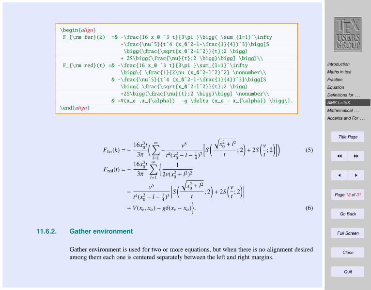
Introduction
Maths in text
Fraction
Equation
Definitions for . . .
AMS-LaTeX
Mathematical . . .
Accents and For . . .
Title Page
JJ II
J I
Page 12 of 31
Go Back
Full Screen
Close
Quit
\beginalignF_\rm fer(k) =& -\frac16 x_0 ˆ3 t3\pi \bigg( \sum_l=1ˆ\infty
-\frac\nuˆ5tˆ4 (x_0ˆ2-l-\frac14)ˆ3\bigg[S
\bigg(\frac\sqrtx_0ˆ2+lˆ2t;2 \bigg)
+ 2S\bigg(\frac\nut;2 \bigg)\bigg] \bigg)\\
F_\rm red(t) =& -\frac16 x_0 ˆ3 t3\pi \sum_l=1ˆ\infty
\bigg\ \frac12\nu (x_0ˆ2+lˆ2)ˆ2 \nonumber\\
& -\frac\nuˆ5tˆ4 (x_0ˆ2-l-\frac14)ˆ3\bigg[S
\bigg( \frac\sqrtx_0ˆ2+lˆ2t;2 \bigg)
+2S\bigg(\frac\nut;2 \bigg)\bigg] \nonumber\\
& +V(x_e ,x_\alpha) -g \delta (x_e - x_\alpha) \bigg\.
\endalign
Ffer(k) = −16x3
0t3π
( ∞∑l=1
−ν5
t4(x20 − l − 1
4 )3
[S( √
x20 + l2
t; 2
)+ 2S
(ν
t; 2
)])(5)
Fred(t) = −16x3
0t3π
∞∑l=1
12ν(x2
0 + l2)2
−ν5
t4(x20 − l − 1
4 )3
[S( √
x20 + l2
t; 2
)+ 2S
(ν
t; 2
)]+ V(xe, xα) − gδ(xe − xα)
. (6)
11.6.2. Gather environment
Gather environment is used for two or more equations, but when there is no alignment desiredamong them each one is centered separately between the left and right margins.
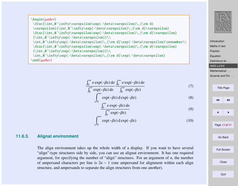
Introduction
Maths in text
Fraction
Equation
Definitions for . . .
AMS-LaTeX
Mathematical . . .
Accents and For . . .
Title Page
JJ II
J I
Page 13 of 31
Go Back
Full Screen
Close
Quit
\begingather\frac\int_0ˆ\infty\varepsilon\exp(-\beta\varepsilon)\,\rm d
\varepsilon\int_0ˆ\infty\exp(-\beta\varepsilon)\,\rm d\varepsilon
\frac\int_0ˆ\infty\varepsilon\exp(-\beta\varepsilon)\,\rm d\varepsilon
\int_0ˆ\infty\exp(-\beta\varepsilon)\\
\int_0ˆ\infty\exp(-\beta\varepsilon)\,\rm d\exp(-\beta\varepsilon)\nonumber\\
\frac\int_0ˆ\infty\varepsilon\exp(-\beta\varepsilon)\,\rm d\varepsilon
\int_0ˆ\infty\exp(-\beta\varepsilon)\\
\int_0ˆ\infty\exp(-\beta\varepsilon)\,\rm d\exp(-\beta\varepsilon)
\endgather
∫ ∞0 ε exp(−βε) dε∫ ∞0 exp(−βε) dε
∫ ∞0 ε exp(−βε) dε∫ ∞
0 exp(−βε)(7)∫ ∞
0exp(−βε) d exp(−βε) (8)∫ ∞0 ε exp(−βε) dε∫ ∞
0 exp(−βε)(9)∫ ∞
0exp(−βε) d exp(−βε) (10)
11.6.3. Alignat environment
The align environment takes up the whole width of a display. If you want to have several“align”-type structures side by side, you can use an alignat environment. It has one requiredargument, for specifying the number of “align” structures. For an argument of n, the numberof ampersand characters per line is 2n − 1 (one ampersand for alignment within each alignstructure, and ampersands to separate the align structures from one another).
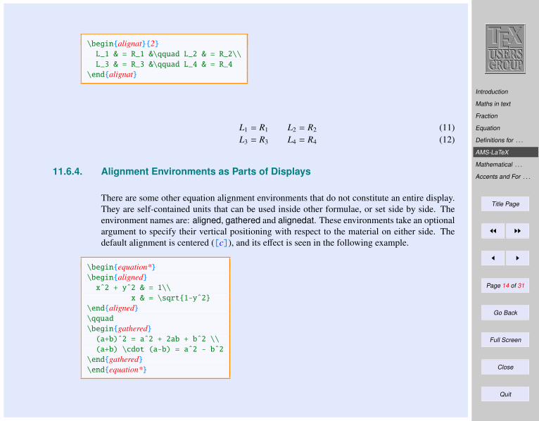
Introduction
Maths in text
Fraction
Equation
Definitions for . . .
AMS-LaTeX
Mathematical . . .
Accents and For . . .
Title Page
JJ II
J I
Page 14 of 31
Go Back
Full Screen
Close
Quit
\beginalignat2L_1 & = R_1 &\qquad L_2 & = R_2\\
L_3 & = R_3 &\qquad L_4 & = R_4
\endalignat
L1 = R1 L2 = R2 (11)L3 = R3 L4 = R4 (12)
11.6.4. Alignment Environments as Parts of Displays
There are some other equation alignment environments that do not constitute an entire display.They are self-contained units that can be used inside other formulae, or set side by side. Theenvironment names are: aligned, gathered and alignedat. These environments take an optionalargument to specify their vertical positioning with respect to the material on either side. Thedefault alignment is centered ([c]), and its effect is seen in the following example.
\beginequation*\beginalignedxˆ2 + yˆ2 & = 1\\
x & = \sqrt1-yˆ2
\endaligned\qquad
\begingathered(a+b)ˆ2 = aˆ2 + 2ab + bˆ2 \\
(a+b) \cdot (a-b) = aˆ2 - bˆ2
\endgathered\endequation*

Introduction
Maths in text
Fraction
Equation
Definitions for . . .
AMS-LaTeX
Mathematical . . .
Accents and For . . .
Title Page
JJ II
J I
Page 15 of 31
Go Back
Full Screen
Close
Quit
x2 + y2 = 1
x =√
1 − y2
(a + b)2 = a2 + 2ab + b2
(a + b) · (a − b) = a2 − b2
The same mathematics can now be typeset using vertical alignments for the environments.
\beginequation*\beginaligned[b]xˆ2 + yˆ2 & = 1\\
x & = \sqrt1-yˆ2
\endaligned\qquad
\begingathered[t](a+b)ˆ2 = aˆ2 + 2ab + bˆ2 \\
(a+b) \cdot (a-b) = aˆ2 - bˆ2
\endgathered\endequation*
x2 + y2 = 1
x =√
1 − y2 (a + b)2 = a2 + 2ab + b2
(a + b) · (a − b) = a2 − b2
11.6.5. Multline environment
The multline environment is a variation of the equation environment used for equations that donot fit on a single line. The first line of a multline will be at the left margin and the last line atthe right margin except for an indentation on both sides whose amount is equal to multline-gap.
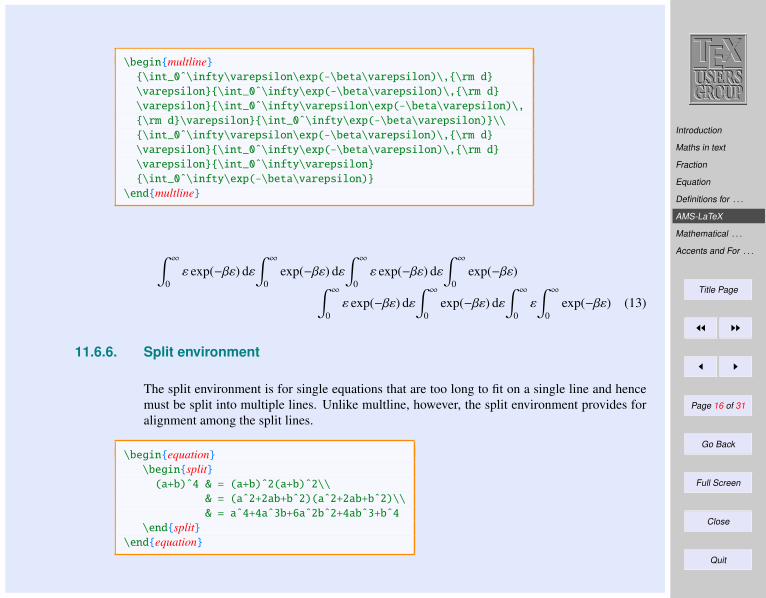
Introduction
Maths in text
Fraction
Equation
Definitions for . . .
AMS-LaTeX
Mathematical . . .
Accents and For . . .
Title Page
JJ II
J I
Page 16 of 31
Go Back
Full Screen
Close
Quit
\beginmultline\int_0ˆ\infty\varepsilon\exp(-\beta\varepsilon)\,\rm d
\varepsilon\int_0ˆ\infty\exp(-\beta\varepsilon)\,\rm d
\varepsilon\int_0ˆ\infty\varepsilon\exp(-\beta\varepsilon)\,
\rm d\varepsilon\int_0ˆ\infty\exp(-\beta\varepsilon)\\
\int_0ˆ\infty\varepsilon\exp(-\beta\varepsilon)\,\rm d
\varepsilon\int_0ˆ\infty\exp(-\beta\varepsilon)\,\rm d
\varepsilon\int_0ˆ\infty\varepsilon
\int_0ˆ\infty\exp(-\beta\varepsilon)
\endmultline
∫ ∞
0ε exp(−βε) dε
∫ ∞
0exp(−βε) dε
∫ ∞
0ε exp(−βε) dε
∫ ∞
0exp(−βε)∫ ∞
0ε exp(−βε) dε
∫ ∞
0exp(−βε) dε
∫ ∞
0ε
∫ ∞
0exp(−βε) (13)
11.6.6. Split environment
The split environment is for single equations that are too long to fit on a single line and hencemust be split into multiple lines. Unlike multline, however, the split environment provides foralignment among the split lines.
\beginequation\beginsplit(a+b)ˆ4 & = (a+b)ˆ2(a+b)ˆ2\\
& = (aˆ2+2ab+bˆ2)(aˆ2+2ab+bˆ2)\\
& = aˆ4+4aˆ3b+6aˆ2bˆ2+4abˆ3+bˆ4
\endsplit\endequation
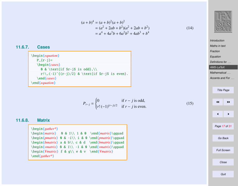
Introduction
Maths in text
Fraction
Equation
Definitions for . . .
AMS-LaTeX
Mathematical . . .
Accents and For . . .
Title Page
JJ II
J I
Page 17 of 31
Go Back
Full Screen
Close
Quit
(a + b)4 = (a + b)2(a + b)2
= (a2 + 2ab + b2)(a2 + 2ab + b2)= a4 + 4a3b + 6a2b2 + 4ab3 + b4
(14)
11.6.7. Cases
\beginequationP_r-j=
\begincases0 & \textif $r-j$ is odd,\\
r!\,(-1)ˆ(r-j)/2 & \textif $r-j$ is even.
\endcases\endequation
Pr− j =
0 if r − j is odd,r! (−1)(r− j)/2 if r − j is even.
(15)
11.6.8. Matrix
\begingather*\beginmatrix 0 & 1\\ 1 & 0 \endmatrix\qquad\beginpmatrix 0 & -i\\ i & 0 \endpmatrix\qquad\beginbmatrix a & b\\ c & d \endbmatrix\qquad\beginvmatrix 0 & 1\\ -1 & 0 \endvmatrix\qquad\beginVmatrix f & g\\ e & v \endVmatrix\endgather*
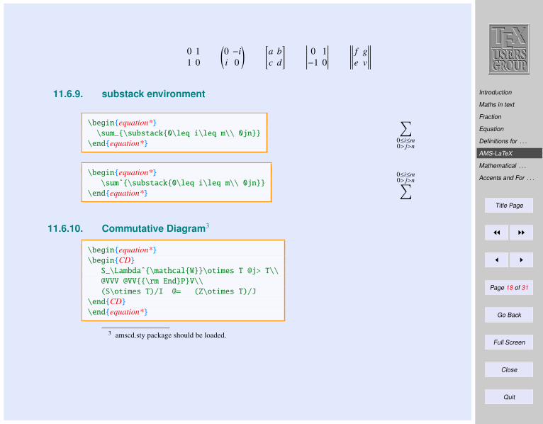
Introduction
Maths in text
Fraction
Equation
Definitions for . . .
AMS-LaTeX
Mathematical . . .
Accents and For . . .
Title Page
JJ II
J I
Page 18 of 31
Go Back
Full Screen
Close
Quit
0 11 0
(0 −ii 0
) [a bc d
] ∣∣∣∣∣∣ 0 1−1 0
∣∣∣∣∣∣ ∥∥∥∥∥∥ f ge v
∥∥∥∥∥∥11.6.9. substack environment
\beginequation*\sum_\substack0\leq i\leq m\\ 0jn
\endequation*
∑0≤i≤m0> j>n
\beginequation*\sumˆ\substack0\leq i\leq m\\ 0jn
\endequation*
0≤i≤m0> j>n∑
11.6.10. Commutative Diagram3
\beginequation*\beginCD
S_\Lambdaˆ\mathcalW\otimes T @j> T\\
@VVV @VV\rm EndPV\\
(S\otimes T)/I @= (Z\otimes T)/J
\endCD
\endequation*
3 amscd.sty package should be loaded.

Introduction
Maths in text
Fraction
Equation
Definitions for . . .
AMS-LaTeX
Mathematical . . .
Accents and For . . .
Title Page
JJ II
J I
Page 19 of 31
Go Back
Full Screen
Close
Quit
SWΛ⊗ T
j−−−−−→ Ty yEndP
(S ⊗ T )/I (Z ⊗ T )/J
\beginequation*\beginCD
S_\Lambdaˆ\mathcalW\otimes T @j> T_XF @xyz> T\\
@VOutpVV & & @AA\rm EndPA\\
(S\otimes T)/I @= X_\mathcalF @fg> (Z\otimes T)/J
\endCD
\endequation*
SWΛ⊗ T
j−−−−−→ TXF
xyz−−−−−→ T
Outpy xEndP
(S ⊗ T )/I XFf g
−−−−−→ (Z ⊗ T )/J
11.6.11. Binom
\beginequation*\binomxy
\endequation*
(xy
)11.6.12. AMS symbols
\iint!
\iiint#
\iiiint%
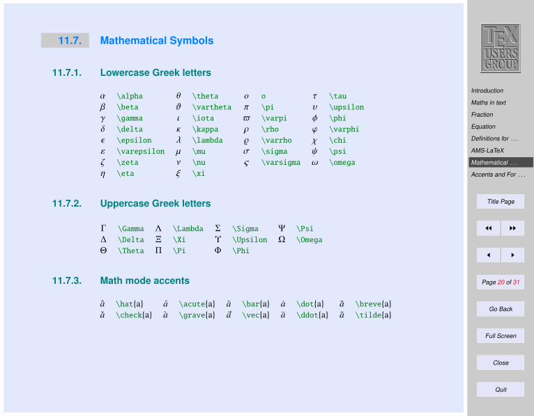
Introduction
Maths in text
Fraction
Equation
Definitions for . . .
AMS-LaTeX
Mathematical . . .
Accents and For . . .
Title Page
JJ II
J I
Page 20 of 31
Go Back
Full Screen
Close
Quit
11.7. Mathematical Symbols
11.7.1. Lowercase Greek letters
α \alpha θ \theta o o τ \tau
β \beta ϑ \vartheta π \pi υ \upsilon
γ \gamma ι \iota $ \varpi φ \phi
δ \delta κ \kappa ρ \rho ϕ \varphi
ε \epsilon λ \lambda % \varrho χ \chi
ε \varepsilon µ \mu σ \sigma ψ \psi
ζ \zeta ν \nu ς \varsigma ω \omega
η \eta ξ \xi
11.7.2. Uppercase Greek letters
Γ \Gamma Λ \Lambda Σ \Sigma Ψ \Psi
∆ \Delta Ξ \Xi Υ \Upsilon Ω \Omega
Θ \Theta Π \Pi Φ \Phi
11.7.3. Math mode accents
a \hata a \acutea a \bara a \dota a \breveaa \checka a \gravea ~a \veca a \ddota a \tildea
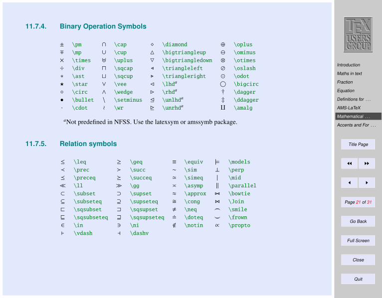
Introduction
Maths in text
Fraction
Equation
Definitions for . . .
AMS-LaTeX
Mathematical . . .
Accents and For . . .
Title Page
JJ II
J I
Page 21 of 31
Go Back
Full Screen
Close
Quit
11.7.4. Binary Operation Symbols
± \pm ∩ \cap \diamond ⊕ \oplus
∓ \mp ∪ \cup 4 \bigtriangleup \ominus
× \times ] \uplus 5 \bigtriangledown ⊗ \otimes
÷ \div u \sqcap / \triangleleft \oslash
∗ \ast t \sqcup . \triangleright \odot
? \star ∨ \vee C \lhda © \bigcirc
\circ ∧ \wedge B \rhda † \dagger
• \bullet \ \setminus E \unlhda ‡ \ddagger
· \cdot o \wr D \unrhda q \amalg
aNot predefined in NFSS. Use the latexsym or amssymb package.
11.7.5. Relation symbols
≤ \leq ≥ \geq ≡ \equiv |= \models
≺ \prec \succ ∼ \sim ⊥ \perp
\preceq \succeq ' \simeq | \mid
\ll \gg \asymp ‖ \parallel
⊂ \subset ⊃ \supset ≈ \approx ./ \bowtie
⊆ \subseteq ⊇ \supseteq \cong Z \Join
@ \sqsubset A \sqsupset , \neq ^ \smile
v \sqsubseteq w \sqsupseteq \doteq _ \frown
∈ \in 3 \ni < \notin ∝ \propto
` \vdash a \dashv
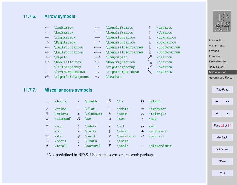
Introduction
Maths in text
Fraction
Equation
Definitions for . . .
AMS-LaTeX
Mathematical . . .
Accents and For . . .
Title Page
JJ II
J I
Page 22 of 31
Go Back
Full Screen
Close
Quit
11.7.6. Arrow symbols
← \leftarrow ←− \longleftarrow ↑ \uparrow
⇐ \Leftarrow ⇐= \Longleftarrow ⇑ \Uparrow
→ \rightarrow −→ \longrightarrow ↓ \downarrow
⇒ \Rightarrow =⇒ \Longrightarrow ⇓ \Downarrow
↔ \leftrightarrow ←→ \longleftrightarrow l \updownarrow
⇔ \Leftrightarrow ⇐⇒ \Longleftrightarrow m \Updownarrow
7→| \mapsto 7−→ \longmapsto \nearrow
← \hookleftarrow → \hookrightarrow \searrow
\leftharpoonup \rightharpoonup \swarrow
\leftharpoondown \rightharpoondown \nwarrow
\rightleftharpoons \leadsto
11.7.7. Miscellaneous symbols
. . . \ldots ı \imath = \Im ℵ \aleph
′ \prime [ \flat. . . \ddots ∅ \emptyset
∃ \exists ♣ \clubsuit ~ \hbar 4 \triangle
^ \Diamonda < \Re \Boxa , \neq
> \top... \vdots ` \ell ℘ \wp
⊥ \bot ∞ \infty ] \sharp ♠ \spadesuit
f \mho√
\surd ♥ \heartsuit ∂ \partial
· · · \cdots \jmath ∠ \angle
∀ \forall \ \natural ∇ \nabla ♦ \diamondsuit
aNot predefined in NFSS. Use the latexsym or amssymb package.
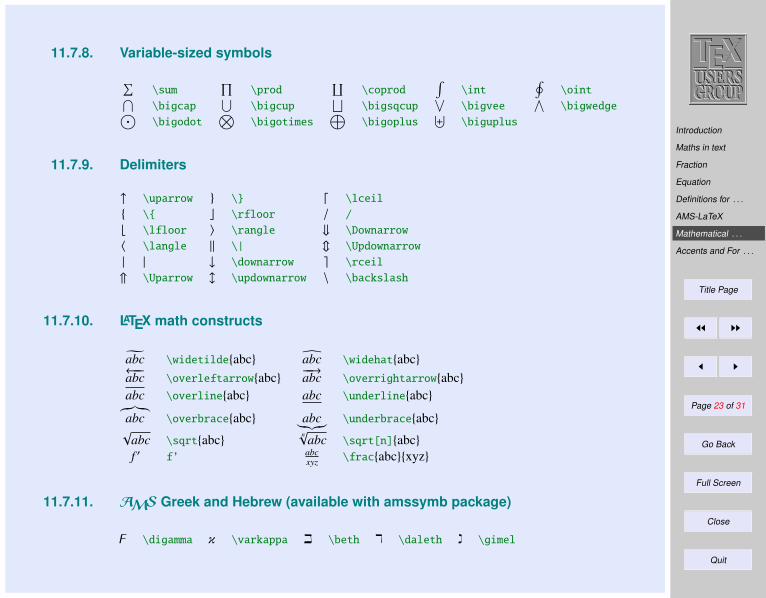
Introduction
Maths in text
Fraction
Equation
Definitions for . . .
AMS-LaTeX
Mathematical . . .
Accents and For . . .
Title Page
JJ II
J I
Page 23 of 31
Go Back
Full Screen
Close
Quit
11.7.8. Variable-sized symbols∑\sum
∏\prod
∐\coprod
∫\int
∮\oint⋂
\bigcap⋃
\bigcup⊔
\bigsqcup∨
\bigvee∧
\bigwedge⊙\bigodot
⊗\bigotimes
⊕\bigoplus
⊎\biguplus
11.7.9. Delimiters
↑ \uparrow \ d \lceil
\ c \rfloor / /
b \lfloor 〉 \rangle ⇓ \Downarrow
〈 \langle ‖ \| m \Updownarrow
| | ↓ \downarrow e \rceil
⇑ \Uparrow l \updownarrow \ \backslash
11.7.10. LATEX math constructs
abc \widetildeabc abc \widehatabc←−−abc \overleftarrowabc −−→abc \overrightarrowabcabc \overlineabc abc \underlineabc︷︸︸︷abc \overbraceabc abc︸︷︷︸ \underbraceabc√
abc \sqrtabc n√abc \sqrt[n]abcf ′ f’ abc
xyz \fracabcxyz
11.7.11. AMS Greek and Hebrew (available with amssymb package)
z \digamma κ \varkappa i \beth k \daleth ג \gimel
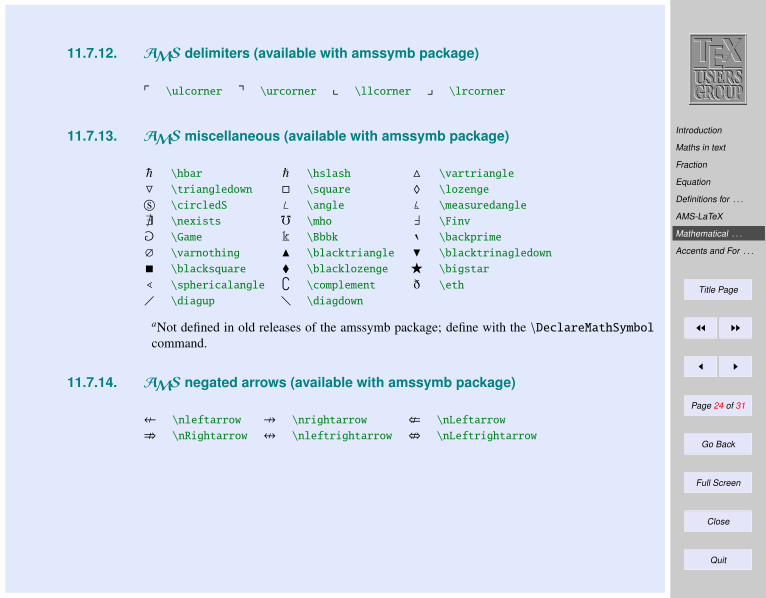
Introduction
Maths in text
Fraction
Equation
Definitions for . . .
AMS-LaTeX
Mathematical . . .
Accents and For . . .
Title Page
JJ II
J I
Page 24 of 31
Go Back
Full Screen
Close
Quit
11.7.12. AMS delimiters (available with amssymb package)
p \ulcorner q \urcorner x \llcorner y \lrcorner
11.7.13. AMS miscellaneous (available with amssymb package)
~ \hbar \hslash M \vartriangle
O \triangledown \square ♦ \lozenge
s \circledS ∠ \angle ] \measuredangle
@ \nexists f \mho ` \Finv
a \Game k \Bbbk 8 \backprime
∅ \varnothing N \blacktriangle H \blacktrinagledown
\blacksquare \blacklozenge F \bigstar
^ \sphericalangle \complement ð \eth
\diagup \diagdown
aNot defined in old releases of the amssymb package; define with the \DeclareMathSymbolcommand.
11.7.14. AMS negated arrows (available with amssymb package)
8 \nleftarrow 9 \nrightarrow : \nLeftarrow
; \nRightarrow = \nleftrightarrow < \nLeftrightarrow
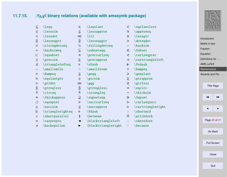
Introduction
Maths in text
Fraction
Equation
Definitions for . . .
AMS-LaTeX
Mathematical . . .
Accents and For . . .
Title Page
JJ II
J I
Page 25 of 31
Go Back
Full Screen
Close
Quit
11.7.15. AMS binary relations (available with amssymb package)
5 \leqq 6 \leqslant 0 \eqslantless
. \lesssim / \lessapprox u \approxeq
l \lessdot ≪ \lll ≶ \lessgtr
Q \lesseqgtr S \lesseqqgtr + \doteqdot
: \risingdotseq ; \fallingdotseq v \backsim
w \backsimeq j \subseteqq b \Subset
@ \sqsubset 4 \preccurlyeq 2 \curlyeqprec
- \precsim w \precapprox C \vartriangleleft
E \trianglelefteq \vDash \Vvdash
` \smallsmile a \smallfrown l \bumpeq
m \Bumpeq = \geqq > \geqslant
1 \eqslantgtr & \gtrsim ' \gtrapprox
m \gtrdot ≫ \ggg ≷ \gtrless
R \gtreqless T \gtreqqless P \eqcirc
$ \circeq , \triangleq ∼ \thicksim
≈ \thickapprox k \supseteqq c \Supset
A \sqsupset < \succcurlyeq 3 \curlyeqsucc
% \succsim v \succapprox B \vartriangleright
D \trianglerighteq \Vdash p \shortmid
q \shortparallel G \between t \pitchfork
∝ \varpropto J \blacktriangleleft ∴ \therefore
\backepsilon I \blacktriangleright ∵ \because
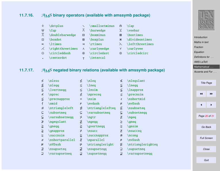
Introduction
Maths in text
Fraction
Equation
Definitions for . . .
AMS-LaTeX
Mathematical . . .
Accents and For . . .
Title Page
JJ II
J I
Page 26 of 31
Go Back
Full Screen
Close
Quit
11.7.16. AMS binary operators (available with amssymb package)
u \dotplus r \smallsetminus e \Cap
d \Cup Z \barwedge Y \veebar
[ \doublebarwedge \boxminus \boxtimes
\boxdot \boxplus > \divideontimes
n \ltimes o \rtimes h \leftthreetimes
i \rightthreetimes f \curlywedge g \curlyvee
\circleddash ~ \circledast \circledcirc
\centerdot ᵀ \intercal
11.7.17. AMS negated binary relations (available with amssymb package)
≮ \nless \nleq \nleqslant
\nleqq \lneq \lneqq
\lvertneqq \lnsim \lnapprox
⊀ \nprec \npreceq \precnsim
\precnapprox / \nsim . \nshortmid
- \nmid 0 \nvdash 2 \nvDash
6 \ntriangleleft 5 \ntrianglelefteq * \nsubseteq
( \subsetneq \varsubsetneq $ \subsetneqq
& \varsubsetneqq ≯ \ngtr \ngeq
\ngeqslant \ngeqq \gneq
\gneqq \gvertneqq \gnsim
\gnapprox \nsucc \nsucceq
\succnsim \succnapprox \ncong
/ \nshortparallel ∦ \nparallel 2 \nvDash
3 \nVDash 7 \ntriangleright 4 \ntrianglerighteq
+ \nsupseteq # \nsupseteqq ) \supsetneq
! \varsupsetneq % \supsetneqq ' \varsupsetneqq
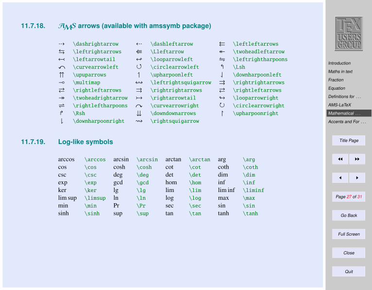
Introduction
Maths in text
Fraction
Equation
Definitions for . . .
AMS-LaTeX
Mathematical . . .
Accents and For . . .
Title Page
JJ II
J I
Page 27 of 31
Go Back
Full Screen
Close
Quit
11.7.18. AMS arrows (available with amssymb package)
d \dashrightarrow c \dashleftarrow ⇔ \leftleftarrows
\leftrightarrows W \Lleftarrow \twoheadleftarrow
\leftarrowtail " \looparrowleft \leftrightharpoons
x \curvearrowleft \circlearrowleft \Lsh
\upuparrows \upharpoonleft \downharpoonleft
( \multimap ! \leftrightsquigarrow ⇒ \rightrightarrows
\rightleftarrows ⇒ \rightrightarrows \rightleftarrows
\twoheadrightarrow \rightarrowtail # \looparrowright
\rightleftharpoons y \curvearrowright \circlearrowright
\Rsh \downdownarrows \upharpoonright
\downharpoonright \rightsquigarrow
11.7.19. Log-like symbols
arccos \arccos arcsin \arcsin arctan \arctan arg \arg
cos \cos cosh \cosh cot \cot coth \coth
csc \csc deg \deg det \det dim \dim
exp \exp gcd \gcd hom \hom inf \inf
ker \ker lg \lg lim \lim lim inf \liminf
lim sup \limsup ln \ln log \log max \max
min \min Pr \Pr sec \sec sin \sin
sinh \sinh sup \sup tan \tan tanh \tanh
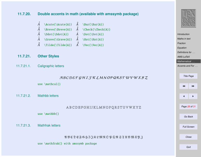
Introduction
Maths in text
Fraction
Equation
Definitions for . . .
AMS-LaTeX
Mathematical . . .
Accents and For . . .
Title Page
JJ II
J I
Page 28 of 31
Go Back
Full Screen
Close
Quit
11.7.20. Double accents in math (available with amssymb package)
´A \Acute\AcuteA ¯A \Bar\BarA˘A \Breve\BreveA
ˇA \Check\CheckA¨A \Ddot\DdotA ˙A \Dot\DotA`A \Grave\GraveA
ˆA \Hat\HatA
˜A \Tilde\TildeA~~A \Vec\VecA
11.7.21. Other Styles
11.7.21.1. Caligraphic letters
ABCDEF GH IJ K LMN OPQRST UVWXYZ
use \mathcal
11.7.21.2. Mathbb letters
ABCDEFGH I JKLMNOPQRSTUVWXYZ
use \mathbb
11.7.21.3. Mathfrak letters
ABCDEFGHIJKLMNOPQRSTUVWXYZ
use \mathfrak with amssymb package
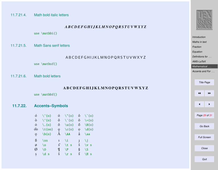
Introduction
Maths in text
Fraction
Equation
Definitions for . . .
AMS-LaTeX
Mathematical . . .
Accents and For . . .
Title Page
JJ II
J I
Page 29 of 31
Go Back
Full Screen
Close
Quit
11.7.21.4. Math bold italic letters
A B C D E F G H I J K L M N O P Q R S T U V W X Y Z
use \mathbi
11.7.21.5. Math Sans serif letters
A BC D E F GH I J KL M NO P Q RS TU V W X Y Z
use \mathsf
11.7.21.6. Math bold letters
A B C D E F G H I J K L M N O P Q R S T U V W X Y Z
use \mathbf
11.7.22. Accents–Symbols
o \’o o \"o o \ˆo
o \‘o o \˜o o \=o
o \.o o \uo o \Ho
oo \too o \co o. \do
o¯
\bo Å \AA å \aa
ß \ss ı \i \j
ø \o s \t s s \v s
Ø \O ¶ \P § \S
s. \d s s \r s s \H s
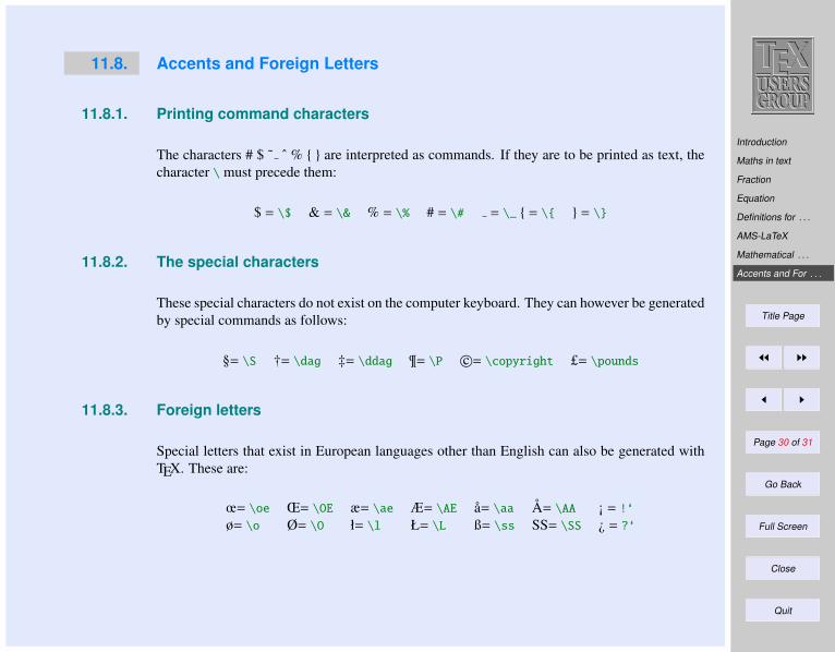
Introduction
Maths in text
Fraction
Equation
Definitions for . . .
AMS-LaTeX
Mathematical . . .
Accents and For . . .
Title Page
JJ II
J I
Page 30 of 31
Go Back
Full Screen
Close
Quit
11.8. Accents and Foreign Letters
11.8.1. Printing command characters
The characters # $ ˜ ˆ % are interpreted as commands. If they are to be printed as text, thecharacter \ must precede them:
$ = \$ & = \& % = \% # = \# = \_ = \ = \
11.8.2. The special characters
These special characters do not exist on the computer keyboard. They can however be generatedby special commands as follows:
§= \S †= \dag ‡= \ddag ¶= \P c©= \copyright £= \pounds
11.8.3. Foreign letters
Special letters that exist in European languages other than English can also be generated withTEX. These are:
œ= \oe Œ= \OE æ= \ae Æ= \AE å= \aa Å= \AA ¡ = !‘
ø= \o Ø= \O ł= \l Ł= \L ß= \ss SS= \SS ¿ = ?‘
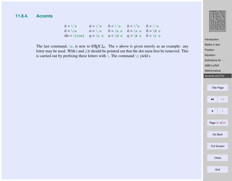
Introduction
Maths in text
Fraction
Equation
Definitions for . . .
AMS-LaTeX
Mathematical . . .
Accents and For . . .
Title Page
JJ II
J I
Page 31 of 31
Go Back
Full Screen
Close
Quit
11.8.4. Accents
o = \‘o o = \’o o = \ˆo o = \"o o = \˜o
o = \=o o = \.o o = \u o o = \v o o = \H o
oo = \too o = \c o o. = \d o o¯= \b o o = \r o
The last command, \r, is new to LATEX 2ε. The o above is given merely as an example: anyletter may be used. With i and j it should be pointed out that the dot must first be removed. Thisis carried out by prefixing these letters with \. The command \i yield ı.
Why cross refer . . .
Let LATEX do it
Pointing to a . . .
Pointing outside . . .
Lost the keys? . . .
Title Page
JJ II
J I
Page 1 of 16
Go Back
Full Screen
Close
Quit
Indian TEX Users Group: http://www.river-valley.com/tug
12On-line Tutorial on LATEX
The Tutorial TeamIndian TEX Users Group, Buildings, Cotton Hills
Trivandrum 695014, 2000
Prof. (Dr.) K. S. S. Nambooripad, Director, Center for Mathematical Sciences, Trivandrum, (Editor); Dr. E. Krishnan, Readerin Mathematics, University College, Trivandrum; Mohit Agarwal, Department of Aerospace Engineering, Indian Institute of
Science, Bangalore; T. Rishi, Focal Image (India) Pvt. Ltd., Trivandrum; L. A. Ajith, Focal Image (India) Pvt. Ltd.,Trivandrum; A. M. Shan, Focal Image (India) Pvt. Ltd., Trivandrum; C. V. Radhakrishnan, River Valley Technologies,
Software Technology Park, Trivandrum constitute the Tutorial team
This document is generated from LATEX sources compiled with pdfLATEX v. 14e in an INTEL
Pentium III 700 MHz system running Linux kernel version 2.2.14-12. The packages usedare hyperref.sty and pdfscreen.sty
c©2000, Indian TEX Users Group. This document may be distributed under the terms of the LATEXProject Public License, as described in lppl.txt in the base LATEX distribution, either version 1.0
or, at your option, any later version
Why cross refer . . .
Let LATEX do it
Pointing to a . . .
Pointing outside . . .
Lost the keys? . . .
Title Page
JJ II
J I
Page 2 of 16
Go Back
Full Screen
Close
Quit
12 Cross References in LATEX
12.1. Why cross references?
Cross reference is the technical term for quoting yourself. This is what you do when you saysomething like, “As I said earlier, . . . ”. More seriously, in a written article, you may often haveoccasion to refer the reader to something mentioned earlier (or sometimes to something yet tobe said) in the same document. Thus you may have explained a new term in the second sectionof your article and when you use this term again in the fourth section, it is a matter of courtesyto the reader to point to the explanation. Again, in a Mathematics article, you may have to citean earlier result in the proof of the current result.
Such references can be done by hand, but if you revise your document and insert some newsections (or theorems) then changing all cross references manually is no easy task. It is alwaysbetter to automate such tedious tasks.(After all what’s a computer for, if not to do such mundanejobs?)
12.2. Let LATEX do it
The basic method of using cross references (see Section 12.1 for what we mean by cross referee)in LATEX is quite simple. Suppose that somewhere in the in the second section of you article,you want to refer to the first section. You assign a key to the first section using the command
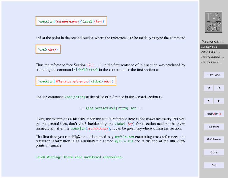
Why cross refer . . .
Let LATEX do it
Pointing to a . . .
Pointing outside . . .
Lost the keys? . . .
Title Page
JJ II
J I
Page 3 of 16
Go Back
Full Screen
Close
Quit
\section〈section name〉\label〈key〉
and at the point in the second section where the reference is to be made, you type the command
\ref〈key〉
Thus the reference “see Section 12.1 . . . ” in the first sentence of this section was produced byincluding the command \labelintro in the command for the first section as
\sectionWhy cross references\labelintro
and the command \refintro at the place of reference in the second section as
. . . (see Section\refintro for . . .
Okay, the example is a bit silly, since the actual reference here is not really necessary, but youget the general idea, don’t you? Incidentally, the \labelkey for a section need not be givenimmediately after the \sectionsection name. It can be given anywhere within the section.
The first time you run LATEX on a file named, say, myfile.tex containing cross references, thereference information in an auxiliary file named myfile.aux and at the end of the run LATEXprints a warning
LaTeX Warning: There were undefined references.
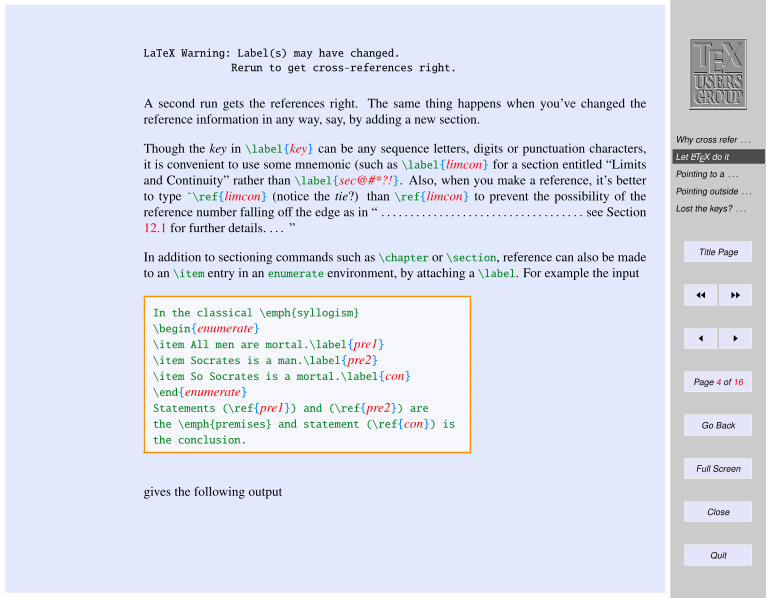
Why cross refer . . .
Let LATEX do it
Pointing to a . . .
Pointing outside . . .
Lost the keys? . . .
Title Page
JJ II
J I
Page 4 of 16
Go Back
Full Screen
Close
Quit
LaTeX Warning: Label(s) may have changed.
Rerun to get cross-references right.
A second run gets the references right. The same thing happens when you’ve changed thereference information in any way, say, by adding a new section.
Though the key in \labelkey can be any sequence letters, digits or punctuation characters,it is convenient to use some mnemonic (such as \labellimcon for a section entitled “Limitsand Continuity” rather than \labelsec@#*?!. Also, when you make a reference, it’s betterto type ˜\reflimcon (notice the tie?) than \reflimcon to prevent the possibility of thereference number falling off the edge as in “ . . . . . . . . . . . . . . . . . . . . . . . . . . . . . . . . . . . see Section12.1 for further details. . . . ”
In addition to sectioning commands such as \chapter or \section, reference can also be madeto an \item entry in an enumerate environment, by attaching a \label. For example the input
In the classical \emphsyllogism
\beginenumerate\item All men are mortal.\labelpre1\item Socrates is a man.\labelpre2\item So Socrates is a mortal.\labelcon\endenumerateStatements (\refpre1) and (\refpre2) are
the \emphpremises and statement (\refcon) is
the conclusion.
gives the following output
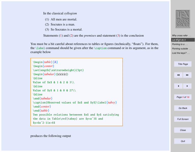
Why cross refer . . .
Let LATEX do it
Pointing to a . . .
Pointing outside . . .
Lost the keys? . . .
Title Page
JJ II
J I
Page 5 of 16
Go Back
Full Screen
Close
Quit
In the classical syllogism
(1) All men are mortal.(2) Socrates is a man.(3) So Socrates is a mortal.
Statements (1) and (2) are the premises and statement (3) is the conclusion
You must be a bit careful about references to tables or figures (technically, “floats”). For them,the \label command should be given after the \caption command or in its argument, as in theexample below
\begintable[h]\begincenter\setlength\extrarowheight5pt
\begintabular|c|c|c|c|\hline
Value of $x$ & 1 & 2 & 3\\
\hline
Value of $y$ & 1 & 8 & 27\\
\hline
\endtabular\captionObserved values of $x$ and $y$\labeltabxy\endcenter\endtableTwo possible relations betweeen $x$ and $y$ satisfying
the data in Table\reftabxy are $y=xˆ3$ and
$y=6xˆ2-11x+6$
produces the following output
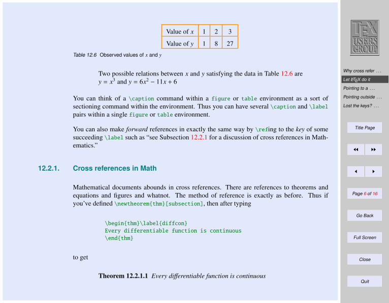
Why cross refer . . .
Let LATEX do it
Pointing to a . . .
Pointing outside . . .
Lost the keys? . . .
Title Page
JJ II
J I
Page 6 of 16
Go Back
Full Screen
Close
Quit
Value of x 1 2 3
Value of y 1 8 27
Table 12.6 Observed values of x and y
Two possible relations between x and y satisfying the data in Table 12.6 arey = x3 and y = 6x2 − 11x + 6
You can think of a \caption command within a figure or table environment as a sort ofsectioning command within the environment. Thus you can have several \caption and \label
pairs within a single figure or table environment.
You can also make forward references in exactly the same way by \refing to the key of somesucceeding \label such as “see Subsection 12.2.1 for a discussion of cross references in Math-ematics.”
12.2.1. Cross references in Math
Mathematical documents abounds in cross references. There are references to theorems andequations and figures and whatnot. The method of reference is exactly as before. Thus ifyou’ve defined \newtheoremthm[subsection], then after typing
\beginthm\labeldiffcon
Every differentiable function is continuous
\endthm
to get
Theorem 12.2.1.1 Every differentiable function is continuous
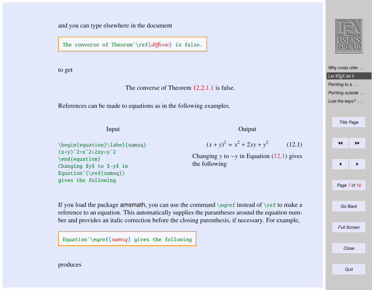
Why cross refer . . .
Let LATEX do it
Pointing to a . . .
Pointing outside . . .
Lost the keys? . . .
Title Page
JJ II
J I
Page 7 of 16
Go Back
Full Screen
Close
Quit
and you can type elsewhere in the document
The converse of Theorem˜\refdiffcon is false.
to get
The converse of Theorem 12.2.1.1 is false.
References can be made to equations as in the following examples.
Input
\beginequation\labelsumsq
(x+y)ˆ2=xˆ2+2xy+yˆ2
\endequation
Changing $y$ to $-y$ in
Equation˜(\refsumsq)
gives the following
Output
(x + y)2 = x2 + 2xy + y2 (12.1)
Changing y to −y in Equation (12.1) givesthe following
If you load the package amsmath, you can use the command \eqref instead of \ref to make areference to an equation. This automatically supplies the parantheses around the equation num-ber and provides an italic correction before the closing parenthesis, if necessary. For example,
Equation˜\eqrefsumsq gives the following
produces
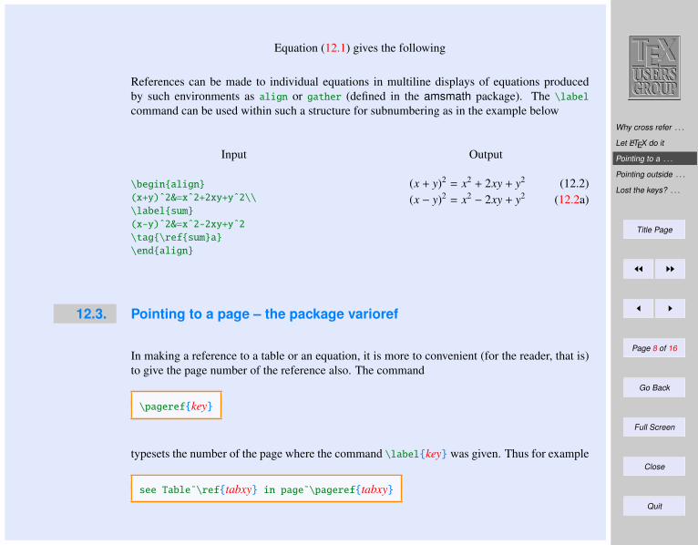
Why cross refer . . .
Let LATEX do it
Pointing to a . . .
Pointing outside . . .
Lost the keys? . . .
Title Page
JJ II
J I
Page 8 of 16
Go Back
Full Screen
Close
Quit
Equation (12.1) gives the following
References can be made to individual equations in multiline displays of equations producedby such environments as align or gather (defined in the amsmath package). The \label
command can be used within such a structure for subnumbering as in the example below
Input
\beginalign
(x+y)ˆ2&=xˆ2+2xy+yˆ2\\
\labelsum
(x-y)ˆ2&=xˆ2-2xy+yˆ2
\tag\refsuma
\endalign
Output
(x + y)2 = x2 + 2xy + y2 (12.2)(x − y)2 = x2 − 2xy + y2 (12.2a)
12.3. Pointing to a page – the package varioref
In making a reference to a table or an equation, it is more to convenient (for the reader, that is)to give the page number of the reference also. The command
\pagerefkey
typesets the number of the page where the command \labelkey was given. Thus for example
see Table˜\reftabxy in page˜\pagereftabxy
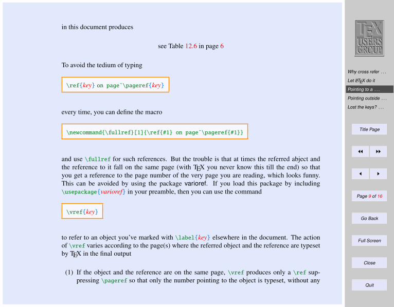
Why cross refer . . .
Let LATEX do it
Pointing to a . . .
Pointing outside . . .
Lost the keys? . . .
Title Page
JJ II
J I
Page 9 of 16
Go Back
Full Screen
Close
Quit
in this document produces
see Table 12.6 in page 6
To avoid the tedium of typing
\refkey on page˜\pagerefkey
every time, you can define the macro
\newcommand\fullref[1]\ref#1 on page˜\pageref#1
and use \fullref for such references. But the trouble is that at times the referred abject andthe reference to it fall on the same page (with TEX you never know this till the end) so thatyou get a reference to the page number of the very page you are reading, which looks funny.This can be avoided by using the package varioref. If you load this package by including\usepackagevarioref in your preamble, then you can use the command
\vrefkey
to refer to an object you’ve marked with \labelkey elsewhere in the document. The actionof \vref varies according to the page(s) where the referred object and the reference are typesetby TEX in the final output
(1) If the object and the reference are on the same page, \vref produces only a \ref sup-pressing \pageref so that only the number pointing to the object is typeset, without any
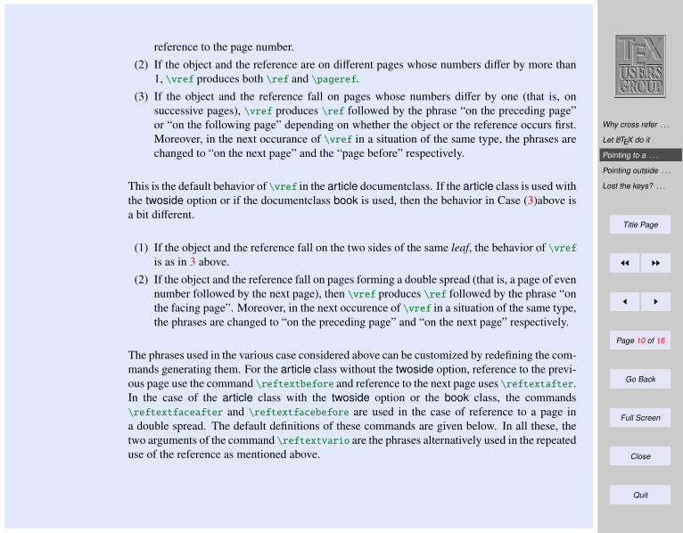
Why cross refer . . .
Let LATEX do it
Pointing to a . . .
Pointing outside . . .
Lost the keys? . . .
Title Page
JJ II
J I
Page 10 of 16
Go Back
Full Screen
Close
Quit
reference to the page number.(2) If the object and the reference are on different pages whose numbers differ by more than
1, \vref produces both \ref and \pageref.(3) If the object and the reference fall on pages whose numbers differ by one (that is, on
successive pages), \vref produces \ref followed by the phrase “on the preceding page”or “on the following page” depending on whether the object or the reference occurs first.Moreover, in the next occurance of \vref in a situation of the same type, the phrases arechanged to “on the next page” and the “page before” respectively.
This is the default behavior of \vref in the article documentclass. If the article class is used withthe twoside option or if the documentclass book is used, then the behavior in Case (3)above isa bit different.
(1) If the object and the reference fall on the two sides of the same leaf, the behavior of \vrefis as in 3 above.
(2) If the object and the reference fall on pages forming a double spread (that is, a page of evennumber followed by the next page), then \vref produces \ref followed by the phrase “onthe facing page”. Moreover, in the next occurence of \vref in a situation of the same type,the phrases are changed to “on the preceding page” and “on the next page” respectively.
The phrases used in the various case considered above can be customized by redefining the com-mands generating them. For the article class without the twoside option, reference to the previ-ous page use the command \reftextbefore and reference to the next page uses \reftextafter.In the case of the article class with the twoside option or the book class, the commands\reftextfaceafter and \reftextfacebefore are used in the case of reference to a page ina double spread. The default definitions of these commands are given below. In all these, thetwo arguments of the command \reftextvario are the phrases alternatively used in the repeateduse of the reference as mentioned above.
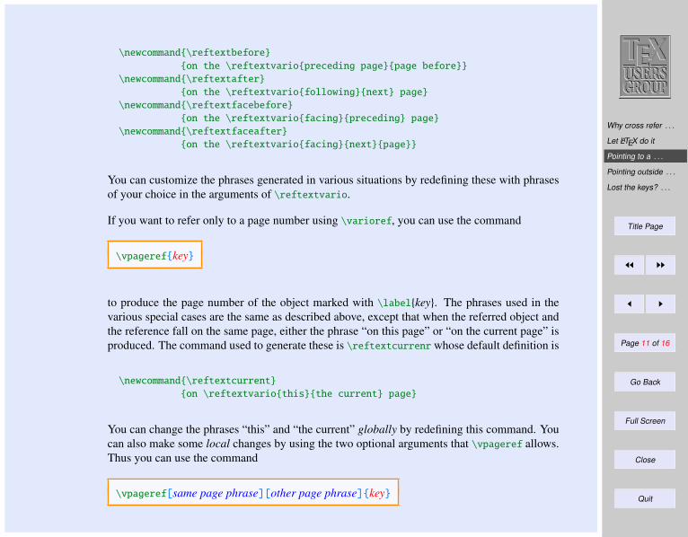
Why cross refer . . .
Let LATEX do it
Pointing to a . . .
Pointing outside . . .
Lost the keys? . . .
Title Page
JJ II
J I
Page 11 of 16
Go Back
Full Screen
Close
Quit
\newcommand\reftextbefore
on the \reftextvariopreceding pagepage before
\newcommand\reftextafter
on the \reftextvariofollowingnext page
\newcommand\reftextfacebefore
on the \reftextvariofacingpreceding page
\newcommand\reftextfaceafter
on the \reftextvariofacingnextpage
You can customize the phrases generated in various situations by redefining these with phrasesof your choice in the arguments of \reftextvario.
If you want to refer only to a page number using \varioref, you can use the command
\vpagerefkey
to produce the page number of the object marked with \labelkey. The phrases used in thevarious special cases are the same as described above, except that when the referred object andthe reference fall on the same page, either the phrase “on this page” or “on the current page” isproduced. The command used to generate these is \reftextcurrenr whose default definition is
\newcommand\reftextcurrent
on \reftextvariothisthe current page
You can change the phrases “this” and “the current” globally by redefining this command. Youcan also make some local changes by using the two optional arguments that \vpageref allows.Thus you can use the command
\vpageref[same page phrase][other page phrase]key
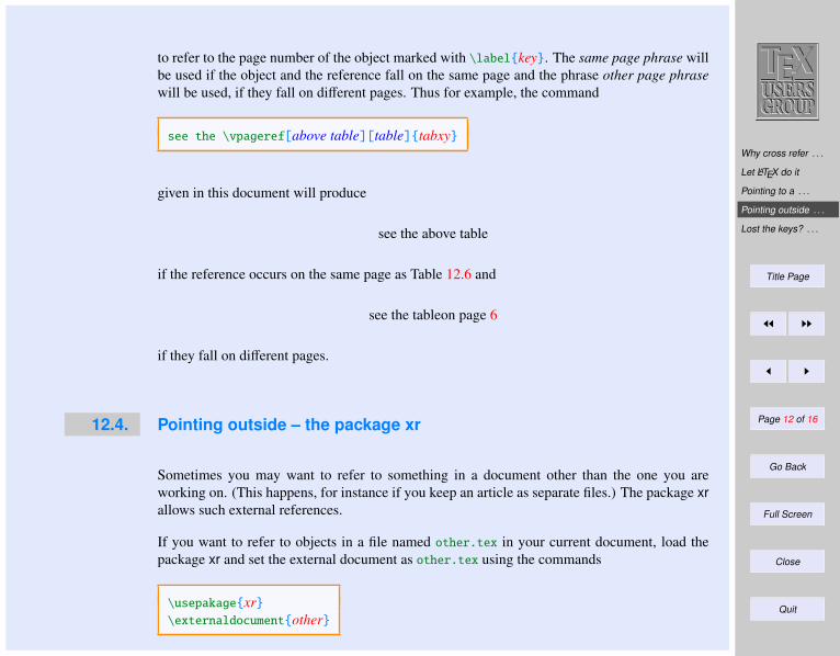
Why cross refer . . .
Let LATEX do it
Pointing to a . . .
Pointing outside . . .
Lost the keys? . . .
Title Page
JJ II
J I
Page 12 of 16
Go Back
Full Screen
Close
Quit
to refer to the page number of the object marked with \labelkey. The same page phrase willbe used if the object and the reference fall on the same page and the phrase other page phrasewill be used, if they fall on different pages. Thus for example, the command
see the \vpageref[above table][table]tabxy
given in this document will produce
see the above table
if the reference occurs on the same page as Table 12.6 and
see the tableon page 6
if they fall on different pages.
12.4. Pointing outside – the package xr
Sometimes you may want to refer to something in a document other than the one you areworking on. (This happens, for instance if you keep an article as separate files.) The package xrallows such external references.
If you want to refer to objects in a file named other.tex in your current document, load thepackage xr and set the external document as other.tex using the commands
\usepakagexr\externaldocumentother
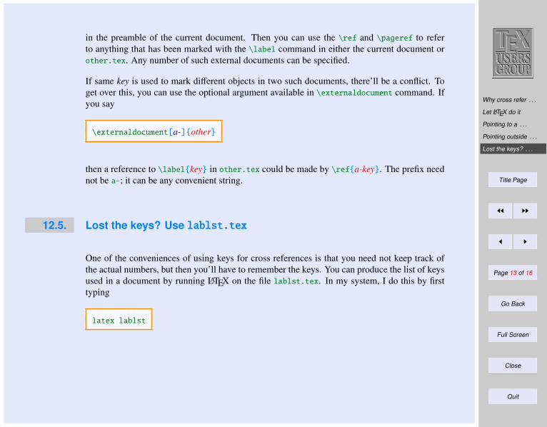
Why cross refer . . .
Let LATEX do it
Pointing to a . . .
Pointing outside . . .
Lost the keys? . . .
Title Page
JJ II
J I
Page 13 of 16
Go Back
Full Screen
Close
Quit
in the preamble of the current document. Then you can use the \ref and \pageref to referto anything that has been marked with the \label command in either the current document orother.tex. Any number of such external documents can be specified.
If same key is used to mark different objects in two such documents, there’ll be a conflict. Toget over this, you can use the optional argument available in \externaldocument command. Ifyou say
\externaldocument[a-]other
then a reference to \labelkey in other.tex could be made by \refa-key. The prefix neednot be a-; it can be any convenient string.
12.5. Lost the keys? Use lablst.tex
One of the conveniences of using keys for cross references is that you need not keep track ofthe actual numbers, but then you’ll have to remember the keys. You can produce the list of keysused in a document by running LATEX on the file lablst.tex. In my system, I do this by firsttyping
latex lablst
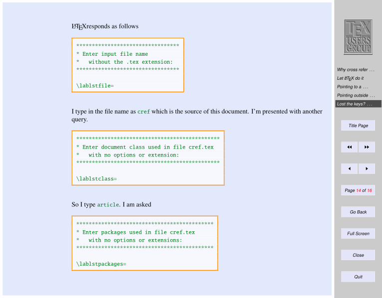
Why cross refer . . .
Let LATEX do it
Pointing to a . . .
Pointing outside . . .
Lost the keys? . . .
Title Page
JJ II
J I
Page 14 of 16
Go Back
Full Screen
Close
Quit
LATEXresponds as follows
*********************************
* Enter input file name
* without the .tex extension:
*********************************
\lablstfile=
I type in the file name as cref which is the source of this document. I’m presented with anotherquery.
**********************************************
* Enter document class used in file cref.tex
* with no options or extension:
**********************************************
\lablstclass=
So I type article. I am asked
********************************************
* Enter packages used in file cref.tex
* with no options or extensions:
********************************************
\lablstpackages=
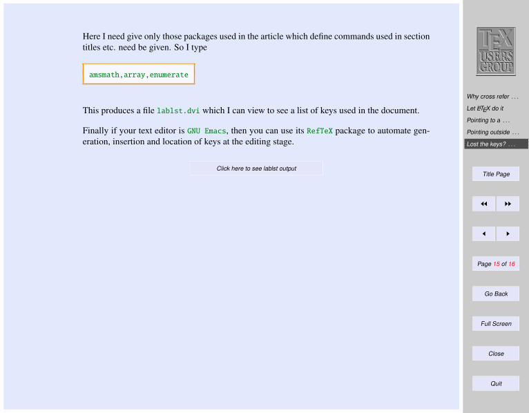
Why cross refer . . .
Let LATEX do it
Pointing to a . . .
Pointing outside . . .
Lost the keys? . . .
Title Page
JJ II
J I
Page 15 of 16
Go Back
Full Screen
Close
Quit
Here I need give only those packages used in the article which define commands used in sectiontitles etc. need be given. So I type
amsmath,array,enumerate
This produces a file lablst.dvi which I can view to see a list of keys used in the document.
Finally if your text editor is GNU Emacs, then you can use its RefTeX package to automate gen-eration, insertion and location of keys at the editing stage.
Click here to see lablst output
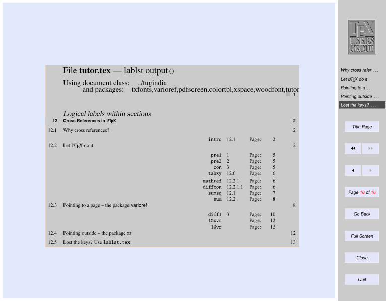
Why cross refer . . .
Let LATEX do it
Pointing to a . . .
Pointing outside . . .
Lost the keys? . . .
Title Page
JJ II
J I
Page 16 of 16
Go Back
Full Screen
Close
Quit
1
File tutor.tex — lablst output ()
Using document class: ../tugindiaand packages: txfonts,varioref,pdfscreen,colortbl,xspace,woodfont,tutorial,longtable,hhline,ifthen,layout,fancybox,boxedminipage,amscd, anysize,array
Logical labels within sections12 Cross References in LATEX 2
12.1 Why cross references? 2
intro 12.1 Page: 212.2 Let LATEX do it 2
pre1 1 Page: 5pre2 2 Page: 5con 3 Page: 5
tabxy 12.6 Page: 6mathref 12.2.1 Page: 6diffcon 12.2.1.1 Page: 6
sumsq 12.1 Page: 7sum 12.2 Page: 8
12.3 Pointing to a page – the package varioref 8
diff1 3 Page: 101@xvr Page: 121@vr Page: 12
12.4 Pointing outside – the package xr 12
12.5 Lost the keys? Use lablst.tex 13
Bibliography logical labels
Page layout in LATEX
Groups
Creating a . . .
Fun with floats
Items and lists
Some more tricks
Title Page
JJ II
J I
Page 1 of 23
Go Back
Full Screen
Close
Quit
Indian TEX Users Group: http://www.river-valley.com/tug
13On-line Tutorial on LATEX
The Tutorial TeamIndian TEX Users Group, Buildings, Cotton Hills
Trivandrum 695014, 2000
Prof. (Dr.) K. S. S. Nambooripad, Director, Center for Mathematical Sciences, Trivandrum, (Editor); Dr. E. Krishnan, Readerin Mathematics, University College, Trivandrum; Mohit Agarwal, Department of Aerospace Engineering, Indian Institute of
Science, Bangalore; T. Rishi, Focal Image (India) Pvt. Ltd., Trivandrum; L. A. Ajith, Focal Image (India) Pvt. Ltd.,Trivandrum; A. M. Shan, Focal Image (India) Pvt. Ltd., Trivandrum; C. V. Radhakrishnan, River Valley Technologies,
Software Technology Park, Trivandrum constitute the Tutorial team
This document is generated from LATEX sources compiled with pdfLATEX v. 14e in an INTEL
Pentium III 700 MHz system running Linux kernel version 2.2.14-12. The packages usedare hyperref.sty and pdfscreen.sty
c©2000, Indian TEX Users Group. This document may be distributed under the terms of the LATEXProject Public License, as described in lppl.txt in the base LATEX distribution, either version 1.0
or, at your option, any later version
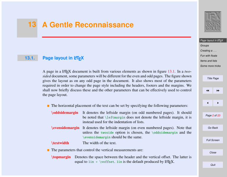
Page layout in LATEX
Groups
Creating a . . .
Fun with floats
Items and lists
Some more tricks
Title Page
JJ II
J I
Page 2 of 23
Go Back
Full Screen
Close
Quit
13 A Gentle Reconnaissance
13.1. Page layout in LATEX
A page in a LATEX document is built from various elements as shown in figure 13.1. In a two-sided document, some parameters will be different for the even and odd pages. The figure showngives the layout as on any odd page in the document. It also shows most of the parametersrequired in order to change the page style including the headers, footers and the margins. Weshall now briefly discuss these and the other parameters that can be effectively used to controlthe page layout.
The horizontal placement of the text can be set by specifying the following parameters:
\oddsidemargin It denotes the leftside margin (on odd numbered pages). It shouldbe noted that \leftmargin does not denote the leftside margin, it isinstead used for the indentation of lists.
\evensidemargin It denotes the leftside margin (on even numbered pages). Note thatunless the twoside option is chosen, the \oddsidemargin and the\evensidemargin should be the same.
\textwidth The width of the text.
The parameters that control the vertical measurements are:
\topmargin Denotes the space between the header and the vertical offset. The latter isequal to 1in + \voffset. 1in is the default produced by LATEX.
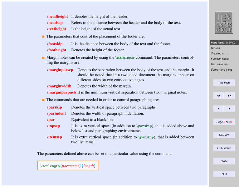
Page layout in LATEX
Groups
Creating a . . .
Fun with floats
Items and lists
Some more tricks
Title Page
JJ II
J I
Page 3 of 23
Go Back
Full Screen
Close
Quit
\headheight It denotes the height of the header.\headsep Refers to the distance between the header and the body of the text.\textheight Is the height of the actual text.
The parameters that control the placement of the footer are:
\footskip It is the distance between the body of the text and the footer.\footheight Denotes the height of the footer.
Margin notes can be created by using the \marginpar command. The parameters control-ling the margins are:
\marginparsep Denotes the separation between the body of the text and the margin. Itshould be noted that in a two-sided document the margins appear ondifferent sides on two consecutive pages.
\marginwidth Denotes the width of the margin.\marginparpush It is the minimum vertical separation between two marginal notes.
The commands that are needed in order to control paragraphing are:
\parskip Denotes the vertical space between two paragraphs.\parindent Denotes the width of paragraph indentation.\par Equivalent to a blank line.\topsep It is extra vertical space (in addition to \parskip), that is added above and
below list and paragraphing environments.\itemsep It is extra vertical space (in addition to \parskip), that is added between
two list items.
The parameters defined above can be set to a particular value using the command
\setlengthparameterlength
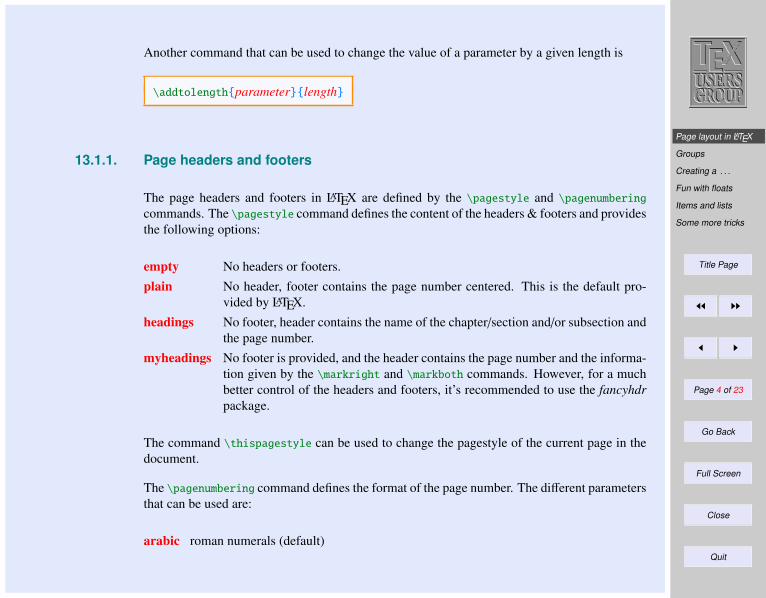
Page layout in LATEX
Groups
Creating a . . .
Fun with floats
Items and lists
Some more tricks
Title Page
JJ II
J I
Page 4 of 23
Go Back
Full Screen
Close
Quit
Another command that can be used to change the value of a parameter by a given length is
\addtolengthparameterlength
13.1.1. Page headers and footers
The page headers and footers in LATEX are defined by the \pagestyle and \pagenumbering
commands. The \pagestyle command defines the content of the headers & footers and providesthe following options:
empty No headers or footers.plain No header, footer contains the page number centered. This is the default pro-
vided by LATEX.headings No footer, header contains the name of the chapter/section and/or subsection and
the page number.myheadings No footer is provided, and the header contains the page number and the informa-
tion given by the \markright and \markboth commands. However, for a muchbetter control of the headers and footers, it’s recommended to use the fancyhdrpackage.
The command \thispagestyle can be used to change the pagestyle of the current page in thedocument.
The \pagenumbering command defines the format of the page number. The different parametersthat can be used are:
arabic roman numerals (default)
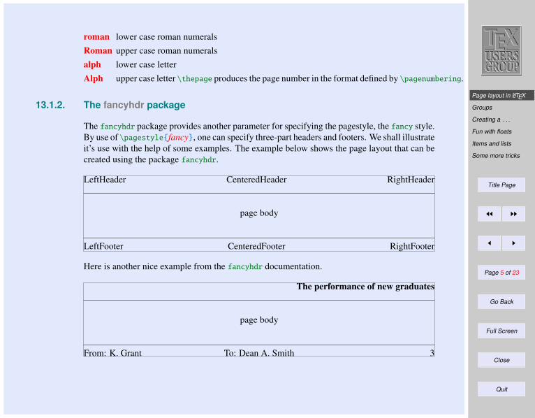
Page layout in LATEX
Groups
Creating a . . .
Fun with floats
Items and lists
Some more tricks
Title Page
JJ II
J I
Page 5 of 23
Go Back
Full Screen
Close
Quit
roman lower case roman numeralsRoman upper case roman numeralsalph lower case letterAlph upper case letter \thepage produces the page number in the format defined by \pagenumbering.
13.1.2. The fancyhdr package
The fancyhdr package provides another parameter for specifying the pagestyle, the fancy style.By use of \pagestylefancy, one can specify three-part headers and footers. We shall illustrateit’s use with the help of some examples. The example below shows the page layout that can becreated using the package fancyhdr.
LeftHeader CenteredHeader RightHeader
page body
LeftFooter CenteredFooter RightFooter
Here is another nice example from the fancyhdr documentation.
The performance of new graduates
page body
From: K. Grant To: Dean A. Smith 3
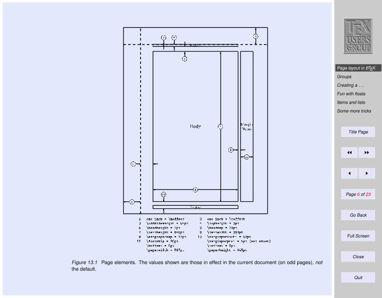
Page layout in LATEX
Groups
Creating a . . .
Fun with floats
Items and lists
Some more tricks
Title Page
JJ II
J I
Page 6 of 23
Go Back
Full Screen
Close
Quit
!"# $
!&%
'
(
!*)# $
#$!+! )-,# $
#$!.
(
'! ))
!/
'
(
('!0
('!1
('
!2
3 4&57698:5<;=?>A@&=4*BBC*6D E 4&57698:5<;=?>F@*G74*BBC*6DH @4*IIC78IJ6KLMN8:5PORQSTJD S @*D74&T&KLMN8:5UORV*TJDQ @&=76LI=76<8N=JDUORW*TJD X @&=76LIC*6*TAO?EH*TJDW @*DJ6YD=76<8N=JDUORXSJV*TJD Z @*DJ6YD[8ID=UORHXE*TJD\ @:KLMN8:5T7LMC*6*T9O93E*TJD 3V @:KLMN8:5T7LM[8ID=9O?QE*TJD33 @*B744*DC]8:TAOFHV*TJD @:KLMN8:5T7LMT^<C=9O?Q*TJD`_-54*DAC=4&[5a
@&=4*BBC*6DFOFV*TJD @*G74*BBC*6DFO?V*TJD@&T7L*T76M[8ID=9ORQ\W*TJD @&T7L*T76M=76<8N=JDAO?ZSJQ*TJD
Figure 13.1 Page elements. The values shown are those in effect in the current document (on odd pages), notthe default.
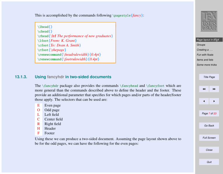
Page layout in LATEX
Groups
Creating a . . .
Fun with floats
Items and lists
Some more tricks
Title Page
JJ II
J I
Page 7 of 23
Go Back
Full Screen
Close
Quit
This is accomplished by the commands following \pagestylefancy:
\lhead
\chead
\rhead\bf The performance of new graduates\lfootFrom: K. Grant\cfootTo: Dean A. Smith\rfoot\thepage\renewcommand\headrulewidth0.4pt\renewcommand\footrulewidth0.4pt
13.1.3. Using fancyhdr in two-sided documents
The \fancyhdr package also provides the commands \fancyhead and \fancyfoot which aremore general than the commands described above to define the header and the footer. Theseprovide an additional parameter that specifies for which pages and/or parts of the header/footerthose apply. The selectors that can be used are:
E Even pageO Odd pageL Left fieldC Center fieldR Right fieldH HeaderF Footer
Using these we can produce a two-sided document. Assuming the page layout shown above tobe for the odd pages, we can have the following for the even pages:

Page layout in LATEX
Groups
Creating a . . .
Fun with floats
Items and lists
Some more tricks
Title Page
JJ II
J I
Page 8 of 23
Go Back
Full Screen
Close
Quit
The performance of new graduates
page body
4 From: K. Grant To: Dean A. Smith
This can be produced by using the commands:
\fancyhead % clear all fields\fancyhead[RO,LE]\bf The performance of new graduates\fancyfoot[LE,RO]\thepage\fancyfoot[LO,CE]From: K. Grant\fancyfoot[CO,RE]To: Dean A. Smith\renewcommand\headrulewidth0.4pt\renewcommand\footrulewidth0.4pt
The default layout in fancyhdr is produced by the following commands:
\fancyhead[LE,RO]\slshape\rightmark\fancyhead[LO,RE]\slshape\leftmark\fancyfoot[C]\thepage
The default values for \headrulewidth and \footrulewidth are 0.4pt and 0pt respectively.
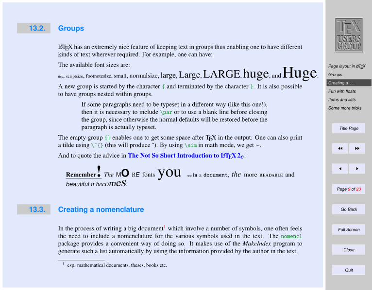
Page layout in LATEX
Groups
Creating a . . .
Fun with floats
Items and lists
Some more tricks
Title Page
JJ II
J I
Page 9 of 23
Go Back
Full Screen
Close
Quit
13.2. Groups
LATEX has an extremely nice feature of keeping text in groups thus enabling one to have differentkinds of text wherever required. For example, one can have:
The available font sizes are:
tiny, scriptsize, footnotesize, small, normalsize, large, Large, LARGE,huge, andHuge.
A new group is started by the character and terminated by the character . It is also possibleto have groups nested within groups.
If some paragraphs need to be typeset in a different way (like this one!),then it is necessary to include \par or to use a blank line before closingthe group, since otherwise the normal defaults will be restored before theparagraph is actually typeset.
The empty group enables one to get some space after TEX in the output. One can also printa tilde using \˜ (this will produce ˜). By using \sim in math mode, we get ∼.
And to quote the advice in The Not So Short Introduction to LATEX 2ε:
Remember! The MO RE fonts you use in a document, the more andbeautiful it becomes.
13.3. Creating a nomenclature
In the process of writing a big document1 which involve a number of symbols, one often feelsthe need to include a nomenclature for the various symbols used in the text. The nomencl
package provides a convenient way of doing so. It makes use of the MakeIndex program togenerate such a list automatically by using the information provided by the author in the text.
1 esp. mathematical documents, theses, books etc.
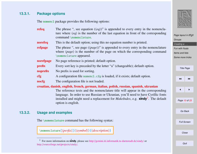
Page layout in LATEX
Groups
Creating a . . .
Fun with floats
Items and lists
Some more tricks
Title Page
JJ II
J I
Page 10 of 23
Go Back
Full Screen
Close
Quit
13.3.1. Package options
The nomencl package provides the following options:
refeq The phrase “, see equation (〈eq〉)” is appended to every entry in the nomencla-ture where 〈eq〉 is the number of the last equation in front of the correspondingcommand \nomenclature.
norefeq This is the default option; using this no equation number is printed.refpage The phrase “, see page (〈page〉)” is appended to every entry in the nomenclature
where 〈page〉 is the number of the page on which the corresponding command\nomenclature appeared.
norefpage No page reference is printed; default option.prefix Every sort key is preceded by the letter “a” (changeable); default option.noprefix No prefix is used for sorting.cfg A configuration file nomencl.cfg is loaded, if it exists; default option.nocfg The configuration file is not loaded.croatian, danish, english, french, german, italian, polish, russian, spanish, ukranian
The reference texts and the nomenclature title will appear in the correspondinglanguage. In order to use Russian or Ukranian, you’ll need to have Cyrillic fontsinstalled and might need a replacement for MakeIndex, e.g. x
ındy2. The default
option is english.
13.3.2. Usage and examples
The \nomenclature command has the following syntax:
\nomenclature[〈perfix〉]〈symbol〉〈description〉
2 For more information on xındy, please see http://gemini.iti.informatik.tu-darmstadt.de/xindy/ or
http://sourceforge.net/projects/xindy/.
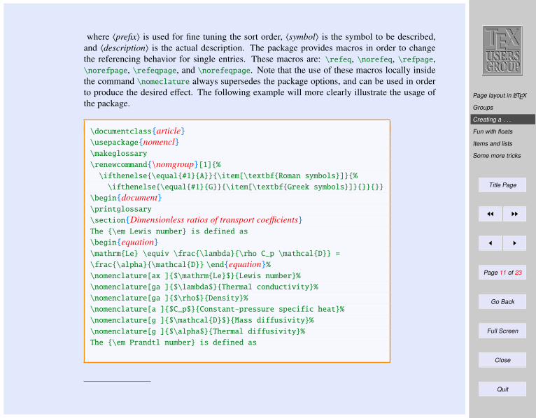
Page layout in LATEX
Groups
Creating a . . .
Fun with floats
Items and lists
Some more tricks
Title Page
JJ II
J I
Page 11 of 23
Go Back
Full Screen
Close
Quit
where 〈prefix〉 is used for fine tuning the sort order, 〈symbol〉 is the symbol to be described,and 〈description〉 is the actual description. The package provides macros in order to changethe referencing behavior for single entries. These macros are: \refeq, \norefeq, \refpage,\norefpage, \refeqpage, and \norefeqpage. Note that the use of these macros locally insidethe command \nomeclature always supersedes the package options, and can be used in orderto produce the desired effect. The following example will more clearly illustrate the usage ofthe package.
\documentclassarticle\usepackagenomencl\makeglossary
\renewcommand\nomgroup[1]%\ifthenelse\equal#1A\item[\textbfRoman symbols]%
\ifthenelse\equal#1G\item[\textbfGreek symbols]
\begindocument\printglossary
\sectionDimensionless ratios of transport coefficientsThe \em Lewis number is defined as
\beginequation\mathrmLe \equiv \frac\lambda\rho C_p \mathcalD =
\frac\alpha\mathcalD \endequation%\nomenclature[ax ]$\mathrmLe$Lewis number%
\nomenclature[ga ]$\lambda$Thermal conductivity%
\nomenclature[ga ]$\rho$Density%
\nomenclature[a ]$C_p$Constant-pressure specific heat%
\nomenclature[g ]$\mathcalD$Mass diffusivity%
\nomenclature[g ]$\alpha$Thermal diffusivity%
The \em Prandtl number is defined as
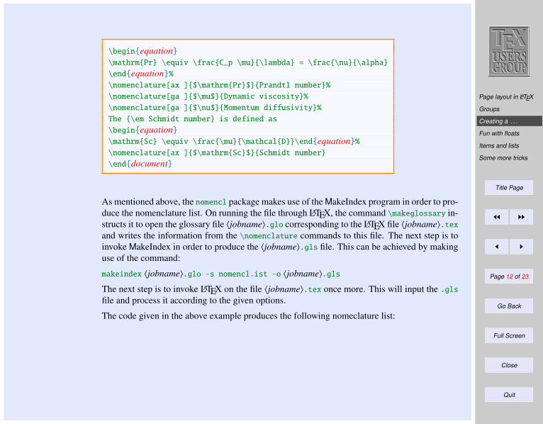
Page layout in LATEX
Groups
Creating a . . .
Fun with floats
Items and lists
Some more tricks
Title Page
JJ II
J I
Page 12 of 23
Go Back
Full Screen
Close
Quit
\beginequation\mathrmPr \equiv \fracC_p \mu\lambda = \frac\nu\alpha
\endequation%\nomenclature[ax ]$\mathrmPr$Prandtl number%
\nomenclature[ga ]$\mu$Dynamic viscosity%
\nomenclature[ga ]$\nu$Momentum diffusivity%
The \em Schmidt number is defined as
\beginequation\mathrmSc \equiv \frac\mu\mathcalD\endequation%\nomenclature[ax ]$\mathrmSc$Schmidt number
\enddocument
As mentioned above, the nomencl package makes use of the MakeIndex program in order to pro-duce the nomenclature list. On running the file through LATEX, the command \makeglossary in-structs it to open the glossary file 〈jobname〉.glo corresponding to the LATEX file 〈jobname〉.texand writes the information from the \nomenclature commands to this file. The next step is toinvoke MakeIndex in order to produce the 〈jobname〉.gls file. This can be achieved by makinguse of the command:
makeindex 〈jobname〉.glo -s nomencl.ist -o 〈jobname〉.gls
The next step is to invoke LATEX on the file 〈jobname〉.tex once more. This will input the .gls
file and process it according to the given options.
The code given in the above example produces the following nomeclature list:
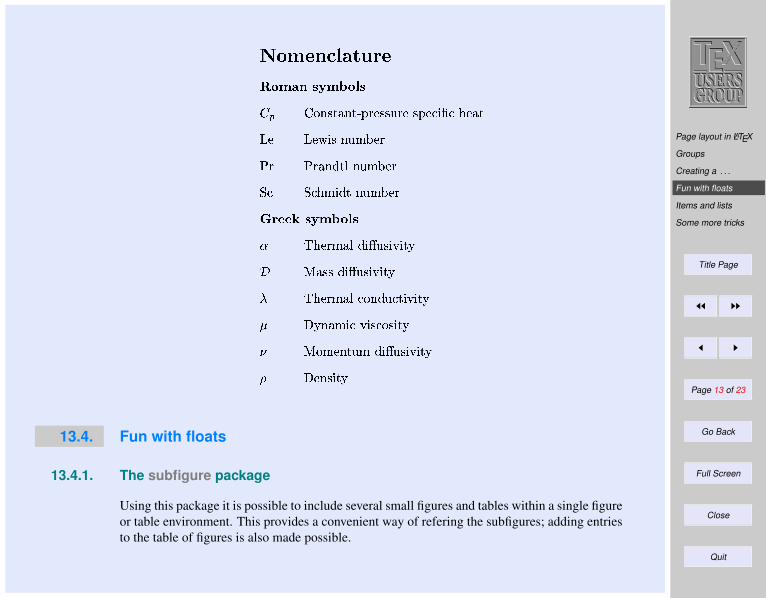
Page layout in LATEX
Groups
Creating a . . .
Fun with floats
Items and lists
Some more tricks
Title Page
JJ II
J I
Page 13 of 23
Go Back
Full Screen
Close
Quit
!#"$%&
')( *,+.-0/21435-6187:9;4< /4/8=;8<>/89?<A@BDC?@E< 351
F < F <HGIBJ/I-K=LNM<H;
O ; O ;43P-0QK14RS-6=0LNM<H;
TU@ T@VELWBXQK1Y-6=0LNM<H;
Z\[^]K]._ H!`"$%&
a b E0<H;4LW3PR!QUBDc=0/8BXd6BD1fe
g h 3P/4/IQUBicj=0/8BDdKBD1fe
k b E0<H;4LW3PR!@+.-0QU=0@18BXd6BD1fe
l m eK-035LWBJ@>dKBX/4@+6/2BD1fe
n h +PLW<H-618=0LoQUBDc=?/2BXdKBi1fe
p m <H-?/2BD1fe
13.4. Fun with floats
13.4.1. The subfigure package
Using this package it is possible to include several small figures and tables within a single figureor table environment. This provides a convenient way of refering the subfigures; adding entriesto the table of figures is also made possible.
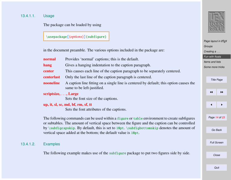
Page layout in LATEX
Groups
Creating a . . .
Fun with floats
Items and lists
Some more tricks
Title Page
JJ II
J I
Page 14 of 23
Go Back
Full Screen
Close
Quit
13.4.1.1. Usage
The package can be loaded by using
\usepackage[〈options〉]subfigure
in the document preamble. The various options included in the package are:
normal Provides ‘normal’ captions; this is the default.hang Gives a hanging indentation to the caption paragraph.center This causes each line of the caption paragraph to be separately centered.centerlast Only the last line of the caption paragraph is centered.nooneline A caption line fitting on a single line is centered by default; this option causes the
same to be left-justified.scriptsize, . . . , Large
Sets the font size of the captions.up, it, sl, sc, md, bf, rm, sf, tt
Sets the font attributes of the captions.
The following commands can be used within a figure or table environment to create subfiguresor subtables. The amount of vertical space between the figure and the caption can be controlledby \subfigcapskip. By default, this is set to 10pt. \subfigbottomskip denotes the amount ofvertical space added at the bottom; the default value is 10pt.
13.4.1.2. Examples
The following example makes use of the subfigure package to put two figures side by side.
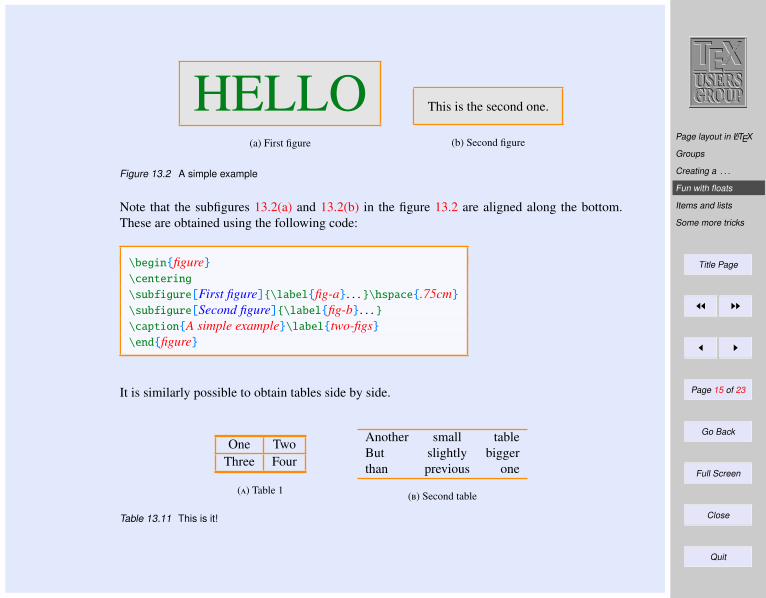
Page layout in LATEX
Groups
Creating a . . .
Fun with floats
Items and lists
Some more tricks
Title Page
JJ II
J I
Page 15 of 23
Go Back
Full Screen
Close
Quit
HELLO(a) First figure
This is the second one.
(b) Second figure
Figure 13.2 A simple example
Note that the subfigures 13.2(a) and 13.2(b) in the figure 13.2 are aligned along the bottom.These are obtained using the following code:
\beginfigure\centering
\subfigure[First figure]\labelfig-a. . . \hspace.75cm
\subfigure[Second figure]\labelfig-b. . . \captionA simple example\labeltwo-figs\endfigure
It is similarly possible to obtain tables side by side.
One TwoThree Four
() Table 1
Another small tableBut slightly biggerthan previous one
() Second table
Table 13.11 This is it!
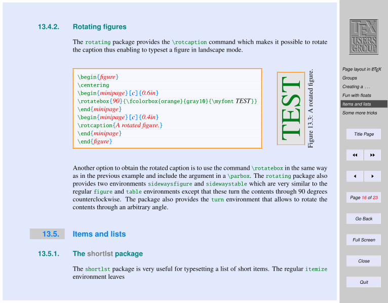
Page layout in LATEX
Groups
Creating a . . .
Fun with floats
Items and lists
Some more tricks
Title Page
JJ II
J I
Page 16 of 23
Go Back
Full Screen
Close
Quit
13.4.2. Rotating figures
The rotating package provides the \rotcaption command which makes it possible to rotatethe caption thus enabling to typeset a figure in landscape mode.
\beginfigure\centering
\beginminipage[c]0.6in\rotatebox90\fcolorboxorangegray10\myfont TEST\endminipage\beginminipage[c]0.4in\rotcaptionA rotated figure.\endminipage\endfigure T
EST
Figu
re13
.3:A
rota
ted
figur
e.
Another option to obtain the rotated caption is to use the command \rotatebox in the same wayas in the previous example and include the argument in a \parbox. The rotating package alsoprovides two environments sidewaysfigure and sidewaystable which are very similar to theregular figure and table environments except that these turn the contents through 90 degreescounterclockwise. The package also provides the turn environment that allows to rotate thecontents through an arbitrary angle.
13.5. Items and lists
13.5.1. The shortlst package
The shortlst package is very useful for typesetting a list of short items. The regular itemizeenvironment leaves
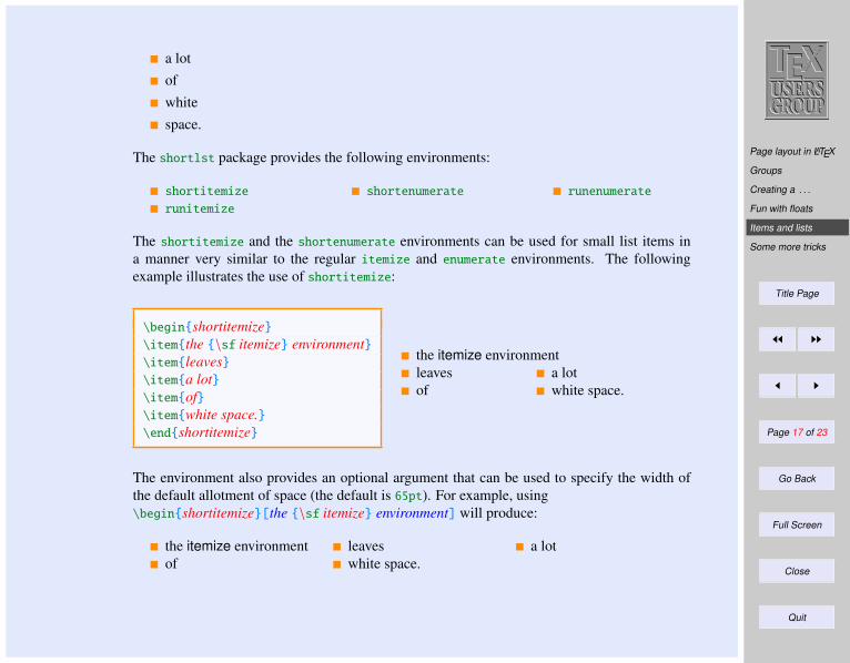
Page layout in LATEX
Groups
Creating a . . .
Fun with floats
Items and lists
Some more tricks
Title Page
JJ II
J I
Page 17 of 23
Go Back
Full Screen
Close
Quit
a lotofwhitespace.
The shortlst package provides the following environments:
shortitemize shortenumerate runenumerate
runitemize
The shortitemize and the shortenumerate environments can be used for small list items ina manner very similar to the regular itemize and enumerate environments. The followingexample illustrates the use of shortitemize:
\beginshortitemize\itemthe \sf itemize environment\itemleaves\itema lot\itemof\itemwhite space.\endshortitemize
the itemize environmentleaves a lotof white space.
The environment also provides an optional argument that can be used to specify the width ofthe default allotment of space (the default is 65pt). For example, using\beginshortitemize[the \sf itemize environment] will produce:
the itemize environment leaves a lotof white space.
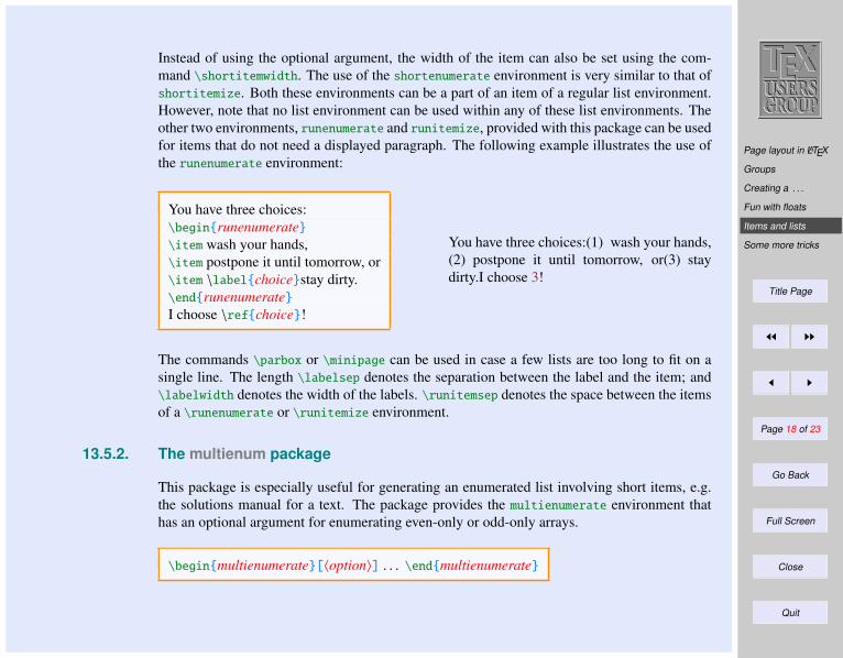
Page layout in LATEX
Groups
Creating a . . .
Fun with floats
Items and lists
Some more tricks
Title Page
JJ II
J I
Page 18 of 23
Go Back
Full Screen
Close
Quit
Instead of using the optional argument, the width of the item can also be set using the com-mand \shortitemwidth. The use of the shortenumerate environment is very similar to that ofshortitemize. Both these environments can be a part of an item of a regular list environment.However, note that no list environment can be used within any of these list environments. Theother two environments, runenumerate and runitemize, provided with this package can be usedfor items that do not need a displayed paragraph. The following example illustrates the use ofthe runenumerate environment:
You have three choices:\beginrunenumerate\item wash your hands,\item postpone it until tomorrow, or\item \labelchoicestay dirty.\endrunenumerateI choose \refchoice!
You have three choices:(1) wash your hands,(2) postpone it until tomorrow, or(3) staydirty.I choose 3!
The commands \parbox or \minipage can be used in case a few lists are too long to fit on asingle line. The length \labelsep denotes the separation between the label and the item; and\labelwidth denotes the width of the labels. \runitemsep denotes the space between the itemsof a \runenumerate or \runitemize environment.
13.5.2. The multienum package
This package is especially useful for generating an enumerated list involving short items, e.g.the solutions manual for a text. The package provides the multienumerate environment thathas an optional argument for enumerating even-only or odd-only arrays.
\beginmultienumerate[〈option〉] . . . \endmultienumerate
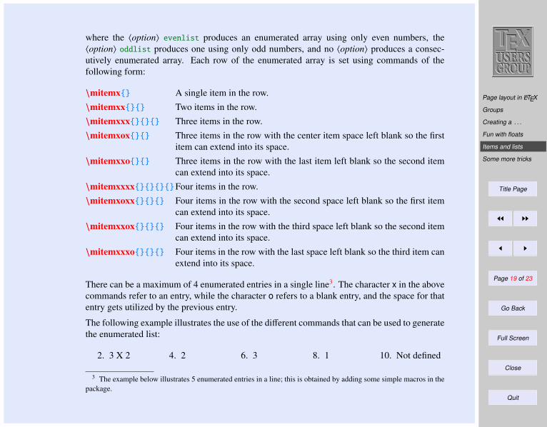
Page layout in LATEX
Groups
Creating a . . .
Fun with floats
Items and lists
Some more tricks
Title Page
JJ II
J I
Page 19 of 23
Go Back
Full Screen
Close
Quit
where the 〈option〉 evenlist produces an enumerated array using only even numbers, the〈option〉 oddlist produces one using only odd numbers, and no 〈option〉 produces a consec-utively enumerated array. Each row of the enumerated array is set using commands of thefollowing form:
\mitemx A single item in the row.\mitemxx Two items in the row.\mitemxxx Three items in the row.\mitemxox Three items in the row with the center item space left blank so the first
item can extend into its space.\mitemxxo Three items in the row with the last item left blank so the second item
can extend into its space.\mitemxxxxFour items in the row.\mitemxoxx Four items in the row with the second space left blank so the first item
can extend into its space.\mitemxxox Four items in the row with the third space left blank so the second item
can extend into its space.\mitemxxxo Four items in the row with the last space left blank so the third item can
extend into its space.
There can be a maximum of 4 enumerated entries in a single line3. The character x in the abovecommands refer to an entry, while the character o refers to a blank entry, and the space for thatentry gets utilized by the previous entry.
The following example illustrates the use of the different commands that can be used to generatethe enumerated list:
2. 3 X 2 4. 2 6. 3 8. 1 10. Not defined
3 The example below illustrates 5 enumerated entries in a line; this is obtained by adding some simple macros in thepackage.
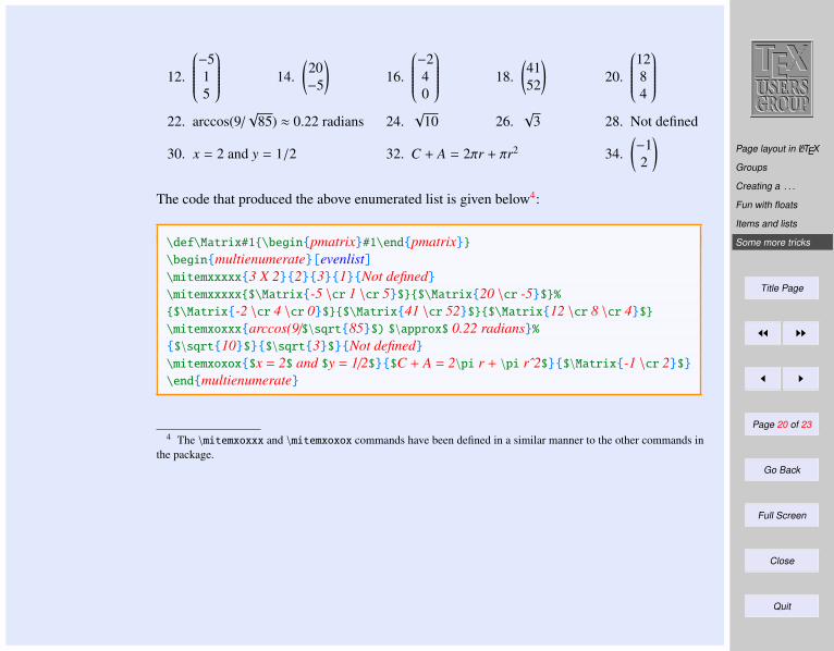
Page layout in LATEX
Groups
Creating a . . .
Fun with floats
Items and lists
Some more tricks
Title Page
JJ II
J I
Page 20 of 23
Go Back
Full Screen
Close
Quit
12.
−515
14.(20−5
)16.
−240
18.(4152
)20.
1284
22. arccos(9/
√85) ≈ 0.22 radians 24.
√10 26.
√3 28. Not defined
30. x = 2 and y = 1/2 32. C + A = 2πr + πr2 34.(−12
)The code that produced the above enumerated list is given below4:
\def\Matrix#1\beginpmatrix#1\endpmatrix\beginmultienumerate[evenlist]\mitemxxxxx3 X 2231Not defined\mitemxxxxx$\Matrix-5 \cr 1 \cr 5$$\Matrix20 \cr -5$%$\Matrix-2 \cr 4 \cr 0$$\Matrix41 \cr 52$$\Matrix12 \cr 8 \cr 4$\mitemxoxxxarccos(9/$\sqrt85$) $\approx$ 0.22 radians%$\sqrt10$$\sqrt3$Not defined\mitemxoxox$x = 2$ and $y = 1/2$$C + A = 2\pi r + \pi rˆ2$$\Matrix-1 \cr 2$\endmultienumerate
4 The \mitemxoxxx and \mitemxoxox commands have been defined in a similar manner to the other commands inthe package.
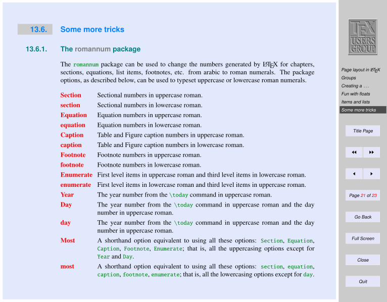
Page layout in LATEX
Groups
Creating a . . .
Fun with floats
Items and lists
Some more tricks
Title Page
JJ II
J I
Page 21 of 23
Go Back
Full Screen
Close
Quit
13.6. Some more tricks
13.6.1. The romannum package
The romannum package can be used to change the numbers generated by LATEX for chapters,sections, equations, list items, footnotes, etc. from arabic to roman numerals. The packageoptions, as described below, can be used to typeset uppercase or lowercase roman numerals.
Section Sectional numbers in uppercase roman.section Sectional numbers in lowercase roman.Equation Equation numbers in uppercase roman.equation Equation numbers in lowercase roman.Caption Table and Figure caption numbers in uppercase roman.caption Table and Figure caption numbers in lowercase roman.Footnote Footnote numbers in uppercase roman.footnote Footnote numbers in lowercase roman.Enumerate First level items in uppercase roman and third level items in lowercase roman.enumerate First level items in lowercase roman and third level items in uppercase roman.Year The year number from the \today command in uppercase roman.Day The year number from the \today command in uppercase roman and the day
number in uppercase roman.day The year number from the \today command in uppercase roman and the day
number in uppercase roman.Most A shorthand option equivalent to using all these options: Section, Equation,
Caption, Footnote, Enumerate; that is, all the uppercasing options except forYear and Day.
most A shorthand option equivalent to using all these options: section, equation,caption, footnote, enumerate; that is, all the lowercasing options except for day.
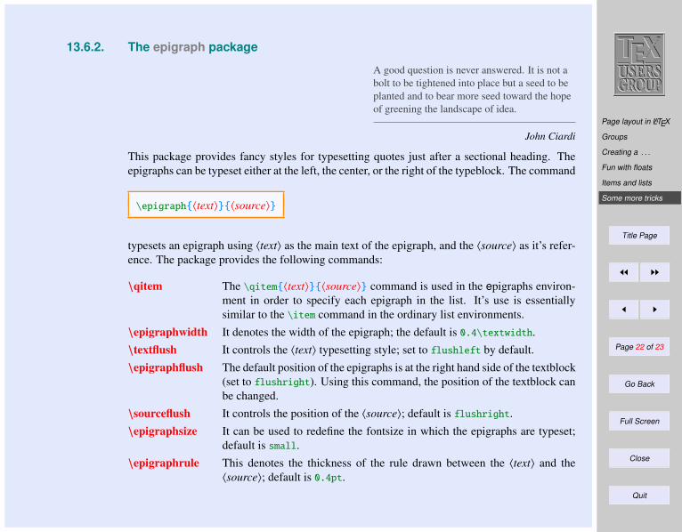
Page layout in LATEX
Groups
Creating a . . .
Fun with floats
Items and lists
Some more tricks
Title Page
JJ II
J I
Page 22 of 23
Go Back
Full Screen
Close
Quit
13.6.2. The epigraph package
A good question is never answered. It is not abolt to be tightened into place but a seed to beplanted and to bear more seed toward the hopeof greening the landscape of idea.
John Ciardi
This package provides fancy styles for typesetting quotes just after a sectional heading. Theepigraphs can be typeset either at the left, the center, or the right of the typeblock. The command
\epigraph〈text〉〈source〉
typesets an epigraph using 〈text〉 as the main text of the epigraph, and the 〈source〉 as it’s refer-ence. The package provides the following commands:
\qitem The \qitem〈text〉〈source〉 command is used in the epigraphs environ-ment in order to specify each epigraph in the list. It’s use is essentiallysimilar to the \item command in the ordinary list environments.
\epigraphwidth It denotes the width of the epigraph; the default is 0.4\textwidth.\textflush It controls the 〈text〉 typesetting style; set to flushleft by default.\epigraphflush The default position of the epigraphs is at the right hand side of the textblock
(set to flushright). Using this command, the position of the textblock canbe changed.
\sourceflush It controls the position of the 〈source〉; default is flushright.\epigraphsize It can be used to redefine the fontsize in which the epigraphs are typeset;
default is small.\epigraphrule This denotes the thickness of the rule drawn between the 〈text〉 and the
〈source〉; default is 0.4pt.
Page layout in LATEX
Groups
Creating a . . .
Fun with floats
Items and lists
Some more tricks
Title Page
JJ II
J I
Page 23 of 23
Go Back
Full Screen
Close
Quit
\beforeepigraphskip, \afterepigraphskipThese commands control the amount of vertical space instered before andafter the typeset epigraphs; default value for both the lengths is 0.5\baselineskip.
Footnotes
Marginal notes
Endnotes
Title Page
JJ II
J I
Page 1 of 12
Go Back
Full Screen
Close
Quit
Indian TEX Users Group: http://www.river-valley.com/tug
14On-line Tutorial on LATEX
The Tutorial TeamIndian TEX Users Group, Buildings, Cotton Hills
Trivandrum 695014, 2000
Prof. (Dr.) K. S. S. Nambooripad, Director, Center for Mathematical Sciences, Trivandrum, (Editor); Dr. E. Krishnan, Readerin Mathematics, University College, Trivandrum; Mohit Agarwal, Department of Aerospace Engineering, Indian Institute of
Science, Bangalore; T. Rishi, Focal Image (India) Pvt. Ltd., Trivandrum; L. A. Ajith, Focal Image (India) Pvt. Ltd.,Trivandrum; A. M. Shan, Focal Image (India) Pvt. Ltd., Trivandrum; C. V. Radhakrishnan, River Valley Technologies,
Software Technology Park, Trivandrum constitute the Tutorial team
This document is generated from LATEX sources compiled with pdfLATEX v. 14e in an INTEL
Pentium III 700 MHz system running Linux kernel version 2.2.14-12. The packages usedare hyperref.sty and pdfscreen.sty
c©2000, Indian TEX Users Group. This document may be distributed under the terms of the LATEXProject Public License, as described in lppl.txt in the base LATEX distribution, either version 1.0
or, at your option, any later version
Footnotes
Marginal notes
Endnotes
Title Page
JJ II
J I
Page 2 of 12
Go Back
Full Screen
Close
Quit
14 Footnotes, Marginpars, and Endnotes
LATEX has facilities to typeset “inserted” text, such as footnotes, marginal notes, figures andtables. This chapter looks more closely at different kinds of notes.
14.1. Footnotes
Footnotes are generated with the command
\footnotefootnote text
which comes immediately after the word requiring an explanation in a footnote. The nextfootnote text appears as a footnote in a smaller typeface at the bottom of the page. The firstline of the footnote is indented and is given the same footnote marker as that inserted in themain text. The first footnote on a page is separated from the rest of the page text by means of ashort horizontal line.
The standard footnote marker is a small, raised number1, which is sequentially numbered.
1 See how the footnote is produced: “ ... raised number \footnoteSee how the footnote is produced: ... .
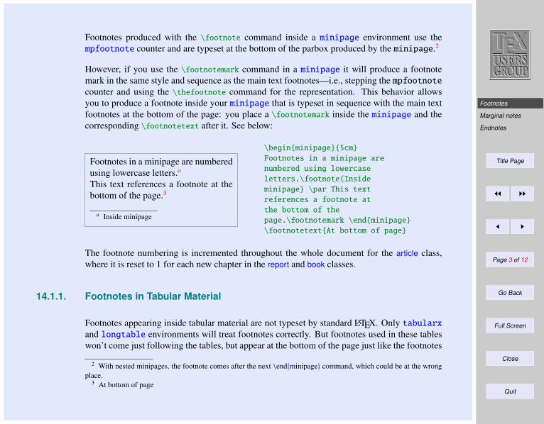
Footnotes
Marginal notes
Endnotes
Title Page
JJ II
J I
Page 3 of 12
Go Back
Full Screen
Close
Quit
Footnotes produced with the \footnote command inside a minipage environment use thempfootnote counter and are typeset at the bottom of the parbox produced by the minipage.2
However, if you use the \footnotemark command in a minipage it will produce a footnotemark in the same style and sequence as the main text footnotes—i.e., stepping the mpfootnotecounter and using the \thefootnote command for the representation. This behavior allowsyou to produce a footnote inside your minipage that is typeset in sequence with the main textfootnotes at the bottom of the page: you place a \footnotemark inside the minipage and thecorresponding \footnotetext after it. See below:
Footnotes in a minipage are numberedusing lowercase letters.a
This text references a footnote at thebottom of the page.3
a Inside minipage
\beginminipage5cm
Footnotes in a minipage are
numbered using lowercase
letters.\footnoteInside
minipage \par This text
references a footnote at
the bottom of the
page.\footnotemark \endminipage
\footnotetextAt bottom of page
The footnote numbering is incremented throughout the whole document for the article class,where it is reset to 1 for each new chapter in the report and book classes.
14.1.1. Footnotes in Tabular Material
Footnotes appearing inside tabular material are not typeset by standard LATEX. Only tabularx
and longtable environments will treat footnotes correctly. But footnotes used in these tableswon’t come just following the tables, but appear at the bottom of the page just like the footnotes
2 With nested minipages, the footnote comes after the next \endminipage command, which could be at the wrongplace.
3 At bottom of page
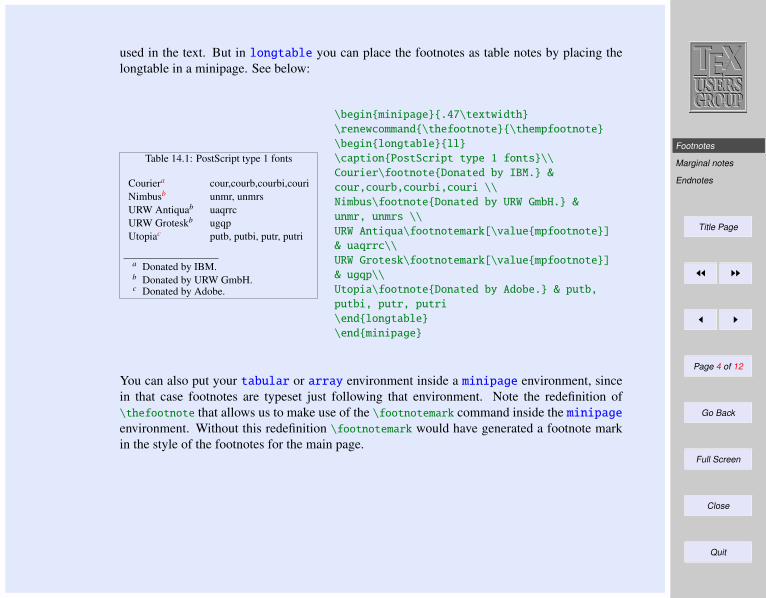
Footnotes
Marginal notes
Endnotes
Title Page
JJ II
J I
Page 4 of 12
Go Back
Full Screen
Close
Quit
used in the text. But in longtable you can place the footnotes as table notes by placing thelongtable in a minipage. See below:
Table 14.1: PostScript type 1 fonts
Couriera cour,courb,courbi,couriNimbusb unmr, unmrsURW Antiquab uaqrrcURW Groteskb ugqpUtopiac putb, putbi, putr, putri
a Donated by IBM.b Donated by URW GmbH.c Donated by Adobe.
\beginminipage.47\textwidth
\renewcommand\thefootnote\thempfootnote
\beginlongtablell
\captionPostScript type 1 fonts\\
Courier\footnoteDonated by IBM. &
cour,courb,courbi,couri \\
Nimbus\footnoteDonated by URW GmbH. &
unmr, unmrs \\
URW Antiqua\footnotemark[\valuempfootnote]
& uaqrrc\\
URW Grotesk\footnotemark[\valuempfootnote]
& ugqp\\
Utopia\footnoteDonated by Adobe. & putb,
putbi, putr, putri
\endlongtable
\endminipage
You can also put your tabular or array environment inside a minipage environment, sincein that case footnotes are typeset just following that environment. Note the redefinition of\thefootnote that allows us to make use of the \footnotemark command inside the minipageenvironment. Without this redefinition \footnotemark would have generated a footnote markin the style of the footnotes for the main page.
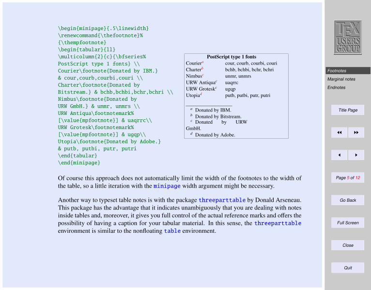
Footnotes
Marginal notes
Endnotes
Title Page
JJ II
J I
Page 5 of 12
Go Back
Full Screen
Close
Quit
\beginminipage.5\linewidth
\renewcommand\thefootnote%
\thempfootnote
\begintabularll
\multicolumn2c\bfseries%
PostScript type 1 fonts \\
Courier\footnoteDonated by IBM.
& cour,courb,courbi,couri \\
Charter\footnoteDonated by
Bitstream. & bchb,bchbi,bchr,bchri \\
Nimbus\footnoteDonated by
URW GmbH. & unmr, unmrs \\
URW Antiqua\footnotemark%
[\valuempfootnote] & uaqrrc\\
URW Grotesk\footnotemark%
[\valuempfootnote] & ugqp\\
Utopia\footnoteDonated by Adobe.
& putb, putbi, putr, putri
\endtabular
\endminipage
PostScript type 1 fontsCouriera cour, courb, courbi, couriCharterb bchb, bchbi, bchr, bchriNimbusc unmr, unmrsURW Antiquac uaqrrcURW Groteskc ugqpUtopiad putb, putbi, putr, putri
a Donated by IBM.b Donated by Bitstream.c Donated by URW
GmbH.d Donated by Adobe.
Of course this approach does not automatically limit the width of the footnotes to the width ofthe table, so a little iteration with the minipage width argument might be necessary.
Another way to typeset table notes is with the package threeparttable by Donald Arseneau.This package has the advantage that it indicates unambiguously that you are dealing with notesinside tables and, moreover, it gives you full control of the actual reference marks and offers thepossibility of having a caption for your tabular material. In this sense, the threeparttable
environment is similar to the nonfloating table environment.
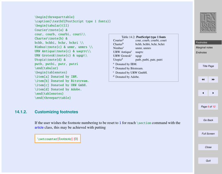
Footnotes
Marginal notes
Endnotes
Title Page
JJ II
J I
Page 6 of 12
Go Back
Full Screen
Close
Quit
\beginthreeparttable
\caption\textbfPostScript type 1 fonts
\begintabularll
Courier\tnotea &
cour, courb, courbi, couri\\
Charter\tnoteb &
bchb, bchbi, bchr, bchri \\
Nimbus\tnotec & unmr, unmrs \\
URW Antiqua\tnotec & uaqrrc\\
URW Grotesk\tnotec & ugqp\\
Utopia\tnoted &
putb, putbi, putr, putri
\endtabular
\begintablenotes
\item[a] Donated by IBM.
\item[b] Donated by Bitstream.
\item[c] Donated by URW GmbH.
\item[d] Donated by Adobe.
\endtablenotes
\endthreeparttable
Table 14.2: PostScript type 1 fontsCouriera cour, courb, courbi, couriCharterb bchb, bchbi, bchr, bchriNimbusc unmr, unmrsURW Antiquac uaqrrcURW Groteskc ugqpUtopiad putb, putbi, putr, putria Donated by IBM.b Donated by Bitstream.c Donated by URW GmbH.d Donated by Adobe.
14.1.2. Customizing footnotes
If the user wishes the footnote numbering to be reset to 1 for reach \section command with thearticle class, this may be achieved with putting
\setcounterfootnote 0
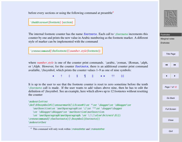
Footnotes
Marginal notes
Endnotes
Title Page
JJ II
J I
Page 7 of 12
Go Back
Full Screen
Close
Quit
before every sections or using the following command at preamble4
\@addtoresetfootnote section
The internal footnote counter has the name footnote. Each call to \footnote increments thiscounter by one and prints the new value in Arabic numbering as the footnote marker. A differentstyle of marker can be implemented with the command
\renewcommand\thefootnote\number stylefootnote
where number style is one of the counter print commands. \arabic, \roman, \Roman, \alph,or \Alph. However, for the counter footnote, there is an additional counter print commandavailable, \fnsymbol, which prints the counter values 1–9 as one of nine symbols:
? † ‡ § ¶ ‖ ? ? †† ‡‡
It is up to the user to see that the footnote counter is reset to zero sometime before the tenth\footnote call is made. If the user wants to add values above nine, then he has to edit thedefinition of \fnsymbol. See an example, here which allows up to 12 footnotes without resettingthe counter
\makeatletter
\def\@fnsymbol#1\ensuremath\ifcase#1\or *\or \dagger\or \ddagger\or
\mathsection\or \mathparagraph\or \|\or **\or \dagger\dagger
\or \ddagger\ddagger\or \mathsection\mathsection
\or \mathparagraph\mathparagraph \or \|\|\else\@ctrerr\fi
\renewcommand\thefootnote\fnsymbolfootnote
\makeatother
4 This command will only work within \makeatletter and \makeatother
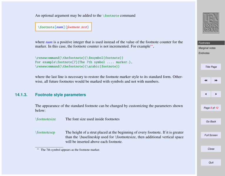
Footnotes
Marginal notes
Endnotes
Title Page
JJ II
J I
Page 8 of 12
Go Back
Full Screen
Close
Quit
An optional argument may be added to the \footnote command
\footnote[num]footnote text
where num is a positive integer that is used instead of the value of the footnote counter for themarker. In this case, the footnote counter is not incremented. For example∗∗,
\renewcommand\thefootnote\fnsymbolfootnote
For example\footnote[7]The 7th symbol .... marker.,
\renewcommand\thefootnote\arabicfootnote
where the last line is necessary to restore the footnote marker style to its standard form. Other-wise, all future footnotes would be marked with symbols and not with numbers.
14.1.3. Footnote style parameters
The appearance of the standard footnote can be changed by customizing the parameters shownbelow:
\footnotesize The font size used inside footnotes
\footnotesep The height of a strut placed at the beginning of every footnote. If it is greaterthan the \baselineskip used for \footnotesize, then additional vertical spacewill be inserted above each footnote.
∗∗ The 7th symbol appears as the footnote marker.
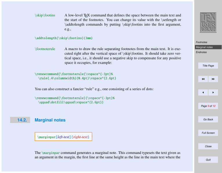
Footnotes
Marginal notes
Endnotes
Title Page
JJ II
J I
Page 9 of 12
Go Back
Full Screen
Close
Quit
\skip\footins A low-level TEX command that defines the space between the main text andthe start of the footnotes. You can change its value with the \setlength or\addtolength commands by putting \skip\footins into the first argument,e.g.,
\addtolength\skip\footins3mm
\footnoterule A macro to draw the rule separating footnotes from the main text. It is exe-cuted right after the vertical space of \skip\footins. It should take zero ver-tical space, i.e., it should use a negative skip to compensate for any positivespace it occupies, for example:
\renewcommand\footnoterule\vspace*-3pt%
\rule.4\columnwidth0.4pt\vspace*2.6pt
You can also construct a fancier “rule” e.g., one consisting of a series of dots:
\renewcommand\footnoterule\vspace*-3pt%
\qquad\dotfill\qquad\vspace*2.6pt
14.2. Marginal notes
\marginpar[left-text]right-text
The \marginpar command generates a marginal note. This command typesets the text given asan argument in the margin, the first line at the same height as the line in the main text where the
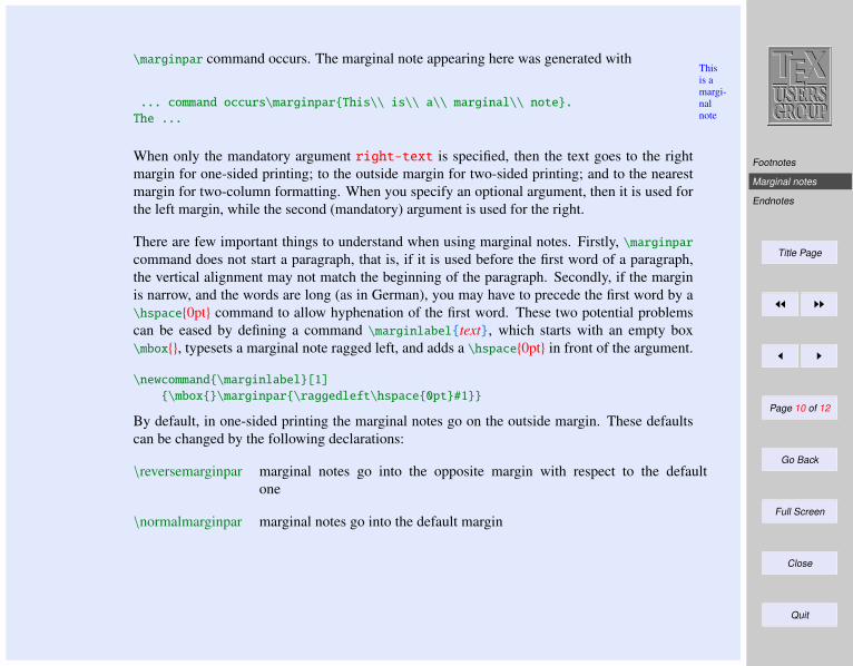
Footnotes
Marginal notes
Endnotes
Title Page
JJ II
J I
Page 10 of 12
Go Back
Full Screen
Close
Quit
\marginpar command occurs. The marginal note appearing here was generated withThisis amargi-nalnote
... command occurs\marginparThis\\ is\\ a\\ marginal\\ note.
The ...
When only the mandatory argument right-text is specified, then the text goes to the rightmargin for one-sided printing; to the outside margin for two-sided printing; and to the nearestmargin for two-column formatting. When you specify an optional argument, then it is used forthe left margin, while the second (mandatory) argument is used for the right.
There are few important things to understand when using marginal notes. Firstly, \marginparcommand does not start a paragraph, that is, if it is used before the first word of a paragraph,the vertical alignment may not match the beginning of the paragraph. Secondly, if the marginis narrow, and the words are long (as in German), you may have to precede the first word by a\hspace0pt command to allow hyphenation of the first word. These two potential problemscan be eased by defining a command \marginlabeltext, which starts with an empty box\mbox, typesets a marginal note ragged left, and adds a \hspace0pt in front of the argument.
\newcommand\marginlabel[1]
\mbox\marginpar\raggedleft\hspace0pt#1
By default, in one-sided printing the marginal notes go on the outside margin. These defaultscan be changed by the following declarations:
\reversemarginpar marginal notes go into the opposite margin with respect to the defaultone
\normalmarginpar marginal notes go into the default margin
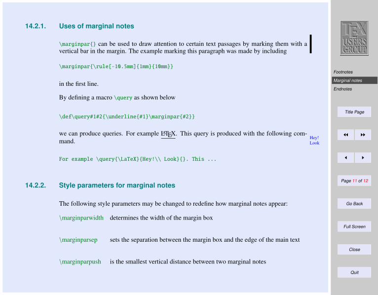
Footnotes
Marginal notes
Endnotes
Title Page
JJ II
J I
Page 11 of 12
Go Back
Full Screen
Close
Quit
14.2.1. Uses of marginal notes
\marginpar can be used to draw attention to certain text passages by marking them with avertical bar in the margin. The example marking this paragraph was made by including
\marginpar\rule[-10.5mm]1mm10mm
in the first line.
By defining a macro \query as shown below
\def\query#1#2\underline#1\marginpar#2
we can produce queries. For example LATEX. This query is produced with the following com-Hey!Lookmand.
For example \query\LaTeXHey!\\ Look. This ...
14.2.2. Style parameters for marginal notes
The following style parameters may be changed to redefine how marginal notes appear:
\marginparwidth determines the width of the margin box
\marginparsep sets the separation between the margin box and the edge of the main text
\marginparpush is the smallest vertical distance between two marginal notes
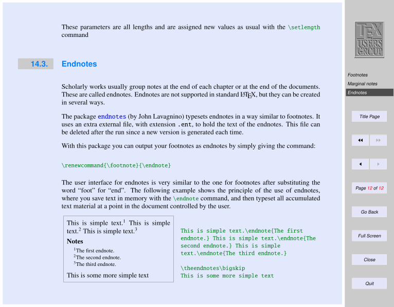
Footnotes
Marginal notes
Endnotes
Title Page
JJ II
J I
Page 12 of 12
Go Back
Full Screen
Close
Quit
These parameters are all lengths and are assigned new values as usual with the \setlength
command
14.3. Endnotes
Scholarly works usually group notes at the end of each chapter or at the end of the documents.These are called endnotes. Endnotes are not supported in standard LATEX, but they can be createdin several ways.
The package endnotes (by John Lavagnino) typesets endnotes in a way similar to footnotes. Ituses an extra external file, with extension .ent, to hold the text of the endnotes. This file canbe deleted after the run since a new version is generated each time.
With this package you can output your footnotes as endnotes by simply giving the command:
\renewcommand\footnote\endnote
The user interface for endnotes is very similar to the one for footnotes after substituting theword “foot” for “end”. The following example shows the principle of the use of endnotes,where you save text in memory with the \endnote command, and then typeset all accumulatedtext material at a point in the document controlled by the user.
This is simple text.1 This is simpletext.2 This is simple text.3
Notes1The first endnote.2The second endnote.3The third endnote.
This is some more simple text
This is simple text.\endnoteThe first
endnote. This is simple text.\endnoteThe
second endnote. This is simple
text.\endnoteThe third endnote.
\theendnotes\bigskip
This is some more simple text

The BTEX program
BTEX Style files
Creating a biblio . . .
Title Page
JJ II
J I
Page 1 of 10
Go Back
Full Screen
Close
Quit
Indian TEX Users Group: http://www.river-valley.com/tug
15On-line Tutorial on LATEX
The Tutorial TeamIndian TEX Users Group, Buildings, Cotton Hills
Trivandrum 695014, 2000
Prof. (Dr.) K. S. S. Nambooripad, Director, Center for Mathematical Sciences, Trivandrum, (Editor); Dr. E. Krishnan, Readerin Mathematics, University College, Trivandrum; Mohit Agarwal, Department of Aerospace Engineering, Indian Institute of
Science, Bangalore; T. Rishi, Focal Image (India) Pvt. Ltd., Trivandrum; L. A. Ajith, Focal Image (India) Pvt. Ltd.,Trivandrum; A. M. Shan, Focal Image (India) Pvt. Ltd., Trivandrum; C. V. Radhakrishnan, River Valley Technologies,
Software Technology Park, Trivandrum constitute the Tutorial team
This document is generated from LATEX sources compiled with pdfLATEX v. 14e in an INTEL
Pentium III 700 MHz system running Linux kernel version 2.2.14-12. The packages usedare hyperref.sty and pdfscreen.sty
c©2000, Indian TEX Users Group. This document may be distributed under the terms of the LATEXProject Public License, as described in lppl.txt in the base LATEX distribution, either version 1.0
or, at your option, any later version
The BTEX program
BTEX Style files
Creating a biblio . . .
Title Page
JJ II
J I
Page 2 of 10
Go Back
Full Screen
Close
Quit
15 Bibliographic Databases
Bibliographic Database is a database where all the useful bibliographic entries can be stored.The information about the various publications is stored in one or more files with the extension.bib. For each publication there is a key that identifies it, and which may be used in the textdocument to refer to it. And this is available for all documents with a list of reference in thefield. This database is useful for the authors/researchers who are constantly referring to thesame publications in most of their works. This database system is possible with the BTEXprogram supplied with the LATEX package.
15.1. The BTEX program
BTEX is an auxiliary program to LATEX that automatically constructs a bibliography for LATEXdocument form one or more databases. To use BTEX, you must include in your LATEX inputfile a \bibliography command whose argument specifies one or more files that contain thedatabase. For example
\bibliographydatabase1,database2
The above command specifies that the bibliographic entries are obtained from database1.biband database2.bib. To use BTEX, your LATEX input file must contain a \bibliographystyle
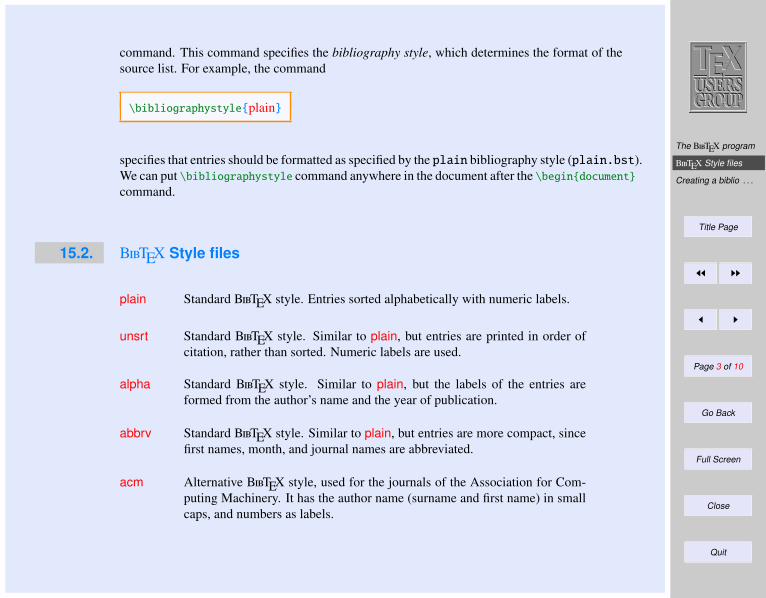
The BTEX program
BTEX Style files
Creating a biblio . . .
Title Page
JJ II
J I
Page 3 of 10
Go Back
Full Screen
Close
Quit
command. This command specifies the bibliography style, which determines the format of thesource list. For example, the command
\bibliographystyleplain
specifies that entries should be formatted as specified by the plain bibliography style (plain.bst).We can put \bibliographystyle command anywhere in the document after the \begindocumentcommand.
15.2. BTEX Style files
plain Standard BTEX style. Entries sorted alphabetically with numeric labels.
unsrt Standard BTEX style. Similar to plain, but entries are printed in order ofcitation, rather than sorted. Numeric labels are used.
alpha Standard BTEX style. Similar to plain, but the labels of the entries areformed from the author’s name and the year of publication.
abbrv Standard BTEX style. Similar to plain, but entries are more compact, sincefirst names, month, and journal names are abbreviated.
acm Alternative BTEX style, used for the journals of the Association for Com-puting Machinery. It has the author name (surname and first name) in smallcaps, and numbers as labels.
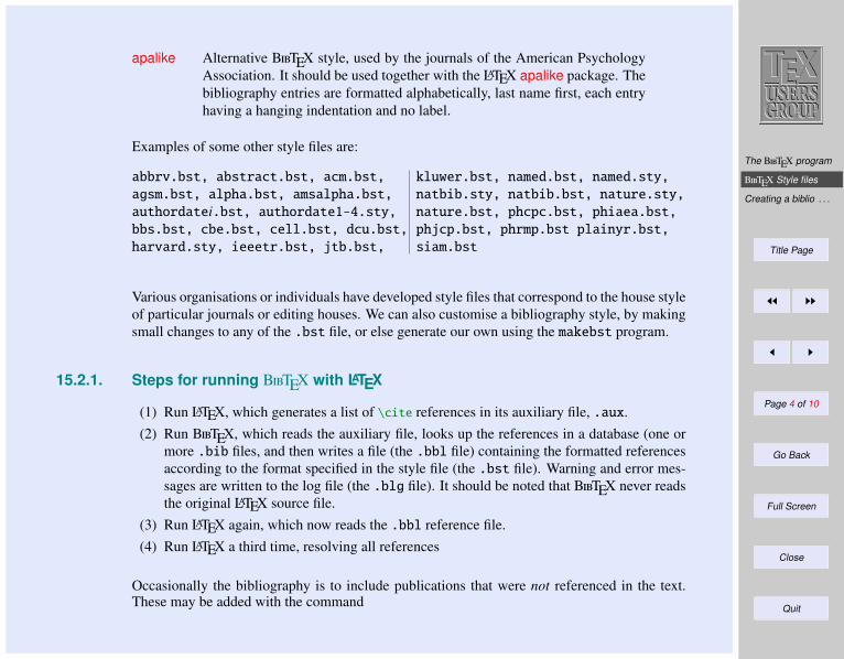
The BTEX program
BTEX Style files
Creating a biblio . . .
Title Page
JJ II
J I
Page 4 of 10
Go Back
Full Screen
Close
Quit
apalike Alternative BTEX style, used by the journals of the American PsychologyAssociation. It should be used together with the LATEX apalike package. Thebibliography entries are formatted alphabetically, last name first, each entryhaving a hanging indentation and no label.
Examples of some other style files are:
abbrv.bst, abstract.bst, acm.bst,
agsm.bst, alpha.bst, amsalpha.bst,
authordatei.bst, authordate1-4.sty,
bbs.bst, cbe.bst, cell.bst, dcu.bst,
harvard.sty, ieeetr.bst, jtb.bst,
kluwer.bst, named.bst, named.sty,
natbib.sty, natbib.bst, nature.sty,
nature.bst, phcpc.bst, phiaea.bst,
phjcp.bst, phrmp.bst plainyr.bst,
siam.bst
Various organisations or individuals have developed style files that correspond to the house styleof particular journals or editing houses. We can also customise a bibliography style, by makingsmall changes to any of the .bst file, or else generate our own using the makebst program.
15.2.1. Steps for running BTEX with LATEX
(1) Run LATEX, which generates a list of \cite references in its auxiliary file, .aux.(2) Run BTEX, which reads the auxiliary file, looks up the references in a database (one or
more .bib files, and then writes a file (the .bbl file) containing the formatted referencesaccording to the format specified in the style file (the .bst file). Warning and error mes-sages are written to the log file (the .blg file). It should be noted that BTEX never readsthe original LATEX source file.
(3) Run LATEX again, which now reads the .bbl reference file.(4) Run LATEX a third time, resolving all references
Occasionally the bibliography is to include publications that were not referenced in the text.These may be added with the command
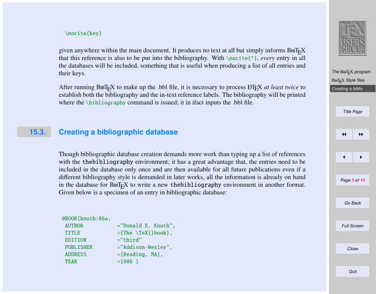
The BTEX program
BTEX Style files
Creating a biblio . . .
Title Page
JJ II
J I
Page 5 of 10
Go Back
Full Screen
Close
Quit
\nocitekey
given anywhere within the main document. It produces no text at all but simply informs BTEXthat this reference is also to be put into the bibliography. With \nocite*, every entry in allthe databases will be included, something that is useful when producing a list of all entries andtheir keys.
After running BTEX to make up the .bbl file, it is necessary to process LATEX at least twice toestablish both the bibliography and the in-text reference labels. The bibliography will be printedwhere the \bibliography command is issued; it in ifact inputs the .bbl file.
15.3. Creating a bibliographic database
Though bibliographic database creation demands more work than typing up a list of referenceswith the thebibliography environment; it has a great advantage that, the entries need to beincluded in the database only once and are then available for all future publications even if adifferent bibliography style is demanded in later works, all the information is already on handin the database for BTEX to write a new thebibliography environment in another format.Given below is a specimen of an entry in bibliographic database:
@BOOKknuth:86a,
AUTHOR ="Donald E. Knuth",
TITLE =The \TeXbook,
EDITION ="third"
PUBLISHER ="Addison-Wesley",
ADDRESS =Reading, MA,
YEAR =1986
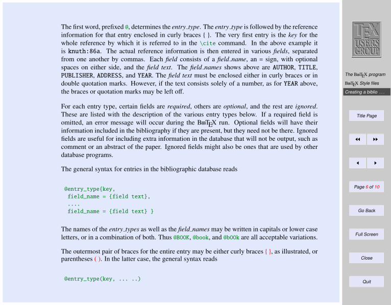
The BTEX program
BTEX Style files
Creating a biblio . . .
Title Page
JJ II
J I
Page 6 of 10
Go Back
Full Screen
Close
Quit
The first word, prefixed @, determines the entry type. The entry type is followed by the referenceinformation for that entry enclosed in curly braces . The very first entry is the key for thewhole reference by which it is referred to in the \cite command. In the above example itis knuth:86a. The actual reference information is then entered in various fields, separatedfrom one another by commas. Each field consists of a field name, an = sign, with optionalspaces on either side, and the field text. The field names shows above are AUTHOR, TITLE,PUBLISHER, ADDRESS, and YEAR. The field text must be enclosed either in curly braces or indouble quotation marks. However, if the text consists solely of a number, as for YEAR above,the braces or quotation marks may be left off.
For each entry type, certain fields are required, others are optional, and the rest are ignored.These are listed with the description of the various entry types below. If a required field isomitted, an error message will occur during the BTEX run. Optional fields will have theirinformation included in the bibliography if they are present, but they need not be there. Ignoredfields are useful for including extra information in the database that will not be output, such ascomment or an abstract of the paper. Ignored fields might also be ones that are used by otherdatabase programs.
The general syntax for entries in the bibliographic database reads
@entry_typekey,
field_name = field text,
....
field_name = field text
The names of the entry types as well as the field names may be written in capitals or lower caseletters, or in a combination of both. Thus @BOOK, @book, and @bOOk are all acceptable variations.
The outermost pair of braces for the entire entry may be either curly braces , as illustrated, orparentheses ( ). In the latter case, the general syntax reads
@entry_type(key, ... ..)
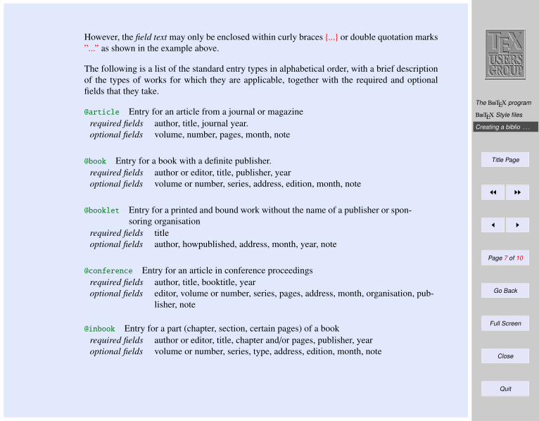
The BTEX program
BTEX Style files
Creating a biblio . . .
Title Page
JJ II
J I
Page 7 of 10
Go Back
Full Screen
Close
Quit
However, the field text may only be enclosed within curly braces ... or double quotation marks”...” as shown in the example above.
The following is a list of the standard entry types in alphabetical order, with a brief descriptionof the types of works for which they are applicable, together with the required and optionalfields that they take.
@article Entry for an article from a journal or magazinerequired fields author, title, journal year.optional fields volume, number, pages, month, note
@book Entry for a book with a definite publisher.required fields author or editor, title, publisher, yearoptional fields volume or number, series, address, edition, month, note
@booklet Entry for a printed and bound work without the name of a publisher or spon-soring organisation
required fields titleoptional fields author, howpublished, address, month, year, note
@conference Entry for an article in conference proceedingsrequired fields author, title, booktitle, yearoptional fields editor, volume or number, series, pages, address, month, organisation, pub-
lisher, note
@inbook Entry for a part (chapter, section, certain pages) of a bookrequired fields author or editor, title, chapter and/or pages, publisher, yearoptional fields volume or number, series, type, address, edition, month, note
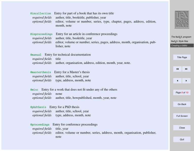
The BTEX program
BTEX Style files
Creating a biblio . . .
Title Page
JJ II
J I
Page 8 of 10
Go Back
Full Screen
Close
Quit
@incollection Entry for part of a book that has its own titlerequired fields author, title, booktitle, publisher, yearoptional fields editor, volume or number, series, type, chapter, pages, address, edition,
month, note
@inproceedings Entry for an article in conference proceedingsrequired fields author, title, booktitle, yearoptional fields editor, volume or number, series, pages, address, month, organisation, pub-
lisher, note
@manual Entry for technical documentationrequired fields titleoptional fields author, organisation, address, edition, month, year, note.
@masterthesis Entry for a Master’s thesisrequired fields author, title, school, yearoptional fields type, address, month, note
@misc Entry for a work that does not fit under any of the othersrequired fields noneoptional fields author, title, howpublished, month, year, note
@phdthesis Entry for a PhD thesisrequired fields author, title, school, yearoptional fields type, address, month, note
@proceedings Entry for conference proceedingsrequired fields title, yearoptional fields editor, volume or number, series, address, month, organisation, publisher,
note
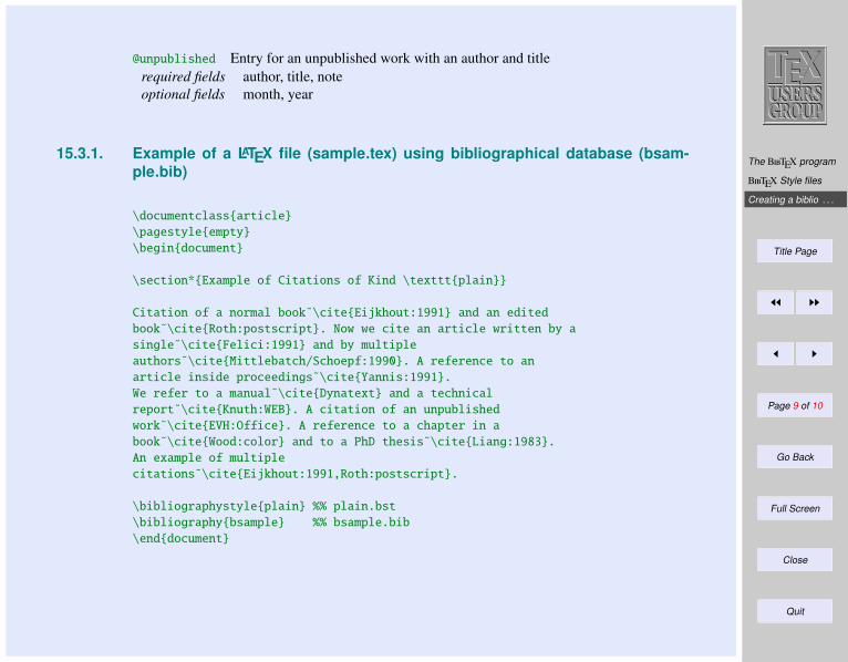
The BTEX program
BTEX Style files
Creating a biblio . . .
Title Page
JJ II
J I
Page 9 of 10
Go Back
Full Screen
Close
Quit
@unpublished Entry for an unpublished work with an author and titlerequired fields author, title, noteoptional fields month, year
15.3.1. Example of a LATEX file (sample.tex) using bibliographical database (bsam-ple.bib)
\documentclassarticle
\pagestyleempty
\begindocument
\section*Example of Citations of Kind \textttplain
Citation of a normal book˜\citeEijkhout:1991 and an edited
book˜\citeRoth:postscript. Now we cite an article written by a
single˜\citeFelici:1991 and by multiple
authors˜\citeMittlebatch/Schoepf:1990. A reference to an
article inside proceedings˜\citeYannis:1991.
We refer to a manual˜\citeDynatext and a technical
report˜\citeKnuth:WEB. A citation of an unpublished
work˜\citeEVH:Office. A reference to a chapter in a
book˜\citeWood:color and to a PhD thesis˜\citeLiang:1983.
An example of multiple
citations˜\citeEijkhout:1991,Roth:postscript.
\bibliographystyleplain %% plain.bst
\bibliographybsample %% bsample.bib
\enddocument
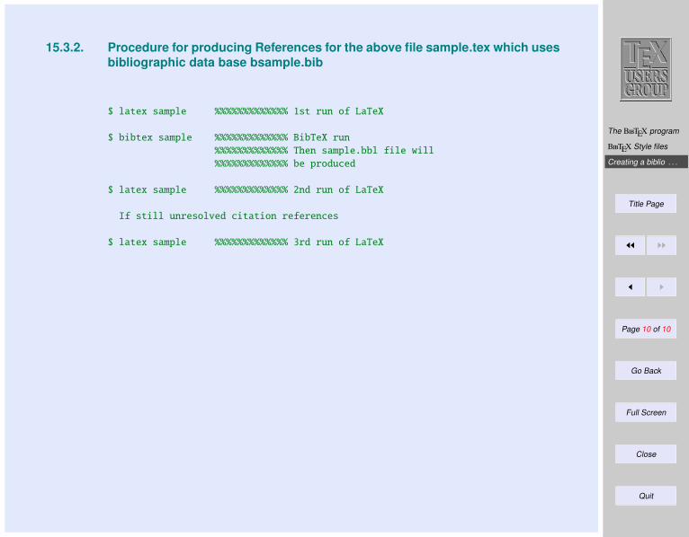
The BTEX program
BTEX Style files
Creating a biblio . . .
Title Page
JJ II
J I
Page 10 of 10
Go Back
Full Screen
Close
Quit
15.3.2. Procedure for producing References for the above file sample.tex which usesbibliographic data base bsample.bib
$ latex sample %%%%%%%%%%%%% 1st run of LaTeX
$ bibtex sample %%%%%%%%%%%%% BibTeX run
%%%%%%%%%%%%% Then sample.bbl file will
%%%%%%%%%%%%% be produced
$ latex sample %%%%%%%%%%%%% 2nd run of LaTeX
If still unresolved citation references
$ latex sample %%%%%%%%%%%%% 3rd run of LaTeX

Table of Contents
Index
Glossary
Title Page
JJ II
J I
Page 1 of 14
Go Back
Full Screen
Close
Quit
Indian TEX Users Group: http://www.river-valley.com/tug
16On-line Tutorial on LATEX
The Tutorial TeamIndian TEX Users Group, Buildings, Cotton Hills
Trivandrum 695014, 2000
Prof. (Dr.) K. S. S. Nambooripad, Director, Center for Mathematical Sciences, Trivandrum, (Editor); Dr. E. Krishnan, Readerin Mathematics, University College, Trivandrum; Mohit Agarwal, Department of Aerospace Engineering, Indian Institute of
Science, Bangalore; T. Rishi, Focal Image (India) Pvt. Ltd., Trivandrum; L. A. Ajith, Focal Image (India) Pvt. Ltd.,Trivandrum; A. M. Shan, Focal Image (India) Pvt. Ltd., Trivandrum; C. V. Radhakrishnan, River Valley Technologies,
Software Technology Park, Trivandrum constitute the Tutorial team
This document is generated from LATEX sources compiled with pdfLATEX v. 14e in an INTEL
Pentium III 700 MHz system running Linux kernel version 2.2.14-12. The packages usedare hyperref.sty and pdfscreen.sty
c©2000, Indian TEX Users Group. This document may be distributed under the terms of the LATEXProject Public License, as described in lppl.txt in the base LATEX distribution, either version 1.0
or, at your option, any later version
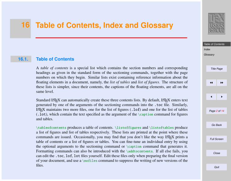
Table of Contents
Index
Glossary
Title Page
JJ II
J I
Page 2 of 14
Go Back
Full Screen
Close
Quit
16 Table of Contents, Index and Glossary
16.1. Table of Contents
A table of contents is a special list which contains the section numbers and correspondingheadings as given in the standard form of the sectioning commands, together with the pagenumbers on which they begin. Similar lists exist containing reference information about thefloating elements in a document, namely, the list of tables and list of figures. The structure ofthese lists is simpler, since their contents, the captions of the floating elements, are all on thesame level.
Standard LATEX can automatically create these three contents lists. By default, LATEX enters textgenerated by one of the arguments of the sectioning commands into the .toc file. Similarly,LATEX maintains two more files, one for the list of figures (.lof) and one for the list of tables(.lot), which contain the text specified as the argument of the \caption command for figuresand tables.
\tableofcontents produces a table of contents. \listoffigures and \listoftables producea list of figures and list of tables respectively. These lists are printed at the point where thesecommands are issued. Occasionally, you may find that you don’t like the way LATEX prints atable of contents or a list of figures or tables. You can fine-tune an individual entry by usingthe optional arguments to the sectioning command or \caption command that generates it.Formatting commands can also be introduced with the \addtocontents. If all else fails, youcan edit the .toc, lof, lot files yourself. Edit these files only when preparing the final versionof your document, and use a \nofiles command to suppress the writing of new versions of thefiles.
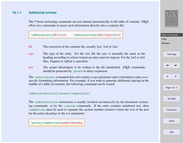
Table of Contents
Index
Glossary
Title Page
JJ II
J I
Page 3 of 14
Go Back
Full Screen
Close
Quit
16.1.1. Additional entries
The *-form sectioning commands are not entered automatically in the table of contents. LATEXoffers two commands to insert such information directly into a contents file:
\addtocontentsfiletext \addcontentslinefiletypetext
file The extension of the contents file, usually toc, lof or lot.
type The type of the entry. For the toc file the type is normally the same as theheading according to whose format an entry must be typeset. For the lof or lotfiles, figure or table is specified.
text The actual information to be written to the file mentioned. LATEX commandsshould be protected by \protect to delay expansion
The \addtocontents command does not contain a type parameter and is intended to enter user-specific formatting information. For example, if you want to generate additional spacing in themiddle of a table of contents, the following command can be issued:
\addtocontentstoc\protect\vspace2ex
The \addcontentsline instruction is usually invoked automatically by the document section-ing commands, or by the \caption commands. If the entry contains numbered text, then\numberline must be used to separate the section number (number) from the rest of the textfor the entry (heading) in the text parameter:
\protect\numberlinenumberheading
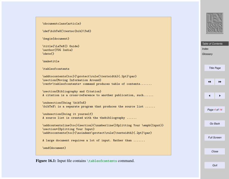
Table of Contents
Index
Glossary
Title Page
JJ II
J I
Page 4 of 14
Go Back
Full Screen
Close
Quit
\documentclassarticle
\def\bibTeX\textscbib\TeX
\begindocument
\title\LaTeX Guide
\authorTUG India
\date
\maketitle
\tableofcontents
\addtocontentstoc\protect\rule\textwidth.2pt\par
\sectionMoving Information Around
\verb+\tableofcontents+ command produces table of contents.......
\sectionBibliography and Citation
A citation is a cross-reference to another publication, such......
\subsectionUsing \bibTeX
\bibTeX\ is a separate program that produces the source list ......
\subsectionDoing it yourself
A source list is created with the thebibliography ......
\addcontentslinetocsection\numberlineSplitting Your \emphInput
\section*Splitting Your Input
\addtocontentstoc\noindent\protect\rule\textwidth.2pt\par
A large document requires a lot of input. Rather than .......
\enddocument
Figure 16.1: Input file contains \tableofcontents command.
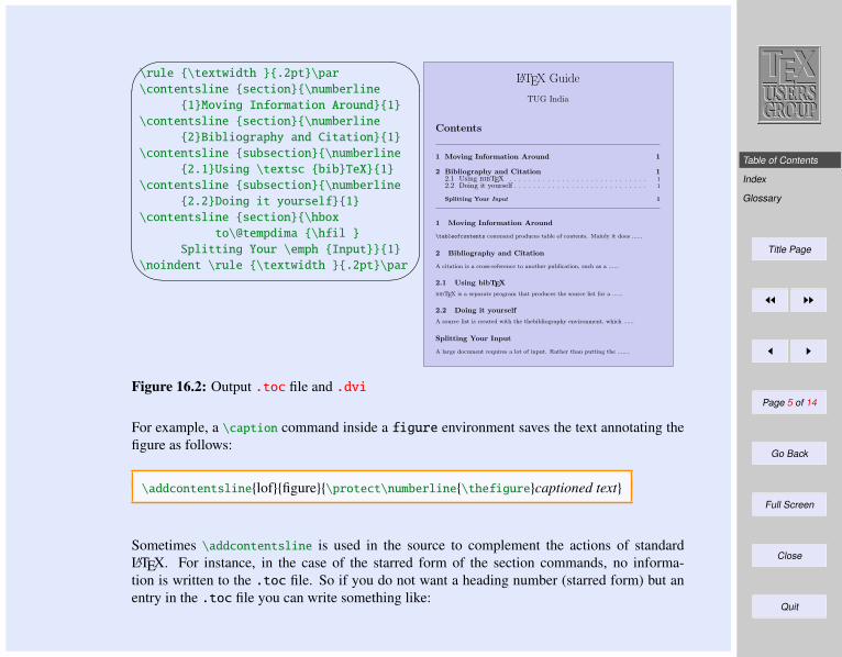
Table of Contents
Index
Glossary
Title Page
JJ II
J I
Page 5 of 14
Go Back
Full Screen
Close
Quit
'
&
$
%
\rule \textwidth .2pt\par
\contentsline section\numberline
1Moving Information Around1
\contentsline section\numberline
2Bibliography and Citation1
\contentsline subsection\numberline
2.1Using \textsc bibTeX1
\contentsline subsection\numberline
2.2Doing it yourself1
\contentsline section\hbox
to\@tempdima \hfil
Splitting Your \emph Input1
\noindent \rule \textwidth .2pt\par
LATEX Guide
TUG India
Contents
1 Moving Information Around 1
2 Bibliography and Citation 12.1 Using bibTEX . . . . . . . . . . . . . . . . . . . . . . . . . . . . . 12.2 Doing it yourself . . . . . . . . . . . . . . . . . . . . . . . . . . . . 1
Splitting Your Input 1
1 Moving Information Around
\tableofcontents command produces table of contents. Mainly it does ......
2 Bibliography and Citation
A citation is a cross-reference to another publication, such as a ......
2.1 Using bibTEXbibTEX is a separate program that produces the source list for a ......
2.2 Doing it yourselfA source list is created with the thebibliography environment, which ......
Splitting Your Input
A large document requires a lot of input. Rather than putting the .......
Figure 16.2: Output .toc file and .dvi
For example, a \caption command inside a figure environment saves the text annotating thefigure as follows:
\addcontentslineloffigure\protect\numberline\thefigurecaptioned text
Sometimes \addcontentsline is used in the source to complement the actions of standardLATEX. For instance, in the case of the starred form of the section commands, no informa-tion is written to the .toc file. So if you do not want a heading number (starred form) but anentry in the .toc file you can write something like:
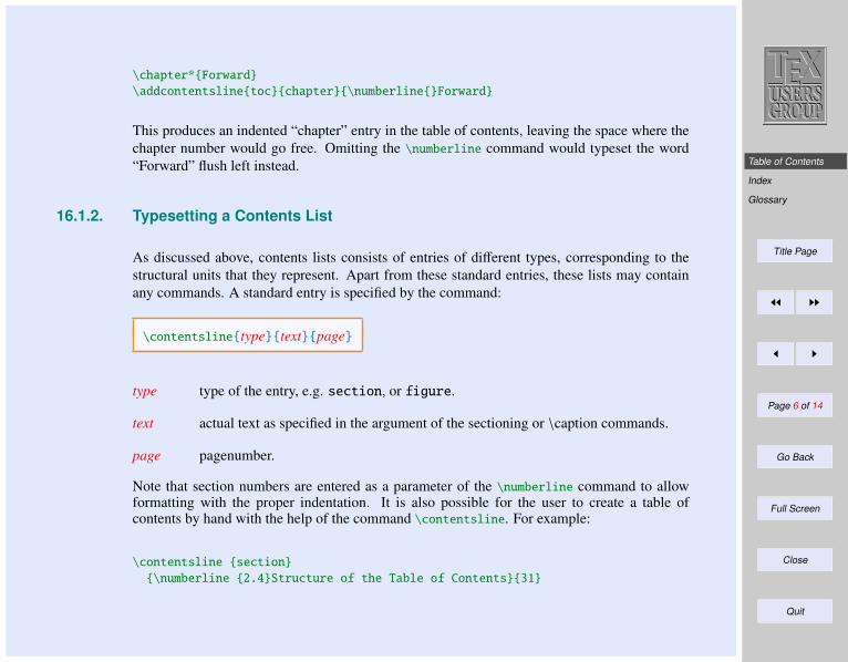
Table of Contents
Index
Glossary
Title Page
JJ II
J I
Page 6 of 14
Go Back
Full Screen
Close
Quit
\chapter*Forward
\addcontentslinetocchapter\numberlineForward
This produces an indented “chapter” entry in the table of contents, leaving the space where thechapter number would go free. Omitting the \numberline command would typeset the word“Forward” flush left instead.
16.1.2. Typesetting a Contents List
As discussed above, contents lists consists of entries of different types, corresponding to thestructural units that they represent. Apart from these standard entries, these lists may containany commands. A standard entry is specified by the command:
\contentslinetypetextpage
type type of the entry, e.g. section, or figure.
text actual text as specified in the argument of the sectioning or \caption commands.
page pagenumber.
Note that section numbers are entered as a parameter of the \numberline command to allowformatting with the proper indentation. It is also possible for the user to create a table ofcontents by hand with the help of the command \contentsline. For example:
\contentsline section
\numberline 2.4Structure of the Table of Contents31
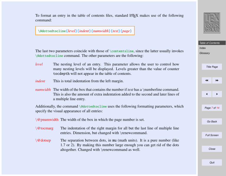
Table of Contents
Index
Glossary
Title Page
JJ II
J I
Page 7 of 14
Go Back
Full Screen
Close
Quit
To format an entry in the table of contents files, standard LATEX makes use of the followingcommand:
\@dottedtoclinelevelindentnumwidthtextpage
The last two parameters coincide with those of \contentsline, since the latter usually invokes\@dottedtocline command. The other parameters are the following:
level The nesting level of an entry. This parameter allows the user to control howmany nesting levels will be displayed. Levels greater than the value of countertocdepth will not appear in the table of contents.
indent This is total indentation from the left margin.
numwidth The width of the box that contains the number if text has a \numberline command.This is also the amount of extra indentation added to the second and later lines ofa multiple line entry.
Additionally, the command \@dottedtocline uses the following formatting parameters, whichspecify the visual appearance of all entries:
\@pnumwidth The width of the box in which the page number is set.
\@tocmarg The indentation of the right margin for all but the last line of multiple lineentries. Dimension, but changed with \renewcommand.
\@dotsep The separation between dots, in mu (math units). It is a pure number (like1.7 or 2). By making this number large enough you can get rid of the dotsaltogether. Changed with \renewcommand as well.
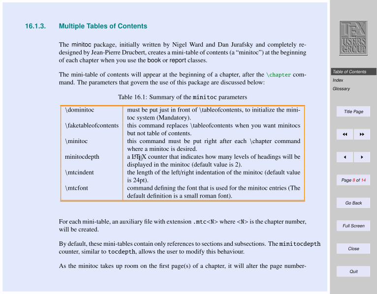
Table of Contents
Index
Glossary
Title Page
JJ II
J I
Page 8 of 14
Go Back
Full Screen
Close
Quit
16.1.3. Multiple Tables of Contents
The minitoc package, initially written by Nigel Ward and Dan Jurafsky and completely re-designed by Jean-Pierre Drucbert, creates a mini-table of contents (a “minitoc”) at the beginningof each chapter when you use the book or report classes.
The mini-table of contents will appear at the beginning of a chapter, after the \chapter com-mand. The parameters that govern the use of this package are discussed below:
Table 16.1: Summary of the minitoc parameters
\dominitoc must be put just in front of \tableofcontents, to initialize the mini-toc system (Mandatory).
\faketableofcontents this command replaces \tableofcontents when you want minitocsbut not table of contents.
\minitoc this command must be put right after each \chapter commandwhere a minitoc is desired.
minitocdepth a LATEX counter that indicates how many levels of headings will bedisplayed in the minitoc (default value is 2).
\mtcindent the length of the left/right indentation of the minitoc (default valueis 24pt).
\mtcfont command defining the font that is used for the minitoc entries (Thedefault definition is a small roman font).
For each mini-table, an auxiliary file with extension .mtc<N>where <N> is the chapter number,will be created.
By default, these mini-tables contain only references to sections and subsections. The minitocdepthcounter, similar to tocdepth, allows the user to modify this behaviour.
As the minitoc takes up room on the first page(s) of a chapter, it will alter the page number-

Table of Contents
Index
Glossary
Title Page
JJ II
J I
Page 9 of 14
Go Back
Full Screen
Close
Quit
ing. Therefore, three runs normally are needed to get correct information in the mini-table ofcontents.
To turn off the \minitoc commands, merely replace the package minitoc withminitocoff on your \usepackage command. This assures that all \minitoc commands willbe ignored.
16.2. Index
To find a topic of interest in a large document, book, or reference work, you usually turn to thetable of contents or, more often, to the index. Therefore, an index is a very important part of adocument, and most users’ entry point to a source of information is precisely through a pointerin the index. The most generally used index preparation program is MakeIndex
Each \index command causes LATEX to write an entry in the .idx file. This command writesthe text given as an argument, in the .idx file. This .idx will be generated only if we give\makeindex command in the preamble otherwise it will produce nothing.
\indexindex entry
To generate Index follow the procedure given below:
(1) Tag the words inside the document, which needs to come as index, as an argument of\index command.
(2) Include the makeidx package with an \usepackage command and put \makeindex com-mad at the preamble.
(3) Put a \printindex command where the index is to appear, normally before \enddocumentcommand.
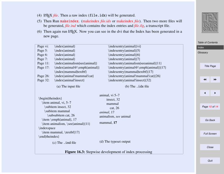
Table of Contents
Index
Glossary
Title Page
JJ II
J I
Page 10 of 14
Go Back
Full Screen
Close
Quit
(4) LATEX file. Then a raw index (file.idx) will be generated.(5) Then Run makeindex. (makeindex file.idx or makeindex file). Then two more files will
be generated, file.ind which contains the index entries and file.ilg, a transcript file.(6) Then again run LATEX. Now you can see in the dvi that the Index has been generated in a
new page.
Page vi: \indexanimalPage 5: \indexanimalPage 6: \indexanimalPage 7: \indexanimalPage 11: \indexanimalism|seeanimalPage 17: \indexanimal@\emphanimal
\indexmammal|textbfPage 26: \indexanimal!mammal!catPage 32: \indexanimal!insect
(a) The input file
\indexentryanimalvi\indexentryanimal5\indexentryanimal6\indexentryanimal7\indexentryanimalism|seeanimal11\indexentryanimal@\emphanimal17\indexentrymammal|textbf17\indexentryanimal!mammal!cat26\indexentryanimal!insect32
(b) The .idx file
\begintheindex\item animal, vi, 5–7\subitem insect, 32\subitem mammal\subsubitem cat, 26
\item \emphanimal, 17\item animalism, \seeanimal11\indexspace\item mammal, \textbf17\endtheindex
(c) The .ind file
animal, vi 5–7insect, 32mammal
cat, 26animal, 17animalism, see animal
mammal, 17
(d) The typeset output
Figure 16.3: Stepwise development of index processing
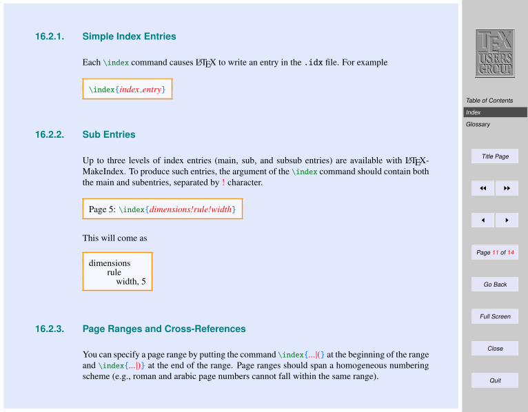
Table of Contents
Index
Glossary
Title Page
JJ II
J I
Page 11 of 14
Go Back
Full Screen
Close
Quit
16.2.1. Simple Index Entries
Each \index command causes LATEX to write an entry in the .idx file. For example
\indexindex entry
16.2.2. Sub Entries
Up to three levels of index entries (main, sub, and subsub entries) are available with LATEX-MakeIndex. To produce such entries, the argument of the \index command should contain boththe main and subentries, separated by ! character.
Page 5: \indexdimensions!rule!width
This will come as
dimensionsrule
width, 5
16.2.3. Page Ranges and Cross-References
You can specify a page range by putting the command \index...|( at the beginning of the rangeand \index...|) at the end of the range. Page ranges should span a homogeneous numberingscheme (e.g., roman and arabic page numbers cannot fall within the same range).
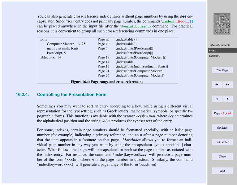
Table of Contents
Index
Glossary
Title Page
JJ II
J I
Page 12 of 14
Go Back
Full Screen
Close
Quit
You can also generate cross-reference index entries without page numbers by using the see en-capsulator. Since “see” entry does not print any page number, the commands \index...|see...can be placed anywhere in the input file after the \begindocument command. For practicalreasons, it is convenient to group all such cross-referencing commands in one place.
fontsComputer Modern, 13–25math, see math, fontsPostScript, 5
table, ii–xi, 14
Page ii: \indextable|(Page xi: \indextable|)Page 5: \indexfonts!PostScript|(
\indexfonts!PostScript|)Page 13 \indexfonts!Computer Modern |(Page 14: \indextablePage 17: \indexfonts!math|seemath, fontsPage 21: \indexfonts!Computer ModernPage 25: \indexfonts!Computer Modern|)
Figure 16.4: Page range and cross-referencing
16.2.4. Controlling the Presentation Form
Sometimes you may want to sort an entry according to a key, while using a different visualrepresentation for the typesetting, such as Greek letters, mathematical symbols, or specific ty-pographic forms. This function is available with the syntax: key@visual, where key determinesthe alphabetical position and the string value produces the typeset text of the entry.
For some, indexes, certain page numbers should be formatted specially, with an italic pagenumber (for example) indicating a primary reference, and an n after a page number denotingthat the item appears in a footnote on that page. MakeIndex allows you to format an indi-vidual page number in any way you want by using the encapsulator syntax specified | char-acter. What follows the | sign will “encapsulate” or enclose the page number associated withthe index entry. For instance, the command \indexkeyword|xxx will produce a page num-ber of the form \xxxn, where n is the page number in question. Similarly, the command\indexkeyword|(xxx) will generate a page range of the form \xxxn-m
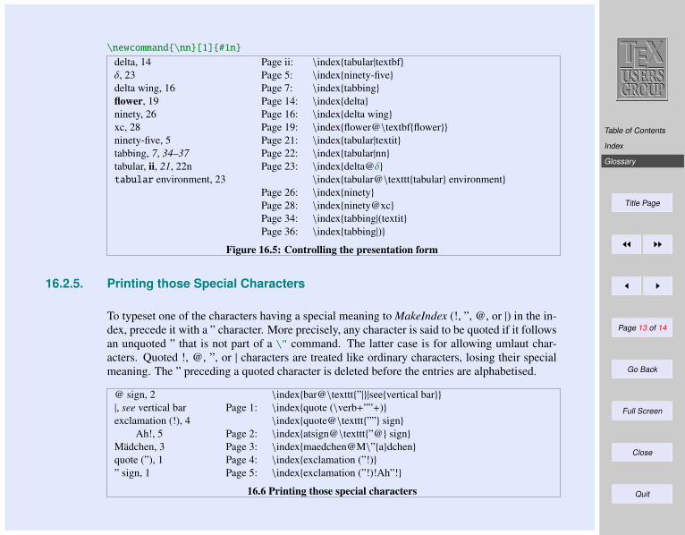
Table of Contents
Index
Glossary
Title Page
JJ II
J I
Page 13 of 14
Go Back
Full Screen
Close
Quit
\newcommand\nn[1]#1n
delta, 14δ, 23delta wing, 16flower, 19ninety, 26xc, 28ninety-five, 5tabbing, 7, 34–37tabular, ii, 21, 22ntabular environment, 23
Page ii: \indextabular|textbfPage 5: \indexninety-fivePage 7: \indextabbingPage 14: \indexdeltaPage 16: \indexdelta wingPage 19: \indexflower@\textbfflowerPage 21: \indextabular|textitPage 22: \indextabular|nnPage 23: \indexdelta@δ
\indextabular@\texttttabular environmentPage 26: \indexninetyPage 28: \indexninety@xcPage 34: \indextabbing|(textitPage 36: \indextabbing|)
Figure 16.5: Controlling the presentation form
16.2.5. Printing those Special Characters
To typeset one of the characters having a special meaning to MakeIndex (!, ”, @, or |) in the in-dex, precede it with a ” character. More precisely, any character is said to be quoted if it followsan unquoted ” that is not part of a \" command. The latter case is for allowing umlaut char-acters. Quoted !, @, ”, or | characters are treated like ordinary characters, losing their specialmeaning. The ” preceding a quoted character is deleted before the entries are alphabetised.
@ sign, 2|, see vertical barexclamation (!), 4
Ah!, 5Madchen, 3quote (”), 1” sign, 1
\indexbar@\texttt”||seevertical barPage 1: \indexquote (\verb+””+)
\indexquote@\texttt”” signPage 2: \indexatsign@\texttt”@ signPage 3: \indexmaedchen@M\”adchenPage 4: \indexexclamation (”!)Page 5: \indexexclamation (”!)!Ah”!
16.6 Printing those special characters
Table of Contents
Index
Glossary
Title Page
JJ II
J I
Page 14 of 14
Go Back
Full Screen
Close
Quit
16.3. Glossary
A ‘glossary’ is a special index of terms and phrases alphabetically ordered together with theirexplanations. To help set up a glossary, LATEX offers the commands
\makeglossary in the preamble and\glossaryglossary-entry in the text part
which function just like the commands for making up an index register. The entries are writtento a file with extension .glo after the command \makeglossary has been given in the preamble.The form of these file entries from each \glossary command is
\glossaryentryglossary-entrypagenumber
The information the .glo file can be used to establish a glossary. However, there is no equiva-lent to the theindex environment for a glossary, but a recommended structure is the descriptionenvironment or a special list environment.
Theorems in LATEX
Designer Theo . . .
Housekeeping
References
Title Page
JJ II
J I
Page 1 of 20
Go Back
Full Screen
Close
Quit
Indian TEX Users Group: http://www.river-valley.com/tug
17On-line Tutorial on LATEX
The Tutorial TeamIndian TEX Users Group, Buildings, Cotton Hills
Trivandrum 695014, 2000
Prof. (Dr.) K. S. S. Nambooripad, Director, Center for Mathematical Sciences, Trivandrum, (Editor); Dr. E. Krishnan, Readerin Mathematics, University College, Trivandrum; Mohit Agarwal, Department of Aerospace Engineering, Indian Institute of
Science, Bangalore; T. Rishi, Focal Image (India) Pvt. Ltd., Trivandrum; L. A. Ajith, Focal Image (India) Pvt. Ltd.,Trivandrum; A. M. Shan, Focal Image (India) Pvt. Ltd., Trivandrum; C. V. Radhakrishnan, River Valley Technologies,
Software Technology Park, Trivandrum constitute the Tutorial team
This document is generated from LATEX sources compiled with pdfLATEX v. 14e in an INTEL
Pentium III 700 MHz system running Linux kernel version 2.2.14-12. The packages usedare hyperref.sty and pdfscreen.sty
c©2000, Indian TEX Users Group. This document may be distributed under the terms of the LATEXProject Public License, as described in lppl.txt in the base LATEX distribution, either version 1.0
or, at your option, any later version
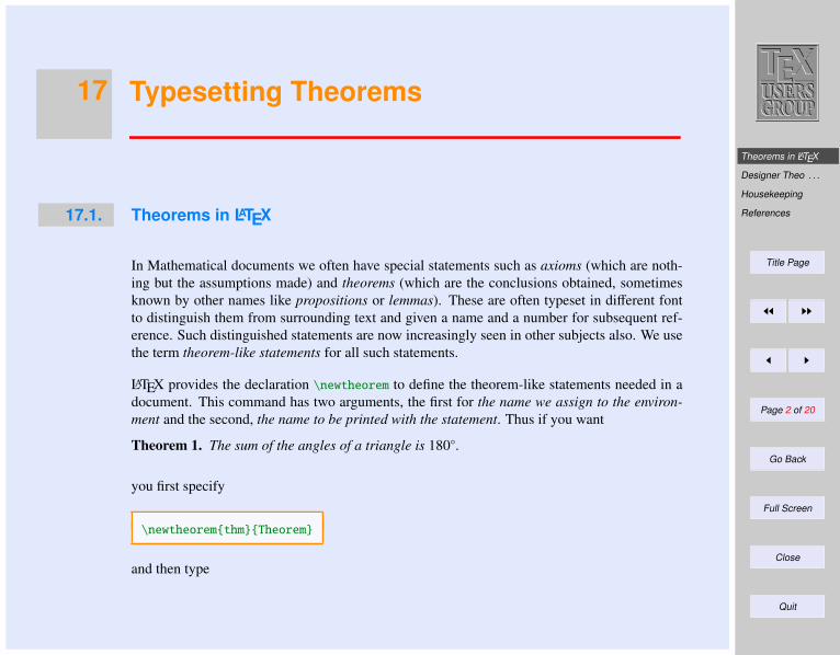
Theorems in LATEX
Designer Theo . . .
Housekeeping
References
Title Page
JJ II
J I
Page 2 of 20
Go Back
Full Screen
Close
Quit
17 Typesetting Theorems
17.1. Theorems in LATEX
In Mathematical documents we often have special statements such as axioms (which are noth-ing but the assumptions made) and theorems (which are the conclusions obtained, sometimesknown by other names like propositions or lemmas). These are often typeset in different fontto distinguish them from surrounding text and given a name and a number for subsequent ref-erence. Such distinguished statements are now increasingly seen in other subjects also. We usethe term theorem-like statements for all such statements.
LATEX provides the declaration \newtheorem to define the theorem-like statements needed in adocument. This command has two arguments, the first for the name we assign to the environ-ment and the second, the name to be printed with the statement. Thus if you want
Theorem 1. The sum of the angles of a triangle is 180.
you first specify
\newtheoremthmTheorem
and then type
Theorems in LATEX
Designer Theo . . .
Housekeeping
References
Title Page
JJ II
J I
Page 3 of 20
Go Back
Full Screen
Close
Quit
\beginthm
The sum of the angles of a triangle is $180ˆ\circ$.
\endthm
Note that in the command \newtheorem the first argument can be any name you fancy, insteadof the thm given here. Also, it is a good idea to keep all your \newtheorem commands togetherin the preamble.
The \newtheorem command has a couple of optional arguments which control the way the cor-responding statement is numbered. For example if you want the above theorem to be numbered1.1 (the first theorem of the first section) rather than a plain 1, then you must specify
\newtheoremthmTheorem[section]
in the \newtheorem command. Then the same input as above for the theorem produces
Theorem 17.1.1. The sum of the angles of a triangle is 180.
The next Theorem will be numbered 1.2, the third Theorem in the fourth section will be num-bered 4.3 and so on.
The other optional argument of the \newtheorem command is useful when you have severaldifferent types of theorem-like statements (such as lemmas and corollaries) and you want someof them to share the same numbering sequence. For example if you want
Theorem 17.1.2. The sum of the angles of a triangle is 180.
An immediate consequence of the result is the following
Corollary 17.1.3. The sum of the angles of a quadrilateral is 360.
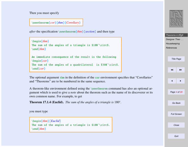
Theorems in LATEX
Designer Theo . . .
Housekeeping
References
Title Page
JJ II
J I
Page 4 of 20
Go Back
Full Screen
Close
Quit
Then you must specify
\newtheoremcor[thm]Corollary
after the specification \newtheoremthm[section] and then type
\beginthm
The sum of the angles of a triangle is $180ˆ\circ$.
\endthm
An immediate consequence of the result is the following
\begincorThe sum of the angles of a quadrilateral is $360ˆ\circ$.
\endcor
The optional argument thm in the definition of the cor environment specifies that “Corollaries”and “Theorems” are to be numbered in the same sequence.
A theorem-like environment defined using the \newtheorem command has also an optional ar-gument which is used to give a note about the theorem such as the name of its discoverer or itsown common name. For example, to get
Theorem 17.1.4 (Euclid). The sum of the angles of a triangle is 180.
you must type
\beginthm[Euclid]The sum of the angles of a triangle is $180ˆ\circ$.
\endthm
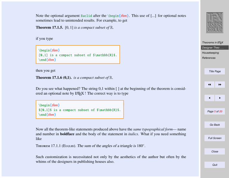
Theorems in LATEX
Designer Theo . . .
Housekeeping
References
Title Page
JJ II
J I
Page 5 of 20
Go Back
Full Screen
Close
Quit
Note the optional argument Euclid after the \beginthm. This use of [...] for optional notessometimes lead to unintended results. For example, to get
Theorem 17.1.5. [0, 1] is a compact subset of R.
if you type
\beginthm
[0,1] is a compact subset of $\mathbbR$.
\endthm
then you get
Theorem 17.1.6 (0,1). is a compact subset of R.
Do you see what happened? The string 0,1 within [ ] at the beginning of the theorem is consid-ered an optional note by LATEX ! The correct way is to type
\beginthm
$[0,1]$ is a compact subset of $\mathbbR$.
\endthm
Now all the theorem-like statements produced above have the same typographical form— nameand number in boldface and the body of the statement in italics. What if you need somethinglike
T 17.1.1 (E). The sum of the angles of a triangle is 180.
Such customization is necessitated not only by the aesthetics of the author but often by thewhims of the designers in publishing houses also.
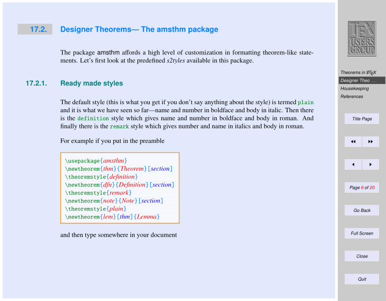
Theorems in LATEX
Designer Theo . . .
Housekeeping
References
Title Page
JJ II
J I
Page 6 of 20
Go Back
Full Screen
Close
Quit
17.2. Designer Theorems— The amsthm package
The package amsthm affords a high level of customization in formatting theorem-like state-ments. Let’s first look at the predefined s2tyles available in this package.
17.2.1. Ready made styles
The default style (this is what you get if you don’t say anything about the style) is termed plain
and it is what we have seen so far—name and number in boldface and body in italic. Then thereis the definition style which gives name and number in boldface and body in roman. Andfinally there is the remark style which gives number and name in italics and body in roman.
For example if you put in the preamble
\usepackageamsthm
\newtheoremthmTheorem[section]\theoremstyledefinition\newtheoremdfnDefinition[section]\theoremstyleremark\newtheoremnoteNote[section]\theoremstyleplain\newtheoremlem[thm]Lemma
and then type somewhere in your document
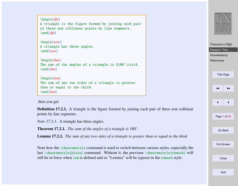
Theorems in LATEX
Designer Theo . . .
Housekeeping
References
Title Page
JJ II
J I
Page 7 of 20
Go Back
Full Screen
Close
Quit
\begindfnA triangle is the figure formed by joining each pair
of three non collinear points by line segments.
\enddfn
\beginnoteA triangle has three angles.
\endnote
\beginthm
The sum of the angles of a triangle is $180ˆ\circ$.
\endthm
\beginlem
The sum of any two sides of a triangle is greater
than or equal to the third.
\endlem
then you get
Definition 17.2.1. A triangle is the figure formed by joining each pair of three non collinearpoints by line segments.
Note 17.2.1. A triangle has three angles.
Theorem 17.2.1. The sum of the angles of a triangle is 180.
Lemma 17.2.2. The sum of any two sides of a triangle is greater than or equal to the third.
Note how the \theoremstyle command is used to switch between various styles, especially thelast \theoremstyleplain command. Without it, the previous \theoremstyleremark willstill be in force when lem is defined and so “Lemma” will be typeset in the remark style.
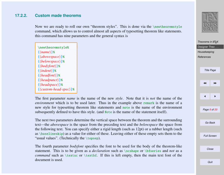
Theorems in LATEX
Designer Theo . . .
Housekeeping
References
Title Page
JJ II
J I
Page 8 of 20
Go Back
Full Screen
Close
Quit
17.2.2. Custom made theorems
Now we are ready to roll our own “theorem styles”. This is done via the \newtheoremstyle
command, which allows us to control almost all aspects of typesetting theorem like statements.this command has nine parameters and the general syntax is
\newtheoremstyle%
〈name〉%〈abovespace〉%〈belowspace〉%〈bodyfont〉%〈indent〉%〈headfont〉%〈headpunct〉%〈headspace〉%〈custom-head-spec〉%
The first parameter name is the name of the new style. Note that it is not the name of theenvironment which is to be used later. Thus in the example above remark is the name of anew style for typesetting theorem like statements and note is the name of the environmentsubsequently defined to have this style. (and Note is the name of the statement itself).
The next two parameters determine the vertical space between the theorem and the surroundingtext—the abovespace is the space from the preceding text and the belowspace the space fromthe following text. You can specify either a rigid length (such as 12pt) or a rubber length (suchas \baselineskip) as a value for either of these. Leaving either of these empty sets them to the“usual values”. (Technically the \topsep).
The fourth parameter bodyfont specifies the font to be used for the body of the theorem-likestatement. This is to be given as a declaration such as \scshape or \bfseries and not as acommand such as \textsc or \textbf. If this is left empty, then the main text font of thedocument is used.
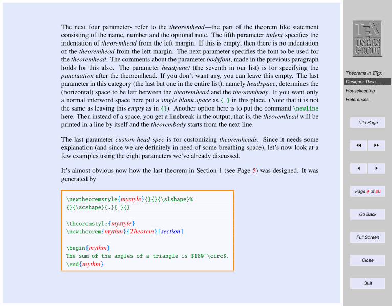
Theorems in LATEX
Designer Theo . . .
Housekeeping
References
Title Page
JJ II
J I
Page 9 of 20
Go Back
Full Screen
Close
Quit
The next four parameters refer to the theoremhead—the part of the theorem like statementconsisting of the name, number and the optional note. The fifth parameter indent specifies theindentation of theoremhead from the left margin. If this is empty, then there is no indentationof the theoremhead from the left margin. The next parameter specifies the font to be used forthe theoremhead. The comments about the parameter bodyfont, made in the previous paragraphholds for this also. The parameter headpunct (the seventh in our list) is for specifying thepunctuation after the theoremhead. If you don’t want any, you can leave this empty. The lastparameter in this category (the last but one in the entire list), namely headspace, determines the(horizontal) space to be left between the theoremhead and the theorembody. If you want onlya normal interword space here put a single blank space as in this place. (Note that it is notthe same as leaving this empty as in ). Another option here is to put the command \newline
here. Then instead of a space, you get a linebreak in the output; that is, the theoremhead will beprinted in a line by itself and the theorembody starts from the next line.
The last parameter custom-head-spec is for customizing theoremheads. Since it needs someexplanation (and since we are definitely in need of some breathing space), let’s now look at afew examples using the eight parameters we’ve already discussed.
It’s almost obvious now how the last theorem in Section 1 (see Page 5) was designed. It wasgenerated by
\newtheoremstylemystyle\slshape%\scshape.
\theoremstylemystyle\newtheoremmythmTheorem[section]
\beginmythm
The sum of the angles of a triangle is $180ˆ\circ$.
\endmythm
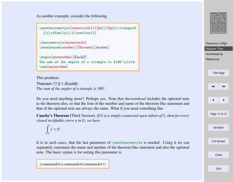
Theorems in LATEX
Designer Theo . . .
Housekeeping
References
Title Page
JJ II
J I
Page 10 of 20
Go Back
Full Screen
Close
Quit
As another example, consider the following
\newtheoremstylemynewstyle12pt12pt\itshape%\sffamily:\newline
\theoremstylemynewstyle\newtheoremmythmTheorem[section]
\beginmynewthm[Euclid]The sum of the angles of a triangle is $180ˆ\circ$.
\endmynewthm
This producesTheorem 17.2.1 (Euclid):The sum of the angles of a triangle is 180.
Do you need anything more? Perhaps yes. Note that theoremhead includes the optional noteto the theorem also, so that the font of the number and name of the theorem-like statement andthat of the optional note are always the same. What if you need something like
Cauchy’s Theorem (Third Version). If G is a simply connected open subset of C, then for everyclosed rectifiable curve γ in G, we have∫
γ
f = 0
It is in such cases, that the last parameter of \newtheoremstyle is needed. Using it we canseparately customize the name and number of the theorem-like statement and also the optionalnote. The basic syntax is for setting this parameter is
commands#1commands#2commands#3
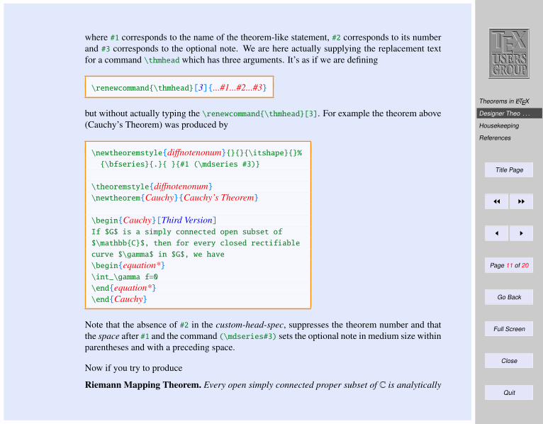
Theorems in LATEX
Designer Theo . . .
Housekeeping
References
Title Page
JJ II
J I
Page 11 of 20
Go Back
Full Screen
Close
Quit
where #1 corresponds to the name of the theorem-like statement, #2 corresponds to its numberand #3 corresponds to the optional note. We are here actually supplying the replacement textfor a command \thmhead which has three arguments. It’s as if we are defining
\renewcommand\thmhead[3]...#1...#2...#3
but without actually typing the \renewcommand\thmhead[3]. For example the theorem above(Cauchy’s Theorem) was produced by
\newtheoremstylediffnotenonum\itshape%
\bfseries. #1 (\mdseries #3)
\theoremstylediffnotenonum
\newtheoremCauchyCauchy’s Theorem
\beginCauchy[Third Version]If $G$ is a simply connected open subset of
$\mathbbC$, then for every closed rectifiable
curve $\gamma$ in $G$, we have
\beginequation*\int_\gamma f=0
\endequation*\endCauchy
Note that the absence of #2 in the custom-head-spec, suppresses the theorem number and thatthe space after #1 and the command (\mdseries#3) sets the optional note in medium size withinparentheses and with a preceding space.
Now if you try to produce
Riemann Mapping Theorem. Every open simply connected proper subset of C is analytically
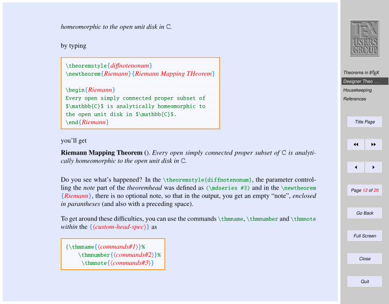
Theorems in LATEX
Designer Theo . . .
Housekeeping
References
Title Page
JJ II
J I
Page 12 of 20
Go Back
Full Screen
Close
Quit
homeomorphic to the open unit disk in C.
by typing
\theoremstylediffnotenonum
\newtheoremRiemannRiemann Mapping THeorem
\beginRiemannEvery open simply connected proper subset of
$\mathbbC$ is analytically homeomorphic to
the open unit disk in $\mathbbC$.
\endRiemann
you’ll get
Riemann Mapping Theorem (). Every open simply connected proper subset of C is analyti-cally homeomorphic to the open unit disk in C.
Do you see what’s happened? In the \theoremstylediffnotenonum, the parameter control-ling the note part of the theoremhead was defined as (\mdseries #3) and in the \newtheorem
Riemann, there is no optional note, so that in the output, you get an empty “note”, enclosedin parantheses (and also with a preceding space).
To get around these difficulties, you can use the commands \thmname, \thmnumber and \thmnote
within the 〈custom-head-spec〉 as
\thmname〈commands#1〉%\thmnumber〈commands#2〉%\thmnote〈commands#3〉
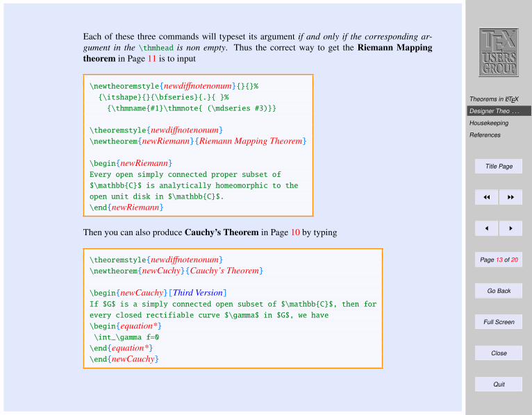
Theorems in LATEX
Designer Theo . . .
Housekeeping
References
Title Page
JJ II
J I
Page 13 of 20
Go Back
Full Screen
Close
Quit
Each of these three commands will typeset its argument if and only if the corresponding ar-gument in the \thmhead is non empty. Thus the correct way to get the Riemann Mappingtheorem in Page 11 is to input
\newtheoremstylenewdiffnotenonum%
\itshape\bfseries. %
\thmname#1\thmnote (\mdseries #3)
\theoremstylenewdiffnotenonum
\newtheoremnewRiemannRiemann Mapping Theorem
\beginnewRiemannEvery open simply connected proper subset of
$\mathbbC$ is analytically homeomorphic to the
open unit disk in $\mathbbC$.
\endnewRiemann
Then you can also produce Cauchy’s Theorem in Page 10 by typing
\theoremstylenewdiffnotenonum
\newtheoremnewCuchyCauchy’s Theorem
\beginnewCauchy[Third Version]If $G$ is a simply connected open subset of $\mathbbC$, then for
every closed rectifiable curve $\gamma$ in $G$, we have
\beginequation*\int_\gamma f=0
\endequation*\endnewCauchy
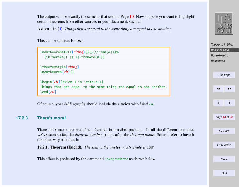
Theorems in LATEX
Designer Theo . . .
Housekeeping
References
Title Page
JJ II
J I
Page 14 of 20
Go Back
Full Screen
Close
Quit
The output will be exactly the same as that seen in Page 10. Now suppose you want to highlightcertain theorems from other sources in your document, such as
Axiom 1 in [1]. Things that are equal to the same thing are equal to one another.
This can be done as follows
\newtheoremstyleciting\itshape%\bfseries. \thmnote#3
\theoremstyleciting\newtheoremcit
\begincit[Axiom 1 in \citeeu]
Things that are equal to the same thing are equal to one another.
\endcit
Of course, your bibliography should include the citation with label eu.
17.2.3. There’s more!
There are some more predefined features in amsthm package. In all the different exampleswe’ve seen so far, the theorem number comes after the theorem name. Some prefer to have itthe other way round as in
17.2.1. Theorem (Euclid). The sum of the angles in a triangle is 180
This effect is produced by the command \swapnumbers as shown below
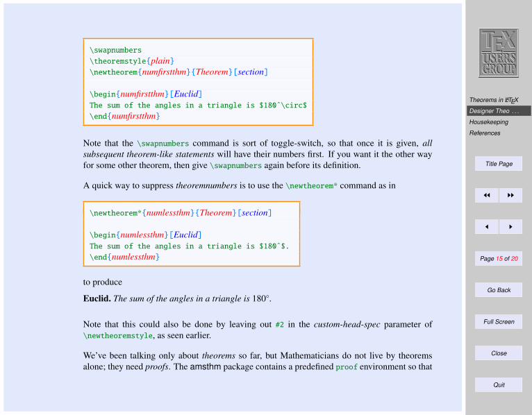
Theorems in LATEX
Designer Theo . . .
Housekeeping
References
Title Page
JJ II
J I
Page 15 of 20
Go Back
Full Screen
Close
Quit
\swapnumbers
\theoremstyleplain\newtheoremnumfirstthmTheorem[section]
\beginnumfirstthm[Euclid]The sum of the angles in a triangle is $180ˆ\circ$
\endnumfirstthm
Note that the \swapnumbers command is sort of toggle-switch, so that once it is given, allsubsequent theorem-like statements will have their numbers first. If you want it the other wayfor some other theorem, then give \swapnumbers again before its definition.
A quick way to suppress theoremnumbers is to use the \newtheorem* command as in
\newtheorem*numlessthmTheorem[section]
\beginnumlessthm[Euclid]The sum of the angles in a triangle is $180ˆ$.
\endnumlessthm
to produce
Euclid. The sum of the angles in a triangle is 180.
Note that this could also be done by leaving out #2 in the custom-head-spec parameter of\newtheoremstyle, as seen earlier.
We’ve been talking only about theorems so far, but Mathematicians do not live by theoremsalone; they need proofs. The amsthm package contains a predefined proof environment so that
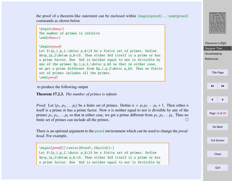
Theorems in LATEX
Designer Theo . . .
Housekeeping
References
Title Page
JJ II
J I
Page 16 of 20
Go Back
Full Screen
Close
Quit
the proof of a theorem-like statement can be enclosed within \beginproof...\endproof
commands as shown below
\beginthmsecThe number of primes is infinite
\endthmsec
\beginproofLet $\p_1,p_2,\dotsc p_k\$ be a finite set of primes. Define
$n=p_1p_2\dotsm p_k+1$. Then either $n$ itself is a prime or has
a prime factor. Now $n$ is neither equal to nor is divisible by
any of the primes $p_1,p_2,\dotsc p_k$ so that in either case,
we get a prime different from $p_1,p_2\dotsc p_k$. Thus no finite
set of primes includes all the primes.
\endproof
to produce the following output
Theorem 17.2.3. The number of primes is infinite
Proof. Let p1, p2, . . . pk be a finite set of primes. Define n = p1 p2 · · · pk + 1. Then either nitself is a prime or has a prime factor. Now n is neither equal to nor is divisible by any of theprimes p1, p2, . . . pk so that in either case, we get a prime different from p1, p2 . . . pk. Thus nofinite set of primes can include all the primes.
There is an optional argument to the proof environment which can be used to change the proof-head. For example,
\beginproof[\textscProof\,(Euclid):]Let $\p_1,p_2,\dotsc p_k\$ be a finite set of primes. Define
$n=p_1p_2\dotsm p_k+1$. Then either $n$ itself is a prime or has
a prime factor. Now $n$ is neither equal to nor is divisible by
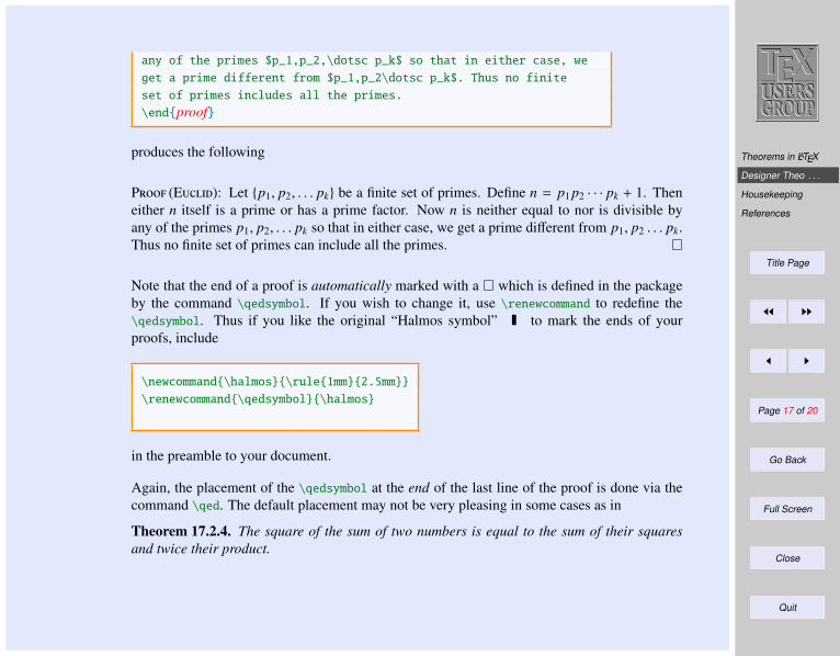
Theorems in LATEX
Designer Theo . . .
Housekeeping
References
Title Page
JJ II
J I
Page 17 of 20
Go Back
Full Screen
Close
Quit
any of the primes $p_1,p_2,\dotsc p_k$ so that in either case, we
get a prime different from $p_1,p_2\dotsc p_k$. Thus no finite
set of primes includes all the primes.
\endproof
produces the following
P (E): Let p1, p2, . . . pk be a finite set of primes. Define n = p1 p2 · · · pk + 1. Theneither n itself is a prime or has a prime factor. Now n is neither equal to nor is divisible byany of the primes p1, p2, . . . pk so that in either case, we get a prime different from p1, p2 . . . pk.Thus no finite set of primes can include all the primes.
Note that the end of a proof is automatically marked with a which is defined in the packageby the command \qedsymbol. If you wish to change it, use \renewcommand to redefine the\qedsymbol. Thus if you like the original “Halmos symbol” to mark the ends of yourproofs, include
\newcommand\halmos\rule1mm2.5mm
\renewcommand\qedsymbol\halmos
in the preamble to your document.
Again, the placement of the \qedsymbol at the end of the last line of the proof is done via thecommand \qed. The default placement may not be very pleasing in some cases as in
Theorem 17.2.4. The square of the sum of two numbers is equal to the sum of their squaresand twice their product.
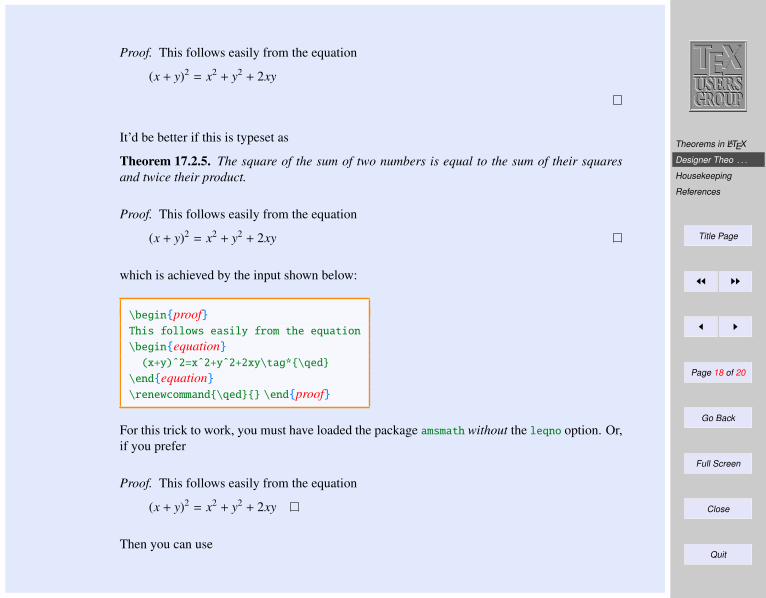
Theorems in LATEX
Designer Theo . . .
Housekeeping
References
Title Page
JJ II
J I
Page 18 of 20
Go Back
Full Screen
Close
Quit
Proof. This follows easily from the equation
(x + y)2 = x2 + y2 + 2xy
It’d be better if this is typeset as
Theorem 17.2.5. The square of the sum of two numbers is equal to the sum of their squaresand twice their product.
Proof. This follows easily from the equation
(x + y)2 = x2 + y2 + 2xy
which is achieved by the input shown below:
\beginproofThis follows easily from the equation
\beginequation(x+y)ˆ2=xˆ2+yˆ2+2xy\tag*\qed
\endequation\renewcommand\qed \endproof
For this trick to work, you must have loaded the package amsmath without the leqno option. Or,if you prefer
Proof. This follows easily from the equation
(x + y)2 = x2 + y2 + 2xy
Then you can use
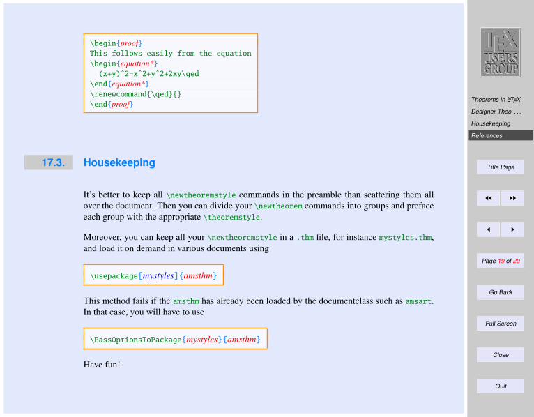
Theorems in LATEX
Designer Theo . . .
Housekeeping
References
Title Page
JJ II
J I
Page 19 of 20
Go Back
Full Screen
Close
Quit
\beginproofThis follows easily from the equation
\beginequation*(x+y)ˆ2=xˆ2+yˆ2+2xy\qed
\endequation*\renewcommand\qed
\endproof
17.3. Housekeeping
It’s better to keep all \newtheoremstyle commands in the preamble than scattering them allover the document. Then you can divide your \newtheorem commands into groups and prefaceeach group with the appropriate \theoremstyle.
Moreover, you can keep all your \newtheoremstyle in a .thm file, for instance mystyles.thm,and load it on demand in various documents using
\usepackage[mystyles]amsthm
This method fails if the amsthm has already been loaded by the documentclass such as amsart.In that case, you will have to use
\PassOptionsToPackagemystylesamsthm
Have fun!
Theorems in LATEX
Designer Theo . . .
Housekeeping
References
Title Page
JJ II
J I
Page 20 of 20
Go Back
Full Screen
Close
Quit
17.4. References
[1] Euclid, The Elements, Greece 300 BC