1

Friday, November 02, 2007

Estimates of State Price Levels for Consumption Goods and Services: a first brush∗

Bettina H. Aten

Introduction This paper develops exploratory estimates of the spatial price differences for consumption goods and services at the U.S. state level. Spatial (place-to-place) price differences are important to regional and other sub-national accounting frameworks as they make possible comparisons of economic data that are adjusted for geographic differences in price levels. In international comparisons, these adjustments are termed purchasing power parities (PPP); when divided by exchange rates they are called national price levels. In areas with a common currency like the Euro, the exchange rates are the same and the PPP becomes the price level. Just as there are differences in price levels between European Union member countries, there are significant differences in the purchasing power of a currency across diverse areas of the United States, for example between metropolitan New York compared to rural South Dakota. I use the term Spatial Price Indexes (SPIs) to label these sub-national estimates of PPPs. The SPIs can be used to adjust consumption-related statistics, such as per capita incomes, expenditures and output, providing users with a more accurate picture of regional economic differences at one point in time. The SPIs are built up in this paper from two main data sets. The first is the principal source of consumer price information in the United States, the Bureau of Labor Statistics Consumer Price Index (CPI) for 38 metropolitan and urban areas, which is of course a time-to-time index. Aten (2006) presented spatial price index estimates for 2003 and 2004 for these 38 areas, which cover 87% of the population but only about 15% of U.S. counties. In addition, some states are not covered at all by the CPI. The second source of information is the county level rent surveys from the U.S. Census Bureau. The estimates presented here are generated using a multi-stage approach that bridges the results in the areas sampled by the CPI price surveys to the remaining non-sampled areas using the Census rent information.

General description The background to this paper is the work detailed in Aten (2005, 2006) on estimating place-to-place indexes for 38 metropolitan and urban areas in 2003 and 2004. These indexes are termed spatial price indexes (SPI) to distinguish them from the Consumer Price Index (CPI) that tracks changes over time in one place. The CPI survey is designed to cover a fixed set of geographical areas, so that SPIs can only be directly estimated at ∗ Bettina H. Aten is an economist in the Regional Economics Directorate, Bureau of Economic Analysis. The results presented here are the responsibility of the author and not of the Bureau of Economic Analysis. Email: Bettina.Aten@bea.gov

2

this 38 metropolitan and urban area level. More disaggregated calculations or more extensive geographical coverage would require a redesign of the CPI survey, something that is not feasible in the short run. Given that there are significant differences in price levels for the metropolitan and urban areas covered by the CPI, there is much interest in a) adjusting economic data to reflect these price differences, such as when making comparisons of income levels and expenditure levels (Bernstein et al [2000], Johnson et al [2001]) and b) assessing the feasibility of estimating SPIs for different geographies, such as states and regions (see for example Fuchs et al [1979], Ball and Fenwick [2004], Roos [2006]). Any such use involves making inferences for areas not sampled by the CPI. One problem in making these inferences is the change of scale that arises in aggregations that are different from the observed levels, for example, from metro area to counties or from metro areas to states. A related problem is that some of the CPI areas cross state lines, while others refer to single counties1. For example, the District of Columbia is only one of 26 counties in the Greater Washington metropolitan area as defined in the CPI, but it is also a quasi state, or at least, for many purposes, a separate entity from the states of Virginia or Maryland. Los Angeles is one county and one CPI area by itself, but only one of 58 counties in the state of California. The CPI area termed South B (medium and small urban areas in the South Region), is made up of 84 smaller units, scattered across states such as Georgia, Tennessee, and South Carolina. Combining and using these disparate spatial units is problematic for a number of reasons. The approach applied here is to break down these areas into somewhat less heterogeneous units, namely counties, then build up the county data back into state level estimates. The second main issue is the lack of data for a great number of areas. We know from the survey design of the CPI that these non-sampled areas are systematically excluded because of their smaller, less dense populations and lower volumes of expenditures. This means that direct inferences from the sampled areas of the CPI to the non-sampled areas would be misleading because the distribution of expenditures and prices are also likely to be systematically different. The second stage of this paper aims to bridge the gap between the sampled and non-sampled CPI areas indirectly, using data on rental price levels from the 2000 Census. The consequences of scale, classification inconsistencies and sampling coverage that characterize these data have been discussed in the spatial statistical literature (Goodchild, Anselin and Deichmann [1993], Gotway and Young [2002], Baneerje and Gelfand [2004], Anselin and Gallo [2006]). In the social sciences, issues in spatial aggregation are known as the ecological fallacy problem and the modifiable areal unit problem. Anselin (2002), among others, extensively reviews the conceptual and practical consequences for applied spatial models in the econometric literature.

1 Some areas refer to townships within counties. The term county in this paper refers to counties and county equivalents, plus the 78 municipalities of Puerto Rico. More details on the geographical boundaries can be found in the next section.

3

The methods adopted here attempt to mitigate, not resolve, some of the major estimating problems associated with changes of scale and spatial aggregation, but are by necessity data-driven. They are summarized below and then discussed more extensively in subsequent sections. The estimation of the spatial price indexes (SPIs) at the state level is divided into three stages. The first takes the 38 CPI areas and decomposes them into smaller and more consistent geographical areas, generally counties. The relationship between the average price levels for these areas and the observed county rents are modeled, and price levels are predicted for the individual counties within the 38 CPI areas. The second stage involves bridging these predictions to the remaining counties in the U.S. that are not in the CPI sample, counties which tend to be in primarily non-metropolitan and rural areas. It is subdivided into two steps, the first one assigns initial values to all counties, while the second one again relies heavily on the modeled relationship between price levels and rents, which are observed for all U.S. counties covered by the Census, including those not in the CPI sample. The final stage builds up the aggregate state price levels based on these estimated county price levels, and tests the sensitivity of these results to alternative specifications.

Background on the Data

Interarea Price Levels and Census Rents The methodology for estimating SPIs for the 38 metropolitan and urban areas of the CPI has been detailed in Aten (2005, 2006) using 2003 and 2004 prices. It includes estimating a weighted hedonic regression for each expenditure item that make up consumer goods and services in the U.S., a total of about 400 items. These range from rents and new automobiles to shoes and haircuts. The hedonic regressions take into account item characteristics, such as unit size and packaging, as well as the location and type of outlet where it is sold, and uses probability sampling quotes as weights. The resulting item price levels are then aggregated into major categories, such as Food and Beverages, Transportation, and Housing, and up to an overall SPI for consumption, using item expenditure weights at the 38 area level (see Appendix Table A1 for a list of all counties comprising these areas). The 2000 Census rents consist of monthly rental estimates at seven levels of geographic aggregation, three definitions of units, and five bedroom size categories. The non-cash rental units were excluded in this study. The recent movers are included, defined as having moved within the last two years. These rental observations are averaged geometrically across five bedroom size categories: from zero to four bedrooms, weighted by the number of units in each category. The Census data include state, county, metropolitan area, place and county subdivision code, thus permitting a good geographical matching to the BLS Consumer Price Index (CPI) data. The 38 CPI areas

4

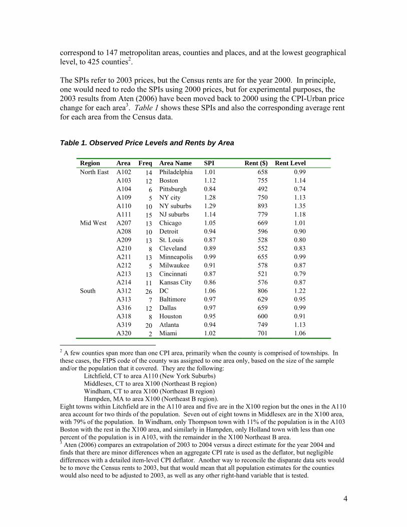
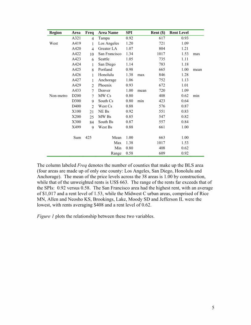
correspond to 147 metropolitan areas, counties and places, and at the lowest geographical level, to 425 counties2. The SPIs refer to 2003 prices, but the Census rents are for the year 2000. In principle, one would need to redo the SPIs using 2000 prices, but for experimental purposes, the 2003 results from Aten (2006) have been moved back to 2000 using the CPI-Urban price change for each area3. Table 1 shows these SPIs and also the corresponding average rent for each area from the Census data.

Table 1. Observed Price Levels and Rents by Area

Region Area Freq Area Name SPI Rent ($) Rent Level North East A102 14 Philadelphia 1.01 658 0.99 A103 12 Boston 1.12 755 1.14 A104 6 Pittsburgh 0.84 492 0.74 A109 5 NY city 1.28 750 1.13 A110 10 NY suburbs 1.29 893 1.35 A111 15 NJ suburbs 1.14 779 1.18 Mid West A207 13 Chicago 1.05 669 1.01 A208 10 Detroit 0.94 596 0.90 A209 13 St. Louis 0.87 528 0.80 A210 8 Cleveland 0.89 552 0.83 A211 13 Minneapolis 0.99 655 0.99 A212 5 Milwaukee 0.91 578 0.87 A213 13 Cincinnati 0.87 521 0.79 A214 11 Kansas City 0.86 576 0.87 South A312 26 DC 1.06 806 1.22 A313 7 Baltimore 0.97 629 0.95 A316 12 Dallas 0.97 659 0.99 A318 8 Houston 0.95 600 0.91 A319 20 Atlanta 0.94 749 1.13 A320 2 Miami 1.02 701 1.06

2 A few counties span more than one CPI area, primarily when the county is comprised of townships. In these cases, the FIPS code of the county was assigned to one area only, based on the size of the sample and/or the population that it covered. They are the following:

Litchfield, CT to area A110 (New York Suburbs) Middlesex, CT to area X100 (Northeast B region) Windham, CT to area X100 (Northeast B region) Hampden, MA to area X100 (Northeast B region).

Eight towns within Litchfield are in the A110 area and five are in the X100 region but the ones in the A110 area account for two thirds of the population. Seven out of eight towns in Middlesex are in the X100 area, with 79% of the population. In Windham, only Thompson town with 11% of the population is in the A103 Boston with the rest in the X100 area, and similarly in Hampden, only Holland town with less than one percent of the population is in A103, with the remainder in the X100 Northeast B area. 3 Aten (2006) compares an extrapolation of 2003 to 2004 versus a direct estimate for the year 2004 and finds that there are minor differences when an aggregate CPI rate is used as the deflator, but negligible differences with a detailed item-level CPI deflator. Another way to reconcile the disparate data sets would be to move the Census rents to 2003, but that would mean that all population estimates for the counties would also need to be adjusted to 2003, as well as any other right-hand variable that is tested.

5

Region Area Freq Area Name SPI Rent ($) Rent Level A321 4 Tampa 0.92 617 0.93 West A419 1 Los Angeles 1.20 721 1.09 A420 4 Greater LA 1.07 804 1.21 A422 10 San Francisco 1.34 1017 1.53 max A423 6 Seattle 1.05 735 1.11 A424 1 San Diego 1.14 783 1.18 A425 8 Portland 0.98 665 1.00 mean A426 1 Honolulu 1.38 max 846 1.28 A427 1 Anchorage 1.06 752 1.13 A429 2 Phoenix 0.93 672 1.01 A433 7 Denver 1.00 mean 720 1.09 Non-metro D200 7 MW Cs 0.80 408 0.62 min D300 9 South Cs 0.80 min 423 0.64 D400 2 West Cs 0.88 576 0.87 X100 21 NE Bs 0.92 551 0.83 X200 25 MW Bs 0.85 547 0.82 X300 84 South Bs 0.87 557 0.84 X499 9 West Bs 0.88 661 1.00

Sum 425 Mean 1.00 663 1.00 Max 1.38 1017 1.53 Min 0.80 408 0.62 Range 0.58 609 0.92

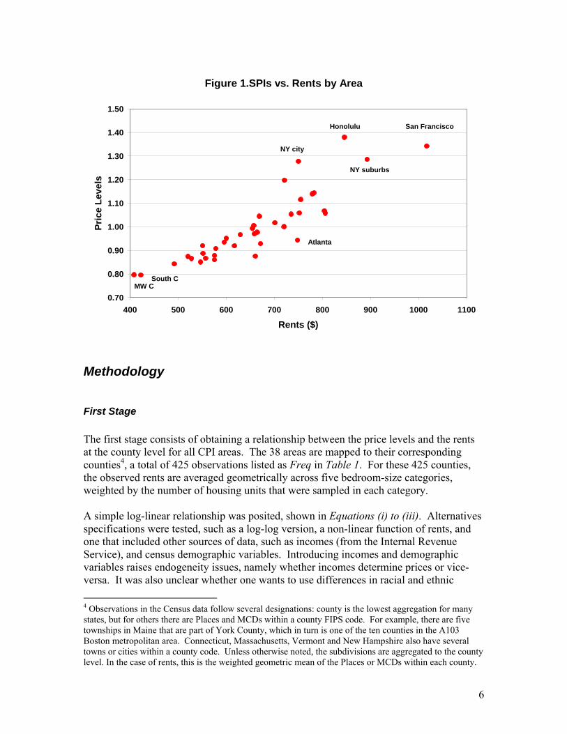
The column labeled Freq denotes the number of counties that make up the BLS area (four areas are made up of only one county: Los Angeles, San Diego, Honolulu and Anchorage). The mean of the price levels across the 38 areas is 1.00 by construction, while that of the unweighted rents is US$ 663. The range of the rents far exceeds that of the SPIs: 0.92 versus 0.58. The San Francisco area had the highest rent, with an average of $1,017 and a rent level of 1.53, while the Midwest C urban areas, comprised of Rice MN, Allen and Neosho KS, Brookings, Lake, Moody SD and Jefferson IL were the lowest, with rents averaging $408 and a rent level of 0.62. Figure 1 plots the relationship between these two variables.

6

Methodology

First Stage The first stage consists of obtaining a relationship between the price levels and the rents at the county level for all CPI areas. The 38 areas are mapped to their corresponding counties4, a total of 425 observations listed as Freq in Table 1. For these 425 counties, the observed rents are averaged geometrically across five bedroom-size categories, weighted by the number of housing units that were sampled in each category. A simple log-linear relationship was posited, shown in Equations (i) to (iii). Alternatives specifications were tested, such as a log-log version, a non-linear function of rents, and one that included other sources of data, such as incomes (from the Internal Revenue Service), and census demographic variables. Introducing incomes and demographic variables raises endogeneity issues, namely whether incomes determine prices or vice-versa. It was also unclear whether one wants to use differences in racial and ethnic 4 Observations in the Census data follow several designations: county is the lowest aggregation for many states, but for others there are Places and MCDs within a county FIPS code. For example, there are five townships in Maine that are part of York County, which in turn is one of the ten counties in the A103 Boston metropolitan area. Connecticut, Massachusetts, Vermont and New Hampshire also have several towns or cities within a county code. Unless otherwise noted, the subdivisions are aggregated to the county level. In the case of rents, this is the weighted geometric mean of the Places or MCDs within each county.

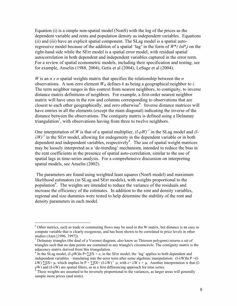
Figure 1.SPIs vs. Rents by Area

0.70

0.80

0.90

1.00

1.10

1.20

1.30

1.40

1.50

400 500 600 700 800 900 1000 1100

Rents ($)

Pric

e Le

vels

San FranciscoHonolulu

MW CSouth C

NY suburbs

Atlanta

NY city

7

make-up to control for geographic price differences5. Since the objective is not to explain price levels, but rather to obtain estimates based on their correlation to price indicators that have a more extensive geographical coverage, it was felt that these variables should not be included, and only rents and population densities were retained as independent variables.

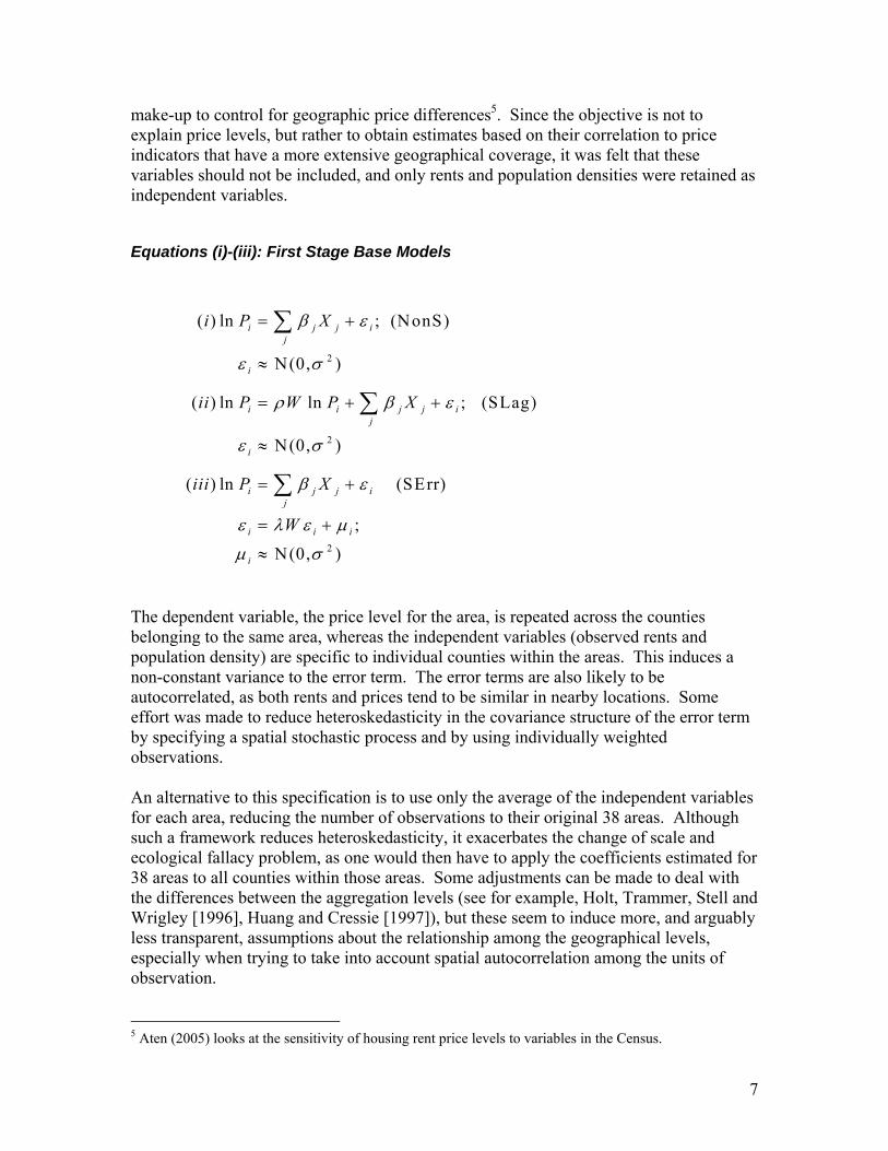
Equations (i)-(iii): First Stage Base Models

The dependent variable, the price level for the area, is repeated across the counties belonging to the same area, whereas the independent variables (observed rents and population density) are specific to individual counties within the areas. This induces a non-constant variance to the error term. The error terms are also likely to be autocorrelated, as both rents and prices tend to be similar in nearby locations. Some effort was made to reduce heteroskedasticity in the covariance structure of the error term by specifying a spatial stochastic process and by using individually weighted observations. An alternative to this specification is to use only the average of the independent variables for each area, reducing the number of observations to their original 38 areas. Although such a framework reduces heteroskedasticity, it exacerbates the change of scale and ecological fallacy problem, as one would then have to apply the coefficients estimated for 38 areas to all counties within those areas. Some adjustments can be made to deal with the differences between the aggregation levels (see for example, Holt, Trammer, Stell and Wrigley [1996], Huang and Cressie [1997]), but these seem to induce more, and arguably less transparent, assumptions about the relationship among the geographical levels, especially when trying to take into account spatial autocorrelation among the units of observation. 5 Aten (2005) looks at the sensitivity of housing rent price levels to variables in the Census.

2

2

2

( ) ln ; (NonS)

N(0, )

( ) ln ln ; (SLag)

N(0, )

( ) ln (SErr)

;

N(0, )

i j j ij

i

i i j j ij

i

i j j ij

i i i

i

i P X

ii P W P X

iii P X

W

β ε

ε σ

ρ β ε

ε σ

β ε

ε λ ε μ

μ σ

= +

≈

= + +

≈

= +

= +

≈

∑

∑

∑

8

Equation (i) is a simple non-spatial model (NonS) with the log of the prices as the dependent variable and rents and population density as independent variables. Equations (ii) and (iii) have an explicit spatial component. The SLag model is a spatial auto-regressive model because of the addition of a spatial ‘lag’ in the form of W*( lnPi) on the right-hand side while the SErr model is a spatial error model, with residual spatial autocorrelation in both dependent and independent variables captured in the error term. For a review of spatial econometric models, including their specification and testing, see for example, Anselin (1988, 2004), Getis et al (2004), LeSage et al (2004). W is an n x n spatial weights matrix that specifies the relationship between the n observations. A non-zero element Wik defines k as being a geographical neighbor to i. The term neighbor ranges in this context from nearest neighbors, to contiguity, to inverse distance matrix definitions of neighbors. For example, a first-order nearest neighbor matrix will have ones in the row and columns corresponding to observations that are closest to each other geographically, and zero otherwise6. Inverse distance matrices will have entries in all the elements (except the main diagonal) indicating the inverse of the distance between the observations. The contiguity matrix is defined using a Delaunay triangulation7, with observations having from three to twelve neighbors. One interpretation of W is that of a spatial multiplier, (I-ρW)-1 in the SLag model and (I-λW)-1 in the SErr model, allowing for endogeneity in the dependent variable or in both dependent and independent variables, respectively8. The use of spatial weight matrices may be loosely interpreted as a ‘de-trending’ mechanism, intended to reduce the bias in the rent coefficients in the presence of spatial auto-correlation, similar to the use of spatial lags in time-series analysis. For a comprehensive discussion on interpreting spatial models, see Anselin (2002). The parameters are found using weighted least squares (NonS model) and maximum likelihood estimators (in SLag and SErr models), with weights proportional to the population9. The weights are intended to reduce the variance of the residuals and increase the efficiency of the estimates. In addition to the rent and density variables, regional and size dummies were tested to help determine the stability of the rent and density parameters in each model.

6 Other metrics, such as trade or commuting flows may be used in the W matrix, but distance is an easy to compute variable that is clearly exogenous, and has been shown to be correlated to price levels in other studies (Aten [1996, 1997]). 7 Delaunay triangles (the dual of a Voronoi diagram, also know as Thiessen polygons) returns a set of triangles such that no data points are contained in any triangle's circumcircle. The contiguity matrix is the adjacency matrix derived from this triangulation. 8 In the SLag model, (I-ρW)ln P=∑βX + ε; in the SErr model, the ‘lag’ applies to both dependent and independent variables – translating into the error term after some algebraic manipulation: (I-λW)ln P =(I-λW) ∑βX+ μ, which implies ln P = ∑βX+ (I-λW)-1 μ, with ε= λW ε + μ. Another interpretation is that (I-ρW) and (I-λW) are spatial filters, as in a first differencing approach for time series. 9 These weights are assumed to be inversely proportional to the variances, as larger areas will generally sample more prices (and rents).

9

The results of the ‘best’ model in each of the three specifications are presented in the Results section, but numerous variations were tested, and a summary of the sensitivity of the estimates to different combinations of spatial weights matrices W is shown at the end of the paper. The predicted individual county price levels are normalized so that their weighted average equals the average price level for the area. That is, the weighted averages of the within-area county price levels equal the original observed input price levels.

Second Stage The second stage involves bridging the predicted price levels in the 425 counties from the previous stage to all U.S. counties that are covered by the Census, including areas not sampled by the CPI. This is done in several steps. For ease of exposition, the 425 counties that constitute the 38 areas sampled by the CPI are denoted ‘overlap’ counties because they are in both the BLS CPI sample data and the Census rental data. The areas not sampled in the CPI are denoted ‘census only’ counties. Together, the overlap and census-only counties cover the 3219 counties. First, the ratio of the weighted geometric mean of rents in census-only areas to overlap areas is calculated. This ratio is then multiplied by the weighted geometric average of the price levels in the counties predicted in Stage One. In Equations (iv), ‘over’ refers to overlap counties, while ‘census’ refers to counties only in the Census rent sample. The weights refer to population weights. For example, in Missouri, the rent ratio is 0.87, with fifteen counties that overlap averaging $540 in rents and 172 counties only in the census averaging $468. This ratio is then multiplied by the weighted geometric average of the price levels in the fifteen counties predicted in the first stage (0.86). For Missouri, this includes eight counties in St. Louis (A209) and seven in Kansas City (A214). The result, 0.75, is an average estimated price level for the remaining non-sampled 172 counties in Missouri.

Equations (iv): Bridge Ratios

( )

where exp( ln )

exp( ln ),

*

where exp( ln

census overlap

census j j jj census j census

overlap i i ii overlap i overlap

census overlap

overlap i ii overlap

Ratio Rent Rent

Rent w Rent w

Rent w Rent w

PL PL Ratio

PL w PL

∈ ∈

∈ ∈

∈

=

=

=

=

=

∑ ∑

∑ ∑

∑ )ii overlap

w∈∑

10

The process is repeated for all states, with the exception of states that have no overlap at all. These are Iowa, Montana, New Mexico, North Dakota, Rhode Island, Wyoming and Puerto Rico10, where a higher geographical aggregation, the division, is used instead of the state. There are nine divisions, their average rents and ratios are listed in Table 3 in the Results section. The bridged price level estimates from Equation (iv) become the dependent variables in the second stage regression model. It mirrors the first stage regressions in that the estimated price levels for each county enter as dependent variables, and are repeated across areas bridged by the same ratio. The actual individual rents as well as observed population densities for each county are the independent variables. The observations are weighted in proportion to the population. A weighted least squares formulation is tested (NonS) as well as two spatial models– the spatial lag (SLag) and the spatial error (SErr) models, identical in form to Equations (i) to (iii) depicted earlier. As in the first stage, different spatial weight matrices are used but instead of 425 observations, n increases to 3219, corresponding to all uniquely identified FIPS county codes in the Census rent data.

Final Stage The final stage estimates the State Price Indexes or SPIs using the weighted geometric average of the predicted county values from the previous step. Ideally one would use expenditure weights but these are not available below the 38 area level, so population weights are used. The results are described in more detail below, followed by a discussion of their sensitivity to various specifications.

Results

First Stage Results The first stage estimation results consist of the three basic equations: a non-spatial (NonS) formulation and two spatial (SLag and SErr) models. The independent variables are the rents and the population density. The base models shown in Table 2 have separate regional intercept dummies. Alternative constraints and combinations were tested, including twelve different weight matrices (Ws) for each formulation. These are discussed in more detail in the Sensitivity section.

10 Puerto Rico is included in this study even though it is a territory and not a state as it has a full set of sampled rents for its 78 municipalities.

11

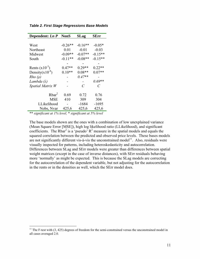
Table 2. First Stage Regressions Base Models Dependent: Ln P NonS SLag SErr West -0.26** -0.16** -0.05* Northeast 0.01 -0.01 -0.03 Midwest -0.09** -0.07** -0.15**South -0.11** -0.08** -0.15** - - - Rents (x10-3) 0.47** 0.29** 0.22** Density(x10-4) 0.10** 0.08** 0.07** Rho (ρ) - 0.47** - Lambda (λ) - - 0.69** Spatial Matrix W - C C

Rbar2 0.69 0.72 0.76 MSE 410 309 304

LLikelihood - -1684 -1695 Nobs, Nvar 425,6 425,6 425,6

** significant at 1% level, * significant at 5% level The base models shown are the ones with a combination of low unexplained variance (Mean Square Error [MSE]), high log likelihood ratio (LLikelihood), and significant coefficients. The Rbar2 is a ‘pseudo’ R2 measure in the spatial models and equals the squared correlation between the predicted and observed price levels. These bases models are not significantly different vis-à-vis the unconstrained model11. Also, residuals were visually inspected for patterns, including heteroskedasticity and autocorrelation. Differences between SLag and SErr models were greater than differences between spatial weight matrices (except in the case of inverse distances), with SErr residuals behaving more ‘normally’ as might be expected. This is because the SLag models are correcting for the autocorrelation of the dependent variable, but not adjusting for the autocorrelation in the rents or in the densities as well, which the SErr model does.

11 The F-test with (3, 425) degrees of freedom for the semi-constrained versus the unconstrained model in all cases averaged 2.0.

12

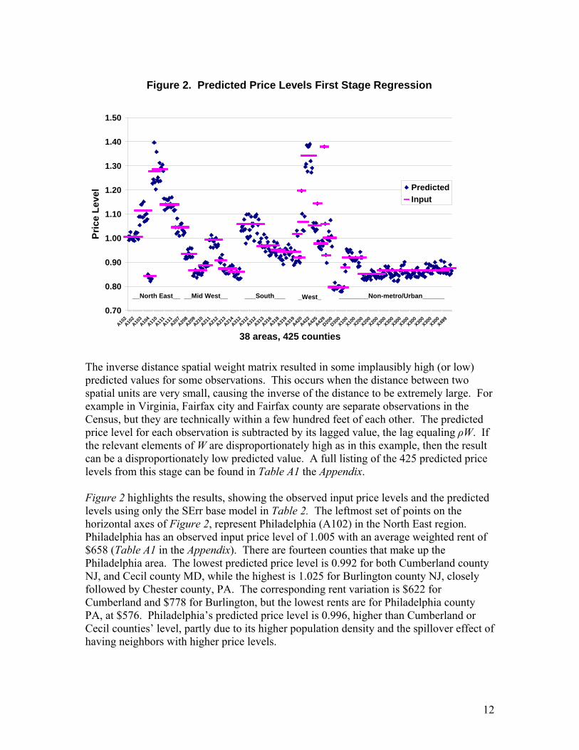
The inverse distance spatial weight matrix resulted in some implausibly high (or low) predicted values for some observations. This occurs when the distance between two spatial units are very small, causing the inverse of the distance to be extremely large. For example in Virginia, Fairfax city and Fairfax county are separate observations in the Census, but they are technically within a few hundred feet of each other. The predicted price level for each observation is subtracted by its lagged value, the lag equaling ρW. If the relevant elements of W are disproportionately high as in this example, then the result can be a disproportionately low predicted value. A full listing of the 425 predicted price levels from this stage can be found in Table A1 the Appendix. Figure 2 highlights the results, showing the observed input price levels and the predicted levels using only the SErr base model in Table 2. The leftmost set of points on the horizontal axes of Figure 2, represent Philadelphia (A102) in the North East region. Philadelphia has an observed input price level of 1.005 with an average weighted rent of $658 (Table A1 in the Appendix). There are fourteen counties that make up the Philadelphia area. The lowest predicted price level is 0.992 for both Cumberland county NJ, and Cecil county MD, while the highest is 1.025 for Burlington county NJ, closely followed by Chester county, PA. The corresponding rent variation is $622 for Cumberland and $778 for Burlington, but the lowest rents are for Philadelphia county PA, at $576. Philadelphia’s predicted price level is 0.996, higher than Cumberland or Cecil counties’ level, partly due to its higher population density and the spillover effect of having neighbors with higher price levels.

Figure 2. Predicted Price Levels First Stage Regression

0.70

0.80

0.90

1.00

1.10

1.20

1.30

1.40

1.50

A102A10

2A10

3A10

4A11

0A11

1A11

1A20

7A20

8A20

9A21

0A21

1A21

2A21

3A21

4A31

2A31

2A31

2A31

3A31

6A31

8A31

9A31

9A42

0A42

2A42

5A42

9D20

0D30

0X10

0X10

0X20

0X20

0X20

0X30

0X30

0X30

0X30

0X30

0X30

0X30

0X30

0X49

9

38 areas, 425 counties

Pric

e Le

vel Predicted

Input

__North East__ __Mid West__ ___South___ _West_ ________Non-metro/Urban______

13

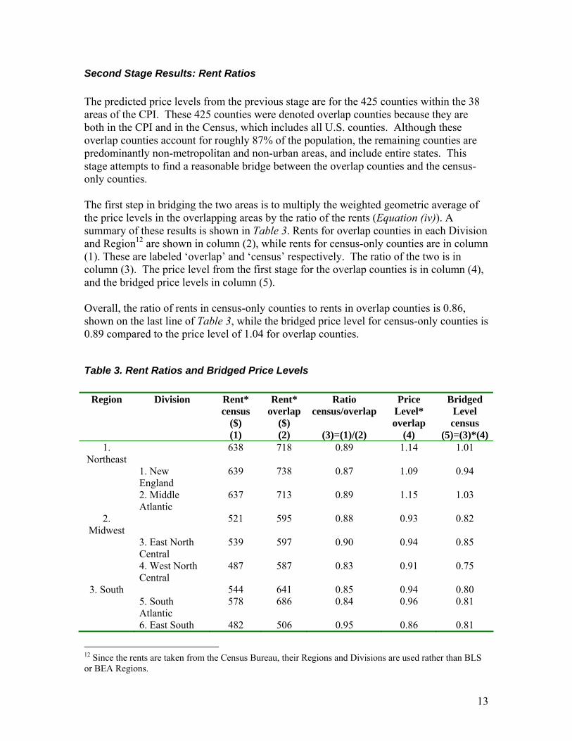
Second Stage Results: Rent Ratios The predicted price levels from the previous stage are for the 425 counties within the 38 areas of the CPI. These 425 counties were denoted overlap counties because they are both in the CPI and in the Census, which includes all U.S. counties. Although these overlap counties account for roughly 87% of the population, the remaining counties are predominantly non-metropolitan and non-urban areas, and include entire states. This stage attempts to find a reasonable bridge between the overlap counties and the census-only counties. The first step in bridging the two areas is to multiply the weighted geometric average of the price levels in the overlapping areas by the ratio of the rents (Equation (iv)). A summary of these results is shown in Table 3. Rents for overlap counties in each Division and Region12 are shown in column (2), while rents for census-only counties are in column (1). These are labeled ‘overlap’ and ‘census’ respectively. The ratio of the two is in column (3). The price level from the first stage for the overlap counties is in column (4), and the bridged price levels in column (5). Overall, the ratio of rents in census-only counties to rents in overlap counties is 0.86, shown on the last line of Table 3, while the bridged price level for census-only counties is 0.89 compared to the price level of 1.04 for overlap counties.

Table 3. Rent Ratios and Bridged Price Levels

Region Division Rent* census

($) (1)

Rent* overlap

($) (2)

Ratio census/overlap

(3)=(1)/(2)

Price Level* overlap

(4)

Bridged Level census

(5)=(3)*(4) 1.

Northeast 638 718 0.89 1.14 1.01

1. New England

639 738 0.87 1.09 0.94

2. Middle Atlantic

637 713 0.89 1.15 1.03

2. Midwest

521 595 0.88 0.93 0.82

3. East North Central

539 597 0.90 0.94 0.85

4. West North Central

487 587 0.83 0.91 0.75

3. South 544 641 0.85 0.94 0.80 5. South

Atlantic 578 686 0.84 0.96 0.81

6. East South 482 506 0.95 0.86 0.81

12 Since the rents are taken from the Census Bureau, their Regions and Divisions are used rather than BLS or BEA Regions.

14

Region Division Rent* census

($) (1)

Rent* overlap

($) (2)

Ratio census/overlap

(3)=(1)/(2)

Price Level* overlap

(4)

Bridged Level census

(5)=(3)*(4) Central

7. West South Central

532 592 0.90 0.93 0.84

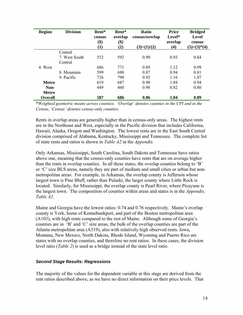
4. West 686 771 0.89 1.12 0.99 8. Mountain 599 688 0.87 0.94 0.81 9. Pacific 726 790 0.92 1.16 1.07

Metro 619 687 0.90 1.04 0.94 Non-

Metro 449 460 0.98 0.82 0.80

Overall 587 686 0.86 1.04 0.89 *Weighted geometric means across counties. ‘Overlap’ denotes counties in the CPI and in the Census, ‘Census’ denotes census-only counties. Rents in overlap areas are generally higher than in census-only areas. The highest rents are in the Northeast and West, especially in the Pacific division that includes California, Hawaii, Alaska, Oregon and Washington. The lowest rents are in the East South Central division comprised of Alabama, Kentucky, Mississippi and Tennessee. The complete list of state rents and ratios is shown in Table A2 in the Appendix. Only Arkansas, Mississippi, South Carolina, South Dakota and Tennessee have ratios above one, meaning that the census-only counties have rents that are on average higher than the rents in overlap counties. In all these states, the overlap counties belong to ‘B’ or ‘C’ size BLS areas, namely they are part of medium and small cities or urban but non-metropolitan areas. For example, in Arkansas, the overlap county is Jefferson whose largest town is Pine Bluff, rather than Pulaski, the larger county where Little Rock is located. Similarly, for Mississippi, the overlap county is Pearl River, where Picayune is the largest town. The composition of counties within areas and states is in the Appendix, Table A1. Maine and Georgia have the lowest ratios: 0.74 and 0.76 respectively. Maine’s overlap county is York, home of Kennebunkport, and part of the Boston metropolitan area (A103), with high rents compared to the rest of Maine. Although some of Georgia’s counties are in ‘B’ and ‘C’ size areas, the bulk of the overlap counties are part of the Atlanta metropolitan area (A319), also with relatively high observed rents. Iowa, Montana, New Mexico, North Dakota, Rhode Island, Wyoming and Puerto Rico are states with no overlap counties, and therefore no rent ratios. In these cases, the division level ratio (Table 2) is used as a bridge instead of the state level ratio.

Second Stage Results: Regressions The majority of the values for the dependent variable in this stage are derived from the rent ratios described above, as we have no direct information on their price levels. That

15

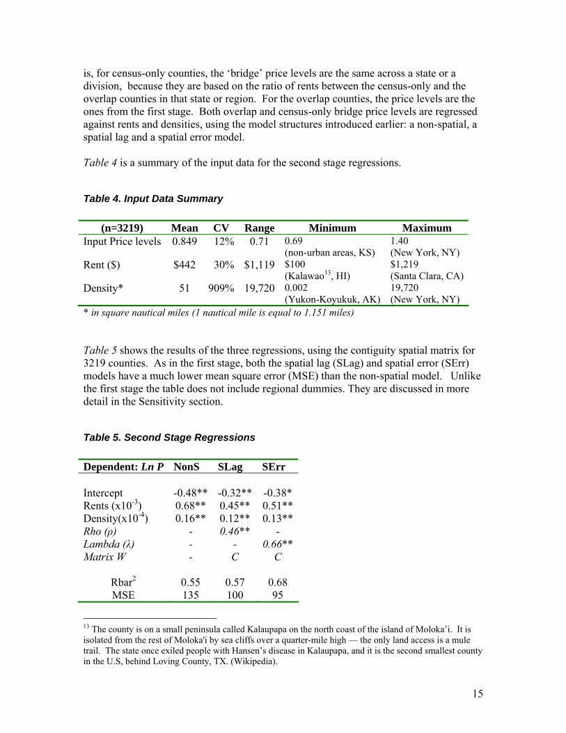
is, for census-only counties, the ‘bridge’ price levels are the same across a state or a division, because they are based on the ratio of rents between the census-only and the overlap counties in that state or region. For the overlap counties, the price levels are the ones from the first stage. Both overlap and census-only bridge price levels are regressed against rents and densities, using the model structures introduced earlier: a non-spatial, a spatial lag and a spatial error model. Table 4 is a summary of the input data for the second stage regressions.

Table 4. Input Data Summary

(n=3219) Mean CV Range Minimum Maximum Input Price levels 0.849 12% 0.71 0.69

(non-urban areas, KS) 1.40 (New York, NY)

Rent ($) $442 30% $1,119 $100 (Kalawao13, HI)

$1,219 (Santa Clara, CA)

Density* 51 909% 19,720 0.002 (Yukon-Koyukuk, AK)

19,720 (New York, NY)

* in square nautical miles (1 nautical mile is equal to 1.151 miles)

Table 5 shows the results of the three regressions, using the contiguity spatial matrix for 3219 counties. As in the first stage, both the spatial lag (SLag) and spatial error (SErr) models have a much lower mean square error (MSE) than the non-spatial model. Unlike the first stage the table does not include regional dummies. They are discussed in more detail in the Sensitivity section.

Table 5. Second Stage Regressions Dependent: Ln P NonS SLag SErr Intercept -0.48** -0.32** -0.38* Rents (x10-3) 0.68** 0.45** 0.51**Density(x10-4) 0.16** 0.12** 0.13**Rho (ρ) - 0.46** - Lambda (λ) - - 0.66**Matrix W - C C

Rbar2 0.55 0.57 0.68 MSE 135 100 95

13 The county is on a small peninsula called Kalaupapa on the north coast of the island of Moloka’i. It is isolated from the rest of Moloka'i by sea cliffs over a quarter-mile high — the only land access is a mule trail. The state once exiled people with Hansen’s disease in Kalaupapa, and it is the second smallest county in the U.S, behind Loving County, TX. (Wikipedia).

16

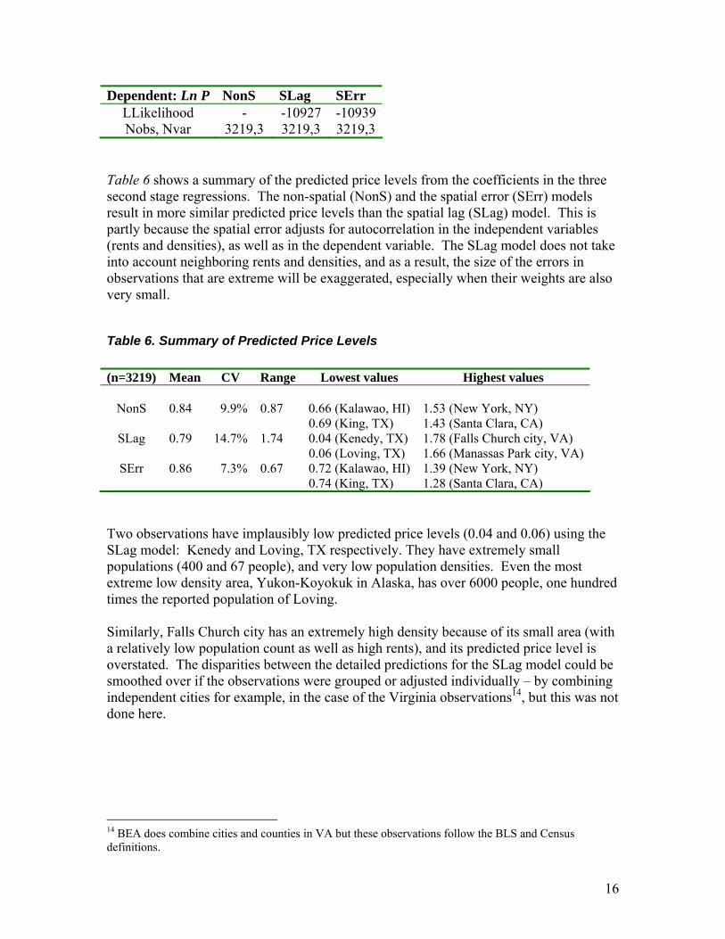
Dependent: Ln P NonS SLag SErr LLikelihood - -10927 -10939Nobs, Nvar 3219,3 3219,3 3219,3

Table 6 shows a summary of the predicted price levels from the coefficients in the three second stage regressions. The non-spatial (NonS) and the spatial error (SErr) models result in more similar predicted price levels than the spatial lag (SLag) model. This is partly because the spatial error adjusts for autocorrelation in the independent variables (rents and densities), as well as in the dependent variable. The SLag model does not take into account neighboring rents and densities, and as a result, the size of the errors in observations that are extreme will be exaggerated, especially when their weights are also very small.

Table 6. Summary of Predicted Price Levels (n=3219) Mean CV Range Lowest values Highest values

NonS 0.84 9.9% 0.87 0.66 (Kalawao, HI)

0.69 (King, TX) 1.53 (New York, NY) 1.43 (Santa Clara, CA)

SLag 0.79 14.7% 1.74 0.04 (Kenedy, TX) 0.06 (Loving, TX)

1.78 (Falls Church city, VA) 1.66 (Manassas Park city, VA)

SErr 0.86 7.3% 0.67 0.72 (Kalawao, HI) 0.74 (King, TX)

1.39 (New York, NY) 1.28 (Santa Clara, CA)

Two observations have implausibly low predicted price levels (0.04 and 0.06) using the SLag model: Kenedy and Loving, TX respectively. They have extremely small populations (400 and 67 people), and very low population densities. Even the most extreme low density area, Yukon-Koyokuk in Alaska, has over 6000 people, one hundred times the reported population of Loving. Similarly, Falls Church city has an extremely high density because of its small area (with a relatively low population count as well as high rents), and its predicted price level is overstated. The disparities between the detailed predictions for the SLag model could be smoothed over if the observations were grouped or adjusted individually – by combining independent cities for example, in the case of the Virginia observations14, but this was not done here.

14 BEA does combine cities and counties in VA but these observations follow the BLS and Census definitions.

17

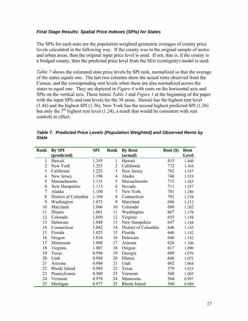
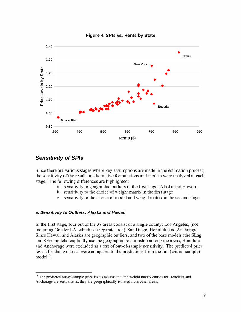
Final Stage Results: Spatial Price Indexes (SPIs) for States The SPIs for each state are the population weighted geometric averages of county price levels calculated in the following way. If the county was in the original sample of metro and urban areas, then the original input price level is used. If not, that is, if the county is a bridged county, then the predicted price level from the SErr (contiguity) model is used. Table 7 shows the estimated state price levels by SPI rank, normalized so that the average of the states equals one. The last two columns show the actual rents observed from the Census, and the corresponding rent levels when these are also normalized across the states to equal one. They are depicted in Figure 4 with rents on the horizontal axis and SPIs on the vertical axis. These mimic Table 1 and Figure 1 at the beginning of the paper with the input SPIs and rent levels for the 38 areas. Hawaii has the highest rent level (1.44) and the highest SPI (1.36). New York has the second highest predicted SPI (1.26) but only the 7th highest rent level (1.24), a result that would be consistent with rent controls in effect.

Table 7. Predicted Price Levels (Population Weighted) and Observed Rents by State Rank By SPI

(predicted) SPI Rank By Rent

(actual) Rent ($) Rent

Level 1 Hawaii 1.355 1 Hawaii 815 1.440 2 New York 1.253 2 California 772 1.364 3 California 1.222 3 New Jersey 762 1.347 4 New Jersey 1.196 4 Alaska 746 1.319 5 Massachusetts 1.151 5 Massachusetts 715 1.263 6 New Hampshire 1.113 6 Nevada 711 1.257 7 Alaska 1.104 7 New York 701 1.240 8 District of Columbia 1.104 8 Connecticut 701 1.238 9 Washington 1.073 9 Maryland 686 1.212

10 Maryland 1.066 10 Colorado 680 1.202 11 Illinois 1.061 11 Washington 667 1.178 12 Colorado 1.050 12 Virginia 655 1.158 13 Delaware 1.048 13 New Hampshire 647 1.144 14 Connecticut 1.042 14 District of Columbia 646 1.142 15 Florida 1.025 15 Florida 646 1.142 16 Oregon 1.016 16 Delaware 646 1.142 17 Minnesota 1.008 17 Arizona 626 1.106 18 Virginia 1.007 18 Oregon 617 1.090 19 Texas 0.994 19 Georgia 609 1.076 20 Utah 0.988 20 Illinois 606 1.072 21 Arizona 0.984 21 Utah 602 1.064 22 Rhode Island 0.984 22 Texas 579 1.023 23 Pennsylvania 0.980 23 Vermont 568 1.005 24 Vermont 0.978 24 Minnesota 564 0.997 25 Michigan 0.977 25 Rhode Island 560 0.989

18

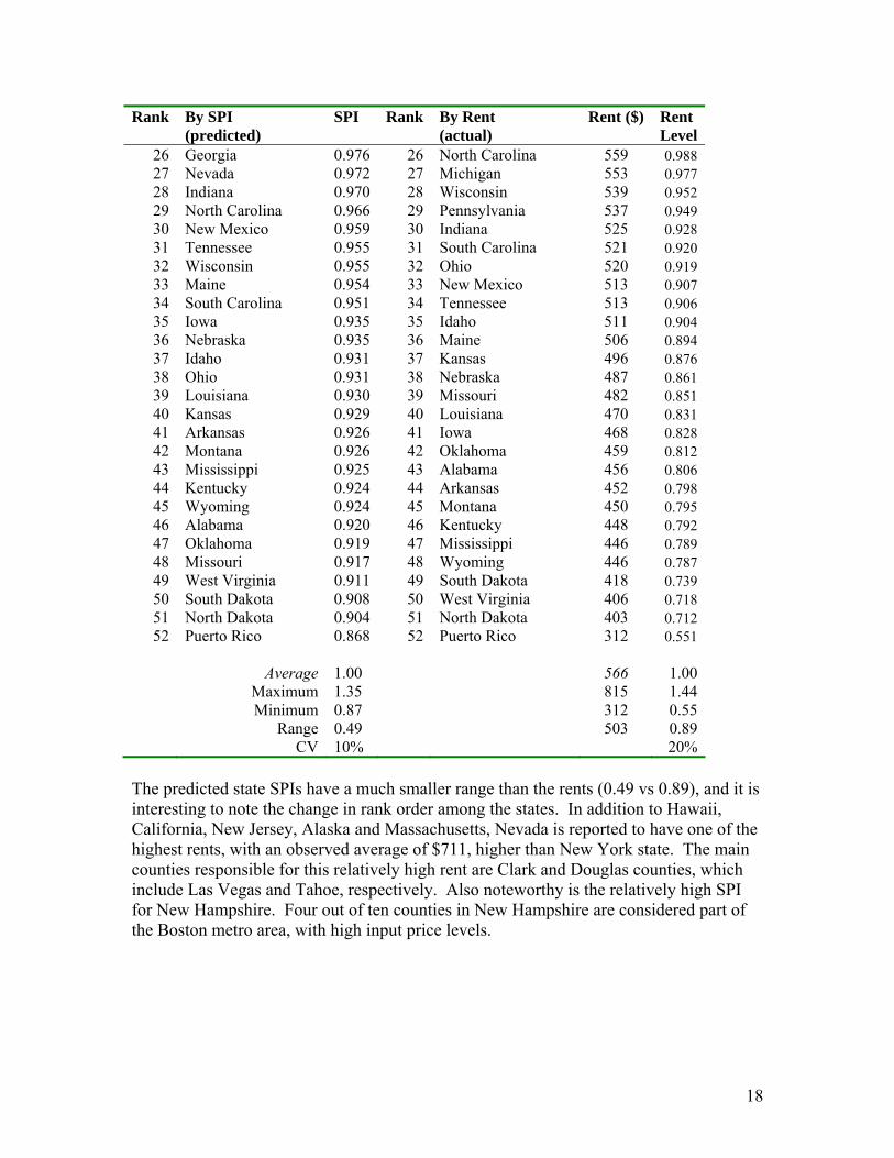
Rank By SPI (predicted)

SPI Rank By Rent (actual)

Rent ($) Rent Level

26 Georgia 0.976 26 North Carolina 559 0.988 27 Nevada 0.972 27 Michigan 553 0.977 28 Indiana 0.970 28 Wisconsin 539 0.952 29 North Carolina 0.966 29 Pennsylvania 537 0.949 30 New Mexico 0.959 30 Indiana 525 0.928 31 Tennessee 0.955 31 South Carolina 521 0.920 32 Wisconsin 0.955 32 Ohio 520 0.919 33 Maine 0.954 33 New Mexico 513 0.907 34 South Carolina 0.951 34 Tennessee 513 0.906 35 Iowa 0.935 35 Idaho 511 0.904 36 Nebraska 0.935 36 Maine 506 0.894 37 Idaho 0.931 37 Kansas 496 0.876 38 Ohio 0.931 38 Nebraska 487 0.861 39 Louisiana 0.930 39 Missouri 482 0.851 40 Kansas 0.929 40 Louisiana 470 0.831 41 Arkansas 0.926 41 Iowa 468 0.828 42 Montana 0.926 42 Oklahoma 459 0.812 43 Mississippi 0.925 43 Alabama 456 0.806 44 Kentucky 0.924 44 Arkansas 452 0.798 45 Wyoming 0.924 45 Montana 450 0.795 46 Alabama 0.920 46 Kentucky 448 0.792 47 Oklahoma 0.919 47 Mississippi 446 0.789 48 Missouri 0.917 48 Wyoming 446 0.787 49 West Virginia 0.911 49 South Dakota 418 0.739 50 South Dakota 0.908 50 West Virginia 406 0.718 51 North Dakota 0.904 51 North Dakota 403 0.712 52 Puerto Rico 0.868 52 Puerto Rico 312 0.551

Average 1.00 566 1.00 Maximum 1.35 815 1.44 Minimum 0.87 312 0.55 Range 0.49 503 0.89 CV 10% 20%

The predicted state SPIs have a much smaller range than the rents (0.49 vs 0.89), and it is interesting to note the change in rank order among the states. In addition to Hawaii, California, New Jersey, Alaska and Massachusetts, Nevada is reported to have one of the highest rents, with an observed average of $711, higher than New York state. The main counties responsible for this relatively high rent are Clark and Douglas counties, which include Las Vegas and Tahoe, respectively. Also noteworthy is the relatively high SPI for New Hampshire. Four out of ten counties in New Hampshire are considered part of the Boston metro area, with high input price levels.

19

Sensitivity of SPIs Since there are various stages where key assumptions are made in the estimation process, the sensitivity of the results to alternative formulations and models were analyzed at each stage. The following differences are highlighted:

a. sensitivity to geographic outliers in the first stage (Alaska and Hawaii) b. sensitivity to the choice of weight matrix in the first stage c. sensitivity to the choice of model and weight matrix in the second stage

a. Sensitivity to Outliers: Alaska and Hawaii In the first stage, four out of the 38 areas consist of a single county: Los Angeles, (not including Greater LA, which is a separate area), San Diego, Honolulu and Anchorage. Since Hawaii and Alaska are geographic outliers, and two of the base models (the SLag and SErr models) explicitly use the geographic relationship among the areas, Honolulu and Anchorage were excluded as a test of out-of-sample sensitivity. The predicted price levels for the two areas were compared to the predictions from the full (within-sample) model15.

15 The predicted out-of-sample price levels assume that the weight matrix entries for Honolulu and Anchorage are zero, that is, they are geographically isolated from other areas.

Figure 4. SPIs vs. Rents by State

0.80

0.90

1.00

1.10

1.20

1.30

1.40

300 400 500 600 700 800 900

Rents ($)

Pric

e Le

vels

by

Stat

e

New York

Nevada

Hawaii

Puerto Rico

20

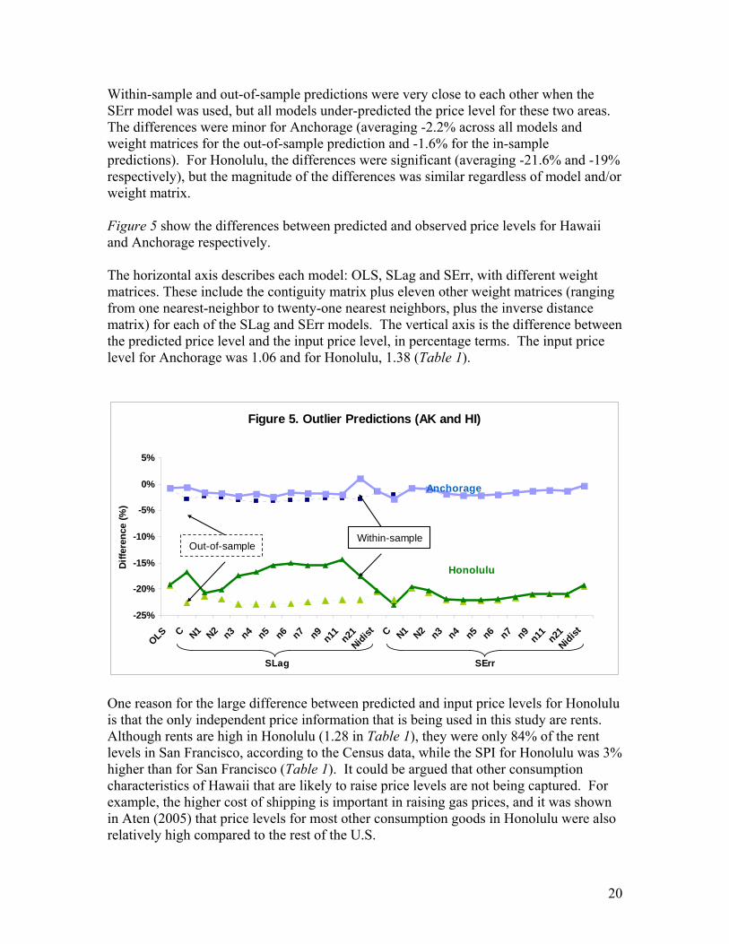
Within-sample and out-of-sample predictions were very close to each other when the SErr model was used, but all models under-predicted the price level for these two areas. The differences were minor for Anchorage (averaging -2.2% across all models and weight matrices for the out-of-sample prediction and -1.6% for the in-sample predictions). For Honolulu, the differences were significant (averaging -21.6% and -19% respectively), but the magnitude of the differences was similar regardless of model and/or weight matrix. Figure 5 show the differences between predicted and observed price levels for Hawaii and Anchorage respectively. The horizontal axis describes each model: OLS, SLag and SErr, with different weight matrices. These include the contiguity matrix plus eleven other weight matrices (ranging from one nearest-neighbor to twenty-one nearest neighbors, plus the inverse distance matrix) for each of the SLag and SErr models. The vertical axis is the difference between the predicted price level and the input price level, in percentage terms. The input price level for Anchorage was 1.06 and for Honolulu, 1.38 (Table 1).

One reason for the large difference between predicted and input price levels for Honolulu is that the only independent price information that is being used in this study are rents. Although rents are high in Honolulu (1.28 in Table 1), they were only 84% of the rent levels in San Francisco, according to the Census data, while the SPI for Honolulu was 3% higher than for San Francisco (Table 1). It could be argued that other consumption characteristics of Hawaii that are likely to raise price levels are not being captured. For example, the higher cost of shipping is important in raising gas prices, and it was shown in Aten (2005) that price levels for most other consumption goods in Honolulu were also relatively high compared to the rest of the U.S.

Figure 5. Outlier Predictions (AK and HI)

-25%

-20%

-15%

-10%

-5%

0%

5%

OLS C N1 N2 n3 n4 n5 n6 n7 n9n11 n21

Nidist C N1 N2 n3 n4 n5 n6 n7 n9n11 n21

Nidist

Diff

eren

ce (%

)

Anchorage

Honolulu

Out-of-sampleWithin-sample

SLag SErr

21

Note that although the model severely under-predicts the price level for Honolulu, the observed price level is the one used for subsequent stages, as there is only one county in Honolulu. This is true for Anchorage and the other two single county areas (Los Angeles and San Diego) as well. For areas with more than one county, the mean of the predicted price level is normalized to the observed price level, so that in effect, we are using only the variation about the mean for the prediction of the within-area counties, not the actual levels.

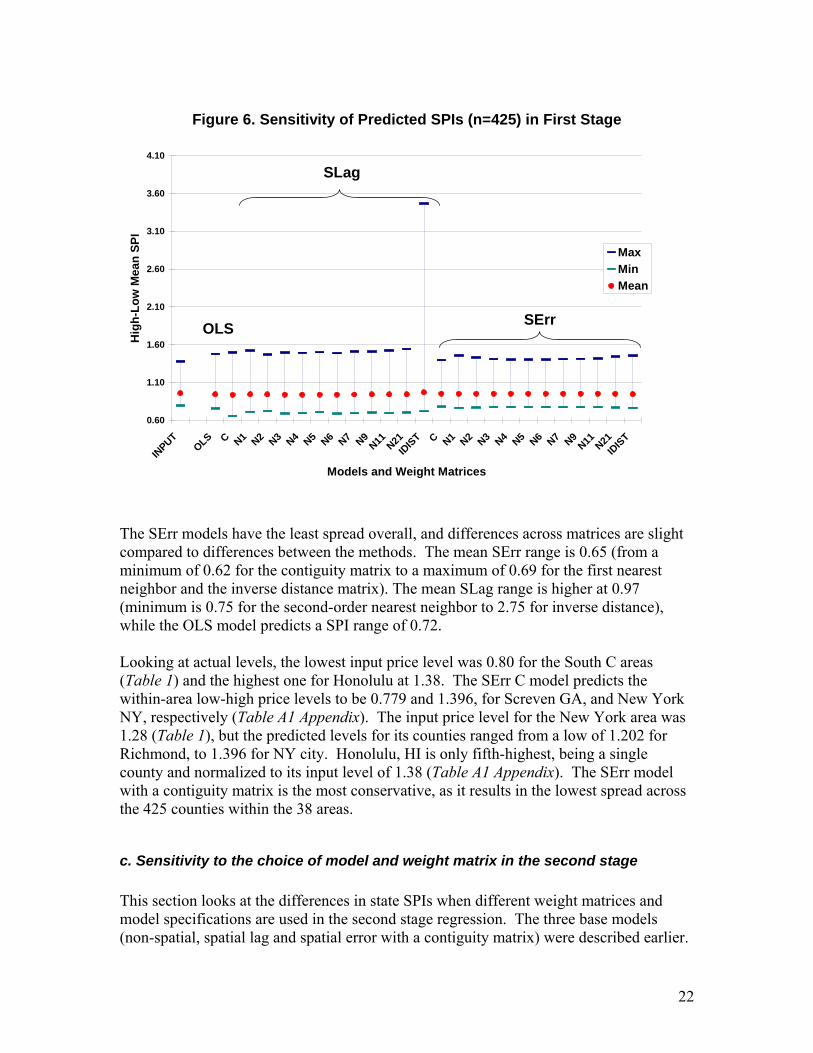
b. Sensitivity to the choice of weight matrix in the first stage The first stage regression results shown in Table 2 used the Contiguity matrix as the spatial weight. Eleven other matrices were created to test the sensitivity of the model to the choice of weights in the SLag and SErr models. These consist of nearest neighbor matrices ranging from first-order nearest neighbor to twenty-first order (one to seven, nine, eleven and twenty-one neighbors), and an inverse distance matrix. The latter resulted in some disproportionately high and low values in the SLag model, partly due to some spatial units that are very close together, as discussed earlier in the text. In the first-order nearest neighbor matrix W, each row has only one entry (equal to 1), corresponding to the nearest observation. For example, W19 = 1 (the 9th observation is the nearest neighbor to the first observation). However, W is not necessarily symmetric, as the nearest neighbor to the 9th observation is observation 8, so W91=0 and W98=1. The second-order nearest neighbor matrix will have two entries per row, each equal to 0.5, while the twenty-first order matrix has 21 entries, each equal to 0.0476. In Figure 6 the different methods are listed on the horizontal axis while the range of the resulting SPIs are on the vertical axis. The range is the maximum predicted county price level minus the minimum predicted county price level for the 425 counties comprising the 38 input areas.

22

The SErr models have the least spread overall, and differences across matrices are slight compared to differences between the methods. The mean SErr range is 0.65 (from a minimum of 0.62 for the contiguity matrix to a maximum of 0.69 for the first nearest neighbor and the inverse distance matrix). The mean SLag range is higher at 0.97 (minimum is 0.75 for the second-order nearest neighbor to 2.75 for inverse distance), while the OLS model predicts a SPI range of 0.72. Looking at actual levels, the lowest input price level was 0.80 for the South C areas (Table 1) and the highest one for Honolulu at 1.38. The SErr C model predicts the within-area low-high price levels to be 0.779 and 1.396, for Screven GA, and New York NY, respectively (Table A1 Appendix). The input price level for the New York area was 1.28 (Table 1), but the predicted levels for its counties ranged from a low of 1.202 for Richmond, to 1.396 for NY city. Honolulu, HI is only fifth-highest, being a single county and normalized to its input level of 1.38 (Table A1 Appendix). The SErr model with a contiguity matrix is the most conservative, as it results in the lowest spread across the 425 counties within the 38 areas.

c. Sensitivity to the choice of model and weight matrix in the second stage This section looks at the differences in state SPIs when different weight matrices and model specifications are used in the second stage regression. The three base models (non-spatial, spatial lag and spatial error with a contiguity matrix) were described earlier.

Figure 6. Sensitivity of Predicted SPIs (n=425) in First Stage

0.60

1.10

1.60

2.10

2.60

3.10

3.60

4.10

INPUT

OLS C N1

N2

N3

N4

N5

N6

N7

N9

N11

N21 ID

IST C N1

N2

N3

N4

N5

N6

N7

N9

N11

N21 ID

IST

Models and Weight Matrices

Hig

h-Lo

w M

ean

SPI

MaxMinMean

SErr

SLag

OLS

23

The spatial lag model gives rise to implausible predicted levels when the values of the independent variables are extreme, combined with very low weights. These differences can be mitigated by joining observations to form different spatial units, but this exercise was not done here. Instead, various weight matrices were created for the full set of 3219 observations, and the resulting state SPIs were compared. Table A3 in the Appendix lists the states in alphabetical order. The Freq column indicates the number of counties within each state. The other columns are the price levels of observed rents (column 1), the input price levels for the first stage regression (column 2), the input price levels for the second stage regression (column 3) and then the various estimated final state SPIs using different methods and matrices. These are the preferred method with the SErr model and contiguity matrix (column 4), the SLag with contiguity (column 5), the NonS model (column 6), followed by columns 7-12 containing the SErr model with a first-order nearest neighbor matrix (n1), a third-order matrix (n3), fifth-order (n5), seventh-order (n7), ninth-order (n9), and eleventh-order (n11) nearest neighbor matrix. Lastly, two more SErr models are shown, one with only regional dummies (column 13), and one with both regional dummies and separate slopes for rents and densities (column 14). Both use the contiguity spatial weight matrix. All levels are normalized to the average of the states for comparison purposes. Hawaii is consistently the highest priced state, followed by New York, California and New Jersey. Puerto Rico is always the lowest, with West Virginia or North Dakota vying for second lowest place. The results are fairly consistent across methods, with the largest differences to be found between the SErr models, regardless of matrix, and the SLag and NonS models (columns 5 & 6). The latter two predict state SPIs that are more similar to those of the SErr models with dummy variables (columns 13 &14). The greatest range was in the SLag model and the NonS model (0.57), while the smallest range (0.49) was in the SErr models, for the contiguity matrix (column 4) and the fifth to eleventh nearest neighbor matrices (columns 9-12). One disadvantage of the unconstrained SErr model with separate slopes and intercepts by region (column 14), is that there are outliers within each region, resulting in predicted SPI for these outliers that are arguably under or over-predictions. For example, states in the Northeast region versus the South. The Northeast region has a higher average and thus Maine’s predicted SPI is 1.01 in column 14, but only 0.95 in all other columns. Conversely, Alabama and Arkansas drop from about 0.92 in the SErr models to 0.89 with a regional dummy for the South, as in column 14. In the first stage, the use of regional dummies was justified because it was a subset of counties that represented only metropolitan and urban areas, and these were scattered across the country. In this second stage, all counties are included and the geographic coverage is over a more continuous surface.

24

Conclusions The state SPIs are constructed from a starting set of 38 metropolitan and urban area price levels for consumption goods and services, plus detailed rent data for all U.S. counties from the 2000 Census. Although the 38 areas in the CPI cover approximately 87% of the U.S. population, geographically they account for only 15% of the counties. The first stage of this exercise breaks down the original 38 areas into 425 counties and estimates price levels that are based on the relationship between rents, population densities and geographic proximity among the observations, and then normalizes them to the original observed BLS means in each area. The second stage involves bridging the estimates for these 425 counties to all other counties, 3219 in total (including the 78 municipalities in Puerto Rico). There is no direct price level information from the BLS for these other counties, as they are not included in the BLS sampling framework of the CPI. However, the Census does have detailed rent data and complete coverage of all counties, and as rents16, on average, account for nearly thirty percent of overall consumer expenditures, they are used as the main auxiliary data in this stage. As first step, we take the rent ratios between sampled and non-sampled areas and apply that ratio to the existing price levels. The assumption is that as a first approximation, the ratio of price levels between the overlap counties (belonging to both BLS and Census samples) and the counties only sampled by the Census is the same as the ratio of their rents. These initial price levels, called bridged price levels, are then regressed against the individual rents and population densities for all 3219 counties. The regression model mirrors the first stage model, and includes a spatial matrix that makes explicit the geographic proximity of the counties, this time with fuller and continuous coverage. The resulting predicted price levels for each non-sampled county are then aggregated to the state level, resulting in a second-round approximation of the state-level spatial price indexes or SPIs. Hawaii had the highest SPI: 35.5% higher than the average of the states, followed by New York and California. Other states that were at least ten percent higher than the average were New Jersey, Massachusetts, New Hampshire, Alaska, and the District of Columbia. States with the lowest price level index were Puerto Rico17 at 86.8% of the average, North and South Dakota and West Virginia, all around the 91% level. Nevada is a state with relatively high rent levels (1.26) but a low SPI (0.97). while New York is the opposite: lower rent level (1.24) but a higher relative SPI (1.25). The range of the SPIs is about 50%, from 15% below average to 35% above average, a much lower range than the rents that vary from a minimum of $312 to a maximum of $815, equivalent to a range of 90%. 16 Rents in the BLS include both Rents and Owner Equivalent Rents (for a more detailed description, see Aten [2006]) 17 As noted earlier, Puerto Rico is not a state but has a full set of sampled rents in the Census, so was included in this study.

25

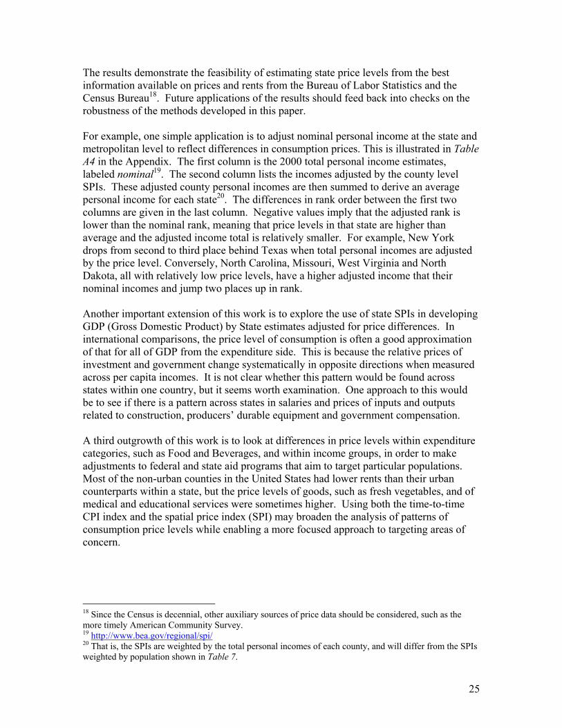
The results demonstrate the feasibility of estimating state price levels from the best information available on prices and rents from the Bureau of Labor Statistics and the Census Bureau18. Future applications of the results should feed back into checks on the robustness of the methods developed in this paper. For example, one simple application is to adjust nominal personal income at the state and metropolitan level to reflect differences in consumption prices. This is illustrated in Table A4 in the Appendix. The first column is the 2000 total personal income estimates, labeled nominal19. The second column lists the incomes adjusted by the county level SPIs. These adjusted county personal incomes are then summed to derive an average personal income for each state20. The differences in rank order between the first two columns are given in the last column. Negative values imply that the adjusted rank is lower than the nominal rank, meaning that price levels in that state are higher than average and the adjusted income total is relatively smaller. For example, New York drops from second to third place behind Texas when total personal incomes are adjusted by the price level. Conversely, North Carolina, Missouri, West Virginia and North Dakota, all with relatively low price levels, have a higher adjusted income that their nominal incomes and jump two places up in rank. Another important extension of this work is to explore the use of state SPIs in developing GDP (Gross Domestic Product) by State estimates adjusted for price differences. In international comparisons, the price level of consumption is often a good approximation of that for all of GDP from the expenditure side. This is because the relative prices of investment and government change systematically in opposite directions when measured across per capita incomes. It is not clear whether this pattern would be found across states within one country, but it seems worth examination. One approach to this would be to see if there is a pattern across states in salaries and prices of inputs and outputs related to construction, producers’ durable equipment and government compensation. A third outgrowth of this work is to look at differences in price levels within expenditure categories, such as Food and Beverages, and within income groups, in order to make adjustments to federal and state aid programs that aim to target particular populations. Most of the non-urban counties in the United States had lower rents than their urban counterparts within a state, but the price levels of goods, such as fresh vegetables, and of medical and educational services were sometimes higher. Using both the time-to-time CPI index and the spatial price index (SPI) may broaden the analysis of patterns of consumption price levels while enabling a more focused approach to targeting areas of concern.

18 Since the Census is decennial, other auxiliary sources of price data should be considered, such as the more timely American Community Survey. 19 http://www.bea.gov/regional/spi/ 20 That is, the SPIs are weighted by the total personal incomes of each county, and will differ from the SPIs weighted by population shown in Table 7.

26

REFERENCES Alegretto, Sylvia http://www.epi.org/content.cfm/bp165 Anselin, Luc (1988), ‘Spatial Econometrics: Methods and Models’, Dordrecht, Kluwer. Anselin, Luc and Julie Le Gallo (2006), ‘Interpolation of Air Quality Measures in Hedonic Price Models: Spatial Aspects’, Spatial Economic Analysis, Vol.1, No.1, June. Anselin, Luc (2002), ‘Under the Hood. Issues in the Specification and Interpretation of Spatial Regression Models’, Anselin, Luc, R.J. Florax & S.J. Rey (2004), ‘Advances in Spatial Econometrics: Methodology, Tools and Applications’, Springer, Berlin. Aten, Bettina (2005), ‘Report on Interarea Price Levels, 2003’, working paper 2005–11, Bureau of Economic Analysis, May. (http://bea.gov/papers/working_papers.htm) Aten, Bettina (2006), ‘Interarea Price Levels: an experimental methodology’, Monthly Labor Review, Vol. 129, No.9, Bureau of Labor Statistics, Washington, DC, September 2006. Ball, Adrian and David Fenwick (2004), ‘ Relative Regional Consumer Price Levels in 2003’, Economic Trends, vol 603, Office for National Statistics, UK. Bernstein, Jared, Chauna Brocht, and Maggie Spade-Aguilar, (2000), ‘How Much Is Enough? Basic Family Budgets for Working Families’, Economic Policy Institute, Washington, D.C.. Fuchs, Victor, Michael Roberts and Sharon Scott (1979), ‘A State Price Index’, National Bureau of Economic Research, Working Paper Series, February. Getis, Art, J.Mure & H.G. Zollerl (2004), ‘Spatial Econometrics and Spatial Statistics’, Londong, Palgrave Macmillan. Goodchild, Michael, Luc Anselin and U. Deichmann (1993), ‘A Framework for the areal interpolation of socioeconomic data’, Environment and Planning A, Vol. 25, Issue 25. Gotway, Carol and Linda Young (2002), ‘ Combining Incompatible Spatial Data’, Journal of the American Statistical Association, June, Vol. 97, No. 458. Holt D., Stell D., Trammer M, Wrighley N. (1996), ‘Aggregation and ecological effects in geographically based data’, in Geographical analysis, Vol. 28, n°. 3. Huang, H.-C. and Cressie, N. (1997), ‘Multiscale spatial modeling’, in 1997 Proceedings of the Section on Statistics and the Environment, 49-54. American Statistical Association, Alexan- dria, VA.

27

Johnson, David S., John M. Rogers, and Lucilla Tan. 2001. "A Century of Family Budgets in the United States." Monthly Labor Review, Vol. 124, No. 5. Bureau of Labor Statistics, Washington, DC. LeSage, J.P. & Pace, R.K. (2004), ‘Advances in Econometrics: Spatial and Spatiotemporal Econometrics’, Elsevier Science, Oxford. Roos, Michael (2006), ‘Regional Price Levels in Germany’, Applied Economics, Vol.38, Issue 13. July.

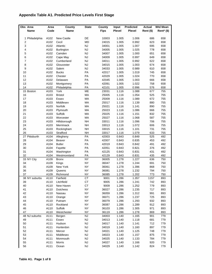
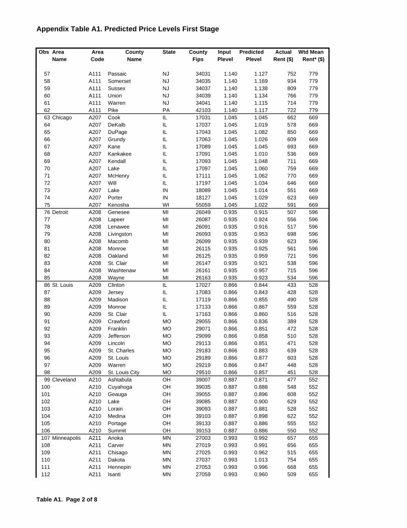
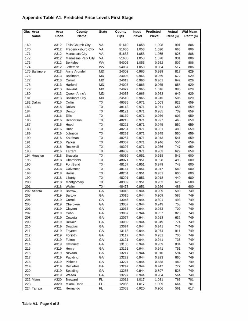
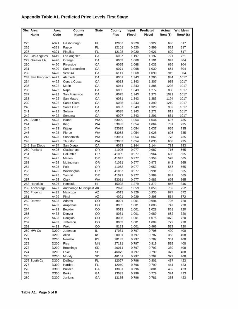
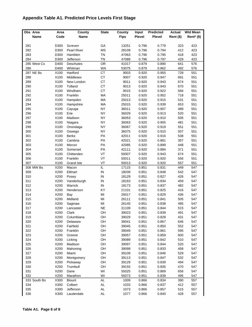
Appendix Table A1. Predicted Price Levels First Stage

Obs Area Area County State County Input Predicted Actual Wtd MeanName Code Name Fips Plevel Plevel Rent ($) Rent* ($)

1 Philadelphia A102 New Castle DE 10003 1.005 1.006 686 6582 A102 Cecil MD 24015 1.005 0.992 623 6583 A102 Atlantic NJ 34001 1.005 1.007 695 6584 A102 Burlington NJ 34005 1.005 1.025 778 6585 A102 Camden NJ 34007 1.005 1.000 651 6586 A102 Cape May NJ 34009 1.005 0.997 649 6587 A102 Cumberland NJ 34011 1.005 0.992 622 6588 A102 Gloucester NJ 34015 1.005 1.003 674 6589 A102 Salem NJ 34033 1.005 0.989 610 658

10 A102 Bucks PA 42017 1.005 1.019 745 65811 A102 Chester PA 42029 1.005 1.024 770 65812 A102 Delaware PA 42045 1.005 1.003 666 65813 A102 Montgomery PA 42091 1.005 1.022 758 65814 A102 Philadelphia PA 42101 1.005 0.996 576 65815 Boston A103 York ME 23031 1.116 1.088 677 75516 A103 Bristol MA 25005 1.116 1.054 525 75517 A103 Essex MA 25009 1.116 1.089 672 75518 A103 Middlesex MA 25017 1.116 1.139 880 75519 A103 Norfolk MA 25021 1.116 1.141 890 75520 A103 Plymouth MA 25023 1.116 1.086 666 75521 A103 Suffolk MA 25025 1.116 1.151 832 75522 A103 Worcester MA 25027 1.116 1.068 587 75523 A103 Hillsborough NH 33011 1.116 1.096 706 75524 A103 Merrimack NH 33013 1.116 1.072 606 75525 A103 Rockingham NH 33015 1.116 1.101 731 75526 A103 Strafford NH 33017 1.116 1.079 633 75527 Pittsburth A104 Allegheny PA 42003 0.843 0.849 525 49228 A104 Beaver PA 42007 0.843 0.835 453 49229 A104 Butler PA 42019 0.843 0.842 491 49230 A104 Fayette PA 42051 0.843 0.821 376 49231 A104 Washington PA 42125 0.843 0.831 431 49232 A104 Westmoreland PA 42129 0.843 0.831 435 49233 NY City A109 Bronx NY 36005 1.278 1.227 636 75034 A109 Kings NY 36047 1.278 1.244 691 75035 A109 New York NY 36061 1.278 1.396 868 75036 A109 Queens NY 36081 1.278 1.232 794 75037 A109 Richmond NY 36085 1.278 1.202 773 75038 NY suburbs A110 Fairfield CT 9001 1.286 1.357 1157 89339 A110 Litchfield CT 9005 1.286 1.241 742 89340 A110 New Haven CT 9009 1.286 1.252 779 89341 A110 Dutchess NY 36027 1.286 1.235 717 89342 A110 Nassau NY 36059 1.286 1.312 991 89343 A110 Orange NY 36071 1.286 1.237 725 89344 A110 Putnam NY 36079 1.286 1.293 932 89345 A110 Rockland NY 36087 1.286 1.289 912 89346 A110 Suffolk NY 36103 1.286 1.305 971 89347 A110 Westchester NY 36119 1.286 1.278 869 89348 NJ suburbs A111 Bergen NJ 34003 1.140 1.165 901 77949 A111 Essex NJ 34013 1.140 1.118 681 77950 A111 Hudson NJ 34017 1.140 1.141 712 77951 A111 Hunterdon NJ 34019 1.140 1.160 897 77952 A111 Mercer NJ 34021 1.140 1.125 748 77953 A111 Middlesex NJ 34023 1.140 1.157 875 77954 A111 Monmouth NJ 34025 1.140 1.133 784 77955 A111 Morris NJ 34027 1.140 1.166 920 77956 A111 Ocean NJ 34029 1.140 1.142 824 779

Table A1. Page 1 of 8

Appendix Table A1. Predicted Price Levels First Stage

Obs Area Area County State County Input Predicted Actual Wtd MeanName Code Name Fips Plevel Plevel Rent ($) Rent* ($)

57 A111 Passaic NJ 34031 1.140 1.127 752 77958 A111 Somerset NJ 34035 1.140 1.169 934 77959 A111 Sussex NJ 34037 1.140 1.138 809 77960 A111 Union NJ 34039 1.140 1.134 766 77961 A111 Warren NJ 34041 1.140 1.115 714 77962 A111 Pike PA 42103 1.140 1.117 722 77963 Chicago A207 Cook IL 17031 1.045 1.045 662 66964 A207 DeKalb IL 17037 1.045 1.019 578 66965 A207 DuPage IL 17043 1.045 1.082 850 66966 A207 Grundy IL 17063 1.045 1.026 609 66967 A207 Kane IL 17089 1.045 1.045 693 66968 A207 Kankakee IL 17091 1.045 1.010 536 66969 A207 Kendall IL 17093 1.045 1.048 711 66970 A207 Lake IL 17097 1.045 1.060 759 66971 A207 McHenry IL 17111 1.045 1.062 770 66972 A207 Will IL 17197 1.045 1.034 646 66973 A207 Lake IN 18089 1.045 1.014 551 66974 A207 Porter IN 18127 1.045 1.029 623 66975 A207 Kenosha WI 55059 1.045 1.022 591 66976 Detroit A208 Genesee MI 26049 0.935 0.915 507 59677 A208 Lapeer MI 26087 0.935 0.924 556 59678 A208 Lenawee MI 26091 0.935 0.916 517 59679 A208 Livingston MI 26093 0.935 0.953 698 59680 A208 Macomb MI 26099 0.935 0.939 623 59681 A208 Monroe MI 26115 0.935 0.925 561 59682 A208 Oakland MI 26125 0.935 0.959 721 59683 A208 St. Clair MI 26147 0.935 0.921 538 59684 A208 Washtenaw MI 26161 0.935 0.957 715 59685 A208 Wayne MI 26163 0.935 0.923 534 59686 St. Louis A209 Clinton IL 17027 0.866 0.844 433 52887 A209 Jersey IL 17083 0.866 0.843 428 52888 A209 Madison IL 17119 0.866 0.855 490 52889 A209 Monroe IL 17133 0.866 0.867 559 52890 A209 St. Clair IL 17163 0.866 0.860 516 52891 A209 Crawford MO 29055 0.866 0.836 389 52892 A209 Franklin MO 29071 0.866 0.851 472 52893 A209 Jefferson MO 29099 0.866 0.858 510 52894 A209 Lincoln MO 29113 0.866 0.851 471 52895 A209 St. Charles MO 29183 0.866 0.883 639 52896 A209 St. Louis MO 29189 0.866 0.877 603 52897 A209 Warren MO 29219 0.866 0.847 448 52898 A209 St. Louis City MO 29510 0.866 0.857 451 52899 Cleveland A210 Ashtabula OH 39007 0.887 0.871 477 552

100 A210 Cuyahoga OH 39035 0.887 0.888 548 552101 A210 Geauga OH 39055 0.887 0.896 608 552102 A210 Lake OH 39085 0.887 0.900 629 552103 A210 Lorain OH 39093 0.887 0.881 528 552104 A210 Medina OH 39103 0.887 0.898 622 552105 A210 Portage OH 39133 0.887 0.886 555 552106 A210 Summit OH 39153 0.887 0.886 550 552107 Minneapolis A211 Anoka MN 27003 0.993 0.992 657 655108 A211 Carver MN 27019 0.993 0.991 656 655109 A211 Chisago MN 27025 0.993 0.962 515 655110 A211 Dakota MN 27037 0.993 1.013 754 655111 A211 Hennepin MN 27053 0.993 0.996 668 655112 A211 Isanti MN 27059 0.993 0.960 509 655

Table A1. Page 2 of 8

Appendix Table A1. Predicted Price Levels First Stage

Obs Area Area County State County Input Predicted Actual Wtd MeanName Code Name Fips Plevel Plevel Rent ($) Rent* ($)

113 A211 Ramsey MN 27123 0.993 0.986 615 655114 A211 Scott MN 27139 0.993 0.994 667 655115 A211 Sherburne MN 27141 0.993 0.973 568 655116 A211 Washington MN 27163 0.993 1.001 701 655117 A211 Wright MN 27171 0.993 0.963 521 655118 A211 Pierce WI 55093 0.993 0.966 538 655119 A211 St. Croix WI 55109 0.993 0.973 571 655120 Milwaukee A212 Milwaukee WI 55079 0.908 0.904 555 578121 A212 Ozaukee WI 55089 0.908 0.918 651 578122 A212 Racine WI 55101 0.908 0.898 548 578123 A212 Washington WI 55131 0.908 0.913 627 578124 A212 Waukesha WI 55133 0.908 0.931 718 578125 Cincinnati A213 Dearborn IN 18029 0.874 0.870 509 521126 A213 Ohio IN 18115 0.874 0.863 469 521127 A213 Boone KY 21015 0.874 0.889 607 521128 A213 Campbell KY 21037 0.874 0.872 515 521129 A213 Gallatin KY 21077 0.874 0.853 416 521130 A213 Grant KY 21081 0.874 0.871 516 521131 A213 Kenton KY 21117 0.874 0.873 520 521132 A213 Pendleton KY 21191 0.874 0.853 416 521133 A213 Brown OH 39015 0.874 0.858 442 521134 A213 Butler OH 39017 0.874 0.882 567 521135 A213 Clermont OH 39025 0.874 0.880 558 521136 A213 Hamilton OH 39061 0.874 0.871 498 521137 A213 Warren OH 39165 0.874 0.888 605 521138 Kansas City A214 Johnson KS 20091 0.860 0.885 716 576139 A214 Leavenworth KS 20103 0.860 0.857 567 576140 A214 Miami KS 20121 0.860 0.842 484 576141 A214 Wyandotte KS 20209 0.860 0.845 496 576142 A214 Cass MO 29037 0.860 0.847 515 576143 A214 Clay MO 29047 0.860 0.861 589 576144 A214 Clinton MO 29049 0.860 0.833 434 576145 A214 Jackson MO 29095 0.860 0.853 538 576146 A214 Lafayette MO 29107 0.860 0.829 416 576147 A214 Platte MO 29165 0.860 0.873 652 576148 A214 Ray MO 29177 0.860 0.834 443 576149 DC A312 District of Columbia DC 11001 1.058 1.031 646 806150 A312 Calvert MD 24009 1.058 1.046 804 806151 A312 Charles MD 24017 1.058 1.054 838 806152 A312 Frederick MD 24021 1.058 1.032 740 806153 A312 Montgomery MD 24031 1.058 1.078 934 806154 A312 Prince George's MD 24033 1.058 1.037 756 806155 A312 Washington MD 24043 1.058 0.978 489 806156 A312 Arlington VA 51013 1.058 1.098 946 806157 A312 Clarke VA 51043 1.058 1.006 620 806158 A312 Culpeper VA 51047 1.058 0.998 586 806159 A312 Fairfax VA 51059 1.058 1.100 1027 806160 A312 Fauquier VA 51061 1.058 1.034 748 806161 A312 King George VA 51099 1.058 1.008 631 806162 A312 Loudoun VA 51107 1.058 1.088 988 806163 A312 Prince William VA 51153 1.058 1.060 863 806164 A312 Spotsylvania VA 51177 1.058 1.049 815 806165 A312 Stafford VA 51179 1.058 1.059 861 806166 A312 Warren VA 51187 1.058 0.988 539 806167 A312 Alexandria City VA 51510 1.058 1.089 880 806168 A312 Fairfax City VA 51600 1.058 1.090 976 806

Table A1. Page 3 of 8

Appendix Table A1. Predicted Price Levels First Stage

Obs Area Area County State County Input Predicted Actual Wtd MeanName Code Name Fips Plevel Plevel Rent ($) Rent* ($)

169 A312 Falls Church City VA 51610 1.058 1.098 991 806170 A312 Fredericksburg City VA 51630 1.058 1.020 663 806171 A312 Manassas City VA 51683 1.058 1.055 826 806172 A312 Manassas Park City VA 51685 1.058 1.078 931 806173 A312 Berkeley WV 54003 1.058 0.982 507 806174 A312 Jefferson WV 54037 1.058 0.984 517 806175 Baltimore A313 Anne Arundel MD 24003 0.966 0.999 817 629176 A313 Baltimore MD 24005 0.966 0.969 672 629177 A313 Carroll MD 24013 0.966 0.961 642 629178 A313 Harford MD 24025 0.966 0.965 658 629179 A313 Howard MD 24027 0.966 1.016 895 629180 A313 Queen Anne's MD 24035 0.966 0.963 649 629181 A313 Baltimore City MD 24510 0.966 0.945 506 629182 Dallas A316 Collin TX 48085 0.971 1.003 823 659183 A316 Dallas TX 48113 0.971 0.971 656 659184 A316 Denton TX 48121 0.971 0.985 739 659185 A316 Ellis TX 48139 0.971 0.956 603 659186 A316 Henderson TX 48213 0.971 0.927 463 659187 A316 Hood TX 48221 0.971 0.945 552 659188 A316 Hunt TX 48231 0.971 0.931 480 659189 A316 Johnson TX 48251 0.971 0.945 550 659190 A316 Kaufman TX 48257 0.971 0.943 541 659191 A316 Parker TX 48367 0.971 0.946 554 659192 A316 Rockwall TX 48397 0.971 0.986 747 659193 A316 Tarrant TX 48439 0.971 0.963 629 659194 Houston A318 Brazoria TX 48039 0.951 0.938 546 600195 A318 Chambers TX 48071 0.951 0.928 498 600196 A318 Fort Bend TX 48157 0.951 0.979 748 600197 A318 Galveston TX 48167 0.951 0.947 589 600198 A318 Harris TX 48201 0.951 0.951 600 600199 A318 Liberty TX 48291 0.951 0.918 449 600200 A318 Montgomery TX 48339 0.951 0.953 623 600201 A318 Waller TX 48473 0.951 0.926 488 600202 Atlanta A319 Barrow GA 13013 0.944 0.909 590 749203 A319 Bartow GA 13015 0.944 0.909 588 749204 A319 Carroll GA 13045 0.944 0.891 498 749205 A319 Cherokee GA 13057 0.944 0.943 758 749206 A319 Clayton GA 13063 0.944 0.933 700 749207 A319 Cobb GA 13067 0.944 0.957 820 749208 A319 Coweta GA 13077 0.944 0.918 636 749209 A319 DeKalb GA 13089 0.944 0.949 774 749210 A319 Douglas GA 13097 0.944 0.941 748 749211 A319 Fayette GA 13113 0.944 0.974 911 749212 A319 Forsyth GA 13117 0.944 0.931 700 749213 A319 Fulton GA 13121 0.944 0.941 736 749214 A319 Gwinnett GA 13135 0.944 0.959 834 749215 A319 Henry GA 13151 0.944 0.941 751 749216 A319 Newton GA 13217 0.944 0.910 594 749217 A319 Paulding GA 13223 0.944 0.923 660 749218 A319 Pickens GA 13227 0.944 0.888 480 749219 A319 Rockdale GA 13247 0.944 0.947 777 749220 A319 Spalding GA 13255 0.944 0.897 528 749221 A319 Walton GA 13297 0.944 0.904 564 749222 Miami A320 Broward FL 12011 1.017 1.031 765 701223 A320 Miami-Dade FL 12086 1.017 1.009 664 701224 Tampa A321 Hernando FL 12053 0.920 0.906 561 617

Table A1. Page 4 of 8

Appendix Table A1. Predicted Price Levels First Stage

Obs Area Area County State County Input Predicted Actual Wtd MeanName Code Name Fips Plevel Plevel Rent ($) Rent* ($)

225 A321 Hillsborough FL 12057 0.920 0.922 636 617226 A321 Pasco FL 12101 0.920 0.899 522 617227 A321 Pinellas FL 12103 0.920 0.921 620 617228 Los Angeles A419 Los Angeles CA 6037 1.197 1.197 721 721229 Greater LA A420 Orange CA 6059 1.068 1.101 947 804230 A420 Riverside CA 6065 1.068 1.033 669 804231 A420 San Bernardino CA 6071 1.068 1.030 654 804232 A420 Ventura CA 6111 1.068 1.090 919 804233 San Francisco A422 Alameda CA 6001 1.343 1.295 884 1017234 A422 Contra Costa CA 6013 1.343 1.307 935 1017235 A422 Marin CA 6041 1.343 1.386 1208 1017236 A422 Napa CA 6055 1.343 1.277 830 1017237 A422 San Francisco CA 6075 1.343 1.378 1021 1017238 A422 San Mateo CA 6081 1.343 1.383 1194 1017239 A422 Santa Clara CA 6085 1.343 1.390 1219 1017240 A422 Santa Cruz CA 6087 1.343 1.320 982 1017241 A422 Solano CA 6095 1.343 1.272 811 1017242 A422 Sonoma CA 6097 1.343 1.291 881 1017243 Seattle A423 Island WA 53029 1.054 1.044 697 735244 A423 King WA 53033 1.054 1.064 781 735245 A423 Kitsap WA 53035 1.054 1.037 665 735246 A423 Pierce WA 53053 1.054 1.028 626 735247 A423 Snohomish WA 53061 1.054 1.062 778 735248 A423 Thurston WA 53067 1.054 1.035 658 735249 San Diego A424 San Diego CA 6073 1.144 1.144 783 783250 Portland A425 Clackamas OR 41005 0.977 0.987 716 665251 A425 Columbia OR 41009 0.977 0.964 608 665252 A425 Marion OR 41047 0.977 0.958 578 665253 A425 Multnomah OR 41051 0.977 0.973 642 665254 A425 Polk OR 41053 0.977 0.953 557 665255 A425 Washington OR 41067 0.977 0.991 732 665256 A425 Yamhill OR 41071 0.977 0.969 631 665257 A425 Clark WA 53011 0.977 0.983 695 665258 Honolulu A426 Honolulu HI 15003 1.379 1.379 846 846259 Anchorage A427 Anchorage MunicipalityAK 2020 1.059 1.059 752 752260 Phoenix A429 Maricopa AZ 4013 0.929 0.930 677 672261 A429 Pinal AZ 4021 0.929 0.898 514 672262 Denver A433 Adams CO 8001 1.001 0.994 706 720263 A433 Arapahoe CO 8005 1.001 1.003 747 720264 A433 Boulder CO 8013 1.001 1.028 861 720265 A433 Denver CO 8031 1.001 0.989 652 720266 A433 Douglas CO 8035 1.001 1.075 1072 720267 A433 Jefferson CO 8059 1.001 1.009 772 720268 A433 Weld CO 8123 1.001 0.966 572 720269 MW Cs D200 Jefferson IL 17081 0.797 0.795 400 408270 D200 Allen KS 20001 0.797 0.787 353 408271 D200 Neosho KS 20133 0.797 0.787 351 408272 D200 Rice MN 27131 0.797 0.815 515 408273 D200 Brookings SD 46011 0.797 0.793 389 408274 D200 Lake SD 46079 0.797 0.790 372 408275 D200 Moody SD 46101 0.797 0.792 379 408276 South Cs D300 DeSoto FL 12027 0.796 0.801 457 423277 D300 Hardee FL 12049 0.796 0.799 444 423278 D300 Bulloch GA 13031 0.796 0.801 452 423279 D300 Burke GA 13033 0.796 0.779 324 423280 D300 Jenkins GA 13165 0.796 0.781 335 423

Table A1. Page 5 of 8

Appendix Table A1. Predicted Price Levels First Stage

Obs Area Area County State County Input Predicted Actual Wtd MeanName Code Name Fips Plevel Plevel Rent ($) Rent* ($)

281 D300 Screven GA 13251 0.796 0.779 323 423282 D300 Pearl River MS 28109 0.796 0.794 412 423283 D300 Hamblen TN 47063 0.796 0.795 418 423284 D300 Jefferson TN 47089 0.796 0.797 429 423285 West Cs D400 Deschutes OR 41017 0.879 0.890 641 576286 D400 Whitman WA 53075 0.879 0.862 492 576287 NE Bs X100 Hartford CT 9003 0.920 0.955 728 551288 X100 Middlesex CT 9007 0.920 0.947 691 551289 X100 New London CT 9011 0.920 0.943 674 551290 X100 Tolland CT 9013 0.920 0.943 670 551291 X100 Windham CT 9015 0.920 0.922 566 551292 X100 Franklin MA 25011 0.920 0.952 718 551293 X100 Hampden MA 25013 0.920 0.915 531 551294 X100 Hampshire MA 25015 0.920 0.939 653 551295 X100 Cayuga NY 36011 0.920 0.907 489 551296 X100 Erie NY 36029 0.920 0.913 520 551297 X100 Madison NY 36053 0.920 0.910 505 551298 X100 Niagara NY 36063 0.920 0.905 481 551299 X100 Onondaga NY 36067 0.920 0.919 551 551300 X100 Oswego NY 36075 0.920 0.910 507 551301 X100 Berks PA 42011 0.920 0.916 538 551302 X100 Cambria PA 42021 0.920 0.881 357 551303 X100 Mercer PA 42085 0.920 0.899 448 551304 X100 Somerset PA 42111 0.920 0.884 371 551305 X100 Chittenden VT 50007 0.920 0.943 674 551306 X100 Franklin VT 50011 0.920 0.920 556 551307 X100 Grand Isle VT 50013 0.920 0.920 557 551308 MW Bs X200 Macon IL 17115 0.851 0.831 449 547309 X200 Elkhart IN 18039 0.851 0.848 542 547310 X200 Posey IN 18129 0.851 0.827 426 547311 X200 Vanderburgh IN 18163 0.851 0.834 459 547312 X200 Warrick IN 18173 0.851 0.837 482 547313 X200 Henderson KY 21101 0.851 0.825 416 547314 X200 Bay MI 26017 0.851 0.829 436 547315 X200 Midland MI 26111 0.851 0.841 505 547316 X200 Saginaw MI 26145 0.851 0.838 485 547317 X200 Lancaster NE 31109 0.851 0.844 515 547318 X200 Clark OH 39023 0.851 0.839 491 547319 X200 Columbiana OH 39029 0.851 0.828 431 547320 X200 Delaware OH 39041 0.851 0.867 646 547321 X200 Fairfield OH 39045 0.851 0.850 552 547322 X200 Franklin OH 39049 0.851 0.861 595 547323 X200 Greene OH 39057 0.851 0.859 600 547324 X200 Licking OH 39089 0.851 0.842 510 547325 X200 Madison OH 39097 0.851 0.844 520 547326 X200 Mahoning OH 39099 0.851 0.833 458 547327 X200 Miami OH 39109 0.851 0.846 529 547328 X200 Montgomery OH 39113 0.851 0.847 532 547329 X200 Pickaway OH 39129 0.851 0.839 494 547330 X200 Trumbull OH 39155 0.851 0.835 470 547331 X200 Dane WI 55025 0.851 0.869 656 547332 X200 Marathon WI 55073 0.851 0.839 495 547333 South Bs X300 Blount AL 1009 0.866 0.834 390 557334 X300 Colbert AL 1033 0.866 0.837 412 557335 X300 Jefferson AL 1073 0.866 0.857 515 557336 X300 Lauderdale AL 1077 0.866 0.840 428 557

Table A1. Page 6 of 8

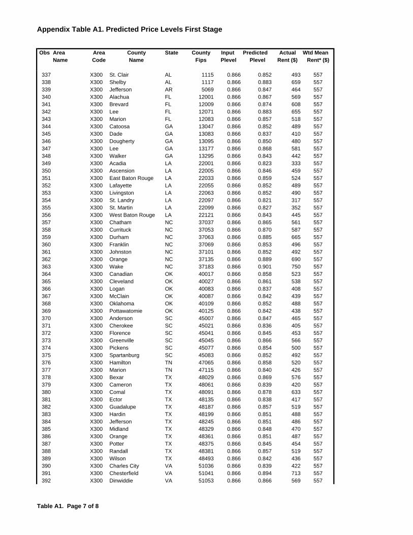
Appendix Table A1. Predicted Price Levels First Stage

Obs Area Area County State County Input Predicted Actual Wtd MeanName Code Name Fips Plevel Plevel Rent ($) Rent* ($)

337 X300 St. Clair AL 1115 0.866 0.852 493 557338 X300 Shelby AL 1117 0.866 0.883 659 557339 X300 Jefferson AR 5069 0.866 0.847 464 557340 X300 Alachua FL 12001 0.866 0.867 569 557341 X300 Brevard FL 12009 0.866 0.874 608 557342 X300 Lee FL 12071 0.866 0.883 655 557343 X300 Marion FL 12083 0.866 0.857 518 557344 X300 Catoosa GA 13047 0.866 0.852 489 557345 X300 Dade GA 13083 0.866 0.837 410 557346 X300 Dougherty GA 13095 0.866 0.850 480 557347 X300 Lee GA 13177 0.866 0.868 581 557348 X300 Walker GA 13295 0.866 0.843 442 557349 X300 Acadia LA 22001 0.866 0.823 333 557350 X300 Ascension LA 22005 0.866 0.846 459 557351 X300 East Baton Rouge LA 22033 0.866 0.859 524 557352 X300 Lafayette LA 22055 0.866 0.852 489 557353 X300 Livingston LA 22063 0.866 0.852 490 557354 X300 St. Landry LA 22097 0.866 0.821 317 557355 X300 St. Martin LA 22099 0.866 0.827 352 557356 X300 West Baton Rouge LA 22121 0.866 0.843 445 557357 X300 Chatham NC 37037 0.866 0.865 561 557358 X300 Currituck NC 37053 0.866 0.870 587 557359 X300 Durham NC 37063 0.866 0.885 665 557360 X300 Franklin NC 37069 0.866 0.853 496 557361 X300 Johnston NC 37101 0.866 0.852 492 557362 X300 Orange NC 37135 0.866 0.889 690 557363 X300 Wake NC 37183 0.866 0.901 750 557364 X300 Canadian OK 40017 0.866 0.858 523 557365 X300 Cleveland OK 40027 0.866 0.861 538 557366 X300 Logan OK 40083 0.866 0.837 408 557367 X300 McClain OK 40087 0.866 0.842 439 557368 X300 Oklahoma OK 40109 0.866 0.852 488 557369 X300 Pottawatomie OK 40125 0.866 0.842 438 557370 X300 Anderson SC 45007 0.866 0.847 465 557371 X300 Cherokee SC 45021 0.866 0.836 405 557372 X300 Florence SC 45041 0.866 0.845 453 557373 X300 Greenville SC 45045 0.866 0.866 566 557374 X300 Pickens SC 45077 0.866 0.854 500 557375 X300 Spartanburg SC 45083 0.866 0.852 492 557376 X300 Hamilton TN 47065 0.866 0.858 520 557377 X300 Marion TN 47115 0.866 0.840 426 557378 X300 Bexar TX 48029 0.866 0.869 576 557379 X300 Cameron TX 48061 0.866 0.839 420 557380 X300 Comal TX 48091 0.866 0.878 633 557381 X300 Ector TX 48135 0.866 0.838 417 557382 X300 Guadalupe TX 48187 0.866 0.857 519 557383 X300 Hardin TX 48199 0.866 0.851 488 557384 X300 Jefferson TX 48245 0.866 0.851 486 557385 X300 Midland TX 48329 0.866 0.848 470 557386 X300 Orange TX 48361 0.866 0.851 487 557387 X300 Potter TX 48375 0.866 0.845 454 557388 X300 Randall TX 48381 0.866 0.857 519 557389 X300 Wilson TX 48493 0.866 0.842 436 557390 X300 Charles City VA 51036 0.866 0.839 422 557391 X300 Chesterfield VA 51041 0.866 0.894 713 557392 X300 Dinwiddie VA 51053 0.866 0.866 569 557

Table A1. Page 7 of 8

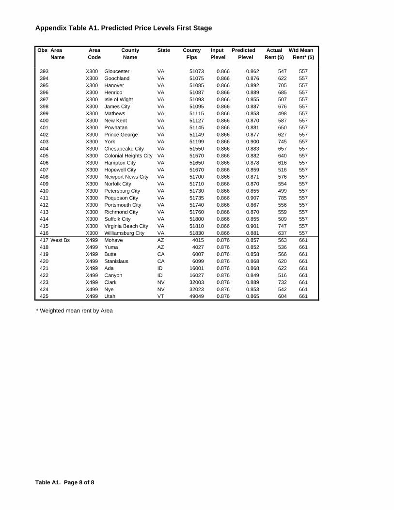
Appendix Table A1. Predicted Price Levels First Stage

Obs Area Area County State County Input Predicted Actual Wtd MeanName Code Name Fips Plevel Plevel Rent ($) Rent* ($)

393 X300 Gloucester VA 51073 0.866 0.862 547 557394 X300 Goochland VA 51075 0.866 0.876 622 557395 X300 Hanover VA 51085 0.866 0.892 705 557396 X300 Henrico VA 51087 0.866 0.889 685 557397 X300 Isle of Wight VA 51093 0.866 0.855 507 557398 X300 James City VA 51095 0.866 0.887 676 557399 X300 Mathews VA 51115 0.866 0.853 498 557400 X300 New Kent VA 51127 0.866 0.870 587 557401 X300 Powhatan VA 51145 0.866 0.881 650 557402 X300 Prince George VA 51149 0.866 0.877 627 557403 X300 York VA 51199 0.866 0.900 745 557404 X300 Chesapeake City VA 51550 0.866 0.883 657 557405 X300 Colonial Heights City VA 51570 0.866 0.882 640 557406 X300 Hampton City VA 51650 0.866 0.878 616 557407 X300 Hopewell City VA 51670 0.866 0.859 516 557408 X300 Newport News City VA 51700 0.866 0.871 576 557409 X300 Norfolk City VA 51710 0.866 0.870 554 557410 X300 Petersburg City VA 51730 0.866 0.855 499 557411 X300 Poquoson City VA 51735 0.866 0.907 785 557412 X300 Portsmouth City VA 51740 0.866 0.867 556 557413 X300 Richmond City VA 51760 0.866 0.870 559 557414 X300 Suffolk City VA 51800 0.866 0.855 509 557415 X300 Virginia Beach City VA 51810 0.866 0.901 747 557416 X300 Williamsburg City VA 51830 0.866 0.881 637 557417 West Bs X499 Mohave AZ 4015 0.876 0.857 563 661418 X499 Yuma AZ 4027 0.876 0.852 536 661419 X499 Butte CA 6007 0.876 0.858 566 661420 X499 Stanislaus CA 6099 0.876 0.868 620 661421 X499 Ada ID 16001 0.876 0.868 622 661422 X499 Canyon ID 16027 0.876 0.849 516 661423 X499 Clark NV 32003 0.876 0.889 732 661424 X499 Nye NV 32023 0.876 0.853 542 661425 X499 Utah VT 49049 0.876 0.865 604 661

* Weighted mean rent by Area

Table A1. Page 8 of 8

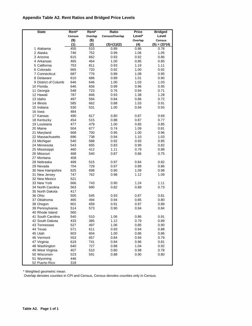
Appendix Table A2. Rent Ratios and Bridged Price Levels

State Rent* Rent* Ratio Price Bridged Census Overlap Census/Overlap Level* Level

($) ($) Overlap Census(1) (2) (3)=(1)/(2) (4) (5) = (3)*(4)

1 Alabama 455 510 0.89 0.86 0.762 Alaska 746 752 0.99 1.06 1.053 Arizona 615 662 0.93 0.92 0.864 Arkansas 465 464 1.00 0.85 0.855 California 753 811 0.93 1.19 1.116 Colorado 665 720 0.92 1.00 0.927 Connecticut 687 776 0.89 1.08 0.958 Delaware 610 686 0.89 1.01 0.909 District of Columb 646 646 1.00 1.03 1.03

10 Florida 646 656 0.99 0.96 0.9511 Georgia 548 723 0.76 0.94 0.7112 Hawaii 787 846 0.93 1.38 1.2813 Idaho 497 594 0.84 0.86 0.7214 Illinois 585 662 0.88 1.03 0.9115 Indiana 530 531 1.00 0.94 0.9316 Iowa 48417 Kansas 490 617 0.80 0.87 0.6918 Kentucky 454 515 0.88 0.87 0.7719 Louisiana 477 479 1.00 0.85 0.8520 Maine 504 677 0.74 1.09 0.8121 Maryland 668 700 0.95 1.00 0.9622 Massachusetts 696 738 0.94 1.10 1.0323 Michigan 540 588 0.92 0.93 0.8524 Minnesota 543 655 0.83 0.99 0.8225 Mississippi 460 412 1.11 0.79 0.8826 Missouri 468 540 0.87 0.86 0.7527 Montana 45828 Nebraska 499 515 0.97 0.84 0.8229 Nevada 704 729 0.97 0.89 0.8630 New Hampshire 625 698 0.90 1.09 0.9831 New Jersey 747 762 0.98 1.12 1.0932 New Mexico 52133 New York 666 743 0.90 1.24 1.1134 North Carolina 563 690 0.82 0.89 0.7335 North Dakota 41736 Ohio 505 545 0.93 0.87 0.8137 Oklahoma 465 494 0.94 0.85 0.8038 Oregon 601 659 0.91 0.97 0.8939 Pennsylvania 514 573 0.90 0.94 0.8440 Rhode Island 56041 South Carolina 540 510 1.06 0.86 0.9142 South Dakota 433 385 1.12 0.79 0.8943 Tennessee 527 497 1.06 0.85 0.9044 Texas 571 611 0.93 0.94 0.8845 Utah 603 604 1.00 0.86 0.8646 Vermont 553 657 0.84 0.94 0.7947 Virginia 619 741 0.84 0.96 0.8148 Washington 640 727 0.88 1.04 0.9249 West Virginia 407 510 0.80 0.98 0.7850 Wisconsin 523 591 0.88 0.90 0.8051 Wyoming 44652 Puerto Rico 318

* Weighted geometric mean. Overlap denotes counties in CPI and Census, Census denotes counties only in Census.

Table A2. Page 1 of 1

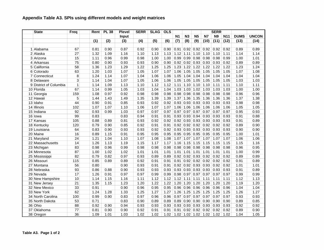
Appendix Table A3. SPIs using different models and weight matrices

State Freq Rent PL 38 Plevel SERR SLAG OLS SERRInput N1 N3 N5 N7 N9 N11 DUMS UNCON

(1) (2) (3) (4) (5) (6) (7) (8) (9) (10) (11) (12) (13) (14)

1 Alabama 67 0.81 0.90 0.87 0.92 0.90 0.90 0.91 0.92 0.92 0.92 0.92 0.92 0.89 0.892 Alaska 27 1.32 1.09 1.16 1.10 1.13 1.13 1.12 1.11 1.10 1.10 1.10 1.11 1.14 1.143 Arizona 15 1.11 0.96 0.99 0.98 1.00 1.00 0.99 0.99 0.98 0.98 0.98 0.99 1.00 1.014 Arkansas 75 0.80 0.90 0.93 0.93 0.90 0.90 0.92 0.92 0.93 0.93 0.93 0.92 0.89 0.895 California 58 1.36 1.23 1.29 1.22 1.25 1.25 1.23 1.22 1.22 1.22 1.22 1.22 1.23 1.246 Colorado 63 1.20 1.03 1.07 1.05 1.07 1.07 1.06 1.05 1.05 1.05 1.05 1.05 1.07 1.087 Connecticut 8 1.24 1.14 1.07 1.04 1.06 1.06 1.05 1.04 1.04 1.04 1.04 1.04 1.04 1.048 Delaware 3 1.14 1.04 1.07 1.05 1.06 1.06 1.05 1.05 1.05 1.05 1.05 1.05 1.03 1.039 District of Columbia 1 1.14 1.09 1.13 1.10 1.12 1.12 1.11 1.10 1.10 1.10 1.11 1.11 1.10 1.11

10 Florida 67 1.14 0.99 1.05 1.03 1.04 1.04 1.03 1.03 1.02 1.03 1.03 1.03 1.00 1.0011 Georgia 159 1.08 0.97 0.92 0.98 0.98 0.98 0.98 0.98 0.98 0.98 0.98 0.98 0.96 0.9612 Hawaii 5 1.44 1.43 1.49 1.35 1.39 1.39 1.37 1.36 1.35 1.36 1.36 1.36 1.37 1.3813 Idaho 44 0.90 0.91 0.85 0.93 0.92 0.92 0.93 0.93 0.93 0.93 0.93 0.93 0.98 0.9814 Illinois 102 1.07 1.07 1.10 1.06 1.07 1.07 1.06 1.06 1.06 1.06 1.06 1.06 1.05 1.0515 Indiana 92 0.93 0.99 1.03 0.97 0.97 0.97 0.97 0.97 0.97 0.97 0.97 0.97 0.95 0.9316 Iowa 99 0.83 0.83 0.94 0.91 0.91 0.93 0.93 0.94 0.93 0.93 0.93 0.91 0.8817 Kansas 105 0.88 0.89 0.81 0.93 0.92 0.92 0.92 0.93 0.93 0.93 0.93 0.93 0.91 0.8918 Kentucky 120 0.79 0.90 0.85 0.92 0.91 0.91 0.92 0.92 0.92 0.92 0.92 0.92 0.89 0.9019 Louisiana 64 0.83 0.90 0.93 0.93 0.92 0.92 0.93 0.93 0.93 0.93 0.93 0.93 0.90 0.9020 Maine 16 0.89 1.15 0.91 0.95 0.95 0.95 0.95 0.95 0.95 0.95 0.95 0.95 1.00 1.0121 Maryland 24 1.21 1.04 1.10 1.07 1.08 1.08 1.07 1.07 1.07 1.07 1.07 1.07 1.06 1.0622 Massachusetts 14 1.26 1.13 1.19 1.15 1.17 1.17 1.16 1.15 1.15 1.15 1.15 1.15 1.15 1.1623 Michigan 83 0.98 0.96 0.99 0.98 0.98 0.98 0.98 0.98 0.98 0.98 0.98 0.98 0.96 0.9524 Minnesota 87 1.00 1.02 1.02 1.01 1.01 1.01 1.01 1.01 1.01 1.01 1.01 1.01 1.00 0.9925 Mississippi 82 0.79 0.82 0.97 0.93 0.89 0.89 0.92 0.92 0.93 0.92 0.92 0.92 0.89 0.8926 Missouri 115 0.85 0.89 0.89 0.92 0.91 0.91 0.91 0.92 0.92 0.92 0.92 0.92 0.91 0.8927 Montana 56 0.80 0.90 0.93 0.91 0.91 0.92 0.92 0.93 0.93 0.92 0.92 1.01 1.0128 Nebraska 93 0.86 0.88 0.90 0.93 0.93 0.93 0.93 0.93 0.93 0.93 0.93 0.93 0.91 0.8929 Nevada 17 1.26 0.91 0.97 0.97 0.99 0.99 0.98 0.97 0.97 0.97 0.97 0.97 0.99 0.9930 New Hampshire 10 1.14 1.15 1.16 1.11 1.12 1.12 1.12 1.11 1.11 1.11 1.11 1.11 1.12 1.1331 New Jersey 21 1.35 1.15 1.23 1.20 1.22 1.22 1.20 1.20 1.20 1.20 1.20 1.20 1.19 1.2032 New Mexico 33 0.91 0.90 0.96 0.95 0.95 0.96 0.96 0.96 0.96 0.96 0.96 1.04 1.0433 New York 62 1.24 1.28 1.33 1.25 1.27 1.27 1.26 1.25 1.25 1.25 1.25 1.25 1.26 1.2734 North Carolina 100 0.99 0.90 0.83 0.97 0.96 0.96 0.97 0.97 0.97 0.97 0.97 0.97 0.93 0.9335 North Dakota 53 0.71 0.83 0.90 0.89 0.89 0.89 0.90 0.90 0.90 0.90 0.90 0.89 0.8536 Ohio 88 0.92 0.90 0.94 0.93 0.93 0.93 0.93 0.93 0.93 0.93 0.93 0.93 0.92 0.9237 Oklahoma 77 0.81 0.90 0.90 0.92 0.91 0.91 0.91 0.92 0.92 0.92 0.92 0.92 0.89 0.9038 Oregon 36 1.09 1.01 1.03 1.02 1.02 1.02 1.02 1.02 1.02 1.02 1.02 1.02 1.04 1.05

Table A3. Page 1 of 2

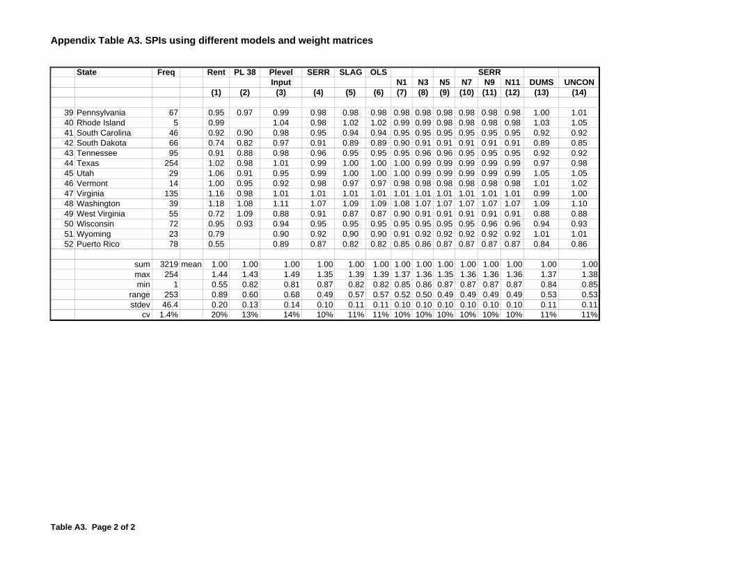
Appendix Table A3. SPIs using different models and weight matrices

State Freq Rent PL 38 Plevel SERR SLAG OLS SERRInput N1 N3 N5 N7 N9 N11 DUMS UNCON

(1) (2) (3) (4) (5) (6) (7) (8) (9) (10) (11) (12) (13) (14)

39 Pennsylvania 67 0.95 0.97 0.99 0.98 0.98 0.98 0.98 0.98 0.98 0.98 0.98 0.98 1.00 1.0140 Rhode Island 5 0.99 1.04 0.98 1.02 1.02 0.99 0.99 0.98 0.98 0.98 0.98 1.03 1.0541 South Carolina 46 0.92 0.90 0.98 0.95 0.94 0.94 0.95 0.95 0.95 0.95 0.95 0.95 0.92 0.9242 South Dakota 66 0.74 0.82 0.97 0.91 0.89 0.89 0.90 0.91 0.91 0.91 0.91 0.91 0.89 0.8543 Tennessee 95 0.91 0.88 0.98 0.96 0.95 0.95 0.95 0.96 0.96 0.95 0.95 0.95 0.92 0.9244 Texas 254 1.02 0.98 1.01 0.99 1.00 1.00 1.00 0.99 0.99 0.99 0.99 0.99 0.97 0.9845 Utah 29 1.06 0.91 0.95 0.99 1.00 1.00 1.00 0.99 0.99 0.99 0.99 0.99 1.05 1.0546 Vermont 14 1.00 0.95 0.92 0.98 0.97 0.97 0.98 0.98 0.98 0.98 0.98 0.98 1.01 1.0247 Virginia 135 1.16 0.98 1.01 1.01 1.01 1.01 1.01 1.01 1.01 1.01 1.01 1.01 0.99 1.0048 Washington 39 1.18 1.08 1.11 1.07 1.09 1.09 1.08 1.07 1.07 1.07 1.07 1.07 1.09 1.1049 West Virginia 55 0.72 1.09 0.88 0.91 0.87 0.87 0.90 0.91 0.91 0.91 0.91 0.91 0.88 0.8850 Wisconsin 72 0.95 0.93 0.94 0.95 0.95 0.95 0.95 0.95 0.95 0.95 0.96 0.96 0.94 0.9351 Wyoming 23 0.79 0.90 0.92 0.90 0.90 0.91 0.92 0.92 0.92 0.92 0.92 1.01 1.0152 Puerto Rico 78 0.55 0.89 0.87 0.82 0.82 0.85 0.86 0.87 0.87 0.87 0.87 0.84 0.86

sum 3219 mean 1.00 1.00 1.00 1.00 1.00 1.00 1.00 1.00 1.00 1.00 1.00 1.00 1.00 1.00max 254 1.44 1.43 1.49 1.35 1.39 1.39 1.37 1.36 1.35 1.36 1.36 1.36 1.37 1.38min 1 0.55 0.82 0.81 0.87 0.82 0.82 0.85 0.86 0.87 0.87 0.87 0.87 0.84 0.85

range 253 0.89 0.60 0.68 0.49 0.57 0.57 0.52 0.50 0.49 0.49 0.49 0.49 0.53 0.53stdev 46.4 0.20 0.13 0.14 0.10 0.11 0.11 0.10 0.10 0.10 0.10 0.10 0.10 0.11 0.11

cv 1.4% 20% 13% 14% 10% 11% 11% 10% 10% 10% 10% 10% 10% 11% 11%

Table A3. Page 2 of 2

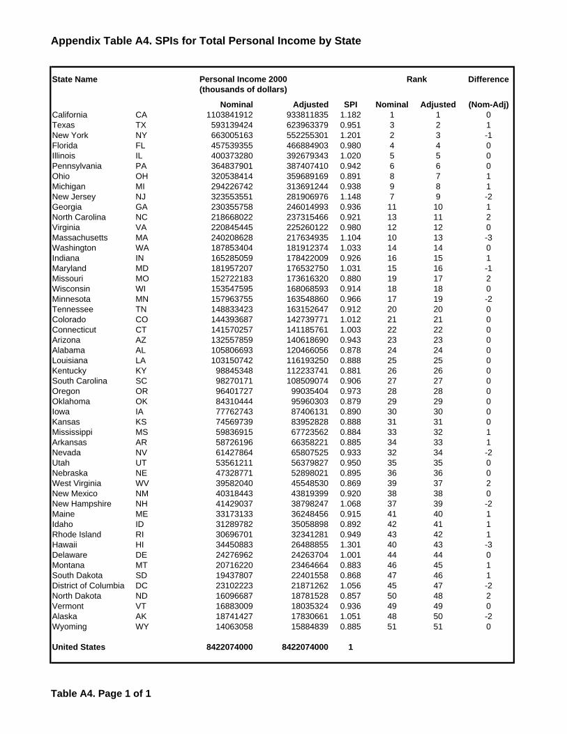
Appendix Table A4. SPIs for Total Personal Income by State

State Name Difference

Nominal Adjusted SPI Nominal Adjusted (Nom-Adj)California CA 1103841912 933811835 1.182 1 1 0Texas TX 593139424 623963379 0.951 3 2 1New York NY 663005163 552255301 1.201 2 3 -1Florida FL 457539355 466884903 0.980 4 4 0Illinois IL 400373280 392679343 1.020 5 5 0Pennsylvania PA 364837901 387407410 0.942 6 6 0Ohio OH 320538414 359689169 0.891 8 7 1Michigan MI 294226742 313691244 0.938 9 8 1New Jersey NJ 323553551 281906976 1.148 7 9 -2Georgia GA 230355758 246014993 0.936 11 10 1North Carolina NC 218668022 237315466 0.921 13 11 2Virginia VA 220845445 225260122 0.980 12 12 0Massachusetts MA 240208628 217634935 1.104 10 13 -3Washington WA 187853404 181912374 1.033 14 14 0Indiana IN 165285059 178422009 0.926 16 15 1Maryland MD 181957207 176532750 1.031 15 16 -1Missouri MO 152722183 173616320 0.880 19 17 2Wisconsin WI 153547595 168068593 0.914 18 18 0Minnesota MN 157963755 163548860 0.966 17 19 -2Tennessee TN 148833423 163152647 0.912 20 20 0Colorado CO 144393687 142739771 1.012 21 21 0Connecticut CT 141570257 141185761 1.003 22 22 0Arizona AZ 132557859 140618690 0.943 23 23 0Alabama AL 105806693 120466056 0.878 24 24 0Louisiana LA 103150742 116193250 0.888 25 25 0Kentucky KY 98845348 112233741 0.881 26 26 0South Carolina SC 98270171 108509074 0.906 27 27 0Oregon OR 96401727 99035404 0.973 28 28 0Oklahoma OK 84310444 95960303 0.879 29 29 0Iowa IA 77762743 87406131 0.890 30 30 0Kansas KS 74569739 83952828 0.888 31 31 0Mississippi MS 59836915 67723562 0.884 33 32 1Arkansas AR 58726196 66358221 0.885 34 33 1Nevada NV 61427864 65807525 0.933 32 34 -2Utah UT 53561211 56379827 0.950 35 35 0Nebraska NE 47328771 52898021 0.895 36 36 0West Virginia WV 39582040 45548530 0.869 39 37 2New Mexico NM 40318443 43819399 0.920 38 38 0New Hampshire NH 41429037 38798247 1.068 37 39 -2Maine ME 33173133 36248456 0.915 41 40 1Idaho ID 31289782 35058898 0.892 42 41 1Rhode Island RI 30696701 32341281 0.949 43 42 1Hawaii HI 34450883 26488855 1.301 40 43 -3Delaware DE 24276962 24263704 1.001 44 44 0Montana MT 20716220 23464664 0.883 46 45 1South Dakota SD 19437807 22401558 0.868 47 46 1District of Columbia DC 23102223 21871262 1.056 45 47 -2North Dakota ND 16096687 18781528 0.857 50 48 2Vermont VT 16883009 18035324 0.936 49 49 0Alaska AK 18741427 17830661 1.051 48 50 -2Wyoming WY 14063058 15884839 0.885 51 51 0

United States 8422074000 8422074000 1

Personal Income 2000 Rank(thousands of dollars)

Table A4. Page 1 of 1