Using Four Corners to Import Goods:

Estimates for Wal-Mart

Thomas J. Holmes* and Ethan Singer**

June 13, 2016

*University of Minnesota and Federal Reserve Bank of Minnapolis

**University of Minnesota

Note: This paper is preliminary and is circulated as part of a conference presentation.

Please do not cite.

We thank Dominic Smith and Jonathan Williard for their research assistance on this

project. The views expressed herein are those of the authors and not necessarily those of

the Federal Reserve Bank of Minneapolis, the Federal Reserve Board or the Federal Reserve

System.

1 Introduction

A container bearing imports from Asia, after being unloaded at a U.S. port, generally makes

a first stop at a firm’s import distribution center (DC), where the container is unpacked,

and the goods are routed through the firm’s distribution network downstream. A firm with

limited scale will generally have only a single import DC. The leading retailers in the U.S.,

such as Wal-Mart, Target, K-Mart, and Home Depot, have enormous scale, and in recent

years have adopted what is called a “four corners” strategy with at least four import DCs,

spread out across the West and East coasts. This strategy lowers a firm’s transportation

costs compared with using a single import DC, since using both coasts makes greater use of

cheap ocean transport. In addition, the stategy potentially makes a firm less vulnerable to

a disruption, such as a labor union strike, at a particular port or distribution center. If a

firm is dependent upon a single port and a single import DC, a disruption at either point

can shut down the firm’s entire operation.

In this paper, we examine a firm’s use of a four corners import strategy. Our first

objective is to develop and estimate a model of the import process. Second, we use the

model to examine what the firm gains by adopting a four corners approach, both in terms of

savings in transportation, and in terms of reducing its vulnerability to disruption. Third,

we examine how adoption of a four corners approach affects which locations are choosen for

port and distribution center activites; this is of interest because port and distribution center

activity at a location potentially connect with a location’s growth.

Our empirical application is the import distribution system of Wal-Mart, which by far is

the largest importer of containers into the United States. We have collected a unique micro

data set with a list of 1.7 million 40-foot containers imported by Wal-Mart over the period

2007 through 2015. Our sample consists of a little more than half of all Wal-Mart’s ocean

container imports over the period. The data includes details such as where each container

originated, the ship used, the foreign and domestic ports, and the import DC receiving

the container. We have information about the contents of the container, specifically for

most records we observe the product item number that Wal-Mart uses to track products,

as well as product classification information. Thus we are able to determine the quantity

allocations across DCs at the product item level. We have merged the shipment records with

GPS information on port calls by vessels, through which we calculate transit times for ocean

voyages. To estimate our model, we also make use of container-level data that we have

constructed on ocean freight expenditures.

1

In the model, the firm first chooses how many import DCs to use and where to put them,

second how to allocate quantities of imports across DCs, and third which ports to use to

get the desired allocation shares to each DC. We highlight two key aspects of the allocation

share choice problem. The first concerns the degree to which the shares are optimized at

the source country level. Retailers like Wal-Mart import goods from a variety of different

countries that can vary in their relative proximity to the East and West coasts. In particular,

China is relatively close to the West Coast and gets to the East coast via the Panama Canal.

Indian Ocean countries are relatively close to the East Coast, and get there via the Suez

Canal. We ask whether Wal-Mart customizes its DC allocation shares for the goods from

individual source countries, to optimize to source country relative transportation cost. Or

do the scale economies of treating the goods from each source country the same at a DC

center outway the gains from customization? We find the latter. DC allocation shares tend

to be invariant across source country. However, the ports used to get to a particular DC can

vary across source countries, and through this margin alone, we show the firm is able to get

quite close to the what the optimum would be with full customization. Take, for example,

the case of India. If Wal-Mart could customize DC allocation shares specifically for India,

it would lower average transportation costs from India aby about one percent. For China

imports, it would be just a tiny fraction of that, because with China’s huge share of import

volume, Wal-Mart essentially optimizes its network to China.

The second share allocation issue that we address concerns what happens when there is

a supply disruption. In the very short run, can the firm adjust DC allocation shares? We

study this issue by examining Wal-Mart’s behavior during the West Coast port slowdown

that occurred at the end of 2014 and beginning of 2015. We find there was no short-run

response in DC allocation shares. However, there is a short-run response in port choice.

That is, we get an analogous result to our finding about sensitivity to country of origin: DC

allocation shares are not flexible, but port choice is.

There are good reasons to believe miminizing vulnerability to disruption is a key consid-

eration in the design of a supply chain of a large retailer. Import channels are a chokepoint,

and if workers can shut down goods flow at a chokepoint, everything stops all the way down

the supply chain, giving the workers tremendous leverage. While as a general rule union

power has declined significantly in the United States, dockworkers have maintained signifi-

cant power, sitting at a chokepoint on top of a distribution pyramid of billions of dollars of

goods flow. In 2002, a labor disruption completely shut down West Coast ports for 11 days.

Goods began to move when President Bush intervened, but goods flow was backlogged for

2

months. Import DCs are also a chokepoint, and Wal-Mart takes steps to keep unions out,

including having them operated by third party firms, who in term hire temporary workers.1

(Even so there was a strike in one import DC and a slowdown in another, two of the few

instances of work stoppages at any Wal-Mart facility.) We use the estimated model to

evaluate the degree to which adoption of a four corners stategy reduces a firm’s vulnerability

to disruption. In particular, after the 2002 West Coast shutdown, Wal-Mart expanded its

import DC network by adding two central DCs in Houston and Chicago, to the one previous

on the West Coast (Los Angeles) and two previous on the East Coast (Savannah, Georgia,

and Norfolk, Virginia). Figure 1 illustrates the loction of the five DCs, as well as estimated

market areas for each DC. We find that despite the addition of the two new DCs, Wal-Mart

remains vulnerable to disruption. The problem is first, in the short run, Wal-Mart cannot

quickly adjust its allocation shares across DCs. Second, it needs to get goods to the West

Coast, and when the West-Coast ports go on strike, there are little in the way of practical

alternatives.

We find that the benefit to Wal-Mart of expanding its distribution to five DCs (which

we think of as adopting the four corner strategy) relative to its 3-DC system is a substantial

reduction in per container cost, on the order of $200 per container (with the exact number

depending upon the origination country). This is approximately 5 to 10 percent of cost.

Moreover, the reduction in cost in going from a 1-DC system to a 3-DC system is the

same order of magnitude. Our calculations do not include the fixed cost of setting up the

additional DCs. Nevertheless, conditional on adoption, the marginal cost is the crucial

cost that feeds into the volume of activity. Our calculations suggest that adoption of four

corner import strategies by large retailers has played an important role in reducing marginal

transportation costs.

1.1 Some Previous Literature

In addition to freight cost, our analysis takes into account the value of time and an important

predecessor paper on time is Hummels and Schaur (2013). This previous paper uses public

census tabulations on how imports enter by mode (in particular, air versus water), and

by port of entry (in particular, West Coast versus East Coast). The paper controls for

1In contrast, Wal-Marts regular distribution centers are all directly run by Wal-Mart with their own

employees. Wal-Mart has significant redundancy in its regular distribution system (e.g. it has 42 general

distribution centers) and if one is shut down because of labor unrest is can substitute other neighboring DCs.

3

particular products, and examines the tendency to substitute away from water towards air,

for deliveries of the particular product to the coast opposite to the originating country (i.e.

the East Coast from Asia, or the West Coast from Europe). We highlight three ways our

paper is different. First, while the previous paper considers the margin of air versus water,

in our paper all the imports are waterborne, and the margin is which ports and DCs to use.

We think this is a good margin to focus on, because it is relevant for a substantial fraction

of import activity. Second, in Hummels and Schaur, the geographic structure is two points,

East and West Coast, and no internal transportation cost is considered. In our paper, we

consider a rich geography and jointly study domestic transportation cost as well as foreign

transportation cost. Third, while we also make some use of published census tabulations

of aggregated data, our main focus is on rich micro data.

Our micro data are the bills of lading filed with the U.S. Customs and Border Patrol

(CBP) as part of the customs process. There is a recent international trade literature

(see Bernard et al (2007, 2009, 2010)) that has linked confidential customs data to firm-level

information. Unlike this earlier literature, we are interested in the specifics of the geography

of where goods arrive. Moreover, by using the publicly available bills of lading data rather

than the confidential data, we are able to report firm-level estimates.

Our paper is part of a recent literature integrating the analysis of international trade

with intra-regional trade. See, for example, Holmes and Stevens (2014), and Cosar and

Fajgelbaum (forthcoming). More broadly, it is part of an emerging literature aiming to

estimate tractable, yet highly detailed models of economic geography, including Ahlfeldt et

al (2016), and Allen and Arkolakis (2014), and recent work specially aiming to quantify

intraregional trade frictions, such as Atkin and Donaldson (2015).

There is extensive analysis of port choice in operations research. Leachman and David-

son (2012), for example, explicitly consider Wal-Mart’s port choice problem in a calibrated

model.2 A key difference here is the way we take a revealed preference approach, estimating

parameters based on Wal-Mart’s behavior.

2See Fradley and Guerrero (2010) for an overview of what is called the global replenishment problem. See

also Veldman and Bückmann (2003) and Veldman and van Drunen (2011).

4

2 Model

2.1 Description of the Model

Consider the problem of a firm that imports a variety of products which it distributes across a

variety of domestic locations. Starting at an originating foreign location, goods are shipped

across the ocean, and unloaded at a domestic port of entry. Next goods are transferred

to an import distribution center, where they are processed and then sent further down the

distribution pipeline, which in general might include secondary, regional distribution centers.

For simplicity, we will abstract from secondary distribution centers, and we will treat the

primary distribution centers (i.e. the import distribution centers which are the first stop) as

distributing goods to the ultimate consumers. This is a reasonable abstraction for Wal-Mart,

because it has a large network of 42 secondary distribution centers for general merchandise,

that are relatively close to the ultimate retail locations that they serve. (See Holmes (2011)

for an analysis of Wal-Mart regional distribution centers.)

Formally, products are indexed by , foreign source locations by , domestic ports by ,

distribution centers (henceforth “DCs”) by , and ultimate consumer locations by , and we

let , , , , denote the counts of goods, foreign locations, domestic ports, DCs, and

ultimate consumer locations. We assume for each product , the foreign source location

is unique, and we write it (). We can show that this is the usual case in our empirical

application.

Firms pay freight costs to move goods from one transportation node to the next. We

define the units of a product on the basis of volume, because that is how transportation is

priced in the empirical application. Specifically, define one unit of a product to be one cubic

meter. Let ( ) be the freight cost in dollars to move one cubic meter from node to

node . If goods start at foreign source and get to ultimate location by going through

port and DC , then the freight cost of this journey in dollars for one unit of the good (i.e.

one cubic meter) is

total freight cost (dollars per unit) = ( ) + ( ) + ( ).

Analogously, let ( ) be the elapsed time taken to go from to , measured in units of

days. Letting be the dollar cost of one extra day to deliver one cubic meter of good ,

5

the time cost in dollars is

total time cost (dollars per unit) = [( ) + ( ) + ( )] .

There are also port and DC-specific costs, each with a deterministic and random compo-

nent. To introduce the random component, let each unit of a good be indexed by . The

port-specific cost of moving unit through port is

+ ,

while the DC-specific cost to move unit through is

+ .

The deterministic port-cost component accounts for any additional direct dollar costs

not included in the freight rate, such as port-specific container taxes, as well as the dollar

value of any implicit costs of using a particular port, such as congestion associated with a

port. The deterministic DC-specific cost of using DC accounts for wage differences

across locations and concerns about unionization, and can also vary across locations to reflect

different investments the firm might have made across DCs that affect DC marginal cost.

Let the random DC cost component be drawn i.i.d. across units and DCs , from

the type-one extreme value distribution with standard deviation . For now, make a similar

assumption on the random port-cost component , setting the standard deviation at .

(In the estimation we will modify this assumption, to have the random draw take place at

the container level rather than the cubic meter level.)

Putting all of this together, the total cost to move unit of good from foreign location

through port and DC to ultimate location is

= ( ) + ( ) + ( ) + [( ) + ( ) + ( )] + + + + .

We take demand at each location as given. Specifically, the firm solves a planning prob-

lem to deliver units of good to location . To allow for demand shocks across locations,

assume is drawn from a distribution Φ(), with mean . We assume a flexible

6

distribution and do not rule out correlation in the realization of these draws across nearby

locations. We assume the firm observes the draw of before making order decisions.

In our assumptions about timing, we want to take into account that setting up a dis-

tribution network is a more longer term decision than port choice. This motivates our

assumption to allow port choices to be made after observing the port random shock ,

while decisions about what distribution center to use is made before this realization. An-

other thing we desire to capture in our model is to parameterize the degree to which a firm

can customize its supply chain from the distribution center onward for particular products.

In one extreme case there is no customization. In this case, a given DC ships the products it

carries to the same set of downstream locations in a similar way. This will be the case when

economies of scale are important, making it cost efficient to run a homogenous distribution

network. In the opposite extreme case, different products get treated differently in the

same DC. There may be an incentive to do this, if scale economies are not important, and

if the same distribution center carries goods from very different originating countries. For

example, suppose there is one DC on the East Coast, and another on the West Coast and

suppose there is one good (product “E”) from a country near the East Coast, and a second

product (“W”) produced near the West Coast. If product-level customization is feasible, it

might be desirably to have the East Coast DC reach further into the interior with product

compared to product . That is, the optimal allocation shares are likely to differ.

To formalize this in the model, assume for each good and each location , there is a

probability that the firm can customize how goods leave the DC to get to the ultimate

location, and with complementary probability 1− the supply chain is constrained to treat

goods sent to location the same way, regardless of origination. Formally, assume in the

event the firm is able to customize distribution of product , the firm picks , the share of

good supplied by DC to location , = 1 . In the event the firm is constrained to

treat all goods the same way, the firm selects a share ◦ from to that does not depend

upon .

2.2 Port-Choice Problem

We begin the analysis of the firm’s problem with the port choice decision. The timing is

such that when the port decision is made, the firm has already determined for each good

the allocation of deliveries across DCs. Hence, in the port decision, we take as given that a

particular unit of product is being shipped to DC . Thus costs at the DC onward can

7

be taken as fixed. At this point, we need only to focus on the cost of getting to the DC.

Consider unit of a good that needs to be shipped to . The cost of using port is

= ( ) + ( ) + [( ) + ( )] + +

= +

where we gather the deterministic components of cost into . For each destination DC

, we allow for the fact that some ports may not be economically feasible, and we let Λ()

be the relevant choice set of . The optimal port minimizes

min∈Λ()

+ (1)

The probability port is selected is

=

exp(−

)P

∈Λ()(−

0)

The expected minimized value of cost for delivering goods to DC is

DC = − ln⎛⎝ X

∈Λ()exp

Ã−

!⎞⎠− (2)

where is Euler’s constant.

2.3 The DC Allocation Problem with Product-Level Customiza-

tion

Suppose the supply chain can be customized at the product level. When making the order

decision, the firm first observes , which is the inelastic demand for product that must

be delivered to location . We can write the cost of choosing DC to ship unit as

=

DC + ( ) + ( ) + +

= + .

8

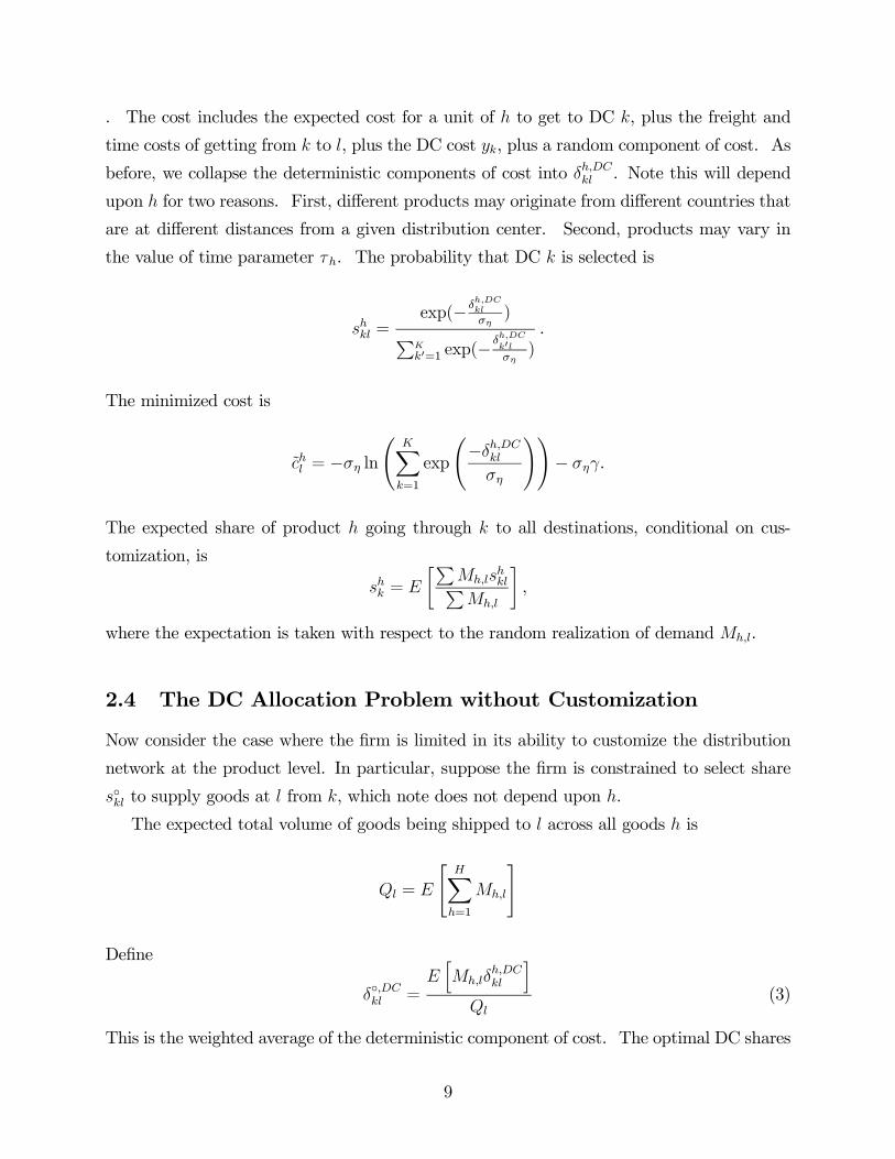
. The cost includes the expected cost for a unit of to get to DC , plus the freight and

time costs of getting from to , plus the DC cost , plus a random component of cost. As

before, we collapse the deterministic components of cost into . Note this will depend

upon for two reasons. First, different products may originate from different countries that

are at different distances from a given distribution center. Second, products may vary in

the value of time parameter . The probability that DC is selected is

=exp(−

)P

0=1 exp(−

0)

.

The minimized cost is

= − lnÃ

X=1

exp

Ã−

!!− .

The expected share of product going through to all destinations, conditional on cus-

tomization, is

=

∙P

P

¸,

where the expectation is taken with respect to the random realization of demand .

2.4 The DC Allocation Problem without Customization

Now consider the case where the firm is limited in its ability to customize the distribution

network at the product level. In particular, suppose the firm is constrained to select share

◦ to supply goods at from , which note does not depend upon .

The expected total volume of goods being shipped to across all goods is

=

"X=1

#

Define

◦ =

h

i

(3)

This is the weighted average of the deterministic component of cost. The optimal DC shares

9

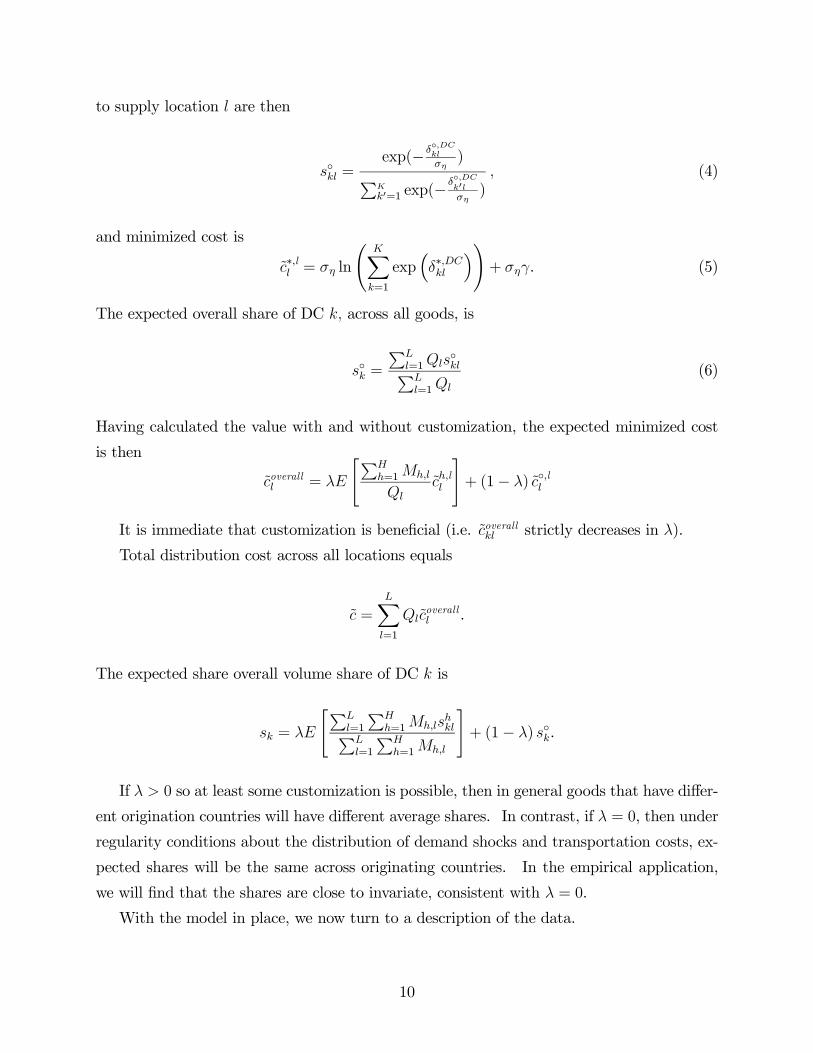
to supply location are then

◦ =exp(−

◦

)P

0=1 exp(−◦0)

(4)

and minimized cost is

∗l = ln

ÃX=1

exp³∗

´!+ . (5)

The expected overall share of DC across all goods, is

◦ =

P

=1◦P

=1

(6)

Having calculated the value with and without customization, the expected minimized cost

is then

overall =

"P

=1

l

#+ (1− )

◦l

It is immediate that customization is beneficial (i.e. overall strictly decreases in ).

Total distribution cost across all locations equals

=

X=1

overall .

The expected share overall volume share of DC is

=

"P

=1

P

=1P

=1

P

=1

#+ (1− ) ◦.

If 0 so at least some customization is possible, then in general goods that have differ-

ent origination countries will have different average shares. In contrast, if = 0, then under

regularity conditions about the distribution of demand shocks and transportation costs, ex-

pected shares will be the same across originating countries. In the empirical application,

we will find that the shares are close to invariate, consistent with = 0.

With the model in place, we now turn to a description of the data.

10

3 Data

3.1 Bill of Lading Data

The U.S. Department of Customs and Border Protection (CBP) releases detailed information

about bills of lading of waterborne imports. A bill of lading is a document issued by a carrier

that provides details of the shipment. The CBP sells the raw data to various shipping

information companies who then resell the data. We have accessed this data through a

subscription to Ealing Market Data Engineering. Over the period 2007 through 2015 that

we consider, there are typically a little more than one million bills of lading each month.

Table 1 illustrates information from two example bills of lading, one for a shipment of

children’s car seats, another for a shipment of 50-inch HD TVs. The place of receipt is listed,

as well as the foreign port where the shipment was laded onto the vessel. These happen

to be the same for the two examples, but will differ when the place of receipt is inland, or

when there is transshipment at a hub port.3 For example, goods originating in Bangladesh,

destined for West Coast U.S. ports, are frequently transhipped in Singapore, which is then

listed as the foreign port. The record specifies the name of the vessel carrying the shipment

to the U.S., as well as the arrival date. The port of unlading is the location where the

shipment was unloaded off the vessel and the port of entry is where the shipment clears

customs. These generally differ for intermodal shipments. For example, the car seat record

indicates that the shipment was unladed in Los Angeles, and was then shipped (presumably

by rail) to Houston, where it went through customs. For the TVs, the ports of unlading and

entry are both Norfolk.

In the car seat example, the shipper is listed as the Evenflo Company (a manufacturer

of car seats), and the consignee is listed as Wal-Mart. Shippers and consignees may request

that both the shipper and consignee data fields be suppressed. The first record is among

of the rare exceptions where the confidentially option was not chosen by Wal-Mart. Infor-

mation in the remaining fields can potentially be used to identify the shipper or consignee.

Notice, in particular, in the products field for both records, you can see the code “GLN#

0078742000008.” This is the global location number that Wal-Mart uses for shipments with

destinations in the United States. A search for the text pattern “0078742000008” in either

the products field, or in a related field called “marks,” results in 1.5 million bills of lading

3It is important for record keeping that the place of receipt be accurate, because the actual country where

the good originates may affect customs duties, and because transportation costs in moving inland freight is

deductible for customs duties.

11

observations for the period 2007 to 2015. That these are indeed Wal-Mart observations can

be corroborated from other information on the records. Using various other strategies de-

scribed in the appendix, we are able uncover an additional 0.4 million records for a total

sample of approximately 1.9 million Wal-Mart bills of lading.4

All internationally shipped containers have a unique 11 digit identification number (BIC

code) that is maintained by an international registry. Each bill of lading lists the BIC codes

of all the containers that are part of the shipment. The car seat shipment consists of two

containers. There are 417 containers for the TV shipment (this is the maximum container

count across all Wal-Mart shipments in our sample). For each container, the record lists

the piece count, which for Wal-Mart is generally the count of cartons in the container. For

the car seat example, each carton contains a single car seat, and there are 1056 units in each

container. Similarly, for the TVs, each carton is a single TV and there are exactly 297 TVs

in each of the 417 containers. Some web searches show that the original Wal-Mart prices

for these products were $50 for the car seat and $498 for the TVs, which, after multiplying

by the piece counts result in container-level retail values of $53,000 and $148,000 for the car

seats and TVs, and the total retail values of the orders are $103,000 and $62 million.

Volumes per container equal 63 and 65.7 cubic meters in the two examples, which are close

to the maximum usable space of 67.7 cubic feet for a 40ft standard container.5 Weights per

container in the two examples are 4,066, and 5,265 Kg, significantly less than the maximum

container weight of around 25,000 Kg. This illustrates an important point that for the types

of goods Wal-Mart sells, containers hit capacity first in volume instead of weight. Since

container shipping prices do not depend upon weight, transportation cost considerations are

all about the volume of the goods, not the weight. (See also Leachman (2004).) Since the

cubic meter volume measure is missing for many records in the sample, we will use counts

of containers, and allocated portions of containers, as our unit of measure.

We henceforth refer to each individual bill of lading as a shipment. Table 2 tabulates the

distribution of shipment counts and container counts across the nine years in our sample.

One thing to note is that it is common for there to be multiple shipments corresponding

to the same arriving container. This happens when a particular order does not fill up

a container. Wal-Mart will then generally combine orders with different bills of lading

into the same container, to efficiently stuff containers full. Fortunately, we have the BIC

4Note we exclude from this sample 90,000 bills of lading for shipments going to Canada and Mexico that

go through US ports.5See Leachman (2004, p 77).

12

container codes for each shipment, so we can keep track of when Wal-Mart does this. The

total count of unique containers in our sample is 1.7 million, a little less than the bills of

lading count of 1.9 million.6 To get a sense of the coverage of our sample, we compare our

counts with statistics on company-level aggregate annual container imports, published by

PIERS.7 Overall, the container count in our sample is 53 percent of the aggregates reported

by PIERS.8 One potential source of a difference is mistakes in the way the paperwork is

filled out, e.g. the reported GLN may be off by one digit and we miss this. In our statistical

analysis will attempt to take this into account by focusing on products where we think the

measurement error is likely to be small. Another possibility is that different departments

might have different paperwork protocols, e.g., that do not include the GLN, and there are

likely certain categories of goods for which we are missing all the records for all the products.

For much of what we do, this will not be a problem, because we mostly will be conditioning

on particular products, and as we will see, we will have plenty of them.

Table 3 displays the distribution of Wal-Mart container imports across country of origin.

(We use the place of receipt variable to determine this.) We list every origin country with

10,000 containers or more. China completely dominates the list, accounting for 85.7 percent

of all imports. The next highest is Bangladesh with 1.9 percent. Guatemala and Costa

Rica make the list, mostly because of bananas. The rest of the leading countries are from

Asia.

In the example product fields in Table 1, you can see a nine digit “item number.” The

Wal-Mart item number is an internal code the company uses as a stock-keeping unit to keep

track of products. There products field in the examples also contain a ten digit HS product

code that is used as part of customs filing. Finally there is a two-digit code specifying the

department making the order. We have parsed the product field (and the related field called

“marks”) to pull out these codes. For some records there are multiple item numbers, and an

individual item number may appear multiple times in a record. In such cases, we allocate

the piece count of a bill of lading record across item numbers, in proportion to the number of

times the item number appears in the record. In cases where the same container shipment

appears across multiple bills of lading, we allocate the volume of the container in proportion

to piece counts. In the end, we produce a data set disaggregated to the level of an item and

6Note the same container may be used on multiple ocean voyages. Throughout we will refer to the same

containers used on different voyages as different containers.7To produce these estimates, PIERS uses the same bill of lading data from CBP that we have, plus it

uses additional information it obtains directly from shippers.8The exception of 72 percent in 2007 is a result of the fact for that year, there were many observations

where Wal-Mart failed to supress the consignee field.

13

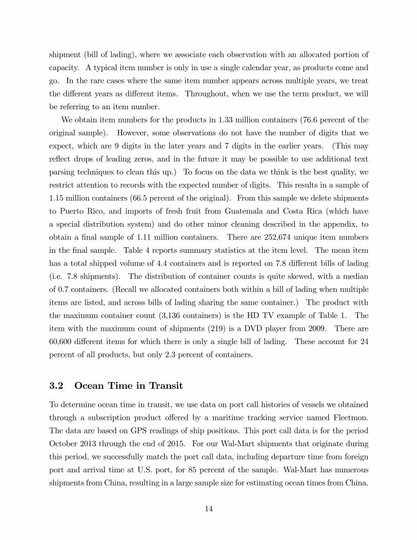
shipment (bill of lading), where we associate each observation with an allocated portion of

capacity. A typical item number is only in use a single calendar year, as products come and

go. In the rare cases where the same item number appears across multiple years, we treat

the different years as different items. Throughout, when we use the term product, we will

be referring to an item number.

We obtain item numbers for the products in 1.33 million containers (76.6 percent of the

original sample). However, some observations do not have the number of digits that we

expect, which are 9 digits in the later years and 7 digits in the earlier years. (This may

reflect drops of leading zeros, and in the future it may be possible to use additional text

parsing techniques to clean this up.) To focus on the data we think is the best quality, we

restrict attention to records with the expected number of digits. This results in a sample of

1.15 million containers (66.5 percent of the original). From this sample we delete shipments

to Puerto Rico, and imports of fresh fruit from Guatemala and Costa Rica (which have

a special distribution system) and do other minor cleaning described in the appendix, to

obtain a final sample of 1.11 million containers. There are 252,674 unique item numbers

in the final sample. Table 4 reports summary statistics at the item level. The mean item

has a total shipped volume of 4.4 containers and is reported on 7.8 different bills of lading

(i.e. 7.8 shipments). The distribution of container counts is quite skewed, with a median

of 0.7 containers. (Recall we allocated containers both within a bill of lading when multiple

items are listed, and across bills of lading sharing the same container.) The product with

the maximum container count (3,136 containers) is the HD TV example of Table 1. The

item with the maximum count of shipments (219) is a DVD player from 2009. There are

60,600 different items for which there is only a single bill of lading. These account for 24

percent of all products, but only 2.3 percent of containers.

3.2 Ocean Time in Transit

To determine ocean time in transit, we use data on port call histories of vessels we obtained

through a subscription product offered by a maritime tracking service named Fleetmon.

The data are based on GPS readings of ship positions. This port call data is for the period

October 2013 through the end of 2015. For our Wal-Mart shipments that originate during

this period, we successfully match the port call data, including departure time from foreign

port and arrival time at U.S. port, for 85 percent of the sample. Wal-Mart has numerous

shipments from China, resulting in a large sample size for estimating ocean times from China.

14

As noted earlier (see Table 3), the sample of shipments from other countries is relatively

small. To estimate travel times to these other countries, we expand the our sample to

include shipments for other firms besides Wal-Mart. Specifically, for the months Nov. 2013

through March 2014, and again Nov 2014 through March 2015, we use the complete set

of all bills of lading. There are 10.8 bills of lading in this sample of ten months of data.

We match the port call time of departure and arrival for approximately 75 percent of these

observations.

3.3 Ocean Freight Rates

We require estimates of ocean freight rates. There exist spot market indices (e.g. the Drewry

World Container Index), but there are two problems using these indices. First, the indices

report spot rates. However, most transactions occur based on contract rates. In particular,

we expect Wal-Mart’s long-run decision making to be based on contract rates. Second, the

available indices are for a limited set of port combinations, and we need freight rates for a

wide set of possible combinations of foreign and domestic ports. A second resource for freight

rates is the published tabulations from the U.S. Census of freight charges based on customs

records. Expenditures on freight are deductible for customs duties, so freight is collected as

part of the administrative procedure. The Census publishes detailed tabulations by narrow

product type, month, and port of unlading and port of entry, and originating country. In

these tabulations, the freight charges, the merchandise values, and the weight (kilograms)

are reported for each of these cells, even if there is only one record (the data also includes a

count of records). While this data is extremely rich, as noted earlier, for the kinds of goods

Wal-Mart sells, freight rates are based on volume not weight.

Our strategy to address this issue is to match the container information in the public

bills of lading, with the freight charge information in the published Census tabulations. The

strategy has several parts, and we explain the details in the appendix. But one of the main

parts of the strategy is link cases in the published tabulations where it is indicated that

there is only a single transaction in that cell. Since the Census tabulation reports weight,

we look for a matching observation in the bills of lading with the same weight in the same

cell (e.g. country of origination, port of unlading, and port of entry). For 18 months, we

have a complete set of bills of lading (17.8 million records) that we use for the matching

exercise. We obtain 140,000 matches of Census data for which we can merge in container

information.

15

3.4 Internal Geography and Ultimate Consumers

For our internal geography, we partition the U.S. according to core-based statistical areas

(CBSAs). For those rural areas outside of CBSA, we allocate them according to BEA

Economic Areas. After we eliminate Alaska, Hawaii, and Puerto Rico, we are left with a

partition of the forty eight contiguous states into 1095 geographic units, that correspond to

the locations indexed by in the model.

Our analysis requires an estimate of the inelastic demand at each domestic location. We

use estimates of Wal-Mart’s store level sales for 2006 from data in Holmes (2011), and make

adjustments for later dates using the distribution of stores in a particular year.

3.5 Domestic Freight and Time

We use Leachman and other sources.

For domestic freight rates we also appeal to worldfreightrates and to the Surface Trans-

portation Board’s public sample of rail waybills. Using the worldfreightrates trucking cost

data we regress truck price on distance, and find an intercept of 141.11 with a per mile cost

of 1.21 (standard errors are 89.04 and 0.052 respectively). The r-squared of this regression

is 0.88. Using the waybill data we regress rail price on distance, and find an intercept of

398.17 with a per mile cost of 0.74, with an r-squared of 0.34

For domestic transit via truck we use driving time estimates between ports and destina-

tions reported by worldfreightrates. To approximate drive times between points for which

we did not collect drive time data, we regress drive time in hours on distance and use the

fitted values. This simple regression has a very good fit with an r-squared of 0.99.9 To get

the total inland transit time for truck shipments, we extend these drive time estimates to

account for driver rest requirements that mandate 10 hour breaks for 11 hours of driving.10

For domestic transit on rail, we use information form published intermodal rail schedules

from the major rail carriers serving ocean ports (Union Pacific, BNSF, CSX, and Norfolk

Southern). Published transit times were available on 365 routes between major ports and

destinations. On routes with multiple trips of different times, the average transit time was

used. While the schedules contain information on transit times for the major rail routes,

9The coefficient on miles is 0.01428 with a standard error of 0.00006, implying an average speed of 70

miles per hour. The intercept was 0.38 with a standard error of 0.096.10The HS code is missing for about 10 percent of our sample and for these records we parts the products

field for fashion good terms like “footwear.”

16

estimates of times between other points are approximated by regressing the scheduled time

on distance and using the fitted values.11

4 Preliminary Analysis

This section establishes facts about Wal-Mart’s behavior. These facts play a role in the

quantitative analysis with the model in the next section.

4.1 Import Distribution Network

Wal-Mart’s strategy for general merchandise imports of using five import distribution centers

is described in MWPVL, and in Leachman. With our data it is easy to see Wal-Mart using

the strategy, as many records list the destination DC in the products or marks field. Also,

the data include port of entry and port of unlading. For example, it is straightforward to see

in the data that containers going through Seattle are virtually all going to the Chicago DC

because (1) most of these records list Chicago as port of entry, and (2) in small percentage

of cases where district of entry is left blank, there typically is indication in the product field

or marks field that the shipment is going to Chicago (or actually Elwood, which is the town

in the Chicago area where the import DC is located.)

Wal-Mart employs different import distribution systems for other classes of products.

In particular, there is a separate system for footwear and clothing (the fashion distribution

system). In addition, there is a system for the Sam’s Club warehouse store format. The

Sam’s club records are identified by the first two digits of the item number being “63.”

Fashion goods are identified by two-digit HS codes 61, 62, and 64, and additional text

information in the products field for when the HS code is missing. General merchandise

is the residual. Table 5 reports the distribution of product counts, shipment counts, and

container counts across these 3 broad groupings of products.

We illustrate the different systems with the following exercise. We start by taking each

product and count the total number of different shipments of the product. Next we calculate

the total number of different destination DCs used for each product. The maximum is five

(5-DC), the minimum is one (1-DC) Table 6 reports the distributions across the count of DCs

reached, and count of product shipments, for both general merchandise and fashion goods.

11The intercept is 46.9 hours (standard error of 3.9) and each mile adds 0.0649 hours (standard error of

0.0026). The r-squared of this regression is 0.63.

17

For goods with only one shipment, 100.0 percent are necessarily 1-DC. With two shipments,

some are 1-DC and others are 2-DC. Inspection of Table 6 reveals clear differences between

general merchandise and fashion. Consider first goods with 5 or more shipments (except

for the case of 6 shipments which we come back to). For General Merchandise, the mode

is 5-DC. In fact, for the 7,858 products with 41 or more shipments, a 0.97 share hit all the

DCs at least once. In contrast, for fashion, the mode outcome is 1-DC. This is true even

for goods with 21-40 shipments. Typically, shipments all go to same distribution center.

The exception for fashion is the category of 41 or more shipments, which only has a few

cases, and these tend to go to all five DCs. Manual inspection of the 5-DC fashion cases

reveals that these are footwear products like “98 cent flipflops” that are being run through

the general merchandise system. Flipflops lack the variety of different sizes that are typical

for footwear, and are therefore more like general merchandise.

Next look at general merchandise products with exactly 5 shipments. For a 0.75 share,

exactly one shipment goes to each DC. There are is also a 0.10 share where 4 DCs are

reached, i.e. one is missed, and another gets two. From manual inspection, we believe that

many of the latter are reporting errors. For example, we see cases where there are two similar

size shipments to Los Angeles, and none to Chicago; we believe that in many of these cases,

one of the two is destined for Chicago, but this was not noted in the paperwork. Next,

observe that cases with 4 product shipments, a 0.75 share hit 4 DCs. In the appendix (to

be completed) we present an argument that this is likely to be measurement error where we

miss a shipment, rather than Wal-Mart actually sending shipments to only 4 DCs, and then

reshuffling to get product to the territory covered by the missing DC. Also, many products we

are classifying as general merchandise that go to only one DC may actually be fashion goods.

For these reasons, in our analysis of general merchandise, we will condition on products with

shipments to all 5 DCs, where we think the data is the best, and this subsample accounts for

75 percent of the containers in our initial general merchandise sample. We also place special

focus on the case where there are exactly 5 shipments, one to each DC. We regard this as a

clean case. These are instances of "one-off" orders where Wal-Mart puts in an order with no

subsequent order for replenishment. As we will show in a later version of the paper, these 5

shipments tend to arrive at approximately the same day to their destination DCs. One-off

situations are relatively common. Notice that the frequency count for 6 shipment products

drops off significantly (There 15,318 with 5 and 3,971 with 6), and moreover these don’t fit

the pattern of a mode point at 5 DCs. Some of these are likely misclassified fashion items.

18

4.2 Order Allocation and Country of Origin

In this subsection we examine how order allocations vary across country of origination, for

destination DCs, and the ports used to get there. For much of the analysis, we group

countries into three geographic categories. The first is China plus Taiwan. To get to East

Coast ports from China or Taiwan, ships generally sail east through the Panama Canal. The

next category includes the remaining countries in lower part of the South China Sea. To

get to the East Coast from here, ships generally sail west, through the Suez Canal. The

third group of countries have ports in the Indian Ocean. For these, sailing time to the East

Coast is less than to the West Coast.

We start by looking at fashion products that are delivered to a single DC. This selection

excludes, for example, the 98 cent flip flops has have the footwear HS code, but are run

through the general merchandise DC system. Table 7 reports the DC shares, by country

grouping, and by individual countries of origin for the entire sample of 79,805 products.

The bottom panel considers the subsample of 15,508 products with five or more shipments.

Consider first the bottom panel, where the pattern is crystal clear. For China and Taiwan,

there is roughly a 50/50 split of Houston or Chicago as the DC. For the South China Sea

category, Chicago’s share drops close to zero, and Houston’s share rises all the way to 0.80.

These countries are further south than China, making Chicago less desirable. Also, Houston

is relatively closer, and the option value of being able to get to Houston through LA from the

west, or from the east through the Suez canal is valuable. And notice that Savannah’s share

creeps up to 0.16, which is the East Coast option, as opposed to the more central Houston

option. Finally, for the Indian Ocean countries, which are relatively close to the Suez Canal,

virtually all (0.98 share) are shipped to the East Coast DC at Savannah. When we look

at the top panel that includes products with less than 5 shipments, and the breakdown by

individual countries, there is noise as some of the smaller cases with few shipments results

in some spreading across the DC, i.e. the Savannah share for Indian Ocean countries is 0.81

rather than 0.98. Nonetheless, the overall pattern remains clear. The allocation choice of

the single destination DC for handling a particular fashion good depends significantly on the

location of the originating good.

Next in Table 8, we report DC share allocation for general merchandise products. We

condition on products with deliveries to all 5 DCs, for which the data quality is best. The

table reports mean share allocations by country. The mean shares are remarkably similar

across countries. In the bottom panel, we consider the “one-off” subsample, where there is a

19

single shipment for each product to each DC. Above we argued that this subsample is likely

to be particularly clean. We can see that the pattern of allocation shares being constant

across the geographic groups is particularly sharp. When we go to our quantitative analysis

in the next section , we take Table 8 as evidence consistent with the customization ability

parameter in our model being zero.

So far we have looked at allocation of deliveries across DCs. Next we turn to the port

choice decision. The Los Angeles, Savannah, and Norfolk DCs obtain virtually all of their

deliveries from their nearby port. The Houston DC is at a port on the Gulf of Mexico,

and obtains direct shipments that way, but also being central (compared to Savannah and

Norfolk which are east), it is can also be reach by shipments to Los Angeles and rail for the

rest of the way, and so a port choice needs to be made. For the Chicago DC there is no

ocean port, and shipments go through Seattle or Los Angeles from the west, or generally

New York from the east.12

Table 9 reports what ports are used to get to Houston and Chicago for the two classes of

products, by source. For fashion to Houston from China, and the South China Sea there is

roughly a half and half split between Los Angeles and Houston. And to Chicago virtually

all of the goods go through Seattle. As noted above, fashion goods from the Indian Ocean

generally not go to either Chicago or Houston (Savannah of the usual destination). For the

few exception, the choice for Houston is to go their directly rather than through Los Angeles,

and to get to Chicago, Los Angeles is the typical choice.

Turning to port choice for general merchandise, again we see that port choice is highly

sensitive to origination. In particular, from the Indian Ocean, East Coast ports are relatively

closer than the West Coast, so the Port of Los Angeles is less likely to be chosen compared

to port choice with shipments from China or the South China Sea.

4.3 Order Allocation in Response to a Temporary Port Shock

Next we consider how order allocations respond to a port shock, in terms of destination DCs

and ports that are chosen. In particular, we examine the West Coast dock slowdown that

occurred between 2014 and early 2015. The contract expired July 1, 2014 and the workers

continued to work without a contract. Late in 2014 slowdowns began to occur. There were

arguments between management and labor as to why these occurred. Work slowed down

12Shipments to Chicago from the east sometimes also go throught Norfolk, but for simplicity we are going

to treat these as going through New York.

20

dramatically in early 2015, and the labor issues were eventually settled on February 20, but

there were several months of congestion after the settlement to work through the backlog.13

We can use our matched shipment/port-of-call data to measure the extent of the slow-

down. We take our Wal-Mart data set, and work with the data at the container level. For

each container, we know the vessel carrying it, and with the port-of-call data we determine

the time of departure from the foreign port and the time of arrival at the domestic port. We

take the difference and call this the voyage duration. Figure 2 plots median duration across

containers to get from Shenzhen or Shanghai to Los Angeles. We aggregate the shipments

to the weekly level, based on the week the container departed from China. We use a one

week ahead and one week behind rolling window, and take the median. We can see the

median duration was between 14 and 15 days throughout most of 2014, until late in the

year. The duration goes up in December, and then explodes to over 30 days in January and

February. It then fell, but remained around 17 days, until August.

Next we consider the containers that Wal-Mart shipped from China (we focus on Shen-

zhen and Shanghai originations) to the Houston DC. As noted above, Wal-Mart chooses

between direct shipment to the port of Houston and intermodal shipment through Los An-

geles. The red line in the figure is a moving average of the share of containers going through

Los Angeles. (Again, week is defined by when the container leaves China.) The share moves

around, but averages about 30 percent. Observe that at the end of October, the share begins

to drop, and falls to zero by the end of December. The share did not go back up again, until

May, when things settled down. The episode clearly illustrates that in a case like Houston

for which there is close substitute port not affected by the slowdown, Wal-Mart can be very

flexible.

The substitution possibilities for getting goods from China to the Los Angeles or Chicago

DCs are more limited. In the height of the stoppage, Wal-Mart actually sent 3 containers to

Chicago via the Houston port, but this is negligible. Wal-Mart also sent 553 containers to

Los Angeles via Oakland, a port Wal-Mart otherwise rarely uses. Oakland is covered by the

same union contract as the other west coast ports, but there was variation in the slowdown

at different ports at different times, allowing for some substitution possibilities.14

Next we consider flexibility of the allocation shares across destination DCs for general

merchandise. Let () be the mean allocation share at DC across goods delivered at time .

13For details, see “Economy Still Reeling from West Coast Slowdown” US NEWs, By Andrew Soergel |Staff Writer Feb. 23, 2016.14During the stoppage some shippers reportedly rerouted containers through Canadian ports and then

used rail to get them to their U.S. destinations. These shipments are not in our sample.

21

For this exercise, we define the delivery date as the average arrival date of the first shipments

to Norfolk and Savannah (we pick the two Atlantic ports because the delivery dates for these

are less likely to be connected to the port disruption on the Pacific). We focus on imports

from China. Figure 3 reports nonparametric estimates of the mean allocation shares for

the 5-shipment ("one-off") sample, the bottom panel reports the same thing for products

with seven or more shipments.15 The red vertical lines indicate January 1 of each year,

beginning with January 2007. The plots for the two samples are quite similar and the most

noticeable pattern is the sharp initial increase in the Chicago share. This DC opened June

2006, and the initial upward trend is consistent with Wal-Mart gradually ramping up its use

of the new DC. The main takeaway from these plots is that the relationships are relatively

smooth functions of time. In particular, we don’t see a collapse of shares for Los Angeles

and Chicago, at the end of 2014, which is what we would expect to see if Wal-Mart could

quickly reoptimize its share allocations in response to the port disruption. It is possible

there might be a slight kink near January 1 in the top panel, with of Houston trending

slightly more upward and Los Angeles trending down, but the magnitudes are quite small.

We will see in the quantitative model that if Wal-Mart could instantaneously adjust its DC

shares, the response would be quite large. We interpret Figure 3 as strong evidence that

Wal-Mart cannot adjust DC allocation shares in the very short run.

5 Quantitative Analysis

Here we undertake our quantitative analysis. Part 1 of this section estimates the parameters

of the port choice problem. Part 2 turns to the DC choice problem. Part 3 puts the

estimated model to work.

5.1 The Port Choice Problem

Consider the port choice problem as specified in (1). Recall the time cost parameter

(dollars per day per container) in this problem is defined as specific to the particular product

Here we will assume that is constant across all general merchandise goods, and is a

constant across fashion goods.

15We also condition on the shares at each DC exceeding 0.10, and total annual shipment be the equivalent

of at least one full container. For the 7 plus sample, we require the first and last shipment be within 60

days.

22

In the analysis of the port problem, we will take as known the ocean trip durations and

freight rates. Besides the time cost, the parameters to be estimated are the and the port

specific costs . There is also a freight and time cost to get from the port to the destination

. It is convenient at this point to specify port specific cost as and let this absorb

the DC-specific cost, as well as all costs to be transferred from port to the DC, including the

cost of rail.

The relevant port choices in our application are for the Chicago and Houston DCs. Goods

destined for Chicago are routed either through Seattle, Los Angeles or New York. For goods

from China, Los Angeles and Seattle are relatively close substitutes, and New York is largely

irrelevant. As we move away from China towards the Indian Ocean and get closer to the Suez

canal, getting to Chicago through the East Coast, the New York option becomes relevant.

Goods destined for the Houston DC are routed either directly to the port of Houston or

through Los Angeles and then use rail the rest of the way. The intermodal option through

Los Angeles saves time but is more expensive.

We comment on identification. The trade-off between time and money in the choice of

whether to use the port of Los Angeles or the port of Houston provides information about the

value of time . A confounding issue is that the full dollar cost of each option is not directly

observed, because of the port/DC specific dollar costs that we treat as unobserved here.

It is key for our identification strategy that different origination countries differ in freight and

time costs to get to each port. This variation across source countries allows us to effectively

difference out the , as we compare the differential choice behavior from source countries

with different geography. Finally, the parameter governs the degree of differentiation

of ports that are otherwise similar in freight and time characteristic. The degree to which

the firm substitutes ports (for example between Los Angeles and Seattle to get to Chicago)

provides information about the parameter.

We estimate the port choice model (1) for several samples: all Wal-Mart shipments,

general merchandise and fashion. The samples and estimates are listed in Table 10. Note,

it is necessary to make a normalization in each choice set, and we set equal to zero

for when Los Angeles is used to reach the distribution center. The cost units for the

estimates are on a container basis and the value of time estimates are on a per container per

day basis. The value of time for general merchandise, at $12 per container per day, is much

lower than the value of time for fashion goods which is estimated at $92 per container per day.

For the general merchandise sample, the estimate for is $814 less

which represents the increased cost of using intermodal transportation from Los Angeles

23

compared to going through the Panama Canal. In addition to intermodal cost differences,

the parameters also include any differences in port costs. Turning to the port estimates

for shipments going to the Chicago DC, the port of New York is $256 less costly than Los

Angeles and the port of Seattle is $1 more expensive than sending the shipment through Los

Angeles. Later we can use our micro data (matched container to Census) to say a little

more.

With our parameter estimates we can use formula (2) to calculate the expected minimum

cost to get to from each country. We use these estimates as an input to the DC choice

problem.

5.2 DC Choice Problem

Now we turn to the DC choice problem developed in subsections 2.3 and 2.4. The problem

is to solve the optimal allocation of shares across DCs, for each ultimate destination. A key

parameter in this problem is , which governs the extent the firm can customize allocation

shares to individual originating countries. Based on our finding that Wal-Mart sets the same

shares independent of origin, we take = 0 as our estimate for this parameter.

The only parameters left to be determined are the DC specific costs , and the dif-

ferentiation parameter . We don’t have any direct information on so for our initial

analysis we treat it as equal to the differentiation parameter for ports, and for robustness

we consider alternative values.

We estimate the model for general merchandise. As before, we need to make a nor-

malization and we set = 0. If we take as given values for the remaining parameters,

y = ( , , , ), then we can plug in data on inland freight times and freight

costs, as well as port costs obtained from the previous section, to obtain the DC/ultimate

location level level ◦ given in (3). These are used to obtain DC shares at the local level

(equation (4)) which are then aggregated to the predicted national shares in (6) of

. We estimate y, by taking the observed shares and selecting y to exactly fit the data.

Table 11 presents our estimates of y for general merchandise. The baseline case is where

= , but we also consider variations where is half and where it is twice the level.

In the baseline case, is $141 more expensive than and this reflects the net effect

of the extra intermodal costs of getting to the Chicago DC relative to Los Angeles and the

efficiency differences of the two DCs. The three east cost DCs — Norfolk, Savannah, and

Houston — are all less costly compared to Los Angeles, with Norfolk and Savannah $628 and

24

$918 cheaper while Houston is closer to Los Angeles at an $86 discount. The estimates of y

are qualitatively similar for the other assumptions on .

5.3 Analysis of the Estimated Model

5.3.1 The Gains from a Network of DCs.

We consider how Wal-Mart gains from having a network of DCs, by evaluating its additional

cost when the network is taken away.

We report estimates for general merchandise. There are normalizations we have to make,

and we have to pick a benchmark to report relative costs. Our benchmark is the distribution

cost of a container from China, taking the average across destinations, and using the 5-DC

distribution system. The results are reported in Table 12. The first column reports the

average distribution cost per container, relative to the cost for China, and using the 5-DC

system in each case. Notice that Taiwan, as well as countries in the South China Sea have

slightly higher but similar costs compared to China. Moving west through the Indian Ocean,

costs decrease relative to China with shipments from Bangladesh costing on average $68 less,

shipments from India costing on average $367 less, and shipments from Pakistan costing on

average $601 less.

The next column simulates the effect on costs if we remove the Chicago and Houston

DCs from the choice set, leaving everything else the same. The Houston DC was added in

June 2005, and Chicago was added in June 2006, so our sample period 2007-2015 is just after

Wal-Mart made the switch from a 3-DC system with nothing in the middle of the country.

For each country we see that the costs are higher with in the 3-DC system. For China, this

would raise costs by $228 for the average container. For India, costs increase by $164 moving

from the 5-DC system to a 3-DC system. In every country the costs increase by between

$161 and $251 per container, indicating a substantial gain from having the 5-DC system.

The last five columns simulate the costs where there is only 1 DC to choose from. For

each country, any 1-DC system is more expansive than the 3-DC system. For China, the

lowest cost 1-DC system is Savannah, which is slightly less expensive than Houston. Other

than for shipments from Taiwan and Vietnam, Savannah is the cheapest 1-DC in the other

countries. For shipments from Taiwan and Vietnam, Houston is the cheapest, with Savannah

a close second. Comparing the lowest cost 1-DC shipment to the 3-DC system, there is

an incremental increase of $281 for shipments from China, which reflects large gains for

25

Wal-Mart of moving to a 3-DC system from a 1-DC system. For Taiwan and the South

China Sea countries, the gains of a 3-DC system relative to a 1-DC system are similar in

magnitude between $276 and $306. Savings of a 3-DC system is lower for the Indian Ocean

countries with a $224 saving per container for Bangladesh. The savings continue to decline

for countries farther west, with Pakistan having a savings of $82 of moving from a 1-DC

system at Savannah to a 3-DC system.

5.3.2 Gains from Customization

In our benchmark model, the allocation shares across DCs for delivery to a given ultimate

destination are invariant across origination countries. Since different countries vary in freight

and time, the firm is better off it is can customize the mix, for each country. And if products

differ in time costs, then there will be customization for each product as well as origination

country.

Table 13 reports the results of allowing customization in both the 5-DC system and the 3-

DC system. Overall, the gains from customization are slight compared to the gains of having

a larger DC network. For China, the gains from customization are $0.28 per container in

the 5-DC case and only $0.12 in the 3-DC case. There are two piece of intuition that can

be offered to explain why these are low. First, shipments from China account for about 90

percent of imports, so whenWal-Mart optimizes to the average shipment, they are essentially

optimizing to China. Second, recall that if we start at an optimum, and make small changes,

there is no first-order effect on the objective function. Since the outcome is only slightly

disported from what would be optimal for China, the distortion is second order small.

Next note that for Taiwan and countries in the South China Sea, the geography is rel-

atively similar to China, so the distortions are small there as well. However, as we move

west though the Indian Ocean, the gains from customization increase, because the allocation

shares being used are essentially optimized for China, and the optimal ones for Indian Ocean

countries are quite different in some cases. .

5.3.3 Costs of Port Disruption

This subsection examines the cost of port disruption to the firm.

To model disruption, we will think of it as equivalent to a tax, a change in the port

specific cost. Let and be the original port specific costs. Assume there is an

additional cost and , for simplicity =

26

There was an extremely disruptive west coast port shut down in 2002. In the business

press it is argued that after this experience, Wal-Mart and other firms were motivated to

develop a distribution system that would be less vulnerable to labor unrest. Adding Houston

as a DC is consider to be a key part of this strategy.

We use the observed port choice change during the 2015 disruption to estimate the

disruption cost. During the peak of the disruption, all shipments from China destined to the

Houston DC traveled though the port of Houston instead of using the port of Los Angeles.

Table 14 shows the estimated share of general merchandise shipments from China to the

Houston DC that would travel though the port of Houston under various disruption costs.

We see that with a zero disruption cost 80% of the shipments use Houston, corresponding to

the average over the entire sample. As the disruption cost increases the share using Houston

increases. The marginal change in share decreases with larger disruption costs as the share

approaches 100%. Based on this we use = 300 to approximate the disruption cost.

We calculate an estimate of the dollar cost to Wal-Mart of the strike, assuming it is

equivalent to a $300 container tax, for three months of the year. We do this under several

scenarios. In all cases the firm is free to pick the port in response to the disruption. We

showed that Wal-Mart can react fast like this. For the choice of DC share allocations we

consider two cases, one where these are fixed, and a second, where the firm can react like

for choice of port. Table 15 shows the per container disruption costs under both these

response scenarios for both the 5-DC system and the 3-DC system. In the 5-DC system,

the cost per container is $105 if Wal-Mart can only change ports, but cannot adjust the use

of DCs. Multiplying this by 87 500, the approximate number of Wal-Mart containers in a

3 month period, puts the total cost of the disruption at approximately $9.2 million. The

average disruption cost is less than the $300 container tax for two reasons. First not all of

the shipments use the west coast and second, Wal-Mart can avoid the tax by routing more

of the Houston DC containers through the port of Houston. Gaining the flexibility to adjust

use of the DC network lowers the average disruption cost to $88 and the aggregate disruption

cost to $7.7 million.

In the 3-DC system, the cost per container is $76 if Wal-Mart can only change ports,

but cannot adjust the use of DCs. In this case, the aggregate disruption cost is $6.7 million.

This is lower than the disruption cost with 5 DCs because without the Chicago and Houston

DCs, fewer containers are using the west coast in the fist place. Although the disruption cost

is larger with the 5-DC system, the difference in disruption cost between the two systems

is much less than the gain from moving to a 5-DC system, as demonstrated in table 12.

27

Note that in the 3-DC system, Wal-Mart is unable to avoid the tax by re-routing to different

ports, since each of the three DCs use a single port. Gaining the flexibility to adjust use

of the 3-DC network lowers the average disruption cost to $66 and the aggregate disruption

cost to $5.87 million. Importantly, adding the two more DCs to get from 3-DC to 5-DC

does not lower the cost of disruption, it actually increases it. This follows because of the

addition of the Chicago DC, which is sourced only by West Coast ports. The Chicago DC

grabs market share from what would otherwise have gone to Savannah or Norfolk under a

3-DC system.

In summary, while we estimate the change from 3-DC to 5-DC led to substantial decreases

in the marginal expected cost of shipping an additional container, it didn’t make Wal-Mart

less vulnerable to a West Coast supply disruption.

28

References

Ahlfeldt, G., Redding, S., Sturm, D., Wolf, N. (2016). “The economics of density: Evidence

from the Berlin Wall”. Econometrica

Allen, Treb and Costa Arkolakis (2014) Trade and the Topography of the Spatial Economy,

Quarterly Journal of Economics.

Anderson, James E. and Eric van Wincoop, 2003. "Gravity with Gravitas: A Solution to

the Border Puzzle," Amer. Econ. Rev. 93:1, pp.170-92.

Anderson, James E. and Eric van Wincoop, 2004, “Trade Costs,” Journal of Economic

Literature, Vol. 42, No. 3 (Sep., 2004), pp. 691-751

Asturias, J. and S. Petty (2013) “Endogenous Transportation Costs,” working paper George-

town University.

David Atkin and Dave Donaldson, “Who’s Getting Globalized? The Size and Implications

of Intra-national Trade Costs, manuscript 2015

COSAR, A. K., AND P. D. FAJGELBAUM (2015): “Internal Geography, International

Trade, and Regional Specialization,” American Economic Journal: Microeconomics,

forthcoming.

Bernard, Andrew B., J. Bradford Jensen and Peter K. Schott (2009) “Importers, Exporters

and Multinationals: A Portrait of Firms in the U.S. that Trade Goods,”in Producer

Dynamics: New Evidence from Micro Data, ed. Timothy Dunne, J. Bradford Jensen

and Mark J. Roberts, 133-63. Chicago: University of Chicago Press.

Bernard, Andrew B., J. Bradford Jensen, Stephen J. Redding, and Peter K. Schott (2007),

“Firms in International Trade,” Journal of Economic Perspectives–Volume 21, Num-

ber 3–Summer 2007–Pages 105—130

Bernard, Andrew B., J. Bradford Jensen, Stephen J. Redding, and Peter K. Schott (2010),

“Wholesalers and Retailers in US Trade,” American Economic Review: Papers &

Proceedings 100 (May 2010): 408—413.

Bernhofen, Daniel M., Zouheir El-Sahli, and Richard Kneller (2014), “Estimating the effects

of the container revolution on world trade,” manuscript.

29

Bleakley, Hoyt and Jeffrey Lin, “Portage and Path Dependence. Quarterly Journal of

Economics, May 2012, volume 127, pp. 587-644.

Bonacich, Edna and Jake B. Wilson (2008), Getting the Goods: Ports, Labor, and the

Logistics Revolution, Cornell University Press: Ithaca, New York.

Bradley, James R. and Hector H. Guerrero (2010), “The Global Replenishment Problem,”

In Wiley Encyclopedia of Operations Research and Management Science, James J.

Cochran (edito), Wiley.

Cronon, William. Nature’s metropolis: Chicago and the Great West. WW Norton &

Company, 1991.

Donaldson, D. (Forthcoming). “Estimating the impact of transportation infrastructure”.

American Economic Review.

Duranton, G., Morrow, P., Turner, M. (2014). “Roads and trade: Evidence from the US”.

Review of Economic Studies 81(2), 681-724.

Eaton, Jonathan and Samuel Kortum. “Technology, Geography, and Trade.” Economet-

rica, 2002, 70(5), pp. 1741-79.

Fujita, Masahisa and Jacques-François Thisse, Economics of agglomeration: Cities, indus-

trial location, and globalization Cambridge university press, Second Edition, 2013.

Hanson, Gordon H. "Market potential, increasing returns and geographic concentration."

Journal of international economics 67.1 (2005): 1-24.

Harrigan, James, and Anthony J. Venables. "Timeliness and agglomeration." Journal of

Urban Economics 59, no. 2 (2006): 300-316.

Holmes, T.J. and Holger Sieg, "Structural Estimation in Urban Economics," in Duranton,

G., Henderson, J.V., Strange, W. (Eds.), Handbook of Regional and Urban Economics,

forthcoming.

Holmes, T., Stevens, J. (2014). “An alternative theory of the plant size distribution, with

geography and intra- and international Trade”. Journal of Political Economy 122,

369-421.

30

Holmes, T.J., “The Diffusion of Wal-Mart and Economies of Density,” Econometrica, Vol.

79, No. 1, January, 2011, 253-302.

Hummels, David L. Transportation costs and international trade in the second era of glob-

alization. The Journal of Economic Perspectives, 21(3):131—154, 2007.

Hummels, David L. and Georg Shaur, “Time as a Trade Barrier,” The American Economic

Review, Vol. 103, No. 7 (DECEMBER 2013), pp. 2935-2959

Leachman, Robert C. and Evan T. Davidson, “Policy Analysis of Supply Chains for Asia

- USA Containerized Imports," Proceedings of the 2012 Industry Studies Association

Annual Conference, 2012

Levinson, Marc. 2006. The Box: How the Shipping Container Made the World Smaller

and the World Economy Bigger. Princeton University Press.

Maloni, Michael, Jomon Aliyas Paul, and David M. Gligor. "Slow steaming impacts on

ocean carriers and shippers." Maritime Economics & Logistics 15, no. 2 (2013): 151-

171.

Mohring, H.(1972). "Optimization and Scale Economies in Urban Bus Transportation,"

American Economic Review, 591-604.

Redding, S., Sturm, D. (2008). “The costs of remoteness: Evidence from German division

and reunification”. American Economic Review 98, 1766-1797.

Redding, S. and M. Turner (2015), "Transportation Costs and the Spatial Organization

of Economic Activity" (joint with ), in (eds) Gilles Duranton, J. Vernon Henderson

and William Strange, Handbook of Urban and Regional Economics, Chapter 20, pages

1339-1398.

Rua, Gisela (2014), “Diffusion of Containerization,” Federal Reserve Board Discussion Se-

ries 2014-88.

SALDANHA, JOHN P., DAWN M. RUSSELL, and JOHN E. TYWORTH. 2006. “A

Disaggregate Analysis of Ocean Carriers’ Transit Time Performance”. Transportation

Journal 45 (2). Penn State University Press: 39—60

31

Simme J Veldman and Ewout H Bückmann, “A Model on Container Port Competition:

An Application for the West European Container Hub-Ports,” Maritime Economics &

Logistics (2003) 5, 3—22.

Veldman, Simme, and Eric van Drunen. "Measuring competition between ports." Interna-

tional Handbook of Maritime Economics (2011): 322.

32

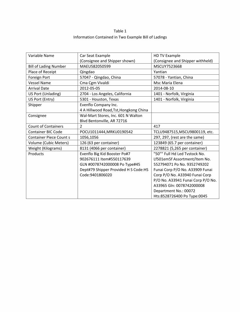
Table 1 

Information Contained in Two Example Bill of Ladings  

 

 

Variable Name  Car Seat Example (Consignee and Shipper shown) 

HD TV Example (Consignee and Shipper withheld) 

Bill of Lading Number  MAEU582050599  MSCUY7523668 

Place of Receipt  Qingdao  Yantian 

Foreign Port  57047 ‐ Qingdao, China  57078 ‐ Yantian, China 

Vessel Name  Cma Cgm Vivaldi  Msc Maria Elena 

Arrival Date  2012‐05‐05  2014‐08‐10 

US Port (Unlading)  2704 ‐ Los Angeles, California  1401 ‐ Norfolk, Virginia 

US Port (Entry)  5301 ‐ Houston, Texas  1401 ‐ Norfolk, Virginia 

Shipper  Evenflo Company Inc.  4 A Hillwood Road,Tst,Hongkong China 

 

Consignee  Wal‐Mart Stores, Inc. 601 N Walton Blvd Bentonville, AR 72716 

 

Count of Containers  2  417 

Container BIC Code  POCU1011444,MRKU0190542  TCLU9487515,MSCU9800119, etc. 

Container Piece Count s  1056,1056  297, 297, (rest are the same) 

Volume (Cubic Meters)  126 (63 per container)  123849 (65.7 per container) 

Weight (Kilograms)  8131 (4066 per container)  2278821 (5,265 per container) 

Products  Evenflo Big Kid Booster Po#7 902676111 Item#550117639  GLN #0078742000008 Po Type#45 Dept#79 Shipper Provided H S Code:HS Code:9401806020 

"50"" Full Hd Led Tvstock No. Lf501em5f Assortment/Item No. 552794071 Po No. 9352749202 Funai Corp P/O No. A33909 Funai Corp P/O No. A33940 Funai Corp P/O No. A33941 Funai Corp P/O No. A33965 Gln: 0078742000008 Department No.: 00072 Hts:8528726400 Po Type:0045 

 

   

Table 2 

Counts of Bills of Lading and Containers in Wal‐Mart Sample 

 

  Wal‐Mart Sample PIERS Published 

Aggregates  

 

Count of Shipments 

(1,000) 

Count Containers

(1,000)

Count Containers

(1,000 FEU*)

Sample Share Relative to PIERS 

(Percent) 

All Years  1,892  1,733 3,267** 53.1 

By Year     

2007  222  261 360 72.5 

2008  191  208 351*  59.4 

2009  165  160 342 46.8 

2010  179  167 348 48.0 

2011  179  154 355 43.4 

2012  186  149 360 41.4 

2013  238  198 366 54.2 

2014  259  212 388 54.7 

2015  273  224 398†  56.3 

 

*FEU is Forty Foot Equivalent.  PIERS reports units in TEU (Twenty Foot), so figures for PIERS are 

0.5×published figure. 

*The 2008 PIERS figure is based on interpolating 2007 and 2009.   †The 2015 PIERS figure is not yet available, and is estimated based on trend growth. 

   

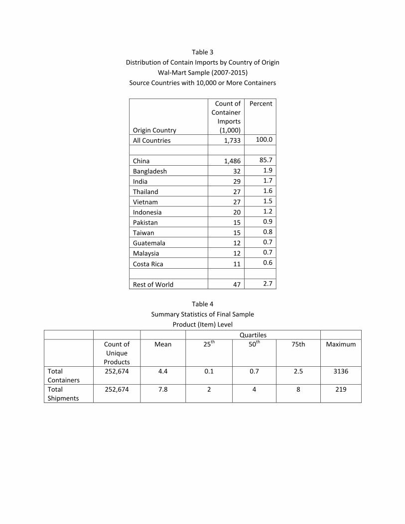
Table 3 

Distribution of Contain Imports by Country of Origin 

Wal‐Mart Sample (2007‐2015) 

Source Countries with 10,000 or More Containers 

 

Origin Country 

Count of Container Imports (1,000)

Percent

All Countries  1,733 100.0

 

China  1,486 85.7

Bangladesh  32 1.9

India  29 1.7

Thailand  27 1.6

Vietnam  27 1.5

Indonesia  20 1.2

Pakistan  15 0.9

Taiwan  15 0.8

Guatemala  12 0.7

Malaysia  12 0.7

Costa Rica  11 0.6

Rest of World  47 2.7

 

Table 4 

Summary Statistics of Final Sample 

Product (Item) Level 

      Quartiles   

  Count of Unique Products 

Mean  25th   50th  75th  Maximum 

Total Containers  

252,674  4.4  0.1  0.7  2.5  3136 

Total Shipments 

252,674  7.8  2  4  8  219 

 

   

Table 5 

Product 

Product Categories  Count of Unique Products 

Count of Shipments (1,000) 

Count of Containers (1,000) 

All Products  252,674 1,965 1,113

General Merchandise  135,768 1,460 836

Fashion  111,270 440 128

Sam’s Club  5,636 65 148

 

   

 

 

 

Table 6 

Distribution of Products by Number of DC Destinations 

General Merchansie and Fashion 

  General Merchandise  Fashion 

Count of Product Shipments 

Count Products  1 DC  2 DC  3 DC  4 DC  5 DC 

Count Products 1 DC 2 DC  3 DC  4 DC  5 DC 

1  23,569  1.00  36,044 1.00

2  13,192  0.35  0.65 21,457 0.80 0.20

3  11,253  0.12  0.17 0.71 12,020 0.68 0.15 0.16

4  14,490  0.04  0.09 0.11 0.75 10,044 0.49 0.24 0.09 0.18

5  15,318  0.02  0.04 0.09 0.10 0.75 7,518 0.50 0.13 0.08 0.12 0.17

6  3,971  0.05  0.10 0.25 0.33 0.27 5,265 0.51 0.17 0.08 0.12 0.12

7‐10  18,421  0.02  0.04 0.06 0.27 0.61 11,275 0.49 0.11 0.05 0.15 0.20

11‐20  17,245  0.02  0.02 0.02 0.15 0.79 6,439 0.49 0.14 0.02 0.10 0.26

21‐40  10,461  0.01  0.01 0.02 0.06 0.90 1,153 0.47 0.11 0.01 0.02 0.39

41 and above  7,848  0.00  0.00 0.01 0.02 0.97 55 0.13 0.02 0.00 0.07 0.78

 

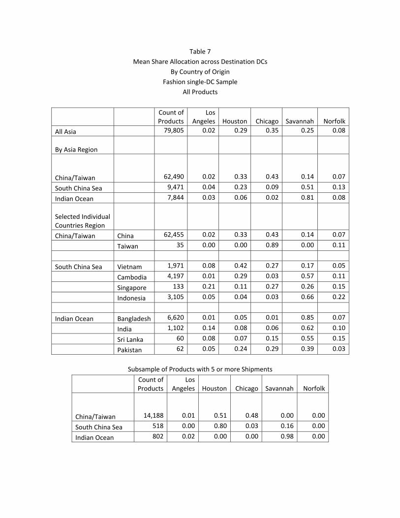
Table 7 

Mean Share Allocation across Destination DCs  

By Country of Origin 

Fashion single‐DC Sample 

All Products 

 

   Count of Products

Los Angeles Houston Chicago Savannah  Norfolk

All Asia  79,805 0.02 0.29 0.35 0.25  0.08

 By Asia Region 

China/Taiwan  62,490 0.02 0.33 0.43 0.14  0.07

South China Sea    9,471 0.04 0.23 0.09 0.51  0.13

Indian Ocean  7,844 0.03 0.06 0.02 0.81  0.08

 Selected Individual Countries Region     

China/Taiwan  China  62,455 0.02 0.33 0.43 0.14  0.07

Taiwan  35 0.00 0.00 0.89 0.00  0.11

     

South China Sea  Vietnam  1,971 0.08 0.42 0.27 0.17  0.05

  Cambodia  4,197 0.01 0.29 0.03 0.57  0.11

  Singapore  133 0.21 0.11 0.27 0.26  0.15

Indonesia  3,105 0.05 0.04 0.03 0.66  0.22

     

Indian Ocean  Bangladesh  6,620 0.01 0.05 0.01 0.85  0.07

India  1,102 0.14 0.08 0.06 0.62  0.10

  Sri Lanka  60 0.08 0.07 0.15 0.55  0.15

Pakistan  62 0.05 0.24 0.29 0.39  0.03

 

Subsample of Products with 5 or more Shipments 

 Count of Products

Los Angeles Houston Chicago Savannah  Norfolk

China/Taiwan  14,188 0.01 0.51 0.48 0.00  0.00

South China Sea  518 0.00 0.80 0.03 0.16  0.00

Indian Ocean  802 0.02 0.00 0.00 0.98  0.00

 

   

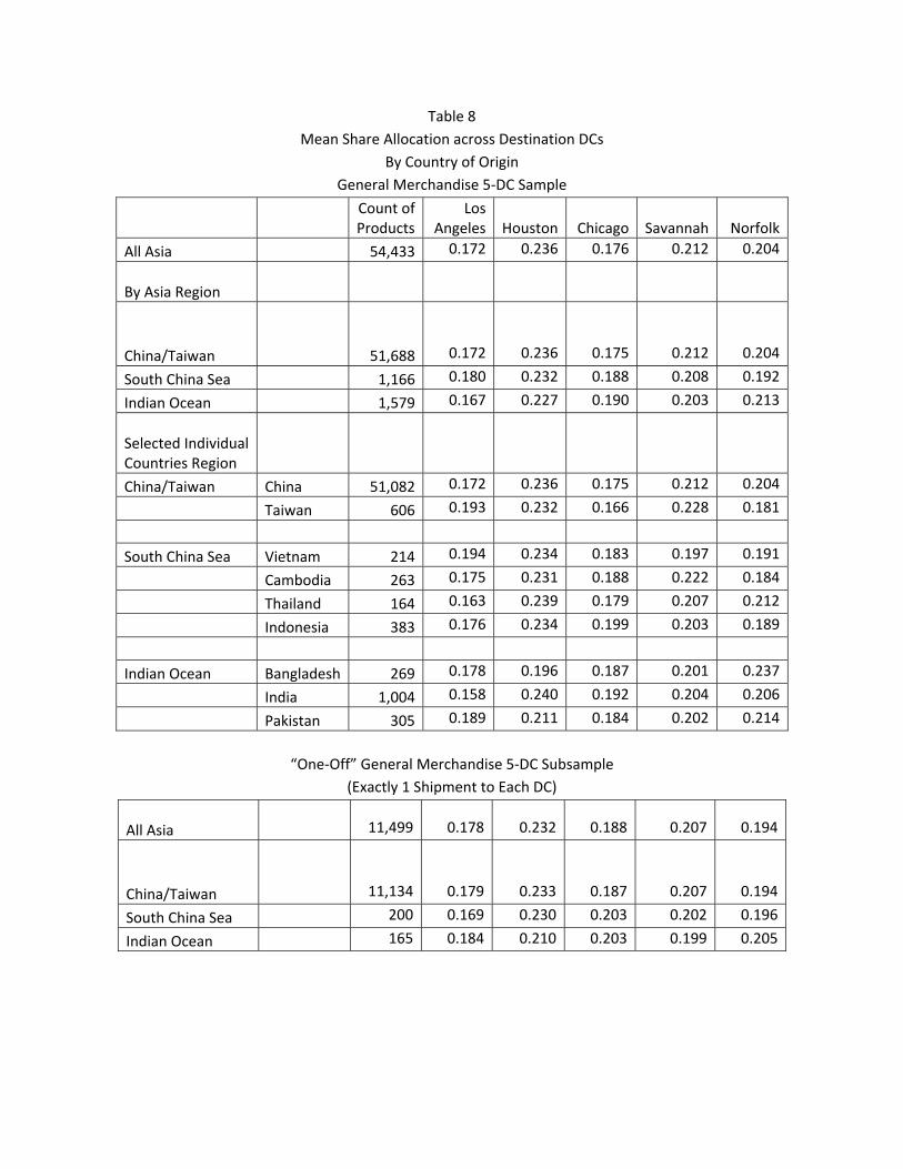
Table 8 

Mean Share Allocation across Destination DCs  

By Country of Origin 

General Merchandise 5‐DC Sample 

   Count of Products

Los Angeles Houston Chicago Savannah  Norfolk

All Asia  54,433 0.172 0.236 0.176 0.212  0.204

 By Asia Region 

China/Taiwan  51,688 0.172 0.236 0.175 0.212  0.204

South China Sea    1,166 0.180 0.232 0.188 0.208  0.192

Indian Ocean  1,579 0.167 0.227 0.190 0.203  0.213

 Selected Individual Countries Region     

China/Taiwan  China  51,082 0.172 0.236 0.175 0.212  0.204

Taiwan  606 0.193 0.232 0.166 0.228  0.181

     

South China Sea  Vietnam  214 0.194 0.234 0.183 0.197  0.191

  Cambodia  263 0.175 0.231 0.188 0.222  0.184

  Thailand  164 0.163 0.239 0.179 0.207  0.212

Indonesia  383 0.176 0.234 0.199 0.203  0.189

     

Indian Ocean  Bangladesh  269 0.178 0.196 0.187 0.201  0.237

India  1,004 0.158 0.240 0.192 0.204  0.206

Pakistan  305 0.189 0.211 0.184 0.202  0.214

 

“One‐Off” General Merchandise 5‐DC Subsample  

(Exactly 1 Shipment to Each DC) 

 All Asia  11,499 0.178 0.232 0.188 0.207  0.194

China/Taiwan  11,134 0.179 0.233 0.187 0.207  0.194

South China Sea    200 0.169 0.230 0.203 0.202  0.196

Indian Ocean  165 0.184 0.210 0.203 0.199  0.205

 

   

 

 

Table 9 Port Choice Given Destination DC 

Footwear/Clothing 1‐DC Sample 

 

  Destination is Houston DC  Destination is Chicago DC 

 

Count 

Shipment 

Los 

Angeles 

Port 

Share

Houston 

Port 

Share

Los 

Angeles 

Port 

Share

Seattle 

Port 

Share 

New 

York 

Port 

Share

China/Taiwan  87,862  0.42 0.58 102,566 0.00 1.00  0.00

South China Sea  6,074  0.62 0.38 1,561 0.10 0.90  0.00

Indian Ocean  496  0.10 0.90 205 0.58 0.20  0.22

 

General Merchandise 5‐DC Sample 

 

  Destination is Houston DC  Destination is Chicago DC 

 

Count 

Shipments 

Los 

Angeles 

Port 

Share

Houston 

Port 

Share

Los 

Angels 

Port 

Share

Seattle 

Port 

Share 

New 

York 

Port 

Share

China/Taiwan  223,120  0.16 0.84 197,069 0.57 0.42  0.00

South China Sea  4,250  0.57 0.43 3,566 0.80 0.20  0.00

Indian Ocean  8,043  0.08 0.92 8,498 0.17 0.02  0.81

 

   

 

Table 10 

Port Choice Estimates 

Value of time  σε XNY,CHI ‐ XLA,CHI  XSEA,CHI ‐ XLA,CHI  XHOU,HOU ‐ XLA,HOU 

All items  $18 113 ‐273.4 ‐58.2  ‐852.2

General Merchandise  $12 96 ‐256.1 1.1  ‐813.8

Fashion (Footwear and apparel)  $92 357 ‐379.2 ‐889.2  ‐1370.4

 

 

Table 11 

DC Choice Estimates, General Merchandise 

   ση= σε ση= 0.5σε ση= 2σε

YCHI  141 165 124 

YNOR  ‐628 ‐614 ‐625 

YSAV  ‐918 ‐946 ‐860 

YLAX  0 0 0 

YHOU  ‐86 ‐87 ‐67 

 

   

Table 12  

Estimated Cost Per Container 

By Origination and by Distribution System 

(All relative to Origination from China with the 5‐DC System,  

and Cost to Los Angeles Normalized to Zero) 

 

Country  5‐DC 

3‐DC (exclude CHI and HOU) 

1‐DC CHI 

1‐DC HOU 

1‐DC SAV 

1 DC NOR 

I‐DC LAX 

China  0 228 741 525 508  748 974

Taiwan  80 331 741 615 645  885 974

 South China Sea: 

 

Vietnam  47 287 741 581 586  826 974

Cambodia  33 247 749 614 535  771 974

Singapore  5 210 749 587 486  722 974

Indonesia  73 304 749 645 611  847 974

 Indian Ocean: 

 

Bangladesh  ‐68 112 747 517 336  616 974

India  ‐367 ‐204 645 94 ‐60  182 974

Sri Lanka  ‐456 ‐294 575 2 ‐199  81 974

Pakistan  ‐601 ‐416 411 ‐174 ‐333  ‐103 974

 

   

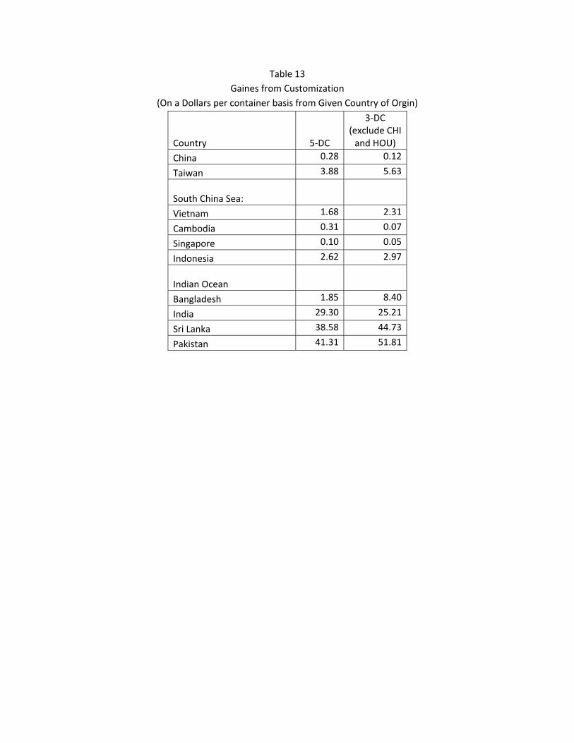
Table 13  

Gaines from Customization 

(On a Dollars per container basis from Given Country of Orgin) 

Country  5‐DC 

3‐DC (exclude CHI and HOU) 

China  0.28 0.12

Taiwan  3.88 5.63

 South China Sea: 

Vietnam  1.68 2.31

Cambodia  0.31 0.07

Singapore  0.10 0.05

Indonesia  2.62 2.97

 Indian Ocean 

Bangladesh  1.85 8.40

India  29.30 25.21

Sri Lanka  38.58 44.73

Pakistan  41.31 51.81

 

   

 

 

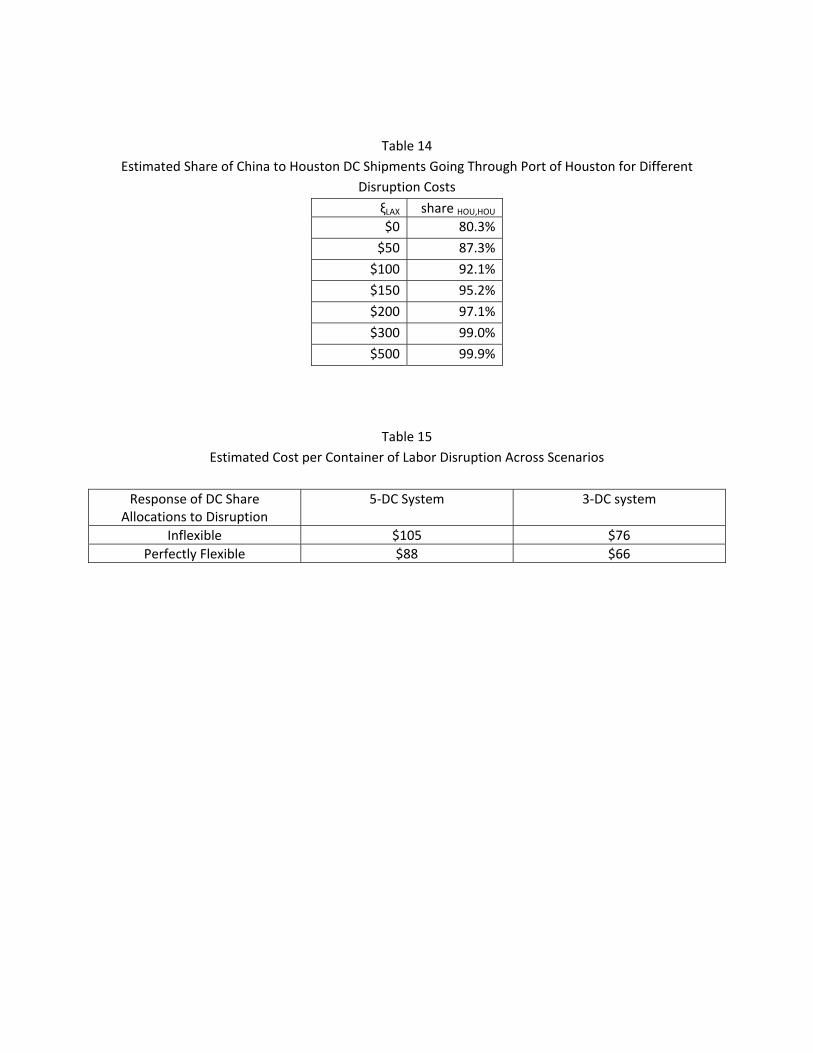
Table 14 

Estimated Share of China to Houston DC Shipments Going Through Port of Houston for Different 

Disruption Costs 

ξLAX share HOU,HOU$0  80.3%

$50  87.3%

$100  92.1%

$150  95.2%

$200  97.1%

$300  99.0%

$500  99.9%

 

 

 

Table 15 

Estimated Cost per Container of Labor Disruption Across Scenarios 

 

Response of DC Share Allocations to Disruption 

5‐DC System  3‐DC system 

Inflexible  $105   $76  

Perfectly Flexible  $88   $66  

 

 

   

 

 

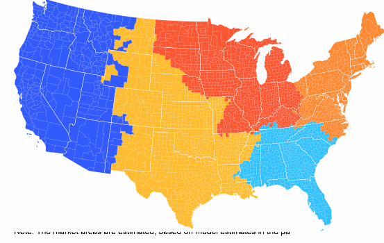
Figure 2 

Voyage Duration and Port Choice During West Coast Port Slowdown 

Median Time from Shenzhen or Shanghai to Los Angeles (by week of departure) 

Share of Containers Destined for Houston Going Through Los Angeles 

  

 

   

0.00

0.10

0.20

0.30

0.40

0.50

0.60

0.70

0.80

0

5

10

15

20

25

30

35

40

12/15/2013

1/15/2014

2/15/2014

3/15/2014

4/15/2014

5/15/2014

6/15/2014

7/15/2014

8/15/2014

9/15/2014

10/15/2014

11/15/2014

12/15/2014

1/15/2015

2/15/2015

3/15/2015

4/15/2015

5/15/2015

6/15/2015

7/15/2015

8/15/2015

9/15/2015

10/15/2015

11/15/2015

days

LA share

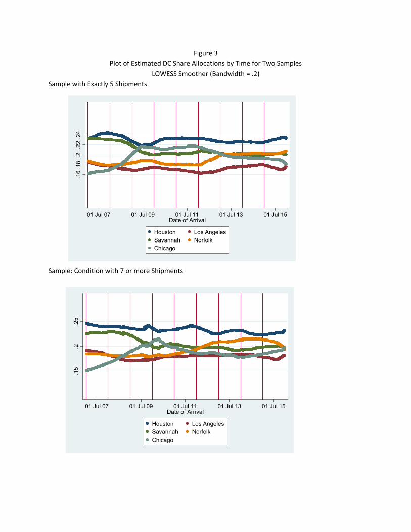
Figure 3 

Plot of Estimated DC Share Allocations by Time for Two Samples 

LOWESS Smoother (Bandwidth = .2) 

Sample with Exactly 5 Shipments 

 

 

 

 

 

 

 

 

 

 

 

 

 

 

 

 

 

Sample: Condition with 7 or more Shipments  

.15

.2.2

5

01 Jul 07 01 Jul 09 01 Jul 11 01 Jul 13 01 Jul 15Date of Arrival

Houston Los AngelesSavannah NorfolkChicago

.16

.18

.2.2

2.2

4

01 Jul 07 01 Jul 09 01 Jul 11 01 Jul 13 01 Jul 15Date of Arrival

Houston Los AngelesSavannah NorfolkChicago