estimates of state and metropolitan price parities for consumption
TRANSCRIPT

October 29th, 2008
Estimates of State and Metropolitan Price Parities for Consumption Goods and Services in the United States, 2005
Bettina H. Aten ∗
Abstract
Price indexes are commonly used in time-to-time economic series to adjust for changes in price levels across years. This paper estimates price parities within the U.S., defined as an adjustment for differences in price levels across geographic areas at one point in time. The term parity is more frequently used in international comparisons, where purchasing power parities (PPPs) are divided by the exchange rate to denote differences in price levels across countries. The method described here for calculating regional PPPs is based on micro-level price data from the Consumer Price Index of the Bureau of Labor Statistics and on the American Community Survey of the Census Bureau. It uses a Bayesian spatial smoothing approach to obtain individual county price levels that are aggregated to regional price parities (RPPs) for 363 metropolitan areas and 51 states in the United States. An example of their relevance is given by comparing the Personal Income and Gross Domestic Product estimates produced by the Bureau of Economic Analysis for the year 2005 at national prices and at regional price parities.
Introduction This paper develops exploratory estimates of the spatial price differences for consumption goods and services at the U.S. state and metropolitan area level for 2005. Spatial (place-to-place) price differences are important to regional and other sub-national accounting frameworks as they make possible comparisons of economic data that are adjusted for geographic differences in price levels. In international comparisons, these adjustments are termed purchasing power parities (PPP); when divided by exchange rates they are called national price levels. In areas with a common currency like the Euro, the exchange rates are the same and the PPP becomes the price level. Just as there are differences in price levels between European Union member countries, there are significant differences in the purchasing power of a currency across diverse areas of the United States, for example between metropolitan New York compared to rural South Dakota. We use the term Regional Price Parity (RPPs) to label these sub-national estimates of PPPs. The RPPs can be used to adjust consumption-related ∗ Bettina H. Aten is an economist in the Regional Economics Directorate, Bureau of Economic Analysis. The results presented here are the responsibility of the author and not of the Bureau of Economic Analysis. Email: [email protected].
1 of 28

statistics, such as per capita incomes, expenditures and output, providing users with a more accurate picture of regional economic differences at one point in time. See for example Bernstein et al [2000], Johnson et al [2001], and Jollife [2006]. The RPPs are built up in this paper from two main data sets. The first is the principal source of consumer price information in the United States, the Bureau of Labor Statistics Consumer Price Index (CPI) for 38 metropolitan and urban areas, which is of course used for time-to-time indexes. Aten (2006) presented regional price parity estimates for 2003 and 2004 for these 38 areas, which cover 87% of the population but only about 15% of U.S. counties. In addition, some states are not covered at all by the CPI. The second source of information is the county level monthly median costs for owners and renters from the 2005 American Community Survey (ACS) of the U.S. Census Bureau, adjusted for quality differences. This adjustment is described in the next section. Henceforth, the housing costs denote the average of these costs – that is, the geometric mean1 of the median selected monthly owner costs (with and without mortgages) and median gross rents2. The sub-national price level estimates presented here are generated using Bayesian inference and a two-stage approach that bridges the results in the areas sampled by the CPI price surveys to the remaining non-sampled areas covered by the Census.
Methodology and Data
BLS data: Price Parities The background methodology and data on estimating place-to-place price parities for the 38 metropolitan and urban areas in the CPI for one year price levels is detailed in Aten [2005, 2006]. The estimation of these parities begins with over a million price quotes and detailed hedonic regressions for over two hundred consumption goods and services items. These items range from new automobiles to haircuts, and include consumption expenditures on shelter, or rents. The CPI rents estimated within the BLS framework are different from the ACS and Census housing costs in that the former uses owner-equivalent rents3 rather than actual owner-costs.
1 The ACS tables (Tables B25088 and B25064) provide the number of owner-occupied versus rental housing units. Housing costs are calculated as the weighted geometric mean of the ownership costs and gross rents, where the weights equal the proportion of owned and rented housing units in each county. 2“Selected monthly owner costs are the sum of payments for mortgages, deeds of trust, contracts to purchase, or similar debts on the property; real estate taxes: fire, hazard, and flood insurance on the property; utilities (electric, gas, water, and sewer); and fuels (oil, coal, kerosene, wood, and so on). It also includes, where appropriate, the monthly condominium fee for condominiums and mobile home costs”, “ Gross rent is the contract rent plus the estimated average monthly cost of utilities and fuels if these are paid by the renter”, page 64: http://www.census.gov/acs/www/SBasics/congress_toolkit/Housing%20Fact%20Sheets.pdf 3 http://www.bls.gov/cpi/cpifact6.htm
2 of 28

The hedonic regressions take into account item characteristics, such as unit size and packaging, as well as the location and type of outlet where the item is sold, and uses probability sampling quotes as weights4. The resulting item price levels are then aggregated into major categories, such as Food and Beverages, Transportation, and Housing5, and up to an overall RPP for consumption. The aggregation method follows the Rao-system of multilateral price comparisons (Rao [2005]) and uses the itemized expenditures of each area as weights (see Appendix Table A1 in Aten [2006] for a list of all counties comprising these areas). One shortcoming of this background work is its limited geographical coverage, albeit representing the great majority of the country’s population. This is because the CPI survey is designed as a probability sample to estimate price changes over time, not price differences across locations6. More disaggregated item calculations or more extensive geographical coverage would require a redesign of the CPI survey, something that is not feasible in the short run.
Census data: Housing Costs The data on housing costs are taken from the Census Bureau. A previous version of this paper (Aten, 2007) used Census 2000 data, moving back the estimated price levels from 2003 to 2000 by the urban and non-urban CPI changes7. This paper instead uses 2005 prices and the more recent 2005 American Community Survey (ACS). The 2005 ACS includes all counties with a population of 65,000 or more, a total of about 780 counties covering 82 percent of the nation’s population. It also includes the proportion of owners and renters in each county, as well as median gross rents and selected monthly owner costs8. In addition, an adjustment is made for the ‘quality’ of the rental and owned housing stock. Quality-adjustment in this context means taking into account various characteristics of the housing observations, namely number of rooms, bathrooms, age, kitchen and plumbing facilities, and the type of unit – whether it is a detached or attached house, a small or a large apartment building for example, in addition to the mortgage status (for owners). 4 Since the author anticipates estimating the 38 interarea price levels annually, the results for 2005 onward will be available as tables rather than published papers. Effort is underway to make them available for downloading at the BLS website as well as from BEA. 5 Housing items in the CPI also include Rents. Rents in the BLS are distinct from Rents in the Census, as the former imputes the owner-equivalent rents using utility costs and other adjustments (for a more detailed description, see Aten [2006]). 6The individual price quotes of the CPI are identified by location (zip code in most cases), but full coverage of all items exist only when aggregated to the 38 metro and urban areas. This is because the probability quote weights for the samples as well as the detailed expenditure weights by item are only available for the 38 areas. 7 Aten (2006) compares an extrapolation of 2003 to 2004 versus a direct estimate for the year 2004 and finds that there are minor differences when an aggregate CPI rate is used as the deflator, but negligible differences with a detailed item-level CPI deflator. 8 2005, 2006 ACS FactFinder, subject tables B25088 and B25064 and an earlier footnote (Footnote 2) .
3 of 28
These detailed characteristics are only available at the Public Use Microdata Sample (PUMS) level, and not identifiable at the county level, so a quality adjustment factor can only be obtained at the next aggregate level, the state level9. The factor is the ratio of the average value of quality-adjusted housing to unadjusted housing using a separate hedonic regression for renters versus owners with the characteristics listed above. The median gross rent and the monthly owner cost in each county are multiplied by the corresponding quality adjustment factors, and the results averaged in proportion to the number of owners and renters. The result is termed housing costs for simplicity. The 2005 housing costs for counties not in the ACS were computed in the following way. Their 2000 Census housing costs were moved to 2005 using the population weighted geometric mean of the ACS counties for each state. In other words, the change in median housing costs for these smaller (less than 65,000 population) counties was assumed to reflect the average change across the larger counties within each state, weighted by their populations. Henceforth Census housing costs will denote these quality adjusted weighted averages of renters and owners that include both ACS and smaller counties10.
Method The starting point of the estimation procedure is the set of 38 price levels obtained directly from price quotes and hedonic regressions using the BLS data. These price levels are strongly related to the housing costs as shown in Figure 1. The price level - rent relationship across these areas is assumed to hold within the areas, so that using the estimated coefficients from Equation (1), the price levels for the 425 counties that make up these 38 areas can be obtained11. They are then adjusted so that their population weighted means equal the 38 original area means. 9 The ACS PUMS housing records for 2005 consist of over 280,000 rent observations and 855,000 owner observations, and are described in http://www.census.gov/acs/www/Products/PUMS/ 10 Observations in the Census data follow several designations: county is the lowest aggregation for many states, but for others there are Places and MCDs within a county FIPS code. For example, there are five townships in Maine that are part of York County, which in turn is one of the ten counties in the A103 Boston metropolitan area. Connecticut, Massachusetts, Vermont and New Hampshire also have several towns or cities within a county code. Unless otherwise noted, the subdivisions are aggregated to the county level. In the case of housing costs, this is the weighted geometric mean of the Places or MCDs within each county. 11 A few counties span more than one CPI area, primarily when the county is comprised of townships. In these cases, the FIPS code of the county was assigned to one area only, based on the size of the sample and/or the population that it covered. They are the following:
Litchfield, CT to area A110 (New York Suburbs) Middlesex, CT to area X100 (Northeast B region) Windham, CT to area X100 (Northeast B region) Hampden, MA to area X100 (Northeast B region)
Eight towns within Litchfield are in the A110 area and five are in the X100 region but the ones in the A110 area account for two thirds of the population. Seven out of eight towns in Middlesex are in the X100 area, with 79% of the population. In Windham, only Thompson town with 11% of the population is in the A103 Boston with the rest in the X100 area, and similarly in Hampden, only Holland town with less than one percent of the population is in A103, with the remainder in the X100 Northeast B area.
4 of 28

A second set of parameters are then estimated using Equation (2). The 425 county housing costs and also their relative locations are modeled explicitly, resulting in a set of spatially smoothed estimates. Both equations use a Bayesian framework, allowing the variances of the error terms to be non-constant. In addition, Equation (2) is written as a spatial model with missing dependent variables (the price levels to be estimated for the remaining counties), and an adjustment is made to include the housing costs of the missing observations as well as their relative location. These will be discussed further below. There are two main issues that arise from this methodology. The first is a change-of-scale problem - from the 38 BLS areas to the 425 counties that comprise them, and the second one a change-of-sample problem - from the 425 counties that belong the BLS sample to the remaining counties. The change-of-scale problem arises partly because some of the 38 areas cross state lines and represent larger regions, while others refer to single counties. For example, the District of Columbia is only one of 26 counties in the Greater Washington metropolitan area as defined in the CPI, but it is also a quasi state, or at least, for many purposes, a separate entity from the states of Virginia or Maryland. Los Angeles is one county and one BLS area by itself, but only one of 58 counties in the state of California. The BLS area termed South B (medium and small urban areas in the South Region), is made up of 84 smaller units, scattered across states such as Georgia, Tennessee, and South Carolina. Combining and using these disparate spatial units, as well as issues related to scale, classification inconsistencies and sampling coverage have been discussed in the spatial econometric (Anselin [2002]), and geostatistical literature by Goodchild, Anselin and Deichmann [1993], Gotway and Young [2002], Baneerje and Gelfand [2004], and Anselin and Gallo [2006]. Holt, Trammer, Stell and Wrigley [1996] and Huang and Cressie [1997] have proposed some adjustments to deal with the differences between aggregation levels. The approach used here hopes to mitigate, rather than resolve some of the problems associated with changes of scale and spatial aggregation, but is by necessity data-driven and constrained by the sampling coverage. The second main issue in making inferences for areas not sampled by the BLS CPI is by construction: the survey design systematically excludes the smaller, less densely populated counties which have lower volumes of expenditures. This means that direct inferences from the sampled areas of the CPI to the non-sampled areas would be misleading because the distribution of expenditures and prices are also likely to be systematically different12.
12 The unweighted average housing costs for the 425 counties is $1,003 while for all other counties it is $594. The two-sample equality of means t-test statistic is 25.99 (p<0.0001).
5 of 28
One approach that has proven successful in predicting sampled versus non-sampled observations is the use of a best linear unbiased predictor (BLUP) for missing dependent variables (Goldberger [1962], Cressie [1993], Kelejian and Prucha [2004]). The spatial econometric equivalent of the BLUP is termed an endogenous spatial smoothing approach given in LeSage and Pace [2004, 2007] and is adopted here. In the final stage, the predicted county price level estimates are aggregated to the state and the metropolitan area level, weighted by the total value of wage and salary disbursements in each county. These weighted aggregate price levels are the Regional Price Parities or RPPs. Total wage and salary disbursements include supplements, such as employer contributions to social security and are termed Compensation of Employees. Compensation of Employees enters into the calculation of GDP and Personal Income by state and metropolitan areas at BEA13. Ideally, one would use the consumption expenditures of individuals rather than the compensation of employees to weight the consumption-based price levels, but expenditures are not available at a detailed geographic level, whereas compensation data are. Another argument for using compensation is that it is a major component of total product on the income side of GDP accounting, just as expenditures generally account for the largest proportion of GDP from the expenditure side. To highlight the use of RPPs, estimates of income and product at national prices versus estimates adjusted for regional price differences are presented. They are calculated by adjusting the Compensation of Employees total in Personal Income and GDP by the RPP, then adding the unadjusted remainder. This unadjusted remainder includes such components as taxes, transfers, dividends and interest, and are explained in more detail in Lenze (2007) and Panek, Baumgardner and McCormick (2007).
Results
Figure 1 plots the relationships between the original price levels and the housing costs for 2005.
13 County level Compensation of Employees are available from the BEA website, as are Personal Income and GDP totals by state and metropolitan areas. See http://bea.gov/regional/index.htm for the data and methodology.
6 of 28
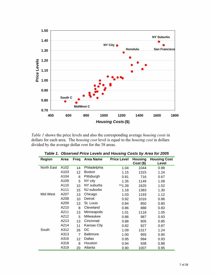
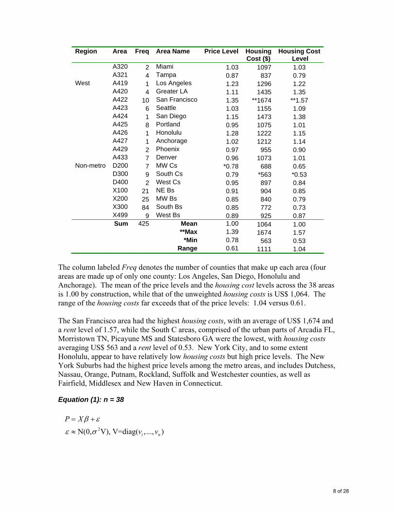
Table 1 shows the price levels and also the corresponding average housing costs in dollars for each area. The housing cost level is equal to the housing cost in dollars divided by the average dollar rent for the 38 areas.
Table 1. Observed Price Levels and Housing Costs by Area for 2005 Region Area Freq Area Name Price Level Housing
Cost ($) Housing Cost
Level North East A102 14 Philadelphia 1.04 1044 0.98 A103 12 Boston 1.15 1315 1.24 A104 6 Pittsburgh 0.81 716 0.67 A109 5 NY city 1.35 1149 1.08 A110 10 NY suburbs **1.39 1620 1.52 A111 15 NJ suburbs 1.18 1383 1.30 Mid West A207 13 Chicago 1.03 1193 1.12 A208 10 Detroit 0.92 1016 0.96 A209 13 St. Louis 0.84 850 0.80 A210 8 Cleveland 0.86 888 0.83 A211 13 Minneapolis 1.01 1118 1.05 A212 5 Milwaukee 0.86 987 0.93 A213 13 Cincinnati 0.88 905 0.85 A214 11 Kansas City 0.82 927 0.87 South A312 26 DC 1.09 1317 1.24 A313 7 Baltimore 1.00 955 0.90 A316 12 Dallas 0.95 994 0.93 A318 8 Houston 0.94 938 0.88 A319 20 Atlanta 0.90 1007 0.95
0.70
0.80
0.90
1.00
1.10
1.20
1.30
1.40
1.50
400 600 800 1000 1200 1400 1600 1800
Housing Costs ($)
Pric
e Le
vels
South C
MidWest C
NY City
NY Suburbs
San FranciscoHonolulu
7 of 28
Region Area Freq Area Name Price Level Housing Cost ($)
Housing Cost Level
A320 2 Miami 1.03 1097 1.03 A321 4 Tampa 0.87 837 0.79 West A419 1 Los Angeles 1.23 1296 1.22 A420 4 Greater LA 1.11 1435 1.35 A422 10 San Francisco 1.35 **1674 **1.57 A423 6 Seattle 1.03 1155 1.09 A424 1 San Diego 1.15 1473 1.38 A425 8 Portland 0.95 1075 1.01 A426 1 Honolulu 1.28 1222 1.15 A427 1 Anchorage 1.02 1212 1.14 A429 2 Phoenix 0.97 955 0.90 A433 7 Denver 0.96 1073 1.01 Non-metro D200 7 MW Cs *0.78 688 0.65 D300 9 South Cs 0.79 *563 *0.53 D400 2 West Cs 0.95 897 0.84 X100 21 NE Bs 0.91 904 0.85 X200 25 MW Bs 0.85 840 0.79 X300 84 South Bs 0.85 772 0.73 X499 9 West Bs 0.89 925 0.87
Sum 425 Mean 1.00 1064 1.00 **Max 1.39 1674 1.57 *Min 0.78 563 0.53 Range 0.61 1111 1.04
The column labeled Freq denotes the number of counties that make up each area (four areas are made up of only one county: Los Angeles, San Diego, Honolulu and Anchorage). The mean of the price levels and the housing cost levels across the 38 areas is 1.00 by construction, while that of the unweighted housing costs is US$ 1,064. The range of the housing costs far exceeds that of the price levels: 1.04 versus 0.61. The San Francisco area had the highest housing costs, with an average of US$ 1,674 and a rent level of 1.57, while the South C areas, comprised of the urban parts of Arcadia FL, Morristown TN, Picayune MS and Statesboro GA were the lowest, with housing costs averaging US$ 563 and a rent level of 0.53. New York City, and to some extent Honolulu, appear to have relatively low housing costs but high price levels. The New York Suburbs had the highest price levels among the metro areas, and includes Dutchess, Nassau, Orange, Putnam, Rockland, Suffolk and Westchester counties, as well as Fairfield, Middlesex and New Haven in Connecticut.
Equation (1): n = 38
2
N(0, V), V=diag( ,..., )
i n
P Xv v
β ε
ε σ
= +
≈
8 of 28
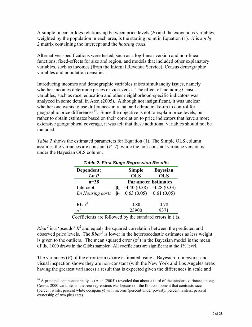
A simple linear-in-logs relationship between price levels (P) and the exogenous variables, weighted by the population in each area, is the starting point in Equation (1). X is a n by 2 matrix containing the intercept and the housing costs. Alternatives specifications were tested, such as a log-linear version and non-linear functions, fixed-effects for size and region, and models that included other explanatory variables, such as incomes (from the Internal Revenue Service), Census demographic variables and population densities. Introducing incomes and demographic variables raises simultaneity issues, namely whether incomes determine prices or vice-versa. The effect of including Census variables, such as race, education and other neighborhood-specific indicators was analyzed in some detail in Aten (2005). Although not insignificant, it was unclear whether one wants to use differences in racial and ethnic make-up to control for geographic price differences14. Since the objective is not to explain price levels, but rather to obtain estimates based on their correlation to price indicators that have a more extensive geographical coverage, it was felt that these additional variables should not be included. Table 2 shows the estimated parameters for Equation (1). The Simple OLS column assumes the variances are constant (V=I), while the non-constant variance version is under the Bayesian OLS column.
Table 2. First Stage Regression Results Dependent:
Ln P Simple
OLS Bayesian
OLS n=38 Parameter Estimates
Intercept β1 -4.40 (0.38) -4.28 (0.33)Ln Housing costs β2 0.63 (0.05) 0.61 (0.05)
Rbar2 0.80 0.78 σ2 23900 9371
Coefficients are followed by the standard errors in ( )s. Rbar2 is a ‘pseudo’ R2 and equals the squared correlation between the predicted and observed price levels. The Rbar2 is lower in the heteroscedastic estimates as less weight is given to the outliers. The mean squared error (σ2) in the Bayesian model is the mean of the 1000 draws in the Gibbs sampler. All coefficients are significant at the 1% level. The variances (V) of the error term (ε) are estimated using a Bayesian framework, and visual inspection shows they are non-constant (with the New York and Los Angeles areas having the greatest variances) a result that is expected given the differences in scale and 14 A principal component analysis (Aten [2005]) revealed that about a third of the standard variance among Census 2000 variables in the rent regressions was because of the first component that contrasts race (percent white, percent white occupancy) with income (percent under poverty, percent renters, percent ownership of two plus cars).
9 of 28
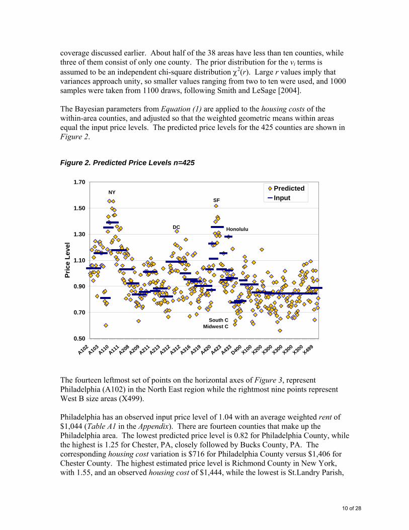
coverage discussed earlier. About half of the 38 areas have less than ten counties, while three of them consist of only one county. The prior distribution for the vi terms is assumed to be an independent chi-square distribution χ2(r). Large r values imply that variances approach unity, so smaller values ranging from two to ten were used, and 1000 samples were taken from 1100 draws, following Smith and LeSage [2004]. The Bayesian parameters from Equation (1) are applied to the housing costs of the within-area counties, and adjusted so that the weighted geometric means within areas equal the input price levels. The predicted price levels for the 425 counties are shown in Figure 2.
Figure 2. Predicted Price Levels n=425
The fourteen leftmost set of points on the horizontal axes of Figure 3, represent Philadelphia (A102) in the North East region while the rightmost nine points represent West B size areas (X499). Philadelphia has an observed input price level of 1.04 with an average weighted rent of $1,044 (Table A1 in the Appendix). There are fourteen counties that make up the Philadelphia area. The lowest predicted price level is 0.82 for Philadelphia County, while the highest is 1.25 for Chester, PA, closely followed by Bucks County, PA. The corresponding housing cost variation is $716 for Philadelphia County versus $1,406 for Chester County. The highest estimated price level is Richmond County in New York, with 1.55, and an observed housing cost of $1,444, while the lowest is St.Landry Parish,
0.50
0.70
0.90
1.10
1.30
1.50
1.70
A102A103
A110A111
A208A209
A211A213
A312A312
A316A319
A420A423
A433D400
X100X20
0X30
0X300
X300X30
0X49
9
Pric
e Le
vel
PredictedInput
Honolulu
NYSF
South CMidwest C
DC
10 of 28

Louisiana, with a price level of 0.56 and housing costs averaging $397. The highest housing cost across all 425 counties was in Marin County, CA, at $2016 and its estimated price level was 1.52.
Equation (2): Spatial Bayesian Model (n=425 )
2
N(0, V), V=diag( ,..., )
i n
P WP Xv v
λ β ε
ε σ
= + +
≈
Equation (2) is similar to Equation (1) but adds a n by n spatial weight matrix W. The X matrix also includes the spatial weight matrix and is analogous to a spatial Durbin variable15: X is an n by 3 matrix with the 3 columns equal to an intercept, housing costs, and W*housing costs. As in Equation (1), the prior distribution for the vi terms is assumed to be an independent chi-square distribution χ2(r) and is obtained using a Gibbs sampler. The matrix W is a non-negative spatial weight matrix with zeros on the diagonal and non-zero entries reflecting the spatial proximity of one county to another. A non-zero element Wik defines i and k as geographical neighbors. The term neighbor in this context may range from nearest neighbors, to contiguity, to inverse distance matrix definitions of neighbors. For example, a first-order nearest neighbor matrix will have ones in the row and columns corresponding to observations that are closest to each other geographically, and zero otherwise16. Inverse distance matrices will have entries in all the elements (except the main diagonal) indicating the inverse of the distance between the observations. The contiguity matrix is defined using a Delaunay triangulation17, with observations having from three to twelve neighbors. This is the matrix chosen for this paper. See Aten [2007] for an analysis of the sensitivity of different spatial weight matrices to the final estimated price levels.
Table 3. Second Stage Regression Results Dependent:
Ln P Spatial Bayesian
n=425 Parameter Estimates
W*lnP λ 0.20 (.02)Intercept β1 -3.83 (.07)Ln Housing costs β2 0.55 (.01)
15 For a review of the estimation of spatial econometric models, including their specification, see for example, Anselin [1988, 2002, 2004], Getis et al [2004], LeSage et al [2004]. 16 Other metrics, such as trade or commuting flows may be used in the W matrix, but distance is an easy to compute variable that is clearly exogenous, and has been shown to be correlated to price levels in other studies (Aten [1996, 1997]). 17 Delaunay triangles (the dual of a Voronoi diagram, also know as Thiessen polygons) returns a set of triangles such that no data points are contained in any triangle's circumcircle. The contiguity matrix is the adjacency matrix derived from this triangulation.
11 of 28

Dependent: Ln P
Spatial Bayesian
W*Ln Housing costs
β3 -0.002 (.0009)
Rbar2 0.84 σ2 289
Coefficients are followed by the standard errors in ( ). Following the notation in Pace and LeSage [2007], the variables in Equation (2) are partitioned into the set of observations for the BLS counties (labeled with the subscript 1) and the remaining counties (subscript 2). The X matrix equals [X1 X2] and P = [P1 P2], with n=n1 + n2. Similarly the spatial weight matrix W is partitioned into W11, W12, W21 and W22. This means that W11, the weight matrix for the counties in the BLS, reflects their contiguity within the larger set of all U.S. counties, not as a separate set of spatial locations18. The partitions are shown in Equation (3).
Equation (3): Partitioned n (n1 = 425, n2 = 2713)
1 11 12 1 1 1
2 21 22 2 2 2
p W W p Xp W W p X
ελ β
ε⎛ ⎞ ⎛ ⎞⎛ ⎞ ⎛ ⎞ ⎛ ⎞
= + +⎜ ⎟ ⎜ ⎟⎜ ⎟ ⎜ ⎟ ⎜ ⎟⎝ ⎠ ⎝ ⎠⎝ ⎠ ⎝ ⎠ ⎝ ⎠
P2 are the unobserved, missing price levels for the counties not in the BLS sample, that is, the ones to be predicted, while X2, the housing costs and spatially lagged (W*housing costs) housing costs for these counties are observed. We use the estimated βs and λ from Table 3 to obtain an exogenous prediction E(p2) , shown in Equation (4).
Equation (4): Expected values of missing dependent variables E(p2)
1
2
1
11 12
21 22
1 1 11 1 12 2
2 2 21 1 22 2
( )
( )( )
n
n
E p p Z Xp pI W W
ZW I W
E p p V X V XE p p V X V X
βε
λ λ
λ λ
β ββ β
−= == −
− −⎛ ⎞= ⎜ ⎟⎜ ⎟− −⎝ ⎠= = += = +
Where Z = I – λW, and V=Z-1. 18 The use of such an endogenous spatial weight matrix is discussed in Smirnov [2007].
12 of 28
E (p2) includes the observed X1 and X2 values, and the spatial structure within (W22) and across (W21) the two sets of counties. LeSage and Pace [2004] show that we can improve on this prediction by conditioning on the observed sampled information (p.236 ibid), shown in Equation (5).
Equation (5): Conditional expectation of missing dependent variables E(p2|p1)
12 1 2 2 22 21 1( | ) -( )
E p p p p ε−= = Ψ Ψ
Where Ψ=Z’Z is the inverse of the variance-covariance matrix. The resulting BLUP predictions, E (p2|p1), use the exogenous prediction of p2 from Equation (4) modified by the variance-covariance structure of the two sets of counties and the observed residuals (ε1) from the BLS counties. The final parameters in Equation (3) are re-estimated using the ‘repaired’ data set of dependent variables made up of the original p1s and the conditional expectation of the p2s (LeSage [1999]) 19. The repaired parameters for the full set of n=3138 observations differ from those shown in Table 3 only in the third decimal place.
Final Stage The final stage consists of aggregating the predicted county price level estimates to regional price parities or RPPs. The aggregations correspond to two geographical definitions used by the BEA, the 51 states and 363 metropolitan areas20. Ideally, an aggregate consumption RPP would use county-level consumption expenditure weights at the county level, but these are not available below the metro-area level. Instead, we use total Compensation of Employees by county, which includes wages and salaries plus supplements to wages and salaries. Compensation of employees is a large component of both the Personal Income and Gross Domestic Product data estimated by the BEA (see Lenze [2007] and Panek, Baumgardner & McCormick [2007])21. One purpose of estimating RPPs is to convert expenditure-related data, such as incomes and output, from national prices to regional prices which better reflect volume22 measures. However, we have very little, if any, information on price differences for government services, transfers, investment income and other components on the income- 19 All estimation was done in Matlab using the Spatial Econometrics package written by James LeSage (http://www.spatial-econometrics.com/) 20 See Metropolitan area definitions and BEA Economic Area definitions under http://www.bea.gov/regional/index.htm. The micropolitan areas and the metro/non-metro portions of each state may also be made available upon request. 21 Personal Incomes are published at the county level, but GDP only at the metropolitan area level http://www.bea.gov/regional/gsp/help/. The latter are estimated, but not published at the county level. 22 Dividing GDP by the expenditure based PPP for GDP provides a comparison of real volumes across areas, following common practice in international comparisons of real income and product. See for example, the OECD – Eurostat Methodological Manual of Purchasing Power Parities Box 1.1, Chapter 1 in www.oecd.org/std/ppp/manual
13 of 28

related side of the personal income and gross output measures at BEA. We therefore use the RPP to convert only the wages and salaries component, and assume national prices for the other components. Tables 4 and 5 show the Compensation of Employees totals, at national prices and at RPPs, and the corresponding per capita Personal Income23 and per capita Gross Domestic Output24 values as well as the actual RPPs for each state and metropolitan area, respectively. The RPPs are normalized so that the sum of unadjusted and adjusted totals for the U.S. as a whole are equal, and the RPPs are multiplied by one hundred for presentation purposes. The range for the values adjusted by their RPPs is smaller. In Table 4 the mean per capita income for the country as a whole is $34,757. At national prices the range is from $24,901 (LA) to $54,371 (DC), while at regional price parities the range is from $29,570 (LA) to $47,825 (DC). This is expected as the higher income (and GDP) states tend to have a high RPP, so that their adjusted values will be lower, and conversely, the lower income (and GDP) states will be adjusted upward as their price levels tend to be lower. The lowest RPP is West Virginia (66.4) and the highest New York (131.0). In Table 5, the lowest RPP is for Cumberland MD-WV (60.7) and the highest for the San Jose-Sunnyvale-Santa Clara CA (150.5) metropolitan statistical area. The lowest per capita income metropolitan area is McAllen-Edinburg-Mission, TX and the highest is Bridgeport-Stamford-Norwalk, CT, at both national prices and RPPs. The range decreases from $52,102 at national prices to $33,908 at regional price parities.
Conclusions Regional price parities or RPPs are constructed from a set of 38 metropolitan and urban area price levels for consumption goods and services, plus housing costs for all U.S. counties from the 2005 American Community Survey of the Census Bureau. The 38 area price levels are computed from individual price observations on hundreds of consumption items that make up the Consumer Price Index of the Bureau of Labor Statistics, covering the expenditures of approximately 87% of the U.S. population, but accounting for only 15% of the counties in the United States. The strong relationship between the area price levels and quality-adjusted housing costs makes it feasible to estimate the unobserved price levels of the remaining counties not covered by the Consumer Price Index. This relationship is calculated using a Bayesian spatial smoothing approach that takes into account the spatial autocorrelation and non-
23 The definition of Personal Income and the geographical aggregations are from BEA: http://bea.gov/regional/reis/default.cfm?catable=CA1-3§ion=2 24 Source: BEA http://bea.gov/regional/index.htm
14 of 28

constant variances of the observations, as well as the relationship between the variables observed in the BLS counties and those observed in all U.S. counties. The results demonstrate the feasibility of estimating state price levels from the Consumer Price Index survey of the Bureau of Labor Statistics and from housing cost data in the American Community Survey of the Census Bureau. Just as we deflate incomes and output over time to adjust for changes in prices across years using the CPI, the RPPs enable us to adjust national totals to take into account regional price level differences. An important extension of this work is to explore the development of RPPs that reflect more than consumption goods and services, such as investment and government price differences, and to explore geographic price differences in production prices. In international comparisons, the price level of consumption is often a good approximation for GDP from the expenditure side. This is because the relative prices of investment and government change systematically in opposite directions when measured across per capita incomes. It is not clear whether this pattern would be found across states or smaller geographies within one country, but it seems worth examining. One approach to this would be to see if there is a pattern across states in salaries and prices of inputs and outputs related to construction, producers’ durable equipment and government compensation. A second outgrowth of this work is to look at differences in price levels within expenditure categories, such as Food and Beverages, and within income groups, in order to make adjustments to federal and state aid programs that aim to target particular populations. Most of the non-urban counties in the United States had lower housing costs than their urban counterparts within a state, but the price levels of goods, such as fresh vegetables, and of medical and educational services were sometimes higher. Using both the time-to-time CPI index and the regional price parities (RPPs) may broaden the analysis of patterns of consumption price levels while enabling a more focused approach to targeting areas of interest.
15 of 28
REFERENCES Alegretto, Sylvia, (2005) ‘Basic Family Budgets: Working families’ budgets often fail to meet living expenses around the U.S.’, Briefing Paper No.165, Economic Policy Institute, Washington, DC, September. (http://www.epi.org/content.cfm/bp165) Anselin, Luc (1988), ‘Spatial Econometrics: Methods and Models’, Dordrecht, Kluwer. Anselin, Luc and Julie Le Gallo (2006), ‘Interpolation of Air Quality Measures in Hedonic Price Models: Spatial Aspects’, Spatial Economic Analysis, Vol.1, No.1, June. Anselin, Luc (2002), ‘Under the Hood. Issues in the Specification and Interpretation of Spatial Regression Models’, Anselin, Luc, R.J. Florax & S.J. Rey (2004), ‘Advances in Spatial Econometrics: Methodology, Tools and Applications’, Springer, Berlin. Aten, Bettina (2005), ‘Report on Interarea Price Levels, 2003’, working paper 2005–11, Bureau of Economic Analysis, May. (http://bea.gov/papers/working_papers.htm) Aten, Bettina (2006), ‘Interarea Price Levels: an experimental methodology’, Monthly Labor Review, Vol. 129, No.9, Bureau of Labor Statistics, Washington, DC, September 2006. Aten, Bettina (2007), ‘Estimates of State Price Levels for Consumption Goods and Services: a first brush’, Bureau of Economic Analysis, November. (http://www.bea.gov/papers/working_papers.htm) Ball, Adrian and David Fenwick (2004), ‘Relative Regional Consumer Price Levels in 2003’, Economic Trends, Vol.603, Office for National Statistics, UK. Bernstein, Jared, Chauna Brocht, and Maggie Spade-Aguilar, (2000), ‘How Much Is Enough? Basic Family Budgets for Working Families’, Economic Policy Institute, Washington, D.C.. Cressie, N. (1993), ‘Statistics for Spatial Data’, revised edition, John Wiley, New York. Fuchs, Victor, Michael Roberts and Sharon Scott (1979), ‘A State Price Index’, National Bureau of Economic Research, Working Paper Series, February. Getis, Art, J.Mure & H.G. Zollerl (2004), ‘Spatial Econometrics and Spatial Statistics’, London, Palgrave Macmillan. Goodchild, Michael, Luc Anselin and U. Deichmann (1993), ‘A Framework for the areal interpolation of socioeconomic data’, Environment and Planning A, Vol.25, Issue 25. Gotway, Carol and Linda Young (2002), ‘Combining Incompatible Spatial Data’, Journal of the American Statistical Association, June, Vol.97, No.458. Holt D., Stell D., Trammer M, Wrighley N. (1996), ‘Aggregation and ecological effects in geographically based data’, in Geographical analysis, Vol. 28, n°. 3.
16 of 28
Huang, H.-C. and Cressie, N. (1997), ‘Multiscale Spatial Modeling’, in 1997 Proceedings of the Section on Statistics and the Environment, 49-54, American Statistical Association, Alexandria, VA. Johnson, David S., John M. Rogers, and Lucilla Tan (2001), ‘A Century of Family Budgets in the United States’, Monthly Labor Review, Vol. 124, No. 5, Bureau of Labor Statistics, Washington, DC. Jolliffe, Dean (2006), ‘Poverty, Prices and Place: how sensitive is the spatial distribution of poverty to cost of living adjustments?’, Economic Inquiry, Vol. 44, No. 2, April. Lenze, David (2007), ‘Local Area Personal Income for 2005’, Survey of Current Business, May. LeSage, J.P. & Pace, R.K. (2004), ‘Advances in Econometrics: Spatial and Spatiotemporal Econometrics’, Elsevier Science, Oxford. LeSage, J.P. & Pace, R.K. (2004), ‘Models for Spatially Dependent Missing Data’, Journal of Real Estate Finance and Economics, 29:2, Kluwer. Pace, R.K. & LeSage, J.P. (2008), ‘Prediction in Spatial Econometric Models: Augmented and Corrected’, forthcoming, Encyclopedia of Geographical Information Science, Shashi Shekhar and Hui Xiong (eds.), Springer-Verlag. Panek, Sharon, Frank Baumgardner and Matthew McCormick (2007), ‘Introducing New Measures of the Metropolitan Economy: Prototype GDP-by-Metropolitan-Area Estimates fro 2001-2005’, Survey of Current Business, November. Rao, Prasada D. S (2005), ‘On the Equivalence of Weighted Country-Product-Dummy (CPD) Method and the Rao-System for Multilateral Price Comparisons’, Review of Income and Wealth, Series 51, Number 4, December. Roos, Michael (2006), ‘Regional Price Levels in Germany’, Applied Economics, Vol.38, Issue 13, July. Smirnov, Oleg (2007), ‘Spatial Sampling in the Presence of Spatial Dependence’, 54th Annual North American Meetings of the Regional Science Association International, Savannah, GA, November 7-11. Smith, Tony E. and James P. LeSage (2004), ‘A Bayesian probit model with spatial dependencies’ in Advances in Econometrics: Volume 18: Spatial and Spatiotemporal Econometrics, (Oxford: Elsevier Ltd), James P. LeSage and R. Kelley Pace (eds.), pp. 127-160.
17 of 28

Table 4. Regional Price Parities for the United States, 2005
Area RPP Per capita Personal Income
National Prices At RPPs National Prices At RPPs National Prices At RPPs
United States 7,009,477 7,009,477 100 34,757 34,757 41,815 41,815
Alabama 87,392 112,596 77.6 29,306 34,858 33,338 38,890 Alaska 17,943 17,432 102.9 36,261 35,497 58,849 58,086 Arizona 121,606 126,539 96.1 30,386 31,215 35,670 36,499 Arkansas 48,083 62,179 77.3 26,989 32,074 31,385 36,470 California 917,796 721,713 127.2 37,462 32,013 44,911 39,463 Colorado 119,624 122,236 97.9 37,600 38,159 45,860 46,419 Connecticut 111,109 89,307 124.4 47,943 41,689 55,499 49,246 Delaware 24,188 24,171 100.1 37,083 37,062 67,492 67,472 District of Columbia 61,399 57,589 106.6 54,371 47,825 141,960 135,414 Florida 369,760 378,764 97.6 34,798 35,306 37,587 38,094 Georgia 203,353 228,709 88.9 31,193 33,977 39,347 42,131 Hawaii 32,501 25,338 128.3 34,935 29,285 43,210 37,560 Idaho 25,284 30,574 82.7 28,301 32,012 32,184 35,894 Illinois 325,423 318,071 102.3 36,489 35,911 43,681 43,103 Indiana 133,518 153,109 87.2 30,900 34,032 37,774 40,905 Iowa 62,642 74,663 83.9 31,535 35,602 39,801 43,868 Kansas 59,880 71,553 83.7 32,709 36,966 38,381 42,639 Kentucky 81,634 100,434 81.3 28,387 32,894 33,233 37,741 Louisiana 82,844 103,833 79.8 24,901 29,570 40,113 44,782 Maine 25,716 27,719 92.8 30,952 32,479 34,221 35,748 Maryland 148,152 140,126 105.7 41,657 40,217 43,862 42,421 Massachusetts 200,901 165,562 121.3 43,612 38,115 49,781 44,284 Michigan 229,755 242,671 94.7 32,694 33,972 36,817 38,095 Minnesota 138,440 141,997 97.5 37,256 37,952 45,257 45,953 Mississippi 45,358 59,142 76.7 25,490 30,242 27,508 32,260 Missouri 126,615 153,281 82.6 31,426 36,033 37,159 41,767 Montana 16,600 20,162 82.3 29,183 32,990 31,968 35,775 Nebraska 39,330 44,797 87.8 32,882 35,999 41,186 44,303 Nevada 61,051 61,165 99.8 37,450 37,497 45,729 45,776 New Hampshire 31,896 27,839 114.6 37,557 34,443 41,530 38,417 New Jersey 244,815 196,452 124.6 43,598 38,012 49,397 43,811 New Mexico 35,077 42,484 82.6 28,175 32,040 36,367 40,233 New York 551,577 421,181 131.0 41,016 34,247 49,910 43,140 North Carolina 185,853 209,871 88.6 30,713 33,480 40,407 43,175 North Dakota 13,692 18,304 74.8 31,871 39,124 39,210 46,464 Ohio 256,020 289,224 88.5 31,939 34,837 38,591 41,488 Oklahoma 63,610 79,435 80.1 30,107 34,583 34,378 38,853 Oregon 78,860 81,718 96.5 31,599 32,386 39,072 39,860 Pennsylvania 285,348 305,700 93.3 34,927 36,573 39,308 40,954
(Dollars) (Dollars)Per capita GDPCompensation of Employees
(Millions of dollars)
Table 4. 1 of 218 of 28

Table 4. Regional Price Parities for the United States, 2005
Area RPP Per capita Personal Income
National Prices At RPPs National Prices At RPPs National Prices At RPPs(Dollars) (Dollars)
Per capita GDPCompensation of Employees(Millions of dollars)
Rhode Island 24,257 21,204 114.4 35,987 33,124 40,895 38,032 South Carolina 80,766 97,202 83.1 28,460 32,323 32,923 36,786 South Dakota 14,823 18,694 79.3 31,557 36,520 39,153 44,116 Tennessee 125,557 151,113 83.1 30,827 35,094 37,566 41,833 Texas 501,893 550,705 91.1 33,253 35,389 43,308 45,445 Utah 50,248 57,028 88.1 27,992 30,699 35,275 37,981 Vermont 13,454 13,218 101.8 32,833 32,453 37,202 36,821 Virginia 208,313 203,914 102.2 37,968 37,386 46,403 45,820 Washington 157,176 151,713 103.6 35,838 34,967 43,277 42,406 West Virginia 30,098 45,323 66.4 26,523 34,954 29,403 37,835 Wisconsin 126,818 138,460 91.6 32,829 34,930 39,164 41,265 Wyoming 11,431 13,263 86.2 37,316 40,931 53,789 57,405
Max 917,796 721,713 131.0 54,371 47,825 141,960 135,414 Min 11,431 13,218 66.4 24,901 29,285 27,508 32,260 Range 906,365 708,495 64.6 29,470 18,540 114,452 103,153
Table 4. 2 of 219 of 28

TABLE 5. Regional Price Parities for Metropolitan Areas of the U.S. 2005
Area RPP
National Prices At RPPs National Prices At RPPs National Prices At RPPs
United States 7,009,477 7,009,477 100 34,757 34,757 41,815 41,815 Metropolitan portion 6,291,544 6,039,181 104.2 36,483 35,459 44,993 43,970 Nonmetropolitan portion 717,933 970,296 74.0 26,115 31,238 25,901 31,025
Metropolitan Statistical AreasAbilene, TX 2,680 3,531 75.9 27,790 33,144 28,549 33,904 Akron, OH 15,654 17,266 90.7 33,739 36,038 36,657 38,956 Albany, GA 2,755 3,641 75.7 24,811 30,282 28,300 33,771 Albany-Schenectady-Troy, NY 22,224 22,365 99.4 36,107 36,274 40,675 40,842 Albuquerque, NM 17,461 18,047 96.8 31,061 31,795 40,069 40,803 Alexandria, LA 2,491 3,248 76.7 29,908 35,063 28,418 33,574 Allentown-Bethlehem-Easton, PA-NJ 16,232 16,168 100.4 33,677 33,595 33,352 33,270 Altoona, PA 2,412 3,433 70.2 27,693 35,802 29,247 37,356 Amarillo, TX 4,462 5,789 77.1 28,750 34,325 33,598 39,173 Ames, IA 1,926 2,149 89.6 31,158 33,879 38,080 40,802 Anchorage, AK 9,809 9,087 107.9 39,525 37,473 63,475 61,423 Anderson, IN 1,797 2,107 85.3 27,871 30,244 24,247 26,620 Anderson, SC 2,383 2,997 79.5 26,975 30,495 24,489 28,009 Ann Arbor, MI 11,451 10,692 107.1 38,682 36,484 50,109 47,911 Anniston-Oxford, AL 2,136 3,051 70.0 27,445 35,616 29,312 37,484 Appleton, WI 5,221 5,467 95.5 33,455 34,606 40,019 41,170 Asheville, NC 6,729 8,363 80.5 29,022 33,199 30,266 34,443 Athens-Clarke County, GA 3,389 4,045 83.8 26,223 29,881 30,264 33,921 Atlanta-Sandy Springs-Marietta, GA 131,539 135,290 97.2 35,262 36,019 48,859 49,615 Atlantic City, NJ 7,069 6,282 112.5 33,589 30,664 46,871 43,946 Auburn-Opelika, AL 1,879 2,422 77.6 24,181 28,514 24,208 28,541 Augusta-Richmond County, GA-SC 10,373 13,080 79.3 28,356 33,586 31,315 36,545 Austin-Round Rock, TX 38,239 36,015 106.2 34,701 33,188 45,085 43,572 Bakersfield, CA 12,730 12,981 98.1 25,050 25,385 30,402 30,737 Baltimore-Towson, MD 74,635 71,793 104.0 40,933 39,861 44,525 43,453 Bangor, ME 2,909 3,489 83.4 28,537 32,483 32,957 36,904 Barnstable Town, MA 4,270 3,841 111.2 42,618 40,711 35,775 33,868 Baton Rouge, LA 15,630 17,847 87.6 30,154 33,190 44,898 47,934 Battle Creek, MI 3,082 3,672 83.9 28,588 32,857 32,957 37,226 Bay City, MI 1,727 2,193 78.8 28,000 32,287 24,169 28,457 Beaumont-Port Arthur, TX 7,413 10,041 73.8 28,519 35,421 31,922 38,825 Bellingham, WA 3,431 3,517 97.6 29,214 29,677 35,420 35,883 Bend, OR 2,598 2,442 106.4 31,909 30,806 40,149 39,046 Billings, MT 3,277 3,697 88.6 33,142 36,013 38,719 41,590 Binghamton, NY 4,756 5,731 83.0 27,856 31,800 26,741 30,684 Birmingham-Hoover, AL 25,918 29,164 88.9 35,448 38,431 45,082 48,065 Bismarck, ND 2,298 2,723 84.4 33,172 37,441 38,672 42,940 Blacksburg-Christiansburg-Radford, VA 2,867 3,770 76.1 24,136 29,969 28,029 33,863 Bloomington, IN 3,038 3,635 83.6 26,153 29,449 29,031 32,328
Compensation of Employees(Millions of dollars)
Per capita Personal Income(Dollars) (Dollars)
Per capita GDP
Table 5. 1 of 920 of 28
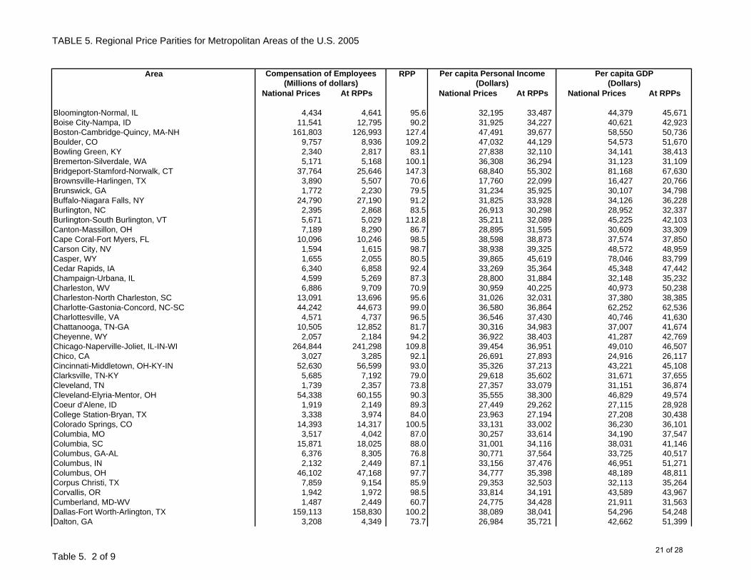
TABLE 5. Regional Price Parities for Metropolitan Areas of the U.S. 2005
Area RPP
National Prices At RPPs National Prices At RPPs National Prices At RPPs
Compensation of Employees(Millions of dollars)
Per capita Personal Income(Dollars) (Dollars)
Per capita GDP
Bloomington-Normal, IL 4,434 4,641 95.6 32,195 33,487 44,379 45,671 Boise City-Nampa, ID 11,541 12,795 90.2 31,925 34,227 40,621 42,923 Boston-Cambridge-Quincy, MA-NH 161,803 126,993 127.4 47,491 39,677 58,550 50,736 Boulder, CO 9,757 8,936 109.2 47,032 44,129 54,573 51,670 Bowling Green, KY 2,340 2,817 83.1 27,838 32,110 34,141 38,413 Bremerton-Silverdale, WA 5,171 5,168 100.1 36,308 36,294 31,123 31,109 Bridgeport-Stamford-Norwalk, CT 37,764 25,646 147.3 68,840 55,302 81,168 67,630 Brownsville-Harlingen, TX 3,890 5,507 70.6 17,760 22,099 16,427 20,766 Brunswick, GA 1,772 2,230 79.5 31,234 35,925 30,107 34,798 Buffalo-Niagara Falls, NY 24,790 27,190 91.2 31,825 33,928 34,126 36,228 Burlington, NC 2,395 2,868 83.5 26,913 30,298 28,952 32,337 Burlington-South Burlington, VT 5,671 5,029 112.8 35,211 32,089 45,225 42,103 Canton-Massillon, OH 7,189 8,290 86.7 28,895 31,595 30,609 33,309 Cape Coral-Fort Myers, FL 10,096 10,246 98.5 38,598 38,873 37,574 37,850 Carson City, NV 1,594 1,615 98.7 38,938 39,325 48,572 48,959 Casper, WY 1,655 2,055 80.5 39,865 45,619 78,046 83,799 Cedar Rapids, IA 6,340 6,858 92.4 33,269 35,364 45,348 47,442 Champaign-Urbana, IL 4,599 5,269 87.3 28,800 31,884 32,148 35,232 Charleston, WV 6,886 9,709 70.9 30,959 40,225 40,973 50,238 Charleston-North Charleston, SC 13,091 13,696 95.6 31,026 32,031 37,380 38,385 Charlotte-Gastonia-Concord, NC-SC 44,242 44,673 99.0 36,580 36,864 62,252 62,536 Charlottesville, VA 4,571 4,737 96.5 36,546 37,430 40,746 41,630 Chattanooga, TN-GA 10,505 12,852 81.7 30,316 34,983 37,007 41,674 Cheyenne, WY 2,057 2,184 94.2 36,922 38,403 41,287 42,769 Chicago-Naperville-Joliet, IL-IN-WI 264,844 241,298 109.8 39,454 36,951 49,010 46,507 Chico, CA 3,027 3,285 92.1 26,691 27,893 24,916 26,117 Cincinnati-Middletown, OH-KY-IN 52,630 56,599 93.0 35,326 37,213 43,221 45,108 Clarksville, TN-KY 5,685 7,192 79.0 29,618 35,602 31,671 37,655 Cleveland, TN 1,739 2,357 73.8 27,357 33,079 31,151 36,874 Cleveland-Elyria-Mentor, OH 54,338 60,155 90.3 35,555 38,300 46,829 49,574 Coeur d'Alene, ID 1,919 2,149 89.3 27,449 29,262 27,115 28,928 College Station-Bryan, TX 3,338 3,974 84.0 23,963 27,194 27,208 30,438 Colorado Springs, CO 14,393 14,317 100.5 33,131 33,002 36,230 36,101 Columbia, MO 3,517 4,042 87.0 30,257 33,614 34,190 37,547 Columbia, SC 15,871 18,025 88.0 31,001 34,116 38,031 41,146 Columbus, GA-AL 6,376 8,305 76.8 30,771 37,564 33,725 40,517 Columbus, IN 2,132 2,449 87.1 33,156 37,476 46,951 51,271 Columbus, OH 46,102 47,168 97.7 34,777 35,398 48,189 48,811 Corpus Christi, TX 7,859 9,154 85.9 29,353 32,503 32,113 35,264 Corvallis, OR 1,942 1,972 98.5 33,814 34,191 43,589 43,967 Cumberland, MD-WV 1,487 2,449 60.7 24,775 34,428 21,911 31,563 Dallas-Fort Worth-Arlington, TX 159,113 158,830 100.2 38,089 38,041 54,296 54,248 Dalton, GA 3,208 4,349 73.7 26,984 35,721 42,662 51,399
Table 5. 2 of 921 of 28

TABLE 5. Regional Price Parities for Metropolitan Areas of the U.S. 2005
Area RPP
National Prices At RPPs National Prices At RPPs National Prices At RPPs
Compensation of Employees(Millions of dollars)
Per capita Personal Income(Dollars) (Dollars)
Per capita GDP
Danville, IL 1,354 1,962 69.0 24,719 32,148 25,080 32,509 Danville, VA 1,577 2,247 70.2 25,492 31,775 26,346 32,628 Davenport-Moline-Rock Island, IA-IL 8,662 10,264 84.4 32,405 36,696 39,490 43,780 Dayton, OH 20,291 22,942 88.4 31,739 34,893 38,551 41,704 Decatur, AL 2,481 3,417 72.6 29,401 35,762 32,235 38,596 Decatur, IL 2,716 3,755 72.3 32,649 42,136 43,408 52,895 Deltona-Daytona Beach-Ormond Beach, FL 6,486 7,395 87.7 28,329 30,197 22,821 24,688 Denver-Aurora, CO 70,028 71,206 98.3 42,476 42,974 55,592 56,090 Des Moines-West Des Moines, IA 15,384 15,465 99.5 37,650 37,805 59,476 59,630 Detroit-Warren-Livonia, MI 121,881 122,378 99.6 37,204 37,314 44,068 44,178 Dothan, AL 2,417 3,443 70.2 28,701 36,256 31,219 38,775 Dover, DE 2,980 3,346 89.1 27,881 30,424 36,913 39,456 Dubuque, IA 2,176 2,618 83.1 30,462 35,320 41,953 46,811 Duluth, MN-WI 5,394 7,055 76.5 29,515 35,571 31,314 37,369 Durham, NC 15,642 15,551 100.6 34,775 34,577 56,613 56,415 Eau Claire, WI 3,056 3,590 85.1 28,519 31,972 33,947 37,401 El Centro, CA 2,232 2,397 93.1 22,074 23,146 22,351 23,423 Elizabethtown, KY 2,564 3,062 83.7 29,500 34,011 36,111 40,622 Elkhart-Goshen, IN 6,017 6,784 88.7 31,826 35,790 48,482 52,446 Elmira, NY 1,651 2,003 82.4 27,567 31,546 27,906 31,885 El Paso, TX 10,821 14,071 76.9 24,081 28,644 30,851 35,413 Erie, PA 5,465 6,699 81.6 27,520 31,941 29,590 34,011 Eugene-Springfield, OR 6,288 6,702 93.8 29,209 30,440 31,016 32,248 Evansville, IN-KY 8,128 10,078 80.7 32,612 38,222 42,174 47,784 Fairbanks, AK 2,546 2,434 104.6 32,001 30,817 42,339 41,155 Fargo, ND-MN 4,587 5,237 87.6 33,108 36,600 45,436 48,928 Farmington, NM 2,166 3,045 71.1 24,675 31,878 51,939 59,142 Fayetteville, NC 9,242 10,540 87.7 31,110 34,869 36,931 40,691 Fayetteville-Springdale-Rogers, AR-MO 8,740 10,108 86.5 28,694 32,042 37,640 40,988 Flagstaff, AZ 2,303 2,684 85.8 28,008 31,068 29,930 32,989 Flint, MI 7,690 9,080 84.7 27,602 30,765 27,037 30,200 Florence, SC 3,740 4,917 76.1 27,641 33,622 32,137 38,118 Florence-Muscle Shoals, AL 2,060 2,804 73.5 25,741 30,983 24,159 29,401 Fond du Lac, WI 1,989 2,233 89.1 31,745 34,224 34,831 37,310 Fort Collins-Loveland, CO 5,999 5,789 103.6 33,886 33,128 35,187 34,429 Fort Smith, AR-OK 4,659 6,397 72.8 26,376 32,522 32,837 38,983 Fort Walton Beach-Crestview-Destin, FL 5,007 5,731 87.4 35,023 38,970 49,121 53,067 Fort Wayne, IN 9,378 10,989 85.3 30,813 34,809 38,474 42,470 Fresno, CA 14,820 14,852 99.8 26,052 26,088 28,693 28,729 Gadsden, AL 1,412 2,144 65.9 26,071 33,210 23,248 30,387 Gainesville, FL 5,569 6,295 88.5 29,663 32,592 33,175 36,104 Gainesville, GA 2,999 3,252 92.2 27,458 28,990 34,148 35,680 Glens Falls, NY 2,215 2,434 91.0 28,282 29,993 26,325 28,036
Table 5. 3 of 922 of 28
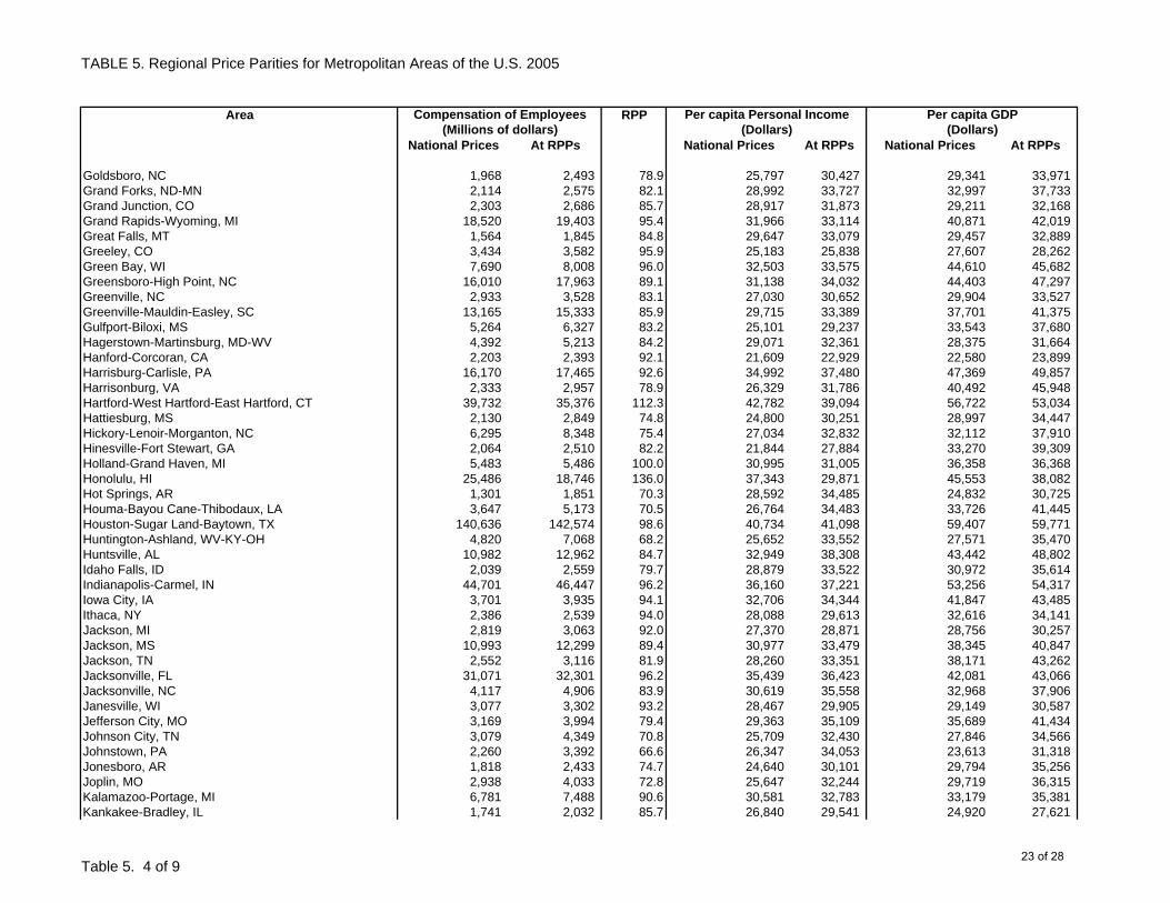
TABLE 5. Regional Price Parities for Metropolitan Areas of the U.S. 2005
Area RPP
National Prices At RPPs National Prices At RPPs National Prices At RPPs
Compensation of Employees(Millions of dollars)
Per capita Personal Income(Dollars) (Dollars)
Per capita GDP
Goldsboro, NC 1,968 2,493 78.9 25,797 30,427 29,341 33,971 Grand Forks, ND-MN 2,114 2,575 82.1 28,992 33,727 32,997 37,733 Grand Junction, CO 2,303 2,686 85.7 28,917 31,873 29,211 32,168 Grand Rapids-Wyoming, MI 18,520 19,403 95.4 31,966 33,114 40,871 42,019 Great Falls, MT 1,564 1,845 84.8 29,647 33,079 29,457 32,889 Greeley, CO 3,434 3,582 95.9 25,183 25,838 27,607 28,262 Green Bay, WI 7,690 8,008 96.0 32,503 33,575 44,610 45,682 Greensboro-High Point, NC 16,010 17,963 89.1 31,138 34,032 44,403 47,297 Greenville, NC 2,933 3,528 83.1 27,030 30,652 29,904 33,527 Greenville-Mauldin-Easley, SC 13,165 15,333 85.9 29,715 33,389 37,701 41,375 Gulfport-Biloxi, MS 5,264 6,327 83.2 25,101 29,237 33,543 37,680 Hagerstown-Martinsburg, MD-WV 4,392 5,213 84.2 29,071 32,361 28,375 31,664 Hanford-Corcoran, CA 2,203 2,393 92.1 21,609 22,929 22,580 23,899 Harrisburg-Carlisle, PA 16,170 17,465 92.6 34,992 37,480 47,369 49,857 Harrisonburg, VA 2,333 2,957 78.9 26,329 31,786 40,492 45,948 Hartford-West Hartford-East Hartford, CT 39,732 35,376 112.3 42,782 39,094 56,722 53,034 Hattiesburg, MS 2,130 2,849 74.8 24,800 30,251 28,997 34,447 Hickory-Lenoir-Morganton, NC 6,295 8,348 75.4 27,034 32,832 32,112 37,910 Hinesville-Fort Stewart, GA 2,064 2,510 82.2 21,844 27,884 33,270 39,309 Holland-Grand Haven, MI 5,483 5,486 100.0 30,995 31,005 36,358 36,368 Honolulu, HI 25,486 18,746 136.0 37,343 29,871 45,553 38,082 Hot Springs, AR 1,301 1,851 70.3 28,592 34,485 24,832 30,725 Houma-Bayou Cane-Thibodaux, LA 3,647 5,173 70.5 26,764 34,483 33,726 41,445 Houston-Sugar Land-Baytown, TX 140,636 142,574 98.6 40,734 41,098 59,407 59,771 Huntington-Ashland, WV-KY-OH 4,820 7,068 68.2 25,652 33,552 27,571 35,470 Huntsville, AL 10,982 12,962 84.7 32,949 38,308 43,442 48,802 Idaho Falls, ID 2,039 2,559 79.7 28,879 33,522 30,972 35,614 Indianapolis-Carmel, IN 44,701 46,447 96.2 36,160 37,221 53,256 54,317 Iowa City, IA 3,701 3,935 94.1 32,706 34,344 41,847 43,485 Ithaca, NY 2,386 2,539 94.0 28,088 29,613 32,616 34,141 Jackson, MI 2,819 3,063 92.0 27,370 28,871 28,756 30,257 Jackson, MS 10,993 12,299 89.4 30,977 33,479 38,345 40,847 Jackson, TN 2,552 3,116 81.9 28,260 33,351 38,171 43,262 Jacksonville, FL 31,071 32,301 96.2 35,439 36,423 42,081 43,066 Jacksonville, NC 4,117 4,906 83.9 30,619 35,558 32,968 37,906 Janesville, WI 3,077 3,302 93.2 28,467 29,905 29,149 30,587 Jefferson City, MO 3,169 3,994 79.4 29,363 35,109 35,689 41,434 Johnson City, TN 3,079 4,349 70.8 25,709 32,430 27,846 34,566 Johnstown, PA 2,260 3,392 66.6 26,347 34,053 23,613 31,318 Jonesboro, AR 1,818 2,433 74.7 24,640 30,101 29,794 35,256 Joplin, MO 2,938 4,033 72.8 25,647 32,244 29,719 36,315 Kalamazoo-Portage, MI 6,781 7,488 90.6 30,581 32,783 33,179 35,381 Kankakee-Bradley, IL 1,741 2,032 85.7 26,840 29,541 24,920 27,621
Table 5. 4 of 923 of 28
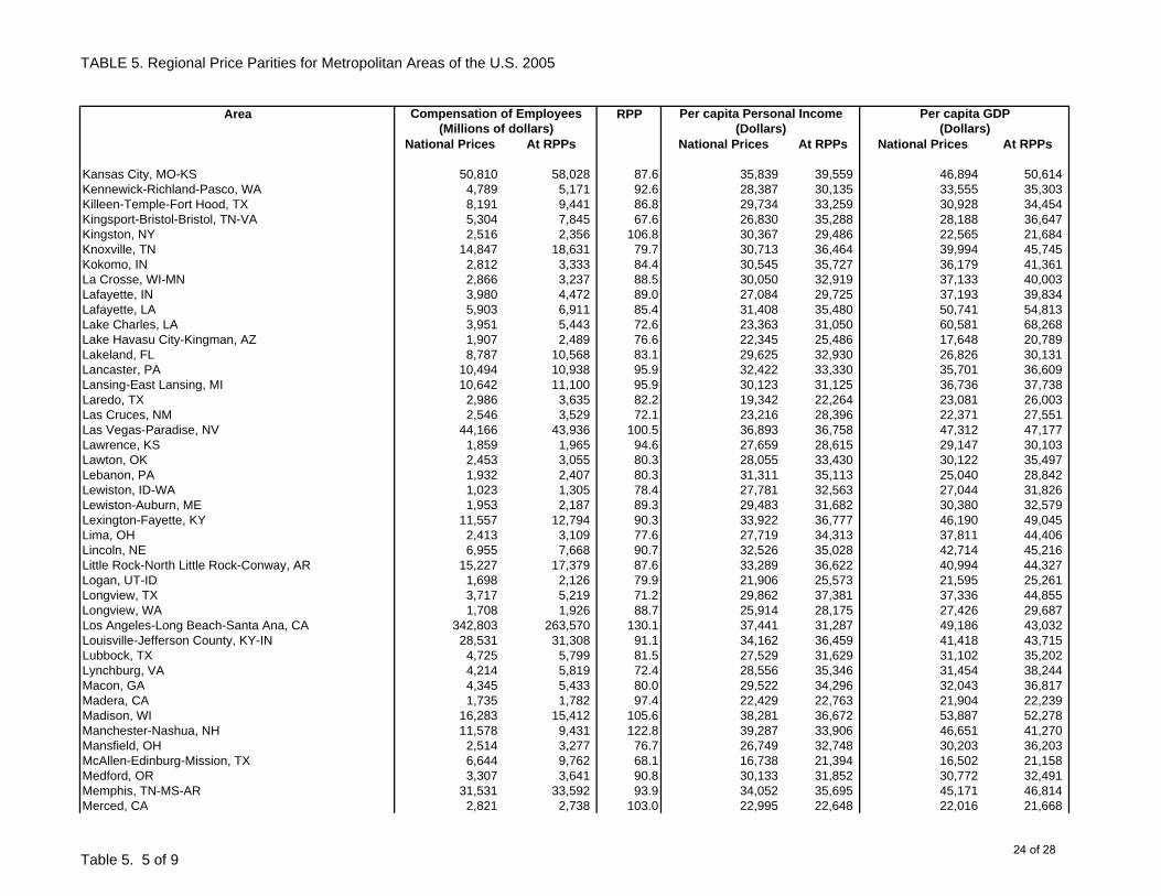
TABLE 5. Regional Price Parities for Metropolitan Areas of the U.S. 2005
Area RPP
National Prices At RPPs National Prices At RPPs National Prices At RPPs
Compensation of Employees(Millions of dollars)
Per capita Personal Income(Dollars) (Dollars)
Per capita GDP
Kansas City, MO-KS 50,810 58,028 87.6 35,839 39,559 46,894 50,614 Kennewick-Richland-Pasco, WA 4,789 5,171 92.6 28,387 30,135 33,555 35,303 Killeen-Temple-Fort Hood, TX 8,191 9,441 86.8 29,734 33,259 30,928 34,454 Kingsport-Bristol-Bristol, TN-VA 5,304 7,845 67.6 26,830 35,288 28,188 36,647 Kingston, NY 2,516 2,356 106.8 30,367 29,486 22,565 21,684 Knoxville, TN 14,847 18,631 79.7 30,713 36,464 39,994 45,745 Kokomo, IN 2,812 3,333 84.4 30,545 35,727 36,179 41,361 La Crosse, WI-MN 2,866 3,237 88.5 30,050 32,919 37,133 40,003 Lafayette, IN 3,980 4,472 89.0 27,084 29,725 37,193 39,834 Lafayette, LA 5,903 6,911 85.4 31,408 35,480 50,741 54,813 Lake Charles, LA 3,951 5,443 72.6 23,363 31,050 60,581 68,268 Lake Havasu City-Kingman, AZ 1,907 2,489 76.6 22,345 25,486 17,648 20,789 Lakeland, FL 8,787 10,568 83.1 29,625 32,930 26,826 30,131 Lancaster, PA 10,494 10,938 95.9 32,422 33,330 35,701 36,609 Lansing-East Lansing, MI 10,642 11,100 95.9 30,123 31,125 36,736 37,738 Laredo, TX 2,986 3,635 82.2 19,342 22,264 23,081 26,003 Las Cruces, NM 2,546 3,529 72.1 23,216 28,396 22,371 27,551 Las Vegas-Paradise, NV 44,166 43,936 100.5 36,893 36,758 47,312 47,177 Lawrence, KS 1,859 1,965 94.6 27,659 28,615 29,147 30,103 Lawton, OK 2,453 3,055 80.3 28,055 33,430 30,122 35,497 Lebanon, PA 1,932 2,407 80.3 31,311 35,113 25,040 28,842 Lewiston, ID-WA 1,023 1,305 78.4 27,781 32,563 27,044 31,826 Lewiston-Auburn, ME 1,953 2,187 89.3 29,483 31,682 30,380 32,579 Lexington-Fayette, KY 11,557 12,794 90.3 33,922 36,777 46,190 49,045 Lima, OH 2,413 3,109 77.6 27,719 34,313 37,811 44,406 Lincoln, NE 6,955 7,668 90.7 32,526 35,028 42,714 45,216 Little Rock-North Little Rock-Conway, AR 15,227 17,379 87.6 33,289 36,622 40,994 44,327 Logan, UT-ID 1,698 2,126 79.9 21,906 25,573 21,595 25,261 Longview, TX 3,717 5,219 71.2 29,862 37,381 37,336 44,855 Longview, WA 1,708 1,926 88.7 25,914 28,175 27,426 29,687 Los Angeles-Long Beach-Santa Ana, CA 342,803 263,570 130.1 37,441 31,287 49,186 43,032 Louisville-Jefferson County, KY-IN 28,531 31,308 91.1 34,162 36,459 41,418 43,715 Lubbock, TX 4,725 5,799 81.5 27,529 31,629 31,102 35,202 Lynchburg, VA 4,214 5,819 72.4 28,556 35,346 31,454 38,244 Macon, GA 4,345 5,433 80.0 29,522 34,296 32,043 36,817 Madera, CA 1,735 1,782 97.4 22,429 22,763 21,904 22,239 Madison, WI 16,283 15,412 105.6 38,281 36,672 53,887 52,278 Manchester-Nashua, NH 11,578 9,431 122.8 39,287 33,906 46,651 41,270 Mansfield, OH 2,514 3,277 76.7 26,749 32,748 30,203 36,203 McAllen-Edinburg-Mission, TX 6,644 9,762 68.1 16,738 21,394 16,502 21,158 Medford, OR 3,307 3,641 90.8 30,133 31,852 30,772 32,491 Memphis, TN-MS-AR 31,531 33,592 93.9 34,052 35,695 45,171 46,814 Merced, CA 2,821 2,738 103.0 22,995 22,648 22,016 21,668
Table 5. 5 of 924 of 28

TABLE 5. Regional Price Parities for Metropolitan Areas of the U.S. 2005
Area RPP
National Prices At RPPs National Prices At RPPs National Prices At RPPs
Compensation of Employees(Millions of dollars)
Per capita Personal Income(Dollars) (Dollars)
Per capita GDP
Miami-Fort Lauderdale-Pompano Beach, FL 122,333 112,244 109.0 38,342 36,469 43,006 41,133 Michigan City-La Porte, IN 1,877 2,218 84.6 27,005 30,132 28,722 31,848 Midland, TX 2,895 3,478 83.2 42,615 47,451 63,813 68,649 Milwaukee-Waukesha-West Allis, WI 42,900 46,859 91.6 37,361 39,940 47,743 50,322 Minneapolis-St. Paul-Bloomington, MN-WI 101,909 96,224 105.9 42,457 40,645 54,565 52,753 Missoula, MT 2,165 2,402 90.1 30,101 32,420 38,732 41,052 Mobile, AL 7,673 9,371 81.9 25,211 29,475 32,093 36,356 Modesto, CA 8,003 7,392 108.3 26,995 25,775 27,700 26,480 Monroe, LA 2,915 3,759 77.6 27,405 32,337 32,960 37,892 Monroe, MI 2,291 2,380 96.3 31,029 31,615 24,792 25,378 Montgomery, AL 7,967 9,790 81.4 31,356 36,472 36,772 41,889 Morgantown, WV 2,398 3,393 70.7 28,203 36,768 36,845 45,411 Morristown, TN 2,045 2,507 81.6 24,312 27,869 26,275 29,832 Mount Vernon-Anacortes, WA 2,057 2,058 100.0 31,962 31,968 40,981 40,988 Muncie, IN 2,032 2,599 78.2 26,535 31,393 27,485 32,343 Muskegon-Norton Shores, MI 2,839 3,250 87.4 25,626 27,986 25,996 28,356 Myrtle Beach-Conway-North Myrtle Beach, SC 4,013 4,890 82.1 26,745 30,584 37,244 41,083 Napa, CA 3,619 2,646 136.8 45,223 37,765 49,184 41,725 Naples-Marco Island, FL 6,524 6,021 108.4 54,166 52,526 44,706 43,066 Nashville-Davidson-Murfreesboro-Franklin, TN 36,480 38,916 93.7 36,056 37,736 47,298 48,977 New Haven-Milford, CT 20,979 17,122 122.5 39,354 34,772 40,717 36,135 New Orleans-Metairie-Kenner, LA 26,915 30,293 88.8 19,926 22,505 47,254 49,833 New York-Northern New Jersey-Long Island, NY-NJ-PA 597,444 417,241 143.2 46,221 36,614 57,117 47,510 Niles-Benton Harbor, MI 2,975 3,613 82.3 29,361 33,344 30,518 34,501 Norwich-New London, CT 7,803 6,972 111.9 39,181 36,049 43,441 40,309 Ocala, FL 3,940 5,051 78.0 27,720 31,402 22,137 25,819 Ocean City, NJ 1,778 1,661 107.0 39,059 37,874 40,764 39,579 Odessa, TX 2,296 3,287 69.9 26,115 34,074 33,305 41,264 Ogden-Clearfield, UT 8,434 9,435 89.4 28,148 30,183 27,899 29,934 Oklahoma City, OK 24,806 28,565 86.8 33,243 36,494 40,316 43,567 Olympia, WA 4,533 4,636 97.8 34,204 34,656 31,164 31,615 Omaha-Council Bluffs, NE-IA 21,472 22,051 97.4 37,869 38,582 48,739 49,452 Orlando-Kissimmee, FL 47,381 47,181 100.4 31,828 31,725 46,051 45,948 Oshkosh-Neenah, WI 4,478 4,860 92.1 32,572 34,962 42,152 44,541 Owensboro, KY 2,009 2,621 76.6 28,046 33,569 33,269 38,791 Oxnard-Thousand Oaks-Ventura, CA 19,139 14,783 129.5 40,845 35,337 40,636 35,128 Palm Bay-Melbourne-Titusville, FL 10,694 11,692 91.5 32,314 34,208 30,286 32,180 Palm Coast, FL 699 769 90.9 28,474 29,400 30,025 30,950 Panama City-Lynn Haven, FL 3,384 4,082 82.9 30,378 34,698 34,880 39,200 Parkersburg-Marietta-Vienna, WV-OH 2,964 4,059 73.0 26,643 33,411 30,368 37,136 Pascagoula, MS 2,710 3,298 82.2 25,248 29,035 25,036 28,824 Pensacola-Ferry Pass-Brent, FL 7,818 9,234 84.7 28,267 31,447 26,886 30,066 Peoria, IL 9,214 10,782 85.5 33,540 37,808 39,243 43,511
Table 5. 6 of 925 of 28

TABLE 5. Regional Price Parities for Metropolitan Areas of the U.S. 2005
Area RPP
National Prices At RPPs National Prices At RPPs National Prices At RPPs
Compensation of Employees(Millions of dollars)
Per capita Personal Income(Dollars) (Dollars)
Per capita GDP
Philadelphia-Camden-Wilmington, PA-NJ-DE-MD 162,937 148,402 109.8 40,948 38,438 50,900 48,391 Phoenix-Mesa-Scottsdale, AZ 89,825 86,846 103.4 32,660 31,893 41,388 40,620 Pine Bluff, AR 1,687 2,253 74.9 23,456 28,912 26,292 31,748 Pittsburgh, PA 55,648 63,666 87.4 36,159 39,535 42,945 46,321 Pittsfield, MA 2,873 3,171 90.6 36,614 38,891 40,872 43,149 Pocatello, ID 1,440 1,834 78.5 24,358 28,937 27,504 32,082 Portland-South Portland-Biddeford, ME 12,393 11,590 106.9 35,425 33,855 43,332 41,762 Portland-Vancouver-Beaverton, OR-WA 52,423 51,218 102.4 34,921 34,345 45,617 45,041 Port St. Lucie, FL 5,602 6,023 93.0 36,086 37,206 27,144 28,263 Poughkeepsie-Newburgh-Middletown, NY 12,694 9,608 132.1 34,164 29,509 28,847 24,192 Prescott, AZ 2,224 2,683 82.9 25,460 27,781 19,875 22,196 Providence-New Bedford-Fall River, RI-MA 34,689 30,925 112.2 35,412 33,075 36,855 34,517 Provo-Orem, UT 6,525 7,640 85.4 21,127 23,531 24,217 26,621 Pueblo, CO 2,175 2,660 81.8 25,438 28,672 22,610 25,845 Punta Gorda, FL 1,711 2,011 85.1 30,886 32,844 21,301 23,259 Racine, WI 3,854 4,283 90.0 33,404 35,621 33,043 35,260 Raleigh-Cary, NC 23,589 22,135 106.6 35,585 34,064 45,385 43,863 Rapid City, SD 2,476 2,927 84.6 32,287 36,104 35,643 39,460 Reading, PA 7,874 8,331 94.5 31,617 32,778 32,859 34,020 Redding, CA 2,840 2,877 98.7 29,010 29,219 28,518 28,728 Reno-Sparks, NV 10,598 10,163 104.3 42,219 41,118 46,465 45,364 Richmond, VA 32,386 33,396 97.0 37,082 37,942 47,286 48,145 Riverside-San Bernardino-Ontario, CA 59,846 55,279 108.3 26,818 25,642 26,160 24,984 Roanoke, VA 6,937 8,824 78.6 32,308 38,768 39,061 45,522 Rochester, MN 5,308 5,570 95.3 36,886 38,373 45,315 46,802 Rochester, NY 24,753 25,069 98.7 34,294 34,600 40,545 40,851 Rockford, IL 7,055 7,410 95.2 28,311 29,355 32,028 33,071 Rocky Mount, NC 2,593 3,341 77.6 27,004 32,201 38,346 43,543 Rome, GA 1,867 2,637 70.8 28,705 36,879 32,683 40,857 Sacramento-Arden-Arcade-Roseville, CA 51,426 42,498 121.0 35,318 30,937 41,599 37,219 Saginaw-Saginaw Township North, MI 4,357 5,289 82.4 27,246 31,757 31,258 35,769 St. Cloud, MN 3,944 4,393 89.8 28,741 31,214 37,540 40,013 St. George, UT 1,620 2,070 78.3 23,353 27,129 24,110 27,885 St. Joseph, MO-KS 2,116 2,902 72.9 26,345 32,806 28,864 35,325 St. Louis, MO-IL 69,876 79,210 88.2 35,991 39,354 41,853 45,216 Salem, OR 6,487 7,088 91.5 27,699 29,311 29,884 31,495 Salinas, CA 8,749 6,815 128.4 36,137 31,405 40,175 35,444 Salisbury, MD 2,227 2,665 83.6 28,016 31,791 29,827 33,601 Salt Lake City, UT 27,847 29,628 94.0 33,469 35,167 48,244 49,942 San Angelo, TX 1,914 2,486 77.0 28,519 33,872 29,491 34,843 San Antonio, TX 37,877 42,218 89.7 31,189 33,494 35,567 37,872 San Diego-Carlsbad-San Marcos, CA 82,957 67,702 122.5 40,383 35,197 49,719 44,533 Sandusky, OH 1,680 2,001 83.9 33,171 37,298 37,385 41,511
Table 5. 7 of 926 of 28
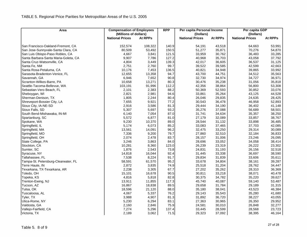
TABLE 5. Regional Price Parities for Metropolitan Areas of the U.S. 2005
Area RPP
National Prices At RPPs National Prices At RPPs National Prices At RPPs
Compensation of Employees(Millions of dollars)
Per capita Personal Income(Dollars) (Dollars)
Per capita GDP
San Francisco-Oakland-Fremont, CA 152,574 108,322 140.9 54,191 43,518 64,663 53,991 San Jose-Sunnyvale-Santa Clara, CA 80,509 53,492 150.5 51,277 35,871 70,276 54,870 San Luis Obispo-Paso Robles, CA 4,667 3,841 121.5 33,959 30,762 36,483 33,285 Santa Barbara-Santa Maria-Goleta, CA 9,907 7,786 127.2 40,968 35,703 43,058 37,792 Santa Cruz-Watsonville, CA 4,804 3,449 139.3 42,017 36,605 36,537 31,125 Santa Fe, NM 2,751 2,760 99.7 39,522 39,585 42,599 42,663 Santa Rosa-Petaluma, CA 10,176 7,453 136.5 40,821 34,948 39,865 33,992 Sarasota-Bradenton-Venice, FL 12,655 13,358 94.7 43,700 44,751 34,512 35,563 Savannah, GA 6,946 7,652 90.8 32,730 34,974 34,727 36,971 Scranton-Wilkes-Barre, PA 10,658 13,271 80.3 30,476 35,238 31,056 35,818 Seattle-Tacoma-Bellevue, WA 103,191 91,996 112.2 42,356 38,864 56,800 53,308 Sebastian-Vero Beach, FL 2,101 2,383 88.2 50,369 52,593 30,852 33,076 Sheboygan, WI 2,821 2,981 94.6 33,861 35,264 43,125 44,528 Sherman-Denison, TX 1,805 2,244 80.4 26,046 29,835 24,635 28,425 Shreveport-Bossier City, LA 7,655 9,921 77.2 30,543 36,478 46,958 52,893 Sioux City, IA-NE-SD 2,916 3,586 81.3 29,444 34,190 36,402 41,148 Sioux Falls, SD 5,307 5,697 93.2 35,276 37,088 56,689 58,501 South Bend-Mishawaka, IN-MI 6,140 7,054 87.0 31,741 34,634 35,357 38,250 Spartanburg, SC 5,572 6,877 81.0 27,179 32,089 33,857 38,767 Spokane, WA 9,230 10,370 89.0 28,544 31,132 33,898 36,485 Springfield, IL 5,174 6,073 85.2 33,083 37,465 37,703 42,085 Springfield, MA 13,561 14,091 96.2 32,475 33,250 29,314 30,089 Springfield, MO 7,336 9,200 79.7 27,860 32,510 32,184 36,833 Springfield, OH 2,074 2,478 83.7 28,157 31,006 23,246 26,095 State College, PA 3,246 3,863 84.0 28,696 33,052 34,058 38,414 Stockton, CA 10,281 8,360 123.0 26,239 23,319 26,222 23,302 Sumter, SC 1,876 2,543 73.8 24,831 31,193 26,156 32,518 Syracuse, NY 14,818 16,044 92.4 31,445 33,338 36,697 38,590 Tallahassee, FL 7,538 8,224 91.7 29,834 31,839 33,606 35,611 Tampa-St. Petersburg-Clearwater, FL 58,591 61,570 95.2 33,678 34,804 38,161 39,287 Terre Haute, IN 2,872 3,835 74.9 25,518 31,204 28,762 34,447 Texarkana, TX-Texarkana, AR 2,238 3,305 67.7 27,202 35,262 28,310 36,369 Toledo, OH 15,101 16,678 90.5 30,811 33,218 38,071 40,478 Topeka, KS 4,816 5,818 82.8 30,375 34,782 35,220 39,627 Trenton-Ewing, NJ 13,911 11,855 117.3 45,740 40,087 59,140 53,487 Tucson, AZ 16,867 18,838 89.5 29,658 31,784 29,189 31,315 Tulsa, OK 18,596 21,120 88.0 35,180 38,041 43,523 46,384 Tuscaloosa, AL 4,067 5,337 76.2 29,143 35,543 35,280 41,680 Tyler, TX 3,988 4,907 81.3 31,892 36,720 38,227 43,055 Utica-Rome, NY 5,230 6,294 83.1 27,363 30,965 26,350 29,952 Valdosta, GA 2,160 2,846 75.9 24,581 30,010 26,848 32,277 Vallejo-Fairfield, CA 7,274 5,296 137.4 33,445 28,599 28,568 23,723 Victoria, TX 2,189 3,062 71.5 29,323 37,092 38,395 46,164
Table 5. 8 of 927 of 28

TABLE 5. Regional Price Parities for Metropolitan Areas of the U.S. 2005
Area RPP
National Prices At RPPs National Prices At RPPs National Prices At RPPs
Compensation of Employees(Millions of dollars)
Per capita Personal Income(Dollars) (Dollars)
Per capita GDP
Vineland-Millville-Bridgeton, NJ 2,937 2,930 100.2 27,378 27,331 29,603 29,557 Virginia Beach-Norfolk-Newport News, VA-NC 42,244 42,967 98.3 33,259 33,698 40,426 40,864 Visalia-Porterville, CA 5,445 6,015 90.5 23,654 25,055 23,786 25,188 Waco, TX 4,263 5,296 80.5 27,091 31,694 30,560 35,163 Warner Robins, GA 3,143 3,752 83.8 28,507 33,342 34,794 39,629 Washington-Arlington-Alexandria, DC-VA-MD-WV 214,825 184,220 116.6 49,442 43,582 66,510 60,650 Waterloo-Cedar Falls, IA 3,644 4,531 80.4 30,514 35,971 41,142 46,599 Wausau, WI 3,087 3,558 86.8 32,148 35,831 40,289 43,972 Weirton-Steubenville, WV-OH 1,946 3,119 62.4 25,982 35,337 26,599 35,955 Wenatchee, WA 1,841 2,176 84.6 27,671 30,915 31,325 34,569 Wheeling, WV-OH 2,611 4,167 62.7 27,764 38,310 29,913 40,460 Wichita, KS 13,726 15,739 87.2 34,491 37,933 37,942 41,384 Wichita Falls, TX 2,705 3,514 77.0 29,760 35,156 32,971 38,368 Williamsport, PA 2,106 2,619 80.4 27,285 31,642 28,793 33,150 Wilmington, NC 5,526 6,242 88.5 29,620 31,878 36,916 39,174 Winchester, VA-WV 2,399 2,686 89.3 29,847 32,322 38,017 40,492 Winston-Salem, NC 10,060 11,427 88.0 32,680 35,741 46,851 49,912 Worcester, MA 16,865 14,970 112.7 36,666 34,229 32,857 30,420 Yakima, WA 3,649 4,500 81.1 25,141 28,860 27,016 30,735 York-Hanover, PA 8,526 9,044 94.3 32,377 33,650 33,095 34,369 Youngstown-Warren-Boardman, OH-PA 10,089 12,951 77.9 27,927 32,850 28,689 33,612 Yuba City, CA 2,169 2,228 97.4 25,827 26,206 24,482 24,861 Yuma, AZ 2,573 3,772 68.2 21,081 27,721 22,744 29,384
Max 597,444 417,241 150.5 68,840 55,302 81,168 83,799 Min 699 769 60.7 16,738 21,394 16,427 20,766 Range 596,745 416,472 89.8 52,102 33,908 64,741 63,034
Table 5. 9 of 928 of 28