essays on economic growth and the economics of innovation
TRANSCRIPT
University of Pennsylvania University of Pennsylvania
ScholarlyCommons ScholarlyCommons
Publicly Accessible Penn Dissertations
2018
Essays On Economic Growth And The Economics Of Innovation Essays On Economic Growth And The Economics Of Innovation
Pengfei Han University of Pennsylvania, [email protected]
Follow this and additional works at: https://repository.upenn.edu/edissertations
Part of the Economics Commons
Recommended Citation Recommended Citation Han, Pengfei, "Essays On Economic Growth And The Economics Of Innovation" (2018). Publicly Accessible Penn Dissertations. 2941. https://repository.upenn.edu/edissertations/2941
This paper is posted at ScholarlyCommons. https://repository.upenn.edu/edissertations/2941 For more information, please contact [email protected].

Essays On Economic Growth And The Economics Of Innovation Essays On Economic Growth And The Economics Of Innovation
Abstract Abstract In my dissertation, I study how legal institutions and financial system affect innovation and their impact on economic growth. This dissertation consists of two chapters. The themes of chapter 1 and 2 are intellectual property rights and the venture capital system, respectively.
Chapter 1 studies the impact of intellectual property rights on the business scope of firms. Stronger intellectual property rights induce specialization and contribute to economic growth. In the United States, a sweeping legal reform in 1982 created a more pro-patent legal environment. This legal reform fostered specialization and enhanced firm performance. Around the world, countries experience faster economic growth when their innovating sectors are characterized by a higher level of specialization. An endogenous growth model with endogenous firm boundaries is developed to disentangle the relationship between legal institutions, firm boundary decisions, and economic growth. I characterize the optimal strength of patent rights and evaluate the actual patent law enforcement in the United States. The pro-patent legal reform in 1982 was welfare-enhancing, but it was too extreme. Swinging back the legal pendulum and weakening patent rights can improve welfare.
Chapter 2 evaluates the contribution of venture capital (VC) to promoting entrepreneurship and spawning innovation. We assemble the stylized facts of venture capital, innovation, and economic growth. Funding by venture capitalists is positively associated with patenting activity. VC-backed firms have higher IPO values when they are floated. Following flotation, they have higher R&D-to-sales ratios and grow faster in terms of employment and sales. At the country level, VC investment is positively linked with economic growth. The relationship between venture capital and growth is examined using an endogenous growth model incorporating dynamic contracts between entrepreneurs and venture capitalists. The model is matched with stylized facts about venture capital; viz., statistics by funding round concerning the success rate, failure rate, investment rate, equity shares, and the value of an IPO. We examine how the innovative activity is affected by the capital gains tax rate. Raising capital gains taxation reduces growth and welfare.
Degree Type Degree Type Dissertation
Degree Name Degree Name Doctor of Philosophy (PhD)
Graduate Group Graduate Group Economics
First Advisor First Advisor Jeremy Greenwood
Keywords Keywords Economic Growth, Firm Boundaries, Innovation, Intellectual Property Rights, Startups, Venture Capital
Subject Categories Subject Categories Economics
This dissertation is available at ScholarlyCommons: https://repository.upenn.edu/edissertations/2941

ESSAYS ON ECONOMIC GROWTH AND THE ECONOMICS OF INNOVATION
Pengfei Han
A DISSERTATION
in
Economics
Presented to the Faculties of the University of Pennsylvania
in
Partial Fulfillment of the Requirements for the
Degree of Doctor of Philosophy
2018
Supervisor of Dissertation
Jeremy Greenwood, Professor of Economics
Graduate Group Chairperson
Jesus Fernandez-Villaverde, Professor of Economics
Dissertation Committee
Joao F. Gomes, Howard Butcher III Professor of Finance
Harold L. Cole, Professor of Economics

ESSAYS ON ECONOMIC GROWTH AND THE ECONOMICS OF INNOVATION
c© COPYRIGHT
2018
Pengfei Han
This work is licensed under the
Creative Commons Attribution
NonCommercial-ShareAlike 3.0
License
To view a copy of this license, visit
http://creativecommons.org/licenses/by-nc-sa/3.0/

ACKNOWLEDGEMENT
I owe my deepest gratitude to my advisor Jeremy Greenwood, a role model for both research
and work ethic. You are always spurring me to work hard, Jeremy, and you are always lifting
my spirits when I am down. I am tremendously grateful for your invaluable guidance,
continuous support, and funny jokes. I am deeply indebted to my mentor Joao Gomes. You
are a thoughtful gentleman, Joao, and I have learned enormously from your broad horizon
and deep insights. I am highly grateful to my committee member Harold Cole. Thank you
for all your patient mentoring and helpful advice, Hal.
I am also grateful to Harun Alp, Murat Celik, Iourii Manovskii, Enrique Mendoza, Ezra
Oberfield, Guillermo Ordonez, Gokhan Oz, and Juan Sanchez, for the valuable discussion
and feedback during my Ph.D. study.
I owe special gratitude to my beloved family, particularly my mother Fengxia Li and my
wife Ying Zhang. Thank you for staying together with me through all the ups and downs.
Without you, I would not have become the person I am now. You are the most precious
treasure in my life.
I am very lucky to meet so many caring and cheerful friends, particularly Victor Ayala,
Minsu Chang, Luis Guirola, Mallick Hossain, Daniel Kim, Joonbae Lee, Maria Jose Or-
raca, Eugenio Rojas, Takeaki Sunada, and Junyuan Zou. Our days in Philadelphia will be
cherished memories in the rest of my life.
Many thanks to you all.
iii

ABSTRACT
ESSAYS ON ECONOMIC GROWTH AND THE ECONOMICS OF INNOVATION
Pengfei Han
Jeremy Greenwood
In my dissertation, I study how legal institutions and financial system affect innovation and
their impact on economic growth. This dissertation consists of two chapters. The themes of
chapter 1 and 2 are intellectual property rights and the venture capital system, respectively.
Chapter 1 studies the impact of intellectual property rights on the business scope of firms.
Stronger intellectual property rights induce specialization and contribute to economic growth.
In the United States, a sweeping legal reform in 1982 created a more pro-patent legal envi-
ronment. This legal reform fostered specialization and enhanced firm performance. Around
the world, countries experience faster economic growth when their innovating sectors are
characterized by a higher level of specialization. An endogenous growth model with endoge-
nous firm boundaries is developed to disentangle the relationship between legal institutions,
firm boundary decisions, and economic growth. I characterize the optimal strength of patent
rights and evaluate the actual patent law enforcement in the United States. The pro-patent
legal reform in 1982 was welfare-enhancing, but it was too extreme. Swinging back the legal
pendulum and weakening patent rights can improve welfare.
Chapter 2 evaluates the contribution of venture capital (VC) to promoting entrepreneur-
ship and spawning innovation. We assemble the stylized facts of venture capital, innovation,
and economic growth. Funding by venture capitalists is positively associated with patenting
activity. VC-backed firms have higher IPO values when they are floated. Following flota-
tion, they have higher R&D-to-sales ratios and grow faster in terms of employment and
sales. At the country level, VC investment is positively linked with economic growth. The
relationship between venture capital and growth is examined using an endogenous growth
iv

model incorporating dynamic contracts between entrepreneurs and venture capitalists. The
model is matched with stylized facts about venture capital; viz., statistics by funding round
concerning the success rate, failure rate, investment rate, equity shares, and the value of
an IPO. We examine how the innovative activity is affected by the capital gains tax rate.
Raising capital gains taxation reduces growth and welfare.
v

TABLE OF CONTENTS
ACKNOWLEDGEMENT . . . . . . . . . . . . . . . . . . . . . . . . . . . . . . . . . iii
ABSTRACT . . . . . . . . . . . . . . . . . . . . . . . . . . . . . . . . . . . . . . . . iv
LIST OF TABLES . . . . . . . . . . . . . . . . . . . . . . . . . . . . . . . . . . . . . viii
LIST OF ILLUSTRATIONS . . . . . . . . . . . . . . . . . . . . . . . . . . . . . . . x
CHAPTER 1 : Intellectual Property Rights and the Theory of the Innovating Firm 1
1.1 Introduction . . . . . . . . . . . . . . . . . . . . . . . . . . . . . . . . . . . . 1
1.2 Background . . . . . . . . . . . . . . . . . . . . . . . . . . . . . . . . . . . . 7
1.3 Model . . . . . . . . . . . . . . . . . . . . . . . . . . . . . . . . . . . . . . . 14
1.4 Quantitative Analysis . . . . . . . . . . . . . . . . . . . . . . . . . . . . . . 28
1.5 Empirical Evidence . . . . . . . . . . . . . . . . . . . . . . . . . . . . . . . . 35
1.6 Optimal Strength of Patent Rights . . . . . . . . . . . . . . . . . . . . . . . 41
1.7 Conclusion . . . . . . . . . . . . . . . . . . . . . . . . . . . . . . . . . . . . 44
CHAPTER 2 : Financing Ventures . . . . . . . . . . . . . . . . . . . . . . . . . . . 46
2.1 Introduction . . . . . . . . . . . . . . . . . . . . . . . . . . . . . . . . . . . . 46
2.2 The Rise of Venture Capital as Limited Partnerships . . . . . . . . . . . . . 52
2.3 Empirical Evidence on Venture Capital and Firm Performance . . . . . . . 54
2.4 The Setting . . . . . . . . . . . . . . . . . . . . . . . . . . . . . . . . . . . . 60
2.5 The Financial Contract . . . . . . . . . . . . . . . . . . . . . . . . . . . . . 66
2.6 The Choice of Idea . . . . . . . . . . . . . . . . . . . . . . . . . . . . . . . . 71
2.7 The Flow of New Startups . . . . . . . . . . . . . . . . . . . . . . . . . . . . 72
2.8 Non-VC Sector . . . . . . . . . . . . . . . . . . . . . . . . . . . . . . . . . . 72
2.9 Balanced-Growth Equilibrium . . . . . . . . . . . . . . . . . . . . . . . . . . 73
vi

2.10 Calibration . . . . . . . . . . . . . . . . . . . . . . . . . . . . . . . . . . . . 78
2.11 Thought Experiments . . . . . . . . . . . . . . . . . . . . . . . . . . . . . . 85
2.12 Capital Gains Taxation . . . . . . . . . . . . . . . . . . . . . . . . . . . . . 91
2.13 What about Growth? . . . . . . . . . . . . . . . . . . . . . . . . . . . . . . 94
2.14 Conclusion . . . . . . . . . . . . . . . . . . . . . . . . . . . . . . . . . . . . 97
APPENDIX . . . . . . . . . . . . . . . . . . . . . . . . . . . . . . . . . . . . . . . . . 99
A.1 Appendix for Chapter 1 . . . . . . . . . . . . . . . . . . . . . . . . . . . . . 99
A.2 Appendix for Chapter 2 . . . . . . . . . . . . . . . . . . . . . . . . . . . . . 100
BIBLIOGRAPHY . . . . . . . . . . . . . . . . . . . . . . . . . . . . . . . . . . . . . 109
vii

LIST OF TABLES
TABLE 1 : Patent Law Enforcement . . . . . . . . . . . . . . . . . . . . . . . 9
TABLE 2 : Impact of the Legal Reform On Patent Law Enforcement . . . . . 11
TABLE 3 : Parameter Values . . . . . . . . . . . . . . . . . . . . . . . . . . . 30
TABLE 4 : Calibration Target . . . . . . . . . . . . . . . . . . . . . . . . . . . 31
TABLE 5 : Patent Rights and Specialization . . . . . . . . . . . . . . . . . . . 37
TABLE 6 : Specialization and Firm Performance . . . . . . . . . . . . . . . . 39
TABLE 7 : Specialization Contributes to Growth . . . . . . . . . . . . . . . . 41
TABLE 8 : Top 30 VC-Backed Companies . . . . . . . . . . . . . . . . . . . . 48
TABLE 9 : VC- Versus Non-VC-Backed Public Companies . . . . . . . . . . . 56
TABLE 10 : VC Funding and Patenting: Firm-Level Regressions . . . . . . . . 58
TABLE 11 : VC Funding and Patenting: Industry-Level Regressions . . . . . . 60
TABLE 12 : Evolution of Project Types Across Funding Rounds . . . . . . . . 68
TABLE 13 : Parameter Values . . . . . . . . . . . . . . . . . . . . . . . . . . . 83
TABLE 14 : Calibration Targets . . . . . . . . . . . . . . . . . . . . . . . . . . 84
TABLE 15 : An Alternative Form of Finance . . . . . . . . . . . . . . . . . . . 91
TABLE 16 : VC Investment and Growth: Cross-Country Regressions . . . . . . 96
TABLE 17 : VC Funding and Years to Go Public . . . . . . . . . . . . . . . . . 104
viii

LIST OF ILLUSTRATIONS
FIGURE 1 : Specialization vs. Integration . . . . . . . . . . . . . . . . . . . . 1
FIGURE 2 : Optimal Patent Rights: Trade-off . . . . . . . . . . . . . . . . . . 3
FIGURE 3 : Patent Law Enforcement In the United States . . . . . . . . . . . 8
FIGURE 4 : Increasing Innovation Specialization . . . . . . . . . . . . . . . . 13
FIGURE 5 : R&D: Setup . . . . . . . . . . . . . . . . . . . . . . . . . . . . . . 15
FIGURE 6 : R&D Inputs: Sources and Costs . . . . . . . . . . . . . . . . . . . 16
FIGURE 7 : Legal Institution . . . . . . . . . . . . . . . . . . . . . . . . . . . 18
FIGURE 8 : Timing of Events . . . . . . . . . . . . . . . . . . . . . . . . . . . 20
FIGURE 9 : Patent Rights and Firm Boundaries . . . . . . . . . . . . . . . . 32
FIGURE 10 : Specialization and Firm Performance . . . . . . . . . . . . . . . . 33
FIGURE 11 : Specialization and Economic Growth . . . . . . . . . . . . . . . . 34
FIGURE 12 : Business Scope and Technological Distance . . . . . . . . . . . . 35
FIGURE 13 : Optimal Strength of Patent Rights . . . . . . . . . . . . . . . . . 43
FIGURE 14 : Optimal vs. Actual Strength of Patent Rights . . . . . . . . . . . 44
FIGURE 15 : The Rise of Venture Capital, 1970 To 2015 . . . . . . . . . . . . . 47
FIGURE 16 : The Share of VC-Backed Firms In Employment, R&D Spending,
and Patents . . . . . . . . . . . . . . . . . . . . . . . . . . . . . . 48
FIGURE 17 : Banks and Venture Capital, 1930-2008 . . . . . . . . . . . . . . . 49
FIGURE 18 : The Timing of Events Within A Typical Funding Round . . . . . 62
FIGURE 19 : Investment and Equity Share By Funding Round – Data and Model 84
FIGURE 20 : The Odds of Success and Failure by Funding Round and The Value
of An IPO By the Duration of Funding – Data and Model . . . . 85
FIGURE 21 : Efficiency In Monitoring, χM,t . . . . . . . . . . . . . . . . . . . . 87
FIGURE 22 : Efficiency in Evaluation, χE . . . . . . . . . . . . . . . . . . . . . 88
FIGURE 23 : Efficiency In Development, χD . . . . . . . . . . . . . . . . . . . 89
ix

FIGURE 24 : Cross-Country Relationship Between Tax Rate On VC Activity
and VC Investment-to-GDP Ratio – Data and Model . . . . . . . 92
FIGURE 25 : Impact of Capital Gains Taxation . . . . . . . . . . . . . . . . . . 93
FIGURE 26 : Economic Growth and VC Investment, 1995-2014 . . . . . . . . . 95
x

CHAPTER 1 : Intellectual Property Rights and the Theory of the Innovating Firm
1.1. Introduction
Stronger patent rights induce specialization by deterring infringement. To illustrate, con-
sider the production of smartphone depicted in Figure 1. All the components of a smart-
phone can be produced in one single integrated company. This incurs management costs
because the firm must coordinate operations across multiple business lines. Alternatively,
each component of the smartphone can be produced by one specializing firm. For instance,
Apple focuses on designing iPhone and outsources the other tasks to its suppliers. Apple
has more than 200 suppliers (e.g., the display of iPhone is outsourced to Samsung and the
modem is outsourced to Qualcomm). Every firm specializes in a niche of the market, and
they access to each other’s technologies through market transactions. However, these firms
may infringe on the intellectual property of others. There is a war for patent infringement in
the current smartphone industry. All major players are involved in high-profile litigations,
with hundreds of millions of dollars at stake. From this perspective, there is a trade-off
between “infringement costs” in the specialization scenario versus “management costs” in
the integration scenario. This is the key trade-off for firms’ business scope decisions, and it
pins down the firm boundaries in this paper.
Figure 1: Specialization vs. Integration
1

In light of this trade-off, stronger patent rights can induce specialization by deterring in-
fringement. This is because an innovating firm can sue the violator if its intellectual property
are infringed in the specialization scenario. Stronger patent rights increase the likelihood
this innovating firm can win its lawsuit. Anticipating the costs of infringement, the po-
tential violator can be deterred from infringing, and both firms can specialize in their core
competencies.
This thought experiment sheds light on the theory of the firm. Coase (1937) posits some
activities can be performed more efficiently within a firm’s boundaries, because there will
be “transaction costs” if these activities are conducted through market transactions. Coase
posits the firm exists to internalize these “transaction costs.” However, what exactly are
these “transaction costs”? From this point of view, the theory of the firm in this paper builds
on Coase (1937) by uncovering this black box of “transaction costs,” in the specific context
of firm innovation. As underscored in this thought experiment, there are “transaction
costs” in the innovating sectors because the firms may infringe on each others’ intellectual
property. In addition, this is a unique problem for the innovating sectors, because the core
assets of the innovating firms are intellectual property. These assets are essentially ideas. It
can be difficult for courts to verify and enforce the ownership of ideas. In light of this, the
infringement problems are substantially more severe for intellectual property than tangible
assets. Therefore, the business scope decisions in the innovating sectors require special
consideration. To fill this gap, this paper contributes to building a theory of the innovating
firm.
In addition, this paper also contributes to the literature on the optimal strength of patent
rights. As illustrated in Figure 2, there is a classic trade-off for optimal patent rights in
the literature: stronger patent rights encourage R&D, but spur monopoly pricing by patent
owners. As a contribution to this literature, this paper incorporates the impact of patent
rights on firms’ business scope decisions. In response to stronger patent rights, firms shrink
their scope of business and specialize. This enhances firm performance and constitutes an
2

additional benefit of patent rights. Hence, the optimal patent rights will be stronger when
its impact on firm boundaries is taken into account.
Figure 2: Optimal Patent Rights: Trade-off
What is the optimal strength of patent rights? To address this issue, an endogenous growth
model with endogenous firm boundaries is developed. Firm boundaries are identified by
the number of intermediate inputs produced in-house. The production technology of every
intermediate input is embodied in a patent. To perform R&D, a firm needs both the
intermediate inputs based on its own patents and the inputs associated with others’ patents.
Each firm has two options to access to the inputs based on others’ patents: it can buy their
products or infringe on their patents by imitating their products. An infringer has to pay
a legal settlement if it is sued and loses the lawsuit. To fend off infringement, a firm can
expand its business scope and produce more intermediate inputs in-house. With stronger
patent rights, the infringing problem becomes less severe, so the firm has weaker incentives
to expand its business scope. The model is matched with stylized facts of firm boundaries
and patent litigation, and it delivers three major implications: (1) stronger patent rights
induce specialization, (2) specialization enhances firm performance, and (3) specialization
3

contributes to economic growth.
These model implications are supported by the empirical analysis. In the United States, a
sweeping pro-patent legal reform in 1982 strengthened patent rights. After this reform, the
average U.S. innovator invents in more closely related technological fields, which implies
shrinking business scope and increasing specialization. This legal reform fostered special-
ization and enhanced firm performance. Around the world, countries experience faster
economic growth when their innovating sectors are characterized by higher level of special-
ization.
To be specific, the empirical findings suggest stronger patent rights can induce special-
ization. Geographically, the U.S. court system is divided into 12 circuit courts. There is
regional variation in the strength of patent rights1 across circuits. When the patent rights
are strengthened in a circuit court, firms located in this circuit tend to innovate in more
closely related technological fields. In addition, the impact of patent rights is more pro-
nounced for firms facing higher exposure to patent litigation. This is suggestive evidence
that stronger patent rights can induce specialization. The second section of the empirical
analysis evaluates how the business scope strategy of a firm affects its performance. When
a firm invents in technological fields that are closer to its existing patent portfolio, it will
harvest more patents from the same R&D dollar, and its patent stock will have a stronger
boost to its TFP and market value. Moreover, this analysis is extended to a cross-country
study. At the country level, a nation will experience faster economic growth when its inno-
vators invent in more closely related technological fields. The impact of specialization on
growth is economically large. If the level of specialization is enhanced from the Japanese
level to the U.S. level, the annual growth rate in Japan would have been higher by 62 basis
point. Japan’s GDP per capita would have been 13% higher after two decades.
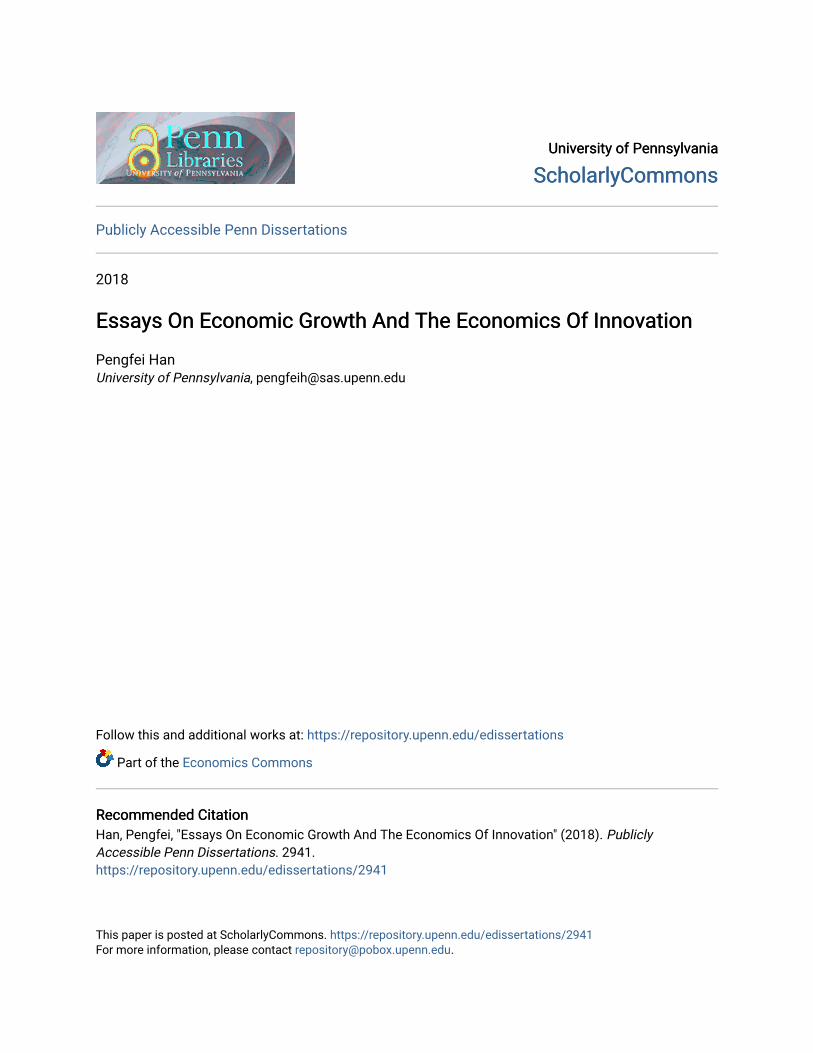
Is the actual patent law enforcement optimal? To address this issue, the optimal strength of
1The strength of patent rights is measured by the likelihood for a patent to be invalidated by the court.When a patent is involved in litigation, it can be adjudicated to be valid or invalid by the court. If a patentis less likely to be invalidated, the implied patent rights are stronger.
4

patent rights is characterized by quantitative analysis, and it is contrasted with the actual
patent law enforcement in practice. Through the lends of the model, the pro-patent legal
reform in 1982 was welfare-enhancing, but it was too extreme. Swinging back the legal
pendulum and weakening patent rights can improve welfare.
Relationship to the Literature. This paper contributes to two branches of literature:
the theory of the firm and the optimal strength of patent rights.
The theory of the firm originates from Coase (1937). In this seminal paper, Coase con-
ceptualizes a trade-off between “transaction costs” and “coordination costs” for the firm
boundary decision. Hence, the firms exist to internalize the “transaction costs.” Though
studies in this field halted for several decades, it was revived by Williamson (1971) and has
become a fertile field since then. Williamson (1971) attributes the “transaction costs” to
socially inefficient “haggling” for “appropriable quasi-rents.” A classic example is the Gen-
eral Motors – Fisher Body relationship, as analyzed by Klein (1988, 2000b). This insight
has triggered a large empirical literature on “transaction costs economics,” such as Mon-
teverde and Teece (1982), Anderson and Schmittlein (1984), Masten (1984), and Joskow
(1985). This literature, however, focuses on the benefits of integration and is largely silent
on its costs. In contrast, an alternative approach is taken in the “property-rights theory”
pioneered by Grossman and Hart (1986), Hart and Moore (1990), and Hart (1995). In this
literature, bargaining is efficient, and, thus, the parties in a contract can share the surplus
from their investment via bargaining. A larger share of asset ownership implies larger share
of the surplus, and, hence, stronger incentive to invest. In this framework, one party in
a contract should own all the assets if it is socially optimal to maximize the investment
of this party. On the other hand, the asset ownership should be divided if the investment
incentives for both parties are important. In both approaches (i.e., the “transaction costs
economics” and “property-rights theory”), the source of “transaction costs” is the hold-up
problem in various forms. In contrast, the “transaction costs” in this paper originate from
5

the infringement problem (i.e., firms may infringe on each others’ intellectual property).
This is a unique problem for the innovating sectors, because the core assets of the innovat-
ing firms are intellectual property. This insight entails special consideration for the business
scope decisions in the innovating sectors.
As epitomized in Arrow (1962), there is a classic trade-off for the optimal strength of patent
rights: stronger patent rights encourage R&D, but spur monopoly pricing by patent owners.
This is reminiscent in Tirole (1988), Romer (1990), Grossman and Helpman (1991), and
Aghion and Howitt (1992). Based on this trade-off, one branch of this literature studies
the optimal length and breadth of patent protection. In Klemperer (1990) and Gilbert and
Shapiro (1990), the optimal patent protection features long duration to encourage R&D,
but a narrow breadth to discourage monopoly pricing. Acemoglu and Akcigit (2012) studies
the state-dependent policy and proposes a “trickle-down” optimal patent protection scheme
(i.e., greater protection to technology leaders that are further ahead than those that are
close to their followers). The second branch of this literature follows a mechanism design
approach for the optimal strength of patent rights. As a classic example, Scotchmer (1999)
characterized the patent renewal system as an optimal mechanism when the quality and
costs of projects are unknown. Llobet, Hopenhayn and Mitchell (2006) study optimal patent
policy with sequential innovation and heterogeneous quality. None of these papers considers
the impact of patent rights on firms’ business scope decisions. This gap is filled in this
paper. As demonstrated in this paper, firms shrink their scope of business and specialize,
in response to stronger patent rights. This enhances firm performance and constitutes an
additional benefit of patent rights. Hence, the optimal patent rights will be stronger when
its impact on firm boundaries is taken into account.
The rest of the paper is organized as follows. Section 1.2 reviews the background of patent
law enforcement and specialization in the innovating sectors. The model is built in section
1.3 and matched with the stylized facts in section 1.4. The implications of the model are
derived by the quantitative analysis in section 1.4, and these implications are tested by the
6

empirical analysis in section 1.5. The optimal strength of patent rights is characterized in
section 1.6, and it is compared with the actual patent law enforcement in practice. Section
1.7 concludes.
1.2. Background
1.2.1. Patent Law Enforcement
As the first step to investigate the impact of patent law enforcement on specialization, this
section outlines the legal background of patent litigation in the United States. In particular,
this section highlights how a major legal reform during the 1980s created a more pro-patent
legal environment.
Patent Litigation Process
The intellectual property rights of an invention are embodied in a patent, which provides
the potential (but not the guarantee) to exclude others from using the patented technology.
In the United States, patents are granted at the United States Patent and Trademark Office
(USPTO). In contrast, the patent law is interpreted and enforced via the court system, and
the court has a final say on the strength of the patent.
When a patentee identifies a potential infringement, she may bring the alleged violators to
the court and sue them for infringement. In response, the defendant will typically counter
sue by arguing that the patent is actually not valid in the very first place, and in consequence
the patents can be invalidated by the court2. Therefore, the fate of the patent eventually
depends on the judgment and the attitude of the court. From this perspective, the fraction
of cases in which the patents are invalidated can be a proxy of the strength of patent rights.
Based on this proxy of patent rights, the evolution of patent law enforcement in the United
2A patents can be invalidated for a variety of reasons with respect to the legal requirement of novelty andnonobviousness. For instance, Allison, Lemley, and Schwartz (2014) shows that a patent can be invalidatedbecause of no patentable subject matter (success rate: 54%), prior art requirement of section 102 (successrate: 20%), obviousness issue of section 103 (success rate: 20%), indefiniteness issue of section 112 (successrate: 17%), lack of enablement of section 112 (success rate: 13%), inadequate written description of section112 (success rate: 15%).
7

States in the post-war era is illustrated in Figure 3.
Figure 3: Patent Law Enforcement In the United States
Legal Reform In 1982
The vertical axis of Figure 3 is the fraction of cases in which the patents are invalidated by
the court, the proxy of the strength of patent rights. As shown in this figure, the patent
law enforcement in the United States has experienced dramatic changes in the last several
decades. While the legal environment in the post-war era used to be fairly stable before
1982, there was a precipitous plummet in the fraction of cases invalidating the patents
around 1982. In consequence, patent law enforcement moved to a new legal regime after
1982 with remarkably lower invalidation rate and stronger patent rights.
This change of the legal environment was due to a sweeping legal reform on the court system
in 1982. Before 1982, all patent-related cases were initiated at one of the ninety-four district
courts across the country, and the litigants may further appeal to the regional appellate
courts if they disagree with the court decisions. In practice, however, the interpretation and
enforcement of the patent law were highly inconsistent across circuit courts before 1982,
8

leading to a regionally fragmented legal system3.
To address the issue of inconsistent patent law enforcement across the nation, in 1982 the
Congress established a single appellate court to hear all the appeals of patent-related cases:
the Court of Appeals of the Federal Circuit (CAFC). After this legal reform, this new court
turned out to hold a salient pro-patent attitude. To see the impact of this legal reform,
Table 1 performs a before-and-after comparison. Reported in this table is the fraction of
cases invalidating the patents across circuit courts. A revealed in Table 1, there is a decrease
in patent invalidation in every circuit court. This indicates stronger patent rights after the
legal reform. In addition, there is a decrease in the dispersion, so the litigants are treated
more equally around the country. This implies increasing legal uniformity across the nation.
Table 1: Patent Law Enforcement
Circuit Headquarter Fraction of Cases Invalidating the Patents (%)
Before 1982 After 1982
Boston 0.68 0.22
Chicago 0.56 0.32
Cincinnati 0.60 0.28
Denver 0.42 0.16
New Orleans 0.41 0.23
New York City 0.67 0.26
Philadelphia 0.76 0.29
Richmond 0.54 0.22
San Francisco 0.59 0.29
St. Louis 0.67 0.37
Nevertheless, these changes in patent invalidation rates can be attributed to changing types
of cases brought to the court. To address this concern, Table 2 conducts a regression
analysis to examine the impact of this legal reform on patent law enforcement, controlling
3In principle the Supreme Court could step in to ensure legal uniformity across circuit courts. In practice,however, the patent-related cases were rarely heard at the Supreme Court, and, hence, the discrepancy ofpatent law enforcement across circuits persisted over the years.
9

for the characteristics of the patents and the litigants involved in the lawsuits. The unit
of observation in this regression are the individual patents reviewed by the court between
1946 and 2006. The dependent variable is a dummy for patent invalidation (which takes the
value of one if this patent is invalidated by the court), and the main explanatory variable
is a dummy for the legal reform (which takes the value of one if the court decision is made
after 1982).
As demonstrated in Table 2, a patent is more likely to be invalidated after the legal reform
in 1982, even after controlling for the characteristics of the patents and the litigants involved
in the lawsuits4. In addition, this regression also uncovers a number of patterns of patent
litigation: a patent is less likely to be invalidated when it constitutes a more important
invention (as captured by more forward citations the patent receives), and when the patent
has survived more years before being brought to the court. In contrast, it is more likely to
be invalidated when the patentee is challenged in the court as the defendant (in contrast to
the scenario where the patentee sues for infringement as the plaintiff).
The bottom line of this regression is, the same type of patent is less likely to be invalidated
after the legal reform. This is suggestive evidence for a more pro-patent legal environment
and stronger patent rights after the legal reform.
In light of these dramatic changes in the court system, the next question is, how do the the
firms respond to this changing legal environment?
4To be specific, this regression controls for the number of forward citations received by the patent (thetruncation issue is addressed following Hall, Jaffe and Trajtenberg (2001)), the age of the patent at thelawsuit, the number of claims of the patent, dummies for the technology class of the patent, dummies for thecircuit court where the final court decision is made, whether the patentee is the plaintiff or the defendant,and whether the patentee is U.S. or non-U.S. inventor.
10

Table 2: Impact of the Legal Reform On Patent Law Enforcement
1 Patent Invalidated by the Court
(1) (2) (3)
CAFC (= 1 after 1982) −0.786*** −0.743*** −0.619***
(0.0851) (0.105) (0.139)
ln(num of citations received) -0.0806**
(0.0326)
age of patent at the lawsuit -0.0184*** -0.0358**
(0.00649) (0.0151)
patentee as the defendant 0.156** 0.285**
(0.0738) (0.127)
ln(num of claims) -0.0614*** -0.0167
(0.0173) (0.0338)
foreign patentee -0.104*** 0.0466
(0.0376) (0.0681)
technology class N Y Y
circuit court N Y Y
Observations 5,172 4,043 1,234
Notes: Probit regression of patent invalidation. The control variables are the number of forward
citations received by the patent, the age of the patent at the lawsuit, the number of claims of the
patent, dummies for the technology class of the patent, dummies for the circuit court, whether the
patentee is the plaintiff or the defendant, and whether the patentee is U.S. or non-U.S. inventor. Ro-
bust standard errors in parentheses (clustered at the level of circuit court). *** denotes significance
at the 1 percent level, ** at the 5 percent level, and * at the 10 percent level.
1.2.2. Specialization In the Innovating Sectors
The dramatic change in the legal environment underlined in the last section has a far-
reaching impact on the industrial-organizational structures in the innovating sectors. To
11

uncover this impact, this section develops an empirical measure of innovation specialization
based on the technological distance of patent. As shown in this section, there is increasing
specialization in the innovating sectors in the United States in the recent decades, in the
sense that the innovators invent in more closely related technological fields. In addition, as
demonstrated in the regression analysis, this increasing innovation specialization is in part
due to strengthened patent rights.
To gauge the degree of specialization in the innovating sectors, a metric of technological
distance between patents is applied as a measure of firms’ business scope with respect their
innovating activities. The underlying rationale is, when a firm invents in more closely
related technological fields, this signals a more focused business scope strategy and a higher
level of innovation specialization.
The measure of technological distance5 follows the metric developed in Akcigit, Celik, and
Greenwood (2016). This distance metric is based on the citation links between the patents.
To be specific, the technological distance between two patent classes X and Y is defined as:
d(X,Y ) = 1− #(X ∩ Y )
#(X ∪ Y ), d(X,Y ) ∈ [0, 1].
In the expression above, d(X,Y ) is the technological distance between two patent classes
X and Y , #(X ∩Y ) is the number of patents that cite both X and Y , and #(X ∪Y ) is the
number of patents that cite either X or Y . The rationale underlying this distance metric is
straightforward: the more X and Y are cited together, the closer they are. By construction,
this measure is always between 0 and 1, and a lower distance implies the patents are closer
to each other.
5In the baseline empirical analysis, technological fields are measured at the level of 3-digit InternationalPatent Classification (IPC).
12

Figure 4: Increasing Innovation Specialization
Based on this measure, the evolution of the business scope of the average U.S. innovator
is tracked in Figure 4. The vertical axis in Figure 4 is the average technological distance
between the new patent and the existing patent portfolio of the innovators6. As revealed in
Figure 4, the average U.S. innovator is inventing in more closely related technological fields,
which implies shrinking business scope and increasing specialization in the recent decades7.
6To be specific, for each innovator in each year, the technological distance between the new patent itobtains and its existing patent portfolio at the beginning of the year is calculated. The vertical axis is theaverage technological distance across the innovators in each year.
7Echoing these findings, Chesbrough (2006) documented increasing specialization in the semiconductorand life science industry. Back in the 1960s, the semiconductor industry was dominated by only two cor-porations: IBM and AT&T. Both of them included in their operations the entire production process fromdesign to manufacturing. The landscape of this industry, however, started to change in the 1970s. Intel andTexas Instruments were created and they specialized in the production of chips, ushering in the emergingmarkets of intermediate inputs for semiconductors. By the 1980s, a revolutionary separation was introducedin the semiconductor industry, leading to a dichotomy of this industry into the “fabs”, specializing in thefabrication of semiconductors (e.g., TSMC), and the “fabless”, specializing in the design function. Thedesign tools were further stripped in the 1990s, as epitomized by Qualcomm and ARM Holdings. Both ofthem offered their intellectual property underlying the design tools and effectively created a market for thedesign itself. The specialization in the semiconductor industry was by no means a unique experience. Inthe 1970s, pharmaceutical manufacturers, such as Pfizer and Johnson and Johnson, used to keep a wholearmy of staff, from the R&D team developing new drugs to the marketing division promoting their prod-
13

1.3. Model
1.3.1. Environment
Consider an economy where time is discrete. There are 3 types of agents in this economy:
the household, the final good producer, and the intermediate goods firms. The final goods
are assembled by combining a range of intermediate goods with labor. The intermediate
goods are produced by the intermediate goods firms, and there is a constant marginal cost
of production. The source of growth in this economy is expanding varieties of intermediate
goods a la Romer (1990).
Patent
In this economy, the production technology of every intermediate input is embodied in a
patent. In addition, there are 2 types of patents: the active patents and the expired patents.
The number of active patents is N , and the owners of the active patents enjoy exclusive
rights over their intellectual property. The number of expired patents is N , and everyone
has free access to the technologies embodied in these patents. An active patent can expire
for 2 reasons. In practice, the term of the patent is limited. This is captured by stochastic
survival with probability σ. In addition, the active patents can be involved in litigation,
and they can be invalidated by the court. Once they are invalidated, they join the pool of
the expired patents. This is a crucial channel for the court system to change the landscape
of technology. Through this channel, the expired patents are introduced to capture the
impact of the legal institution.
ucts. In the 1980s, the development of new drugs began to be led by biotechnology firms specializing inthe discovery of new compounds. The pharmaceutical producers acquired the patents of the compoundsfrom these biotech firms, conducted clinical trials and then offered the new drugs to the market. Turningto the 1990s, independent research organizations specializing in performing clinical trials (e.g., MillenniumPharmaceuticals) were created, and they focused on testing the safety and efficacy of the new drugs.
14

Intermediate Goods Firm
The intermediate goods firms own all the patents, and they can produce the intermediate
goods associated with the patents they hold. The boundaries between these firms can be
identified by the range of intermediate goods they produce in-house. These intermediate
goods are produced to serve 2 types of customers. They are sold to the final goods producer
at price q, and they are used to produce the final goods. They are also sold to other
intermediate goods firms at price p, and they are used in the R&D process to discover new
varieties of intermediate goods. The prices p and q are different, because the underlying
demand functions are different, as will be shown later. There is no resale between these
2 market segments. In addition, the intermediate goods firms can discover new varieties
of intermediate goods from R&D, and they file a new patent for every new variety of
intermediate good they discover. They can keep the new patents they develop, or they can
sell them to other intermediate goods firms. They can also buy new patents, and all patents
are traded at their intrinsic value (i.e., the present value of the future payoff).
R&D: Input and Output
The R&D process in this economy is illustrated in Figure 5.
Figure 5: R&D: Setup
15

The input of R&D is a basket of the existing intermediate goods. These inputs are used
in the corporate lab to discover new varieties of intermediate goods. By investing a basket
of intermediate goods miN+Ni=0 , an intermediate goods firm can discover new varieties of
intermediate goods in the amount of G(miN+Ni=0 ) = 1
θ
∫ N+N0 (mi)
θdi.
These new varieties of intermediate goods are the output of R&D. They can be the blue
prints of new semiconductors, or they can be the chemical structure of new drugs and
medicine. The intermediate goods firms file a patent for each new variety of the intermediate
goods they discover. This is how technology advances in this economy.
R&D Inputs: Sources and Costs
Where do the R&D inputs come from? They come from 3 sources, as depicted in Figure 6.
Figure 6: R&D Inputs: Sources and Costs
For some of the intermediate goods, the underlying production technology is embodied in
the expired patents. Everyone has free access to these inputs, and they can produce them
in-house at the cost φ. In contrast, for some of the intermediate goods, the underlying
production technology is embodied in the active patents. These patents have owners. For
instance, a semiconductor has many components. Some of these components are associated
with the patents owned by Intel, and some components are based on the patents of Texas
16

Instruments. To develop a new semiconductor, Intel needs to combine the components based
on its own patents, with the components patented by Texas Instruments. For the first type
of the components, Intel can simply produce in-house, and there’s a production cost, φ. In
contrast, to obtain the components based on the patents of Texas Instruments, Intel has 2
options. He can buy these components from Texas Instruments, and he needs to pay the
price p. Alternatively, Intel can infringe on the patents of Texas Instruments, by imitating
its product and producing in-house. That is to day, Intel can produce the same component
of Texas Instruments, but their production cost can be different. The production cost of
Texas Instruments is φ, and the cost of Intel, the imitator (or the infringer), is λφ. λ is
firm-specific random variable, and it captures heterogeneous firm capabilities to imitate.
In addition, λ is uniformly distributed on [0, λ], and it is independently and identically
distributed across firms and across periods.
Legal Institution
The legal institution to resolve the disputes are outlined in Figure 5. When the patent of
an intermediate goods firm is infringed by other firms, it can sue them in the court. In
response, the alleged infringers will challenge the validity of the patent, and the court will
make a decision on whether this patent is valid or invalid. If the patent is adjudicated to
be valid, the patent owner will receive a legal settlement. If the patent is adjudicated to be
invalid, this patent will expire. In addition, a patent is more likely to be invalidated when
more firms challenge the validity of this patent in the court. In order to invalidate a patent,
the number of firms needed to challenge the patent follows an exponential distribution with
parameter τ . That is to say, when a patent is challenged by f firms, this patent will be
invalidated with probability 1− e−τf .
17

Figure 7: Legal Institution
Measure of Specialization
In this economy, the production technology of every intermediate good is embodied in a
patent. The number of patents a firm own determines the range of intermediate goods that
it produces in-house, in contrast to the intermediate goods purchased from the external
market. The model features representative firm. Every firm holds the same number of
patents: s. Hence, the number of intermediate goods a firm produces in-house is also s.
The business scope of the firm can be captured by s, because s pins down the boundary
between the intermediate goods produced in-house, and the intermediate goods purchased
from the external market.
In addition, the level of integration of the firm is captured by sN , the fraction of intermediate
goods the firm produces in-house. An increase in sN implies a higher level of integration,
and a lower level of specialization. s is a key choice of the firm8, and the number of the
firms, F , is pinned down by Ns . The number of the firms will settle down along the balanced
growth path.
Management Costs
It is costly to manage the business in this economy. To be specific, the management cost
for a firm is Ω( sN , w) = 1ξ+1
(sN
)ξ+1w. The management cost is increasing in the wage rate,
8More precisely speaking, s is a key state variable of the firm. Every firm starts with s at the beginningof the period, and it chooses s′ for the next period.
18

w. Imagine every firm needs to hire managers to run the business. In addition, another key
factor in the management cost is sN , the fraction of intermediate goods the firm produces
in-house. The management cost is increasing and convex in sN . Imagine the management
monitoring is subject to diminishing return to scope. The convexity of Ω implies scope
diseconomies and benefits of specialization. When a firm pursues a more focused business
strategy with lower sN , the firm can enhance its management efficiency because of the
convexity of the management cost function. The degree of scope diseconomies and the
benefit of specialization is governed by the magnitude of the convexity (ξ).
Timing of Events
As bird view of the major decisions of the intermediate goods firms, the timing of events is
illustrated in Figure 8. At the beginning of the period, the production cost under imitation
(λ) is realized. Based on their λ, the firms will decide whether to buy the intermediate goods
from other firms or infringe on their patents. Then the firms will produce the intermediate
goods, and decides how much to spend in R&D. The legal disputes will be settled in the
court, and the firms will make payment to each other based on the court decisions. If a
firm’s patents are infringed and it wins the lawsuit, this firm will receive a legal settlement
from the violator. Meanwhile, if a firm infringes on others’ patent and loses the case, it will
have to pay the compensation to the patentee. Lastly, the firms can trade patents before
the end of the period, so that every firm can adjust its business scope to any level as it
desires.
Based on this setup, the decisions of the agents are delineated as follows.
19

Figure 8: Timing of Events
1.3.2. Households
There is a representative household in this economy. The household is endowed with one unit
of labor. Labor supply of the household is inelastic. The household owns all the firms and
earns income from wages and the dividends collected from the firms. The objective of the
household is to maximize the lifetime utility with discount rate β for future. The preference
of the household is characterized by CRRA utility with momentary utility function: U(c) =
c1−ε
1−ε , where c refers to current consumption and ε is the coefficient of relative risk aversion.
Since this setup is entirely standard, the household problem is not explicitly delineated.
1.3.3. Final Goods Producer
The final goods in this economy are assembled by combining labor with a range of interme-
diate inputs. To be specific, the final goods are produced under the following production
technology:
Y =1
α
∫ N+N
0xαi di L
1−α
In this production function, L is the labor input and 1 − α is the share of labor. xi is the
quantity of intermediate input i, and the varieties of the intermediate inputs are ranging
from [0, N+N ]. Recall N and N are the number of active and expired patents, respectively,
20

and N + N is the total number of intermediate inputs (or patents). There is a constant
marginal production cost φ for the intermediate inputs based on the expired patents (i.e.,
i ∈ [0, N ]). For the intermediate inputs associated with the active patents (i.e., i ∈ [0, N ]),
the final goods producer is facing a price q charged by the owner of the active patents.
Therefore, the final goods producer is facing the problem:
maxxiN+N
0 , L
1
α
∫ N+N
0xαi di L
1−α −∫ N
0q xidi−
∫ N+N
Nφ xidi− wL
The first term in the problem of the final goods producer is the output, the second term
is the expenditures on the intermediate inputs associated with active patents, the third
term is the production cost for intermediate inputs associated with expired patents, and
the last term is the labor cost. The problem of the final goods producer delivers the demand
function q(xi) for the intermediate input associated with active patent i and the wage rate
of labor9.
1.3.4. Intermediate Goods Firms
The intermediate goods firms are the core players in this economy, and their decisions are
delineated in this section.
Buy or Infringe?
To begin with, an intermediate goods firm is facing the following decision: to obtain the
intermediate goods associated with others’ patents, should it buy their products or infringe
on their patents? The key determinant for the decisions to buy or infringe is the firm’s
production cost under imitation (λ). A firm can enjoy lower R&D cost if it decides to
infringe on others’ patent, because it can imitate their product and produce in-house, instead
of buying their product from the market. On the other hand, an infringer may lose the
lawsuit when being sued in the court. In consequence, the infringer will have to pay the
9Recall there is an inelastic supply of labor with one unit.
21

legal settlement. From this perspective, an infringer is facing the trade-off between lower
R&D cost versus paying a legal settlement when losing the lawsuit. In equilibrium, the firms
will follow a cutoff strategy to infringe (i.e., a firm will infringe if and only if its imitation
cost λ is below a threshold)10. This threshold for the infringement decision will be precisely
pinned down later in the section of equilibrium characterization.
Operating Profits
An intermediate goods firm can produce the intermediate goods associated with its patent,
and sell them to both the final goods producer and other intermediate goods.
To be specific, the price an intermediate goods firm sets for the final goods producer is
determined in the following problem:
πX = maxq, x
(q − φ)X(q)
s.t. X(q) : demand of final goods producers
An intermediate goods firm seeks to maximize the profits obtained from the final goods
producer, and the equilibrium operating profit is denoted by πX . There is a constant
marginal production cost φ for the intermediate inputs based on the active patents (i.e.,
i ∈ [0, N ]). q is the price the intermediate goods firm chooses to charge the final goods
producer, X(q) is the quantity demanded by the final goods producer given the price q.
In addition, the intermediate goods firms also need the products of each other, because
these intermediate inputs will be used for R&D. Each firm has two options to access to
the inputs based on others’ patents: it can buy their products, or infringe on their patents
by imitating their products. The decisions of other firms to buy or infringe depend on the
price charged by the intermediate goods firm. To be specific, the price p a patent holder
10Recall the imitation cost λ is a firm-specific variable. Hence, when a firm decides to infringe, it infringeson everything outside her own patent portfolio.
22

charges other patent holders is determined as follows:
πM = maxp, m
(p− φ)×M(p)× (1− λ)F
s.t. M(p) : demand of other patent holder
s.t. λ(p) : fraction of firms that infringes
An intermediate goods firm seeks to maximize the profits obtained from other intermediate
goods firms, and the equilibrium operating profit is denoted by πM . In the expression above,
p is the price the intermediate goods firm charges, and M(p) is the quantity demanded given
the price p. The demand function M(p) hinges on the return from R&D. Given the price p
set by an intermediate goods firm, a fraction 1− λ of the firms will buy her products, and a
fraction λ of the firms will infringe on her patent. Hence, the number of buyers is (1− λ)F
, where F is the total number of intermediate goods firms in this economy. As will be
shown later, λ is increasing in p, the price charged by the intermediate goods firm. Hence,
when a firm charges a lower price, more people will decide to buy its products instead of
infringing. In addition, λ is increasing in τ , the odds for the patent to be invalidated by
the court. When the patents are more likely to be invalidated, more firms will decide to
infringe instead of buying. This is a crucial channel for the court system to change the firm
decisions.
Patent Survival Rate
In this economy, a patent may expire for two reasons. First, the term of the patent is limited
and this is captured by stochastic survival with probability σ.11 In addition, a patent can
be involved in litigation when it is infringed, and the patent may be invalidated when being
challenged in the court. The number of alleged infringers challenging the patent is λF , so
11In the quantitative analysis, σ will be specified to match the term of the patent in practice.
23

the patent will be adjudicated to be valid 12 with probability e−τλF . Hence, the survival
rate of patent is η = σe−τλF .
Legal Settlement Received
Though the intermediate goods firm does not receive any payment from the infringers, it can
bring them to the court and sue them for infringement. In each lawsuit, the patent owner can
win and receive the legal settlement with probability e−τλF . The amount of the settlement
upon victory is a fraction µ of the price of the patent, P .13 However, it is costly to sue
people, and the cost of litigation is a fraction ψ of the price of the patent, P . Hence, the net
legal settlement received by an intermediate good firm is z×s = (e−τλFµP −ψP )× λF ×s.
Patent Trading
At the end of the period, all firms can adjust their business scope to any level as they
desire. This adjustment can be achieved by trading their patents with each other. There is
a centralized market for patent trading, where every patent can be traded at the intrinsic
value (i.e., the present value of the future payoff). To be specific, the price of the patent is:
Pt =
∞∑j=0
ηj (πt+j + zt+j)
Rj
The price of a patent at period t is denoted by Pt.14 The price of a patent is the present
value of the expected payoff in future, and the future payoffs of a patent is discounted
by the gross interest rate, R. In each period, the patent can survive with probability η.
Conditional on survival, there are two sources of income for a patent: operating profits
collected from the buyers (π) and legal settlement received from the infringers (z).
12In order to invalidate a patent, the number of firms needed to challenge the patent follows an exponentialdistribution with parameter τ . That is to say, when a patent is challenged by f firms, this patent will beinvalidated with probability 1− e−τf .
13The value of the patent (P ) will be delineated momentarily in the next section.14The price of patent will settle down along the balanced growth path.
24

Given the price P ′, every firm chooses the number of patents to trade, h, and its expenditure
on patent purchase (or revenue from patent sale) is H = hP ′. A positive choice of h implies
patent purchase, and a negative choice of h implies patent sale.
Value Function
Combining the payoffs of the patent holders delineated in the previous sections, the value
function of the intermediate goods firm is characterized as follows:
V (s;N, N ;λ) = max Buy (B), Infringe (I)
V B(s;N, N), V I(s;N, N ;λ)
There are four state variables for the intermediate goods firm: the number of patents it
owns (s), its production cost under imitation (λ), the total number of active patents (N),
and the total number of expired patents (N). In addition, every intermediate goods firm
is facing two states of the world: she can be a buyer if she decides to buy the products of
other intermediate goods firms, or she can be an infringer if she infringes on others’ patent
by imitating their products and producing in-house.
If an intermediate goods firm decides to buy the products of other firms, its value function
is characterized as follows:
V B(s;N, N) =
maxq, p, miN+N
i=0 ,h,s′
πX(q)× s+ πM (p)× s+ z × s− I(miN+N
i=0
)− h× P ′
−Ω( sN , w) + 1REλV (s′;N ′, N ′;λ′)
s.t. s′ = ηs+G
(miN+N
i=0
)+ h
There are four choices of the intermediate goods firm: the price it charges the final goods
producer (q), and the price it charges other intermediate goods firms (p), how much it spends
on R&D (miN+Ni=0 ), and how many patents to buy or sell (h). The current payoff of the
25

intermediate goods firm is its operating profits obtained from producing the intermediate
goods (πX(q)×s+πM (p)×s), plus the legal settlement received for being infringed (z×s),
minus its R&D expenditures (I(miN+N
i=0
)), minus its purchase or sale of patents (h×P ′),
minus its management costs (Ω( sN , w)). The law of motion for the number of patents a firm
has is: s′ = ηs+G(miN+N
i=0
)+ h. At the beginning of the period, every firm starts with
the same number of patents, s, and a fraction η of the patents can survive. There will be
new patent developed from R&D, G(miN+N
i=0
). At the end of the period, the firm can
choose the number of patents to trade, h.
Analogously, if an intermediate goods firm decides to infringe, its value function is charac-
terized as follows:
V I(s, λ,N, N) =
maxq, p, miN+N
i=0 ,h,s′
πX(q)× s+ πM (p)× s+ z × s− I(miN+N
i=0 , λ)− h× P ′
−∆− Ω( sN , w) + 1REλV (s′;N ′, N ′;λ′)
s.t. s′ = ηs+G
(miN+N
i=0
)+ h
When an intermediate goods firm decides to infringe, it imitates others’ products and pro-
duces them in-house. Because of this, its R&D expenditures depend on its imitation cost,
λ. On the other hand, it has to pay the legal settlement (∆) if it loses the lawsuit in the
court.
The key determinant for the decisions to buy or infringe is the firm’s production cost under
imitation (λ). This decision is static because λ is independently and identically distributed
across periods. In addition, the optimal pricing and R&D decisions are designed to be static
in this model, so the only dynamic choice is s′, the choice for the scope of business in the
next period. In equilibrium, every firm will choose the same s′, because every firm has the
26

same marginal cost15 and the same marginal benefit 16 of holding one more patent in the
next period.
1.3.5. Equilibrium
Cutoff Strategy to Infringe
As revealed in the previous discussion, the key determinant for the decisions to buy or
infringe is the firm’s production cost under imitation (λ). Given λ, a potential infringer is
facing the trade-off between lower R&D cost and paying a legal settlement when losing the
lawsuit. In equilibrium the firms will follow a cutoff strategy to infringe in the following
form:
Proposition 1. (Cutoff Strategies to Infringe) A firm infringes if and only if its production
cost under imitation λ ≤ λ, where λ is determined by V I(s;N, N ; λ) = V B(s;N, N).
Conditional on the decision to buy, the value function of the firm no longer depends on
its production cost under imitation (λ). In contrast, the value function of the infringer
is strictly decreasing in its λ. Therefore, in equilibrium a firm infringes if and only if its
production cost under imitation (λ) is lower than λ, and the threshold λ is determined where
the value function of the buying coincides with the value function of infringing. Since λ is
uniformly distributed on [0, λ], the fraction of firms that infringes is λ =λ
λ.
Balanced Growth Path
Proposition 2. (Balanced Growth Path) There exists a balanced growth path17 along
which:
15The marginal cost of holding one more patent is P ′, and every firm is facing the same price.16The marginal benefit of holding a patent is how much a firm expects her payoff can be boosted by
holding one more patent in the next period, and this expected boost in payoff depends on whether shebuys or infringes in the next period. In addition, since λ is i.i.d. across periods, every firm has the sameexpectation for the next period, and this does not depend on the current status of buying and infringing, sothe marginal benefit of holding one more patent is the same for every firm.
17The balanced growth path can be solved by five variables from five equations. The five variables are:the price set for other intermediate goods producer, the cutoff of imitation cost to infringe, the price of thepatent, the number of the firms, and the growth rate of the number of active patents.
27

1. The number of the firms (F ) is constant.
2. The number of active patents (N) and expired patents (N) grow at the same rate.
3. Output (Y ) , comsumption (c) , wages (w) , and the number of patents held by each
firm (s) all grow at the same rate as the number of active patents (N).
1.4. Quantitative Analysis
The theoretical model established in the previous section offers an apparatus to conduct
thought experiments and policy evaluations. To achieve this objective, the parameters of
this model are calibrated to match the data in this section. The quantitative analysis delivers
three major implications of the model: (1) stronger patent rights induce specialization, (2)
specialization enhances firm performance, and (3) specialization contributes to economic
growth.
1.4.1. Calibration
The value of the parameters in this model are reported in Table 3. These parameters fall
into three groups: parameters underlying the preferences of the households, parameters
governing the technology of production and R&D, and parameters characterizing the legal
system.
Seven of these parameters are determined by a priori information, and the detailed identi-
fication strategies are delineated as follows.
1. CRRA parameter for households, ε. The CRRA parameter is determined by taking
the average values of the estimates in Kaplow (2005).
2. Long-run interest rate, R. The long-run interest rate in the United States follows
Cooley and Prescott (1995).
3. Discount factor for households, β. The discount factor for households is deduced from
the interest rate (R), the CRRA parameter for households (ε), and the growth rate
28

of the economy18.
4. Capital share, α. The capital share is based on the U.S. National Income and Product
Accounts, as reported in Corrado, Hulton and Sichel (2009).
5. Imitation cost, λ. The imitation cost is gathered from Mansfield, Schwartz, and
Wagner (1981).
6. Patent survival rate, σ. The term of patents in the United States is 17 years, so σ is
taken to be 11/(1 + 17).
7. Litigation cost, ψ. The litigation cost is based on the report of the American Intellec-
tual Property Law Association (2011)19.
The other six parameters, φ (production cost of intermediate inputs associated with the ac-
tive patent), φ (production cost of intermediate inputs associated with the expired patent),
θ (degree of complementarities in R&D), ξ (convexity of the management cost), τ (pa-
rameter for the odds to invalidate a patent) and µ ( legal settlement for infringement) are
calibrated to match five data targets. The model moments are contrasted with the data
targets in Table 4. The sources of the data targets are discussed as follows.
1. Level of integration. This is the average fraction of technological field20 a firm invents
in between 1982 and 2006. The patenting information is obtained from the NBER
patent dataset project.
2. Ratio of expenditure on R&D inputs purchased from the market to in-house R&D.
This is the ratio of royalties to R&D taken from the report of the National Science
Foundation (2013).21
18To be specific, the discount factor for households (β) is pinned down from the Euler equation of thehouseholds.
19As reported by the American Intellectual Property Law Association, the average litigation cost is 2.8million dollars when the value at risk is between 1 million and 25 million dollars.
20The technological fields are measured at the level of 3-digit International Patent Classification (IPC).21More details can be found in Shackelford (2013).
29

3. Fraction of cases invalidating the patents. This is based on the records of the United
States Patents Quarterly (USPQ).
4. Litigation cost to R&D ratio. The ratio of litigation cost to R&D is gathered from
Lerner (1995).
5. R&D expenditures to GDP ratio. The ratio of R&D expenditures to GDP is calculated
from the U.S. National Income and Product Accounts.
6. Growth of real GDP per capita. This is the average growth rate of real GDP per
capita between 1982 and 2006, as calculated from the U.S. National Income and
Product Accounts.
Table 3: Parameter Values
Parameter Value Description Identification
β 0.98 discount factor for households A priori information
ε 2.00 CRRA parameter for households A priori information
R 0.06 interest rate A priori information
α 0.60 capital share A priori information
φ 140 production cost for intermediate goods Calibration
associated with active patents
φ 110 production cost for intermediate goods Calibration
associated with expired patents
θ 0.44 concavity of inputs in R&D function Calibration
λ 1.30 imitation cost A priori information
ξ 2.71 convexity of management cost function Calibration
σ 0.94 patent survival rate A priori information
τ 0.61 parameter for the odds to invalidate a patent Calibration
ψ 0.21 litigation cost A priori information
µ 0.68 legal settlement for infringement Calibration
30

Table 4: Calibration Target
Target Source Model (%) Data (%)
level of integration ( sN ) USPTO 1.4 1.4
ratio of expenditure on R&D inputs purchased NSF 13.0 13.0
from the market to in-house R&D
fraction of cases invalidating the patents US Patents Quarterly 29.0 29.0
litigation cost to R&D ratio Lerner (1995) 27.0 27.0
R&D to GDP ratio NIPA 3.3 2.9
growth of real GDP per capita NIPA 2.1 2.1
1.4.2. Stronger Patent Rights Induce Specialization
The impact of patent rights on firm boundaries is depicted in Figure 9. The horizontal
axis of Figure 9 are the odds for the patent to be invalidated by the court, a proxy for the
strength of patent rights. The dashed line in Figure 9 is the fraction of firms that infringe
on others’ patents, and the solid line is the fraction of intermediate goods the firm produces
in-house.
The scope of business is captured by the fraction of intermediate goods the firm produces
in-house, as shown on the left vertical axis of Figure 9. As revealed in this figure, when
the patents are more likely to be invalidated by the court, a higher fraction of the firms
will decide to infringe on others’ patents instead of buying their products. In response, the
firms will expand their business scope and produce a higher fraction of the intermediate
goods in-house.
This is because a major benefit of broader business scope in this model is to fend off potential
infringement. The expansion of business scope is achieved by merger and acquisition. After
acquiring some suppliers and customers, a firm will be facing a smaller number of trading
partners. The firm is less likely to be infringed, because the odds to be infringed are
increasing in the number of trading partners the firm deals with. In this way, a firm can
31

fend off infringement by expanding its business scope and acquiring its trading partners. In
the extreme, imagine a firm acquires all the patents of all the other firms, then there would
be a single firm in this economy. All the transactions will be internalized and there will
be no issues of infringement. From this perspective, when a firm is concerned about being
infringed, it can expand its business scope to fend off potential infringement and litigation.
Figure 9: Patent Rights and Firm Boundaries
In addition, this benefit is increasing in the odds for the patent to be invalidated. This is
because the patents of a firm are more likely to be infringed and invalidated with weaker
patent rights. Hence, the consequences of infringement and litigation are more severe, and
the benefit of expanding the business scope to fend off infringement increases. Therefore,
weaker patent rights can discourage specialization and stronger patent rights can induce
specialization.
32

1.4.3. Specialization Enhances Firm Performance
Figure 10 evaluates how the business scope decision of a firm affects its performance. The
horizontal axis in Figure 10 is the fraction of intermediate goods each firm produces in-house.
A higher fraction of intermediate goods produced in-house implies a broader business scope.
The dashed line in Figure 10 is the ratio of management costs to sales, and the solid line is
the marginal boost of patents to firm value.
Figure 10: Specialization and Firm Performance
As demonstrated in Figure 10, broader business scope leads to higher management costs.
Increasing costs originate from the convexity of the management costs function with respect
to the fraction of intermediate goods the firm produces in-house. In consequence, the
marginal boost of patents is increasingly lower when a firm has a broader business scope.
Hence, specialization enhances firm performance by improving firms’ management efficiency.
33

1.4.4. Specialization Contributes to Economic Growth
Figure 11 examines the relationship between specialization and economic growth. The
horizontal axis in Figure 11 is the fraction of intermediate goods each firm produces in-
house. The dashed line in Figure 11 is the ratio of R&D to GDP, and the solid line is the
growth rate of GDP per capita.
Figure 11: Specialization and Economic Growth
As shown in Figure 11, when the firms pursue a more focused business scope strategy
by producing a lower fraction of intermediate goods in-house, the economy will experience
faster economic growth. When each firm produces a lower fraction of intermediate goods in-
house, there will be a higher number of firms in this economy, each pursuing a more focused
business scope strategy with a narrower business scope. Each firm faces more buyers for its
products, and its patents generate more revenue. Hence, the patents become more valuable,
and the firms have stronger R&D incentives to develop more patents. As demonstrated in
Figure 11, the economy features higher ratio of R&D to GDP, and, thus, it grows faster.
34

1.5. Empirical Evidence
As highlighted in the previous section, the model delivers three major implications: (1)
stronger patent rights induce specialization, (2) specialization enhances firm performance,
and (3) specialization contributes to economic growth. These implications are tested by the
empirical analysis in this section.
1.5.1. Business Scope and Technological Distance
In the empirical analysis, the business scope of the firm is measured as the technological
distance between the new patents the firm develops to the existing patent portfolio of the
firm. Figure 12 illustrates how this notion of technological distance is mapped into the
model. Every firm has s patents in the model. These existing patents of the firm are
indexed from 0 to s. In addition, imagine the firm develops new patents in the amount of
ε. These new patents are indexed from s to s + ε. Define the distance between 2 patents
i and j, as the difference between their indices in absolute value, i.e., d(i, j) = |i − j|. In
this scenario, the average distance of new patents to the firms’ existing patent portfolio is
s+ ε
2.22. Hence, the new patents will be more far away from the existing patent portfolio
of the firm, when the firm has a larger business scope, s. This is how the notion of business
scope in the empirical analysis and the model are connected with each other.
Figure 12: Business Scope and Technological Distance
22To be specific, for each new patent i ∈ (s, s+ε], the distance of patent i to firm’s existing patent portfolio
is
∫ sj=0
d(i, j)dj
s= i − s
2Hence, The average distance of new patents to firm’s existing patent portfolio is∫ s+ε
i=s(i− s
2)di
ε=s+ ε
2.
35

1.5.2. Stronger Patent Rights Induce Specialization
As outlined in the introduction section, the recent decades have witnessed both stronger
patent rights and increasing innovation specialization over time. Are they related to each
other? To address this question, this section conducts a regression analysis to test the
hypothesis that stronger patent rights can induce specialization.
To begin with, the impact of patent rights can be different across firms. To the extent the
patent rights has an effect on the business scope decisions of the firms, this effect should
be stronger for firms facing higher exposure to patent litigation. Based on this idea, the
regression analysis is designed as follows.
yi,j,t = α invalidation rate j,t + β invalidation rate j,t × litigation exposure i,t +Xi,j,tδ + εi,t
This regression is based on the U.S. public firms between 1976 and 2006. The dependent
variable is the technological distance of the new patents a firm obtains in each year, to the
existing patent portfolio of the firm at the beginning of the year. To be more specific, yi,j,t is
the technological distance of the new patent to existing patent portfolio of firm i located in
circuit court j. The main explanatory variable in this regression is the “invalidation rate”,
and it refers to the fraction of cases invalidating the patents in the circuit court where
the firm is located. This is a proxy for the strength of patent rights in the firm’s local
environment.23
In addition, to capture potential heterogeneous effect across firms, there is an interaction
term between the patent invalidation rate and the exposure to litigation at the firm level
(i.e., “litigation exposure”). The measure of patent litigation exposure follows Mezzanotti
(2017). As shown in Mezzanotti (2017), firms are facing different risks to litigation because
they are inventing in different technological fields with different intensities of litigation.
From this perspective, the litigation intensity of a technological class is measured as the
23This patent invalidation rate varies both within a circuit over time, and across the circuits at each pointin time.
36

fraction of patents litigated in this class.24 Based on this measure of litigation intensity, the
exposure to litigation at the firm level is the weighted average of the litigation intensities
of all the technological classes the firm invents in, and the weight is the share of the firms’
patents in each technological class.
Xi,j,t refers to the control variables in this regression. To be specific, this regression controls
for firm employment, firm age (and age squared), the patent stock of the firm (with quality
adjustment),25 year trend, industry effect, circuit court effect, and firm fixed effect.
Table 5: Patent Rights and Specialization
ln(Tech Distance)
OLS IV
(1) (2) (3)
ln(invalidation rate) 0.0121** 0.0738*** 0.386***
(0.00516) (0.0232) (0.0648)
ln(invalidation rate) × ln(litigation exposure) 0.0166*** 0.0919***
(0.00609) (0.0155)
Observations 17,547 17,547 17,547
R-squared 0.6377 0.6379
Notes: Compustat, firm-level regressions. The control variables are firm employment, firm age (and
age squared), the patent stock of the firm (with quality adjustment), year trend, industry effect,
circuit court effect, and firm fixed effect. Standard errors are in parentheses. *** denotes significance
at the 1 percent level, ** at the 5 percent level, and * at the 10 percent level. The IV is a dummy
variable for the legal reform in 1982, which takes the value of 1 after 1982.
Based on this setup, the regression results are presented in Table 5. As shown on the first
row of Table 5, the estimate of the regression coefficient of the patent invalidation rate
is positive. Hence, when the patents are less likely to be invalidated in a circuit court,
24In the baseline empirical analysis, technological fields are measured at the level of 3-digit InternationalPatent Classification (IPC).
25Quality adjustment of patent is performed by weighting the patent counts by the number of citationsthe patent receive, and the truncation issue is addressed following Hall, Jaffe and Trajtenberg (2001).
37

firms located in this circuit tend to innovate in more closely related technological fields. In
addition, the estimate of the regression coefficient of the interaction term is also positive, so
the impact of patent rights is more pronounced for firms facing higher exposure to patent
litigation. To address potential endogeneity issues, the instrument variable (IV) approach
is adopted in the last column of Table 5. The IV is a dummy variable for the legal reform
in 1982, which takes the value of 1 after 1982. As shown in the last column of Table 5,
the conclusions are robust in this IV regression. Therefore, these regressions support the
hypothesis that stronger patent rights can induce innovation specialization.
1.5.3. Specialization Enhances Firm Performance
Does it matter for the firms to have a broad or narrow business scope? It does matter. It
matters at the firm level because the business scope strategy is key to the fate of the firm,
and it matters at the country level because of its impact on the economic growth of nations.
A telling example is the rise and fall of Yahoo. Yahoo was already a giant in both search
engine and e-commerce when Google and e-Bay were still fledging start-ups. However,
Yahoo has never been clear in where it should focus. Gradually it was defeated by Google
in search engine, and it was dwarfed by e-Bay in e-commerce. Yahoo is not alone, and the
story of Yahoo is echoed in the regression in Table 6. This regression is based on the U.S.
public firms between 1976 and 2006, and it evaluates the impact of specialization on firm
performance along three dimensions: the number of patents obtained per R&D dollar, the
TFP of the firm,26 and its market value.
Regression (1) is a patent production function, where the input is R&D of a firm and the
output is patent that the firm obtains. To capture the impact of specialization on the R&D
productivity of the firm, an interaction term between firm R&D and “technological distance”
is introduced in regression (1). “Technological distance” here refers to the technological
distance of the new patents a firm obtains each year, with its existing patent portfolio at
the beginning of the year. As shown in the second row of regression (1), the interaction
26The TFP estimation is based on Levinsohn and Petrin (2003).
38

term between R&D and technological distance has a negative regression coefficient. Hence,
a firm will harvest more patents from the same R&D dollar when it invents in technological
fields that are closer to its existing patent portfolio.
Table 6: Specialization and Firm Performance
ln(patent, quality adj.) ln(TFP) ln(market value)
(1) (2) (3)
ln(R&D) 0.186***
(0.0139)
ln(R&D) × ln(tech distance) −0.0163***
(0.00529)
ln(patent stock) 0.812*** 0.0823*** 0.105***
(0.0104) (0.0228) (0.0195)
ln(patent stock, dist-adj.) −0.0376** −0.0833***
(0.0191) (0.0167)
Observations 22,214 7,222 25,590
R-squared 0.804 0.951 0.918
Notes: Compustat, firm-level regressions. The control variables are firm employment, firm age (and
age squared), the patent stock of the firm (with quality adjustment), year effect, industry effect, and
firm fixed effect. Standard errors are in parentheses. *** denotes significance at the 1 percent level,
** at the 5 percent level, and * at the 10 percent level.
Regression (2) and (3) assess the relationship between the firms’ patent stock and their
TFP and market value. As shown in regression (2) and (3), while the patent stock has
a positive contribution to firm TFP and market value, the distance-adjusted patent stock
has a negative contribution.27 Therefore, the patent will have a stronger boost to TFP and
market value when a firm invents in more closely related technological fields. The ratio
of the second regression coefficient to the first one in regression (2) and (3) captures the
loss of larger technological distance, or, the gain of a more focused strategy. The bottom
27When constructing the distance-adjusted patent stock, every patent is weighed by its distance to theexisting patent portfolio of the firm when this patent is developed. The setup of regression (2) and (3)follows Akcigit, Celik, and Greenwood (2016).
39

line of Table 6 is that innovation specialization (or a more focused business scope strategy)
enhances firm performance, and it is embraced by the shareholders.
1.5.4. Specialization Contributes to Growth
Built on the firm-level evidence, this section extends the analysis to a cross-country study.
To evaluate the impact of innovation specialization on economic growth, a cross-country
panel regression is conducted and the results are presented in Table 7.
The regression in Table 7 covers 88 countries between 1987 and 2006. These countries
account for 98% of world GDP during this sampling period. This 2-decade sample is divided
into 4 periods, each lasting for 5 years. The dependent variable in this regression is the
average growth rate of each country in each period, and the main explanatory variable is
the average technological distance between new patents and the existing patent portfolio of
the innovators in each country in each period.28 The regression in Table 7 controls for the 2
main factors demonstrated to be important in the empirical literature: the initial GDP per
capita, and the Barro and Lee (2013) human capital index at the beginning of each period.
Since the propensity of the innovators in a country to patent in the U.S. can depend on its
trade relation with the U.S., the export to the U.S. and the import from the U.S. of each
country are included as control variables. In addition, country dummies are added in this
regression to control for country fixed effect, and period dummies are included to control
for the global aggregate shocks to all countries.
An IV regression is performed to address potential endogeneity issues. The IV is the average
technological distance between new patents and existing patent portfolio of the innovators
for each country in the pre-sampling period,29 following the strategy pioneered in Barro
and Lee (1994). The pre-sampling period is one period before the sample starts (i.e., from
1982 to 1986).
28To be specific, for each innovator in each country in each year, the technological distance between thenew patent it obtains and its existing patent portfolio at the beginning of the year is calculated. Theexplanatory variable in this regression is the average technological distance across the innovators in eachcountry in each period.
29The country dummies have to be dropped because the IV is country-specific and time-invariant.
40

Table 7: Specialization Contributes to Growth
growth of GDP per capita
OLS IV
(1) (2)
tech distance −4.548** −5.692*
(2.062) (3.361)
Observations 267 185
R-squared 0.531
Notes: Country-level regressions. The control variables are the initial GDP per capita and the Barro
and Lee (2013) human capital index, the export to the U.S. and the import from the U.S. of each
country, the country dummies, and the period dummies. *** denotes significance at the 1 percent
level, ** at the 5 percent level, and * at the 10 percent level. The IV is the average technological
distance between new patents and existing patent portfolio of the innovators for each country in the
pre-sampling period.
As demonstrated by the negative estimates in Table 7, when the innovators in a country
invent in more closely related technological fields, this implies a higher level of specialization
and the country tends to experience faster economic growth. Hence, innovation specializa-
tion can contribute to economic growth. In addition, the estimate suggests an economically
large impact of specialization on growth. For instance, if the technological distance declines
from the Japanese level to the U.S. level, the annual growth rate in Japan would have been
higher by 62 basis point. Japan’s GDP per capita would have been 13% higher after two
decades.
1.6. Optimal Strength of Patent Rights
The optimal strength of patent rights is characterized by counterfactual analysis in this
section, and it is compared with the actual patent law enforcement in practice. Through
the lends of the model, the pro-patent legal reform in 1982 was welfare-enhancing, but it
41

was too extreme.
1.6.1. Patent Rights and Welfare
The welfare profile against the strength of patent rights is characterized in Figure 13. The
horizontal axis of Figure 13 are the odds for the patent to be invalidated by the court, and
the vertical axis is the consumption equivalent variation of the households. To be specific,
the benchmark scenario is the economy with the optimal strength of patent rights, and the
vertical axis is the fraction of consumption the households are willing to pay, if the strength
of patent rights is changed from the optimal level to a suboptimal level.
In addition, two scenarios are portrayed and contrasted in Figure 13. In the first scenario,
the business scope decision is an endogenous choice made by the firms, as delineated in
the model. To unveil the role of the business scope decisions, the scope of business is fixed
exogenously in the second scenario.30 As shown in this figure, in both scenarios the welfare
profile is hump-shaped with respect to the strength of patent rights. Part of this hump
arises from this classic trade-off in the literature: stronger patent rights encourage R&D,
but spur monopoly pricing by patent owners. The contribution of this paper is to introduce
one additional impact of patent rights: the impact on firms’ business scope strategies. In
response to stronger patent rights, firms shrink their scope of business and specialize. This
enhances firm performance and constitutes an additional benefit of patent rights. Hence,
the optimal patent rights will be stronger when its impact on firm boundaries is taken into
account. The optimal odds for patent invalidation is 42% with endogenous business scope,
and it is 50% with the exogenous business scope. Hence, the optimal strength of patent
rights would be weaker, if the impact of patent rights on firms’ business scope decisions
is ignored. In consequence, there will be a welfare loss of 6% in terms of consumption
equivalent variation.
30In this scenario, the business scope is fixed at the calibration level. The model is calibrated to matchthe U.S. economy after the legal reform in 1982, so the business scope is fixed at the level of the post-1982economy.
42

Figure 13: Optimal Strength of Patent Rights
1.6.2. Legal Reform in 1982
Is the actual patent law enforcement optimal? To address this question, the optimal strength
of patent rights implied by the model is contrasted with the actual law enforcement in Figure
14. As shown in Figure 14, the legal system before 1982 was characterized by a weak patent
regime where the patents were invalidated in 60% of the cases. In contrast, the patent rights
have been substantially strengthened after the reform in 1982. The legal reform in 1982 was
definitely welfare-enhancing. This reform contributes to a welfare gain of 11.3% in terms of
consumption equivalent variation. Through the lens of the model, however, this reform has
been too extreme. Swinging back the legal pendulum and weakening patent rights to the
optimal level will contribute to a welfare gain of 13.7% in terms of consumption equivalent
variation.
43
Figure 14: Optimal vs. Actual Strength of Patent Rights
1.7. Conclusion
Stronger intellectual property rights induce specialization and contribute to economic growth.
In the United States, a sweeping legal reform in 1982 created a more pro-patent legal envi-
ronment with stronger patent rights. This pro-patent legal reform fostered specialization in
the innovating sectors and enhanced firm performance. Around the world, countries expe-
rience faster economic growth when their innovating sectors are characterized by a higher
level of specialization.
An endogenous growth model with endogenous firm boundaries is developed to disentangle
the relationship between legal institutions, firm boundary decisions, and economic growth.
Patent law enforcement is a crucial element of the model, and litigation concern plays a key
role in the firm boundary decisions.
The model is matched with stylized facts of firm boundaries and patent litigation, and
it delivers three major implications: (1) stronger patent rights induce specialization, (2)
44

specialization enhances firm performance, and (3) specialization contributes to economic
growth. These implications are supported by the empirical analysis. When the patent
rights are strengthened in a circuit court, firms located in this circuit tend to innovate in
more closely related technological fields. When a firm invents in technological fields that
are closer to its existing patent portfolio, it will harvest more patents from the same R&D
dollar, and its patent stock will have a stronger boost to its TFP and market value. At the
country level, a nation will experience faster economic growth when its innovators invent in
more closely related technological fields.
Furthermore, the optimal strength of patent rights is characterized through the lens of the
model. There is a classic trade-off for optimal patent rights in the literature: stronger patent
rights encourage R&D, but spur monopoly pricing by patent owners. The contribution
of this paper is to incorporate the impact of patent rights on firm boundaries, and by
extension, the industrial-organizational structures in the innovating sectors. In response to
stronger patent rights, firms shrink their scope of business and specialize. This enhances
firm performance and constitutes an additional benefit of patent rights. Hence, the optimal
patent rights will be stronger when its impact on firm boundaries is taken into account. In
addition, the optimal strength of IPRs is contrasted with the actual patent law enforcement
in practice. Through the lends of the model, the pro-patent legal reform in 1982 was welfare-
enhancing, but it was too extreme. Swinging back the legal pendulum and weakening patent
rights can improve welfare.
45

CHAPTER 2 : Financing Ventures
This chapter is co-authored with Jeremy Greenwood and Juan M. Sanchez.1
2.1. Introduction
“I think the development of the venture capital system has been an example of something
which is a successful improvement in risk-bearing. It doesn’t exactly remove the risks at
the beginning, but at least creates greater rewards at a slightly later stage and therefore
encourages, say, small companies to engage in technologically risky enterprises. If you
like innovation, you expect 50 percent to 60 percent failure. In a sense if you don’t get
that, you’re not trying hard enough. Venture capital has done much more, I think, to
improve efficiency than anything.” Kenneth J. Arrow, 1995
The importance of venture capital in the U.S. economy has skyrocketed over the past 50
years. Investment by venture capitalists was roughly $303 million in 1970. This soared to
$54 billion by 2015 (both numbers are in $2009). The rise in venture capital (VC) financing
is shown in the right-hand-side panel of Figure 15. While the share of VC funding in
total investment is still relatively small, around 2 percent in 2015, its punch far exceeds
its weight. The fraction of public firms that have been backed at some time by venture
capitalists is now around 20 percent, compared with just 4 percent in 1970–see the left-
hand-side panel of Figure 15. (See the Data Appendix for the sources of all data used in
the paper.) Such firms presently account for about 20 percent of market capitalization.
The capitalization line lies below the fraction of firms line because VC-backed companies
tend to be more recent entrants that are younger and smaller in size, whereas their non-
VC-backed counterparts tend to be established incumbents. Today venture capitalists are
a significant player in job creation and technological innovation. Public firms that were
once backed by venture capitalists currently make up a significant fraction of employment
and an even larger share of R&D spending, as opposed to virtually nothing in 1970, as the
1This version of the paper is based on research in progress and hence is preliminary and incomplete.
46

left-hand-side panel of Figure 16 makes clear. The right-hand side of the figure displays
their enormous contribution to the generation of patents, both in raw and quality-adjusted
terms. The employment share of VC-backed firms is far less than the R&D (and patents)
share. This is because VC-backed companies are more R&D intensive than their non-VC-
backed counterparts. For instance, Google (a VC-backed company) has far fewer employees
than General Motors (a non-VC-backed company), but Google invests a lot more in R&D
than General Motors.
Figure 15: The Rise of Venture Capital, 1970 To 2015
Notes: The right-hand-side panel shows investment by venture capitalists. The left-hand-side panel
plots both the fraction of public firms financed by venture capitalists and the share of VC-backed
public firms in market capitalization.
The VC industry has been an incubator of numerous technological giants in the information
and communication technology sector as well as the biotechnology sector, plus an array of
star innovators in the service industry. Former VC-backed firms are household names. Table
8 lists the top 30 VC-backed public companies by market capitalization. Figure 17 plots the
relative significance of the words “banks” and “venture capital,” as reflected by their usage
in English language books. As shown, the term venture capital was virtually unused in
1930. The relative significance of venture capital vis-a-vis banks has increased considerably
47

since then.
Figure 16: The Share of VC-Backed Firms In Employment, R&D Spending,and Patents
Notes: The data in the left-hand-side panel is from 1970 to 2014, while that in the right-hand-side
panel spans 1973 to 2005.
Table 8: Top 30 VC-Backed Companies
1 Apple Inc 11 Amgen Inc. 21 Fedex Corp.
2 Cisco Systems Inc. 12 Yahoo Inc. 22 Juniper Networks Inc.
3 Microsoft Corp. 13 Genentech Inc. 23 Nextel Communications Inc.
4 Alphabet Inc. 14 Celgene Corp. 24 Gap Inc.
5 Facebook Inc. 15 Ebay Inc. 25 Viacom Inc.
6 Oracle Corp. 16 Compaq Computer Corp. 26 Veritas Software Corp.
7 Amazon.Com Inc. 17 Starbucks Corp. 27 Salesforce.Com Inc.
8 Sun Microsystems Inc. 18 Micron Technology Inc. 28 Alexion Pharmaceuticals Inc.
9 Gilead Sciences Inc. 19 Applied Materials Inc. 29 Adobe Systems Inc.
10 Dell Inc. 20 Regeneron Pharmaceuticals 30 Twitter Inc.
Notes: The table shows the top 30 VC-backed companies by market capitalizaton. These companies
are identified by matching firm names in VentureXpert and CompuStat.
48

Figure 17: Banks and Venture Capital, 1930-2008
Notes: The figure plots the use of the words “banks” and “venture capital,” relative to all words
in English language books, using the Google Ngram Viewer. For each series, the value in 2008 is
normalized to 100.
To address the importance of VC in the U.S. economy, an endogenous growth model is
developed. At the heart of the growth model is a dynamic contract between an entrepreneur
and a venture capitalist. The venture capitalist invests in the entrepreneur’s startup as an
active participant. The venture capitalist provides seed money for initial research. The
project then enters a funding-round cycle. At the beginning of each cycle the venture
capitalist evaluates the worthiness of the project. Those projects that pass the evaluation are
given funds for development. The contract is designed so that it is not in the entrepreneur’s
interest to divert funds away from their intended purpose. The venture capitalist can
imperfectly monitor at a cost the entrepreneur’s use of funds, which helps to ensure incentive
compatibility. Those ventures that are successful during a fund round are floated on the
stock market. The contract specifies for each funding round the evaluation strategy to
gauge the project’s worthiness, the amount of VC invested in development, the level of
49

monitoring to avoid malfeasance, and the shares of each party in the proceeds from a
potential IPO. The predicted features of the contract are compared with some stylized facts
about venture capital: (i) the success and failure rates by funding round, (ii) investment
by funding round, (iii) the value of an IPO by duration of the project, and (iv) the venture
capitalist’s share of equity by funding round. Despite the importance of VC, the majority
of U.S. firms are not financed through this channel. So, the analysis includes a traditional
sector that produces the majority of output using capital that can be thought of as financed
through regular banks. The key participants in a VC partnership receive the majority of
their compensation in the form of stock options and convertible equity. As such, they are
subject primarily to capital gains taxation. The analysis examines how innovative activity
is affected by the capital gains tax rate.
Dynamic contract models have now been used for some time to study consumption/savings
cum effort decisions with moral hazard. An early example is Phelan and Townsend (1991),
with more recent work being represented by Karaivanov and Townsend (2014). Dynamic
contract frameworks that focus on firms, and VC in particular, are rarer. Bergemann and
Hege (1998), Clementi and Hopenhayn (2006), and Cole, Greenwood, and Sanchez (2016)
develop contracting structures that share some similarities with the one presented here. In
Bergemann and Hege (1998) a venture capitalist also learns about a project’s type, good
or bad, over time. The odds of a good project’s success are a linear function of investment.
The entrepreneur can secrete some of the funds intended for investment, so there is a moral
hazard problem. Given the linear structure of their model, which generates corner solutions,
analytical results obtain. In an extension, the venture capitalist can monitor investment or
not. If he monitors, then any irregularities are uncovered with certainty. The analysis is
done in partial equilibrium. While illuminating some economics about VC, it would be hard
to take their streamlined structure to the data. While not focusing on VC, the Clementi
and Hopenhayn (2006) model also reformulates as one where an entrepreneur can secrete
investment. The lender cannot monitor the borrower. Again, the analysis is done in partial
equilibrium.
50

The current paper borrows Cole, Greenwood, and Sanchez’s (2016) flexible-monitoring tech-
nology. The more the venture capitalist invests in auditing, the higher the odds that he will
detect any irregularities. The venture capitalist can also invest in evaluating a project in
each funding round to learn about its type, good or bad–something not allowed in Berge-
mann and Hege (1998). This feature is important because it allows the odds that a project
is good to rise over funding rounds. This works to generate an upward-sloping investment
profile by funding round. The odds of a good project’s success are an increasing, concave
function of investment in development. Additionally, VC is taken to be a competitive in-
dustry; this is similar to Cole, Greenwood, and Sanchez’s (2016) assumption that financial
intermediation, more generally, is competitive.
The current analysis is done within the context of an endogenous growth model. Cole,
Greenwood, and Sanchez (2016) focus on the impact that financial intermediation, more
broadly defined, has on cross-country technological adoption and income levels. As in
Akcigit, Celik, and Greenwood (2016), the current work has a distribution of competitive
firms operating in general equilibrium. This distribution is continually shifting rightward
with technological progress in the economy. A new entrepreneur decides how far to push his
productivity relative to the frontier; this is somewhat reminiscent of Parente (1994). The
position of the frontier is determined by a classic Romer (1986) type externality. The last
three papers noted have no startups. None of the above papers compares the predictions
of their models with the VC process in the United States. And none of them examines how
innovative activity is affected by the rate of capital gains taxation.
There is, of course, work on VC that does not take a dynamic contract perspective. Sil-
veira and Wright (2016) build a canonical search model of the process where entrepreneurs
are matched with venture capitalists, something abstracted from here. Upon meeting, the
parties bargain in Nash fashion over each one’s investment and how to split the proceeds.
Jovanovic and Szentes (2013) focus on a setting where the incubation period for a project
is unknown. Unlike entrepreneurs, venture capitalists have deep pockets and can weather
51

supporting a project over a prolonged period of time, if they so choose. A contract spec-
ifies the initial investment by the venture capitalist and some fixed split of the profits.
The analysis focuses on characterizing and measuring the excess return earned by venture
capitalists, due to the latters’ scarcity. A tractable stylized Schumpeterian model of VC
that has analytical solutions is developed by Opp (2018). He estimates that the welfare
benefits of VC are worth 1 to 2 percent of aggregate consumption, despite the fact that
VC investment is highly procyclical, which operates to trim the estimates. In his analysis,
entrepreneurs do not choose how far to launch their endeavour ahead of the pack. Also,
the likelihood of success does not depend on the level of development funding. Since the
innovation process is essentially static, there is no investment over time in learning about
the project’s quality. Given the static nature of the R&D investment, he does not model
the stage financing process; i.e., the success rates, failure rates, investment rates, equity
shares, and values of an IPO by funding round.
2.2. The Rise of Venture Capital as Limited Partnerships
Financing cutting-edge technologies has always been problematic.2 It is difficult to know
whether new ideas are viable, if they will be saleable, and how best to bring them to
market. Also, it is important to ensure that entrepreneurs’ and investors’ incentives are
aligned. Traditional financial institutions, such as banks and equity/securities markets,
are not well suited to engage in this sort of finance. Historically, the introduction of new
technologies was privately financed by wealthy individuals. Investors were plugged into
networks of inventive activity in which they learned about new ideas, vetted them, and
drew on the expertise needed to operationalize them. These financiers could be considered
similar to today’s “angel investors.”
The Brush Electric Company provided such a network for inventors and investors in Cleve-
land around the turn of the 20th century. Electricity was one of the inventions born during
2This section draws heavily on Lamoreaux, Levenstein, and Sokoloff (2007) for the period prior to WorldWar II and on Kenney (2011) for the period after.
52

the Second Industrial Revolution. Individuals linked with the Brush Electric Company
network spawned ideas for arc lighting, liquefying air, smelting ores electrically, and elec-
tric cars and trolleys, among other things. The shops at Brush were a meeting place for
inventors; they could develop and debug new ideas with help from others. Investors con-
nected with the Brush network learned about promising new ideas from the scuttlebutt at
the shops. They became partners/owners in the firms that they financed. Interestingly,
in the Midest at the time, prolific inventors (those with more than 15 patents) who were
principals in companies were much more likely to keep their patents or assign them to the
companies where they were principals as opposed to other inventors, who typically sold
them to businesses where they had no concern. This aligned the incentives of innovators
and investors.
World War II and the start of the Cold War ushered in new technologies, such as jets,
nuclear weapons, radars, and rockets. There was a splurge of spending by the Defense
Department. A handful of VC firms were formed to exploit the commercialization of scien-
tific advances. American Research and Development (ARD), founded by General Georges
Doriot and others, was one of these. ARD pulled in money from mutual funds, insurance
companies, and an initial public stock offering. The founders knew that it was important for
venture capitalists to provide advice to the fledging enterprises in which they were investing.
In 1956 ARD invested $70,000 in Digital Equipment Corporation (DEC) in exchange for
a 70 percent equity stake. ARD’s share was worth $38.5 million when DEC went public
in 1966, which represented an annual return of 100 percent. While this investment was in-
credibly successful, the organizational form of ARD did not come to dominate the industry.
The compensation structure of ARD made it difficult for the company to retain the VC
professionals needed to evaluate startups and provide the guidance necessary for success.
An alternative organizational form came to emblemize the industry; viz., the limited part-
nership. This form is exemplified by the formation of Davis and Rock in 1961. These
partnerships allowed VC professionals to share in the gains from startups along with the
53

entrepreneurs and investors. Limited partnerships served to align venture capitalists’ in-
terests with those of entrepreneurs, investors, and key employees. Money was put in only
at the beginning of the partnership. The general partners received management fees as
a salary plus a share of the capital gains from the investments, say 40 percent, with the
limited partners earning 60 percent. The limited partners had no say in the decisions of
the general partners. The partnerships were structured for a limited length of time, say 7
to 10 years. The returns from the partnership were paid out to the investors only when the
partnership was dissolved–there were no dividends, interest payments, etc. Therefore, the
returns upon dissolution were subject only to capital gains taxation at the investor level.
The VC industry also rewarded founders, CEOs, and key employees using stock options.
Thus, they too were subject to capital gains taxation and not taxation on labor income.
The short time horizon created pressure to ensure a venture’s rapid success.
Banks and other financial institutions are not well suited to invest in cutting-edge new
ventures. While banks are good at evaluating systematic lending risk, they have limited
ability to judge the skill of entrepreneurs, the worth of new technologies, and the expertise
to help commercialize them. The Glass-Steagll Banking Act of 1933 prohibited banks
from taking equity positions in industrial firms–the act was repealed in 1999. Allstate
Insurance Company created a private placements program in the 1960s to undertake VC
type investments. It abandoned the program because it could not compensate the VC
professionals enough to retain them. The Employee Retirement Income Security Act of
1974 prevented pension funds (and dissuaded other traditional fiduciaries) from investing
in high-risk ventures. The act was reinterpreted in the 1980s to allow pension funds to
invest in VC operating companies, which provided a fillip for the VC industry.
2.3. Empirical Evidence on Venture Capital and Firm Performance
How does VC affect firm growth and technological innovation? The VC industry is a
successful incubator of high-tech and high-growth companies. VC-backed public companies
have higher R&D-to-sales ratios than their non-VC-backed counterparts. Following an
54

IPO, they also grow faster in terms of employment and sales. VC-backed companies are
embraced as “golden geese” by the investors. They are valued higher than their non-VC-
backed counterparts around the time of an IPO. In addition, VC is a potent apparatus
for financing technological innovation. VC funding is positively associated with patenting
activity by firms. Moreover, patenting depends more on VC funding in those industries
where the dependence on external financing is high.
2.3.1. Venture Capital and Firm Growth
Regression analysis is now conducted to evaluate the performance of VC-backed and non-
VC-backed firms along four dimensions for the year after an IPO: the R&D-to-sales ratio,
the growth rate of employment, the growth of sales revenue, and the market value of firms.
The results are presented in Table 9. The regressions are based on an unbalanced panel of
U.S. public companies between 1970 and 2014. To compare VC-backed companies with their
non-VC-backed counterparts, a VC dummy is entered as an independent variable that takes
the value of 1 if the company is funded by VC before its IPO. In all regressions, industry
dummies, year dummies, and a year dummy for the IPO are included. In addition, a cross
term is added between the VC dummy and the number of years since the firm’s IPO.
As shown by the first row of regression coefficients, VC-backed companies are more R&D
intensive and grow faster than their non-VC-backed counterparts. On average the R&D-to-
sales ratio of a public VC-backed company is higher than its non-VC-backed counterpart by
5.2 percentage points, and it grows faster–by 4.9 percentage points in terms of employment
and 7.0 percentage points in terms of sales revenue. These superior performances translate
into higher market values: VC-backed companies are valued 37.3 percent higher than their
non-VC-backed counterparts. The difference in performance, however, gradually dwindles
over the years, as shown by the negative signs of the regression coefficients in the second
row. As a consequence, the performances of VC- and non-VC-backed public companies tend
to converge in the long run, though the speed of convergence is fairly low, as revealed by
the magnitude of the regression coefficients in the second row.
55

Table 9: VC- Versus Non-VC-Backed Public Companies
Dependent variable R&D / Sales Employment growth Sales growth ln(Firm value)
VC (= 1, if backed by VC) 0.0521*** 0.0490*** 0.0696*** 0.373***
(0.00169) (0.00206) (0.00270) (0.0141)
VC ×years since IPO -0.000780*** -0.00304*** -0.00406*** -0.0110***
(0.000132) (0.000165) (0.000215) (0.00110)
ln(employment) -0.0133*** -0.00567*** -0.00641*** 0.851***
(0.000248) (0.000254) (0.000335) (0.00170)
Observations 84,116 148,834 149,672 168,549
R-squared 0.383 0.084 0.108 0.737
Notes: All specifications include year dummies, industry dummies (at the 4-digit SIC), and a year
dummy for the IPO. Standard errors are in parentheses and significance at the 1 percent level is
denoted by ***.
2.3.2. Venture Capital and Innovation
Regression analysis now assesses the role of VC in encouraging technological innovation;
specifically, the impact of VC funding on patent performance at an annual periodicity
is evaluated, both at the firm and industry levels. The regression analysis is based on
all companies funded by venture capitalists between 1970 and 2015. These VC-funded
patentees are identified by matching firm names in VentureXpert and PatentsView.
Firm-Level Regressions. In the firm-level regression analysis, the primary independent
variable is (the natural logarithm of) annual VC funding, while the dependent variable is
a measure of patenting performance, both in the year and the year after the firm receives
the funding. The primary independent variable may suffer from both measurement error
and selection issues. So, in some of the regressions, two instrumental variables are used.
The first instrumental variable (IV) is the (maximum) rate of capital gains taxation in the
state where the VC-funded company is located. The second IV is a Rajan and Zingales
(1998) type measure of the dependence on external finance of the industry in which the firm
56

operates. This measure reflects the extent to which outside funds are used in the industry for
expenditures on property, plant and equipment, R&D, advertising, and employee training.
Both of these datums are exogenous at the level of a startup. In all of the regressions,
controls are added for the number of patents held by the firm at the beginning of the
year, the age of the firm, and the total amount of private and federally funded R&D of
the industry in which the firm operates. Additionally, both a year and industry dummy
are entered. Last, since both innovation and VC activities are remarkably clustered in
California or Massachusetts, a “cluster dummy” for a firm headquartered in California and
Massachusetts is included.
The results of the regression analysis are reported in Table 10. Panel A of Table 10 conducts
the analysis along the extensive margin analysis; i.e., it examines whether the firm obtains
any patents after receiving VC funding. In regressions (1) and (2), the dependent variable
is a dummy that takes the value of 1 if the firm files any successful patent applications at
the U.S. Patents and Trademark Office (USPTO) within one year after it receives funding.
Regressions (3) and (4) focus on the “breakthrough” patents, a measure pioneered by Kerr
(2010). Breakthrough patents refers to those in the right tail of the citation distribution.
Here the dependent variable in regressions (3) and (4) is a dummy variable that takes the
value of 1 if the firm files any patents in the top 10 percent of the citation distribution in
its cohort (i.e., those patents with the same technological class and same application year).
Panel B of Table 10 turns to the intensive margin. In regressions (5) and (6) the dependent
variable is the natural logarithm of the number of patents. The natural logarithm of the
number of patents is weighted by citations in regressions (7) and (8).
As shown by the positive regression coefficients of VC funding in Panel A, a firm is more
likely to file a patent and come up with a breakthrough patent the larger is the funding from
a VC, although the impact of VC funding is somewhat smaller in spurring breakthrough
patents than ordinary patents. According to the IV estimates in regressions (6) and (8), a
10 percent increase in VC funding will induce a 3.6 percent boost in patenting one year after
57

funding, and this number goes up to 6.7 percent when the number of patents is adjusted
for quality. In addition, across all the regressions in Table 10, the estimates are consistently
higher in the IV regressions.
Table 10: VC Funding and Patenting: Firm-Level Regressions
Panel A: Extensive Margin Analysis
Dependent variable 1Patent > 0 1“Breakthrough patent” > 0
Probit IV Probit IV
(1) (2) (3) (4)
ln(VC funding) 0.141*** 0.682*** 0.133*** 0.635***
(0.0108) (0.0590) (0.0112) (0.0979)
Observations 9,166 8,132 9,149 8,122
Panel B: Intensive Margin Analysis
Dependent variable ln(Patent) ln(Patent, quality adj)
OLS IV OLS IV
(5) (6) (7) (8)
ln(VC funding) 0.115*** 0.363* 0.155*** 0.674*
(0.00907) (0.187) (0.0164) (0.356)
Observations 5,828 5,207 5,032 4,519
R-squared 0.244 0.123
Notes: See the main text for a description of the dependent and independent variables. Standard
errors are in parentheses. *** denotes significance at the 1 percent level, ** at the 5 percent level,
and * at the 10 percent level.
Industry-Level Regressions. The above firm-level regressions are now recast at the 4-
digit SIC industry level. The main explanatory variable is the (natural logarithm of the)
aggregate amount of VC investment across all industries between 1970 and 2015. The de-
pendent variable is the (natural logarithm of the) number of patents filed by all VC-backed
companies in the industry one year after they receive VC funding. To capture the hetero-
58

geneous dependence on external finance across industries, a cross term is added between
aggregate VC funding and the industry’s dependence on external finance. This specification
emulates Rajan and Zingales (1998) in the sense that they exploit the variation of financial
development across countries, whereas the current analysis taps into fluctuations of aggre-
gate VC investment across time. As in the firm-level regressions, the main independent
variable may suffer from both measurement error and selection issues. An instrumental
variable is used to address this. The IV follows Kortum and Lerner (2000) and is based on
the deregulation of pension funds in 1979, as highlighted in Section 2.2. To be specific, a
“deregulation dummy,” which takes the value of 1 after 1979, is used as an instrumental
variable. In all of the industry-level regressions, controls are added for the total amounts
of private R&D and federally funded R&D in the industry. A 2-digit industry dummy vari-
able is also included. Since the deregulation dummy is used as an IV, year dummies cannot
be used, so common shocks to all industries are controlled for by adding NBER recession
dummies as a proxy for the business cycle and the federal funds rate as a proxy for the
tightness of monetary policy.
The industry-level regressions are presented in Table 11. As can be seen from the first row
of the regression coefficients, the positive signs on aggregate VC funding complement the
findings at the firm level. VC investment contributes positively to patenting performance
at the industry level. According to the IV estimate in column 2, at the median level of
financial dependence across industries, a 10 percent increase in aggregate VC funding will
induce a 1.51 percent boost in industry-level patenting within a year. This elasticity is 0.194
in the prepackaged software industry, which accounted for 23 percent of VC investment. In
addition, the impact of VC is heterogeneous across industries, as revealed by the cross term
between VC funding and the dependence on external finance (see the second row). Since
the regression coefficients on the cross terms turn out to be positive, the impact of the
fluctuations in aggregate VC investment is more pronounced the higher is the industry’s
dependence on external finance. For industries in the top quartile of financial dependence,
59

the elasticity is 0.339, versus 0.111 in the bottom quartile.3 As complementary evidence
on the cyclicality of VC activities, Khan and Petratos (2016) document that VC entry (the
number of startups) and exit (the number of IPOs and M&As) are nearly three and five
times, respectively, as volatile as business fixed investment.
Table 11: VC Funding and Patenting: Industry-Level Regressions
Dependent variable ln(Patent) ln(Patent, quality adj)
OLS IV OLS IV
ln(agg VC funding) 0.200*** 0.151*** 0.129*** 0.115*
(0.0381) (0.0569) (0.0454) (0.0681)
ln(agg VC funding) × ind financial dependence 0.1854*** 0.1852*** 0.192*** 0.191***
(0.00965) (0.00976) (0.0117) (0.0118)
Observations 1,971 1,971 1,890 1,890
R-squared 0.378 0.362
Notes: See the main text for a description of the dependent and independent variables. Standard
errors are in parentheses. *** denotes significance at the 1 percent level, ** at the 5 percent level,
and * at the 10 percent level.
2.4. The Setting
At center of the analysis is the interplay between an entrepreneur and a venture capital-
ist, which is governed by an incentive-compatible financial contract. Entrepreneurs have
ideas, but no money, while venture capitalists have money, but no ideas. Each period new
entrepreneurs bring ideas of their choosing to a venture capitalist to obtain funding. The
parties sign a partnership agreement that has finite duration. Note that most VC entreprises
are operated as partnerships. The share of corporate venture programs in total U.S. VC
investment is low, averaging just 9 percent between 1995 and 2015. Also, corporate VC
faces many of same challenges as VC partnerships; viz., the uncertainty about a project’s
3To be conservative, the number for the upper quartile excludes an unrealistic high elasticity for theinsurance carrier industry, where there are only two VC-funded firms.
60

quality and the moral hazard problem connected with lending.
At the time the contract is signed, the venture capitalist provides seed money to research
initially the idea. After this initial research is finished, the project enters a funding-round
cycle that may last for many periods. Some ideas brought by entrepreneurs to the venture
capitalist are good, others are bad. Only a good idea has a payoff, and even then this might
not happen. Neither party knows whether an idea is good or bad. So, at the beginning
of each funding round the venture capitalist evaluates the project at a cost in an attempt
to detect whether the venture is bad. Bad projects are terminated. Projects that aren’t
known to be bad are given development money. The probability of success within a funding
round is an increasing function of the level of investment in development undertaken by
the entrepreneur. How much of the money the entrepreneur actually uses for development
is private information. The venture capitalist can imperfectly monitor development invest-
ment at a cost in an attempt to detect any malfeasance. When malfeasance is detected,
the venture capitalist drops the venture. If successful, the project will be floated on the
stock market or sold to another firm, which yields a reward that will be a function of the
idea’s type. The reward is split between the entrepreneur and venture capitalist as specified
by the partership agreement. Any profits from floating a VC-funded enterprise are subject
to capital gains taxation. All revenue from capital gains taxation is rebated back to the
populace in lump-sum transfer payments. If the project is not successful, then it enters
another funding round, provided the contract has not expired, and the funding cycle goes
on. The timing of events within a generic funding round is shown in Figure 18.
61

Figure 18: The Timing of Events Within A Typical Funding Round
Notes: The research underlying the idea occurs at the very beginning of the funding cycle (round
zero) and is shown to the left of generic funding round.
The analysis focuses on a balanced-growth path. The aggregate level of productivity in
a period is denoted by x, which represents the aggregate state of the economy. Along a
balanced-growth path, x will grow at the gross rate gx > 1 so that
x′ = gxx.
The gross growth rate of aggregate productivity, gx, is an endogenous variable in equilib-
rium. It will be a function of the efficiency of the VC system. The discussion now proceeds
by detailing the stages portrayed in Figure 18.
2.4.1. The Research Stage–Starting a New Venture
Each period a flood of new entrepreneurs in the amount e approach venture capitalists to
obtain funding for their ideas. An entrepreneur incurs an opportunity cost in the amount
wo to run a project, where w is the wage rate for labor. The component o of this cost
is distributed across potential entrepreneurs according to the non-normalized distribution
function, O(o). This distribution function O(o) is assumed to be Pareto so that
O(o) = 1− (υ/o)ν , with ν, υ > 0. (2.1)
62

Only those potential entrepreneurs who expect the payoff from a startup to exceed their
opportunity cost, wo, will approach a venture capitalist for funding. This criterion will
determine the number of funded entrepreneurs, e.
A new entrepreneur is free to choose the type of startup, x, that he wants to develop. In
particular, when deciding on the project, the entrepreneur picks x subject to a research cost
function of the form
i = R(x
x, e) = w(
x
x)ιe−ξ/χR,
where i ≥ 0 is the initial investment in researching the project. The entrepreneur can choose
how far ahead the productivity of his firm, x, is from the average level of productivity in
the economy, x. The more ambitious he is, or the higher x is relative to x, the greater will
be the research cost, which rises in convex fashion. The cost of research, R(x/x, e), rises
with the level of wages, w, which will be a function of the aggregate level of productivity,
x. (Think about R(x/x, e)/w as representing the cost in terms of labor.) This structure
provides a mechanism for endogenous growth in the model. The cost of researching the
project is decreasing in the number of startups, e. The more new entrepreneurs there are
pushing the frontier forward, the easier it will be for any particular entrepreneur to research
his project due to spillover effects.
2.4.2. The Evaluation Stage
Out of the pool of new entrepreneurs, the fraction ρ will have good ideas, implying that the
fraction 1− ρ have bad ones. The venture capitalist can potentially discover a bad project
by evaluating it. Assume that the venture capitalist can detect within each funding round
a bad project with probability β, according to the cost function, E(β; x), where E is an
increasing, convex function in β. Specifically,
E(β; x) = w(1
1− β− 1)β/χE .
63

The productivity of the evaluation process is governed by χE . Note that the marginal cost
of evaluating starts at zero when β = 0 and goes to infinity as β approaches 1. The cost of
evaluating rises with the level of wages, w. Think about χE as capturing the efficiency of
investment in evaluation. Projects that are detected to be bad are thrown out.
2.4.3. The Development Stage
Ventures that pass the evaluation stage are given development funding. The level of funding
depends upon the common prior (held by the entrepreneur and venture capitalist) that the
project is good, which evolves across funding rounds. The odds of success during a funding
round depend on the entrepreneur’s investment in development. In particular, a probability
of success, σ, can be secured by undertaking development investment of the amount D(σ; x),
where D is an increasing, convex function in σ. The development cost function D(σ; x) is
given the form
D(σ; x) = w(1
1− σ− 1)σ/χD.
The development cost function D(σ; x) has a similar form to that for E(β; x).
There is also a fixed cost, φt, connected with developing a startup project in round t. This
fixed cost rises with the level of wages in the economy. In particular,
φt = wgt−1w φ(t),
where gw > 1 is the gross growth rate in wages (which will be a function of gx). Additionally,
the fixed cost changes by the round of the project, as reflected by the function φ(t). The
shape of the function φ(t) will be parameterized using a polynomial that is pinned down
from the U.S. VC funding-round data.
2.4.4. The Monitoring Stage
The venture capitalist provides in a funding round the amount D(σ; x) for development.
The entrepreneur may decide to spend some smaller amount D(σ; x) ≤ D(σ; x) and siphon
64

off the difference, D(σ; x) − D(σ; x). The entrepreneur uses the difference in funds for
his own consumption. By diverting funds the entrepreneur reduces the odds of success in
the current funding round; i.e., σ ≤ σ. The venture capitalist can dissuade this fraud by
engaging in monitoring. Assume that the venture capitalist can pick the odds µ of detecting
fraud in a venture during round t according to the strictly increasing, convex cost function,
Mt(µ; x), where
Mt(µ; x) = wgt−1w (1
1− µ− 1)µ/χM,t.
The cost of monitoring rises with wages in the economy. Additionally, monitoring costs
change by the round of the project, as reflected by the term χM,t; again, χM,t represents
the productivity of this auditing process in round t. Presumably, as the venture capitalist
becomes more familiar with the project, χM,t will rise with t. This feature implies that
the incentive problem will become less severe over time and helps to generate an upward-
sloping funding profile. A polynomial for χM,t will be fit to the U.S. VC funding-round
data. While motivated by the prototypical costly-state-verification paradigms of Townsend
(1979) and Williamson (1986), the monitoring technology employed here is different. In
those frameworks, getting monitored is a random variable–in Williamson (1986) only those
entrepreneurs declaring a bad outcome are monitored, while in Townsend (1979) some
fraction of such entrepreneurs are. The audit will detect any fraud with certainty. By
contrast, here everybody gets monitored, but the detection of any fraud is a probabilistic
event.
2.4.5. The Success Stage–Floated Firms
A startup of type x turns into a going concern with productivity x, if successful. A successful
VC-backed firm produces output, o, according to the production process
o = xζkκlλ, with ζ + κ+ λ = 1, (2.2)
65

where k and l are the amounts of capital and labor used in production. This structure is
borrowed from Akcigit, Celik, and Greenwood (2016). It results in the firm earning pure
profits that are linear in its productivity, x. The lure of capturing these profits is what
motivates entrepreneurs and venture capitalists. Labor is hired at the wage rate, w, and
capital at the rental rate, r. The firm’s per period net takings are
T (x; x) = maxk,lxζkκlλ − rk − wl
= x(1− κ− λ)[(κ
r)κ(
λ
w)λ]1/ζ . (P1)
Clearly, as wages rise, which will be a function of the aggregate level of productivity, x,
net takings will shrink for a given level of the firm’s productivity, x. Operating firms last
stochastically with the time-invariant survival rate, s.
A successful VC-backed project is sold for I(x; x), either through an IPO or an M&A, just
before production starts. The (gross) reward for a successful IPO is
I(x; x) =∞∑t=1
(sδ)t−1T (x; gt−1x x), (2.3)
where δ is the market discount factor. If the startup is successful, the entrepreneur must pay
the venture capitalist the amount p. So the entrepreneur will reap the amount I(x; x)− p,
which is taxed at the capital gains rate, τ . If a project is not successful, it moves back to
the evaluation stage, assuming that the contract has not expired.
2.5. The Financial Contract
The financial contract between the entrepreneur and the venture capitalist is cast now. VC
is a competitive industry so the entrepreneur shops around to secure the financial contract
with the best terms. Venture capitalists covers the cost of research, evaluation, development,
and monitoring. They raise the money to do this from savers, to whom they promise a gross
rate of return of 1/δ. There are no profits on VC activity in equilibrium. The profits that
66

accrue to the entrepreneur are subject to the rate of capital gains taxation, τ . The analysis
presumes that there is a maximum of T rounds of potential funding. The timing of events
for the contract is shown in Figure 18. The research for the idea is done at the start of
the funding-round cycle or in round zero. At the beginning of a generic funding round,
the venture capitalist evaluates projects and purges the ones that are found to be bad.
Goods projects are then given an injection of cash for development. The venture capitalist
monitors the use of these funds. If malfeasance is detected, the project is terminated. Some
projects will be successful. These are floated in the next period on the stock market. The
unsuccessful projects then start another funding round (assuming the number of funding
rounds doesn’t exceed T ).
Let βt represent the odds of detecting a bad project in round t and σt denote the probability
of success for a good project. Now suppose that a unit measure of new entrepreneurs
approach a venture capitalist for funding. As the funding rounds progress, the numbers of
good and bad projects will evolve as shown in Table 12. For example, of the people initially
applying for funding, the number ρ will have good projects and 1 − ρ will have bad ones.
The venture capitalist will evaluate the applicants and eliminate (1− ρ)β1 bad projects, so
that (1−ρ)(1−β1) bad ones will still remain. Of the good projects, the number ρσ1 will be
successful. So, at the beginning of the second round there will be ρ(1 − σ1) good projects
in the pool. After the second-round evaluation, (1 − ρ)(1 − β1)(1 − β2) bad projects will
still be around. Table 12 elaborates how the number of good and bad projects evolves over
funding rounds.
67

Table 12: Evolution of Project Types Across Funding Rounds
Round Number good Number bad
1 ρ (1− ρ)(1− β1)
2 ρ(1− σ1) (1− ρ)(1− β1)(1− β2)
3 ρ(1− σ1)(1− σ2) (1− ρ)(1− β1)(1− β2)(1− β3)...
......
t ρΠt−1j=1(1− σj) (1− ρ)Πt
j=1(1− βj)
Notes: The table shows how the number of good and bad projects change across funding rounds
assuming that the venture capitalist starts with a unit mass of ventures.
The odds of a project being good in round t are
Pr(Good|Round = t) =ρΠt−1
j=1(1− σj)ρΠt−1
j=1(1− σj) + (1− ρ)Πtj=1(1− βj)
. (2.4)
As time goes by, more and more bad projects are purged from the pool. The number
of goods projects will also fall due to the successes. Thus, the odds of being good can
rise or fall with the funding round, depending on which type of projects are exiting the
pool the fastest, at least theoretically. If the odds of being good in the current round are
ρΠt−1j=1(1 − σj), then the odds of being good and still being around in the next round are
ρΠt−1j=1(1−σj)× (1−σt). The odds of being good and still being around t+ i rounds ahead
are ρΠt−1j=1(1− σj)×Πt+i−1
j=t (1− σj).
The contract between the entrepreneur and the venture capitalist will specify for the length
of the relationship: (i) the precision of evaluation, as given by the βt’s; (ii) the investments
in development as reflected by the σt’s; (iii) the exactness of monitoring as measured by the
µt’s; and (iv) the payments that an entrepreneur who finds success in round t must make to
the intermediary, or the pt’s. The contract is summarized by the outcome of the following
68

maximization problem in sequence space:
C(x; x) = maxβt,σt,µt,pt
(1− τ)T∑t=1
ρΠt−1j=1(1− σj)δ
tσt[I(x; gtxx)− pt], (P2)
subject to:
1. The round-t incentive constraints
Pr(Good|Round = t)× (1− τ)× δσt[I(x; gtxx)− pt]
+ (1− σt)T∑
i=t+1
Πi−1j=t+1(1− σj)δ
i+1−tσi[I(x; gixx)− pi]
≥ (1− µt)maxσt
(D(σt)−D(σt)
+ Pr(Good|Round = t)× (1− τ)× δσt[I(x; gtxx)− pt]
+ (1− σt)T∑
i=t+1
Πi−1j=t+1(1− σj)δ
i+1−tσi[I(x; gixx)− pi]),
(2.5)
for t = 1, · · · , T , where Pr(Good|Round = t) is given by (2.4);
2. The round-0 zero-profit condition
ρT∑t=1
Πt−1j=1(1−σj)δ
tσtpt−T∑t=1
[ρΠt−1j=1(1−σj)+(1−ρ)Πt
j=1(1−βj)]δt−1[D(σt)+φt+Mt(µt)]
−T∑t=1
[ρΠt−1j=1(1− σj) + (1− ρ)Πt−1
j=1(1− βj)]δt−1E(βt)−R(
x
x, e) = 0.
(2.6)
The objective function in (P2) reflects the fact that VC is a competitive industry. A contract
must maximize the expected return for the entrepreneur, subject to two constraints. The
term I(x; gtxx) − pt gives the payoff to the entrepreneur should the enterprise be floated
69

in round t. The payoff could come from executing stock options or convertible shares. It
is taxed at the capital gains rate, τ . The maximized value of objective function, C(x; x),
specifies the worth of the financial contract for the entrepreneur. Note for use in the next
section that this expected discounted payoff is a function of the entrepreneur’s idea, x.
Equation (2.5) is the incentive compatibility constraint for a round-t project. The left-
hand side gives the expected return to the entrepreneur when he undertakes the level of
development investment linked with σt. The first term in brackets are the Bayesian odds
of having a good project at the beginning of round t, conditional on the entrepreneur
still dealing with the venture capitalist. The right-hand side gives the return when the
entrepreneur deviates and picks the level of development linked with σt. The level of
development represented by σt maximizes the value of the deviation. The return from
deviating will only materialize if the entrepreneur is not caught cheating, which has the
odds 1 − µt; if caught cheating, which occurs with probability µt, then the contract is
terminated and the entrepreneur receives nothing. The incentive constraint has a dynamic
element to it. If the entrepreneur invests less in development today, he lowers the odds that
a good project will be successful in the current period. He increases the probability that a
success, if it happens, will occur in the future; thus, an intertemporal tradeoff is involved.
The last equation, or (2.6), is the zero-profit constraint. Observe that there is a fixed cost,
φt, connected with operating a startup project in round t. Last, the venture capitalist
must cover the initial development cost, R(x/x, e). Since VC is a competitive industry, the
expected returns from lending will exactly offset the expected costs.
Now, it is easy to see that the ability of the venture capitalist to monitor the entrepreneur
is important. Focus on the incentive constraint (2.5). If µt = 1, say because the cost of
monitoring is zero, then the left-hand side of the constraint will always exceed the right-
hand side. This transpires no matter what the solution for σt is, as dictated by the right-
hand side of (2.5). In this situation, the first-best solution to problem (P2) can be obtained.
Alternatively, suppose µt = 0, because the cost of monitoring is infinite. Then, the incentive-
70

compatible contract specifies that σt = σt. To see this, pull the D(σt) term over onto the
left-hand side of (2.5). Note that the terms on the left- and right-hand sides are then the
same, except that they involve σt on the left and σt on the right. But σt maximizes the
right-hand side, implying that the right-hand side must then equal the left-hand side. This
can only be the case if σt = σt, which greatly limits the contract and may result in an
allocation far from first-best. So if no monitoring is done, then the incentive constraint
holds tightly. Why can’t the incentive constraint be slack? Suppose it is slack, implying
that the associated Lagrange multiplier is zero. Then, no monitoring will be done because
it would have no benefit and is costly. But, as just discussed, when µt = 0, the constraint
must hold tightly–a contradiction. Therefore, the incentive constraint (2.5) always binds.
Lemma 1 (The venture capitalist constantly monitors the entrepreneur) The incentive con-
straint (2.5) holds tightly for all funding rounds with 0 < µt < 1.
Remark 1 (One-shot versus multi-shot deviations) The incentive constraints in (2.5) pre-
vent one-shot deviations from occuring in any funding round. Lemma 4 in the Theory
Appendix establishes that this is equivalent to using a single consolidated round-0 incentive
constraint with multi-shot deviations.
Remark 2 (Self financing) If an entrepreneur has any funds, he should invest them all.
This does not change the generic form of the contract problem. The entrepreneur’s funds
can merely be subtracted from the expected present value of the fixed costs, or the φt’s, in
(2.6). (See Cole, Greenwood, and Sanchez (2016, Lemmas 1 and 6)). What matters is how
much the entrepreneur borrows, net of his own investment. The entrepreneur’s funds can
be incorporated in problem (P2) by simply transforming the fixed costs.
2.6. The Choice of Idea
The entrepreneur is free to pick the type of venture, x, that he pitches to the venture
capitalist. He selects the one that maximizes his expected discounted profits. Therefore, x
71

will solve
V (x) = maxx
C(x; x), (P3)
where the value of the entrepreneur’s contract, or C(x; x), is specified by problem (P2). The
faster profits rise with a venture’s type, x, the higher will be the value of x picked by the
entrepreneur. So if better intermediation implies that profits rise more steeply with x, then
VC will increase growth. Note that the cost of researching x, or R(x/x, e), is embedded
in the zero-profit condition (2.6) connected with problem (P2). This problem will give a
decision rule of the form
x = X(x)x.
The function V (x) gives an entrepreneur’s expected discounted payoff from a startup.
2.7. The Flow of New Startups
Recall that an entrepreneur incurs an opportunity cost in the amount wo to run a project.
Therefore, only those new entrepreneurs with wo ≤ V (x) will choose to engage in a startup.
Now, o is distributed according the cumulative distribution function O(o). Therefore,
O(V (x)/w) entrepreneurs will approach the venture capitalist for funding. Consequently,
the number of new entrants, e, is given by
e = O(V (x)/w). (2.7)
2.8. Non-VC Sector
Most firms are not funded by venture capitalists. To capture this, suppose there are always
m firms operating that were not funded by VC. All firms in the non-VC sector are same.
These non-VC firms produce using a production function that is identical to a VC firm with
one exception: their productivity differs. Specifically, they produce in line with
o = zζkκlλ,with ζ + κ+ λ = 1,
72

where z represents their productivity. Suppose that
z = ωx, with ω < 1.
Thus, firms in the non-VC segment of the economy are on average less productive than the
ones in the VC segment, but will be dragged along by the latter. The non-VC firm’s profit
maximization problem is
maxk,lzζkκlλ − rk − wl. (2.8)
One can think about these firms as raising the funds for capital through traditional inter-
mediation at the gross interest rate 1/δ. VC-funded firms also raise capital this way after
they are floated. On this, Midrigan and Xu (2014) argue that producing establishments can
quickly accumulate funds internally and thus rapidly grow out of any borrowing constraints.
Therefore, modeling producing firms as having frictionless access to capital markets may
not be grossly at variance with reality.
2.9. Balanced-Growth Equilibrium
The analysis focuses on analyzing a balanced-growth path for the model. Along a balanced-
growth path, the rental rate on capital, r, is some fixed number. In particular, the rental
rate on capital will be
r = 1/δ − d, (2.9)
where δ is the market discount factor and d is the depreciation factor on capital. In balanced
growth, the market discount factor, δ, in turn is given by
δ = δg−εw , (2.10)
73

where δ is the representative agent’s discount factor and ε denotes his coefficient of relative
risk aversion.4
The idea distribution for VC-backed firms will now be characterized. To this end, let nt
represent the number of VC-backed firms that are operating with an idea, x−t, that was
generated t periods ago. Attention will now be turned to specifying the number nt. Now, no
firms will operate in the VC-backed sector with productivity level x, since this type is not
operational yet. Each period, e new entrepreneurs will be funded by the venture capitalist.
Hence, n1 = eρσ1 firms will operate with an idea generated one period ago, x−1. Likewise,
there will be n2 = eρσ1s + eρ(1 − σ1)σ2 firms operating with a two-period-old idea, x−2.
So, the number of firms operating with an idea, x−t, from t ≤ T periods ago is
nt = e
t∑i=1
ρΠi−1j=1(1− σj)σis
t−i, for t = 1, · · · , T. (2.11)
The venture capitalist only funds entrepreneurs for T periods. Consequently, the number
of operational firms with an idea from more than T periods ago is
nT+j = sjnT , for j ≥ 1. (2.12)
The total number of VC-backed firms in the economy, n, is given by
n =T∑t=1
nt +∞∑
t=T+1
nt =T∑t=1
nt +nT s
1− s.
In a stationary equilibrium the distribution function over VC-funded firms using an age-t
idea will remain constant; that is, n′t = nt. It is easy to from (2.11) that this will be true
provided that e and the σj ’s are constant.
4That is, in the background there is a representative consumer/worker who inelastically supplies one unitof labor and has a utility function (in period 1) of the form∑
t=1
δt−1
c1−εt /(1− ε),
where ct is his period-t consumption.
74

In balanced growth the wage rate, w, will grow at some constant gross rate, gw. To
determine this growth rate, note that a VC-funded firm with productivity level x will hire
labor in the amount
l(x;w) =(κr
)κ/ζ ( λw
)(ζ+λ)/ζ
x, (2.13)
where again w and r are the wage and rental rates, respectively. For a non-VC-funded firm,
just replace the x with a z in the above formula. In general equilibrium, the labor market
must clear each period. Suppose that there is one unit of labor available in aggregate. To
calculate the aggregate demand for labor, sum over all operating firms’ demands for labor,
both in the VC- and non-VC-backed sectors. Equilibrium in the labor market requires that
T∑t=1
ntl(x−t;w) +∞∑
t=T+1
ntl(x−t;w) + ml(z;w) = 1,
where m is the measure of firms in the non-VC sector. Along a balanced-growth path, the
productivity of the latest idea will grow at rate gx. Therefore, the above condition can be
recast asT∑t=1
ntl(x−1g1−tx ;w) +
∞∑t=T+1
ntl(x−1g1−tx ;w) + ml(ωx;w) = 1.
Using equations (2.13) and (2.12), this can be expressed as
(κr
)κ/ζ ( λw
)(ζ+λ)/ζ
[x−1(T∑t=1
ntg1−tx +
nT sg−Tx
1− (s/gx)) + mωx] = 1.
The solution for wages, w, obtained from the above labor-market clearing condition, is
w = λ(κr
)κ/(ζ+λ)[x−1(
T∑t=1
ntg1−tx +
nT sg−Tx
1− (s/gx))︸ ︷︷ ︸
=nx
+ mωx]ζ/(ζ+λ), (2.14)
where aggregate productivity, x, is
x ≡x−1[
∑Tt=1 ntg
1−tx + nT sg
−Tx /(1− (s/gx)]∑T
t=1 nt + nT s/(1− s)=x−1[
∑Tt=1 ntg
1−tx + nT sg
−Tx /(1− (s/gx)]
n.
75

As can be seen, wages rise with the aggregate level of productivity, x, which grows at rate
gx. Therefore, wages will grow at the gross growth rate gζ/(ζ+λ)x , so that
w′
w≡ gw = g
ζ/(ζ+λ)x .
Attention is now turned to determining the growth rate in aggregate productivity, gx. All
new entrepreneurs will pick the same type of project, x. Now
gx = x′/x = x′/x.
Recall that
x = X(x)x,
and
x = x−1[T∑t=1
ntg1−tx +
nT sg−Tx
1− (s/gx)]/n.
Therefore,
gx =x
x−1= X(x)[
T∑t=1
ntg1−tx +
nT sg−Tx
1− (s/gx)]/n. (2.15)
This is a nonlinear equation in gx.
It is easy to see that the aggregate capital stock and output grow at the same rate as wages.
The demand for capital by a type-x VC-backed firm is
k(x;w) = (κ
r)(1−λ)/ζ(
λ
w)λ/ζx.
From this it is easy to deduce that k(gxx; gww) = gwk(x;w). The same is true for a non-
VC backed firms; just replace x with z to get k(gxz; gww) = gwk(z;w). Let the aggregate
capital stock in the current period be represented by k and that for next period by k′. Then
k′ =∑∞
t=1 ntk(gxx−t; gww) + mk(gxz; gww) = gw[∑∞
t=1 ntk(x−t;w) + mk(z;w)] = gwk, so
that the aggregate capital stock grows at gross rate gw. A similar argument can be used to
76

show that aggregate output grows at the same rate.
Definition (Balanced-Growth Path) For a given subjective discount factor and coefficient
of relative risk aversion, δ and ε, a balanced-growth path consists of (i) a financial contract,
βt, σt, µt, pt, between entrepreneurs and the venture capitalist; (ii) a set of labor inputs
for VC- and non-VC-funded firms, l(x;w) and l(z;w); (iii) values for the contract, an IPO,
and a startup, C(x; x), I(x; x), and V (x); (iv) a project type, x, for new entrepreneurs; (v)
a flow in of new entrepreneurs, e; (vi) a rental rate for capital, r, and a market discount
factor, δ; (vii) an idea distribution for VC-funded firms, nt∞t=1; (viii) a wage rate, w; and
(ix) a gross growth rate of aggregate productivity, gx, such that:
1. The financial contract, pt, σt, µt, βt, solves problem (P2), given the function I(x; x)
and x, gx, and x. The solution to this problem gives the expected return to a new
entrepreneur from the contract, C(x; x).
2. The VC-funded firm maximizes its profits, given x, r, and w, as specified by problem
(P1). This determines the value of its IPO, I(x; x), as presented in (2.3). The solution
to the firm’s maximization problem gives the rule for hiring labor (2.13). Analogously,
a non-VC-funded firm maximizes its profits, given x, r and w, as specified by problem
(2.8).
3. A new entrepreneur picks the project type, x, to solve problem (P3), given the value of
the contract, C(x; x), as a function of x and x. This determines the expected value
of a startup, V (x).
4. The flow of new entrepreneurs, e, is regulated by (2.1) and (2.7), taking as given the
value of the startup, V (x).
5. The rental rate on capital, r, and the market discount factor, δ, are governed by (2.9)
and (2.10), given gw.
6. The idea distribution for VC-funded firms, nt∞t=1, is specified by (2.11) and (2.12).
7. The market-clearing wage rate, w, is given by (2.14) and grows at the gross rate
gw = gζ/(ζ+λ)x .
8. Aggregate productivity, x, grows at the gross rate gx specified by (2.15).
The lemma below establishes that the setup will have a balanced-growth path.
Lemma 2 (Balanced Growth) Let x′ = gxx and x′ = gxx, for all time. In the contract
specified by (P2), the new solution will be given by σ′t = σt, µ
′t = µt, β
′t+1 = βt+1, σ′t = σt,
p′t = gwpt, and C(x′; x′) = gwC(x; x). The gap between the frontier, x, and average
77

productivity, x, as measured by x/x, is time invariant. The flow of new entrepreneurs,
e, is a constant.
Proof. See Theory Appendix.
2.10. Calibration
As discussed in Section 2.2, VC partnerships are of a limited duration, usually between 7 to
10 years. So, the analysis assumes that an entrepreneur’s contract with a venture capitalist
has 7 potential funding rounds each lasting 1.5 years. Thus, partnerships are structured to
last at most 10.5 years. The decreasing returns to scale parameter in the production function
(P1) is taken from Guner, Ventura, and Xu (2008), which requires setting ζ = 0.20. The
exponents for the inputs are picked so that capital earns 1/3 of nonprofit income and labor
receives 2/3. The survival rate of a firm is selected so that on average a publicly listed firm
lives 25 years, as in the U.S. economy. The depreciation rate on capital, 1−d, is taken to be
7 percent. Last, Henrekson and Sanandaji (2016) report that the key personnel connected
with VC startups are taxed at a 15 percent capital gains rate. So, set τ = 0.15.5
The model is calibrated to match several facts. Over the period 1948 to 2015, U.S. GDP
per hours worked grew at 1.8 percent per year. This fact is targeted in the calibration
procedure. The long-run interest rate is set to 4 percent, a typical value. A standard value
of 2 is assigned for the coefficient of relative risk aversion. The market discount factor
is the reciprocal of the equilibrium interest rate, and it will change as the growth rate of
the economy, gw, changes. At the calibrated equilibrium, the representative agent’s annual
discount factor is determined by the formula to δ = (1 − .04)/(1.018)−2; cf. (2.10). This
yields a yearly interest rate of 4 percent.
The remaining parameters are jointly calibrated. Still, some data targets play a much more
central role in identifying a parameter. To calibrate the two elasticities of the research cost
5The capital gains tax rate has varied across time in the United States. The 15 percent rate was institutedunder President Bush in 2003. The maximum rate rose to 20 percent in 2012 under President Obama.
78

function, ι and ξ, the following regression is run using VentureXpert data:
ln(IPO value) = 0.390(0.154)
∗∗ × ln(VC funding)
+ 0.176(0.088)
∗∗ × ln(Agg VC funding) + Controls, obs = 1,145,
(2.16)
where the controls are the ln(# of employees), VC firm age at IPO, a 2-digit SIC industry
dummy variable, and a cluster dummy for whether the venture capitalist was located in
California or Massachusetts. Three instrumental variables are also used: capital gains taxes
(which vary across states and time), dependence on external finance (which varies across
industries), and the deregulation dummy. The first coefficient gives the impact of a firm’s
VC funding on its IPO value, while the second shows the effect of aggregate VC funding on
the IPO value. The first coefficient is used to identify a value for ι and the second for ξ.
To identify ι, the impact of a change in firm-level VC funding on its IPO value is calculated
for the model. This calculation is broken down into two steps. First, the elasticity of I(x; x)
with respect to x is computed. Second, the elasticity of VC funding with respect to x is
totted up numerically. This is done in partial equilibrium to match the results of the firm-
level regression. The ratio of these two elasticities gives the elasticity of market value with
respect to VC funding. Thus, the following object is computed for the model:
IPO Value Elasticity =d ln IPO/d lnx
d ln(VC Funding)/d lnx.
Ideally, this should have a value of 0.390. A similar procedure is used to calculate an IPO
elasticity with respect to aggregate VC funding, which has a target value of 0.176.
Another key elasticity in the model is the shape parameter, ν, for the Pareto distribu-
tion governing the opportunity cost of entrepreneurship. This regulates the inflow of en-
trepreneurs. Henrekson and Sanandaji (2016) report that a one percent increase in a coun-
try’s effective tax rate on VC activity leads to a one percent decline in the VC investment-
to-GDP ratio. This elasticity is targeted to recover the shape parameter, ν. The scale
79

parameter, υ, is normalized to 0.2.
The process for the efficiency of round-t monitoring, χM,t, is taken to be a cubic:
χM,t = log(a0 + a1 × t+ a2 × t2 + a3 × t3).
This process requires specifying three parameters, namely a0, a1, a2 and a3. Additionally,
the monitoring parameters are selected to match the venture capitalist’s share of equity by
the duration of the project (this pattern is taken up below). The more efficient monitoring
is, the higher will be the venture capitalist’s share of equity, as will be seen.
The time profile for the fixed cost, φ(t), will be governed by the quartic
φ(t) = exp(b0 + b1 × t+ b2 × t2 + b3 × t3 + b4 × t4).
Five parameters, b0, b1, b2, b3, and b4, govern this process. The pattern of VC investment
by funding round (discussed below) determines these parameters.
Bernstein, Giroud, and Townsend (2016) estimate the impact of a venture capitalist’s time
cost for monitoring on his investment. To do this, they examine the effect of changes in
airline routes that reduce the commuting time a venture capitalist spends visiting a startup.
They find that the introduction of a new airline route (the treatment) leads to a 4.6 to 5.2
percent increase in VC investment. The average reduction in travel time is significant. The
lead investor visits the company site roughly 20 times per year and spends approximately
12 hours traveling and 5 hours at the company per visit, which amounts to 100 contact
hours annually.6 On average, a treatment saves roughly 2 hours per trip, or 40 hours
per year of a venture capitalist’s time. Accordingly, the treatments correspond to fairly
large reductions in monitoring costs: a reduction of 2 hours per trip translates into a 12.4
percent reduction in monitoring costs. Bernstein, Giroud, and Townsend (2016) argue that
most of the resources spent by a venture capitalist on monitoring is time. So, assume that
monitoring is done using labor in the model. The efficiency of monitoring impinges on the
6The time spent visiting the company is quoted in the unpublished version of Bernstein, Giroud, andTownsend (2016).
80

success rate of startups. So, matching, in partial equilibrium, the Bernstein, Giroud, and
Townsend’s (2016) treatment effect helps to tie down the fraction of good ideas, ρ.
Next, projects that are funded by venture capitalists have an average success rate per
funding round of 1.1 percent and a failure rate of 4.7 percent. The calibration procedure
attempts to match these two statistics. To construct these statistics for the model, note
that the success rate in period t is just the number of IPOs divided by the mass of surviving
firms:
Success Ratet =IPOst
Surviving Firmst=
σtρΠt−1j=1(1− σj)
ρΠt−1j=1(1− σj) + (1− ρ)Πt
j=1(1− βj)..
The analogous definition for the failure rate in funding round t is
Failure Ratet =Failurest
Surviving Firmst=
βt(1− ρ)Πt−1j=1(1− βj).
ρΠt−1j=1(1− σj) + (1− ρ)Πt
j=1(1− βj)..
On average, a VC-backed company is 57.2 log points larger in terms of employment than a
non-VC-backed firm. This is a calibration target. For the model, the employment ratio is
Employment Ratio =
(κr
)κ/ζ ( λw
)(ζ+λ)/ζnx/n(
κr
)κ/ζ ( λw
)(ζ+λ)/ζmωx/m
=1
ω.
The upshot of the calibration procedure is now discussed. The parameter values used in
the calibration are presented in Table 13. First, the model matches the average success
and failure rates very well, as shown in Table 14. And the model replicates perfectly the
ratio of VC-backed employment to non-VC backed employment. The two IPO elasticities
are duplicated, and the model is extremely close to matching the Henrekson and Sanandaji
(2016) tax rate elasticity. The monitoring-cost treatment effect lies within the range of
estimates reported by Bernstein, Giroud, and Townsend (2016).
Next, note how investment in a project by a venture capitalist increases with the funding
round (see the top panel of Figure 19). This time profile is a calibration target. Given
the limited life span of a VC partnership, there is considerable pressure to bring a project
81

to fruition as quickly as possible. This is true in the model too, which displays the same
increasing profile of funding. Two features help to generate this. The first is that bad
projects get purged over time through the evaluation process. The second is that the cost
of monitoring drops as the venture capitalist becomes more familiar with project, which
reduces the incentive problem. Without these features, funding would fall over time. Last,
since investment increases over time, one would expect that the venture capitalist’s share
of the enterprise will too. The bottom panel of Figure 19 illustrates this. The model does
very well on this account. Again, the calibration procedure focuses on this feature of the
data.
The time profiles for the success and failure rates are not targeted in the calibration proce-
dure. As shown in the middle panel of Figure 20, in the data the odds of success decline by
funding round or with the passage of time. While the model captures the average success
across funding rounds very well, it has some difficulty mimicking the time profile. This may
be because in the model a failed venture has no scrap value, which increases the pressure to
succeed. Data on the scrap value of failed ventures are, unfortunately, not readily available.
Failure rates also decline with time, and the model does very well on this dimension.
Now turn to the bottom panel of Figure 20. Observe that the value of an IPO drops
with the incubation time for the project. In the model, as time passes, the value of a
project declines because aggregate productivity catches up with the productivity of the
entrepreneur’s venture; “the thrill is gone,” so to speak. It is a bit surprising that the
framework can match almost perfectly this feature of the data, which is not targeted.
Finally, it is trivial to recalibrate the model for the situation where there are no spillovers in
the research cost function. This obviously involves setting ξ = 0. The only thing that needs
to be adjusted to recapture the benchmark calibration is the research efficiency parameter,
χR. Absolutely nothing else changes. The values for ξ and χR in the economy without
spillovers are shown in parentheses in Table 13.
82

Table 13: Parameter Values
Parameter value Description Identification
Firms
κ = 1/3× 0.80 Capital’s share Standard
λ = 2/3× 0.80 Labor’s share Standard
1− d = 0.07 Depreciation rate Standard
s = 0.96 Firm survival rate Expected life of Compustat firms
χR = 59.9 (10.9) Research efficiency, x Growth rate
ι = 2.56 Research cost elasticity, x Regression (2.16)
ξ = 0.46 (0) Research cost elasticity, e Regression (2.16)
ν = 0.0150 Pareto shape parameter H&S (2016) tax elasticity
υ = 0.02 Pareto scale parameter Normalization
Consumers
ε = 2 CRRA Standard
δ = 0.994 Discount factor 4% risk-free rate
VC
T = 7 Number of funding rounds Partnership length (10.5 years)
ρ = 0.21 Fraction of goods ideas BG&S treatment effect (2016)
χD = 0.012 Development efficiency, σ Average success rate
χE = 0.18 Evaluation efficiency, β Average exit rate
a = −1.12,−0.12, 0.321,−0.018 Monitoring efficiency, µ Equity share by round
b = −1.0, 1.69,−0.533, Fixed costs, φ VC funding by round
0.081,−0.004
τ = 0.15 Capital gains tax rate H&S (2016)
Non-VC
m = 1.7 Number non-VC firms Relative empl. non-VC firms
ω = 0.56 Relative prod of non-VC firms Relative size of non-VC firms
Notes: The parameter values used in the baseline simulation.
83

Table 14: Calibration Targets
Target Source Data Model
Economic growth BEA 1.80 1.87
Cash Multiple Gompers et al. (2016, Table 12) 3.8 3.78
Success Rate Puri and Zarutskie (2012, Table VI.B) 1.1 1.39
Failure Rate Puri and Zarutskie (2012, Table VI.B) 4.7 5.35
VC Inv/GDP Henrekson and Sanandaji (2016) 0.2 0.2
VC funding Crunchbase Figure 19
Equity Share Crunchbase Figure 19
IPO Value Elasticity–firm level Regression (2.16) 0.39 0.39
IPO Value Elasticity–aggregate Regression (2.16) 0.176 0.176
Tax Elasticity of VC Inv/GDP Henrekson and Sanandaji (2016) -1.0 -0.9
Monitoring-Cost Treatment Bernstein et al. (2016, Tables IAVI & IAVII) 4.6 to 5.3 5.2
Employment ratio Puri and Zarutskie (2012, Table IV) 57.2 57.2
Notes: All numbers, except for the cash multiple, are in percentages.
Figure 19: Investment and Equity Share By Funding Round – Data andModel
Notes: The upper panel shows the venture capitalist’s investment by funding round. Funding in the
last round is normalized to 1.0. The lower panel charts the venture capitalist’s share of equity by
funding round.
84

Figure 20: The Odds of Success and Failure by Funding Round and TheValue of An IPO By the Duration of Funding – Data and Model
Notes: The value of an IPO that occurs during first funding round is normalized to 1.0. None of
these profiles is targeted in the calibration.
2.11. Thought Experiments
The analysis stresses the ability of venture capitalist to evaluate, develop, and monitor
startup projects. The importance of these three factors is now investigated one by one and
then the efficiencies of each debased in tandem to approximate the success rate of non-VC
methods of finance.
2.11.1. Changes in Monitoring Efficiency, χM,t
How important is the venture capitalist’s ability to monitor the use of funds by entrepreneurs?
Figure 21 shows the general equilibrium impact of improving the efficiency of monitoring
85

in the model. To undertake this thought experiment, the monitoring efficiency profile,
χM,1, · · · , χM,7, is changed by scalar, which takes the value of 1 for the baseline calibra-
tion. As monitoring efficiency improves, there is an increase in the average odds of detecting
fraud across funding rounds (see the top panel). The venture capitalist’s share of equity
rises, on average, because it is now easier for him to ensure that funds are not diverted.
Compliance with the contract can be still be guaranteed when the entrepreneur is given
a lower share of an IPO. As a result of improved monitoring, the venture capitalist can
increase investment, which is reflected by a higher share of VC investment in GDP ( see
the middle panel). The venture capitalist must still earn zero profits. Part of the increased
return to the venture capitalist is soaked up by letting the new entrepreneur be more ambi-
tious about his choice of technique, which raises the initial cost of research, R(x/x, e); the
rest of the increased return is absorbed by increased investment. So, the economy’s growth
rate moves up, which results in a welfare gain (measured in terms of consumption; see the
bottom panel).7
2.11.2. Changes in Evaluation Efficiency, χE
The importance of efficiency in evaluation is examined now, where χE is normalized to 1
for the baseline calibration. The results are displayed in Figure 22. As evaluation becomes
more efficient, the odds of detecting a bad project increase. Hence, the average failure rate
across funding rounds moves up (see the top panel). The success rate rises, both due to
the purging of bad projects and the resulting increased VC investment. The purging of bad
projects dominates the exit of good ones so that the fraction of good projects in the last
round increases with χE . The fact that it is more profitable to invest is reflected by upward
movement in the VC investment-to-GDP ratio. Economic growth and welfare move up in
tandem as evaluation efficiency improves (see the bottom panel).
7See Akcigit, Celik, and Greenwood (2016, Section 5.1) for details on how the welfare gain is computed.In the current work, the initial level of consumption across balanced-growth paths is held fixed, though, asopposed to aggregate productivity.
86

Figure 21: Efficiency In Monitoring, χM,t
Notes: The top panel shows how the average probability of detecting fraud and the venture capi-
talist’s share of equity vary with efficiency in monitoring. The middle panel illustrates how the VC
investment-to-GDP ratio responds. Growth and welfare are displayed in the bottom panel.
87

Figure 22: Efficiency in Evaluation, χE
Notes: The top panel shows how the average failure and success rates across funding rounds vary
with efficiency in evaluation. The middle panel illustrates how the odds of a project being good in
the seventh round and the VC investment-to-GDP ratio respond. Growth and welfare are illustrated
in the bottom panel.
2.11.3. Changes in Development Efficiency, χD
Finally, impact of changes in development efficiency is studied. Again, χD is normalized to
1 for the baseline calibration. As it becomes less expensive to develop a project, the odds of
success improve. The failure rate also rises because fewer good projects remain in the pool
over time. The VC investment-to-GDP ratio moves up, as it is more profitable to fund a
project. Last, economic growth and welfare rise with development efficiency.
88

Figure 23: Efficiency In Development, χD
Notes: The top panel shows how the average failure and success rates across funding rounds vary
with efficiency in development. The middle panel illustrates how the VC investment-to-GDP ratio
responds. Growth and welfare are illustrated in the bottom panel.
2.11.4. Debasing Venture Capital–An Approximation to Non-VC Forms of Financing
Venture capitalists lend development and evaluation expertise to startups that alternative
forms of finance, such as angel investors, banking, and more recently crowdfunding, do not.
Arguably, venture capitalists are also better at monitoring projects. Wealthy people have
always been willing to lend seed money to startups, as discussed in Section 2.2. This is what
angel investors do today. The sheer size of financing needed as a startup evolves goes well
89

beyond an angel investor’s pockets. The average investment per deal of an angel investor
was $510,000 in 2014. In contrast, the average venture capitalist invests $4 million and
$14 million in seed-stage and later-stage deals. These investments are 8 times and 28 times
larger than those of angel investors. VC organizations feature substantially higher levels of
professionalism and specialization than angel investors: All the roles of a VC organization
(e.g., evaluation, development, and monitoring) are rolled up into one single angel investor.
To approximate alternative forms of finance, some empirical evidence from Puri and Zarut-
skie (2012) is used. They track the performance of VC- and non-VC-financed firms using the
Longitudinal Business Database (LBD). They identify firms in the LBD as VC-financed if
they can be matched to the VentureSource and VentureXpert databases. They match each
VC-financed firm to a non-VC-financed firm based on four characteristics: age, 4-digit SIC
code, geographical region, and employment size. They find that VC-financed and non-VC-
financed firms are observationally identical at the time the former first receive VC financing.
Based on this comparison, they report that the ratio of the success rate of non-VC-financed
firms to the success rate of observationally identical VC-financed firms is 0.23.8
To approximate more traditional forms of finance in the model, the efficiency of develop-
ment, evaluation, and monitoring are all debased in an equiproportional manner to render
the same average success-rate ratio for a startup. Note that for this ratio to be comparable
with its empirical counterpart, this recalibration is done in partial equilibrium. The 0.23 ra-
tio is reproduced by reducing in tandem development, evaluation, and monitoring efficiency
to 39 percent of their original values.9 The upshot of this exercise is shown in Table 15.
Alternative forms of finance have a much lower success rate (1.4 versus 0.5 percent) than do
VC-financed projects. Note that the ratio of 0.5/1.4 is larger than 0.23 because there are
general equilibrium effects that partially offset the reduction in financing efficiency. When
the efficiency of VC is debased, the failure rate drops from 5.4 to 1.8 percent. The financier’s
share of the project declines considerably. Since monitoring is less efficient, a larger share
8Venture capitalists could match with better firms based on unobservable characteristics. Given thatstartups are very young with little in terms of employment and patents, it might difficult to control em-pirically for this selection effect. To the extent that such selection effects are important, the results in thissection would constitute an upper bound for the effect of VC financing.
9The results are quite similar when only development efficiency is debased.
90

of the project must be given to the entrepreneur to ensure that he will invest all of the
development funds. The drop off in the success rate and the financier’s share of equity lead
to less investment. As a result, growth falls. This generates a large welfare loss.
Table 15: An Alternative Form of Finance
Variable Baseline Debased economy
Success 1.4 0.5
Failure 5.4 1.8
VC Inv/GDP 0.20 0.03
Equity Share 66.2 41.6
Growth 1.86 1.05
Welfare loss 0 28.8
Notes: All numbers are in percentages.
2.12. Capital Gains Taxation
Most VC-funded firms in the United States are setup as partnerships. CEOs, central em-
ployees, founders, and investors are paid in terms of convertible equity and stock options.
These financial assets payoff only under certain well-specified contingencies and serve to
align the incentives of key participants. Interestingly, the returns on convertible equity and
stock options are taxed in the United States at the capital gains rate, which is 15 percent.
The IRS lets companies assign artificially low values to these instruments when they are
issued. So, effectively, participants are only subject to taxation at the time of an acquisi-
tion/IPO. In other countries the rate of taxation on VC-funded startups is much higher. For
example, it is 30 percent in France, 47.5 percent in Germany, and 72 percent in Italy. In a
cross-country regression analysis, Henrekson and Sanandaji (2016, Table 4) report a strong
negative correlation between capital gains tax rates and VC investment as a percentage of
GDP. The elasticity of the tax rate on VC activity is about -1.0, as mentioned earlier.
91

Figure 24: Cross-Country Relationship Between Tax Rate On VC Activityand VC Investment-to-GDP Ratio – Data and Model
Notes: The numbers are expressed as percentages.
Figure 24 shows how VC investment as a percentage of GDP tends to fall with the tax rate
on VC activity. The data are from Henrekson and Sanandaji (2016). To obtain the tax
rates on VC activity, they asked the local offices of PricewaterhouseCoopers in 22 countries
to calculate the effective tax rate for a representative VC startup. As the figure shows,
the fitted lines for the data and model match each other quite well. As the capital gains
tax rate rises, not surprisingly, the share of VC investment in GDP declines. It drops from
about 0.22 percent, when capital gains are taxed at a 7.4 percent rate, to 0.047 percent,
when capital gains are taxed at a 74 percent rate. Note that the share of VC investment in
GDP is very small, both in the data and model. Yet in the model, VC investment drives
all of growth.
92
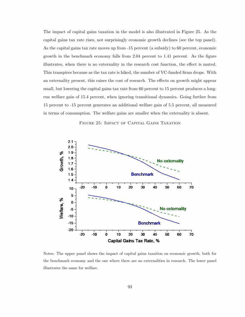
The impact of capital gains taxation in the model is also illustrated in Figure 25. As the
capital gains tax rate rises, not surprisingly economic growth declines (see the top panel).
As the capital gains tax rate moves up from -15 percent (a subsidy) to 60 percent, economic
growth in the benchmark economy falls from 2.04 percent to 1.41 percent. As the figure
illustrates, when there is no externality in the research cost function, the effect is muted.
This transpires because as the tax rate is hiked, the number of VC-funded firms drops. With
an externality present, this raises the cost of research. The effects on growth might appear
small, but lowering the capital gains tax rate from 60 percent to 15 percent produces a long-
run welfare gain of 15.4 percent, when ignoring transitional dynamics. Going further from
15 percent to -15 percent generates an additional welfare gain of 5.5 percent, all measured
in terms of consumption. The welfare gains are smaller when the externality is absent.
Figure 25: Impact of Capital Gains Taxation
Notes: The upper panel shows the impact of capital gains taxation on economic growth, both for
the benchmark economy and the one where there are no externalities in research. The lower panel
illustrates the same for welfare.
93

2.13. What about Growth?
Is the recent rise in VC investment reflected in growth statistics? The answer to this question
is nuanced. On the one hand, at the country level VC investment appears to be positively
linked with economic growth. A scatter plot between economic growth and VC investment
for G7 countries is shown in the upper panel of Figure 26. These are developed nations.
As the figure shows, there is a clear positive association between these two variables. The
analysis is extended to G20 countries in the bottom panel of the figure. Now the scatter
plot includes some poorer countries, where VC investment isn’t so prevalent. There is still
a positive association, but not surprisingly it is weaker.
To conduct a more formal analysis, some regression analysis is conducted with a sample
of 37 economies over the period 1995 to 2014. The sample covers 99 percent of world VC
investment and 88 percent of world GDP. In addition, the two-decade sampling period is
divided into four sub-periods, each lasting five years. A country is included in the sample
if its share of world VC investment between 1995 and 2014 is not less than 0.05 percent.10
The dependent variable in the regression analysis is the median growth rate of real GDP
per capita in each period, while the main explanatory variable is the natural logarithm
of the median VC investment-to-GDP ratio. The regressions include the initial levels of
real GDP per capita and the Barro and Lee (2013) human capital index. These control
variables are the two main factors demonstrated in the empirical literature to be important
for economic growth. Moreover, period dummies are included to control for aggregate
shocks to all countries. An IV approach is also taken to address the endogeneity issues.
Two IVs are used. The first, which follows the strategy pioneered in Barro and Lee (1994),
is the median VC investment-to-GDP ratio for each country during the decade preceding
the sample period (i.e., 1985 to 1994). The second is a dummy variable for the legal origin
of the country, which is equal to 1 for common-law countries. The idea is that common-law
legal systems foster better financial development than civil-law legal systems, because of
higher judicial independence from the government and the flexibility of the courts to adapt
10An exception is Bermuda, which accounted for 0.18 percent of world VC investment. Bermuda isexcluded because it is a tax haven. Companies set up offices there, while undertaking virtually no businessactivity, just to avoid corporate income taxation.
94

to changing conditions (see Beck, Demirguc-Kunt, and Levine (2005)).
Figure 26: Economic Growth and VC Investment, 1995-2014
Notes: The upper panel shows the relationship between VC investment and growth in G7 countries,
while the bottom panel does the same for the G20.
The main regression results are reported in Table 16. As the table shows, VC and growth
are positively correlated. The IV estimate for the G7 countries in the last regression in
Panel A shows that a 10 percent increase in the VC investment-to-GDP ratio is connected
with a 0.024 percentage point increase in growth. This may seem small, but it implies that
increasing the VC investment-to-GDP ratio from the Japanese level (0.003 percent) to the
U.S. level (0.19 percent) would increase growth by 1.01 percentage points.11
11Relatedly, Sampsa and Sorenson (2011) estimate, using a panel of U.S. metropolitan statistical areas,that VC positively affects startups, employment, and regional income.
95

Table 16: VC Investment and Growth: Cross-Country Regressions
Dependent variable Growth of GDP
OLS IV
Pre ln(VC Inv/GDP) Legal origin Both
Panel A: G7
ln(VC Inv/GDP) 0.186** 0.253*** 0.227** 0.240***
(0.0782) (0.0910) (0.0899) (0.0816)
Observations 28 28 28 28
R-squared 0.695
Panel B: 37-Country Sample
0.228** 1.156** 0.421* 0.463*
(0.112) (0.501) (0.254) (0.260)
Observations 148 120 148 120
R-squared 0.295
Notes: See the main text for a description of the dependent and independent variables. Pre ln(VC
Inv/GDP) refers to the pre-sample VC investment-to-GDP ratio. Standard errors are in parentheses.
***, **, and * denote significance at the 1, 5 and 10 percent levels.
On the other hand, the impact of VC may not be readily apparent in growth statistics for
several reasons. First, technological revolutions, such as the Information Age, may cause
disruptions in an economy. Old forms of businesses are displaced by new forms. Online re-
tailing is displacing brick and mortar stores, for example. Greenwood and Yorukoglu (1997)
discuss how the dawning of the First and Second Industrial Revolutions were associated with
productivity slowdowns and suggest that the same phenomena characterize the Information
Age. Second, measuring investment and output in the information age is difficult. Think
about the introduction of cell phones, as discussed in Hulten and Nakumura (2017). Cell
phones substitute for traditional land lines, audio players, cameras, computers, navigation
systems, and watches, inter alia. Cell phones have free apps. Between 1988 and 2015, land
lines fell from 1.7 to 0.3 percent of personal consumption expenditures. Since cell phones
constitute 0.15 percent of personal consumption expenditures, this would be measured as a
96

drop or slowdown in GDP. An iPhone 5 would have cost more than $3.56 million to build
in 1991.12 Likewise, global camera production dropped from 120 million units to 40 mil-
lion over the 2007 to 2014 period. Additionally, investment may be in intangibles, such as
software, R&D, retraining workers, reconfiguring products and organizational forms, and
branding new products. Corrado, Hulten, and Sichel (2009) estimate that investment in
such intangibles is now as large as that in tangibles. Including intangible investment in
GDP accounting could increase estimates of growth by 10 to 20 percent. McGrattan and
Prescott (2005) argue that, after taking intangibles into account, the 1990s was a boom
period. Third, technologies flow across national boundaries. So even countries that don’t
innovate will experience growth from the adoption of new technologies. Out of France, Ger-
many, Japan, the United Kingdom, and the United States, Eaton and Kortum (1999) find
that only the United States derived most of its growth from domestic innovation. Comin
and Hobijn (2010) document that diffusion lags for new technologies have shrunk over time.
Fourth, firms may park the profits from new innovation offshore to avoid taxation. Account-
ing for this could increase productivity growth by 0.25 percentage points over the 2004 to
2008 period, according to Guvenen et al. (2017).
2.14. Conclusion
Venture capital is important for economic growth. Funding by venture capitalists is pos-
itively associated with patenting activity. VC-backed firms have higher IPO values when
they are floated. Following flotation they have higher R&D-to-sales ratios. VC-backed firms
also grow faster in terms of employment and sales.
An endogenous growth model of the VC process is constructed and taken to the data. In the
framework, entrepreneurs bring ideas to venture capitalists for funding. Venture capitalists
provide seed money to research the ideas. After this projects enter a funding-round cycle.
During each round, projects are: (i) evaluated to assess their ongoing viability; (ii) those
that pass are then provided with VC to develop the project; (iii) the use of funds is monitored
12This 2017 guesstimate was done by Bret Swanson, who calculates that the flash memory, processor,and broadband communications of an iPhone 5 would have cost $1.44, $0.62, and $1.5 million in 1991. Thecost of these three components adds up to $3.56 million. On top of that, considering the other components(camera, iOS operating system, motion detectors, display, apps, etc), it would have cost more than $3.56million to build an iPhone 5 in 1991.
97

is done to ensure that there is no malfeasance; and (iv) successful projects are floated on
the stock market or sold to other businesses. The evaluation plan, development funding,
the monitoring strategy, and the equity share of the venture capitalist are governed by a
dynamic contract between the entrepreneur and a venture capitalist. The model is capable of
matching several stylized facts of the VC process by funding round. In particular, it mimics
the funding-round profiles for the success and failure rates of projects, the injections of VC
for development, the venture capitalist’s share of equity, and the value of an IPO by the
time it takes to go to market. This is done while matching the share of VC-backed firms
in total employment and the average size of a VC-backed firm relative to a non-VC-backed
one.
The key personnel involved with starting up the enterprises funded by venture capitalists
are rewarded in the form of convertible equity and stock options. In the United States,
venture capitalists are subject only to capital gains taxation. The rate at which VC-funded
startups are taxed in the United States is low relative to other developed countries. Does
this promote innovative activity? The analysis suggests that raising the tax on VC-funded
startups from the U.S. rate of 15 percent to the Portugese rate of nearly 60 percent would
shave 0.4 percentage points off growth and lead to a long-run consumption-equivalent welfare
loss of 15.4 percent.
98

APPENDIX
A.1. Appendix for Chapter 1
Data Sources
Detailed information of the patents granted in the United States Patent and Trademark
Office (USPTO) between 1976 and 2006 is offered in the NBER-USPTO Utility Patents
Grant Data (PDP).1 Accounting information of the publicly held corporations is available
in Compustat North American Fundamentals (Annual) retrieved from Wharton Research
Data Services. The matching between patent assignees and corporate entities are developed
in the NBER Patent Data Project.
Litigation information of a patent is obtained by combining three data sets: Lex Machina
Database on Patent Litigations, Derwent Litalert Database on Patent Litigations, and
UGA Patent Litigation Datafile. For patents involved in litigation after 2000, Lex Machina
Database on Patent Litigations is the most thorough data base.2 Information on litigated
patents before 2000 relies on Derwent Litalert Database on Patent Litigations.3 However,
neither Lex Machina Database nor Derwent Litalert Database provides information on the
detailed court decisions. To address this issue, UGA Patent Litigation Datafile is applied.
This dataset covers all patent-related cases where at least one court decision (district or
appellate court) is recorded in the United States Patents Quarterly (USPQ). USPQ main-
tained the same publisher since 1929, and it includes the entire opinions for all appellate
court decisions and a large sample of district court decisions (especially when they constitute
important precedents for later judicial review)4.
In the cross-country study, the national account information of countries is based on the
1Source link to NBER-USPTO Utility Patents: https://sites.google.com/site/patentdataproject/Home2Source link: https://lexmachina.com/3More detailed information can be found in Galasso, Schankerman, and Serrano (2013).4Source link of UGA Patent Litigation Datafile: http://people.terry.uga.edu/jlturner/patentlitigationdata/
99

World Development Indicator of the World Bank.5 The Barro and Lee (2013) human capital
index is contained in the Penn World Table.6 The import and export of each country with
the U.S. is gathered from Schott (2008).7
A.2. Appendix for Chapter 2
A.2.1. Data Appendix
Figures
• Figure 15: The rise of venture capital, 1970 to 2015. Investment by venture capitalists
is obtained from the VentureXpert database of Thomson ONE. The fraction of public
firms backed by VC companies is created by matching firm names in VentureXpert
and CompuStat; the latter are available from Wharton Research Data Services.8
• Figure 16: The share of VC-backed companies in employment, R&D spending, and
patents. The employment and R&D shares of VC-backed public companies are cal-
culated by matching firm names in VentureXpert and CompuStat, as in Figure 15.
The share of patents for VC-backed public companies is computed by matching firm
names in VentureXpert and the NBER Patent Data Project.9
• Figure 19: Investment and equity share by funding round. Investment in each fund-
ing round is based on the VC-funded deals in Crunchbase between 1981 and 2015.
Crunchbase has better funding-round information than VentureXpert. The vertical
axis is the mean of funding in a round across all deals, from round 1 (i.e., series A)
to round 7 (i.e., series G). Funding is converted into millions of constant $2009 using
the GDP deflator. The mean duration of a funding round in Crunchbase is 1.4 years,
which is taken to 1.5 years here. The share of equity transferred to the venture capi-
5Source link to the World Development Indicator: https://data.worldbank.org/data-catalog/world-development-indicators.
6Source link of Penn World Table (Version 8.0): http://cid.econ.ucdavis.edu/pwt.html7Source link: http://faculty.som.yale.edu/peterschott/sub international.htm8Source link: https://wrds-web.wharton.upenn.edu/wrds/index.cfm?9Source link: https://sites.google.com/site/patentdataproject/Home
100

talist in each funding round is calculated as the ratio of VC funding in each round to
the post-money valuation of the company after the VC investment. For each funding
round the mean equity share across all deals is calculated. The vertical axis is the
cumulated share of equity transferred to the venture capitalist.
• Figure 20: The odds of success and failure by funding round and the value of an
IPO by the duration of funding. The underlying data source is Puri and Zarutskie
(2012, Table VI.B, p. 2271). The success rate refers to firms that have an IPO or
that are acquired by another firm. The acquisitions in Puri and Zarutskie (2012)
are converted into successes by multiplying by 0.629. This is based on the fact that
the cash multiple for acquisitions is 37.1 percent lower than for IPOs, as reported in
Achleitner et al. (2012). In addition, the success and failure rates by funding round
are obtained by interpolating the original annual data using a cubic spline to get a
periodicity of 1.5 years. Puri and Zarutskie (2012, Table V) classify a firm “as having
failed if it disappears from the LBD in its entirety.” The value of an IPO, as a function
of the duration of VC funding, derives from regression (2) in Table 17 (discussed in
Section A.2.1).
• Figure 24: The cross-country relationship between the tax rate on VC activity and the
VC investment-to-GDP ratio. The source for the cross-country data is Henrekson and
Sanandaji (2016, Table 1) .
• Figure 26: Economic growth and VC investment. VC investment and the growth rate
of real GDP per capita are based on VentureXpert of Thomson ONE and the World
Development Indicators of the World Bank, respectively.
Tables
• Table 8: Top 30 VC-Backed Companies. As in Figure 15, the list of VC-backed public
companies is gathered by matching firm names in VentureXpert and CompuStat.
101

• Table 9: VC versus Non-VC-Backed Public Companies. The VC-backed public com-
panies are singled out by matching firm names in VentureXpert and CompuStat. Since
the R&D-to-sales ratio and growth rates can be very volatile across firms, the top and
bottom 5 percent of the outliers are trimmed in this regression. The results are robust
to changing the trimming threshold (at the 1 percent versus 5 percent level).
• Table 10: VC and Patenting, Firm-Level Regressions. The VC-funded patentees are
identified by matching firm names in VentureXpert and PatentsView.10 The capi-
tal gain taxes are accessed from TAXSIM, an NBER tax simulation program.11 In
calculating the dependence on external finance, 30 percent of selling, general, and ad-
ministrative expenses is taken as intangible investment. The industry-level of private
and federally funded R&D is collected from the Business R&D and Innovation Survey
by the National Science Foundation.12 A truncation adjustment for citations is made
following Bernstein (2015). The industry dummies in this regression are at the 2-digit
SIC level.
• Table 11: VC and Patenting, Industry-Level Regressions. The product of the dereg-
ulation dummy and dependence on external finance is used as the IV for the cross
term between VC funding and dependence on external finance. The industry panel is
based on the 4-digit SIC. The industry dummies in this regression are at 2-digit SIC
level.
• Table 16: VC Investment and Growth, Cross-Country Regressions. The full sample
covers 37 economies between 1995 and 2014. As in Figure 26, VC investment is from
VentureXpert and the GDP growth rate is from the World Development Indicators.
The Barro and Lee (2013) human capital index is a measure of educational attainment
at the country level. The IVs are the median VC investment-to-GDP ratio (in natural
logarithm) for each country between 1985 and 1994, and a dummy variable for legal
10Source link of PatentsView: http://www.patentsview.org/download/.11Source link of TAXSIM: http://users.nber.org/˜taxsim/state-rates/.12Source link of BRDIS: https://www.nsf.gov/statistics/srvyindustry/#tabs-2.
102

origin (equal to 1 for common-law countries) a la Beck, Demirguc-Kunt, and Levine
(2005).
Duration of VC Funding and the Value of an IPO
The relationship between the firm’s value at an IPO and the number of years it received
funding from the venture capitalist is examined using regression analysis. The regressions
are based on public companies funded by venture capitalists between 1970 and 2015. These
VC-backed companies are identified by matching firm names in CompuStat and VentureX-
pert. The dependent variable in the regressions is the natural logarithm of the market value
of the firms at IPO (in $2009). A three-year average is used for market value because of
the notorious volatility of share prices following an IPO. IPOs are excluded when they take
more than 11 years for the firms to go public after receiving the first VC funding. This is for
two reasons: (i) the sampling period is formulated to be consistent with the model where
the maximum duration for each VC investment is 10.5 years, and (ii) only 4.5 percent of
the observations occur after 11 years with the data being very noisy. The main explanatory
variable is the number of years between the firm’s first VC funding and the date of its IPO.
The findings are shown in Table 17. The first coefficient in regression (2) is used in Figure
20 to plot the decline in the value of an IPO across successive funding rounds.
103

Table 17: VC Funding and Years to Go Public
Dependent variable ln(Firm value at IPO, real)
1 2
years btw first VC funding and IPO -0.0470*** -0.0385***
(0.0161) (0.0146)
firm age at IPO -0.0246***
(0.00495)
# of employees at IPO (log) 0.709***
(0.0375)
year dummy for IPO N Y
industry effect N Y
Observations 1,042 1,006
R-squared 0.008 0.627
Notes: Standard errors are in parentheses. ***, **, and * denote significance at the 1, 5 and 10
percent levels.
A.2.2. Theory Appendix
Proofs for Lemmas 2 and 4 are supplied in turn here. Lemma 2 establishes the existence of
a balanced-growth path. Lemma 4 shows that solving the contract problem (P2) subject
to a sequence of one-shot incentive constraints is equivalent to solving it subject to a single
consolidated round-0 incentive constraint that allows for multi-shot deviations. This is
proved using Lemma 3 as an intermediate step.
Balanced Growth
Lemma 2 (Balanced Growth) There exists a balanced-growth path of the form outlined in
Section 2.9.
104

Proof. Suppose that pt, σt, µt, βt solves the old problem for x and x. It will be shown
that gwpt, σt, µt, βt solves the new one for x′ = gxx and x′ = gxx. First, observe
that if x′ = gxx and x′ = gxx, then I(x′; gtxx′) = gwI(x; gtxx). This occurs because
T (x′; x′t) = gwT (x; xt). This can be seen from (P1) because x will rise by gx and wages by
gw. If p′t = gwpt, then it is immediate from the objective function in (P2) that C(x′; x′) =
gwC(x; x). Now, consider the incentive constraint (2.5). At the conjectured solution, the
left-hand side will inflate by the factor gw. So will the right-hand side because D(σ′t) −
D(σ′t) = gw[D(σt)−D(σt)], since all costs are specified as a function of w. Therefore, the
new solution still satisfies the incentive constraint. Move now to the zero-profit constraint
(2.6). Again, the left-hand side will inflate by the factor gw, since p′t = gwpt, φ
′t = gwφt,
D(σ′t) = gwD(σt), Mt(µ′t) = gwMt(µt), E(β
′t) = gwE(βt), and R(x′/x′, e) = gwR(x/x, e).
This is trivially true for the right-hand side. Hence, the zero-profit constraint holds at the
new allocations. It is easy to deduce from the right-hand side of (2.5) that the old solution
for σt will still hold. This can be seen by using the above argument while noting that
D1(σ′t) = gwD1(σt). To sum up, at the conjectured new solution, the objective function
and the constraints all scale up by the same factor of proportionality gw. By cancelling out
this factor of proportionality, the new problem reverts back to the old one. Likewise, it is
easy to deduce that if x solves problem (P3) for x, then x′ = gxx solves it when x′ = gxx.
The occurs because problem (P3) also scales up by the factor of proportionality gw. When
x/x remains constant along a balanced-growth path, then the initial research cost of the
project will rise at the same rate as wages, gw. Additionally, V (x) will grow the same rate
as wages, w, so from (2.7) it is apparent that e will remain constant.
One-Shot Deviations versus Multi-Shot Deviations
This is an intermediate step toward solving Lemma 4. To this end, it will be shown that
if the incentive constraint (2.5) holds for round t, when the entrepreneur has not deviated
up to and including round t− 1, then it will also hold when he follows some arbitrary path
of deviations up to and including round t− 1. Let αt represent that the probability that a
105

project is good at round t as defined by (2.4). These odds evolve recursively according to
αt+1 =(1− σt)αt
(1− σt)αt + (1− βt+1)(1− αt),
where α1 = ρ/[ρ+(1−ρ)(1−β1)]. For use in proving Lemma 3, note that αt+1 is increasing
in αt and decreasing in σt. This implies that if the entrepreneur deviates in round t, so that
σt < σt, he will be more optimistic about the future, as αt+1 will be higher. This increases
the value of the α’s for future rounds as well. With this notation, the round-t incentive
constraint (2.5) then reads
αt(1− τ)δσt[I(x; gtxx)− pt] + (1− σt)T∑
i=t+1
Πi−1j=t+1(1− σj)δ
i+1−tσi[I(x; gixx)− pi]
≥ (1− µt)maxσt
(D(σt)−D(σt)
+αt(1− τ)δσt[I(x; gtxx)− pt] + (1− σt)T∑
i=t+1
Πi−1j=t+1(1− σj)δ
i+1−tσi[I(x; gixx)− pi]).
Lemma 3 If the incentive constraint (2.5) holds for round t, when the entrepreneur has
not deviated up to and including in round t− 1, then it will also hold when he follows some
arbitrary path of deviations up to and including in round t− 1.
Proof. Suppose that the entrepreneur deviates in some manner before round t. Let αt be
the prior associated with this path of deviation. Since the σ’s will be less that than the σ’s,
it follows that αt > αt. Let σt be the optimal round-t deviation associated with αt. Now,
αt(1− τ)δσt[I(x; gtxx)− pt] + (1− σt)T∑
i=t+1
Πi−1j=t+1(1− σj)δ
i+1−tσi[I(x; gixx)− pi]
≥ (1− µt)(D(σt)−D(σ)
+αt(1− τ)δσt[I(x; gtxx)− pt] + (1− σt)T∑
i=t+1
Πi−1j=t+1(1− σj)δ
i+1−tσi[I(x; gixx)− pi]),
106

because σt is maximal when the prior is αt, while σt is not. Next, replace αt with αt to get
αtδσt[I(x; gtxx)− pt] + (1− σt)T∑
i=t+1
Πi−1j=t+1(1− σj)δ
i+1−tσi[I(x; gixx)− pi]
≥ (1− µt)(D(σt)−D(σt)
+ αtδσ[I(x; gtxx)− pt] + (1− σt)T∑
i=t+1
Πi−1j=t+1(1− σj)δ
i+1−tσi[I(x; gixx)− pi]),
since αt > αt. Last, if the prior is αt, then σt is maximal, so the above equation can be
rewritten as
αt(1− τ)δσt[I(x; gtxx)− pt] + (1− σt)T∑
i=t+1
Πi−1j=t+1(1− σj)δ
i+1−tσi[I(x; gixx)− pi]
≥ (1− µt) maxσt
(D(σt)−D(σt)
+ αt(1− τ)δσt[I(x; gtxx)− pt] + (1− σt)T∑
i=t+1
Πi−1j=t+1(1− σj)δ
i+1−tσi[I(x; gixx)− pi]).
The Consolidated Round-0 Incentive Constraint
The consolidated round-0 incentive constraint is
(1− τ)∑T
t=1 ρΠt−1j=1(1− σj)δ
tσt[I(x; gtxx)− pt] ≥
maxσtTt=1∑T
t=1 δt−1[ρΠt−1
j=1(1− σj) + (1− ρ)Πtj=1(1− βj)]
×(1− µt)[D(σt)−D(σt)]
+(1− τ)∑T
t=1 ρΠt−1j=1(1− σj)δ
tσt[I(x; gtxx)− pt].
(A.1)
Lemma 4 (Equivalence of contracts) A contract βt, σt, µt, pt solves problem (P2) subject
107

to the sequence of one-shot incentive constraints (2.5) if and only if it solves (P2) subject
to the consolidated time-0 incentive constraint (A.1).
Proof. (Necessity) Suppose that an allocation satisfies the one-shot incentive compatibility
constraints (2.5) but that it violates the consolidated one (A.1). This implies that at some
round in the problem with the consolidated constraint it pays to deviate and pick a σt 6=
σt. Pick the last round of deviation (which may be T ). It must be true that σt solves the
maximization problem
(1− µt) maxσt
(D(σt)−D(σt)
+ αt(1− τ)δσ[I(x; gtxx)− pt] + (1− σt)T∑
i=t+1
Πi−1j=t+1(1− σj)δ
i+1−tσi[I(x; gixx)− pi]),
where αt is the prior associated with the path of σ’s up to round t− 1, which may include
previous deviations. But, as was shown in Lemma 3, this is less than the value of sticking
with the contract or
αt(1− τ)δσt[I(x; gtxx)− pt] + (1− σt)T∑
i=t+1
Πi−1j=t+1(1− σj)δ
i+1−tσi[I(x; gixx)− pi],
when the round-t one-shot incentive constraint (2.5) holds, as assumed.
(Sufficiency) Suppose σtTt=1 satisfies the consolidated incentive constraint, but violates
108

the one-shot incentive constraint at round k. Then, using (2.4) and (2.5), it follows that
ρΠk−1j=1(1− σj)δk−1(1− τ)δσk[I(x; gkxx)− pk]
+(1− σk)T∑
t=k+1
Πt−1j=k+1(1− σj)δ
t+1−kσt[I(x; gtxx)− pt]
= (1− τ)∑T
t=k ρΠt−1j=1(1− σj)δ
tσt[I(x; gtxx)− pt]
< δk−1(1− µk)(
[ρΠk−1j=1(1− σj) + (1− ρ)Πk
j=1(1− βj)][D(σk)−D(σk)]
+ρΠk−1j=1(1− σj)(1− τ)δσk[I(x; gkxx)− pk]
+(1− σk)T∑
t=k+1
Πt−1j=k+1(1− σj)δ
t+1−kσt[I(x; gtxx)− pt]).
(A.2)
The left-hand side gives the payoff in the contract at the optimal solution from round k on,
when using the consolidated incentive constraint, while the right-hand side represents the
payoff from a one-shot deviation at round k. Now the objective function for the contract
can be written as
(1− τ)k−1∑t=1
ρΠt−1j=1(1− σj)δ
tσt[I(x; gtxx)− pt] + (1− τ)T∑t=k
ρΠt−1j=1(1− σj)δ
tσt[I(x; gtxx)− pt].
Evaluate this at the optimal solution for the contract when using (A.1) instead of (2.5).
Next, in this objective function, replace the payoff from round k on, as represented by
the left-hand side of (A.2), with the payoff from the one-shot deviation as given by the
right-hand side. This deviation would increase the value of the objective function for the
entrepreneur, which is a contradiction.
109

BIBLIOGRAPHY
Acemoglu, D. and U. Akcigit. (2012). “Intellectual Property Rights Policy, Competitionand Innovation.” Journal of the European Economic Association, 10, 1-42.Achleitner, Ann-Kristin, Braun, Reiner, Lutz, Eva and Uwe Reiner. 2012. “VentureCapital Firm Returns from Acquisition Exits.” Unpublished paper, Technische UniversitatMunchen.Aghion, Philippe and Peter Howitt (1992). “A Model of Growth Through Creative De-struction”, Econometrica, 110, 323 – 351.Akcigit U., Celik M., Greenwood J., 2016. “Buy, Keep or Sell: Economic Growth and theMarket for Ideas.” Econometrica, Econometric Society, vol. 84, pages 943 – 984, 05.Arrow, Kenneth (1962). “Economic Welfare and the Allocation of Resources for Invention”,in R.R. Nelson, ed. Universities-National Bureau of Economic Research Conference Series;The Rate and Direction of Economic Activities: Economic and Social Factors, PrincetonUniversity Press, New York.Anderson, E., Schmittlein, D., 1984. “Integration of the sales force: an empirical examina-tion.” RAND Journal of Economics, 15, 385 – 395.John R. Allison, Mark A. Lemley, David L. Schwartz, 2014. “Understanding the Realitiesof Modern Patent Litigation.” Texas Law Review, 1769.Atkinson S., Marco A., and Turner J. 2009. “The Economics of a Centralized Judiciary:Uniformity, Forum Shopping and the Federal Circuit”, Journal of Law and Economics, 52,pages 411 – 43.Barro, Robert J. and Jong-Wha Lee. 1994. “Sources of Economic Growth.” Carnegie-Rochester Conference Series on Public Policy, 40: 1-46.Barro, Robert J. and Jong-Wha Lee. 2013. “A New Data Set of Educational Attainmentin the World, 1950–2010.” Journal of Development Economics, 104 (C): 184-198.Beck, Thorsten, Demirguc-Kunt, Asli, and Ross Levine. 2005. “Law and Firms’ Access toFinance.” American Law and Economics Review, 7 (1): 211-252.Bergemann, Dirk and Ulrich Hege. 1998. “Venture capital financing, moral hazard, andlearning.” Journal of Banking and Finance, 22 (6): 703-735.Bernstein, Shai, Giroud, Xavier and Richard R. Townsend. 2016. “The Impact of VentureCapital Monitoring.” Journal of Finance, 71 (4): 1591–1622.Clementi, Gian Luca and Hugo Hopenhayn. 2006. “A Theory of Financing Constraintsand Firm Dynamics.” Quarterly Journal of Economics, 121 (1): 229-265.Coase, Ronald H., 1937. “The Nature of the Firm.” Economica, 4 (16), 386 – 405.Cole, Harold L., Greenwood, Jeremy and Juan M. Sanchez. 2016. “Why Doesn’t Technol-ogy Flow from Rich to Poor Countries?” Econometrica, 84 (4): 1477-1521.Comin, Diego and Bart Hobijn. 2010. “An Exploration of Technology Diffusion.” AmericanEconomic Review, 100 (5): 2031–2059.Cooley, T.F., and E.C. Prescott, 1995.“Economic Growth and Business Cycles”, Frontiersof Business Cycle Research, ed. by T.F. Cooley. Princeton, NJ: Princeton University Press,1 – 38.Corrado C., C. Hulten, and D. Sichel, 2009. “Intangible Capital and U.S. EconomicGrowth”, Review of Income and Wealth, 55, 661 – 685.Eaton, Jonathon and Samuel Kortum. 1999. “International Technology Diffusion: Theory
110

and Measurement.” International Economic Review, 40 (3): 537-570.Gilbert, Richard. and Carl Shapiro (1990). “Optimal Patent Length and Breadth”, Journalof Industrial Economics, 21(1), 106 – 112.Gompers, Paul, Gronell, Will, Kaplan, Steven N, and Ilya A. Strebulaev. 2016. “How DoVenture Capitalists Make Decisions?” Unpublished paper.Gompers, Paul and Josh Lerner. 2006. The Venture Capital Cycle. Cambridge, MA: TheMIT Press.Greenwood, Jeremy and Mehmet Yorukoglu. 1997. “1974.” Carnegie-Rochester ConferenceSeries on Public Policy, 46: 49-95.Grossman, Sanford J., and Oliver Hart. 1986. “The Costs and Benefits of Ownership: ATheory of Vertical and Lateral Integration.” Journal of Political Economy, 94(4): 691 –719.Grossman, Gene and Elhanan Helpman (1990). Innovation and Growth in the Global Econ-omy, Cambridge, MA, MIT Press.Guner, Nezih, Ventura, Gustavo, and Daniel Yi Xu. 2008. “Macroeconomic Implicationsof Size-Dependent Policies.” Review of Economic Dynamics, 11: 721-744.Guvenen, Fatih, Mataloni Jr., Raymond J., Rassier, Dylan G., and Kim J. Ruhl. 2017.“Offshore Profit Shifting and Domestic Productivity Measurement.” Unpublished paper,University of Minnesota.Hall, B.H., A.B. Jaffe, and M. Trajtenberg, 2001. “The NBER Patent Citations Data File:Lessons, Insights and Methodological Tools.” Working Paper 8498, NBER.Hart, Oliver, and John Moore. 1990. “Property Rights and the Nature of the Firm.” Jour-nal of Political Economy, 98(6): 1119 – 58.Hart, Oliver. 1995. “Firms, Contracts, and Financial Structure.” Clarendon Lectures inEconomics. Oxford and New York: Oxford University Press, Clarendon Press.Hart, Oliver, and Jean Tirole. 1990. “Vertical Integration and Market Foreclosure.” Brook-ings Papers on Economic Activity: Microeconomics, 205 – 76.Henrekson, Magnus and Tino Sanandaji. 2016. “Stock Option Taxation and Venture Cap-ital Activity: A Cross-Country Study.” IFN Working Paper No. 1104, Research Instituteof Industrial Economics.Henry, Matthew D.; McGahee, Thomas P.; Turner, John L. 2013. “Dynamics of PatentPrecedent and Enforcement: An Introduction to the UGA Patent Litigation Datafile.” Uni-versity of Georgia Working Paper.Hopenhayn H., Llobet G., Mitchell M., 2006. “Rewarding Sequential Innovators: Prizes,Patents, and Buyouts.” Journal of Political Economy, University of Chicago Press, vol.114(6), pages 1041 – 1068.Hopenhayn H., Mitchell M., 2001. “Innovation Variety and Patent Breadth.” RAND Jour-nal of Economics, The RAND Corporation, vol. 32(1), pages 152 – 66.Hulten, Charles and Leonard Nakamura. 2017. “We See the Digital Revolution EverywhereBut in GDP.” Presentation, Office for National Statistics, UK.Lerner, Josh, 1995. “Patenting in the Shadow of Competitors,” Journal of Law and Eco-nomics, University of Chicago Press, vol. 38(2), pages 463–495.Joskow, P., 1985. “Vertical integration and long-term contracts: the case of coal-burningelectric generation plants.” Journal of Law, Economics, and Organization 1, 33 – 80.Jovanovic, Boyan and Balazs Szentes. 2013. “On the Market for Venture Capital.” Journal
111

of Political Economy, 121 (3): 493-527.Karaivanov, Alexander and Robert M. Townsend. 2014. “Dynamic Financial Constraints:Distinguishing Mechanism Design From Exogenously Incomplete Regimes.” Econometrica,82 (3): 887–959.Kenney, Martin. 2011. “How Venture Capital Became a Component of the US NationalSystem of Innovation.” Industrial and Corporate Change, 20 (6): 1677–1723.Kerr, William R. 2010. “Breakthrough Inventions and Migrating Clusters of Innovation.”Journal of Urban Economics, 67 (1): 46–60.Khan, Hashmat and Pythagoras Petratos. 2016. “Entrepreneurship and the Business Cy-cle: Stylized Facts from U.S. Venture Capital Activity.” CEP 16-09, Carleton University.Klein, B., 1988. “Vertical integration as organizational ownership: the Fisher Body-GeneralMotors relationship revisited”. Journal of Law, Economics, and Organization, 4, 199 – 213.Klein, B., 2000b. “Fisher-General Motors and the nature of the firm”. Journal of Law andEconomics, 43, 105 – 141.Klemperer, Paul (1990). “How Broad Should the Scope of Patent Protection Be?”. Journalof Industrial Economics, 21, 113 – 130.Kortum, Samuel and Josh Lerner. 2000. “Assessing the Contribution of Venture Capitalto Innovation.” Rand Journal of Economics, 31 (4): 674-692.Lamoreaux, Naomi, Levenstein, Margaret, and Kenneth L. Sokoloff. 2007. “Financing In-vention during the Second Industrial Revolution: Cleveland, Ohio, 1870-1920.” In NaomiLamoreaux and Kenneth L. Sokoloff, eds., Financing Innovation in the United States, 1870to the Present. Cambridge: The MIT Press, 39-84.Levine, Ross. 2005. “Finance and Growth: Theory and Evidence.” In Philippe Aghion andSteven N. Durlauf, eds., Handbook of Economic Growth, Vol. 1A, Amsterdam: Elsevier,865-934.Mansfield, Edwin, Schwartz, Mark and Wagner, Samuel, 1981. “Imitation Costs andPatents: An Empirical Study”, Economic Journal, 91, issue 364, page 907 – 18.Masten, S., 1984. “The organization of production: evidence from the Aerospace industry”.Journal of Law and Economics, 27, 403 – 417.McGrattan, Ellen R. and Edward C. Prescott. 2005. “Productivity and the Post-1990 U.S.Economy.” Federal Reserve Bank of St. Louis Review, 87 (4): 537-49.Megginson, William L. and Kathleen A. Weiss. 1991. “Venture Capitalist Certification inInitial Public Offerings.” Journal of Finance, 46 (3) (Papers and Proceedings): 879-903.Monteverde, K., Teece, D., 1982. “Supplier switching costs and vertical integration in theautomobile industry”, Bell Journal of Economics, 13, 206 – 212.Opp, Christian. 2018. “Venture Capital and the Macroeconomy.” Unpublished paper, Uni-versity of Pennsylvania.Parente, Stephen L. 1993. “Technology Adoption, Learning-by-Doing, and Economic Growth.”Journal of Economic Theory, 63 (2): 346-369.Park, Walter G., 2008. “International patent protection: 1960-2005.” Research Policy, El-sevier, vol. 37(4), pages 761 – 766.Phelan, Christopher and Robert M. Townsend. 1991. “Computing Multi-Period, Information-Constrained Optima.” Review of Economic Studies, 58 (5): 853-881.Puri, Manju and Rebecca Zarutskie. 2012. “On the Life Cycle Dynamics of Venture-Capitaland Non-Venture-Capital-Financed Firms.” Journal of Finance, LXVII (6): 2247-2293.
112

Rajan, Raghuram G. and Luigi Zingales. 1998. “Financial Dependence and Growth.”American Economic Review, 88 (3): 559-586.Romer, Paul M. 1986. “Increasing Returns and Long-Run Growth.” Journal of PoliticalEconomy, 94 (5): 1002–1037.Romer, Paul M. (1990). “Endogenous Technological Change”, Journal of Political Econ-omy, 98, S71 – S102.Samila, Sampsa and Olav Sorenson. 2011. “Venture Capital, Entrepreneurship, and Eco-nomic Growth.” Review of Economics and Statistics, 93 (1): 338–349.Schott, Peter K. “The relative sophistication of Chinese exports,” Economic Policy, vol.23, pages 5 – 49, 01.Scotchmer, Suzanne (1999). “On the Optimality of the Patent System.” The Rand Journalof Economics, 30, 181 – 196. Silveira, Rafael and Randall D. Wright. 2016. “VentureCapital: A Model of Search and Bargaining.” Review of Economic Dynamics, 19: 232–246.Tirole, Jean (1988). The Theory of Industrial Organization, MIT Press, Cambridge, Mas-sachusetts.Townsend, Robert M. 1979. “Optimal Contracts and Competitive Markets with CostlyState Verification.” Journal of Economic Theory, 21 (2): 256-293.Williamson, Oliver E, 1971. “The Vertical Integration of Production: Market Failure Con-siderations.” American Economic Review, 61 (2): 112 – 23.Williamson, Oliver E. 1979. “Transaction-Cost Economics: The Governance of Contrac-tural Relations.” Journal of Law and Economics, 22 (2): 233 – 61.Williamson, Oliver E. 1983. “Credible Commitments: Using Hostages to Support Ex-change.” American Economic Review, 73(4): 519 – 40.Williamson, Stephen D. 1986. “Costly Monitoring, Financial Intermediation, and Equilib-rium Credit Rationing.”Journal of Monetary Economics, 18 (2): 159-79.
113