HAL Id: tel-02175290https://tel.archives-ouvertes.fr/tel-02175290

Submitted on 5 Jul 2019

HAL is a multi-disciplinary open accessarchive for the deposit and dissemination of sci-entific research documents, whether they are pub-lished or not. The documents may come fromteaching and research institutions in France orabroad, or from public or private research centers.

L’archive ouverte pluridisciplinaire HAL, estdestinée au dépôt et à la diffusion de documentsscientifiques de niveau recherche, publiés ou non,émanant des établissements d’enseignement et derecherche français ou étrangers, des laboratoirespublics ou privés.

Essays on environmental and development economicsMahamat Hamit-Haggar

To cite this version:Mahamat Hamit-Haggar. Essays on environmental and development economics. Economics andFinance. Université Clermont Auvergne [2017-2020], 2018. English. �NNT : 2018CLFAD005�. �tel-02175290�

Université Clermont Auvergne

École d’Économie

École Doctorale des Sciences Économiques, Juridiques et de Gestion

Centre d’Études et de Recherches sur le Développement International (CERDI)

Essays on Environmental and Development Economics

Thèse Nouveau Régime

Présentée et soutenue publiquement le 25/09/2018

Pour l’obtention du titre de Docteur ès Sciences Économiques

Par

Mahamat Hamit-Haggar

Sous la direction de

Monsieur le Professeur Jean-Louis Combes

Madame le Professeur Sonia Schwartz

Composition du Jury :

President xx

Directeurs Jean-Louis Combes, Professeur à l’Université Clermont Auvergne (CERDI).

Sonia Schwartz, Professeur à l’Université Clermont Auvergne (CERDI).

Rapporteurs Olivier Beaumais, Professeur à l’Université de Rouen.

Marcel-Cristian Vioa, Professeur à l’Université d’Orléans.

Suffragants Cécile Couharde, Professeur à l’Université Paris Nanterre.

Clément Yélou Chef d’unité à Statistique Canada.

i

L’Université Clermont Auvergne n’entend donner aucune approbation ou improbation aux opinions

émises dans cette thèse. Ces opinions doivent être considérées comme propres à leur auteur.

ii

To all the people in my life who touch my heart, I dedicate this research.

iii

iv

Acknowledgements

This thesis is the result of almost five years of continuous work, whereby, I have been accompanied

and supported by many people. It is a pleasant aspect that I now have the opportunity to express my

gratitude to all of them. First and foremost, I would like to express my deepest gratitude to my

supervisors; Professor Jean-Louis Combes and Professor Sonia Schwartz for their consistent

support, guidance and insightful suggestions that I got throughout the course of writing the thesis

despite the distance. Their advices and encouragement helped me to proceed and finish the research

work.

Special thanks also go to Professor Olivier Beaumais and Professor Marcel-Cristian Vioa, Cécile

Couharde and Clément Yélou who have warmly accepted to be members of the thesis committee.

Yours time devoted to read the thesis were much appreciated.

I am also offering my thanks to the editors of The Social Science Journal and Renewable and

Sustainable Energy Reviews and to a number of anonymous referees for the useful comments and

suggestions on the previous versions of a part of the thesis. Valuable comments from participants at

the doctoral workshop at CERDI have also contributed to improve some part of this thesis.

I am also thankful to the School of Economics & CERDI, University of Clermont Auvergne for

giving me the opportunity to carry out my research work in this prestigious institution and to all the

academic team of the university who have facilitated my short stays at Clermont-Ferrand.

On a personal ground, I also wish to express my sincere and grateful appreciation to all my

colleagues, specially, Haaris Jafri from Statistics Canada and Malick Souare from Innovation,

Science and Economic Development Canada and Ibrahima Amadou Diallo, Komlan Fiodendji,

v

Aristide Mabali and Urbain Thierry Yogo from whom, I benefited supports and helpful comments

and suggestions. To all of you, I greatly appreciated your supports.

Of course, this thesis would not have been possible without the support of my family. Specially, I

would like to express my profound and humble and gracious thanks to my wife for taking care of

the kids during the period spent on writing this thesis. I would never be able to make this

achievement without your love and encouragement. Your love is in every word of this thesis and

beyond.

vi

Abstract

This thesis comprises four empirical essays on environmental and development economics. In the

first chapter, we examine to what extent individual and contextual level factors influence individua ls

to contribute financially to prevent environmental pollution. We find that rich people, individua ls

with higher education, as well as those who possess post-materialist values are more likely to be

concerned about environmental pollution. We also observe the country in which individuals live

matter in their willingness to contribute. More precisely, we find democracy and government

stability reduce individuals’ intention to donate to prevent environmental damage mainly in

developed countries. The second chapter deals with the relation between economic growth and

environmental degradation by focusing on the issue of whether the inverted U-shaped relation exist.

The study discloses no evidence for the U-shaped relation. However, the empirical result points

toward a non-linear relationship between environmental degradation and economic growth, that is,

emissions tend to rise rapidly in the early stages with economic growth, and then emissions continue

to increase but a lower rate in the later stages. The third chapter investigates the long-run as well as

the causal relationship between energy consumption and economic growth in a group of Sub-

Saharan Africa. The result discovers the existence of a long-run equilibrium relationship between

clean energy consumption and economic growth. Furthermore, the short-run and the long-run

dynamics indicate unidirectional Granger causality running from clean energy consumption to

economic growth without any feedback effects. The last chapter of this thesis concerns with

convergence of emissions across Canadian provinces. The study determines convergence clubs

better characterizes Canadian’s emissions. In other words, we detect the existence of segmentat ion

in emissions across Canadian provinces.

Keywords: World Value Survey; Multilevel modelling; WTP; Environmental Kuznets Curve; CO2

emissions; Economic development; Clean energy; Cross-sectional Dependence; Structural breaks;

Club convergence; clustering; Canadian provinces

vii

Résumé

Cette thèse comporte quatre essais et porte sur les questions fondamentales sur la relation entre

l’environnement et le développement économique. Le premier chapitre cherche à identifier les

déterminants individuels et contextuels qui affectent la volonté de contribuer des gens à la lutte

contre la pollution environnementale. Nos résultats révèlent que les individus riches, les personnes

éduquées ainsi que les personnes possédant des valeurs post-matérialistes sont plus susceptib les

d’être préoccupées par la pollution environnementale. On remarque que la caractéristique du pays

de ces individus affecte leur volonté à contribuer. Ainsi, dans les pays à forte démocratie avec une

forte stabilité gouvernementale, les individus sont réticents à faire des dons pour prévenir les

dommages environnementaux. Le deuxième chapitre examine la relation entre la croissance

économique et la dégradation de l’environnement en s’interrogeant sur la relation U inversée de

Kuznets. Nos résultats empiriques ne révèlent aucune preuve de ladite relation. Cependant, nous

notons l’existence d’une relation non linéaire entre la croissance économique et la dégradation de

l’environnement. Les émissions ont tendance à augmenter un rythme plus rapide dans les premiers

stades de la croissance économique puis dans les dernière étapes, cette hausse persiste mais à un

rythme plus lent. Le troisième chapitre étudie la relation de causalité de long terme entre la

consommation d'énergie propre et la croissance économique dans un groupe de pays de l’Afr ique

subsaharienne. Le résultat révèle l'existence d'une relation d'équilibre à long terme entre la

consommation d'énergie propre et la croissance économique. En outre, la dynamique de court terme

et de long terme indiquent une relation de causalité à la Granger unidirectionnelle de la

consommation d'énergie propre vers la croissance économique sans aucun effet rétroactif. Le dernier

chapitre de cette thèse cherche à investiguer sur la convergence des émissions de gaz entre les

provinces canadiennes. L'étude montre que les émissions de gaz des provinces canadiennes sont

caractérisées des convergences de clubs. En d'autres termes, on détecte l'existence d'une

segmentation des émissions entre les provinces canadiennes.

Mots-clés: World Value Survey; Modélisation multi-niveau; WTP; Courbe de Kuznets

environnementale; Émissions de CO2; Développement économique; Énergie propre; Dépendance

transversale; Ruptures structurelles; Club convergence; clustering; Provinces canadiennes

viii

ix

1

2

General introduction

The process of industrialization, which originally started in the United Kingdom in the middle of

the 18th century, has clearly transformed nations forever. This industrial revolution brought about

many societal and economic changes. It shifted societies from agrarian economies into industr ia l

ones. The establishment of large-scale industries that succeeded the industrialization process

resulted in large-scale urbanization, technological innovations, trade liberalization, wealth

accumulation, higher paying jobs and, of course, better living standards.

Much has changed in the wake of industrialization, particularly with the rapid evolution of

technology and the emergence of a global economy. Nowadays, nations around the world are

attaining ever higher levels of economic growth through heavy exploitation of natural resources and

increasing industrial production, resulting in continually higher rates of energy consumption. The

rush to achieve better standards of living has played a major role in the rapid increase in

anthropogenic emissions of greenhouse gases, particularly over the last few decades. Where

industrialization brings improvements and creates economic opportunities, it also presents

challenges. The challenges include poor air quality, higher temperatures, higher sea levels, stronger

and more frequent storms, extreme weather conditions, increasing number of droughts, food and

water shortages, forced migrations, and species extinctions.

According to a recent assessment report by the Intergovernmental Panel on Climate Change, 2014

(IPCC), relative to the pre-industrial era, carbon dioxide concentrations have increased by over 40

percent, driven largely by the process of industrialization and associated fossil fuel combustion.

During the 21st century, global anthropogenic emissions have continued to increase, with larger

absolute increases occurring between 2000 and 2010 than in any decade previously. According to

the same report, in 2010, global greenhouse gas emissions had increased by 31% relative to their

3

1990 level. Combined global land and ocean average surface temperature increased by 0.85 Celsius

during the 21st century, snow cover decreased by 1.6% per decade, and sea level rose by 0.19

centimeters. It has been predicted that global average temperature will continue to rise, snow and

ice will continue to melt, and sea levels will continue to rise throughout the 21st century.

These negative consequences of environmental pollution have drawn a lot of attention on a global

scale. There is strong belief now that the upsurge in global temperatures observed over the previous

decades is mostly a result of higher atmospheric concentrations of carbon dioxide (CO2), methane

(CH4), and nitrous oxide (N2O). A majority of climate scientists agree that the earth is deteriorating

at a fast rate, climate change is largely due to human activities, not naturally occurring phenomenon,

and that the consequences of this may severely impact our well-being and the economy.

Furthermore, climate scientists add that the escalating industrial activity has an impact on living

standards and on the long-term global economic growth. There is scientific evidence today that poor

air quality has direct impact on human longevity. Using data on 22,902 subjects from the American

Cancer Society cohorts, Jerrett et al (2005) showed that chronic health effects and specificity in

cause of death are associated with within-city gradients in exposure to PM2.5 (fine particula te

matter). Aunan and Pan (2004) also confirmed that poor air quality has severe impact on human

morbidity and mortality. Moreover, it can be argued that poor environmental conditions reduce long

run economic prosperity through negative effects on health and labour supply which in turn diminish

productivity. As the magnitude of these issues is brought to public attention, environmenta l

awareness is developing. Governments and public across the globe have become increasingly aware

of the need to reduce our environmental footprint. As well as ecologic areas of study, these concerns

have attracted researchers’ interest in economics, sociology and other fields interested in

4

investigating the determinants of pollution emissions and to understand the steps society can take,

either individually or collectively to mitigate these effects.

The societal bases of public concern related to environmental quality

It is difficult to trace back the origin of human concern for environmental factors, but there was a

general, well-established belief that the modern concept of environmental concern grew its roots in

the 20th century, with the first efforts to conserve natural resources, the beginning protests against

air pollution, and the campaigns against fossil fuel combustion.

Environmental activism has surfaced at various times, for various reasons and in various forms, but

the scale of activism shown by the environmental organization Greenpeace has been unprecedented.

As a movement, Greenpeace has hundreds of millions of adherents around the world, the

organization is expanding and spreading into other forms of environmental protection. The rise of

environmental movement and social movements has ignited the debate around what motivates

individuals to engage in environmental protection groups. The existing literature posits that socio-

economic and demographic characteristics of individuals might explain their involvement in

environmental concerns. Some authors went as far as claiming that in general women show more

care for the environment than men (Bord and O’Connor, 1997; Franzen and Meyer, 2010; McCright,

2010). Yet, others working in the field found that women, married, and those have at least one child

are more likely to engage in action toward environmental protection, due to the social responsibility

effects (Hunter et al, 2004). There is strong believe that educated individuals are more likely to be

concerned about environmental issues than non-educated, because they have better understand ing

about the consequences environmental problems may bring (Olli et al., 2001). Besides, studies such

as, Franzen and Meyer (2010), Kemmelmeier et al. (2002) and Franzen and Vogl (2013) found that

wealthier individuals are more likely to be greener than poorer ones. Additionally, Inglehart (1990)

5

argued that individuals’ values and personal beliefs may explain to certain extend their involvement

in environmental protection. However, at the country level, it is claimed that country wealth is

behind cross-national variation in environmental concerns. The existing literature explains all these

hypotheses by three main theories: the post-materialist values thesis, the affluence hypothesis and

the global environmentalism theory.

In the early 1990s, Inglehart has advanced a theory of global modernization stating that as societies

develop and become more prosperous, people depart from the core goals of materialistic values,

such as physiological sustenance and improvement of economic conditions, toward more so-called

contemporary values such as political freedom, self-expression and environmental protection.

Inglehart’s (1990) thesis has inspired an impressive amount of empirical research to test the

hypothesis in both industrialized and developing countries. The post-materialislism claim has been

challenged by many researchers. A number of studies reveal that citizens in both developed and

developing countries unveil high degree of concern for the environment (Brechin and Kempton,

1994; Dunlap, Gallup, and Gallup, 1993; Dunlap and Mertig, 1995). In response, Inglehart revises

his original thought by distinguishing among concern for the environment due to subjective

environmental values and objective environmental problems. He adds that environmental concerns

in developing countries can be explained mainly by the need to overcome severe local environmenta l

conditions, such as air pollution and lack of clean drinking water prevailing generally in developing

countries. A second line of studies related to environmental concern emerges and advocates that

environmental quality rises with the level of affluence (Diekmann and Franzen, 1999; Franzen,

2003; Kemmelmeier et al. 2002).

Though, public support for the environment should be seen as a global phenomenon, emerging from

multiple sources, such as direct exposure to environmental degradation resulting from

6

industrialization, trade liberalization, quality of institutions, rather than being determined solely by

a particular result of post-materialism values or of a country’s wealth.

With the recent increase in environmental degradation, the world has seen environmental groups

multiplied and environmental protests intensified. Violent public demonstrations at WTO meetings

were partly as a consequence of environmental concerns related to trade liberalizat ion

(Brunnermeier and Levinson, 2004). Irrespective of the public’s support for the environment, the

questions that everyone should ask is, what are factors behind individuals’ involvement in

environmental protection and whether individuals’ financial contribution for the cause of the

environment may change the future development of emissions trajectories and/or fundamenta lly

change the ability to mitigate. Clearly, deep-rooted public concern in environmental protection may

shape and reshape public policies in significant ways.

The Environmental Kuznets Curve

It is well recognized that a worldwide change in attitude is essential to create balance between

economic growth and the protection of the environment. This worldwide concern has sparked great

interests over the past three decades to study the link between economic growth and environmenta l

pollution. In an article prepared for a conference concerning the North American Free Trade

Agreement (NAFTA), and talks focused on the impact of this agreement on changes to the

production of pollutants, Grossman and Krueger (1991) brought up the concept of an Environmenta l

Kuznets Curve (EKC)1. Basically, Grossman and Krueger (1991) studied the development of

production of sulfur dioxide, smoke and suspended particulates in industrial zones of a dozen

countries and found that for two pollutants (sulfur dioxide and smoke), concentrations increase with

1 A clause in the NAFTA assumes that there will be a cross-border transfer of environmentally challenging production from the US and Canada to Mexico.

7

per capita GDP at low levels of national income, but decrease with GDP growth at higher levels of

income. Their findings have attracted broad attention of economists and policy analysts due to their

importance in policy implementation. Then, Grossman and Krueger (1995) and the World Bank

Paper by Shafik and Bandyopadhyay (1992) popularized the idea. By using a simple empirica l

approach, Grossman and Krueger (1995) tested different pollutants across countries and found that

in countries with low GDP per capita concentration of dangerous chemical substances initia lly

increased, but after a certain level of income, concentration was falling. If the hypothes ized

relationship was found to hold true across countries, rather than being a threat to the environment,

economic growth would be the means through which sustainable economic development can be

achieved, as depicted in Figure 1 below:

Figure 1: The Environmental Kuznets Curve

The issue of whether environmental degradation increases or decreases has been examined on a

wide variety of pollutants, including automotive lead emissions, deforestation, greenhouse gas

8

emissions, toxic waste, and indoor air pollution2. The relationship has been examined with different

econometric approaches, including higher-order polynomials, fixed and random effects, splines,

semi- and non-parametric techniques, and different patterns of interactions and exponents.

Additionally, studies have focused at cross-country and at regional levels. The general conclus ion

emerging from these analysis is that the turning points differ across countries. For some countries

the turning points occurs at the highest income level, or even no turning points at all, for some others

pollutants, it appears to increase steadily with income. As a matter of fact, the empirical evidence is

rather mixed.

Nonetheless, theoretically several studies seem to provide explanation for the income–pollut ion

path. There are two basic competing views with respect to the relationship: the first view states that

economic growth is harmful to the environment (Meadows et al, 1972), while the second argues that

technological process and economic growth improve environmental quality (Panayotou, 1993;

Brock and Taylor, 2005). According to Brock and Taylor (2005), as an economy grows the scale

of all activities increases proportionally, pollution will increase with economic growth. But when

economic activity shifts from energy-intensive industries to cleaner ones, emissions fall through the

composition effect and then as investments in environmentally-friendly technology become more

effective, sustainable development is achieved. Others share this view. In a short paper in the Policy

Forum section of Science, Arrow et al. (1995) advance that environmental quality generally worsens

during the initial phases of economic growth but when societies have attained relatively more

advanced stages of economic growth, they tend to give greater attention to environmental quality

through either market mechanisms or regulatory policies. However, they cautioned against

interpreting the EKC as implying that the international and national environmental problems

2 These indicators became the most widely used approximation of environmental quality.

9

accompanying economic growth would be resolved through autonomous processes specific to each

country. On the other hand, Lopez (1994) shows that the EKC can be explained by preferences of

economic agents. He argues that if preferences are homothetic, an increase in income leads to higher

consumption, which in turn cause an increase in output will eventually cause higher pollution. But

if preferences are nonhomothetic, along with rising income individuals may desire to consume less

and thereby cause less pollution, depending upon the relative risk aversion between consumption

and environmental quality. Another theoretical approach that could contribute to the foundation of

the EKC assumes that environment is a luxury good, which implies if income increases by 1%, the

demand for environment quality increases by more than 1%. In a case of European Union (EU)

countries, McConnell (1997) showed that environment quality is a normal good with inco me

elasticity of demand slightly higher than one.

As mentioned above, many studies have tested the relationship between economic growth and

environmental quality using various environmental indicators, countries, regions, sectors and

adopting more sophisticated econometric techniques, but empirical results are far from conclus ive.

Many scholars advocate that the main reasons for the discrepancy in the results can be attributab le

to among others thing, the properties of the data used and the methodology applied. Other factors

might also impact the nature of the relationship, for instance, the degree of liberalization of the

economy, the environmental regulation within the country, the historical development of the land,

the natural endowment of the country as well as the effect of weather conditions. As such, not

accounting for these variables into the relationship could distort the pollution- income path3.

Therefore, to properly assess the pollution-income dynamics, the need for proper indicators to reflect

3 The common feature to most previous econometric studies of the growth–environmental relationship are GDP per capita and its square treated as explanatory variables. The GDP variable represents the scale of economic activity while its square represents those aspects of the economy that do not change as GDP grows.

10

environmental quality as well as an appropriate methodology is required. Without a relevant

methodology the EKC hypothesis remains a subject of ongoing debate. In view of these limitations,

some researchers were cautious in interpreting the results and begun to call for mitigation through

regulations (Dasgupta et al, 2002).

The Mitigation Strategies

Due to the global nature of the problem of greenhouse gas emissions, there is today wide consensus

that in order to address the problem of climate change, international coordination is required. Over

the past four decades or so, the international community had made significant efforts to address the

issue of climate change. Actions towards this direction started with the 1972 discussion of the United

Nations Conference on the Human Environment held in Stockholm, then materialized twenty years

later with the establishment of the United Nations Framework Convention on Climate Change

(UNFCCC) to negotiate greenhouse gas emissions reduction. A more concrete example of these

international negotiations is the Kyoto Protocol, which represents the first significant internationa l

agreement toward greenhouse gas emissions reduction. The Kyoto Protocol defined legally binding

emission commitments for industrialized countries and market mechanisms for mobilizing the most

cost effective mitigation options worldwide. Under the Kyoto protocol, most developed countries

committed to reduce their total greenhouse gas emissions by an average of 5% relative to 1990 levels

by 2012. In 2011, a new round of negotiations started aiming to define a new binding climate

agreement applicable to all countries, this process yielded to the recent Paris Climate Agreement.

The Paris Agreement sets a new objective aiming to limit the global average temperature increase

to 1.5 degree Celsius above pre-industrial levels. These objectives are attainable only if countries

11

agree to curb emissions resulting from the combustion of fossil fuels, as emissions steaming from

these sources contribute significantly to the increase in greenhouse gases concentrations4.

With a growing global population, competitiveness among nations and grappling with the issue of

environmental problems, countries need to shift from fossil fuels to less earth-damaging sources of

energy in order to meet their increasing energy demand5. As alternative to fossil fuels, renewable

energy technologies is seen as viable energy sources since it lower carbon intensity, while improved

energy efficiency can lower emissions.

With the recent increase in energy prices and way to find response to global climate change,

economies start to promote the development of renewable energies such as biofuels, wind and solar

energies. As such, in 2011 alone, renewable energy provided 14.0% of the world energy demand

and the trend is upward sloping. By 2015, 19.3% of the global energy demand come from renewable

energy (Sawin et al, 2017). According to a recent report of European Environment Agency (EEA)

the use of renewable energy has cut the European Union’s carbon footprint by 10%. While

renewable energy seems to be a major contributor to climate change mitigation. The link between

renewable energy consumption and economic growth is less understood.

In a group of industrialized countries, more specifically, Tugcu et al (2012) use a panel of G7

countries for 1980–2009 period to investigate the long run and causal relationship between

renewable energy and economic growth. They found that renewable consumption matters for

economic growth. Similarly, Bhattacharya et al (2016) assess the effects of renewable energy

consumption on the economic growth of 38 top renewable energy consuming countries. After

4 In 2012, fossil fuels accounted for 84% of worldwide energy consumption and about 2/3 of global greenhouse gas emissions can be attributed to the supply and use of energy from fossil fuels. 5 Developing countries were not placed under any mandatory obligation but were encouraged to access better technology in order to curb their greenhouse gases.

12

controlling for cross-sectional dependency of the data and solving for heterogeneity issue, they

found clear evidence that renewable energy consumption has a significant positive impact on the

economic growth of 57% of the countries studied. Despite the high importance of renewable energy

in climate change mitigation, there is only a few of empirical works who documented the

relationship between renewable energy consumption and economic growth (Yoo and Jung, 2005;

Payne and Taylor, 2010, Apergis and Payne, 2010). In recent years there has been an intens ive

debate about the linkages between renewable energy and economic growth in general, and in

particular the discussion was more heated in the case of developing countries. If renewable energy

consumption are robustly found to improve environmental quality without negatively affecting

economic growth. It will be of great interest especially for sub-Saharan African countries that are

currently undergoing industrialization to use renewable energy to facilitate the implementation of

national sustainable development strategies in order to reduce poverty while facing the mounting

environment problems6.

Club convergence

Recently the concept of club convergence has emerged as alternative to the traditional convergence

testing procedure. Over the past few decades, the literature has widely applied methodologica l

approaches, such as beta, sigma, and stochastic convergence to seek for income convergence across

nations. However, the general observation from the application of these methodologies is that poor

countries’ income is not converging to the income levels of the rich countries. Later on Romer

(1994) argued that endogenous factors within the economies were the main sources for the observed

differences among countries. But when Baumol (1986) studied the relationship between average

6 In 2014, more than 1.061 billion people worldwide - half of them located in Africa (excluding Northern Africa) - still lacked access to electricity (The World Bank. Global Tracking Framework 2017).

13

annual rates of growth and initial levels of income, he observed that industrial countries appear to

belong to one convergence club, middle income countries moderately converging to a separate one,

and that low income countries actually diverged over time. Following Baumol (1986) seminal work,

an expanding body of the literature has started to investigate whether countries converge to

equilibrium position, polarize or form a club at the long run (Bernard and Durlauf 1995; Quah 1996;

Hobijn and Franses 2000; Phillips and Sul 2007). These studies showed that economies that have

similar characteristics move from a disequilibrium position to their club-specific steady state

positions. More recently, studies have applied the club convergence methodology to investigate the

distribution of series, such as, inequality, income levels and energy consumption. Yet, Apergis and

Payne (2017) is the single study of which we are aware has investigated the convergence at sectoral

level using emissions data and found that per capita carbon dioxide emissions are club converging.

Structure of the thesis

This thesis consists of four chapters excluding the introductory one. The thesis contributes to the

on-going research issue related to the factors influencing sustainable development in developed and

developing countries. The first chapter investigates the factors behind individuals’ willingness to

pay to prevent environmental pollution. Using data from the World Values Survey (WVS), which

contains socio-economic and socio-demographic information, and merged it with country level

covariates. The chapter tries to examine whether wealthier people, individuals with higher

education, those who possess post-materialist values as well as the wealth of the nation, the quality

of institutions of the country in which they belong influence their ability to contribute financially to

protect the environment. Furthermore, this chapter makes the distinction by controlling for the

factors behind individuals’ willingness to pay to prevent environmental pollution for developed and

developing countries. The results highlight that in developed countries, about 90% of country

14

variation in willingness to pay to prevent environmental pollution can be explained by individua l

characteristics. This portion reduces to 80% in the case of developing countries. We found that

wealthier individuals, individuals with higher education, as well as those who possess post-

materialist values are more likely to be concerned about environmental pollution than their peers

who do not show these characteristics. Also, we observe that improvement in democracy and

government stability reduce individuals’ intention to donate to prevent environmental damage

mainly in developed countries.

The second chapter seeks to empirically investigate the so-called “Environmental Kuznets Curve”,

the hypothesized U-shape relationship between environmental degradation (CO2 emissions) and

economic growth (GDP growth). To test this relationship, we make use of a large sample of

developed and developing countries and employ the Panel Smooth Transition Regression (PSTR)

framework. The PSTR has been introduced in the literature by González et al. (2005), an approach

that is a suitable to account for cross-country heterogeneity and time variability of the slope

coefficients. Generally, it is found in the literature that energy consumption, industrializat ion,

urbanization, trade openness, capital expenditure as well as quality of institutions variables play an

important role in the relationship between environmental degradation and economic growth. To

provide a more robust results, we accounted for these variables into the relationship and dealt with

endogeneity biases in the estimation. Our findings reveal no sign of evidence supporting the

Environment Kuznets Curve hypothesis, however, a non-linear relationship between environmenta l

degradation and economic growth is found. In other words, we observe that emissions tend to rise

rapidly in the early stages with economic growth, a then continue to increase but a lower rate in the

later stages.

15

Having found an increasing relationship between environmental degradation and economic growth

in the previous chapter 2, the next chapter tries to assess whether a long-run and causal relationship

between clean energy consumption and economic growth can be establish. The issue is explored in

the case eleven sub-Saharan African countries over the period 1971–2007. We apply the panel unit

root test that accounts for the presence of multiple structural breaks (Carrion-i-Silvestre et al, 2005)

and the newly-developed panel cointegration methodology which allows for cross-section

dependence and multiple structural breaks (Westerlund and Edgerton, 2008) as well as a bootstrap-

corrected Granger causality test to seek for evidence. The econometric estimations revealed that

clean energy consumption and economic growth are cointegreted. Further, the results from the panel

causality tests indicate that there is indeed a unidirectional Granger causal flowing from clean energy

consumption to economic growth. These findings have major economic and long term

environmental policy implications in countries where more than 70% of the population does not

have access to electricity and a large proportion of them still burn fossil fuels for everyday energy

need.

The last chapter of this thesis examines the idea of whether countries, regions that share same

characteristics tend to converge towards one another and create a club convergence. To explore this,

we use aggregate and sectoral levels data on per capita greenhouse gas emissions among Canadian

provinces over the period 1990-2014. Then, we carried out the study by means of the novel

regression-based technique that tests for convergence and club convergence proposed by Phillips

and Sul (2007, 2009). This procedure for testing for convergences takes into account the

heterogeneity of the provinces. Our findings support Baumol's idea of convergence clubs. More

specifically, the results point out that Canadian provinces and territories are characterized by various

convergence clubs at the aggregate as well as at sector levels. The existence of multiple steady state

16

equilibria suggests that Canadian policy makers could tailor mitigation policies that equitably share

the burden of greenhouse gas emissions reductions among provinces and territories, that help

achieves national emissions’ reduction targets.

17

References

Apergis, N., Payne, J.E., (2010). Renewable energy consumption and growth in Eurasia. Energy

Economics 32, 1392-1397.

Arow, K., Bolin, B., Costanza, R., & Dasgupta, P. (1995). Economic growth, carrying capacity,

and the environment. Science, 268(5210), 520.

Aunan, Kristin, and Xiao-Chuan Pan. (2004.) Exposure-response functions for health effects of

ambient air pollution applicable for China–a meta-analysis. Science of the Total

Environment 329 (1): 3–16.

Carrion‐i‐Silvestre, J.L, Barrio‐Castro, D., & López‐Bazo, E. (2005). Breaking the panels: An

application to the GDP per capita. The Econometrics Journal, 8(2), 159-175.

Bernard, A. B., & Durlauf, S. N. (1995). Convergence in international output. Journal of applied

econometrics, 10(2), 97-108.

Bhattacharya, M., Paramati, S. R., Ozturk, I., & Bhattacharya, S. (2016). The effect of renewable

energy consumption on economic growth: Evidence from top 38 countries. Applied

Energy, 162, 733-741.

Bord, R. J., & O'Connor, R. E. (1997). The gender gap in environmental attitudes: the case of

perceived vulnerability to risk. Social science quarterly, 830-840.

Brechin, S. R., & Kempton, W. (1994). Global environmentalism: A challenge to the

postmaterialism thesis? Social Science Quarterly, 75, 245-269.

18

Brock, W. A., & Taylor, M. S. (2005). Economic growth and the environment: a review of theory

and empirics. Handbook of economic growth, 1, 1749-1821.

Brunnermeier, S. B., & Levinson, A. (2004). Examining the evidence on environmental

regulations and industry location. The Journal of Environment & Development, 13(1), 6-

41.

Dasgupta, S., Laplante, B., Wang, H., & Wheeler, D. (2002). Confronting the environmental

Kuznets curve. Journal of economic perspectives, 16(1), 147-168.

Diekmann, A., & Franzen, A. (1999). The wealth of nations and environmental concern.

Environment and behavior, 31, 540-549.

Dunlap, R. E., Gallup Jr, G. H., & Gallup, A. M. (1993). Of global concern: Results of the health

of the planet survey. Environment: Science and Policy for Sustainable Development, 35(9),

7-39.

Dunlap, R. E., & Mertig, A. G. (1997). Global environmental concern: An anomaly for

postmaterialism. Social Science Quarterly, 78, 24-29.

European Environment Agency (EEA), Renewable energy in Europe (2017): Recent growth and

knock-on effects

Franzen, A., & Meyer, R. (2010). Environmental attitudes in cross-national perspective: A

multilevel analysis of the ISSP 1993 and 2000. European Sociological Review, 26, 219-

234.

Franzen, A., & Vogl, D. (2013). Two decades of measuring environmental attitudes: A

comparative analysis of 33 countries. Global Environmental Change, 23, 1001-1008.

19

Grossman, G. M., & Krueger, A. B. (1991). Environmental impacts of a North American free

trade agreement (No. w3914). National Bureau of Economic Research.

Grossman, G., & Krueger, A. (1995). Economic environment and the economic growth. Quarterly

Journal of Economics, 110, 353-377.

Hobijn, B., & Franses, P. H. (2000). Asymptotically perfect and relative convergence of

productivity. Journal of Applied Econometrics, 59-81.

Hunter, L. M., Hatch, A., & Johnson, A. (2004). Cross-national gender variation in environmental

behaviors. Social Science Quarterly, 85, 677-694.

Inglehart, R. (1990). Culture shift in advanced industrial society. Princeton, NJ: Princeton

University Press.

Jerrett, Michael, Michael Buzzelli, Richard T. Burnett, & Patrick F. DeLuca. (2005). Particulate

air pollution, social confounders, and mortality in small areas of an industrial city. Social

Science & Medicine 60 (12): 2845–2863.

Kemmelmeier, M., Krol, G., & Kim, Y. H. (2002). Values, economics, and proenvironmental

attitudes in 22 societies. Cross-Cultural Research, 36, 256-285.

Lopez, R. (1994). The environment as a factor of production: The effects of economic growth and

trade liberalization. Journal of Environmental Economics and Management 27, 163–184.

Meadows, D.H., Goldsmith, E.I. & Meadow, P., (1972). The Limits to Growth, vol. 381.Earth

Island Limited, London.

McCright, A. M. (2010). The effects of gender on climate change knowledge and concern in the

American public. Population and Environment, 32(1), 66-87.

20

Olli, E., Grendstad, G., & Wollebaek, D. (2001). Correlates of environmental behaviors bringing

back social context. Environment and behavior, 33(2), 181-208.

Panayotou, T. (1993). Empirical Tests and Policy Analysis of Environmental Degradation at

Different Stages of Economic Development. Working Paper WP238. Technology and

Environment Programme. Geneva: International Labour Office.

Payne, J. E. & Taylor, J. P., (2010). Nuclear Energy Consumption and Economic Growth in the

U.S.: An Empirical Note. Energy Sources, Part B: Economics, Planning, and Policy 5, 301-

307.

Phillips, P. C., & Sul, D. (2007). Transition modeling and econometric convergence tests.

Econometrica, 75(6), 1771-1855.

Quah, D. T. (1996). Empirics for economic growth and convergence. European economic review,

40(6), 1353-1375.

Sawin, J. L., Sverrisson, F., Seyboth, K., Adib, R., Murdock, H. E., Lins, C., & Satzinger, K.

(2017). Renewables 2017 Global Status Report.

Shafik, N. & Bandyopadhyay, S., (1992). Economic Growth and Environmental Quality: Time

Series and Cross-Country Evidence. Background Paper for the World Development Report

1992, The World Bank, Washington DC.

Tugcu, C. T., Ozturk, I., & Aslan, A. (2012). Renewable and non-renewable energy consumption

and economic growth relationship revisited: evidence from G7 countries. Energy

economics, 34(6), 1942-1950.

21

Westerlund, J., & Edgerton, D. L. (2008). A simple test for cointegration in dependent panels with

structural breaks. Oxford Bulletin of Economics and Statistics, 70(5), 665-704.

World Bank. Global Tracking Framework (2017): Progress Towards Sustainable Energy.

Washington, DC.; 2017, Doi: 10.1596/978-1-4648-1084-8.

Yoo, S. H. & Jung, K. O., (2005). Nuclear energy consumption and economic growth in Korea.

Progress in Nuclear Energy 46, 101-109.

22

23

24

Chapter 1. A multilevel analysis of the determinants of willingness to pay

to prevent environmental pollution across countries7

7 A version of this chapter was published under the reference: Combes, J. -L., et al (2017). A multilevel analysis of the determinants of willingness to pay to prevent environmental pollution across countries. The Social Science Journal, forthcoming.

25

1.1. Introduction

Over the past decades, particularly after the 1970s, the world has witnessed a burgeoning of

ecological resistance and a rise in environmental concerns.8 The surge in environmenta l

consciousness has prompted increasing research to investigate in detail what shapes individua ls’

environmental awareness. Concerns about environmental problems were initially considered as a

manifestation of affluence and belief to be linked to post-materialistic values (Inglehart, 1990,

1995). Recently, studies have shown that the rapidly increasing environmentalism has become a

global phenomenon which spread through both developed and developing countries (Brechin and

Kempton, 1994; Dunlap and Mertig, 1997; Brechin, 1999; Gelissen, 2007; Dunlap and York, 2008).

It is worth mentioning that since the appearance of the modern environmental movement in the early

1970s, hundreds of thousands of people around the world have joined grassroots groups to protest

exposure to environmental pollution (Tesh, 1993). The fast-growing and unprecedented expansion

of environmental organisations in the years following the 1970s indicates that the movement is

not only alive but that it may be stronger than ever (Dunlap & Mertig, 1991). Nowadays,

environmental movements exist at the local, national, and international level. Greenpeace has

millions of paying supporters around the globe. Earth Day Network has more than 50,000

partners in 196 countries reaching out to hundreds of millions of people. Furthermore, results

from the fifth wave of the World Values Survey (WVS) indicate that about 65 per cent of the

World population are willing to protect the environment through financial contribution. This uprise

8 Dunlap and Jones (2002) define environmental concern as the degree to which people are aware of problems regarding the environment and support efforts to solve them and/or willingness to contribute personally to their solution.

26

in movements have ignited serious research and heated environmental policy debate during the

past few decades.

A large body of literature has explored the reasons motivating individuals to engage in

environmental protection. An influential strand of this literature postulates that on top of post-

materialistic values, environmental concern is also driven by the increased incidence of climate-

related disasters, coupled with almost conclusive scientific evidence as well as mass-media coverage

of both disasters and scientific near-consensus (Doulton and Brown, 2009; Sampei and Aoyagi-

Usui, 2009). Undeniably, these climate-related disasters have had a great incidence on individua ls’

environmental consciousness and have consolidated public views on the need to protect the

environment. A number of previous studies have found socio-economic status as determinant of

environmental concern (Sulemana, 2016; Sulemana, et al, 2016, Marquart-Pyatt, 2012). For

instance, Sulemana (2016) studies the relationship between happiness and WTP to protect the

environment in 18 countries. He concludes that happier individuals are more willing to make income

sacrifices to protect the environment. In the same vein, Sulemana, et al. (2016a) explore whether

people's perceptions about their socioeconomic status are correlated with their environmenta l

concern. They find that relative to people who believe they are in the lower class, those in the

working class, lower middle class, upper middle class, and upper class tend to show significantly

more environmental concern in both African and developed countries. In a comparative study across

19 advanced industrial and former communist nations, Marquart-Pyatt (2012) reveals some factors

(education and income) that are consistently related to pro-environmental attitudes and behaviors.

On the other hand, Franzen and Meyer (2010) argue that wealthier countries are more concerned

about environmental issues than poorer countries. As pointed out by Inglehart (1995) regardless of

being in a rich or a poor country, individuals who perceive their immediate environment

27

deteriorating as a consequence of environmental pollution are more likely to take positive

actions leading toward an environmental improvement. Sulemana et al (2016b) find evidence

corroborating Inglehart’s (1995) “objective problems and subjective values” in the case of African

countries. However, given that environmental protection may be accompanied by real costs,

individuals’ actions alone would not suffice to combat environmental pollution. As such, a scaled

up effort to preserve the environment may be seen as a viable avenue to adequately address

environmental issues. Therefore, it is important to investigate the potential effects of contextua l

factors on individuals’ willingness to combat environmental pollution. Although, research on

environmental concern is an area of growing interest, the majority of studies exploring

environmental concern have either ignored individual level or contextual level factors (Dunlap et al,

1993; Dunlap and Mertig, 1997; Inglehart, 1995, 1997; Kidd and Lee, 1997; Diekmann and Franzen,

1999; Franzen, 2003; Knight and Messer, 2012). Little has been done to test a model that integrates

both individuals and contextual level variables. We are only aware of a few studies which have

investigated the determinants of individuals and contextual factors (Gelissen, 2007; Franzen and

Meyer, 2010; Fairbrother, 2012; Running, 2013 and Dorsch, 2014). They too have been limited in

scope because they focus predominantly on the factors influencing environmental concern in highly

industrialized countries.

The purpose of this chapter is to provide a more cohesive analysis, by applying multilevel modeling

to unpack the factors behind individuals’ WTP to prevent environmental pollution in developing

and developed countries. We use socio-demographic, social structural, psychological, as well as

contextual covariates to establish whether there are similarities or differences in WTP to prevent

environmental pollution across countries. Results of multilevel logistic regressions indicate that a

substantial proportion of country variation in WTP to prevent environmental pollution can be

28

explained by individual characteristics. That is, education, income, post-materialist values, religion

and membership of environmental organization are found to be consistent determinants in

explaining WTP to prevent environmental pollution. Besides these strong and statistica lly

significant individual level predicators, we find evidence that, mainly in developing countries,

democracy and government stability are negatively correlated with individuals’ intention to take

action to mitigate environmental problems. Various reasons can be offered for the negative effects

of democracy and government stability on individuals’ financial contribution in developed

countries. For instance, in developed countries, effective policies such as absolute limits on

emissions, government funding of alternative-energy systems, and coordinated efforts to protect

biodiversity are likely to lower individuals’ participation to combat environmental problems. It can

also be argued that in countries where democracy and government stability are prevalent, people

pay their fair share of taxes and expect their government to do its part in addressing environmenta l

challenges. Thus, this study represents not only the first research on efforts to elucide the role of the

quality of institutions on individuals’ participation to combat environmental problems, but is also

one of the few empirical analyses to apply statistical tools to disentangle the effect of individua ls

and contextual level factors on WTP to prevent environmental pollution. Our findings echo that the

longstanding developed - developing differential in the WTP to prevent environmental pollution can

be explained by both individuals and contextual level covariates.

Chapter 1 proceeds as follows. The next section reviews relevant literature about individuals’ and

cross-national environmental concerns. We then present the multilevel logistic modeling approach.

In Section 1.4., we describe the data. Section 1.5. discusses the empirical results. The last section

concludes the chapter.

29

1.2. Related Literature

Different perspectives have been offered to explain what motivates individuals and nations to be

concerned about environmental issues.9 Yet, identifying the underlying factors behind individua ls’

and nations’ environmental concerns is still a subject of debate in contemporary social science

disciplines.

To date, there are three main theories which prevail, through which social scientists have attempted

to explain individual and cross-national variation in environmental concerns. The theory of post-

materialism values (Inglehart, 1990, 1995, 1997), the prosperity hypothesis (see; Diekmann and

Franzen, 1999; Franzen, 2003; Franzen and Meyer, 2010 and Franzen and Vogl, 2013), and the

global environmentalism theory (Dunlap and Mertig, 1997; Gelissen, 2007 and Dunlap and York,

2008).

1.2.1. The post-materialist values thesis

Inglehart’s (1990) post-materialism values thesis postulates that environmental consciousness

among individuals arises as a result of a certain cultural shift. The main claim is that, as societies

become more prosperous, people depart from the core goals of materialistic values, such as physica l

sustenance and improvement of economic conditions, toward more so-called contemporary values

such as political freedom, self-expression and environmental protection. Inglehart (1995)

investigates environmental concern among nations by analysing data on the willingness to make

financial sacrifices to protect the environment in 43 countries. He finds that among nations, there

9 Among others, see (Dunlap et al., 1993; Scott and Willits, 1994; Inglehart, 1995; Brechin and Kempton, 1994; Dunlap and Mertig, 1997; Diekmann and Franzen, 1999; Gökşen et al., 2002; Kemmelmeier et al., 2002; Franzen, 2003; Gelissen, 2007; Dunlap and York, 2008; Franzen and Meyer, 2010; Meyer and Liebe, 2010; Givens and Jorgenson, 2011; Nawrotzki, 2012; Marquart-Pyatt, 2012; Knight and Messer, 2012; Franzen and Vogl, 2013; Jorgenson and Givens, 2013; Running, 2013, Lo and Chow, 2015).

30

are two very different states of fact behind environmental concerns. First, Inglehart posits that

directly confronted with poor environmental conditions, such as air pollution and lack of clean

drinking water, people in developing countries tend to provide support to overcome objective local

environmental problems. This argument has to do with what he terms objective environmenta l

issues.

The second argument is what has been labelled in the literature as subjective environmental values.

Individuals in advanced industrial societies display pro-environmental attitudes because of a general

shift from materialistic to post-materialistic values. Inglehart claims that as countries develop and

accumulate certain levels of wealth, their citizens become more environmentally conscious and

active than those living in developing countries. Furthermore, he argues that the growing number of

individuals embracing post-materialistic values in industrialized countries in the decades following

World War II has played an important role in building popular support for environmental protection

in industrialized countries. Inglehart’s subjective values hypothesis has become the cornerstone for

the ongoing post-materialism theory debate.

1.2.2. The affluence hypothesis

As one might expect, a rise in income levels would stimulate the consumption of high quality goods.

Since environmental quality is perceived as a normal good, economic theory predicts that, all other

things being held constant, an increase in income levels will lead to rise in WTP to improve the

quality of the environment. Numerous studies have attempted to explore the direct link between

affluence and environmental concern. For example, Diekmann and Franzen (1999) use data on 21

countries - mostly industrialized nations that participated in the International Social Survey

Programme (ISSP, 1993) to investigate whether environmental concern rises with nationa l

affluence. Their findings reveal that 9 out of the 11 items contained in the ISSP that measure

31

environmental concern are correlated with GNP per capita. Franzen (2003) revisits the work by

extending the sample size to 26 countries and uses a new release of the ISSP (ISSP, 2000). He finds

evidence that corroborates their initial findings. In a similar vein, Kemmelmeier et al. (2002)

examine the relationship between affluence and attitudes toward the environment at country and

individual level. They notice that affluence has a positive impact on the ability to contribute to

environmental protection. More recently, Lo and Chow (2015) employ a cross-national social survey

to investigate how perception of climate change concern is related to a country’s wealth. Their

findings show that national wealth correlates positively with concern about climate change.

1.2.3. The global environmentalism theory

The view that awareness of environmental problems and support for environmental protection is

limited to industrialized nations and elites within industrialized nations has been challenged in a

series of papers (Dunlap et al., 1993; Brechin and Kempton, 1994; Dunlap and Mertig, 1997;

Gelissen, 2007; Dunlap and York, 2008; Fairbrother, 2012). These authors argue that support for

environmental protection is not confined to wealthy nations, as it is often thought. In contrast, it has

spread to the general public and become a worldwide phenomenon instead of a particular result of

post-materialism values or of a country’s wealth. Using data on 24 countries that participated in the

Health of the Planet Survey (HOP), Dunlap et al (1993) find that 9 out of the 14 items in the HOP

that measure environmental concern are negatively correlated with GNP per capita. Similar ly,

Sandvik (2008) investigates public concern about the environment in 46 countries, and finds that

public concern correlates negatively with national wealth. In a series of papers, Gelissen (2007) and

Dunlap and York (2008) use data from different waves of the World Values Survey. Indeed, they

discover that individuals in low income countries are more likely to be concerned about

environmental issues than those in developed countries. These authors argue that objective

32

environmental problems, which especially permeate developing countries, are a much more

plausible explanation for global environmental concern than the shift towards post-materia lis t

values.

This chapter proposes to contribute to the literature by using micro and macro-level data to

investigate the sources of WTP to protect the environment. As alluded earlier, our goal is to apply a

proper econometric technique and to use a richer set of independent variables to isolate the

determinants of WTP for environmental protection in developed and developing countries.

1.3. Econometric framework

This section introduces the multilevel cross-sectional regression model. The multilevel regression

is also referred to in the literature as a hierarchical logistic regression model, or as a mixed effects

regression model - is an extension of the single- level regression model. The term mixed-effec ts

refers to the fact that both the fixed and the random effects are simultaneously estimated within a

single equation. An interesting feature of the multilevel approach is that, it provides an attractive

and practical alternative to the conventional modeling approach, as the analysis accounts for the

structure of the data, with Level-1 being nested in Level-2 (Gupta et al., 2007). As such, this study

exploits the nested structure of the data by applying a multilevel cross-sectional logistic regression

to individuals (Level-1) and country data (Level-2) to predict the WTP for environmental protection.

The dependent variable used in this study is a binary variable taking the value of 1 if the individua l

agreed to pay for environmental protection and 0 otherwise. Let 𝜋𝑖𝑗 be probability of reporting the

characteristic of interest for individual 𝑖 in country 𝑗. The logistic regression model can be specified

by the following equation:

33

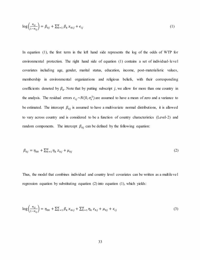
log (𝜋𝑖𝑗

1−𝜋𝑖𝑗) = 𝛽0𝑗 + ∑ 𝛽𝑘

𝐾𝑘=1 𝑥𝑘𝑖𝑗 + 𝜖𝑖𝑗 (1)

In equation (1), the first term in the left hand side represents the log of the odds of WTP for

environmental protection. The right hand side of equation (1) contains a set of individual- leve l

covariates including age, gender, marital status, education, income, post-materialistic values,

membership in environmental organizations and religious beliefs, with their corresponding

coefficients denoted by 𝛽𝑘 . Note that by putting subscript j, we allow for more than one country in

the analysis. The residual errors 𝜖𝑖𝑗 ~𝑁(0, 𝜎𝜖2) are assumed to have a mean of zero and a variance to

be estimated. The intercept 𝛽0𝑗 is assumed to have a multivariate normal distributions, it is allowed

to vary across country and is considered to be a function of country characteristics (Level-2) and

random components. The intercept 𝛽0𝑗 can be defined by the following equation:

𝛽0𝑗 = 휂00 + ∑ 휂𝑘𝐻ℎ=1 𝑧ℎ𝑗 + 𝜇0𝑗 (2)

Thus, the model that combines individual and country level covariates can be written as a multileve l

regression equation by substituting equation (2) into equation (1), which yields:

log (𝜋𝑖𝑗

1−𝜋𝑖𝑗) = 휂00 + ∑ 𝛽𝑘

𝐾𝑘 =1 𝑥𝑘𝑖𝑗 + ∑ 휂𝑘

𝐻ℎ=1 𝑧ℎ𝑗 + 𝜇0𝑗 + 𝜖𝑖𝑗 (3)

34

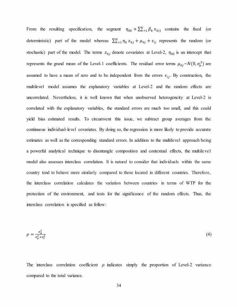
From the resulting specification, the segment 휂00 + ∑ 𝛽𝑘𝐾𝑘 =1 𝑥𝑘𝑖𝑗 contains the fixed (or

deterministic) part of the model whereas ∑ 휂𝑘𝐻ℎ=1 𝑧ℎ𝑗 + 𝜇0𝑗 + 휀𝑖𝑗 represents the random (or

stochastic) part of the model. The terms 𝑧ℎ𝑗 denote covariates at Level-2, 휂00 is an intercept that

represents the grand mean of the Level-1 coefficients. The residual error terms 𝜇0𝑗 ~𝑁(0, 𝜎𝜇2) are

assumed to have a mean of zero and to be independent from the errors 𝜖𝑖𝑗 . By construction, the

multilevel model assumes the explanatory variables at Level-2 and the random effects are

uncorrelated. Nevertheless, it is well known that when unobserved heterogeneity at Level-2 is

correlated with the explanatory variables, the standard errors are much too small, and this could

yield bias estimated results. To circumvent this issue, we subtract group averages from the

continuous individual- level covariates. By doing so, the regression is more likely to provide accurate

estimates as well as the corresponding standard errors. In addition to the multilevel approach being

a powerful analytical technique to disentangle composition and contextual effects, the multileve l

model also assesses interclass correlation. It is natural to consider that individuals within the same

country tend to behave more similarly compared to those located in different countries. Therefore,

the interclass correlation calculates the variation between countries in terms of WTP for the

protection of the environment, and tests for the significance of the random effects. Thus, the

interclass correlation is specified as follow:

𝜌 =𝜎𝜇

2

𝜎𝜇2 +𝜎𝜖

2 (4)

The interclass correlation coefficient 𝜌 indicates simply the proportion of Level-2 variance

compared to the total variance.

35

1.4. Data

1.4.1. The World Values Survey

The individual level data used in this study are from the WVS. The WVS is an investigat ion of basic

values and beliefs of the general public in a large number of countries and regions. The fifth wave

is more comprehensive than previous waves, it covers all regions and levels of development - high-

income, upper middle income, lower middle income and low-income countries. The fifth wave took

place in 59 countries and regions, and was carried out between 2005 and 2008. Appendix A provides

the year in which the survey was conducted for each country. A total of 83,975 individuals aged 15

years and above were interviewed. Personal information on socio-demographic characterist ics,

income, cultural and beliefs, and perception about environmental problems were gathered from

individuals in the participating countries and regions. The fifth wave is based on representative and

sufficiently large samples. Another advantage of the fifth wave, is that it includes many socio-

economic and demographic variables. We use it as a rich source of supplementary independent

variables to investigate in detail what shapes individuals to be concerned with environmental issues.

Among the questions asked in the fifth wave, there are numerous items that measure environmenta l

concern. However, for the purpose of this research, we analyse responses from two questions

included in the survey. That being said, in some part of the survey questionnaire, the respondents

were asked to state their WTP to prevent environmental pollution.

The exact wording is “I am now going to read out some statements about the environment. For each

one I read out, can you tell me whether you strongly agree, agree, disagree, or strongly disagree.

(1) I would be willing to give part of my income if I were sure that the money would be used

to prevent environmental pollution.

36

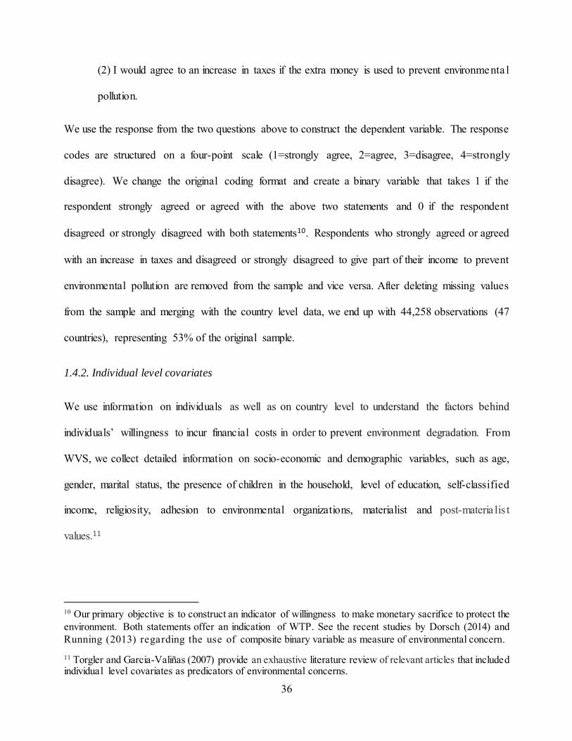
(2) I would agree to an increase in taxes if the extra money is used to prevent environmenta l

pollution.

We use the response from the two questions above to construct the dependent variable. The response

codes are structured on a four-point scale (1=strongly agree, 2=agree, 3=disagree, 4=strongly

disagree). We change the original coding format and create a binary variable that takes 1 if the

respondent strongly agreed or agreed with the above two statements and 0 if the respondent

disagreed or strongly disagreed with both statements10. Respondents who strongly agreed or agreed

with an increase in taxes and disagreed or strongly disagreed to give part of their income to prevent

environmental pollution are removed from the sample and vice versa. After deleting missing values

from the sample and merging with the country level data, we end up with 44,258 observations (47

countries), representing 53% of the original sample.

1.4.2. Individual level covariates

We use information on individuals as well as on country level to understand the factors behind

individuals’ willingness to incur financial costs in order to prevent environment degradation. From

WVS, we collect detailed information on socio-economic and demographic variables, such as age,

gender, marital status, the presence of children in the household, level of education, self-classified

income, religiosity, adhesion to environmental organizations, materialist and post-materia lis t

values.11

10 Our primary objective is to construct an indicator of willingness to make monetary sacrifice to protect the environment. Both statements offer an indication of WTP. See the recent studies by Dorsch (2014) and Running (2013) regarding the use of composite binary variable as measure of environmental concern. 11 Torgler and Garcia-Valiñas (2007) provide an exhaustive literature review of relevant articles that included individual level covariates as predicators of environmental concerns.

37

Considering age, it is argued that recent birth cohorts express higher levels of pro-

environmental behaviour and are more willing to contribute for its protection than older birth

cohorts, since older cohorts will not live long to enjoy the benefits of preserving resources for later

years (Dietz et al., 1998; Torgler and Garcia-Valiñas, 2007). Studies have also addressed the

differences between male and female in environmental concern (Bord and O’Connor, 1997;

Franzen and Meyer, 2010; McCright, 2010). These authors claim that in general women

show more willingness to contribute in monetary terms to protect the environment than men.

Zelezny and Yelverton (2000) have found that regardless of age, women are more willing to take

positive actions aiming at the protection of the environment than men. Furthermore, Hunter et al

(2004) provide valuable insights for the engagement of women in environmental protection.

They argue that the traditional gender socialization of women, the motherhood menta lity

and the ethics of care explain women’s engagement for the protection of the environment. In

contrast, Swallow et al (1994) and Cameron and Englin (1997) have found lower participation from

women.

Some studies explained the presence of children in the household as the reason why individuals are

more willing to pay to protect the environment. For instance, Laroche et al (2001) observe that

individua ls who are keener to pay for eco-friendly products are women, married, and have

at least one child. In short, it could be postulated that having children engenders social

responsibility (altruism) and enhances concern for the environment and thereby leads to

greater pro-environmental behaviour. Thus, we control for marital status and the presence

of children in the household. Regardless of age and gender, richer people are more likely to be

greener than poor people and are more willing to be concerned about the state of the environment

38

(Franzen and Meyer, 2010; Kemmelmeier et al., 2002; Franzen and Vogl, 2013). To test

this assertion, we control for relative income.

Besides controlling for important individual level characteristics such as age, gender and relative

income, studies also have shown that educated individua ls are more concerned about the

environment than non-educated ones, since they have better knowledge of environmenta l

problems (Olli et al., 2001). Subsequently, we investigate the effect of education on the

WTP to protect the environment. We also explore whether values and beliefs can affect

environmental concern. We used the scale that was developed by Inglehart (1990) as the measure

of post-materialistic values. Inglehart’s scale involves a battery of questions to measure value

orientations. Respondents were asked to determine what they believe to be the first and

second most important issues out of four choices:

(1) Maintaining order in the nation;

(2) Give people more say;

(3) Fighting rising prices; or

(4) Protecting freedom of speech.

Individuals are said to hold materialistic values when they have a combination of answers

(1) and (3), while individua ls are said to hold post-materialistic values when they answer

a combination (2) and (4). Individuals holding a mixture of materialistic a nd post-

materialistic values have a combination of answers (1) and (2) or a combination of answers

(3) and (4). It can also be argued that studies might be biased if the interviewed individua ls

seem to be environmental activists. To control for this type o f bias, we account for adhesion

39

to environmental movements.12 And finally, we investigate the effect of religiosity (or religious

beliefs) on environmental protection, since religion serves as an important source of morals to many

individuals around the globe.

1.4.3. Country level covariates

We merged individuals’ level data with data on country level. The country level data permits an

investigation into the differences in WTP to protect the environment across countries. Prior studies

have underlined the association between national wealth and environmental concern, and

revealed that higher income countries have on average, higher demand for a clean

environment (Gelissen, 2007; Franzen and Meyer, 2010; Knight and Messer, 2012). It has

been argued that wealthier nations have better quality of public mechanisms, which

contribute to individua ls’ wealth on top of their personal incomes and thereby increase

their WTP for the protection of the environment (Franzen and Meyer, 2010). To test the

effect of national wealth on the WTP for environmental protection, we consider the gross domestic

income per capita. Therefore, higher standards regarding environmental legislations and solid

institutions for the protection of the environment in developed countries may play a crucial role on

individuals’ involvement in the protection of the environment. Thus, we control for institut ions

quality (democracy and government stability). The local environmental quality condition is a

significant aspect to consider. Awareness of local environmental pollution such as, nitrous oxide

emissions, and of its negative impacts on humans’ health and ecosystem may influence individua l’s

action to contribute to improve local environmental problems. We also control for nitrous oxide

emissions (thousand metric tons of C02 equivalent per capita). It is expected that as a country

12 Adhesion to environmental organization is defined as being active or inactive member.

40

becomes more densely populated, environmental quality become of greater public concern. We

control for population density. Public spending could be a crucial aspect in explaining

individuals’ attitudes to contribute for environmental protection. Therefore, we include

government spending as a share of GDP to control for a country’s ability to deliver public

services to protect the environment. Except for the quality of institution which is from

International Country Risk Guide (ICRG) database, all the other variables are from the

World Development Indicators (World Bank). Table 1 provides a complete list of all variables

along with descriptive statistics. Panel A of Table 1 shows individual level characteristics while

Panel B provides statistics for the contextual covariates. Except for age and number of children, all

the individual level variables are specified as categorical variables whereas the contextual covariates

are continuous and averaged over 2005-2008. As can be seen, 65% of the World sample

population participants were ready to take action toward environmental protection. This distribution

is 70% for developing countries and 56% in the case of developed countries.13 The average age of

the whole sample was 41 with the target group being individuals of 15-98 years of age. In developing

countries the average age is 38 years, and 47 years in developed countries. The average number of

children in the household is comparable across groups of countries. Gender distribution of the

population is 50% and 52% female in developing and developed countries, respectively. Regarding

marital status, quite similar figures were observed among the group of individual classified as

(Married/Living as married). Individuals who have Incomplete/complete primary and

Incomplete/complete secondary education represent the largest group of educational attainment.

13 One plausible explanation for the higher WTP to support environmental protection in developing countries compared to developed countries could be that, in developing countries, the livelihood of the masses depends on the exploitation of natural resources (coal, oil and gas, agricultural and forest resources), the exploitation and processing of which results in local environment degradation, such as soil erosion, desertification, poor air and water quality, thereby leading to more support for the environment.

41

With respect to relative income, a great portion of individuals falls in the second and third quintile

categories. It is not surprising that there are more individuals possessing post-materialistic values in

developed countries than developing countries. Surprisingly, there are more individuals claiming to

be member of environmental organization in developing countries than developed countries. About

84% of individuals from developing world consider religion as important faith in their lives compare

with only 50% in developed countries. The bottom end of Table 1 provides summary statistics for

the country covariates used in the study. The higher the values for democracy and government

stability, the better the quality of institutions14.

14 Detailed definition of individuals and contextual variables are not presented to conserve space, but are available upon request.

42

Table 1. Descriptive statistics

Variables World Developed Developing Willingness to pay for environmental protection Yes 65.54% 55.99% 70.54% No 34.46% 44.01% 29.46% Panel A: Individual level covariates

Age 41.35 (SD=16.25) 46.90 SD=16.56) 38.44 (SD=15.31) Children 1.86 (SD=0.65) 1.80 (SD=0.54) 1.89 SD=0.70) Gender Female 50.80% 52.37% 49.97% Male 49.20% 47.63% 50.03% Marital Status Married/Living as married 64.02% 65.02% 63.50% Divorced/Separated/Widowed 24.98% 18.90% 28.17% Single/Never married 10.99% 16.08% 8.33% Educational level No formal education 7.79% 0.74% 11.49% Incomplete/complete primary 22.72% 18.57% 24.89% Incomplete/complete secondary 32.55% 35.34% 31.09% Incomplete/ complete university 36.94% 45.35% 32.53% Income Lower quintile 18.88% 17.20% 19.76% Second quintile 27.00% 27.14% 26.93% Third quintile 31.70% 28.78% 33.24% Fourth quintile 16.95% 17.32% 16.76% Upper quintile 5.46% 9.55% 3.31% Value Mixed 55.42% 57.62% 54.27% Materialist 33.47% 26.96% 36.87% Post-materialist 11.11% 15.42% 8.86% Membership of environmental organisation Member 13.03% 8.53% 15.38% Not a member 86.97% 91.47% 84.62% Religion Important 72.51% 49.71% 84.45% Not important 27.49% 50.29% 15.55% Individuals 44258 15216 29042 Panel B: Contextual level covariates Mean SD Mean SD Mean SD Log(Gross domestic income) 8.15 1.46 9.32 1.25 7.53 1.16 Log(NOx) 9.09 2.38 8.25 3.15 9.53 1.69 Democracy 4.72 1.40 5.69 0.53 4.21 1.45 Government stability 9.36 2.03 10.95 1.62 8.53 1.69 Government spending 27.80 10.44 38.88 5.74 22.01 7.15 Density 106.97 95.68 99.41 87.02 110.92 99.69 Countries 47 20 27

43

1.5. Results and discussion

1.5.1. Full sample of countries

Table 2 displays the estimated coefficients and the corresponding standard errors. Fixed effects are

reported in the upper part, while random effects are in the lower part of the table. As a first step, the

analysis begins by fitting an empty two-level model, that is, a model that contains only an intercept

and a random effect which allow the WTP to protect the environment to vary across countries as

specified in the model 015. The empty specification reveals that most of the variability in WTP to

protect the environment is originated in differences among individuals rather than between

countries. More accurately, the value of the interclass correlation shows that the country dimens ion

accounts for 19.5% of total variability. In other words, 80.5% of the variability in WTP to protect

the environment can be attributable to individuals’ level predictors. The findings indicate that

individuals’ level covariates play a more substantive role than contextual covariates in explaining

differences among individuals in WTP to protect the environment. Nonetheless, countries’

variability are not negligible and found to be also significant in explaining WTP to protect the

environment. To corroborate these findings, we perform a test of variance equality between

countries, the test rejects the null hypothesis that the between country variance is zero. Appendix B

shows the estimated residuals for all the 47 countries. We see that for a substantial number of

countries, the 95% confidence interval does not overlap the horizontal line at zero, indicating that

the WTP for environmental protection is significantly above or below the zero line which implies

quite a variation in terms of WTP across countries.

15 Models are fitted via adaptive numerical integration with seven quadrature points.

44

The inclusion of demographic variables (age, gender, children, marital status, education attainment

and income) brings changes to the model in terms of the estimate of the between-country variance.

The random intercept variance increases from 0.746 in model 0 to 0.810 in model 1. Thus, it can be

argued that the distribution of age, gender, children, marital status, education attainment and relative

income is different across countries. With regard to the estimated coefficients, the study reveals that

the effect of age on the log-odds of WTP to protect the environment is not statistically significant.

However, the study found that educated individuals are generally more supportive of the

environmental protection. This finding is in line with results reported in the literature regarding the

effect of formal education on willingness to contribute for the environment (Veisten et al, 2004;

Israel, D & Levinson, 2004). Wealthier individuals are found to be more willing to pay for the

protection of the environment than poor people. More importantly, we observe that the effect of

relative income on care for the environment increases linearly with income quintiles, suggesting that

wealthier individuals are gradually more likely to participate in the protection of the environment

than poorer individuals. Similar results were reported by Sulemana et al (2016b) who found that

relative to people who believe they are in the lower class, those in the working class, lower middle

class, upper middle class, and upper class tend to show significantly more environmental concern in

both African and developed countries. The study also suggest that the group of Single/Never married

and Divorced/Separated/Widowed are less caring for the environment than the group classified as

Married/Living as married. This is evidenced by the negative and significant value of the estimated

coefficients. As argued by Torgler and Garcia-Valiñas (2007) and Laroche et al (2001), married

people are more concerned about environmental degradation than others, because of their social

network and involvement in the community.

45

Furthermore, a bulk of the literature, however, has put forward values, religion and membership as

sources for the emergence of environmentalism (Kidd and Lee, 1997; Schultzet al, 2000; Franzen,

2003; Torgler and Garcia-Valiñas, 2007; Yuchtman-Yaar and Alkalay, 2007). It can be seen that

attitudes toward environmental protection differ substantially between post-materialistic and

materialistic individuals, between religious and secular and between membership of environmenta l

organization and non-member. Precisely, we found that post-materialistic individuals are more

likely to contribute to protecting the environment than those possessing materialistic values. Being

a member of environmental organization has a profound influence on the log-odds of WTP to protect

the environment. The need to protect the environment was also found to be stronger in faithful

individuals than those with secular behaviour.

It is highly possible that people with strong environmental preferences may choose to be members

of environmental organizations. This could lead to endogeneity. To control for such a problem,

values and membership have been removed in the last four estimations. The results remain robust

after removing these two variables.

Then, we attempted to capture country attributes that are likely to influence individuals’ decisions

on WTP to protect the environment. We used national income to assess whether affluence can

influence attitudes toward the environment. Nitrous oxide emissions was used as an indicator of the

local ecological footprint. Also, scholars have stressed the relationship between the quality of

institutions and environmental management (Paavola, 2007). Thus, we control for the level of

democracy and government stability. Finally, we also investigate the effect of population density on

the log-odds of the WTP to protect the environment.

Before including the aforementioned country level into the model, it is important to test the

appropriateness of multilevel modeling. Basically, there is no standard procedure for testing the

46

multilevel modeling structure of the data. However, in order to opt for the proper model, we perform

a likelihood ratio test between the multilevel model without contextual effects (constrained model)

and a model with contextual effects (unconstrained model). The likelihood ratio test clearly indicates

that the unconstrained model is the preferred model (Prob > χ2 = 0.0014). Thus, we proceed by

adding the contextual level variables into the model. It is interesting to see that the inclusion of the

country level covariates decreases the random intercept variance. It is expected that the variance

components would become smaller as relevant explanatory variables are included in the subsequent

models (Hox et al, 2010). Furthermore, the inclusion of country level variables substantially reduces

the interclass correlation by 4 to 6 percentage points.

With respect to the estimated coefficients, we observe that concerns for environmental protection is

more pronounced in developing countries than developed countries. Local environmental condition

and the density of population do not have influence on the log-odds of WTP to protect the

environment. Country wealth has a limited effect on the WTP to protect the environment. The study

found that the level of democracy as well as government stability is negatively associated with the

WTP to protect the environment. However, the study finds that government spending has no

statistically significant impact on individuals’ preferences for environmental protection.

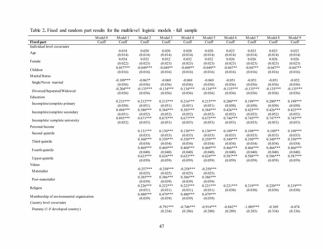
47

Table 2. Fixed and random part results for the multilevel logistic models - full sample Model 0 Model 1 Model 2 Model 3 Model 4 Model 5 Model 6 Model 7 Model 8 Model 9 Fixed part Coeff Coeff Coeff Coeff Coeff Coeff Coeff Coeff Coeff Coeff Individual level covariates

Age 0.018 (0.014)

0.020 (0.014)

0.020 (0.014)

0.020 (0.014)

0.020 (0.014)

0.023 (0.014)

0.023 (0.014)

0.023 (0.014)

0.023 (0.014)

Female 0.034 (0.022)

0.032 (0.023)

0.032 (0.023)

0.032 (0.023)

0.032 (0.023)

0.026 (0.023)

0.026 (0.023)

0.026 (0.023)

0.026 (0.023)

Children 0.057*** (0.016)

-0.049*** (0.016)

-0.049** (0.016)

-0.049** (0.016)

-0.049** (0.016)

-0.047** (0.016)

-0.047** (0.016)

-0.047** (0.016)

-0.047** (0.016)

Marital Status

Single/Never married -0.109*** (0.036)

-0.067* (0.036)

-0.069 (0.036)

-0.069 (0.036)

-0.069 (0.036)

-0.051 (0.036)

-0.051 (0.036)

-0.051 (0.036)

-0.052 (0.036)

Divorced/Separated/Widowed -0.204*** (0.036)

-0.135*** (0.036)

-0.134*** (0.036)

0.134*** (0.036)

-0.134*** (0.036)

-0.135*** (0.036)

-0.135*** (0.036)

-0.135*** (0.036)

-0.135*** (0.036)

Education

Incomplete/complete primary 0.233*** (0.050)

0.212*** (0.051)

0.215*** (0.051)

0.216*** (0.051)

0.215*** (0.051)

0.200*** (0.050)

0.199*** (0.050)

0.200*** (0.050)

0.199*** (0.050)

Incomplete/complete secondary 0.494*** (0.051)

0.380*** (0.052)

0.384*** (0.052)

0.385*** (0.052)

0.384*** (0.052)

0.426*** (0.052)

0.425*** (0.052)

0.426*** (0.052)

0.425*** (0.052)

Incomplete/ complete university 0.893*** (0.052)

0.671*** (0.053)

0.675*** (0.053)

0.677*** (0.053)

0.675*** (0.053)

0.746*** (0.053)

0.745*** (0.053)

0.747*** (0.053)

0.745*** (0.053)

Personal Income

Second quintile 0.131*** (0.033)

0.130*** (0.033)

0.130*** (0.033)

0.130*** (0.033)

0.109*** (0.033)

0.109*** (0.033)

0.109** (0.033)

0.109*** (0.033)

Third quintile 0.360*** (0.034)

0.359*** (0.034)

0.358*** (0.034)

0.359*** (0.034)

0.349*** (0.034)

0.350*** (0.034)

0.349*** (0.034)

0.350*** (0.034)

Fourth quintile 0.469*** (0.040)

0.469*** (0.040)

0.468*** (0.040)

0.469*** (0.040)

0.466*** (0.040)

0.466*** (0.040)

0.466*** (0.040)

0.466*** (0.040)

Upper quintile 0.623*** (0.059)

0.624*** (0.059)

0.623*** (0.059)

0.624*** (0.059)

0.587*** (0.059)

0.588*** (0.059)

0.586*** (0.059)

0.587*** (0.059)

Values

Materialist -0.257*** (0.025)

-0.258*** (0.025)

-0.258*** (0.025)

-0.258*** (0.025)

Post-materialist 0.385*** (0.039)

0.386*** (0.039)

0.386*** (0.039)

0.386*** (0.039)

Religion 0.226*** (0.031)

0.222*** (0.031)

0.223*** (0.031)

0.221*** (0.031)

0.221*** (0.030)

0.219*** (0.030)

0.220*** (0.030)

0.219*** (0.030)

Membership of environmental organization 0.480*** (0.039)

0.479*** (0.039)

0.480*** (0.039)

0.479*** (0.039)

Country level covariates

Dummy (1 if developed country) -0.791*** (0.234)

-0.746*** (0.286)

-0.914*** (0.280)

-0.842** (0.289)

-1.005*** (0.283)

-0.369 (0.334)

-0.474 (0.336)

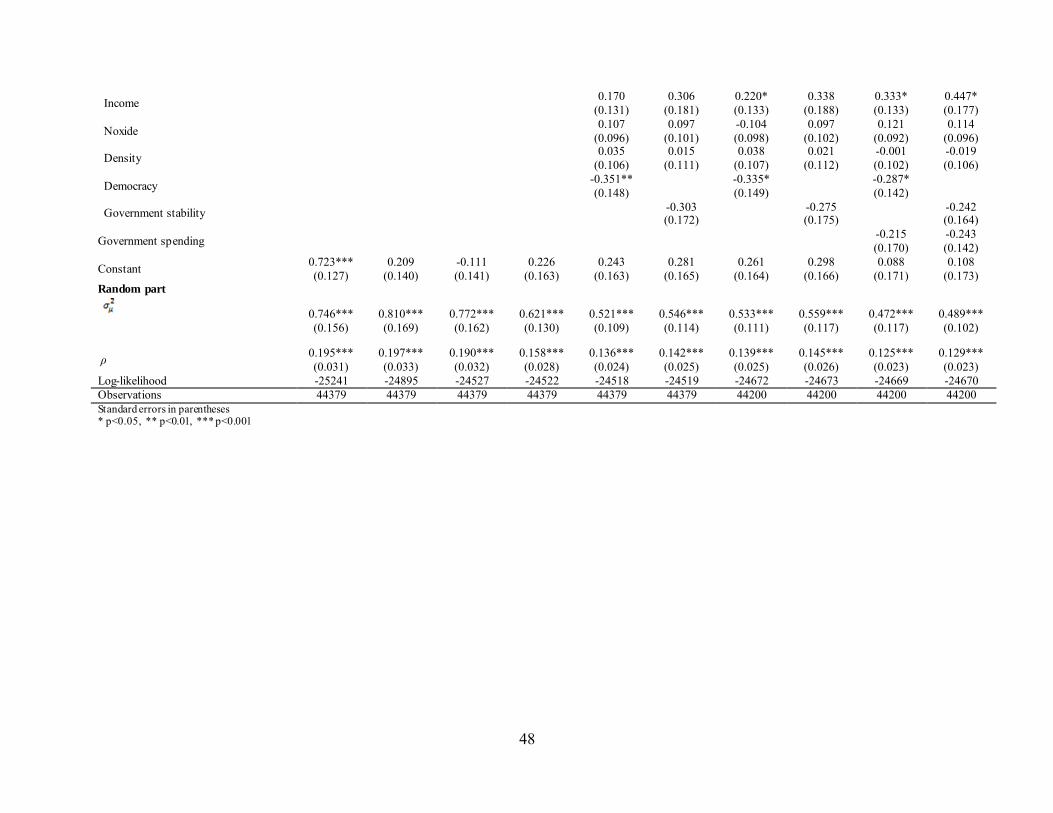
48

Income 0.170 (0.131)

0.306 (0.181)

0.220* (0.133)

0.338 (0.188)

0.333* (0.133)

0.447* (0.177)

Noxide 0.107 (0.096)

0.097 (0.101)

-0.104 (0.098)

0.097 (0.102)

0.121 (0.092)

0.114 (0.096)

Density 0.035 (0.106)

0.015 (0.111)

0.038 (0.107)

0.021 (0.112)

-0.001 (0.102)

-0.019 (0.106)

Democracy -0.351** (0.148)

-0.335* (0.149)

-0.287* (0.142)

Government stability -0.303 (0.172)

-0.275 (0.175)

-0.242 (0.164)

Government spending -0.215 (0.170)

-0.243 (0.142)

Constant 0.723*** (0.127)

0.209 (0.140)

-0.111 (0.141)

0.226 (0.163)

0.243 (0.163)

0.281 (0.165)

0.261 (0.164)

0.298 (0.166)

0.088 (0.171)

0.108 (0.173)

Random part

0.746*** (0.156)

0.810*** (0.169)

0.772*** (0.162)

0.621*** (0.130)

0.521*** (0.109)

0.546*** (0.114)

0.533*** (0.111)

0.559*** (0.117)

0.472*** (0.117)

0.489*** (0.102)

ρ 0.195*** (0.031)

0.197*** (0.033)

0.190*** (0.032)

0.158*** (0.028)

0.136*** (0.024)

0.142*** (0.025)

0.139*** (0.025)

0.145*** (0.026)

0.125*** (0.023)

0.129*** (0.023)

Log-likelihood -25241 -24895 -24527 -24522 -24518 -24519 -24672 -24673 -24669 -24670 Observations 44379 44379 44379 44379 44379 44379 44200 44200 44200 44200 Standard errors in parentheses * p<0.05, ** p<0.01, *** p<0.001

49

1.5.2. Developed countries

The evidence provided so far has been obtained for the full sample of countries. But, it can be argued

that the effect of individuals and, particularly, that of countries are likely to vary between groups of

countries. As such, we present subsequently the results obtained for developed and developing

countries. Table 3 gives the results for developed countries. The findings reported in Model 0

indicate that the random intercept variance is 0.316 and the corresponding interclass correlation is

0.087, meaning that about 9% of total variability of the WTP to protect the environment can be

attributable to countries level predictors in developed countries. As opposed to the results observed

for the full sample of countries, the effect of age was found to be positive and statistically significant

across all specification, signaling that older individuals are significantly more likely to agree to give

part of their income for the protection of the environment. We found no evidence in gender

difference with regard to WTP to protect the environment, which contradicts the results found by

Torgler et al. (2008) indicating that women have both a stronger preference towards the environment

and a stronger willingness to contribute. With respect to the effect of children on WTP to protect

the environment, we found that individuals that have children are less likely to contribute to improve

the quality of the environment in developed countries. The study also found correlation between

individual’s education and willingness to make income sacrifices to prevent environmenta l

pollution. Individuals who have attained secondary and university education are more likely to agree

to give part of their income for the protection of the environment in developed countries. It can be

disputed that educated people are able to understand the harmful effects of pollution on the

environment and are more willing to advocate for a clean environment. The effect of relative income

on individuals’ WTP was as expected, with higher relative income being associated with higher log

odds of WTP to protect the environment. This association was statistically significant for all

50

quintiles and consistent with previous findings by Sulemana et al (2016b). The findings also reveal

religion and being a member of an environmental organization matter for the willingness to give

part of one’s income for environmental protection. Those who hold post-materialistic values are

more likely to agree to give part of their income among individuals of developed countries.

Additionally, the results reported in Model 3 and 4 reveal that country’s wealth has a significant

influence on the log-odds of WTP to protect the environment. Individuals living in democratic and

stable government are less likely to contribute for improvements to the quality of the environment.

It could be argued that in developed countries, stability and predictability of the political and

regulatory environment as well as good administrative conditions are favorable to implement

environmental taxation. These tax compliance give rise to low incentives for individuals to

contribute for preventing environmental damage. A possible explanation for the low WTP might be,

people believe that government should address environmental issues and it is not necessary to pay

additional taxes for environmental protection.

Population density has significant influence while local environment conditions do not have

significant effect on individuals’ WTP to protect the environment in developed countries.

51

Table 3. Fixed and random part results for the multilevel logistic models – developed countries

Model 0 Model 1 Model 2 Model 3 Model 4 Model 5 Model 6 Model 7 Model 8 Fixed part Coeff Coeff Coeff Coeff Coeff Coeff Coeff Coeff Coeff Individual level covariates

Age 0.041* (0.021)

0.062** (0.022)

0.062** (0.022)

0.062*** (0.022)

0.071** (0.022)

0.070** (0.022)

0.072*** (0.022)

0.071** (0.022)

Female -0.009 (0.035)

-0.002 (0.036)

-0.002 (0.036)

-0.002 (0.036)

0.019 (0.036)

0.021 (0.037)

0.019 (0.036)

0.020 (0.036)

Children -0.055** (0.023)

-0.043 (0.024)

-0.044 (0.024)

-0.043 (0.024)

-0.038 (0.024)

-0.038 (0.024)

-0.038 (0.024)

-0.038 (0.024)

Marital Status

Single/Never married -0.025 (0.059)

0.068 (0.060)

0.068 (0.060)

0.068 (0.060)

0.081 (0.060)

0.081 (0.060)

0.081 (0.060)

0.081 (0.060)

Divorced/Separated/Widowed -0.146** (0.050)

-0.039 (0.052)

-0.038 (0.052)

-0.037 (0.052)

-0.040 (0.052)

-0.039 (0.052)

-0.040 (0.052)

-0.039 (0.052)

Education

Incomplete/complete primary 0.275 (0.210)

0.253 (0.214)

0.252 (0.214)

0.252 (0.214)

0.228 (0.211)

0.228 (0.211)

0.227 (0.211)

0.226 (0.211)

Incomplete/complete secondary 0.570** (0.209)

0.435* (0.213)

0.434* (0.212)

0.432** (0.212)

0.486* (0.210)

0.485* (0.210)

0.486* (0.210)

0.484* (0.210)

Incomplete/ complete university 1.122*** (0.209)

0.843*** (0.213)

0.840*** (0.213)

0.837*** (0.213)

0.934*** (0.211)

0.932*** (0.211)

0.934*** (0.211)

0.931*** (0.211)

Personal Income

Second quintile 0.222*** (0.055)

0.223*** (0.055)

0.225*** (0.055)

0.258*** (0.054)

0.259*** (0.054)

0.258*** (0.054)

0.259*** (0.054)

Third quintile 0.402*** (0.057)

0.404*** (0.057)

0.406*** (0.057)

0.445*** (0.056)

0.446*** (0.056)

0.445*** (0.056)

0.447*** (0.056)

Fourth quintile 0.586*** (0.065)

0.585*** (0.065)

0.587*** (0.065)

0.677*** (0.064)

0.679*** (0.064)

0.677*** (0.064)

0.679*** (0.064)

Upper quintile 0.659*** (0.081)

0.656*** (0.081)

0.658*** (0.081)

0.666*** (0.080)

0.668*** (0.080)

0.667*** (0.080)

0.669*** (0.080)

Values

Materialist -0.246*** (0.042)

-0.244*** (0.043)

-0.245*** (0.042)

Post-materialist 0.528*** (0.055)

0.527*** (0.055)

0.528*** (0.055)

Religion 0.152*** (0.040)

0.156*** (0.040)

0.152*** (0.040)

0.156*** (0.039)

0.153*** (0.039)

0.156*** (0.039)

0.153*** (0.039)

Membership of environmental organization 0.632*** (0.073)

0.631*** (0.073)

0.633*** (0.073)

Country level covariates

Income 0.261*** (0.092)

0.509*** (0.122)

0.315*** (0.095)

0.538*** (0.130)

0.295** (0.100)

0.526*** (0.125)

52

Noxide 0.030 (0.149)

0.041 (0.127)

0.006 (0.156)

-0.049 (0.135)

-0.015 (0.159)

-0.088 (0.134)

Density 0.269*** (0.096)

0.313*** (0.108)

-0.170 (0.110)

-0.300** (0.115)

-0.165 (0.110)

-0.307** (0.111)

Democracy -0.657** (0.282)

-0.520 (0.292)

-0.525 (0.289)

Government stability -0.434*** (0.123)

-0.377** (0.130)

-0.411** (0.128)

Government spending -0.110 (0.126)

-0.212 (0.128)

Constant 0.306* (0.127)

-0.433 (0.241)

-0.751*** (0.245)

-0.554 (0.288)

-0.910*** (0.240)

-0.764** (0.291)

-1.047*** (0.239)

-0.861** (0.333)

-1.240*** (0.283)

Random part

0.316*** (0.101)

0.282*** (0.091)

0.261*** (0.084)

0.169*** (0.055)

0.132*** (0.043)

0.182** (0.059)

0.148** (0.048)

0.179** (0.058)

0.137** (0.045)

ρ 0.087*** (0.025)

0.079*** (0.023)

0.073*** (0.022)

0.049*** (0.015)

0.038*** (0.012)

0.052** (0.016)

0.043** (0.013)

0.051** (0.016)

0.040** (0.012)

Log-likelihood -9778 -9585 -9392 -9388 -9386 -9478 -9476 -9478 -9475 Observations 15225 15225 15225 15225 15225 15156 15156 15156 15156 Standard errors in parentheses * p<0.05, ** p<0.01, *** p<0.001

53

1.5.3. Developing countries

Table 4 gives the results for developing countries. The intercept-only model was tried first (as

reported in Model 0). The interclass correlation reported in Model 0 shows that country level

covariates play a non-negligible role in determining the probability of contributing to improve the

quality of the environment. After adjustment for individuals level variables (reported in Model 1),

results show that most of the potential predictors considered were found to have a significant

association with WTP to protect the environment. Overall, although previous studies have identified

females with children as being more willing to pay for environmentally friendly products

(Thompson, 1998, Laroche et al, 2001), we found that individuals that have children exhibit less

pro-environmental intentions. Being female or male does not have impact on the log-odds of WTP

to protect the environment. The regression result shows a negative and significant role for the group

of Single/Never married and Separated/divorced/widowed, which suggest that Single/Never married

and the segment of marital status Separated/divorced/widowed tend to contribute less for the

protection of the environment compared with the group married/ and live as married couple. As

expected, educated individuals are more likely to be concerned and willing to pay for the protection

of the environment than their non-educated counterparts.

Environmental consciousness is related to individuals’ perceptions about their beliefs and values. In

line with the literature discussed in the previous section, individuals possessing post-materialist ic

values tend to engage more in the protection of the environment (see results in Model 2). In contrast,

those possessing materialistic values are less worried about environmental issues. Result found that

faithful individuals are more concerned about environmental issues. Unsurprisingly, members of

environmental organization are more likely to show care for the environment than non-members.

54

The positive effect of members of environmental organization on environmental concern remains

strong and highly significant across all model specifications.

Then, we introduced Income, Nitrous oxide, Density, Democracy and Government stability (As in

Model 3 and of Table 4). As can be seen, a rise in government stability reduces the proportion of

individuals willing to give part of their income to prevent environmental pollution. The remaining

contextual variables do not have significant impact on the individuals’ willingness to prevent

environment pollution. It is important to note that the random intercept variance as well as the

interclass correlation are relatively constant across the estimated models.

55

Table 4. Fixed and random part results for the multilevel logistic models – developing countries

Model 0 Model 1 Model 2 Model 3 Model 4 Model 5 Model 6 Model 7 Model 8 Fixed part coeff coeff coeff coeff coeff coeff coeff coeff coeff Individual level covariates

Age 0.009 (0.019)

0.001 (0.019)

0.001 (0.019)

0.002 (0.019)

0.002 (0.019)

0.002 (0.019)

0.002 (0.019)

0.002 (0.019)

Female 0.056 (0.029)

0.047 (0.029)

0.047 (0.029)

0.047 (0.029)

0.025 (0.029)

0.025 (0.029)

0.025 (0.029)

0.025 (0.029)

Children -0.058** (0.021)

-0.050* (0.021)

-0.050* (0.021)

-0.050* (0.021)

-0.052* (0.021)

-0.052* (0.021)

-0.053* (0.021)

-0.053* (0.021)

Marital Status (Married=Ref.)

Single/Never married -0.148** (0.045)

-0.137** (0.046)

-0.137** (0.046)

-0.137** (0.046)

-0.110* (0.045)

-0.110* (0.045)

-0.111* (0.045)

-0.111* (0.045)

Divorced/Separated/Widowed -0.246*** (0.052)

-0.207*** (0.052)

-0.207*** (0.052)

-0.207*** (0.052)

-0.207*** (0.052)

-0.207*** (0.052)

-0.207*** (0.052)

-0.207*** (0.052)

Education (No education=Ref.)

Incomplete/complete primary 0.261*** (0.053)

0.227*** (0.054)

0.228*** (0.054)

0.228*** (0.054)

0.222*** (0.054)

0.222*** (0.054)

0.222*** (0.054)

0.221*** (0.054)

Incomplete/complete secondary 0.535*** (0.055)

0.422*** (0.056)

0.423*** (0.056)

0.424*** (0.056)

0.460*** (0.056)

0.460*** (0.056)

0.459*** (0.056)

0.459*** (0.056)

Incomplete/ complete university 0.797*** (0.057)

0.604*** (0.059)

0.606*** (0.059)

0.605*** (0.059)

0.661*** (0.058)

0.661*** (0.058)

0.661*** (0.058)

0.661*** (0.058)

Personal Income (First quintile=Ref.)

Second quintile 0.084* (0.041)

0.084* (0.041)

0.084* (0.041)

0.029 (0.041)

0.030 (0.041)

0.029 (0.041)

0.029 (0.041)

Third quintile 0.350*** (0.043)

0.349*** (0.043)

0.350*** (0.043)

0.308*** (0.042)

0.309*** (0.042)

0.307*** (0.042)

0.308*** (0.042)

Fourth quintile 0.409*** (0.052)

0.408*** (0.052)

0.409*** (0.052)

0.340** (0.052)

0.340** (0.052)

0.338*** (0.052)

0.339** (0.052)

Upper quintile 0.626*** (0.094)

0.625*** (0.094)

0.626*** (0.094)

0.570*** (0.093)

0.571*** (0.093)

0.570*** (0.093)

0.570*** (0.093)

Values (Mixed=Ref.)

Materialist -0.272*** (0.030)

-0.272*** (0.030)

-0.272*** (0.030)

Post-materialist 0.211*** (0.056)

0.211*** (0.056)

0.211*** (0.056)

Religion 0.338*** (0.049)

0.339*** (0.049)

0.337*** (0.049)

0.323*** (0.049)

0.320*** (0.049)

0.323*** (0.049)

0.320*** (0.049)

Membership of environmental organization 0.412*** (0.046)

0.412*** (0.046)

0.410*** (0.046)

Country level covariates

Income -0.066 (0.466)

-0.063 (0.454)

-0.115 (0.466)

-0.083 (0.450)

0.933 (0.531)

0.710 (0.515)

56

Noxide -0.110 (0.124)

-0.014 (0.140)

-0.103 (0.125)

0.001 (0.140)

-0.192 (0.112)

0.117 (0.134)

Density 0.134 (0.157)

0.173 (0.155)

0.140 (0.157)

0.179 (0.154)

0.032 (0.140)

0.077 (0.144)

Democracy -0.290 (0.196)

-0.275 (0.195)

-0.294 (0.169)

Government stability -0.583 (0.348)

-0.615 (0.345)

0.415 (0.321)

Government spending -0.352 (0.281)

-0.137 (0.296)

Constant 1.031*** (0.178)

0.590** (0.187)

0.208 (0.195)

0.132 (0.263)

-0.011 (0.263)

0.127 (0.263)

-0.016 (0.260)

0.114 (0.229)

-0.001 (0.236)

Random part

0.844*** (0.232)

0.849*** (0.239)

0.883*** (0.243)

0.837*** (0.202)

0.720*** (0.198)

0.737*** (0.202)

0.706*** (0.195)

0.548*** (0.151)

0.572*** (0.158)

ρ 0.204*** (0.044)

0.208*** (0.045)

0.211*** (0.045)

0.193*** (0.041)

0.179*** (0.040)

0.183*** (0.041)

0.176*** (0.040)

0.142*** (0.033)

0.148*** (0.035)

Log-likelihood -15456 -15278 -15084 -15082 -15081 -15151 -15151 -15147 -15148 Observations 29154 29154 29154 29154 29154 29044 29044 29044 29044 Standard errors in parentheses * p<0.05, ** p<0.01, *** p<0.001

57

1.5.4. Robustness analysis of the results

In this subsection, we examine the robustness of our results by testing an alternative specificat ion

of the dependent variable. Recall that the analysis in this study proceeds by merging responses from

the two aforementioned environment-related questions to construct a binary dependent variable and

applying a multilevel logit model to investigate the WTP to prevent environmental pollution. To

test robustness, we analysed each question separately by running a multilevel ordered logit model.

The results from this exercise are presented in Table 5. The results are broadly in line with results

obtained with the multilevel logit model. Similar to the multilevel logit model results, we found that

the WTP to prevent environmental pollution is higher (from strongly disagree to strongly agree)

with higher age, higher level of education, increase in income, post-materialistic values and religious

beliefs. In other words, respondents in the lower category (e.g., strongly agree) are more likely to

pay to prevent environmental pollution. The results are consistent across developed and developing

countries. These observations demonstrate the robustness of the results.

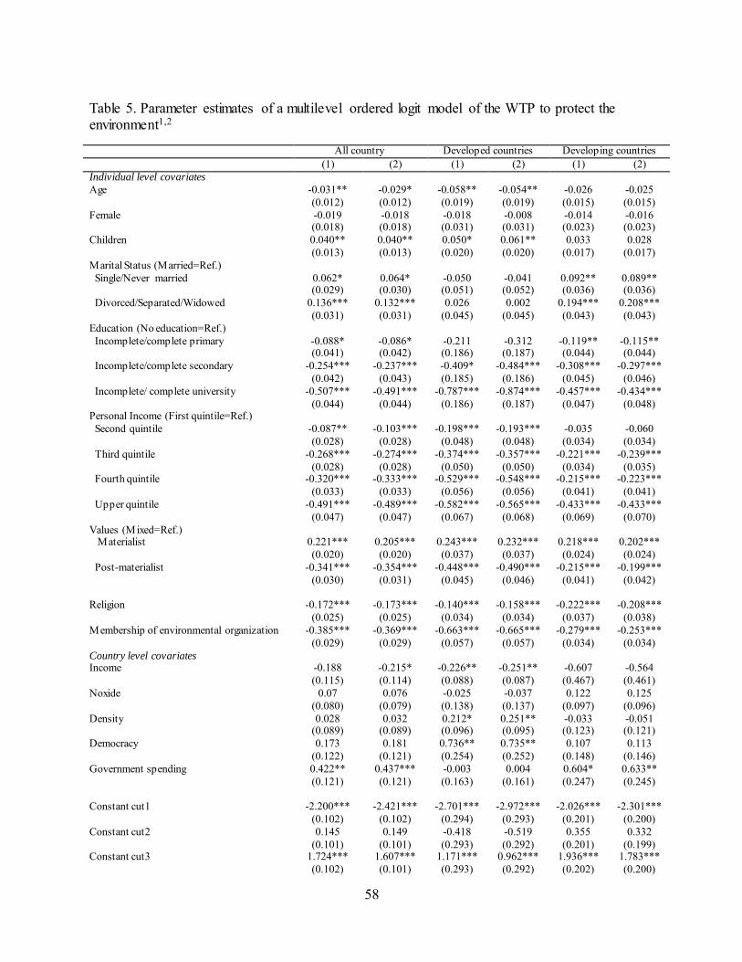
58

Table 5. Parameter estimates of a multilevel ordered logit model of the WTP to protect the environment1,2 All country Developed countries Developing countries (1) (2) (1) (2) (1) (2) Individual level covariates Age -0.031** -0.029* -0.058** -0.054** -0.026 -0.025 (0.012) (0.012) (0.019) (0.019) (0.015) (0.015) Female -0.019 -0.018 -0.018 -0.008 -0.014 -0.016 (0.018) (0.018) (0.031) (0.031) (0.023) (0.023) Children 0.040** 0.040** 0.050* 0.061** 0.033 0.028 (0.013) (0.013) (0.020) (0.020) (0.017) (0.017) Marital Status (Married=Ref.) Single/Never married 0.062* 0.064* -0.050 -0.041 0.092** 0.089** (0.029) (0.030) (0.051) (0.052) (0.036) (0.036) Divorced/Separated/Widowed 0.136*** 0.132*** 0.026 0.002 0.194*** 0.208*** (0.031) (0.031) (0.045) (0.045) (0.043) (0.043) Education (No education=Ref.) Incomplete/complete primary -0.088* -0.086* -0.211 -0.312 -0.119** -0.115** (0.041) (0.042) (0.186) (0.187) (0.044) (0.044) Incomplete/complete secondary -0.254*** -0.237*** -0.409* -0.484*** -0.308*** -0.297*** (0.042) (0.043) (0.185) (0.186) (0.045) (0.046) Incomplete/ complete university -0.507*** -0.491*** -0.787*** -0.874*** -0.457*** -0.434*** (0.044) (0.044) (0.186) (0.187) (0.047) (0.048) Personal Income (First quintile=Ref.) Second quintile -0.087** -0.103*** -0.198*** -0.193*** -0.035 -0.060 (0.028) (0.028) (0.048) (0.048) (0.034) (0.034) Third quintile -0.268*** -0.274*** -0.374*** -0.357*** -0.221*** -0.239*** (0.028) (0.028) (0.050) (0.050) (0.034) (0.035) Fourth quintile -0.320*** -0.333*** -0.529*** -0.548*** -0.215*** -0.223*** (0.033) (0.033) (0.056) (0.056) (0.041) (0.041) Upper quintile -0.491*** -0.489*** -0.582*** -0.565*** -0.433*** -0.433*** (0.047) (0.047) (0.067) (0.068) (0.069) (0.070) Values (Mixed=Ref.) Materialist 0.221*** 0.205*** 0.243*** 0.232*** 0.218*** 0.202*** (0.020) (0.020) (0.037) (0.037) (0.024) (0.024) Post-materialist -0.341*** -0.354*** -0.448*** -0.490*** -0.215*** -0.199*** (0.030) (0.031) (0.045) (0.046) (0.041) (0.042) Religion -0.172*** -0.173*** -0.140*** -0.158*** -0.222*** -0.208*** (0.025) (0.025) (0.034) (0.034) (0.037) (0.038) Membership of environmental organization -0.385*** -0.369*** -0.663*** -0.665*** -0.279*** -0.253*** (0.029) (0.029) (0.057) (0.057) (0.034) (0.034) Country level covariates Income -0.188 -0.215* -0.226** -0.251** -0.607 -0.564 (0.115) (0.114) (0.088) (0.087) (0.467) (0.461) Noxide 0.07 0.076 -0.025 -0.037 0.122 0.125 (0.080) (0.079) (0.138) (0.137) (0.097) (0.096) Density 0.028 0.032 0.212* 0.251** -0.033 -0.051 (0.089) (0.089) (0.096) (0.095) (0.123) (0.121) Democracy 0.173 0.181 0.736** 0.735** 0.107 0.113 (0.122) (0.121) (0.254) (0.252) (0.148) (0.146) Government spending 0.422** 0.437*** -0.003 0.004 0.604* 0.633** (0.121) (0.121) (0.163) (0.161) (0.247) (0.245) Constant cut1 -2.200*** -2.421*** -2.701*** -2.972*** -2.026*** -2.301*** (0.102) (0.102) (0.294) (0.293) (0.201) (0.200) Constant cut2 0.145 0.149 -0.418 -0.519 0.355 0.332 (0.101) (0.101) (0.293) (0.292) (0.201) (0.199) Constant cut3 1.724*** 1.607*** 1.171*** 0.962*** 1.936*** 1.783*** (0.102) (0.101) (0.293) (0.292) (0.202) (0.200)

59

Var (Constant) 0.362*** 0.357*** 0.137*** 0.135*** 0.425*** 0.415*** (0.076) (0.075) (0.045) (0.044) (0.117) (0.114) Log-likelihood -51992 -51032 -18408 -18151 -33492 -32761 Observations 44379 44379 15225 15225 29154 29154 Standard errors in parentheses * p<0.05, ** p<0.01, *** p<0.001 (1). Would give part of my income for environment (1=strongly agree, 2=agree, 3=disagree, 4=strongly disagree). (2). Increase in taxes if extra money used to prevent environment (1=strongly agree, 2=agree, 3=disagree, 4=strongly disagree).

1.6. Conclusions

This chapter investigates individual characteristics and contextual covariates guiding individua ls

toward environmental protection. It uses survey data from the fifth wave of WVS and country level

data from the World Development Indicators database and applies a two level logist ic

regression to determine what shapes individual environmental concern. Overall, the study find that

individual level covariates accounts for 80.5% of total variability in explaining environmenta l

awareness across nations. The remaining 19.5% is attributable to country level characteristics. The

commonly used individual level predicators such as education, relative income, post-materialist ic

values, religious beliefs and adhesion to environmental organization are found to be consistent ly

associated with individuals’ preference to incur financial cost in order to protect the environment.

These results are in line with the findings reported in much of the literature dealing with

determinants of environmental concern.

Although the results show that individual level characteristics play a significant role in explaining

the WTP to protect the environment, contextual factors are also found to be non-negligible in

explaining individuals’ preferences towards environmental protection. The study reveals that

country’s wealth has a significant impact on individuals’ willingness to give part of their income

and agreeing to an increase in taxes to prevent environmental pollution. Furthermore, we observe

that population density has an influence on individuals’ environmental preferences mainly in

developed countries. However, an aspect which has been overwhelmingly overlooked in the

60

environmental literature is the effect of the quality of institutions on individuals’ preference to pay

money for the protection of the environment.

To assess the effect of the quality of institutions on individuals’ preference, we use democracy and

government stability as indicators. We observe that both democracy and government stability reduce

individuals’ intention to give part of their income and agreeing to an increase in taxes to prevent

environmental pollution mainly in developed countries. This result remains robust after controlling

for other contextual factors.

In sum, the findings from this study reveals that the disparities in the WTP to protect the environment

between countries can be originated from both individual and country level covariates. Therefore,

to better understand the factors behind individuals in relation to environmental prevention, it

important to consider the economic condition and the quality of institutions of the country in which

the individual is located. All these factors play an important role in defining the individua l’s

engagement in environmental prevention.

61

Appendix A: List of countries included in the analysis

Country/Region Survey year Respondents Developed/developing countries

Andorra 2005 769 1 Australia 2005 897 1 Brazil 2006 1,031 0 Bulgaria 2005 626 1 Burkina Faso 2007 867 0 Canada 2005 1,310 1 Chile 2006 668 0 China 2007 1,689 0 Cyprus 2006 815 0 Egypt 2008 2,244 0 Ethiopia 2007 1,137 0 Finland 2005 682 1 Georgia 2008 803 0 Germany 2006 1,332 1 Ghana 2007 1,116 0 Hungary 2008 665 1 India 2006 955 0 Indonesia 2006 1,102 0 Iran 2005 2,064 0 Italy 2005 483 1 Japan 2005 499 1 Jordan 2007 782 0 Malaysia 2006 840 0 Mali 2007 683 0 Mexico 2005 1,029 0 Moldova 2006 758 1 Morocco 2007 715 0 New Zealand 2005 390 1 Norway 2007 766 1 Peru 2006 946 0 Poland 2005 657 1 Romania 2005 1,141 1 Rwanda 2007 1,111 0 Serbia and Montenegro 2005 685 1 Slovenia 2005 646 1 South Africa 2006 2,082 0 South Korea 2005 780 0 Spain 2007 815 1 Sweden 2006 706 1 Switzerland 2007 762 1 Thailand 2007 1,141 0 Trinidad and Tobago 2006 733 0 Turkey 2007 1,072 0 Ukraine 2006 627 1 Uruguay 2006 630 0 Viet Nam 2006 1,264 0 Zambia 2007 743 0 Countries are classified according to macro geographical regions and sub-regions, and selected economic and other groupings (the United Nations Statistics Division), China includes Taiwan, developed countries =1.

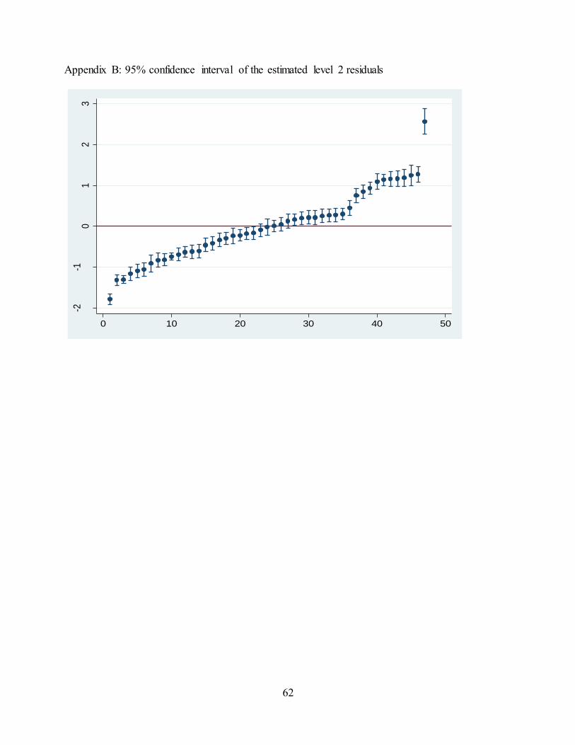
62

Appendix B: 95% confidence interval of the estimated level 2 residuals

-2-1

01

23

0 10 20 30 40 50

63

References

Bord, R. J., & O'Connor, R. E. (1997). The gender gap in environmental attitudes: the case of

perceived vulnerability to risk. Social science quarterly, 830-840.

Brechin, S. R. (1999). Objective problems, subjective values, and global environmentalism:

Evaluating the postmaterialist argument and challenging a new explanation. Social Science

Quarterly, 793-809.

Brechin, S. R., & Kempton, W. (1994). Global environmentalism: A challenge to the

postmaterialism thesis? Social Science Quarterly, 75, 245-269.

Cameron, T. A., & Englin, J. (1997). Respondent experience and contingent valuation of

environmental goods. Journal of Environmental Economics and management, 33(3), 296-

313.

Diekmann, A., & Franzen, A. (1999). The wealth of nations and environmental concern.

Environment and behavior, 31, 540-549.

Dietz, T., Stern, P. C., & Guagnano, G. A. (1998). Social structural and social psychological bases

of environmental concern. Environment and Behavior, 30, 450-471.

Dorsch, M. T. (2014). Economic Development and Determinants of Environmental Concern.

Social Science Quarterly, 95, 960-977.

Doulton, H., & Brown, K. (2009). Ten years to prevent catastrophe?: Discourses of climate change

and international development in the UK press. Global Environmental Change, 19, 191-

202.

64

Dunlap, R. E., Gallup Jr, G. H., & Gallup, A. M. (1993). Of global concern: Results of the health

of the planet survey. Environment: Science and Policy for Sustainable Development,

35(9), 7-39.

Dunlap, R. E., & Mertig, A. G. (1991). The evolution of the US environmental movement from

1970 to 1990: An overview. Society & Natural Resources, 4(3), 209-218.

Dunlap, R. E., & Mertig, A. G. (1997). Global environmental concern: An anomaly for

postmaterialism. Social Science Quarterly, 78, 24-29.

Dunlap, R. E., & York, R. (2008). The globalization of environmental concern and the limits of

the postmaterialist values explanation: Evidence from four multinational surveys. The

Sociological Quarterly, 49, 529-563.

Fairbrother, M. (2012). Rich people, poor people, and environmental concern: Evidence across

nations and time. European sociological review, jcs068.

Franzen, A. (2003). Environmental attitudes in international comparison: An analysis of the ISSP

surveys 1993 and 2000. Social science quarterly, 84(2), 297-308.

Franzen, A., & Meyer, R. (2010). Environmental attitudes in cross-national perspective: A

multilevel analysis of the ISSP 1993 and 2000. European Sociological Review, 26, 219-

234.

Franzen, A., & Vogl, D. (2013). Two decades of measuring environmental attitudes: A

comparative analysis of 33 countries. Global Environmental Change, 23, 1001-1008.

Gelissen, J. (2007). Explaining Popular Support for Environmental Protection A Multilevel

Analysis of 50 Nations. Environment and Behavior, 39, 392-415.

65

Givens, J. E., & Jorgenson, A. K. (2011). The effects of affluence, economic development, and

environmental degradation on environmental concern: a multilevel analysis. Organization

& Environment, 24, 74-91.

Gökşen, F., Adaman, F., & Ünal Zenginobuz, E. (2002). On environmental concern, willingness to

pay, and postmaterialist values evidence from Istanbul. Environment and Behavior, 34,

616-633.

Gupta, A. K., Tesluk, P. E., & Taylor, M. S. (2007). Innovation at and across multiple levels of

analysis. Organization Science, 18(6), 885-897.

Hox, J. J., Moerbeek, M., & van de Schoot, R. (2010). Multilevel analysis: Techniques and

applications. Routledge.

Hunter, L. M., Hatch, A., & Johnson, A. (2004). Cross-national gender variation in environmental

behaviors. Social Science Quarterly, 85, 677-694.

Inglehart, R. (1990). Culture shift in advanced industrial society. Princeton, NJ: Princeton

University Press.

Inglehart, R. (1995). Public support for environmental protection: Objective problems and

subjective values in 43 societies. PS: Political Science & Politics, 28, 57-72.

Inglehart, R. (1997). Modernization and postmodernization. Cultural, political and economic

change in 43 societies. Princeton: Princeton University Press.

Israel, D & Levinson, A. (2004). Willingness to pay for environmental quality: testable empirical

implications of the growth and environmental literature. Contributions to Economic

Analysis and Policy 3 (1) (2).

66

Jorgenson, A. K., & Givens, J. E. (2013). Economic Globalization and Environmental Concern: A

Multilevel Analysis of Individuals within 37 Nations. Environment and Behavior,

0013916513479796.

Kemmelmeier, M., Krol, G., & Kim, Y. H. (2002). Values, economics, and proenvironmental

attitudes in 22 societies. Cross-Cultural Research, 36, 256-285.

Kidd, Q., & Lee, A. R. (1997). Postmaterialist values and the environment: A critique and

reappraisal. Social Science Quarterly, 1-15.

Knight, K. W., & Messer, B. L. (2012). Environmental Concern in Cross‐National Perspective:

The Effects of Affluence, Environmental Degradation, and World Society. Social Science

Quarterly, 93, 521-537.

Laroche, M., Bergeron, J., & Barbaro-Forleo, G. (2001). Targeting consumers who are willing to

pay more for environmentally friendly products. Journal of consumer marketing, 18, 503-

520.

Lo, A. Y., & Chow, A. T. (2015). The relationship between climate change concern and national

wealth. Climatic Change, 1-14.

Marquart-Pyatt, S. T. (2012). Contextual influences on environmental concerns cross-nationally:

A multilevel investigation. Social science research, 41, 1085-1099.

McCright, A. M. (2010). The effects of gender on climate change knowledge and concern in the

American public. Population and Environment, 32(1), 66-87.

67

Meyer, R., & Liebe, U. (2010). Are the affluent prepared to pay for the planet? Explaining

willingness to pay for public and quasi-private environmental goods in Switzerland.

Population and environment, 32, 42-65.

Nawrotzki, R. J. (2012). The politics of environmental concern: a cross-national analysis.

Organization & Environment, 1086026612456535.

Olli, E., Grendstad, G., & Wollebaek, D. (2001). Correlates of environmental behaviors bringing

back social context. Environment and behavior, 33(2), 181-208.

Paavola, J. (2007). Institutions and environmental governance: a reconceptualization. Ecological

economics, 63(1), 93-103.

Running, K. (2013). World Citizenship and Concern for Global Warming: Building the Case for a

Strong International Civil Society. Social forces, sot077.

Sampei, Y., & Aoyagi-Usui, M. (2009). Mass-media coverage, its influence on public awareness

of climate-change issues, and implications for Japan’s national campaign to reduce

greenhouse gas emissions. Global Environmental Change, 19, 203-212.

Sandvik, H. (2008). Public concern over global warming correlates negatively with national

wealth. Climatic Change, 90(3), 333-341.

Schultz, P. W., Zelezny, L., & Dalrymple, N. J. (2000). A multinational perspective on the relation

between Judeo-Christian religious beliefs and attitudes of environmental concern.

Environment and Behavior, 32(4), 576-591.

Scott, D., & Willits, F. K. (1994). Environmental Attitudes and Behavior A Pennsylvania Survey.

Environment and behavior, 26, 239-260.Sulemana, I. (2016). Are Happier People More

68

Willing to Make Income Sacrifices to Protect the Environment?. Social Indicators

Research, 127(1), 447-467.

Sulemana, I., James, H. S., & Valdivia, C. B. (2016a). Perceived socioeconomic status as a

predictor of environmental concern in African and developed countries. Journal of

Environmental Psychology, 46, 83-95.

Sulemana, I., McCann, L., & James Jr, H. S. (2016b). Perceived environmental quality and

subjective well-being: are African countries different from developed countries?

International Journal of Happiness and Development, 3(1), 64-87.

Swallow, S. K., Weaver, T., Opaluch, J. J., & Michelman, T. S. (1994). Heterogeneous

preferences and aggregation in environmental policy analysis: a landfill siting case.

American Journal of Agricultural Economics, 76(3), 431-443.

Tesh, S. N. (1993). Environmentalism, pre-environmentalism, and public policy. Policy sciences,

26(1), 1-20.

Thompson, G. D. (1998). Consumer demand for organic foods: what we know and what we need

to know. American Journal of Agricultural Economics, 80(5), 1113-1118.

Torgler, B., & Garcia-Valiñas, M. A. (2007). The determinants of individuals' attitudes towards

preventing environmental damage. Ecological economics, 63, 536-55.

Torgler, B., Garcia-Valiñas, M. A., & Macintyre, A. (2008). Differences in preferences towards

the environment: the Impact of a gender, age and parental effect. Working paper.

Veisten, K.,Hoen, H.F.,Navrud, S & Strand, J., (2004). Scope insensitivity in contingent valuation

of complex environmental amenities. Journal of Environmental Management 73, 317–331.

69

Yuchtman-Yaar, E., & Alkalay, Y. (2007). Religious zones, economic development and modern

value orientations: Individual versus contextual effects. Social Science Research, 36(2),

789-807.

Zelezny, L. C., & Yelverton, J. A. (2000). Feminine identity, collectivism, and environmental

attitudes and behaviors. In meeting of the Western Psychological Association, Portland,

OR.

70

71

72

Chapter 2. On the relationship between CO2 emissions and economic

growth: Evidence from panel smooth transition regression16

16 Revised and resubmitted in Environment, Development and Sustainability, currently under review.

73

2.1. Introduction

Ever since the seminal work of Grossman and Krueger (1991) that led to finding an inverted U-

shape relation between environmental degradation and economic growth, a large and still-growing

body of literature has continued to identify aspects of the relationship between various measures of

environmental quality and economic growth. The presumptive assumption held by these studies is

that, environmental quality deteriorates in the early stages of economic growth and then improves

in the later stages once economic growth has reached a certain threshold. This phenomenon has been

termed “Environmental Kuznets Curve” (EKC) because of its resemblance to the relationship

between inequality and income levels observed by Kuznets (1955). The EKC has gained tremendous

enthusiasm both from the theoretical framework and environmental policies17. From policy-mak ing

perspectives, the EKC constitutes the cornerstone for establishing a strategic plan to achieve

sustainable economic growth.

From a theoretical standpoint, a number of papers have posited explanations for the observed pattern

between emissions and economic growth. At the core of this body of theoretical literature is the

study by Arrow et al. (1995) which postulates that environmental quality generally worsens during

the initial phases of economic growth but when societies have achieved relatively more advanced

stages of economic growth, they tend to give greater attention to environmental quality through

either market mechanisms or regulatory policies. A second type of explanation is contained in

studies that decompose the change of pollution emissions into scale, composition and technique

effects (Grossman and Krueger, 1995; Antweiler et al, 2001 and Brock and Taylor, 2005). These

authors offer the explanation that a scale effect arises from an expansion of economic activity, but

17 Stern (2004) and Dinda (2004) provide a comprehensive review of earlier studies on the EKC framework. A more recent studies on the EKC literature is found in Kijima et al. (2010).

74

when economic activity shifts from energy-intensive industries to cleaner ones, emissions fall

through the composition effect, and that because of this investments in environmentally-friend ly

technology become more effective thus leading to sustainable development. A related explanation

offered by Dinda (2004) describes the EKC as a natural progression of economic growth, from a

clean agrarian economy to a polluting industrial to a cleaner service economy.

Thus, the main goal of this chapter is to investigate the nature of the relationship between CO2

emissions and economic growth of 96 countries over the period 1984-2013. In doing so, the study

contributes to the existing literature by, first, applying the Panel Smooth Transition Regression

(PSTR) model of González et al. (2005); and, second, by incorporating energy consumption,

industrialization, urbanization, trade openness, capital expenditures and quality of institutions in the

model besides CO2 emissions and economic growth to solve the omitted variable bias issue suffered

by most previous studies. To the best of our knowledge, this is the first study that account for the

quality of institutions into the relationship between CO2 emissions and economic growth. Finally,

we also dealt with potential endogeneity of regressors through Instrumental Variable estimation.

The study unveils the existence of a non-linear relation between CO2 emissions and economic

growth rather than an inverted U-shaped relation. Interestingly, we also find evidence suggest ing

that quality of institutions matters to the relationship between CO2 emissions and economic growth;

better quality of institutions enhances environmental quality.

The remainder of the chapter is organized as follows. The next section briefly reviews the literature

on CO2 emissions and economic growth relation. Section 2.3. introduces the PSTR model and

testing procedure. Section 2.4. describes data sources and variable definitions. Section 2.5. presents

the empirical results and discusses their implications. Finally, the last section will conclude.

75

2.2. Brief literature review

Despite the numerous attempts that contributed to the discussion and to deepen our understand ing

of the nature of the relationship between different types of emissions and economic growth, there

still is no consensus among scholars as to why and how exactly the EKC relationship emerges for

certain environmental indicators but not for others18. Studies have found different results for the

same pollutant by using different time frame and estimation techniques (Ekins, 1997). For instance,

Schmalensee et al. (1998) use a piecewise linear function to investigate the relationship between

CO2 emissions and economic growth. By adopting the piecewise linear function, the authors find

evidence of an EKC for CO2 emissions. To add to the list, Galeotti et al. (2006) employ a more

flexible functional form, the Weibull function to validate the EKC hypothesis. They find evidence

of an inverted U-pattern for the group of OECD countries but not so for non-OECD countries. Luo

et al. (2017) investigate whether the EKC holds in a group of G20 countries. By accounting for

trade openness, the ratio industry value-added to GDP and population density as additional control

variables, they find evidence pointing toward the EKC hypothesis for the G20 members. Martino

and Van (2016) employ an instrumental semiparametric panel model and apply it to data consisting

of 106 countries over the 1970-2010 period. They find no evidence supporting the EKC, even for

the OECD countries. Azomahou et al. (2006) depart from the parametric functions and adopt a non-

parametric approach to investigate the relationship between CO2 emissions and economic growth

18 Empirical literature has documented that EKC hold for local pollutants such as sulfur oxides (SOx), nitrogen oxides (NOx), carbon monoxide (CO) and suspended particulate matter (SPM) (Selden and Song, 1994; Stern and Common, 2001; Harbaugh et al, 2002; Brock and Taylor, 2010; Miah et al, 2010; Liddle and Messinis, 2015; Georgiev and Mihaylov, 2015; Wang et al, 2016; Fujii, and Managi, 2016). In the case of global emissions, however, the empirical findings are still far from convergent and it is not difficult to find conflicting results. For instance, Ahmed and Long, (2012); Kaika and Zervas, (2013); Apergis and Ozturk, (2015) and Balaguer and Cantavella, (2016) have found evidence pointing towards the inverted U-shape while Du et al, (2012); Al-Mulali et al, (2015); Yang et al. (2015) and Baek, (2015) have reported environmental quality declines with increasing income.

76

of a panel of 100 countries over the period 1960-1996. Their finding indicates that the relationship

between the two variables is upward sloping. Using the Common Correlated Effects (CCE)

estimation procedure by Pesaran (2006), Apergis et al. (2017) assess the validity of the EKC

hypothesis across 48 US states. The findings suggest that the EKC hypothesis holds in only 10

states. Narayan and Narayan (2010) examine the EKC for 43 developing countries using the panel

cointegration and the panel long-run estimation techniques. Their findings support the inverted U-

shaped curve only for the group of Middle East and South Asian countries.

More recently, works such as Stern et al. (1996) and Stern (2015), have raised concerns over the

functional forms and estimation methods used to investigate the relationship between different

indicators of environmental quality and economic growth. They claim that previous studies have

arbitrarily modeled and estimated a quadratic polynomial framework to capture the non-linear ity

between emissions and economic growth. One of the drawbacks mentioned of using the quadratic

polynomial is that it ignores the presence of heterogeneity across countries. To remedy econometric

issues in estimation due to the aribitrary choice of functional forms and to deal with heterogeneity

issue, González et al. (2005) propose the Panel Smooth Transition Regression (PSTR) as estimation

technique to alleviate these issues. The PSTR addresses the problems of heterogeneity and time

instability in a non-linear setting. Furthermore, the PSTR presents significant advantages over the

traditional quadratic polynomial model19. Firstly, the PSTR permits a continuum in the country-

specific correlation with respect to the threshold variable. Secondly, it allows the emissions-

economic growth relation coefficient to vary between countries and over time. Lately, some studies

have applied the PSTR to investigate the non-linearities between macroeconomic variables. See for

19Aslanidis and Xepapadeas (2006) show the quadratic or cubic polynomial model used in the literature is a specific case of the more general PSTR.

77

instance, Bessec and Fouquau (2008) on the relationship between electricity demand and

temperature; Chiu (2012) on deforestation and per capita income; Duarte et al. (2013) on per capita

water use and per capita income; Seleteng et al, (2013) and Thanh (2015) on inflation and economic

growth.

In the present chapter, we have adopted the PSTR by González et al. (2005) to study the complex

links between CO2 emissions and economic growth.

2.3. Econometric methodology

2.3.1. PSTR model specification

To investigate the potential non-linear relationship between per capita CO2 emissions and economic

growth, we apply the more flexible econometric technique, the PSTR developed by González et al.

(2005). The PSTR is a suitable approach to account for cross-country heterogeneity and time

variability of the slope coefficients. Furthermore, it accommodates for the presence of exogenous

variables with constant coefficients. The PSTR can be viewed as a generalization of the Panel

Threshold Regression (PTR) model proposed by Hansen (1999). Contrary to the PTR model that

imposes a sharp shift when transitioning from one regime to another, the PSTR model allows the

regression coefficients to switch gradually from one regime to the next.

Therefore, the equation used to estimate the non-linear relationship between per capita CO2

emissions and economic growth is a two extreme regimes PSTR model with single transit ion

function and some control variables as stated below:

𝑙𝑛𝐶𝑂2𝑖𝑡 = 𝜇𝑖 + 𝛽0𝑙𝑛𝐺𝐷𝑃𝑖𝑡 + 𝛽1𝑙𝑛𝐺𝐷𝑃𝑖𝑡𝑔(𝑙𝑛𝐺𝐷𝑃𝑖𝑡−1; 𝛾, 𝑐) + 𝛼0′ 𝑍𝑖𝑡+𝜖𝑖𝑡 (1)

78

where 𝑖 = 1,2, … , 𝑁 and 𝑡 = 1,2, … , 𝑇 denote the cross-section and time dimensions, respectively.

The dependent variable 𝑙𝑛𝐶𝑂2𝑖𝑡 is the log value of per capita CO2 emissions, 𝜇𝑖 represents the

country-specific effects and 𝑙𝑛𝐺𝐷𝑃𝑖𝑡 refers to the log value of real gross domestic product GDP per

capita; 𝑍𝑖𝑡 is a 𝑘-dimensional vector of a set of time-invariant exogenous variables which includes :

energy consumption per capita; industrialization level, which is proxied with the ratio of industry

value added in GDP; urbanization level, measured by the fraction of the population living in urban

areas; the ratio of gross fixed capital formation to GDP; and import and export of merchandise as

percentages of GDP. Institutional quality variables were also controlled for to gauge to what extent

the quality of institutions matter for environmental pollution. The transition function

𝑔(𝑙𝑛𝐺𝐷𝑃𝑖𝑡−1,𝛾, 𝑐) is a continuous function normalized and bounded between 0 and 1 of the

observable variable 𝑙𝑛𝐺𝐷𝑃𝑖𝑡−1. As noted by van Dijk et al. (2002), the threshold variable can be an

exogenous variable or a combination of the lagged endogenous one. To estimate the effect of GDP

per capita on per capita CO2 emissions, we consider in this study the lagged level of the log of the

real GDP per capita as a threshold variable. The slope parameter 𝛾 denotes the smoothness of the

transition function from one regime to another, 𝑐 is the threshold or location parameter, and 𝜖𝑖𝑡 is

the error term. It is worth mentioning that 𝛾 and 𝑐 are endogenously determined.

Following the methodology proposed by Granger and Teräsvirta (1993), Teräsvirta (1994),

Jansen and Teräsvirta (1996), and the extension to panel data by González et al. (2005), the logist ic

transition function is formulated as follows:

𝑔(𝑙𝑛𝐺𝐷𝑃𝑖𝑡−1;𝛾, 𝑐) = (1 + 𝑒𝑥𝑝(−𝛾 ∏ (𝑙𝑛𝐺𝐷𝑃𝑖𝑡−1 − 𝑐𝑗)𝑚𝑗=1 ))

−1

, 𝛾 > 0, 𝑐1 ≤ 𝑐2 ≤ ⋯ ≤ 𝑐𝑚 (2)

where 𝑐 = (𝑐1, … , 𝑐𝑚)′ denotes an 𝑚-dimensional vector of location parameters. Restrictions on 𝛾 >

0 and 𝑐1 ≤ 𝑐2 ≤ ⋯ ≤ 𝑐𝑚 are imposed for identification. González et al. (2005) indicate that in

79

empirical exercise, it is sufficient to consider 𝑚 = 1 or 𝑚 = 2 to capture the non-linearities due to

regime switching. The case 𝑚=1 refers to a logistic PSTR model while the case 𝑚=2 corresponds to

a logistic quadratic PSTR specification (Bereau et al. 2010). When 𝛾 → ∞, the transition function

𝑔(𝑙𝑛𝐺𝐷𝑃𝑖𝑡−1;𝛾, 𝑐) becomes an indicator function and the PSTR turns into a PTR model (Hansen,

1999). However, when 𝛾 → 0, the transition function 𝑔(𝑙𝑛𝐺𝐷𝑃𝑖𝑡−1;𝛾, 𝑐) becomes constant and the

model collapses into a standard linear panel regression model with fixed effects.

Hence, the PSTR model has many advantages over the widely applied quadratic polynomial model.

First and foremost, the PSTR allows the parameters to vary across countries and over time. Second,

parameters are allowed to change smoothly with the threshold variable 𝑙𝑛𝐺𝐷𝑃𝑖𝑡−1. Another

advantage of the PSTR is that the value of the elasticities for a given country and at a given date can

be different from the estimated parameters for the extreme regimes. Thus, the impact of the real

GDP per capita on per capita CO2 emissions is given by:

𝜕𝑙𝑛𝐶𝑂2𝑖𝑡

𝜕𝑙𝑛𝐺𝐷𝑃𝑖𝑡= 𝛽0 + 𝛽1 𝑔(𝑙𝑛𝐺𝐷𝑃𝑖𝑡−1,𝛾, 𝑐) (3)

Given the properties of the transition function, the parameter 𝛽0 corresponds to the elasticity only if

the transition function 𝑔(𝑙𝑛𝐺𝐷𝑃𝑖𝑡−1, 𝛾, 𝑐) tends to 0. The sum of the parameters 𝛽0 and β1 corresponds

to the elasticity only if the transition function 𝑔(𝑙𝑛𝐺𝐷𝑃𝑖𝑡−1,𝛾, 𝑐) tends to 1. At any point between

these two extremes, the elasticity is defined as a weighted average of the parameters 𝛽0 and 𝛽1. As

a consequence, it is possible only to interpret the signs of the parameters rather than their

magnitudes.

80

2.3.2. Model specification and testing procedure

González et al. (2005) also propose a test for linearity against the PSTR model as well as a test of

no remaining linearity. As outlined in their paper, the procedure for testing the null hypothesis of

linearity consists of testing the null hypothesis: 𝐻0: 𝛾 = 0 or 𝐻0: 𝛽0 = 𝛽1 . In both cases, the test is

non-standard since, under the null hypothesis, the PSTR model contains unidentified nuisance

parameters. That is, classical test is not valid. A viable solution to this issue consists of replacing

the transition function 𝑔(𝑙𝑛𝐺𝐷𝑃𝑖𝑡−1,𝛾, 𝑐) by its first-order Taylor expansion around the null

hypothesis: 𝐻0: 𝛾 = 0 and by testing an equivalent hypothesis in an auxiliary regression model

that takes the following form:

𝑙𝑛𝐶𝑂2𝑖𝑡 = 𝜇𝑖 + 𝛽0∗𝐿𝑛𝐺𝐷𝑃𝑖𝑡 + 𝛽1

∗𝑙𝑛𝐺𝐷𝑃𝑖𝑡𝑙𝑛𝐺𝐷𝑃𝑖𝑡−1 + ⋯ + 𝛽𝑚∗ 𝑙𝑛𝐺𝐷𝑃𝑖𝑡𝑙𝑛𝐺𝐷𝑃𝑖𝑡−1

𝑚 + 𝜖𝑖𝑡∗ (4)

the parameters 𝛽0∗,… , 𝛽𝑚

∗ are multiples of 𝛾 and 𝜖𝑖𝑡∗ = 𝜖𝑖𝑡 + 𝑅𝑚𝛽1

∗𝑙𝑛𝐺𝐷𝑃𝑖𝑡, where 𝑅𝑚 is the remainder

of the Taylor expansion.Therefore, testing 𝐻0: 𝛾 = 0 in Eq. (1) is equivalent to testing the null

hypothesis: 𝐻0: 𝛽1∗ = ⋯ = 𝛽𝑚

∗ = 0 in Eq. (4). Following Colletaz and Hurlin (2006), three type of

tests have been performed to assess the linearity. The Wald test:

𝐿𝑀𝑤 = 𝑁𝑇(𝑆𝑆𝑅0 − 𝑆𝑆𝑅1)/𝑆𝑆𝑅0 (5)

where 𝑆𝑆𝑅0 is the panel sum of the squared residuals under the null hypothesis (linear model with

individual effects) and 𝑆𝑆𝑅1 is the panel sum of the squared residuals under the alternat ive

hypothesis (PSTR model with two regimes). Likewise, the Fisher test is defined as follows:

81

𝐿𝑀𝑓 = [𝑁𝑇(𝑆𝑆𝑅0 − 𝑆𝑆𝑅1)/𝑚𝐾]/[𝑆𝑆𝑅0 /(𝑇𝑁 − 𝑁 − 𝑚(𝐾 + 1))] (6)

where 𝐾 is the number of explanatory variables and 𝑚 the number of regimes. And finally, the

pseudo-likelihood ratio test is given by:

𝐿𝑅 = −2[𝑙𝑜𝑔(𝑆𝑆𝑅1) − 𝑙𝑜𝑔 (𝑆𝑆𝑅0)] (7)

Under the null hypothesis, the Wald and likelihood ratio statistics have an asymptotic 𝜒2(𝑚𝑘)

distribution while the Fisher statistic is approximated to have the distribution of 𝐹(𝑚𝐾, 𝑇𝑁 −

𝑁– 𝑚𝐾).

If the linearity hypothesis is rejected, then the next step consists of testing for no remaining linearity.

In other words, we test whether there is one transition function or if, on the other hand, there are at

least two transition functions. This is done by testing the following hypothesis: 𝐻0:𝑟 = 𝑟∗ against

𝐻1: 𝑟 = 𝑟∗ + 1. If 𝐻0 is not rejected, the procedure stops. Otherwise, the null hypothesis : 𝐻0:𝑟 = 𝑟∗ +

1 is tested against 𝐻1: 𝑟 = 𝑟∗ + 2. Then the testing sequence continues until the first acceptance of

the null hypothesis of no remaining linearity. It is important to bear in mind that the estimation of

the PSTR model is conducted by first eliminating the individual effects 𝜇𝑖.Then a grid search is

performed to obtain initial values for the slopes and the location parameters by applying Non-Linear

Least Squares (NLS) to the transformed data. This estimation technique is equivalent to the

maximum likelihood estimation since the error term 𝜖𝑖𝑡 follows a normal distribution.

2.3.3. PSTR estimates and endogeneity

The literature has suggested that first difference transformations and non-linear modeling strategies

mitigate endogeneity issues (Omay and Kan, 2010; Lopez Villavicencio and Mignon (2011).

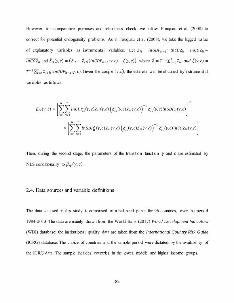
82

However, for comparative purposes and robustness check, we follow Fouquau et al. (2008) to

correct for potential endogeneity problems. As in Fouquau et al. (2008), we take the lagged value

of explanatory variables as instrumental variables. Let 𝑍𝑖𝑡 = 𝑙𝑛𝐺𝐷𝑃𝑖𝑡−1; 𝑙𝑛𝐶𝑂2̃𝑖𝑡 = 𝑙𝑛𝐶𝑂2𝑖𝑡 −

𝑙𝑛𝐶𝑂2̅̅ ̅̅ ̅̅ ̅̅𝑖𝑡 and �̃�𝑖𝑡(𝛾, 𝑐) = (𝑍𝑖𝑡 − 𝑍̅, 𝑔(𝑙𝑛𝐺𝐷𝑃𝑖𝑡−1; 𝛾, 𝑐) − 휁̅(𝛾, 𝑐)), where 𝑍̅ = 𝑇−1 ∑ 𝑍𝑖𝑡

𝑇𝑡=1 and 휁̅(𝛾, 𝑐) =

𝑇−1 ∑ 𝑍𝑖𝑡 𝑔(𝑙𝑛𝐺𝐷𝑃𝑖𝑡−1;𝛾, 𝑐)𝑇𝑡=1 . Given the couple (𝛾, 𝑐), the estimate will be obtained by instrumenta l

variables as follows:

�̂�𝐼𝑉(𝛾, 𝑐) = [∑ ∑ 𝑙𝑛𝐺𝐷�̃�𝑖𝑡′ (𝛾, 𝑐)�̃�𝑖𝑡(𝛾, 𝑐) (�̃�𝑖𝑡

′ (𝛾,𝑐)�̃�𝑖𝑡(𝛾, 𝑐))−1

�̃�𝑖𝑡′ (𝛾, 𝑐)𝑙𝑛𝐺𝐷�̃�𝑖𝑡(𝛾, 𝑐)

𝑇

𝑡=1

𝑁

𝑖=1

]

−1

× [∑ ∑𝑙𝑛𝐺𝐷�̃�𝑖𝑡′ (𝛾, 𝑐)�̃�𝑖𝑡(𝛾, 𝑐) (�̃�𝑖𝑡

′ (𝛾, 𝑐)�̃�𝑖𝑡(𝛾, 𝑐))−1

�̃�𝑖𝑡′ (𝛾, 𝑐)𝑙𝑛𝐶𝑂2̃𝑖𝑡(𝛾,𝑐)

𝑇

𝑡=1

𝑁

𝑖=1

]

Then, during the second stage, the parameters of the transition function 𝛾 and 𝑐 are estimated by

NLS conditionally to �̂�𝐼𝑉(𝛾, 𝑐).

2.4. Data sources and variable definitions

The data set used in this study is comprised of a balanced panel for 96 countries, over the period

1984-2013. The data are mainly drawn from the World Bank (2017) World Development Indicators

(WDI) database; the institutional quality data are taken from the International Country Risk Guide

(ICRG) database. The choice of countries and the sample period were dictated by the availability of

the ICRG data. The sample includes countries in the lower, middle and higher income groups.

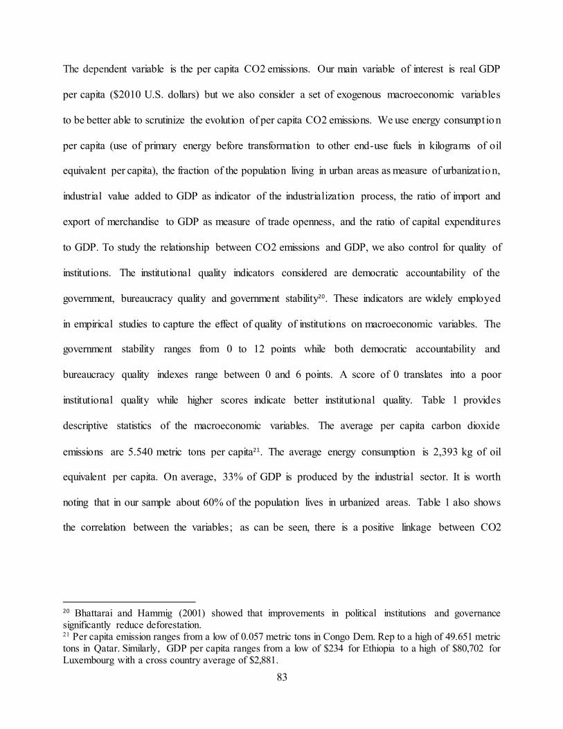
83

The dependent variable is the per capita CO2 emissions. Our main variable of interest is real GDP

per capita ($2010 U.S. dollars) but we also consider a set of exogenous macroeconomic variables

to be better able to scrutinize the evolution of per capita CO2 emissions. We use energy consumption

per capita (use of primary energy before transformation to other end-use fuels in kilograms of oil

equivalent per capita), the fraction of the population living in urban areas as measure of urbanizat ion,

industrial value added to GDP as indicator of the industrialization process, the ratio of import and

export of merchandise to GDP as measure of trade openness, and the ratio of capital expenditures

to GDP. To study the relationship between CO2 emissions and GDP, we also control for quality of

institutions. The institutional quality indicators considered are democratic accountability of the

government, bureaucracy quality and government stability20. These indicators are widely employed

in empirical studies to capture the effect of quality of institutions on macroeconomic variables. The

government stability ranges from 0 to 12 points while both democratic accountability and

bureaucracy quality indexes range between 0 and 6 points. A score of 0 translates into a poor

institutional quality while higher scores indicate better institutional quality. Table 1 provides

descriptive statistics of the macroeconomic variables. The average per capita carbon dioxide

emissions are 5.540 metric tons per capita21. The average energy consumption is 2,393 kg of oil

equivalent per capita. On average, 33% of GDP is produced by the industrial sector. It is worth

noting that in our sample about 60% of the population lives in urbanized areas. Table 1 also shows

the correlation between the variables; as can be seen, there is a positive linkage between CO2

20 Bhattarai and Hammig (2001) showed that improvements in political institutions and governance significantly reduce deforestation. 21 Per capita emission ranges from a low of 0.057 metric tons in Congo Dem. Rep to a high of 49.651 metric tons in Qatar. Similarly, GDP per capita ranges from a low of $234 for Ethiopia to a high of $80,702 for Luxembourg with a cross country average of $2,881.

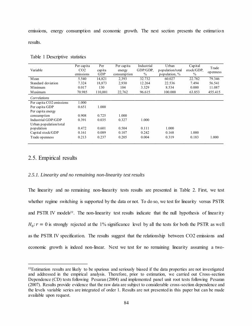
84

emissions, energy consumption and economic growth. The next section presents the estimation

results.

Table 1 Descriptive statistics

Variable Per capita

CO2 emissions

Per capita GDP

Per capita energy

consumption

Industrial GDP/GDP,

%

Urban population/total population, %

Capital stock/GDP,

%

Trade openness

Mean 5.540 14,821 2,393 32.732 60.027 22.782 79.346 Standard deviation 7.324 18,873 2,930 12.264 22.536 7.494 56.541 Minimum 0.017 130 104 3.329 8.534 0.000 11.087 Maximum 70.985 110,001 22,762 96.615 100.000 63.853 455.415 Correlations Per capita CO2 emissions 1.000 Per capita GDP 0.651 1.000 Per capita energy consumption 0.908 0.725 1.000 Industrial GDP/GDP 0.391 0.035 0.327 1.000 Urban population/total population 0.472 0.601 0.504 0.111 1.000 Capital stock/GDP 0.161 0.089 0.107 0.242 0.168 1.000 Trade openness 0.213 0.237 0.205 0.004 0.319 0.183 1.000

2.5. Empirical results

2.5.1. Linearity and no remaining non-linearity test results

The linearity and no remaining non-linearity tests results are presented in Table 2. First, we test

whether regime switching is supported by the data or not. To do so, we test for linearity versus PSTR

and PSTR IV models22. The non-linearity test results indicate that the null hypothesis of linear ity

𝐻0: 𝑟 = 0 is strongly rejected at the 1% significance level by all the tests for both the PSTR as well

as the PSTR IV specification. The results suggest that the relationship between CO2 emissions and

economic growth is indeed non-linear. Next we test for no remaining linearity assuming a two-

22Estimation results are likely to be spurious and seriously biased if the data properties are not investigated and addressed in the empirical analysis. Therefore, prior to estimation, we carried out Cross-section Dependence (CD) tests following Pesaran (2004) and implemented panel unit root tests following Pesaran (2007). Results provide evidence that the raw data are subject to considerable cross-section dependence and the levels variable series are integrated of order 1. Results are not presented in this paper but can be made available upon request.

85

regime model. The results clearly indicate that the null hypothesis 𝐻0: 𝑟 = 1 cannot be rejected at

the 5% significance level, which implies that the model has one threshold or two regimes. As a

result, one threshold was sufficient to capture the non-linearity in the relationships between CO2

emissions and economic growth. Consequently, we choose to estimate models with one transit ion

function and one location parameter.

Table 2 Linearity and no remaining non-linearity tests of the PSTR and PSTR IV models Model PSTR PSTR IV

H0: r=0 vs H1: r=1 Statistic p-value Statistic p-value Lagrange multiplier — Wald 469.191*** 0.000 464.735*** 0.000 Lagrange multiplier — Fischer 270.716*** 0.000 267.650*** 0.000 Likelihood ratio 512.145*** 0.000 506.826*** 0.000

H0: r=1 vs H1: r=2

Lagrange multiplier — Wald 254.155 0.063 197.268 0.082 Lagrange multiplier — Fischer 169.365 0.057 204.641 0.076 Likelihood ratio 266.075 0.062 204.349** 0.023

Notes: Under H0, the Wald and Likelihood ratio statistics have asymptotic χ2(mK) distribution, whereas the Fisher has an asymptotic F(mK,

TN−N−m(K+1)) distribution. Moreover, r is the number of transition function. r=0, (1 regime no transition function), r=1, (2 regimes 1 transition function), r=2, (3 regimes 2 transitions). (***), (**) denote significance at 1% and 5%, respectively.

2.5.2. PSTR estimation results

The parameter estimates of the PSTR models are reported in column [1] through column [12] of

Table 3. The table also presents the standard errors corrected for heteroskedasticity. The results of

the model 1 consider only GDP per capita and one transition variable as regressors, while model 2

onwards control for some additional variables that might have an impact on CO2 emissions. It is

worth mentioning that only the signs of the estimated parameters on GDP per capita and GDP as

transition variable can be interpreted; however, both the sign and the magnitude of the control

variables have meaningful interpretations.

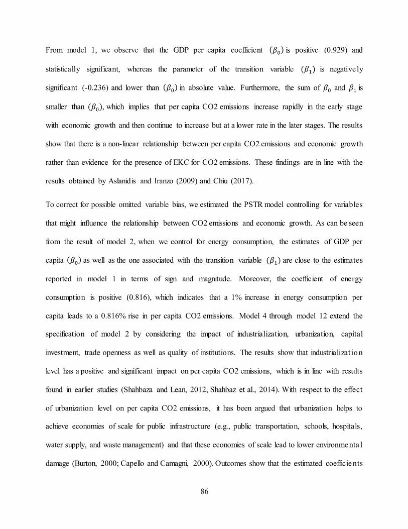
86

From model 1, we observe that the GDP per capita coefficient (𝛽0) is positive (0.929) and

statistically significant, whereas the parameter of the transition variable (𝛽1) is negative ly

significant (-0.236) and lower than (𝛽0) in absolute value. Furthermore, the sum of 𝛽0 and 𝛽1 is

smaller than (𝛽0), which implies that per capita CO2 emissions increase rapidly in the early stage

with economic growth and then continue to increase but at a lower rate in the later stages. The results

show that there is a non-linear relationship between per capita CO2 emissions and economic growth

rather than evidence for the presence of EKC for CO2 emissions. These findings are in line with the

results obtained by Aslanidis and Iranzo (2009) and Chiu (2017).

To correct for possible omitted variable bias, we estimated the PSTR model controlling for variables

that might influence the relationship between CO2 emissions and economic growth. As can be seen

from the result of model 2, when we control for energy consumption, the estimates of GDP per

capita (𝛽0) as well as the one associated with the transition variable (𝛽1) are close to the estimates

reported in model 1 in terms of sign and magnitude. Moreover, the coefficient of energy

consumption is positive (0.816), which indicates that a 1% increase in energy consumption per

capita leads to a 0.816% rise in per capita CO2 emissions. Model 4 through model 12 extend the

specification of model 2 by considering the impact of industrialization, urbanization, capital

investment, trade openness as well as quality of institutions. The results show that industrializat ion

level has a positive and significant impact on per capita CO2 emissions, which is in line with results

found in earlier studies (Shahbaza and Lean, 2012, Shahbaz et al., 2014). With respect to the effect

of urbanization level on per capita CO2 emissions, it has been argued that urbanization helps to

achieve economies of scale for public infrastructure (e.g., public transportation, schools, hospitals,

water supply, and waste management) and that these economies of scale lead to lower environmenta l

damage (Burton, 2000; Capello and Camagni, 2000). Outcomes show that the estimated coefficients

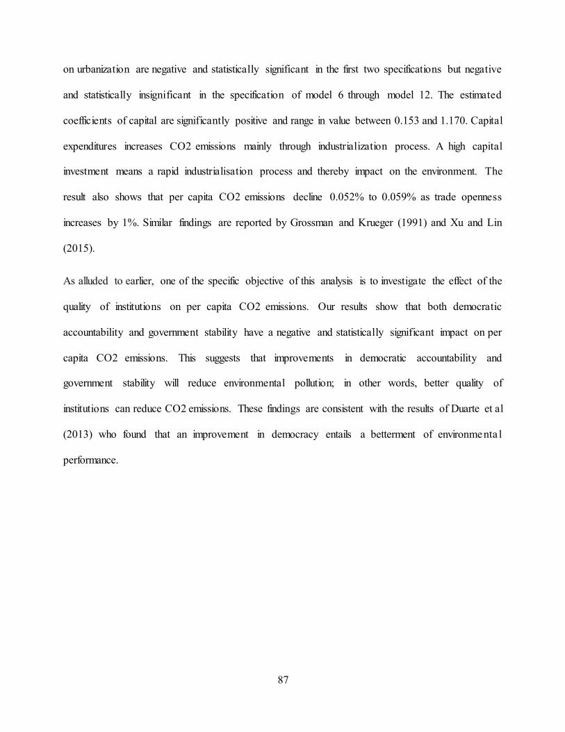
87

on urbanization are negative and statistically significant in the first two specifications but negative

and statistically insignificant in the specification of model 6 through model 12. The estimated

coefficients of capital are significantly positive and range in value between 0.153 and 1.170. Capital

expenditures increases CO2 emissions mainly through industrialization process. A high capital

investment means a rapid industrialisation process and thereby impact on the environment. The

result also shows that per capita CO2 emissions decline 0.052% to 0.059% as trade openness

increases by 1%. Similar findings are reported by Grossman and Krueger (1991) and Xu and Lin

(2015).

As alluded to earlier, one of the specific objective of this analysis is to investigate the effect of the

quality of institutions on per capita CO2 emissions. Our results show that both democratic

accountability and government stability have a negative and statistically significant impact on per

capita CO2 emissions. This suggests that improvements in democratic accountability and

government stability will reduce environmental pollution; in other words, better quality of

institutions can reduce CO2 emissions. These findings are consistent with the results of Duarte et al

(2013) who found that an improvement in democracy entails a betterment of environmenta l

performance.

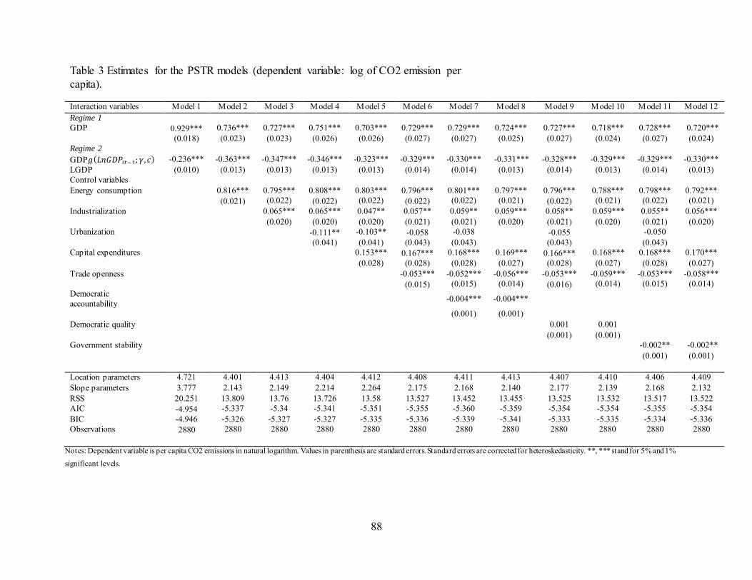
88

Table 3 Estimates for the PSTR models (dependent variable: log of CO2 emission per capita). Interaction variables Model 1 Model 2 Model 3 Model 4 Model 5 Model 6 Model 7 Model 8 Model 9 Model 10 Model 11 Model 12 Regime 1 GDP 0.929*** 0.736*** 0.727*** 0.751*** 0.703*** 0.729*** 0.729*** 0.724*** 0.727*** 0.718*** 0.728*** 0.720***

(0.018) (0.023) (0.023) (0.026) (0.026) (0.027) (0.027) (0.025) (0.027) (0.024) (0.027) (0.024) Regime 2 GDP𝑔(𝐿𝑛𝐺𝐷𝑃𝑖𝑡−1; 𝛾, 𝑐) -0.236*** -0.363*** -0.347*** -0.346*** -0.323*** -0.329*** -0.330*** -0.331*** -0.328*** -0.329*** -0.329*** -0.330*** LGDP (0.010) (0.013) (0.013) (0.013) (0.013) (0.014) (0.014) (0.013) (0.014) (0.013) (0.014) (0.013) Control variables Energy consumption 0.816*** 0.795*** 0.808*** 0.803*** 0.796*** 0.801*** 0.797*** 0.796*** 0.788*** 0.798*** 0.792***

(0.021) (0.022) (0.022) (0.022) (0.022) (0.022) (0.021) (0.022) (0.021) (0.022) (0.021) Industrialization 0.065*** 0.065*** 0.047** 0.057** 0.059** 0.059*** 0.058** 0.059*** 0.055** 0.056***

(0.020) (0.020) (0.020) (0.021) (0.021) (0.020) (0.021) (0.020) (0.021) (0.020) Urbanization -0.111** -0.103** -0.058 -0.038 -0.055 -0.050

(0.041) (0.041) (0.043) (0.043) (0.043) (0.043) Capital expenditures

0.153*** 0.167*** 0.168*** 0.169*** 0.166*** 0.168*** 0.168*** 0.170***

(0.028) (0.028) (0.028) (0.027) (0.028) (0.027) (0.028) (0.027) Trade openness -0.053*** -0.052*** -0.056*** -0.053*** -0.059*** -0.053*** -0.058***

(0.015) (0.015) (0.014) (0.016) (0.014) (0.015) (0.014) Democratic accountability

-0.004*** -0.004***

(0.001) (0.001)

Democratic quality 0.001 0.001

(0.001) (0.001) Government stability -0.002** -0.002**

(0.001) (0.001) Location parameters 4.721 4.401 4.413 4.404 4.412 4.408 4.411 4.413 4.407 4.410 4.406 4.409 Slope parameters 3.777 2.143 2.149 2.214 2.264 2.175 2.168 2.140 2.177 2.139 2.168 2.132 RSS 20.251 13.809 13.76 13.726 13.58 13.527 13.452 13.455 13.525 13.532 13.517 13.522 AIC -4.954 -5.337 -5.34 -5.341 -5.351 -5.355 -5.360 -5.359 -5.354 -5.354 -5.355 -5.354 BIC -4.946 -5.326 -5.327 -5.327 -5.335 -5.336 -5.339 -5.341 -5.333 -5.335 -5.334 -5.336 Observations 2880 2880 2880 2880 2880 2880 2880 2880 2880 2880 2880 2880

Notes: Dependent variable is per capita CO2 emissions in natural logarithm. Values in parenthesis are standard errors. Standard errors are corrected for heteroskedasticity. **, *** stand for 5% and 1% significant levels.

89

To check for the robustness of the results reported earlier, we also correct for possible endogeneity

issues. Table 4 reports the estimation results of PSTR IV. In sum, our estimates reach the same

general conclusion as those reported in Table 3. That is, the estimated coefficients of GDP per capita

in the first regime are greater than the coefficients of GDP per capita as transition variable in

absolute terms after correcting for endogeneity. The results provide evidence of a non-linear

relationship between per capita CO2 emissions and GDP per capita. We observe that the slope

coefficients for energy consumption variables are somewhat close to the estimated coefficients

obtained by PSTR. In most specifications, the parameters of the control variables are comparable to

the parameters reported in Table 3. With respect to the quality of institution variables, we find that

democratic accountability has a negative and statistically significant impact on per capita CO2

emissions. However, the only variable that ceases to be statistically significant after controlling for

endogeneity is government stability.

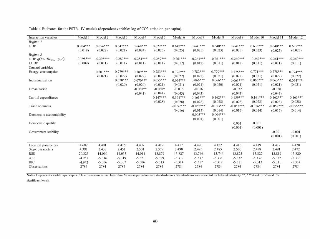
90

Table 4 Estimates for the PSTR- IV models (dependent variable: log of CO2 emission per capita). Interaction variables Model 1 Model 2 Model 3 Model 4 Model 5 Model 6 Model 7 Model 8 Model 9 Model 10 Model 11 Model 12 Regime 1 GDP 0.904*** 0.654*** 0.647*** 0.668*** 0.622*** 0.642*** 0.643*** 0.640*** 0.641*** 0.635*** 0.640*** 0.635***

(0.018) (0.022) (0.021) (0.024) (0.025) (0.025) (0.025) (0.023) (0.025) (0.023) (0.025) (0.023) Regime 2 GDP 𝑔(𝐿𝑛𝐺𝐷𝑃𝑖𝑡 −1; 𝛾, 𝑐) -0.198*** -0.295*** -0.280*** -0.281*** -0.259*** -0.261*** -0.261*** -0.261*** -0.260*** -0.259*** -0.261*** -0.260*** LGDP (0.009) (0.011) (0.011) (0.011) (0.011) (0.012) (0.012) (0.011) (0.012) (0.011) (0.011) (0.011) Control variables

Energy consumption 0.801*** 0.779*** 0.789*** 0.783*** 0.776*** 0.782*** 0.779*** 0.775*** 0.771*** 0.778*** 0.774***

(0.021) (0.022) (0.022) (0.022) (0.022) (0.022) (0.021) (0.022) (0.021) (0.022) (0.022) Industrialization 0.070*** 0.070*** 0.055*** 0.064*** 0.066*** 0.066*** 0.061*** 0.066*** 0.063*** 0.064***

(0.020) (0.020) (0.021) (0.021) (0.021) (0.020) (0.021) (0.021) (0.021) (0.021) Urbanization

-0.088** -0.080* -0.036 -0.016 -0.032 -0.028

(0.041) (0.041) (0.043) (0.043) (0.043) (0.043) Capital expenditures 0.147*** 0.161*** 0.161*** 0.162*** 0.159*** 0.161*** 0.162*** 0.163***

(0.028) (0.028) (0.028) (0.028) (0.028) (0.028) (0.028) (0.028) Trade openness -0.052*** -0.052*** -0.053*** -0.053*** -0.056*** -0.052*** -0.055***

(0.016) (0.015) (0.014) (0.016) (0.014) (0.015) (0.014) Democratic accountability -0.005*** -0.004***

(0.001) (0.001) Democratic quality

0.001 0.001 (0.001) (0.001)

Government stability

-0.001 -0.001

(0.001) (0.001) Location parameters 4.682 4.401 4.415 4.407 4.419 4.417 4.420 4.422 4.416 4.419 4.417 4.420 Slope parameters 4.391 2.438 2.451 2.501 2.579 2.498 2.495 2.485 2.500 2.478 2.491 2.472 RSS 20.325 14.090 14.033 14.011 13.879 13.827 13.746 13.746 13.825 13.827 13.819 13.820 AIC -4.951 -5.316 -5.319 -5.321 -5.329 -5.332 -5.337 -5.338 -5.332 -5.332 -5.332 -5.333 BIC -4.942 -5.306 -5.307 -5.306 -5.313 -5.314 -5.317 -5.319 -5.311 -5.313 -5.311 -5.314 Observations 2784 2784 2784 2784 2784 2784 2784 2784 2784 2784 2784 2784

Notes: Dependent variable is per capita CO2 emissions in natural logarithm. Values in parenthesis are standard errors. Standard errors are corrected for heteroskedasticity. **, *** stand for 5% and 1% significant levels.

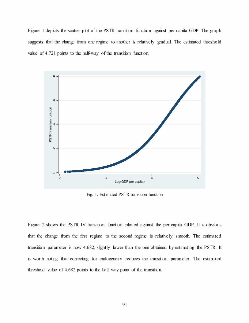
91

Figure 1 depicts the scatter plot of the PSTR transition function against per capita GDP. The graph

suggests that the change from one regime to another is relatively gradual. The estimated threshold

value of 4.721 points to the half-way of the transition function.

Fig. 1. Estimated PSTR transition function

Figure 2 shows the PSTR IV transition function plotted against the per capita GDP. It is obvious

that the change from the first regime to the second regime is relatively smooth. The estimated

transition parameter is now 4.682, slightly lower than the one obtained by estimating the PSTR. It

is worth noting that correcting for endogeneity reduces the transition parameter. The estimated

threshold value of 4.682 points to the half way point of the transition.

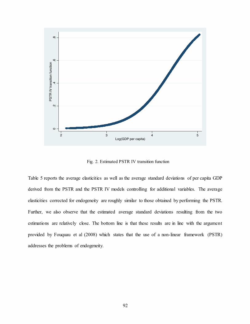
92

Fig. 2. Estimated PSTR IV transition function

Table 5 reports the average elasticities as well as the average standard deviations of per capita GDP

derived from the PSTR and the PSTR IV models controlling for additional variables. The average

elasticities corrected for endogeneity are roughly similar to those obtained by performing the PSTR.

Further, we also observe that the estimated average standard deviations resulting from the two

estimations are relatively close. The bottom line is that these results are in line with the argument

provided by Fouquau et al (2008) which states that the use of a non-linear framework (PSTR)

addresses the problems of endogeneity.

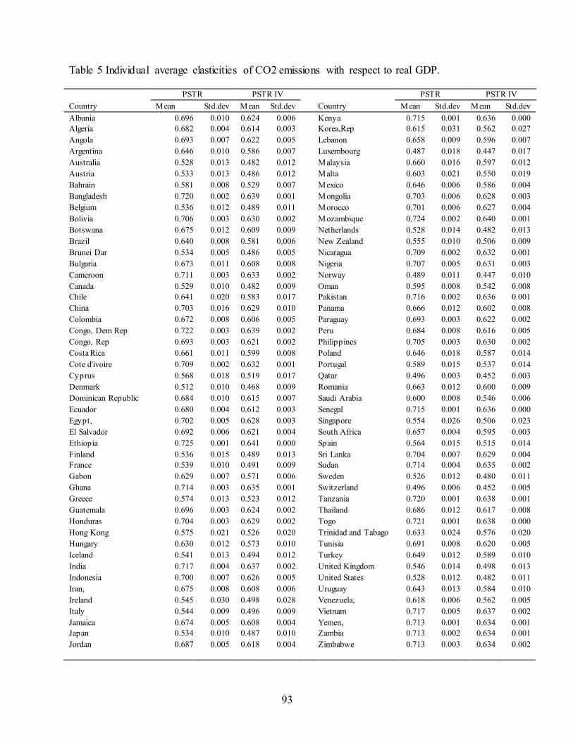
93

Table 5 Individual average elasticities of CO2 emissions with respect to real GDP. PSTR PSTR IV PSTR PSTR IV Country Mean Std.dev Mean Std.dev Country Mean Std.dev Mean Std.dev Albania 0.696 0.010 0.624 0.006 Kenya 0.715 0.001 0.636 0.000 Algeria 0.682 0.004 0.614 0.003 Korea,Rep 0.615 0.031 0.562 0.027 Angola 0.693 0.007 0.622 0.005 Lebanon 0.658 0.009 0.596 0.007 Argentina 0.646 0.010 0.586 0.007 Luxembourg 0.487 0.018 0.447 0.017 Australia 0.528 0.013 0.482 0.012 Malaysia 0.660 0.016 0.597 0.012 Austria 0.533 0.013 0.486 0.012 Malta 0.603 0.021 0.550 0.019 Bahrain 0.581 0.008 0.529 0.007 Mexico 0.646 0.006 0.586 0.004 Bangladesh 0.720 0.002 0.639 0.001 Mongolia 0.703 0.006 0.628 0.003 Belgium 0.536 0.012 0.489 0.011 Morocco 0.701 0.006 0.627 0.004 Bolivia 0.706 0.003 0.630 0.002 Mozambique 0.724 0.002 0.640 0.001 Botswana 0.675 0.012 0.609 0.009 Netherlands 0.528 0.014 0.482 0.013 Brazil 0.640 0.008 0.581 0.006 New Zealand 0.555 0.010 0.506 0.009 Brunei Dar 0.534 0.005 0.486 0.005 Nicaragua 0.709 0.002 0.632 0.001 Bulgaria 0.673 0.011 0.608 0.008 Nigeria 0.707 0.005 0.631 0.003 Cameroon 0.711 0.003 0.633 0.002 Norway 0.489 0.011 0.447 0.010 Canada 0.529 0.010 0.482 0.009 Oman 0.595 0.008 0.542 0.008 Chile 0.641 0.020 0.583 0.017 Pakistan 0.716 0.002 0.636 0.001 China 0.703 0.016 0.629 0.010 Panama 0.666 0.012 0.602 0.008 Colombia 0.672 0.008 0.606 0.005 Paraguay 0.693 0.003 0.622 0.002 Congo, Dem Rep 0.722 0.003 0.639 0.002 Peru 0.684 0.008 0.616 0.005 Congo, Rep 0.693 0.003 0.621 0.002 Philippines 0.705 0.003 0.630 0.002 Costa Rica 0.661 0.011 0.599 0.008 Poland 0.646 0.018 0.587 0.014 Cote d'ivoire 0.709 0.002 0.632 0.001 Portugal 0.589 0.015 0.537 0.014 Cyprus 0.568 0.018 0.519 0.017 Qatar 0.496 0.003 0.452 0.003 Denmark 0.512 0.010 0.468 0.009 Romania 0.663 0.012 0.600 0.009 Dominican Republic 0.684 0.010 0.615 0.007 Saudi Arabia 0.600 0.008 0.546 0.006 Ecuador 0.680 0.004 0.612 0.003 Senegal 0.715 0.001 0.636 0.000 Egypt, 0.702 0.005 0.628 0.003 Singapore 0.554 0.026 0.506 0.023 El Salvador 0.692 0.006 0.621 0.004 South Africa 0.657 0.004 0.595 0.003 Ethiopia 0.725 0.001 0.641 0.000 Spain 0.564 0.015 0.515 0.014 Finland 0.536 0.015 0.489 0.013 Sri Lanka 0.704 0.007 0.629 0.004 France 0.539 0.010 0.491 0.009 Sudan 0.714 0.004 0.635 0.002 Gabon 0.629 0.007 0.571 0.006 Sweden 0.526 0.012 0.480 0.011 Ghana 0.714 0.003 0.635 0.001 Switzerland 0.496 0.006 0.452 0.005 Greece 0.574 0.013 0.523 0.012 Tanzania 0.720 0.001 0.638 0.001 Guatemala 0.696 0.003 0.624 0.002 Thailand 0.686 0.012 0.617 0.008 Honduras 0.704 0.003 0.629 0.002 Togo 0.721 0.001 0.638 0.000 Hong Kong 0.575 0.021 0.526 0.020 Trinidad and Tabago 0.633 0.024 0.576 0.020 Hungary 0.630 0.012 0.573 0.010 Tunisia 0.691 0.008 0.620 0.005 Iceland 0.541 0.013 0.494 0.012 Turkey 0.649 0.012 0.589 0.010 India 0.717 0.004 0.637 0.002 United Kingdom 0.546 0.014 0.498 0.013 Indonesia 0.700 0.007 0.626 0.005 United States 0.528 0.012 0.482 0.011 Iran, 0.675 0.008 0.608 0.006 Uruguay 0.643 0.013 0.584 0.010 Ireland 0.545 0.030 0.498 0.028 Venezuela, 0.618 0.006 0.562 0.005 Italy 0.544 0.009 0.496 0.009 Vietnam 0.717 0.005 0.637 0.002 Jamaica 0.674 0.005 0.608 0.004 Yemen, 0.713 0.001 0.634 0.001 Japan 0.534 0.010 0.487 0.010 Zambia 0.713 0.002 0.634 0.001 Jordan 0.687 0.005 0.618 0.004 Zimbabwe 0.713 0.003 0.634 0.002

94

2.6. Concluding remarks

The purpose of this chapter was to investigate the nature of the relationship between CO2 emissions

and economic growth and to derive policy implications from the results. To this end, the Panel

Smooth Transition Regression (PSTR) model of González et al. (2005) was applied to a sample of

96 countries over the period 1984-2013 to empirically examine the relationships among CO2

emissions, economic growth.

The main focus of this study has been to verify the validity of the so-called “Environmental Kuznets

Curve” by using a more appropriate econometric technique and by incorporating energy

consumption, industrialization, urbanization, trade openness, capital expenditures as well as quality

of institutions in the model besides CO2 emissions and economic growth. In doing so, we have

expanded upon previous critiques by applying a more appropriate method and by controlling for

most of the relevant factors identified in the literature to have influence on CO2 emissions. We

discovered that the relationship between CO2 emissions and economic growth is not a U-shaped

relation. Indeed, our data demonstrate that the link between CO2 emissions and economic growth

is a non-linear relationship. More specifically, we observe that CO2 emissions tend to rise rapidly

in the early stages of economic growth, then continue to increase but at a lower rate. This finding is

in common with Aslanidis and Iranzo (2009) who also show that emissions accelerate with

economic growth in a low-income regime and then decelerate in a high-income regime.

This finding has clear policy implications, suggesting that to curb CO2 emissions in the long-run,

countries need to adopt advance abatement technology to enhance energy efficiency. Further

observation to be drawn from this result is that quality of institutions do matter for emissions-

economic growth relation. Therefore, it may be fruitful in future empirical researches that aiming to

investigate CO2 emissions-economic growth nexus to consider the potential determinants of CO2

95

emissions such as energy consumption, industrialization, urbanization, trade openness and capital

expenditures into the relation. In addition to this, it will also be important to take into account the

quality of institutions prevailing in each country in order to shed more light on the true impact of

economic growth on CO2 emissions, and thereby to provide new insight that help policy makers to

design effective environmental policies.

96

References

Ahmed, K., & Long, W. (2012). Environmental Kuznets curve and Pakistan: an empirical

analysis. Procedia Economics and Finance, 1, 4-13.

Al-Mulali, U., Weng-Wai, C., Sheau-Ting, L., & Mohammed, A. H. (2015). Investigating the

environmental Kuznets curve (EKC) hypothesis by utilizing the ecological footprint as an

indicator of environmental degradation. Ecological Indicators, 48, 315-323.

Antweiler, W., B.R. Copeland, & M.S. Taylor, (2001). Is Free Trade Good for the Environment?

American Economic Review, 877-908.

Apergis, N., Christou, C., & Gupta, R. (2017). Are there Environmental Kuznets Curves for US

state-level CO 2 emissions?. Renewable and Sustainable Energy Reviews, 69, 551-558.

Apergis, N., & Ozturk, I. (2015). Testing environmental Kuznets curve hypothesis in Asian

countries. Ecological Indicators, 52, 16-22.

Arrow, K., Bolin, B., Costanza, R., & Dasgupta, P. (1995). Economic growth, carrying capacity,

and the environment. Science, 268(5210), 520.

Aslanidis, N., & Iranzo, S. (2009). Environment and development: is there a Kuznets curve for

CO2 emissions?. Applied Economics, 41, 803-810.

Aslanidis, N., & Xepapadeas, A. (2006). Smooth transition pollution–income paths. Ecological

Economics, 57, 182-189.

Azomahou, T., Laisney, F., & Van, P. N. (2006). Economic development and CO 2 emissions: a

nonparametric panel approach. Journal of Public Economics, 90, 1347-1363.

97

Baek, J. (2015). Environmental Kuznets curve for CO 2 emissions: The case of Arctic countries.

Energy Economics, 50, 13-17.

Balaguer, J., & Cantavella, M. (2016). Estimating the environmental Kuznets curve for Spain by

considering fuel oil prices (1874–2011). Ecological Indicators, 60, 853-859.

Béreau, S., Villavicencio, A. L., & Mignon, V. (2010). Nonlinear adjustment of the real exchange

rate towards its equilibrium value: A panel smooth transition error correction modelling.

Economic Modelling, 27, 404-416.

Bessec, M., & Fouquau, J. (2008). The non-linear link between electricity consumption and

temperature in Europe: a threshold panel approach. Energy Economics, 30, 2705-2721.

Bhattarai, M., & Hammig, M. (2001). Institutions and the environmental Kuznets curve for

deforestation: a crosscountry analysis for Latin America, Africa and Asia. World

development, 29, 995-1010.

Brock, W. A., & Taylor, M. S. (2005). Economic growth and the environment: a review of theory

and empirics. Handbook of economic growth, 1, 1749-1821.

Brock, W. A., & Taylor, M. S. (2010). The green Solow model. Journal of Economic Growth, 15,

127-153.

Burton, E. (2000). The compact city: just or just compact? A preliminary analysis. Urban Studies.

37, 1969–2001.

Capello, R., Camagni, R. (2000). Beyond optimal city size: an evaluation of alternative urban

growth patterns. Urban Studies. 37, 1479–1496.

98

Chiu, Y. B. (2012). Deforestation and the environmental Kuznets curve in developing countries: A

panel smooth transition regression approach. Canadian Journal of Agricultural

Economics/Revue canadienne d'agroeconomie, 60, 177-194.

Chiu, Y. B. (2017). Carbon dioxide, income and energy: Evidence from a non-linear model.

Energy Economics, 61, 279-288.

Colletaz, G., & Hurlin, C. (2006). Threshold effects of the public capital productivity: an

international panel smooth transition approach. Document de recherche du Laboratoire

d’Economie d’Orléans.

Dijk, D. V., Teräsvirta, T., & Franses, P. H. (2002). Smooth transition autoregressive models -

a survey of recent developments. Econometric Reviews, 21, 1-47.

Dinda, S. (2004). Environmental Kuznets curve hypothesis: a survey. Ecological Economics 49,

431-455.

Du, L., Wei, C., & Cai, S. (2012). Economic development and carbon dioxide emissions in China:

Provincial panel data analysis. China Economic Review, 23, 371-384.

Duarte, R., Pinilla, V., & Serrano, A. (2013). Is there an environmental Kuznets curve for water

use? A panel smooth transition regression approach. Economic Modelling, 31, 518-527.

Ekins, P. (1997). The Kuznets curve for the environment and economic growth: examining the

evidence. Environment and planning a, 29, 805-830.

Fouquau, J., et al., 2008. The Feldstein Horioka puzzle: a panel smooth transition regression

approach. Economic Modelling 25, 284–299.

99

Fujii, H., & Managi, S. (2016). Economic development and multiple air pollutant emissions from

the industrial sector. Environmental Science and Pollution Research, 23, 2802-2812.

Galeotti, M., Lanza, A., & Pauli, F. (2006). Reassessing the environmental Kuznets curve for CO2

emissions: a robustness exercise. Ecological economics, 57(1), 152-163.

Georgiev, E., & Mihaylov, E. (2015). Economic growth and the environment: reassessing the

environmental Kuznets Curve for air pollution emissions in OECD countries. Letters in

Spatial and Resource Sciences, 8, 29-47.

González, A., Teräsvirta, T., & Dijk, D. V. (2005). Panel smooth transition regression models (No.

604). SSE/EFI Working Paper Series in Economics and Finance.

Granger, C. W., & Terasvirta, T. (1993). Modelling non-linear economic relationships. OUP

Catalogue.

Grossman, G. M., & Krueger, A. B. (1991). Environmental impacts of a North American free

trade agreement (No. w3914). National Bureau of Economic Research.

Grossman, G., & Krueger, A. (1995). Economic environment and the economic growth. Quarterly

Journal of Economics, 110, 353-377.

Hansen, B. E. (1999). Threshold effects in non-dynamic panels: Estimation, testing, and inference.

Journal of econometrics, 93, 345-368.

Harbaugh, W. T., Levinson, A., & Wilson, D. M. (2002). Re-examining the empirical evidence for

an environmental Kuznets curve. Review of Economics and Statistics, 84, 541-551.

100

Jansen, E. S., & Teräsvirta, T. (1996). Testing parameter constancy and super exogeneity in

econometric equations. Oxford Bulletin of Economics and Statistics, 58, 735-763.

Kaika, D., & Zervas, E. (2013). The Environmental Kuznets Curve (EKC) theory—Part A:

Concept, causes and the CO 2 emissions case. Energy Policy, 62, 1392-1402.

Kijima, M., Nishide, K., & Ohyama, A. (2010). Economic models for the environmental Kuznets

curve: A survey. Journal of Economic Dynamics and Control, 34, 1187-1201.

Kuznets, S. (1955). Economic growth and income inequality. The American economic review, 45,

1-28.

Liddle, B., & Messinis, G. (2015). Revisiting sulfur Kuznets curves with endogenous breaks

modeling: Substantial evidence of inverted-Us/Vs for individual OECD countries.

Economic Modelling, 49, 278-285.

Lopez-Villavicencio, A. & Mignon, V. (2011). On the impact of inflation on output growth: Does

the level of inflation matter?', Economic Modelling 33, 455-464.

Luo, G., Weng, J. H., Zhang, Q., & Hao, Y. (2017). A reexamination of the existence of

environmental Kuznets curve for CO2 emissions: evidence from G20 countries. Natural

Hazards, 85, 1023-1042.

Martino, R., & Van, P. N. (2016). Environmental Kuznets curve and environmental convergence:

A unified empirical framework for CO2 emissions. Bureau d'Economie Théorique et

Appliquée, UDS, Strasbourg.

101

Miah, M. D., Masum, M. F. H., & Koike, M. (2010). Global observation of EKC hypothesis for

CO 2, SO x and NO x emission: A policy understanding for climate change mitigation in

Bangladesh. Energy Policy, 38(8), 4643-4651.

Narayan, P. K., & Narayan, S. (2010). Carbon dioxide emissions and economic growth: panel data

evidence from developing countries. Energy Policy, 38, 661-666.

Omay, T. & Kan, E. (2010). Re-examining the threshold effects in the inflation-growth nexus with

cross-sectionally dependent non-linear panel: Evidence from six industrialized economies',

Economic Modelling 27, 996{1005.

Pesaran, M. H. (2004). General diagnostic tests for cross section dependence in panels.

Pesaran, M. H. (2006). Estimation and inference in large heterogeneous panels with a multifactor

error structure. Econometrica, 74, 967-1012.

Pesaran, M. H. (2007). A simple panel unit root test in the presence of cross‐section dependence.

Journal of Applied Econometrics, 22, 265-312.

Schmalensee, R., Stoker, T. M., & Judson, R. A. (1998). World carbon dioxide emissions: 1950–

2050. Review of Economics and Statistics, 80, 15-27.

Selden, T. M., & Song, D. (1994). Environmental quality and development: is there a Kuznets

curve for air pollution emissions?. Journal of Environmental Economics and management,

27, 147-162.

Seleteng, M., Bittencourt, M., & Van Eyden, R. (2013). Non-linearities in inflation–growth nexus

in the SADC region: A panel smooth transition regression approach. Economic Modelling,

30, 149-156.

102

Shahbaz, M., Uddin, G.S., Rehman, I.U., Imran, K., 2014. Industrialization, electricity

consumption and CO2 emissions in Bangladesh. Renew. Sustain. Energy Rev. 31, 575–

586.

Shahbaza, M., Lean, H.H., 2012. Does financial development increase energy consumption? The

role of industrialization and urbanization in Tunisia. Energy Policy 40, 473–479.

Stern, D. (2004).The rise and fall of the environmental Kuznets curve. World Development 32,

1419–1439.

Stern, D. (2015). The environmental Kuznets curve after 25 years (No. 1514). Centre for Climate

Economics & Policy, Crawford School of Public Policy, The Australian National

University.

Stern, D. I., & Common, M. S. (2001). Is there an environmental Kuznets curve for sulfur?.

Journal of Environmental Economics and Management, 41, 162-178.

Stern, D. I., Common, M. S., & Barbier, E. B. (1996). Economic growth and environmental

degradation: the environmental Kuznets curve and sustainable development. World

development, 24, 1151-1160.

Teräsvirta, T. (1994). Specification, estimation, and evaluation of smooth transition autoregressive

models. Journal of the american Statistical association, 89, 208-218.

Thanh, S. D. (2015). Threshold effects of inflation on growth in the ASEAN-5 countries: A Panel

Smooth Transition Regression approach. Journal of Economics, Finance and

Administrative Science, 20, 41-48.

103

Wang, Y., Han, R., & Kubota, J. (2016). Is there an Environmental Kuznets Curve for SO 2

emissions? A semi-parametric panel data analysis for China. Renewable and Sustainable

Energy Reviews, 54, 1182-1188.

Xu, B., & Lin, B. (2015). How industrialization and urbanization process impacts on CO 2

emissions in China: evidence from nonparametric additive regression models. Energy

Economics, 48, 188-202.

Yang, H., He, J., & Chen, S. (2015). The fragility of the Environmental Kuznets Curve: Revisiting

the hypothesis with Chinese data via an “Extreme Bound Analysis”. Ecological

Economics, 109, 41-58.

104

105

106

Chapter 3. Clean energy-growth nexus in sub-Saharan Africa: Evidence

from cross-sectionally dependent heterogeneous panel with structural

breaks23

23 A version of this chapter was published under the reference: Hamit-Haggar, M. (2016). Clean energy-growth nexus in sub-Saharan Africa: Evidence from cross-sectionally dependent heterogeneous panel with structural breaks. Renewable and Sustainable Energy Reviews, 57, 1237-1244.

107

3.1. Introduction

Determining the link between energy consumption and economic growth has become a topic studied

in depth in the field of energy economics, given the scarcity of energy resources and the fact that

energy serves as a major input in production processes. Previous studies have found a strong

correlation between energy usage and the level of economic development and growth in both

developed and developing economies (Ferguson et al. 2000). However, the presence of a strong

correlation does not necessarily imply a causal relationship. Identifying the existence and directions

of the causalities is important in the design and effectiveness of energy policies. For instance, if

there is a unidirectional causality running from energy consumption to economic growth, reducing

energy consumption could lead to a fall in economic growth. In contrast, if there is a unidirectiona l

causality running from economic growth to energy consumption, it could imply that policies

designed at reducing energy consumption may be implemented with little or no adverse impact on

economic growth.

There is a plethora of empirical work that examines the causality between energy consumption and

economic growth. Some studies are those of Narayan and Smyth (2008), Jinke et al. (2008), Bowden

and Payne (2009), Wolde-Rufael (2010a), Chandran et al. (2010), Lean and Smyth (2010), Apergis

and Payne (2010a), Payne and Taylor (2010), Wolde-Rufael (2010b), Menegaki (2011) , Dedeoglu

et al. (2014), Al-Mulali (2014), Jin and Kim (2015), Husaini and Lean (2015), Shahbaz et al. (2015)

to name only a few. Yet, there seems to be no consensus regarding the causal relationship between

energy consumption and economic growth. In general, the empirical findings have yielded rather

mixed results. The lack of consensus among the empirical works may be attributed to such factors

as differences in variable selection, model specification, sample size, the reference period and the

108

econometric approaches undertaken, among others (Zachariadis, 2007; Costantini and Martini,

2010; Apergis and Payne 2011).

For instance, Narayan and Smyth (2008) investigate the relationship between gross capital

formation, total energy consumption and real GDP in a panel of G7 countries over the period 1972–

2002. The authors find evidence of a unidirectional causality running from energy consumption to

real GDP. In a similar study, Bowden and Payne (2009) examine the causality between total energy

consumption and real GDP at the aggregate and sectoral level in the U.S. over the period 1949–

2006. They fail to reach a consensus as to the direction of causation. Dedeoglu et al. (2014) examine

the relationship between energy consumption and real gross domestic product (GDP) per capita for

the 15 former Soviet Union countries over the period 1992–2009. Their results evidence the

presence of a unidirectional causal relationship running from energy consumption to the real GDP

per capita in the long run but not in the short-run. However, they discover a bidirectional relationship

for oil importer and natural gas importer within the 15 former Soviet Union countries.

On the coal consumption-growth nexus, Jinke et al. (2008) investigate the relationship between coal

consumption and economic growth in a group of coal consuming countries (OECD and non-OECD)

over the period 1980–2005. They find a unidirectional causality running from economic growth to

coal consumption in Japan and China and no causality relationship between coal consumption and

economic growth in India, South Korea and South Africa. For the case of the United States, the

series are not even cointegrated. Similarly, Wolde-Rufael (2010a) applies a modified version of the

Granger causality test to the same sample of countries, by expanding the time span, 1965–2005. He

finds a unidirectional causality running from coal consumption to economic growth in India and

Japan while the opposite causality running from economic growth to coal consumption was found

in China and South Korea. A bi-directional causality running between economic growth and coal

109

consumption was found in the case of South Africa and the United States. In a study of this sort, Jin

and Kim (2015) examine the causal relationship between coal consumption and economic growth

for 58 countries (OECD and non-OECD countries) over the period 1971–2010. They find that coal

consumption and economic growth have a long-run equilibrium in OECD countries. In contrast, no

long-run relationship between coal consumption and economic growth is found for non-OECD

countries.

Using time series data for the period 1971–2003 and applying a bivariate and multivar ia te

framework, Chandran and colleagues (2010) study the relationship between electricity consumption

and real GDP in Malaysia. The authors discover a unidirectional causality flowing from electricity

consumption to economic growth. Lean and Smyth (2010) investigate the same issue, by examining

electricity consumption, aggregate output, exports, labor and capital in a multivariate framework.

They find a unidirectional causality running in the opposite direction, i.e., Granger causality running

from aggregate output to electricity consumption. More recently, Husaini and Lean (2015)

investigate the relationship between electricity consumption, output, and price in the manufactur ing

sector in Malaysia over the period 1978 to 2011. They find that there is a unidirectional causality

from manufacturing output to electricity consumption in the long run.

Apergis and Payne (2010a) explore the causality between renewable energy consumption and

economic growth for 13 countries within Eurasia over the period 1992–2007. They find a

bidirectional causation between renewable energy consumption and economic growth. Menegaki

(2011) investigates the causal relationship between renewable energy and economic growth for 27

European countries in a multivariate framework over the period 1997–2007. She adds variables such

as greenhouse gas emissions and employment and reports no causality between renewable energy

consumption and economic growth. Shahbaz et al. (2015) examine the relationship between

110

renewable energy consumption and economic growth by using quarterly data over the period of

1972Q1–2011Q4 and by incorporating capital and labour as potential determinants of production

function in case of Pakistan. They find evidence of a bidirectional causality between economic

growth and renewable energy consumption.

Research on the causal relationship between nuclear energy consumption and economic growth was

performed by Yoo and Jung (2005) for the case of Korea over the period 1977–2002. Their find ings

show that nuclear energy consumption causes economic growth but economic growth does not cause

nuclear energy consumption. Payne and Taylor (2010) employ the Toda and Yamamoto (1995) test

to examine the causal relationship between nuclear energy consumption and GDP growth in the

United States over the 1957–2006 period. Their results indicate that there is no causality associated

with nuclear energy consumption and economic growth. Al-Mulali (2014) investigates the causality

between nuclear energy consumption, GDP growth and CO2 emission in 30 major nuclear energy

consuming countries over the period 1990–2010. He find that nuclear energy consumption has a

positive short run causal relationship with GDP growth and a negative short run causal relationship

with CO2 emission.

While most of the existing published literature has focused on the relationship between electricity

consumption and economic growth, the relationship between coal consumption and economic

growth, the relationship between renewable energy consumption and economic growth or the

relationship between nuclear energy consumption and economic growth, virtually no published

research exists that looks into the relationship between clean energy consumption and economic

111

growth in either developed or developing economies24. In this chapter, we extend the findings of the

existing literature by applying rigorous econometric techniques to a sample of sub-Saharan African

countries to study the causality between clean energy consumption and economic growth. One of

the major limitation of earlier studies is the use of the traditional panel unit root test and panel

cointegration test (first generation of panel unit root and cointegration tests). Recent developments

in panel data analysis have raised concerns about the validity of the first generation of panel unit

root and cointegration tests which may lead to biased inferences and hence misleading results due

to lower power of the unit root and cointegration test (Andrews, 2005; Pesaran, 2006; Bai and Ng,

2010). To overcome some of the shortcomings, we employ a second generation of panel unit root

and cointegration tests, namely, the Carrion-i-Silvestre et al. (2005) panel unit root test, that

accommodates structural breaks and combines with the panel cointegration test proposed by

Westerlund and Edgerton (2008) which accounts for both cross-sectional dependence and structura l

breaks to exploit the extra power25. Furthermore, the chapter contributes to the literature by applying

a bootstrap-corrected Granger causality test to assess the short-run and the long-run dynamics

between clean energy consumption and economic growth.

We find evidence of a unidirectional causal relationship running from clean energy consumption to

economic growth. This implies that economic growth derives in part from greater clean energy

consumption, and that a decrease in clean energy consumption would be a drag on economic growth.

Therefore, the use of clean energy technologies in sub-Saharan Africa can be an economically

24 Clean energy is noncarbohydrate energy that does not produce carbon dioxide when generated. It includes hydropower and nuclear, geothermal, and solar power, among others (http://data.worldbank.org/data-catalog/world-development-indicators/wdi-2014).

25 As noted by Westerlund and Edgerton (2008), when studying macroeconomic data, cross -sectional dependencies are likely to be the rule rather than the exception, due to strong inter-economy linkages.

112

beneficial and environmentally friendly alternative to fossil energy sources26. Given this crucial

advantage accruing from the use of clean energy, and while faced with increasing demand for energy

and vulnerability to climate change, it would seem sensible for economies in sub-Saharan Africa to

set aside any pre-conceived inhibitions and to diversify their energy supply and to strengthen their

energy security by fostering the adoption of clean energy alternatives to fossil fuels27.

The roadmap for the remainder of this chapter is as follows. Section 3.2. provides the model adopted

and explains the data employed. Section 3.3. discusses and presents the results of panel unit root

and cointegration tests along with the results of a panel error correction model. Section 3.4. provides

the concluding remarks.

3.2. Model Specification and Data

Following Apergis and Payne (2009), the long-run relationship between clean energy consumption

and economic growth is given as follows:

ln 𝑌𝑖𝑡 = 𝛽0𝑖 + 𝛽1𝑖 ln 𝐶𝑖𝑡 + 𝜖𝑖𝑡 (1)

where 𝑖=1,2,...,𝑁 for each country in the panel and 𝑡=1,2,...,𝑇 refers to the time period. 𝑌𝑖𝑡 is real

GDP per capita; 𝐶𝑖𝑡 denotes clean energy consumption per capita, and 𝜖𝑖𝑡 is the error term. In order

to investigate whether there is a relationship between clean energy consumption and economic

growth, data covering the period 1971–2007 are used. The choice of the starting and ending dates

26 Africa is a stable and a safe clean energy supply, solar across all of Africa, hydro in many African countries, wind mainly in coastal areas and geothermal in the East African Rift Valley. 27 According to the International Energy Outlook 2010, in 2008, more than 70% of the sub-Saharan African populations do not have access to electricity and a large proportion of the current energy usage stems from the burning of fossil fuels (http://large.stanford.edu/courses/2010/ph240/riley2/docs/EIA-0484-2010.pdf).

113

was constrained by the availability of data. We employ annual data on clean energy consumption

per capita (aggregate consumption of hydropower and nuclear, geothermal, wind and solar

consumption, among others, in kg of oil equivalent, divided by the number of population). The real

GDP per capita series is in constant 2000 U.S. dollars and used as a proxy for economic growth.

The data on the two variables were obtained from the World Development Indicators. The countries

considered are: Cameroon, Congo (RDC), Côte d'Ivoire, Ghana, Kenya, Nigeria, South Africa,

Sudan, Togo and Zambia. Table 1 provides descriptive statistics for real GDP per capita and clean

energy consumption per capita for each country. As can be seen, the mean real GDP per capita

ranges from 3213.553 U.S. dollars in South Africa to 192.978 U.S. dollars in Congo (RDC). As for

clean energy consumption per capita, it ranges from as high as 90.207 kg of oil equivalent per capita

in Zambia to as low as 2.294 kg in Togo.

Table 1 Descriptive statistics

Real GDP (2000 US dollars per capita)

Clean energy consumption ((kg of oil

equivalent per capita)

Mean Median Std. Dev. Mean Median Std. Dev.

Cameroon 683.779 669.460 126.708

16.771 17.894 2.451

Congo Democratic

Republic. 192.978 223.623 89.165

11.998 12.523 1.712

Congo Republic. 1059.693 1092.685 170.347

8.532 9.179 4.250

Côte d'Ivoire 740.622 689.644 175.605

7.787 7.962 3.523

Ghana 244.589 239.418 32.918

28.770 30.385 7.465

Kenya 415.356 413.737 21.977

15.674 18.346 9.481

Nigeria 388.387 373.763 44.451

3.848 3.959 0.873

South Africa 3213.553 3212.637 196.584

46.811 63.719 33.896

Sudan 309.413 284.445 64.787

2.721 2.724 0.392

Togo 276.028 273.804 30.907

2.294 1.952 1.311

Zambia 412.329 396.136 89.991 90.207 78.603 32.176

114

Fig. 1 depicts the relationship between clean energy consumption and the economic growth from

1971 to 2007. There is a strong positive relationship between clean energy consumption and the

economic growth in Togo, Congo Republic, Ghana and Congo Democratic Republic, with

correlation coefficients to be (0.8480), (0.7726), (0.5949), and (0.5468) respectively. However, in

the case of Cameroon, Côte d’Ivoire and Zambia the relationship between clean energy consumption

growth and economic growth tends to decrease as income increases.

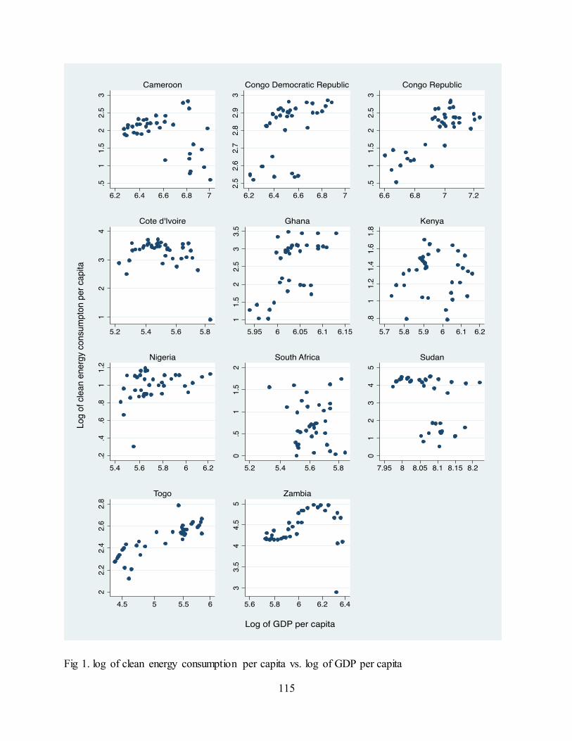
115

Fig 1. log of clean energy consumption per capita vs. log of GDP per capita

116

3.3. Econometric methodology and results

Our econometric approach to investigate the causal relationship between clean energy consumption

and economic growth consists of the following four steps. First, we investigate the stationarity

properties of the series. Second, if the series are found to be integrated of same order, we proceed

by testing for the long-run relationships among the set of integrated series. Next, we estimate the

long-run equilibrium relationship, and finally, once the long-run equilibrium relationship is

established, we employ dynamic panel causality tests to investigate the short-run and log-run

direction of causalities.

3.3.1. Cross-section dependence test

Before proceeding with investigating the order of integration of the series, a phase that is of major

concern is to test for cross-sectional dependence of the series. When cross-sectional dependence is

found, the traditional panel unit root and cointegration tests (first generation) may yield large size

distortions and thereby fail to assess clearly the integration and long-run relations among the

variables. Therefore, we start by checking for cross-sectional dependency of the data. In doing so,

we apply the cross-section dependence (CD) test developed by Pesaran (2004). Pesaran proposes a

simple diagnostic test that does not require an a priori specification of a connection or spatial matrix

and is applicable to a wide range of panel data models. The proposed test is based on a simple

average of all pair-wise correlation coefficients of the Ordinary Least Squares (OLS) residuals from

the standard panel regressions:

𝑦𝑖𝑡 = 𝛼𝑖 + 𝛽𝑖′𝑥𝑖𝑡 + 𝑢𝑖𝑡 (2)

where 𝑖=1,2,...,𝑁 indexes the cross section dimension and 𝑡=1,2,...,𝑇 the time series dimension, 𝑥𝑖𝑡

is a 𝑘𝑥1 vector of observed time-varying regressors. The individual intercepts, 𝛼𝑖 and the slope

117

coefficients, 𝛽𝑖 are defined on a compact set and are allowed to vary across 𝑖. For

each 𝑖, 𝑢𝑖𝑡~𝑖𝑖𝑑(0, 𝜎𝑖𝑢2 ) and for all 𝑡, although they could be cross-sectionally correlated. The

dependence of 𝑢𝑖𝑡 across 𝑖 could arise in a number of different ways. It could be due to spatial

dependence, omitted unobserved common components, or idiosyncratic pair-wise dependence of

𝑢𝑖𝑡 and 𝑢𝑗𝑡 for 𝑖 ≠ 𝑗. The regressors could contain lagged values of 𝑦𝑖𝑡 , be either stationary or have

unit roots. The CD test is

𝐶𝐷 = √2𝑇

𝑁(𝑁−1)∑ ∑ 𝜌𝑖𝑗

𝑁𝑗=𝑖+1

𝑁 −1𝑖=1 (3)

where 𝜌𝑖𝑗 is the sample estimate of the pair-wise correlation of the residuals

𝜌𝑖𝑗 = 𝜌𝑗𝑖 =∑ 𝑒𝑖𝑡 𝑒𝑗𝑡

𝑇𝑡=1

(∑ 𝑒𝑖𝑡2𝑇

𝑡=1 )12(∑ 𝑒𝑗𝑡

2𝑇𝑡=1 )

12

(4)

and 𝑒𝑖𝑡 is the OLS estimate of 𝑢𝑖𝑡 in Eq. (1), defined by

𝑒𝑖𝑡 = 𝑦𝑖𝑡 − �̂�𝑖 − 𝛽𝑖𝑡′ 𝑥𝑖𝑡 (5)

Pesaran shows that the CD statistic has a mean of zero for fixed values of 𝑇 and 𝑁; under a variety

of panel data models, including heterogeneous dynamic models subject to single or multip le

structural breaks in the slope coefficients and/or error variances. Table 2 displays the CD test results.

As shown in Table 2, the null hypothesis of cross-sectional independence is rejected at a 1%

significance level for the GDP, which indicates that the GDP series are cross-sectionally correlated.

For the clean energy consumption variable, the test rejects the null hypothesis of cross-sectional c

independence at a 10% significance level. The overall result favors the presence of cross sectional

118

dependence in panels28. Given the presence of cross-sectional dependence, we apply panel unit root

and panel cointegration tests which provide more powerful tests and estimates, and which have

many advantages in the presence of cross section dependence over the traditional panel unit root

and cointegration tests. This is done in the next sections.

Table 2 CD test results, cross-section correlations of the residuals in AR(p) Specification 𝑙𝑛(𝑌) 𝑙𝑛(𝐶)

Statistics Prob Statistics Prob

AR(1) 4.501*** 0.000 1.727* 0.084 AR(2) 2.929*** 0.003 1.627 0.104 AR(3) 2.897*** 0.004 1.652* 0.098

(*) and (***) denote statistical significance at the 10% and 1% levels.

3.3.2. Second generation panel unit root test

In light of the cross-sectional dependence test results, the panel unit root is checked using a second

generation of panel unit root test. We employ the Carrion-i-Silvestre et al. (2005) test to assess the

stationarity properties of the series. The benefit derived from this test is that it is general enough to

allow for heterogeneity and the possibility of multiple endogenous structural breaks and can be

adapted to accommodate cross-sectional dependence in the panel data. The model under

consideration is:

𝑦𝑖𝑡 = 𝛼𝑖 + ∑ 휃𝑖𝑘𝐷𝑈𝑖𝑘𝑡 + 𝛽𝑖𝑡 + ∑ 𝛾𝑖𝑘𝑚𝑖

𝑘 =1

𝑚𝑖

𝑘=1𝐷𝑇𝑖𝑘𝑡

∗ + 휀𝑖𝑡 (6)

28 To corroborate our findings, we apply the modified Wald statistic for groupwise heteroskedasticity in the residuals and the Lagrange multiplier (LM) tests, both tests confirm the presence of groupwise heteroskedasticity and correlation of errors across cross-sectional units. Results are not presented in the paper but can be made available upon request.

119

where 𝑖=1,2,...,𝑁 indexes the cross section dimension and 𝑡=1,2,...,𝑇 the time series dimension. The

dummy variables 𝐷𝑈𝑖𝑘𝑡 and 𝐷𝑇𝑖𝑘𝑡∗ are defined as

𝐷𝑈𝑖𝑘𝑡 = {1 𝑖𝑓 𝑡 > 𝑇𝑏𝑘𝑖

0 𝑜𝑡ℎ𝑒𝑟𝑤𝑖𝑠𝑒; 𝐷𝑇𝑖𝑘𝑡

∗ = {𝑡 − 𝑇𝑏𝑘𝑖 𝑖𝑓 𝑡 > 𝑇𝑏𝑘

𝑖

0 𝑜𝑡ℎ𝑒𝑟𝑤𝑖𝑠𝑒

with 𝑇𝑏𝑘𝑖 denoting the 𝑘 − 𝑡ℎ date of the break for the 𝑖 − 𝑡ℎ individual, 𝑘=1,2,...,𝑚𝑖 ;𝑚𝑖 ≥ 1 , and

𝛼𝑖 and 𝛽𝑖 are the parameters of the constant and time trend, respectively. And 휀𝑖𝑡 denotes the

disturbance term. The model includes individual effects, individual structural break effects and

temporal structural break effects. The test statistic is constructed by averaging the univar ia te

stationarity test in Kwiatkowski et al. (1992). The general form of the test is defined as:

𝐿𝑀(𝜆) = 𝑁−1 ∑ 𝜔𝑖−2 𝑇−2𝑁

𝑖=1 ∑ 𝑆𝑖𝑡2𝑁

𝑖=1 (7)

where 𝑆𝑖𝑡 = ∑ 휀̂𝑖𝑗 𝑡𝑗=1 denotes the partial sum process that is obtained from the estimated OLS

residuals of Eq. (6), and 𝜔𝑖2 being a consistent estimate of the long-run variance of 휀𝑖𝑡

29. By

construction, Carrion-i-Silvestre et al. (2005) test does not account for the presence of cross-section

dependence. To overcome the bias in the panel unit root testing due to cross-section dependence,

we follow the approach suggested by Maddala and Wu (1999) which recommend applying a

bootstrapped method. The application of bootstrap methods to handle cross-section dependence has

been applied in a number of studies (Narayan and Smyth, 2008; Basher and Westerlund, 2009;

Apergis and Payne, 2010b). Table 3 displays the panel stationarity test results, where breaks are

allowed in the level and the first difference of the series. The results show that the series are non-

stationary in their levels—both the asymptotic and the bootstrapped p-values reject the null

29 𝜔𝑖

2 = lim𝑇→∞

𝑇−1 𝐸(𝑆𝑖𝑡2 )

120

hypothesis of stationarity at the conventional significance level. In contrast, the stationarity test

applied to the differenced variables suggests that the null hypothesis of stationarity cannot be

rejected. Since the series are found to be integrated of the same order, the next step is to test for

cointegration in order to establish the long-run equilibrium relationship among the variables.

Table 3 Panel unit root

tests

𝑙𝑛(𝑌) 𝑙𝑛(𝐶)

Specification Statistics Proba Probb Statistics Proba Probb

Levels

Constant

8.343*** 0.000 0.000 9.231*** 0.000 0.000

Constant and trend 7.868*** 0.000 0.001 6.387*** 0.000 0.001

Break in constant 8.244*** 0.000 0.006 1.792* 0.037 0.094

First differences

Constant

1.825 0.034 0.181 0.362 0.359 0.208

Constant and trend 3.436* 0.000 0.012 1.106 0.134 0.346

Break in constant 0.528 0.299 0.336 -0.653 0.743 0.601

Notes: (a) and (b) denote probability values for a one-sided test based on the normal distribution and bootstrapped distribution,

respectively.

We use 5000 replications in the bootstrapping procedure.

We use a maximum of three breaks and the Bartlett kernel with the bandwidth of 4(T/100)2/9.

(***), (**) and (*) denote statistical significance at the 1%, 5% and 10% levels, respectively.

3.3.3. Second generation panel cointegration test

To examine whether the variables are cointegrated, we use the panel cointegration test newly-

developed by Westerlund and Edgerton (2008). The novelty of Westerlund and Edgerton (2008) test

is that it is flexible enough to allow for heteroskedastic and serially correlated errors, unit-specific

time trends, cross-sectional dependence and unknown structural breaks in both the intercept and

121

slope of the cointegrated series. It allows the structural breaks to be located at different dates for

different units. Furthermore, the distribution of the test is found to be normal and free of nuisance

parameters under the null hypothesis. As such, the Westerlund and Edgerton (2008) test has several

advantages over the first generation of panel cointegration tests. The cornerstone of Westerlund and

Edgerton (2008) test is based on the Lagrange multiplier (LM) unit root tests approach (Schmidt

and Phillips, 1992; Ahn, 1993; Amsler and Lee, 1995). The model can be set up as follows:

𝑦𝑖𝑡 = 𝛼𝑖 + 휂𝑖𝑡 + 𝛿𝑖𝐷𝑖𝑡 + 𝑥𝑖𝑡′ 𝛽𝑖 + (𝐷𝑖𝑡𝑥𝑖𝑡)′𝛾𝑖 + 𝑧𝑖𝑡 (8)

𝑥𝑖𝑡 = 𝑥𝑖𝑡−1 + 𝑤𝑖𝑡 (9)

𝑧𝑖𝑡 = 𝜆𝑖′ 𝐹𝑡 + 𝑣𝑖𝑡 (10)

𝐹𝑗𝑡 = 𝜌𝑗 𝐹𝑗𝑡−1 + 𝑢𝑗𝑡 (11)

∆𝑣𝑖𝑡 = 𝜙𝑖𝑣𝑖𝑡−1 + ∑ 𝜙𝑗𝑖𝑝𝑗=1 ∆𝑣𝑖𝑡−𝑗 + 𝑒𝑖𝑡 (12)

where 𝑖=1,2,...,𝑁 indexes the cross section dimension, 𝑡=1,2,...,𝑇 the time series dimension,

𝑗=1,2,...,𝐾 the common factors dimension, 𝑥 𝑖𝑡 is a 𝑘-dimensional vector containing the regressors

and 𝐷𝑖𝑡 is a scalar break dummy such that 𝐷𝑖𝑡 = 1 if 𝑡 > 𝑇𝑖 and zero otherwise. The parameters

𝛼𝑖 and 𝛽𝑖 represent the intercept and slope, respectively, before the break, while 𝛿𝑖 and 𝛾𝑖 represent,

respectively, the change at the time of the shift. The errors 𝑒𝑖 , 𝑣𝑖𝑡 and 𝑢𝑖𝑡 are mean zero stationary

processes which are identically and independently distributed cross-sectionally. The 𝑒𝑖𝑡 and 𝑤𝑖𝑡 are

mutually independent for all 𝑖 and 𝑡. Moreover, it is assumed that 𝜌𝑗 < 1 for all 𝑗 and 𝑇𝑖𝑏 =

𝜆𝑖𝑏𝑇 where 𝜆𝑖

𝑏 ∈ [𝑛, 𝑛 − 1] and 𝑛 ∈ (0,1).

122

The hypothesis to be tested is 𝐻0: 𝜙𝑖 = 0 for all vs. 𝐻1: 𝜙𝑖 < 0 for at least some 𝑖. To derive the

test, Westerlund and Edgerton (2008) use the Schmidt and Phillips (1992) score principle30. They

show that the score vector evaluated at the restricted maximum likelihood estimates is proportional

to the numerator of the least squares estimate of 𝜙𝑖 in the regression

∆𝑆𝑖𝑡 = 𝑎𝑖𝑡 + 𝜙𝑖𝑆𝑖𝑡−1 + ∑ 𝜙𝑗𝑖𝑝𝑗=1 ∆𝑆𝑖𝑡−𝑗 + 𝜉𝑖𝑡 (13)

where the residuals 𝑆𝑖𝑡 = 𝑦𝑖𝑡 − �̂�𝑖 − 𝛿𝑖𝐷𝑖𝑡 − 휂̂𝑖𝑡 − 𝑥𝑖𝑡′ �̂�𝑖 − (𝐷𝑖𝑡𝑥𝑖𝑡)𝛾𝑖 − �̂� 𝑖�̂�𝑡 for 𝑡=2,3,...,𝑇 with

𝑆𝑖1 = 0 . This implies that the restricted maximum likelihood estimate of 𝛼𝑖 is: �̂�𝑖 = 𝑦𝑖1 − 휂̂𝑖 −

𝛿𝑖𝐷𝑖1 − 𝑥𝑖1′ �̂�𝑖 − (𝐷𝑖1𝑥𝑖1)𝛾𝑖 and the remaining parameter estimates can be obtained by an OLS

regression of the equation

∆𝑦𝑖𝑡 = 휂̂𝑖 + 𝛿𝑖Δ𝐷𝑖𝑡 + Δ𝑥𝑖𝑡�̂�𝑖 + Δ(𝐷𝑖𝑡𝑥𝑖𝑡)′�̂�𝑖 + Δ𝑧𝑖𝑡 (14)

and �̂�𝑖, �̂�𝑖 are principal components estimates of 𝜆𝑖 and 𝐹𝑡 . Westerlund and Edgerton (2008) propose

the following LM-based statistics to test the null hypothesis

𝐿𝑀𝜙 =1

𝑁∑ 𝑇�̂�𝑖

𝑁𝑖=1

�̂�𝑖

�̂�𝑖,

𝐿𝑀𝜏 =1

𝑁∑

�̂�𝑖

𝑠.𝑒(�̂�𝑖)

𝑁𝑖=1

where �̂�𝑖 is the least squares estimate of 𝜙𝑖 in Eq. (12), 𝜎 2𝑖 =

1

𝑇∑ (Δ𝑆𝑖𝑡)2𝑇

𝑖=1 and 𝜔𝑖2 =

1

𝑇−1∑ (1 −

𝑗

𝑀+1)𝑀

𝑗=−𝑀 ∑ Δ�̂�𝑖𝑡𝑇𝑡=𝑗+1 Δ𝑆𝑖𝑡−𝑗 where 𝑀 is a kernel bandwidth parameter that determines

30 The derivation of the LM test is provided in Appendix of Westerlund and Edgerton (2007).

123

how many lagged covariances of Δ𝑆𝑖𝑡 to be estimate in the kernel. To ensure that the results provided

in this section are robust, we first test for cointegration by employing the Westerlund and Edgerton

(2008) test without allowing for structural breaks and then, we allow for level and regime shift.

Table 4 provides the results. The findings do not provide any evidence of cointegration if we ignore

the possibility of structural break. In contrast, if we allow for level breaks in the panel cointegrat ion

test, both statistics support the null hypothesis of cointegration at the conventional significance level.

However, if a regime shift is allowed, only one of the statistics favors the null hypothesis of

cointegration. Since both statistics reveal consistent results supporting the null hypothesis of

cointegration in the case of a level shift, we conclude that the series are cointegrated around a broken

intercept. Having found the presence of a long-run cointegrating relationship, the next step is to

estimate the long-run equilibrium relationship among the variables.

Table 4 Panel cointegration tests

LM𝜏 LM𝜙

Specification Statistics Prob Statistics Prob

No break -0.087 0.465 -1.039 0.149

Level break -1.627* 0.052 -4.376*** 0.000

Regime shift 0.187 0.574 -4.606*** 0.000

(***) and (*) denote statistical significance at the 1% and 10% levels, respectively.

3.3.4. Long-run elasticity estimate

Given the presence of of a long-run cointegrating relationship, four estimation techniques are

implemented to investigate the long-run effect of clean energy consumption per capita on real GDP

per capita. The Ordinary Least Squares (OLS), the Dynamic Ordinary Least Squares (DOLS)

estimator proposed by Mark and Sul (2003), the Fully Modified OLS (FMOLS) technique for

124

heterogeneous cointegrated (Pedroni, 2000, 2004) and the Dynamic Seemingly Unrelated

Regression (DSUR) estimator for multiple cointegrating regressions proposed by Mark et al. (2005).

In the case of balanced panels when the cross sectional dimension 𝑁 is substantially smaller than

the temporal dimension T (as is the case in this analysis), the DSUR technique produces very well

behaved estimators with all of the usual desirable properties (Mark et al., 2005). The results from

the estimation of Eq. (1) are shown in Table 5. Column 2 displays the point estimate and column 3

contains the standard error. The coefficient on clean energy consumption have the expected sign

and statistically significant at the 1% significance level. Since the variables are in natural logarithms,

coefficient on clean energy consumption can be interpreted as elasticity. All four estimation

techniques, OLS, DOLS, FMOLS and DSUR produce relatively similar results in terms of sign,

magnitude and statistical significance. The DSUR result indicates that a 10% increase in clean

energy consumption per capita increases real GDP per capita by about 0.91%. With respect to DOLS

and the FMOLS, both approaches provide a point estimate for clean energy consumption elasticity

of 0.093. This result is in line with Banerjee (1999) who showed that the DOLS and the FMOLS are

asymptotically equivalent for more than 60 observations. The estimate produce by OLS technique

show that the elasticity is 0.119 which is slightly greater than the value obtained by applying the

other econometrics techniques. Thus, it appears legitimate to apply the panel-based vector error

correction model to investigate the existence and directions of causalities among the variables.

Table 5 Panel long-run estimates Methods 𝛽 Standard Error

OLS 0.119*** 0.032

DOLS 0.093** 0.046

FMOLS 0.093*** 0.013

DSUR 0.091*** 0.020

(***) and (**) denote statistical significance at the 1% and 5% levels, respectively.

125

3.3.5. Panel causality test

To identify the existence and directions of causalities among the variables, we adopt the two-step

procedure of Engle and Granger (1987). In the first step, we estimate the long-run model specified

in Eq. (1) to obtain the estimated residuals and then use these residuals lagged one period as the

error correction term. A dynamic error correction is estimated

Δ ln 𝑌𝑖𝑡 = 𝜋1𝑗 + ∑ 𝜇11𝑖𝑘𝑞𝑘 =1 Δ ln 𝑌𝑖𝑡−𝑘 + ∑ 𝜇12𝑖𝑘

𝑞𝑘=1 Δ ln 𝐶𝑖𝑡−𝑘 + 𝜓1𝑖𝑒𝑐𝑡𝑖𝑡−1 + 𝜐1𝑖𝑡 (14.a)

Δ ln 𝐶𝑖𝑡 = 𝜋2𝑗 + ∑ 𝜇21𝑖𝑘𝑞𝑘 =1 Δ ln 𝐶𝑖𝑡−𝑘 + ∑ 𝜇22𝑖𝑘

𝑞𝑘=1 Δ ln 𝑌𝑖𝑡−𝑘 + 𝜓2𝑖𝑒𝑐𝑡𝑖𝑡−1 + 𝜐2𝑖𝑡 (14.b)

where ECT is the fitted value from Eq. (1) denoted by

𝑒𝑐𝑡𝑖𝑡 = ln 𝑌𝑖𝑡 − 𝛽0𝑖 − 𝛽1𝑖 ln 𝐶𝑖𝑡 (15)

Δ is the first difference operator, 𝑘 is the number of lags lengths, set at two as determined by the

Schwarz information criteria and 𝜐 is the serially uncorrelated error term. Also, to ensure that the

result is free of cross section dependence, we adopt a bootstrapped method. In terms of short- run

causality, short-run causality flows from Δ ln 𝑐 to Δ ln 𝑦 if the null hypothesis, 𝜇12𝑖𝑘 = 0∀𝑖𝑘 is

rejected. Similarly, short-run causality runs from Δ ln 𝑦 to Δ ln 𝑐 if the null hypothesis, 𝜇22𝑖𝑘 = 0∀𝑖𝑘

is rejected. With respect to the long-run causality, we tested the significance of the estimated

coefficient on the error correction term. Table 6 reports the results of the short- run and long-run

Granger-causality tests. The short-run dynamics suggests a unidirectional causality from clean

energy consumption to economic growth. With respect to the long-run dynamics, there appears to

126

be also a unidirectional causality from clean energy consumption to economic growth without any

feedback effect31.

Table 6 Panel Granger causality

Dependent variable

Independent variables

Short-run

Long-run

Δ ln(𝑌) Δ ln(𝐶)

𝐸𝐶𝑇

Δ ln(𝑌)

33.091***

(0.000)

23.690***

(0.000)

Δ ln(𝐶)

0.750

(0.686)

1.032

(0.310)

In parenthesess are the bootstrapped probability values for Wald tests with a 𝜒 2 distribution. We use 1000 replications in the bootstrapped methods. (***) denotes statistical significance at the 1%.

3.4. Concluding remarks

The study investigates the causal relationship between clean energy consumption and economic

growth using panel data for 11 sub-Saharan African countries over the period 1971-2007. We

employed the panel unit root and cointegration tests that account for the presence of cross-sectional

dependence and multiple structural breaks as well as a bootstrap-corrected Granger causality test.

The application of the panel unit root and cointegration tests reveals that there is a long-run

relationship between clean energy consumption and economic growth for a panel of sub-Saharan

Africa. The elasticity of the clean energy consumption ranges from 0.091 to 0.119, which means a

10% increase in per capita clean energy consumption increases per capita economic growth by

approximately 0.91% to 1.19%. The results from the panel error correction models indicate the

31 The estimated coefficient on the error correction term is found to be -0.349 (not reported) which suggests that when disequilibrium does occur, it will take about 2.86 years to adjust back to equilibrium.

127

presence of both short-run and long-run unidirectional causality running from clean energy

consumption to economic growth.

The existence of a unidirectional causal relationship from clean energy consumption to economic

growth has major policy implications for sub-Saharan Africa. The findings offer valuable insights

for policymakers in crafting appropriate energy policy that aims to diversify the sources of energy

and to find a stable and a safe energy supply for sub-Saharan African countries. Further, the use

clean energy use not only stimulates economic growth but also helps in addressing the internationa l

commitments to reduce CO2 emissions. As such, the use of clean energy should be taken into

consideration and promoted accordingly in the region in order to ensure sustainable economic

development.

128

References

Ahn, S. K., 1993. Some tests for unit roots in autoregressive- integrated-moving average models

with deterministic trends. Biometrica 80, 855-868.

Al-Mulali, U. (2014). Investigating the impact of nuclear energy consumption on GDP growth and

CO 2 emission: A panel data analysis. Progress in Nuclear Energy, 73, 172-178.

Amsler, C., Lee, J., 1995. An LM test for a unit root in the presence of a structural break.

Econometric Theory 11, 359-368.

Andrews, D.W. K., 2005. Cross-section Regression with Common Shocks. Econometrica 73,

1551-1585.

Apergis, N., Payne, J.E., 2009. Energy consumption and economic growth: evidence from the

Commonwealth of Independent States. Energy Economics 31, 641-647.

Apergis, N., Payne, J.E., 2010a. Renewable energy consumption and growth in Eurasia. Energy

Economics 32, 1392-1397.

Apergis, N., Payne, J.E., 2010b. Coal consumption and economic growth: Evidence from a panel

of OECD countries, Energy Policy 38, 1353-1359.

Apergis, N., Payne, J.E., 2011. A dynamic panel study of economic development and the

electricity consumption-growth nexus. Energy Economics 33, 770-781.

Bai, J., Ng, S., 2010. Panel unit root tests with cross-section dependence: A further investigation.

Econometric Theory 26, 1088-1114.

129

Banerjee, A., 1999. Panel data unit roots and cointegration: an overview. Oxford Bulletin of

economics and Statistics, 61, 607-629.

Basher, S. A., Westerlund, J., 2009. Panel cointegration and the monetary exchange rate model.

Economic Modelling 26, 506-513.

Bowden, N., Payne, J. E., 2009. The causal relationship between US energy consumption and real

output: a disaggregated analysis. Journal of Policy Modeling, 31, 180-188.

Carrion-i-Silvestre, J. L., Del Barrio-Castro, T., López-Bazo, E., 2005. Breaking the panels: an

application to the GDP per capita. Econometrics Journal 8, 159-175.

Chandran, V. G. R., Sharma, S., Madhavan, K., 2010. Electricity consumption–growth nexus: the

case of Malaysia. Energy Policy, 38, 606-612.

Costantini, V., Martini, C., 2010. The causality between energy consumption and economic

growth: A multi-sectoral analysis using non-stationary cointegrated panel data. Energy

Economics, 32, 591-603.

Dedeoglu, D., Piskin, A. (2014). A dynamic panel study of energy consumption–economic

growth nexus: evidence from the former Soviet Union countries. OPEC Energy

Review, 38, 75-106.

Engle, R.F., Granger, C.W.J., 1987. Cointegration and error correction: representation, estimation,

and testing. Econometrica 55, 251-276.

Ferguson, R., Wilkinson, W., Hill, R., 2000. Electricity use and economic development. Energy

policy, 28, 923-934.

130

Husaini, D. H., & Lean, H. H. (2015). Does Electricity Drive the Development of Manufacturing

Sector in Malaysia?. Frontiers in Energy Research, 3, 18.

Jinke, L., Hualing, S., Dianming, G., 2008. Causality relationship between coal consumption and

GDP: difference of major OECD and non-OECD countries. Applied Energy 85, 421-429.

Kwiatkowski, D., Phillips, P.C.B., Schmidt, P., Shin, Y., 1992. Testing the null hypothesis of

stationarity against the alternative of a unit root. Journal of Econometrics 54, 159-178.

Lean, H. H., Smyth, R., 2010. Multivariate Granger causality between electricity generation,

exports, prices and GDP in Malaysia. Energy, 35, 3640-3648.

Maddala, G.S., Wu, S., 1999. A comparative study of unit root tests with panel data and a new

simple test. Oxford Bulletin of Economics and Statistics 61, 631-652.

Mark, N.C., Ogaki, M., Sul, D., 2005. Dynamic Seemingly Unrelated Cointegrating Regressions.

Review of Economic Studies 72, 797-820.

Mark, N.C., Sul, D., 2003. Cointegration Vector Estimation by Panel DOLS and Long-run Money

Demand. Oxford Bulletin of Economics and Statistics 65, 655-680.

Menegaki, A., 2011. Growth and renewable energy in Europe: A random effect model with

evidence for neutrality hypothesis. Energy Economics, 33, 257-263.

Narayan, P.K., Russell, S., 2008. Energy consumption and real GDP in G7 countries: New

evidence from panel cointegration with structural breaks. Energy Economics 30, 2331-

2341.

131

Payne, J. E., Taylor, J. P., 2010. Nuclear Energy Consumption and Economic Growth in the U.S.:

An Empirical Note. Energy Sources, Part B: Economics, Planning, and Policy 5, 301-307.

Pedroni, P., 2000. Fully modified OLS for heterogeneous cointegrated panels. Advanced in

Econometrics 15, 93-130.

Pedroni, P., 2004. Panel cointegration: asymptotic and finite sample properties of pooled time

series tests with an application to the PPP hypothesis: new results. Econometric Theory 20,

597-627.

Pesaran, H.M., 2004. General diagnostic tests for cross section dependence in panels. Cambridge

Working Papers in Economics No. 435, University of Cambridge, and CESifo Working

Paper Series No. 1229.

Pesaran, H.M., 2006. Estimation and inference in large heterogeneous panels with cross section

dependence. Econometrica 74, 967-1012.

Schmidt, P., Phillips, P. C. B., 1992. LM tests for a unit root in the presence of deterministic

trends. Oxford Bulletin of Economics and Statistics 54, 257-287.

Shahbaz, M., Loganathan, N., Zeshan, M., & Zaman, K. (2015). Does renewable energy

consumption add in economic growth? An application of auto-regressive distributed lag

model in Pakistan. Renewable and Sustainable Energy Reviews, 44, 576-585.

Toda, H.Y., Yamamoto, T., 1995. Statistical inference in vector autoregressions with possibly

integrated process. Journal of Econometrics 66, 225-250.

Westerlund, J., Edgerton, D., 2007. New improved tests for cointegration with structural breaks.

Journal of Time Series Analysis 28, 188-224.

132

Westerlund, J., Edgerton, D., 2008. A simple test for cointegration in dependent panels with

structural breaks. Oxford Bulletin of Economics and Statistics 70, 665-704.

Wolde-Rufael, Y., 2010a. Bounds test approach to cointegration and causality between nuclear

energy consumption and economic growth in India. Energy Policy 38, 52-58.

Wolde-Rufael, Y., 2010b. Coal consumption and economic growth revisited. Applied Energy 87,

160-167.

Yoo, S. H., Jung, K. O., 2005. Nuclear energy consumption and economic growth in Korea.

Progress in Nuclear Energy 46, 101-109.

Zachariadis, T., 2007. Exploring the relationship between energy use and economic growth with

bivariate models: New evidence from G-7 countries. Energy Economics 29, 1233-1253.

World Bank, 2014. World Development Indicators. Accessed at:

http://www.worldbank.org/data/onlinedatabases/onlinedatabases.html.

133

134

Chapter 4: Regional and sectoral convergence of greenhouse gas

emissions in Canada32

32 Under review in Journal of Environmental Economics and Policy.

135

4.1. Introduction

There is a broader consensus in Canada and elsewhere that action is required to address mounting

challenges of climate change. According to the Fifth Assessment Report of the Intergovernmenta l

Panel on Climate Change (IPCC), global anthropogenic greenhouse gas (GHG) emissions grew on

average by 0.4 gigatonne carbon dioxide equivalent (GtCO2 eq) per year from 1970 to 2000,

whereas during the period of 2000 to 2010, emissions have risen by 1.0 GtCO2 eq on annual basis33.

The report also states that the unprecedented increase in GHG emissions observed over the last few

decades is unequivocally responsible for the discernible adverse impact on the climate and are very

likely to have contributed to the increase of global warming. A wide range of recent scientific

assessments also highlighted that most of the global warming has been caused by human activit ies,

mainly human-induced GHG emissions. GHG emissions are known to have severe adverse effects

on global average temperature, average sea level, more extreme heat waves, floods and droughts as

well as environmental refugees, among others (Lashof and Ahuja, 1990; Manne et al, 1995;

Dasgupta et al, 2007; Cayan et al, 2008).

As awareness of the stakes involved has increased, so has the will to combat, limit or prevent GHG

emissions reinforced. Admittedly, governments around the globe have made significant efforts to

effectively mitigate emissions and to address other climate change issues. International climate

negotiations among parties, such as the United Nations Framework Convention on Climate Change

(UNFCCC) was one of the most tangible proof of efforts towards this direction.

As a signatory to the UNFCCC, Canada has committed to reduce its GHG emissions to 17% below

the 2005 level by the year 2020. Although, Canada emissions represent only 1.6% of the global

33 GHG emissions are considered as the main cause of global warming and climate change.

136

GHG emissions in 2012, it is one of the highest per capita emitters. Canada’s emissions gradually

increased since 1990.34 In 2014, Canada’s total GHG emissions were estimated to be 732 of

megatonnes of carbon dioxide equivalent (Mt CO2 eq), about 20% higher of what it was in 199035.

As a result, in May 2015, the Canadian government has reiterated its intent to take ambitious action

to reduce GHG emissions by 30% below 2005 levels by 2030. However, to attain this objective, the

Canadian government understands that the need for all provinces and territories in Canada to play

their part in stabilizing atmospheric greenhouse gases is crucial in fulfilling its internationa l

emissions-reductions commitments. As such, a comprehensive plan to curb emissions across all

sectors of Canada’s economy was launched in 2016 (The Pan-Canadian Framework on Clean

Growth and Climate Change). The goal of the Pan-Canadian Framework is to build in a

collaborative approach between provincial, territorial, and federal governments in order to reduce

GHG emissions while enabling sustainable economic growth.

Mitigating GHG emissions in Canada requires a good understanding of the status of per capita GHG

emissions of each province as well as the behaviour, evolution and relative lags between sectors and

across provinces. To our knowledge, no previous empirical study has examined the distribution of

GHG emissions among Canadian provinces still less at disaggregated level. We argue that a good

understanding of the Canadian carbon footprint is important in helping implement effective

environmental policies. As it has been claimed by Apergis et al (2017), any environmental policy

design should consider regional differences in order to deliver a mitigation policy that does not

adversely affect the underlying economic structure of each region.

34 1990 is the base year required by the UNFCCC Reporting Guidelines. 35 Emissions exclude Land Use, Land Use Change and Forestry estimates.

137

Thus, the aim of this chapter is to investigate the convergence of per capita GHG emissions across

Canadian provinces for the period from 1990 to 2014. We use aggregate and sectoral (residentia l

and transportation) level data and apply the log (t) convergence test and clustering algorithm

developed by the Phillips and Sul (2007, 2009). Specifically, we would like to test whether there is

convergence, or if not, is there convergence clubs among Canadian provinces? Basically, our

question is: are Canadian provinces per capita GHG emissions converging to a unique steady state

or are they clustering around different steady states? The application of the convergence test

indicates that per capita GHG emissions do not converge to a single steady state at aggregate and at

sectoral levels. The lack of overall convergence forces us to investigate for the possibility of

convergence clubs. By controlling for the structural characteristics of provinces, we observe that

Canadian provinces’ per capita GHG emissions form distinct groups that converge to different

steady states. Moreover, the study reveals that, club members are not necessarily geographica lly

neighboring. Therefore, we do believe that the analysis presented in this chapter provide clearer

pictures of the emissions patterns either at aggregated or sectoral levels. These findings might serve

as a base for environmental policies debate and could certainly provide valuable insights for policy

makers to implement efficient local environmental policies that help achieve national emission

reduction targets.

The remainder of the chapter is organised as follows; the next section provides a brief survey of the

literature. Section 4.3. presents the methodology proposed by Phillips and Sul (2007, 2009) to test

for convergence and convergence clubs. Section 4.4. describes the data. Section 4.5. presents and

discusses the results. The last section concludes.

138

4.2. Literature review

The widening gap in per capita GHG emissions among countries has attracted a lot of attention from

both policy makers and academics in the field of environmental economics. As argued by Timils ina

(2016), the huge differences in per capita CO2 emissions between countries was one of the

contentious issues of the ongoing climate negotiations.

Over the past few decades, numerous studies have borrowed heavily from the income growth

literature to explore the convergence of emissions across countries/regions36. Common

methodological approaches, such as beta, sigma, stochastic and club convergence have been applied

in the environmental economics literature to investigate convergence of per capita emissions37.

In one of the earliest investigations in the field, List (1999) applied beta-convergence to take a closer

look at convergence of dioxide and nitrogen oxides across states in the U.S. for the period between

1929 to 1994. The finding showed that per capita emissions are converging among U.S states. In

the same vein, Romero-Ávila (2008) examined the convergence of CO2 emissions in 23 countries

of the Organisation for Economic Co-operation and Development (OECD) over the period 1960–

2002. His results supported the convergence of CO2 emissions after applying both stochastic and

deterministic convergence tests. Drawing from the economic growth literature on sigma-

36 Convergence entails that per capita emissions across countries become more equal or to some extent start narrowing over time. 37 Sigma-convergence is measured as standard deviation of the natural logarithm of per capita emissions. If this measure declines over time, then per capita emissions are converging in a sigma-sense (Barro and Sala-i-Martin, 1992). On the other hand, the stochastic-convergence tests whether time series of relative emissions per capita were characterized by a unit root. If per capita emissions are converging in a stochastic sense, then shocks to emissions are temporary and the data are stationary over time.

139

convergence, Aldy (2006) investigated whether per capita CO2 emissions have been converging

among 23 OECD countries over 1960–2000 period. The result showed that per capita emissions are

converging in a sigma sense. By considering annual data for over more than a century, spanning

from 1870–2004, Barassi et al (2011) studied the convergence of CO2 emissions within the OECD

using a stochastic convergence testing approach; they discovered that 13 out of 18 OECD countries

are indeed converging. Although most research results have provided support of convergence in per

capita emissions among industrialized countries, there is still ongoing debate when it comes to

global convergence in per capita emissions. For instance, Van (2005) applied a nonparametr ic

distribution approach to investigate the convergence in per capita emissions among 100 countries

during 1966–1996. The results offered strong evidence of convergence among industrial countries,

but no evidence of convergence was found for the entire sample. Similarly, Criado and Grether

(2011) employed a nonparametric stochastic approach to investigate the convergence of per capita

emissions among 166 countries for the period 1960–2002. They found no evidence for convergence.

On the other hand, Panopoulou and Pantelidis (2009) used a sample of 128 countries for the period

the 1960–2003 to explore convergence of per capita emissions. They employed the convergence

club test to look for evidence of convergence. Their results showed that countries tend to converge

in the early years of the sample, but two convergence clubs were formed in the later years. Many

studies thereafter have followed in the footsteps of Panopoulou and Pantelidis (2009) by applying

the Phillips and Sul (2007, 2009) methodology to detect for existence of convergence clubs among

countries and regions. For instance, Camarero et al. (2013) applied the Phillips and Sul (2007, 2009)

methodology to investigate convergence in CO2 emission intensity (emission over gross domestic

product) among OECD countries over the period 1960-2008. They identified distinctive groups of

countries that converge to different equilibria in the emission intensity for the majority of OECD

countries. Herrerias (2013) also used the convergence clubs technique to assess environmenta l

140

convergence hypothesis in carbon dioxide emissions for a large group of developed and developing

countries from 1980 to 2009. Although some countries displayed divergence, he found convergence

clubs for a large group of countries.

More recently, Apergis and Payne (2017) applied the convergence clubs approach to per capita

carbon dioxide emissions at the aggregate and sectoral level. They found evidence for presence of

multiple equilibria with respect to per capita carbon dioxide emissions at aggregate and sectoral

level. Compared with traditional convergence methodologies, the Phillips and Sul (2007, 2009)

procedure is viewed as a conditional sigma convergence that controls for the common factors.

Furthermore, the method accommodates for convergence clusters without exogenously assuming

any convergence pattern in advance; previous applied methods can only examine the panel

convergence behaviour. As such, we do believe that the Phillips and Sul (2007, 2009) convergence

test is the most appropriate approach to apply for identification of convergence clusters with respect

to per capita carbon dioxide emissions in Canada.

4.3. Methodology

4.3.1. The log (t) test

To identify convergence patterns of per capita greenhouse gas emissions across Canadian provinces

and territories at the aggregate and sectoral levels, we run the regression based technique introduced

by Phillips and Sul (2007, 2009). The novel aspect of this methodology is that, it is a nonlinear

model with a growth component and a time varying factor that allows for transitional dynamics and

capture heterogeneity across individuals and over time. Furthermore, it permits to classify

convergence clusters endogenously. Phillips and Sul’s methodology is robust to the stationarity

141

properties of the series. That is, it does not suffer from the small sample properties of traditiona l

unit root and cointegration tests. Their methodology assumes the time-varying common-fac tor

representation for the observable series 𝑋𝑖𝑡, of province 𝑖 at time 𝑡 as follows:

𝑋𝑖𝑡 = 𝜑𝑖𝜇𝑡 + 𝜖𝑖𝑡 (1)

here 𝑋𝑖𝑡 is the log value of per capita greenhouse gas emissions; 𝜑𝑖 represents the unit characterist ic

component; 𝜇𝑡 is a common component which may follow either a non-stationary stochastic trend

with drift or a trend-stationary process and 𝜖𝑖𝑡 the error term. In the specification above, the per

capita greenhouse gas emissions can be further decomposed into a common trend component 𝜇𝑡 and

an individual element 𝛿𝑖𝑡 such as:

𝑋𝑖𝑡 = (𝜑𝑖 +𝜖𝑖𝑡

𝜇𝑡) 𝜇𝑡 = 𝛿𝑖𝑡𝜇𝑡 (2)

Since it quite impossible to estimate 𝛿𝑖𝑡 from equation (2) due to over parameterization, Phillips and

Sul (2007, 2009) construct the convergence and long run equilibrium of the series based on a relative

measure of the loading coefficient as:

ℎ𝑖𝑡 =𝑋𝑖𝑡

𝑁−1 ∑ 𝑋𝑖𝑡𝑁𝑖=1

=𝛿𝑖𝑡

𝑁−1 ∑ 𝛿𝑖𝑡𝑁𝑖=1

(3)

142

note that the common component 𝜇𝑡 is removed38. Hence, ℎ𝑖𝑡 measures the transition path of

province 𝑖 to the panel average at time 𝑡. If the factor loadings 𝛿𝑖𝑡 converge to 𝛿𝑖, the relative

transition paths governed by ℎ𝑖𝑡 converges to 1 for all 𝑖 as 𝑡 → ∞. Therefore, the cross-sectional

variance of ℎ𝑖𝑡 given by 𝐻𝑡 = 𝑁−1 ∑ (ℎ𝑖𝑡 − 1)2𝑁𝑖 converges to zero as 𝑡 → ∞. To test the null

hypothesis of convergence, Phillips and Sul (2007, 2009) propose a semiparametric form for the

loading coefficient 𝛿𝑖𝑡 as follows:

𝛿𝑖𝑡 = 𝛿𝑖 + 𝜎𝑖𝜉𝑖𝑡 𝐿(𝑡)−1𝑡−𝛼 (4)

where 𝛿𝑖 is fixed, 𝜎𝑖 is an idiosyncratic scale parameter, 𝜉𝑖𝑡 ~𝑖𝑑𝑑(0,1), 𝐿(𝑡) is a slow varying

function of time and 𝛼 is a decay rate. This representation ensures that 𝛿𝑖𝑡 converges to 𝛿𝑖 for all

values of 𝛼 ≥ 0. The null hypothesis of convergence can be written as:

𝐻0: 𝛿𝑖 = 𝛿 and 𝛼 ≥ 0 vs. 𝐻𝐴: 𝛿𝑖 ≠ 𝛿 for all 𝑖 or 𝛼 < 0 (5)

To test for relative convergence, Phillips and Sul (2007, 2009) suggest estimating the following

regression by ordinary least squares.

38 Note that the common component 𝜇𝑡 is eliminated through rescaling by the panel average.

143

log (𝐻1

𝐻𝑡) − 2 log 𝐿(𝑡) = 𝑎 + �̂� log 𝑡 + 𝑢 �̂� (6)

where 𝐿(𝑡) = log(𝑡 + 1) and �̂� = 2�̂� where 𝛼 ̂is the ordinary least squares estimate of 𝛼. The null

hypothesis of convergence can be tested by applying a conventional one-sided 𝑡-test for the slope

coefficient 𝑏 ̂constructed using heteroskedasticity and autocorrelation consistent standard errors. At

the 5 % significance level, the null hypothesis of convergence is rejected if 𝑡�̂� < −1.65. Note that

the regression starts at some point 𝑡 = [𝑟𝑇], where [𝑟𝑇] is the integer part of 𝑟𝑇. Phillips and Sul

(2007, 2009) recommend 𝑟 = 1/3 as a satisfactory choice in terms of both size and power.

However, the rejection of full convergence does not imply the absence of convergence in subgroups

of the panel. Phillips and Sul (2007, 2009) propose the following algorithm for detecting

convergence clubs.

4.3.2. The clustering algorithm

Schnurbus et al. (2017) propose some minor adjustments to the original clustering algorithm of

Phillips and Sul (2007, 2009). The Schnurbus et al. (2016) adjusted algorithm is briefly outlined

below. Schnurbus et al. (2017) apply the following stepwise procedures to identify initia l

convergence clubs, to merge clubs and to establish final convergence clubs.

Step 1: Sorting

The first step consists of sorting the Hodrick and Prescott (1997)-smoothed per capita greenhouse

gas emissions series according to the last observation.

Step 2: Core group formation

144

Step 2.1: Start with the highest per capita greenhouse gas emissions, find the first two consecutive

provinces for which the log (t) regression test statistic 𝑡�̂� > −1.65. If 𝑡�̂� < −1.65 for all sequentia l

pairs of provinces, exit the algorithm and conclude that there are no convergence subgroups in the

panel39.

Step 2.2: Start with the 𝑘 = 2 provinces identified in Step 2.1, increase 𝑘 proceeding with the

subsequent province and perform the log (t) regression test. Stop increasing 𝑘 if the convergence

hypothesis fails to hold. The core group consists of the 𝑘∗ provinces that yield the highest value of

the log (t) regression test statistic.

Step 3: Extention of the initial core group

Step 3.1: Form a complementary core group of all remaining provinces not included in the core

group.

Step 3.2: Add one province at a time from the complementary to core group, (Step 3.1) to form the

core group. Run the log (t) test, if the resulting test statistic is greater than the critical value, form a

club candidate group of all provinces passing this test.

Step 3.3: An initial convergence club is obtained if the convergence hypothesis jointly holds for

both the core group and the club candidate group. Otherwise, repeat Step 3.2 until convergence

criterion is met.

Step 4: Recursion and stopping rule

39 The term log (t) stands for a parameter, which is twice the speed of convergence of this club towards the

average. The convergence test is distributed as a simple one-sided t-test with a critical value of −1.65.

145

Form a subgroup of the remaining provinces that are not sieved by Step 3. Perform the log (t) test

for this subgroup. If the test statistic is greater than −1.65, the subgroup forms the next convergence

club. Otherwise, repeat Steps 2-3 on this subgroup.

Step 5: Club merging

Perform the log (t) regression for all pairs of subsequent clubs and across formed clubs. Merge those

clubs fulfilling the convergence hypothesis jointly. Continue the procedure until no clubs can be

merged.

4.4. Data source

The data used in the study are from two sources. The first source is Environment and Climate

Change Canada (formerly known as the Environment Canada). This data set includes information

on greenhouse gas emissions, which comprise of carbon dioxide (CO2), methane (CH4), nitrous

oxide (N2O), perfluorocarbons (PFCs), hydrofluorocarbons (HFCs), sulphur hexafluoride (SF6),

and nitrogen trifluoride (NF3)). The greenhouse gas emissions are expressed as Mt CO2eq. The

second source of data is Statistics Canada from which, we collect data on population count. We

gather aggregate and sectoral levels data of all 10 Canadian provinces and territories observed

between the periods 1990-201440. The sample contains the following provinces and territories :

Newfoundland and Labrador (NL), Prince Edward Island (PE), Nova Scotia (NS), New Brunswick

(NB), Quebec (QC), Ontario (ON), Manitoba (MB), Saskatchewan (SK), Alberta (AB), British

40 Note that for the years preceding 1999, data for Nunavut and Northwest Territories are combined in a single region. After the creation of Nunavut in 1999, Nunavut data are presented separately, but we decided to combine the data for Nunavut and Northwest Territories to make a single series.

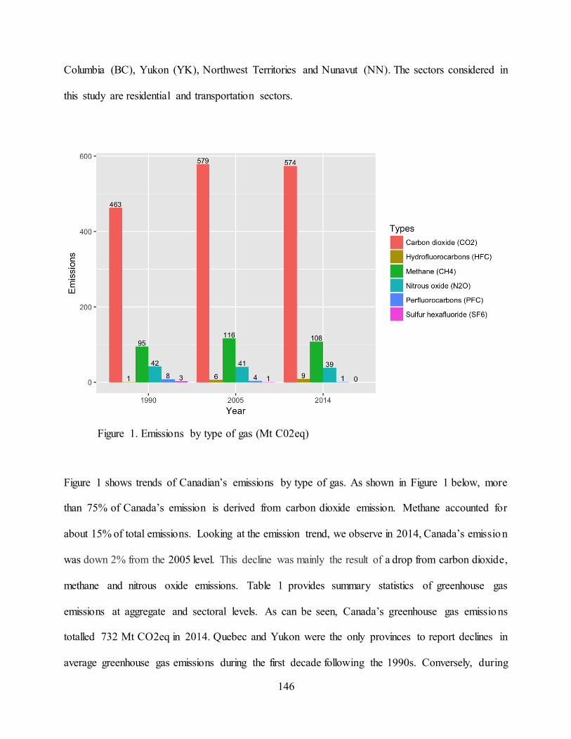
146

Columbia (BC), Yukon (YK), Northwest Territories and Nunavut (NN). The sectors considered in

this study are residential and transportation sectors.

Figure 1. Emissions by type of gas (Mt C02eq)

Figure 1 shows trends of Canadian’s emissions by type of gas. As shown in Figure 1 below, more

than 75% of Canada’s emission is derived from carbon dioxide emission. Methane accounted for

about 15% of total emissions. Looking at the emission trend, we observe in 2014, Canada’s emission

was down 2% from the 2005 level. This decline was mainly the result of a drop from carbon dioxide,

methane and nitrous oxide emissions. Table 1 provides summary statistics of greenhouse gas

emissions at aggregate and sectoral levels. As can be seen, Canada’s greenhouse gas emissions

totalled 732 Mt CO2eq in 2014. Quebec and Yukon were the only provinces to report declines in

average greenhouse gas emissions during the first decade following the 1990s. Conversely, during

147

the 2003-2014 period, all provinces and territories, except the Prairie Provinces registered decreases

in the greenhouse gas emissions. It is worth noting that greenhouse gas emissions in most provinces

were increasing during the 1990 to 2002 period, whereas, during the 2003-2014 period a large

proportion of Canadian provinces and territories are showing decline in their emissions. Is this trend

suggesting emissions are converging across Canadian provinces? The next section provides the

results of this investigation.

148

Table 1: Trends in greenhouse gas emissions in Canada

Canada Residential Transportation GHG emissions (Mt of

C02eq) Average annual

growth rate GHG emissions (Mt of

C02eq) Average annual

growth rate GHG emissions (Mt of

C02eq) Average annual

growth rate 1990 2002 2014 1990-

2002 2003-2014 1990 2002 2014 1990-

2002 2003-2014 1990 2002 2014 1990-

2002 2003-2014

Newfound and Labrador

9.58 11.79 10.56 2.27 -0.76

0.82 0.67 0.44 -1.47 -2.05

3.05 3.32 3.78 0.76 1.37

Prince Edward Island 1.96 2.05 1.80 0.42 -0.96

0.39 0.32 0.29 -1.40 -0.09

0.69 0.80 0.78 1.28 -0.13 Nova Scotia 19.97 20.72 16.58 0.36 -1.62

2.22 1.99 1.46 -0.67 -1.80

4.88 5.46 4.48 1.00 -1.40

New Brunswick 16.40 21.60 14.90 2.53 -2.93

1.15 0.77 0.59 -3.02 -1.15

4.07 5.27 3.98 2.19 -1.80 Quebec 89.14 88.59 82.68 -0.03 -0.53

8.20 6.93 4.40 -1.26 -3.50

27.96 31.78 33.74 1.11 0.53

Ontario 181.76 207.06 170.16 1.14 -1.53

18.12 19.56 21.78 0.94 1.18

48.29 60.20 60.23 1.88 0.05 Manitoba 18.68 20.38 21.48 0.77 0.49

1.68 1.32 1.25 -1.78 -0.11

7.19 7.01 8.43 -0.15 1.72

Saskatchewan 45.08 67.26 75.52 3.47 0.98

2.13 2.01 1.87 -0.27 -0.39

9.32 10.53 16.38 1.13 3.87 Alberta 175.23 229.58 273.75 2.29 1.52

6.85 8.24 9.15 1.90 1.07

22.61 31.49 45.30 2.92 3.20

British Columbia 52.88 64.59 62.94 1.73 -0.19

4.57 4.51 4.20 0.07 -0.23

18.80 23.88 24.75 2.03 0.40 Yukon 0.54 0.50 0.27 -0.07 -4.61

0.03 0.03 0.01 4.62 -2.98

0.31 0.27 0.18 -0.94 -2.69

Northwest Territories and Nunavut

1.64 2.17 1.80 3.32 -0.60

0.15 0.12 0.11 2.65 0.25

0.62 1.04 0.97 6.13 1.63

Canada 612.87 736.27 732.43 1.55 -0.02

46.31 46.47 45.56 0.20 -0.02

147.79 181.05 203.00 1.73 0.98

149

4.5. Empirical results

Table 2 reports the convergence results for aggregate per capita greenhouse gas emissions across

the Canadian provinces and territories. The top half of Table 2 displays the results for the full sample

convergence and the club clustering, while the bottom half presents the result for clubs merging. As

can be seen from the first column of Table 2, the estimated value for beta for the full convergence

is −1.114 and the corresponding t-statistic: −77.541. Based on results from the t-statistic, the null

hypothesis of full convergence can be rejected at the 5% level since the t-statistic value is below

−1.65. The absence of full convergence does not exclude the presence of convergence clubs. Thus,

we implement the club-clustering algorithm to identify provinces that satisfy the convergence clubs

criterion. The club clustering algorithm classifies four distinctive convergence clubs, with

Saskatchewan and Alberta in the first club; Newfoundland and Labrador, Nova Scotia, New

Brunswick and Northwest Territories and Nunavut in the second club; Prince Edward Island,

Ontario and British Columbia in the third club and Quebec and Yukon in the fourth. Furthermore,

we perform tests to assess whether any of formed clubs can be merged to constitute a larger

convergence club. The bottom half of Table 2 reports the testing results. The findings provide no

evidence that any subsequent clubs can be merged together to form a larger convergence club.

150

Table 2: Club convergence of per capita greenhouse gas emissions, total. Tests of club convergence

Full sample 1st Club 2nd Club 3rd Club 4th Club Newfoundland and Labrador, Prince Edward Island, Nova Scotia, New Brunswick, Quebec, Ontario, Manitoba, Saskatchewan, Alberta, British Columbia, Yukon, Northwest Territories and Nunavut (beta = −1.114, t-statistic = −77.541)

Saskatchewan, Alberta (beta = 4.445, t-statistic = 3.424)

Newfoundland and Labrador, Nova Scotia, New Brunswick, Northwest Territories and Nunavut (beta = 1.465, t-statistic = 8.157)

Prince Edward Island, Ontario, British Columbia (beta = 1.965, t-statistic = 4.750)

Quebec, Yukon (beta = 3.401, t-statistic = 3.238)

Tests of club merging 1st Club 2nd Club 3rd Club 4th Club

1st Club

−0.815 (−34.872)

−0.968 (−81.188)

−1.133 (−71.113)

2nd Club

−0.908 (−39.112)

−1.339 (−152.174)

3rd Club

−1.330 (−10.914)

4th Club

Notes: The clubs reported above have been obtained by applying the algorithm proposed by Phillips and Sul (2007, 2009). The test makes use of the critical value 𝑡0.05 ; rT−2−1=228=−1.65156 across all cases. The null hypothesis of convergence is rejected if 𝑡𝑏 < −1.65.

151

Figure 2 plots the relative transition paths of per capita greenhouse gas emissions. The relative

transition curves are meant to visually assess whether individual provinces converge relative to the

cross-sectional average over time. Full convergence occurs if the paths of all provinces

asymptotically approach one. Any point above one indicates that the province’s per capita

greenhouse gas emissions is above the cross-sectional average and vice versa.

Figure 2. Economy-wide relative transition paths of per capita greenhouse gas emissions

As shown in Figure 2, the curves eloquently capture the growth course for each province relative to

the sample average. Saskatchewan and Alberta converge to a steady state that is above the cross-

sectional average. One possible explanation that can be put forward for the high levels of per capita

152

emissions in these two provinces would be their reliance on coal-fired electricity generation as well

as oil sands and heavy oil production. Quebec and Yukon have their steady state way below the

national average. The member of the provinces in the second club reach their steady state about the

panel average. Prince Edward Island, Ontario and British Columbia, which belong to the third

convergent club, have their steady state ending to a point below the sample average.

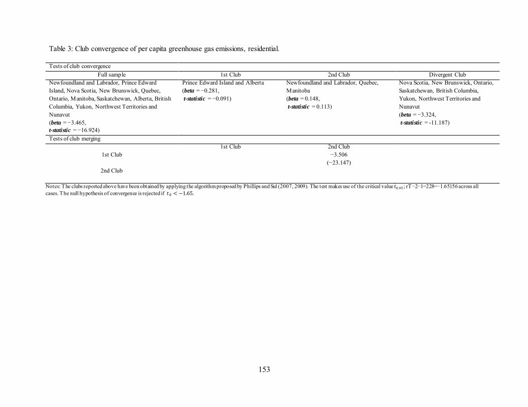
153

Table 3: Club convergence of per capita greenhouse gas emissions, residential. Tests of club convergence

Full sample 1st Club 2nd Club Divergent Club Newfoundland and Labrador, Prince Edward Island, Nova Scotia, New Brunswick, Quebec, Ontario, Manitoba, Saskatchewan, Alberta, British Columbia, Yukon, Northwest Territories and Nunavut (beta = −3.465, t-statistic = −16.924)

Prince Edward Island and Alberta (beta = −0.281, t-statistic = −0.091)

Newfoundland and Labrador, Quebec, Manitoba (beta = 0.148, t-statistic = 0.113)

Nova Scotia, New Brunswick, Ontario, Saskatchewan, British Columbia, Yukon, Northwest Territories and Nunavut (beta = −3.324, t-statistic = -11.187)

Tests of club merging 1st Club 2nd Club

1st Club

−3.506 (−23.147)

2nd Club

Notes: The clubs reported above have been obtained by applying the algorithm proposed by Phillips and Sul (2007, 2009). The test makes use of the critical value 𝑡0.05 ; rT−2−1=228=−1.65156 across all cases. The null hypothesis of convergence is rejected if 𝑡𝑏 < −1.65.

154

Table 3 reports the results for the residential sector’s per capita greenhouse gas emissions across the

Canadian provinces and territories. Clearly, the null hypothesis of full convergence is rejected at the

5% level. The divergence of per capita greenhouse gas emissions for the whole sample does not,

however, rule out the possibility of convergence clubs. The convergence clubs tests results indicate

the presence of two convergent clubs and one divergent set of provinces. The first club consists of

Prince Edward Island and Alberta. The second club includes Newfoundland and Labrador, Quebec

and Manitoba. The divergent set of province is made up of Nova Scotia, New Brunswick, Ontario,

Saskatchewan, British Columbia, Yukon, Northwest Territories and Nunavut.

When tested for clubs mergers, the t-statistic value for club merging, −23.147, is significantly

smaller than −1.65, strongly rejecting the null hypothesis of clubs merging.

Figure 3. Residential relative transition paths of per capita greenhouse gas emissions

155

Figure 3 displays the paths of the relative convergence across Canadian residential sector emissions.

The emissions trajectories for the member of first club (Prince Edward Island and Alberta) appear

to be increasing with respect to the sample average. The increasing level of greenhouse gas

emissions for residential sector in Alberta can be explained by the size of homes in Alberta. In

Alberta, homes built between 2000 and 2010 are approximately 37 per cent larger than those built

from 1960 to 1980. Larger homes require more energy for heating, thus more emissions to be

released. However, for the case of Prince Edward, Island, it can be explained by Island homes burn

fossil fuels like light fuel oil, heavy fuel oil, diesel, and propane to produce heat or electricity. These

fuels are known to generate more greenhouse gas emissions. Several additional observations are

worth mentioning. In most provinces, greenhouse gas emissions remain steadily constant up to 2004

and then start to increase or decline in certain cases.

156

Table 4: Club convergence of per capita greenhouse gas emissions, transportation.

Tests of club convergence

Full sample 1st Club 2nd Club 3rd Club 4th Club Divergent Club Newfoundland and Labrador, Prince Edward Island, Nova Scotia, New Brunswick, Quebec, Ontario, Manitoba, Saskatchewan, Alberta, British Columbia, Yukon, Northwest Territories and Nunavut (beta = −1.173, t-statistic= −101.910)

Saskatchewan, Northwest Territories and Nunavut (beta = 0.083, t-statistic = 2.869)

Newfoundland and Labrador, Alberta (beta =1.465, t-statistic = 8.157)

New Brunswick, Manitoba, Yukon (beta = 0.759, t-statistic = 1.907)

Quebec, Ontario, British Columbia (beta = 0.267, t-statistic = 4.461)

Prince Edward Island, Nova Scotia (beta = −7.662, t-statistic = −3.526)

Tests of club merging 1st Club 2nd Club 3rd Club 4th Club

1st Club

-0.302 (-5.377)

-1.358 (-133.745 )

-1.179 (-127.063)

2nd Club

-1.246 (-12.334)

-0.962 (-21.981)

3rd Club

0.147 (4.212)

4th Club

Notes: The clubs reported above have been obtained by applying the algorithm proposed by Phillips and Sul (2007, 2009). The test makes use of the critical value 𝑡0.05 ; rT−2−1=228=−1.65156 across all cases. The null hypothesis of convergence is rejected if 𝑡𝑏 < −1.65.

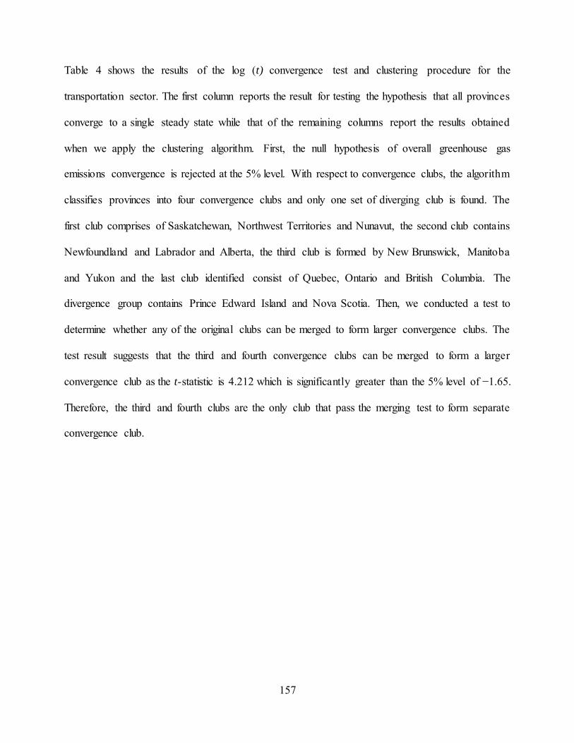
157

Table 4 shows the results of the log (t) convergence test and clustering procedure for the

transportation sector. The first column reports the result for testing the hypothesis that all provinces

converge to a single steady state while that of the remaining columns report the results obtained

when we apply the clustering algorithm. First, the null hypothesis of overall greenhouse gas

emissions convergence is rejected at the 5% level. With respect to convergence clubs, the algorithm

classifies provinces into four convergence clubs and only one set of diverging club is found. The

first club comprises of Saskatchewan, Northwest Territories and Nunavut, the second club contains

Newfoundland and Labrador and Alberta, the third club is formed by New Brunswick, Manitoba

and Yukon and the last club identified consist of Quebec, Ontario and British Columbia. The

divergence group contains Prince Edward Island and Nova Scotia. Then, we conducted a test to

determine whether any of the original clubs can be merged to form larger convergence clubs. The

test result suggests that the third and fourth convergence clubs can be merged to form a larger

convergence club as the t-statistic is 4.212 which is significantly greater than the 5% level of −1.65.

Therefore, the third and fourth clubs are the only club that pass the merging test to form separate

convergence club.

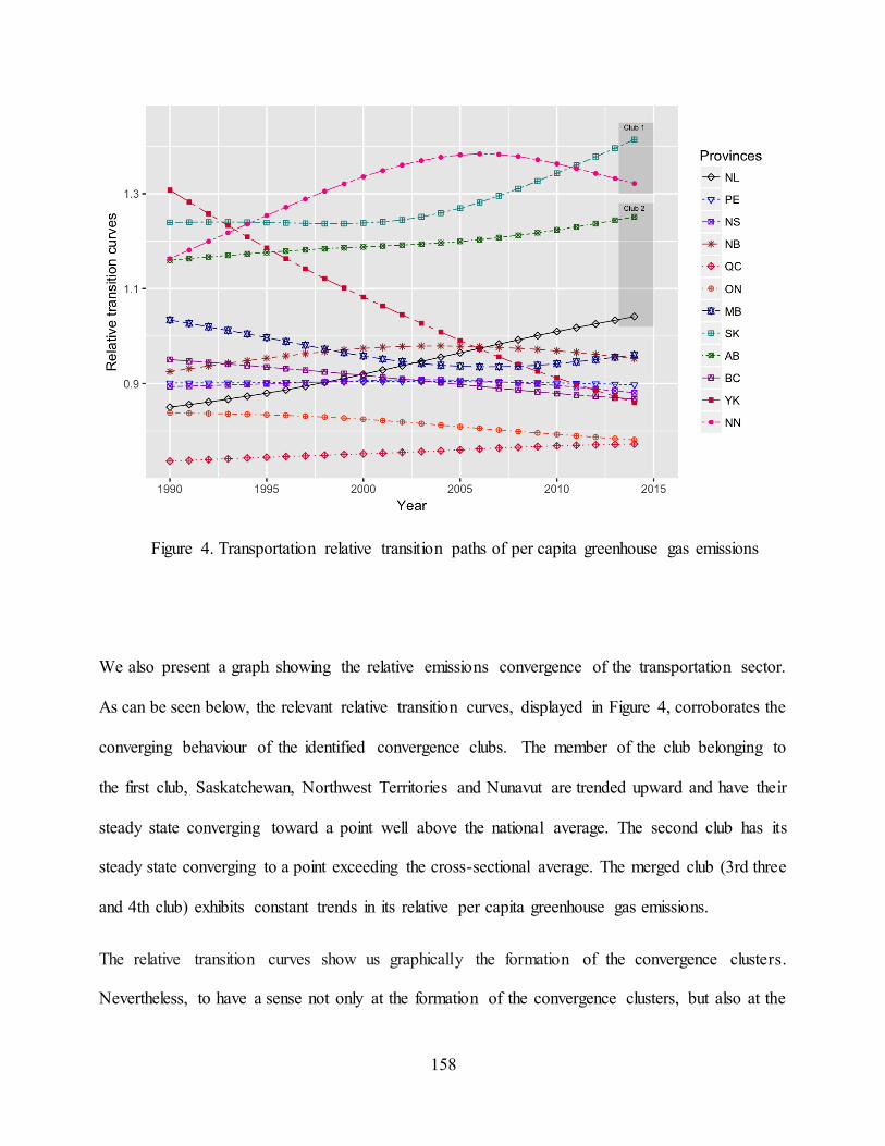
158

Figure 4. Transportation relative transition paths of per capita greenhouse gas emissions

We also present a graph showing the relative emissions convergence of the transportation sector.

As can be seen below, the relevant relative transition curves, displayed in Figure 4, corroborates the

converging behaviour of the identified convergence clubs. The member of the club belonging to

the first club, Saskatchewan, Northwest Territories and Nunavut are trended upward and have their

steady state converging toward a point well above the national average. The second club has its

steady state converging to a point exceeding the cross-sectional average. The merged club (3rd three

and 4th club) exhibits constant trends in its relative per capita greenhouse gas emissions.

The relative transition curves show us graphically the formation of the convergence clusters.

Nevertheless, to have a sense not only at the formation of the convergence clusters, but also at the

159

spatial agglomeration of each clubs, we show the geographical connection between the members of

the convergence clubs.

Aggregate (a).

160

Residential (b).

161

Transportation (c).

Map 1 displays the geographical distribution of the clubs for aggregate, residential and

transportation. It is worth to note that the figures in Map 1 are plotted based on the convergence -

clustering algorithm testing results. Firstly, convergence club for aggregate seem to be spatially

concentrated at least for the first two clubs. For instance, Alberta and Saskatchewan do not only

share oil sands and heavy oil production but also share geographical connection. The provinces in

the second club are also connected on geographic lines. A closer look over the geographica l

distribution of the clubs in the residential sector show also a geographical link for the set of divergent

162

four provinces in western regions. With respect to the spatial connection of the transportation sector,

it can be observed that the provinces in the first and the fourth clubs are also geographica lly

connected.

4.6. Conclusions

In this chapter, we examined the environmental convergence hypothesis among Canadian provinces

and territories. To serve this objective, we apply the testing approach of Phillips and Sul (2007,

2009). This methodology uses a non-linear factor model with a common and an idiosyncrat ic

component allowing for technical progress heterogeneity across provinces. More specifically, we

investigate whether per capita GHG emissions converge at aggregate and sectoral level for the

period 1990 to 2014.

First, the testing results reject the null hypothesis of full convergence at aggregate as well as sectoral

levels. To investigate the existence of segmentation in per capita GHG emissions across Canadian

provinces and territories. We apply the clustering procedure to the aggregated and sectoral level

data, the application of the convergence clubs testing identifies groups of provinces and territories

that converge to different equilibria in aggregated per capita GHG emissions. The first club

comprises of Saskatchewan and Alberta; these two provinces are the country’s largest emitters .

Indeed, in 2013, 91% of oil produced in Canada is from Alberta and Saskatchewan, which explain

in part the above national average emissions for these two provinces. The province of Newfoundland

and Labrador, Nova Scotia, New Brunswick and Northwest Territories and Nunavut form the second

group. The third group comprises of Prince Edward Island, Ontario and British Columbia and

finally, Quebec and Yukon come in the fourth club.

163

In terms of per capita GHG emissions convergence for residential sector, the club convergence

algorithm identifies the presence of two convergent clubs and one divergent set of provinces. With

respect to the convergence of per capita GHG emissions for transportation sector, the clustering

algorithm classifies provinces in four convergence clubs and one set of diverging province.

Therefore, we argue that the presence of multiple convergent clubs suggests that to achieve the

emissions reduction targets, the federal and provincial governments should design specific

environmental policy that equitably share the burden of GHG emissions among provinces that

enable sustainable development, while reaching the national emission reduction goals.

164

References

Aldy, J. E. (2006). Per capita carbon dioxide emissions: convergence or divergence?.

Environmental and Resource Economics, 33(4), 533-555.

Apergis, N., & Payne, J. E. (2017). Per capita carbon dioxide emissions across US states by sector

and fossil fuel source: Evidence from club convergence tests. Energy Economics.

Apergis, N., Payne, J. E., & Topcu, M. (2017). Some empirics on the convergence of carbon

dioxide emissions intensity across US states. Energy Sources, Part B: Economics,

Planning, and Policy, 1-7.

Barassi, M. R., Cole, M. A., & Elliott, R. J. (2011). The stochastic convergence of CO 2

emissions: a long memory approach. Environmental and Resource Economics, 49(3), 367-

385.

Barro, R. J., & Sala-i-Martin, X. (1992). Convergence. Journal of political Economy, 100(2), 223-

251.

Camarero, M., Picazo-Tadeo, A. J., & Tamarit, C. (2013). Are the determinants of CO 2 emissions

converging among OECD countries?. Economics Letters, 118(1), 159-162.

Cayan, D. R., Bromirski, P. D., Hayhoe, K., Tyree, M., Dettinger, M. D., & Flick, R. E. (2008).

Climate change projections of sea level extremes along the California coast. Climatic

Change, 87, 57-73.

Criado, C. O., & Grether, J. M. (2011). Convergence in per capita CO 2 emissions: a robust

distributional approach. Resource and energy economics, 33(3), 637-665.

165

Dasgupta, S., Laplante, B., Meisner, C., Wheeler, D., & Yan, J. (2009). The impact of sea level

rise on developing countries: a comparative analysis. Climatic change, 93(3), 379-388.

Herrerias, M. J. (2013). The environmental convergence hypothesis: Carbon dioxide emissions

according to the source of energy. Energy Policy, 61, 1140-1150.

Hodrick, R. J., & Prescott, E. C. (1997). Postwar US business cycles: an empirical investigation.

Journal of Money, credit, and Banking, 1-16.

Lashof, D. A., & Ahuja, D. R. (1990). Relative contributions of greenhouse gas emissions to

global warming. Nature, 344(6266), 529-531.

List, J. A. (1999). Have air pollutant emissions converged among US regions? Evidence from unit

root tests. Southern Economic Journal, 144-155.

Manne, A., Mendelsohn, R., & Richels, R. (1995). MERGE: A model for evaluating regional and

global effects of GHG reduction policies. Energy policy, 23(1), 17-34.

Panopoulou, E., & Pantelidis, T. (2009). Club convergence in carbon dioxide emissions.

Environmental and Resource Economics, 44(1), 47-70.

Phillips, P. C., & Sul, D. (2007). Transition modeling and econometric convergence tests.

Econometrica, 75(6), 1771-1855.

Phillips, P. C., & Sul, D. (2009). Economic transition and growth. Journal of Applied

Econometrics, 24(7), 1153-1185.

Romero-Ávila, D. (2008). Convergence in carbon dioxide emissions among industrialised

countries revisited. Energy Economics, 30(5), 2265-2282.

166

Schnurbus, J., Haupt, H., & Meier, V. (2017). Economic Transition and Growth: A Replication.

Journal of Applied Econometrics, 32(5), 1039-1042.

Timilsina, G. R. (2016). Will global convergence of per-capita emissions lead the way to meeting

the UNFCCC goal?. Carbon Management, 7(3-4), 125-136.

Van, P. N. (2005). Distribution dynamics of CO2 emissions. Environmental and Resource

Economics, 32(4), 495-508.

167

168

169

General conclusion

Main results

The rapid increase in global greenhouse emissions in recent times have ignited the debate about the

consequences of emissions on the economy and the society. Now, there is a general agreement by

scholars and policy makers that sustainable development cannot be achieved without a clear

understanding of the interaction between environment, economic, political and socio-cultura l

characteristics of countries. As such, many countries throughout the world have started to integrate

socio-economic, political and environmental considerations into their development agenda.

This thesis tries to empirically investigate the role played by socioeconomic, socio-demographic

characteristics and contextual factors on individuals’ tendency to contribute toward environmenta l

quality improvements. And then move on by exploring the link between environmental degradation

and economic growth as well as the factors that helped in reducing environmental degradation in

developed and developing countries.

The first chapter seeks to examine the societal bases of public concern related to environmenta l

quality by exploring the factors behind individuals’ engagement in environmental protection. It

applies a multilevel modeling approach on individual and contextual data. The results from this

analysis show that both individual and contextual level factors played a major role in explaining

individuals’ involvement in environment protection. More specifically, the study reveals that,

individual level covariates accounts for about 80.5% of total variability in explaining environmenta l

awareness across nations. The remaining 19.5% is attributable to country level characteristics.

At the individual level, results show that determinants, such as education, relative income, post-

materialistic values, religious beliefs and adhesion to environmental organization are associated

170

with high levels of willingness to pay to protect the environment. Country level covariates show

that population density as well as the quality of institutions contributed to individuals’ willingness

to pay for a better environmental quality. In sum, the findings from this study reveals that the

disparities observed in the willingness to pay to protect the environment between countries can arise

from both individual and contextual level factors. As it is evidenced by the impact of individua ls

and country level covariates on individuals’ willingness to pay for environmental protection. The

findings arising from this chapter may have major implications for economic and policy practice. It

can be argued that organized and educated individuals can change the way government implements

environmental policies.

The second chapter tries to contribute to the existing literature by empirically assessing the impact

of economic growth, energy consumption, trade openness, industrialization, urbanization and

quality of institutions on CO2 emissions. The overarching objectives of this chapter is to investiga te

whether or not the inverted U-shaped relationship between economic growth and environmenta l

degradation is supported by the data, and then, it attempts to assess the role played by energy

consumption, trade openness, industrialization, urbanization and quality of institutions in that

relation. To serve these objectives, we apply the panel smooth transition regression (PSTR) model

of González et al. (2005) to test the EKC hypothesis. The investigation provides no evidence of the

inverted U-shaped relationship between economic growth and environmental degradation in both

developing and developed countries. Instead, a non-linear relationship is found between CO2

emissions and economic growth. In other words, the result shows that CO2 emissions tend to rise

rapidly in the early stage of economic growth, then continue to increase but at a lower rate in the

later stage. With respect to the effects of the other covariates on CO2 emissions, we found relative ly

similar impacts than results reported by numerous previous studies. More formally, we observed

171

that energy consumption, industrialization and trade openness present statistically significantly

impact on CO2 emissions in both developing and developed countries. However, the result did not

provide any evidence with regard to the impact of urbanization on CO2 emissions. With regard to

the effect of democratic accountability of the government and government stability, it appears that

both democratic accountability and government stability lead to CO2 emissions reduction rates

mainly in developed countries.

In chapter 3, we explore whether or not clean energy technologies bolster economic growth. It is

argued that renewable energy plays an important role in energy security, in improving health and

quality of life by maintaining or enhancing the quality of the environment. But the question that

remains to be understood is whether the adoption of clean energy technologies cause growth. To

investigate this issue, we make use of data from 11 sub-Saharan African countries over the period

1971-2007 and apply a second generation of panel unit root and cointegration testing procedure that

account for the presence of cross-sectional dependence and multiple structural breaks. The empirica l

evidence shows that there is a short and long-run relationship between clean energy consumption

and economic growth. The finding indicates that a 10% increase in per capita clean energy

consumption increases per capita economic growth by approximately 0.91% to 1.19%. Furthermore,

the result of panel error correction model points towards the presence of unidirectional causality

running from clean energy consumption to economic growth in both short and long run. These

findings offer valuable insights for policymakers in crafting appropriate energy policy that aims to

diversify the sources of energy and to find a stable and a safe energy supply for sub-Saharan African

countries that will help create jobs and eradicate poverty.

Chapter 4 tests for convergence in emissions of greenhouse gases among Canadian provinces by

using aggregate and sectoral level data for the period 1990 to 2014. In so doing, we employ the

172

Phillips and Sul (2007) notion of convergence, which allows technical progress to vary across

provinces. We wonder whether Canadian’s per capita greenhouse gases emissions converge to a

single steady state or do cluster around multiple steady states. First, we test whether the per-capita

greenhouse gases emissions in Canadian provinces share a common trend, and if so, have these

provinces experienced convergence in the greenhouse gases emissions. The testing results reject the

null hypothesis of full convergence across Canadian provinces at aggregate and sectoral levels.

Then, we implemented the clustering algorithm to the aggregated and sectoral level data. The

convergence clubs testing identifies groups of provinces that converge to different equilibria in per

capita greenhouse gases emissions. We observe that per capita emissions of Canada’s largest

emitters (Saskatchewan and Alberta) form a single club. This can be explained by the fact that these

two provinces are Canada most energy intensive provinces. About, 91% of oil produced in Canada

is from these two provinces. The study also identifies the presence of multiples convergence clubs

at the sectoral level.

Policy implications and future research

As environmental quality is the responsibility of all those whose actions have affected the

environment. Public, government and non-governmental organizations are more than ever believe

that collaborative efforts are needed to mitigate the effects of human activities on global

environmental degradation. From a management perspective, the challenge is how to implement

policies that protect environmental quality without dampening the economic development. Analys is

conducted in this thesis focuses on the determinants of individuals’ attitudes towards preventing

environmental damage as well as the determinants of environmental degradation and concludes on

how a better understanding of the sources behind environmental pollution can help define economic

and environmental policies that may help achieve sustainable development.

173

Concerning the investigation of the role played by socioeconomic, socio-demographic

characteristics and contextual factors, the analysis concludes that both individuals and contextua l

level covariates are correlated with individuals’ willingness to contribute toward environmenta l

quality improvements. For instance, the study reveals that educated individuals are more concerned

about the environment than not educated ones. This finding suggests that environmental protection

agency and governments should adequately sensitize the public on the need for attitudinal change

towards environmental protection through education. Besides, the fact that richer people are more

likely to pay for the restoration of the environment recommends that if a program to collect funds

can be designed and implemented, it could help to alleviate the financial burden of the government

while addressing environmental issues. On the other hand, the result also suggests that an

improvement of the democratization process of a country shapes pro-environmental behaviour and

attitudes. Although it is argued that some contextual factors may influence environmenta l

protection, it is not yet clear how they influence individuals’ environmental awareness. More

research work is needed to determine if contextual features are more or less conducive to

individuals’ willingness to pay to protect the environment protection.

One of the observations arising out of this research is that the presumption that economic growth is

not a threat to the environment is not supported by the data. A consequential implication of this

conclusion is that efforts by governments and international bodies to improve environmental quality

should therefore be seen as a priority. They should be resolute in the implementation and

enforcement of environmental laws and regulations in a manner that guarantees sustained econo mic

growth. As economic development and environmental regulation differ among countries, one may

argue that the inverted U-shaped relation found in previous studies might be attributable to

polynomial curve fitting rather than to underlying structural relationships. It is well known that

174

countries’ environmental data collection begins early 1970’s which render cross country

examination more challenging since many developed countries had already initiated downward

trends for most pollutants. As such, in future research, it may be fruitful to focus on a country study

by employing disaggregate level data. Since it may shed additional insight on the impact of

economic growth on the environment degradation, and thereby provide new information to help

policy makers to design appropriate economic and environmental policies.

With respect to the relationship between clean energy consumption and economic growth, the

analysis demonstrates that there is a unidirectional Granger causality flowing from clean energy

consumption to economic growth. Given the causal effect that clean energy consumption exert on

economic growth, African countries should adopt clean technologies to foster economic growth.

While there is a high initial costs of adopting clean technologies, it use will significantly increase

access to electricity for a high proportion of the population, increase their productivity and

competitiveness which lead to job creation, lower poverty rates and long term food security. Even

though the study establishes empirical evidence for the effect of clean energy consumption on

economic growth, it is not without limitations. Some important variables may have been left out

from the models. Variables, such as trade openness and capital formation. Additionally, this study

was conducted with a sample of 11 sub-Saharan African countries. It is therefore suggested that

further research can be conducted with larger samples size and control for some relevant covariates,

so as to improve the generalization of the result and eliminate possible sampling bias.

The presence of multiple convergent clubs found among Canadian provinces suggests that to better

align emissions reduction across provinces, the federal and provincial governments should design

specific environmental policy that equitably share the burden of greenhouse gases emissions among

175

provinces that enable sustainable development, while reaching the national emission reduction

goals.

176

Table of Contents

General introduction.......................................................................................................................2

Chapter 1. A multilevel analysis of the determinants of willingness to pay to prevent environmental pollution across countries.........................................................................................24

1.1. Introduction ...........................................................................................................................25

1.2. Related Literature ..................................................................................................................29

1.2.1. The post-materialist values thesis ........................................................................................ 29

1.2.2. The affluence hypothesis ..................................................................................................... 30

1.2.3. The global environmentalism theory .................................................................................... 31

1.3. Econometric framework ........................................................................................................32

1.4. Data .......................................................................................................................................35

1.4.1. The World Values Survey .................................................................................................... 35

1.4.2. Individual level covariates .................................................................................................. 36

1.4.3. Country level covariates ..................................................................................................... 39

1.5. Results and discussion...........................................................................................................43

1.5.1. Full sample of countries...................................................................................................... 43

1.5.2. Developed countries ........................................................................................................... 49

1.5.3. Developing countries .......................................................................................................... 53

1.5.4. Robustness analysis of the results ........................................................................................ 57

1.6. Conclusions ...........................................................................................................................59

References ....................................................................................................................................63

Chapter 2. On the relationship between CO2 emissions and economic growth: Evidence from panel smooth transition regression ...................................................................................................72

2.1. Introduction ...........................................................................................................................73

2.2. Brief literature review ...........................................................................................................75

2.3. Econometric methodology.................................................................................................77

2.3.1. PSTR model specification.................................................................................................... 77

2.3.2. Model specification and testing procedure ........................................................................... 80

2.3.3. PSTR estimates and endogeneity ......................................................................................... 81

2.4. Data sources and variable definitions....................................................................................82

2.5. Empirical results....................................................................................................................84

2.5.1. Linearity and no remaining non-linearity test results ............................................................ 84

2.5.2. PSTR estimation results ...................................................................................................... 85

2.6. Concluding remarks ..............................................................................................................94

References ....................................................................................................................................96

177

Chapter 3. Clean energy-growth nexus in sub-Saharan Africa: Evidence from cross-sectionally dependent heterogeneous panel with structural breaks ..................................................................106

3.1. Introduction .........................................................................................................................107

3.2. Model Specification and Data .............................................................................................112

3.3. Econometric methodology and results ................................................................................116

3.3.1. Cross-section dependence test ........................................................................................... 116

3.3.2. Second generation panel unit root test ............................................................................... 118

3.3.3. Second generation panel cointegration test ........................................................................ 120

3.3.4. Long-run elasticity estimate .............................................................................................. 123

3.3.5. Panel causality test........................................................................................................... 125

3.4. Concluding remarks ............................................................................................................126

References ..................................................................................................................................128

Chapter 4: Regional and sectoral convergence of greenhouse gas emissions in Canada ..............134

4.1. Introduction .........................................................................................................................135

4.2. Literature review .................................................................................................................138

4.3. Methodology .......................................................................................................................140

4.3.1. The log (t) test .................................................................................................................. 140

4.3.2. The clustering algorithm ................................................................................................... 143

4.4. Data source ..........................................................................................................................145

4.5. Empirical results..................................................................................................................149

4.6. Conclusions .........................................................................................................................162

References ..................................................................................................................................164

General conclusion .....................................................................................................................169

178

Abstract

This thesis comprises four empirical essays on environmental and development economics. In the first chapter, we examine to what extent individual and contextual level factors influence individua ls to contribute financially to prevent environmental pollution. We find that rich people, individua ls with higher education, as well as those who possess post-materialist values are more likely to be concerned about environmental pollution. We also observe the country in which individuals live matter in their willingness to contribute. More precisely, we find democracy and government stability reduce individuals’ intention to donate to prevent environmental damage mainly in developed countries. The second chapter deals with the relation between economic growth and environmental degradation by focusing on the issue of whether the inverted U-shaped relation exist. The study discloses no evidence for the U-shaped relation. However, the empirical result points toward a non-linear relationship between environmental degradation and economic growth, that is, emissions tend to rise rapidly in the early stages with economic growth, and then emissions continue to increase but a lower rate in the later stages. The third chapter investigates the long-run as well as the causal relationship between energy consumption and economic growth in a group of Sub-Saharan Africa. The result discovers the existence of a long-run equilibrium relationship between clean energy consumption and economic growth. Furthermore, the short-run and the long-run dynamics indicate unidirectional Granger causality running from clean energy consumption to economic growth without any feedback effects. The last chapter of this thesis concerns with convergence of emissions across Canadian provinces. The study determines convergence clubs better characterizes Canadian’s emissions. In other words, we detect the existence of segmentat ion in emissions across Canadian provinces.

Keywords: World Value Survey; Multilevel modelling; WTP; Environmental Kuznets Curve; CO2 emissions; Economic development; Clean energy; Cross-sectional Dependence; Structural breaks; Club convergence; clustering; Canadian provinces

179

Résumé

Cette thèse comporte quatre essais et porte sur les questions fondamentales sur la relation entre l’environnement et le développement économique. Le premier chapitre cherche à identifier les déterminants individuels et contextuels qui affectent la volonté de contribuer des gens à la lutte contre la pollution environnementale. Nos résultats révèlent que les individus riches, les personnes éduquées ainsi que les personnes possédant des valeurs post-matérialistes sont plus susceptibles d’être préoccupées par la pollution environnementale. On remarque que la caractéristique du pays de ces individus affecte leur volonté à contribuer. Ainsi, dans les pays à forte démocratie avec une forte stabilité gouvernementale, les individus sont réticents à faire des dons pour prévenir les dommages environnementaux. Le deuxième chapitre examine la relation entre la croissance économique et la dégradation de l’environnement en s’interrogeant sur la relation U inversée de Kuznets. Nos résultats empiriques ne révèlent aucune preuve de ladite relation. Cependant, nous notons l’existence d’une relation non linéaire entre la croissance économique et la dégradation de l’environnement. Les émissions ont tendance à augmenter un rythme plus rapide dans les premiers stades de la croissance économique puis dans les dernière étapes, cette hausse persiste mais à un rythme plus lent. Le troisième chapitre étudie la relation de causalité de long terme entre la consommation d'énergie propre et la croissance économique dans un groupe de pays de l’Afr ique subsaharienne. Le résultat révèle l'existence d'une relation d'équilibre à long terme entre la consommation d'énergie propre et la croissance économique. En outre, la dynamique de court terme et de long terme indiquent une relation de causalité à la Granger unidirectionnelle de la consommation d'énergie propre vers la croissance économique sans aucun effet rétroactif. Le dernier chapitre de cette thèse cherche à investiguer sur la convergence des émissions de gaz entre les provinces canadiennes. L'étude montre que les émissions de gaz des provinces canadiennes sont caractérisées des convergences de clubs. En d'autres termes, on détecte l'existence d'une segmentation des émissions entre les provinces canadiennes.

Mots-clés: World Value Survey; Modélisation multi-niveau; WTP; Courbe de Kuznets environnementale; Émissions de CO2; Développement économique; Énergie propre; Dépendance transversale; Ruptures structurelles; Club convergence; clustering; Provinces canadiennes

180