equal contributions to risk and portfolio construction · pdf fileequal contributions to risk...
TRANSCRIPT
Equal Contributions to Risk and Portfolio
Construction
Master Thesisby
David [email protected]
ETH Zurich8092 Zurich, Switzerland
Supervised by:Paul Embrechts (ETH Zurich)Frank Hausler (Wegelin Bank)Urs Schubiger (Wegelin Bank)Mario Wuthrich (ETH Zurich)
February 1 – June 30, 2010

Contents
Introduction 3
1 Risk Attribution 51.1 Portfolio Model and Portfolio Risk . . . . . . . . . . . . . . . 51.2 Examples of Risk Measures . . . . . . . . . . . . . . . . . . . 12
1.2.1 Standard Deviation, Moments and Semi-Moments . . 121.2.2 Value-At-Risk . . . . . . . . . . . . . . . . . . . . . . . 131.2.3 Expected Shortfall . . . . . . . . . . . . . . . . . . . . 17
1.3 Euler’s Relation and Risk Contributions . . . . . . . . . . . . 231.4 Differentiating Risk Measures . . . . . . . . . . . . . . . . . . 29
1.4.1 Derivatives of the Standard Deviation and CovarianceBased Risk Contributions . . . . . . . . . . . . . . . . 29
1.4.2 Derivatives of the Value-At-Risk . . . . . . . . . . . . 311.4.3 Derivatives of the Expected Shortfall . . . . . . . . . . 35
2 Portfolio Construction 382.1 Classical Methods and Risk Contributions . . . . . . . . . . . 382.2 ERC Strategies using Standard Deviation . . . . . . . . . . . 42
2.2.1 The Problem . . . . . . . . . . . . . . . . . . . . . . . 422.2.2 Solutions by Numerical Optimization . . . . . . . . . . 452.2.3 ERC vs. MV and 1
n Strategies . . . . . . . . . . . . . 482.3 Other Risk Measures . . . . . . . . . . . . . . . . . . . . . . . 52
2.3.1 Elliptical Models . . . . . . . . . . . . . . . . . . . . . 522.3.2 VaR and ES for General Models . . . . . . . . . . . . 53
3 Estimating Risk Contributions 553.1 Covariance Matrix Estimation by Historical Data . . . . . . . 553.2 Estimating VaR and ES Risk Contributions by Historical Data 59
4 Illustrations in Practice 614.1 A first example: four asset classes . . . . . . . . . . . . . . . . 61
4.1.1 Standard Deviation . . . . . . . . . . . . . . . . . . . 644.1.2 Normal Assumption vs. t Assumption . . . . . . . . . 754.1.3 VaR vs. ES . . . . . . . . . . . . . . . . . . . . . . . . 76
1
4.2 Stocks & Bonds Portfolios . . . . . . . . . . . . . . . . . . . . 814.2.1 USA Risk Parity Strategies . . . . . . . . . . . . . . . 834.2.2 CH Risk Parity Strategies . . . . . . . . . . . . . . . . 874.2.3 USA and CH Stocks & Bonds . . . . . . . . . . . . . . 884.2.4 Stability Considerations . . . . . . . . . . . . . . . . . 94
4.3 Large USA Stocks Portfolios . . . . . . . . . . . . . . . . . . . 96
5 Diversification Analysis 1025.1 Diversification Measures . . . . . . . . . . . . . . . . . . . . . 1025.2 Numerical Example . . . . . . . . . . . . . . . . . . . . . . . . 105
Conclusion 108
A Spherical and Elliptical Distributions 112
B Inequality Constraints and Kuhn-Tucker Conditions 115
C Sequential Quadratic Programming 117
2
Introduction
In this thesis we want to treat a non-traditional asset allocation approach,known in the financial world as Equal Contributions to Risk or Risk Bud-geting. Portfolios constructed using this method are also referred to as RiskParity Portfolios. This allocation principle relies on true risk diversificationin order to limit the impact to the overall portfolios of losses in the individ-ual instruments. The idea behind Equal Contributions to Risk is actuallyquite simple and intuitive. One golden rule in investment is: don’t put allyour eggs in one basket. Following this principle, an investor might chooseto allocate his wealth in a portfolio of 50% stocks and 50% bonds. Balancingthe investment based on the capital seems to agree with the ”eggs” principle,however this portfolio does not offer true risk diversification. The problemis that stocks ”eggs” are in fact much bigger than bonds ”eggs” in terms ofrisk. This eggs analogy might appear simplistic, but it is not so far awayfrom the real situation. For example, from 1925 until 2008, the S&P500had an annualized volatility of 19.2% (see Section 4.2), whereas USA Bondshad an annualized volatility of 6.9%. Over this period, the observed samplecorrelation between the two is 0.1. The total portfolio volatility of a 50/50portfolio is then given by (the following formulas will be justified in the firstchapter)
σ50 =√
0.52 · 0.1922 + 0.52 · 0.0692 + 2 · 0.52 · 0.192 · 0.069 · 0.1 = 10.5%,
and the contributions of the single assets to the total volatility of the port-folio are given by
σstocks =0.5 · (0.5 · 0.1922 + 0.5 · 0.192 · 0.069 · 0.1)
σ50= 9.1%
σbonds =0.5 · (0.5 · 0.0692 + 0.5 · 0.192 · 0.069 · 0.1)
σ50= 1.4%
Based on these computations, stocks contribute 86% of the volatility, andbonds contribute the remaining 14%. This shows that balancing the portfo-lio in terms of capital does not necessarily lead to a balanced portfolio from
4
the perspective of volatility, i.e. risk. Risk Parity or Equal Contributions toRisk Portfolios are strategies where the exposures in the different financialinstruments are chosen so that each instrument contributes equally to thetotal risk of the portfolios. In the previous example, we have consideredthe volatility as the portfolio risk, but this approach can theoretically beapplied on a wide class of risk measures. In the first chapter, we introduceformally the concept of risk measures and risk contributions. How do wedefine meaningfully the risk contributions of single assets to the overall port-folio risk? Can we use the stand-alone risk of the individual assets? Thesequestions, which are crucial in order to construct Risk Parity Portfolios,have been answered by Tasche in [24] and [25]. In Chapter 1, we formulateand explain these results that provide the mathematical foundations of theEqual Contributions to Risk Portfolio Construction. In the second chapter,we recall the classical portfolio optimization problems and formulate a newoptimization problem, proposed by Maillard in [13], that corresponds to theEqual Contributions to Risk selection principle. We then explain in Chapter3 how we are going to compute the risk contributions numerically. In par-ticular, we focus on the problem of estimating the asset returns covariancematrix, which is very central in the context of this thesis. If we compareEqual Contributions to Risk with the classical mean-variance approach, wecan observe that this selection principle is based only on risk diversification.Is this going to have a positive effect on the portfolio performance? We aregoing to discuss this issue in Chapter 4. We are going to construct RiskParity strategies in some illustrative examples, and compare them with theclassical strategies. Considering again the above example: the S&P500 an-nualized mean return over the period is 11.6%, and for the bonds is 5.9%.The Sharpe ratio of the stocks is therefore 0.6 and the one of the bonds is0.86. The Sharpe ratio of the 50/50 strategy is hence 0.83, which is lowerthan that of bonds. This means that splitting our wealth equally in stocksand bonds is not increasing the return over risk performance than investingin bonds only. This indicates poor diversification. According to Qian [22],who is CIO of Panagora Asset Management (a Boston based Asset Manage-ment firm), the Sharpe ratio of Risk Parity Portfolios is higher than thoseof stocks and bonds, representing the benefits of diversification in terms ofrisk contributions. Hence, Qian claims that Equal Contributions to RiskPortfolios are not only efficient in terms of allocating risk but also in termsof performance. In Chapter 4, we would like to see if we can also observesuch results in some examples using different risk measures and differentdistribution assumptions for the asset returns.

Chapter 1
Risk Attribution
1.1 Portfolio Model and Portfolio Risk
In this section we introduce the framework to describe mathematically theprofit/loss generated by an investment consisting of several assets. We con-sider a one period model with fixed time length ∆t for an investor whocan invest in n financial assets. We use the term asset for stocks, bonds,derivatives, risky loans or similar financial instruments. Let (Ω,F , P ) be theprobability space which represents the uncertainty about the future state ofthe market at the end of the period. Typically we will be interested indaily profits, i.e. ∆t = 1
365 . This probability space is the domain of allthe random variables we are going to introduce. For i = 1, . . . , n let therandom variable Ri be the random return of asset i at the end of the timeinterval. We assume that the returns are random variable in L1(Ω,F , P ),i.e. E[|Ri|] < ∞ for i = 1, . . . , n. Denote by R = (R1, . . . , Rn) the randomvector of returns. As usual, positive returns correspond to profits and neg-ative ones to losses. At the beginning of the time interval we take positionsm = (m1, . . . ,mn) ∈ Rn in the financial assets, where the ith element mi
denotes the amount of money invested in asset i. The vector m is calledvector of portfolio positions, and a portfolio is represented by such a vector.The random portfolio profit at the the end of the time period, assuming thatthe portfolio positions remain unchanged during this period, is given by
X =n∑i=1
miRi = m′R. (1.1.1)
We also refer to X using the term profit, and we call the distribution of Xprofit distribution. Depending on the sign, this random variable indicatesprofit or loss caused by the investment. Usually we restrict ourselves only tosome of all the possible positions: we define by M ⊂ Rn the set of portfoliosunder consideration. A typical choice for M is
1.1 Portfolio Model and Portfolio Risk 6
M =m = (m1, . . . ,mn) ∈ Rn+ : m′1 = W
, (1.1.2)
where we do not allow borrowing or short selling and we impose an initialwealth constraint of W > 0. We define by M = m′R : m ∈ M ⊂L1(Ω,F , P ) the set of all random variables which we interpret as portfolioprofits. We now formalize mathematically the concept of portfolio risk.
Definition 1.1.1. A risk measure on M is a mapping ρ : M → R. Wedefine ρ also on the set of portfolios M ⊂ Rn by setting ρ(m) := ρ(m′R).
We call ρ(m) the portfolio risk and we interpret this quantity as the amountof capital that should be added to the portfolio m as a reserve in a risk-freeasset in order to prevent insolvency. Positions with ρ(m) ≤ 0 are acceptablewithout injection of capital; if ρ(m) < 0, we may even withdraw capital.Note that ρ(m), as a reserve to compensate possible losses in the future,should be discounted with some factor depending on the risk-free interestrate. We do not care about this factor since we are only interested in lossesrelative to those of other portfolios. The above definition introduces theconcept of risk measure as a general real-valued function on M (or M). Ofcourse, if we want to represent risk realistically, we need to choose a functionthat satisfies special properties corresponding to our financial interpretationof risk. In fact, choosing an appropriate function ρ to represent the portfoliorisk, is not an easy task, and some of the most popular choices used fordecades by practitioners have been revealed inefficient in measuring risk. A”good” risk measure should at least satisfy the following properties. Notethat many authors see for example [17] define positive values of X as futurelosses instead of profits of a position currently held. This leads to some signdifferences in the properties.
Definition 1.1.2. A risk measure ρ :M→ R is called coherent on M if itsatisfies the following properties.
1. For all X ∈ M, λ > 0 with λX ∈ M: ρ(λX) = λρ(X) (positivehomogeneity)
2. For all X,Y ∈M with X ≤ Y a.s.: ρ(X) ≥ ρ(Y ) (monotonicity)
3. For all X ∈ M, c ∈ R with X + c ∈ M: ρ(X + c) = ρ(X) − c(translation invariance)
4. For all X,Y ∈ M with X + Y ∈ M: ρ(X + Y ) ≤ ρ(X) + ρ(Y )(subadditivity)
The first property, which is a quite natural assumption, tells us that whenall positions are increased by a multiple, the portfolio risk is also increasedby the same multiple. This represents the fact that it is harder to liquidate

1.1 Portfolio Model and Portfolio Risk 7
larger positions and that the same portfolio does not allow for diversification.From the financial point of view the monotonicity is also a natural assump-tion: portfolios with almost surely lower profits than others must be morerisky. The third property implies that investing in a risk-free asset reducesthe amount of risk by exactly the value of the risk-free asset. This assump-tion is necessary in order to interpret ρ(m) as a reserve capital: consider aportfolio m with profit X and ρ(m) > 0, adding the capital ρ(m) to the posi-tion we get by translation invariance ρ(X+ρ(X)) = ρ(X)−ρ(X) = 0, and sothe position X + ρ(X) is acceptable. This is consistent with our interpreta-tion of ρ. The subadditivity represents the diversification effect: ”spreadingout of investments should reduce risks”. The use of a non-coherent risk mea-sure is therefore arguable. We make some observations about consequencesof the above properties. Note that the positive homogeneity implies thatρ(0) = 0, this follows because ρ(0) = ρ(λ0) = λρ(0) for all λ > 0. For ameasure satisfying positive homogeneity, the monotonicity implies,
X(≥)
≤ 0 a.s.⇒ ρ(X)(≤)
≥ 0. (1.1.3)
This is obvious and intuitive: a zero position should have no risk, an almostsurely negative profit should have positive risk and vice versa. Note thatin the definition of risk measure and coherence, the set of portfolio profitsM is part of the definition. We will sometimes put additional assumptionson the random variables in M when defining risk measures (see for exam-ple the standard deviation (1.2.1) where we consider only square integrableprofits), and we will sometimes observe risk measures that are coherent onlyif we consider profits satisfying certain properties (see for example Theorem1.2.1). Before focusing on the classical examples of risk measures used inpractice, we want to consider a few typical distribution assumptions.
Example 1.1.1. A simple case is the assumption of normally distributedreturns. As we are going to see, under this assumption the quantile basedrisk measures can be easily treated. However, it is well known that the as-sumption of normal distribution is questionable for stock market quotations:high losses are far more probable than the assumption of normal distribu-tion. In the context of credit risk it is also clear that the asymmetric lossdistribution by credit loans cannot be modelled by normal distribution. Weassume that R ∼ N (µ,Ω), where µ ∈ Rn and Ω ∈ Rn×n, has a multivari-ate normal distribution with mean vector µ and positive definite covariancematrix Ω (for a complete description of multivariate normally distributedrandom vectors see [17] 3.1.3). In this case, for a portfolio m ∈ M , theprofit X is also normally distributed with mean
E[X] =n∑i=1
miµi = m′µ (1.1.4)
1.1 Portfolio Model and Portfolio Risk 8
and variance
V ar[X] =n∑i=1
n∑j=1
mimjCov(Ri, Rj) = m′Ωm. (1.1.5)
The distribution function and density function of Ri are given by
FRi = Φ(x− µi√
Ωii
), fRi =
1√Ωii
ϕ(x− µi√
Ωii
)(1.1.6)
and for X by
FX = Φ(x−m′µ√
m′Ωm
), fX =
1√m′Ωm
ϕ(x−m′µ√
m′Ωm
), (1.1.7)
where Φ(x) =∫ x−∞ ϕ(y)dy and ϕ(y) = 1√
2πe−
y2
2 are the distribution and
density functions of the standard normal distribution. The problem of es-timating the model parameter Ω and µ in practice will be considered inChapter 3.
Example 1.1.2. In the Black-Scholes framework, we consider a portfolioof n stocks. The stock prices are modeled by a geometric Brownian motionwith
Si(t) = Si(0)e
(µi−
σ2i2
)t+σiWi(t) (1.1.8)
for t ≥ 0, i = 1, . . . , n where the µi are the drift rates, σi are the volatilitiesand W = (W1, . . . ,Wn) being a multivariate standard Brownian motionwith Cov(Wi(t),Wj(t)) = χijt for i 6= j and some correlation coefficient χij .The returns are then given by
Ri =Si(t+ ∆t)− Si(t)
Si(t)= e
(µi−
σ2i2
)∆t+σi
(Wi(t+∆t)−Wi(t)
)− 1, (1.1.9)
and so we have
log(Ri + 1) ∼ N((µi −
σ2i
2
)∆t, σ2
i ∆t), (1.1.10)
i.e. Ri has a shifted lognormal distribution with mean E[Ri] = eµi∆t − 1,variance V ar[Ri] = (eσ
2i∆t − 1)e2µi∆t, probability distribution function
FRi(ri) = Φ
(log(1 + ri)−
(µi −
σ2i2
)∆t
σi√
∆t
)(1.1.11)
and density function
1.1 Portfolio Model and Portfolio Risk 9
fRi(ri) =1
σi√
∆t(1 + ri)ϕ
(log(1 + ri)−
(µi −
σ2i2
)∆t
σi√
∆t
). (1.1.12)
The distribution of X = m′R, for a portfolio m ∈M , which is a linear com-bination of multivariate shifted lognormally distributed random variables, isnot known explicitly. If we are interested in the distribution of X we needto use approximations. One possible way of doing this is to consider linearapproximation of the function log(1 + r) provided by the Taylor expansion,i.e. log(1 + r) ≈ r for r small. We are then in the multivariate normal caseof the previous example:
Ri ∼ N((µi −
σ2i
2
)∆t, σ2
i ∆t), (1.1.13)
and
X ∼ N(
∆t
n∑i=1
mi
(µi −
σ2i
2
),m′Ωm) (1.1.14)
where Ωij := σiσjχij∆t for i 6= j and Ωii := σ2i ∆t.
Example 1.1.3. We consider a portfolio with n defaultable bonds withoutcoupons. The returns are modeled by
Ri = riIi − (1− Ii) = (1 + ri)Ii − 1, (1.1.15)
where ri > 0 is the return of the bond i if there is no default, and Ii ∈ 0, 1 isthe default indicator random variable with default probability pi = P [Ii =0] ∈ (0, 1), for i = 1, . . . , n. For simplicity we assume that the differentbonds default independently. For the mean and the variance of the returnswe have,
E[Ri] = (1 + ri)(1− pi)− 1,
V ar[Ri] = pi(1− pi)(1 + ri)2.
(1.1.16)
For the portfolio profit X = m′R, for a portfolio m ∈M , we have
X = m′R ∈∑i∈U1
miri −∑i∈U2
mi
∣∣∣∣U1 ∪ U2 = 1, . . . , n, U1 ∩ U2 = ∅.
(1.1.17)
For a bipartition of the bonds U1, U2 with U1∪U2 = 1, . . . , n and U1∩U2 =∅, representing a possible future situation, we have using independence
1.1 Portfolio Model and Portfolio Risk 10
P
[X =
∑i∈U1
miri −∑i∈U2
mi
]=∏i∈U1
(1− pi)∏i∈U2
pi,
E[X] =n∑i=1
mi
((1 + ri)(1− pi)− 1
),
V ar[X] =n∑i=1
m2i
(pi(1− pi)(1 + ri)
2).
(1.1.18)
In this kind of situations we typically have to deal with asymmetric lossdistribtutions.
Example 1.1.4. It has been observed that the class of elliptical distribu-tions provide better models for daily stock-return data than the multivariatenormal distributions. The elliptical distributions, which generalize the mul-tivariate normal distributions, are symmetric distributions that describe thereturns much better especially in the tails. Examples of elliptical distri-butions include also t-distributions and logistic distributions. We presentthe basic theory of elliptical distributions in Appendix A. We illustrate thisclass of models considering the example of a multivariate t-distributed ran-dom vector: for A ∈ Rn×n and µ ∈ Rn,
R(d)∼ AY + µ, (1.1.19)
where Y = (Y1, . . . , Yn) with Yiiid∼ t(ν), ν > 2 for all i = 1, . . . , n, i.e. the
components of the random vector Y are independent t-distributed randomvariables with ν > 2 degrees of freedom. The density and distributionfunction of the t-distribution with ν degrees of freedom are given by,
fYi(y) = tν(y) =Γ(
12(ν + 1)
)Γ(
12ν)(πν)
12
(1 +
y2
ν
)− ν+12,
FYi(y) = Tν(y) =Γ(
12(ν + 1)
)Γ(
12ν)(πν)
12
∫ y
−∞
(1 +
t2
ν
)− ν+12dt,
(1.1.20)
where Γ(·) denotes the gamma function. Under the assumption ν > 2 thefirst and second moments exist and we have
E[Yi] = 0,
V ar[Yi] =ν
ν − 2,
Cov(Y) =ν
ν − 2In.
(1.1.21)
1.1 Portfolio Model and Portfolio Risk 11
As we explain in Appendix A, the random vector Y is said to be sphericallydistributed if and only if its characteristic function φY(t) satisfies for allt ∈ Rn
φY(t) = ψ(t′t), (1.1.22)
for a scalar function ψ. This is indeed the case for the random vector Y,see [17] 3.7 and 3.21. Since this scalar function ψ describes completely thedistribution of Y, we use the notation Y ∼ Sn(ψ) to say that Y is spheri-cally distributed with characteristic generator ψ. Elliptical distributed ran-dom vectors are defined as affine transformations of spherically distributedrandom vectors. In this example R is elliptical distributed and for the char-acteristic function it holds by equation (A.4) that
φR(t) = eit′µψ(t′Ωt), (1.1.23)
where Ω = A′A. We use therefore the notation R ∼ En(µ,Ω, ψ) to indicatethat R is elliptical distributed. Note that the matrix Ω is proportional tothe covariance matrix of R, as we can easily see,
Cov(R) = Cov(AY + µ) = Cov(AY) = ACov(Y)A′ =ν
ν − 2Ω. (1.1.24)
If we assume that A is not singular we have,
fR(r) =1
|det(A)|fY(A−1(r − µ)
)=
Γ(
12(ν + n)
)Γ(
12ν)(πν)
n2 det(Ω)
12
(1 +
(r − µ)′Ω−1(r − µ)
ν
)− ν+n2.
(1.1.25)
Since X = m′R, for m ∈M , is a linear combination of R we have that (see
(A.5)) X−m′µ√m′Ωm
is t-distributed and the density of X is given by
fX(x) =1√
m′Ωmtν
(1√
m′Ωm
(x−m′µ
))=
Γ(
12(ν + 1)
)Γ(
12ν)(πν)
12
√m′Ωm
(1 +
(x−m′µ)2
νm′Ωm
)− ν+12.
(1.1.26)
This elliptical model provides a more robust parametric framework. Highlosses are described better by the heavier tails of the t-distribution thanin the multivariate normal setting. The problem of estimating the modelparameters will be considered in Chapter 3.

1.2 Examples of Risk Measures 12
1.2 Examples of Risk Measures
In this section we present the major risk measures and discuss their proper-ties.
1.2.1 Standard Deviation, Moments and Semi-Moments
The standard deviation is a very popular risk measure that was among othersintroduced by Markowitz in [14] to develop his portfolio theory. We assumethat V ar[Ri] < ∞ for i = 1, . . . , n. We define the standard deviation riskmeasure of X ∈M (or resp. m ∈M) by
σ(X) =√V ar[X] =
√V ar[m′R] = σ(m). (1.2.1)
Denoting by Ω the covariance matrix of R we have the simple representation
σ(m) =√
m′Ωm =
√√√√ n∑i,j=1
mimjΩij . (1.2.2)
A very popular variant of this measure is the so called tracking error withrespect to a benchmark.
Example 1.2.1. The tracking error is defined as the standard deviation ofthe excess profit with respect to a benchmark. Denote by b = (b1, . . . , bn) ∈Rn the portfolio positions of a benchmark. Let e = m− b be the vector ofexcess positions with respect to the benchmark. The tracking error is givenby
TE(m) =√
e′Ωe. (1.2.3)
The standard deviation risk measure is always positive and so there is noposition except for X a.s. constant that is acceptable without additionalcapital. It is then possible to fix a certain level L > 0 and define thefollowing risk measure,
ρL(m) = σ(m)− L, (1.2.4)
so that all positions with σ(m) ≤ L are acceptable. This measure howeveris not positive homogeneous and therefore as we are going to see in the nextsection the Euler decomposition is not available. For this reason we are notgoing to use this measure. The standard deviation risk measure is quitesimple to use analytically, but on the other hand it does not represent riskproperly. Firstly, if we want to work with this measure we need that thesecond moments of the return exist, although this does not cause particularproblems in finance. The main problem of using the standard deviation asrisk measure is that both the fluctuation above and below mean are taken
1.2 Examples of Risk Measures 13
as contributions to risk. Since it makes no distinction between positive andnegative deviations from the expected value, this is a good risk measureonly for symmetric or roughly symmetric distributions, such as in the el-liptical models. In areas, such as credit risk, where the distributions underconsideration have high skewness, the use of standard deviation is prob-lematic. The standard deviation is not a coherent risk measure in general.We discuss the properties. For a portfolio profit X ∈ M and λ > 0 suchthat λX ∈ M, we obviously have σ(λX) = λσ(X), and so positive homo-geneity is satisfied. The monotonicity and translation invariance clearly failin general: the translation invariance fails because for any c ∈ R it holdsV ar[X+c] = V ar[X], the monotonicity because X ≤ Y a.s. does not implyany relation between σx and σy in general. The subadditivity is neverthelesssatisfied: consider two square integrable profits X,Y ∈M with X+Y ∈M,V ar[X] = σ2
x, V ar[X] = σ2y and Cov(X,Y ) = σxy. The Cauchy-Schwarz
Inequality for the covariance implies σxy ≤ σxσy. Hence,
√V ar[X + Y ] =
√σ2x + σ2
y + 2σxy ≤√σ2x + σ2
y + 2σxσy = σx + σy.
(1.2.5)Since in this context we are interested in the lower part of the distribu-tion of X (the part that corresponds to losses), a way of eliminating thedeficiencies of the standard deviation risk measure, is to consider the lowersemi-standard deviation of X ∈M given by
σ−(X) = σ−(m′R) =
√E
[((m′R− E[m′R]
)−)2], (1.2.6)
where(m′R− E[m′R]
)−= max−
(m′R− E[m′R]
), 0 denotes the nega-
tive part of the fluctuation. This measure however involves computationaldifficulties. It is also possible to consider higher moments as risk measures,
σk(X) =(E[(X − E[X])k
]) 1k
σ−k (X) =(E[((X − E[X])−)k
]) 1k,
(1.2.7)
for an integer k. For even central moments the higher we set k the moreweight we give to deviations from the mean. Note that for a symmetricdistributions around its mean the central moments with odd k are all equalto 0.
1.2.2 Value-At-Risk
Value-At-Risk, abbreviated VaR, has been accepted as risk measure in thelast decade and has been frequently written into industrial regulations. The

1.2 Examples of Risk Measures 14
Figure 1.1: Value-At-Risk for a nice distribution.
idea behind this way of measuring risk is easy to understand, but presentssome theoretical deficiencies.
Definition 1.2.1. For α ∈ (0, 1) and X ∈M we define the lower α-quantileof X by
qα(X) = infx ∈ R : P [X ≤ x] ≥ α. (1.2.8)
The VaR is defined as the negative of the lower α-quantile of the portfolioprofit distribution,
V aRα(X) = −qα(X). (1.2.9)
The VaR can be interpreted as the amount of capital needed as reserve inorder to prevent insolvency which happens with probability α. We referto α as the confidence level, and typical values set for this probability areα = 99% or α = 95%. Note that if the distribution function FX is continuousand strictly increasing, then it holds
V aRα(X) = −F−1X (α), (1.2.10)
where F−1X denotes the inverse function of the distribution function of X. A
simple equivalent criterion to find the lower α-quantile is the following.
Lemma 1.2.1. A point q ∈ R is the lower α-quantile of some distributionfunction F if and only if F (q) ≥ α and F (x) ≤ α for all x < q.
1.2 Examples of Risk Measures 15
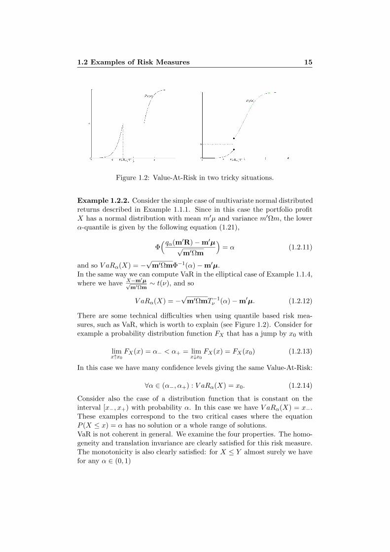
Figure 1.2: Value-At-Risk in two tricky situations.
Example 1.2.2. Consider the simple case of multivariate normal distributedreturns described in Example 1.1.1. Since in this case the portfolio profitX has a normal distribution with mean m′µ and variance m′Ωm, the lowerα-quantile is given by the following equation (1.21),
Φ(qα(m′R)−m′µ√
m′Ωm
)= α (1.2.11)
and so V aRα(X) = −√
m′ΩmΦ−1(α)−m′µ.In the same way we can compute VaR in the elliptical case of Example 1.1.4,where we have X−m′µ√
m′Ωm∼ t(ν), and so
V aRα(X) = −√
m′ΩmT−1ν (α)−m′µ. (1.2.12)
There are some technical difficulties when using quantile based risk mea-sures, such as VaR, which is worth to explain (see Figure 1.2). Consider forexample a probability distribution function FX that has a jump by x0 with
limx↑x0
FX(x) = α− < α+ = limx↓x0
FX(x) = FX(x0) (1.2.13)
In this case we have many confidence levels giving the same Value-At-Risk:
∀α ∈ (α−, α+) : V aRα(X) = x0. (1.2.14)
Consider also the case of a distribution function that is constant on theinterval [x−, x+) with probability α. In this case we have V aRα(X) = x−.These examples correspond to the two critical cases where the equationP (X ≤ x) = α has no solution or a whole range of solutions.VaR is not coherent in general. We examine the four properties. The homo-geneity and translation invariance are clearly satisfied for this risk measure.The monotonicity is also clearly satisfied: for X ≤ Y almost surely we havefor any α ∈ (0, 1)
1.2 Examples of Risk Measures 16
P [Y ≤ y] ≥ α⇒ P [X ≤ y] ≥ α (1.2.15)
and so taking the infimum it follows qα(Y ) ≥ qα(X), which implies thedesired inequality. The subadditivity property fails in general as shown bythe following simple example.
Example 1.2.3. Consider two independent payoffs X and Y with X,Y ∈[−4,−2] ∪ [1, 2] and
P (X < 0) = P (Y < 0) = 3%. (1.2.16)
For the combined position with payoff X+Y we have (because of the imageof X,Y and independence)
P (X + Y < 0) = P (X < 0, Y > 0) + P (X > 0, Y < 0)+
+ P (X < 0, Y < 0) = 5.91%(1.2.17)
and this implies q5%(X + Y ) < 0, i.e. V aR5%(X + Y ) > 0. We also haveV aR5%(X), V aR5%(Y ) ≤ 0 and so
V aR5%(X + Y ) > V aR5%(X) + V aR5%(Y ), (1.2.18)
subadditivity is thus not available.
In the literature we can find other examples of more realistic situations thanthe above where we do not have subadditivity. See for example [17] 6.7,where the authors show the lacking of subadditivity of VaR for a portfolioof defaultable bonds. Also in [8] there is a less sophisticated counterexample.Nevertheless, in the situation of elliptical distributed asset returns we havethe following result ([17] Theorem 6.8).
Theorem 1.2.1. Let R ∼ En(µ,Ω, ψ) and 0 < α ≤ 12 . Then VaR is
subadditive on M and thus coherent.
Proof. Let X1, X2 ∈ M be two portfolio profits such that X1 + X2 ∈ M.Using the definition of elliptical distributed random vectors (see AppendixA Definition A.2) we can write
X1 = m1′R = m1
′AY + m1′µ, (1.2.19)
for Y ∼ Sk(ψ), A ∈ Rn×k. By Theorem A.1
X1(d)∼ |m1
′A|Y1 + m1′µ, (1.2.20)
where |m1′A| denotes the euclidean norm of the vector m1
′A and Y1 thefirst component of Y. The translation invariance and homogeneity of VaRimply
1.2 Examples of Risk Measures 17
V aRα(X1) = |m1′A|V aRα(Y1) + m1
′µ. (1.2.21)
In the same way we have V aRα(X2) = V aRα(m2′R) = |m2
′A|V aRα(Y1) +m2′µ and V aRα(X1 +X2) = |(m1+m2)′A|V aRα(Y1)+(m1+m2)′µ. Since
Y1 is spherically distributed and must be symmetric we have V aRα(Y1) ≥ 0for α ≤ 1
2 ,
V aRα(X1 +X2) = |(m1 + m2)′A|︸ ︷︷ ︸≤|m1
′A|+|m2′A|
V aRα(Y1)︸ ︷︷ ︸≥0
+(m1 + m2)′µ
≤ V aRα(X1) + V aRα(X2).
(1.2.22)
See also [7] for more interpretation on this result. Since VaR in generaldoes not have this diversification effect, this measure may lead to unrealisticresults. An investor could for example be encouraged to split his account intotwo in order to meet the lower capital requirement. Another big issue aboutthis way of measuring the portfolio risk is that VaR provides a minimumbound for losses ignoring potential large losses beyond this limit.
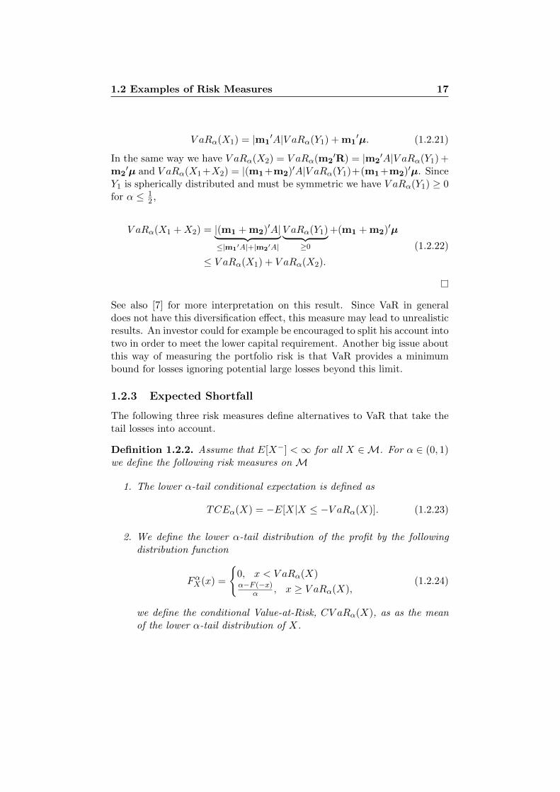
1.2.3 Expected Shortfall
The following three risk measures define alternatives to VaR that take thetail losses into account.
Definition 1.2.2. Assume that E[X−] <∞ for all X ∈M. For α ∈ (0, 1)we define the following risk measures on M
1. The lower α-tail conditional expectation is defined as
TCEα(X) = −E[X|X ≤ −V aRα(X)]. (1.2.23)
2. We define the lower α-tail distribution of the profit by the followingdistribution function
FαX(x) =
0, x < V aRα(X)α−F (−x)
α , x ≥ V aRα(X),(1.2.24)
we define the conditional Value-at-Risk, CV aRα(X), as as the meanof the lower α-tail distribution of X.
1.2 Examples of Risk Measures 18
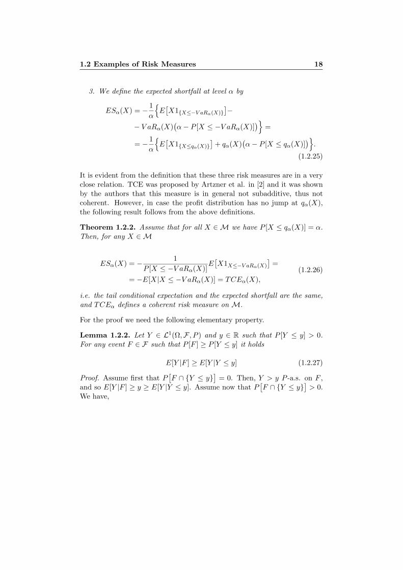
3. We define the expected shortfall at level α by
ESα(X) = − 1
α
E[X1X≤−V aRα(X)
]−
− V aRα(X)(α− P [X ≤ −V aRα(X)]
)=
= − 1
α
E[X1X≤qα(X)
]+ qα(X)
(α− P [X ≤ qα(X)]
).
(1.2.25)
It is evident from the definition that these three risk measures are in a veryclose relation. TCE was proposed by Artzner et al. in [2] and it was shownby the authors that this measure is in general not subadditive, thus notcoherent. However, in case the profit distribution has no jump at qα(X),the following result follows from the above definitions.
Theorem 1.2.2. Assume that for all X ∈ M we have P [X ≤ qα(X)] = α.Then, for any X ∈M
ESα(X) = − 1
P [X ≤ −V aRα(X)]E[X1X≤−V aRα(X)
]=
= −E[X|X ≤ −V aRα(X)] = TCEα(X),
(1.2.26)
i.e. the tail conditional expectation and the expected shortfall are the same,and TCEα defines a coherent risk measure on M.
For the proof we need the following elementary property.
Lemma 1.2.2. Let Y ∈ L1(Ω,F , P ) and y ∈ R such that P [Y ≤ y] > 0.For any event F ∈ F such that P [F ] ≥ P [Y ≤ y] it holds
E[Y |F ] ≥ E[Y |Y ≤ y] (1.2.27)
Proof. Assume first that P[F ∩ Y ≤ y
]= 0. Then, Y > y P -a.s. on F ,
and so E[Y |F ] ≥ y ≥ E[Y |Y ≤ y]. Assume now that P[F ∩ Y ≤ y
]> 0.
We have,

1.2 Examples of Risk Measures 19
E[Y |Y ≤ y] = y +1
P [Y ≤ y]
(E[(Y − y)1Y≤y∩F
]+ E
[(Y − y)1Y≤y∩(Ω\F )
]︸ ︷︷ ︸≤0
)≤ y + E
[Y − y
∣∣Y ≤ y ∩ F ]︸ ︷︷ ︸≤0
P [F |Y ≤ y]︸ ︷︷ ︸≥P [Y≤y|F ]
≤ y + E[Y − y
∣∣Y ≤ y ∩ F ]P [Y ≤ y|F ]
= y +E[(Y − y)1Y≤y∩F
]P [F ]
≤ y +E[(Y − y)1Y≤y∩F
]P [F ]
+E[(Y − y)1Y >y∩F
]P [F ]
= E[Y |F ],
(1.2.28)
which is the desired inequality.
Proof. We now prove Theorem 1.2.2. Since for any X ∈M we have P [X ≤qα(X)] = α we can immediately see that ESα(X) = TCEα(X). For thecoherence: positive homogeneity and translation invariance are clear. Forthe monotonicity consider X ≤ Y a.s.. By assumption we have P [X ≤qα(X)] = P [Y ≤ qα(Y )] = α and applying Lemma 1.2.2 we have,
ρ(X) = −E[X|X ≤ qα(X)] ≥ −E[X|Y ≤ qα(Y )]
≥ −E[Y |Y ≤ qα(Y )] = ρ(Y ).(1.2.29)
For the subadditivity applying again Lemma 1.2.2:
ρ(X + Y ) = −E[X|X + Y ≤ qα(X + Y )]− E[Y |X + Y ≤ qα(X + Y )]
≤ −E[X|X ≤ qα(X)]− E[Y |Y ≤ qα(Y )] = ρ(X) + ρ(Y ).
(1.2.30)
We defined CVaR, as in the paper [23] of Rockafellar and Uryasev, basedon a rescaled probability distribution that focus only on the lower tail partof the original distribution. From the definition above it is evident that FαXdefines a probability distribution. We represent graphically how the lowerα-tail distribution is constructed.ES generalizes TCE for the case of a jump at qα. As we are going tosee, this modification of TCE defines a coherent risk measure. In [23] theauthors discuss these definitions in details showing that CVaR and ES areactually the same. In this section we want to discuss the properties of ES

1.2 Examples of Risk Measures 20
(or CVaR). A first very useful result is the following integral representationof the expected shortfall ([1] Proposition 3.2).
Theorem 1.2.3. Assume that E[X−] <∞. Then,
ESα(X) =1
α
∫ α
0V aRu(X)du. (1.2.31)
Proof. Consider a uniformly distributed random variable on [0, 1] and definethe random variable Z = qU (X). Note that Z has the same distribution asX, since
P [Z ≤ x] = P [qU (X) ≤ x] = P [F−1X (U) ≤ x] = P [U ≤ FX(x)] = FX(x).
(1.2.32)The map u 7→ qu(X) is obviously non-decreseaing and therefore we have thefollowing sets relations
U ≤ α ⊂ qU (X) ≤ qα(X),U > α ∩ qU (X) ≤ qα(X) ⊂ qU (X) = qα(X),
(1.2.33)
which implies
U ≤ α ∪(U > α ∩ qU (X) ≤ qα(X)
)= qU (X) ≤ qα(X), (1.2.34)
where the union is disjoint. Then,∫ α
0qu(X)du = E
[qU (X)1U≤α
](1.2.32)
= E[qU (X)1qU (X)≤qα(X)
]− E
[qU (X)1U>α∩qU (X)≤qα(X)
](1.2.30)
= E[X1X≤qα(X)
]− E
[X1U>α∩X≤qα(X)
](1.2.31)
= E[X1X≤qα(X)
]− qα(X)P
[U > α ∩ X ≤ qα(X)
](1.2.32)
= E[X1X≤qα(X)
]− qα(X)
(α− P [X ≤ qα(X)]
).
(1.2.35)
Dividing both sides by −α we get the desired identity.
We now prove that the expected shortfall is a proper risk measure.
Theorem 1.2.4. Assume E[X−] < ∞ for all X ∈ M. ESα defines acoherent risk measure on M.

1.2 Examples of Risk Measures 21
Proof. 1. For λ > 0 we have
ESα(λX) = − 1
α
λE[X1X≤qα(X)
]+ λqα(X)
(α− P [λX ≤ λqα(X)]
)= λESα(X)
(1.2.36)
2. The monotonicity follows immediately by the monotonicity of VaRand the integral representation in Theorem 1.2.3.
3. Using the fact that qα(X + c) = qα(X) + c we have
ESα(X + c) = − 1
α
E[X1X≤qα(X)] + cP [X ≤ qα(X)]
+ (qα(X) + c)(α− P [X ≤ qα(X)]
)= ESα(X)− c
(1.2.37)
4. Define the following random variable
1αX≤x =
1X≤x if P [X = x] = 0,
1X≤x + α−P [X≤x]P [X=x] 1X=x if P [X = x] > 0.
(1.2.38)
This random variable satisfies
E[1αX≤qα(X)] = α. (1.2.39)
If P [X = qα(X)] > 0 then integrating (1.2.34) gives directly α. IfP [X = qα(X)] = 0 we have E[1αX≤qα(X)] = P [X ≤ qα(X)] ≥ α, on
the other hand in this case we have P [X ≤ qα(X)] = P [X < qα(X)] ≤α (see Lemma 1.2.1) and therefore the expectation must be equal toα. It also holds
E[1X≤qα(X)α ] ∈ [0, 1], (1.2.40)
this follows because P [X ≤ qα(X)] ≥ α. We have also by definition
1
αE[X1αX≤qα(X)] = −ESα(X). (1.2.41)
We also have by (1.2.36)1αZ≤qα(Z) − 1αX≤qα(X) ≥ 0 if X > qα(X),
1αZ≤qα(Z) − 1αX≤qα(X) ≤ 0 if X < qα(X),(1.2.42)
1.2 Examples of Risk Measures 22
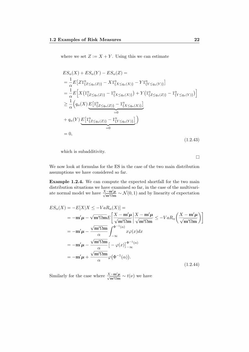
where we set Z := X + Y . Using this we can estimate
ESα(X) + ESα(Y )− ESα(Z) =
=1
αE[Z1αZ≤qα(Z) −X1αX≤qα(X) − Y 1αY≤qα(Y )
]=
1
αE[X(1αZ≤qα(Z) − 1αX≤qα(X)
)+ Y
(1αZ≤qα(Z) − 1αY≤qα(Y )
)]≥ 1
α
(qα(X)E
[1αZ≤qα(Z) − 1αX≤qα(X)
]︸ ︷︷ ︸=0
+ qα(Y )E[1αZ≤qα(Z) − 1αY≤qα(Y )
]︸ ︷︷ ︸=0
)= 0,
(1.2.43)
which is subadditivity.
We now look at formulas for the ES in the case of the two main distributionassumptions we have considered so far.
Example 1.2.4. We can compute the expected shortfall for the two maindistribution situations we have examined so far, in the case of the multivari-ate normal model we have X−m′µ√
m′Ωm∼ N (0, 1) and by linearity of expectation
ESα(X) = −E[X|X ≤ −V aRα(X)] =
= −m′µ−√
m′ΩmE
[X −m′µ√
m′Ωm
∣∣∣∣X −m′µ√m′Ωm
≤ −V aRα(X −m′µ√
m′Ωm
)]= −m′µ−
√m′Ωm
α
∫ Φ−1(α)
−∞xϕ(x)dx
= −m′µ−√
m′Ωm
α
[− ϕ(x)
]Φ−1(α)
−∞
= −m′µ +
√m′Ωm
αϕ(Φ−1(α)
).
(1.2.44)
Similarly for the case where X−m′µ√m′Ωm
∼ t(ν) we have

1.3 Euler’s Relation and Risk Contributions 23
ESα(X) = −m′µ−√
m′Ωm
α
∫ T−1ν (α)
−∞xtν(x)dx
= −m′µ−√
m′Ωm
α
[ν
1− ν
(1 +
x2
ν
)tν(x)
]T−1ν (α)
−∞
= −m′µ− ν
1− ν
√m′Ωm
α
(1 +
(T−1ν (α)
)2ν
)tν(T−1ν (α)
).
(1.2.45)
Comparing the ratio ESα(X)/V arα(X) in the two cases, it is possible toshow that in the multivariate normal model we have that
ESα(X)
V arα(X)−→ 1 (1.2.46)
as α→ 0, whereas in the elliptical model we have
ESα(X)
V arα(X)−→ ν/(ν − 1) > 1 (1.2.47)
as α → 0 (see [16] Section 4.2). The difference between VaR and ES isgreater in the elliptical case because of the heavy tails of the loss distribution.
The following characterization proved by Acerbi and Tasche in [1] allows usto think about ES as the limiting average of the worst 100α% losses. Thisresult can be used in practice to construct Monte Carlo estimates for therisk.
Lemma 1.2.3. For α ∈ (0, 1), X ∈ M with E[X−] < ∞, and (Xi)i∈N asequence of independent random variable distributed as X, we have
limn→∞
∑bnαci=1 Xi:n
bnαc= ESα(X) (1.2.48)
almost surely, where bnαc denotes the biggest integer smaller than nα andX1:n ≤ · · · ≤ Xn:n denote the components of the ordered n-tuple (X1, . . . , Xn).
1.3 Euler’s Relation and Risk Contributions
The main problem we want to focus on now is to determine the risk ofindividual securities in order to construct trading strategies that take thesingle risks of the instruments into account. It is however a quite hard taskto identify the risk of each source in large and complex portfolios. Thisis because the risk of individual securities measured by most common riskmeasures such as the ones we have discussed above do not sum up to the
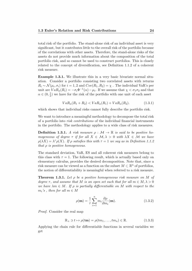
1.3 Euler’s Relation and Risk Contributions 24
total risk of the portfolio. The stand-alone risk of an individual asset is verysignificant, but it contributes little to the overall risk of the portfolio becauseof the correlations with other assets. Therefore, the stand-alone risks of theassets do not provide much information about the composition of the totalportfolio risk, and so cannot be used to construct portfolios. This is closelyrelated to the concept of diversification, see Definition 1.1.2 of a coherentrisk measure.
Example 1.3.1. We illustrate this in a very basic bivariate normal situ-ation. Consider a portfolio consisting two correlated assets with returnsRi ∼ N (µi, σi) for i = 1, 2 and Cov(R1, R2) = χ . The individual VaR’s perunit are V aRα(Ri) = −σiΦ−1(α)−µi. If we assume that χ < σ1σ2 and thatα ∈ (0, 1
2) we have for the risk of the portfolio with one unit of each asset
V aRα(R1 +R2) < V aRα(R1) + V aRα(R2). (1.3.1)
which shows that individual risks cannot fully describe the portfolio risk.
We want to introduce a meaningful methodology to decompose the total riskof a portfolio into risk contributions of the individual financial instrumentsin the portfolio. The methodology applies to a wide class of risk measures.
Definition 1.3.1. A risk measure ρ : M → R is said to be positive ho-mogeneous of degree τ if for all X ∈ M, λ > 0 with λX ∈ M we haveρ(λX) = λτρ(X). If ρ satisfies this with τ = 1 we say as in Definition 1.1.2that ρ is positive homogeneous.
The standard deviation, VaR, ES and all coherent risk measures belong tothis class with τ = 1. The following result, which is actually based only onelementary calculus, provides the desired decomposition. Note that, since arisk measure can be viewed as a function on the subset M ⊂ Rn of portfolios,the notion of differentiability is meaningful when referred to a risk measure.
Theorem 1.3.1. Let ρ be a positive homogeneous risk measure on M ofdegree τ , and assume that M is an open set such that for all m ∈M,λ > 0we have λm ∈ M . If ρ is partially differentiable on M with respect to themi’s , then for all m ∈M
ρ(m) =1
τ
n∑i=1
mi∂ρ
∂mi(m). (1.3.2)
Proof. Consider the real map
R+ 3 t 7→ ρ(tm) = ρ(tm1, . . . , tmn) ∈ R. (1.3.3)
Applying the chain rule for differentiable functions in several variables weget
1.3 Euler’s Relation and Risk Contributions 25
dρ(λm)
dλ=
n∑i=1
∂ρ(λm)
∂mimi. (1.3.4)
Because of homogeneity the left hand side becomes
dρ(λm)
dλ=
d
dλ
(λτρ(m)
)= τλτ−1ρ(m), (1.3.5)
and setting λ = 1 leads to (1.3.2).
The above decomposition is fundamental when considering risk contribu-tions and can be applied to all the risk measures seen in Section 1.2, sinceall of them are positive homogeneous measures. By quantile based risk mea-sures we need however some more assumptions on the distribution of theassets returns in order to ensure differentiability. We will discuss this aspectin details in Section 1.4. Each component mi
∂ρ(m)∂mi
, termed risk contributionof asset i, is the amount of risk contributed to the total risk by investing mi
in asset i. In the case τ = 1, the sum of all these contributions equals thetotal risk of the portfolio m. The ratio mi
ρ(m)∂ρ(m)∂mi
tells us the percentage of
total risk contributed by asset i. The term ∂ρ(m)∂mi
is referred to as marginalrisk and represents the impact on the overall risk from a small change in theposition size of asset i, keeping all other positions fixed. If the sign of themarginal risk of asset i is positive then investing a small amount of moneymore in asset i will increase the portfolio risk; and if the sign is negative wehave the opposite effect. This means that the assets with negative marginalrisk can be used as hedging instruments and for diversification. Note thatall these considerations make sense only if the increase ε in asset i is smallenough so that the incremental risk can be aproximated by
ρ(m + εei)− ρ(m) ≈ ε∂ρ(m)
∂mi, (1.3.6)
where ei denotes the canonical basis vector of Rn. For example, if the riskcontribution of asset 1, in a portfolio consisting of two assets, is twice thatof asset 2, the above relation does not imply that eliminating asset 1 fromthe portfolio will reduce the total risk by 2
3 . This is because the partialderivatives describe the risk changes only locally and both the marginalrisk and the total risk will change as the position in the asset changes. Atthis point a few questions may seem natural. Is each of the term in thedecomposition (1.3.2) really an appropriate representation of the risk con-tribution of each individual asset? If yes, is (1.3.2) the only representationthat makes sense, or are there other plausible ways of decomposing the to-tal risk? These questions have been answered by Tasche in [24]: he haspostulated a general assumption of suitability of the risk contribution, andshown that the only appropriate representation of the marginal risk is the
1.3 Euler’s Relation and Risk Contributions 26
first order partial derivative of the risk measure with respect to the positionsize. The approach by Tasche [24] is very instructive and provides intuitionabout the problem, we want therefore to discuss it. This approach is anaxiomatic one, we first define the evident properties that risk contributionsmust satisfy and then look for possible candidates. We start defining theReturn on Risk-Adjusted-Capital, a well-known concept in economy in thecontext of capital allocation,
RORAC(m) =E[m′R]
ρ(m)− E[m′R]. (1.3.7)
The RORAC of a portfolio m is defined as ration between the expected profitof the portfolio E[m′R] and the economic capital ρ(m) − E[m′R], which isthe amount of capital needed to cover the risks at some confidence level.The per-unit RORAC of asset i is given by
E[Ri]
ρ(Ri)− E[Ri], (1.3.8)
where ρ(Ri) is the risk of asset i per unit of position. The RORAC is usedto measure the performance of the portfolio: if the RORAC of portfolio Ais higher than that of portfolio B, then portfolio A gives a higher returnper unit of risk than portfolio B, and so has a better performance than Bin this terminology. Observe that the case of opposite signs in the numera-tor and denominator respectively of the RORAC is unrealistic. The case ofpositive numerator and negative economic capital means that we can investwith positive expected profit and we are even paid to do so. The oppo-site case means that we are paying for being allowed to bear someone else’srisk. Mathematically, we can describe the problem of finding risk contribu-tions as finding a vector field a = (a1, . . . , an) : M → Rn satisfying certainproperties.
Definition 1.3.2. Let ρ : M → R be a risk measure on a set of portfoliosM . A vector field a = (a1, . . . , ad) : M → Rn is said to be suitable forperformance measurement for ρ if it satisfies the following conditions.
1. For all m ∈M and i ∈ 1, . . . , n the inequality
E[Ri]
ai(m)− E[Ri]>
E[m′R]
ρ(m)− E[m′R], (1.3.9)
implies that there is an ε > 0 such that for all t ∈ (0, ε) we have
E[m′R + tRi]
ρ(m + tei)− E[m′R + tRi]>
E[m′R]
ρ(m)− E[m′R]
>E[m′R− tRi]
ρ(m− tei)− E[m′R− tRi].
(1.3.10)

1.3 Euler’s Relation and Risk Contributions 27
2. For all m ∈M and i ∈ 1, . . . , n the inequality
E[Ri]
ai(m)− E[Ri]<
E[m′R]
ρ(m)− E[m′R], (1.3.11)
implies that there is an ε > 0 such that for all t ∈ (0, ε) we have
E[m′R + tRi]
ρ(m + tei)− E[m′R + tRi]<
E[m′R]
ρ(m)− E[m′R]
<E[m′R− tRi]
ρ(m− tei)− E[m′R− tRi].
(1.3.12)
To better understand why 1 and 2 are two universal properties that the riskcontributions must satisfy in order to be coherent with their interpretation,we explain the meaning of the above conditions. The inequality (1.3.9) tellsus that the performance of one unit of the asset i as part of the portfoliois higher than that of the entire portfolio. If such a relation holds, the in-equalities (1.3.10) tells us that investing a little more (less) in asset i shouldincrease (decrease) the performance of the entire portfolio. The inequalities(1.3.11) and (1.3.12) are the corresponding ones with reverted inequalitysigns. Note that the initial risk measure ρ(Ri) in the per-unit individualRORAC of asset i is replaced by ai(m), the candidate for the risk contri-bution measure of asset i in the portfolio. Tasche [24] shows that undercertain assumptions the only candidate for the risk contribution vector fieldsatisfying the above suitability properties based on RORAC is the vector ofthe partial derivatives. Here the result exposed formally.
Theorem 1.3.2. Let ρ : M → R be a partially differentiable risk measureon an open set of portfolios M with continuous partial derivatives. Leta = (a1, . . . , an) : M → Rn be a continuous vector field. Then a is suitablefor performance measurement with ρ if and only if
ai(m) =∂ρ
∂mi(m), for all i = 1, . . . , n, m ∈M (1.3.13)
Proof. We explain the argument proposed by Tasche [24]. For m ∈M withρ(m) 6= E[m′R], and i = 1, . . . , n it holds
∂RORAC(m)
∂mi=
1(ρ(m)− E[m′R]
)2(ρ(m)E[Ri]−∂ρ
∂miE[m′R]
)=
1(ρ(m)− E[m′R]
)2(ρ(m)E[Ri]− ai(m)E[m′R]
+(ai(m)− ∂ρ
∂mi(m)
)E[m′R]
).
(1.3.14)
1.3 Euler’s Relation and Risk Contributions 28
If (1.3.13) is satisfied then for any i = 1, . . . , n condition 1 (or 2) in Definition
1.3.2 implies ∂RORAC(m)∂mi
> 0(< 0) and therefore (1.3.10) and (1.3.12) aresatisfied. For the other direction fix any i = 1, . . . , n and note that bycontinuity we only need to show (1.3.13) for m ∈ M such that mi 6= 0 andmj 6= 0 for some j 6= i. We consider separately the following cases.
1. ai(m) 6= 0, ρ(m) 6= 0, ρ(m) 6= miai(m).
2. ai(m) 6= 0, ρ(m) 6= 0, ρ(m) = miai(m).
3. ai(m) = 0, ρ(m) 6= 0.
4. ρ(m) = 0, each neighborhood of m contains some q such that ρ(q) 6= 0.
5. ρ(q) = 0, for all q is some neighborhood of m.
Note that 5 is clear since in this case ρ = 0 and ∂RORAC(m)∂mi
= 0 in someneighborhood of m, and 4 follows by continuity once we have proved thestatement in the other three cases. For case 1 choose the returns R(t) suchthat
E[Rk(t)] =
1 k = itmj
(ρ(m)ai(m) −mi
)k = j
0 k 6= i, j
(1.3.15)
for t ∈ (0, 1). For these expected returns we have
m′E[R(t)] = tρ(m)
ai(m)+ (1− t)mi
E[Ri(t)]ρ(m)− ai(m)m′E[R(t)] = (1− t)(ρ(m)−miai(m)).
(1.3.16)
Thus, it is possible to choose two sequences (tk), (sk) with tk, sk → 1, suchthat m′E[R(sk)] 6= ρ(m) 6= m′E[R(tk)], (tk) satisfies (1.3.9) and (sk) satis-fies (1.3.11). By suitableness and (1.3.14) we have
(1− tk)(ρ(m)−miai(m))
+(ai(m)− ∂ρ
∂mi(m)
)(tkρ(m)
ai(m)+ (1− tk)mi
)≥ 0,
(1− sk)(ρ(m)−miai(m))
+(ai(m)− ∂ρ
∂mi(m)
)(skρ(m)
ai(m)+ (1− sk)mi
)≤ 0.
(1.3.17)
Now k →∞ yields (1.3.13). For case 2 or 3 proceed analogously.
1.4 Differentiating Risk Measures 29
The main limitation of this approach is the use of RORAC for performancemeasurement, which is appropriate for banks, but not necessarily in everyfinancial context, thus the above argument may not be valid in general.However, the use of the partial derivatives can be justified by the fact thatit describes how the total risk of the portfolio changes if there is a small localchange in one of the positions. Another justification, based on the notion of”fairness” in cooperative game theory, was given by Denault [5].
1.4 Differentiating Risk Measures
Considering the above discussion we are now interested in examining if themost common risk measures can be differentiated and in computing thesepartial derivatives. We also want to see if under the most common dis-tribution assumptions for the portfolio returns we can explicitly find thesederivatives. This is interesting because we would like to use the informationgiven by the risk contributions to construct risk-balanced portfolios. Wetreat systematically the differentiation of the risk measures considered inSection 1.2.
1.4.1 Derivatives of the Standard Deviation and CovarianceBased Risk Contributions
For m ∈M ⊂ Rn we have
ρ(m) =√
m′Ωm, (1.4.1)
where we use the same notation as in (1.2.2). The partial derivatives aregiven by
∂ρ(m)
∂mk=
1
2√
m′Ωm
∂
∂mk
( n∑i=1
n∑j=1
mimjΩij
)
=1√
m′Ωm
n∑j=1
mjΩkj
=1√
m′Ωm(Ωm)k.
(1.4.2)
The risk contributions are therefore given by
mi√m′Ωm
(Ωm)i, i = 1, . . . , d (1.4.3)
and depend only on the covariances Cov(Ri, Rj) for i 6= j and variancesV ar[Ri] of the asset returns. The problem of estimating these parameters
1.4 Differentiating Risk Measures 30
will be considered later. The decomposition of the homogeneous measure σcan be written as
σ(m) =1
σ(m)
n∑i=1
mie′iΩm, (1.4.4)
where ei is the standard basis vector in Rn. We now want to comparethe risk contributions obtained with partial derivatives with the covariancebased risk contributions widely used in practice. The covariance based riskcontributions are obtained using the notion of best linear predictor for ran-dom variables in L2.
Definition 1.4.1. Let Y, Z be two square integrable random variables sothat V ar[Z] > 0. For z ∈ R we define the projection πZ(z, Y ) of Y − E[Y ]onto the linear space spanned by Z − E[Z] via
πZ(z, Y ) =Cov(Y,Z)
V ar[Z]z. (1.4.5)
The function πZ(z, Y ) is the best linear predictor of Y − E[Y ] given Z −E[Z] = z in the sense that the random variable πZ
(Z −E[Z], Y
)minimizes
the L2-distance between Y −E[Y ] and the linear space spanned by Z−E[Z].Indeed, for θ ∈ R,
E[(
(Y − E[Y ])− θ(Z − E[Z]))2]
= V ar[Y − θZ] =
= V ar[Y ]− 2θCov(Y, Z) + θ2V ar[Z](1.4.6)
and minimizing over θ shows the statement. This has been applied in thecontext of risk contributions in the following way: we define the set of port-folios M ⊂ Rn as
M :=m ∈ Rn : V ar[m′R] > 0
, (1.4.7)
and note that for any m ∈ M , λ > 0 it holds λm ∈ M . The idea ofthis method is to set Z := m′R, Y := miRi and choose a value for z =m′R − E[m′R] corresponding to a worst-case scenario and use the bestlinear predictor to determine the risk contribution. We set z = ρ(m) to bethe portfolio risk. The vector field of risk contributions obtained with thismethod is then defined by
ai(m) := πm′R(ρ(m),miRi
)=Cov(miRi,m
′R)
V ar[m′R]ρ(m)
=mi∑n
j=1mjCov(Ri, Rj)
V ar[m′R]ρ(m) =
mi(Ωm)im′Ωm
ρ(m),
(1.4.8)
1.4 Differentiating Risk Measures 31
where Ω denotes the covariance matrix of R. We interpret the so constructedai(m) as the best linear predictor of the profit fluctuation of asset i giventhat the portfolio profit fluctuation is just the risk ρ(m). For the standarddeviation ρ(m) = σ(m) we get
ai(m) =mi(Ωm)i√
m′Ωm= mi
∂σ(m)
∂mi, (1.4.9)
i.e. in this case we have the same risk contribution as the ones obtained withpartial derivatives and since σ : M → R is homogenous we can decomposethe total risk in the risk contributions as in (1.3.2). However, we are goingto see that for other risk measures the ai’s obtained using the best linearpredictor can differ considerably from the partial derivatives and should notbe used for risk contributions measurements even if
ρ(m) =
n∑i=1
miai(m) (1.4.10)
still holds.
1.4.2 Derivatives of the Value-At-Risk
We have a closer look at the problem of differentiating VaR, although, asexplained in Section 1.2, VaR represents a problematic risk measure. Thisis anyway interesting because we are going to deal with the problem ofdifferentiating the lower α-quintile of the profit distribution, which is rel-evant also when considering the expected shortfall derivatives. In generalthe quantile function qα(m) is not differentiable in m. In order to guaranteethe existence of the partial derivatives we need to impose some technicalassumptions on the distribution of the random vector R = (R1, . . . , Rn).Tasche [25] discusses this problem in mathematical details. We expose theessential theoretical aspects treated in [25]. We begin recalling a basic defi-nition from probability theory.
Definition 1.4.2. For the random vector R = (R1, . . . , Rn), R1 is saidto have a conditional density given (R2, . . . , Rn) if it exists a measurablefunction γ : Rn → [0,∞) such that for all A ∈ B(R)
P [R1 ∈ A|R2, . . . , Rn] =
∫Aγ(t, R2, . . . , Rn)dt. (1.4.11)
Note that the existence of a joint density of R implies the existence ofa conditional density but not necessarily vice versa. Very useful for thecomputation of the quantile derivatives is the following result.
Lemma 1.4.1. Assume that R1 has a conditional density given (R2, . . . , Rn).Then for any portfolio m with m1 6= 0 we have
1.4 Differentiating Risk Measures 32
1. The random variable X = m′R has a density given by
fX(x) =1
|m1|E[γ(x−∑n
i=2miRim1
, R2, . . . , Rn
)]. (1.4.12)
2. If fX(x) > 0 we have for i = 2, . . . , n,
E[Ri|X = x] =
E
[Riγ
(1m1
(x−
∑nj=2mjRj
), R2, . . . , Rn
)]E
[γ(
1m1
(x−
∑nj=2mjRj
), R2, . . . , Rn
)] .
(1.4.13)
3. If fX(x) > 0 we have
E[R1|X = x] =
E
[x−
∑nj=2mjRjm1
γ(
1m1
(x−
∑nj=2mjRj
), R2, . . . , Rn
)]E
[γ(
1m1
(x−
∑nj=2mjRj
), R2, . . . , Rn
)] .
(1.4.14)
Proof. 1. Consider m1 > 0 (for m1 < 0 proceed analogue), using theproperty of conditional expectations we have
P [X ≤ x] = E[1X≤x] = E[E[1X≤x|R2, . . . , Rn]
]= E
[E[1R1≤m−1
1 (x−∑ni=2miRi)
|R2, . . . , Rn]]
= E
[ ∫ m−11 (x−
∑ni=2miRi)
−∞γ(u,R2, . . . , Rn)du
]= E
[ ∫ x
−∞
1
m1γ(u−∑n
i=2miRim1
, R2, . . . , Rn
)du
]=
∫ x
−∞E
[1
m1γ(u−∑n
i=2miRim1
, R2, . . . , Rn
)]du,
(1.4.15)
where in the last step we have exchanged the order of integration,which is allowed by Fubini’s theorem. Therefore the density of X isgiven by the integrand in the right hand side.
2. Provided that fX(x) > 0 we can write
E[Ri|X = x] =E[Ri1X=x]
P [X = x]= lim
δ↓0
δ−1E[Ri1x<X≤x+δ]
δ−1P (x < X ≤ x+ δ)
=∂∂xE[Ri1X≤x]
fX(x).
(1.4.16)
1.4 Differentiating Risk Measures 33
Note that exchanging the limit and the expectation can be justifiedby dominated convergence. The denominator was calculated in 1 andthe numerator can be computed as in 1, for m1 > 0 and i = 2, . . . , n,
∂E[Ri1X≤x]
∂x=
∂
∂xE[E[Ri1X≤x|R2, . . . , Rn]
]=
=∂
∂xE[RiE[1X≤x|R2, . . . , Rn]
]=
=∂
∂xE
[Ri
∫ x
−∞
1
m1γ(u−∑n
i=2miRim1
, R2, . . . , Rn
)du
]=
=1
m1E[Riγ
(x−∑ni=2miRim1
, R2, . . . , Rn
)],
(1.4.17)
where we have exchanged again integration w.r.t. u and expectation,and then taken the derivative with respect to x. The identity 2 followsform 1 and the last equality.
3. We can write
E[R1|X = x] = E
[x−
∑nj=2mjRj
m1
∣∣∣∣X = x
], (1.4.18)
and applying 2 we get 3.
The quantities determined in the above result motivate the following as-sumptions on γ made by Tasche in [25].
Assumptions 1.4. Let the conditional density γ satisfy the following as-sumptions.
1. For fixed r2, . . . , rn the map t 7→ γ(t, r2, . . . , rn) is continuous in t.
2. The map (t,m) 7→ E[γ(x−
∑ni=2miRim1
, R2, . . . , Rn
)]is finite valued and
continuous.
3. For i = 2, . . . , n the map (t,m) 7→ E[Riγ
(x−
∑ni=2miRim1
, R2, . . . , Rn
)]is finite valued and continuous.
Typical situations where these assumptions are satisfied are listed by Tasche[25] in Remark 2.4. Tasche [25] gives in Lemma 3.2 and Theorem 3.3 rigor-ous mathematical arguments, using the implicit function theorem, showingthat if the above assumptions are satisfied then the quantile function qαis partially differentiable. Once we know that qα is differentiable with re-spect to the components of m we can obtain representations of the partialderivatives in terms of expectations of conditional distributions by applyingLemma 1.4.1.
1.4 Differentiating Risk Measures 34
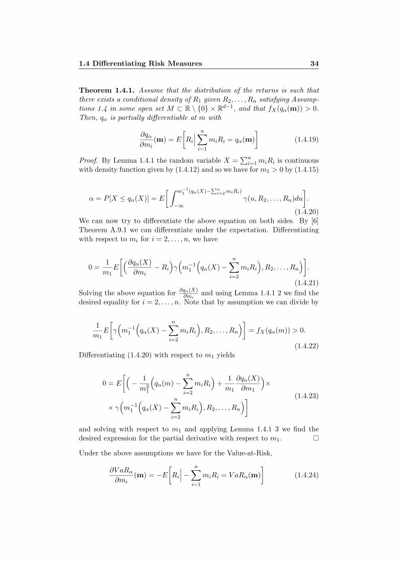
Theorem 1.4.1. Assume that the distribution of the returns is such thatthere exists a conditional density of R1 given R2, . . . , Rn satisfying Assump-tions 1.4 in some open set M ⊂ R \ 0 × Rd−1, and that fX(qα(m)) > 0.Then, qα is partially differentiable at m with
∂qα∂mi
(m) = E
[Ri
∣∣∣ n∑i=1
miRi = qα(m)
](1.4.19)
Proof. By Lemma 1.4.1 the random variable X =∑n
i=1miRi is continuouswith density function given by (1.4.12) and so we have for m1 > 0 by (1.4.15)
α = P [X ≤ qα(X)] = E
[ ∫ m−11 (qα(X)−
∑ni=2miRi)
−∞γ(u,R2, . . . , Rn)du
].
(1.4.20)We can now try to differentiate the above equation on both sides. By [6]Theorem A.9.1 we can differentiate under the expectation. Differentiatingwith respect to mi for i = 2, . . . , n, we have
0 =1
m1E
[(∂qα(X)
∂mi−Ri
)γ(m−1
1
(qα(X)−
n∑i=2
miRi
), R2, . . . , Rn
)].
(1.4.21)
Solving the above equation for ∂qα(X)∂mi
and using Lemma 1.4.1 2 we find thedesired equality for i = 2, . . . , n. Note that by assumption we can divide by
1
m1E
[γ(m−1
1
(qα(X)−
n∑i=2
miRi
), R2, . . . , Rn
)]= fX(qα(m)) > 0.
(1.4.22)Differentiating (1.4.20) with respect to m1 yields
0 = E
[(− 1
m21
(qα(m)−
n∑i=2
miRi
)+
1
m1
∂qα(X)
∂m1
)×
× γ(m−1
1
(qα(X)−
n∑i=2
miRi
), R2, . . . , Rn
)] (1.4.23)
and solving with respect to m1 and applying Lemma 1.4.1 3 we find thedesired expression for the partial derivative with respect to m1.
Under the above assumptions we have for the Value-at-Risk,
∂V aRα∂mi
(m) = −E[Ri
∣∣∣− n∑i=1
miRi = V aRα(m)
](1.4.24)

1.4 Differentiating Risk Measures 35
and the risk decomposition into individual risk contributions is given by,
V aRα(m) = −n∑i=1
miE[Ri
∣∣∣−X = V aRα(m)]. (1.4.25)
We consider again the simple situations of Examples 1.1.1 and 1.1.4.
Example 1.4.1. Using the explicit formulas of VaR given in Example 1.2.2we can compute the partial derivatives. For the multivariate normal model,
∂V aRα∂mi
(m) = − (Ωm)i√m′Ωm
Φ−1(α)− µi, (1.4.26)
and for the elliptical model of 1.1.4
∂V aRα∂mi
(m) = − (Ωm)i√m′Ωm
T−1ν (α)− µi. (1.4.27)
The Euler decomposition of the positive homogeneous measure VaR is thengiven by
V aRα(m) =n∑i=1
mi
(− (Ωm)i√
m′ΩmΦ−1(α)− µi
). (1.4.28)
and analogously for the other model. We can observe that the risk contribu-tions obtained by differentiating VaR differ from the ones obtained by thebest linear predictor:
mi(Ωm)im′Ωm
V aRα(m) = −mi(Ωm)i√m′Ωm
Φ−1(α)− mi(Ωm)im′Ωm
m′µ. (1.4.29)
1.4.3 Derivatives of the Expected Shortfall
Once we have done all the work of Section 1.4.2 considering the partialderivatives of the lower quantile function, it is quite clear how to find ana-logue representations of the partial derivatives for the expected shortfall.
Theorem 1.4.2. Assume that the distribution of R satisfies the assump-tions of Theorem 1.4.1. Then the risk measure ESα is partially differentiablewith partial derivatives given by
∂ESα(X)
∂mi= − 1
α
E[Ri1X≤qα(X)
]+E[Ri|X = qα(X)
](α−P [X ≤ qα(X)]
)(1.4.30)
for any X ∈M with E[X−] <∞.
1.4 Differentiating Risk Measures 36
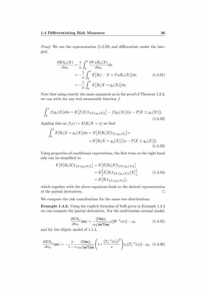
Proof. We use the representation (1.2.29) and differentiate under the inte-gral,
∂ESα(X)
∂mi=
1
α
∫ α
0
∂V aRu(X)
∂midu
= − 1
α
∫ α
0E[Ri| −X = V aRu(X)
]du
= − 1
α
∫ α
0E[Ri|X = qu(X)
]du.
(1.4.31)
Note that using exactly the same argument as in the proof of Theorem 1.2.3,we can write for any real measurable function f
∫ α
0f(qu(X))du = E
[f(X)1X≤qα(X)
]− f(qα(X))
(α− P [X ≤ qα(X)]
).
(1.4.32)Appling this on f(x) := E[Ri|X = x] we find∫ α
0E[Ri|X = qu(X)]du = E
[E[Ri|X]1X≤qα(X)
]+
+ E[Ri|X = qα(X)
](α− P [X ≤ qα(X)]
).
(1.4.33)
Using properties of conditional expectations, the first term on the right handside can be simplified to
E[E[Ri|X]1X≤qα(X)
]= E
[E[Ri|X]1X≤qα(X)
]= E
[E[Ri1X≤qα(X)
∣∣X]]= E
[Ri1X≤qα(X)
],
(1.4.34)
which together with the above equations leads to the desired representationof the partial derivatives.
We compute the risk contributions for the same two distributions.
Example 1.4.2. Using the explicit formulas of VaR given in Example 1.2.4we can compute the partial derivatives. For the multivariate normal model,
∂ESα∂mi
(m) =(Ωm)i
α√
m′Ωmϕ(Φ−1(α)
)− µi (1.4.35)
and for the elliptic model of 1.1.4,
∂ESα∂mi
(m) = − ν
1− ν(Ωm)i
α√
m′Ωm
(1+
(T−1ν (α)
)2ν
)tν(T−1ν (α)
)−µi. (1.4.36)
1.4 Differentiating Risk Measures 37
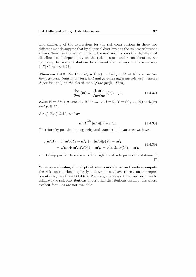
The similarity of the expressions for the risk contributions in these twodifferent models suggest that by elliptical distributions the risk contributionsalways ”look like the same”. In fact, the next result shows that by ellipticaldistributions, independently on the risk measure under consideration, wecan compute risk contributions by differentiation always in the same way([17] Corollary 6.27)
Theorem 1.4.3. Let R ∼ En(µ,Ω, ψ) and let ρ : M → R be a positivehomogeneous, translation invariant and partially differentiable risk measuredepending only on the distribution of the profit. Then,
∂ρ
∂mi(m) =
(Ωm)i√m′Ωm
ρ(Y1)− µi, (1.4.37)
where R = AY +µ with A ∈ Rn×k s.t. A′A = Ω, Y = (Y1, . . . , Yk) ∼ Sk(ψ)and µ ∈ Rn.
Proof. By (1.2.19) we have
m′R(d)∼ |m′A|Y1 + m′µ. (1.4.38)
Therefore by positive homogeneity and translation invariance we have
ρ(m′R) = ρ(|m′A|Y1 + m′µ) = |m′A|ρ(Y1)−m′µ
=√
m′A(m′A)′ρ(Y1)−m′µ =√
m′Ωmρ(Y1)−m′µ,(1.4.39)
and taking partial derivatives of the right hand side proves the statement.
When we are dealing with elliptical returns models we can therefore computethe risk contributions explicitly and we do not have to rely on the repre-sentations (1.4.24) and (1.4.30). We are going to use these two formulas toestimate the risk contributions under other distributions assumptions whereexplicit formulas are not available.

Chapter 2
Portfolio Construction
2.1 Classical Methods and Risk Contributions
We begin this chapter with a brief outline of the classical portfolio selectiontheory and discuss the drawbacks in practical applications of the classicalsolutions. The aim of this section is not to discuss every aspect of the clas-sical portfolio theory in detail, but rather to motivate the necessity of a newapproach that takes into account the risk contributions we have introducedin the previous chapter. A complete description of the classical portfolio se-lection theory can be found in [18] Chapter 6 and [10]. We now introduce afew additional notation in order to formulate the selection problem in termsof portfolio weights. We fix a certain initial wealth C > 0 the investor wantsto allocate in the n investment opportunities. For a certain portfolio m wedefine the vector of portfolio weights w = (w1, . . . , wn) by
wi =mi
C, (2.1.1)
for i = 1 . . . , n. The i-th component of this vector represents the fraction ofthe initial capital invested in instrument i. In this way, we can represent aportfolio with a vector w ∈ Rn of portfolio weights and a set of admissibleportfolios with a corresponding set of portfolio weights W . Using this nota-tion the portfolio return is given by w′R. Typical constraints on the set ofadmissible strategies are
1. W+1 = w ∈ [0, 1]n : 1′w = 1
2. W+l = w ∈ Rn+ : 1′w = l for a certain leverage l ≥ 1.
3. Wl = w ∈ Rn : 1′w = l for a certain l ≥ 1.
In the first case we do not allow borrowing of additional capital to invest orshort selling of instruments. In the second case we can borrow additionalcapital at leverage l, in the third one, borrowing and short-selling are both

2.1 Classical Methods and Risk Contributions 39
allowed. It is convenient for notational purposes when considering the prob-lem of portfolio selection to characterize strategies using weights instead ofamounts of money as we did in Chapter 1. Fix now a certain initial wealthC > 0 and a certain set of admissible strategies W . Let ρ be a partiallydifferentiable positive homogenous risk measure defined on an open set thatcontains all vectors of the form λw for w ∈W and λ > 0 (cone). In this set-ting the portfolio risk is proportional to the quantity ρ(w) = ρ(w′R), whichis the risk of the portfolio return and can be interpreted as the portfoliorisk per unit of initial capital invested. The problem of portfolio selectionconsists in formulating a criterion to select an optimal investment strategyw∗ ∈ W . A well-known method is the mean-ρ approach, that consists inminimizing the portfolio risk, under a fixed expected portfolio return, overall admissible strategies. Precisely, we select the optimal strategy as follows.
Definition 2.1.1. The mean-ρ optimal portfolio w∗ ∈ W for a certainexpected return µ∗ ∈ E[w′R] : w ∈W is defined by
w∗ = arg minw∈Wρ(w) under the constraint E[w′R] = µ∗. (2.1.2)
This approach has been proposed by Markowitz in [14] and [15] more thanfifty years ago using the variance ρ(w) = σ2(w) = w′Ωw as risk measure.Markowitz approach is also referred to in the literature as mean-varianceapproach. In case of elliptical distributed return vector R, there is howeverno difference between minimizing the risk under any positive homogenoustranslation invariant risk measure and minimizing under the variance. Pre-cisely we have the following result from [17] Proposition 6.13.
Theorem 2.1.1. Let R ∼ En(µ,Ω, ψ) with V ar[Ri] < ∞ for all i =1, . . . , n. Assume that ρ is also translation invariant and depends only onthe distribution of the profit. Then,
arg minw∈W,E[w′R]=µ∗ρ(w) = arg minw∈W,E[w′R]=µ∗w′Ωw. (2.1.3)
Proof. Recall (1.2.19),
w′R(d)∼ w′ΩwY1 + w′µ, (2.1.4)
form which it follows that for every portfolio w ∈W with E[w′R] = µ∗ wehave
ρ(w′R) = ρ(w′Ωw + µ∗
)= w′Ωwρ(Y1)− µ∗, (2.1.5)
which implies the statement.
The mean-variance approach by Markowitz appears very powerful and ele-gant. Even if for general constraints there is no analytical solution for the

2.1 Classical Methods and Risk Contributions 40
minimization problem, the quadratic programming method of numerical op-timization can be be applied to minimize efficiently the quadratic functionw′Ωw under linear constraints (see [21] Chapter 16). Despite these appeal-ing features, this approach involves several difficulties when applied in prac-tice. First of all, the output of the optimization problem is very sensitive tochanges in the input parameters. It has been observed, see for example [4],that small variations in estimating the expected returns of the instrumentscan lead to significantly different strategies. Secondly, the mean-ρ optimalportfolios optimize only the overall risk of the portfolio, without using anyinformation about how the single instruments contribute to the total risk.This leads to poor risk diversified strategies. In fact, it has been observedthat these portfolios tend to be concentrated in a very limited subset of allthe instruments. The criterion of selection of Definition 2.1.1 can lead torisky non-diversified portfolios in situations where the risk measure ρ is notcoherent. We consider VaR in the case of Example 1.1.3 (from [17] Example6.12)
Example 2.1.1. Consider portfolios w ∈ W+1 of n defaultable bonds such
as in Example 1.1.3. We assume additionally that the individual returns anddefault probabilities are all the same and equal to r = 0.05 and p = 0.03respectively. The portfolio return is then given by
w′R = (1 + r)n∑i=1
wiIi − 1, (2.1.6)
and the expected portfolio return, which is given by r(1 − p) − p, is inde-pendent of the chosen strategy w. The mean-VaR optimal portfolio at levelα = 0.05 is therefore given by
arg minw∈W+1V aRα(w′I), (2.1.7)
where I = (I1, . . . , In). Since for any strategy w ∈W+1 it holds w′I ≤ 1, we
have that V aRα(w′I) ≥ −1. The lower bound can be achieved by investingall the money in one bond and taking no positions in the others. Thisstrategy, where we set w1 = 1 and w2 = · · · = wn = 0, is therefore a mean-VaR optimal strategy, but our intuition about risk tells us that splitting ourmoney in many bonds should be less risky. This happens because we arein a situation where Value-at-Risk is not subadditive, and so it does notrepresent the diversification effect. This is of course a simplistic situationbut similar effects can be observed also in real-world settings. Better mean-ρportfolios in this situation can be obtained by replacing V aR with a coherentrisk measure such as ES.
Another well-known simple solution is the so called minimum variance port-folio, abbreviated MV portfolio,
2.1 Classical Methods and Risk Contributions 41
wmv = arg minw∈Ww′Ωw, (2.1.8)
where we minimize without imposing any condition on the overall portfolioreturn. This appears more robust than the mean-variance framework sincewe do not need to estimate the expected returns. Nevertheless, these port-folios still suffer from poor risk diversification. In the case W+
l for a certainleverage l ≥ 1, a very heuristic approach is given by the so called equallyweighted portfolio, abbreviated 1
n -portfolio, where we simply set
wi =l
n. (2.1.9)
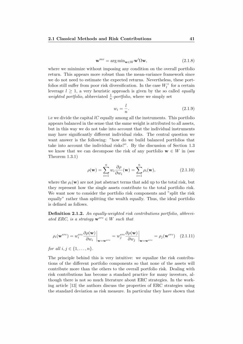
i.e we divide the capital lC equally among all the instruments. This portfolioappears balanced in the sense that the same weight is attributed to all assets,but in this way we do not take into account that the individual instrumentsmay have significantly different individual risks. The central question wewant answer is the following: ”how do we build balanced portfolios thattake into account the individual risks?”. By the discussion of Section 1.3we know that we can decompose the risk of any portfolio w ∈ W in (seeTheorem 1.3.1)
ρ(w) =
n∑i=1
wi∂ρ
∂wi(w) =
n∑i=1
ρi(w), (2.1.10)
where the ρi(w) are not just abstract terms that add up to the total risk, butthey represent how the single assets contribute to the total portfolio risk.We want now to consider the portfolio risk components and ”split the riskequally” rather than splitting the wealth equally. Thus, the ideal portfoliois defined as follows.
Definition 2.1.2. An equally-weighted risk contributions portfolio, abbrevi-ated ERC, is a strategy werc ∈W such that
ρi(werc) = werci
∂ρ(w)
∂wi
∣∣∣∣w=werc
= wercj∂ρ(w)
∂wj
∣∣∣∣w=werc
= ρj(werc) (2.1.11)
for all i, j ∈ 1, . . . , n.
The principle behind this is very intuitive: we equalize the risk contribu-tions of the different portfolio components so that none of the assets willcontribute more than the others to the overall portfolio risk. Dealing withrisk contributions has become a standard practice for many investors, al-though there is not so much literature about ERC strategies. In the work-ing article [13] the authors discuss the properties of ERC strategies usingthe standard deviation as risk measure. In particular they have shown that
2.2 ERC Strategies using Standard Deviation 42
ERC portfolios are located between the mean-variance strategies and theequally-weighted strategies in terms of volatility. There isn’t however as faras we know any literature where other risk measures are considered. Pro-vided that the risk measures satisfy the necessary assumptions there are notheoretical difficulties in applying the ERC principle on VaR, ES or otherrisk measures. Especially in the case of elliptical distributions, where byTheorem 1.4.3, the risk contributions can be computed explicitly and arevery similar to the ones of the standard deviation. In the next section weconsider ERC strategies from analytical and numerical point of view usingthe standard deviation risk measure. We will follow quite closely the workdone in the paper [13]. We will then explain how the problem of findingERC strategies looks like when other risk measures are considered.
2.2 ERC Strategies using Standard Deviation
2.2.1 The Problem
Assume that V ar[Ri] < ∞ for all i = 1, . . . , n. Let Ω as in Section 1.2 de-notes the positive definite covariance matrix of R and consider the standarddeviation risk measure σ(w) =
√w′Ωw, which is a positive homogenous
partially differentiable risk measure defined on the whole Euclidean spaceRn. Let, as in the previous section, C > 0 and W ⊂ Rn be a fixed initialwealth and a fixed set of admissible strategies. We will often restrict our-selves to the case of W+
l , mentioning explicitly when doing so. Recallingequation (1.4.3), the risk contributions for the standard deviation are givenby
ρi(w) = wi
∑j 6=iwjχijσiσj + σ2
iwi
σ(w), (2.2.1)
where we use the notation σ2i = V ar[Ri] and χij =
Cov(Ri,Rj)σiσj
. We look
therefore for a portfolios werc such that
werci∑k 6=i
werck χikσiσk + σ2iw
erci = wercj
∑k 6=j
werck χjkσjσk + σ2jw
ercj (2.2.2)
for all i, j = 1, . . . , n. Equation (2.2.2) can be written more compactly aswerci
(Ωwerc
)i
= wercj(Ωwerc
)j. If such a strategy exists is not immediately
clear from the equations and the existence depends on the constraints. Wewill show that for the case of W+
l the ERC portfolio exists and is unique.If the ERC portfolio werc ∈W exists, it means that there exists a constantc > 0 such that
werc ⊗ Ωwerc = c1, (2.2.3)
2.2 ERC Strategies using Standard Deviation 43
where ⊗ denotes the element by element product. To develop some intuitionabout how the ERC strategy is selected we consider the following example.
Example 2.2.1. For the case of W+l , we rewrite equation (2.2.2) in a nicer
way. Define,
βi(w) =1
σ(w)Cov
(Ri,
n∑k=1
wkRk
)=
∑k 6=iwkχikσiσk + σ2
iwi
σ(w), (2.2.4)
and thus ρi(w) = wiβi(w). The condition ρi(w) = ρj(w) is thus equivalentto wiβi(w) = wjβj(w) for all i, j. Using the constraint that the portfolioweights add up to l, the ERC condition can then be equivalently reformu-lated in the following way.
n∑j=1
wj = l⇔n∑j=1
βi(w)wj = βi(w)l⇔n∑j=1
βi(w)βi(w)wiβj(w)
= βi(w)l
⇔ wi =βi(w)−1l∑nj=1 βj(w)−1
,
(2.2.5)
by definition of the ERC strategy we have ρi(w)σ(w) = 1
n , thus
n∑j=1
βj(w)−1 =n∑j=1
wjσ(w)
ρj(w)= n
n∑j=1
wj = nl, (2.2.6)
and therefore (2.2.2) is equivalent to the equations
wi =1
nβi(w)(2.2.7)
for i = 1, . . . , n. We can observe that the higher (lower) is the beta ofthe asset i, the lower (higher) is the proportion invested in i. This meansthat we dislike components with high volatility or high correlations withother assets. Note that the constraint
∑ni=1wi = l is only a normalizing
one. Given any solution in w ∈ W+ we can find an ERC strategy in W+l
dividing the previous solution by l1′w .
A general closed-form solution for the ERC strategy is not available, butin some very simple situations it is possible to compute the ERC portfoliosexplicitly.
Example 2.2.2. Consider a two asset case with constraints W+1 . The co-
variance matrix is given by

2.2 ERC Strategies using Standard Deviation 44
Ω =
[σ2
1 χσ1σ2
χσ1σ2 σ22
], (2.2.8)
where σ1, σ2 are the individual return standard deviations and χ denotes thecorrelation coefficient of R1 and R2. We look for a portfolio w = (w, 1−w)such that σ1(w, 1− w) = σ2(w, 1− w). For the partial derivatives we have
∇wσ(w, 1− w) =(wσ2
1 + (1− w)χσ1σ2, (1− w)σ22 + wχσ1σ2)√
w2σ21 + 2χσ1σ2w(1− w) + (1− w)2σ2
2
, (2.2.9)
and therefore the ERC portfolio must satisfy the following quadratic equa-tion,
(σ21 − σ2
2)w2 + 2σ22w − σ2
2 = 0, (2.2.10)
with solutions given by
w(1) =σ2
σ1 + σ2, w(2) =
σ2
σ2 − σ1. (2.2.11)
the first solution is acceptable since both w(1) and 1−w(1) lie in the interval[0, 1]. For w(2) to be acceptable we need σ2 > σ1 but in this case for theother component of the portfolio we have,
1− w(2) = − σ1
σ2 − σ1< 0, (2.2.12)
and so the second solution of the quadratic equation does not lead to anERC portfolio satisfying the desired constraints. Thus, we have a uniqueERC portfolio for these constraints given by
werc =( σ2
σ1 + σ2,
σ1
σ1 + σ2
). (2.2.13)
Example 2.2.3. Let us consider a portfolio of n financial instruments forwhich we assume that
Cov(Ri, Rj) = χσiσj , (2.2.14)
for all i 6= j, i.e. we assume that the returns have constant correlationcoefficient. The risk contribution under this assumption for i = 1, . . . , n isthen given by
ρi(w) =1
σ(w)
(w2i σ
2i + χ
∑j 6=i
wiwjσiσj
)
=wiσiσ(w)
((1− χ)wiσi + χ
n∑j=1
wjσj
),
(2.2.15)
2.2 ERC Strategies using Standard Deviation 45
where σ2i = V ar[Ri]. An ERC portfolio can therefore be obtained setting
wiσi = wjσj (2.2.16)
for all i, j. Under the constraints W+l , the above equation implies
l =n∑j=1
wj = σiwi
n∑j=1
σ−1j , (2.2.17)
and therefore we have the following explicit solution
werci =σ−1i l∑n
j=1 σ−1j
. (2.2.18)
2.2.2 Solutions by Numerical Optimization
The fact that no closed-form solution is available in general, and a solutiondoes not need to exist for general constraints, motivates the formulation ofthe ERC portfolio selection problem as an optimization problem. In this wayif the ERC strategy satisfying the constraints that equalizes all the singlerisks does not exist, the portfolio that equalizes the risks as best as possible(according to a specified criterion) will be chosen as optimal strategy. TheMV portfolio we have seen in Section 2.1 is also chosen according to anoptimality criterion, which is however completely different from the one weare going to introduce. We select the portfolio according to the followingoptimality criterion.
Definition 2.2.1. Let f : W → [0,∞[ be a positive real valued function onW such that f(w) = 0 only when w is an ERC portfolio. We define theERC-optimal portfolio for f as
wopt = arg minw∈W f(w). (2.2.19)
The function f represents a well-defined distance function relative to theERC portfolio and we want to be close to the ERC portfolio in terms of f .Possible ways of choosing this function are for example the following.
2.2 ERC Strategies using Standard Deviation 46
f1(w) =
n∑i=1
n∑j=1
(wi(Ωw)i − wj(Ωw)j
)2= 2n
n∑i=1
w2i (Ωw)2
i − 2n∑i=1
n∑j=1
wiwj(Ωw)i(Ωw)j
=n∑i=1
n∑j=1
∣∣ρi(w)− ρj(w)∣∣2σ(w)2,
f2(w) =n∑i=1
(σ(w)
n− σi(w)
)2=
1
w′Ωw
n∑i=1
(w′Ωw
n− wi(Ωw)i
)2,
f3(w) =1
2
n∑i=1
n∑j=1
∣∣σi(w)− σj(w)∣∣.
(2.2.20)
The above optimization problem can be solved numerically using SQP (Se-quential Quadratic Programming) algorithm. We briefly sketch how thisalgorithm works in Appendix C. We are going to use the Matlab Imple-mentation of this method, which will be discussed later. We will use theoptimality criteria f1 or f2 (which define L2-distances), whereas f3 (whichdefines an L1-distance) is not applicable because the function is not every-where differentiable. Often we will also be interested in fixing a certain risktarget for the total portfolio risk and then finding the best possible strategywith total risk as near as possible to the target. This can be achieved for acertain risk target ρ0 > 0 replacing f in Definition 2.2.1 by
fρ0(w) =n∑i=1
(ρ0
n− ρi(w)
)2, (2.2.21)
for which we have that f(w) = 0 only if w is an ERC strategy with totalportfolio risk equal to ρ0. The formulation (2.2.19) of the portfolio selectionis therefore flexible: we can consider other optimality conditions by modify-ing the function f . Let’s consider the constraintsW+
l , and the correspondingoptimization problem
wopt = arg min f1(w) subject to
1′w = l
wi ≥ 0 i = 1, . . . , n(2.2.22)
where f1 is chosen such as in (2.2.20). We now prove the existence of anERC strategy with these constraints switching to an alternative optimizationproblem.
Theorem 2.2.1. For any c ∈ R the solution of the following optimizationproblem,
2.2 ERC Strategies using Standard Deviation 47
w∗(c) = arg min√
w′Ωw subject to
∑ni=1 ln(wi) ≥ c
wi ≥ 0 i = 1, . . . , n
(2.2.23)is an ERC strategy. From this it follows that the ERC solution in the caseof W+
l always exists.
Proof. We use a generalization of the Lagrange method that provides neces-sary conditions for optimization problems with inequality constraints suchas the one above. These conditions are known under Kuhn-Tucker condi-tions and are presented formally in Appendix B. The Lagrangian functionfor this problem is given by
L(w,λ, λc) =√
wΩw − λ′w − λc( n∑i=1
ln(wi)− c), (2.2.24)
where the last two terms in the Lagrangian correspond to the inequalitieswi ≥ 0 and
∑ni=1 ln(wi) ≥ c. Suppose that w∗ is a solution of the problem
for an arbitrary constant c. By Appendix B Theorem B.1 there are Lagrangemultipliers λ∗ and λ∗c that satisfy the first order condition
∇wL(w∗,λ∗, λ∗c) =Ωw∗√
w∗′Ωw∗− λ∗ − λ∗c
( 1
w∗1, . . . ,
1
w∗n
)= 0, (2.2.25)
and the Kuhn-Tucker conditions
w∗i ≥ 0 for all i = 1, . . . , n∑ni=1 ln(w∗i )− c ≥ 0
λ∗i , λ∗c ≥ 0 for all i = 1, . . . , n
λ∗iw∗i = 0 for all i = 1, . . . , n
λ∗c
(∑ni=1 ln(w∗i )− c
)= 0.
(2.2.26)
Since ln(w∗i ) is not defined for w∗i = 0 we have w∗i > 0, and so it followsfrom the above inequalities that λ∗i = 0 for all i = 1, . . . , n. Note that ifλ∗c = 0 then by (2.2.25) it follows that Ωw∗ = 0, hence w∗ = 0, which cannotbe. Thus, λ∗c > 0, and therefore the constrained
∑ni=1 ln(w∗) = c must be
necessarily reached. The solution satisfies, see (2.2.25),
w∗i∂σ
∂wi(w∗) = λ∗c , (2.2.27)
with σ(w∗) denoting as before the standard deviation, for all i = 1 . . . , n.This proves that the solution of (2.2.23) has equal contributions to risk.
2.2 ERC Strategies using Standard Deviation 48
Moreover this optimization problem belongs to the class of well-known prob-lem of minimizing a quadratic function subject to lower convex bound whichhas solution w∗ ∈W+. To get the solution in W+
l we just need to normalizethe obtained solution in the following way,
l∑ni=1w
∗i
w∗. (2.2.28)
To solve the problem numerically the optimization problem (2.2.22) is bettersince the inequality constraints are given by linear functions. The authorsof [13] suggest in order to obtain better numerical results (i.e. results withsmaller f(w∗)) to replace the equality condition in (2.2.22) with the lessrestrictive condition 1′w ≥ k for an arbitrary constant k > 0, and thennormalize the solution of the modified problem such as in (2.2.28). On theother side the optimization problem (2.2.23) allows us to show that there is aunique ERC solution in W+
l (provided that Ω is a positive definite covariancematrix). When we allow for short selling, relaxing the condition that wi ≥ 0,other ERC solutions may be found. The only thing that remains to do inorder to apply this principle is estimating the covariance matrix Ω. We aregoing to consider this issue in Chapter 3.
2.2.3 ERC vs. MV and 1n
Strategies
These three strategies lead in general to different portfolio weights and theaim of this section is compare them, in particular we are going to exposethe main theoretical result of [13] which states that the ERC strategies arelocated in the middle between MV and 1
n strategies in terms of volatilitiesand the ERC principle appears therefore as a good substitute for the classicalselection principles. Let us go back to the simple two assets case and comparethe portfolio weights of the three different strategies.
Example 2.2.4. Consider the two asset case of Example 2.2.1 where there’sunique ECR solution is given by
werc =( σ2
σ1 + σ2,
σ1
σ1 + σ2
). (2.2.29)
The portfolio variance is then given by
σ(w, 1− w)2 = (w, 1− w)
[σ2
1 χσ1σ2
χσ1σ2 σ22
](w
1− w
)= σ2
1w2 + 2χσ1σ2w(1− w) + σ2
2(1− w)2,
(2.2.30)
with first order derivative with respect to w is given by
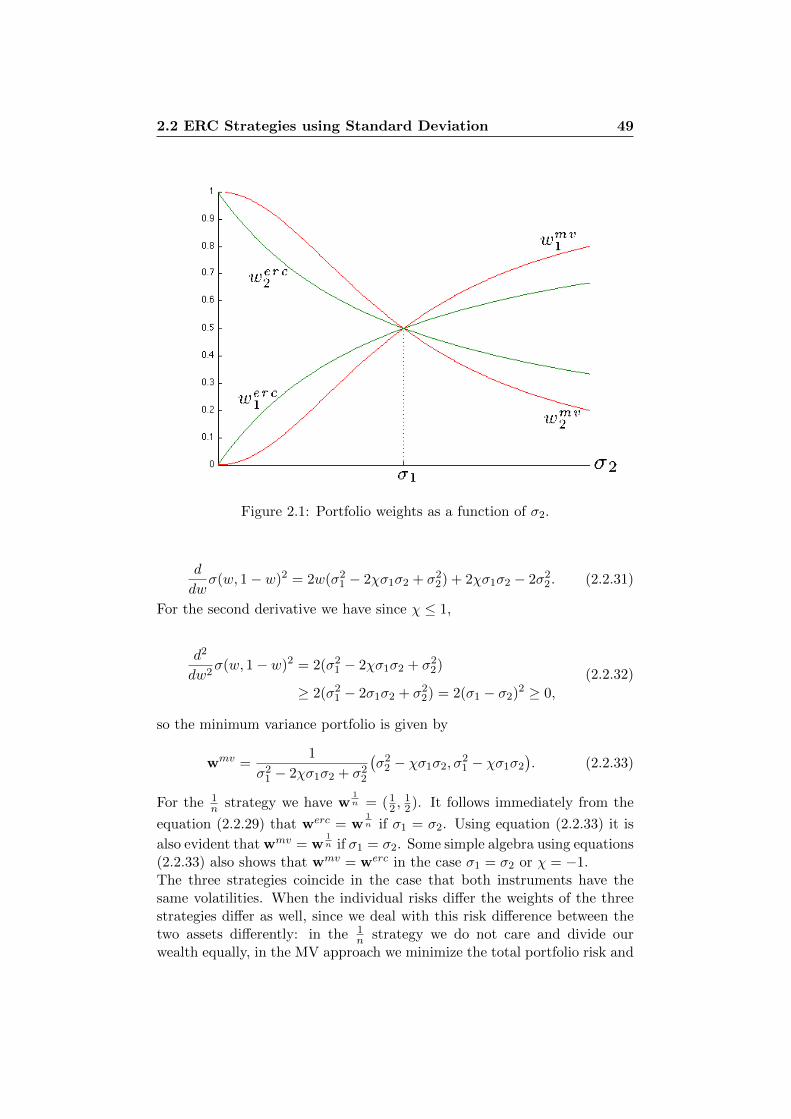
2.2 ERC Strategies using Standard Deviation 49
Figure 2.1: Portfolio weights as a function of σ2.
d
dwσ(w, 1− w)2 = 2w(σ2
1 − 2χσ1σ2 + σ22) + 2χσ1σ2 − 2σ2
2. (2.2.31)
For the second derivative we have since χ ≤ 1,
d2
dw2σ(w, 1− w)2 = 2(σ2
1 − 2χσ1σ2 + σ22)
≥ 2(σ21 − 2σ1σ2 + σ2
2) = 2(σ1 − σ2)2 ≥ 0,
(2.2.32)
so the minimum variance portfolio is given by
wmv =1
σ21 − 2χσ1σ2 + σ2
2
(σ2
2 − χσ1σ2, σ21 − χσ1σ2
). (2.2.33)
For the 1n strategy we have w
1n = (1
2 ,12). It follows immediately from the
equation (2.2.29) that werc = w1n if σ1 = σ2. Using equation (2.2.33) it is
also evident that wmv = w1n if σ1 = σ2. Some simple algebra using equations
(2.2.33) also shows that wmv = werc in the case σ1 = σ2 or χ = −1.The three strategies coincide in the case that both instruments have thesame volatilities. When the individual risks differ the weights of the threestrategies differ as well, since we deal with this risk difference between thetwo assets differently: in the 1
n strategy we do not care and divide ourwealth equally, in the MV approach we minimize the total portfolio risk and
2.2 ERC Strategies using Standard Deviation 50
with the ECR principle we equalize the individual risk components, see alsoFigure 1.
When considering more assets the problem of comparing the results becomesmore involved. Some results are however available. It is for example possibleto show that the ERC portfolio coincides with the MV portfolio when thecorrelation coefficient is minimal. Precisely we have the following ([13] A.1).
Theorem 2.2.2. Assume that the covariance structure of R has constantcorrelation coefficient χ. If the lower bound χ = − 1
n−1 for the correlationcoefficient is achieved then wmv = werc.
Proof. By assumption the covariance matrix has the following form,
Ω = Σ⊗ (χ11′ + (1− χ)In), (2.2.34)
where ⊗ denotes the element by element product, Σij = σiσj and χ is aconstant. For the inverse it holds
Ω−1 = Σ⊗χ11′ −
((n− 1)χ+ 1
)In
(n− 1)χ2 − (n− 2)χ− 1, (2.2.35)
where Σij = 1σiσj
. This follows because,
(χ11′ + (1− χ)In)χ11′ −
((n− 1)χ+ 1
)In
(n− 1)χ2 − (n− 2)χ− 1
=χ2n11′ −
((n− 1)χ+ 1
)χ11′ + (1− χ)χ11′ − (1− χ)
((n− 1)χ+ 1
)In
(n− 1)χ2 − (n− 2)χ− 1
= In.
(2.2.36)
The MV solution is given by
wmvi =(Ω−11)i1′Ω−11
=−((n− 1)χ+ 1
)σ−2i + χ
∑nj=1(σiσj)
−1∑nk=1
(−((n− 1)χ+ 1
)σ−2k + χ
∑nj=1(σkσj)−1
) .(2.2.37)
Substituting χ = − 1n−1 we find
wmvi =
∑nj=1(σiσj)
−1∑nk=1
∑nj=1(σkσj)−1
=σ−1i∑n
k=1 σ−1k
= werci . (2.2.38)
The following which is the main theorem tells us that the ERC portfolio maybe viewed as a compromise between the minimum variance and the equallyweighted portfolio.
2.2 ERC Strategies using Standard Deviation 51
Theorem 2.2.3. For W+l being the set of admissible strategies and a real
constant c consider the following optimization problem,
wopt(c) = arg min√
w′Ωw subject to
∑n
i=1 ln(wi) ≥ c1′w = l
wi ≥ 0 i = 1, . . . , n
. (2.2.39)
There exists a certain cerc ∈ [−∞,−n lnn] such that
wopt(cerc) = werc. (2.2.40)
In particular, this implies that the volatilities of the 1n , MC and ERC strate-
gies are ordered as follows,
σ(wmv) ≤ σ(werc) ≤ σ(w1n ). (2.2.41)
Proof. First observe that if we set c = −∞ there is no additional inequalityconstraint and the above optimization problem is equivalent to the MVproblem. Thus we have wopt(−∞) = wmv. Secondly, applying Jensen’sInequality we find
1
n
n∑i=1
ln(wi) ≤ ln( 1
n
n∑i=1
wi
)= ln(l)− ln(n), (2.2.42)
and so we have the bound∑n
i=1 ln(wi) ≤ n(
ln(l)− ln(n))
for the additional
constraint. This bound is achieved for wi = ln and therefore
wopt(n(
ln(l)− ln(n)))
= w1n . (2.2.43)
Observe also that for c1 ≤ c2 it holds σ(wopt(c1)
)≤ σ
(wopt(c2)
). This is
because the additional constraint becomes more restrictive as the constant cgrows. If we now show that there is a constant cerc ∈ [−∞, n
(ln(l)− ln(n)
)]
corresponding to the ERC strategy, then the inequality (2.2.29) follows di-rectly form the above observations. The existence of such a constant followsdirectly from the work done in the proof of Theorem 2.2.1. For an arbitraryc the solution w∗ of (2.2.22) is an ERC strategy. The ERC solution in W+
l
obtained normalizing w∗ as
werc =l∑n
i=1w∗i
w∗, (2.2.44)
is then the solution of (2.2.39) for cerc = c + n ln(l) − n ln(∑n
i=1w∗i
). By
Jensen’s inequality,

2.3 Other Risk Measures 52
ln( n∑i=1
w∗i
)≥ c
n+ ln(n), (2.2.45)
where we used that∑n
i=1 ln(w∗i ) = c, as seen in the proof of Theorem 2.2.1.The constant cerc satisfies then
cerc ≤ n(
ln(l)− ln(n)). (2.2.46)
This completes the proof.
It is interesting to observe that the ERC portfolio can be obtained from(2.2.39) minimizing the standard deviation as in the MV approach underthe additional condition
n∑i=1
ln(wi) ≥ cerc, (2.2.47)
that can be interpreted as some kind of diversification requirement.
2.3 Other Risk Measures
Obviously the approach of Definition 2.2.1 can be applied to find the op-timal portfolio numerically also when using other risk measures instead ofstandard deviation. It suffices to replace ρi(w) = wi
(Ωw)i
in the aboveequations with the corresponding risk contribution obtained by differentiat-ing the particular risk measure under consideration
RCρi (w) = wi∂ρ
∂wi(w). (2.3.1)
We discuss the formulation of the optimal portfolio problem in the case ofelliptical distributed returns and in the case of Value-at-Risk and ExpectedShortfall.
2.3.1 Elliptical Models
If we assume that R ∼ En(µ,Ω, ψ) there are no particular problems in gen-eralizing the above discussion to other risk measures. Fix a set of acceptablestrategies W and a certain risk measure ρ. We assume in this section that ρis a positive homogeneous, translation invariant and partially differentiablerisk measure. We also assume that ρ depends only on the distribution ofthe profit. Then, by Theorem 1.4.3, the risk contributions for i = 1, . . . , nare given by
RCρi (w) = ρi(w)q − µi, (2.3.2)
2.3 Other Risk Measures 53
where ρi(w) is the risk contribution of the standard deviation and qρ,ψ =q = ρ(Y1) is a constant that depends on the particular ψ of the ellipticalmodel and on the risk measure under consideration. For example: for themultivariate normal model and V aRα we have q = −Φα(α) (see Example1.4.1). The ERC portfolio problem in this case consists in finding a strategywerc such that for all i, j = 1, . . . , n
ρi(werc)− ρj(werc) = −1
q(µi − µj). (2.3.3)
This representation provides some intuition about how the ERC strategy ischosen in the elliptical case. We can observe that here information about theasset returns is used to find the ERC portfolio. The portfolio is chosen sothat for every pair of assets the ratio between the difference of the individualstandard deviation risk contributions and the difference of the returns isconstant. From this it is also evident that the ERC portfolios using ρ andσ as risk measures coincide only if all the assets returns are equal. TheERC problem for σ is therefore a special case of the one for ρ. Also in thiscase no closed-form analytical solutions are available. We can formulate theoptimal portfolio problem in this case as in Definition 2.2.1 using analogousthe functions f1, f2 or fρ0 where ρi is replaced by RCρi . The only thingsthat remains to do is estimating the covariance matrix Ω and the vector ofexpected returns µ. We are going to consider an algorithm to estimate theseparameters in the elliptical model based on historical data in Chapter 3.
2.3.2 VaR and ES for General Models
Assuming that the distribution of R satisfies the necessary assumptions wehave by the work done in Section 1.4 the following risk contributions for aportfolio w,
RCV aRαi (w) = −wiE[Ri
∣∣∣w′R = −V aRα(w)],
RCESαi (w) = −wi1
α
E[Ri1w′R≤qα(w′R)
]+ E
[Ri|w′R = qα(w′R)
](α− P [w′R ≤ qα(w′R)]
),
(2.3.4)
where the last expression in case of continuous profit distribution simplifiesto
RCESαi (w) = −wiE[Ri
∣∣∣w′R ≤ −V aRα(w)]. (2.3.5)
The main difficulty consists therefore in finding estimators for the aboveexpressions. Once such estimators are available we can find the optimalstrategy as explained in Section 2.2. In Chapter 3 we are going to treat the

2.3 Other Risk Measures 54
problem of estimating (2.3.4) and (2.3.5). This quantities can be estimatedwith historical data or using Monte Carlo Methods. There is some new liter-ature proposing methods to estimate these risk contributions by simulation,see for example [20]. We are going to discuss some of the methods based onhistorical data in the next chapter.
Chapter 3
Estimating RiskContributions
3.1 Covariance Matrix Estimation by HistoricalData
In this section we present some covariance matrix estimators for asset re-turns. Suppose we have the return observations r1, . . . , rN , where, fori = 1, . . . , N and j = 1, . . . , n, rij denotes the observation i of the instrumentj. We assume that these returns are independent observations (for differ-ent i) of the same distribution, but no particular form of the distributionsuch as normal is assumed. We also assume that the distribution is suchthat second moments exist. The independence assumption of asset returnsthrough time is actually not verified but it is an acceptable approximation.The question of constructing covariance matrix estimators using the datais a very important issue in finance, especially in the context of this thesiswhere in order to estimate the risk contributions of the assets in the port-folio we often need to estimate the covariances between the asset returns.The standard estimators for the expected returns and the covariances arethe sample estimators, defined by
r =1
N
N∑i=1
ri, Ω =1
N
N∑i=1
(ri − r)(rj − r)′. (3.1.1)
The estimator r is an unbiased estimator for the vector of expected returns,but Ω is not unbiased for Ω. An unbiased version can be obtained by n
n−1 Ω
as it can immediately be verified computing E[Ω]. The sample covariancematrix estimator Ω has the appealing property of being the maximum like-lihood estimator under normally distributed asset returns, i.e. the samplecovariances are the most likely parameters value given the data. Covariancematrices are always positive semi-definte. The sample covariance matrix
3.1 Covariance Matrix Estimation by Historical Data 56
estimator produces always a positive semi-definite matrix as shown in thefollowing example.
Example 3.1.1. Let r1, . . . , rN ∈ Rn be N data vectors. Define a randomvector X with Xj ∈ r1j , . . . , rNj for j = 1, . . . , n and
P [Xi = ri] =1
N, (3.1.2)
for i = 1, . . . , N . Note that, if some of the data vectors are equal to eachothers, the above probabilities need to be modified. The random vector Xhas the following properties
E[X] =1
N
N∑i=1
ri = r,
Cov(X) = E[(X− E[X])(X− E[X])′
]=
1
N
N∑i=1
(ri − r)(ri − r)′ = Ω.
(3.1.3)
The true covariance matrix of this random vector is equal to the samplecovariance matrix of the data set r1, . . . , rN . Since a true covariance matrixis known to be positive semi-definite, then it follows that also the samplecovariance matrix estimator is also positive semi-definite.
Despite these nice properties sample covariance matrices present some seri-ous deficiencies. The sample estimator let the data speak and only the data.But what about if we are in a situation where there are not enough data togive full weight to the them? In the situation where we have more assetsthan data the sample estimation is obviously problematic since there aremore parameters to estimate than historical returns. The sample covariancematrix can be written in matrix notation as
Ω =1
NR′(I − 1
N11′)R, (3.1.4)
where R = (rij)1≤i≤N,1≤j≤n is the matrix of observations, I ∈ RN×N is theidentity matrix and 1 ∈ RN is the vector of ones. From the above equationit follows that whenever n exceeds N − 1, the sample covariance matrix isrank-deficient. This is because the rank of Ω is at most equal to the rank ofthe matrix I − 1
N 11′, which is N − 1. Whenever we have n ≥ N the sampleestimator always lead to a singular matrix even if the true covariance matrixis assumed to be non-singular. Because of this, we need to modify the sampleestimator. Small samples situations are often considered in the context ofportfolio construction where we want for example to choose portfolio weightsamong several hundreds of financial instruments using the daily observations
3.1 Covariance Matrix Estimation by Historical Data 57
of the last three months. Obtaining a singular estimated covariance matrix isvery problematic in the context of this thesis. For example, it is problematicin the context of risk contributions for the standard deviation risk measurewhere we assume that σ2(w) = w′Ωw > 0, i.e. that the covariance matrixis positive definite. The method we want to present is usually referred to inthe literature as shrinkage and it consists in combining the asymptoticallyunbiased sample covariance matrix estimator Ω with another biased highlystructured estimator, denoted by F . We want for our final estimator tobe a compromise between the two estimators and we consider therefore thecredibility weighted average
Ω(α) = αF + (1− α)Ω, (3.1.5)
for α ∈ (0, 1). The estimator F is referred to in the literature as the prior es-timator or shrinking target and α as shrinkage constant or credibility weight,since the sample estimator is ”shrunk” towards the structured estimator. Itis important to explain more precisely what we mean when say that wewant F to be an estimator with lot of structure: we want F to be a matrixthat involve only a small number of free parameters and that at the sametime captures important information on the true covariance matrix. Thisapproach is very similar to the one used in Bayesian statistics where thesame convex linear combinations are considered to give at the same timeweight to the data and to other beliefs about the problem under consid-eration. Choosing a proper shrinking target is an issue that depends onthe estimation problem under consideration, in the context of estimatingstock returns covariances Ledoit and Wolf [11] have for example proposed aprior based on Sharpe’s single-index model for stocks returns. However, themethodology proposed by the authors does not rely strongly on the chosentarget and can be applied more generally. Ledoit and Wolf [12] present ina sequent paper an estimator that is quite easy to implement and which isbased on a prior covariance matrix with constant correlation coefficient. Weare going to formulate and use this estimator which is known to perform wellin the context of portfolio construction. Another advantage of this shrinkageestimator is that it is always positive definite, since it is a convex combina-tion of an estimator that is positive definite (the shrinkage target F) andan estimator that is positive semi-definite (the sample estimator). We starttherefore with the constant correlation model as prior which states that allthe pairwise asset correlations are identical. This clearly imposes a particu-lar covariance matrix structure that can be estimated by using the averageof all the sample correlations as common constant correlation together withthe sample variances. Formally, if we denote by χij the true correlation co-efficient between assets i and j, then we define the true constant correlationmatrix by
3.1 Covariance Matrix Estimation by Historical Data 58
φii = Ωii, φij = χ√
ΩiiΩjj , (3.1.6)
where Ω denotes the true covariance matrix and
χ =2
(n− 1)n
n−1∑i=1
n∑j=i+1
χij . (3.1.7)
Our shrinking target is then defined as the sample constant correlation ma-trix
Fii = Ωii, Fij = χ
√ΩiiΩjj , (3.1.8)
where
χ =2
(n− 1)n
n−1∑i=1
n∑j=i+1
χij , χij =Ωij√ΩiiΩjj
. (3.1.9)
The obvious question is now how the parameter α should be selected. Weuse the following optimality criterion.
Definition 3.1.1. The optimal shrinkage intensity α∗ is defined as
α∗ = arg minα∈[0,1]E[∣∣Ω− Ω(α)
∣∣2F
], (3.1.10)
where Ω(α) defines, as a function of the observations, a random variable and| · |F denotes the Frobenius norm defined by
|A|2F =n∑
i,j=1
A2ij , (3.1.11)
for any matrix A ∈ Rn×n.
The key result, which provides an asymptotic description of the optimalshrinkage intensity, and is independent of the particular structured estima-tor under consideration is [11] Theorem 1. This result states (under someassumptions about finite variances in order to be able to apply the centrallimit theorem) that, for the following quantities,
π =n∑
i,j=1
AsyV ar[√N Ωij ],
ρ =n∑
i,j=1
AsyCov(√NFij ,
√N Ωij ],
γ =
n∑i,j=1
(φij − Ωij
)2,
(3.1.12)
3.2 Estimating VaR and ES Risk Contributions by HistoricalData 59
we have,
α∗ =1
N
π − ργ
+O( 1
N2
), (3.1.13)
as N →∞. This result allows to estimate the optimal shrinkage intensity byfinding consistent estimators π, ρ and γ for the above quantities. Consistentestimators for π and γ can be found independently of the chosen prior andare given by
π =n∑
i,j=1
πij , πij =1
N
T∑k=1
[(rki −
1
N
N∑l=1
rli
)(rkj −
1
N
N∑l=1
rlj
)− Ωij
]2
,
γ =N∑
i,j=1
(Fij − Ωij
)2,
(3.1.14)
as proven in [11] Lemma 1 and Lemma 3. Expressions to estimate ρ needhowever to be readjusted for different priors. A consistent estimator in thiscase is computed in [12] Appendix B and given by,
ρ =n∑i=1
πii +n∑i=1
n∑j=1,j 6=i
χ
2
(√Ωjj
Ωii
ϑii,ij +
√Ωii
Ωjj
ϑjj,ij
), (3.1.15)
where ϑii,ij and ϑjj,ij are the consistent estimator of the asymptotic covari-ances AsyCov(
√N Ωii,
√N Ωij) and AsyCov(
√N Ωjj ,
√T Ωij) given in [12]
Appendix B. Now we have all the elements to apply this shrinkage estima-tor. We are going to use this estimator when estimating risk contributionsthat require covariance matrix estimation.
3.2 Estimating VaR and ES Risk Contributions byHistorical Data
As in the previous section we use the notation rij , for i = 1, . . . , N andj = 1, . . . , n, to indicate independent (w.r.t. i) return observations of thesame distribution. We also assume that the distribution of the returns is niceenough so that the representations (2.3.4) and (2.3.5) for the risk contribu-tions are available. We want to use this conditional expectations to estimatethe risk contributions using historical return data. For certain portfoliow ∈ Rn, we define the vector of observed portfolio returns x = (x1, . . . , xN )by
xi = w′ri, (3.2.1)

3.2 Estimating VaR and ES Risk Contributions by HistoricalData 60
for i = 1, . . . , N . If the number of observations N is large, then by the lawof large numbers the portfolio return distribution can be approximated bythe empirical distribution based on the historical portfolio return data:
P (X ≤ x) ≈ #i = 1, . . . , N |xi ≤ xN
. (3.2.2)
The VaR and ES risk measures can then be approximated with
V aRα(w) ≈ −xsortdαNe,
ESα(w) ≈ − 1
bαNc
bαNc∑i=1
xsorti ,(3.2.3)
where xsort1 ≤ · · · ≤ xsortN denote the sorted portfolio returns. From (2.3.5)it is clear how to use historical data to approximate ES risk contribution.
RCESαi (w) = −E[Ri|X ≤ −V aRα(X)] ≈ − 1
bαNc
bαNc∑k=1
rsortki , (3.2.4)
where rsortki are the corresponding asset returns to the sorted portfolio re-turns. The estimation of VaR is because of the equality condition muchmore problematic. A possible way of doing it, it is using a gaussian kernelestimation for some fixed bandwidth b > 0:
RCV aRαi (w) = −E[Ri|X = −V aRα(X)] ≈ −
∑Nk=1 rkiϕ
(−V aRα(X)−xk
b
)∑N
k=1 ϕ(−V aRα(X)−xk
b
) ,
(3.2.5)where V aRα(X) can be approximated as in (3.2.3). The main problem ofthis method is that there is no general rule for fixing b and the choice ofthe bandwidth is quite crucial in order to get accurate approximation. Wewill fix the parameter b on a case-by-case basis by numerical experiments.We can measure how accurate the above approximation is by comparing∑n
i=1RCV aRαi (w) with the value of V aRα(w) obtained with (3.2.3).
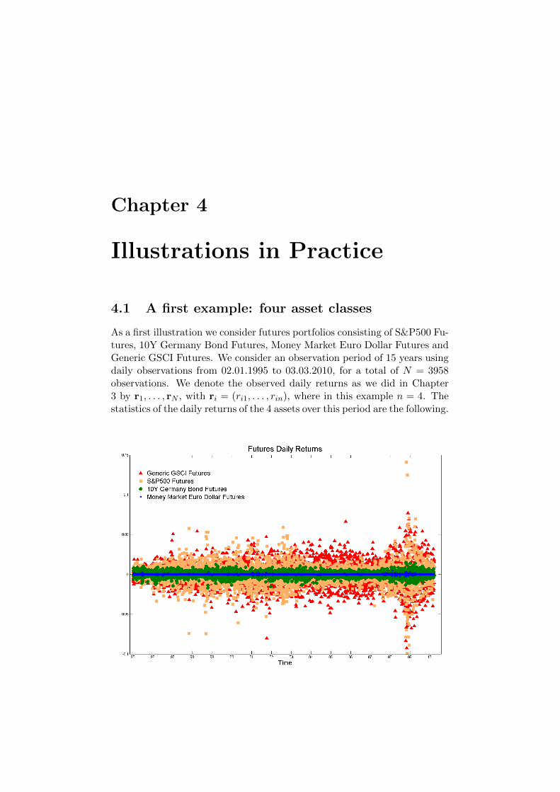
Chapter 4
Illustrations in Practice
4.1 A first example: four asset classes
As a first illustration we consider futures portfolios consisting of S&P500 Fu-tures, 10Y Germany Bond Futures, Money Market Euro Dollar Futures andGeneric GSCI Futures. We consider an observation period of 15 years usingdaily observations from 02.01.1995 to 03.03.2010, for a total of N = 3958observations. We denote the observed daily returns as we did in Chapter3 by r1, . . . , rN , with ri = (ri1, . . . , rin), where in this example n = 4. Thestatistics of the daily returns of the 4 assets over this period are the following.
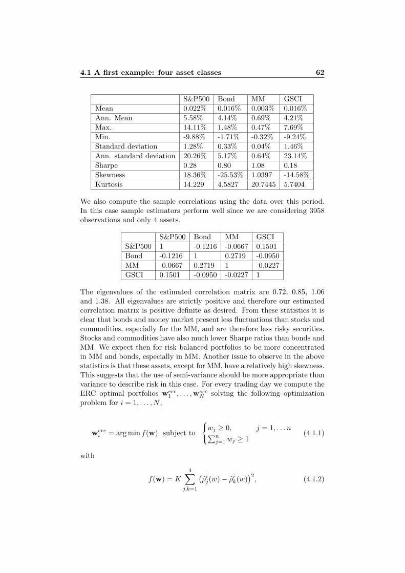
4.1 A first example: four asset classes 62
S&P500 Bond MM GSCI
Mean 0.022% 0.016% 0.003% 0.016%
Ann. Mean 5.58% 4.14% 0.69% 4.21%
Max. 14.11% 1.48% 0.47% 7.69%
Min. -9.88% -1.71% -0.32% -9.24%
Standard deviation 1.28% 0.33% 0.04% 1.46%
Ann. standard deviation 20.26% 5.17% 0.64% 23.14%
Sharpe 0.28 0.80 1.08 0.18
Skewness 18.36% -25.53% 1.0397 -14.58%
Kurtosis 14.229 4.5827 20.7445 5.7404
We also compute the sample correlations using the data over this period.In this case sample estimators perform well since we are considering 3958observations and only 4 assets.
S&P500 Bond MM GSCI
S&P500 1 -0.1216 -0.0667 0.1501
Bond -0.1216 1 0.2719 -0.0950
MM -0.0667 0.2719 1 -0.0227
GSCI 0.1501 -0.0950 -0.0227 1
The eigenvalues of the estimated correlation matrix are 0.72, 0.85, 1.06and 1.38. All eigenvalues are strictly positive and therefore our estimatedcorrelation matrix is positive definite as desired. From these statistics it isclear that bonds and money market present less fluctuations than stocks andcommodities, especially for the MM, and are therefore less risky securities.Stocks and commodities have also much lower Sharpe ratios than bonds andMM. We expect then for risk balanced portfolios to be more concentratedin MM and bonds, especially in MM. Another issue to observe in the abovestatistics is that these assets, except for MM, have a relatively high skewness.This suggests that the use of semi-variance should be more appropriate thanvariance to describe risk in this case. For every trading day we compute theERC optimal portfolios werc
1 , . . . ,wercN solving the following optimization
problem for i = 1, . . . , N ,
werci = arg min f(w) subject to
wj ≥ 0, j = 1, . . . n∑n
j=1wj ≥ 1(4.1.1)
with
f(w) = K4∑
j,k=1
(ρij(w)− ρik(w)
)2, (4.1.2)

4.1 A first example: four asset classes 63
where ρij denotes the estimated risk contribution of the instrument j at dayi, and K ∈ R is a constant. We optimize with long constraint but allowingfor arbitrary leverage, the desired leverage can then be obtained normalizingthe solution. The factor K in (4.1.2) allows to fasten the optimization: dailyrisk contributions in this example are pretty small numbers that make theoptimization problematic, rescaling with some K big enough helps solvingthe optimization more efficiently. In this example we used K = 104 andobtained quite good approximations of the minimum. For the daily portfolioweights of our strategy we can compute using the returns data the dailyportfolio returns x = (x1, . . . , xN ) setting xi = r′iw
erci . Using these N
values that depend only on the chosen strategy and on the market data wedefine the following statistical quantities that we are going to use to measureperformance and to compare strategies. We define the mean daily portfolioreturn by
µ(x) =1
N
N∑i=1
xi. (4.1.3)
The annualized mean portfolio return is then given by
µ(x)ann =(1 + µ(x)
)250 − 1, (4.1.4)
where we take the power 250 since there are approximately so many tradingdays in a year. Note that mean returns are going to be used in order toquantify relationships between portfolio risk and return. To quantify thetotal gain of the strategy we compute for k = 1, . . . , N the compoundedreturn,
µck(x) =k∏i=1
(1 + xi)− 1, (4.1.5)
and we denote by µc(x) = µcN (x) the compounded return over the wholeperiod. As measures of risk of the strategy we compute the sample volatility,value-at-risk and expected shortfall of the daily returns over the period.
σ(x) =
(1
N
N∑i=1
(xi − µ(x))2
) 12
,
V aRα(x) = −xsortdNαe,
ESα(x) = − 1
bNαc
bNαc∑i=1
xsorti .
(4.1.6)
These represent daily risks and can be annualized by multiplying them withthe factor
√250. Note that this is the right scaling factor in the case of nor-
4.1 A first example: four asset classes 64
mally distributed data (see [17] Example 2.23), with no distribution assump-tion, this is just a definition of how we annualize risks. For the annualizedrisks we use the notation σ(x)ann, V aRα(x)ann and ESα(x)ann. Also veryrelevant quantities for many asset management firms are the drawdowns ofthe strategy and in particular the maximum drawdown:
DDi(x) = max1≤k≤i
µck(x)− µci (x),
MDD(x) = max1≤i≤N
DDi(x).(4.1.7)
We will then consider the following performance ratios: Sσ(x) = µ(x)annσ(x)ann
,
SV aR(x) = µ(x)annV aRα(x)ann
, SES(x) = µ(x)annESα(x)ann
, SDD(x) = µ(x)1N
∑Ni=1DDi(x)
and
SMDD(x) = µ(x)MDD(x) . Another very important quantity in practice is the
portion we need to trade in order to apply a certain investment strategy. Toquantify this we define the strategy turnover as
TOi(w1, . . . ,wN ) =i−1∑k=1
|wk+1 −wk|1 (4.1.8)
where |w|1 = |w1| + · · · + |wn| denotes the 1-norm, and we denote theterminal turnover by TO(w1, . . . ,wN ) = TON (w1, . . . ,wN ). The meandaily turnover can be annualized by multiplying it with 250. We now exposeour results for the ERC strategy using different risk measures and differentdistribution assumptions. We have implemented everything using Matlab7.8.0. Our implementation consists essentially in using the Matlab functionfmincon (see Appendix C) properly to solve the optimization.
4.1.1 Standard Deviation
We consider the ERC strategy using the standard deviation as risk measure.For every trading day we estimate the covariance matrix of the returns dis-tribution using the previous 100 daily returns and the shrinkage procedure ofSection 3.2 selecting as prior a covariance matrix with constant correlationcoefficient. For this example the difference between shrinkage estimationand sample covariances is however not so pronounced since we are consid-ering 100 data per instrument and only 4 instruments. The eigenvaluesof the estimated covariance matrix for every trading day are positive andrepresented in the following figure.
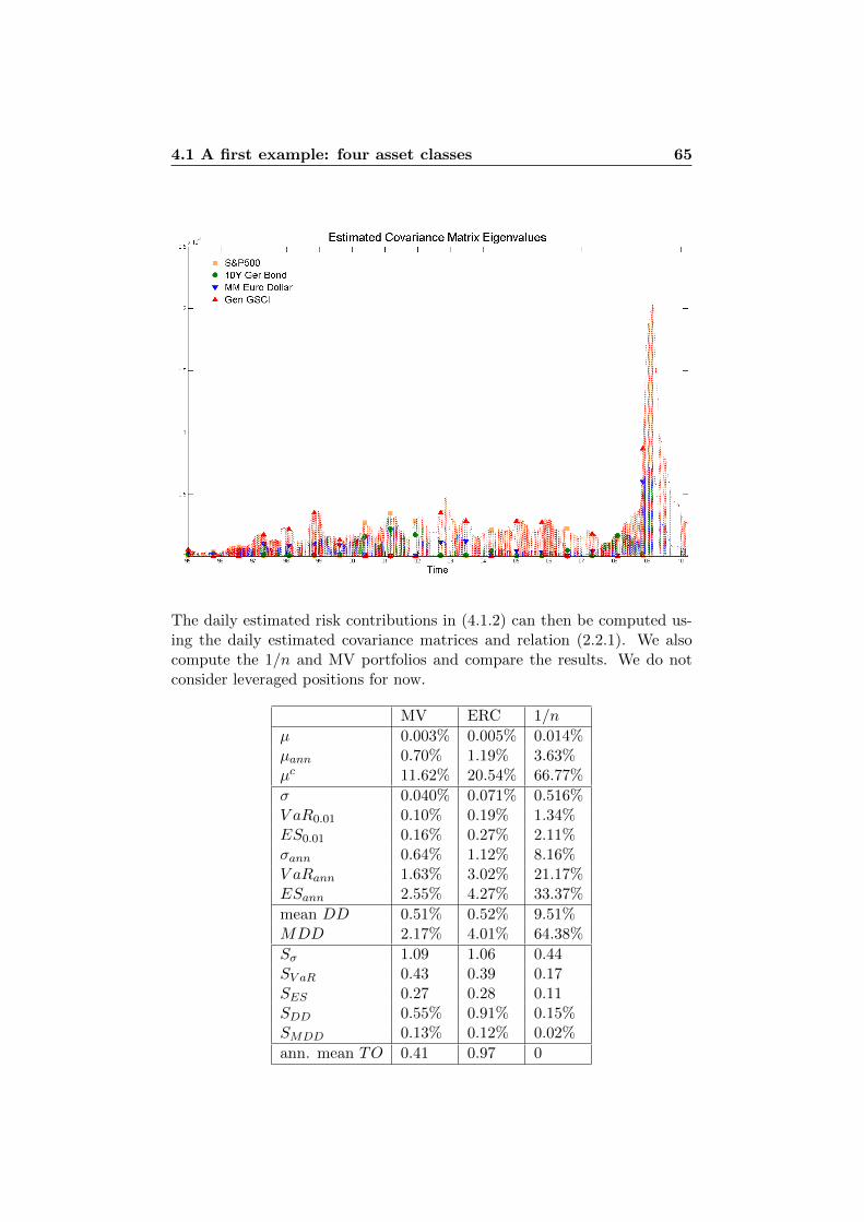
4.1 A first example: four asset classes 65
The daily estimated risk contributions in (4.1.2) can then be computed us-ing the daily estimated covariance matrices and relation (2.2.1). We alsocompute the 1/n and MV portfolios and compare the results. We do notconsider leveraged positions for now.
MV ERC 1/n
µ 0.003% 0.005% 0.014%µann 0.70% 1.19% 3.63%µc 11.62% 20.54% 66.77%
σ 0.040% 0.071% 0.516%V aR0.01 0.10% 0.19% 1.34%ES0.01 0.16% 0.27% 2.11%σann 0.64% 1.12% 8.16%V aRann 1.63% 3.02% 21.17%ESann 2.55% 4.27% 33.37%
mean DD 0.51% 0.52% 9.51%MDD 2.17% 4.01% 64.38%
Sσ 1.09 1.06 0.44SV aR 0.43 0.39 0.17SES 0.27 0.28 0.11SDD 0.55% 0.91% 0.15%SMDD 0.13% 0.12% 0.02%
ann. mean TO 0.41 0.97 0
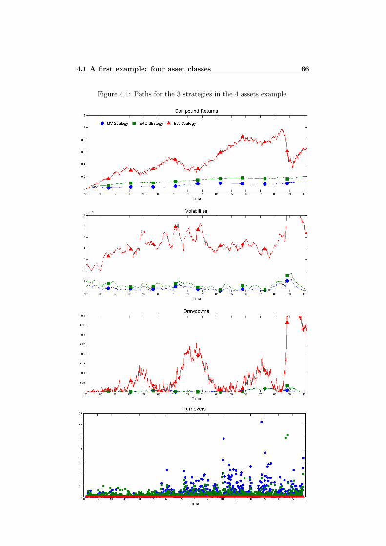
4.1 A first example: four asset classes 66
Figure 4.1: Paths for the 3 strategies in the 4 assets example.
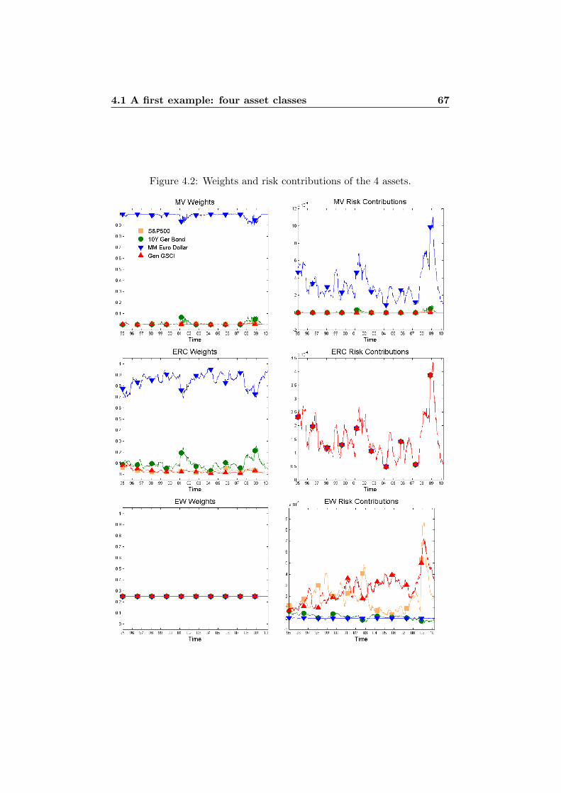
4.1 A first example: four asset classes 67
Figure 4.2: Weights and risk contributions of the 4 assets.
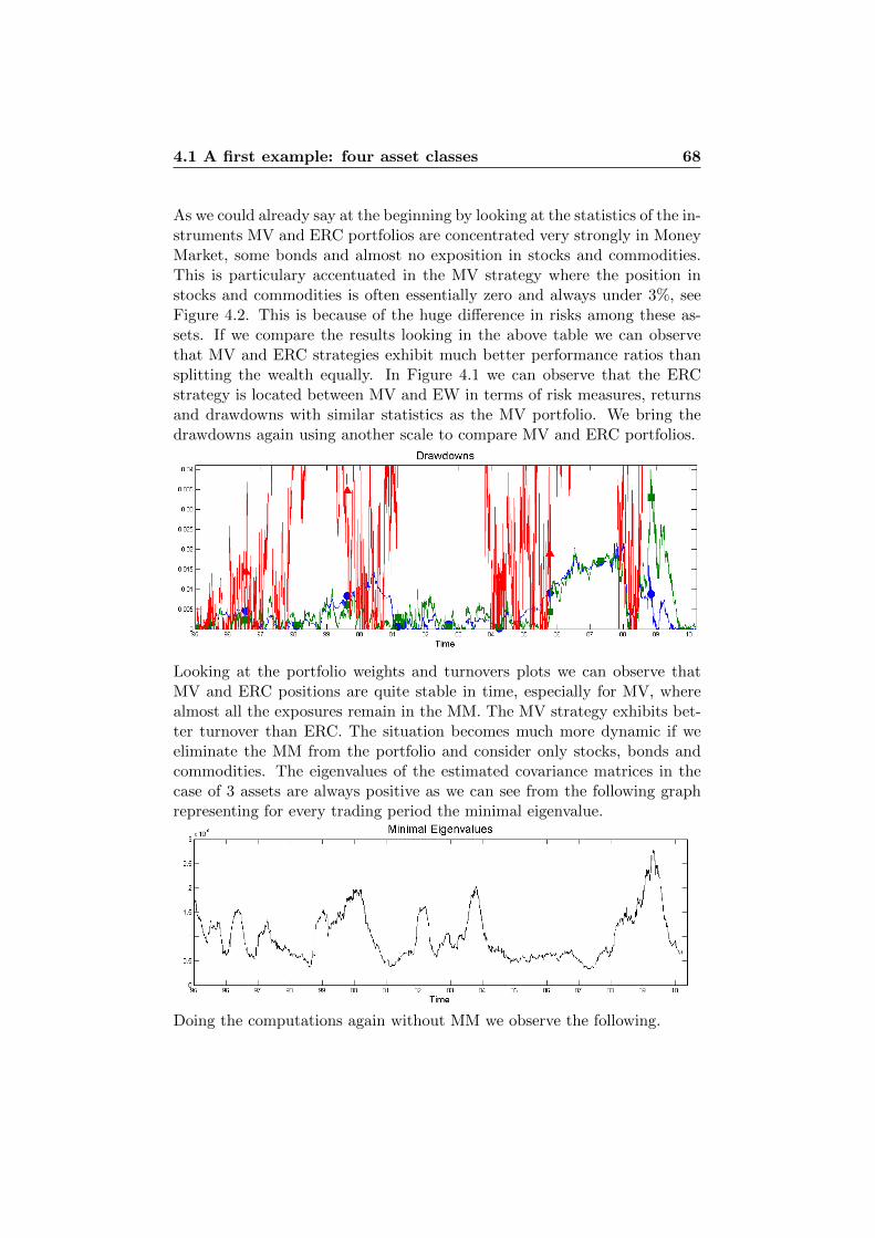
4.1 A first example: four asset classes 68
As we could already say at the beginning by looking at the statistics of the in-struments MV and ERC portfolios are concentrated very strongly in MoneyMarket, some bonds and almost no exposition in stocks and commodities.This is particulary accentuated in the MV strategy where the position instocks and commodities is often essentially zero and always under 3%, seeFigure 4.2. This is because of the huge difference in risks among these as-sets. If we compare the results looking in the above table we can observethat MV and ERC strategies exhibit much better performance ratios thansplitting the wealth equally. In Figure 4.1 we can observe that the ERCstrategy is located between MV and EW in terms of risk measures, returnsand drawdowns with similar statistics as the MV portfolio. We bring thedrawdowns again using another scale to compare MV and ERC portfolios.
Looking at the portfolio weights and turnovers plots we can observe thatMV and ERC positions are quite stable in time, especially for MV, wherealmost all the exposures remain in the MM. The MV strategy exhibits bet-ter turnover than ERC. The situation becomes much more dynamic if weeliminate the MM from the portfolio and consider only stocks, bonds andcommodities. The eigenvalues of the estimated covariance matrices in thecase of 3 assets are always positive as we can see from the following graphrepresenting for every trading period the minimal eigenvalue.
Doing the computations again without MM we observe the following.
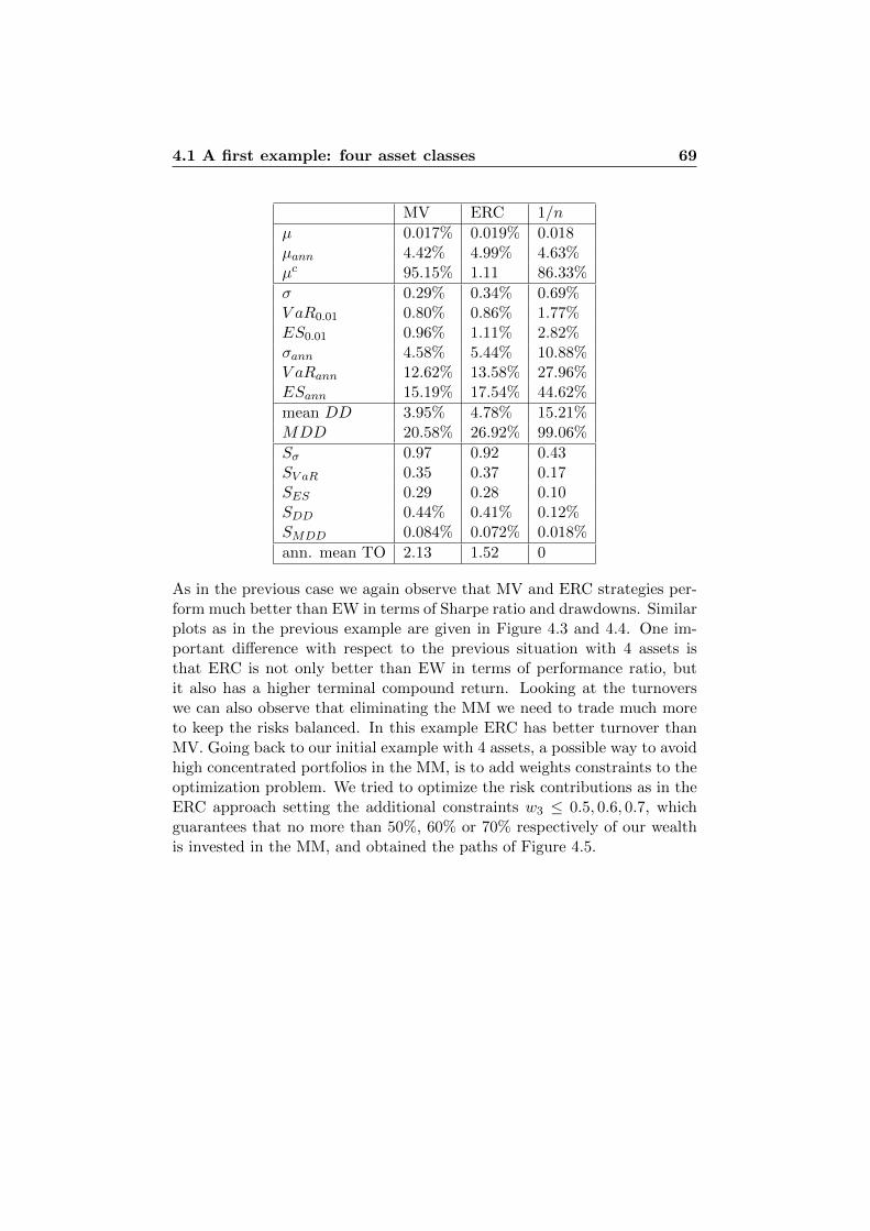
4.1 A first example: four asset classes 69
MV ERC 1/n
µ 0.017% 0.019% 0.018µann 4.42% 4.99% 4.63%µc 95.15% 1.11 86.33%
σ 0.29% 0.34% 0.69%V aR0.01 0.80% 0.86% 1.77%ES0.01 0.96% 1.11% 2.82%σann 4.58% 5.44% 10.88%V aRann 12.62% 13.58% 27.96%ESann 15.19% 17.54% 44.62%
mean DD 3.95% 4.78% 15.21%MDD 20.58% 26.92% 99.06%
Sσ 0.97 0.92 0.43SV aR 0.35 0.37 0.17SES 0.29 0.28 0.10SDD 0.44% 0.41% 0.12%SMDD 0.084% 0.072% 0.018%
ann. mean TO 2.13 1.52 0
As in the previous case we again observe that MV and ERC strategies per-form much better than EW in terms of Sharpe ratio and drawdowns. Similarplots as in the previous example are given in Figure 4.3 and 4.4. One im-portant difference with respect to the previous situation with 4 assets isthat ERC is not only better than EW in terms of performance ratio, butit also has a higher terminal compound return. Looking at the turnoverswe can also observe that eliminating the MM we need to trade much moreto keep the risks balanced. In this example ERC has better turnover thanMV. Going back to our initial example with 4 assets, a possible way to avoidhigh concentrated portfolios in the MM, is to add weights constraints to theoptimization problem. We tried to optimize the risk contributions as in theERC approach setting the additional constraints w3 ≤ 0.5, 0.6, 0.7, whichguarantees that no more than 50%, 60% or 70% respectively of our wealthis invested in the MM, and obtained the paths of Figure 4.5.
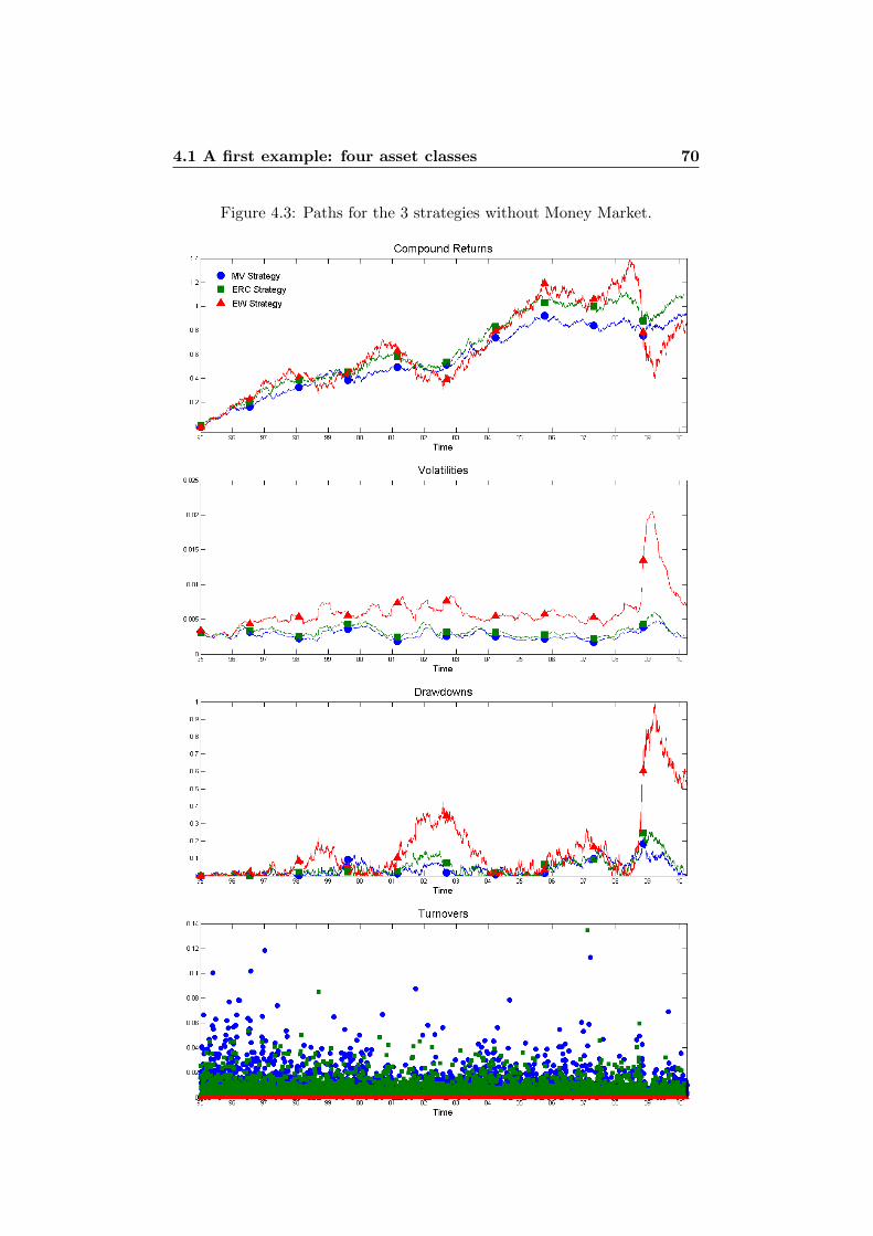
4.1 A first example: four asset classes 70
Figure 4.3: Paths for the 3 strategies without Money Market.
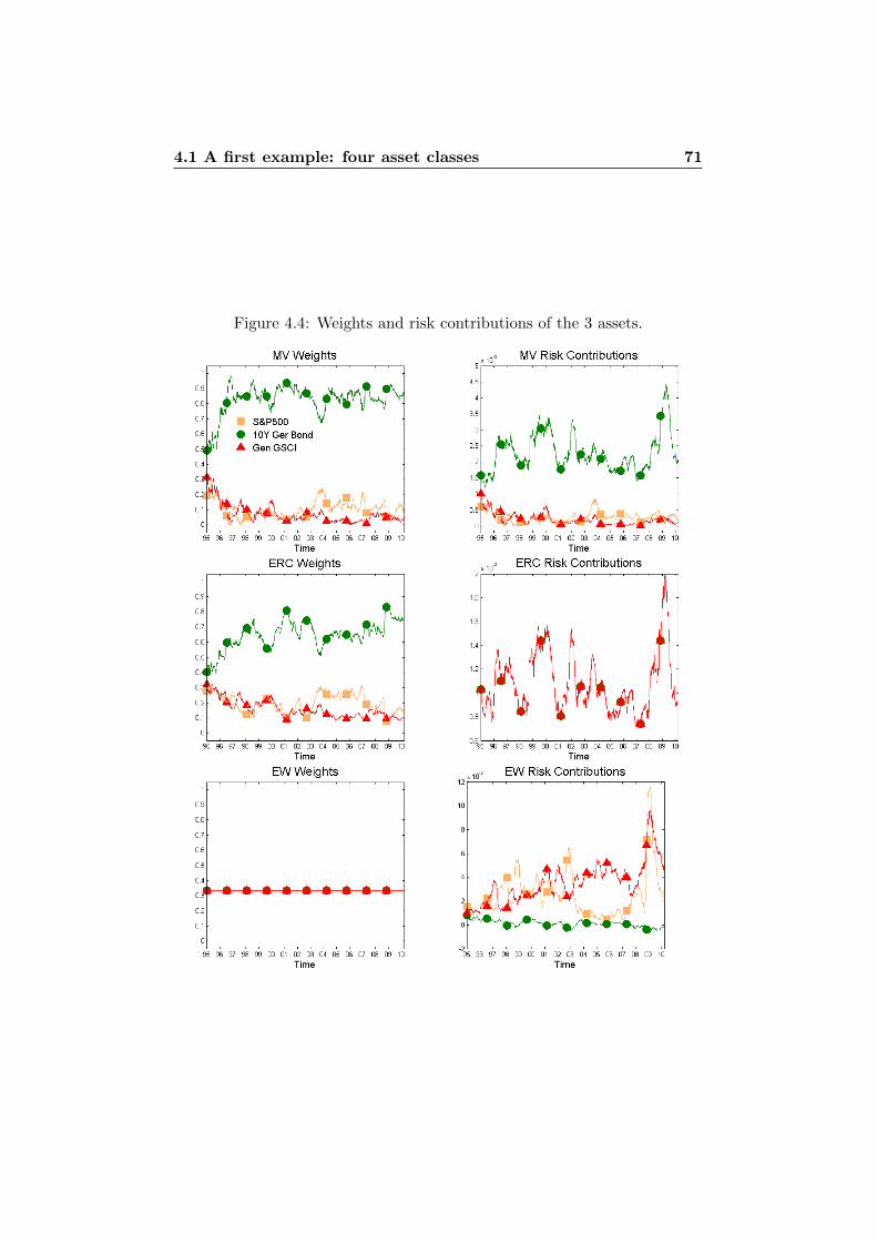
4.1 A first example: four asset classes 71
Figure 4.4: Weights and risk contributions of the 3 assets.

4.1 A first example: four asset classes 72
Figure 4.5: Using weights constraints.
unconstraint 0.7 0.6 0.5
µ 0.005% 0.008% 0.009% 0.011%µann 1.19% 1.94% 2.36% 2.78%µc 20.54% 35.18% 44.13% 53.52%
σ 0.071% 0.11% 0.14% 0.17%V aR0.01 0.19% 0.28% 0.36% 0.44%ES0.01 0.27% 0.35% 0.45% 0.55%σann 1.12% 1.73% 2.23% 2.73%V aRann 3.02% 4.36% 5.67% 6.96%ESann 4.27% 5.47% 7.05% 8.68%
mean DD 0.52% 0.85% 1.17% 1.57%MDD 4.01% 5.18% 7.25% 9.67%
Sσ 1.06 1.12 1.06 1.02SV aR 0.39 0.44 0.42 0.4SES 0.28 0.35 0.34 0.32SDD 0.91% 0.90% 0.80% 0.70%SMDD 0.12% 0.15% 0.13% 0.11%
ann. mean TO 97% 49.34% 63.77% 79.19%
Here we can observe something very interesting: imposing constraint tothe money invested in the MM, we get portfolios with higher returns andhigher risks and drawdowns, however without affecting the performance ra-tios strongly. If we consider for example a 50% constraint in the MM weobtain a twice as big mean daily return with respect to the unconstraintERC solution. Additionally, we observe that the Sharpe ratio remains very
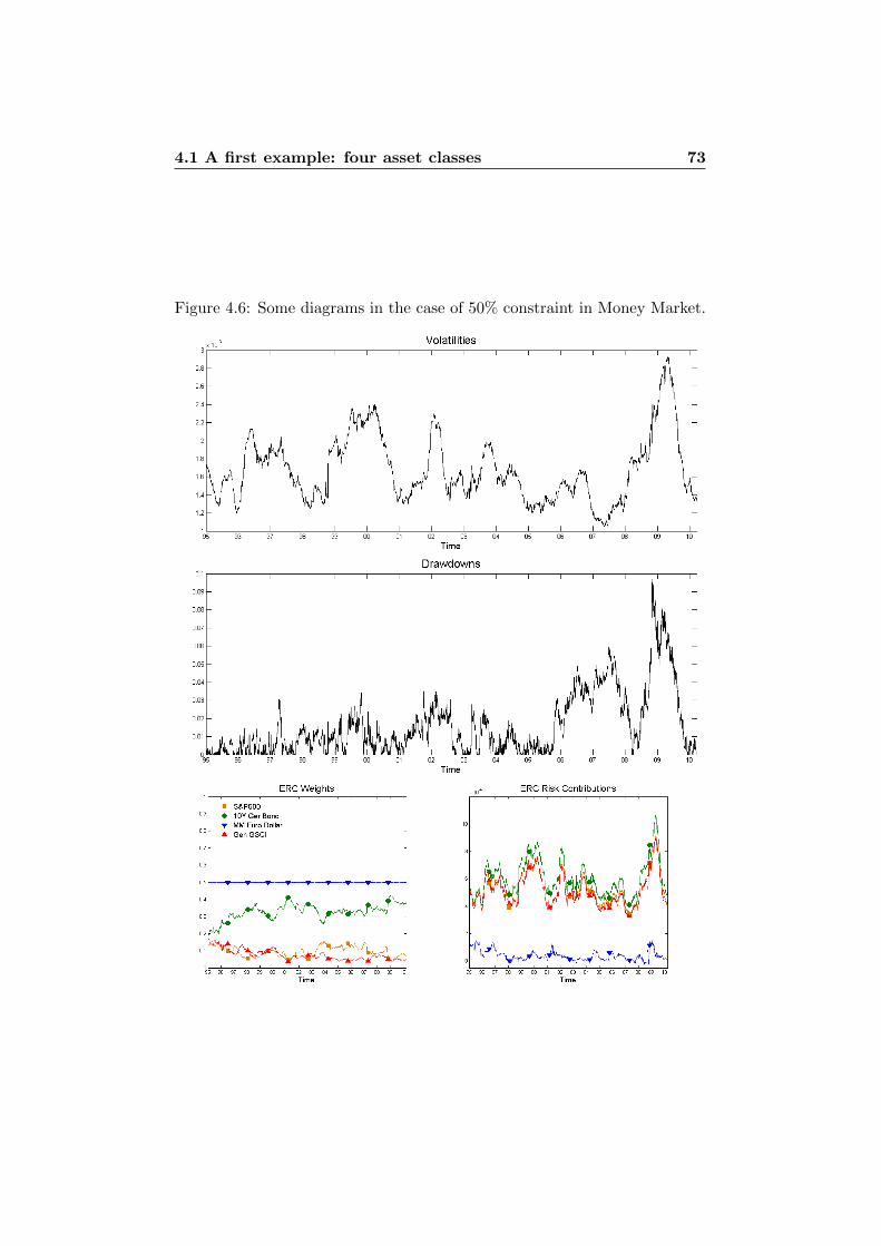
4.1 A first example: four asset classes 73
Figure 4.6: Some diagrams in the case of 50% constraint in Money Market.
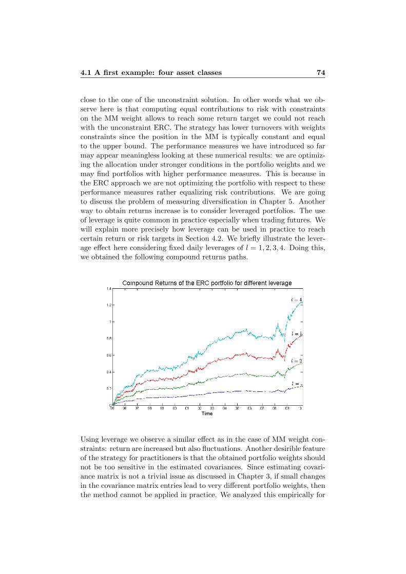
4.1 A first example: four asset classes 74
close to the one of the unconstraint solution. In other words what we ob-serve here is that computing equal contributions to risk with constraintson the MM weight allows to reach some return target we could not reachwith the unconstraint ERC. The strategy has lower turnovers with weightsconstraints since the position in the MM is typically constant and equalto the upper bound. The performance measures we have introduced so farmay appear meaningless looking at these numerical results: we are optimiz-ing the allocation under stronger conditions in the portfolio weights and wemay find portfolios with higher performance measures. This is because inthe ERC approach we are not optimizing the portfolio with respect to theseperformance measures rather equalizing risk contributions. We are goingto discuss the problem of measuring diversification in Chapter 5. Anotherway to obtain returns increase is to consider leveraged portfolios. The useof leverage is quite common in practice especially when trading futures. Wewill explain more precisely how leverage can be used in practice to reachcertain return or risk targets in Section 4.2. We briefly illustrate the lever-age effect here considering fixed daily leverages of l = 1, 2, 3, 4. Doing this,we obtained the following compound returns paths.
Using leverage we observe a similar effect as in the case of MM weight con-straints: return are increased but also fluctuations. Another desirible featureof the strategy for practitioners is that the obtained portfolio weights shouldnot be too sensitive in the estimated covariances. Since estimating covari-ance matrix is not a trivial issue as discussed in Chapter 3, if small changesin the covariance matrix entries lead to very different portfolio weights, thenthe method cannot be applied in practice. We analyzed this empirically for
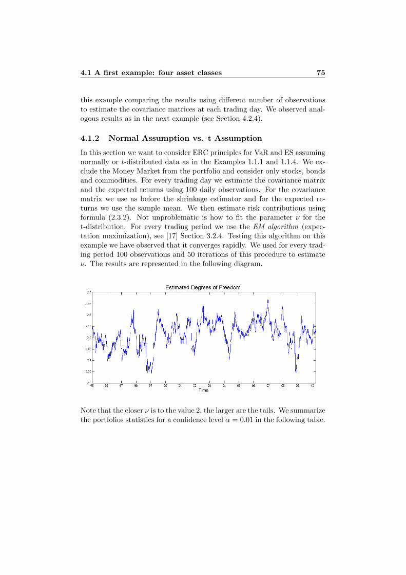
4.1 A first example: four asset classes 75
this example comparing the results using different number of observationsto estimate the covariance matrices at each trading day. We observed anal-ogous results as in the next example (see Section 4.2.4).
4.1.2 Normal Assumption vs. t Assumption
In this section we want to consider ERC principles for VaR and ES assumingnormally or t-distributed data as in the Examples 1.1.1 and 1.1.4. We ex-clude the Money Market from the portfolio and consider only stocks, bondsand commodities. For every trading day we estimate the covariance matrixand the expected returns using 100 daily observations. For the covariancematrix we use as before the shrinkage estimator and for the expected re-turns we use the sample mean. We then estimate risk contributions usingformula (2.3.2). Not unproblematic is how to fit the parameter ν for thet-distribution. For every trading period we use the EM algorithm (expec-tation maximization), see [17] Section 3.2.4. Testing this algorithm on thisexample we have observed that it converges rapidly. We used for every trad-ing period 100 observations and 50 iterations of this procedure to estimateν. The results are represented in the following diagram.
Note that the closer ν is to the value 2, the larger are the tails. We summarizethe portfolios statistics for a confidence level α = 0.01 in the following table.
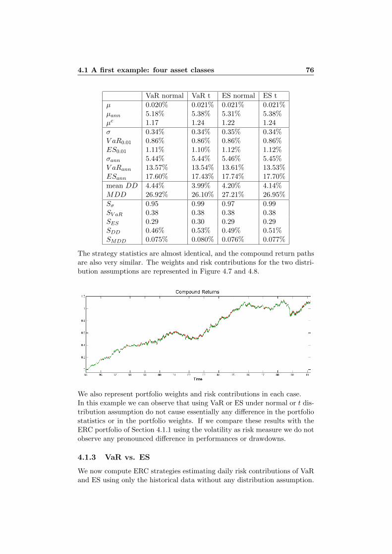
4.1 A first example: four asset classes 76
VaR normal VaR t ES normal ES t
µ 0.020% 0.021% 0.021% 0.021%µann 5.18% 5.38% 5.31% 5.38%µc 1.17 1.24 1.22 1.24
σ 0.34% 0.34% 0.35% 0.34%V aR0.01 0.86% 0.86% 0.86% 0.86%ES0.01 1.11% 1.10% 1.12% 1.12%σann 5.44% 5.44% 5.46% 5.45%V aRann 13.57% 13.54% 13.61% 13.53%ESann 17.60% 17.43% 17.74% 17.70%
mean DD 4.44% 3.99% 4.20% 4.14%MDD 26.92% 26.10% 27.21% 26.95%
Sσ 0.95 0.99 0.97 0.99SV aR 0.38 0.38 0.38 0.38SES 0.29 0.30 0.29 0.29SDD 0.46% 0.53% 0.49% 0.51%SMDD 0.075% 0.080% 0.076% 0.077%
The strategy statistics are almost identical, and the compound return pathsare also very similar. The weights and risk contributions for the two distri-bution assumptions are represented in Figure 4.7 and 4.8.
We also represent portfolio weights and risk contributions in each case.In this example we can observe that using VaR or ES under normal or t dis-tribution assumption do not cause essentially any difference in the portfoliostatistics or in the portfolio weights. If we compare these results with theERC portfolio of Section 4.1.1 using the volatility as risk measure we do notobserve any pronounced difference in performances or drawdowns.
4.1.3 VaR vs. ES
We now compute ERC strategies estimating daily risk contributions of VaRand ES using only the historical data without any distribution assumption.
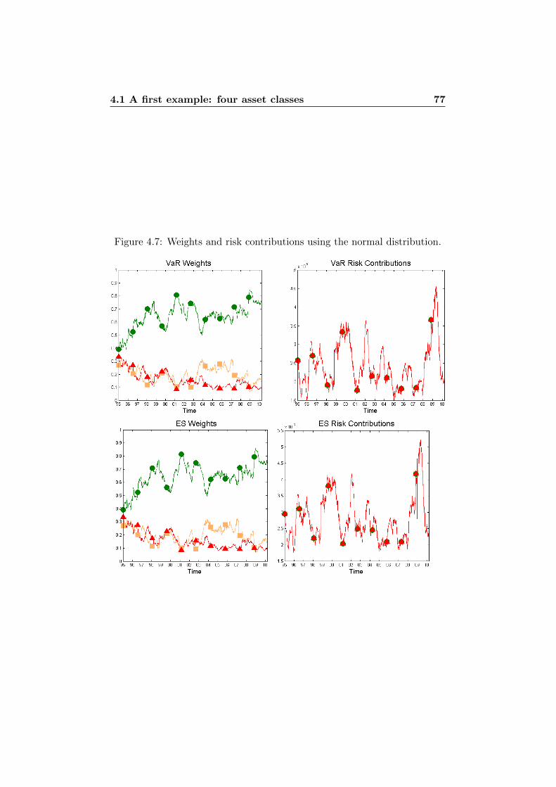
4.1 A first example: four asset classes 77
Figure 4.7: Weights and risk contributions using the normal distribution.
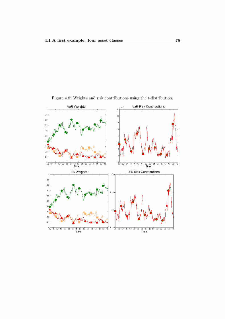
4.1 A first example: four asset classes 78
Figure 4.8: Weights and risk contributions using the t-distribution.
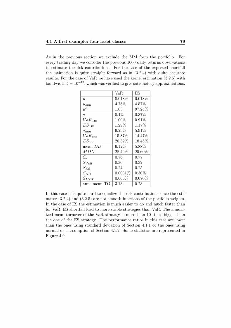
4.1 A first example: four asset classes 79
As in the previous section we exclude the MM form the portfolio. Forevery trading day we consider the previous 1000 daily returns observationsto estimate the risk contributions. For the case of the expected shortfallthe estimation is quite straight forward as in (3.2.4) with quite accurateresults. For the case of VaR we have used the kernel estimation (3.2.5) withbandwidth b = 10−12, which was verified to give satisfactory approximations.
VaR ES
µ 0.018% 0.018%µann 4.78% 4.57%µc 1.03 97.24%
σ 0.4% 0.37%V aR0.01 1.00% 0.91%ES0.01 1.29% 1.17%σann 6.29% 5.91%V aRann 15.87% 14.47%ESann 20.32% 18.45%
mean DD 6.12% 5.88%MDD 28.42% 25.60%
Sσ 0.76 0.77SV aR 0.30 0.32SES 0.24 0.25SDD 0.0031% 0.30%SMDD 0.066% 0.070%
ann. mean TO 3.13 0.23
In this case it is quite hard to equalize the risk contributions since the esti-mator (3.2.4) and (3.2.5) are not smooth functions of the portfolio weights.In the case of ES the estimation is much easier to do and much faster thanfor VaR. ES shortfall lead to more stable strategies than VaR. The annual-ized mean turnover of the VaR strategy is more than 10 times bigger thanthe one of the ES strategy. The performance ratios in this case are lowerthan the ones using standard deviation of Section 4.1.1 or the ones usingnormal or t assumption of Section 4.1.2. Some statistics are represented inFigure 4.9.
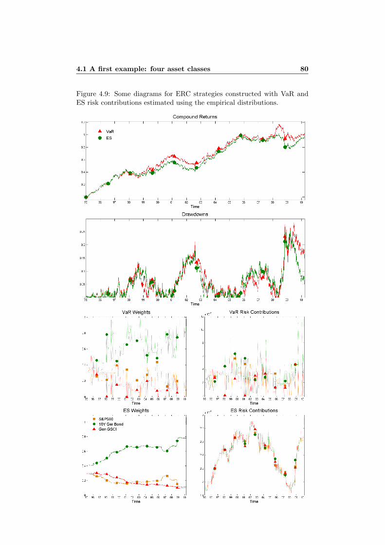
4.1 A first example: four asset classes 80
Figure 4.9: Some diagrams for ERC strategies constructed with VaR andES risk contributions estimated using the empirical distributions.

4.2 Stocks & Bonds Portfolios 81
4.2 Stocks & Bonds Portfolios
In this example we consider portfolios of USA/CH stocks and bonds over avery long period of more or less 77 years. We consider the period from Jan-uary 1931 to december 2008 using monthly observations and rebalancing theportfolio monthly. The stocks and bonds statistics for these two countriesfrom the 20s are the following.
S&P500 USA Bonds SPI CH Bonds
Mean 0.92% 0.47% 0.70% 0.37%
Ann. Mean 11.62% 5.85% 8.77% 4.54%
Max. 42.86% 14.35% 33.35% 9.62%
Min. -29.45% -9.22% -24.62% -3.57%
Standard deviation 5.53% 1.99% 4.74% 0.91%
Ann. standard deviation 19.17% 6.88% 16.43% 3.15%
Sharpe 0.61 0.85 0.53 1.44
Skewness 37.89% 97.12% 20.45% 92.46%
Kurtosis 12.75 10.28 7.84 16.67
The sample correlations are given by the following table.
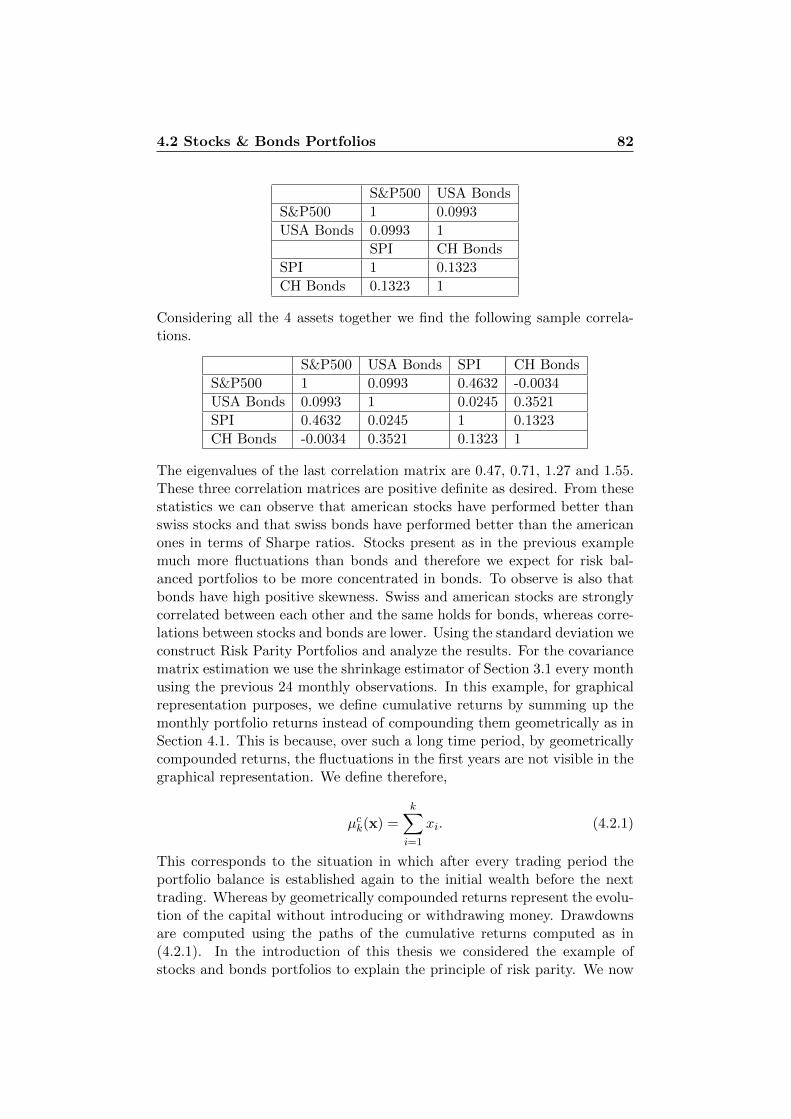
4.2 Stocks & Bonds Portfolios 82
S&P500 USA Bonds
S&P500 1 0.0993
USA Bonds 0.0993 1
SPI CH Bonds
SPI 1 0.1323
CH Bonds 0.1323 1
Considering all the 4 assets together we find the following sample correla-tions.
S&P500 USA Bonds SPI CH Bonds
S&P500 1 0.0993 0.4632 -0.0034
USA Bonds 0.0993 1 0.0245 0.3521
SPI 0.4632 0.0245 1 0.1323
CH Bonds -0.0034 0.3521 0.1323 1
The eigenvalues of the last correlation matrix are 0.47, 0.71, 1.27 and 1.55.These three correlation matrices are positive definite as desired. From thesestatistics we can observe that american stocks have performed better thanswiss stocks and that swiss bonds have performed better than the americanones in terms of Sharpe ratios. Stocks present as in the previous examplemuch more fluctuations than bonds and therefore we expect for risk bal-anced portfolios to be more concentrated in bonds. To observe is also thatbonds have high positive skewness. Swiss and american stocks are stronglycorrelated between each other and the same holds for bonds, whereas corre-lations between stocks and bonds are lower. Using the standard deviation weconstruct Risk Parity Portfolios and analyze the results. For the covariancematrix estimation we use the shrinkage estimator of Section 3.1 every monthusing the previous 24 monthly observations. In this example, for graphicalrepresentation purposes, we define cumulative returns by summing up themonthly portfolio returns instead of compounding them geometrically as inSection 4.1. This is because, over such a long time period, by geometricallycompounded returns, the fluctuations in the first years are not visible in thegraphical representation. We define therefore,
µck(x) =k∑i=1
xi. (4.2.1)
This corresponds to the situation in which after every trading period theportfolio balance is established again to the initial wealth before the nexttrading. Whereas by geometrically compounded returns represent the evolu-tion of the capital without introducing or withdrawing money. Drawdownsare computed using the paths of the cumulative returns computed as in(4.2.1). In the introduction of this thesis we considered the example ofstocks and bonds portfolios to explain the principle of risk parity. We now
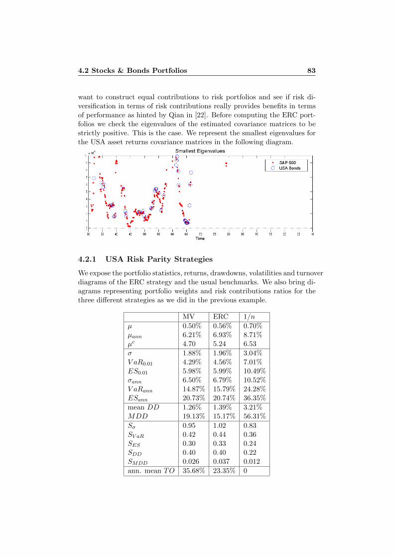
4.2 Stocks & Bonds Portfolios 83
want to construct equal contributions to risk portfolios and see if risk di-versification in terms of risk contributions really provides benefits in termsof performance as hinted by Qian in [22]. Before computing the ERC port-folios we check the eigenvalues of the estimated covariance matrices to bestrictly positive. This is the case. We represent the smallest eigenvalues forthe USA asset returns covariance matrices in the following diagram.
4.2.1 USA Risk Parity Strategies
We expose the portfolio statistics, returns, drawdowns, volatilities and turnoverdiagrams of the ERC strategy and the usual benchmarks. We also bring di-agrams representing portfolio weights and risk contributions ratios for thethree different strategies as we did in the previous example.
MV ERC 1/n
µ 0.50% 0.56% 0.70%µann 6.21% 6.93% 8.71%µc 4.70 5.24 6.53
σ 1.88% 1.96% 3.04%V aR0.01 4.29% 4.56% 7.01%ES0.01 5.98% 5.99% 10.49%σann 6.50% 6.79% 10.52%V aRann 14.87% 15.79% 24.28%ESann 20.73% 20.74% 36.35%
mean DD 1.26% 1.39% 3.21%MDD 19.13% 15.17% 56.31%
Sσ 0.95 1.02 0.83SV aR 0.42 0.44 0.36SES 0.30 0.33 0.24SDD 0.40 0.40 0.22SMDD 0.026 0.037 0.012
ann. mean TO 35.68% 23.35% 0
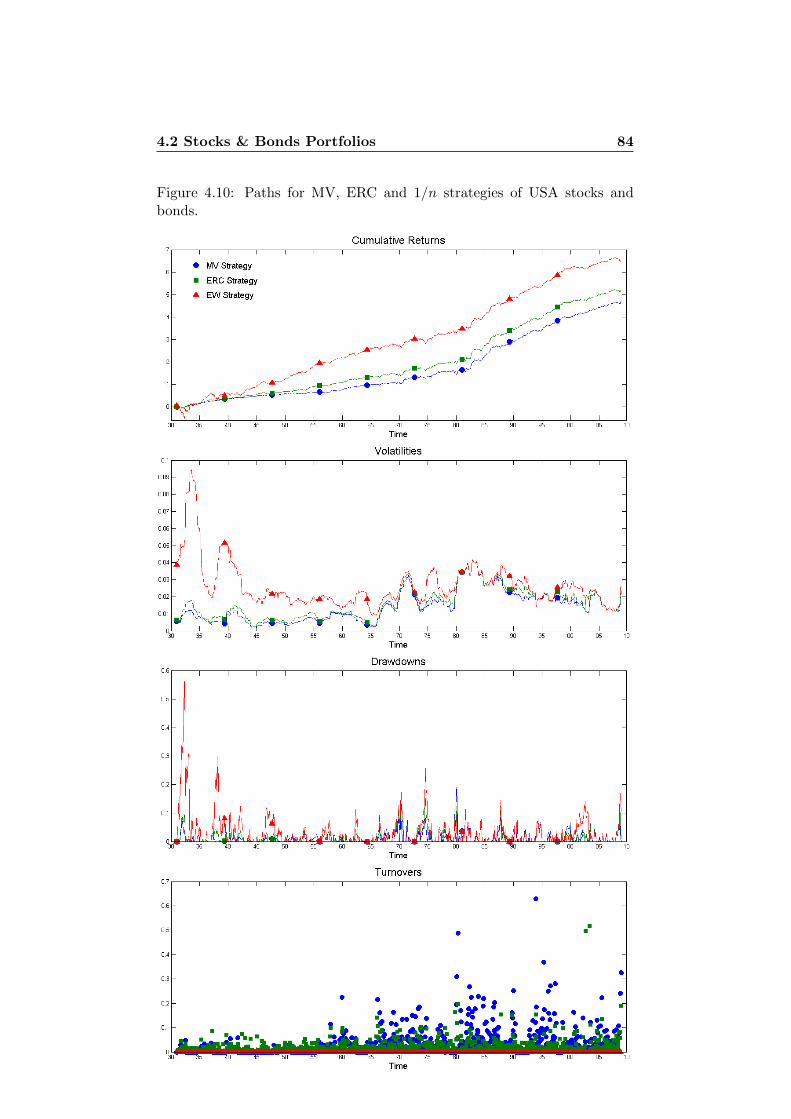
4.2 Stocks & Bonds Portfolios 84
Figure 4.10: Paths for MV, ERC and 1/n strategies of USA stocks andbonds.
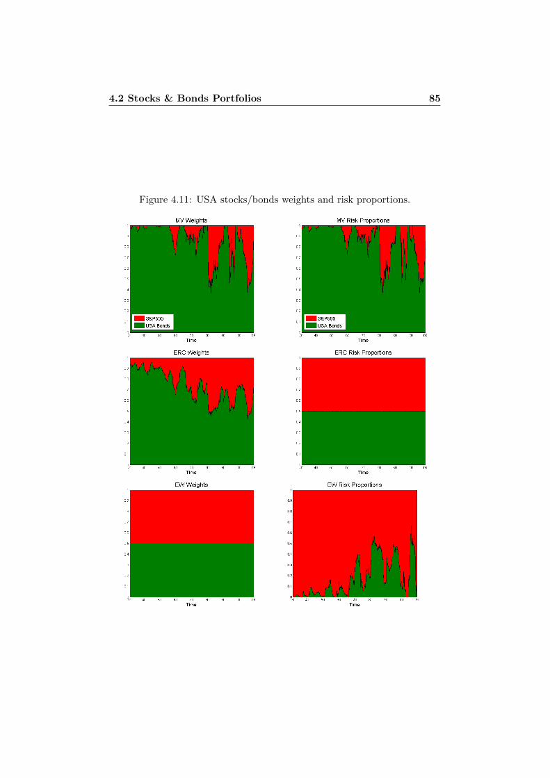
4.2 Stocks & Bonds Portfolios 85
Figure 4.11: USA stocks/bonds weights and risk proportions.
4.2 Stocks & Bonds Portfolios 86
The performance benefits in terms of Sharpe ratios that Qian [22] claimedto have observed are exactly visible also in this example. The Sharpe ratiosof USA stocks and bonds are respectively 0.61 and 0.85. The 50/50 strategyhas a Sharpe ratio of 0.83, which is smaller than the one of bonds andthis means that there is no benefit in splitting the wealth among stocks andbonds. This means that the EW strategy has poor diversification. The ERCstrategy provides higher Sharpe ratio than stocks and bonds individuallyand this represent the benefits of diversification. The Sharpe ratio of theMV portfolio is also higher than the ones of the assets. In particular wecan observe that ERC present the highest Sharpe ratio of 1.02 among thethree strategies. Performance ratios for the VaR and ES risk measures arealso better for the ERC strategy. It is important to observe that the 50/50strategy suffers from dramatic drawdowns compared with MV and ERC, MVhas the best mean drawdown and ERC has the best maximum drawdownover the whole period. A stable strategy in terms of drawdowns is veryimportant for asset management firms. Looking at the risk proportionsdiagrams we can observe that the risk contributions optimization has beenperformed successfully. The risk contributions are very precisely equalized.Interesting is to observe that by MV the risk proportion and the portfolioweights seem to be exactly equal. This is indeed true and can be easilyverified analytically. The MV portfolio minimizes the variance w′Ωw underthe constraint w′1 = 1, and hence must satisfy for i = 1, . . . , n and someLagrange multiplier λ
(Ωw)i − λ = 0. (4.2.2)
The risk proportions can be written as
RCi(w)√w′Ωw
=wi(Ωw)iw′Ωw
=λ
w′Ωwwi. (4.2.3)
Using the constraint it follows
1 =n∑i=1
RCi(w)√w′Ωw
=λ
w′Ωw
n∑i=1
wi =λ
w′Ωw, (4.2.4)
and hence combining the last two equations we see that for the strategy thatminimizes the variance the risk ratios must be the same as the portfolioweights. This suggests an alternative interpretation of how the strategyare constructed: by MV the risk is partitioned in the same way as thecapital, by ERC the risk is partitioned equally and by EW the capital ispartitioned equally. In terms of cumulative returns ERC is located betweenMV and EW, and the same holds for the volatility confirming the resultof Theorem 2.2.3. The ERC weights are stable in time, this is also verydesirable in practice, since high turnovers involve high transaction costs.The ERC portfolio exhibits a quite low turnover with an annualized mean

4.2 Stocks & Bonds Portfolios 87
of 23.35%. While ERC has high Sharpe ratio, it has lower return than EWbecause of the much lower volatility. An investor may therefore not be ableto achieve a certain return objective just by constructing a strategy withhigh Sharpe ratio. A possible way of dealing with low return is to leveragethe positions in order to achieve a higher level of return. For instance wecan leverage the ERC positions so that the ERC strategy has the same meanrate of return. This can be achieved using a leverage ratio of 1.247. In thisway we obtain a strategy with the same annualized mean return of 8.71% asthe EW strategy and an annualized volatility of 8.47%, lower than the oneof EW which is 10.52%. This reflects the fact that ERC has higher Sharperatio. Similarly, we can leverage the ERC positions such that the volatilityis the same. The required leverage for this is 1.5497. Using this leveragethe annualized mean return of ERC is 10.93%, which is better than EW,reflecting the higher Sharpe ratio of ERC.
4.2.2 CH Risk Parity Strategies
We do the same analysis for the swiss market.
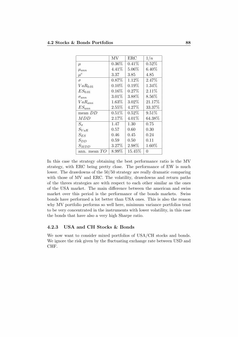
4.2 Stocks & Bonds Portfolios 88
MV ERC 1/n
µ 0.36% 0.41% 0.52%µann 4.41% 5.06% 6.40%µc 3.37 3.85 4.85
σ 0.87% 1.12% 2.47%V aR0.01 0.10% 0.19% 1.34%ES0.01 0.16% 0.27% 2.11%σann 3.01% 3.88% 8.56%V aRann 1.63% 3.02% 21.17%ESann 2.55% 4.27% 33.37%
mean DD 0.51% 0.52% 9.51%MDD 2.17% 4.01% 64.38%
Sσ 1.47 1.30 0.75SV aR 0.57 0.60 0.30SES 0.46 0.45 0.24SDD 0.59 0.50 0.11SMDD 3.27% 2.98% 1.60%
ann. mean TO 8.99% 15.45% 0
In this case the strategy obtaining the best performance ratio is the MVstrategy, with ERC being pretty close. The performance of EW is muchlower. The drawdowns of the 50/50 strategy are really dramatic comparingwith those of MV and ERC. The volatility, drawdowns and return pathsof the threes strategies are with respect to each other similar as the onesof the USA market. The main difference between the american and swissmarket over this period is the performance of the bonds markets. Swissbonds have performed a lot better than USA ones. This is also the reasonwhy MV portfolio performs so well here, minimum variance portfolios tendto be very concentrated in the instruments with lower volatility, in this casethe bonds that have also a very high Sharpe ratio.
4.2.3 USA and CH Stocks & Bonds
We now want to consider mixed portfolios of USA/CH stocks and bonds.We ignore the risk given by the fluctuating exchange rate between USD andCHF.
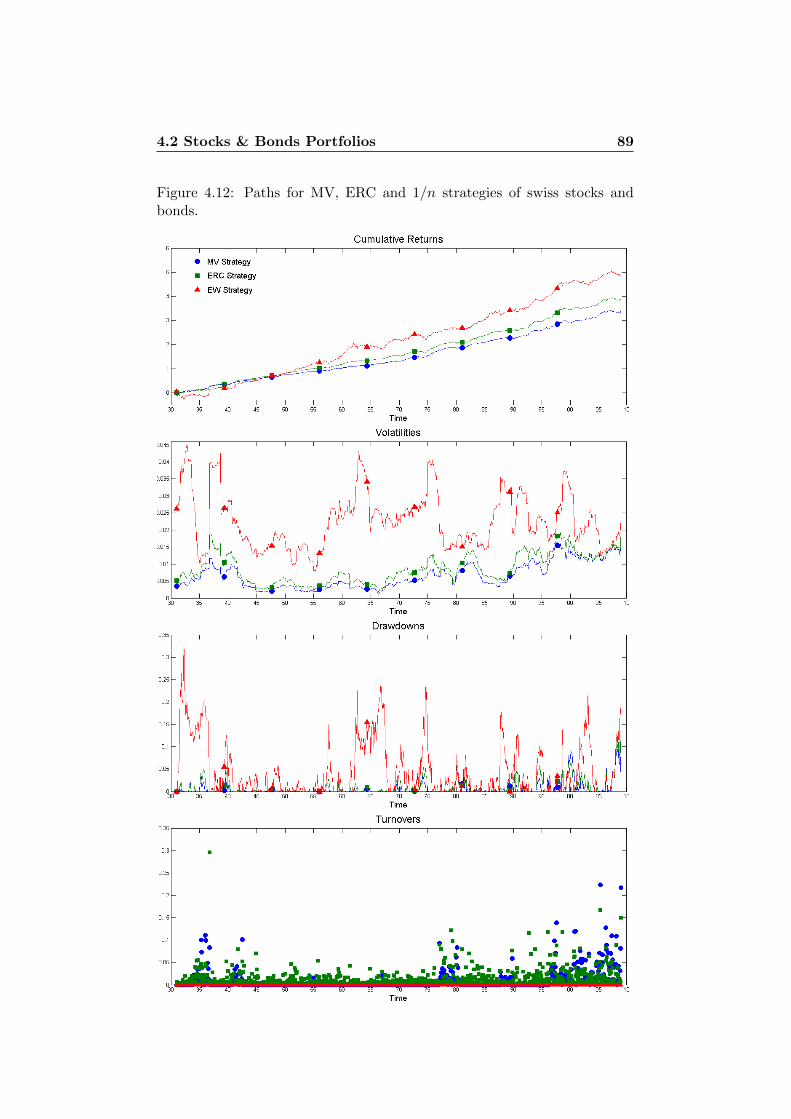
4.2 Stocks & Bonds Portfolios 89
Figure 4.12: Paths for MV, ERC and 1/n strategies of swiss stocks andbonds.
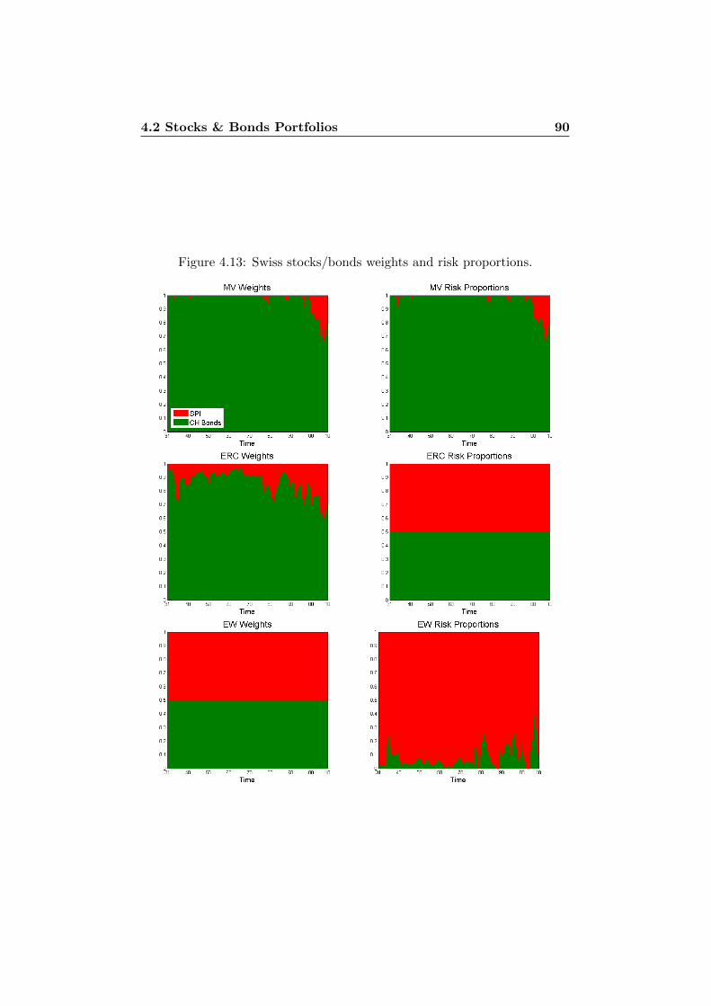
4.2 Stocks & Bonds Portfolios 90
Figure 4.13: Swiss stocks/bonds weights and risk proportions.
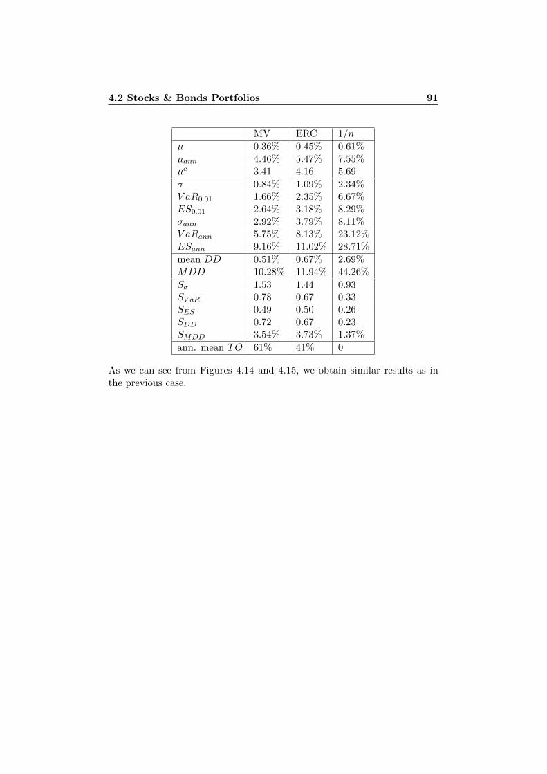
4.2 Stocks & Bonds Portfolios 91
MV ERC 1/n
µ 0.36% 0.45% 0.61%µann 4.46% 5.47% 7.55%µc 3.41 4.16 5.69
σ 0.84% 1.09% 2.34%V aR0.01 1.66% 2.35% 6.67%ES0.01 2.64% 3.18% 8.29%σann 2.92% 3.79% 8.11%V aRann 5.75% 8.13% 23.12%ESann 9.16% 11.02% 28.71%
mean DD 0.51% 0.67% 2.69%MDD 10.28% 11.94% 44.26%
Sσ 1.53 1.44 0.93SV aR 0.78 0.67 0.33SES 0.49 0.50 0.26SDD 0.72 0.67 0.23SMDD 3.54% 3.73% 1.37%
ann. mean TO 61% 41% 0
As we can see from Figures 4.14 and 4.15, we obtain similar results as inthe previous case.
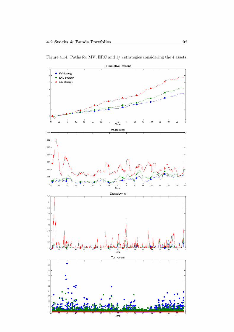
4.2 Stocks & Bonds Portfolios 92
Figure 4.14: Paths for MV, ERC and 1/n strategies considering the 4 assets.

4.2 Stocks & Bonds Portfolios 93
Figure 4.15: Weights and risk contributions of the 4 assets.

4.2 Stocks & Bonds Portfolios 94
4.2.4 Stability Considerations
We conclude this example comparing the results for USA ERC strategies us-ing different observation periods for the estimation of the covariance matrix.We consider 12, 24 and 60 observations.
12 24 60
µ 0.56% 0.56% 0.55%µann 6.89% 6.93% 6.82%µc 5.21 5.24 5.15
σ 1,97% 1.96% 1.98%V aR0.01 4.4% 4.56% 4.39%ES0.01 5.87% 5.99% 6.25%σann 6.81% 6.79% 6.87%V aRann 15.25% 15.79% 15.19%ESann 20.34% 20.74% 21.65%
mean DD 1.45% 1.39% 1.42%MDD 15.62% 15.17% 18.76%
Sσ 1.01 1.02 0.99SV aR 0.45 0.44 0.45SES 0.34 0.33 0.32SDD 0.38 0.40 0.39SMDD 3.56% 3.7% 2.94%
ann. mean TO 41.38% 23.35% 9.17%
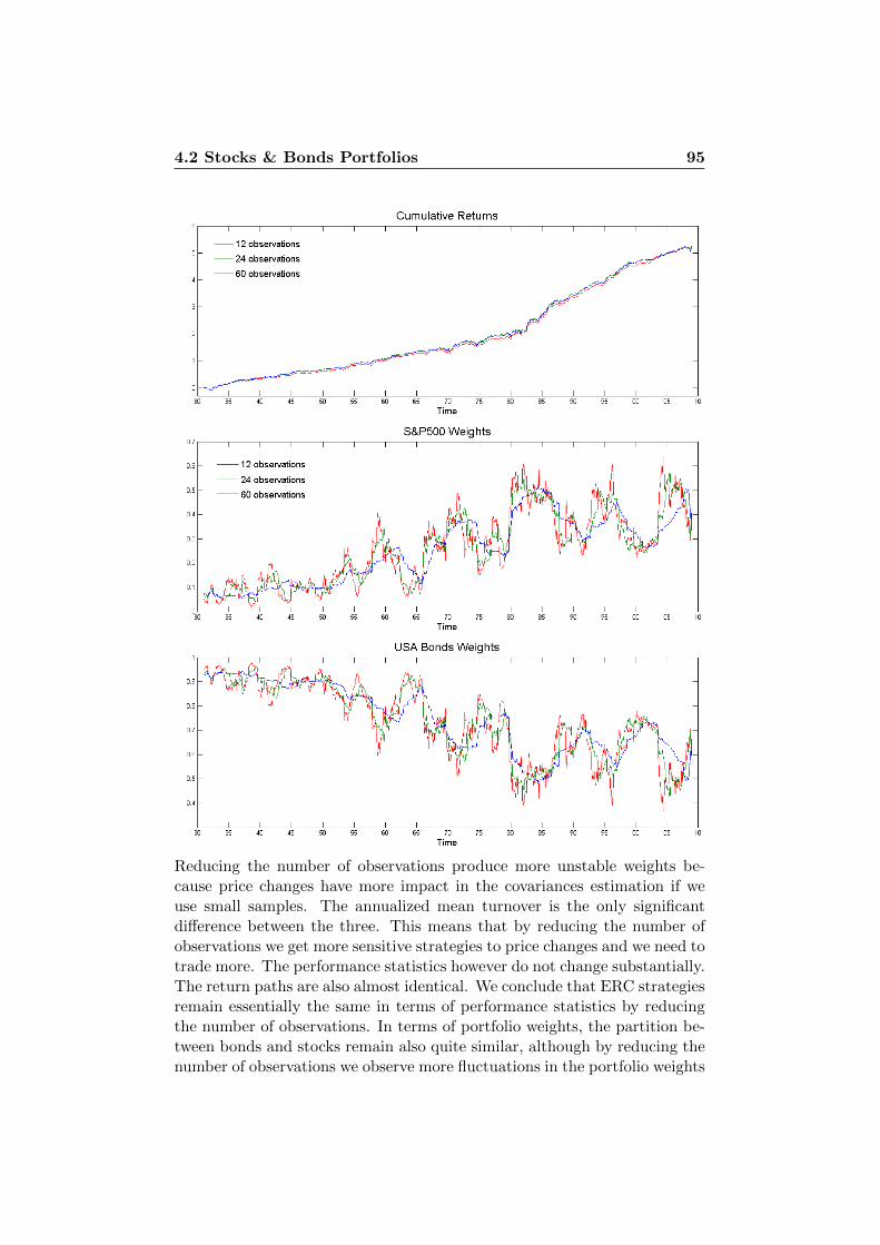
4.2 Stocks & Bonds Portfolios 95
Reducing the number of observations produce more unstable weights be-cause price changes have more impact in the covariances estimation if weuse small samples. The annualized mean turnover is the only significantdifference between the three. This means that by reducing the number ofobservations we get more sensitive strategies to price changes and we need totrade more. The performance statistics however do not change substantially.The return paths are also almost identical. We conclude that ERC strategiesremain essentially the same in terms of performance statistics by reducingthe number of observations. In terms of portfolio weights, the partition be-tween bonds and stocks remain also quite similar, although by reducing thenumber of observations we observe more fluctuations in the portfolio weights
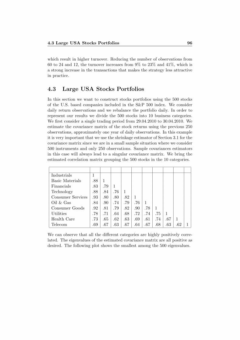
4.3 Large USA Stocks Portfolios 96
which result in higher turnover. Reducing the number of observations from60 to 24 and 12, the turnover increases from 9% to 23% and 41%, which isa strong increase in the transactions that makes the strategy less attractivein practice.
4.3 Large USA Stocks Portfolios
In this section we want to construct stocks portfolios using the 500 stocksof the U.S. based companies included in the S&P 500 index. We considerdaily return observations and we rebalance the portfolio daily. In order torepresent our results we divide the 500 stocks into 10 business categories.We first consider a single trading period from 29.04.2010 to 30.04.2010. Weestimate the covariance matrix of the stock returns using the previous 250observations, approximately one year of daily observations. In this exampleit is very important that we use the shrinkage estimator of Section 3.1 for thecovariance matrix since we are in a small sample situation where we consider500 instruments and only 250 observations. Sample covariances estimatorsin this case will always lead to a singular covariance matrix. We bring theestimated correlation matrix grouping the 500 stocks in the 10 categories.
Industrials 1Basic Materials .88 1Financials .83 .79 1Technology .88 .84 .76 1Consumer Services .93 .80 .80 .82 1Oil & Gas .84 .90 .74 .79 .76 1Consumer Goods .92 .81 .79 .82 .90 .78 1Utilities .78 .71 .64 .68 .72 .74 .75 1Health Care .73 .65 .62 .63 .69 .61 .74 .67 1Telecom .69 .67 .63 .67 .64 .67 .68 .63 .62 1
We can observe that all the different categories are highly positively corre-lated. The eigenvalues of the estimated covariance matrix are all positive asdesired. The following plot shows the smallest among the 500 eigenvalues.
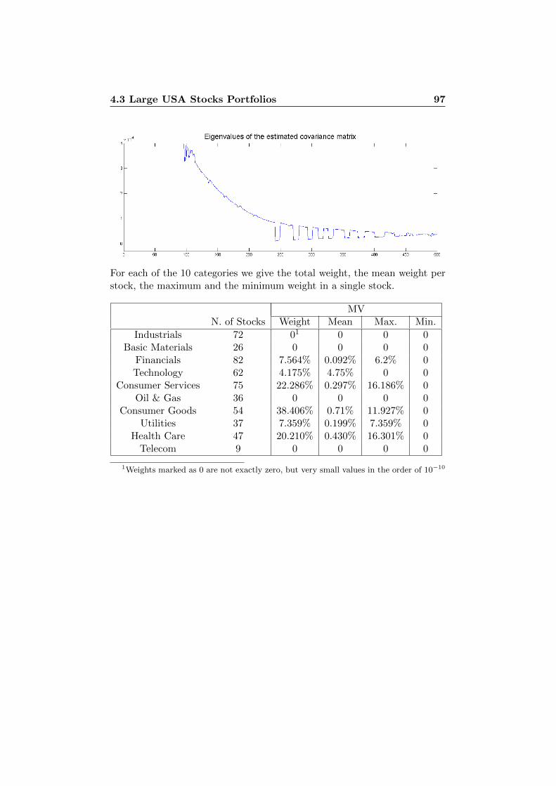
4.3 Large USA Stocks Portfolios 97
For each of the 10 categories we give the total weight, the mean weight perstock, the maximum and the minimum weight in a single stock.
MVN. of Stocks Weight Mean Max. Min.
Industrials 72 01 0 0 0Basic Materials 26 0 0 0 0
Financials 82 7.564% 0.092% 6.2% 0Technology 62 4.175% 4.75% 0 0
Consumer Services 75 22.286% 0.297% 16.186% 0Oil & Gas 36 0 0 0 0
Consumer Goods 54 38.406% 0.71% 11.927% 0Utilities 37 7.359% 0.199% 7.359% 0
Health Care 47 20.210% 0.430% 16.301% 0Telecom 9 0 0 0 0
1Weights marked as 0 are not exactly zero, but very small values in the order of 10−10

4.3 Large USA Stocks Portfolios 98
ERCWeight Mean Max. Min.
Industrials 13.007% 0.181% 0.298% 0.093%Basic Materials 3.649% 0.140% 0.261% 0.079%
Financials 11.858% 0.145% 0.337% 0.069%Technology 11.723% 0.189% 0.390% 0.097%
Consumer Services 15.284% 0.204% 0.552% 0.071%Oil & Gas 5.051% 0.140% 0.261% 0.094%
Consumer Goods 14.653% 0.271% 0.547% 0.093%Utilities 9.654% 0.261% 0.432% 0.109%
Health Care 12.853% 0.273% 0.486% 0.127%Telecom 2.269% 0.252% 0.386% 0.117%
EWWeight Mean Max. Min.
Industrials 14.400% 0.200% 0.200% 0.200%Basic Materials 5.200% 0.200% 0.200% 0.200%
Financials 16.400% 0.200% 0.200% 0.200%Technology 12.400% 0.200% 0.200% 0.200%
Consumer Services 15.000% 0.200% 0.200% 0.200%Oil & Gas 7.200% 0.200% 0.200% 0.200%
Consumer Goods 10.800% 0.200% 0.200% 0.200%Utilities 7.400% 0.200% 0.200% 0.200%
Health Care 9.400% 0.200% 0.200% 0.200%Telecom 1.800% 0.200% 0.200% 0.200%
MV portfolios are typically very concentrated and this can be observed veryclearly in this example. Using the MV strategy we invest in only 5 categoriesand looking at maximal weights in each category we can deduce that morethen 50% of our wealth is invested in only 5 stocks out of 500. In thisexample the ERC portfolio is much more homogeneous than in the twoprevious examples. This is because we are considering instruments thatcontribute to the total portfolio risk similarly with respect to each others.We can observe that the optimization can be performed very accuratelyalso in this case where we minimize a function of 500 variables. However,the optimization using the Matlab function fmincon takes quite a lot oftime for this problem. For example, to obtain accurate equalization of riskcontributions in the above one period example my Matlab implementationneeded approximately 140 seconds on my machine and this means that ifwe want to backtest the strategy for the previous 10 years we will needapproximately 4 days. For this reason I am going to consider only the periodfrom 01.01.2009 to 29.04.2010 to compare the ERC strategy with the equallyweighted strategy. For every trading period we compute the eigenvaluesof the estimated covariance matrices, and in order to verify that all theeigenvalues are positive we plot the minimal eigenvalue for each period.
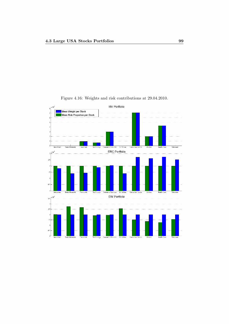
4.3 Large USA Stocks Portfolios 99
Figure 4.16: Weights and risk contributions at 29.04.2010.

4.3 Large USA Stocks Portfolios 100
The portfolios statistics over this short period are similar comparing the twostrategies (except for the turnover). This is because the set of instrumentsis very homogeneous.
ERC 1/n
µ 0.14% 0.17%µann 40.35% 51.53%µc 53.29% 67.37%
σ 1.56% 1.87%V aR0.01 4.68% 5.43%ES0.01 5.13% 5.96%σann 24.68% 29.57%V aRann 73.98% 85.83%ESann 81.09% 94.22%
mean DD 4.14% 5.01%MDD 28.46% 31.88%
Sσ 1.64 1.74SV aR 0.55 0.6SES 0.50 0.55SDD 3.27% 3.32%SMDD 0.48% 0.52%
ann. mean TO 1.52 0.58%

4.3 Large USA Stocks Portfolios 101
Figure 4.17: Paths for the ERC and 1/n strategies.

Chapter 5
Diversification Analysis
From a qualitative point of view the concept of diversification is quite clear:a portfolio is well-diversified if shocks in the individual components do notheavily impact on the overall portfolio. However, as Meucci [19] has noticed,there is no broadly accepted precise and quantitative definition of diversi-fication. In this thesis we have considered diversification in terms of riskcontributions of the individual assets. We have shown in Chapter 1 that asuitable definition of risk contribution can be obtained considering partialderivatives of the risk measure with respect to the portfolio components.We then constructed portfolio equalizing these risk contributions. In thischapter we want to present following [19] some methodologies to quantifydiversification and apply them to one of the numerical examples of Chapter4.
5.1 Diversification Measures
Consider as in the previous chapters n investment opportunities and denoteby w ∈ Rn a vector of portfolio weights satisfying the budget constraint1′w = l. We consider the volatility ρ(w) =
√w′Ωw as the measure of
portfolio risk. As in the previous chapters Ω ∈ Rn×n denotes the covari-ance matrix of the assets returns. There are many naive ways of definingdiversification measures in terms of portfolio weights:
DHer = 1−w′w,
DBP = −n∑i=1
wi log(wi),
DγHK = −
(n∑i=1
wγi
) 1γ−1
, γ > 0.
(5.1.1)
The first is known as Herfindal index. It is easy to see that it is zero for
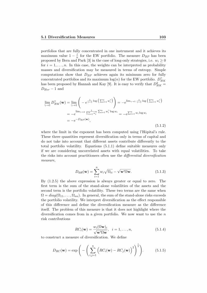
5.1 Diversification Measures 103
portfolios that are fully concentrated in one instrument and it achieves itsmaximum value 1 − l
n for the EW portfolio. The measure DBP has beenproposed by Bera and Park [3] in the case of long-only strategies, i.e. wi ≥ 0for i = 1, . . . , n. In this case, the weights can be interpreted as probabilitymasses and diversification may be measured in terms of entropy. Simplecomputations show that DBP achieves again its minimum zero for fullyconcentrated portfolios and its maximum log(n) for the EW portfolio. Dγ
HK
has been proposed by Hannah and Kay [9]. It is easy to verify that D2HK =
DHer − 1 and
limγ→1
DγHK(w) = lim
γ→1
(− e
1γ−1
log(∑n
i=1 wγi
))= −elimγ→1
1γ−1
log(∑n
i=1 wγi
)= −e
limγ→11∑n
i=1wγi
∑ni=1 w
γi logwi
= −e∑ni=1 wi logwi
= −e−DBP (w),
(5.1.2)
where the limit in the exponent has been computed using l’Hopital’s rule.These three quantities represent diversification only in terms of capital anddo not take into account that different assets contribute differently to thetotal portfolio volatility. Equations (5.1.1) define suitable measures onlyif we are considering uncorrelated assets with equal volatilities. To takethe risks into account practitioners often use the differential diversificationmeasure,
Ddiff(w) =
n∑i=1
wi√
Ωii −√
w′Ωw. (5.1.3)
By (1.2.5) the above expression is always greater or equal to zero. Thefirst term is the sum of the stand-alone volatilities of the assets and thesecond term is the portfolio volatility. These two terms are the same whenΩ = diag(Ω11, . . . ,Ωnn). In general, the sum of the stand-alone risks exceedsthe portfolio volatility. We interpret diversification as the effect responsibleof this difference and define the diversification measure as the differenceitself. The problem of this measure is that it does not highlight where thediversification comes from in a given portfolio. We now want to use the nrisk contributions
RCi(w) =wi(Ωw)i√
w′Ωw, i = 1, . . . , n, (5.1.4)
to construct a measure of diversification. We define
DRC(w) = exp
(−
(n∑
i,j=1
(RCi(w)−RCj(w)
)2) 1
2). (5.1.5)
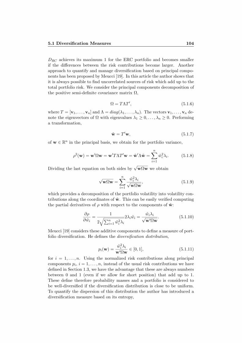
5.1 Diversification Measures 104
DRC achieves its maximum 1 for the ERC portfolio and becomes smallerif the differences between the risk contributions become larger. Anotherapproach to quantify and manage diversification based on principal compo-nents has been proposed by Meucci [19]. In this article the author shows thatit is always possible to find uncorrelated sources of risk which add up to thetotal portfolio risk. We consider the principal components decomposition ofthe positive semi-definite covariance matrix Ω,
Ω = TΛT ′, (5.1.6)
where T = [v1, . . . ,vn] and Λ = diag(λ1, . . . , λn). The vectors v1, . . . ,vn de-note the eigenvectors of Ω with eigenvalues λ1 ≥ 0, . . . , λn ≥ 0. Performinga transformation,
w = T ′w, (5.1.7)
of w ∈ Rn in the principal basis, we obtain for the portfolio variance,
ρ2(w) = w′Ωw = w′TΛT ′w = w′Λw =
n∑i=1
w2i λi. (5.1.8)
Dividing the last equation on both sides by√
wΩw we obtain
√wΩw =
n∑i=1
w2i λi√
wΩw, (5.1.9)
which provides a decomposition of the portfolio volatility into volatility con-tributions along the coordinates of w. This can be easily verified computingthe partial derivatives of ρ with respect to the components of w:
∂ρ
∂wi=
1
2√∑n
i=1 w2i λi
2λiwi =wiλi√w′Ωw
. (5.1.10)
Meucci [19] considers these additive components to define a measure of port-folio diversification. He defines the diversification distribution,
pi(w) =w2i λi
w′Ωw∈ [0, 1], (5.1.11)
for i = 1, . . . , n. Using the normalized risk contributions along principalcomponents pi, i = 1, . . . , n, instead of the usual risk contributions we havedefined in Section 1.3, we have the advantage that these are always numbersbetween 0 and 1 (even if we allow for short position) that add up to 1.These define therefore probability masses and a portfolio is considered tobe well-diversified if the diversification distribution is close to be uniform.To quantify the dispersion of this distribution the author has introduced adiversification measure based on its entropy,
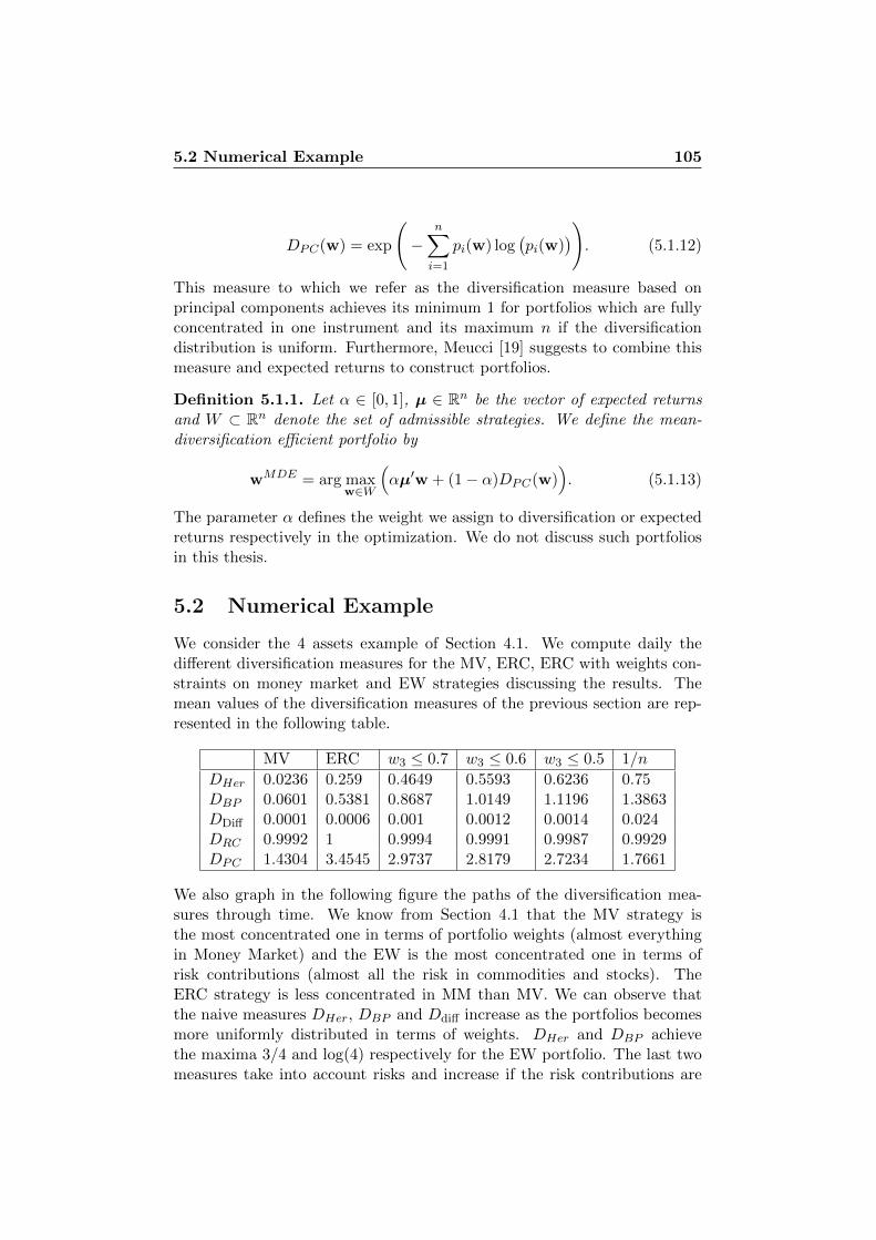
5.2 Numerical Example 105
DPC(w) = exp
(−
n∑i=1
pi(w) log(pi(w)
)). (5.1.12)
This measure to which we refer as the diversification measure based onprincipal components achieves its minimum 1 for portfolios which are fullyconcentrated in one instrument and its maximum n if the diversificationdistribution is uniform. Furthermore, Meucci [19] suggests to combine thismeasure and expected returns to construct portfolios.
Definition 5.1.1. Let α ∈ [0, 1], µ ∈ Rn be the vector of expected returnsand W ⊂ Rn denote the set of admissible strategies. We define the mean-diversification efficient portfolio by
wMDE = arg maxw∈W
(αµ′w + (1− α)DPC(w)
). (5.1.13)
The parameter α defines the weight we assign to diversification or expectedreturns respectively in the optimization. We do not discuss such portfoliosin this thesis.
5.2 Numerical Example
We consider the 4 assets example of Section 4.1. We compute daily thedifferent diversification measures for the MV, ERC, ERC with weights con-straints on money market and EW strategies discussing the results. Themean values of the diversification measures of the previous section are rep-resented in the following table.
MV ERC w3 ≤ 0.7 w3 ≤ 0.6 w3 ≤ 0.5 1/n
DHer 0.0236 0.259 0.4649 0.5593 0.6236 0.75DBP 0.0601 0.5381 0.8687 1.0149 1.1196 1.3863DDiff 0.0001 0.0006 0.001 0.0012 0.0014 0.024DRC 0.9992 1 0.9994 0.9991 0.9987 0.9929DPC 1.4304 3.4545 2.9737 2.8179 2.7234 1.7661
We also graph in the following figure the paths of the diversification mea-sures through time. We know from Section 4.1 that the MV strategy isthe most concentrated one in terms of portfolio weights (almost everythingin Money Market) and the EW is the most concentrated one in terms ofrisk contributions (almost all the risk in commodities and stocks). TheERC strategy is less concentrated in MM than MV. We can observe thatthe naive measures DHer, DBP and Ddiff increase as the portfolios becomesmore uniformly distributed in terms of weights. DHer and DBP achievethe maxima 3/4 and log(4) respectively for the EW portfolio. The last twomeasures take into account risks and increase if the risk contributions are
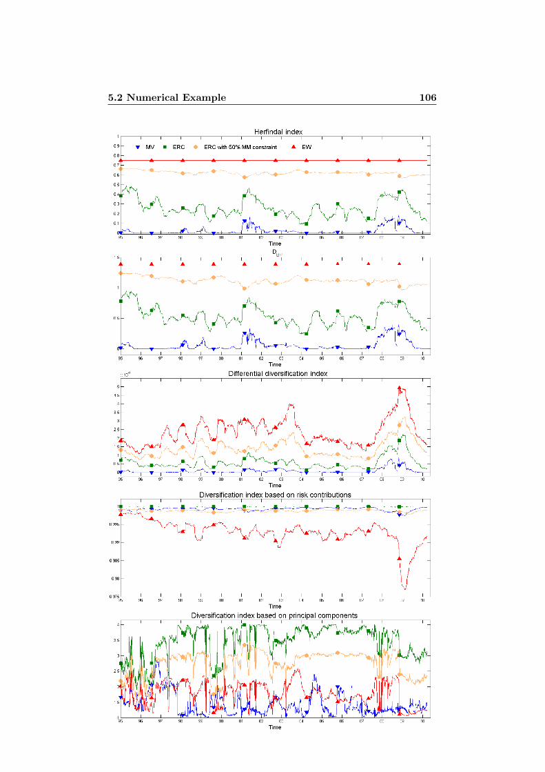
5.2 Numerical Example 106

5.2 Numerical Example 107
equalized. This was already clear from the definition for the measure DRC .It is however interesting to observe that the same holds for the measure DPC
which is not based on the risk contributions with respect to which we areoptimizing in the ERC approach. The maximum value of this measure forthis example is 4 and this value is sometimes reached by the ERC optimalportfolio. This means that in some cases the optimal portfolio with respectto DRC coincides with the one with respect to DPC .
Conclusion
In this thesis we have discussed in detail how risk parity portfolios are con-structed and we have performed some valuations based on historical data.In conclusion, we would like to explain the limitations of this approach thatbecome evident from the numerical results of Chapter 4. We also want tobring in some ideas for further developments of this material.We have already indicated in Chapter 2 that nothing prevents us from apply-ing this methodology using other risk measures than the standard deviation(for example Value-at-Risk or Expected Shortfall). In practice however,using other risk measures than the volatility becomes difficult.In Section 4.1 we have first considered this issue using two elliptical modelsfor the asset returns (normally and t-distributed returns). In this case, wehave analytical expressions for the risk contributions in terms of the assetreturns covariances and expected values. This fact allowed us to easilycompute equal contributions to risk portfolios using a shrinkage estimatorfor the covariance matrix (see Chapter 3). No significant difference in theallocation and performance has been observed in that example with respectto the allocation obtained using the volatility. Elliptical distributions donot always provide a good model for asset returns, especially in the case ofinstruments that exhibit high skewness. Generally, estimating the expectedreturns using the sample estimator leads to more unstable strategies. Wehave restricted ourselves to two special cases of elliptical models, but it wouldbe also interesting to start with a completely general elliptical model and tryto fit the parameters. The analytical expressions for the risk contributionsin a general elliptical setting are known and given in Theorem 1.4.3. Thequantities µ, Ω and ρ(Y1) need to be estimated. Some estimation methodsare available for the expected returns µ and the dispersion matrix Ω, see forexample [17] Section 3.2.4. The quantity ρ(Y1) depends on the underlyingspherical distribution. Empirical data for Y may be obtained from datafor X computing Ω−1/2(X − µ), where Ω1/2 is the Cholesky factor of Ω.Estimating risk contributions in a general elliptical framework may lead tomore accurate results than using a multivariate t-distribution as model forthe asset returns.In Chapter 3 we have also presented some classical estimators of VaR andES risk contributions using empirical distributions. These approximations

109
are however quite rough and, as we have observed in Section 4.1.3, they leadto unstable portfolios (especially for VaR) with a lower performance thanthe other ones.For these reasons and from our numerical experiments we conclude thatthe ERC approach can most easily and efficiently be implemented for thevolatility. First of all, no particular distribution assumption is needed. Sec-ondly, we are only required to estimate the variances and covariances forwhich a solid estimator has been discussed in Chapter 3. Moreover, as wehave verified in Section 4.2, the portfolio weights and the performances arestable with respect to the covariance matrix estimation. From our numericalresults it is also clear that the minimum variance portfolio is in most circum-stances not applicable because of its extremely concentrated exposures (seefor example Section 4.3), and that ERC portfolios are an efficient trade-offbetween 1/n and MV strategies.Despite these nice properties of equal volatility contributions, it is importantto realize that volatility is not the same as risk and it is not the only thingwe need to know about the portfolio. Levels of volatilities that might appearunder control may result in high losses, which may force the investors to cutdown their exposures. For example, if we consider the 4 assets example ofSection 4.1, we observe that the annualized volatility of the ERC strategyis 1.12%. In order to magnify the returns you may leverage the portfolioup to 8.16%, obtaining the same volatility as the equally weighted portfolio.This would lead to a maximum drawdown for the strategy of 29.22% in theperiod 2008-2009. The observed maximum drawdown in the same periodfor the 1/n portfolio is 64.38%. It is therefore important to realize that theportfolio volatility is not telling us everything about the potential losses,but other risk indicators need to be considered, especially when investorsare amplifying returns using leverage. The use of leverage allows investorsto reach higher returns, but at the same time leveraged investors may notbe able to wait for prices to reach reasonable levels. Another problematicissue about leveraging positions is that the risks the investors are leveragingmay not actually have positive return associated with them. Stocks andbonds allow the issuers to acquire the capital they need to function, andfor this capital the issuers promise to the investors a positive return bytaking on volatility. The situation looks different for commodities futures,for these types of contracts we have a buyer and a seller, and at the expirydate the contract will cease to exist. Why should the buyer be entitled to asystematically positive return and why should the commodity futures sellerbe prepared to accept a systematically negative return? The profits andlosses are symmetrical to the buyer and the seller since both of them aretaking on volatility, and where there is a winner, there is always also a loser.Asset classes without positive risk premiums associated with them are notsuitable for long-term returns and leveraged positions in these assets shouldnot be taken.
110
The use of volatility in Chapter 4 is also questionable since some of the assetclasses under consideration have high negative skewness. See for examplebonds and commodities futures in Section 4.1. Negative skewness meansthat the negative returns tend to be larger in magnitude than the positiveones. In this case the volatility is not able to capture what the true downsiderisk is. This is particularly pronounced in the context of credit risks. Theborrower will either pay back the loan or default, in case he pays back theloan, the return is slightly positive, in case he doesn’t pay back the loan thereturn is strongly negative. It is impossible to quantify precisely the risk inthis case for a given period of observations by simply estimating volatilitycontributions. Combining the unknown risks of the investment with leveragecan be very dangerous.In Section 4.3 we have constructed risk parity portfolios for assets of thesame risk class (500 stocks). In this situation where the risk is very ho-mogeneously distributed among the assets there is no significant differencebetween balancing risks and splitting the wealth equally among the assets.The results are represented in Figures 4.15 and 4.16. The performanceremains very similar (even lower) and the ERC approach requires a muchhigher turnover than the equally weighted allocation. We conclude thereforethat in such a situation it is not worth to switch from 1/n to risk balancedallocations.There are of course many improvement that can be done to the topics dis-cussed in this thesis. In Chapter 3 we limited ourselves only to the estimationof risk contributions using historical data. Methods based on Monte-Carlosimulations may also be developed. In order to apply the ERC principle tomore appropriate risk measures such as Expected Shortfall or Semi-Variance,more sophisticated techniques to estimate the risk contributions need to bediscussed. Some more accurate techniques for Value-at-Risk and ExpectedShortfall can be found in [20].In Chapter 5, we have introduced a different notion of risk contributionsbased on the principal components of the covariance matrix and we haveseen that these contributions correspond exactly to the partial derivatives ofthe volatility along the principal components. We haven’t tried to computethe optimal portfolio maximizing the measure DPC instead of DRC . InSection 5.2, we have observed computing DPC for the portfolios of Section4.1 that ERC portfolios tend to have high diversification values in terms ofDPC as well and that in some cases they exhibit values that are pretty closeto the maximum. This happens when the covariance matrix is very close tobe diagonal, but in general the two allocations differ. It would be interestingto compare the allocation and the performance of the two principles in someexamples.In Section 4.1 we have considered weights constraints in the Money Mar-ket and observed higher returns without affecting significantly the perfor-mance ratios (for some constraints we have even observed slightly higher
111
performance ratios). This motivates the following question: how can we de-viate from the ERC diversified portfolio in order to increase performance?Meucci [19] has proposed the mean-diversification efficient portfolio (Def-inition 5.1.1). Using this selection criterion we deviate from the perfectlydiversified portfolio (diversification measured using principal components asexplained in Section 5.1) incorporating expected returns information.From our numerical results and considering the above remarks we concludethat the ERC approach for the volatility as risk measure provides an inter-esting benchmark, based only on risk diversification, that has some limita-tions but also some advantages: it is based on a quite simple mathematicalframework, it can be easily implemented having an efficient optimizationsolver (such as in Matlab), it provides higher performance ratios than thetraditional equally weighted allocation, and it is based on a quite intuitiveprinciple that can also be explained effortless to people without a mathe-matical background in portfolio construction.
Appendix A
Spherical and EllipticalDistributions
We introduce formally and present the basic properties of this importantclass of multivariate distributions. We begin with the special case of spher-ical distributed random variables.
Definition A.1. A random vector R = (R1, . . . , Rn) has spherical dis-tribution if, for every orthogonal map U ∈ Rn×n (i.e. a map satisfyingU ′U = UU ′ = In) it holds
UR(d)∼ R, (A.1)
i.e. spherically distributed random variables are those with invariant distri-bution under orthogonal transformations.
The following theorem provides the main ways of characterizing sphericaldistributions.
Theorem A.1. The following statements are equivalent.
1. R is spherically distributed.
2. The characteristic function of R satisfies, for any t ∈ Rn, φR(t) =E[eit
′R] = ψ(t′t) for some scalar function ψ.
3. For every a ∈ Rn, it holds a′R(d)∼ |a|R1, where | · | denotes the Eu-
clidean norm.
Property 2 tells us that the distribution of a spherical random variable iscompletely described by a scalar function ψ. We introduce therefore thenotation R ∼ Sn(ψ), for spherical distributed random variables. Property3 is very important and has been used in Theorem 1.2.1. It allows to char-acterize linear combinations of spherical random vectors. The proof of this
113
result can be found in [17] Theorem 3.19. It can be easily verified using [17]Theorem 3.22 that, for R ∼ S(ψ), E[R] = 0 and that the covariance matrix(if the second moments are finite) is given by Ω = c(ψ)In where c(ψ) > 0 isa positive constant.
Example A.1. Consider a random vector R ∈ N (0, In) with the stan-dard uncorrelated multinormal distribution. R is clearly spherical, since itscharacteristic function is given by
φR(t) = E[eit′R] = ψ(t′t) (A.2)
with ψ(x) = e−12x. We can see spherical distributions as an extension of
standard multinormal distributions N (0, In).The reason why we introducethis generalization is that these distributions allow to describe heavy tails.
In Example 1.1.4 we describe a model based on the t-distribution which isalso a spherical distribution. Elliptical distributions are affine transforma-tion of spherical distributions.
Definition A.2. R has an elliptical distribution if
R(d)∼ AY + µ (A.3)
where Y ∈ Sk(ψ), A ∈ Rn×k and µ ∈ Rn.
The characteristic function of an elliptical distributed random variable isgiven by
φR(t) = E[eit′(AY+µ)
]= eit
′µE[ei(A
′t)′Y]
= eit′µψ(t′Ωt) (A.4)
where Ω = A′A. The distribution of an elliptical distributed random vari-able is therefore determined by the parameters µ, called the location vector,Ω, referred to as dispersion matrix, and the function ψ, the characteristicgenerator of the corresponding spherical distribution. We use the notationR ∼ En(µ,Ω, ψ). Note that Ω and ψ are not uniquely determined by the dis-tribution, but only up to a positive constant (consider the pair (cΩ, ψ(·/c))for c > 0). For elliptical distributed random variables we have E[R] = µand, provided second moments exist, its covariance matrix is a multiple ofΩ. It is therefore possible to find an elliptical representation En(µ,Ω, ψ) sothat Ω is the covariance matrix of R. However we do not impose this withthe above notation. We now look at some basic properties of this class ofrandom variables. If we take linear combinations of elliptical random vec-tors these remain elliptical: let R ∼ En(µ,Ω, ψ) and for any B ∈ Rk×n andb ∈ Rn, we have
BR + b ∼ En(Bµ + b, B′ΩB,ψ). (A.5)

114
Particularly important in our case is the fact that m′R ∼ En(m′µ,m′Ωm, ψ).From this it follows that marginal distributions of R must be also ellipticaldistributions: separate the coordinates of the random vector according toR = (R(l),R(n−l)), where R(l) is the vector of the first l coordinates andR(n−k)) is the vector of the remaining coordinates, then we have
R(l) ∼ El(µ(l),Ω(l), ψ), R(n−l) ∼ En−l(µ(n−l),Ω(n−l), ψ) (A.6)
where µ = (µ(l),µ(n−l)), Ω(l) ∈ Rl×l and Ω(n−l) ∈ R(n−l)×(n−l) are thecorresponding sub vectors/matrices.
Appendix B
Inequality Constraints andKuhn-Tucker Conditions
We are interested in minimizing a function in several variables under someequality and possibly also inequality constraints. Formally the problem isthe following,
minx∈Rn
f(x) subject to
ci(x) = 0 i ∈ Eci(x) ≥ 0 i ∈ I
, (B.1)
where f and ci are continuously differentiable functions on Rn, and E andI are two finite set of indices that correspond to the equality and inequalityconstraints respectively. We define by F = x ∈ Rn|ci(x) = 0 for all i ∈E , ci(x) ≥ 0 for all i ∈ I the set of all feasible vectors. We want to restrictourselves to vectors satisfying certain constraints qualifications.
Definition B.1. The active set A(x) at any feasible x ∈ F is defined as
A(x) = E ∪ i ∈ I : ci(x) = 0, (B.2)
i.e. it consists of the equality constraints indices together with the indices ofthe inequality constraints where equality is reached.
Definition B.2. Given a vector x and the corresponding active set A(x) wesay that the linear independence constraint qualification, abbreviated LICQ,holds if the gradients
∇ci(x) for i ∈ A(x) (B.3)
are linearly independent.
The following first order conditions are the foundation of the most popularalgorithms to solve (B.1), in the literature people usually refer to them asKuhn-Tucker conditions. A vector x∗ is called a local solution of (B.1) if
116
x∗ ∈ F and there is a neighborhood N of x∗ such that f(x) ≥ f(x∗) for allx ∈ N ∩ F .
Theorem B.0.1. Define the Lagrange function for the minimization prob-lem (B.1) as
L(x,λ) = f(x)−∑i∈E∪I
λici(x). (B.4)
Suppose that x∗ is a local solution of (B.1) and that the LICQ holds atx∗. Then, there is a Lagrange multiplier vector λ∗, with components λ∗i ,i ∈ E ∪ I, such that the following conditions are satisfied at (x∗,λ∗)
∇xL(x∗,λ∗) = 0,
ci(x∗) = 0, for all i ∈ E ,
ci(x∗) ≥ 0, for all i ∈ I,
λ∗ ≥ 0, for all i ∈ I,λ∗ci(x
∗) = 0, for all i ∈ E ∪ I.
(B.5)
The proof of this theorem is quite complex and can be found in [21] Section12.4.
Appendix C
Sequential QuadraticProgramming
As we have seen in Chapter 2 in order to find optimal portfolio strategieswe need to solve numerical minimization problems of the form (B.1). Wenow discuss one efficient method to do this which is implemented in Mat-lab under the function fmincon that minimizes general functions of severalvariables under general constraints. It is important to understand at leastqualitatively how this function works since it is the source of all our numer-ical results presented in Chapter 4. It is important to note that there arethree different algorithms used by this function, and the one we are going touse and discuss here is the one referred to as active-set algorithm in the de-scription of the function available in the Matlab Product Help. This methodtries to compute the Lagrange multipliers from the Kuhn-Tucker conditions(B.5) explicitly by solving in every iteration a quadratic programming sub-problem. These types of methods are usually referred to in the literatureas sequential quadratic programming methods, abbreviated SQP methods.We want to sketch the idea used by SQP algorithms, explaining very brieflyhow it is implemented in the Matlab function we have used in Chapter 4.Complete description about how to construct QP and SQP algorithms canbe found in [21] Chapter 16 and Chapter 18. We begin considering onlyequality constraints. The method consists mainly in deriving an appro-priate QP subproblem. This can found applying the Newton’s method fornon-linear equations to the Kuhn-Tucker conditions. The Lagrange functionfor a problem with m equality constraints is given by
L(x,λ) = f(x)− λ′c(x), (C.1)
where x ∈ Rn, λ ∈ Rm and c(x) = (c1(x), . . . , cm(x)) denotes the equalityconstraints. Let Jc(x), with
Jc(x)′ = [∇c1(x), . . . ,∇cm(x)], (C.2)
118
be the Jacobi matrix of the constraints. The Kuhn-Tucker conditions (B.5)for this problem consisting only of equality constraints are given by
F (x,λ) =
(∇f(x)− Jc(x)′λ
c(x)
)= 0, (C.3)
where 0 ∈ Rn+m denotes the vector of zeros. Any solution of the problemfor which Jc has full rank must satisfy the above equation. The Newton’siteration for the solution of (C.3) is given by,(
xk+1
λk+1
)=
(xkλk
)+
(pkpλ
)(C.4)
with (pk,pλ) being the solution of
JF (xk,λk)
(pkpλ
)=
(−∇f(xk) + Jc(xk)
′λk−c(xk)
), (C.5)
where
JF (xk,λk) =
[∇2xxL(xk,λk) −Jc(xk)′Jc(xk) 0
](C.6)
is the Jacobi matrix of F at the iterate (xk,λk). This iteration is well-defined and convergent if JF is non singular and if the initial guess for theiteration is near enough to the optimum. This can be ensured making thefollowing assumptions.
1. The matrix Jc(x) has full row rank.
2. The matrix ∇2xxL(x,λ) is positive definite on the tangent space of the
constraints, i.e. p′∇2xxL(x,λ)p > 0 for all p 6= 0 with Jc(x)p = 0.
Under these assumptions (see [21] Theorem 18.4) the above iteration con-verges quadratically and provides a very efficient algorithm to solve equallyconstrained problems if the initial guess is close to the solution. It is nowinteresting to observe that the same iteration can be obtained by solvinginstead of the initial problem the following QP problem.
minp∈Rn
f(xk) +∇f(xk)′p +
1
2p′∇2
xxL(xk,λk)p
subject to Jc(xk)p + c(xk) = 0.
(C.7)
Note that if the above assumptions are satisfied there exists a solution(pk, lk) satisfying the corresponding Kuhn-Tucker conditions for the aboveQP problem.
119
∇2xxL(xk,λk)pk +∇f(xk)− Jc(xk)′lk = 0
Jc(xk)pk + c(xk) = 0.(C.8)
This solution is closely related to the Newton’s iteration. To see this, sub-tract (Jc(xk)
′λk, 0) from (C.5) to obtain[∇2xxL(xk,λk) −Jc(xk)′Jc(xk) 0
](pk
λk+1
)=
(−∇f(xk)−c(xk)
). (C.9)
From this and by non-singularity of the coefficient matrix it follows thatλk+1 = lk and that pk is a solution of (C.5) and (C.7). Note that theequality constraints allow to replace ∇f(xk)
′p by ∇xL(xk,λk)′p in (C.7),
and the function to minimize becomes a quadratic approximation of L at(xk,λk). This motivates the choice of our QP problem: we replace the initialproblem by the problem of minimizing L under the equality constraints, thenwe make a quadratic approximation of L and a linear approximation of theconstraints and we solve the approximated problem. The same idea can beextended to the more generic problem with inequality constraints: for theiterate (xk,λk) we consider the QP
minp∈Rn
f(xk) +∇f(xk)′p +
1
2p′∇2
xxL(xk,λk)p
subject to ∇ci(xk)′p + ci(xk) = 0 for i ∈ Eand ∇ci(xk)′p + ci(xk) ≥ 0 for i ∈ I.
(C.10)
The basic structure of the SQP Algorithm is then the following. We beginsetting k = 0 and choosing an initial pair (x0,λ0). We then repeat untila certain convergence criterion is satisfied the following steps: we evaluatef(xk),∇f(xk),∇2
xxL(xk,λk), c(xk) and Jc(xk), solve (C.10) to obtain pkand the corresponding Lagrange multiplier lk and then set xk+1 = xk + pkand λk+1 = lk. Different SQP algorithms are normally different in the waythey solve the QP problem or in the way they treat the Hessian ∇2
xxL, butthe basic structure is the one described above. In the Matlab implementationprovided by the function fmincon this is implemented in the following way.At each iteration the QP subproblem is solved using an active-set method forconvex quadratic programming. A complete description of these methodscan be found in [21] Section 16.5. At each iteration an estimate of theHessian ∇2
xxL(xk,λk) is needed (in many applications the Hessian is noteasy to compute), this is done here using the BFGS method for quasi-Newtonapproximation. This procedure can be found in [21] Section 18.3. The newiterate is finally computed by the algorithm as xk+1 = xk + αkpk, whereαk is chosen in order to have a sufficient decrease in an appropriate chosenmerit function, for more details about how this function is chosen see thefunction description in the Matlab Product Help.
Bibliography
[1] C. Acerbi, D. Tasche. On the coherence of expected shortfall. Journal ofBanking and Finance 26:1487-1503, 2002.
[2] P. Artzner, F. Delbaen. Coherent measures of risk. Journal of Mathe-matical Finance 9:203-228, 1999.
[3] A.K. Bera, S.Y. Park. Optimal portfolio diversification using maximumentropy. Working Paper, 2004.
[4] M. Best, R. Grauer. On the sensitivity of the mean-variance-efficientportfolios to changes in asset means: some analytical and computationalresults. Review of Financial Studies 4:315-342, 1991.
[5] M. Denault. Coherent allocation of risk capital. Journal of Risk 4(1):7-21,2001.
[6] R. Durrett. Probability: Theory and Examples. Wadsworth, Belmont,Second Edition, 1995.
[7] P. Embrechts, D. Lambrigger, M. Wuthrich. Multivariate extremes andthe aggregation of dependent risks: examples and counter-examples. Ex-tremes 12:107-127, 2008.
[8] P. Embrechts, J. Neslehova, M. Wuthrich. Additivity properties forValue-at-Risk under Archimedean dependence and heavy-tailedness. In-surance: Mathematics and Economics 44:164-169, 2009.
[9] L. Hannah, J.A. Kay. Concentration in Modern Industry. Theory, Mea-surement and the UK Experience. Macmillan, 1977.
[10] J.E. Ingersoll. Theory of Financial Decision Making. Rowman Little-field, 1987.
[11] O. Ledoit, M. Wolf. Improved estimation of the covariance matrix ofstock returns with an application to portfolio selection. Journal of Em-pirical Finance 10:603-621, 2003.

121
[12] O. Ledoit, M. Wolf. Honey, I shrunk the sample covariance matrix.Journal of Portfolio Management 30:110-119, 2003.
[13] S. Maillard, T. Roncalli, J. Teiletche. On the properties of equally-weighted risk contributions portfolios. Working Paper, 2009.
[14] H.M. Markowitz. Portfolio selection. Journal of Finance 7(1):77-91,1952.
[15] H.M. Markowitz. Portfolio Selection: Efficient Diversification of In-vestments. Wiley, 1959.
[16] A.J. McNeil, R. Frey. Estimation of tail-related risk measures for het-erostatic financial time series: an extreme value approach. Journal ofEmpirical Finance 7:271-300, 2000.
[17] A.J. McNeil, R. Frey, P. Embrechts. Quantitative Risk Management:Concepts, Techniques, and Tools. Princeton University Press, 2005.
[18] A. Meucci. Risk and Asset Allocation. Springer, 2005.
[19] A. Meucci. Managing diversification. Risk 22:74-79, 2009.
[20] Y. Muromachi. Decomposing total risk of a portfolio into the contribu-tions of individual assets. Working Paper, 2009.
[21] J. Nocedal, S.J. Wright. Numerical Optimization. Springer, Second Edi-tion, 2000.
[22] E. Qian. Risk Parity Portfolios: Efficient Portfolios Through True Di-versification. White Paper, 2005.
[23] T. Rockafellar, S. Uryasev. Conditional value-at-risk for general lossdistributions. Journal of Banking and Finance 26:1443-1471, 2002.
[24] D. Tasche. Risk contributions and performance measurement. Preprint,Department of Mathematics, TU-Munchen, 1999.
[25] D. Tasche. Conditional expectation as quantile derivative. Risk Contri-butions and Performance Measurement. Preprint, Department of Math-ematics, TU-Munchen, 2000.