decomposing total risk of a portfolio into the … total risk of a portfolio into the contributions...

Decomposing total risk of a portfolio into the contributions

of individual assets

Tokyo Metropolitan UniversityGraduate School of Social Sciences

Yukio Muromachi( [email protected] )

mailto:[email protected]

1. Risk Contributions(RCs)

Meaning, Role, and Advantages

Risk Capital, Risk Budgeting

Risk Capital

is distributed from the firm to each business unit, and all the

activities of each unit are based on its Risk Capital.

Basic strategy is “ Risk for the business unit ≤ Risk Capital for the unit “

Firm controls the total risk by allocating Risk Capitals to each business unit. ～ Risk Budgeting

How to distribute total risk to each unit ?

Where is the most risky part in the portfolio ?

“Diversification Effect” must be considered in calculation !32009/06/02 ASTIN 2009 Helsinki

Appropriate measure for Risk Capital ?

What is the measure for Risk Capital of each business unit?

×Simple statistics as a single asset. Standard Deviation … Not used in risk management

VaR (Value at Risk), ES (Expected Shortfall) … “Diversification Effect” is Not considered in them.

There are 2 candidates (proposed about 10 years before).Marginal Risk

Risk Contribution … discussed in this speech.

42009/06/02 ASTIN 2009 Helsinki

Risk Contribution

Risk Contribution ( abbreviated by RC )

：holding amount of asset j

：risk measure of the portfolio

satisfies some conditions,

then satisfies the additivity

Some Conditions: Rp is continuously differentiable w.r.t. aj → existence

Rp is a first-order homogeneous function.

Here, a first-order homogeneous function satisfies

j

Pjj a

RaRC∂∂

≡ ja

PR

PR

jRC ∑=

=n

jjP RCR

1

),,,(),,,( 2121 nn xxxfxxxf LL λλλλ =f


Examples of Risk Contribution

Setting： future price of asset j per a unit amount.

： future price of the portfolio.

： Value at Risk of X with confidence level α.

： Expected Shortfall of X with confidence level α.

： α percentile of X.

： reference value.

Then,

and [ ])1()()( ααα −=−∂∂

=∂

∂≡ Xjj

jj

j

Xj

VaRj QXXaE

aca

aVaRaRC

⎟⎟⎠

⎞⎜⎜⎝

⎛= ∑

=

n

jjj XaX

1

{ }αα =≤≡ }{)( xXPxQX

jXX

)(αXVaR

c)1()( αα −−= XX QcVaR

)(αXES

[ ])1()()( ααα −≤−∂∂

=∂

∂≡ Xjj

jj

j

Xj

SEj QXXaE

aca

aESaRC

6

)]1(|[)(1

1)(1

0α

αα

α−≤−=

−= ∫

−

XXX QXXEcdppVaRES

Hereafter, assume that F(x) = P{ X ≤ x } is strictly increasing.


Advantages/Disadvantages of RC

Advantages

“Diversification Effect” of the portfolio is considered.

Additivity of Risk is satisfied if Rp is a 1-st order homogeneous function.

It has a clear meanings. ・・・ (volume)×(sensitivity)

Disadvantages

It is difficult to calculate reliable estimates. • Especially, very difficult to calculate by Monte Carlo simulation.

• Now, some studies are proceeding.

ex： Glasserman (2005/2006) using importance sampling72009/06/02 ASTIN 2009 Helsinki

2. Estimation method of RCs

Analytical estimaion

by Saddlepoint approximation

Density and Distribution Functions

Assumption: s.v. X has a density and a MGF.

MGF ： Laplace transform of a density function

Density ： Inverse Laplace transform of MGF

Cumulative Distribution Function ( CDF )

cumulant GF

⎟⎟⎠

⎞⎜⎜⎝

⎛= ∑

=

n

jjj XaX

1


Expression of RC for VaR

RC for VaR (more concisely, percentile )

derived from derivative of CDF w.r.t. aj.

proposed by Martin et. al (2001) .

RC for ES ( Expected Shortfall ) can be derived similarly. ( I will explain the method later. )

)(αXQ


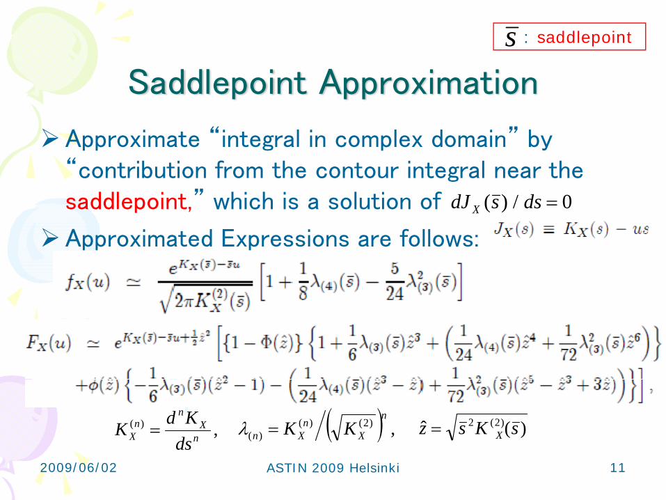
Saddlepoint Approximation

Approximate “integral in complex domain” by “contribution from the contour integral near the saddlepoint,” which is a solution of

Approximated Expressions are follows:

: saddlepoints

( ) ,)2()()(

n

Xn

Xn KK=λ,)(n

Xn

nX ds

KdK = )(ˆ )2(2 sKsz X=

0/)( =dssdJ X


It is easy to calculate above approximation formulas when s.v. Xjs are mutually independent.

However, independence cannot be assumed in risk evaluation modelsBecause the dependences between s.v.s are very important.

So, we will apply the saddlepoint approximation to conditional independent models !

s.v. τj, j=1,...,n are (G, P) - conditionally independent,

when T > 0, 0 ≦ t1,...,tn ≦ T,

Application to Risk Evaluation (1)

⎟⎟⎠

⎞⎜⎜⎝

⎛= ∑

=

n

jjj XaX

1


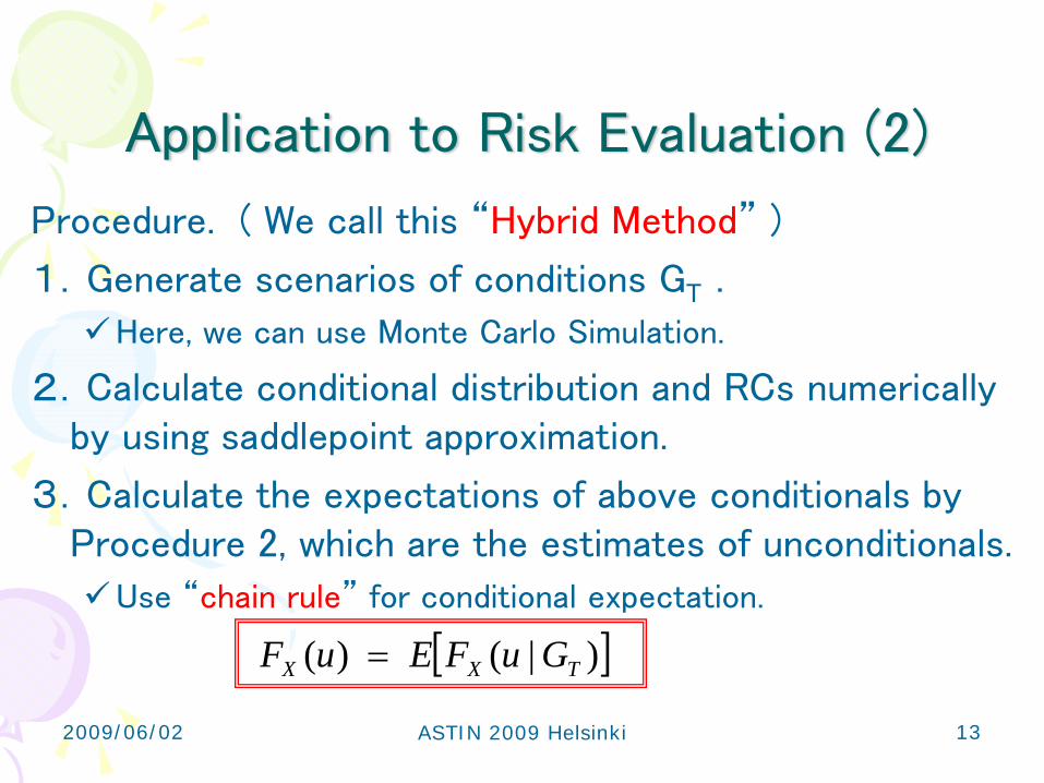
Application to Risk Evaluation (2)

Procedure. ( We call this “Hybrid Method” )

１．Generate scenarios of conditions GT ．

Here, we can use Monte Carlo Simulation.

２．Calculate conditional distribution and RCs numerically by using saddlepoint approximation.

３．Calculate the expectations of above conditionals by Procedure 2, which are the estimates of unconditionals.

Use “chain rule” for conditional expectation.

[ ])|()( TXX GuFEuF =


Old Estimation Method for ES and its RC

Application to ES (and CTE, Conditional Tail Expectation)

Then, written as follows;

where Fh(u) is distribution function whose density is

Saddlepoint approximation can be used to evaluate Fh(u), then, ES (CTE) can be estimated.

RCs for ES (or CTE) can be derived similarly as RCs for VaR.Taking derivative of w.r.t. aj .

))1(()( αα −−= XXX QCTEcES


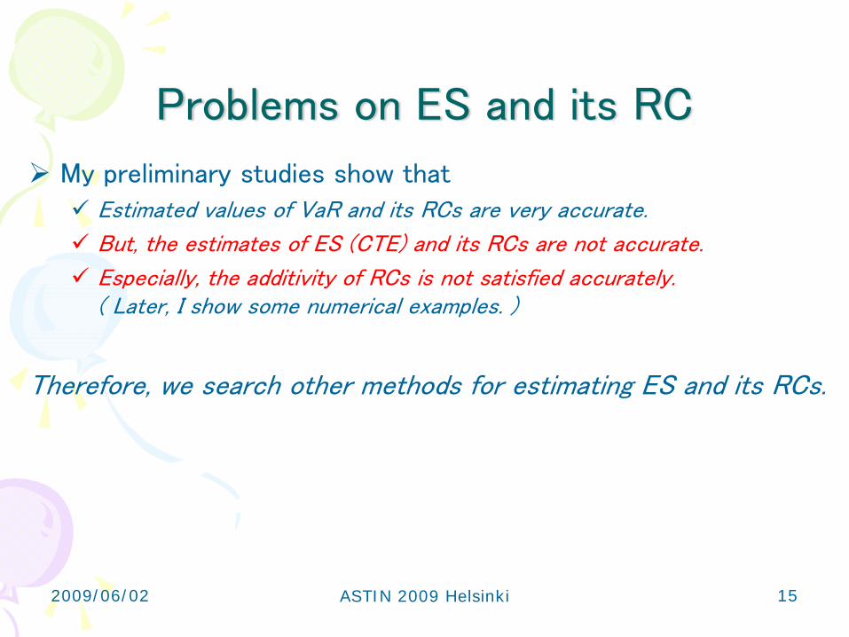
Problems on ES and its RC

My preliminary studies show that Estimated values of VaR and its RCs are very accurate.

But, the estimates of ES (CTE) and its RCs are not accurate.

Especially, the additivity of RCs is not satisfied accurately. ( Later, I show some numerical examples. )

Therefore, we search other methods for estimating ES and its RCs.


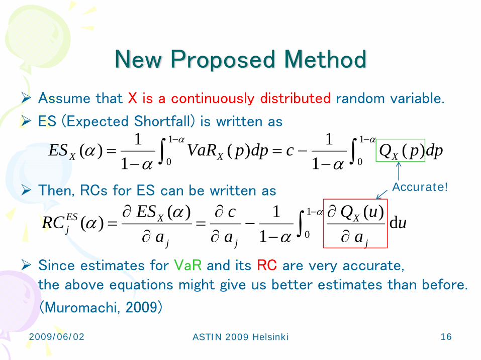
New Proposed Method

∫∫−−

−−=

−=

αα

ααα

1

0

1

0)(

11)(

11)( dppQcdppVaRES XXX

Assume that X is a continuously distributed random variable.

ES (Expected Shortfall) is written as

Then, RCs for ES can be written as

Since estimates for VaR and its RC are very accurate, the above equations might give us better estimates than before.

(Muromachi, 2009)

∫−

∂∂

−−

∂∂

=∂

∂=

α

ααα

1

0d)(

11)()( u

auQ

ac

aESRC

j

X

jj

XESj

Accurate!


3. Numerical Examples(preliminary results)

Setting

Evaluating an interest rate risk and credit risk of a portfolio after 1 year by using a model (Kijima and Muromachi, 2000).

Portfolio : 100 corporate bonds with maturity 5 years.

Credit Rating : Aaa(10), Aa(10), A(10), Baa(10), Ba(30), B(30).

Detailed conditions are omitted here. Please read our article.

Monte Carlo simulation: 500,000 scenarios. use as a reference.

Hybrid Method with importance sampling technique. See Muromachi (2004) in detail.

ES and its RCs are estimated by old and new methods.


Estimated VaR and ES

In next slide, we show the difference.

Con

fiden

ce le

vel

old method

new method


Estimated Difference : ES - VaR

Confidence level

ES －

VaR

“IS-H” differs from “simulation”.“from VaR” is much better.

old method

new method


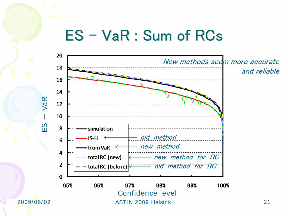
ES – VaR : Sum of RCsES

－Va

R

old methodnew method

new method for RCold method for RC

New methods seem more accurate and reliable.

Confidence level212009/06/02 ASTIN 2009 Helsinki

RC for Percentile and CTE (Baa, 30)Ris

k Con

trib

utio

n

Confidence level

RC for CTE

RC for Percentile


Conclusion

Our method by using saddlepoint approximation gives much more reliable estimates than ordinary Monte Carlo simulation.

Especially, our original method gives very good estimates of (1) VaR and (2) RC for VaR, but not so good of (3) ES and (4) RC for ES.

However, our new proposed method gives good estimates of (3) ES and (4) RC for ES in wide ranges.

This is our first preliminary results. Please wait for more detailed results.


References

Glasserman, P., “Measuring marginal risk contributions in credit portfolio,” Journal of Computational Finance, 9(2), 2005/2006.

Kijima, M. and Y. Muromachi, “Evaluation of credit risk of a portfolio with stochastic interest rate and default processes,” Journal of Risk, 3(1), 2000.

Martin, R., et. al, “VaR: who contributes and how much?” RISK, August, 2001.

Muromachi, Y., presentation in ABR (Applied Business Research Conference), 2009.

Muromachi, Y., “A conditional independence approach for portfolio risk evaluation,” Journal of Risk, 7(1), 2004.


Thank you for your attention.

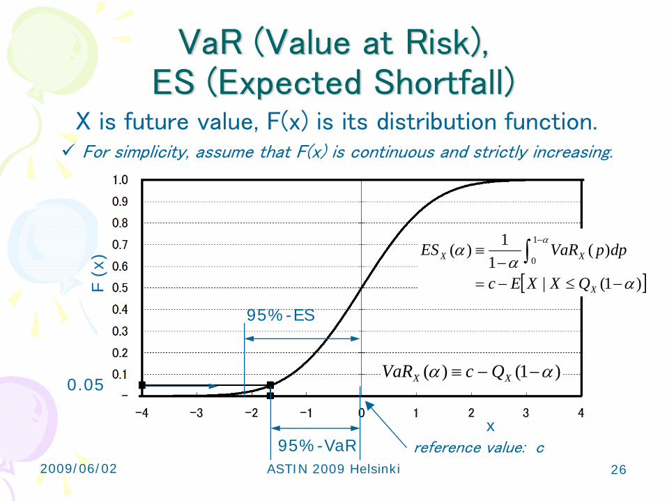
VaR (Value at Risk),ES (Expected Shortfall)

X is future value, F(x) is its distribution function.For simplicity, assume that F(x) is continuous and strictly increasing.

0.05

95%-VaR

95%-ES

reference value: c

F (x

)

x

)1()( αα −−≡ XX QcVaR

[ ])1(|

)(1

1)(1

0

αα

αα

−≤−=−

≡ ∫−

X

XX

QXXEc

dppVaRES


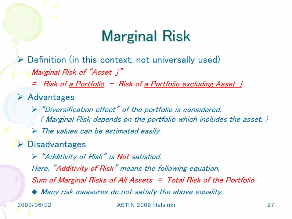
Marginal Risk

Definition (in this context, not universally used)Marginal Risk of “Asset j”

= Risk of a Portfolio – Risk of a Portfolio excluding Asset j

Advantages“Diversification effect” of the portfolio is considered. ( Marginal Risk depends on the portfolio which includes the asset. )

The values can be estimated easily.

Disadvantages“Additivity of Risk” is Not satisfied.

Here, “Additivity of Risk” means the following equation.

Sum of Marginal Risks of All Assets = Total Risk of the Portfolio

Many risk measures do not satisfy the above equality.


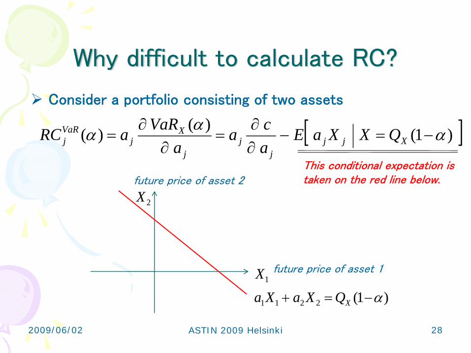
Why difficult to calculate RC?

Consider a portfolio consisting of two assets

[ ])1()()( ααα −=−∂∂

=∂

∂= Xjj

jj

j

Xj

VaRj QXXaE

aca

aVaRaRC

1X

2X

)1(2211 α−=+ XQXaXa

This conditional expectation is taken on the red line below.

future price of asset 1

future price of asset 2


Estimated ES by 3 Methods

“ES (IS-H)” differs from “ES”. “ES (from VaR)” is much better.

old method

new method

Con

fiden

ce le

vel


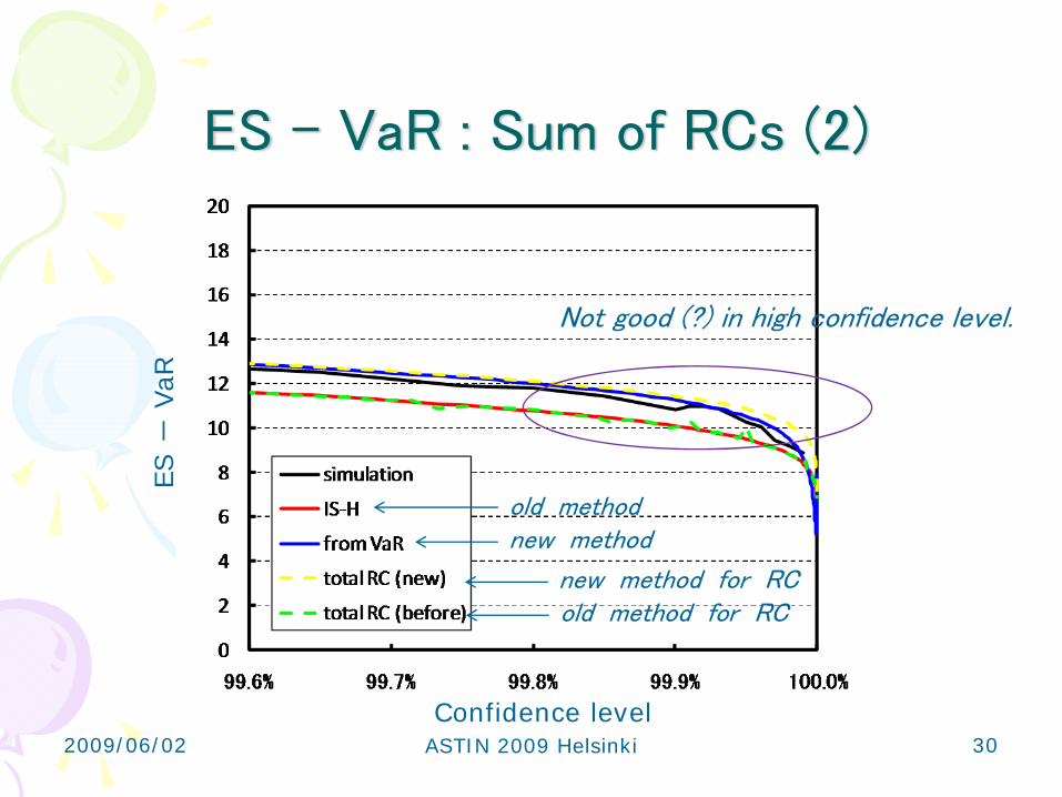
ES – VaR : Sum of RCs (2)ES

－Va

R

old methodnew method

new method for RCold method for RC

Not good (?) in high confidence level.

Confidence level302009/06/02 ASTIN 2009 Helsinki

decomposing total risk of a portfolio into the … total risk of a portfolio into the contributions...

Documents