epri ocean energy

E2I EPRI Specification

Guidelines for Preliminary Estimation of Power Production by Offshore Wave Energy Conversion Devices

Report: E2I EPRI - WP - US - 001 Authors: George Hagerman and Roger Bedard Date: December 22, 2003

E2I/EPRI Guidelines for Preliminary Estimates of Power Production by WEC Devices

Table of Contents

1. Background 2. Wave Energy Resource Specification 3. Power Production Estimating Guideline 4. Requested Performance Documentation 5. References 6. Performance Data Templates for Scatter Diagram Rectangular Sections

Contributing 85% of Total Annual Wave Energy at: a. Maine Reference Station.......................................... NDBC 44005 b. Massachusetts Reference Station............................. NDBC 44008 c. California Reference Station.................................... NDBC 46012 d. Oregon Reference Station........................................ CDIP 0037 e. Washington Reference Station................................. CDIP 0036 f. Hawaii Reference Station ........................................ CDIP 0098

Appendix – Wave Energy Joint Probability Distribution – JPD (included as separate electronic file <E2I EPRI Tp-based JPD Summary.xls>

_________________________________________________________________________ 2


1. Background

Published data on Offshore Wave Energy Conversion (OWEC) devices seldom provide sufficient detail to assess the accuracy of power production claims. The offshore wind energy industry routinely publishes turbine performance data in the form of curves and/or tables depicting generated power as a function of wind speed (see General Electric 3.6 MW turbine at http://www.gepower.com/prod_serv/products/wind_turbines/en/index.htm, or Vestas 2.0 MW turbine at http://www.natwindpower.co.uk/northhoyle/gsv80.pdf for examples), yet wave energy developers rarely provide similar data on generated power as a function of seastate. One goal of the E2I/EPRI Offshore Wave Energy Feasibility Demonstration Project is to determine whether the offshore wave energy industry has reached a level of commercial maturity that can provide customer confidence in advertised claims of power production and the associated cost of energy. This lack of documentation also makes it difficult to compare the likely performance of different OWEC devices in a given wave climate, particularly when different underlying assumptions and simulation or model test methods have been used to generate their power production estimates. Finally, without such documentation, it is impossible to establish a “baseline” performance against which industry improvements can be benchmarked. In order to overcome these hurdles and enable the E2I/EPRI team to select the best OWEC device for each state and estimate the energy production of different devices at various sites with a known degree of confidence, this attachment provides:

• A common resource specification to be used by all developers responding to this Request for Information (RFI)

• A guideline that all developers should use in applying their performance data to this resource specification

• A request for specific documentation of developer-supplied performance data

These three items are covered as separate topics below. This specification then provides blank table templates for the performance data (capture width ratios) that we are requesting.

2. Wave Energy Resource Specification (a) Rationale for Choosing Reference Measurement Stations This specification is based on “reference stations” that the E2I/EPRI team believe best represent the long-term offshore wave climate in each of the six states participating in this study: Maine, Massachusetts, California, Oregon, Washington, and Hawaii. These are not necessarily the sites where a demonstration project or a commercial wave power plant would be built, but instead are sites that are sufficiently far offshore that they represent a state’s most energetic wave climate along a broad section of coast. These stations also were chosen because they have long, relatively continuous wave measurement records (in some cases up to 20 years), comparable to the service life of a wave power plant.

_________________________________________________________________________ 3

http://www.gepower.com/prod_serv/products/wind_turbines/en/index.htm

http://www.natwindpower.co.uk/northhoyle/gsv80.pdf


During the Site Selection task of this study, the E2I/EPRI team will correlate the wave data at each reference station with other, shorter-term data available at other measurement stations and at numerical hindcast grid points across the continental shelf off each state. Two products from this task will be a preliminary wave energy resource map for each state and an environmental design data set for the most promising demonstration site in each state. The environmental design data set will include an annual and twelve monthly joint probability distribution tables of significant wave height and peak wave period at the selected demonstration site, characterization of the 100-year storm event that any project at that site must survive (in terms of wind, wave, and current conditions), and characterization of seafloor bathymetry and geological conditions for mooring system design. The Site Selection task will consider not only the available wave energy resource, but also other key factors such as coastal load growth and the need for power, suitability of onshore grid connection points and transmission capacity, potential environmental conflicts and associated permitting requirements, and proximity to protected harbor areas with suitable fabrication yards and marine equipment for inspection, maintenance, and repair. This will be an iterative process involving our state partners and those wave energy developers that already may be pursuing a project at a particular site in a given state and are willing to collaborate with the E2I/EPRI team to leverage their efforts. From the above description of the Site Selection task it is clear that it would be premature at this point to specify the wave energy resource at a particular demonstration site, since these sites have yet to be selected. Yet the E2I/EPRI team wants to provide developers at the outset with a reasonably accurate characterization of each state’s offshore wave energy resources in terms of characteristic wave height and period distributions, so that developers can submit preliminary information for their devices based on this initial specification as input to our device screening process. The E2I/EPRI team also needs a common resource specification to which developers can apply their performance data, such that the likely energy production of different OWEC devices can be compared in different states. Below is a description of the six reference stations for this specification.. (b) Description of Reference Measurement Stations The two largest inventories of long-term measured wave data in the United States are maintained by the National Data Buoy Center (NDBC) of the National Oceanic and Atmospheric Administration (http://www.ndbc.noaa.gov), and by the Coastal Data Information Program (CDIP) of Scripps Institution of Oceanography (http://cdip.ucsd.edu/). NDBC data buoys are equipped with strapped-down accelerometers for measuring wave conditions derived from buoy heave response. Wave spectra are computed from 20-minute time-series measurements of sea surface elevation changes, and these records are archived at one-hour intervals. CDIP offshore wave measurements are made almost exclusively made by Datawell Waverider® buoys, but offshore oil and gas production platforms also are used when available, to mount submerged pressure gages. Wave spectra are computed from 17-minute time-series measurements of sea surface elevation changes, and these records are archived at six-hour intervals.

_________________________________________________________________________ 4

http://www.ndbc.noaa.gov/

http://cdip.ucsd.edu/


The six reference stations used for this study are listed in Table 1 and mapped in Figures 1 through 3. Annual average wave energy scatter diagrams from these stations have been supplied electronically to all developers receiving this specification as an Excel workbook file named <EPRI Tp-based JPD summary.xls>.

Table 1. E2I/EPRI Offshore Wave Energy Reference Measurement Stations Station Latitude Longitude Depth Measurement State Number Station Name (deg N) (deg W) (m) Period (years)

ME NDBC 44005 Gulf of Maine 43.18 69.18 22 1983 – 2002

MA NDBC 44008 Nantucket Shoals 40.5 69.43 63 1983 – 2002

CA NDBC 46012 Half Moon Bay 37.4 122.7 80 1983 – 2002

OR CDIP 0037 Coquille River 43.11 124.51 64 1985 – 1996

WA CDIP 0036 Grays Harbor 46.86 124.07 38 1987 – 2002

HI CDIP 0098 Makapuu Point 21.32 157.59 91 1982 – 1996

Figure 1. New England Wave Measurement Stations (NDBC stations 44005 and 44008 symbolized by bright green squares)

_________________________________________________________________________ 5


Figure 2. West Coast Wave Measurement Stations (NDBC station 46012 symbolized by bright green square;

CDIP stations 0036 and 0037 symbolized by bright green circles)

Figure 3. Oahu, Hawaii Wave Measurement Stations (CDIP station 0098 symbolized by bright green circle)

(c) Development of Wave Energy Scatter Diagrams

_________________________________________________________________________ 6


To develop the wave energy scatter diagrams for this initial resource specification, seastate parameter records were read to extract the significant wave height (Hs in m), and the peak wave period (Tp in sec), which is the inverse of the frequency at which the wave spectrum has its maximum value for the measured seastate record. Based on these two parameters, the incident wave power (J in kilowatts per meter of wave energy device width, or kW/m) associated with each seastate record was estimated by the following equation:

J = 0.42 x (H s)2 x Tp (Equation 1)

The 0.42 multiplier in the above equation is exact for any seastate that is well represented by a two-parameter Bretschneider spectrum, but it could range from 0.3 to 0.5, depending on the relative amounts of energy in sea and swell components and the exact shape of the wave spectrum. Although such an estimate, based solely on the parameters H s and Tp, is not exact, it was deemed adequate for this initial specification.

For the environmental design data set that will be developed for each state’s selected demonstration site, a more accurate estimate is needed, and for this purpose the E2I/EPRI team will use the original archived spectra to exactly calculate incident wave power from spectral moments (as outlined in Reference 1). Once the seastate parameters were read, and Equation 1 used to estimate the incident wave power for a given measurement record, the record was sorted into the appropriate seastate bin according to the values of Hs and Tp for that record. Once all records were thus sorted, the number of records in each bin was divided by the total number of records in the entire measurement period. This yielded the percentage of time that a given seastate bin occurs, and when multiplied by 8766 hours in an average year (accounting for 29 days in February every fourth year), this gives the number of hours that each seastate occurs. Multiplying the number of hours that each seastate occurs by the incident wave power density (in kW/m) for that bin yields the wave energy contribution (in kWh/m) of that bin. Summing the wave energy contribution across all bins and dividing by the number of hours in a year yields the annual average incident wave power at the reference location. The accompanying Excel file contains just the wave energy scatter diagrams for each reference station. Any developer wanting to see the intermediate calculation sheets for a particular station should contact the E2I/EPRI Project Manager, Roger Bedard, who can provide the full workbook, which contains the raw scatter diagram, the joint probability distribution table, the number of hours that each seastate occurs during an average year, the wave energy scatter diagram, and the estimated incident wave power in each seastate, as calculated by Equation 1, assuming a Bretschneider two-parameter wave spectrum. 3. Power Production Estimating Guideline A rectangular section from the wave energy scatter diagram for the Makapuu Point reference station in Hawaii is shown below. Note that seastates in the bin of H s = 2 m and Tp = 9 sec contribute an average of 8,313 kWh of incident wave energy per meter’s width of any OWEC device installed at that location.

_________________________________________________________________________ 7


Hawaii Annual Wave Energy Scatter Diagram (kWh per meter per year)

Tp (sec) Hs (m) 6 7 8 9 10 11 12 13 14 3 17 533 1,522 3,389 1,696 1,407 1,794 2,167 1,127

2.5 629 2,285 5,118 6,423 2,346 2,404 3,246 3,413 1,7892 3,013 4,087 7,926 8,313 2,938 3,886 5,443 5,232 2,433

1.5 2,229 2,415 4,717 4,456 2,034 2,941 3,734 3,798 2,057 Even without obtaining the full workbook for this reference station, one can estimate the incident power in this seastate from Equation 1 on the previous page as 15.12 kW/m, using the midpoints of the bin categories for H s and Tp. From this result it is a simple matter to back-calculate that this particular seastate bin occurs 550 hours per year, or about 6.3% of the time. Also note that 85% of the total annual offshore wave energy resource off Hawaii is contained within these 36 seastate bins. The Excel file accompanying this specification has highlighted for each state the rectangular sections that contain roughly 85% of the annual wave energy resource, and these are the basis for the table templates. Thus our initial screening will be based on comparing device wave energy absorption within the “85% rectangular sections” given at the end of this specification, and interested wave energy developers should enter their performance data in the table template(s) for the state(s) of their choice. Each cell in a table should contain a developer’s best estimates of the “capture width ratio” of the devices when operating in a random seaway having the same Hs and Tp as the midpoints of the seastate bin associated with that cell. The capture width ratio of a device for a particular seastate should be calculated as the absorbed power (before losses in conversion to electric power) resulting from a particular seastate numerical simulation (or random wave model test) divided by the product of the incident wave power for that simulation (or test) and the width of the simulated device (or model). Thus if capture width ratio is symbolized as CWR, then the equation is:

CWR = Pabs / (J x Dy) (Equation 2)

where CWR is the capture width ratio (dimensionless – no units), Pabs is the absorbed power in simulated or modelled seastate (e.g. in kW/), J is the incident power in simulated or modelled seastate (e.g. in kW/m), and Dy is the cross-wave dimension of the simulated device or test model (e.g. in m), which would be the diameter of a cylindrical buoy or beam of a rectangular raft.

For example, consider the numerical simulation results published by the wave energy research group at the Norwegian Institute of Technology (NTH), University of Trondheim for a slack-moored, heaving-cylinder device with phase control (Reference 2, which can be downloaded at http://www.phys.ntnu.no/instdef/prosjekter/bolgeenergi/simwec.pdf). The wave energy absorber is a cylindrical spar buoy, 3.3 m in diameter, having a molded depth of 5.1 m. A reaction plate, 8 m in diameter, is suspended from the buoy, in line with a double-acting hydraulic cylinder. The reaction plate is submerged 10 m below the sea

_________________________________________________________________________ 8

http://www.phys.ntnu.no/instdef/prosjekter/bolgeenergi/simwec.pdf


surface, and relative motion between the buoy and plate strokes the cylinder, absorbing wave energy by converting work done on the buoy and plate by waves into fluid work. This is a useful example because it illustrates how to handle the mismatch that occurs when device performance data are based on simulated or test seastates characterized by mean zero-crossing period (Tz) rather than the peak period characterization (Tp) that is used in this specification. It also illustrates how to extrapolate a limited set of simulation or test results to Hs - Tp seastate bins that have not been simulated or tested. On page 17 of the above NTH paper, Table 9 lists the following results for numerical simulations of Pierson-Moskowitz (P-M) spectra, based on a 100-second steady-state simulation. The P-M spectrum is a special case of the Bretschneider spectrum, in which

Tp = Tz / 0.710 (Equation 3)

This equation should be used to convert Tz -based simulation or test results from P-M spectra to Tp for calculating the incident wave power during the simulations or test runs.

The P-M spectrum simulation results from Reference 2 are tabulated below. The top row indicates the mean-zero crossing period (Tz), and the second row indicates the associated peak period (Tp) calculated by Equation 3. The third row indicates the significant wave height (Hs), the fourth row indicates the absorbed power result (Pabs), and the fifth row indicates the incident wave power (J) calculated by Equation 1. Based on the buoy’s diameter of 3.3 m, the last row of the table indicates the capture width ratio (C) in each seastate, as calculated by Equation 2.

NTH Simulation Results for Slack-Moored Heaving Buoy in P-M Spectra Tz (sec) 3.8 4.3 4.9 5.3 5.9 6.4 6.9 7.4 7.9 Tp (sec) 5.4 6.1 6.9 7.5 8.3 9.0 9.7 10.4 11.1 Hs (m) 0.9 1.3 1.6 2.0 2.4 2.9 3.4 4.0 4.6

Pabs (kW) 2.5 3.8 5.3 6.6 7.7 9.2 11.2 12.7 14.9 J (kW/m) 1.8 4.3 7.4 12.5 20.1 31.8 47.2 70.0 98.9

C 0.42 0.27 0.22 0.16 0.12 .088 .072 .055 .046 The next step is to map these capture width ratio results into the appropriate Hs - Tp bins of the “85% rectangular section” of the wave energy scatter diagram, which is done for the Hawaii station in the table below.

Capture Width Ratios for Hawaii Wave Energy Scatter Diagram Tp (sec) Hs

(m) 6 7 8 9 10 11 12 13 14 3 .134 .108 .097 .088 .077 .070 .064 .059 .055

2.5 .161 .130 .116 .105 .093 .084 .077 .071 .065 2 .201 .162 .145 .131 .116 .105 .096 .088 .082

1.5 .268 .216 .193 .175 .154 .140 .128 .118 .109

_________________________________________________________________________ 9


Note that only five of the NTH results (shaded in black and white print and yellow-shaded bins, red font in color print) map into the Hs - Tp distribution where 85% of the incident wave energy occurs in Hawaii. In a case such as this, the developer must either conduct new simulations targeted at the remaining 31 bins in the above table, which is the preferred approach, or the developer can fit a capture width ratio function to existing results that fall outside the “85% rectangular section,” yielding CWR as a function of Hs and Tp and applying this function to the empty bins. For example, in Reference 2, Pabs is shown to be linearly proportional to Hs. Since J is proportional to (Hs)2, it follows that CWR can be extrapolated according to the ratio 1/( Hs). This factor has been used to fill in the missing CWR values in the first four columns of the above table (italicized blue font). CWR as a 2nd-order polynomial function of Tp for a given Hs can then be fitted to the first four elements in each row, enabling extrapolation of CWR values into the last five columns (bold italicized green font). Multiplying the CWR in each bin by the incident wave energy (kWh/m/yr) in that same bin yields the annual amount of energy absorbed from seastates in that bin per meter of buoy diameter. Summing these products across all 36 bins shows that this device would absorb 12.3% of the wave energy in the entire section. Energy production estimates derived from extrapolation clearly will be much more uncertain than targeted simulations or model tests. All other things being equal, the E2I/EPRI team will more favorably rank a developer that has a numerical simulation model that they can use to conduct simulations specifically targeted at the full range of Hs and Tp bins in the table templates of the appendices than a developer who can only extrapolate results from previous simulations or tests. 4. Requested Performance Documentation For each state in which developers want their devices to be considered, they should enter their performance data into a table with the same number of columns and rows as the highlighted “85% rectangular section” in the wave energy scatter diagram for the state(s) of their choice. Each cell in this table should contain a developer’s best estimates of the capture width ratio (C) of the devices when operating in a random seaway having the same Hs and Tp as the midpoints of the seastate bin associated with that cell. Guidance for how this should be done has been provided on pages 6 through 8 of this specification. Developers also should document how they obtained the absorbed power results (Pabs) used to calculate capture width, as well as providing the cross-wave dimension (Dy) of their full-scale device. The documentation supplied depends on whether the absorbed power results are from numerical model simulations or physical wave tank testing of scale models. (a) For numerical simulation results, the following information is required:

i. Time domain or frequency domain?

ii. Spectrum formula used (P-M, Bretschneider, JONSWAP, etc.)

iii. Duration of simulations (steady-state portion from which results derived)

_________________________________________________________________________ 10


iv. At what model or prototype scale has numerical simulation been physically validated?

v. Validation results: How well does numerical simulation predict measured physical model or prototype output?

(b) For physical model test results, the following information is required:

i. Dimensions of model or prototype

ii. Dimensions (length, width, depth) of model test tank (or water depth and distance from shore for prototypes)

iii. Spectrum formula used (P-M, Bretschneider, JONSWAP, etc.)

iv. Duration of measurements (steady-state portion from which results derived)

_________________________________________________________________________ 11


5. References (1) Therese Pontes: “Mathematical Description of Waves and Wave Energy.” INETI Department of Renewable Energies. Lisbon, Portugal. December 2002. (2) Håvard Eidsmoen: “Simulation of a Slack-Moored Heaving-Buoy Wave-Energy Converter with Phase Control.” Division of Physics, Norwegian University of Science and Technology. Trondheim, Norway. May 1996.

_________________________________________________________________________ 12


6. Performance Data Templates for Scatter Diagram Rectangular Sections Contributing 85% of Total Annual Wave Energy

(a) ME Reference Station: NDBC 44005 – Gulf of Maine

Capture Width Ratios for Maine Wave Energy Scatter Diagram Tp (sec) Hs

(m) 6 7 8 9 10 11 12 5.5 5

4.5 4

3.5 3

2.5 2

1.5 1

(b) MA Reference Station: NDBC 44008 – Nantucket Shoals

Capture Width Ratios for Massachusetts Wave Energy Scatter Diagram Tp (sec) Hs

(m) 6 7 8 9 10 11 12 5.5 5

4.5 4

3.5 3

2.5 2

1.5 1

_________________________________________________________________________ 13


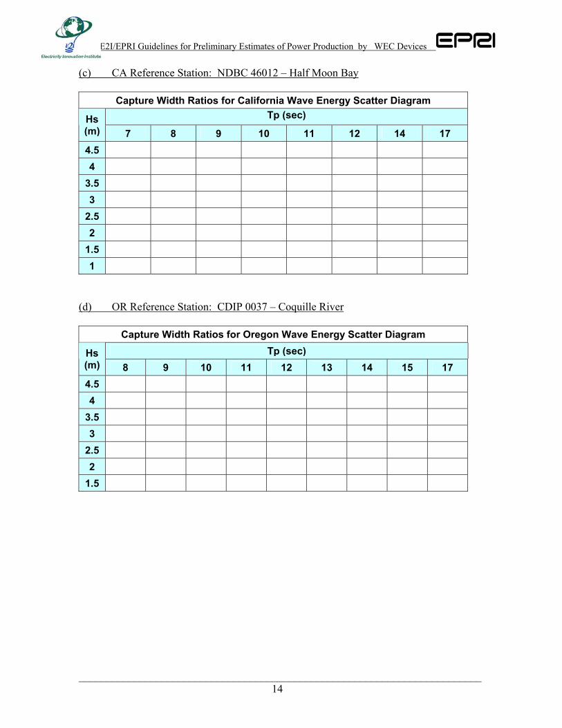
(c) CA Reference Station: NDBC 46012 – Half Moon Bay

Capture Width Ratios for California Wave Energy Scatter Diagram Tp (sec) Hs

(m) 7 8 9 10 11 12 14 17 4.5 4

3.5 3

2.5 2

1.5 1

(d) OR Reference Station: CDIP 0037 – Coquille River

Capture Width Ratios for Oregon Wave Energy Scatter Diagram Tp (sec) Hs

(m) 8 9 10 11 12 13 14 15 17 4.5 4

3.5 3

2.5 2

1.5

_________________________________________________________________________ 14


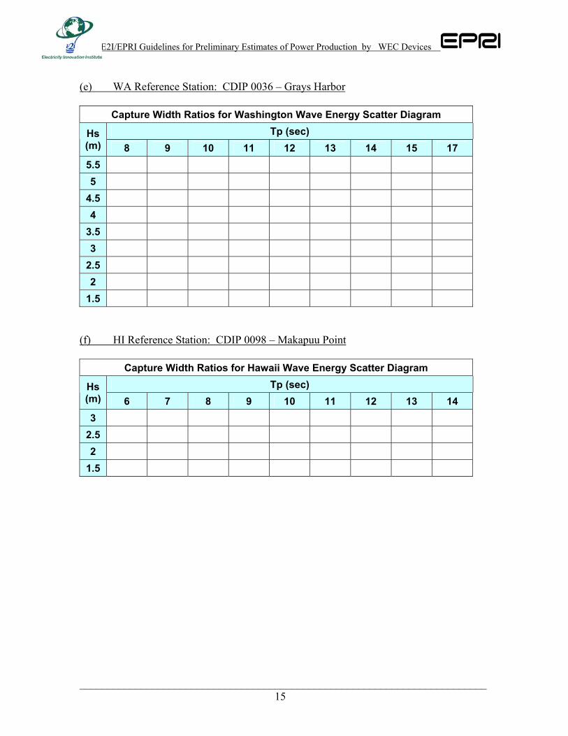
(e) WA Reference Station: CDIP 0036 – Grays Harbor

Capture Width Ratios for Washington Wave Energy Scatter Diagram Tp (sec) Hs

(m) 8 9 10 11 12 13 14 15 17 5.5 5

4.5 4

3.5 3

2.5 2

1.5 (f) HI Reference Station: CDIP 0098 – Makapuu Point

Capture Width Ratios for Hawaii Wave Energy Scatter Diagram Tp (sec) Hs

(m) 6 7 8 9 10 11 12 13 14 3

2.5 2

1.5

_________________________________________________________________________ 15


_________________________________________________________________________ 16

Appendix – Wave Energy Scatter Diagram Excel Workbook <E2I EPRI Tp-based JPD Summary.xls>

1) Maine Reference Station ................................................. NDBC 44005 2) Massachusetts Reference Station .................................... NDBC 44008 3) California Reference Station ........................................... NDBC 46012 4) Oregon Reference Station ............................................... CDIP 0037 5) Washington Reference Station ........................................ CDIP 0036 6) Hawaii Reference Station................................................ CDIP 0098

epri ocean energy

Documents