eoeoeeeindhe - apps.dtic.mil
TRANSCRIPT
D-R143 440 BOUNDRRY-LRYER DEVELOPMENT ON SHIP HULLS(U) DCW i/iI INDUSTRIES SHERMAN OAKS CA D C WILCCX JAN 83I DCN-R-2b-GJ N00014-8i-C-0235
UNCLASSIFIED F/G 20/4 NL
EOEOEEEINDhE

11111L 25 1111 14 11111 1.6Iiii- 111ll- IIIII-
MICROCOPY RESOLUTION TEST CHARTNATIONAL BUREAU OF STANDARDS- 1963-A
i
°, W.Q/
ITI
N<.-
S JUL 2 51984
,i,. 0
* 4367 TROOST AVENUE, STUDIO CITY, CALIFORNIA 91604
• .. -;
DCWMO STATEMETRIE*.--. . . . . . . . . . . . . . . . .
;A . J . ... ! :~.S~ ULA 2 5 98
+ Aw ' App ov d tot p blic ele as%D istition Unlimitod
mlll~l!++ +, q4 10, 7 24 ID77
w7. .1 ._
D.,
BOUNDARY-LAYER DEVELOPMENT
ON SHIP HULLS
by
David C. Wilcox
,i.
FINAL SCIENTIFIC REPORT
January 1983
Prepared Under Contract N00014-81-C-0235
for the
GENERAL HYDRODYNAMICS RESEARCH PROGRAM
OF THE NAVAL SHIP SYSTEMS COMMAND
NAVAL SHIP RESEARCH AND DEVELOPMENT CENTER
Acepssion Fr,'"? GPA&I
V - l
lDCWIndustries Inc.4367 Troost Avenue
Studio City, California 91604 D213/769-7571 or 213/790-3844
APProvod for publir (3l00SA;
: -'I ' ,; , . e . -> ' - *f -" .-"--. . " "-" ""."."- -"-""- "': . " "" """""" "' ,n .- ""

|_.,,, ,., . . . . . _ • .. . .. . -. . . . . - . . .
. UNCLASSIETDSECURITY CLASSIFICATION O
r THIS PAGE (Wen Doe Entered)
REPORT DOCUMENTATION PAGE | ,I1 1.1 T ,
1 O NUM ER 12 GOVT ACCESSION NO ' Fit 'PA N A ft ** Z
14. TITLE (and SubtitlO) S IvP- OF REP9RQ A 4 I _ -- ,. ;
BOUNDARY-LAYER DEVELOPMENT ON SHIP HULLS F URTP.... . i FE 19 31 :. .6 PERFORMING OVG REPORT
DCW-R-26-ol,7. AuTHOR(e) I CONTRACT OR GRANT NUMBER,
DAVID C. WILCOX N
9 PERFORMING ORGANIZATION NAME AND ADDRESS 10 PROGRAM EEMENT PR,'E . TA%,
DCW INDUSTRIES, INC. ARE6WORK ,,' BQ.
4367 Troost AvenueStudio City, CA 91604
11. CONTROLLING OFFICE NAME AND ADDRESS 12 REPORT DATE
DTNSRDC JANUARY 1983Bethesda, MD 13 NUMBER OF PAGES
14 MONITORING AGENCY NAME A AODRESS(I diflerent lrin Controlling Office) 15 SECURITY CLASS (of thi rep<r'
U N CLASS: FI ED
ISe DECLASSIFICATION DOWNZ RAD!; 3SCHEDULE
16. DISTRIBUTION STATEMENT (of thl Report)
Approved for Public Release, Disributicn Unlimited.
17. DISTRIBUTION S'ATEMENT (of the abstract entered in Block 20, it different fro Report)
I. SUPPLEMENTARY NOTES
19 KEY WORDS (Continue on reveree side it neceeery and Identify by block nuiniber)
SHIP HYDRODYNAMICS, THREE-DIMENSIONAL BOUNDARY LAYLU,
THICK BOUNDARY LAYERS
20 AOSTRACT (Continue an reerse side If neceeary end dentlif by block number)
A three-dimensional boundary-layer computer program is de'i ,which is suitable for application to arbitrary shiT hull..
program embodies the Wilcox-Rubesin two-equaticn model of t :,lence. The numerical algorithm, based on the LIottne' vari*. :.-grid method and the Krause explicit marching tec :" 1tested for two ship hulls and found to le accurate a!J stu:for relatively large reverse crossflow. The program air'.:
Ak FORM 17
FAN ,, 1473 EDITION OF I NOV , It O@SOLETE
,SECURITY CLASSIFICATION OF THiS PACE *on Do e .. d.
UNCLASSIFIED5ECURITY CLASSIICATION Of T0IS PAGE(When Die Eftered)
rapid stretching of the grid normal to the surface ax. s.ubecome grid independent for mesh-point number in excess of a'ut
Co fp'risons between computed and measured momentum thicknezs forthe two ship-hull computations indicate that, on the one hand, theWilcox-Rubesin model improves predictive accuracy over that foundat the 1980 SSPA-ITTC Workshop on Ship Boundary Layers. C: . theother hand, discrepancies between computation and measurem.r;' r -mains large enough to warrent further research. Because t .e --putations use conventional thin-shear-layer approximaticrns a-.4discrepancies are largest near the stern, it arpears likely t>aoimproved accuracy can only be obtained by accounting for te fa2tthat the boundary layer becomes "tnick"
To test the model for thick boundary layers, three submerged axl-symmetric bodies are analyzed, viz, a thin cylinder aligned ax-a*with the freestream and two bodies with adverse pressure gradient.Comparisons between computed and measured flow properties for thethin cylinder show the model to be quite accurate in the atsence cf
-' pressure gradient. Using first the measured surface pressure dis-tribution and then the measured boundary-layer-edge pressure dis-tribution, experimental data are found to lie between the tw.' c=-putational results for both bodies. This result indicates that t:
accounting for the normal pressure gradient, model predicticns f-2rthick boundary layers should be very close to measurements. Anintegral method is devised and tested for computing the normalpressure gradient. Differences between computed and measured pres-sure distributions are well within experimental data scatter.
UNCLASC V-I __,
-i iLCUMITV CLASOMPCAION OF *P&GIW*.a. 1f

:1CONTENTS
SECTION PAGE 2ABSTRACT ............................................. ii
CONTENTS ............................................. iv
I INTRODUCTION .......................................... 1
2 EQUATIONS OF MOTION ................................... 3
2.1 The Turbulence Model .............................. 3
2.2 Boundary Conditions ............................... 4
3 NUMERICAL CONSIDERATIONS .............................. 6
3.1 The Numerical Procedure ........................... 6
3.2 Preliminary Test of the Revised Program ........... 9
3.3 Numerical Accuracy Study ......................... 14
4 SHIP-HULL APPLICATIONS ............................... 194.1 SSPA Model 720 ................................... 19
4.1.1 Effect of Girthwise Integration Direction..19
4.1.2 Effect of Mesh Refinement .................. 20
4.1.3 Comparison of Computed and MeasuredMomentum Thickness ......................... 21
4.2 HSVA Tanker ...................................... 23
5 ANALYSIS OF THE THICK BOUNDARY LAYER ................. 26
5.1 Perturbation Analysis ............................ 265.1.1 Sublayer Scaling ........................... 26
5.1.2 Wall-Layer Scaling ......................... 28
5.2 Flow Past a Wire ................................. 30
5.3 Bodies with Adverse Pressure Gradient ............ 35
5.3.1 Integral Properties ........................ 355.3.2 Velocity and Reynolds-Stress Profiles ...... 38
5.3.3 Turbulence Properties ...................... 405.3.4 Streamline-Curvature Effects ............... 40
5."4 Pressure Variation in a Thick Boundary Layer ..... 44
6 DISCUSSION...... ............... ........... . .... .......... .50
REFERENCES ......................:.....................52
APPENDIX: PROGRAM LISTINGS ........................... 54
A.1 PROGRAM SHPMSH ............................... 54
A.2 PROGRAM VELOC ................................ 71
A.3 PROGRAM EDDY3 ................................ 84
-iv-

, u • + . + . o,+.+.4 - . r " - r------.'.- -'. -. . -." . -" . .+ ... . .
1. INTRODUCTION
Increasingly there is a need to more accurately predict the viscous
resistance on ship hulls, particularly in light of modern-day fuel
costs. The rapid increase in fuel costs cries out as a mandate
to ship-hull designers to reduce hull resistance, both wave-making
and viscous. Experience has shown that significant advances in
design efficency often require more sophisticated design tools,
and in today's environment, particularly those of the computational
variety.
Airplane and missile designers have had a great deal of success in
developing and utilizing the concept of the "numerical wind tunnel".
As both computational algorithms and accurate engineering sets of
equations describing turbulent fluctuations and stresses have been
developed and improved, so has the ability to replace expensive
wind-tunnel tests by a series of computer runs. In addition to
being relatively inexpensive, such numerical simulations can more
exactly simulate full-scale flow conditions than can wind-tunnel
tests.
In the ship context there is just as pressing a need to replace
expensive tests by numerical simulations. In fact, in light of the
inherent contradiction involved in trying to simultaneously match
Froude and Reynolds numbers, then is an even more pressing need to
utilize the "numerical towing tank" in the design process.
The state of the art of numerical simulations, including viscous
effects, is further advanced in the aerodynamic context then it is
in the hydrodynamic case. Conceptually this is sensible as the
flow past a ship hull involves a free surface and is inherently
three dimensional while, by contrast, much of the flow area over
an airplane wing involves a homogeneous fluid and can be treated
as two dimensional. This two dimensionality has been of especial
value to aerodynamicists as they have been able to Justify focusing
on two-dimensional flows. A great deal of progress in improving
computational efficiency has been made because of the relative
SC Q -1-

simplicity of a two-dimensional computation, progress which would
have been much harder to achieve if the aerodynamicist's primary
application had demanded focusing on three dimensionality. As a
result, computing separated flows can be done today1 at less than2
a percent of the cost seven or eight years ago . And, of course,
these methods are now being implemented in three dimensions.
* Even in three dimensions the aerodynamicist has an easier time of
it than the hydrodynamicist because he needn't deal with a free
surface. Nevertheless, the day of the numerical towing tank draws
nearer and nearer. The purpose of this project has been to help
• in hastening the arrival of the numerical towing tank.
To accomplish this end, we have addressed the viscous portion of
the problem. We have applied a widely-tested two-equation model
• of turbulence (Section 2) to (a) real ship hulls and (b) "thick"
turbulent boundary layers on submerged axisymmetric bodies. The
object of the ship-hull computations has been to test the model's
accuracy in the limit of classical "thin-shear-layer" approximations.
* The latter computations have been done as an attempt to pinpoint
the special characteristics of and to test the model for "thick"
boundary layers.
In performing the analysis we have developed a new three-dimensional
boundary-layer program appropriate to arbitrary ship hulls. A great
deal of the effort in this project focused on devising an accurate
numerical procedure compatible with the turbulence model equations.
Section 3 presents details of the algorithm including a detailed
accuracy study.
In Section 4 we present results of the two ship-hull computations,
including comparison of computed and measured flow properties.
* Section 5 includes details of our thick-boundary-layer study. Re-
sults and conclusions follow in Section 6. The Appendix includes
computer-program listings and an explanation of program input and
output.
-2-
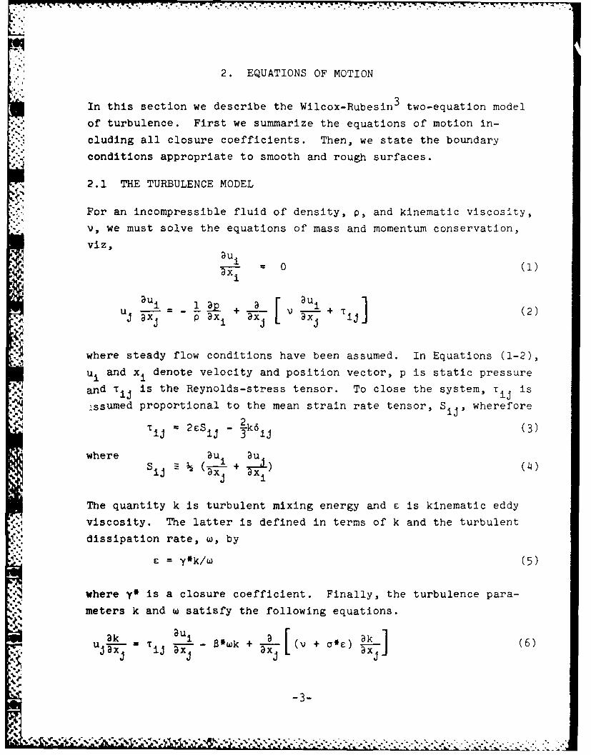
2. EQUATIONS OF MOTION
In this section we describe the Wilcox-Rubesin 3 two-equation model
of turbulence. First we summarize the equations of motion in-
cluding all closure coefficients. Then, we state the boundary
conditions appropriate to smooth and rough surfaces.
N 2.1 THE TURBULENCE MODEL
For an incompressible fluid of density, p, and kinematic viscosity,
v, we must solve the equations of mass and momentum conservation,
viz,au
iau- - o(1)
4..ax 1I
uaui l~ a [ aui 1ujx al [ + (2)axj Pax i ax ax i1j]
where steady flow conditions have been assumed. In Equations (1-2),
ui and xi denote velocity and position vector, p is static pressure
and Tij is the Reynolds-stress tensor. To close the system, Tij is
,ssumed proportional to the mean strain rate tensor, Si , wherefore
i 2ES -2k6 (3)ij 3 IJ
where aui uiij + x (14)
The quantity k is turbulent mixing energy and c is kinematic eddy
viscosity. The latter is defined in terms of k and the turbulent
dissipation rate, w, by
e = y*k/w (5)
where y* is a closure coefficient. Finally, the turbulence para-
meters k and w satisfy the following equations.ak = au I [(v + G'E) aB-Lk
u--wk + (6)-jax i ij ax Tx~L ax iJ
-3-
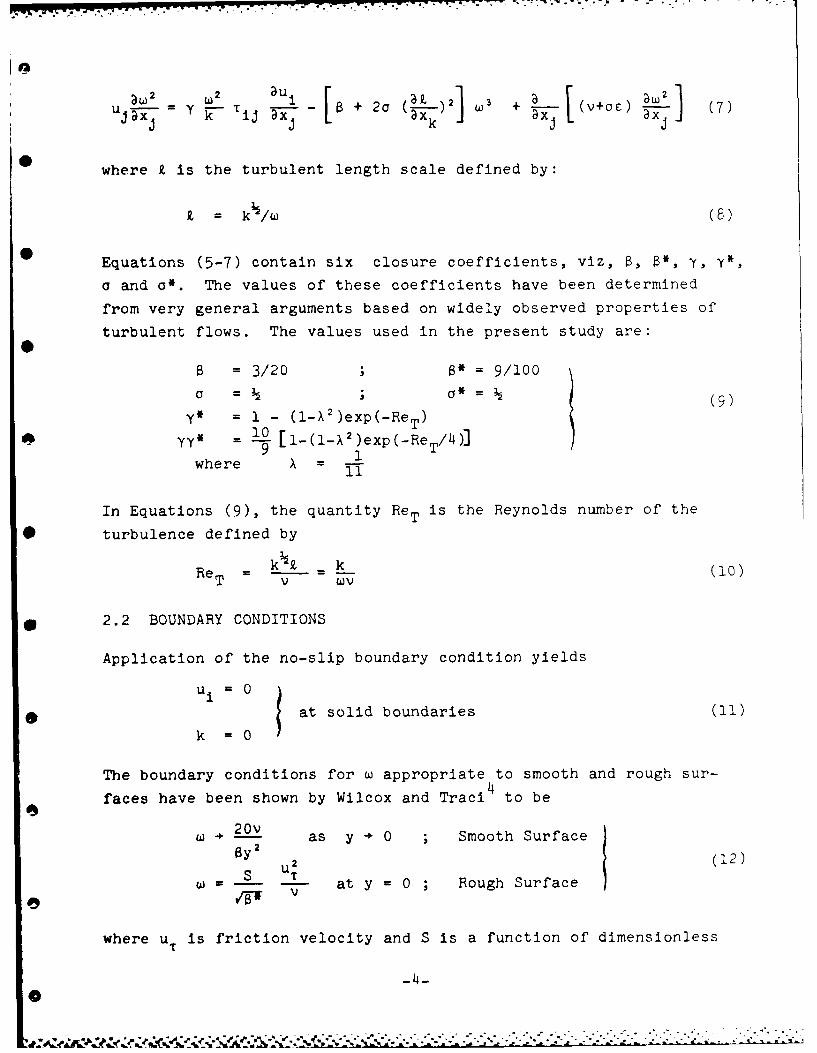
DW2 2 kW-21w w2 -W+ 2cy 2 j 3 X~ + V+ (7)
j k ' jxx kaxx
where k is the turbulent length scale defined by:
= k / (8)
0 Equations (5-7) contain six closure coefficients, viz, Y, , y, y*,
a and a*. The values of these coefficients have been determined
from very general arguments based on widely observed properties of
turbulent flows. The values used in the present study are:
= =3/20 ;* = 9/100
a = k * - (9)y* = 1 - (lX 2 )exp(-ReT)
yy, = LO [l_(lX2)exp(ReT//4)]9 1where X
In Equations (9), the quantity ReT is the Reynolds number of the
* turbulence defined by
ReT - k - k (10)TV WV
* 2.2 BOUNDARY CONDITIONS
Application of the no-slip boundary condition yields
* at solid boundaries (11)
k =0
The boundary conditions for w appropriate to smooth and rough sur-14faces have been shown by Wilcox and Traci to be
20vW 2 as y - 0 ; Smooth Surface
By2 2 (12)
L at y = 0 ; Rough Surface
where uT is friction velocity and S is a function of dimensionless
-4-
' ~~~~- a. . . . . - . . .. . . -. . °.o.
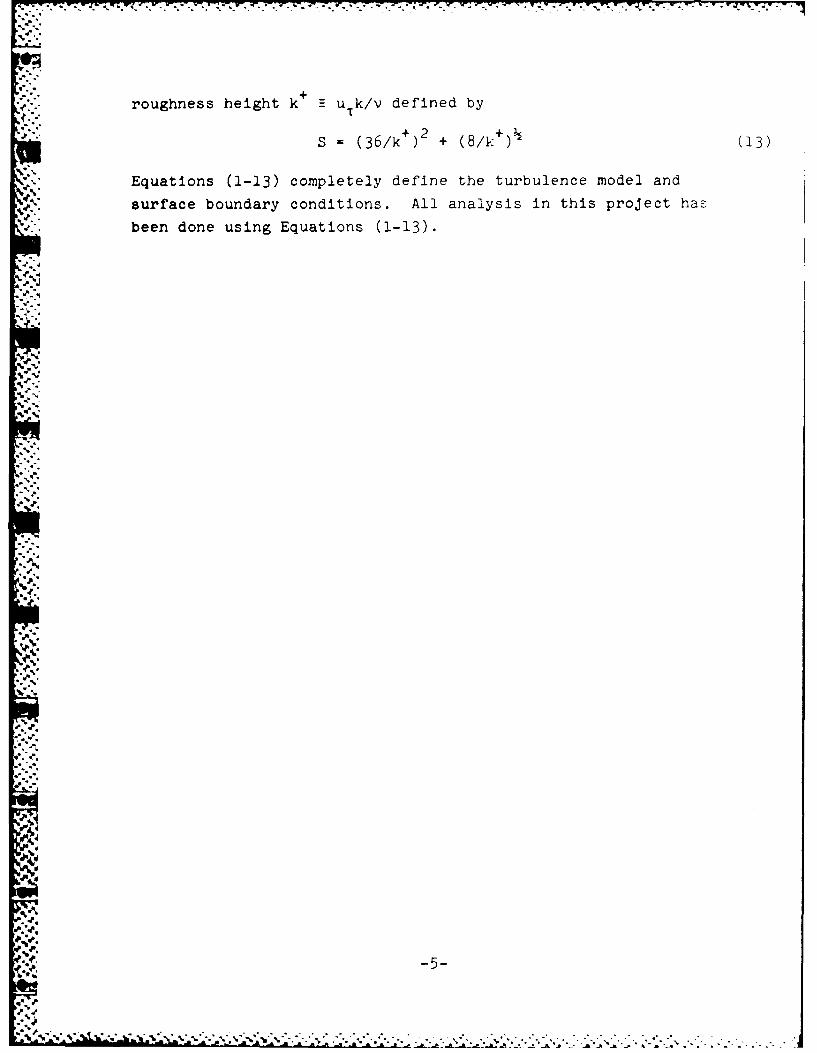
roughness height k+ u k/v defined by
S = (36/k+) 2 + (8/k+) (13)
Equations (1-13) completely define the turbulence model and
surface boundary conditions. All analysis in this project has
been done using Equations (1-13).
|-5-
.'.
*-5-q-
I . !4 : ' ' " :° ," ' " " .' . " ." _ " Z _
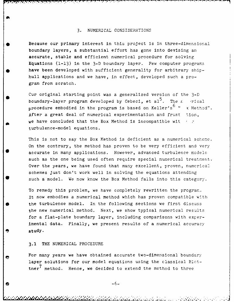
3. NUMERICAL CONSIDERATIONS
* Because our primary interest in this project is in three-dimensional
boundary layers, a substantial effort has gone into devising an
accurate, stable and efficient numerical procedure for solving
Equations (1-13) in the 3-D boundary layer. Few computer programs
• have been developed with sufficient generality for arbitrary ship-
hull applications and we have, in effect, developed such a pro-
gram from scratch.
Cur original starting point was a generalized version of the 3-D
boundary-layer program developed by Cebeci, et al 5 . The r. rical
procedure embodied in the program is based on Keller's 6 " x Method".
After a great deal of numerical experimentation and frust tion,
hwe have concluded that the Box Method is incompatible wit 2
turbulence-model equations.
This is not to say the Box Method is deficient as a numerical scheme.
On the contrary, the method has proven to be very efficient and very
* accurate in many applications. However, advanced turbulence models
such as the one being used often require special numerical treatment.
Over the years, we have found that many excellent, proven, numerical
schemes just don't work well in solving the equations attending
* such a model. We now know the Box Method falls into this category.
To remedy this problem, we have completely rewritten the program.
It now embodies a numerical method which has proven compatible with
* the turbulence model. In the following sections we first discuss
the new numerical method. Next, we show typical numerical results
for a flat-plate boundary layer, including comparisons with exper-
imental data. Finally, we present results of a numerical accuracy
study.
3.1 THE NUMERICAL PROCEDURE
For many years we have obtained accurate two-dimensional boundary
layer solutions for our model equations using the classical Blot-
tner 7 method. Hence, we decided to extend the method to three
.-6-
• ". -, ", -° . . . . . . . .• -. . -. . ... .. . . . . •

dimensions in hopes it wo,' t=Lain its desirable statility a ,u
,- accuracy cbl-teristics. Before embarking on such a major re-
programming effort we made a brief review of Blottner's more re-
.* cent work. We found that, as an improvement to his original pro-
cedure, Blottner8 has devised his "Variable Grid" algorithm. This
• revised method offers far greater accuracy than his original metho,.
particularly for very coarse finite-difference grids. We decided
to use the improved algorithm.
In essence, the "Variable Grid" method uses a conservation for,
treatment for diffusion terms. That is, in the original Elottner
method, diffusion terms must first be expanded according to:
a .. 3 u D2u 3 U (14)
-Y a -, E 2- +
ID'-y
- .'" Then, central difference approximations are used for au/ay, 3c/y,
and a 2 u/ay 2 By contrast, in the improved Blottner method, we write
directly (subscripts denote mesh point number):
E Ju + 6u CJ 6 uay a y(Jyj +Yj-l( - (15)
6u = (u - u )/Ay (I)
and similarly for (6u)j . The quantity Ay. = YJ+l - YJ is the
incremental change in the normal coordinate y. As will be shown
in Subsection 3.3, this straightforward modification permits much
greater stretching of the grid normal to the surface than is pos-
sible with the original Blottner method.
Thus far, we have spoken only of the direction normal to the sur-
face. Because the three-dimensional boundary-layer equations have
a real characteristic which is not necessarily aligned with the
freestream flow direction, any accurate numerical procedure must
be consistent with the attending zone of dependence. The original
Box Method does not treat this problem properly and to avoid
@01 ................................................. t.i:.s s rn,. . J2- 2..
0
future difficulties we decided to accomodate the zone-of-dependence
feature in the revised numerical scheme. In an unpublished study,
Wilcox and James9 devised a family of explicit, unconditionally
stable marching methods which potentially could deal with this
problem. A review of that study showed that most of the family
*were of first-order accuracy. However, one of the most promising
of the family is second-order accurate. Another brief review of
boundary-layer literature showed that this scheme has been used by
many others in three-dimensional boundary-layer applications. The10
scheme is attributed to Krause1 . We have opted to use Krause
scheme in the revised program.
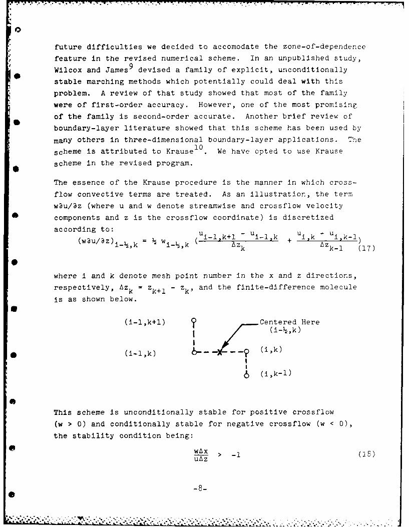
The essence of the Krause procedure is the manner in which cross-
flow convective terms are treated. As an illustration, the tern
wau/Dz (where u and w denote streamwise and crossflow velocity
*components and z is the crossflow coordinate) is discretized
according to: ui k+l - Ui-l~k ui
(wau/3z)i uI 1 k +-uk i~k-1)w i . k i -~ A z k A z( 1 7 )
where i and k denote mesh point number in the x and z directions,respectively, Azk = Zk+ 1 Zk, and the finite-difference molecule
is as shown below.0
(i-l,k+l) Centered Here
(i- ,k)
6 (i(k-1)
This scheme is unconditionally stable for positive crossflow
(w > 0) and conditionally stable for negative crossflow (w < 0),
the stability condition being:
* wAxWAX> -(uAz
-8-
e
'''"-% '"'. -" "". "- '. -'.'-',''.'', <"-< ", "'."........-".."..".-...."•."-."..-',•.....,...

Thus, for equally spaced mesh points (Ax = Az), this scheme is
stable for negative crossflow angles up to 45 degrees from the
streamwise direction.
3.2 PRELIMINARY TEST OF THE REVISED PROGRAM
A key difficulty encountered with the Box Method was the presence
of large round-off errors in the equation for W 2 . Even when wedevised a special procedure to eliminate these errors (caused by
the numerical method's inability to accurately compute the rapid
variation in W 2 as y - 0), nontrivial oscillations in properties
such as skin friction remained. All of these difficulties were
encountered for the simplest boundary-layer of all, the two-
dimensional flat-plate (constant pressure) boundary layer. Hence,
as a preliminary test of our revised 3-D boundary-layer program,
which we will refer to as EDDY3, we focus on the flat-plate boundary
A layer. We have done two somputations, the first for a turbulent
case and the second for a transitional case.
The first computation was initiated from approximate profiles at
a plate-length Reynolds number, Rex, of one million. Using 40
equally spaced streamwise steps, the computation proceeds to a
plate-length Reynolds number of five million. This means the ratio
of streamwise stepsize to boundary-layer thickness ranges from 1.3
to 6.8. Such large steps are comparable to those used in mixing-
length computations. Only 61 mesh points were used normal to the
surface with the grid-point incremental spacing increasing in a
geometric progression with a progression ratio of r = 1.11.
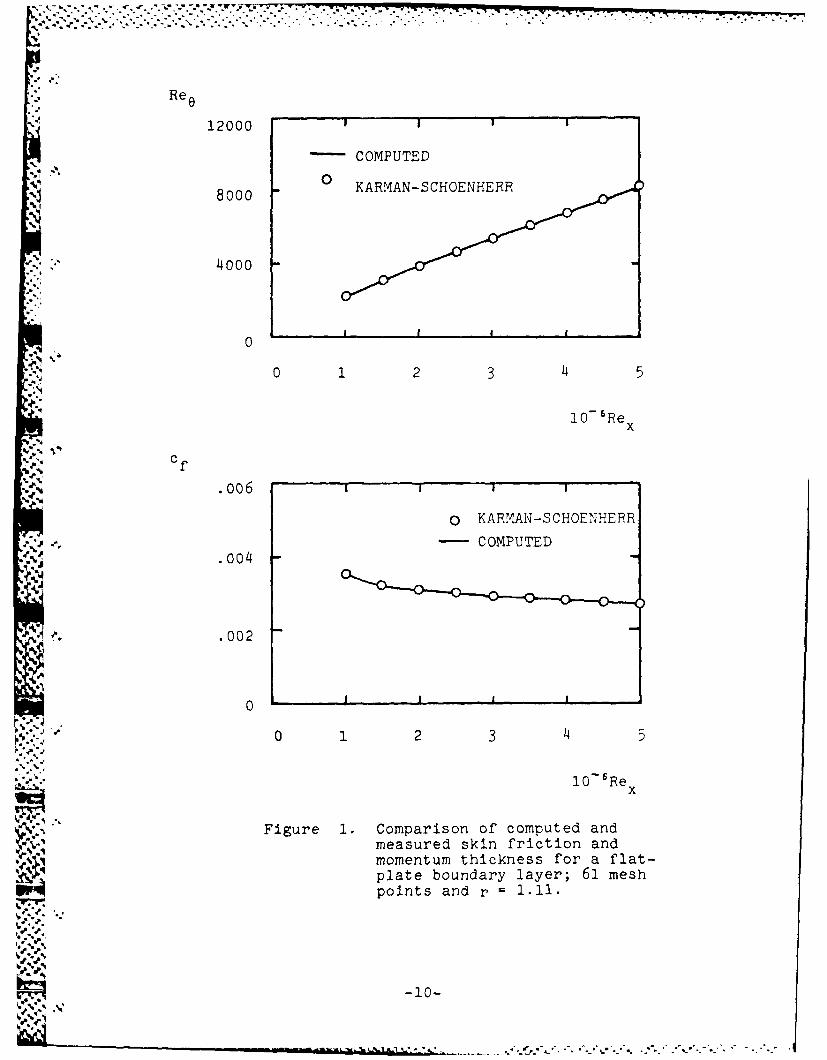
Figure 1 compares computed skin friction, cf, and momentum thick-
neSS Reynolds number, Re., with the Karman-Schoenherr correlation.
As shown, both cf and Re0 virtually duplicate the correlation.
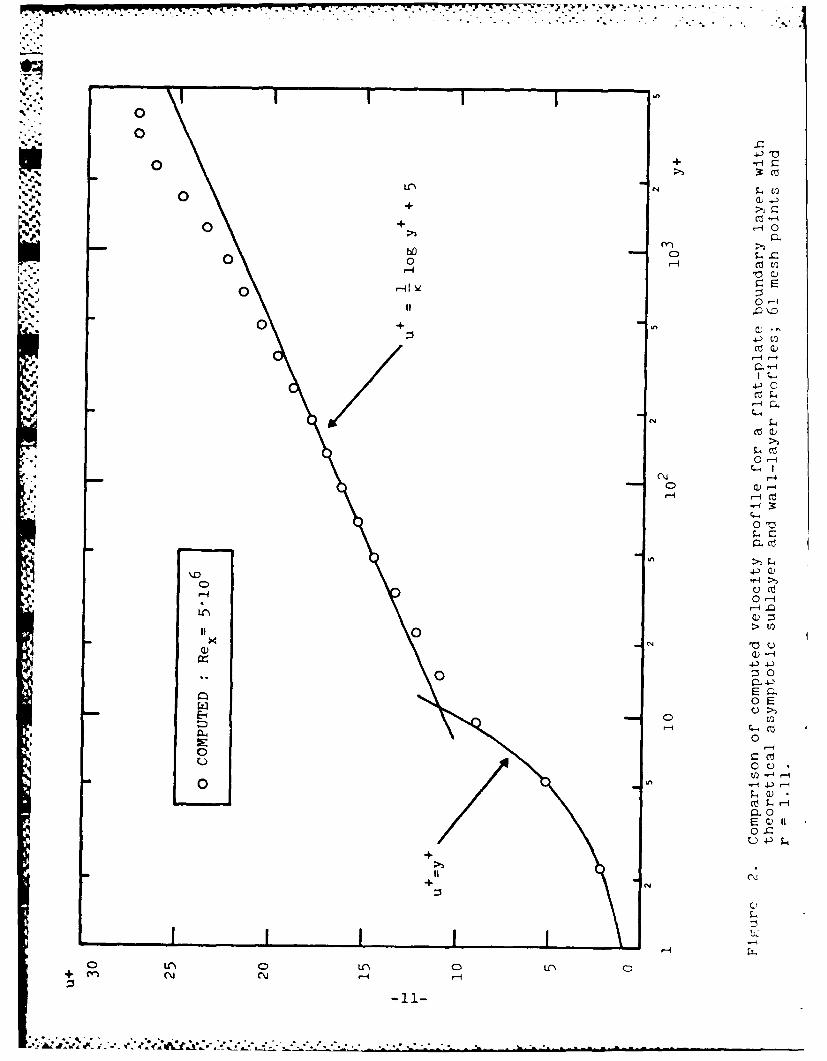
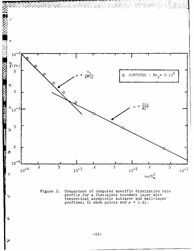
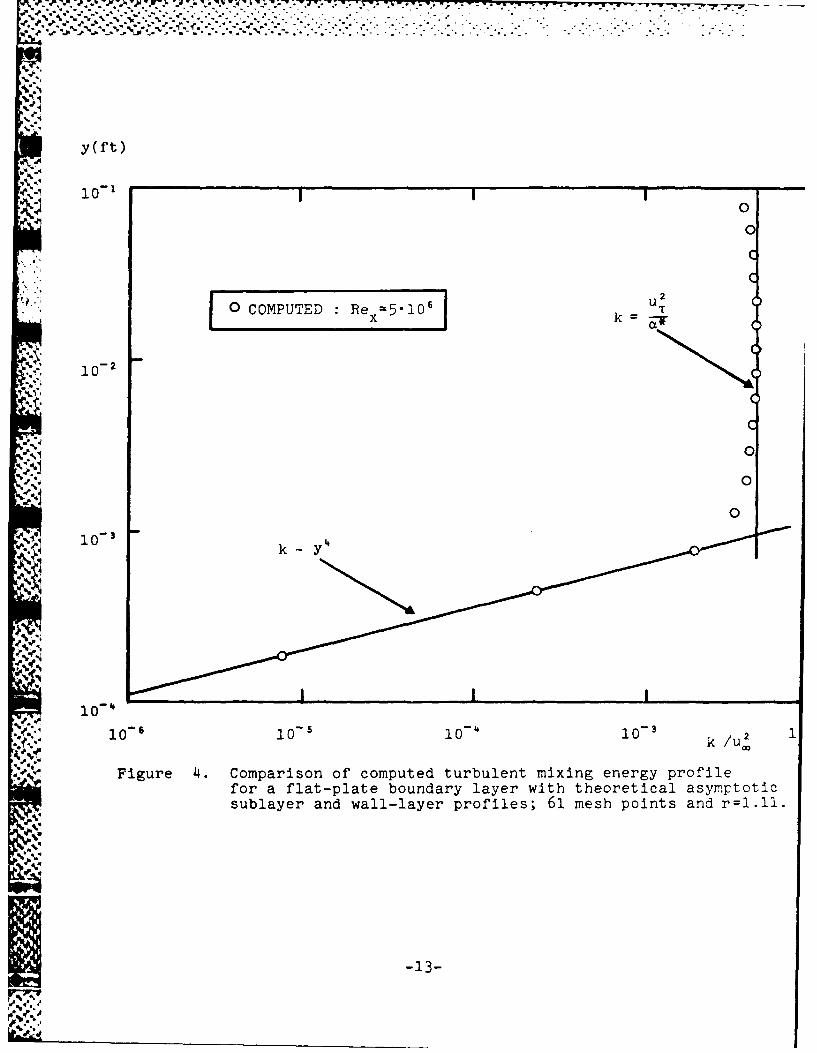
Figures 2 through 4 compare computed velocity, turbulent dissipa-
tion rate and turbulent mixing energy profiles with corresponding
exact theoretical asymptotic sublayer and wall-layer (log region)
profiles. In all cases, the numerical predictions clearly fall
-9-
• Z.Ree
12000 i
- COMPUTED
0 KARMAN-SCHOENHERR8000
*'. 4000
0
0 1 2 3 4 5
10-6 Rem~l x
C
.006 1 1
0 KARMAN-SCHOE'NHERR
f- COMPUTED
.004
.002
' '° 00 2 3
7>,- 00 Re5'.-,
Figure 1. Comparison of computed andmeasured skin friction andmomentum thickness for a flat-plate boundary layer; 61 meshpoints and r = 1.11.
I... *1
-10-
U.4-
0 +
bo C
00
II 0 1
4-) .
C- T4-0
-- 4
C41
4-3
0 E
CL4 0C
0-
00
-A
C -j
F -. .. . . . • P."c
10
'S.,
. y(ft)
= - COMPUTED Rex = 5.106
2 0
S20v
~ o-3 -10-3
y
5
2
l 2 5 2 5o
10 - 4 25 10-3 2510 - 2 2i 0 - I
"I vW/U 2
Figure 3. Comparison of computed specific dissipation rate,j profile for a flat-plate boundary layer with
theoretical asymptotic sublayer and wall-layerprofiles; 61 mesh points and r -- 1.11.
-12-
~y(ft).4
10-1II0
0
t -
(COMPUTED Rex=5-10 k u
O-2
0
0
0io 3
i0-4 -10 /
'," 0" O-S 0- 0- k /uC0
", Figure 4. Comparison of computed turbulent mixing energy profilefor a flat-plate boundary layer with theoretical asymptoticsublayer and wall-layer profiles; 61 mesh points and r=l.!l.
* -13-
.N.
*4 *. .
very close to the asymptotic profiles, thus verifying the accuracy
of the revised numerical procedure in the absence of crossflow.
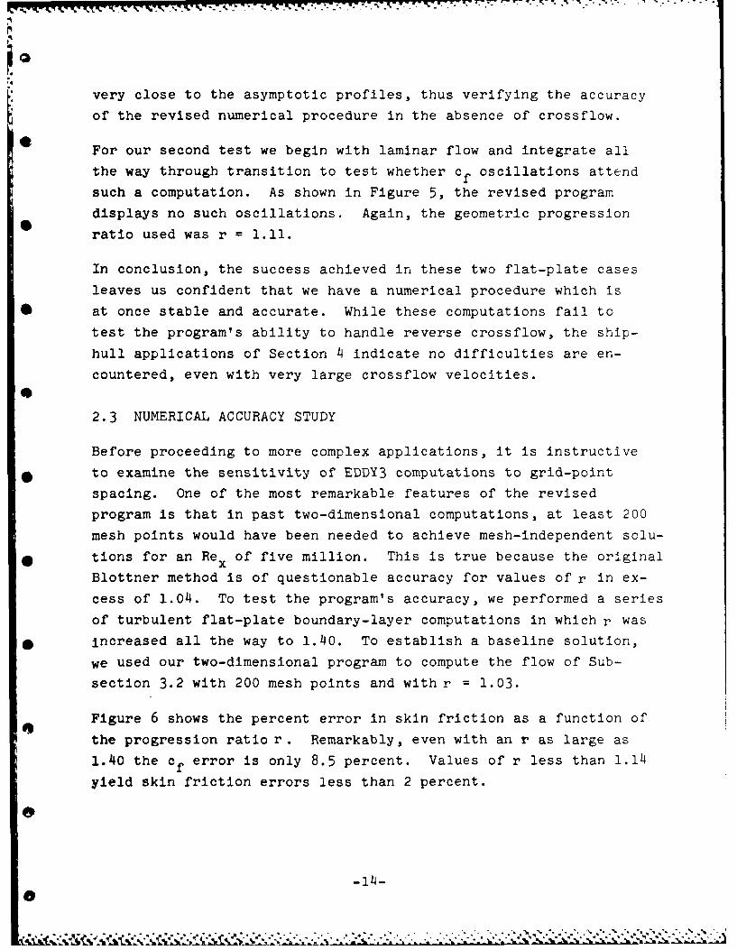
For our second test we begin with laminar flow and integrate all
the way through transition to test whether cf oscillations attend
such a computation. As shown in Figure 5, the revised program
displays no such oscillations. Again, the geometric progression
ratio used was r = 1.11.
In conclusion, the success achieved in these two flat-plate cases
leaves us confident that we have a numerical procedure which is
* at once stable and accurate. While these computations fail to
test the program's ability to handle reverse crossflow, the ship-
hull applications of Section 4 indicate no difficulties are en-
countered, even with very large crossflow velocities.
2.3 NUMERICAL ACCURACY STUDY
Before proceeding to more complex applications, it is instructive
* to examine the sensitivity of EDDY3 computations to grid-point
spacing. One of the most remarkable features of the revised
program is that in past two-dimensional computations, at least 200
mesh points would have been needed to achieve mesh-independent solu-
* tions for an Re x of five million. This is true because the original
Blottner method is of questionable accuracy for values of r in ex-
cess of 1.04. To test the program's accuracy, we performed a series
of turbulent flat-plate boundary-layer computations in which r was
* increased all the way to 1.40. To establish a baseline solution,
we used our two-dimensional program to compute the flow of Sub-
section 3.2 with 200 mesh points and with r = 1.03.
Figure 6 shows the percent error in skin friction as a function of
the progression ratio r. Remarkably, even with an r as large as
1.40 the c error is only 8.5 percent. Values of r less than 1.14
yield skin friction errors less than 2 percent.
0
-14-
. . .. .' . .*
Re 600
S - COMPUTED
400 0 BLASIUS
2000.
.06
0 0.5 1.0 1.5 2.0
10 5 Re.
.
CfFiur 5.__Comparison___ of__computed___and
~.008
-..-. 006
pont an r 1.1
5 - COMPUTED. ;0 BLASIUS
2 .02• KARMAN-• SCHOENHERR
S0 I
'...,0 0.5 1.0 1.5 2.0
,.. , 10 5 1e
*. Figure 5. Comparison of computed and,- ..- measured skin friction and• --- =momentum thickness for a
transitional flat-plateboundary layer; 148 mesh
r~j points and r~ 1 .11.
V ..

PERCENTERRORIN SKIN 10.0FRICTION
5.0
2.0S
1.0
0.5
0.2
.05 .10 .20 .50
(r -1)
Figure 6. Variation of skin frictionerror with geometric pro-gression grading ratio for
9 a flat-plate boundary layer.
* -16-
t" Figure 7 recasts the percent error in skin friction in terms of
.. mesh point number. As shown, solutions are more or less mesh
i independent beyond about60mhpons
-
. o°
,44-4
4417
.' ,,..4; ' , % '". -"2 ".. . " " ' "' ' ' ' " " "" .. '. ;. i '.
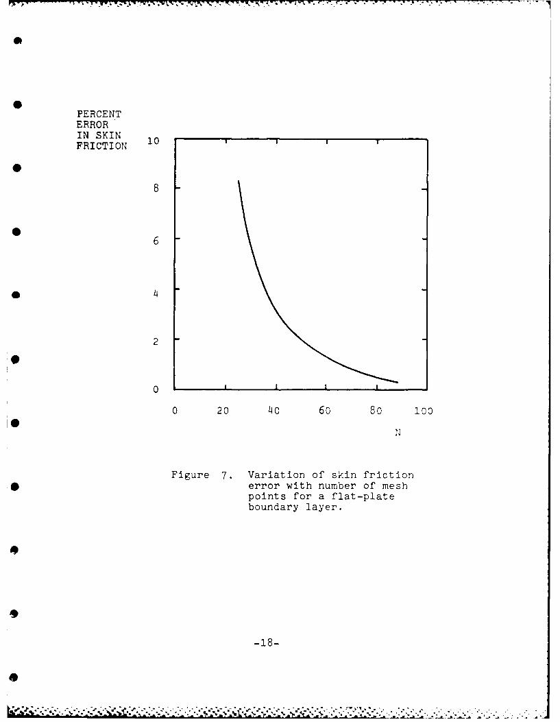
PERCENTERRORIN SKIN 10FRICTION i
8
6
* 4
2
0
0 20 40 60 80 100
U
Figure 7. Variation of skin frictionerror with number of meshpoints for a flat-plateboundary layer.
4
-18-
0
4. SHIP-HULL APPLICATIONS
We turn now to computation of the three-dimensional boundary layer
on two ship hulls, viz, the SSPA Model 720 and the HSVA Tanker.
These are the two test cases included in the 1980 SSPA-ITTC11Workshop on ship boundary layersl . For the SSPA Model 720 we
perform three separate computations to test EDDY3's ability to
handle reverse crossflow and sensitivity for grid point spacing.
Then, the HSVA Tanker computation is done just once on an optimized
grid.
The surface finite difference grid is nonorthogonal and PROGRAM
SHPMSH (see Section A.1 of the Appendix) is used to generate the
grid. Also, PROGRAM VELOC (see Section A.2 of the Appendix) is
used to interpolate inviscid velocities onto the nonorthogonal
grid.
4.1 SSPA MODEL 720
4.1.1 Effect of Girthwise Integration Direction
All of the computations performed use the Workshop-supplied Douglas-Neuman 1 2
Neumann1 inviscid velocity distribution. In all cases, computation
>2 is initiated from fully-turbulent boundary-layer profiles at 2x/L =
-0.6 (L is the hull half length). The profiles used match the
measured momentum thickness and skin friction. For the computations
of this Subsection, the finite-difference mesh consists of 51
equally-spaced points extending from 2x/L = -0.6 to 2x/L = 0.9,
11 equally-spaced points (in terms of girth) in the girthwise direc-
tion, and an average of 40 points normal to the surface. Thus, the
mesh consists of about 22,000 points. Consistent with the Douglas-
Neumann computation, both the keel line and the waterline have
been treated as symmetry planes.
To further test the program's numerical formulation, we perform
the computation in two different ways. First, we perform the
girthwise integration starting at the keel and integrating toward
the waterline on each streamwise plane (section). Then, we repeat
the computation integrating from waterline to keel. Doing both
-19-
2computations checks numerical-algorithm consistency and the pro-
gram's ability to handle reverse crossflow.
Inspection of key flow properties shows virtually no difference
between the two solutions through the entire flowfield. This
confirms that the program is indeed able to handle reverse cross-
* flow in a stable and accurate manner. It also confirms that over-
all the algorithm is consistent witi. the parabolic nature of the
boundary-layer equations.
4.1.2 Effect of Mesh Refinement
In the next computation we use 81 mesh points in the streamwise
direction, half of which lie between 2x/L = 0.5 and 2x/L = 0.9.
A total of 21 equally-spaced points lie in the girthwise direc-
tion with an average of 75 points normal to the surface. This
mesh consists of about 128,000 points, almost six times the
number used in the computations of Subsection 4.1.1. The girth-
wise integration is carried out from keel to waterline.
A detailed comparison of corresponding flow properties for the
22,000- and the 128,000-mesh-point computations shows that over-
all flow properties differ by about 3 percent. Even in regions
* of rapid change, differences never exceed 5 percent. These ob-
servations are consistent with our accuracy study for the flat-
plate boundary layer which indicate that, on the one hand, using
40 points normal to the surface yields a little over 3 percent
* error while, on the other hand, using 75 points results in about
0.6 percent error. The 5 percent discrepancies almost certainly
attend the difference in streamwise resolution between the two
computations.
Results of this numerical test indicate there is little point in
using a mesh as fine as the one with 128,000 points if economy
is a factor. That is, our 22,000-point computations require ap-
* proximately 20 minutes on a UNIVAC 1108 while the 128,000-point
computation requires about 90 minutes. Note that the increase
-20-

in machine time is slower than linear because use of the finer
.- mesh is attended by fewer iterations in the solution procedure
at each mesh point.
4.1.3 Comparison of Computed and Measured Momentum Thickness
In all three computations, we predict boundary-layer separation
over a portion of the hull beyond 2x/L = 0.77. Although no sep-
aration appears to have been observed experimentally, one should
also note that the experimentally observed boundary layers did
not experience as strong an adverse pressure gradient as those
*predicted by the Douglas-Neumann computation.
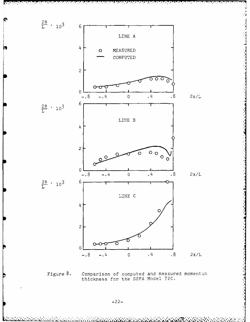
Figure 8 compares computed and measured momentum thickness, e,
on three lines along the hull. Line A is the keel line. Line B
is a line well below the waterline where the boundary layer is
more-or-less of the classical "thin" variety. Line C is closer
to the waterline and the boundary layer approaches the more com-
plicated "thick" structure.
Along Line A, the boundary layer is truly three dimensional as
exhibited by its curious behavior approaching the stern. Speci-
fically, despite entering a region of adverse pressure gradient,
the momentum thickness decreases. This behavior occurs because
of large flow divergence near the stern. While the computed 0
lies about 25 percent above measured values, note that our pre-
dicted curve is much closer to the data than those of virtually
all Computors in the SSPA-ITTC Workshop on Ship Boundary Layers,
most of whose curves were high by a factor of two!
Along Line B, we exhibit somewhat larger differences from the
measured values. Computors in the Conference generally came
closest to experimental data on this line. Our prediction is
about average relative to Conference participants'.
-21-
2 03 6 I
LINE Aj
0 MEASURED
- COMPUTED
2
000
-.8 -.4 0 .4.8 2x/L
LINE B
4
20 00
00o I I0
-. 8 -. 4 0 .4 .8 2x/L
2e 103 6
LINE C
4
010
-.8 -.4 0 .. 8 2x/L
Figure 8. Comparison of computed and measured momentum~thickness for the SSPA Model 720.
-22-
On Line C, our predicted curve follows measured values quite
closely up to about 2x/L = 0.5; beyond this point we predict a
slower-than-measured increase in momentum thickness. This is
unsurprising as no provision has been made to accomodate any
"thick" boundary-layer phenomena. Our prediction is much closer
-' to the data than most Conference participants'.
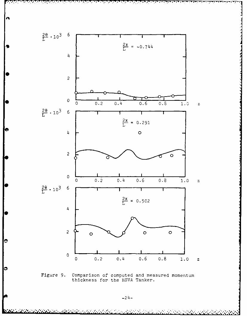
4.2 HSVA TANKER
As with the SSPA Model 720, we use the Workshop-supplied Douglas-
Neumann inviscid velocity distribution. Computation is initiated
from fully-turbulent boundary-layer profiles at 2x/L = -0.80. Again,
the profiles used match the measured momentum thickness and skin
friction. The finite-difference mesh consists of 70 points in the
streamwise direction extending from 2x/L = -0.80 to 2x/L = 0.90,
15 equally-spaced points (in terms of girth) in the girthwise
direction, and an average of 60 points normal to the surface. Figure
9 compares computed and measured momentum thickness on three sections,
viz, for 2x/L = -0744, 0.291 and 0.502. The numerical boundary
layer separated over a substantial portion of the hull at 2x/L = 0.75,
so that comparison with momentum-thickness data at 2x/L = 0.884 is
not possible. Note that the abscissa, z, is the nondimensional
girth with z=0 on the keel and z=l on the waterline. Overall
differences between computed and measured 6 are similar to those
obtained for the SSPA Model 720.
In summary, we have tested EDDY3 on two ship hulls and encountered
no significant numerical difficulty. Separation on both hulls is
almost certainly caused by the use of the Neumann inviscid velocities,
so separation is discounted as a numerical problem. The differences
observed between computed and measured momentum thickness, although
generally much smaller than those of Workshop participants, are
too large for general engineering applications. Thus, our predictive
ability requires further improvement before a ship designer can
apply a program such as EDDY3 with any degree of confidence.
k"
-23-
..........................................
2x - 0-4
'4
2
* 0 0 .2 0.~4 0.6 0.8 1.0 z
2e 103 6
2x--0.291
'4 0
2
00
0 0.2 o.'4 0.6 0.8 1.0 z2 9 i10 3 6 1 I IL
-0502
00
00 0.2 o.14 0.6 0.8 1.0 z
Figure 9. Comparison of computed and measured momentumthickness for the H-SVA Tanker.
-24-

Inspection of Figures 8 and 9 indicates our predictions differ
from measurements most significantly as we approach the stern.
This is unsurprising because, on the one hand, we expect the
boundary layer to become "thick" so that classical thin-shear-layer
approximations become suspect while, on the other hand, our compu-
tations have been done with classical thin-shear-layer approxima-
tions. In the next section, we address the question of how well
our model equations predict properties of "thick" boundary layers
if we abandon the thin-shear-layer limit.
S-25
NIr.
...
-.
.'. -2 5-
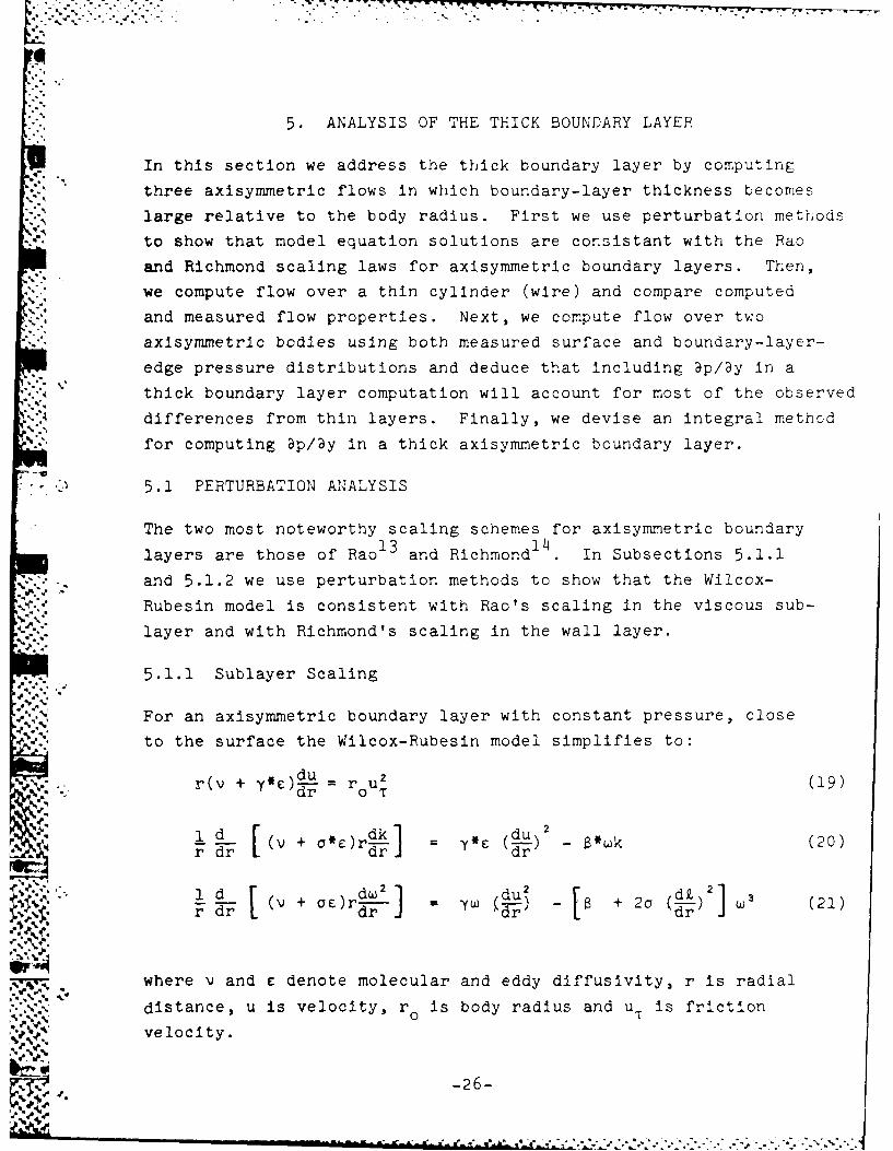
5. ANALYSIS OF THE THICK BOUNDARY LAYER
In this section we address the thick boundary layer by computing
three axisymmetric flows in which boundary-layer thickness becomes
large relative to the body radius. First we use perturbation methods
to show that model equation solutions are cornsistant with the Rao
and Richmond scaling laws for axisymmetric boundary layers. Then,
we compute flow over a thin cylinder (wire) and compare computed
and measured flow properties. Next, we compute flow over two
axisymmetric bodies using both measured surface and boundary-layer-
edge pressure distributions and deduce that including ap/ay in a
thick boundary layer computation will account for most of the observed
differences from thin layers. Finally, we devise an integral method
for computing ap/3y in a thick axisymmetric boundary layer.
5.1 PERTURBATION ANALYSIS
The two most noteworthy scaling schemes for axisymmetric boundary
layers are those of Rao1 3 and Richmond In Subsections 5.1.1
and 5.1.2 we use perturbation methods to show that the Wilcox-
Rubesin model is consistent with Rao's scaling in the viscous sub-
layer and with Richmond's scaling in the wall layer.
5.1.1 Sublayer Scaling
For an axisymmetric boundary layer with constant pressure, close
to the surface the Wilcox-Rubesin model simplifies to:
r(v + u)du = r u2 (19)1 ddk
.4 d( v + = y du 2 -"wk (20)FrT dr di r
drF(v + acrw du2 + 2a (1 W (21
where v and c denote molecular and eddy diffusivity, r is radial
distance, u is velocity, r is body radius and uT is friction
N, velocity.
-26-
M., TF.IF-777. -7.
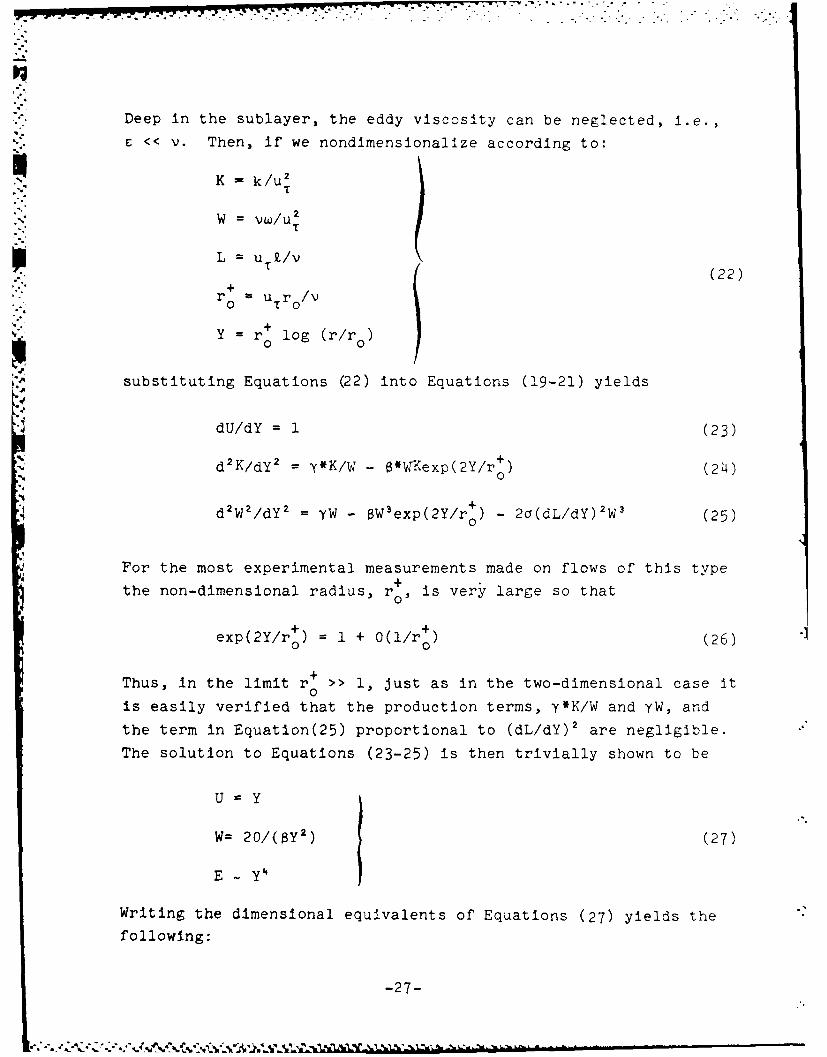
Deep in the sublayer, the eddy viscosity can be neglected, i.e.,
C << v. Then, if we nondimensionalize according to:
K = k/ut
W = VW/u
L = u T/v(22)
+0 UTro/
+ lo r/ oY = 0 log (r/r0)
substituting Equations (22) into Equations (19-21) yields
dU/dY = 1 (23)
d2K/dY 2 = y*K/W - e*WKexp(2Y/r ) (24)0
2 W2 /dy2 yW - aW 3exp(2Y/r ) - 2a(dL/dY) 2W3 (25)
4For the most experimental measurements made on flows of this type
the non-dimensional radius, r0 , is very large so that
exp(2Y/r) = 1 + 0(1/r ) (26)
Thus, in the limit r+ >> 1, Just as in the two-dimensional case it
is easily verified that the production terms, y*K/W and yW, and
the term in Equation(25) proportional to (dL/dY)2 are negligible.
The solution to Equations (23-25) is then trivially shown to be
U= Y
W= 20/(SY 2 ) (27)
E ~y4
Writing the dimensional equivalents of Equations (27) yields the
following:
-27-
... . ..-.,. i~f vr.1 , -%.
|if 77.- 7")
u/u = r+ log(r/r oI.T 00
VW/u 2 20v/IB(log r4)2 (8+ r (8
k/u' (ro+log r-)4
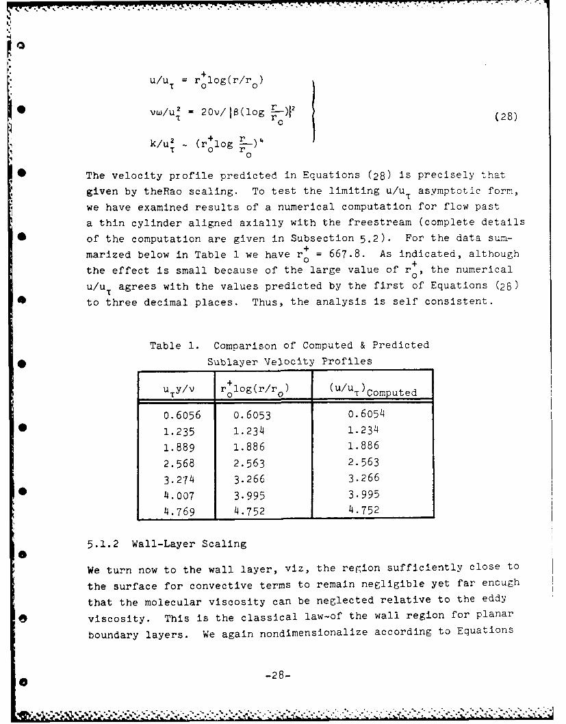
* The velocity profile predicted in Equations (28) is precisely that
given by theRao scaling. To test the limiting u/u asymptotic form,
we have examined results of a numerical computation for flow past
a thin cylinder aligned axially with the freestream (complete details
* of the computation are given in Subsection 5.2). For the data sum-+
marized below in Table 1 we have r0 = 667.8. As indicated, althougho+
the effect is small because of the large value of r0 , the numerical
u/u T agrees with the values predicted by the first of Equations (28)
* to three decimal places. Thus, the analysis is self consistent.
Table 1. Comparison of Computed & Predicted
* Sublayer Velocity Profiles
u Y/v r+ log(r/r) (u/U )T______ o o T Computed
0.6056 0.6053 0.6054
* 1.235 1.234 1.234
1.889 1.886 1.886
2.568 2.563 2.563
3.2-74 3.266 3.266
* 4.007 3.995 3.995
4.769 4.752 4.752
5.1.2 Wall-Layer Scaling
We turn now to the wall layer, viz, the region sufficiently close to
the surface for convective terms to remain negligible yet far enough
that the molecular viscosity can be neglected relative to the eddy
O viscosity. This is the classical law-of the wall region for planar
boundary layers. We again nondimensionalize according to Equations
-28-
iv . v °.W V V %".,V% -" "y.-*'".". "2. ".'.' o ,....- . ." '". . " " """ . "-- "." "°.- .... " . - . . - ..
-7:-7 -- :
(22) with the exception that our normal coordinate is redefined as
follows.
Y = Y+(1 + y /r ) where y = (r - r ) (29)0 0
The wall layer is most conveniently analyzed by treating U as the
dependent variable. Dropping molecular viscosity in Equations
(19-21)i the equations for the wall layer are:
(1 + 2Y/r ) (K/W)dU/dY = 1i ,g0q (30)
a*d2 K/dU 2 = a*(l + 2Y/r )K2 - 10 ~(31)
ad W2 /dU 2 = a(l + 2Y/r+)KW2 - yW2 /K + 2o(dL/dU)2 W'/K (32)
In the limit of very large r+ these equations are identical to those0
for planar boundary layers. From Equation (31) there follows
immediately:
E = 1//- + 0(1/r 0) (3)
Substituting Equation (33) into Equation (32), the solution for W
becomes (noting that the closure coefficients have been chosen to
insure that y =61/ - 20K 2 //a where K is Karman's constant):
W exp(- KU)K = <--- (34)
Finally, substituing Equations (33-34) into Equation (30 )yields
the velocity profile, viz,
=U lY + 0(1/r ) (35)K 0
or in dimensional form we have:
u/u i logy+ + (36)
where
-29-
-. 4-°
~++
Y = y (1 + y /2r o) (37)
Equations (36-37) are precisely those of the Richmond scaling.
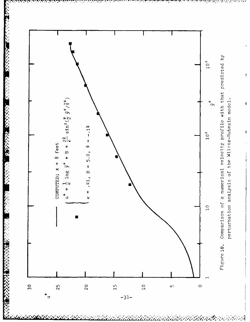
In Figure I we compare our numerical predictions for the thin clinder
computation of the next subsection with Equations (36-37). In the
comparison we have included Coles' wake component so that the complete
velocity profile becomes:
Tu = 1 log + + B + 2i sin2(T ) (38)T K K 2-4
where we use K = .41, B = 5.0 and = -.14. Note that the inferred
wake strength i of -.14 implies that the transverse curvature effect
* is similar to a favorable pressure gradient. This point is consistent
with the observations of Patel1l The overall agreement between the
numerical profile and Equation (38) verifies the perturbation analysis.
5.2 FLOW PAST A WIRE
In this subsection we present results of a numerical computation for
flow past a "wire", viz, a thin cylinder aligned axially with the
freestream. The case we have chosen is that experimentally investi-
gated by Yulin which the Reynolds number based on cylinder radius is
Re = 15,250 (39)
• Unit Reynolds number for the flow is 1.83105 and measurements were
made between axial distances, x, from 2 feet to 8 feet. At x = 8
feet the ratio of boundary layer thickness to r0 is approximately 2
so that this flow includes a moderately "thick" boundary layer.
Computation was initiated at x = 0 from laminar starting conditions.
The freestream turbulence intensity was adjusted to yield a match
between computed and measured momentum thickness at x = 2 feet.
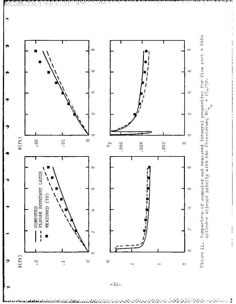
* Figure 11compares predicted boundary layer thickness, 6, momentum
thickness, e, shape factor, H, and skin friction, cf, with corres-ponding measurements. The data shown for 6, e, and H are the original
-30-
44-
.0
4-A
aQ -H
00 +
4.)
it ++ 4.
0 0
E- 4A ) 0HE t
0 +H
0.
0) 4) C)i
0) *H -4
0) *H
00
LC\G)
OD CC) C7
0 cli
I CD
Oj -1C )~
0~ I- \1 -iC
4-.
Ic ) Co
P. 77. C/) Lo)
CC
CDC
r-CA CD
CD -4
-32-

data reported by Yu. The skin friction data have been obtained from
Clauser plots rather than using Yu's Preston tube measurements which
are thought to be in error1 5 .
As shown, computed and measured shape factor and skin friction differ
* by less than 5%. Computed boundary-layer thickness is about 10%
* lower than measured while the numerical momentun thickness ultimately
%] is about 15% lower than measured. The fact that our skin friction
is so close to the measured values while the momentum thickness
discrepancies are much larger leaves us with the same concern exores-
sed by Patel 7 regarding the two-dimensionality of the experimental
flowfield. The figure also shows computed results for a corresponding
planar boundary layer. As indicated, the primary effects of transverse
curvature are to increase skin friction and momentum thickness and to
decrease boundary-layer thickness and shape factor.
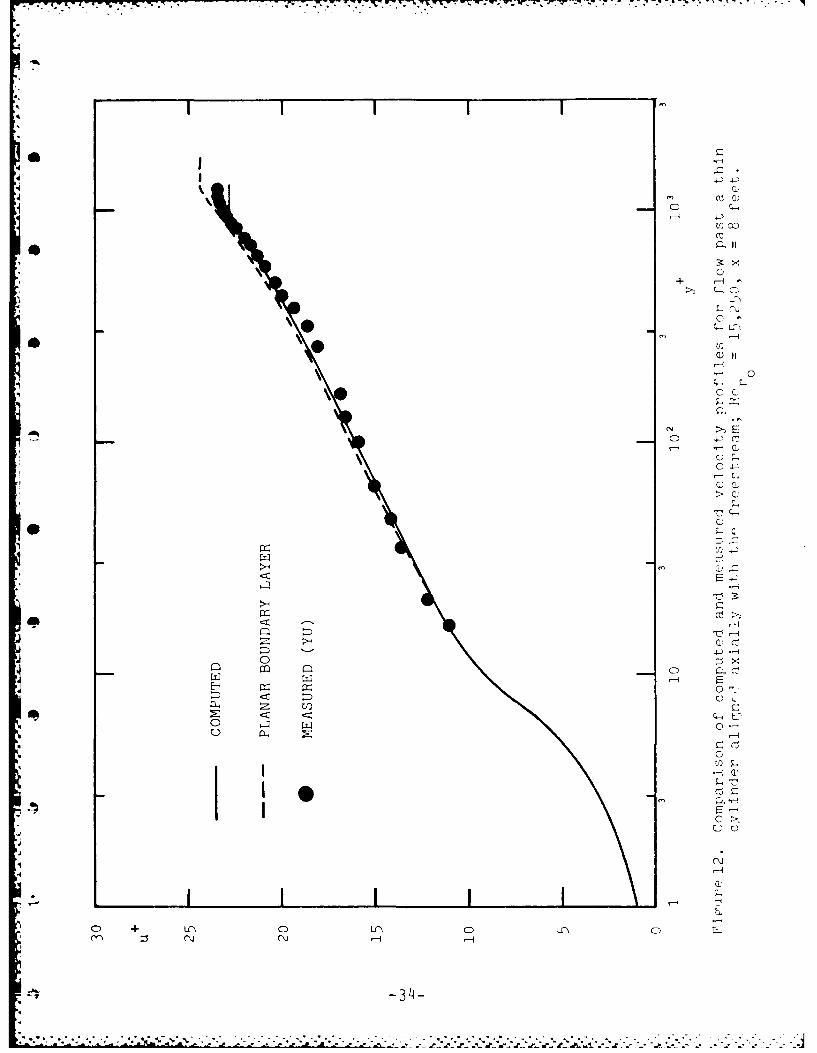
Figure 12 compares the computed and measured velocity profiles at the
axial location x = 8 feet. With exception of the points lying between
Y+ = 150 and 400, the computed velocity profile fares smoothly through+
the data. Even for the four data points lying between y = 150 and400, the maximum difference is less than 5%. Inspection of the
profile for the corresponding planar case shows that the effect of
transverse curvature is to alter the slope of the profile, a trend
consistent with that displayed in the data.
Thus, for this constant-pressure flow, the model equations pre-
dict flow properties which are reasonably close to corresponding
measurements. As will be seen in the next subsection, thick
boundary layers experiencing an adverse pressure gradient cannot
be as accurately computed if we restrict ourselves to classical
thin-shear-layer approximations.
-33-
I . .. -.... . ., . . . . ..- . - -, . . . . . , - .,. -. -. - . ... . . .. . .
-)
4 C)
CD-
* Q: II
CD C
0
C))I
-4
0
CD UU C C
CCC)
-34-)
.. ° -. o"
5.3 BODIES WITH ADVERSE PRESSURE GRADIENT
In this Subsection, we make a "first cut" at two thick axisymmetriLc
boundary layers with pressure gradient and streamline curvature.
We emphasize that our computations are indeed only a first cut as
S.. experimental measurements indicate nontrivial variation in pressureacross the boundary layers while we have used a standard boundary-
layer program which assumes Dp/3y = 0. In order to provide a first
estimate of the importance of having variable pressure across the
layer, we have done both computations first using the measured edge-
*. pressure distribution and then with the measured surface-pressure
distribution.
The two cases considered are the "modified spheroid"l8 and the
"low-drag body ' 1 9 experimentally evaluated by Patel. In Subsection
5.3.1 we compare computed and measured integral properties. Sub-
section 5.3.2 compares computed and measured velocity and Reynolds
" shear-stress profiles for the low-drag body. Next, in Subsection
.5.3.3, we compare predicted peak eddy viscosity and mixing length
with corresponding measurements. Finally, Subsection 5.3.4 examines
the predicted effect of streamline curvature for the modified
spheroid.
5.3.1 Integral Properties
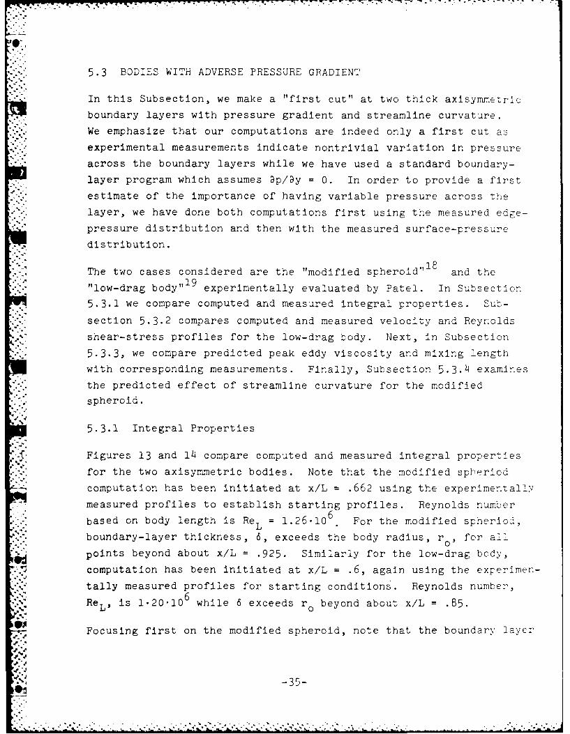
Figures 13 and 14 compare computed and measured integral properties
for the two axisymmetric bodies. Note that the modified spberiod
computation has been initiated at x/L = .662 using the experimentally
measured profiles to establish starting profiles. Reynolds number
based on body length is Re = 1.26.10 6 For the modified spheriod,Lboundary-layer thickness, 6, exceeds the body radius, r , for all
points beyond about x/L = .925. Similarly for the low-drag body,
computation has been initiated at x/L = .6, again using the experimen-
tally measured profiles for starting conditions. Reynolds number,"-" 06, Re is 1.2010 while 6 exceeds r beyond about x/L = .85.
L 0
Focusing first on the modified spheroid, note that the boundary layer
.4 -35-
. °° -, .
co 0::D I C-~
0
CC.
0~ 0
0@ C)
Q)
C- C) UCC)f' D L C m Cj rA C
m N C i -CD C C)0C CD -
C) C) (D C CD C)A C D CD C D C
__ _ _ _ _ _ _ _'0 C) C ) C ) C
I 4.4
0 0
0Cl 0
* C00c0 cc
C)'.
00C
00 0 c CCD CD CD- CD
0 0-36-

CQ 0
I Q)
0 0
12L4)
CC o 0
;.4 C C > C )cl
C) C)
01)
N. 0 0 0 .. C) Q 0 0 E C.)
CC 00 0
C
0 <
\4 00 -j ) 0 \D -- Q C
C CD 0 0 CD C
N- C-
o ~-37)
II II
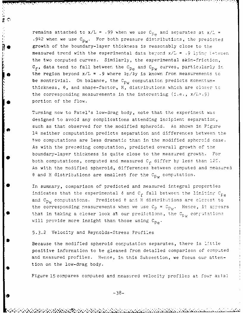
Wiremains attached to x/L .99 when we use Cpe and separates at x/L =
.942 when we use C pw* For both pressure distributions, the predicted
•growth of the boundary-layer thickness is reasonably close to the
measured trend with the experimental data beyond x/L = .9 lyin - et.ee
the two computed curves. Similarly, the experimental skin-friction,
* Cf, data tend to fall between the Cpe and Cpw curves, particularly in
* the region beyond x/L = .9 where 9p/ay is known from measurements to
be nontrivial. On balance, the CPw computation predicts momentum-
thickness, e, and shape-factor, H, distributions which are closer to
the corresponding measurements in the interesting (i.e., x/L>.9)
* portion of the flow.
Turning now to Patel's low-drag body, note that the experiment was
designed to avoid any complications attending incipient separation,
such as that observed for the modified spheroid. As shown in Figure
14 neither computation predicts separation and differences between the
two computations are less dramatic than in the modified spheroid case.
As with the preceding computation, predicted overall growth of the
boundary-layer thickness is quite close to the measured growth. For
both computations, computed and measured Cf differ by less than 12'.
As with the modified spheroid, differences between computed and measured
e and H distributions are smallest for the Cpw computation.
* In summary, comparison of predicted and measured integral properties
indicates that the experimental 6 and Cf fall between the limitinE Cpe
and Cpw computations. Predicted e and H distributions are clcest to
the corresponding measurements when we use Cp = Cpw. Hence, it appears
* that in taking a closer look at our predictions, the Cpw cov.putations
will provide more insight than those using Cpe'
5.3.2 Velocity and Reynolds-Stress ProfilesS
Because the modified spheroid computation separates, there is little
positive information to be gleaned from detailed comparison of computed
and measured profiles. Hence, in this Subsection, we focus our atten-
tion on the low-drag body.
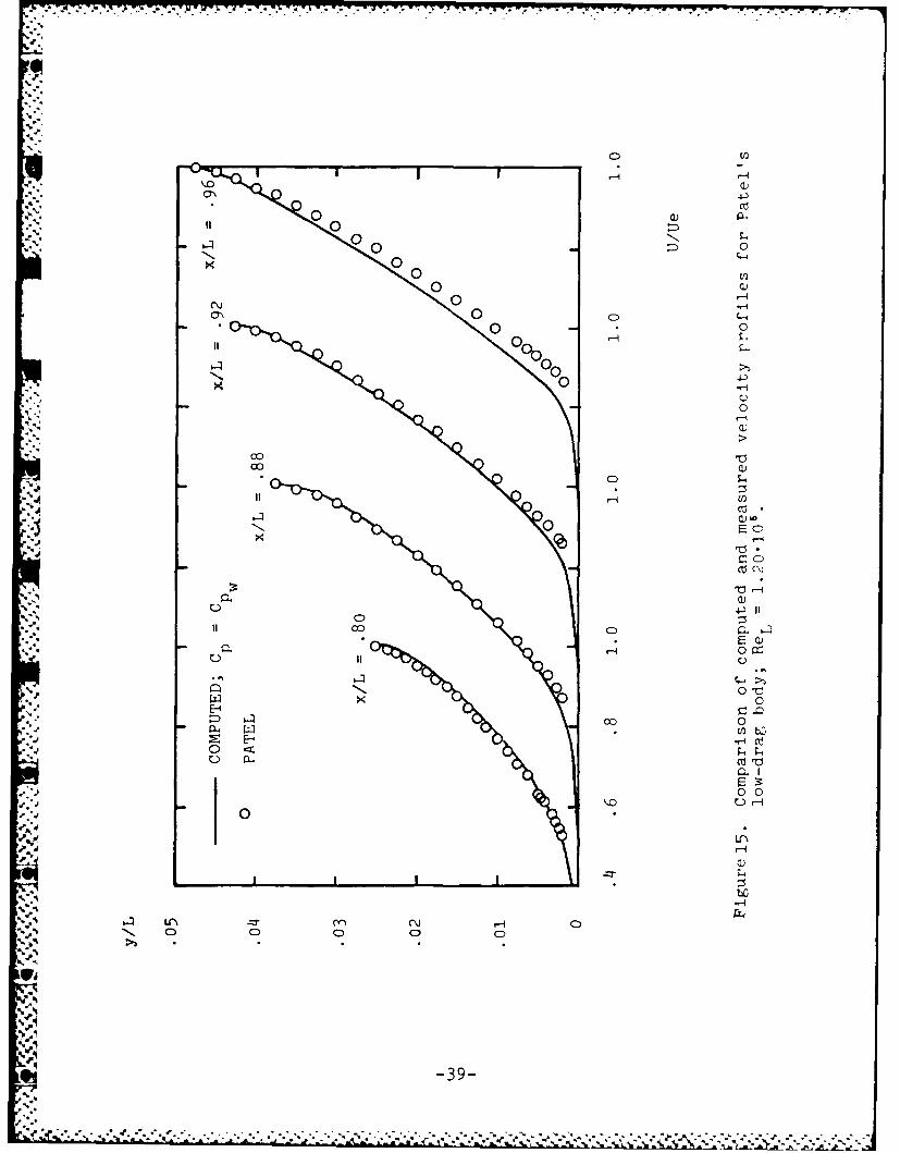
Figure 15 compares computed and measured velocity profiles at four axial
-38-
' '-. .% ;- -'-..- .' ' .--:'-)- ." -.-" -.b--:. -:., " -,-:-."---:" .",:- ( :-- (k---;. .: .. .. . .: b
- 77 . .
A-'i
00
0 C)-
0 co0 0
00 C-
0000
ii 000
00
A.o
r-i U)
C \
CC) C)
0l
01
E-40
0 ow -4
N~~ 0
L '
4
.A..*4.A.*'.*. -'- .. *~A A*'A*~*~A* * .A-39-*. *

stations, viz, x/L = .80, .88, .92, .96. As shown, the computed
boundary layer has experienced stronger deceleration than in the
experimental case. This is unsurprising as we have used the surface-
pressure distribution throughout the layer which is attended by a
larger gradient. Clearly, the overall growth matches that measured.
Even at x/L = .96, differences between computed and measured velocities
are less than 7% of scale.
Figure 16 compares computed and measured Reynolds shear-stress profiles.
Discrepancies between the profiles at x/L = .80 are surprising, parti-
cularly in the light of the close agreement between the velocity
* profiles at this station. Overall, the numerical shear-stress profiles
are within about 15% of scale of the measured profiles. The shapes
and fullness of the experimental profiles are reasonably well simulated
throughout the tail region of the body.
5.3.3 Turbulence Properties
In this subsection we concentrate on two key features of the turbulence
field which have not been accurately simulated with simpler turbulence
0 models. Specifically, we examine the variation of peak mixing-length,
zmax' and eddy viscosity, cmax' Figure l7compares our CPw predictions
with values inferred from Patel's data. As shown, for both bodies,
model-predicted £ and e fall off rapidly as we approach the tail•max max
of the body. Considering the inaccuracies attending differentiation
of the experimental data required to infer kmax and max' our predic-
tions must be considered well within the error band of the data.
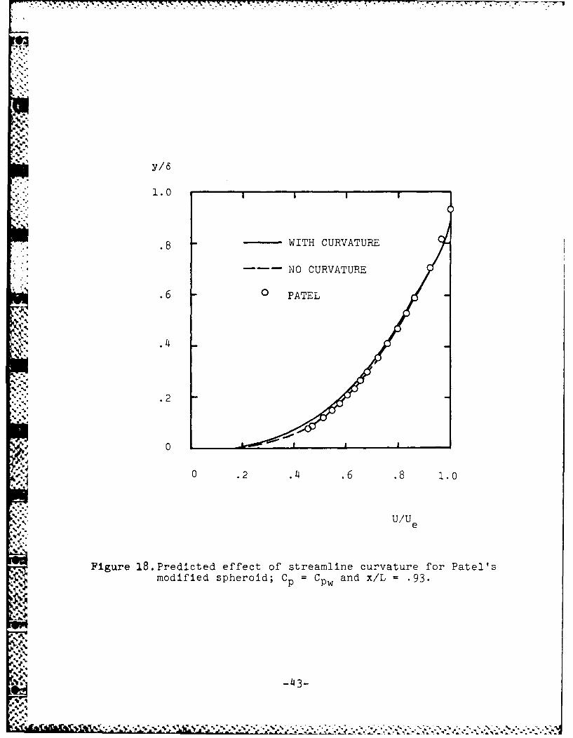
• 5. 3 .4 Streamline-Curvature Effects
To obtain an estimate of the effects of streamline curvature on our
predictions, we have rerun the Cpw modified-spheroid computation
* without account for streamline curvature. All results presented in
Subsections 5.3.1-5.3.3 include the Wilcox-Chambers2 0 curvature modi-
fication to the turbulent mixing-energy equation. Figure 18 shows effectz
on the velocity profile at x/L = .93. For the computation with no
* curvature, the numerical profile passes through all of the measured
points. With curvature included, the velocity profile shows additional
deceleration, consistent with the effect of convex curvature. Note
..-............. ........................ , . ,-,.......

.-,, il-
y/L
I..) .05
- COMPUTED, C p C px/L =.96
.40 PATEL 0 9
x/L .88.03
x/L= .80 000
.02 0 000 0
0,0 0 0
0 0
.01 0 O
0 -
0 .0002 .0008 o00 ooo8 .0008
<u v
S0.
Figure 16. Comparison of computed and measured Reynolds shear-stressprofiles for Patel's low-drag body; ReL - 1.20.106.
-41-
* * ---.. . . . .. .

I~T I C-
db0 -40
0 x 1
* 0~* >- S 000
1100c
Ir C~ 0 \ -T C D EmCE C) C C
CQ m
E
'C C L
X CC
Cd C).
co
0 C E
00 .0
0 -00 CC)
0 0'
rLU -4-)
0d
9b '0
* 0
0 H 0C0
-42
. ....-. .-. . . . -
S. . .. - -
1.0
.8 WITH CURVATURE
NO CURVATURE
.6 O PATEL
4.4
.2
0 0
0 .2 .4 .6 .8 1.0
U/U
Figure 18.Predicted effect of streamline curvature for Patel'smodified spheroid; Cp = Cpw and x/L - .93.
-43-
that the close agreement between results of the no-curvature computa-
tion and the experimental data is fortuitous as the numerical pressure
* gradient is larger through much of the boundary layer than it is in
the experimental case. Overall, the effect of curvature for the
modified spheroid is small, giving rise to changes in integal pro-
perties of less than 5%
In summary, results of these two computations indicate the
*' following.
1. With no modifications to the Wilcox-Rubesinturbulence model, computed boundary-layer
*0 thickness virtually duplicates measuredthickness for both bodies.
2. Performing the computations with first themeasured boundary-layer-edge pressure
* distribution and then with the measuredsurface pressure distribution (neglectingpressure variation across the layer in eachcomputation) yields skin-friction distribu-tions which overall fall above and belowmeasured skin friction, respectively.
3. Shape factor and momentum thickness are in
closer agreement with corresponding measure-ments when the wall pressure is used.
S4. For one of the two bodies, our predictions
suggest that streamline curvature plays arelatively minor role.
Thus, we conclude that the primary differences between the "thick"
* and the "thin" boundary layer are primarily caused by the pressure
gradient across the former, i.e., Dp/3y. In the next Subsection,
we devise a straightforward method for including 3p/ay in a standard
boundary-layer computation.
5.4 PRESSURE VARIATION IN A THICK BOUNDARY LAYER
Results of the preceding Subsection demonstrate the importance of
pressure variations across a thick axisymmetric boundary layer.
Recapitulating, we found that in using a conventional boundary
~-~.-44-
. ~ .-. .*-*- - . .- ~ *. * .. . -i *:. . *
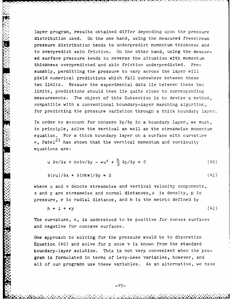
layer program, results obtained differ depending upon the pressure
distribution used. On the one hand, using the measured freestream
pressure distribution tends to underpredict momentum thickness and
to overpredict skin friction. On the other hand, using the measur-
ed surface pressure tends to reverse the situation with momentum
thickness overpredicted and skin friction underpredicted. Pre-
sumably, permitting the pressure to vary across the layer will
yield numerical predictions which fall somewhere between these
two limits. Because the experimental data lie between these two
limits, predictions should then lie quite close to corresponding
measurements. The object of this Subsection is to devise a method,
compatible with a conventional boundary-layer marching algorithm,
for predicting the pressure variation through a thick boundary layer.
In order to account for nonzero 3p/3y in a boundary layer, we must,
in principle, solve the vertical as well as the streamwise momentum
equation. For a thick boundary layer on a surface with curvature
K Patel2 1 has shown that the vertical momentum and continuity
equations are:
u 3v/Dx + hv~v/3y - (40)
P
a(ru)/Dx + 3(rhv)/Dy = 0 (41)
where u and v denote streamwise and vertical velocity components,
x and y are streamwise and normal distances,p is density, p is
pressure, r is radial distance, and h is the metric defined by
h h1+Ky (42)
The curvature, K, is understood to be positive for convex surfaces
and negative for concave surfaces.
One approach to solving for the pressure would be to discretize
Equation (40) and solve for p once v is known from the standard
boundary-layer solution. This is not very convenient when the pro-
gram is formulated in terms of Levy-Lees variables, however, and
all of our programs use these variables. As an alternative, we have
....................................
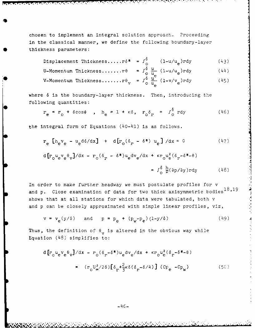
chosen to implement an integral solution approach. Proceeding
in the classical manner, we define the following boundary-layer
thickness parameters:
Displacement Thickness ..... r6* = f6 (1-u/U )rdy (43)0 e
U-Momentum Thickness ....... r6 = f6 (1-u/u )rdy (414)
V-Momentum Thicknessu.......rev o6 (1V/Ve )rdy (45)
where 6 is the boundary-layer thickness. Then, introducing the
following quantities:
0 6r r + 6cos€ h = 1 + K6, r 6 = f0 rdy (46)re= 0 e o r0
the integral form of Equations (40-41) is as follows.
re [hev e - U ed6/dx] + d[r (6r - 6") U e] /dx = 0 (47)
doeev]/dx - ro( r -*)Uedve/dx + Krou e *-e)
f h (ap/3y)rdy
In order to make further headway we must postulate profiles for v18,19and p. Close examination of data for two thick axisymmetric bodies
shows that at all stations for which data were tabulated, both v
and p can be closely approximated with simple linear profiles, viz,
v = v (y/6) and P = Pe + (pw-Pe)(l-y/6 ) (49)e ee
Thus, the definition of 0 is altered in the obvious way whilev
Equation (48) simplifies to:
dro/dx - r(6 6*)U dV/dx + rou'(6 r6*-e)
Lrouevevx r r e ve oe(6
(roUt,/26)[ 6 +3K6(6-6/4)] (Cp CP (5:
-46-
.. . .. . . . . . . .

* In order to test this formulation, we have applied Equations (L47Sand 50) to three flows, in each case working with measured flow
16properties. The three cases are Yu's flow over a wire, Patel's
modified spheroid 18 and Patel's low-drag body 19, respectively.
For Yu's wire flow, we find that the difference between edge and
surface pressure coefficients is of order 10- , as would be ex-
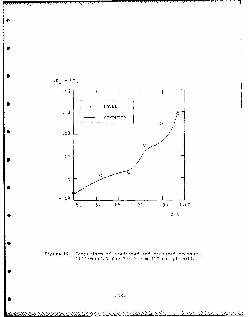
pected for this constant pressure case. Figures 19 and 20 compare
predicted and measured pressure coefficient difference for the
.vtwo Patel bodies. Considering the numerical crudeness attending
differentiation of the data, particularly v the agreement
" between the predictions of Equation (50) and the measured C~pdifference is excellent.
Note that Equations 47 and 50 are not restricted to axisyr.metric
boundary layers. The limiting two-dimensional forms fcllow by
- formally replacing re by r° and 6 by 6. The equations can tee 0 rgeneralized in a straightforward manner for three-dimensional
boundary layers.
-47
-wmo"
'S.<
!"7
Cpw - Cp6
.16
. 0 PATEL
.12 - -
COMPUTED0
* .08-
o8o
0
000 0
-. o4 II I
.80 .84 .88 .92 .96 1.00
* x/L
Figure 19. Comparison of predicted and measured pressuredifferential for Patel's modified spheroid.
-48-
.. . ..B . ..

Cp - Cp
.o8
o06 0 PATEL
CO MP UTE D
0
0
020
00 0
000
-. 020
-. 04I I
.50 .60 .70 2.0 10
Figure 20. Com-arison of predicted and Treasured pressuredifferential for Patel's low-drag body.
Pd -149-
. .- i .06
6. DISCUSSION
1 We have developed a new three-dimensional boundary-layer program,
EDDY3, suitable for application to arbitrary ship hulls. The pro-
gram embodies the Wilcox-Rubesin two-equation turbulence model and
uses an accurate, efficient numerical procedure based on the Blot-
tner "variable-grid" method coupled with the Krause explicit mar-
ching algorithm.
Results described in Sections 3 and 4 show that very accurate num-
0 erical results can be obtained with relatively coarse finite-dif-
ference grids. Computing times are quite modest as a complete shiphull computation can be done with about a half-hour of UNIVAC 1108
execution time. This corresponds to approximately three minutes on
a CDC 7600 computer. Additionally, the numerical algorithm dis-
plays no noticible difficulty when reverse crossflow is present.
Comparison of computed and measured flow properties for the SS7A
*O Model 720 and the ESVA Tanker show that, on the one hand, our Ere-
dictions are quite a bit closer to measurements than those repcrted
in the 1980 SSPA-ITTC Workshop on Ship Boundary Layers. On the
other hand, differences are too large, particularly near the ship
O stern, for us to claim the problem is solved. The fact that the
boundary layer becomes "thick" approaching the stern is no doubt
the cause of the differences observed between theory and experiment.
o Our analysis of thick axisymmetric boundary layers in Section 5
shows that, in order to obtain accurate "thick" boundary-layer pre-
dictions, accounting for the normal pressure gradient, 3p/Dy,
probably is all that is needed above and beyond conventional thin-
40 shear-layer approximations. Streamline curvature variation appears
to play a relatively minor role in the "thick" boundary layer.
Additional research is needed to confirm the importance of n in
ship-hull computations. The formalism developed in Subsection . '
-50-
. .. , ' ' , , . .- . .. . ...--.... . .. -. . ., _ . ,.. .

LT R--
can be easily generalized for a 3-D boundary layer and should be
included in EDDY3. We could then repeat the two ship-hull comr-
putations of Section 14 to confirm our hypothesis. Additionall,,
it would be instructive to use measured freestream flow conditions
in the computations.
-51
REFERENCES
1. MacCormack, R.W., "A Numerical Method for Solving the Equationsof Compressible Viscous Flow," AIAA Paper 81-0110 (1981).
2. Wilcox, D.C., "Numerical Study of Separated Turbulent Flows,"AIAA Journal, Vol 13, No 5, PP 555-556 (1975).
3. Wilcox, D.C. and Rubesin, M.W., "Progress in Turbulence Model-ing for Complex Flow Fields Including Effects of Compressibility,"
* NASA TP-1517 (1980).
4. Wilcox, D.C. and Traci, R.M., "A Complete Model of Turbulence,"
AIAA Paper 76-351 (1976).
5. Cebeci, T., Kaups,K. and Ramsey, J.A., "A General Method for* Calculating Three-Dimensional Compressible Laminar and
Turbulent Boundary Layers on Arbitrary Wings," NASA CR-2777 (1977).
6. Keller, H.B., "A New Difference Scheme for Parabolic Problems,"Numerical Solutions of Partial Differential Equations, II,J. Bramble (ed), Academic Press, New York (1970).
7. Flugge-Lotz, I. and Blottner, F.G., "Computation of the Com-pressible Laminar Boundary-Layer Flow Including Displacement-Thickness Interaction Using Finite-Difference Methods," AFOSR2206, U.S. Air Force (Jan 1962).
0 8. Blottner, F.G., "Variable Grid Scheme Applied to TurbulentBoundary layers," Comp Meth Appl Mech & Eng, Vol 4, No 2,pp 179-194 (Sep 1974).
9. Wilcox, D.C. and James, R.M., "A Family of Explicit, Con-servative, Unconditionally Stable Finite Difference Schemes,"
• No Report Number, Douglas Aircraft Co, Long Beach CA (1969).
10. Krause, E., Comment on "Solution of a Three-DimensionalBoundary-Layer Flow With Separation," AIAA J, Vol 6, No 12,pp 575-576 (Mar 1969).
0 11. Larsson, L., "SSPA-ITTC Workshop on Ship Boundary Layers," (1980).
12. Hess, J.L. and Smith, A.M.O., "Calculation of Potential FlowAbout Arbitrary Bodies," Prog Aero Sci, Vol 8, Pergammon Press,Oxford and New York (1966).
0 13. Rao, G.N.V., "The Law of the Wall in a Thick AxisymmetricBoundary Layer," J of Basic Eng, Trans ASME, Ser D, Vol 89,p 237 (1969).
14. Richmond, R.L., "Experimental Investigation of Thick AxiallySymmetric Boundary Layers on Cylinders at Subsonic andHypersonic Speeds," PhD Thesis, California Inst of Tech (1957).
-52-
e

q
REFERENCES (Cont)
15. Patel, V.C., "A Unified View of the Law of the Wall UsingMixing-Length Theory," Aero Quarterly, Vol XXIV, pp 55-70(Feb 1973).
16. Yu, Y.S., "Effect of Transverse Curvature on TurbulentBoundary Layer Characteristics," J of Ship Research,Vol 3, pp 33-51 (1958).
17. Patel, V.C., "A Simple Integral Method for the Calculationof Thick Axisymmetric Boundary Layers," IIHR Report No 150,Univ of Iowa (Sep 1973).
18. Patel, V.C., Nakayama, A. and Damian, R., "An ExperimentalStudy of the Thick Turbulent Boundary Layer Near the Tailof a Body of Revolution," IIHR Report No 142, Univ ofIowa (Jan 1973).
19. Patel, V.C. and Lee, Y.T., "Thick Axisymmetric TurbulentBoundary Layer and Near Wake of a Low-Drag Body of Revolution,"IIHR Report No 210, Univ of Iowa (Dec 1977).
20. Wilcox, D.C. and Chambers, T.L., "Streamline Curvature Effectson Turbulent Boundary Layers," AIAA Journal, Vol 15, No 4,pp 574-580 (Apr 1977).
21. Patel, V.C., "On the Equations of a Thick AxisymmetricTurbulent Boundary Layer," Iowa Inst of Hydraulic Research,IIHR Report No 143 (1973).
22. Wilcox, D.C., "User's Manual for PROGRAM SMOOTH: A Least-SquaresCubic-Spline Fit Routine," DCW Industries Report DCW-R-16-02
(1976).
i.
-53-
M. .. ,... -

W I 7.
APPENDIX: PROGRAM LISTINGS
This appendix has been ommitted in the interest of economy.
-l It contains complete program listings and input/output descrip-
tions for the three programs SHPMSH, VELOC and EDDY3. To obtain
0 a copy of this report including the Appendix, contact either the
David W. Taylor Naval Ship Research and Development Center or
DCW Industries, Inc.
0
0
-54
q-p
- J4

UNCLASTFID-SECURITY CLASSIFICATION OF THIS PAGE (Won Date Entered),
REPORT DOCUMENTATION PAGE READ INSTRUCTIONSREPORT PGEBEFORE COMPLETING FORM
1. REPORT NUMBER 2. GOVT ACCESSION NO. 3. RECIPIENT'S CATALOG NUMBER
4. TITLE (and Subtitle) S. TYPE OF REPORT A PERIOD COVERED
BOUNDARY-LAYER DEVELOPMENT ON SHIP HULLS FINAL REPORT 01 FEB 1981 - 31 JAN 19836. PERFORMING ORG. REPORT NUMBER
DCW-R-26-0l-'7. AUTHOR(s) S. CONTRACT OR GRANT NUMBER(s)
DAVID C. WILCOX N00014-81-C-0235
9. PERFORMING ORGANIZATION NAME AND ADDRESS 10. PROGRAM ELEMENT. PROJECT, TASKDCW INDUSTRIES, INC. AREA & WORK UNIT NUMBERS
4367 Troost AvenueStudio City, CA 91604
It. CONTROLLING OFFICE NAME AND ADDRESS 12. REPORT DATE
DTNSRDC JANUARY 1983Bethesda, ID 13. NUMBER OF PAGES
12114 MONITORING AGENCY NAME & ADDRESS(1 different from Controlling Office) IS. SECURITY CLASS. (of this report) . .0
UNCLASSIFIED
15a. DECLASSIFICATION/DOWNGRADINGSCHEDULE
I16- DISTRIBUTION STATEMENT (of this Report)
Approved for Public Release, Distribution Unlimited.
17. DISTRIBUTION STATEMENT (of the abstract entered In Block 20, If different from Report)
1l. SUPPLEMENTARY NOTES
19 KEY WORDS (Continue on reverse side if necessary and Identify by block number)
SHIP HYDRODYNAMICS, THREE-DIMENSIONAL BOUNDARY LAYERS,
THICK BOUNDARY LAYERS
20 ABSTRACT (Continue on reverse side it necesary nd Identify by block number)
A three-dimensional boundary-layer computer program is developedwhich is suitable for application to arbitrary ship hulls. The -
program embodies the Wilcox-Rubesin two-equation model of turbu-lence. The numerical algorithm, based on the Blottner variable-grid method and the Krause explicit marching technique, is-tested for two ship hulls and found to be accurate and stablefor relatively large reverse crossflow. The program admits
DD ,JAN73 1473 EDITION OF Nov65 IS OBSOLETE SI"UNCLASSIFIEDSECURITY CLASSIFICATION OF THIS PAGE (When Data Entered) 5- i i- '...- -
. . .-

UNCLASSIFIEDSECURITY CLASSIFICATION OF THIS PAGE("an Date Entered)
rapid stretching of the grid normal to the surface and solutionsbecome grid independent for mesh-point number in excess of about
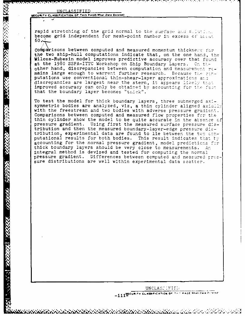
compa'isons between computed and measured momentum thickness forthe two ship-hull computations indicate that, on the one hand, theWilcox-Rubesin model improves predictive accuracy over that foundat the 1980 SSPA-ITTC Workshop on Ship Boundary Layers. On theother hand, discrepancies between computation and measurement re-mains large enough to warrent further research. Because the com-putations use conventional thin-shear-layer approximations anddiscrepancies are largest near the stern, it appears likely thatimproved accuracy can only be obtained by accounting for the factthat the boundary layer becomes "thick".
To test the model for thick boundary layers, three submerged axl-symmetric bodies are analyzed, viz, a thin cylinder aligned axiallywith the freestream and two bodies with adverse pressure gradient.Comparisons between computed and measured flow properties for thethin cylinder show the model to be quite accurate in the absence ofpressure gradient. Using first the measured surface pressure dis-tribution and then the measured boundary-layer-edge pressure dis-tribution, experimental data are found to lie between the two com-putational results for both bodies. This result indicates that byaccounting for the normal pressure gradient, model predictions for
* thick boundary layers should be very close to measurements. Anintegral method is devised and tested for computing the normalpressure gradient. Differences between computed and measured pres-sure distributions are well within experimental data scatter.
"-1
4
4
UNCLASSIFIED
_.iiiS cuRTy CLASStVICATION OF ' , PAGE(W'hen Date Entered)