environmentally sustainable livestock production
TRANSCRIPT

Environmentally Sustainable Livestock Production
Ilkka Leinonen
www.mdpi.com/journal/sustainability
Edited by
Printed Edition of the Special Issue Published in Sustainability

Environmentally Sustainable LivestockProduction


Environmentally Sustainable LivestockProduction
Special Issue Editor
Ilkka Leinonen
MDPI • Basel • Beijing • Wuhan • Barcelona • Belgrade

Special Issue Editor
Ilkka Leinonen
Scotland’s Rural College
UK
Editorial Office
MDPI
St. Alban-Anlage 66
4052 Basel, Switzerland
This is a reprint of articles from the Special Issue published online in the open access journal
Sustainability (ISSN 2071-1050) from 2018 to 2019 (available at: https://www.mdpi.com/journal/
sustainability/special issues/Environmentally Sustainable Livestock Production)
For citation purposes, cite each article independently as indicated on the article page online and as
indicated below:
LastName, A.A.; LastName, B.B.; LastName, C.C. Article Title. Journal Name Year, Article Number,
Page Range.
ISBN 978-3-03897-552-6 (Pbk)
ISBN 978-3-03897-553-3 (PDF)
c© 2019 by the authors. Articles in this book are Open Access and distributed under the Creative
Commons Attribution (CC BY) license, which allows users to download, copy and build upon
published articles, as long as the author and publisher are properly credited, which ensures maximum
dissemination and a wider impact of our publications.
The book as a whole is distributed by MDPI under the terms and conditions of the Creative Commons
license CC BY-NC-ND.

Contents
About the Special Issue Editor . . . . . . . . . . . . . . . . . . . . . . . . . . . . . . . . . . . . . . vii
Preface to ”Environmentally Sustainable Livestock Production” . . . . . . . . . . . . . . . . . . ix
Ilkka Leinonen
Achieving Environmentally Sustainable Livestock ProductionReprinted from: Sustainability 2019, 11, 246, doi:10.3390/su11010246 . . . . . . . . . . . . . . . . . 1
Nathan Pelletier, Maurice Doyon, Bruce Muirhead, Tina Widowski, Jodey Nurse-Gupta and
Michelle Hunniford
Sustainability in the Canadian Egg Industry—Learning from the Past, Navigating the Present,Planning for the FutureReprinted from: Sustainability 2018, 10, 3524, doi:10.3390/su10103524 . . . . . . . . . . . . . . . . 6
Nathan Pelletier
Social Sustainability Assessment of Canadian Egg Production Facilities: Methods, Analysis, andRecommendationsReprinted from: Sustainability 2018, 10, 1601, doi:10.3390/su10051601 . . . . . . . . . . . . . . . . 30
Tianyi Cai, Degang Yang, Xinhuan Zhang, Fuqiang Xia and Rongwei Wu
Study on the Vertical Linkage of Greenhouse Gas Emission Intensity Change of the AnimalHusbandry Sector between China and Its ProvincesReprinted from: Sustainability 2018, 10, 2492, doi:10.3390/su10072492 . . . . . . . . . . . . . . . . 47
Erasmus K.H.J. zu Ermgassen, Melquesedek Pereira de Alcantara, Andrew Balmford,
Luis Barioni, Francisco Beduschi Neto, Murilo M. F. Bettarello, Genivaldo de Brito,
Gabriel C. Carrero, Eduardo de A.S. Florence, Edenise Garcia, Eduardo Trevisan Goncalves,
Casio Trajano da Luz, Giovanni M. Mallman, Bernardo B.N. Strassburg, Judson F. Valentim
and Agnieszka Latawiec
Results from On-The-Ground Efforts to Promote Sustainable Cattle Ranching in the BrazilianAmazonReprinted from: Sustainability 2018, 10, 1301, doi:10.3390/su10041301 . . . . . . . . . . . . . . . . 65
Ana Beatriz Santos and Marcos Heil Costa
Do Large Slaughterhouses Promote Sustainable Intensification of Cattle Ranching in Amazoniaand the Cerrado?Reprinted from: Sustainability 2018, 10, 3266, doi:10.3390/su10093266 . . . . . . . . . . . . . . . . 91
Marıa I. Nieto, Olivia Barrantes, Liliana Privitello and Ramon Reine
Greenhouse Gas Emissions from Beef Grazing Systems in Semi-Arid Rangelands of CentralArgentinaReprinted from: Sustainability 2018, 10, 4228, doi:10.3390/su10114228 . . . . . . . . . . . . . . . . 119
Gwendolyn Rudolph, Stefan Hortenhuber, Davide Bochicchio, Gillian Butler,
Roland Brandhofer, Sabine Dippel, Jean Yves Dourmad, Sandra Edwards, Barbara Fruh,
Matthias Meier, Armelle Prunier, Christoph Winckler, Werner Zollitsch and Christine Leeb
Effect of Three Husbandry Systems on Environmental Impact of Organic PigsReprinted from: Sustainability 2018, 10, 3796, doi:10.3390/su10103796 . . . . . . . . . . . . . . . . 141
v

Ilkka Leinonen, Michael MacLeod and Julian Bell
Effects of Alternative Uses of Distillery By-Products on the Greenhouse Gas Emissions ofScottish Malt Whisky Production: A System Expansion ApproachReprinted from: Sustainability 2018, 10, 1473, doi:10.3390/su10051473 . . . . . . . . . . . . . . . . 161
Cristina Ullrich, Marion Langeheine, Ralph Brehm, Venja Taube, Diana Siebert and
Christian Visscher
Influence of Reduced Protein Content in Complete Diets with a Consistent Arginine–LysineRatio on Performance and Nitrogen Excretion in BroilersReprinted from: Sustainability 2018, 10, 3827, doi:10.3390/su10113827 . . . . . . . . . . . . . . . . 179
Henrik Saxe, Lorie Hamelin, Torben Hinrichsen and Henrik Wenzel
Production of Pig Feed under Future Atmospheric CO2 Concentrations: Changes in CropContent and Chemical Composition, Land Use, Environmental Impact, and Socio-EconomicConsequencesReprinted from: Sustainability 2018, 10, 3184, doi:10.3390/su10093184 . . . . . . . . . . . . . . . . 192
Katrin Gerlach, Alexander J. Schmithausen, Ansgar C. H. Sommer, Manfred Trimborn,
Wolfgang Buscher and Karl-Heinz Sudekum
Cattle Diets Strongly Affect Nitrous Oxide in the RumenReprinted from: Sustainability 2018, 10, 3679, doi:10.3390/su10103679 . . . . . . . . . . . . . . . . 210
Michael MacLeod, Vera Eory, William Wint, Alexandra Shaw, Pierre J. Gerber,
Giuliano Cecchi, Raffaele Mattioli, Alasdair Sykes and Timothy Robinson
Assessing the Greenhouse Gas Mitigation Effect of Removing Bovine Trypanosomiasis inEastern AfricaReprinted from: Sustainability 2018, 10, 1633, doi:10.3390/su10051633 . . . . . . . . . . . . . . . . 223
Ricarda Maria Schmithausen, Sophia Veronika Schulze-Geisthoevel, Celine Heinemann,
Gabriele Bierbaum, Martin Exner, Brigitte Petersen and Julia Steinhoff-Wagner
Reservoirs and Transmission Pathways of Resistant Indicator Bacteria in the Biotope Pig Stableand along the Food Chain: A Review from a One Health PerspectiveReprinted from: Sustainability 2018, 10, 3967, doi:10.3390/su10113967 . . . . . . . . . . . . . . . . 238
Marco Baldi, Maria Cristina Collivignarelli, Alessandro Abba and Ilaria Benigna
The Valorization of Ammonia in Manure Digestate by Means of Alternative Stripping ReactorsReprinted from: Sustainability 2018, 10, 3073, doi:10.3390/su10093073 . . . . . . . . . . . . . . . . 264
vi

About the Special Issue Editor
Ilkka Leinonen (Dr) works at the Department of Rural Economy, Environment and Society at
Scotland’s Rural College (SRUC), United Kingdom. He obtained his PhD from the University of
Joensuu (Finland) in 1997 and has since then carried out agricultural, ecological, and environmental
research, with a main interest in quantitative methodologies, especially process-based modelling
of ecosystem carbon, water, and nutrient dynamics. During recent years, he has mainly
focused on the environmental sustainability of agricultural production systems, using and further
developing methods of life cycle assessment (LCA) to quantify greenhouse gas emissions and other
environmental impacts of agriculture and to investigate mitigation strategies in the livestock sector,
for example, through changes in feeding, breeding, housing, and manure management. His other
expertise includes ecophysiological plant and animal modelling, physical energy balance modelling,
and methods for image analysis and remote sensing.
vii


Preface to ”Environmentally Sustainable Livestock
Production”
Livestock production is a major global source of greenhouse gas emissions and it is also
associated with other environmental issues, such as ammonia emissions and regional nutrient
imbalances. This Special Issue presents 14 scientific papers assessing measures that aim to improve
the environmental sustainability of livestock production and to mitigate its environmental impacts.
Globally, the most important livestock species (beef and dairy cattle, pigs, broiler chicken and
laying hens) are covered in the papers. The scope of the papers ranges from farm level mitigation
methods to national level system changes. In general, most of the papers identify the efficiency of
production as a key factor affecting the emissions arising from the livestock sector. In many studies,
holistic approaches, such as environmental life cycle assessment, are used to assess the possible
improvements in emission intensity, and the required links to other dimensions of sustainability,
for example, using the methodology of social life cycle assessment, are also demonstrated in this
Special Issue.
Ilkka Leinonen
Special Issue Editor
ix


sustainability
Editorial
Achieving Environmentally SustainableLivestock Production
Ilkka Leinonen
Department of Rural Economy, Environment and Society, Scotland’s Rural College (SRUC), Peter WilsonBuilding, Kings Buildings, West Mains Road, Edinburgh EH9 3JG, UK; [email protected];Tel.: +44-131-5354044
Received: 2 January 2019; Accepted: 4 January 2019; Published: 7 January 2019
Livestock production is a major global source of greenhouse gas emissions [1] and high density oflivestock in certain areas can also create local environmental issues such as harmful levels of ammoniaemissions and regional nutrient imbalances [2,3]. However, future improvements in the global livestocksector can also be seen as a potential opportunity for delivering a significant share of the necessarymitigation of global warming and other environmental problems [1]. In fact, it has been demonstratedthat significant reductions in various environmental impacts and especially in the emissions intensities(i.e., the amount of emissions per unit of product) have been already achieved in livestock productionduring the past decades, for example through breeding, optimized feeding, improved health status ofanimals, and improved manure management [4–6].
This Special Issue presents results from studies on different measures aiming to improve theenvironmental sustainability of livestock production and to mitigate environmental impacts, includingemissions of greenhouse gases (carbon dioxide, methane, and nitrous oxide), nitrogen and phosphorusexcretion, ammonia emissions, land use and use of energy and other resources. Globally the mostimportant livestock species (beef and dairy cattle, pigs, broiler chicken and laying hens) are coveredin the papers published here. The mitigation methods assessed in the papers include general systemchanges (together with novel approaches to comparison of alternative production systems), changes infeeding, improvement of animal health, and new technologies of manure management.
The scope of the papers included in this Special Issue range from farm level mitigation methods tonational level system changes. One of the national-level articles, written by Pelletier et al. [7], presentsan overview of the sustainability of the Canadian egg production industry. The authors providean interdisciplinary perspective to this industry, considering its past, present, and potential futures.Their analysis covers environmental, institutional, and socio-economic sustainability with a specialemphasis on animal welfare. The analysis identifies major challenges for sustainable egg industry,including shifting consumer and other stakeholder preferences and expectations, and conflicts betweenthe expectations and scientific evidence. A thorough discussion is provided on possible strategies toresolve these issues.
The methodology of Life Cycle Assessment (LCA) is becoming a standard in evaluating theenvironmental sustainability of livestock systems, but LCA also has applications in the areas ofsocial (S-LCA) and economic (life cycle costing) sustainability assessment. In contrast to relativelywell established methods of environmental Life Cycle Assessment, the methods of S-LCA are stillunder development. In his second paper in this Special Issue, Nathan Pelletier [8] develops a suiteof context-appropriate indicators and metrics to characterize the social risks and benefits specificto activities at Canadian egg production facilities and then applies those indicators to perform adetailed assessment of the “gate-to-gate” social risks and benefits of Canadian egg production facilities.The analysis presented here provides a starting point for expanding the methodology to cover thewhole production chain and thus enable a full social life cycle assessment.
Sustainability 2019, 11, 246; doi:10.3390/su11010246 www.mdpi.com/journal/sustainability1

Sustainability 2019, 11, 246
In their paper, Cai et al. [9] carry out a national level study on a reduction of the emission intensities(per unit of the monetary value of output) of non-CO2 greenhouse gases arising from the livestocksector in China, through an analysis of the contribution of each province to the overall nationalemissions. They especially concentrate on the role of three “driving factors,” i.e., environmentalefficiency, productive efficiency and economic share, in determining the national greenhouse gasemission intensity. Their findings suggest that the productive efficiency (i.e., the input of productionfactors per unit of output value) is the main contributor to the changes in the emission intensities,and improvement in this factor has resulted in a considerable reduction of livestock sector emissionintensity at the national level during the period of 1997–2016.
The effect of system changes on the productivity of cattle production in the Amazon biome wasevaluated by zu Ermgassen et al. [10]. The key question in their study is how to handle the increasingagricultural production in Brazil (e.g., currently the World’s second largest cattle herd) and at the sametime protect remaining natural vegetation. The authors found that currently the cattle productivity inthe Amazon biome is very low, and intensification of the cattle production systems would be the keyfactor in achieving higher environmental sustainability. In their paper, they present results from sixinitiatives in the Brazilian Amazon, which have successfully improved the productivity in beef anddairy systems.
Brazilian livestock production is also considered in the paper by Santos and Costa [11]. They testedthe hypothesis according to which large slaughterhouses are potential leverage points for promotingsustainable intensification in the beef supply chain in Amazonia and the Cerrado, due to theirinteractions with ranchers, their location at the agricultural frontier, and their ability to control accessto the market. The authors’ conclusion was that although cattle-ranching intensification (with positiveeffect on environmental indicators) has occurred in the Cerrado, this development is independent ofthe presence of large slaughterhouses. Instead, the authors suggest that conservation measures such asa strong monitoring systems and more restrictive environmental policies would be the key promotesof environmental sustainability, especially at the Amazonia region.
In their article, Nieto et al. [12] assess the on-farm greenhouse gas emissions from beef productionin semi-arid rangelands in Argentina and apply statistical analyses to identify the relationshipbetween emissions and current farm management practices. Their results highlight the importance ofefficient production in achieving environmental sustainability of livestock production. Their findingsindicate that the emissions per product were low on farms that had improved livestock caremanagement, applied rotational grazing, and had access to technical advice. The authors suggest that“implementation of realistic, relatively easy-to-adopt farming management practices has considerablepotential for mitigating the GHG emissions in the semi-arid rangelands of central Argentina.”
Livestock production in Europe has been considered to be highly intensive, and thus relativelyefficient. However, many low-intensity systems exist as well, especially in organic production. In thestudy by Rudolph et al. [13] a system comparison using environmental LCA was carried for threeEuropean organic pig production systems, namely indoor, partly outdoor, and outdoor. The authorsfound a great between-farm variation in three environmental indicators: global warming, acidificationand eutrophication potentials. The differences between the farms were mainly affected by feedproduction and to some extent also by housing. There were no between-system differences in globalwarming potential, but acidification potential was highest in the indoor system (as a result of ammoniaemissions) and the eutrophication potential highest in the outdoor system (as a result of nutrientleaching). The authors conclude that the occurrence of organic farms with low environmental impactsindicates that it is possible to manage organic pig production in an environmentally friendly way.
Using agricultural by-products (that are not suitable for human consumption) as part of livestockfeed has been considered to be one method to improve the environmental sustainability of livestockproduction. In their study, Leinonen et al. [14] assess the environmental consequences of using distilleryby-products as a protein source for beef cattle in Scotland. Their study highlights the complexityof livestock feed production chains. This was demonstrated by the alternative uses of agricultural
2

Sustainability 2019, 11, 246
by-products (in this case either as a livestock feed or as a source of renewable energy), and theenvironmental impacts arising from those options were analyzed through the system expansion-basedLCA approach.
Another option to reduce the environmental impacts through livestock feeding is to apply resourceefficient feed formulation. Ullrich et al. [15] evaluated the potential of reducing the crude protein levelof the broiler diet by using supplementation of single amino acids to achieve an optimum amino acidbalance of the feed. Their experimental results confirm some earlier modelling studies [16] accordingto which a balanced diet with lowered crude protein concentration can reduce the amount of nitrogenexcreted, which has multiple environmental benefits. It is also demonstrated that such an improvementcan be achieved without compromising animal performance.
The link between livestock feeding and climate change is not only a one direction process. The feedformulation in the future may also be affected by changes in the availability and quality of certainfeed ingredients, and such changes can be induced by global warming and increased atmosphericCO2 concentration. Saxe et al. [17] applied a consequential life cycle assessment to quantify theenvironmental impacts and socio-economic effects that altered crop yields and chemical compositionof the crops at elevated CO2 levels in the future can have on pig feed formulation. They predict thatthe elevated CO2 reduces the land use demand for pig feed production, but at the same time increasesthe demand for protein crops (soya), due to reduced protein concentration of feed crops. This willhave considerable environmental and economic consequences.
In cattle production, methane from enteric fermentation and manure management is generallyconsidered to be the most significant greenhouse gas. However, nitrous oxide emissions related toruminant feeding have also their own role in the total emissions from this livestock sector. In theirarticle, Gerlach et al. [18] present a new method for determining the concentrations of CO2, CH4, andN2O in the ruminal gas phase of steers after ingestion of different forage types. Depending on the diet,high concentration of N2O were found in the rumen, indicating that that fermented forages rich innitrogen can be a significant source of greenhouse gases.
Improving the health status of animals is one option to maintain high production efficiencyof livestock and in this way keep the emission intensity at the minimal level. In their paper,MacLeod et al. [19] apply the FAO livestock model GLEAM to quantify the greenhouse gas emissionsfrom East African cattle production systems and the effects of an endemic disease trypanosomiasis onthe emissions. The authors found that removing that disease could lead to a reduction in the emissionsintensity per unit of protein produced, as a result of increases in milk yields and higher cow fertilityrates. Another major issue related to animal health is antibiotic resistance, and this has also links to theenvironmental impacts of livestock production. In their comprehensive review, Schmithausen et al. [20]highlight knowledge gaps and various factors that contribute to the transmission of antibiotic-resistantbacteria between animals, humans, and the environment in pig production, following a holistic “OneHealth” approach.
Although most papers in this special issue focus on livestock husbandry and its effect on animalperformance when considering possible methods for reducing the environmental impacts of livestocksystem (and their potential effects on human health), different manure management options canpotentially also control such impacts. Reduction of ammonia emission through improved manuremanagement has direct consequences on human and animal health, and it also affects numerousenvironmental issues such as eutrophication, acidification, and global warming. In this Special Issue,novel technologies of manure management are considered in the paper by Baldi et al. [21], who showresults of a comparison of ammonia stripping methods aiming to reduce the emissions arising fromdigestate derived from anaerobic digestion of livestock manure and corn silage.
In summary, this Special Issue demonstrates a range of opportunities that would help to reducethe environmental impacts of global livestock production. Most of the papers identify the efficiencyof the production as a key factor to affect the emission intensity of the livestock products. To assessthe possible improvements in efficiency, holistic approaches such as Live Cycle Assessment would
3

Sustainability 2019, 11, 246
be necessarily needed, and further methodological development in this area is still required [22].This would be especially a challenge when linking together the three pillars of sustainability(environmental, social, and economic) in sustainability assessments of livestock production.
Funding: This research was partly funded by the Scottish Government Rural Affairs and the EnvironmentPortfolio Strategic Research Programme 2016-2021, WP 1.4 ‘Integrated and Sustainable Management of NaturalAssets’ and 2.4 ‘Rural Industries’.
Conflicts of Interest: The author declares no conflict of interest.
References
1. Gerber, P.J.; Steinfeld, H.; Henderson, B.; Mottet, A.; Opio, C.; Dijkman, J.; Falcucci, A.; Tempio, G. TacklingClimate Change through Livestock. A Global Assessment of Emissions and Mitigation Opportunities; Food andAgriculture Organization of the United Nations (FAO): Rome, Italy, 2013; ISBN 978-92-5-107921-8.
2. Vitousek, P.M.; Naylor, R.; Crews, T.; David, M.B.; Drinkwater, L.E.; Holland, E.; Johnes, P.J.; Katzenberger, J.;Martinelli, L.A.; Matson, P.A.; et al. Nutrient imbalances in agricultural development. Science 2009, 324,1519–1520. [CrossRef]
3. Leinonen, I.; Eory, V.; MacLeod, M. Applying a process-based livestock model to predict spatial variation inagricultural nutrient flows in Scotland. J. Clean. Prod. 2018, 209, 180–189. [CrossRef]
4. Pelletier, N.; Ibarburu, M.; Xin, H. Comparison of the environmental footprint of the egg industry in theUnited States in 1960 and 2010. Poult. Sci. 2014, 93, 241–255. [CrossRef] [PubMed]
5. Tallentire, C.W.; Leinonen, I.; Kyriazakis, I. Breeding for efficiency in the broiler chicken. A review.Agron. Sustain. Dev. 2016, 36, 66. [CrossRef]
6. Tallentire, C.W.; Leinonen, I.; Kyriazakis, I. Artificial selection for improved energy efficiency is reaching itslimits in broiler chickens. Sci. Rep. 2018, 8, 116. [CrossRef] [PubMed]
7. Pelletier, N.; Doyon, M.; Muirhead, B.; Widowski, T.; Nurse-Gupta, J.; Hunniford, M. Sustainability inthe Canadian Egg Industry—Learning from the Past, Navigating the Present, Planning for the Future.Sustainability 2018, 10, 3524. [CrossRef]
8. Pelletier, N. Social Sustainability Assessment of Canadian Egg Production Facilities: Methods, Analysis, andRecommendations. Sustainability 2018, 10, 1601. [CrossRef]
9. Cai, T.; Yang, D.; Zhang, X.; Xia, F.; Wu, R. Study on the Vertical Linkage of Greenhouse Gas EmissionIntensity Change of the Animal Husbandry Sector between China and Its Provinces. Sustainability 2018, 10,2492. [CrossRef]
10. Zu Ermgassen, E.; Alcântara, M.; Balmford, A.; Barioni, L.; Neto, F.; Bettarello, M.; Brito, G.; Carrero, G.;Florence, E.; Garcia, E.; et al. Results from On-The-Ground Efforts to Promote Sustainable Cattle Ranching inthe Brazilian Amazon. Sustainability 2018, 10, 1301. [CrossRef]
11. Santos, A.; Costa, M. Do Large Slaughterhouses Promote Sustainable Intensification of Cattle Ranching inAmazonia and the Cerrado? Sustainability 2018, 10, 3266. [CrossRef]
12. Nieto, M.; Barrantes, O.; Privitello, L.; Reiné, R. Greenhouse Gas Emissions from Beef Grazing Systems inSemi-Arid Rangelands of Central Argentina. Sustainability 2018, 10, 4228. [CrossRef]
13. Rudolph, G.; Hörtenhuber, S.; Bochicchio, D.; Butler, G.; Brandhofer, R.; Dippel, S.; Dourmad, J.; Edwards, S.;Früh, B.; Meier, M.; et al. Effect of Three Husbandry Systems on Environmental Impact of Organic Pigs.Sustainability 2018, 10, 3796. [CrossRef]
14. Leinonen, I.; MacLeod, M.; Bell, J. Effects of Alternative Uses of Distillery By-Products on the GreenhouseGas Emissions of Scottish Malt Whisky Production: A System Expansion Approach. Sustainability 2018, 10,1473. [CrossRef]
15. Ullrich, C.; Langeheine, M.; Brehm, R.; Taube, V.; Siebert, D.; Visscher, C. Influence of Reduced ProteinContent in Complete Diets with a Consistent Arginine–Lysine Ratio on Performance and Nitrogen Excretionin Broilers. Sustainability 2018, 10, 3827. [CrossRef]
16. Leinonen, I.; Williams, A.G. Effects of dietary protease on nitrogen emissions from broiler production: Aholistic comparison using Life Cycle Assessment. J. Sci. Food Agric. 2015, 95, 3041–3046. [CrossRef]
4

Sustainability 2019, 11, 246
17. Saxe, H.; Hamelin, L.; Hinrichsen, T.; Wenzel, H. Production of Pig Feed under Future Atmospheric CO2Concentrations: Changes in Crop Content and Chemical Composition, Land Use, Environmental Impact,and Socio-Economic Consequences. Sustainability 2018, 10, 3184. [CrossRef]
18. Gerlach, K.; Schmithausen, A.; Sommer, A.; Trimborn, M.; Büscher, W.; Südekum, K. Cattle Diets StronglyAffect Nitrous Oxide in the Rumen. Sustainability 2018, 10, 3679. [CrossRef]
19. MacLeod, M.; Eory, V.; Wint, W.; Shaw, A.; Gerber, P.; Cecchi, G.; Mattioli, R.; Sykes, A.; Robinson, T.Assessing the Greenhouse Gas Mitigation Effect of Removing Bovine Trypanosomiasis in Eastern Africa.Sustainability 2018, 10, 1633. [CrossRef]
20. Schmithausen, R.; Schulze-Geisthoevel, S.; Heinemann, C.; Bierbaum, G.; Exner, M.; Petersen, B.;Steinhoff-Wagner, J. Reservoirs and Transmission Pathways of Resistant Indicator Bacteria in the Biotope PigStable and along the Food Chain: A Review from a One Health Perspective. Sustainability 2018, 10, 3967.[CrossRef]
21. Baldi, M.; Collivignarelli, M.; Abbà, A.; Benigna, I. The Valorization of Ammonia in Manure Digestate byMeans of Alternative Stripping Reactors. Sustainability 2018, 10, 3073. [CrossRef]
22. Mackenzie, S.G.; Leinonen, I.; Kyriazakis, I. The need for co-product allocation in the Life Cycle Assessmentof agricultural systems—Is “biophysical” allocation progress? Int. J. Life Cycle Assess. 2017, 22, 128–137.[CrossRef]
© 2019 by the author. Licensee MDPI, Basel, Switzerland. This article is an open accessarticle distributed under the terms and conditions of the Creative Commons Attribution(CC BY) license (http://creativecommons.org/licenses/by/4.0/).
5

sustainability
Article
Sustainability in the Canadian EggIndustry—Learning from the Past,Navigating the Present, Planning for the Future
Nathan Pelletier 1,* , Maurice Doyon 2, Bruce Muirhead 3, Tina Widowski 4,
Jodey Nurse-Gupta 5 and Michelle Hunniford 6
1 340 Charles Fipke Centre for Innovative Research, 3247 University Way, University of British Columbia,Kelowna, BC V1V1V7, Canada
2 Department of Agricultural Economics and Consumer Science, Laval University, Quebec City, QC G1V 0A6,Canada; [email protected]
3 Research Oversight and Analysis and Department of History, University of Waterloo, Waterloo,ON N2L 3G1, Canada; [email protected]
4 Department of Animal Biosciences, University of Guelph, Guelph, ON N1G2W1, Canada;[email protected]
5 Department of History, University of Waterloo, Waterloo, ON N2L 3G1, Canada; [email protected] Burnbrae Farms Ltd., Lyn, ON K0E1M0, Canada; [email protected]* Correspondence: [email protected]; Tel.: +1-250-807-8245
Received: 30 August 2018; Accepted: 27 September 2018; Published: 30 September 2018
Abstract: Like other livestock sectors, the Canadian egg industry has evolved substantially overtime and will likely experience similarly significant change looking forward, with many of thesechanges determining the sustainability implications of and for the industry. Influencing factorsinclude: technological and management changes at farm level and along the value chain resultingin greater production efficiencies and improved life cycle resource efficiency and environmentalperformance; a changing policy/regulatory environment; and shifts in societal expectations andassociated market dynamics, including increased attention to animal welfare outcomes—especiallyin regard to changes in housing systems for laying hens. In the face of this change, effectivedecision-making is needed to ensure the sustainability of the Canadian egg industry. Attentionboth to lessons from the past and to the emerging challenges that will shape its future is requiredand multi- and interdisciplinary perspectives are needed to understand synergies and potentialtrade-offs between alternative courses of action across multiple aspects of sustainability. Here, weconsider the past, present and potential futures for this industry through the lenses of environmental,institutional (i.e., regulatory), and socio-economic sustainability, with an emphasis on animal welfareas an important emergent social consideration. Our analysis identifies preferred pathways, potentialpitfalls, and outstanding cross-disciplinary research questions.
Keywords: Canada; eggs; sustainability; animal welfare; economics; supply management
1. Introduction
Food systems are at the center of human well-being. In addition to satisfying a basic human need(i.e., regular access to food in sufficient quantity and of sufficient quality), food is also often a centralcontributor to our economies and cultures, and often even to our individual identities. However,activities in the agri-food system are also at the center of many of our most pressing sustainabilitychallenges. The production of food—in particular, in the livestock sector—contributes a large fraction ofcurrent anthropogenic resource demands and environmental pressures [1–3]. For this reason, livestockindustries are naturally the focus of a growing body of sustainability research and managementinitiatives [4].
Sustainability 2018, 10, 3524; doi:10.3390/su10103524 www.mdpi.com/journal/sustainability6

Sustainability 2018, 10, 3524
Taken together with projected increases in food production globally and a trend towards dietshigher in livestock products, this has spurred considerable interest in the concept and practice of“sustainable intensification” in the livestock sector [4]. According to Pretty et al. [5], sustainableintensification is defined as “producing more output from the same area of land while reducingnegative environmental impacts and at the same time increasing contributions to natural capital andthe flow of environmental services.” Clearly, however, sustainable intensification efforts may also havepotential benefits and trade-offs across socio-economic, institutional, and other aspects of sustainabilitythat must be carefully considered.
Life cycle thinking (LCT) has emerged as a core concept in sustainability science [6]. LCT refers toadopting a systems-level perspective on industrial activities. This perspective enables us to understandhow different kinds of potential sustainability benefits and impacts are distributed along agri-foodsupply chains, as well as trade-offs that may occur with respect to different valued outcomes whenparticular changes are implemented. Environmental life cycle assessment (e-LCA) is a commonlyused tool, based on LCT, for studying and managing the resource/environmental dimensions of foodsupply chains [4]. In recent years, a rich body of research has applied this tool to evaluate a variety oflivestock production systems and technologies in different contexts, and as a basis for understandingthe respective merits of potential sustainable intensification technologies (for a review of 173 recentpapers, see McClelland et al. [7]).
While such research is clearly of considerable value, it is by itself insufficient to supportsustainability decision-making for the livestock sector since it considers only a subset of importantsustainability criteria that inform our decisions [8]. In reality, the varied forces that influence how weproduce and consume livestock products along with the associated benefits and impacts are complex,often interacting, and variable over time. They include changes in technology and managementpractices, evolving societal expectations and consumer preferences, and the regulatory context inwhich specific industries operate. Efforts to understand current sustainability challenges in thelivestock sector and to identify preferred paths forward can benefit from interdisciplinary approachesthat evaluate these forces with respect to historical trends, current conditions, and possible futures.
Egg Farmers of Canada, the industry body governing the production and marketing of eggs withinthe supply-managed Canadian egg industry, provides research monies to support four Research Chairsat Canadian universities. These Research Chairs respectively undertake independent research in thefields of economics (Doyon), public policy (Muirhead), animal welfare (Widowski), and sustainability(Pelletier) of broad or direct relevance to the egg industry. The current analysis brings together theexpertise, research, and perspectives of each of these Chairs to present an integrated study of thepast, present and possible futures for this industry. Specifically, the purpose of the analysis is toidentify: (1) the key factors that have shaped the modern Canadian egg industry; (2) the issuesand opportunities it currently faces; and (3) potential synergies and trade-offs across the multipledimensions of sustainability that should be considered on an interdisciplinary basis in choosing amongviable paths looking forward.
2. Methods
The analysis is presented in three sections. The first section provides a historical perspective,describing the emergence and evolution of the Canadian egg industry over the past century until thepresent. It is organized into subsections respectively addressing: key technological and managementchanges, including their influence on the efficiency and environmental sustainability impacts ofegg production; the development and implications of the supply management system that governsthe industry; the factors that have influenced the economics of egg production, including changingconsumer preferences and social expectations; and, as an important aspect of the latter, the emergenceof animal welfare as both a societal concern and field of study/application for the egg industry.
The second section, also organized into four subsections, describes challenges that the industrycurrently faces in each of these domains that may undermine its sustainability, as well as potential
7

Sustainability 2018, 10, 3524
solutions. Possible trade-offs across sustainability domains that such solutions may imply are identified.On this basis, the final section summarizes some of the key areas for interdisciplinary research andcollaboration that are necessary to support choosing among alternative courses of action to enable asustainable egg industry in Canada into the future.
3. Discussion
3.1. Canadian Egg Industry Retrospective (Circa 1920 to Present)
3.1.1. Technology, Management, and Resource Efficiency
Although a small number of specialized, commercial egg farms in Canada existed in the earlypart of the 20th century, egg production was generally one among a series of activities undertaken onthe mixed-farming operations that were characteristic of Canadian agriculture at that time. Beginningin the 1920s, however, the egg industry entered a period of significant and sustained industrialization.Two major developments that were particularly important to the specialization and intensificationof egg production were the adoption of cage systems for housing laying hens and improved geneticselection for egg production and feed conversion efficiency.
From 1923–1924, D.C. Kennard performed the first experiments keeping laying hens inconfinement at the Ohio Agricultural Research Station, using livability and production as the mainmeasures of success [9]. However, cage systems were not immediately adopted for commercial use.This was because indoor confinement for longer periods of time was only possible once the completeration, which was developed in 1924, was made available on the wider market in 1929 and the RuralElectrification Act of 1936 in the US enabled barns to be lit artificially. The ability to keep laying hensindoors revolutionized the egg industry [10,11]. Whereas eggs were previously a seasonal (spring)food in temperate climates, they could now be produced continuously year-round [12].
According to Lee, 1938 marked the year when farmers had “satisfactorily solved the manyproblems of management which were responsible for the failure of earlier battery plants (so calledbecause of the methodical (militaristic) nature of organizing the cages in stacked groups orbatteries)” [10]. The need for steel during World War II, however, meant that the production ofcages was halted (except for a small number of chick batteries) until after the war when the batterycage boom started on the Pacific coast of the US and in the UK [10].
Individual cages were initially used because they eliminated issues with cannibalism and allowedfor the practice of “positive culling,” or removing birds from the flock that are “laying at a slowunprofitable rate or [have] quit laying altogether” [13]. However, due to the cost advantages ofhousing multiple birds in the same cage, the battery cage was adapted to house small groups ofhens [14]. Beginning in the 1960s egg production in Canada transitioned from “free-run” (i.e., indoornon-cage) to cage-based production.
Genetic selection of laying hens for egg production and feed use efficiency in cage systems alsobegan in earnest following World War II. Canadian Donald Shaver built a global breeding organizationfor layer and broiler strains [15]. The availability of electricity-powered incubators and the relativelyshort incubation cycle for eggs facilitated rapid progress in selection for production efficiency [16].At the same time, development of improved management practices for disease prevention such asbiosecurity protocols, along with the advent of poultry vaccines, served to improve bird health andreduce losses due to mortality [17,18]. Over time, advancements in housing technology includingartificial ventilation systems and climate control, automated feeding, egg collection and manureremoval were implemented, thereby reducing labor and allowing for thousands or tens of thousandsof birds to be housed in a single barn.
In combination, these technology and management changes have enabled considerableimprovements in resource efficiency and the reduction of environmental impacts associated withproducing eggs in Canada. For example, annual rate of lay among Canadian laying hens has increasedfrom less than 100 eggs per year in the early 20th century to over 300 at present [19]. Between 1962
8

Sustainability 2018, 10, 3524
and 2012, an interval of 50 years, rate of lay increased by more than 50%. This same 50-year intervalwas also marked by declining mortality rates (falling from roughly 13% in the early 1960s to 3.2% atpresent for pullets and laying hens combined), and by much improved feed conversion efficiencies.With respect to the latter, producing 1 kg of eggs in 1962 required over 3 kg of feed compared to thecurrent average of 2 kg on contemporary egg farms [20].
Efficiency changes have been equally pronounced along the supply chains that ultimatelysupport Canadian egg production. Among these, the most influential in terms of life cycle resourceuse/emissions-related sustainability impacts have been: (a) a 50% reduction in the energy intensity ofammonia production for nitrogen fertilizers (one of the most energy and emissions intensive aspectsof modern agriculture); (b) improved yield-to-fertilizer and energy input ratios for the production ofagricultural feed inputs (for example, corn yields in the province of Ontario increased 96% over thisinterval while nitrogen inputs per ton of crop declined 44%); and (c) improved efficiencies in freighttransport, which connect activities all along the Canadian egg supply chain [20].
As a result, of these changes, the overall environmental footprint (i.e., including all supply chainactivities) of producing eggs in Canada has, on average, declined 61%, 68%, and 72% for acidifying,eutrophying, and greenhouse gas (GHG) emissions while energy, land and water use decreasedby 41%, 81% and 69% respectively per unit production. Moreover, despite that egg productionvolumes roughly doubled in Canada since the early 1960s, the absolute resource and environmentalimpacts for the industry as a whole were estimated to be 41%, 51% and 57% lower for acidifying,eutrophying, and greenhouse gas emissions, respectively. Supply chain energy, land and water useare 10%, 71% and 53% lower in aggregate [20]. These changes reflect a combination of farm-levelefficiency gains (15–40%, depending on impact category) associated with improved managementpractices, superior bird genetics, and vaccine developments; changes in feed composition (29–60%);and changing efficiencies in activities along the supply chains that ultimately support egg production(0–56%) [20].
Life cycle assessment research has hence enabled a nuanced understanding of both the magnitudeand distribution of a variety of environmental sustainability impacts along the contemporary Canadianegg supply chain, the relative importance of specific inputs to and activities associated with eggproduction as sources of these impacts, and the comparative impacts of egg production in alternativehousing systems [21]. A relatively small number of variables explain the characteristic sources anddistribution of life cycle resource use and emissions for eggs and egg product supply chains in Canada.Among these, feed composition and feed conversion efficiency in pullet and (in particular) layerfacilities emerge as the strongest explanatory variables. Manure management is the second criticaldeterminant of life cycle resource efficiency and emissions. Manure-related emissions are influencedby several factors, including feed composition (i.e., N and P content of feed inputs), feed conversionefficiencies, and manure handling strategies. Although more strongly influenced by supply chainfeed inputs, direct water and energy use in facilities also make non-trivial contributions to the overallwater and energy resource requirements for egg production. The contributions of egg processing andpackaging, as well as egg breaking and further processing to overall supply chain resource use andemissions for eggs and egg products are relatively small [21]. These insights are largely consistent withsimilar research of intensive egg production in other countries (for example, [18,22–27]).
Pelletier [21] reported resource efficiencies and life cycle environmental performance by housingsystem type for the Canadian egg industry in 2012. Among the five housing technologies considered(i.e., conventional cages, enriched colony cages (which provide all of the equipment found inconventional cages with the addition of equipment that is intended to allow hens to express some oftheir behavioral priorities), free-run, free-range, and organic), both the life cycle inventory and impactassessment results suggested fairly similar levels of performance between systems for most variables.Feed conversion efficiencies were slightly higher in cage-based production, and mortality rates weresubstantially lower compared to non-cage systems. Of note was the higher variability in performancelevels observed between reporting facilities for non-cage production systems, likely reflecting the
9

Sustainability 2018, 10, 3524
substantial research and development investments and management experience gained for cage-basedproduction over time relative to the emerging cage-free sector. Only for organic production were lifecycle resource use and emissions significantly different from the other housing systems [21]. Here,the lower observed resource use and emissions intensity of organic eggs was attributable to thelower impacts of feed production rather than differences in farm-level efficiencies, where mortalityrates were highest among the housing systems considered. At present, over 80% of laying hens inCanada are kept in conventional cages, and the remainder in either enriched cages, free-run barns, orfree-range systems.
3.1.2. Shifting Regulatory Conditions for the Production and Marketing of Eggs
The intensification of the egg industry from the 1920s onward meant that increasing numbers ofeggs were finding their way onto the market. While the consumption of eggs rose steadily over time,the growth in egg production often outstripped demand, leading to overproduction and hardship foregg farmers [28,29]. Critically, farmers only received prices that allowed a fair return for short periodsof time after low prices had pushed out the most vulnerable producers. While a shortage of productbriefly forced prices up, the cycle would start over as farmers re-entered the business or ramped upproduction and again prices would plummet due to an oversupply of eggs. This was a perennialproblem and the Canadian Minister of Agriculture in 1959, Douglas Harkness, noted that “The onlylong-term solution to the current problem is a decrease in egg production to the point where there is amore realistic balance between supply and domestic requirements” [30].
An additional complication was cheap egg imports from the United States. This meant Canadianfarmers often had to accept egg prices that not only reflected tough domestic competition, but alsoa cheaper international price. The US, with its more robust economies of scale, undercut Canadianprices. Furthermore, provinces with surplus production would seek markets outside their borders,often undercutting prices and causing local producers’ incomes to drop [31].
The new realities of the price-cost squeeze borne by agricultural producers and trends towardsmore specialized, capitalized, and vertically integrated operations caused significant concern amongfamily farmers who saw producer prices drop and their earnings decrease despite ever more costly farminvestments. While some industry experts believed that the movement towards vertical integrationwas inevitable and that only a few of the largest Canadian egg producers would survive, othersargued that egg producers needed to create a system that would permit them to succeed without thecorporatization of the family farm [32,33].
The continued instability of egg prices galvanized discussions about the need for farmers toorganize and institute measures that would secure fair returns. Foremost among these discussionswere proposals to create provincial marketing boards to regulate the production and sale of eggs on aquota system basis. Critics of the idea of marketing boards cited infringements on their freedom to actindependently. Some egg farmers also recognized that provincial production quotas would only workif a national production plan were instituted that addressed the issue of egg imports from the US [34].
In July 1971, provincial representatives reached an agreement in principle whereby productionwould be controlled by marketing boards in each province and the national market would be sharedbased on average production figures calculated from 1968 to 1970. This led to the passage of the FarmProducts Marketing Agencies Act in January 1972, which allowed for the creation of the CanadianEgg Marketing Agency (CEMA) later that year. The system of “supply management” had come to theCanadian egg industry [35].
Despite some initial growing pains, by 1976 CEMA had turned the corner, becoming solvent andrevising and consolidating the comprehensive egg marketing plan, which meant uniform pricing,quota planning, and overproduction penalties introduced in all provinces. The processes were cominginto place that allowed for the successful operation of a national supply management system thatpromoted its social and economic sustainability. The system of supply management helped end marketchaos and enabled farmers to earn a living wage and offer consumers a fair price, while demonstrating
10
Sustainability 2018, 10, 3524
a commitment to improved egg farming practices. At present, CEMA, renamed Egg Farmers of Canadain 2008, oversees the quota-based production and marketing of eggs from over 1000 farms distributedacross all ten Canadian provinces and one territory.
3.1.3. Shifting Social Preferences and Socio-Economic Conditions
Supply Management
Over the years, the economics of the egg industry has been driven by improvements in technology,genetics, feeds, and management; resulting in productivity gains in rate of lay, in feed conversion andin lower mortality rates. Supply management, which shaped the marketing of eggs in Canada since1971, has been similarly important for the economics of egg production, largely through the preventionof egg surpluses—a primary rationale for its implementation. Production controls were intended toprevent the boom/bust cycle of commodities production. Whereas the huge swings so characteristicof commodity sales played havoc with planning and investment [36], supply management providedincome stability for farmers and, for consumers, predictability in meal costing and planning [37].
Price fluctuations were also perceived to favor processors and supermarkets, who drove downthe prices paid to farmers. Indeed, many farmers believed that they were being exploited by severalruthless buyers who were only interested in making money [38]. In July 1971, for example, a dozeneggs cost 17 cents retail in Toronto, while the cost of production was about 31 cents. Prices were,in the words of a Canadian Egg Producers Council document provided to the minister of agriculture,“disastrously low . . . extending from 1970, through 1971 and the first half of 1972” [39].
As the document went on to note, “Not only this but the public interest is badly served by theeconomic waste and inefficiency that is an inevitable consequence of severe cyclical instability, andby the instability of consumer prices—sometimes extremely (and to the producer disastrously) low,but at others unnecessarily high as production inevitably falls to inadequate levels under the pressureof persistent losses.” With the passage of Bill C-176, the Farm Products Marketing Agencies Act on 31December 1971, the way was clear to establish a national system of egg production, based on provincialorganization, that soon stabilized production, farmer incomes, and consumer prices. Significantimprovement in farm income for egg farmers subsequently allowed them to invest in technology, aswell as to respond to changes in consumer demand, such as for specialty eggs [40].
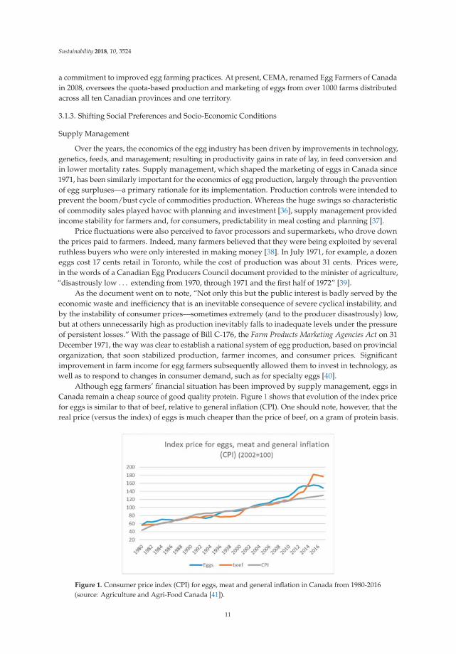
Although egg farmers’ financial situation has been improved by supply management, eggs inCanada remain a cheap source of good quality protein. Figure 1 shows that evolution of the index pricefor eggs is similar to that of beef, relative to general inflation (CPI). One should note, however, that thereal price (versus the index) of eggs is much cheaper than the price of beef, on a gram of protein basis.
Figure 1. Consumer price index (CPI) for eggs, meat and general inflation in Canada from 1980-2016(source: Agriculture and Agri-Food Canada [41]).
11

Sustainability 2018, 10, 3524
Shifting Consumer Preferences
The third major variable impacting the economics of egg production has been shifting consumerpreferences. For instance, in 1980, Canadians were consuming roughly 22 dozen eggs a year. However,due to cholesterol concerns in the 80s and 90s, per capita consumption reached a low of 14.5 dozen in1995, as illustrated in Figure 2. New research and a better comprehension of the various types of fatshas rehabilitated egg consumption, which has been steadily increasing to the current annual rate ofmore than 20 dozen eggs per capita. Thus, Canadian egg farmers have seen steady market growth forover ten years, after a decade of significant cuts in production quota in the 80s.
Figure 2. Canadian egg consumption (dozen per capita), 1980-2017 (source: Agriculture and Agri-FoodCanada [42]).
Another important change in consumer demand in the 2000’s is seen in the larger share of thespecialty eggs market, which was roughly 12% in Canada in 2017. Specialty eggs are a value-addedproduct, with differentiation based on either egg composition (omega-3, vitamin D eggs), the perceivedquality (brown eggs), or the conditions under which eggs are produced (organic, free-run, andfree-range eggs), as illustrated in Figure 3.
Figure 3. Specialty eggs in the Canadian market, by attribute.
The emergence of the specialty eggs market reflects the fact that buying food has evolvedfrom a purely survival focus to include more nuanced nutritional as well as social preferences andenvironmental considerations. Animal welfare is an important issue that has been partially addressedthrough the offering of specialty eggs with specific animal welfare attributes (Figure 3 under housing).Those eggs command a higher retail price to reflect higher cost of production [43]. However, a
12

Sustainability 2018, 10, 3524
disconnect between consumer willingness-to-pay and the desire for animal welfare [44] is likely toresult when internalization of animal welfare costs is imposed on producers [45].
3.1.4. Animal Welfare
Public Concern for the Welfare of Laying Hens
Concurrent with the adoption of battery cages came growing public debate regarding the welfareof laying hens. Newspaper articles as early as 1953 advanced the same arguments that are stillarticulated today to either criticize or justify the use of cages. Key criticisms include lack of space,the inability of hens to perform natural behaviors, and that “the system makes the hen ‘a mere egglaying machine’” [46]. In defense of cages, arguments are that they decrease disease and facilitate theprovision of clean food and water.
Terms such as laying hen “plants” [10], “factories” or “egg machines” [47] were initially usedto describe production efficiencies and were lauded because of the amount of control given to eggfarmers. In the post-war period, however, such terms were given a negative connotation, and emotiveterminology, for example “concentration camp,” was increasingly used [48]. The book “AnimalMachines” [48], and a subsequent UK government report addressing the welfare of farm animals [14],criticized animal production systems that severely restrict animal movement and behavior. TheBrambell Report also clarified that a high production rate cannot alone be used as an indicator of goodanimal welfare. Nonetheless, by 1970, most hens in Canada (and elsewhere in the developed world)were kept in battery cages [49].
Beginning in 1976, regulations for animal housing systems in Europe were gradually established,beginning with the Council of Europe Convention on the Protection of Animals Kept for FarmingPurposes [49]. Over the next few decades, a few individual European countries enacted minimumspace allowances (or outright bans) for hens in cages, and a 1986 EU Directive set a minimum size forcages. This culminated in the EU Council Directive 99/74 for laying hens, which prohibited the use ofnon-enriched cage systems in all EU countries as of January 2012 [50]. According to the Directive, hensin cages must have a minimum of 750 cm2 per hen and hens in non-cage systems must be stocked nogreater than nine hens per m2. All hens, regardless of housing system, must have a nest, perches, andlitter to allow pecking and scratching [50]. In 2016, 55.6% of hens in the EU were housed in enrichedcages with the remainder in free-run, free-range, and organic non-cage systems.
In Canada, the process for setting animal welfare standards for farm animals, coordinated by theCanadian Federation for Humane Societies (CFHS), was initiated in 1980 [51]. This process aimedto develop voluntary codes of practices for all livestock species. The first Code of Practice for Careand Handling of Chickens was published in 1983, followed by the Code of Practice for the Careand Handling of Pullets and Laying hens in 2003. These codes laid out recommendations for spaceallowances and other aspects of animal care, primarily for hens housed in battery cages [51]. In 2005,the National Farm Animal Care Council was established and developed a new and more rigorousprocess for developing science-informed codes. Code committees currently include multi-stakeholderrepresentation from farmers, government agencies, scientists, CFHS, and national food retailer,restaurant, and food service associations. The process for code development includes establishment ofa scientific committee that drafts a scientific report and review of the literature on key welfare issues,as well as regular re-evaluation of each code in response to developments in scientific and productionknowledge [51].
In 2012, Egg Farmers of Canada (EFC) initiated a review of the 2003 Code under the guidance ofthe National Farm Animal Care Council. The new Code of Practice for laying hens was released inearly 2017. The code requires all hens to be provided nests, perches, scratch mats or foraging materialby 2036, similar to the EU Directive. While allowing for continued adoption of enriched cages, thecode also sets more detailed standards for non-cage systems than are in place in the EU. Althoughthe codes are not legislated, “when included as part of an assessment program, those who fail to
13

Sustainability 2018, 10, 3524
implement requirements may be compelled by industry associations to undertake corrective measuresor risk a loss of market options. Requirements also may be enforceable under federal and provincialregulation” [52].
Food Retailers as Drivers of Change
In Canada (and North America more broadly), changes to hen housing based on animal welfareconcerns are coming much later compared to Europe and have been primarily market or producerdriven (in response to pressure from customers and animal protection groups) rather than regulatory.In 2000, the United Egg Producers (a US trade organization) developed animal husbandry guidelinesand an auditing program that set a minimum space allowance for laying hens in conventional batterycages [53]. That same year, McDonald’s set a higher minimum space requirement for hens in their eggsupply chain in the USA and Canada [54], followed soon after by Burger King and Wendy’s. Over thenext decade, several US states passed laws that essentially banned conventional cages [53]. However, afederal bill (The Egg Products Inspection Act Amendment “The Egg Bill)” introduced to US Congressin 2012 and 2013 that aimed to eliminate conventional battery cages but still allow for the adoption ofenriched cages subsequently failed [55]. Corporate campaigns soon followed to obtain pledges frommajor food retailers, food service industries, and food manufacturers to purchase eggs solely fromhens kept in cage-free systems.
In 2015, the first few North American restaurants, grocers and manufacturers made pledges topurchase eggs only from non-cage systems. In February 2016, EFC announced that no new conventionalcage systems were to be installed after July 2016, but that both enriched cages and non-cage systemswould be allowed. Shortly thereafter, the Retail Council of Canada, which comprises most large grocerychains in Canada, committed to sourcing only cage-free eggs by the end of 2025 [53]. By the end of2016, an unprecedented number of North American corporations made commitments to cage-freehousing which will require new or retrofitted barns for over 200 million hens in the United States andCanada by 2026 [55].
3.2. Canadian Egg Industry Prospective
3.2.1. Current Challenges and Opportunities for Improved Technology, Management, andResource Efficiency
Leveraging continued efficiency gains and emissions reductions in the egg industry is importantfrom the perspective of resource and environmental sustainability and may be supported by fourseparate but complementary foci. However, any recommended management or technology initiativesneed necessarily be considered taking into account potential trade-offs with respect to other aspects ofsustainability—for example, costs, animal welfare impacts, and acceptability to consumers.
Sustainability Management Best Practices
The first necessary focal area involves identification and dissemination of environmentalsustainability best management practices in the context of current production norms, specific tohousing system type. The 2012 benchmark LCA of the Canadian egg industry [21] demonstratedconsiderable variability in efficiencies among egg farms, with highest variability among producersusing non-cage systems. For example, non-trivial differences in feed conversion efficiencies, rate of lay,and mortality rates are observed between industry leaders and laggers. Scenarios to assess the lifecycle resource use and emissions mitigation potential of achieving best reported performance for feedconversion efficiency and rate of lay, as well as sourcing low-impact feeds suggest that further reducingthe resource and emissions intensity of Canadian egg products by over 50% may be possible [21].Concerted efforts to identify the factors that enable some farms to outperform others—whetherrelated to management practices, in-place technologies, or other variables (for example, breed of hen),and programs to mainstream these factors industry-wide may enable substantial improvements in
14

Sustainability 2018, 10, 3524
industry-average performance. Promotion and achievement of best practices would likely improve theprofitability of egg production for individual farmers—in particular, through reducing use of costlyfeed and energy inputs. It is unclear, however, what positive or negative animal welfare impacts mayarise, hence any recommended strategies must be carefully assessed on this basis.
Sustainable Feed Sourcing and Formulation
The second priority focal area is feed composition. The largest share of supply chain resourceuse and emissions associated with contemporary egg production is attributable to the feeds suppliedto pullets and layers [18,21]. Data collected for the 2012 national benchmark LCA study indicatedconsiderable diversity in the range and geographical origin of feed inputs from agricultural, livestock,fisheries, and other production systems [21]. Each feed input that may potentially be sourced for usein poultry feeds is also characterized by a distinctive life cycle resource use and emissions profile,with considerable variability between specific feed materials. Each material is similarly distinct interms of its nutritional value for poultry, as well as its cost. Feed formulation is currently informedprimarily by nutrition and cost considerations. However, “least environmental cost” feed inputsourcing is the most critical lever for supply chain environmental sustainability management foregg production. Development of a regionally resolved feed formulation decision support tool thatwill integrate nutritional, cost, and environmental impact data for major feed input supply chainsfor the Canadian poultry industry is therefore desirable. Integration of nutritional and cost criteriawith environmental impact data is essential, since feed input sourcing recommendations based onenvironmental criteria alone may result in feeds that are uneconomical or that result in poor feedconversion efficiency (hence negating any gains associated with lower environmental cost feed inputs).
Nitrogen Use Efficiency
Nitrogen use efficiency (included, but not limited to, manure management) is the third priorityfocal area for environmental sustainability management in this industry [21,56,57]. Nitrogen useefficiency and loss is important in terms of the net energy, nitrogen, and carbon footprint balanceof egg production, and has important implications for air quality, human and animal health [58].For farms producing their own feeds and cycling manure nitrogen on-farm, minimizing N loss isalso economically important. Several variables are influential in nitrogen use efficiency and cycling,such as feed composition, feed conversion efficiency, moisture content of hen excreta, and manuremanagement strategies [57]. The latter includes collection and handling technologies, residency timein storage, storage cover, and land application and incorporation methods. Manure belt systems andmanure drying have been proposed as one strategy to reduce losses of nitrogen as ammonia from layerhen manure, as well as to improve air quality [59]. Implementation of any such technology shouldbe carefully assessed with respect to the estimated potential systems-level (i.e., life cycle) benefitsand trade-offs, including costs. However, interventions that improve air quality will generally alsoimprove hen welfare as well as worker health.
Sustainable Intensification Technologies
The fourth priority focal area for improving the environmental performance of egg production isthe identification and implementation of sustainable intensification technologies at farm level. Somepromising sustainable intensification technologies for the egg industry include, for example, thoserelated to waste valorization, lighting, use of renewable energy sources, and energy-efficient housing.Each of these will have cost implications, hence consideration of payback time is important. Therefore,too, is attention to potential hen welfare impacts.
From a “life cycle” perspective, waste valorization represents a significant opportunity forimproving both resource/environmental efficiencies and profitability in the egg industry. Whileprior research has underscored the potential limitations and benefits of a subset of relevant wastevalorization opportunities (for example, biogas production from poultry manure) [60–64], current
15

Sustainability 2018, 10, 3524
knowledge regarding the distribution and fate of key waste streams along Canadian egg supply chains,as well as the comparative efficacy of existing waste valorization technologies is underdeveloped.Moreover, further research and technology development for novel waste valorization strategies isneeded in support of increased diversion of under-used waste streams including egg shells, mortalities,and end-of-lay hens. With respect to the latter, the depopulation strategies for hens at end of lay, aswell as potential hen transport requirements if a larger fraction of spent hens are to be processed forhuman consumption, will be particularly important from an animal welfare perspective.
Direct energy inputs to layer facilities for lighting, heating, ventilation, and other processesmake a non-trivial contribution to life cycle resource use and emissions for egg production and arealso an important cost of production consideration [18,21]. Similar energy inputs are also requiredupstream along egg supply chains for breeder facilities, hatcheries, and pullet facilities. Integration ofrenewable energy systems both for layer facilities and along egg supply chains may therefore providesignificant opportunities for improving the life cycle environmental sustainability performance of theCanadian egg industry. A variety of renewable energy technologies are currently being employedat a subset of egg production facilities across the country. To date, however, there has been nosystematic accounting of the distribution, scale, feasibility, mitigation potential and scalability of thesetechnologies for egg production supply chains. With respect to the latter considerations, any suchaccounting must necessarily consider geographical and climatic factors including the spatial andtemporal distribution of solar and wind resources to advance regionally appropriate, renewable energytechnology deployment recommendations. Economic costs and payback time need also be considered.
Another area for green technology development and deployment in the egg industry is withrespect to hen housing and other building infrastructure. As much as 30% of greenhouse gas (GHG)emissions are attributable to the building sector, largely due to energy use over the lifespan of buildings(UNEP 2009). Net zero energy building technologies aim to create buildings that produce at least asmuch renewable energy on site as they consume on an annual basis. Such technologies hence have thepotential to substantially mitigate anthropogenic GHG emissions [65]. Little work has been advancedto date to evaluate the feasibility and mitigation potential of net zero energy building technologies inthe intensive animal agriculture sector (also a key GHG emitter), where housing is typically employedfor confined poultry, as well as for pork and dairy production. Such production facilities require energyinputs for lighting, climate control, ventilation, feed delivery, egg collection, manure management, andsanitation activities. Direct, farm-level energy use for egg production may account for as much as 25%of cradle-to-farm gate life cycle energy use and GHG emissions [18,21]—depending on farm location,on-farm efficiencies, and energy sources. Changes to ventilation systems may, however, have negativeimpacts on air quality, in turn impacting both worker and hen welfare, and short-term technologycosts must be weighed against long-term returns resulting from energy savings.
Lighting systems for livestock production, in particular for poultry, are influential for animalhealth and productivity [66,67]. Diverse lighting systems have been used in the poultry industry.Most recently, light emitting diode (LED) lighting systems have been developed for poultryhousing. These systems are primarily marketed based on their energy efficiency compared tocompeting lighting systems, which can effect significant cost savings for producers. However, severalresearchers have reported differences in egg weight, shell strength, rate of lay, bird behavior and feedconversion efficiency under different single and combined monochromatic LED light regimes [68–70].Carefully selected LED lighting regimes may therefore have important implications for environmentalsustainability performance which go far beyond direct, farm-level energy savings. This is particularlytrue with respect to changes in feed use efficiency, since feed inputs are the largest contributor to bothcosts and to supply chain resource use and emissions for egg production [18,21], as well as rate of layand mortality rates—both of which influence feed use efficiency. Optimizing LED lighting systems forsustainability objectives therefore presents an important research area that must necessarily bridgeresource/environmental, economic, and animal welfare considerations.
16

Sustainability 2018, 10, 3524
The current environmental performance profile of the industry largely reflects the production ofeggs by hens in conventional cages. As previously described, slightly superior efficiencies are currentlyachieved in cage and enriched cage facilities, reflecting optimization of both management strategiesand genetics for cage-based production in the industry over time. Efficiencies are slightly lower, andmore variable between farms for non-cage systems (for example, with respect to mortality rates) [20].As the industry transitions away from conventional cage-based production, both farm managementand genetics optimization efforts will be required to close the currently modest efficiency gap betweenproduction in conventional cages and alternative housing systems. This will be similarly important tomaintaining the profitability of egg production. It should be noted, however, that selective breedingfor increased rate of lay looking forward may result in unacceptable welfare trade-offs as a result offurther compromising the skeletal integrity of hens.
3.2.2. Current Challenges and Opportunities with Respect to Regulatory Conditions
Stakeholders Support for Supply Management
If Canadian egg farmers were not to show strong support for supply management, it wouldlikely be dismantled in a relatively short period of time—in particular, given persistent pressure frominternational trading partners such as the United States. The former Canadian Wheat Board is a goodexample of the potential consequences of non-unanimous support among farmers—the institutionlost its ability to be the sole purveyor of Western Canadian wheat and barley. Although egg farmershave and continue to demonstrate strong support for the system, how growth in consumption isallocated between Canadian regions has caused tensions. For instance, some regions have argued inthe past that they should get greater quota allocation based on their lower cost of production. However,others argue that since those regions already produce more than they consume, their cost advantage iscancelled by the cost of transporting eggs long distance. Those tensions have been solved throughnegotiations and are currently low.
While challenges exist, supply management continues to find support among Canadians becausethey recognize that the system allows farmers to receive adequate compensation for their products,while also providing consumers with a fair price, and encourages a strong and stable domestic supply.In addition, unlike the United States and the European Union, which subsidize their producers heavilyand have not been able to control periods of intense overproduction (especially in the dairy sector,which has led to needless producer suffering and wasted production as well as harmful effects for theenvironment) Canada only produces what is required to meet demand [71–73]. Similar to the dairyindustry, the egg industry also suffers when farmers cannot cover their cost of production. In 2013,for example, French farmers destroyed hundreds of thousands of eggs to protest overproductionand the subsequent drop in prices [74]. Canada’s system of supply management is not only moreresponsible, it is also a more sustainable model because it does not lead to resource wastage andpollution associated with overproduction. It also fairly compensates workers, who are then able tosupport their rural economies and create more vibrant and sustainable rural communities [75]. Doyonand Bergeron [76] found that investments on farms under supply management in Canada are moreimportant (excluding quota investments) than those on non-supply-managed farms, because of theconfidence and stability of revenue associated with supply management. Those on-farm investmentsalso generated more jobs for farms under supply management and the economic impact was mostlydirected towards rural areas.
Supply Management and Animal Welfare
A supply-managed industry is also better equipped to facilitate an orderly transition tonon-conventional cage-based production and may actually support greater innovation given thatproducers get predictable and fair returns. This, in turn, encourages experimentation without the samedegree of risk experienced elsewhere [40]. Beyond product innovation and consumer choice, Canada’s
17

Sustainability 2018, 10, 3524
supply-managed egg sector may allow for a smoother transition to alternative housing optionsin egg farming because it will, as it becomes mainstream, compensate farmers for the additionalcosts of production associated with these more expensive housing alternatives to conventional cages.The turmoil that was caused when the European Union demanded new housing standards without fairfarmer compensation should serve as a warning against unsupported and uncompensated mandatorychanges in farming practices [74].
3.2.3. Current Challenges and Opportunities with Respect to Social Preferences andSocio-Economic Conditions
Specialty Eggs and Collective Pricing
The first important economic issue currently facing the Canadian egg industry relates to pricingalong the value chain. The current cost of production formula that is used by EFC to determineproducer egg prices reflects egg production in battery cages. Farmers receive a premium from egggraders to produce specialty eggs and premiums are negotiated on an individual basis, sometimeswith written contract or sometimes with a verbal agreement. Moreover, retail prices are sometimes atodds with the cost of production. For example, vitamin D eggs have a premium at retail of roughly 30%while the cost of production is barely affected. On the other hand, graders take important market riskswhile supplying organic eggs, given that they must guarantee a premium to egg farmers to motivatethe capital cost involved, while having little to no guarantees on volume from retailers. Thus, organiceggs might end up in the regular supply chain, at the sole expense of the grader. As the percentageof specialty eggs on the market increases, the private nature of premiums might conflict with thecollective principles of supply management. It might also cause problems in gathering sufficientinformation for determining the cost of production. How price will be transmitted along the valuechain should also be a concern. Different options are being explored to address this issue. One possibleoption is to put at the disposal of farmers contract types for specialty eggs with price information.This would insure more fairness and reduce the asymmetry of information between graders andegg farmers. Another option would be, assuming that the growth of specialty eggs will continue, tohave add-on to the cost of production for various types of specialty eggs. For example, organic dairyproducers receive the cost of production plus 22 $ per hectoliter in Québec. This add-on can be revisedon a regular basis using cost items.
Consumer Confidence
The second issue relates to the confidence of consumers in specialty eggs. This has not been anissue so far in Canada. However, as the variety of specialty eggs increase, how can the consumer beassured that, for example, the vitamin D and Omega-3 free-range brown eggs purchased are reallywhat was paid for? Certification is likely to become important in this regard. As an example, Australiarecently experienced a confidence crisis for consumers regarding what free-range implies in the absenceof certification. The situation has also created uncertainty for egg farmers leading to a significantunderproduction of free-range eggs. The increasing prevalence of sustainable sourcing initiatives in thefood sector may also place new burdens on producers with respect to measuring and communicatingaround sustainability performance, goals, and progress.
The emergence of specialty eggs implies that attached to the private value of an egg is a socialattribute that can be associated with a public good dynamic. However, even though specific socialattributes are becoming more important for some buyers, preferences are currently heterogeneousamong consumers. This raises interesting issues regarding achieving an appropriate balance betweenprivate and public choice, and whether and to what extent this is best influenced by market forcesand/or regulations. For example, which type of production is best with respect to animal welfare,the environment, or for workers [22]? At what cost? Interdisciplinary research is required to identify
18

Sustainability 2018, 10, 3524
the appropriate balance between competing attributes, the extent to which stakeholder incentives arealigned and, in turn, the preferred regulatory or market-based strategy.
Citizens Versus Consumers
The third issue relates to the potential disconnect between the pressure to transition to cage-freeproduction (largely resulting from lobbying of retailers and fast-food chains in Canada by animalwelfare organizations) and consumer willingness-to-pay for cage-free eggs. As previously mentioned,cage-free production may actually engender trade-offs with respect to animal welfare, the environment,workers’ welfare, and economic efficiency. This nuance may be lost on most consumers, who tend toreact adversely to the very idea of cage-based production.
For instance, Doyon et al. [44] found that when presenting consumers with fictive names forhousing systems, the three out of twelves names containing the word cage were by far the onesconsidered as the least likely to promote hen welfare. On the other hand, the researchers also foundthat when consumers were provided with additional information on the enriched cage system, theyshowed increased preference for these eggs relative to regular eggs.
Given that cage-free eggs are readily available but represent less than 10% of the table eggs soldin Canada, one must naturally wonder about the impact on consumers and on demand for movingcompletely to cage-free egg production by 2025. Norwood and Lusk [77] found that consumers werewilling to pay, on average, between 53% and 100% more for cage-free eggs over battery cage eggs.These results come with important standard deviation, meaning that some participants are not willingto pay more for cage-free eggs, and in some instances, some would pay less.
California is an interesting example. Cage-free eggs represented less than 10% of consumption in2008 when a referendum (Proposition 2) to ban battery cages was voted on by 64% of eligible voters.Malone and Lusk [45] estimate that California’s law banning battery cage increased the retail costdifferential between California and the national egg price average by 51%, while that differential washistorically around 15%. The cost for consumer surplus is estimated by the authors to be between $400and $850 million.
3.2.4. Current Challenges and Opportunities for Improving Hen Welfare
As previously described, the Canadian egg industry is in the early stages of transitioning awayfrom housing laying hens in conventional cages. However, to inform the selection of alternativehousing systems, it is critical to understand the animal welfare trade-offs associated with differenthousing systems, as well as how these might impact on resource/environmental and socio-economicsustainability considerations. Rational decision-making must ultimately reflect consideration andaccommodation across these domains.
Ethical Concerns and Scientific Measures
Concerns about animal welfare can be divided into three areas, which form the bases for measuresused in science-based evaluations [78]. These comprise measures of biological function that includehealth, mortality, physical condition and production performance and measures of emotional oraffective states of animals that include pain, fear, discomfort, reward, and pleasure. Naturalness,a third concept of what constitutes a good life for animals, is less amenable to scientific evaluation.However, it is often defined as the ability to perform natural or species-typical behavior. By quantifyingand comparing the innate drive of animals to perform specific behavior patterns we can determinewhat animals want (find rewarding), lending objective measures of affective states to the concept ofnaturalness. All three categories of criteria are articulated in most formal definitions of animal welfare,but it is important to recognize that different stakeholders vary in the degree of importance they placeon the different measures. Farmers and veterinarians tend to value measures of biological function,animal welfare scientists tend to value measures of subjective states and members of the broadercommunity value naturalness [78]. In the case of housing systems for laying hens, these criteria are
19

Sustainability 2018, 10, 3524
often conflicting. Public acceptance can drive farming practices, but public perceptions do not alwaysalign with scientific evidence [79].
While most formal definitions of animal welfare include the ability to express “normal” or innatebehavior, the scientific consensus is that it is neither practical nor necessary for hens to be able toperform all types of behavior [80]. Empirical research has focused on identifying the candidatebehaviors that are most important for hens. Specifically, nesting, perching, foraging, and dustbathingare considered to be behavioral needs or behavioral priorities [80]. Thus, provision of enough spaceand resources to support these behavior patterns are included in most science-based standards.
Welfare Trade-Offs Related to Different Laying Hen Housing Systems
Several literature reviews and scientific reports have summarized findings from studies comparingthe welfare of hens in different housing systems [81–84], including reports comparing various welfareindicators collected on large-scale commercial farms [85–89]. Generally, all these reports indicatesignificant trade-offs for different aspects of welfare for hens in different housing systems. Someobserved differences likely reflect the lesser degree of experience among farmers housing hens inalternative systems, underscoring the desirability of identifying and disseminating best managementpractices with respect to improved welfare outcomes in these systems.
Conventional cages generally result in good health, hygiene, and low mortality, but the lackof nests, scratch areas and perches coupled with lack of space impose a high degree of behavioralrestriction for hens. Even basic activities such as locomotion, stretching and wing-flapping aresignificantly constrained in conventional cages [84]. It is also well established that the lack of loadbearing exercise reduces bone strength of hens.
Hens housed in cage-free systems with nests, perches, and litter (or free-range with access to theoutdoors) have substantial opportunities to perform a greater range of behaviors, but also incur asignificantly greater risk of mortality, injury, and poor health [83,84]. Feather pecking and cannibalismare major causes of feather loss, poor welfare, and higher mortality, which are mitigated by thehighly controversial practice of beak trimming in many management systems. A recent analysis ofdata from 3500 commercial flocks in the EU indicated that mortality rates were significantly higherand considerably more variable in non-cage and especially in free-range systems compared to cagesystems [89]. In that study, genetic strain of the hen was a significant factor and risks were considerablygreater when hens were not beak trimmed. Smothering, another cause of mortality for hens housedin large group sizes, occurs when birds mass together and pile on top of one another [90]. Piling canoccur when birds become frightened and panic or when they crowd together at different times of dayto access different resources, for example in communal nests [91] or to dust bathe on litter [92].
Enriched (furnished) cages generally result in production, health, and mortality rates that arecomparable to or better than conventional cages [21,85,86,88]. With more space and added furnishings,hens in enriched cages have greater opportunities to express motivated behavior than in conventionalcages. Nests in cages are generally well-used and result in hens showing more “settled” (satisfied)nesting behavior [93]. Perching behavior and/or the increased space and locomotion in enriched cagesresults in stronger bones than in conventional cages [94,95]. However, the scratch mats provided inenriched cages do not fully support foraging or dust bathing behavior [85], and this poses one of thebiggest challenges for full welfare benefits of enriched cages.
Trade-Offs among Welfare, Economics, Environmental Impact and Human Health
Providing hens with greater space allowances increases both building capital costs and operatingcosts per dozen eggs produced [96]. Labor costs can be substantially higher, particularly in non-cagesystems. Housing hens in alternative systems can also result in reduced efficiencies from lost product(damaged eggs in enriched systems and eggs laid outside of the nest in non-cage systems), highermortality and reduced feed efficiencies due to energy expenditure related to increased exercise. Poorfeather condition from feather pecking increases bird heat loss which must be compensated by higher
20

Sustainability 2018, 10, 3524
feed intake or supplemental heating of barns [97]. All these factors can increase cost of production andwill also undermine resource efficiency/environmental objectives.
Air quality is also significantly affected by provision of foraging substrate. Higher levels of aerialdust and microbes compromise hen health and worker health and safety [98,99]. Emissions of ammoniaand particulate matter from barns may also increase risks to public health [100]. Developing means formitigating air quality issues inherent in non-cage systems is an important area for future research.
Genetic selection for increased egg production has also come at the expense of hen health andwelfare. The demand for calcium to support shell formation of the large numbers of eggs that modernlayers produce results in poor skeletal health manifested as osteoporosis, fragile bones, and subsequentrisks for bone breakage [101]. Despite advances in nutrition to support the calcium and phosphorusrequirements of hens, a major portion of the calcium required for egg formation comes from the hen’sskeleton which progressively weakens over her lifetime. Osteoporosis is exacerbated by restrictedhousing and the lack of load bearing exercise. However, although opportunities for exercise in enrichedand non-cage housing do result in stronger bones, the skeleton of the modern laying is still relativelyweak and increased freedom of movement also increases risks for bone fractures from collisions withfurnishings. The keel bone (sternum) is particularly susceptible to fractures and prevalence rates havebeen reported to range from 10 to 30% in conventional cages, 20 to 60% in enriched cages and greaterthan 85% in non-cage systems [102]. Genetic selection for improved bone strength may provide asolution, although there appears to be an inverse relationship between production traits (egg numberand shell quality) and bone strength.
Huge gains can be made for not only improving hen welfare and but also reducing loss inresource efficiencies by refining system design (technology) and optimizing nutrition, genetics, andmanagement of alternative housing systems. The large degree of variability found in the literature(e.g., [89]) highlights the potential for non-cage systems to perform well. Research aimed at improvingsystem design, with regards to hens being able to navigate the system without injury, and to readily usenests is essential. Performance testing combined with genome-wide DNA marker analyses are provingvaluable tools for genetic selection that balances production and feed efficiency, skeletal integrity andthe behavioral traits (i.e., use of nests and reductions in feather pecking) necessary for improvingefficiencies and hen welfare in non-cage systems [103].
4. Synthesis and Conclusions
Based on our analysis of historical trends and current regulatory and socio-economic conditions,we identify several major challenges for or threats to the sustainability of the egg industry, along witha variety of alternative strategies to resolve them. We further posit that resolution of these challengesmust be supported not only by interdisciplinary research but also by knowledge transfer to enablereconciliation of potential trade-offs between alternative courses of action.
These identified challenges largely relate to shifting consumer and other stakeholder preferencesand expectations, which create pressures on egg producers to adapt their practices to produce eggs inparticular ways and with particular attributes [104]. It should be underscored that such preferencesmay not be sufficiently knowledge-based, nor sufficiently informed of potential trade-offs. Foremostamong these is the current pressure to transition from cage to non-cage housing systems, based onanimal welfare considerations. In a recent survey, US consumers were asked to indicate whethermoving from conventional to cage-free housing would have none, positive or negative impact on henhealth, hen behavior, natural resource use efficiency, worker health and safety, food safety and eggquality [79]. Well over 50% and upwards of 70% of respondents indicated positive impacts for all thevarious attributes, respectively, although scientific evidence indicates either no or negative impacts forall of them.
There are distinctive trade-offs with respect to welfare outcomes, with different housing systemsvariously providing for superior or poorer outcomes, depending on the specific measure considered.At the same time, alternative housing systems imply different resource efficiency/environmental
21

Sustainability 2018, 10, 3524
sustainability outcomes. Performance in non-cage systems is currently more variable and somewhatpoorer than conventional and enriched colony cage-based production, hence research and developmentof technology and management strategies to optimize production in alternative housing systems ishighly recommended. Perhaps more important is the transfer of research and practical knowledgeto farmers transitioning to these new housing and management systems. It is well established thatthe knowledge, skills, attitudes, and beliefs of the stock people caring for livestock and poultry haveprofound effects on welfare and production performance of the animals in their care. Training can beused to increase knowledge, change attitudes, and improve performance. While many farmers movefrom managing simpler to more complex housing systems, a steep learning curve can be expected,with performance and efficiencies continuously improving as they did for conventional cages. Sincemany farmers may view the transition as being forced upon them, their attitudes about the systemsmay be negative and may also need to evolve with experience [105,106].
One strategy that has been tested in the UK is the development of comprehensive animal welfareassessments and benchmarking tools combined with feedback and educational materials for farmers.This top-down approach can be delivered within quality assurance schemes or as industry-wideinitiatives and involve scientists, veterinarians, government extension specialists and various industrystakeholders. One example is Assurewel [107], a 6-year collaboration among the University of Bristol,RSPCA, and the Soil Association of the UK. As part of this, the FeatherWel project [108] specificallyaimed to reduce injurious pecking on UK farms by providing an assessment tool that farmers coulduse to measure and track feather condition in their flocks together with advice on practical strategiesto prevent the problem. Mullan et al. [109] reported that 59% of the 662 UK farmers involved inthe project made management changes to improve welfare during the first year of the program, andthere was a significant reduction in feather loss from year 1 to year 2. Another approach testedmore broadly in the EU as part of the Horizon 2020 EU Research and Innovation program was theHennovation project [110]. Hennovation also targeted solutions to feather pecking but by developingand disseminating technical innovations using “practice-driven innovation networks” comprisingfarmers, scientists, veterinarians and farm advisors. Management practices were developed and testedon farms by farmers and the results shared through on-line training, web-based tools and facilitatedsessions [111].
In Canada, improvements in both animal welfare and resource use efficiency could be realized bycombining efforts for development, knowledge transfer and implementation of best practices for bothaspects of sustainability together. The infrastructure and resources of the supply management systemcould support the framework for such an approach. Currently, a feather scoring system for Canadianegg producers has been distributed through the provincial boards as part of an epidemiological studyand benchmarking exercise [112].
The transition to alternative housing systems also presents challenges for Canadian producersfrom an economic stand-point, which can be partially remedied through the development of cost ofproduction formulas that ensure a fair return to producers within the supply-managed industry. Sucha development will serve to reduce risk for both producers and graders, and provide more predictableprices for consumers.
The continued rise of sustainable sourcing as a management consideration for agri-food supplychains, along with generally increasing expectations for accountability and transparency with respectto sustainability management, reporting, and demonstration of improvement, will also likely challengethe egg industry to respond accordingly. From a logistical perspective, it is imperative that farmers beenabled to participate in related initiatives in a non-burdensome manner. This will require developmentof rigorous sustainability measurement and reporting tools that are both transparent and easy to use.It must be anticipated that multi-criteria sustainability reporting tools that incorporate a combinationof environmental, animal welfare, economic, and other indicators will likely highlight the inevitabilityof trade-offs associated with different management or technology alternatives for the industry. Withrespect to improvement opportunities, a variety of technology and management options are available
22

Sustainability 2018, 10, 3524
that may improve environmental sustainability outcomes, but each must be simultaneously evaluatedwith respect to potential negative impacts on animal welfare and cost of production.
Another persistent threat to industry sustainability is pressure to dismantle the supplymanagement system that currently governs egg production in Canada. This would likely precipitateconsolidation and vertical integration in the industry, with many/most of the currently 1000+ farmsdisappearing. The opening up of the Canadian market to US egg imports would also likely considerablyreduce domestic production.
Loss of supply management would also potentially undermine the ability to orchestrate asmooth transition to alternative housing systems in the Canadian egg industry. There is needfor further research to understand potential welfare and sustainability trade-offs of productionin supply-managed versus non-supply-managed contexts. Although conventional economic logicwould predict higher efficiencies under free market conditions, data suggest similar feed conversionefficiency between US and Canadian flocks but higher mortality rates for US layers (6.7% mortalityrate reported for the US for 2010 for conventional cage production, compared to 3.2% for Canadain 2012). However, the concentration of egg production in the US in grain-producing areas createshigher transport-related efficiencies compared to the nationally distributed production (which oftennecessitates more transportation of feed inputs) characteristic of the Canadian supply-managedindustry. At the same time, distributed production reduces the need for more higher impact,refrigerated transport and, potentially, food waste.
There are also a variety of existential threats to the industry that merit consideration. Managingfor the future is clearly fraught with uncertainties. Nonetheless, a subset of additional challengesthat the egg industry will almost certainly grapple with can be identified with some measure ofconfidence. First, the growing awareness of the centrality of the agri-food system (in particular,the livestock sector) to many of our most pressing sustainability concerns points towards increasedcompetition for legitimacy in the food space looking forward. Indeed, this is underscored by the rapidemergence and proliferation of sustainable sourcing schemes for agri-food products, largely driven byfood processors, retailers, and fast-food chains. Grace of the nutritional value of eggs (currently thereference product for nutritional quality in broadly accepted measures such as Protein DigestibilityCorrected Amino Acid Scores (PDCAAS) and Dietary Indispensable Amino Acid Scores (DIAAS)),as well as the relative efficiency of producing poultry compared to swine and ruminants, the eggindustry is relatively advantaged at the outset. Nonetheless, it would be both prudent and strategicfor the industry to be proactive with respect to positioning in this regard—in particular with respect toactively communicating around the coupled nutritional and sustainability benefits of eggs. This mayalso prove important considering growing markets for alternatives to animal products, including eggreplacement products.
Second, projected growth in food production globally will only serve to exacerbate competitionfor land, energy, water, and other resources, as well as further disrupt global biogeochemical cyclesand systems including the nitrogen and phosphorus cycles and the global climate system. The eggindustry will likely be impacted by these changes at multiple levels. This includes emerging regulatoryresponses which may require operational and technological changes within the industry, potential costincreases for inputs such as feed and energy, greater uncertainty associated with yields along feedinput supply chains and increased extreme weather events (and associated heating and ventilationchallenges). These phenomena will create sustainability risks and opportunities. It is incumbent on theindustry, at the leadership level, to remain attentive and to respond nimbly and effectively to suchrisks and opportunities as they emerge.
A third wild card for the egg industry is the extent to which disruptive technologies may alter bothperceptions and norms regarding the production and consumption of food. For example, emergingtechnologies such as 3D printing of food will enable precision nutrient delivery, tailored to individualdietary needs and preferences, as well as incorporation on non-traditional protein alternatives such as
23

Sustainability 2018, 10, 3524
insect protein. Against this backdrop, positioning of traditional foods such as eggs in the food spacebased on nutritional attributes may enjoy diminishing returns.
More directly relevant to the egg industry will be growth of the in-vitro biomass and animalproduct replacements sectors. Since the widely publicized creation of the first lab-grown beef burgerin 2013, research, investment, and commercial development in this emerging disruptor sector hasburgeoned. Cultured animal products may redefine how we think about, produce, and consumeanimal protein in the future. While clearly directly competitive with beef, pork, and chicken in thenear to medium term, comparable advances in producing cultured egg and dairy substitutes are alsolikely over time. More directly relevant to the egg industry are vegan and vegetarian egg replacementproducts, which may have lower resource and environmental impacts as well as eliminate animalwelfare-related concerns.
In short, the egg industry faces multiple risks and opportunities from a sustainability perspectivein the coming years. Some are immediate and tangible, others less certain with respect to probability,magnitude, and consequence. Supporting the egg industry in successfully navigating this futurewill require effective research on multiple fronts and, in many cases, interdisciplinary research andknowledge mobilization that draws on the perspectives, tools, and competencies of multiple researchareas to recognize and navigate inevitable trade-offs.
Author Contributions: All authors contributed to the conception, research and writing of this manuscript.
Funding: Funds for publication costs are provided by the Natural Sciences and Engineering Research Council ofCanada/Egg Farmers of Canada Industrial Research Chair in Sustainability (Pelletier). This research received noexternal funding.
Acknowledgments: The research chairs held by Pelletier, Doyon, Muirhead and Widowski are each supported byEgg Farmers of Canada.
Conflicts of Interest: The authors declare no conflict of interest.
References
1. Pelletier, N.; Tyedmers, P. Forecasting potential global environmental costs of livestock production 2000–2050.Proc. Natl. Acad. Sci. USA 2010, 107, 18371–18374. [CrossRef] [PubMed]
2. Foley, J.; Ramankutty, N.; Brauman, K.; Cassidy, E.; Gerber, J.; Johnston, M.; Mueller, N.; O’Connel, C.;Ray, D.; West, P.; et al. Solutions for a cultivated planet. Nature 2011, 478, 337–342. [CrossRef] [PubMed]
3. Rockström, J.; Williams, J.; Daily, G.; Noble, A.; Matthews, N.; Gordon, L.; Wetterstrand, H.; DeClerck, F.;Shah, M.; Steduto, P.; et al. Sustainable intensification of agriculture for human prosperity and globalsustainability. Ambio 2017, 46, 4–17. [CrossRef] [PubMed]
4. Pelletier, N. Life cycle thinking, measurement and management for food system sustainability. Environ. Sci.Technol. 2015, 49, 7515–7519. [CrossRef] [PubMed]
5. Pretty, J.; Toulmin, C.; Williams, S. Sustainable intensification in African agriculture. Int. J. Agric. Sustain.2011, 9, 5–24. [CrossRef]
6. Sala, S.; Farioli, F.; Zamagni, A. Progress in sustainability science: Lessons learnt from current methodologiesfor sustainability assessment: Part 1. Int. J. Life Cycle Assess. 2013, 18, 1653–1672. [CrossRef]
7. McClelland, S.; Arndt, C.; Gordon, D.; Thoma, G. Type and number of environmental impact categories usedin livestock life cycle assessment: A systematic review. Livest. Sci. 2018, 209, 39–45. [CrossRef]
8. Garnett, T. Three perspectives on sustainable food security: Efficiency, demand restraint, food systemtransformation. what role for life cycle assessment? J. Clean. Prod. 2014, 73, 10–18. [CrossRef]
9. Kennard, D.C. The trend toward confinement in poultry production. Poult. Sci. 1928, 8, 23–28.10. Lee, C.E. Profitable Broiler Battery and Layer Cage Management, 6th ed.; Beacon Milling Co., Inc.: Cayuga, NY,
USA, 1951.11. Hanke, O.A.; Skinner, J.L.; Florea, J.H. Chronology: American Poultry History. In American Poultry History
(1823–1973); American Printing and Publishing Inc.: Madison, WI, USA, 1974; pp. 680–741.12. Freidberg, S.E. The Triumph of the Egg. Comp. Stud. Soc. Hist. 2008, 50, 400–423. [CrossRef]
24

Sustainability 2018, 10, 3524
13. Hartman, R. Keeping Chickens in Cages: A Description of the Outdoor Individual Cage System of PoultryManagement as Developed Mainly in Southern California; Pacific Poultryman: Palo Alto, CA, USA, 1950;p. 11.
14. Brambell, F. Report of the Technical Committee to Enquire into the Welfare of Animals Kept under Intensive LivestockHusbandry Systems; Her Majesty’s Stationery Office: London, UK, 1965.
15. Shaver Poultry. The Shaver Heritage Story. Available online: https://www.shaver-poultry.com/en/about-us/history/ (accessed on 12 August 2018).
16. Siegel, P.; Dodgson, J.; Andersson, L. Progress from chicken genetics to the chicken genome. Poult. Sci. 2006,85, 2050–2060. [CrossRef] [PubMed]
17. Sharma, B. Poultry production, management, and bio-security measures. J. Agric. Environ. 2010, 11, 120–125.[CrossRef]
18. Pelletier, N.; Ibarbaru-Blanc, M.; Xin, H. Comparison of the U.S. egg industry’s environmental footprint in1960 and 2010. Poult. Sci. 2014, 93, 243–255.
19. StatsCan. Production and Disposition of Eggs, Annual. Table: 32-10-0119-01 (Formerly CANSIM 003-0020).Available online: https://www150.statcan.gc.ca/t1/tbl1/en/cv.action?pid=3210011901 (accessed on 12August 2018).
20. Pelletier, N. Changes in the life cycle environmental footprint of egg production in Canada from 1962–2012.J. Clean. Prod. 2018, 176, 1144–1153. [CrossRef]
21. Pelletier, N. Life cycle assessment of Canadian egg products, with differentiation by hen housing systemtype. J. Clean. Prod. 2017, 152, 167–180. [CrossRef]
22. Mollenhorst, H.; Berentsen, P.; de Boer, I. On-farm quantification of sustainability indicators: An applicationto egg production systems. Br. Poult. Sci. 2006, 47, 405–417. [CrossRef] [PubMed]
23. Cederberg, C.; Sonesson, U.; Henriksson, M.; Sund, V.; Davis, J. Greenhouse Gas Emissions from SwedishProduction of Meat, Milk and Eggs 1990 and 2005; SIK Report 793; Swedish Institute for Food and Biotechnology:Gothenberg, Sweden, 2009.
24. Wiedemann, S.; McGahan, E. Environmental Assessment of an Egg Production Supply Chain Using Life CycleAssessment; Australian Egg Corporation Limited: North Sydney, Australia, 2011.
25. Leinonen, I.; Willaims, A.; Wiseman, J.; Guy, J.; Kyriazakis, I. Predicting the environmental impacts of chickensystems in the United Kingdom through a life cycle assessment: Egg production systems. Poult. Sci. 2012,91, 26–40. [CrossRef] [PubMed]
26. Pelletier, N.; Ibarbaru-Blanc, M.; Xin, H. Life cycle assessment of greenhouse gas emissions for contemporaryintensive egg production systems in the Upper Midwestern United States. J. Clean. Prod. 2013, 54, 108–114.[CrossRef]
27. Ghasempour, A.; Ahmadi, E. Assessment of environmental impacts of egg production chain using life cycleassessment. J. Environ. Manag. 2016, 183, 980–987. [CrossRef] [PubMed]
28. Poultry Keeping on the Modern Farm. Can. Poult. J. 1931, 6, 85.29. Decades: A look back through the last 100 years of Canadian Poultry. Can. Poult. Mag. 2013, 100, 32.
Available online: https://www.canadianpoultrymag.com/100th-anniversary/key-developments/decades-13025 (accessed on 7 June 2018).
30. Harkness, D. Memorandum to Cabinet re Eggs. LAC, MG32 B 40 46, B 20S, File 6-3-8 Eggs (General)1957–1963; 1959. Available online: http://data2.archives.ca/pdf/pdf001/p000000590.pdf (accessed on30 September 2018).
31. Skogstad, G. The Politics of Agricultural Policy-Making in Canada; University of Toronto Press: Toronto, ON,Canada, 1987.
32. Ferries, C. Integration: The basic differences between vertical integration and contractual farming.Can. Poultrym. 1961, 8, 26–27.
33. CDA’s Poultry Director Looks at Marketing Boards. Can. Poultrym. 1966, 1, 31.34. Bushfield, E. Should We Socialize the Poultry Industry. Can. Poultrym. 1941, 2, 15.35. Canadian Egg Marketing Agency. First Annual Report of the Canadian Egg Marketing Agency for Presentation to
Minister of Agriculture Canada, The Honourable E. F. Whelan, National Farm Products Marketing Council and FirstAnnual Public Meeting; Canadian Egg Marketing Agency: Ottawa, ON, Canada, 1974; pp. 2–3.
36. Scott, J. The more they lay, the poorer you get. The Globe and Mail, 5 January 1972; 25.37. Elizabeth Thompson Advises: Budget, don’t boycott, woman says. The Globe and Mail, 2 January 1967; p. 12.
25

Sustainability 2018, 10, 3524
38. Stephens, D. Processors, retailers advise marketing boards: Farmers sow cooperation to reap increasedprofits. The Globe and Mail, 7 March 1967; p. B5.
39. Egg Marketing Agency. Proposal for a National Egg Marketing Plan for Canada; RG 17, Vol 3765, File 611.9E1,Part 3; Agric Poultry Others; Egg Marketing Agency: Ottawa, ON, Canada, 1972.
40. Tamini, L.; Doyon, M.; Zan, M. Investment behavior of Canada egg producers: Analyzing the impacts ofchange in risk aversion and in the variability of eggs prices and production costs. Br. Food J. 2018, 120, 96–107.[CrossRef]
41. Consumer Price Index. Agriculture and Agri-Food Canada. Available online: http://www.agr.gc.ca/eng/industry-markets-and-trade/canadian-agri-food-sector-intelligence/poultry-and-eggs/poultry-and-egg-market-information/industry-indicators/consumer-price-index/?id=1384971854414 (accessedon 28 September 2018).
42. Per capita Disappearance. Agriculture and Agri-Food Canada. Available online: http://www.agr.gc.ca/eng/industry-markets-and-trade/canadian-agri-food-sector-intelligence/poultry-and-eggs/poultry-and-egg-market-information/industry-indicators/per-capita-disappearance/?id=1384971854413 (accessedon 28 September 2018).
43. Doyon, M.; Bergeron, S. Understanding strategic behaviour and its contribution to hypothetical bias wheneliciting values for a private good. Can. J. Agric. Econ. 2016, 64, 653–666. [CrossRef]
44. Doyon, M.; Bergeron, S.; Crandfield, J.; Tamini, L.; Criner, G. Consumer preferences for improved henhousing: Is a cage a cage? Can. J. Agric. Econ. 2016, 64, 739–751. [CrossRef]
45. Malone, T.; Lusk, J. Putting the chicken before the egg price: An ex post analysis of California’s battery cageban. J. Agric. Resour. Econ. 2016, 41, 518–532.
46. Brady, T. Britons Debate Which Comes First: The Egg or the Hen’s Happiness. The New York Times, 5 August1953; p. 17.
47. Lewis, H.R. America’s Debt to the Hen. Natl. Geogr. 1927, 51, 453–467.48. Harrison, R. Animal Machines: The New Factory Farming Industry; Vincent Stuart Publishers Ltd.: London, UK,
1964; p. 186.49. Appleby, M.C. The European Union ban on conventional cages for laying hens: History and prospects.
J. Appl. Anim. Welf. Sci. 2003, 6, 103–121. [CrossRef] [PubMed]50. Council Directive 1999/74/EC Laying Down Minimum Standards for the Protection of Laying Hens. Off. J.
Eur. Community 1999, L203, 53–57. Available online: https://eur-lex.europa.eu/LexUriServ/LexUriServ.do?uri=OJ:L:1999:203:0053:0057:EN:PDF (accessed on 15 August 2018).
51. National Farm Animal Care Council. Brief History of the Codes; National Farm Animal Care Council (NFACC):Lacombe, AB, Canada. Available online: http://www.nfacc.ca/brief-history-of-the-codes (accessed on15 August 2018).
52. National Farm Animal Care Council. Code of Practice for the Care and Handling of Pullets and Laying Hens;National Farm Animal Care Council (NFACC): Lacombe, AB, Canada, 2017. Available online: http://www.nfacc.ca/poultry-layers-code-of-practice (accessed on 15 August 2018).
53. Mench, J.; Sumner, D.; Rosen-Molina, J. Sustainability of egg production in the United States—The policyand market context. Poult. Sci. 2011, 90, 229–240. [CrossRef] [PubMed]
54. Kaufman, M. McDonald’s tells farmers to treat chickens better. The Washington Post. 23 August 2000.Available online: https://www.washingtonpost.com/archive/politics/2000/08/23/mcdonalds-tells-farmers-to-treat-chickens-better/e03b291a-d563-4321-b14e-57ec73338952/?noredirect=on&utm_term=.8fa99c27445b (accessed on 15 August 2018).
55. Shields, S.; Shapiro, P.; Rowan, A. A decade of progress toward ending the confinement of farm animals inthe United States. Animals 2017, 7, 40. [CrossRef] [PubMed]
56. Retail Council of Canada Grocery Members Voluntarily Commit to Course Cage-Free; Retail Council of Canada:Toronto, ON, Canada, 2016; Available online: https://www.retailcouncil.org/media/newsreleases/retail-council-of-canada-grocery-members-voluntarily-commit-to-source-cagefree (accessed on 15 August 2018).
57. Gerber, P.; Uwizeye, A.; Shulte, R.; Opio, C.; de Boer, I. Nutrient use efficiency: A valuable approach tobenchmark the sustainability of nutrient use in global livestock production? Curr. Opin. Environ. Sustain.2014, 9–10, 122–130. [CrossRef]
26

Sustainability 2018, 10, 3524
58. Westhoek, H.; Lesschen, J.; Leip, A.; Rood, T.; Wagner, S.; De Marco, A.; Murphy-Bokern, D.; Pallière, C.;Howard, C.; Oenema, O.; et al. Nitrogen on the Table: The Influence of Food Choices on Nitrogen Emissions and theEuropean Environment; Centre for Ecology & Hydrology, European Nitrogen Assessment Special Report onNitrogen and Food: Edinburgh, UK, 2015.
59. Ghaly, A.; Alhattab, M. Drying poultry manure for pollution potential reduction and production of organicfertilizer. Am. J. Environ. Sci. 2013, 9, 88–102. [CrossRef]
60. De Meester, S.; Demeyer, J.; Velge, F.; Peene, A.; Van Lanenhove, H.; Dewulf, J. The environmentalsustainability of anaerobic digestion as a biomass valorization technology. Bioresour. Technol. 2012, 121,396–403. [CrossRef] [PubMed]
61. Billen, P.; Costa, J.; Van der Aa, L.; Van Caneghem, J.; Vandecasteele, C. Electricity from poultry manure: Acleaner alternative to direct land application. J. Clean. Prod. 2015, 96, 467–475. [CrossRef]
62. Fernandez-Lopez, M.; Puig-Gamero, M.; Lopez-Gonzalez, D.; Avalos-Ramirez, A.; Valverde, J.;Sanchez-Silva, L. Life cycle assessment of swine and dairy manure: Prolysis and combustion processes.Bioresour. Technol. 2015, 182, 184–192. [CrossRef] [PubMed]
63. Hajjaji, N.; Houas, A.; Pons, M.-N. Thermodynamic feasibility and life cycle assessment of hydrogenproduction via reforming poultry fat. J. Clean. Prod. 2016, 134, 600–612. [CrossRef]
64. Molins, G.; Alvarez, M.; Garrido, N.; Macanas, J.; Carrillo, F. Environmental impact assessment of polylactide(PLA)/chicken feathers biocomposite materials. J. Polym. Environ. 2018, 26, 873–884. [CrossRef]
65. United Nations Environment Program. Buildings and Climate Change: Summary for Decision-Makers; UnitedNations Environment Program Sustainable Buildings Initiative, United Nations Environment Program:Nairobi, Kenya, 2009.
66. Er, D.; Wang, Z.; Cao, J.; Chen, Y. Effect of monochromatic light on the egg quality of laying hens. J. Appl.Poult. Res. 2007, 16, 605–612. [CrossRef]
67. Hassan, M.; Sultana, S.; Choe, H.; Ryu, K. Effect of combinations of monochromatic LED light color on theperformance and behavior of laying hens. J. Poult. Sci. 2014, 51, 321–326. [CrossRef]
68. Karakaya, M.; Parlat, S.; Yilmaz, M.; Yildirm, I.; Ozalp, B. Growth performance and quality properties ofmeat from broiler chickens reared under different monochromatic light sources. Br. Poult. Sci. 2009, 50,76–82. [CrossRef] [PubMed]
69. Huber-Eicher, B.; Suter, A.; Spring-Stahli, P. Effects of colored light-emitting diode illumination on behaviorand performance of laying hens. Poult. Sci. 2013, 92, 869–873. [CrossRef] [PubMed]
70. Mendes, A.; Paixao, S.; Restelatto, R.; Morello, G.; de Moura, D.; Possenti, J. Performance and preference ofbroiler chickens exposed to different lighting sources. J. Appl. Poult. Res. 2013, 22, 62–70. [CrossRef]
71. Hornby, C.; Felix, B. Europe’s farmers dump milk to protest low prices. Reuters. 16 September 2009.Available online: https://www.reuters.com/article/us-europe-dairy-protests/europes-farmers-dump-milk-to-protest-low-prices-idUSTRE58F4KG20090916 (accessed on 5 August 2018).
72. Hadden, H. Got milk? Too much of it, say US dairy producers. The Wall Street Journal. 20 May2017. Available online: https://www.wsj.com/articles/got-milk-too-much-of-it-say-u-s-dairy-farmers-1495278002 (accessed on 5 August 2018).
73. Dillon, J. Got too much milk? dairy dumping highlights production bottlenecks, Northeast surplus. VermontPublic Radio. 9 May 2018. Available online: http://digital.vpr.net/post/got-too-much-milk-dairy-dumping-highlights-production-bottlenecks-northeast-surplus#stream/0 (accessed on 5 August 2018).
74. EU blamed for French Egg Crisis. Euractiv. 13 August 2013. Available online: https://www.euractiv.com/section/agriculture-food/news/eu-blamed-for-french-egg-crisis/ (accessed on 5 August 2018).
75. Supply management benefits farmers, rural economy. Western Producer. 9 July 2015. Available online:https://www.producer.com/2015/07/supply-management-benefits-farmers-rural-economy/ (accessedon 5 August 2018).
76. Doyon, M.; Bergeron, S. Economic Impact from Farm Investments in Canada; Project Report, CIRANO, 2018RP-12;CIRANO: Quebec, QC, Canada, 2018.
77. Norwood, B.; Lusk, J. A calibrated auction-conjoint valuation method: Valuing pork and egg producedunder differing animal welfare conditions. J. Environ. Econ. Manag. 2011, 62, 80–94. [CrossRef]
78. Fraser, D.; Weary, D.; Pajor, E.; Milligan, B. A scientific conception of animal welfare that reflects ethicalconcerns. Animal Welfare 1997, 6, 187–205.
27

Sustainability 2018, 10, 3524
79. Ochs, D.; Wolf, C.; Widmar, N.; Bir, C. Consumer perceptions of egg-laying hen housing systems. Poult. Sci.2018, 97, 3390–3396. [CrossRef] [PubMed]
80. Weeks, C.; Nicol, C. Behavioural needs, priorities and preferences of laying hens. World’s Poult. Sci. J. 2006,62, 296–307. [CrossRef]
81. Scientific Panel on Animal Health and Welfare. Welfare aspects of various systems for keeping laying hens.EFSA J. 2005, 197, 1–23. Available online: https://efsa.onlinelibrary.wiley.com/doi/pdf/10.2903/j.efsa.2005.197 (accessed on 15 August 2018).
82. LayWel. Welfare Implications of Changes in Production Systems for Laying Hens: Deliverable 7.1 OverallStrengths and Weaknesses of Each Defined Housing System for Laying Hens, and Detailing the OverallWelfare Impact of Each Housing System. 2006. Available online: http://www.laywel.eu/web/pdf/deliverable%2071%20welfare%20assessment.pdf (accessed on 15 August 2018).
83. Lay, D.; Fulton, R.; Hester, P.; Karcher, D.; Kjaer, J.; Mench, J.A.; Porter, R. Hen welfare in different housingsystems. Poult. Sci. 2011, 90, 278–294. [CrossRef] [PubMed]
84. Widowski, T.; Classen, H.; Newberry, R.; Petrik, M.; Schwean-Lardner, K.; Yue Cottee, S.; Cox, B. Code ofPractice for the Care and Handling of Pullets, Layers and Spent Fowl: Review of Scientific Research on Priority Issues;National Farm Animal Council: Lacombe, AB, Canada, 2013. Available online: https://www.nfacc.ca/resources/codes-of-practice/poultry-layers/Layer_SCReport_2013.pdf (accessed on 25 September 2018).
85. Rodenburg, T.; Tuyttens, F.; De Reu, K.; Herman, L.; Zoons, J.; Sonck, B. Welfare assessment of laying hens infurnished cages and non-cage systems: An on-farm comparison. Anim. Welf. 2008, 17, 363–373.
86. Sherwin, C.; Richards, G.; Nicol, C. Comparison of the welfare of layer hens in 4 housing systems in the UK.Br. Poult. Sci. 2010, 51, 488–499. [CrossRef] [PubMed]
87. Petrik, M.; Guerin, M.; Widowski, T. On-farm comparison of keel fracture prevalence and other welfareindicators in conventional cage and floor-housed laying hens in Ontario, Canada. Poult. Sci. 2015, 94,579–585. [CrossRef] [PubMed]
88. Blatchford, R.; Fulton, R.; Mench, J. The utilization of the Welfare Quality® assessment for determininglaying hen condition across three housing systems. Poult. Sci. 2016, 95, 154–163. [CrossRef] [PubMed]
89. Weeks, C.; Lambton, S.; Williams, A. Implications for welfare, productivity and sustainability of the variationin reported levels of mortality for laying hen flocks kept in different housing systems: A meta-analysis of tenstudies. PLoS ONE 2016, 11, e0146394. [CrossRef] [PubMed]
90. Barrett, J.; Rayner, A.; Gill, R.; Willings, T.; Bright, A. Smothering in UK free-range flocks. Part 1: Incidence,location, timing and management. Vet. Rec. 2014, 175, 19. [CrossRef] [PubMed]
91. Bright, A.; Johnson, E. Smothering in commercial free-range laying hens: A preliminary investigation.Vet. Rec. 2011, 168, 512. [CrossRef] [PubMed]
92. Campbell, D.; Makagon, M.; Swanson, J.; Siegford, J. Litter use by laying hens in a commercial aviary: Dustbathing and piling. Poult. Sci. 2016, 95, 164–175. [CrossRef] [PubMed]
93. Hunniford, M.; Widowski, T. Curtained nests facilitate settled nesting behaviour of laying hens in furnishedcages. Appl. Anim. Behav. Sci. 2018, 202, 39–45. [CrossRef]
94. Jendral, M.; Korver, D.; Church, J.; Feddes, J. Bone mineral density and breaking strength of white leghornshoused in conventional, modified, and commercially available colony battery cages. Poult. Sci. 2008, 87,828–837. [CrossRef] [PubMed]
95. Casey-Trott, T.; Korver, D.; Guerin, M.; Sandilands, V.; Torrey, S.; Widowski, T. Opportunities for exerciseduring pullet rearing, Part II: Long-term effects on bone characteristics of adult laying hens at the end-of-lay.Poult. Sci. 2017, 96, 2518–2527. [CrossRef] [PubMed]
96. Matthews, W.; Sumner, D. Effects of housing system on the costs of commercial egg production. Poult. Sci.2014, 94, 552–557. [CrossRef] [PubMed]
97. Peguri, A.; Coon, C. Effect of feather coverage and temperature on layer performance. Poult. Sci. 1993, 72,1318–1329. [CrossRef]
98. David, B.; Mejdell, C.; Michel, V.; Lund, V.; Moe, R. Air quality in alternative housing systems may have animpact on laying hen welfare. Part II—Ammonia. Animals 2015, 5, 886–896. [CrossRef] [PubMed]
99. Zhao, Y.; Shepherd, T.; Li, H.; Xin, H. Environmental assessment of three egg production systems–Part I:Monitoring system and indoor air quality. Poult. Sci. 2015, 94, 518–533. [CrossRef] [PubMed]
28
Sustainability 2018, 10, 3524
100. Shepherd, T.; Zhao, Y.; Li, H.; Stinn, J.; Hayes, M.; Xin, H. Environmental assessment of three egg productionsystems—Part II. Ammonia, greenhouse gas, and particulate matter emissions. Poult. Sci. 2015, 94, 534–543.[CrossRef] [PubMed]
101. Widowski, T.; Casey-Trott, T.; Hunniford, M.; Morrissey, K. Welfare of laying hens: An overview. In AchievingSustainable Production of Eggs Volume 2: Animal Welfare and Sustainability; Roberts, J.R., Ed.; Burleigh DoddsSeries in Agricultural Science (Book 17); Burleigh Dodds Science Publishing: Cambridge, UK, 2017.
102. Harlander-Matauschek, A.; Rodenburg, T.; Sandilands, V.; Tobalske, B.W.; Toscano, M. Causes of keel bonedamage and their solutions in laying hens. World’s Poult. Sci. J. 2015, 71, 461–472. [CrossRef]
103. Preisinger, R. Innovative layer genetics to handle global challenges in egg production. Br. Poult. Sci. 2018, 59,1–6. [CrossRef] [PubMed]
104. Swanson, J.; Lee, Y.; Thompson, P.; Bawden, R.; Mench, J. Integration: Valuing stakeholder input in settingpriorities for socially sustainable egg production. Poult. Sci. 2011, 90, 2110–2121. [CrossRef] [PubMed]
105. Hemsworth, P. The human factor: Influence on livestock performance and welfare. Proc. N. Z. Soc. Anim.Prod. 2000, 60, 237–240.
106. Sinclair, M.; Zito, S.; Phillips, C. The Impact of Stakeholders’ Roles within the Livestock Industry on TheirAttitudes to Livestock Welfare in Southeast and East Asia. Animals 2017, 7, 6. [CrossRef] [PubMed]
107. Assurewel. Available online: http://www.assurewel.org/aboutassurewel (accessed on 22 August 2018).108. FeatherWel. Available online: http://www.featherwel.org (accessed on 22 August 2018).109. Mullan, S.; Szmaragd, C.; Cooper, M.; Wrathall, J.; Jamieson, J.; Bond, A.; Atkinson, C.; Main, D. Animal
welfare initiatives improve feather cover of cage-free laying hens in the UK. Anim. Welf. 2016, 25, 243–253.[CrossRef]
110. Hennovation. Available online: http://hennovation.eu/index.html (accessed on 15 September 2018).111. Van Dijk, L.; Buller, H.; MacAllister, L.; Main, D. Facilitating practice-led co-innovation for the improvement
in animal welfare. Outlook Agric. 2017, 46, 131–137. [CrossRef]112. Van Staaveren, N.; Decina, C.; Baes, C.; Widowski, T.; Berke, O.; Harlander-Matauschek, A. A description of
laying hen husbandry and management practices in Canada. Animals 2018, 8, 114. [CrossRef] [PubMed]
© 2018 by the authors. Licensee MDPI, Basel, Switzerland. This article is an open accessarticle distributed under the terms and conditions of the Creative Commons Attribution(CC BY) license (http://creativecommons.org/licenses/by/4.0/).
29

sustainability
Article
Social Sustainability Assessment of Canadian EggProduction Facilities: Methods, Analysis,and Recommendations
Nathan Pelletier * ID
Natural Science and Engineering Research Council of Canada (NSERC)/Egg Farmers of Canada (EFC)Industrial Research Chair in Sustainability, Department of Biology/Faculty of Management, University ofBritish Columbia Okanagan, Kelowna, BC V1V 1V7, Canada* Correspondence: [email protected]; Tel.: +1-250-807-8245Received: 19 March 2018; Accepted: 14 May 2018; Published: 16 May 2018
Abstract: A detailed assessment of the “gate-to-gate” social risks and benefits of Canadian eggproduction facilities was undertaken based on the United Nations Environment Programme/Societyof Environmental Toxicology and Chemistry (UNEP/SETAC) Guidelines for Social Life CycleAssessment. Data were collected via survey from a representative subset of Canadian egg farms,and evaluated against a novel suite of indicators and performance reference points developed forrelevance in the Canadian context. The evaluation focused on interactions with four stakeholdergroups (Workers; Local Communities; Value Chain Partners; and Society) in eighteen thematic areas.This assessment resulted in a rich and highly nuanced characterization of the potential social risksand benefits attributable to contemporary egg production facilities in Canada. Overall, risks were lowand benefits were identified for Local Communities, Value Chain Partners, and Society stakeholdergroups, but mixed for the Workers stakeholder group. With respect to the latter, identified areas ofhigher risk are related, in particular, to a subset of indicators for Working Hours, Equal Opportunitiesand Fair Salary. As such, the results suggest opportunities and strategies for the Canadian eggindustry both to capitalize on its current successes as well as to proactively engage in improving itssocial sustainability profile. The study also contributes a novel set of social sustainability metricsfor use and continued development in the Canadian egg sector as well as other agri-food sectors inCanada and beyond. The inevitable challenge in social life cycle assessment (LCA) of developingnon-arbitrary performance reference points for social indicators for which clear norms do notexist, and similarly for establishing non-arbitrary scales and thresholds for differentiating betweenperformance levels, is underscored. A necessary next step with respect to the methods presentedherein is for stakeholder groups to carefully consider and refine the performance reference pointsand characterization thresholds that have been developed, in order to assess their alignment withcontext-specific social sustainability priorities for this industry, and also to extend the analysis toencompass other value chain stages to enable a full social life cycle assessment.
Keywords: social life cycle assessment; social impact assessment methods; social sustainability;eggs; Canada
1. Introduction
Social life cycle assessment (S-LCA) is the least developed of the three, complementary strandsof life cycle assessment, which provide analytical frameworks for life cycle-based sustainabilitymeasurement and management [1]. In complement to environmental LCA and life cycle costing,S-LCA is intended to improve decision support through understanding and identifying measures toreduce the social impacts associated with product life cycles [2–5].
Sustainability 2018, 10, 1601; doi:10.3390/su10051601 www.mdpi.com/journal/sustainability30

Sustainability 2018, 10, 1601
The “Guidelines for Social Life Cycle Assessment of Products” [6] provide the first major steptowards consensus methodologies for S-LCA. These guidelines provide “a map, a skeleton, and aflashlight” [7] for implementation of S-LCA studies. In this context, “map” refers to the broad nature ofthe guidelines and their preliminary nature. “Skeleton” reflects that the guidelines provide a foundationon which it is envisaged that stakeholders will engage in fleshing out more specific methodologicalrequirements. “Flashlight” highlights that the guidelines illuminate future research needs [7]. In short,considerable work remains—in particular with respect to developing widely accepted social indicatorsand impact assessment methods, which may vary by sector/context. Uncertainty with respect toscoring and weighting social sustainability performance for specific indicators remains a widelyrecognized challenge [8]. Despite current limitations, the Guidelines are nonetheless the most widelyemployed reference document for S-LCA studies [5,9,10].
Among published studies, researchers have developed and applied disparate indicators andimpact assessment methods. Variability in approach to indicator development and usage is reflectedin the range of qualitative through semi-quantitative and quantitative indicators that have beenemployed [11–13]. With respect to impact assessment methods, the range of approaches may be inpart attributable to alternative paradigmatic bases for approaching S-LCA, as well as the necessityof identifying context-appropriate reference points against which to assess social sustainabilityperformance [8,10,14,15]. The development of “Methodological Sheets of Subcategories of Impact for aSocial LCA” [16] has provided a first reference point for improving consistency in current practice.
Research has also varied in terms of bottom-up versus top-down approaches to social life cycleassessment. Some authors have stressed the importance of context and company-specific assessments(for example, see [17,18]), since social impacts may vary widely between companies producingotherwise similar products. Others have emphasized the desirability of full supply chain sociallife cycle inventory modelling and impact assessment, which is much more feasible when genericsocial life cycle inventory data are employed [1]. In light of the general lack of detailed, process-levelsocial life cycle inventory databases to support full supply chain models in many contexts, gate-to-gatestudies are a common and necessary step to making such data available.
Use of social life cycle assessment in agri-food contexts has been limited to date, hence availabilityof published case studies (for example, see [5,13–15,19]) is also limited. Among these, approaches toindicator development and scoring are also varied—reflecting, in part, the highly diverse nature ofsuch contexts [8,13,15].
Eggs and egg products are an important part of the Canadian diet, and the egg industry makes asignificant contribution to national agricultural production in Canada [20]. Activities in this industryhave potential social risks and benefits for a wide range of stakeholders. To date, research effortshave not been brought to bear in order to understand these potential risks and benefits in support ofimproved decision making for social sustainability in this industry, nor have appropriate metrics forassessing risks and benefits been advanced.
The general objective of the current analysis was to use the Guidelines for Social LCA [6] andthe Methodological Sheets of Subcategories of Impact for a Social LCA [16] as a basis for developingand applying a suite of context-appropriate indicators and metrics to characterize the social risksand benefits specific to activities at Canadian egg production facilities (i.e., what would be the eggproduction stage in a full S-LCA of egg production). Taking the work of Reveret et al. [19] as inspiration,the assessment used directly collected data from egg farmers in Canada to characterize social risks andbenefits for four stakeholder groups (Workers, Local Communities, Value Chain Partners, and Society).Additional work will be necessary to similarly map social risks and benefits that may exist elsewherealong egg value chains in support of a full social life cycle assessment of this industry.
The results of the study include a novel array of social indicators and performance reference pointsappropriate to the Canadian egg farm context (but also adaptable for application in egg industrieselsewhere as well as other agri-food contexts), which should be further refined by egg industrystakeholders looking forward. The results also include a first set of social science-based benchmarks of
31

Sustainability 2018, 10, 1601
the social benefits and risks attributable to Canadian egg production for the base year 2012. As such,these results offer insights as to key leverage points for further improving the social sustainabilityperformance of egg production in Canada.
The format of the manuscript broadly mirrors the International Organization for Standardization(ISO) 14044 norm in terms of the four stages of LCA, and the parallel UNEP/SETAC [6] guidelines forsocial LCA. Section 2 (Methods) describes the Goal and Scope of the study, including details regardingthe collection of life cycle inventory (LCI) data, life cycle impact assessment (LCIA) categories andmethods, and objectives regarding the interpretation of the study. Section 3 provides detailed life cycleimpact assessment (LCIA) results, and Section 4 presents the interpretation and discussion of results.
2. Materials and Methods
2.1. Goal and Scope of the Study
This analysis was undertaken in order to develop and apply methods to characterize thesocial risks and benefits for the stakeholder groups Workers, Local Communities, Value ChainPartners, and Society associated with activities at contemporary Canadian egg facilities in 2012(i.e., a “gate-to-gate analysis”). The goal was to arrive at a nuanced understanding of the currentsocial sustainability profile of egg facilities in Canada, supported by development of an appropriatesuite of social sustainability metrics, using data directly collected from industry participants and incorrespondence with the Guidelines for Social Life Cycle Assessment [6].
The system boundary for the assessment of Canadian egg production facilities is specific to theactivities of the participating facilities (i.e., a “gate-to-gate” analysis) and attendant interactions withtheir stakeholders in 2012. The activity variable is 1000 egg facility worker hours (worker hours iscommonly used for this purpose in S-LCA), which results in 82.6 tonnes of egg production. Workerhours was chosen because this will enable integration of future work examining other supply chainstages, using this same aggregating activity variable, for a full social life cycle assessment. Moreover,this will also allow expressing supply chain sustainability impacts per unit of eggs produced in parallelto results from E-LCA studies. It is important to note here that, due to the focus on gate-to-gateinteractions only, it was not necessary to define aspects such as allocation principles, cut-offs, etc., norto develop a flow diagram.
2.1.1. Life Cycle Inventory Analysis
All data used for this detailed assessment of Canadian egg facilities were collected directly viasurvey from industry participants. Supplementary Information A (SI A) presents the survey that wasused for data collection purposes. The survey was designed based on the stakeholder groups andindicator categories described in the Guidelines for Social Life Cycle Assessment. Efforts were made toensure a representative sample, taking into account region of production (province-level) and farmsize. Surveys were administered by provincial egg boards and their field officers.
2.1.2. Life Cycle Impact Assessment Methods
According to the Guidelines for S-LCA, social life cycle impact assessment (S-LCIA) involves:
(a) aggregating some inventory data within subcategories and categories; and(b) making use of additional information, such as internationally accepted levels of minimum
performance, to help understand the magnitude and the significance of the data collected in theInventory phase.
However, in contrast to environmental life cycle impact assessment, standardized, widely acceptedsocial life cycle impact assessment methods that allow aggregation of different kinds of social risk arenot yet available for social life cycle assessment. The Guidelines do, however, refer to Methodological
32

Sustainability 2018, 10, 1601
Sheets of Subcategories of Impact for a Social LCA [16], which were consulted in order to identifyrelevant sub-categories for the current analysis.
The S-LCIA stage of this facility-specific analysis focuses on interpretation and presentation ofthe social life cycle inventory data that were collected from Canadian egg facilities and associatedimpact assessment results, with results organized by stakeholder group and social theme following theGuideline recommendations. Four stakeholder groups were considered: Workers; Local Communities;Value Chain Partners; and Society (Consumers were not considered, since the analysis did not extendbeyond the egg facility gate). Data and results were further organized within each stakeholder groupinto subcategories. Table 1 describes the stakeholder groups and subcategory combinations thatwere evaluated.
Table 1. Stakeholder groups, social themes considered in the social life cycle assessment of Canadianegg facilities.
STAKEHOLDER: WORKERS
Freedom of association and collective bargaining rightsFair salaryWorking hoursEqual opportunitiesHealth and safetySocial benefits, social security, and job securitySTAKEHOLDER: LOCAL COMMUNITYAccess to resourcesSafe and healthy living conditionsRespect for indigenous rightsCommunity engagementLocal employmentSTAKEHOLDER: SOCIETYPublic commitment to sustainability issuesContribution to economic developmentEmployee trainingCorruptionSTAKEHOLDER: VALUE CHAIN PARTNERSFair competitionPromoting social responsibilitySupplier relationships
Establishing Performance Reference Points
In order to interpret the social sustainability performance of Canadian egg production facilities,it was necessary to identify performance reference points (PRPs) for either ideal or minimum acceptableperformance along a spectrum of possible performance levels for the subcategory indicators foreach social theme. These reference points were chosen, to the extent possible, relative to relevantinternational and/or Canadian norms. In many cases, however, clear norms were not identifiable as abasis for assessing performance. In such cases, thresholds for differentiating between performancelevels were instead based either on ideal performance (for example, a zero percent incidence rate ofan undesirable outcome, or a one hundred percent incidence rate of a desirable outcome) or basedon % incidence rate along a continuum from undesirable to desirable outcomes. In some cases,more than one norm was identified as potentially relevant. Here, results are presented for each norm.Supplementary Information B (SI B) provides a series of 17 tables describing impact subcategories andsubcategory indicators, and reporting the performance reference points and thresholds used to assessperformance for each indicator.
It is important to note here that, where clear norms do not exist, the determination ofperformance reference points is subjective and somewhat arbitrary. Ideally, these should be definedin stakeholder-specific contexts via deliberative democratic procedures that reflect a shared valuestructure and objectives. For example, within the egg industry, stakeholders could potentially engage
33
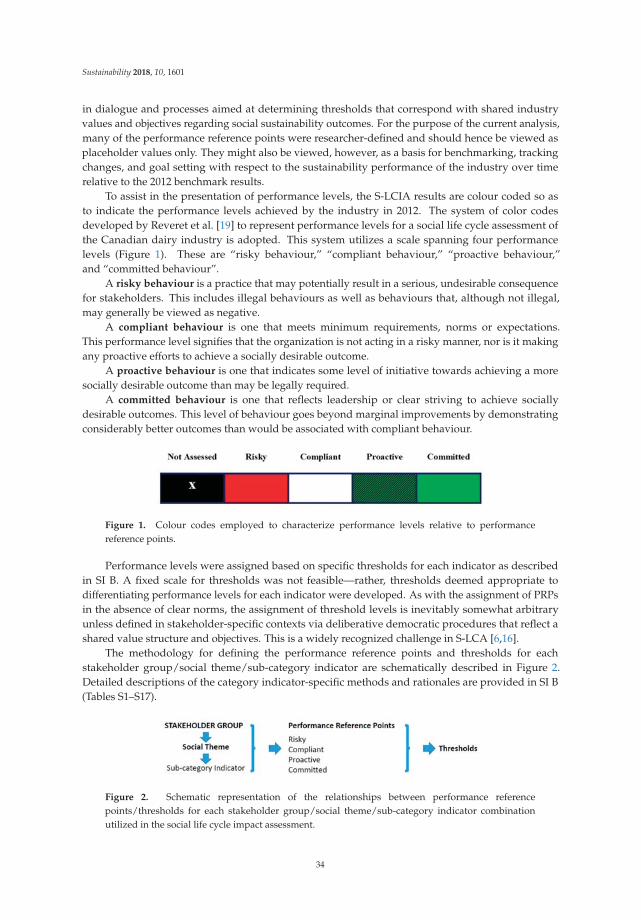
Sustainability 2018, 10, 1601
in dialogue and processes aimed at determining thresholds that correspond with shared industryvalues and objectives regarding social sustainability outcomes. For the purpose of the current analysis,many of the performance reference points were researcher-defined and should hence be viewed asplaceholder values only. They might also be viewed, however, as a basis for benchmarking, trackingchanges, and goal setting with respect to the sustainability performance of the industry over timerelative to the 2012 benchmark results.
To assist in the presentation of performance levels, the S-LCIA results are colour coded so asto indicate the performance levels achieved by the industry in 2012. The system of color codesdeveloped by Reveret et al. [19] to represent performance levels for a social life cycle assessment ofthe Canadian dairy industry is adopted. This system utilizes a scale spanning four performancelevels (Figure 1). These are “risky behaviour,” “compliant behaviour,” “proactive behaviour,”and “committed behaviour”.
A risky behaviour is a practice that may potentially result in a serious, undesirable consequencefor stakeholders. This includes illegal behaviours as well as behaviours that, although not illegal,may generally be viewed as negative.
A compliant behaviour is one that meets minimum requirements, norms or expectations.This performance level signifies that the organization is not acting in a risky manner, nor is it makingany proactive efforts to achieve a socially desirable outcome.
A proactive behaviour is one that indicates some level of initiative towards achieving a moresocially desirable outcome than may be legally required.
A committed behaviour is one that reflects leadership or clear striving to achieve sociallydesirable outcomes. This level of behaviour goes beyond marginal improvements by demonstratingconsiderably better outcomes than would be associated with compliant behaviour.
Figure 1. Colour codes employed to characterize performance levels relative to performancereference points.
Performance levels were assigned based on specific thresholds for each indicator as describedin SI B. A fixed scale for thresholds was not feasible—rather, thresholds deemed appropriate todifferentiating performance levels for each indicator were developed. As with the assignment of PRPsin the absence of clear norms, the assignment of threshold levels is inevitably somewhat arbitraryunless defined in stakeholder-specific contexts via deliberative democratic procedures that reflect ashared value structure and objectives. This is a widely recognized challenge in S-LCA [6,16].
The methodology for defining the performance reference points and thresholds for eachstakeholder group/social theme/sub-category indicator are schematically described in Figure 2.Detailed descriptions of the category indicator-specific methods and rationales are provided in SI B(Tables S1–S17).
Figure 2. Schematic representation of the relationships between performance referencepoints/thresholds for each stakeholder group/social theme/sub-category indicator combinationutilized in the social life cycle impact assessment.
34

Sustainability 2018, 10, 1601
It should also be noted that not all performance levels are relevant for all indicators. For example,if no clear norm for an indicator can be identified, then a “risky” behavior cannot be assessed.Nonetheless, it is still useful (for example, for the purpose of benchmarking or sectoral goal setting)to differentiate between the performance of companies, which may engage in socially desirablebehaviours to varying degrees, despite the lack of any clear norm or requirement.
To facilitate an accessible presentation of results in Figures 3–7, in some cases, indicator results areaggregated if the same performance score/colour code is assigned for multiple related indicators for asubcategory that can be expressed under a common indicator heading. Aggregation and weightingare not otherwise applied.
2.1.3. Interpretation and Recommendations
The Life Cycle Interpretation phase requires systematically reviewing the results of the Life CycleImpact Assessment phase with respect to the research questions. Here, the interpretation phase focusesin particular on:
• elucidating the key social risks and benefits for stakeholders that are specifically associated withactivities that occur at Canadian egg production facilities.
• identifying priority areas for interventions to improve the social license of Canadian eggproducers, either via communications regarding the social benefits associated with the eggindustry, or commitments to monitor and seek to improve the social sustainability profile ofCanadian egg production with respect to specific social risk areas.
• identifying priority areas for further data collection and research.• highlighting weaknesses of the current study and recommending areas for further research and
methods development.
3. Results
3.1. Life Cycle Inventory Results
In total, usable surveys were collected from 59 egg facilities together representing 357,286 workerhours in Canada in 2012. The number of part- and full-time workers employed in these facilities was248, with an average of 1440.7 h worked per worker per year. For detailed social life cycle inventoryresults for each indicator, see SI C Tables S18–S35, which present the social life cycle inventorydata, expressed as worker hour-weighted average results, as well as low and high reported valueswhere relevant.
3.2. Life Cycle Impact Assessment Results
Figures 3–7 present summary social life cycle impact assessment results for each stakeholdergroup, social theme and sub-category indicator. For detailed social life cycle impact assessment resultsfor each sub-category indicator, please see SI D Tables S36–S53.
STAKEHOLDER: WORKERS
Figures 3 and 4 provide a summary of LCIA results for the Workers stakeholder category.
Freedom of Association and Collective Bargaining Rights
No employers indicated that employment at their facilities is conditioned by any restrictions onthe right of employees to collective bargaining (compliant). However, for only 28% of worker hoursdid respondents indicate that employees are free to join unions of their choice. Moreover, a 0% unionrepresentation rate was reported and it would also appear that participation of employees inorganizational planning is not currently the industry norm. Only for 10% of worker hours wasit indicated that employees have access to neutral, third-party dispute resolution. Based on the current
35

Sustainability 2018, 10, 1601
Canadian average rate of union representation a risky behaviour is assessed. In light of current lackof norms but low levels of provision, compliant behaviours are assessed with respect to employeeparticipation, codified minimum notice periods regarding operational changes, and employee access toneutral, binding, and independent dispute resolution procedures. The Canadian egg industry might,however, consider options for improving employee representation and participation (SI D Table S36).
Fair Salary
Minimum wage standards were exceeded across the Canadian egg facilities surveyed for both thelowest paid and average employee, hence, on this basis, a “proactive” score is assigned. The majority(77%) of workers receive at least 10% more than the minimum wage, 41% earn at least 50% more,and 26% earn at least 100% more than the minimum wage. Relative to norms for Canadian agriculturalworkers, wages for the lowest paid employees at some Canadian egg facilities might be consideredrisky in that they are below this average. Average employee wages are, however, similar to the averagefor Canadian agricultural workers and hence a compliant score is assessed for this indicator.
Another area for improvement is with respect to the regularity and documentation of pay. For only57% of worker hours did respondents indicate that regular documentation of pay was provided. Here,a risky behaviour is assessed. There were no reported complaints regarding deductions on wages,hence a compliant behaviour is assessed for this indicator (SI D Table S37).
Figure 3. Social life cycle impact assessment scores for Canadian egg facilities in 2012 with respect tothe stakeholder group “Employees” (freedom of association and collective bargaining rights, fair salary,working hours).
36

Sustainability 2018, 10, 1601
Figure 4. Social life cycle impact assessment scores for Canadian egg facilities in 2012 with respect to thestakeholder group “Employees” (equal opportunities, health and safety, social benefits, social securityand job security).
Working Hours
The weighted average work week for employees in Canadian egg facilities in 2012 was 38.83 h,which is slightly higher than the Canadian average but much lower than the ILO maximum of 48 h(compliant behaviour). This is, however, likely consistent with working hours elsewhere in theagricultural sector. The longest average work week is 47 h (compliant behaviour). Respondents alsoindicated, however, that more than 10% of working hours correspond to work weeks in excess of48 h. Here, a risky behaviour is assessed. There is also a very low incidence of contractual agreementsregarding working hours and overtime compensation (risky behavior).
Although some employers report paying their employees a 50% overtime premium, overall,the survey data indicate a low rate of overtime pay (5.8% on average) in Canadian egg facilities.This seemingly corresponds to the norm for the Canadian agriculture sector (compliant behaviour).However, if the norm for Canadian workers as a whole is taken as the reference point, then a riskybehaviour is assessed (SI D Table S38).
Equal Opportunities
Based on reported data, employees on Canadian egg farms are largely Caucasian (97%) and male(63%), with an even age class distribution. Twenty-eight percent of respondents reported having aformal equal opportunities policy in place for their facilities (proactive behaviour). In many cases,lack of such a policy may simply reflect that the facilities are small family/owner operated facilities
37

Sustainability 2018, 10, 1601
with no other employees. However, if equality of representation of males and females is taken as theperformance reference point (compliant behaviour), or a proportionate degree of inclusion of visibleminorities (risky behaviour), then there may, indeed, be space for improvement in this regard. This issimilarly true for representation of females and visible minorities in management positions (riskybehaviour).
Considering salary equality, it would appear that male and female employees receive equalremuneration (compliant behaviour). However, female managers apparently receive lower salaries(85%) relative to male managers (risky behaviour) (SI D Table S39).
Health and Safety
According to Employment and Social Development Canada (ESDC) [21], in Canada “one in every68 employed workers in 2010 was injured or harmed on the job and received workers compensation asa result”. Although 2.7 works days were lost, on average, due to occupational accidents, injuries orillness in Canadian egg production facilities, only 0.14 WCB claims were filed per facility industry-wide,which is well below the Canadian average. No medically-diagnosed, work-related diseases or fatalitieswere reported (compliant behaviour).
Respondents indicated that 53% of worker hours occurred in workplaces characterized by highlevels of noise, fumes, or dust (risky behaviour). While all employees are provided with appropriateprotective gear when required to handle hazardous materials (committed), only half are reportedlytrained in handling such materials (proactive).
Employees generally have access to clean water and sanitary facilities (compliant behavior) and,in most cases (82% of worker hours—committed behaviour) first aid equipment is maintained andavailable to employees. A trained, designated first aid attendant was available for 62% of the reportedworker hours (proactive behaviour). A dedicated Health and Safety plan is in place for 45% of theworker hours (proactive behavior), and a dedicated Health and Safety manager for 31% of the workerhours (proactive behaviour).
Overall, it would appear that health and safety incidents were low in 2012, but that the Canadianegg industry would benefit from development and implementation of industry-wide standards withrespect to health and safety plans, management, and training. The average surveyed Canadian eggfacility invested $1762 in health and safety measures in 2012 (SI D Table S40).
Social Benefits, Social Security, and Job Security
It would appear that the provision of social benefits is not consistent within the Canadian eggindustry. Health insurance benefits are provided to less than half of employees, dental and retirementbenefits to roughly one third, and child care and/or maternity/paternity benefits to less than oneemployee in seven. Across these five categories, the average social benefit provision level is 30%.It should be noted here that some employers in Canadian egg facilities do offer full social benefits totheir employees, while others offer none.
With respect to employment contracts, only 1/4 of worker hours were subject to formalemployment contracts in 2012. Of these, roughly 2/3 were full time contracts, and 1/3 were parttime contracts. The majority of reported worker hours were not subject to an employment contract.This indicates a low level of job security. Based on a reference level of a 100% formal contract rate,a risky behavior is assessed.
According to the Conference Board of Canada (CBC) [22], the voluntary employee turn-over ratein Canada in 2012–2013 was 7.3%, and the involuntary turn-over rate was 3.7%. Employee turn-overrates in Canadian egg facilities were comparatively low (4.1% overall). Half of employees who left jobsat Canadian egg facilities in 2012 quit, while one quarter were dismissed. Compared to the Canadianaverage, a compliant behaviour is assessed (SI D Table S41).
38

Sustainability 2018, 10, 1601
STAKEHOLDER: LOCAL COMMUNITY
Figure 5 provides a summary of LCIA results for the Local Community stakeholder category.
Access to Resources
The total expenditures of egg facilities on infrastructure with mutual community access andbenefit in 2012 were very low (compliant behaviour assessed). However, some survey respondentsspent as much as $26,000 on voluntary, charitable donations and investments in their community,with an average of $2205 per facility (proactive behaviour assessed) (SI D Table S42).
Safe and Healthy Living Conditions
Only one accident in a local community was reported across surveyed facilities for 2012, hence theindustry average accident rate is very low. This single accident is taken as an outlier, hence acompliant score is assigned. However, while many facilities did not receive any complaints fromthe local community regarding nuisance issues, some facilities received as many as two complaints.Overall, 0.4 complaints were received per facility in 2012. Relative to an ideal scenario performancereference point of 0 complaints, a risky behaviour is assessed.
In light of the complaint rate, it would seem prudent to having in place formal protocols tomaintain living conditions, minimize risk, and respond to grievances in the community. Twenty-sevenpercent of facilities reported having formal protocols in place to maintain safe and healthy livingconditions, while 32% have formal protocols to minimize risk and 17% have formal protocols torespond to grievances (proactive behavior). No fines for infringements at the local level were reported(compliant behavior).
One current approach to ensuring safe and healthy living conditions in local communities andminimizing risk is the implementation of an environmental farm management plan. Two thirdsof worker hours occurred at facilities having an environmental farm management plan in 2012.Here, proactive behavior is assessed (SI D Table S43).
Respect for Indigenous Rights
While the survey data indicate that no complaints were received by Canadian egg facilities fromFirst Nations community members in 2012, it is notable that no meetings were held with First Nationsmembers. Also notable is that only 2% of worker hours were reported to occur in areas where landrights conflicts exist (risky behavior), which is unlikely to be accurate, and that only 2% of worker hoursoccurred in facilities having formal policies in place to protect the rights of indigenous communitymembers. As no norms exist in this regard, compliant behaviors are assessed. It is nonethelessrecommended that proactive behavior be encouraged in this domain (SI D Table S44).
Community Engagement
Only 7% percent of worker hours in 2012 occurred in egg facilities having formal policieson community engagement in place (compliant behavior). Reported attendance of meetings withstakeholder groups was variable, with some facilities reporting having attended as many as sixmeetings. On average, reporting facilities devoted 9 volunteer hours to community initiatives in 2012.Here, proactive behaviours are assessed (SI D Table S45).
Local Employment
Although less than 1/3 of Canadian egg facilities report having a formal policy regardinglocal hiring (proactive behavior), the local hiring rate was 87% in 2010 (committed behavior).Similarly, the majority share (64%) of goods and services purchased by egg facilities was locallysourced (proactive behavior) (SI D Table S46).
39

Sustainability 2018, 10, 1601
Figure 5. Social life cycle impact assessment scores for Canadian egg facilities in 2012 with respect tothe stakeholder group “Local Community”.
STAKEHOLDER: VALUE CHAIN PARTNERS
Figure 6 provides a summary of LCIA results for the Value Chain Partners stakeholder category.
Fair Competition
Although no facilities reported having documentation of procedures to prevent engaging in orbeing complicit in anti-competitive behaviours (compliant), no legal actions, fines or complaints werereported for 2012 (compliant) (SI D Table S47).
Promoting Social Responsibility
Three percent of worker hours occurred in facilities that report adhering to a specific code ofconduct regarding the protection of human rights (compliant behavior). No supplier audits forenvironmental or social responsibility were reported (compliant behavior). Canadian egg facilitiessurveyed for this study participated in a weighted average of 0.16 initiatives to promote value chainenvironmental or social responsibility, with a range from 0 to 5 initiatives per facility (proactivebehavior). In light of this low activity level, it would seem that there is opportunity here for initiativesto enhance the promotion of social responsibility in the Canadian egg industry (SI D Table S48).
40

Sustainability 2018, 10, 1601
Supplier Relationships
Overall, it appears that Canadian egg facilities maintain good relationships with their value chainpartners. No complaints were received from suppliers with respect to coercive communications orinsufficient lead time in 2012, and a weighted average of 0.01 complaints were received (representingone facility with two complaints, which is taken as an outlier) with respect to timeliness of payments.On the basis of this very low level, a compliant behavior is assessed for the industry as a whole (SI DTable S49).
STAKEHOLDER: SOCIETY
Figure 7 provides a summary of LCIA results for the Society stakeholder category.
Figure 6. Social life cycle impact assessment scores for Canadian egg facilities in 2012 with respect tothe stakeholder group “value chain partners”.
41

Sustainability 2018, 10, 1601
Figure 7. Social life cycle impact assessment scores for Canadian egg facilities in 2012 with respect tothe stakeholder group “Society”.
Public Commitment to Sustainability
Among those surveyed, only 8% of worker hours occurred in facilities having publicly availableCSR or other documents that communicate commitments to sustainability issues (compliant behaviour).For 1%, specific mechanisms are in place to ensure the realization of such commitments (compliantbehaviour). On this basis, it would appear that documentation and communication of sustainabilitycommitments is not currently widespread in the Canadian egg industry.
Outside of formal commitments and communications, however, some egg facilities are, indeed,engaging in sustainability initiatives. Facilities report an average of over 10 h devoted to sustainabilityprograms in 2012 (committed behavior). Some facilities were active members in programs to supportsustainable business practices (proactive behavior), and others received awards for engagement insustainability issues (proactive behavior). The average expenditure on sustainability programs was$803 (proactive behavior). No complaints were reported with respect to non-fulfillment of sustainabilitycommitments or activities to undermine sustainability measures (compliant behaviour).
In sum, it would appear that monitoring and communicating with respect to sustainability issuesis not currently the norm in the Canadian egg industry, but that some facilities are already activelyengaged in this domain. A significant opportunity may hence exist to enhance the social licenseof Canadian egg facilities through implementation and documentation of formalized sustainabilitycommitments (SI D Table S50).
42

Sustainability 2018, 10, 1601
Contribution to Economic Development
The scale of these contributions varies widely between egg facilities, reflecting the commensuratelybroad range in size of operations. For example, total revenue ranges from $260,000 to $9,464,000,with an industry average of $2,508,000 among reporting facilities. On average, participating Canadianegg facilities paid $248,000 of wages in 2012, along with $78,000 in taxes and reported an average of$1,758,000 in total expenses (SI D Table S51).
Employee Training
Significant resources were dedicated to employee training in Canadian egg facilities in 2012.On average, workers were provided with 53 h of training in 2012 (committed behaviour), and totalexpenses related to employee training averaged $529 per facility (proactive behaviour) (SI D Table S52).
Corruption
Two convictions for violations of corruption-related laws or regulations were reported by a singlefacility, with an accompanying fine of $500. This single facility report is therefore taken as an outlier, asit would appear that such violations are not commonplace within the Canadian egg industry (hencecompliant scores are assigned) (SI D Table S53).
4. Discussion
The results of this assessment provide a rich and highly nuanced characterization of the potentialsocial risks and benefits attributable to contemporary egg production facilities in Canada. They providea series of first benchmarks for the Canadian egg industry. They also highlight where and to what extentstakeholders are currently benefiting from positive social contributions made by the industry—forexample, through local job creation, high levels of employee training, provision of protective gear andfirst aid equipment for employees, and time devoted to sustainability programs (areas where facilitiesdemonstrated “committed” behaviors). These contributions go beyond what is otherwise required bylaw. The results also point towards areas of potential social risk for some stakeholders (such as thelow incidence of formal employment contracts and union representation for workers, low levels ofovertime compensation, or sub-optimal workplace diversity and equality). As such, the results suggestopportunities and strategies for the Canadian egg industry both to capitalize on its current successesas well as to proactively engage in improving its social sustainability profile.
For the “Workers” stakeholder category, the directly collected data confirmed the very low levelof representation and collective bargaining for employees of egg facilities. The representation rateof 0% was much lower than the Canadian average of 31%, but likely in-line with current norms forthe Canadian agricultural sector. Similarly, employee salaries appear to be consistent with Canadianagricultural worker norms, but lower than those of the average Canadian. Most employees are,in fact, remunerated at levels significantly higher than the minimum wage, but a small fraction ofemployees receive full- or part-time minimum wage salaries. Province-by-province assessments ofemployee wages relative to regional living wage estimates are recommended in order to ensure thatthe lowest paid employees are not at risk. Compensation for overtime pay should also be monitored,and industry-wide norms developed. On average, worker hours are within acceptable norms althougha small fraction of employees work in access of 48 hours per week. Overall, improvements with respectto formal, contractual agreements for employees regarding working conditions are recommended.
With respect to equal opportunities in the Canadian egg facility workplace, the majority ofemployees are currently Caucasian males. Visible minorities have a very low level of representation inthis workforce. For general employees, salaries are equitable for males and females. However, the datacollected for 2012 suggest a disparity in pay for female compared to male managers of roughly 15%.Additional research and possible mitigation strategies may be desirable to increase diversity andensure equality for employees.
43
Sustainability 2018, 10, 1601
Health and safety conditions for workers in Canadian egg facilities appear to be very good.Although facilities are often characterized by high levels of dust and/or noise, employers report highlevels of worker training, use of protective gear, and access to first aid equipment and sanitary facilities.Many facilities report the use of dedicated health and safety plans, as well as designated first aidattendants. No medically-diagnosed, workplace-related diseases or fatalities were reported for 2012.
Provision of social benefits to workers varies widely between egg facilities. Many facilities reportproviding at least one non-mandatory social benefit and some more than three. Others provide noadditional benefits to employees. This suggests opportunities for the development of norms withinthe Canadian egg industry to promote consistent provision of non-mandatory social benefits in orderto improve conditions for employees. Improving job security through the implementation of formalemployment contracts is also recommended, as current usage of contractual agreements is low.
For the stakeholder group “Local Community,” it would appear that Canadian egg facilitiesare often proactively engaged in making meaningful contributions to the communities in whichthey operate. Egg facilities largely employ local community members, and source a large fraction ofinputs from local businesses. Most facilities reported some level of voluntary, charitable donationsor investments in their communities, with an average of $2205 spent on local community initiativesper facility in 2012. Participation in community initiatives is also high. In addition, many facilitiesreport implementation of an Environmental Farm Management Plan, which serves to reduce risk ofnuisance issues, as well as the existence of formal protocols to mitigate risk for local communitiesand respond to grievances. The overall accident rate in local communities as a result of egg facilityactivities was very low. One area of potential social risk relates to interactions with indigenouscommunities. Although many egg facilities are situated in communities proximate to First Nationscommunities, only 2% reported operating in areas where land rights conflicts exist, and reported levelsof proactive engagement with First Nations communities were low. Formalizing “good neighbour”policies and outreach may be desirable. This could potentially be paired with initiatives to increaseworkplace diversity.
Management decisions and activities similarly impact on society at large, and may resultin either societal risks or benefits. Demonstrating commitment to and actions consistent withcontributing positively to society is fundamental to the concept of corporate social responsibility(CSR). CSR reporting, including transparent mechanisms for measuring, monitoring, goal settingand follow-up, is increasingly important to maintaining social license, as well as accessing emergingmarket opportunities associated with sustainability objectives.
Many Canadian egg facilities are already taking steps to improve and promote the sustainabilityof their practices. Facilities reported an average of 10 h devoted to sustainability initiatives in 2012,and related expenses of roughly $800 per facility. Development and reporting of formal CSR documentsis, however, relatively uncommon. An industry-wide initiative to support operators in developing andimplementing CSR strategies is strongly encouraged. Indeed, in light of increased attention by bothcommodity groups and large retailers to developing and implementing sustainability measurement,reporting and certification requirements, it is strongly recommended that the Canadian egg industrybecome proactive in this respect. This will require the support and cooperation of both producers andtheir representative bodies in order to develop and implement industry-wide strategies and initiatives.
Social life cycle assessment is a relatively new field of research, and methodological developmentis on-going. To date, very few social LCA studies of food products have been reported (for example,see [11,13,14,19,23,24]). Varied approaches have often been employed [11,12] and, given the diversityof agri-food production contexts, the feasibility and desirability of consistency between studiesis debatable.
The current analysis represents only a partial (i.e., gate-to-gate) evaluation of the potential socialrisks and benefits attributable to the Canadian egg industry. Future work should expand the analysisto encompass value chain stages and stakeholder interactions both upstream and downstream ofCanadian egg facilities. While considerable efforts were invested to ensure appropriate representation
44

Sustainability 2018, 10, 1601
across regions of production (provinces) and farm size, the sample nonetheless represents a relativelysmall subset of egg production facilities in Canada. In this respect, “scaling up” results is challenging,and collecting larger data samples wherever feasible in such analyses is clearly desirable. The surveyquestions (and related indicators that can be assessed) should also be periodically revisited so as toensure that all relevant social sustainability issues are taken into consideration—in particular giventhat conditions may change over time, and the suite of social sustainability issues deemed appropriatefor inclusion in such analyses will likely continue to evolve. Moreover, while the impact assessmentmethods that were developed here provide a valuable example of how social risks and benefits mightbe assessed in egg production or for other food production activities, it is important to note thatdefining performance reference points for social life cycle impact assessment where clear norms do notexist is challenging and inevitably somewhat arbitrary. This is similarly true with respect to identifyingappropriate thresholds for distinguishing between levels of “sustainability performance” for eachindicator considered, even where norms do exist. Multiple, competing bases are possible. For thisreason, it is essential that methods and data are transparently presented so as to enable identificationof potential real or perceived bias. Moreover, it may be preferable to present results at the indicatorlevel (as in the current study) rather than aggregating results across indicators, since such aggregationrequires weighting (introducing an additional level of uncertainty and potential bias) and may alsobias interpretation if numerous “easy to achieve” norms outweigh a limited number of more importantsocial sustainability performance indicators.
Clearly, a desirable next step, in the extension of this methods development and analysisexercise, is for the Canadian egg industry to engage in a multi-stakeholder dialogue in order todefine mutually agreed upon, clear thresholds for performance levels as well as goals for socialsustainability performance in this industry [13]. The novel set of social sustainability metrics developedhere can therefore provide a useful starting point for continued development and application in theCanadian egg sector and may be usefully adapted for application in other agri-food sectors in Canadaand beyond.
Supplementary Materials: The following are available online at http://www.mdpi.com/2071-1050/10/5/1601/s1, SI A—Social Life Cycle Inventory Survey, SI B—Social Life Cycle Impact Assessment Indicators andPerformance Reference Points, SI C—Detailed Social Life Cycle Inventory Results, and SI D—Detailed Social LifeCycle Impact Assessment Results.
Funding: This research was funded by Egg Farmers of Canada. Publication was supported through theNSERC/Egg Farmers of Canada Industrial Research Chair in Sustainability.
Conflicts of Interest: The author declares no conflict of interest. The funding sponsors had no role in the designof the study; in the collection, analyses, or interpretation of data; in the writing of the manuscript, and in thedecision to publish the results.
References
1. Pelletier, N.; Sala, S.; Ostaglu, E.; Rosenbaum, E.; Vasta, A.; Benoit-Norris, C.; Norris, G. Social sustainabilityin trade and development policy. Int. J. Life Cycle Assess. 2018, 23, 629–639. [CrossRef]
2. Jorgensen, A.; Le Bocq, A.; Nazarkina, L.; Hauschild, M. Methodologies for social life cycle assessment. Int. J.Life Cycle Assess. 2008, 13, 96–103. [CrossRef]
3. Jorgensen, A.; Lai, L.; Hauschild, M. Assessing the validity of impact pathways for child labour and wellbeingin social life cycle assessment. Int. J. Life Cycle Assess. 2010, 15, 5–16. [CrossRef]
4. Jorgensen, A. Social LCA—A way ahead? Int. J. Life Cycle Assess. 2013, 18, 296–299. [CrossRef]5. Zamagni, A.; Feschet, P.; De Luca, A.; Iofrida, N.; Buttol, P. Social Life Cycle Assessment: Methodologies
and Practice. In Sustainability Assessment of Renewables-Based Products: Methods and Case Studies; Dewulf, J.,De Meester, S., Rodrigo, A., Eds.; Wiley: New York, NY, USA, 2015; Available online: http://ca.wiley.com/WileyCDA/WileyTitle/productCd-111893394X.html# (accessed on 5 January 2017).
6. UNEP/SETAC. Guidelines for Social Life Cycle Assessment of Products. In The UNEP/SETAC Life CycleInitiative; UNEP/SETAC: Paris, France, 2009.
45

Sustainability 2018, 10, 1601
7. Benoit-Norris, C.; Norris, G.; Valdivia, S.; Ciroth, A.; Moberg, A.; Bos, U.; Prakash, S.; Ugaya, C.; Beck, T.The guidelines for social life cycle assessment of products: Just in time! Int. J. Life Cycle Assess. 2010, 15,156–163. [CrossRef]
8. Do Carmo, B.; Margni, M.; Baptiste, P. Addressing uncertain scoring and weighting factors in social life cycleassessment. Int. J. Life Cycle Assess. 2017, 22, 1609–1617. [CrossRef]
9. Wu, R.; Yang, D.; Chen, J. Social life cycle assessment revisited. Sustainability 2014, 6, 4200–4226. [CrossRef]10. Iofrida, N.; De Luca, A.; Strano, A.; Gulisano, G. Can social research paradigms justify the diversity of
approaches to social life cycle assessment? Int. J. Life Cycle Assess. 2018, 23, 464–480. [CrossRef]11. Paragahawewa, U.; Blackett, P.; Small, B. Social Life Cycle Analysis (S-LCA): Some Methodological Issues and
Potential Application to Cheese Production in New Zealand; AgResearch Ltd.: Palmerston North, New Zealand,2009.
12. Smith, J.; Barling, D. Social impact and life cycle assessment: Proposals for methodological development forSMEs in the European food and drink sector. Int. J. Life Cycle Assess. 2014, 19, 944–949. [CrossRef]
13. De Luca, A.; Iofrida, N.; Strano, A.; Falcone, G. Social life cycle assessment and participatory approaches:A methodological proposal applied to citrus farming in Southern Italy. Integr. Environ. Assess. 2015, 11,383–396. [CrossRef] [PubMed]
14. Chen, W.; Holden, N. Social life cycle assessment of average Irish dairy farm. Int. J. Life Cycle Assess. 2017,22, 1459–1472. [CrossRef]
15. Petti, L.; Ramirex, P.; Traverso, M.; Ugaya, C. An Italian tomato “Cuore di Bue” case study: Challenges andbenefits of using subcategory assessment method for social life cycle assessment. Int. J. Life Cycle Assess.2018, 23, 569–580. [CrossRef]
16. Benoît-Norris, C.; Vickery-Niederman, G.; Valdivia, S.; Franze, J.; Traverso, M.; Ciroth, A.; Mazijn, B.Introducing the UNEP/SETAC methodological sheets for subcategories of social LCA. Int. J. Life Cycle Assess.2011, 16, 682–690. [CrossRef]
17. Spillemaecker, S.; Vanhoutte, G.; Traverniers, L.; Lavrysen, L.; van Braeckel, D.; Mazijin, B.; Rivera, J.Integrated Product Assessment: The Development of the Label ‘Sustainable Development’ For Products, Ecological,Social, and Economical Aspects of Integrated Product Policy; Belgian Science Policy: Brussels, Belgium, 2004.
18. Dreyer, L.; Hauschild, M.; Schierbeck, J. Characterisation of social impacts in LCA. Int. J. Life Cycle Assess.2010, 15, 247–259. [CrossRef]
19. Reveret, J.P.; Couture, J.M.; Parent, P. Socio-economic LCA of milk production in Canada. In Social Life CycleAssessment; Muthu, S., Ed.; Springer Science + Business Media: Singapore, 2015. [CrossRef]
20. AAFC. Canada’s Poultry and Egg Industry Profile at a Glance; Agriculture and Agri-Food Canada: Ottawa, ON,Canada, 2013.
21. ESDC. Work—Work-Related Injuries. Indicators of Well-Being in Canada; Employment and Social DevelopmentCanada: Toronto, Canada, 2015. Available online: http://www4.hrsdc.gc.ca/[email protected]?iid=20(accessed on 10 June 2016).
22. CBC. What Are the Overall Voluntary and Involuntary Turnover Rates for Canadian Organizations? HR Questionsand Answers; Conference Board of Canada: Ottawa, ON, Canada, 2015; Available online: http://www.conferenceboard.ca/topics/humanresource/questions.aspx#Q1 (accessed on 10 June 2016).
23. Kruse, S.; Flysjo, A.; Kasperczyk, N.; Scholz, A. Socioeconomic indicators as a complement to life cycleassessment—An application to salmon production systems. Int. J. Life Cycle Assess. 2009, 14, 8–18. [CrossRef]
24. Manik, Y.; Leahy, J.; Halog, A. Social life cycle assessment of palm oil biodiesel: A case study in JambiProvince of Indonesia. Int. J. Life Cycle Assess. 2013, 18, 1386–1392. [CrossRef]
© 2018 by the author. Licensee MDPI, Basel, Switzerland. This article is an open accessarticle distributed under the terms and conditions of the Creative Commons Attribution(CC BY) license (http://creativecommons.org/licenses/by/4.0/).
46

sustainability
Article
Study on the Vertical Linkage of Greenhouse GasEmission Intensity Change of the Animal HusbandrySector between China and Its Provinces
Tianyi Cai 1,2, Degang Yang 1,* ID , Xinhuan Zhang 1, Fuqiang Xia 1 and Rongwei Wu 1,2 ID
1 Xinjiang Institute of Ecology and Geography, Chinese Academy of Sciences, Urumqi 830011, China;[email protected] (T.C.); [email protected] (X.Z.); [email protected] (F.X.);[email protected] (R.W.)
2 University of Chinese Academy of Sciences, Beijing 100049, China* Correspondence: [email protected]; Tel.: +86-0991-7827319
Received: 30 May 2018; Accepted: 13 July 2018; Published: 16 July 2018
Abstract: China’s carbon intensity (CI) reduction target in 2030 needs to be allocated to each provincein order to be achieved. Thus, it is of great significance to study the vertical linkage of CI changebetween China and its provinces. The existing research on the vertical linkage focuses more onenergy-related economic sectors in China; however, attention has not been paid to China’s animalhusbandry (AH) sector, although the role of the China’s AH sector in greenhouse gas (GHG) reductionis increasingly important. This study firstly established a vertical linkage of change in greenhousegas emission intensity of the animal husbandry sector (AHGI) between China and its 31 provincesbased on the logarithmic mean Divisia index (LMDI) decomposing method from the perspectiveof combining emission reduction with economic development, and quantified the contributions ofeach province and its three driving factors of environmental efficiency (AHEE), productive efficiency(AHPE), and economic share (AHES) to reducing China’s AHGI during the period of 1997–2016.The main results are: (1) The AHGI of China decreased from 5.49 tCO2eq/104 yuan in 1997 to2.59 tCO2eq/104 in 2016, showing a 75.25% reduction. The AHGI in 31 provinces also declinedand played a positive role in promoting the reduction of national AHGI, but there were significantinter-provincial differences in the extent of the contribution. Overall, the provinces with higheremission levels contributed the most to the reduction of China’s AHGI; (2) The AHPE and AHEEfactors in 31 provinces cumulatively contributed to the respective 68.17% and 11.78% reduction ofChina’s AHGI, while the AHES factors of 31 provinces cumulatively inhibited the 4.70% reduction.Overall, the AHPE factor was the main driving factor contributing to the reduction of China’sAHGI. In the future, improving the level of AHEE through GHG emissions reduction technology andnarrowing the inter-provincial gap of the level of AHPE are two important paths for promoting thereduction of China’s AHGI.
Keywords: LMDI; provincial contribution; emission reduction; decomposition; driving factor
1. Introduction
In 2015, at the “Paris Climate Conference”, the international community reached a legally-bindingtarget of limiting the global temperature increase to no more than 2 ◦C [1]. To attain this target, globalgreenhouse gas (GHG) emissions must be reduced by 70% by 2050 [2]. Moreover, the implementationof effective emission reduction depends on the emission reduction policies and cooperation of differentcountries and their economic sectors [3]. China is the world’s largest emitter of GHG and largestdeveloping country [4]. The Chinese government had integrated emission reduction with economicdevelopment and promised the world that by 2030 the CO2 emission intensity of its GDP would be
Sustainability 2018, 10, 2492; doi:10.3390/su10072492 www.mdpi.com/journal/sustainability47

Sustainability 2018, 10, 2492
reduced by 60–65% compared to 2005 levels [5]. Meanwhile, this carbon intensity (CI) reduction targetwas allocated to each province in order to be achieved [6–8].
However, China’s daunting CI reduction target is only intended for CO2 emissions, with noclear quantitative target for non-CO2 GHG emission reduction [4]. In fact, non-CO2 GHG emissionsare an important contributor to global warming [9], and the animal husbandry (AH) sector has beenuniversally recognized as the primary source of global non-CO2 GHG (CH4 and N2O) emissions [9–13].Non-CO2 emissions directly from the AH sector contribute approximately 19% to the current climatewarming [14], but there is also very large potential for emission reduction [10,15–18]. China’s AH sectoremitted 445 million tons (2005) of non-CO2 GHG (CO2 equivalents), accounting for approximately 6%of China’s total GHG emissions and 30% of the total non-CO2 GHG emissions [19]. With the continuousrise in the per capita income level and the continuous progress in urbanization in China, the demandfor livestock food in the residents’ diet will continue to grow [20–24]. Thus, the AH sector will playa more important role in reducing GHG emissions in China. China’s CI reduction targets need to beallocated to each province to achieve. Therefore, it is of great significance to conduct a study from theperspective of combining emissions reduction with economic development to uncover the verticallinkage of change in greenhouse gas emission intensity of animal husbandry sector (AHGI) betweenChina and its provinces, and evaluate the driving factors of change in AHGI, which will provide animportant basis for formulating provincial AHGI reduction targets for China.
Macro studies on global GHG emission intensity of AH sector have been reported. Caro’s studyfound that it was vastly different among countries of the intensity of GHG emission per unit ofeconomic output value in AH sector in 2010, with the highest intensity occurring in developingcountries, and particularly Africa [11]. Bennetzen’s study showed that GHG emissions per unitlivestock product has decreased by approximately 44% since 1970 in global. The decoupling oflivestock production and emissions had shown very large regional differences. While developingcountries have contributed to the doubling of global livestock production, they have also contributedmore GHG emissions [25,26]. However, more literature has focused on the study of the carbon footprintof animal products from a small scale perspective [27–32].
Existing studies on the vertical linkage and its drivers of CI between China and its provinces havemainly focused on energy-related CO2 emission intensity [7,33–35], with the logarithmic mean Divisiaindex (LMDI) approach being the most commonly used decomposition method. Wang et al. [7] used theLMDI method to investigate the contribution given by China’s 30 provinces to the decline of nationalCI from 1997 to 2008. The results showed that Liaoning, Heilongjiang, and Hebei have made greatercontributions to the decline of national CI, the contribution of a province to the decline of national CIlaid mainly in the promotion of its energy efficiency. Zhang et al. [33] applied the LMDI technique toexplore the CI drivers in 29 Chinese provinces from 1995 to 2012. The results indicated that the overallCI of China decreased rapidly and energy intensity is the most significant driver for the decrease of CI.Tan et al. [34] examined the role of activities related to the electric power industry in reducing China’sCI from 1998 to 2008 utilizing the LMDI technique. The results revealed that the provinces with higheremission levels contributed the most to China’s improvements in CI. Wang et al. [35] established paneldata models to explore the influencing factors of CI in China. The results showed that the economiclevel of activity was negatively correlated to CI on both national and regional levels. However,attention has not been paid to China’s AH sector. The existing research literature related to China’s AHsector have either focused more on the macro horizontal perspective on the regional characteristics ofemissions and intensity in various provinces [36–39] and the decomposition of the drivers for carbonemissions [39–43], or on the micro perspective on the differences in the carbon footprint betweendifferent feeding methods [44,45] and different animal products [46–48]. Meng et al. [36] estimatedthe AH’s GHG emissions of China’s different livestock division by life circle assessment method.The results revealed that there were higher emissions of CO2 equivalent of livestock in agriculturalareas than in pastoral areas, but the emission intensity was lower than in pastoral areas. Yao et al. [37]used the same method to obtain a conclusion that high livestock carbon emissions areas were mostly
48

Sustainability 2018, 10, 2492
located in prairie areas or major grain producing areas of China. Luo et al. [38] explored the spatialand temporal heterogeneity of CO2 emission intensity in China’s agricultural sector and found thatCentral China had the highest agricultural CO2 emission intensity than Western and Eastern China.Tian et al. [39,41] studied regional characteristics and driving factor of agricultural carbon emissions inChina with LMDI model. The results showed that the traditional agricultural provinces, especially themajor crop production areas were the main emission source regions. The efficiency factor, labor factor,and industry structure factor had strong inhibitory effects on China’s agricultural carbon emissions,while the economy factor had a strong positive effect. Yao et al. [43] conducted a decomposition studyon the factors affecting the changes of AH carbon emissions based on the LMDI method and foundthat AH production efficiency improvement was the most important factor to restrain the sustainedgrowth of the AH carbon emissions. Xiong et al. [40,42] used the same decomposition method to drawconclusions that the economy factor was the critical factor to promote the increase in agriculturalcarbon emissions in Xinjiang province of China, while the main inhibiting factor was the efficiencyfactor. These research results have enriched the body of work on GHG emissions reduction in China’sAH sector from different perspectives. However, the above-mentioned studies have mostly treated boththe AH sector and crop farming sector as part of the agricultural sector and neglected the particularityof the AH sector. In fact, first of all, the AH sector differs from the crop farming sector in its productionmethods, the economic benefits, the generation mechanism of GHG, and the emission reductionstrategies; secondly, studying the GHG emissions and intensity of the AH sector from the horizontalperspective of provinces cannot reveal the vertical linkage between the partial and overall changes.More importantly, vertical linkage is an important basis for the Chinese government to formulateAHGI reduction targets for all provinces.
Our work is different from the above research in the following respects: First, this studyestimated the GHG emissions (CO2 equivalent) per unit of AH economic output value in China and its31 provinces from 1997 to 2016. Second, we established a vertical linkage of change in AHGI betweenchina and its 31 provinces from the perspective of combining emissions reduction with economicdevelopment, and separated the factors affecting the change of AHGI into environmental efficiency,productive efficiency and economic share. We used the LMDI decomposition method to supportour study, because it was proven to be a feasible tool in achieving complete decomposition withoutresiduals, allowing subgroup estimations to be aggregated in a consistent manner and performingattribution analyses on the impact of subcategory estimates [49]. Third, we quantified the contributionsof each province and its three driving factors to the change of China’s AHGI during the period of1997–2016. This study aims to provide a reference for formulating provincial AHGI reduction targetsfor the Chinese government in a more scientific and reasonable way.
2. Materials and Methods
2.1. Estimation of AHGI
This study adopted the GHG emissions (CO2 equivalent) per unit of the AH economic outputvalue as the AHGI indicator. The formula is shown as follows:
AHGI = AHGE/AHGDP (1)
where AHGI, AHGE, and AHGDP denote greenhouse gas emission intensity of animal husbandrysector (in tCO2eq/104 yuan), the sum of greenhouse gas emissions from animal husbandry sector(in tCO2eq) and economic output value of animal husbandry sector (104 yuan), respectively. The AHGIof each province is calculated similarly.
According to the “Guidelines for Compiling Low-carbon Development and Provincial GreenhouseGas Inventory” issued by the Department of Climate Change of the National Development and ReformCommission of China (NDRCC) in 2013 [50], the provincial GHG inventory for AH includes two parts:CH4 and N2O emissions in animal manure management and CH4 emissions from animal enteric
49

Sustainability 2018, 10, 2492
fermentation in this study. Due to the vast territory of China, the climate and soil conditions indifferent geographical regions have different effects on CH4 and N2O emissions during the storage andmanagement of animal manure, so the emissions factors of different emission sources also adopt therecommended values of the sub-regions in China by the guidelines. The formula is shown as follows:
AHECH4,manure =(∑ APi × EFCH4,manure,i
)× 10−3 (2)
AHEN2O,manure =(∑ APi × EFN2O,manure,i
)× 10−3 (3)
AHECH4,enteric =(∑ APi × EFCH4,enteric,i
)× 10−3 (4)
AHGE =[(
AHECH4,manure + AHECH4,enteric)× 25 + AHEN2O,manure × 298
](5)
where AHECH4,manure represent the sum of the CH4 caused by the manure management, in t CH4/year;AHEN2O,manure represent the sum of the N2O emissions caused by the manure management, in tN2O/year; AHECH4,enteric represents the sum of the CH4 emissions caused by enteric fermentation,in t CH4/year; APi is the amount of annual feeding of animal i in head; i include cattle, buffalo,dairy cows, horses, donkeys, mules, camels, goats, sheep, pigs and poultry in China; Non-ruminantanimals, especially poultry, which have small body weights, produce low CH4 emissions. Therefore,CH4 emissions from non-ruminant animals are not included in animal enteric fermentation emissions;EFCH4,manure ,i is the CH4 emission factor of manure management of animal i in kg CH4/head/year,as shown in Table A1; and EFN2O,manure ,i is the N2O emission factor of manure management of animali in kg N2O/head/year, as shown in Table A2; EFCH4,enteric ,i is the CH4 emission factor of entericfermentation of animal i, in kg CH4/head/year. The guidelines give the methane emission factors forenteric fermentation of different animals in different feeding modes (large-scale farming, farmer raising,and grazing) in China. However, it is difficult to obtain the provincial data of livestock activity bydistinguishing different feeding methods, so the CH4 emission factor for animal enteric fermentation inthis study uniformly adopted IPCC recommendations [51] as shown in Table 1, in kg CH4/head/year.In order to facilitate the summation of total greenhouse gas emissions and comparative analysis ineach province, we converted CH4, N2O to CO2 equivalent. 25 and 298 are the relative molecularwarming forcing of CH4 and N2O in a 100-year horizon, respectively [52]. AHGE represent the sumof greenhouse gas emissions from animal husbandry sector, in tCO2eq. The AHGE of each provinceis calculated similarly. The total amount of AHGE in China is equal to the sum of total AHGE in31 provinces.
Table 1. The CH4 emission factor for animal enteric fermentation (kg CH4/head/year).
Livestock Emission Factor Livestock Emission Factor Livestock Emission Factor
Buffalo 55 Mule 10 Sheep 5Dairy cow 61 Camel 46 Goat 5
Cattle 47 Horse 18 Pig 1Donkey 10
2.2. Decomposition of AHGI
2.2.1. Decomposing Process
As the total AHGE and AHGDP from China are generated by the AH sectors of the 31 provincesacross the country, this study firstly established a vertical linkage of the AHGI calculation between thenational and provincial AH sectors. The calculation is shown as follows:
AHGI =AHGE
AHGDP=
31
∑i=1
AHGEi/31
∑i=1
AHGDPi (6)
50
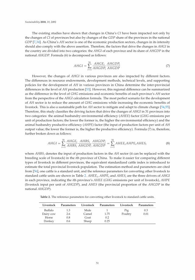
Sustainability 2018, 10, 2492
The existing studies have shown that changes in China’s CI have been impacted not only bythe changes of CI of provinces but also by changes of the GDP share of the provinces in the nationalGDP [7,34]. As China’s AH sector is one of the economic production sectors, changes in its intensityshould also comply with the above assertion. Therefore, the factors that drive the changes in AHGI inthe country are divided into two categories: the AHGI of each province and its share of AHGDP in thenational AHGDP. Formula (6) is decomposed as follows:
AHGI =31
∑i=1
AHGEiAHGDPi
AHGDPiAHGDP
(7)
However, the changes of AHGI in various provinces are also impacted by different factors.The differences in resource endowments, development methods, technical levels, and supportingpolicies for the development of AH in various provinces in China determine the inter-provincialdifferences in the level of AH production [53]. However, this regional difference can be summarizedas the difference in the level of GHG emissions and economic benefits of each province’s AH sectorfrom the perspective of the AHGI calculation formula. The most perfect scenario for the developmentof AH sector is to reduce the amount of GHG emissions while increasing the economic benefits oflivestock. This is also a sustainable path for AH sector to mitigate and adapt to climate change [54,55].Therefore, this study classifies the driving factors that drive the changes of AHGI in 31 provinces intotwo categories: the animal husbandry environmental efficiency (AHEE) factor (GHG emissions perunit of production factors; the lower the former is, the higher the environmental efficiency) and theanimal husbandry productive efficiency (AHPE) factor (the input of production factors per unit of AHoutput value; the lower the former is, the higher the productive efficiency). Formula (7) is, therefore,further broken down as follows:
AHGI =31
∑i=1
AHGEiAHBSi
AHBSiAHGDPi
AHGDPiAHGDP
=31
∑i=1
AHEEi AHPEi AHESi (8)
where AHBSi denotes the input of production factors in the AH sector (it can be replaced with thebreeding scale of livestock) in the ith province of China. To make it easier for comparing differenttypes of livestock in different provinces, the equivalent standardized cattle index is introduced toestimate the total provincial livestock population. The estimation method and parameters are citedfrom [56], one cattle is a standard unit, and the reference parameters for converting other livestock tostandard cattle units are shown in Table 2. AHEEi, AHPEi and AHESi are the three drivers of AHGIin each province, indicating the ith province’s AHEE (GHG emissions per unit of livestock), AHPE(livestock input per unit of AHGDP), and AHES (the provincial proportion of the AHGDP in thenational AHGDP).
Table 2. The reference parameters for converting other livestock to standard cattle units.
Livestock Parameters Livestock Parameters Livestock Parameters
Buffalo 1.3 Mule 1 Pig 0.3Dairy cow 2.6 Camel 1.75 Poultry 0.01
Horse 0.8 Goat 0.2Donkey 0.6 Sheep 0.25
51

Sustainability 2018, 10, 2492
2.2.2. Calculating Method
After decomposing the AHGI into the above three driving factors, as shown in Equation (8),next we will present the method used to calculate. Referring to Ang [49], the change of AHGI can bedecomposed using an additive LMDI method as follows:
lnAHGITAHGI0
= ΔAHGI = AHGIT − AHGI0 = ΔAHEE + ΔAHPE + ΔAHES (9)
where T represents the end of the period; 0, the start of the period; ΔAHGI, the change of AHGI inChina; ΔAHEE, the contribution of AHEE factor; ΔAHPE, the contribution of AHPE factor; and ΔAHES,the contribution of AHES factor. ΔAHEE, ΔAHPE and ΔAHES can be calculated by:
ΔAHEE =31
∑i=1
wAH∗i ln(AHEEi,T/AHEEi,0) (10)
ΔAHPE =31
∑i=1
wAH∗i ln(AHPEi,T/AHPEi,0) (11)
ΔAHES =31
∑i=1
wAH∗i ln(AHESi,T/AHESi,0) (12)
where wAH∗i in the above equations is the logarithmic weighting scheme specified in the following:
wAH∗i = L
(wAH
i,0 , wAHi,T
)/
31
∑i=1
L(
wAHi,0 , wAH
i,T
)(13)
L(
wAHi,0 , wAH
i,T
)=
(wAH
i,T − wAHi,0
)/ln
(wAH
i,T /wAHi,0
)(14)
wAHi = AHEEi AHPEi AHESi/
31
∑i=1
AHEEi AHPEi AHESi (15)
2.3. Data Collection and Processing
This study involves 31 provinces in mainland China and the study period spans from 1997 to2016. Considering the feeding cycles which are more than one year of cattle, buffalo, dairy cows,horses, donkeys, mules, goats, and sheep [51], the data for the annual total livestock raised is denotedby the year-end inventory data. The feeding cycle for poultry (55 days) and pig (200 days) is lessthan one year [37], and the data for the annual total is expressed by the current year’s slaughtervolume [53]. The time-series livestock activity data of each province used in this paper are obtainedfrom the China Rural Statistical Yearbook (1998–2017). The time-series livestock economic output dataof every province are obtained from the China Statistical Yearbook (1998–2017) and then converted tooutputs in constant 1997 price. All abbreviations used in this study are described in Table A3.
As China’s CI reduction target is a long-term target, until 2030, this study took 1997 as the baselineperiod and 2016 as the comparison period as the basis for this research.
3. Results and Discussion
3.1. Changes of AHGI in China and Its Provinces
From a national perspective, the AHGI of China decreased from 5.49 tCO2eq/104 yuan in 1997 to2.59 tCO2eq/104 in 2016, showing a 75.25% reduction within this period, as shown in Figure 1. This is inline with the finding by Caro [11] that the AHGI in global developing countries has been on the decline.
52

Sustainability 2018, 10, 2492
From a provincial perspective, compared 2016 with 1997, the AHGI were all decreasing in31 provinces, but the extent of the decrease varied significantly among the provinces. Figure 2 showsthat the AHGI in 15 provinces (including Hainan, Heilongjiang, Yunnan, Anhui, Henan, Guizhou,Shanxi, Hebei, Shaanxi, Guangxi, Xinjiang, Inner Mongolia, Jilin, Shandong and Sichuan) declinedfaster than 75.25% (the aggregate reduction in AHGI of China), while the AHGI in other 16 provincesdeclined slower than 75.25%. Hainan’s AHGI declined from 6.68 tCO2eq/104 yuan to 1.76, which wasthe largest decline (133.28%) of all the provinces. Liaoning’s AHGI declined from 3.11 tCO2eq/104 yuanto 2.54, which was the smallest decline (19.91%) of all the provinces.
According to the above changing trends of the AHGI in China and its provinces during theperiod of 1997–2016, this paper argues that these reductions of the AHGI are due to two reasons.On the one hand, the AHGE has been growing slowly with the transformation of China’s AHproduction from an extensive mode to an intensive mode during the study period. On the other hand,the AHGDP has been growing rapidly due to advancement of livestock feeding and managementtechniques, and standardization, scale, and organizational level of AH production. However, there aresignificant inter-provincial differences in resource endowments, development methods, technical levels,and supporting policies for the development of AH, which made the extent of reduction differentamong the 31 provinces.
0.0
1.0
2.0
3.0
4.0
5.0
6.0
1997
1998
1999
2000
2001
2002
2003
2004
2005
2006
2007
2008
2009
2010
2011
2012
2013
2014
2015
2016
AH
GI (
tCO
2eq
/104
Yuan
)
Year
Figure 1. Changes of AHGI in China during the period 1997–2016.
-140.00
-120.00
-100.00
-80.00
-60.00
-40.00
-20.00
0.00
Hen
anH
ebei
Shan
dong
Sich
uan
Gua
ngxi
Hun
anA
nhui
Yunn
anG
uang
dong
Hub
eiG
uizh
ouJia
ngxi
Tibe
tXi
njia
ngIn
ner M
ongo
liaJia
ngsu
Hei
long
jiang
Qin
ghai
Shan
xiJil
inSh
aanx
iG
ansu
Cho
ngqi
ngZh
ejia
ngFu
jian
Hai
nan
Shan
ghai
Liao
ning
Beiji
ngN
ingx
iaTi
anjin
∆AH
GI (
%)
∆AHGI of Province ∆AHGI of China
Figure 2. Changes of AHGI in 31 provinces, comparing 2016 with 1997.
It was reported that 445 million tCO2eq were emitted from animal enteric fermentation andmanure management in the Second National Communication on Climate Change (NCCC) issued bythe Chinese government in 2005, using 21 and 310 as the values for Global Warming Potential (GWP)
53

Sustainability 2018, 10, 2492
of CH4 and N2O [19]. Our estimates of 503 million tCO2eq emissions for the corresponding year arecomparable to these data and differences can be attributed to different GWP (this paper used IPCCFourth Assessment Report value (25 and 298 of CH4 and N2O)) [52]. However, this will not affect theoverall research results and, thus, the estimated value of AHGI used in this study is reliable.
3.2. Analysis of Provincial Contributions to the Reduction of China’s AHGI
Compared 2016 with 1997, China’s AHGI showed a 75.25% reduction. The decompositionresults (Table 3, Figure 3) of provincial contributions from the LMDI model showed that all provincesplayed a positive role in promoting the 75.25% reduction of China’s AHGI, but there were significantdifferences among provinces in the extent of the contribution. The top 10 contributing provinceswere Henan (−7.11%), Hebei (−5.58%), Shandong (−5.55%), Sichuan (−5.29%), Guangxi (−4.81%),Hunan (−4.29%), Anhui (−4.24%), Yunnan (−3.31%), Guangdong (−3.23%), and Hubei (−2.82%),while the bottom ten contributing provinces, in descending order, were Tianjin (−0.06%), Ningxia(−0.14%), Beijing (−0.34%), Liaoning (−0.35%), Shanghai (−0.58%), Hainan (−0.59%), Fujian (−1.01%),Zhejiang (−1.01%), Chongqing (−1.12%), and Gansu (−1.25%). Considering the largest and smallestcontributors, Henan contributed approximately 119 times as much as Tianjin.
-8.00-7.00-6.00-5.00-4.00-3.00-2.00-1.000.00
Hen
anH
ebei
Shan
dong
Sich
uan
Gua
ngxi
Hun
anA
nhui
Yunn
anG
uang
dong
Hub
eiG
uizh
ouJia
ngxi
Tibe
tXi
njia
ngIn
ner M
ongo
liaJia
ngsu
Hei
long
jiang
Qin
ghai
Shan
xiJil
inSh
aanx
iG
ansu
Cho
ngqi
ngZh
ejia
ngFu
jian
Hai
nan
Shan
ghai
Liao
ning
Beiji
ngN
ingx
iaTi
anjin
Con
trib
utio
n(%
)
Figure 3. Provincial contributions to the reduction of China’s AHGI, comparing 2016 with 1997.
The study period witnessed a decline of the AHGI in all provinces, which contributed positivelyto the reduction in national AHGI. However, the results of linear regression between the reduction ofAHGI in 31 provinces and the contributions of 31 provinces to the country showed that the R2 value wasonly 0.1543 (Figure 4). This showed that there was an inconsistency between the extent of the actualreduction of AHGI in each province and its contributions to the country. Taking Hainan and Hunan asan example, the actual decline in AHGI in Hainan (133.28%) is the highest in 31 provinces, but Hainan’scontribution (0.59%) to the reduction of China’s AHGI is ranked the reciprocal sixth position among allprovinces. The decline in AHGI in Hunan (56.74%) is only ranked 24th, but its contribution (4.29%)is ranked sixth among all provinces. The reason is that the proportion of AH scale, GHG emissions,and share of the output value in Hainan are relatively small relative to the entire country (0.75%, 0.75%,and 1.11% in 2016, respectively). This is reflected in the LMDI decomposition model of this study asa smaller weighting factor. Consequently, the actual decline in AHGI in Hainan has less impact on thedecline in national AHGI. Likewise, the proportion of the above-mentioned three factors in Hunan arerelatively large in the country (5.21%, 5.68%, and 6.27% in 2016), which makes Hunan have a greaterimpact on the decline in national AHGI. Similar provinces include Sichuan, Guangdong, Shaanxi,and Shanxi. This indicates that the proportion of the provincial AH scale, GHG emissions, and share ofeconomic output value in the country are important for measuring their contributions.
54

Sustainability 2018, 10, 2492
y = 0.0252x - 0.5545R² = 0.1543
-8.00
-7.00
-6.00
-5.00
-4.00
-3.00
-2.00
-1.00
0.00-140.00 -120.00 -100.00 -80.00 -60.00 -40.00 -20.00 0.00
Contribution (%
)
AHGI
Figure 4. The scatter diagram of the regression variables between the change of AHGI in 31 provincesand the contributions of the 31 provinces to the country.
In terms of the regional characteristics of animal husbandry production, among the top10 contributing provinces, Henan, Hebei, Shandong, Sichuan, Hunan, Anhui, and Hubei are the majorgrain-producing regions in China, and they are also the major livestock breeding provinces in theagricultural areas of China. There are abundant feeding resources from crops, and the standardization,scale, and organizational level of AH production are high in these provinces. They are currently China’smain base for producing livestock such as live pigs, beef cattle, and poultry [53,57], and shoulder theimportant function of supplying animal-based food to the country; the top ten provinces cumulativelycontributed to a reduction of 46.22% in China’s AHGI, accounting for 61.42% of the total contributionsby 31 provinces. Meanwhile, for these provinces in 2016, it accounted for approximately 55.16%, 55.01%,and 61.05% of the scale of livestock breeding, AHGE, and AHGDP, respectively, of the correspondingtotal amount in the country.
Among the bottom ten contributing provinces, Beijing, Tianjin, Shanghai, and Chongqing are thefour municipalities directly governed by the Chinese government. Zhejiang, Fujian, Hainan, and Liaoningare the coastal provinces of Eastern China. The above eight provinces and municipalities are the majorconsumers of animal-based food in China. They are densely populated, with relatively high levels ofurbanization and industrialization, and their AH production is dominated by modern urban AH [37]and the proportion of AHGDP in the GDP is relatively low; in contrast, Gansu and Ningxia are in thenorthwest agro-pastoral ecotone of China, with a relatively fragile ecological environment, and strongresource and environment constraints for the development of AH, and the total output from AH is notlarge [24,58]. The bottom ten provinces cumulatively contributed to a reduction of only 6.45% in China’sAHGI, accounting for 8.57% of total provincial contributions. Meanwhile, for these provinces in 2016,it accounted for approximately 14.39%, 12.97% and 13.07% of the scale of livestock breeding, AHGE,and AHGDP, respectively, of the corresponding total amount in the country.
The remaining 11 provinces cumulatively contributed to a reduction of 22.58% in China’s AHGI,accounting for 30.01% of the provincial total contributions. Among these provinces, Inner Mongolia,Xinjiang, Qinghai, and Tibet are the traditional pastoral areas, with a long development history ofAH. With rich resources in natural grassland, the focus is primarily on the development of grasslandAH. They are currently China’s major breeding base for cattle, sheep, horses, and other herbivorouslivestock [58]; on the other hand, Jiangxi, Heilongjiang, Jiangsu, and Jilin are the main grain-producingregions in China and are rich in feed resources, the focus is primarily on the development of AHin agricultural areas. For these provinces in 2016, it accounted for approximately 30.45%, 32.02%,and 25.88% of the scale of livestock breeding, AHGE, and AHGDP, respectively, of the correspondingtotal amount in the country.
55

Sustainability 2018, 10, 2492
The discussion above showed that there was an inconsistency between the extent of the actualreduction of AHGI in each province and their contributions to the country, China’s progress in reducingAHGI was mainly made by provinces with a large GHG emissions from AH. The conclusion drawn bythis study that provinces contributed to the reduction in national CI is consistent with the conclusiondrawn by Tan’s research [34] on the Chinese power industry and Wang’s research [7] on China’seconomic development. The revelation for us is that the government should comprehensively considerthe actual decline of AHGI in all provinces and its contributions to the reduction in national AHGIin formulating provincial AHGI reduction targets for China. Each province should not be requiredto have the same decline in AHGI as in the national AHGI. In addition, priority should be given toassessing the emission reduction responsibilities and impact in large AH provinces, because whilethese provinces emit a larger share of AHGE, they also supply a larger share of animal-based foodand create a larger share of AHGDP for the country. More importantly, these provinces are also majorcontributors in reducing the AHGI of China.
3.3. Analysis of Driving Factors’ Contributions to the Reduction of China’s AHGI
The decomposition results of three driving factors’ contributions from the LMDI model (Table 3,Figure 5) indicate that there is a complex linkage among the three driving factors: AHEE, AHPE,and AHES. Three driving factors comprehensively determine the reduction of China’s AHGI throughtwo different contributions of positive promotion and negative inhibition, but the way the three drivingfactors exert impact and the extent of their contributions vary significantly among provinces. Overall,the AHPE factors of all provinces are the main factors contributing to the reduction of China’s AHGI,cumulatively contributing to 68.17%, followed by the AHEE factors (11.78%). The AHES factors ofvarious provinces have the nature of a “double-edged sword”, having cumulatively inhibited the4.70% reduction of China’s AHGI.
Table 3. The decomposition results of vertical linkage of changes in AHGI between China and itsprovinces based on the LMDI model.
Province
The Decomposition Results of ThreeDriving Factors (%) Province
The Decomposition Results of ThreeDriving Factors (%)
ΔAHEE ΔAHPE ΔAHES Total ΔAHEE ΔAHPE ΔAHES Total
China −11.78 −68.17 4.70 −75.25 Jiangsu −0.15 −1.05 −0.94 −2.15Henan −2.17 −6.93 1.99 −7.11 Heilongjiang −0.34 −3.29 1.63 −2.00Hebei −0.52 −4.96 −0.09 −5.58 Qinghai 0.07 −1.82 −0.15 −1.90
Shandong −1.25 −4.62 0.32 −5.55 Shanxi −0.29 −1.25 −0.01 −1.55Sichuan −0.47 −5.67 0.85 −5.29 Jilin −0.15 −1.97 0.57 −1.55Guangxi −1.17 −3.40 −0.23 −4.81 Shaanxi −0.23 −1.13 0.06 −1.31Hunan −0.27 −2.96 −1.05 −4.29 Gansu 0.02 −1.36 0.10 −1.25Anhui −1.43 −2.54 −0.27 −4.24 Chongqing −0.16 −0.58 −0.38 −1.12
Yunnan −0.53 −4.74 1.96 −3.31 Zhejiang −0.08 −0.26 −0.66 −1.01Guangdong −0.26 −2.08 −0.88 −3.23 Fujian −0.44 −0.03 −0.54 −1.01
Hubei −0.52 −2.11 −0.19 −2.83 Hainan −0.30 −0.72 0.43 −0.59Guizhou −0.44 −2.90 0.63 −2.71 Shanghai 0.07 −0.24 −0.41 −0.58Jiangxi −0.66 −1.29 −0.56 −2.51 Liaoning −0.07 −0.47 0.19 −0.35Tibet 0.10 −1.90 −0.53 −2.33 Beijing 0.04 −0.11 −0.27 −0.34
Xinjiang −0.22 −3.00 0.91 −2.31 Ningxia 0.06 −0.44 0.25 −0.14Inner Mongolia 0.02 −4.14 1.86 −2.26 Tianjin −0.02 −0.20 0.16 −0.06
Note: Positive and negative values in the table represent the contribution of two different properties, the positivevalue is the contribution to inhibit the reduction of China’s AHGI, while negative value is the contribution topromote the reduction of China’s AHGI.
56

Sustainability 2018, 10, 2492
-9.50
-7.50
-5.50
-3.50
-1.50
0.50
2.50
Hen
anH
ebei
Shan
dong
Sich
uan
Gua
ngxi
Hun
anA
nhui
Yunn
anG
uang
dong
Hub
eiG
uizh
ouJia
ngxi
Tibe
tXi
njia
ngIn
ner M
ongo
liaJia
ngsu
Hei
long
jiang
Qin
ghai
Shan
xiJil
inSh
aanx
iG
ansu
Cho
ngqi
ngZh
ejia
ngFu
jian
Hai
nan
Shan
ghai
Liao
ning
Beiji
ngN
ingx
iaTi
anjin
Con
trib
utio
n (%
)
∆AHEE ∆AHPE ∆AHES
Figure 5. Driving factors’ contributions to the reduction of AHGI in each province, comparing 2016 with 1997.
3.3.1. AHPE Factor
With the transformation of China’s AH production from an extensive mode to an intensivemode and the continuous improvement in the productivity of AH, the livestock input for China’s10,000 yuan of AHGDP dropped from the 5.98 standard cattle in 1997 to 3.17 standard cattle in 2016,and the level of AHPE increased about 63.47%. The livestock input for 10,000 yuan of AHGDPin all provinces of China also decreased (Figure 6). As a result, the AHPE factors of all provincescontributed positively to the reduction of AHGI. Among them, Henan’s contribution (6.93%) was thehighest, and Tianjin’s contribution (0.20%) was the lowest. Overall, the AHPE factors of all provincescumulatively contributed to a reduction of 68.17% in AHGI of China. However, due to the vast territoryof China, there are significant regional differences among provinces in terms of the economic benefitsof livestock products. Taking 2016 as an example, the livestock input for 10,000 yuan of AHGDP forChina’s frontier grassland pastoral areas (Tibet (28.59), Qinghai (15.20), Gansu (7.72), Xinjiang (7.20),Inner Mongolia (4.75), Ningxia (4.63), Guizhou (4.18), Yunnan (4.14), and Guangxi (3.73)) was higherthan the national average (3.17) due to the comprehensive impact of the productivity level of AH,the distance to the consumer market of livestock products, and the national dietary habits [24]. On theother hand, the livestock input for 10,000 yuan of AHGDP for China’s central and eastern regions(Henan (2.55), Anhui (2.47), Hubei (2.62), (Jiangsu (2.40), Zhejiang (2.35), and Tianjin (1.46)), which areclose to the consumer market, have a larger scale of AH, and a higher intensity, was lower than thenational average. This finding shows that the AHPE factor of each province is the leading factor inpromoting the reduction of China’s AHGI, but there are still large gaps among provinces. Overall,the productive efficiency level of China’s frontier grassland pastoral areas is lower than that of centraland eastern provinces.
3.3.2. AHEE Factor
The GHG emissions per unit standard cattle in China dropped from 0.92 tCO2eq in 1997 to0.82 tCO2eq in 2016, and the level of AHEE increased about 11.51%. However, the changes ofAHEE levels were different in 31 provinces (Figure 6), as a result, the AHEE factors of each provincehave both positive and negative contributions in reducing the China’s AHGI. Among 31 provinces,the GHG emissions per unit standard cattle in these seven provinces (Tibet (1.16 increased to 1.20),Qinghai (1.05 increased to 1.08), Inner Mongolia (0.895 increased to 0.899), Ningxia (0.81 increased to0.89), Gansu (0.89 increased to 0.90), Beijing (0.62 increased to 0.70), and Shanghai (0.59 increased to0.75)) increased slightly, which cumulatively inhibited the 0.38% reduction of China’s AHGI. On theone hand, Shanghai and Beijing are currently China’s cities with relatively developed economy andurbanization among the seven provinces. As the demand of urban residents for milk consumption
57

Sustainability 2018, 10, 2492
continues to grow, the proportion of dairy cows in their livestock breeding structure has been increasing,resulting in an increase in emissions. On the other hand, Tibet, Qinghai, Inner Mongolia, Ningxia,and Gansu are China’s traditional grassland pastoral regions, so their livestock breeding focusesmainly on cattle, sheep, horses, and other ruminant livestock. The methane emissions generated bythe enteric fermentation of these animals are relatively high [12,59]. As these livestock breeding scalesincrease, so will the amount of emissions. The GHG emissions per unit standard cattle in the remaining24 provinces have been on the decline, which cumulatively promoted the 12.16% reduction of China’sAHGI. Overall, the AHEE factors of all provinces only cumulatively promoted the 11.78% reduction ofChina’s AHGI. This indicates that the reduction of China’s AHGI during the study period dependedmore on the substantial increase in the AHPE of all the provinces than on the improvement of AHEE.
3.3.3. AHES Factor
The AHGDP of China continued to grow from 713.33 billion yuan in 1997 to 1707.90 billion yuanin 2016, which is a relative increase of 87.31%. The 15 provinces of Henan, Yunnan, Inner Mongolia,Heilongjiang, Xinjiang, Sichuan, Guizhou, Jilin, Hainan, Shandong, Ningxia, Liaoning, Tianjin, Gansu,and Shaanxi all saw an increase in their AHES (Figure 6). However, the increase in AHES of theseprovinces was significantly faster than the increase in AHEE, which inevitably led to a rapid increasein carbon emissions when they expanded the scale of AH production. Therefore, the AHES factorsof these provinces all inhibited the reduction of China’s AHGI. However, the AHES in the remaining16 provinces was on the decline. As the AHES declined, so did the GHG emissions. Therefore,the AHES factors of these provinces all promoted the reduction of China’s AHGI. However, due to thedifference in the base of AHGDP in each province, the increase and decrease based on the AHGDPwere also different. As a result, the contribution from the AHES factors of different provinces varied.Overall, the cumulative negative contribution from the AHES factors of 15 provinces, including Henan,was 11.88%, while the AHES factors of the other 16 provinces, including Anhui, cumulatively madea positive contribution of 7.18%. In all, the AHES factors of all provinces cumulatively inhibiteda 4.70% reduction of China’s AHGI. This means that, in terms of contributions by each province to thereduction in China’s AHGI, the AHES factor is a weight with the nature of a “double-edged sword”,and can decrease or increase the contribution value of each province. If a province can expand its scaleof AH production and also improve the level of AHEE, there will be a greater increase in the AHGDPof the province, and a greater positive contribution to the reduction in national AHGI. If not, then theresult will be the opposite.
-150.00
-120.00
-90.00
-60.00
-30.00
0.00
30.00
60.00
Hen
anH
ebei
Shan
dong
Sich
uan
Gua
ngxi
Hun
anA
nhui
Yunn
anG
uang
dong
Hub
eiG
uizh
ouJia
ngxi
Tibe
tXi
njia
ngIn
ner M
ongo
liaJia
ngsu
Hei
long
jiang
Qin
ghai
Shan
xiJil
inSh
aanx
iG
ansu
Cho
ngqi
ngZh
ejia
ngFu
jian
Hai
nan
Shan
ghai
Liao
ning
Beiji
ngN
ingx
iaTi
anjin
Act
ual c
hang
e (%
)
AHEE AHPE AHES
Figure 6. Actual change of three driving factors in each province of China, comparing 2016 with 1997.
58

Sustainability 2018, 10, 2492
Currently, China is the foremost producer of GHG emissions and largest developing country in theworld. China is also a major producer of livestock products in the world. China’s AH sector not onlyshoulders responsibility for supplying livestock products to more than 1.3 billion people, but also takescare of the livelihoods of more than 200 million farmers and herdsmen. With the continuous rise in theper capita income level and the continuous progress of urbanization in China, the demand for livestockfood in the residents’ diet will continue to increase. Therefore, it is an objective need and an inevitabletrend for various provinces in China to expand the scale of breeding and pursue economic benefits of AH.In terms of the driving factors that contribute to the reduction of China’s AHGI during the research period,AHPE factors played a major role. However, in terms of the reduction responsibilities of the AH sectorin China, the development of AH should take into account both economic and environmental benefits.The most perfect scenario for the development of AH sector is to reduce the amount of GHG emissionswhile increasing the economic benefits of livestock [54,55]. This is also a sustainable path for China’s AHsector to mitigate and adapt to climate change. With reference to Caro’s results [11], the AHGI of China in2010 (2.87 tCO2eq/104 yuan) was much lower than that of Vietnam (17.97 tCO2eq/104 yuan) and India(16.16 tCO2 eq/104 yuan), both of which have higher emission intensities in Asia, but it is 3.78 times that ofthe United States (0.76 tCO2eq/104 yuan). This shows that although the AHGI has been continuously onthe decline, there is still a large gap compared with the developed countries, and there is still more roomfor greater emissions reduction in the future. On the one hand, Wang’s research shows that the greatesttechnical emission reduction potential for China’s AH sector will be 253 Mt of CO2 emission by 2020 [60],accounting for 56.85% of total GHG emissions in 2005 from AH. This shows that the technical means willbe important measures to reduce GHG emissions for China’s AH sector in the future. On the other hand,Herrero’s research indicates that GHG emissions can be effectively reduced in AH sector by using feedadditives to improve the animal’s forage digestibility and strengthening the storage and managementof animal manure and other technical means [15]. Therefore, in the future, all provinces should focusmore on improving the level of AHEE, and further reduce the GHG emissions of livestock by improvingthe raising of livestock and manure management technologies so as to promote the conversion fromadvantage in production scale to advantage in contribution to emissions reduction. In addition, there isa large gap among all provinces in China in terms of AHPE. Therefore, narrowing the inter-provincial gapof AHPE is also an important path for promoting the reduction of China’s AHGI.
3.4. Advantages and Limitations of This Study
This study focused on AHGI reduction in China and its provinces. Compared with previousstudies, this study went deeper in the following three aspects. First, on the decomposition scale, itwas different from the existing decomposition studies on the GHG emissions from AH [39,41–43],which have been done only from the horizontal provincial scales. This study firstly establisheda vertical linkage of change in AHGI between china and its 31 provinces and clearly revealed thelinkage between partial changes and overall changes. This is more in line with China’s current needto allocate GHG reduction tasks from top to bottom. Second, in terms of driving factors, the existingstudies have mostly explained the impact on GHG emissions of AH [39,41–43]. Based on the AHGIcalculation formula, we separated the factors affecting the change of China’s AHGI into environmentalefficiency, productive efficiency, and economic share. Our research effectively combined emissionsreduction and economic development, thus, it can provide a more specific basis for each province toformulate GHG emission reduction measures for the AH sector. Third, in terms of research findings,previous studies [36–39] found that provinces such as Henan, Shandong, Hebei, and Sichuan havealways been major contributors to GHG emissions from the AH sector in China. Our findings indicatedthat these provinces were not only major contributors to GHG emissions from the AH sector in China,they were also the main contributors to the reduction of China’s AHGI. This is of great significance fora comprehensive and objective understanding of the responsibilities of the provinces with large GHGemissions for their emissions reduction tasks.
59

Sustainability 2018, 10, 2492
However, although there are some advantages in the study, it also needs for further development.First, we only discussed the decomposition results of provincial contributions to the reduction ofChina’s AHGI comparing 2016 with 1997. However, we did not further divide the study period intodifferent time periods for detailed analysis and discussion. Future studies should strengthen thecomparative analysis at different time periods. In addition, we only revealed the linkage of AHGIchange between china and its 31 provinces, but did not delve more deeply into the issues of fairnessand efficiency of contribution values in each province. In future research, the LMDI decompositionmethod and the performance evaluation method should be combined to answer the issues of fairnessand efficiency of each province’s contribution value. Three major factors, which are the reduction ofgreenhouse gas emissions, economic growth and the supply of livestock food, should be included inthe performance evaluation system together.
4. Conclusions
This study established a vertical linkage of GHG emission intensity change of the animalhusbandry sector between China and its 31 provinces based on LMDI decomposing method from theperspective of combining emission reductions with economic development. In addition, the studyquantified the contributions of each province and its three driving factors of environmental efficiency,productive efficiency, and economic share to reducing China’s animal husbandry GHG emissionintensity during the period of 1997–2016. The final conclusions are as follows.
(1) The AHGI of China decreased from 5.49 tCO2eq/104 yuan in 1997 to 2.59 tCO2eq/104 in 2016,showing a 75.25% reduction. Compared 2016 with 1997, the AHGI in 31 provinces also declined andplayed a positive role in promoting the reduction of the national AHGI, but there were significantdifferences among provinces in the extent of contribution. Henan, the largest contributor, contributedto a 7.11% reduction of China’s AHGI, and Tianjin was the smallest contributor (0.06%). The top tenprovinces (Henan, Hebei, Shandong, Sichuan, Guangxi, Hunan, Anhui, Yunnan, Guangdong andHubei) cumulatively contributed to a reduction of 46.22% in China’s AHGI, accounting for 61.42%of the total contributions by 31 provinces; while the bottom ten provinces (Tianjin, Ningxia, Beijing,Liaoning, Shanghai, Hainan, Fujian, Zhejiang, Chongqing and Gansu) cumulatively contributed toa reduction of only 6.45% in China’s AHGI, accounting for 8.57% of total provincial contributions.Overall, there was an inconsistency between the extent of the actual reduction of AHGI in eachprovince and its contributions to the country. China’s progress in reducing AHGI was mainly madeby provinces with a large GHG emissions from AH.
(2) Three driving factors (environmental efficiency, productive efficiency, and economic share)comprehensively determine the reduction of China’s AHGI through two different contributions ofpositive promotion and negative inhibition, but the way in which the three driving factors exert theirimpact and the extent of their contributions vary significantly among provinces. The productiveefficiency and environmental efficiency factors in 31 provinces cumulatively contributed to therespective 68.17% and 11.78% reduction of China’s AHGI, while the economic share factors of31 provinces cumulatively inhibited the 4.70% reduction of China’s AHGI. Overall, the productiveefficiency factors are the main driving factors contributing to the reduction of China’s AHGI.The reduction of China’s AHGI during the study period depended more on the substantial increasein the AH’s productive efficiency than on the improvement of AH’s environmental efficiency.The economic share factor was a weight with the nature of a “double-edged sword”, which candecrease or increase the contribution value of each province to the reduction of China’s AHGI. In thefuture, improving the level of AHEE through GHG emission reduction technology and narrowingthe inter-provincial gap of the level of AHPE are two important paths for promoting the reduction ofChina’s AHGI. In terms of improving the level of AHEE, all provinces need to do this. However this iseven more urgent in the seven provinces, including Tibet, Qinghai, Inner Mongolia, Ningxia, Gansu,Beijing and Shanghai. In terms of narrowing the inter-provincial gap of the level of AHPE, the gap ismainly reflected between the frontier grassland pastoral areas in the western and the agricultural
60

Sustainability 2018, 10, 2492
areas in Central and Eastern China. The key provinces that need to improve the level of AHPEare located in grassland pastoral areas, including Tibet, Qinghai, Gansu, Xinjiang, Inner Mongolia,Ningxia, Guizhou, Yunnan and Guangxi.
Author Contributions: T.C. and D.Y. designed the research; T.C., D.Y., and F.X. performed the research;R.W. analyzed the data; T.C. drafted the manuscript, which was revised by D.Y. and X.Z. All authors haveread and approved the final manuscript.
Funding: This research was funded by Grant Program of Clean Development Mechanism Fund of China (CDMF)grant number [No. 2014092].
Acknowledgments: We acknowledge the Grant Program of Clean Development Mechanism Fund of China(CDMF) (No. 2014092).
Conflicts of Interest: The authors declare no conflict of interest.
Appendix A
Table A1. The CH4 emission factor for animal manure management (kg CH4/head/year).
Region Dairy Cow Cattle Buffalo Horse Donkey Mule
North China 7.46 2.82 - 1.09 0.60 0.60Northeast China 2.23 1.02 - 1.09 0.60 0.60
East China 8.33 3.31 5.55 1.64 0.90 0.90Central and Southern China 8.45 4.72 8.24 1.64 0.90 0.90
Southwest China 6.51 3.21 1.53 1.64 0.90 0.90Northwest China 5.93 1.86 - 1.09 0.60 0.60
Region Camel Sheep Goat Pig PoultryNorth China 1.28 0.15 0.17 3.12 0.01
Northeast China 1.28 0.15 0.16 1.12 0.01East China 1.92 0.26 0.28 5.08 0.02
Central and Southern China 1.92 0.34 0.31 5.85 0.02Southwest China 1.92 0.48 0.53 4.18 0.02Northwest China 1.28 0.28 0.32 1.38 0.01
Note: North China: Beijing, Tianjin, Hebei, Shanxi, Inner Mongolia; Northeast China: Heilongjiang, Jilin, Liaoning;East China: Shanghai, Jiangsu, Zhejiang, Anhui, Fujian, Jiangxi, Shandong; Central and Southern China: Henan,Hubei, Hunan, Guangxi, Guangdong, Hainan; Southwest China: Chongqing, Sichuan, Guizhou, Yunnan, Tibet;Northwest China: Shaanxi, Gansu, Ningxia, Qinghai, Xinjiang.
Table A2. The N2O emission factor for animal manure management (kg N2O/head/year).
Region Dairy Cow Cattle Buffalo Horse Donkey Mule
North China 1.846 0.794 - 0.330 0.188 0.188Northeast China 1.096 0.931 - 0.330 0.188 0.188
East China 2.065 0.846 0.875 0.330 0.188 0.188Central and Southern China 1.710 0.805 0.860 0.330 0.188 0.188
Southwest China 1.884 0.691 1.197 0.330 0.188 0.188Northwest China 1.447 0.545 - 0.330 0.188 0.188
Region Camel Sheep Goat Pig PoultryNorth China 0.330 0.093 0.093 0.227 0.007
Northeast China 0.330 0.057 0.057 0.266 0.007East China 0.330 0.113 0.113 0.175 0.007
Central and Southern China 0.330 0.106 0.106 0.157 0.007Southwest China 0.330 0.064 0.064 0.159 0.007Northwest China 0.330 0.074 0.074 0.195 0.007
Note: The provinces included in different regions are the same as Table A1.
61

Sustainability 2018, 10, 2492
Table A3. Abbreviations.
Item Descriptions
GHG Greenhouse gasAH Animal husbandryCI Carbon intensity
LMDI The logarithmic mean Divisia indexAHGI Greenhouse gas emission intensity of animal husbandry sector (in tCO2 eq/104 yuan)AHGE The sum of greenhouse gas emissions from animal husbandry sector (in tCO2 eq)
AHGDP Economic output value of animal husbandry sector (104 yuan)
AHBS The input of production factors in the animal husbandry sector (it can be replaced with the breeding scaleof livestock by converting to standard cattle units)
AHEE The animal husbandry environmental efficiency (GHG emissions per unit of livestock)AHPE The animal husbandry productive efficiency (livestock input per unit of AHGDP)AHES The animal husbandry economic share (the provincial proportion of the AHGDP in the national AHGDP)
References
1. Vandyck, T.; Keramidas, K.; Saveyn, B.; Kitous, A.; Vrontisi, Z. A global stocktake of the Paris pledges:Implications for energy systems and economy. Glob. Environ. Chang. 2016, 41, 46–63. [CrossRef]
2. Food and Agriculture Organization (FAO). The State of Food and Agriculture Climate Change, Agriculture andFood Security; FAO: Rome, Italy, 2016.
3. Intergovernmental Panel on Climate Change (IPCC). Clim. Chang. 2014: Synthesis Report. Contribution ofWorking Groups I, II and III to the Fifth Assessment Report of the Intergovernmental Panel on Climate Change;Core Writing Team, Pachauri, R.K., Meyer, L.A., Eds.; IPCC: Geneva, Switzerland, 2014; 151p.
4. Liu, L.-C.; Wu, G. The effects of carbon dioxide, methane and nitrous oxide emission taxes: An empiricalstudy in China. J. Clean. Prod. 2017, 142, 1044–1054. [CrossRef]
5. National Development and Reform Commission of China (NDRCC). Enhanced Actions on Climate Change:China's Intended Nationally Determined Contributions; NDRCC: Beijing, China, 2015.
6. Chen, Y.; Lin, S. Decomposition and allocation of energy-related carbon dioxide emission allowance overprovinces of China. Nat. Hazards 2014, 76, 1893–1909. [CrossRef]
7. Wang, F.; Feng, G.; Wu, L. Regional Coutribution to the Decline of National Carbon Intensity in China’sEconomic Growth. Econ. Res. 2013, 8, 143–155.
8. Wang, K.; Zhang, X.; Wei, Y.-M.; Yu, S. Regional allocation of CO2 emissions allowance over provinces inChina by 2020. Energy Policy 2013, 54, 214–229. [CrossRef]
9. Smith, P.M.B.; Ahammad, H.; Clark, H.; Dong, H.; Elsiddig, E.A.; Haberl, H.; Harper, R.; House, J.; Jafari, M.;Masera, O.; et al. Agriculture, Forestry and Other Land Use (AFOLU). In Climate Change 2014: Mitigation ofClimate Change. Contribution of Working Group III to the Fifth Assessment Report of the Intergovernmental Panel onClimate Change; Edenhofer, O., Pichs-Madruga, R., Sokona, Y., Farahani, E., Kadner, S., Seyboth, K., Adler, A.,Baum, I., Brunner, S., Eickemeier, P., et al., Eds.; Cambridge University Press: Cambridge, UK; New York,NY, USA, 2014; pp. 811–922.
10. Smith, P.; Martino, D.; Cai, Z.; Gwary, D.; Janzen, H.; Kumar, P.; McCarl, B.; Ogle, S.; O’Mara, F.; Rice, C.;et al. Greenhouse gas mitigation in agriculture. Philos. Trans. R. Soc. Lond. Ser. B Boil. Sci. 2008, 363, 789–813.[CrossRef] [PubMed]
11. Caro, D.; Davis, S.J.; Bastianoni, S.; Caldeira, K. Global and regional trends in greenhouse gas emissions fromlivestock. Clim. Chang. 2014, 126, 203–216. [CrossRef]
12. Ripple, W.J.; Smith, P.; Haberl, H.; Montzka, S.A.; McAlpine, C.; Boucher, D.H. Ruminants, climate changeand climate policy. Nat. Clim. Chang. 2013, 4, 2–5. [CrossRef]
13. O’Mara, F.P. The significance of livestock as a contributor to global greenhouse gas emissions today and inthe near future. Anim. Feed. Sci. Technol. 2011, 166–167, 7–15. [CrossRef]
14. Reisinger, A.; Clark, H. How much do direct livestock emissions actually contribute to global warming?Glob. Chang. Boil. 2017, 24, 1749–1761. [CrossRef] [PubMed]
15. Herrero, M.; Henderson, B.; Havlík, P.; Thornton, P.K.; Conant, R.T.; Smith, P.; Wirsenius, S.; Hristov, A.N.;Gerber, P.; Gill, M.; et al. Greenhouse gas mitigation potentials in the livestock sector. Nat. Clim. Chang. 2016,6, 452–461. [CrossRef]
62

Sustainability 2018, 10, 2492
16. Havlik, P.; Valin, H.; Herrero, M.; Obersteiner, M.; Schmid, E.; Rufino, M.C.; Mosnier, A.; Thornton, P.K.;Bottcher, H.; Conant, R.T.; et al. Climate change mitigation through livestock system transitions.Proc. Natl. Acad. Sci. USA 2014, 111, 3709–3714. [CrossRef] [PubMed]
17. Gerber, P.J.S.H.; Henderson, B.; Mottet, A.; Opio, C.; Dijkman, J.; Falcucci, A.; Tempio, G. Tackling ClimateChange through Livestock—A Global Assessment of Emissions and Mitigation Opportunities; Food and AgricultureOrganization of the United Nations (FAO): Rome, Italy, 2013.
18. Frank, S.; Beach, R.; Havlík, P.; Valin, H.; Herrero, M.; Mosnier, A.; Hasegawa, T.; Creason, J.; Ragnauth, S.;Obersteiner, M. Structural change as a key component for agricultural non-CO2 mitigation efforts.Nat. Commun. 2018, 9, 1–8. [CrossRef] [PubMed]
19. National Coordination Committee on Climate Change (NCCC). Second National Communication on ClimateChange of The People’s Republic of China; NCCC: Beijing, China, 2012.
20. Tilman, D.; Clark, M. Global diets link environmental sustainability and human health. Nature 2014, 515,518–522. [CrossRef] [PubMed]
21. Lin, J.; Hu, Y.; Cui, S.; Kang, J.; Xu, L. Carbon footprints of food production in China (1979–2009). J. Clean. Prod.2015, 90, 97–103.
22. Hawkins, J.; Ma, C.; Schilizzi, S.; Zhang, F. China’s changing diet and its impacts on greenhouse gasemissions: An index decomposition analysis. Aust. J. Agric. Resour. Econ. 2018, 62, 45–64. [CrossRef]
23. Popp, A.; Calvin, K.; Fujimori, S.; Havlik, P.; Humpenöder, F.; Stehfest, E.; Bodirsky, B.L.; Dietrich, J.P.; Doelmann, J.C.;Gusti, M.; et al. Land-use futures in the shared socio-economic pathways. Glob. Environ. Chang. 2017, 42, 331–345.[CrossRef]
24. Li, X.L.; Yuan, Q.H.; Wan, L.Q.; He, F. Perspectives on livestock production systems in China. Rangel. J. 2008,30, 211. [CrossRef]
25. Bennetzen, E.H.; Smith, P.; Porter, J.R. Decoupling of greenhouse gas emissions from global agriculturalproduction: 1970–2050. Glob. Chang. Biol. 2016, 22, 763–781. [CrossRef] [PubMed]
26. Bennetzen, E.H.; Smith, P.; Porter, J.R. Agricultural production and greenhouse gas emissions from worldregions—The major trends over 40 years. Glob. Environ. Chang. 2016, 37, 43–55. [CrossRef]
27. Tichenor, N.E.; Peters, C.J.; Norris, G.A.; Thoma, G.; Griffin, T.S. Life cycle environmental consequences ofgrass-fed and dairy beef production systems in the Northeastern United States. J. Clean. Prod. 2017, 142,1619–1628. [CrossRef]
28. Lesschen, J.P.; van den Berg, M.; Westhoek, H.J.; Witzke, H.P.; Oenema, O. Greenhouse gas emission profilesof European livestock sectors. Anim. Feed. Sci. Technol. 2011, 166–167, 16–28. [CrossRef]
29. Reckmann, K.; Traulsen, I.; Krieter, J. Life Cycle Assessment of pork production: A data inventory for thecase of Germany. Livest. Sci. 2013, 157, 586–596. [CrossRef]
30. Gollnow, S.; Lundie, S.; Moore, A.D.; McLaren, J.; van Buuren, N.; Stahle, P.; Christie, K.; Thylmann, D.;Rehl, T. Carbon footprint of milk production from dairy cows in Australia. Int. Dairy J. 2014, 37, 31–38.[CrossRef]
31. Patra, A.K. Accounting methane and nitrous oxide emissions, and carbon footprints of livestock foodproducts in different states of India. J. Clean. Prod. 2017, 162, 678–686. [CrossRef]
32. Desjardins, R.; Worth, D.; Vergé, X.; Maxime, D.; Dyer, J.; Cerkowniak, D. Carbon Footprint of Beef Cattle.Sustainability 2012, 4, 3279–3301. [CrossRef]
33. Zhang, W.; Li, K.; Zhou, D.; Zhang, W.; Gao, H. Decomposition of intensity of energy-related CO2 emissionin Chinese provinces using the LMDI method. Energy Policy 2016, 92, 369–381. [CrossRef]
34. Tan, Z.; Li, L.; Wang, J.; Wang, J. Examining the driving forces for improving China’s CO2 emission intensityusing the decomposing method. Appl. Energy 2011, 88, 4496–4504. [CrossRef]
35. Wang, Z.; Zhang, B.; Liu, T. Empirical analysis on the factors influencing national and regional carbonintensity in China. Renew. Sustain. Energy Rev. 2016, 55, 34–42. [CrossRef]
36. Meng, X.; Cheng, G.; Zhang, J.; Wang, Y.; Zhou, H. Analyze on the spatialtemporal characteristics of GHGestimation of livestock’s by life cycle assessment in China. China Environ. Sci. 2014, 34, 2167–2176.
37. Yao, C.; Qian, S.; Li, Z.; Liang, L. Provincial animal husbandry carbon emissions in China and temporal-spatialevolution mechanism. Resour. Sci. 2017, 39, 698–712.
38. Luo, Y.; Long, X.; Wu, C.; Zhang, J. Decoupling CO2 emissions from economic growth in agricultural sectoracross 30 Chinese provinces from 1997 to 2014. J. Clean. Prod. 2017, 159, 220–228. [CrossRef]
63

Sustainability 2018, 10, 2492
39. Tian, Y.; Zhang, J.-b.; He, Y.-y. Research on Spatial-Temporal Characteristics and Driving Factor ofAgricultural Carbon Emissions in China. J. Integr. Agric. 2014, 13, 1393–1403. [CrossRef]
40. Xiong, C.; Yang, D.; Xia, F.; Huo, J. Changes in agricultural carbon emissions and factors that influenceagricultural carbon emissions based on different stages in Xinjiang, China. Sci. Rep. 2016, 6, 36912. [CrossRef][PubMed]
41. Tian, J.; Yang, H.; Xiang, P.; Liu, D.; Li, L. Drivers of agricultural carbon emissions in Hunan Province, China.Environ. Earth Sci. 2016, 75, 1–17. [CrossRef]
42. Xiong, C.; Yang, D.; Huo, J. Spatial-Temporal Characteristics and LMDI-Based Impact Factor Decompositionof Agricultural Carbon Emissions in Hotan Prefecture, China. Sustainability 2016, 8, 262. [CrossRef]
43. Yao, C.; Qian, S.; Mao, Y.; Li, Z. Decomposition of impacting factors of animal husbandry carbon emissionschange and its spatial differences in China. Trans. Chin. Soc. Agric. Eng. 2017, 33, 10–19.
44. Zhuang, M.; Gongbuzeren, L.W. Greenhouse gas emission of pastoralism is lower than combinedextensive/intensive livestock husbandry: A case study on the Qinghai-Tibet Plateau of China. J. Clean. Prod.2017, 147, 514–522. [CrossRef]
45. Luo, T.; Yue, Q.; Yan, M.; Cheng, K.; Pan, G. Carbon footprint of China’s livestock system—A case study offarm survey in Sichuan province, China. J. Clean. Prod. 2015, 102, 136–143. [CrossRef]
46. Xue, B.; Wang, L.Z.; Yan, T. Methane emission inventories for enteric fermentation and manure managementof yak, buffalo and dairy and beef cattle in China from 1988 to 2009. Agric. Ecosyst. Environ. 2014, 195,202–210. [CrossRef]
47. Xu, X.; Lan, Y. A comparative study on carbon footprints between plant- and animal-based foods in China.J. Clean. Prod. 2016, 112, 2581–2592. [CrossRef]
48. Wang, L.-Z.; Xue, B.; Yan, T. Greenhouse gas emissions from pig and poultry production sectors in Chinafrom 1960 to 2010. J. Integr. Agric. 2017, 16, 221–228. [CrossRef]
49. Ang, B.W. LMDI decomposition approach: A guide for implementation. Energy Policy 2015, 86, 233–238.[CrossRef]
50. National Development and Reform Commission of China (NDRCC). Guidelines for the Development of LowCarbon and Provincial Greenhouse Gas Inventories; NDRCC: Beijing, China, 2013.
51. IPCC. IPCC Guidelines for National Greenhouse Gas Inventories Volume 4: Agriculture, Forestry and Other LandUse; IPCC: Geneva, Switzerland, 2006.
52. IPCC. Clim. Chang. 2007: Synthesis Report. Contribution of Working Groups I, II and III to the Fourth AssessmentReport of the Intergovernmental Panel on Climate Change; Core Writing Team, Pachauri, R.K., Reisinger, A., Eds.;IPCC: Geneva, Switzerland, 2007.
53. Wang, G.G.; Wang, M.L.; Yang, C. Characteristics and Mechanism of Animal Husbandry’s GeographicalAgglomeration in China. J. Nat. Resour. 2014, 29, 2137–2146.
54. Thornton, P.K. Livestock production: Recent trends, future prospects. Philos. Trans. R. Soc. B Boil. Sci. 2010,365, 2853–2867. [CrossRef] [PubMed]
55. Herrero, M.; Thornton, P.K. Livestock and global change: Emerging issues for sustainable food systems.Proc. Natl. Acad. Sci. USA 2013, 110, 20878–20881. [CrossRef] [PubMed]
56. Ren, J. Grassland Science; China Agriculture Press: Beijing, China, 1961.57. Fu, Q.; Zhu, Y.; Kong, Y.; Sun, J. Spatial analysis and districting of the livestock and poultry breeding in
China. J. Geogr. Sci. 2012, 22, 1079–1100. [CrossRef]58. Wang, G.; Wang, M.; Wang, J.; Yang, C.; Liu, Y. Characteristics and influencing factors of grass-feeding
livestock breeding in China: An economic geographical perspective. J. Geogr. Sci. 2016, 26, 501–512.[CrossRef]
59. Key, N.; Tallard, G. Mitigating methane emissions from livestock: A global analysis of sectoral policies.Clim. Chang. 2011, 112, 387–414. [CrossRef]
60. Wang, W.; Koslowski, F.; Nayak, D.R.; Smith, P.; Saetnan, E.; Ju, X.; Guo, L.; Han, G.; de Perthuis, C.; Lin, E.;et al. Greenhouse gas mitigation in Chinese agriculture: Distinguishing technical and economic potentials.Glob. Environ. Chang. 2014, 26, 53–62. [CrossRef]
© 2018 by the authors. Licensee MDPI, Basel, Switzerland. This article is an open accessarticle distributed under the terms and conditions of the Creative Commons Attribution(CC BY) license (http://creativecommons.org/licenses/by/4.0/).
64

sustainability
Article
Results from On-The-Ground Efforts to PromoteSustainable Cattle Ranching in the Brazilian Amazon
Erasmus K.H.J. zu Ermgassen 1,* ID , Melquesedek Pereira de Alcântara 2, Andrew Balmford 1,
Luis Barioni 3, Francisco Beduschi Neto 4,5, Murilo M. F. Bettarello 6, Genivaldo de Brito 7,
Gabriel C. Carrero 2,8, Eduardo de A.S. Florence 4 ID , Edenise Garcia 7 ID ,
Eduardo Trevisan Gonçalves 9, Casio Trajano da Luz 9, Giovanni M. Mallman 7,
Bernardo B.N. Strassburg 10,11, Judson F. Valentim 12 ID and Agnieszka Latawiec 10,11,13,14
1 Conservation Science Group, Department of Zoology, University of Cambridge,David Attenborough Building, Pembroke Street, Cambridge CB2 3EQ, UK; [email protected]
2 Institute for Conservation and Sustainable Development of the Amazon, Rua Barão de Solimões 12,Manaus, AM 69058-250, Brazil; [email protected] (M.P.d.A.);[email protected] (G.C.C.)
3 Embrapa Agriculture Informatics, Av. André Tosello, nº 209, Campus da Unicamp, Campinas,SP 13083-886, Brazil; [email protected]
4 Instituto Centro de Vida, Av. Ariosto da Riva, 3473- St E, Alta Floresta, MT 78580-000, Brazil;[email protected] (F.B.N.); [email protected] (E.d.A.S.F.)
5 Grupo de Trabalho da Pecuária Sustentável, Av. Paulista 1754 -Cj. 146, Bela Vista, SP 01310-920, Brazil6 Via Verde Consultoria Agropecuária em Sistemas Tropicais, Rua Mariana Amaral 138,
São Sebastião do Paraíso, MG 37950-000, Brazil; [email protected] The Nature Conservancy, Belém, PA 66035-115, Brazil; [email protected] (G.d.B.); [email protected] (E.G.);
[email protected] (G.M.M.)8 Department of Geography, University of Florida, 3141Turlington Hall, Gainesville, FL 32611-7315, USA9 Instituto de Manejo e Certificação Florestal e Agrícola, Estrada Chico Mendes 185, Piracicaba,
SP 13426-420, Brazil; [email protected] (E.T.G.); [email protected] (C.T.d.L.)10 International Institute for Sustainability, Estrada Dona Castorina 124, Rio de Janeiro, RJ 22460-320, Brazil;
[email protected] (B.B.N.S.); [email protected] (A.L.)11 Rio Conservation and Sustainability Science Centre, Department of Geography and the Environment,
Pontifical Catholic University of Rio de Janeiro, Rio de Janeiro, RJ 22453-900, Brazil12 Embrapa Acre. Rodovia BR-364, km 14, Caixa Postal 321., Rio Branco, SC 69908-970, Brazil;
[email protected] School of Environmental Sciences, University of East Anglia, Norwich NR4 7TJ, UK14 Institute of Agricultural Engineering and Informatics, Faculty of Production and Power Engineering,
University of Agriculture in Krakow, Balicka 116B, 30-149 Krakow, Poland* Correspondence: [email protected] or [email protected]; Tel.: +44-01223-765398
Received: 12 March 2018; Accepted: 16 April 2018; Published: 23 April 2018
Abstract: Agriculture in Brazil is booming. Brazil has the world’s second largest cattle herd and is thesecond largest producer of soybeans, with the production of beef, soybeans, and bioethanol forecast toincrease further. Questions remain, however, about how Brazil can reconcile increases in agriculturalproduction with protection of its remaining natural vegetation. While high hopes have been placed onthe potential for intensification of low-productivity cattle ranching to spare land for other agriculturaluses, cattle productivity in the Amazon biome (29% of the Brazilian cattle herd) remains stubbornlylow, and it is not clear how to realize theoretical productivity gains in practice. We provide results fromsix initiatives in the Brazilian Amazon, which are successfully improving cattle productivity in beefand dairy production on more than 500,000 hectares of pastureland, while supporting compliance withthe Brazilian Forest Code. Spread across diverse geographies, and using a wide range of technologies,participating farms have improved productivity by 30–490%. High-productivity cattle ranchingrequires some initial investment (R$1300–6900/ha or US$410–2180/ha), with average pay-back timesof 2.5–8.5 years. We conclude by reflecting on the challenges that must be overcome to scale up
Sustainability 2018, 10, 1301; doi:10.3390/su10041301 www.mdpi.com/journal/sustainability65

Sustainability 2018, 10, 1301
these young initiatives, avoid rebound increases in deforestation, and mainstream sustainable cattleranching in the Amazon.
Keywords: livestock; Amazon; beef; dairy; sustainable intensification; land sparing
1. Introduction
There is growing competition for land use in Brazil. Beef, soy, and bioethanol production areforecast to grow 24%, 39%, and 27%, respectively, in the next decade [1], even as the governmenthas committed to reforest 12 million hectares of land and reduce deforestation—with zero illegaldeforestation by 2030 [2]. As pasture makes up the majority of agricultural land, high hopes are placedon the potential for increases in cattle productivity to spare land and accommodate the expansion ofother land uses.
The productivity of Brazilian beef production is currently low; only one-third of its sustainablepotential [3]. Brazil could in theory meet demand for beef, crops, and timber until 2040 withoutfurther conversion of natural ecosystems, by increasing cattle productivity to half of that potential [3].Since livestock make up 37% of Brazil’s greenhouse gas emissions [4] and extensive cattle ranching hashistorically been associated with deforestation, cattle productivity improvements are also key to Brazil’sclimate goals [5]. It is hoped that cattle intensification will reduce greenhouse gas emissions throughland sparing [6], increased soil carbon sequestration [7], and increased greenhouse gas intensity [8].The Brazilian contribution to the United Nations Framework Convention on Climate Change (UNFCC,New York, NY, USA), includes commitments to reduce deforestation and increase cattle productivitythrough the restoration of 15 million hectares of degraded pasture [2].
In this study, we report the results from six on-the-ground initiatives which have been working toturn theory into practice by increasing the productivity of cattle ranching in the Brazilian Amazon,a region with low productivity and high potential [3]. First, we describe the current state of beef anddairy production in the Brazilian Amazon, before we summarize the results from six initiatives whichare raising cattle productivity in the region. We show that there are many ways for cattle ranchingproduction to be increased on existing pastureland; these initiatives are diverse in geography and thetechnologies adopted, and we summarize common successes and challenges faced by all. We thenfinish by reflecting on the risks and mechanisms for achieving wide-scale higher-productivity cattleranching in the region.
1.1. Beef Production in the Brazilian Amazon
Nearly one third (29%) of the Brazilian cattle herd, the second largest in the world, is foundin the Amazon biome (Supplementary Material). Beef production in the region is characterizedby extensive, pasture-based systems. Farmers traditionally keep zebu cattle breeds—80% of cattleare Nelore Bos indicus [9]—and use few chemical inputs (e.g., fertilizers) and little active pasturemanagement, leading to gradual soil degradation and loss of productivity [10,11]. By some estimates,40% of pastures are in a moderate or advanced state of degradation [12], and cattle stocking rates arewell below their potential [3], with little increase seen since the early 2000s [13]. These systems aretypically only marginally profitable [14].
The cycle of pasture degradation and low profitability has meant that cattle ranching hashistorically been associated with deforestation; pasture makes up 60% of deforested land in theLegal Amazon region [15]. Recently, beef production and deforestation have uncoupled (Figure 1) andthere is growing acknowledgement of the complex mix of drivers underlying deforestation. From themid-2000s onwards, deforestation fell 70% through a combination of improvements in enforcementon private land [16], expansion of protected areas [17], market-initiatives [18], and an economicslowdown [19]. As deforestation again creeps upwards [20], debate continues about the relative
66

Sustainability 2018, 10, 1301
importance of beef production, land speculation, and the rapid expansion of cropland as underlyingdrivers of deforestation in the Amazon [21–24].
Figure 1. (a) Deforestation fell 70% from the mid-2000s onwards; (b) even as the cattle herd in theAmazon biome continued to grow. Data from: [25,26].
Finally, Amazonian beef is becoming increasingly integrated into the global economy. Improvedanimal health control, such as expanding the zone of eradication of foot-and-mouth disease,has facilitated a growth in exports [27]. While most beef from the Legal Amazon region is stillconsumed domestically, exports have more than doubled from <5% of production in early 2000s to13.5–17.4% of production by 2011 (Figure S1, Supplementary Material).
1.2. Dairy Production in the Brazilian Amazon
Dairy production in the Amazon is a smaller scale operation than beef ranching. Dairy cattlemake up only 3.9% of all cattle in the Amazon biome [25], which is responsible for 6.3–8.7% of Brazilianmilk production [25]. Dairy farming is dominated by family farms (Figure 2), producing milk forsubsistence or the local market. These farms have up to 70 cattle per farm, with low use of chemicalinputs and a strong reliance on family labor [28,29]. Milk production is pasture-based, with somefarms providing supplementary feed (e.g., sugar cane silage or concentrates) in the dry season or atthe milking parlor.
Dairy productivity is therefore low and can be improved. Most dairy cattle are dual-purposezebu breeds, though the use of dairy breeds and cross-breeds is increasing, for example, the numberof registered Gir cattle (a specialized dairy breed) increased 70% (to more than 300,000 cattle) from2007–2012 [30], though they still make up only a small proportion of the 22 million milked cows in thecountry [25]. Amazon municipalities have a median productivity of 689 L/cow/yr, which is lower thanthe median for the rest of Brazil (1224 L/cow/yr), and lags behind other international milk producers,such as New Zealand and the European Union, which produce 3500–4200 and 4000–8000 L/cow/yr,respectively [25,31,32].
67

Sustainability 2018, 10, 1301
Figure 2. Dairy farming is dominated by family farms, both in terms of (a) the number of properties,and (b) number of dairy cattle. Data from: [33]. Family farming in Brazil is legally defined by amaximum farm size (ranging from 20–440 ha, dependent on the region), the number of permanentemployees, and the proportion of non-agricultural income.
2. Materials and Methods
A questionnaire about the financial and production performance of sustainable cattle ranchinginitiatives (available in the Supplementary Material) was shared with the representatives of fourorganizations (The Nature Conservancy, Instituto Centro da Vida, Embrapa, and Idesam) who attendeda conference on sustainable cattle ranching initiatives in Rio de Janeiro in September 2015. To increaseour sample size, a further three initiatives operating in the Amazon region were then contacted(either directly or through the Brazilian Roundtable for Sustainable Beef, Portuguese acronym, GTPS);one of which (Florestas de Valor) provided sufficient data to participate. In total, six initiatives (led byfive organizations) participated, as outlined in Table 1.
Two versions of the survey were circulated, one for beef and one for dairy intensification initiatives,structured as follows. Questions were grouped into eight sections on the (i) overview of the project(name of the initiative, and institutions involved); (ii) characteristics of the initiative (the number andtypes of farm participating, number of cattle and area of pasture intensified, and the year the initiativebegan); (iii) details of the package of technologies implemented on participating farms (farm andpasture management, forage species, use of supplementary feed, etc.); (iv) the costs involved in theimplementation of improved farm management; (v) the costs involved in maintenance of improvedpasture; (vi) the productivity achieved on the farm, in terms of stocking rates (animal units/ha,where one animal unit is equivalent to a 450 kg cow), beef production (in arroba/hectare/yr, whereone arroba, abbreviated as “@”, is a common Brazilian livestock unit, equivalent to 15 kg of carcassdeadweight), or milk production (liters of milk per cow and per hectare per year); (vii) details of othermeasures of performance (e.g., environmental compliance, greenhouse gas emissions); and (viii) detailsof how farmers were recruited to each initiative and the respondent’s reflections on the barriers andopportunities for improved cattle ranching.
The surveys were completed by project managers and field technicians for each initiative, who areco-authors of this review. Where survey responses were not clear, they were clarified via email by thefirst author. Survey data was complemented with published results from initiatives where available(e.g., [34–41], and all authors provided substantial revision of the manuscript text to ensure it accuratelydescribes each intervention.
68

Sustainability 2018, 10, 1301
Ta
ble
1.
Cha
ract
eris
tics
ofth
eca
ttle
inte
nsifi
cati
onin
itia
tive
ssu
rvey
ed.
Na
me
of
Init
iati
ve
Le
ad
Org
an
iza
tio
nL
oca
tio
nB
ee
fo
rD
air
yM
ost
Imp
ort
an
tM
an
ag
em
en
tF
ea
ture
sY
ea
rP
roje
ctS
tart
ed
Nu
mb
er
of
Fa
rms
He
cta
res
of
La
nd
un
de
rIn
ten
sifi
cati
on
Nu
mb
er
of
Ca
ttle
Me
an
Fa
rmS
ize
,H
ect
are
s(R
an
ge
)
Fo
rest
Co
de
Co
mp
lia
nce
Re
qu
ire
d?
Inte
nsifi
cati
onof
beef
catt
lepr
oduc
tion
syst
ems
wit
hth
eus
eof
mix
edgr
ass-
legu
me
past
ures
inA
cre
Embr
apa
Stat
eof
Acr
eBe
ef
Vege
tati
vepl
anti
ngof
mix
edle
gum
e-gr
ass
past
ures
,per
sist
ent
legu
me
supp
lyof
sym
biot
ical
lyfix
edni
trog
en
Puer
aria
phas
eolo
ides
intr
oduc
edin
1976
;
5400
a48
0,00
0a
No
data
avai
labl
eN
oda
taav
aila
ble
NA
Ara
chis
pint
oiin
trod
uced
in19
9920
0013
7,60
0
Nov
oC
ampo
Prog
ram
ICV
Alt
aFl
ores
ta,
Nov
aC
anaã
doN
orte
,Par
anaí
tae
Cot
rigu
açu
(MT)
Beef
Past
ure
rota
tion
,pas
ture
fert
iliza
tion
,app
licat
ion
ofG
AP
2012
2314
,300
23,8
0020
0(3
0–90
0)Ye
s
Do
Cam
poà
Mes
aTN
CSã
oFé
lixdo
Xin
gu(P
A)
Beef
Past
ure
rota
tion
,pas
ture
fert
iliza
tion
,app
licat
ion
ofG
AP
2013
1320
,208
34,0
4330
77(1
00–6
900)
Yes
Silv
opas
tora
lsys
tem
wit
hro
tati
onal
graz
ing
for
beef
Ides
amA
puí(
AM
)Be
ef
Past
ure
rota
tion
,ag
rofo
rest
ryw
ith
tim
ber
and
legu
min
ous
tree
s,im
prov
edbo
ok-k
eepi
ng
2011
1023
656
6b
570
(53–
3020
)Ye
s
Silv
opas
tora
lsys
tem
wit
hro
tati
onal
graz
ing
foda
iry
Ides
amA
puí,
Man
icor
é,N
ovo
Ari
puan
ã(A
M)
Dai
ry
Past
ure
rota
tion
,ag
rofo
rest
ryw
ith
legu
min
ous
tree
s,im
prov
edbo
ok-k
eepi
ng,
and
drin
king
wat
ersy
stem
2014
1195
332
b18
8(8
3–34
0)Ye
s
Flor
esta
sde
Val
orIM
AFL
OR
ASã
oFé
lixdo
Xin
gu(P
A)
Dai
ryR
otat
iona
lgra
zing
,le
gum
inou
str
ees
linin
gfe
nced
plot
s20
156
5014
583
(25–
200)
Yes
aFi
gure
sfr
om20
04,t
hela
stye
arth
atpr
oduc
tion
prac
tices
inth
ere
gion
wer
esu
rvey
ed;b
Estim
ate
base
don
mea
nst
ocki
ngra
tes
and
past
ure
area
offa
rms.
Ran
ges
are
liste
din
brac
kets
,w
here
prov
ided
.Sta
teab
brev
iatio
ns:E
mbr
apa
=th
eBr
azili
anC
orpo
ratio
nfo
rA
gric
ultu
reR
esea
rch;
ICV
=In
stitu
toC
entr
ada
Vid
a;TN
C=
The
Nat
ure
Con
serv
ancy
;Ide
sam
=In
stitu
tefo
rC
onse
rvat
ion
and
Sust
aina
ble
Dev
elop
men
toft
heA
maz
on;I
MA
FLO
RA
=In
stitu
teof
Fore
stry
and
Agr
icul
tura
lMan
agem
enta
ndC
ertifi
catio
n;M
T=
Mat
oG
ross
o;A
M=
Am
azon
as;
PA=
Pará
.
69

Sustainability 2018, 10, 1301
3. Results
We provide results from six sustainable cattle intensification initiatives in the Amazon biome,four working with beef producers and two with dairy producers (Table 1). While one of these initiativeswas launched in 1976 and introduced legume pasture technologies which have since been adopted onmore than 5000 farms, the remaining initiatives are more recent (established post-2011). These latterinitiatives operate on 63 farms raising 59,000 cattle on 35,000 hectares of pasture in three states (Figure 3).The technologies deployed are diverse, ranging from relatively low-input leguminous systems to moreinput-intensive rotational grazing systems.
Figure 3. Map of Brazil, with the Amazon biome colored in green, and the municipalities where thesustainable cattle initiatives reported in this article are present shown in other colors.
Each initiative has achieved higher farm productivity, boosting meat production per hectare by30–270% and dairy production per hectare up to 490% (Tables 2 and 3). While the use of higher-yieldingtechnologies is profitable in most cases, it requires initial investment to improve farm productivity,with payback times ranging from 1.5–12 years. The specifics and results of each initiative are describedin more detail below.
3.1. Beef Case Study #1—Intensification of Cattle Production Systems with the Use of Mixed Grass-LegumePastures in Acre
In 1976, the Brazilian Corporation for Agriculture Research (Embrapa, Brasília, Brazil) establishedthe Program for Reclamation, Improvement and Management of Pastures in the Brazilian Amazon(PROPASTO) which included a series of on-farm experiments to promote the adoption of mixedlegume pastures in the state of Acre [40]. A number of cultivars were launched, of which one legume,Pueraria phaseoloides (tropical kudzu), was the first to be adopted at scale. By 2004, tropical kudzu waspresent in over 30% (480,000 ha) of the total pasture area in Acre and has been successfully planted incombination with a variety of grass species (Table S1, Supplementary Material) [40].
70

Sustainability 2018, 10, 1301
Ta
ble
2.
Prod
ucti
vity
and
profi
tabi
lity
ofin
itia
tive
sin
crea
sing
prod
ucti
vity
ofbe
efpr
oduc
tion
.Ran
ges
liste
din
brac
kets
,whe
repr
ovid
ed.
Nam
eo
fIn
itia
tiv
eB
ase
lin
eS
tock
ing
Rate
(AU
/ha)
Sto
ckin
gR
ate
(AU
/ha)
Incr
ease
inS
tock
ing
Rate
ov
er
Base
lin
e
Base
lin
eP
rod
uct
ivit
y(@
/ha/y
r)
Pro
du
ctiv
ity
(@/h
a/y
r)
Av
era
ge
Incr
ease
inP
rod
uct
ivit
y
Years
toB
reak
Ev
en
on
Inv
est
men
t
Years
toA
chie
ve
Max
Pro
du
ctiv
ity
Ty
pic
al
Pro
fit/
Hect
are
/Year
(R$)
Ad
dit
ion
al
Refe
ren
ces
Inte
nsifi
cati
onof
beef
catt
lepr
oduc
tion
syst
ems
wit
hth
eus
eof
mix
edgr
ass-
legu
me
past
ures
inA
cre
Mix
edgr
ass-
Puer
aria
phas
eolo
ides
past
ures
1*
1.5
(1–2
)1.
5x
8(4
–10)
*
10(4
.9–1
2.5)
1.3x
3(2
–4)
2(1
.5–3
)14
9–27
1
[39,
42–
44]
Mix
edgr
ass-
Ara
chis
pint
oipa
stur
es2.
2(1
.5–3
.59)
2.2x
12(1
3–35
)1.
5x4
(3–5
)3
(2–5
)29
6–38
1
Nov
oC
ampo
Prog
ram
1.22
*2.
8(1
.5–3
.5)
2.3x
4.7
*10
.8(7
–27)
2.1x
2.5
(1.5
–4)
Dat
ano
tpr
ovid
ed60
2(1
73–1
140)
[4,3
8]
Do
Cam
poà
Mes
a0.
87(0
–2.8
1)1.
06(0
.27–
3.05
)1.
2x4.
5(0
.9–1
0.5)
5.87
(1.4
2–19
.2)
1.3x
8.5
(7–1
2)~6
432
( −54
6–11
03)
[37]
Silv
opas
tora
lSy
stem
wit
hR
otat
iona
lGra
zing
for
Beef
0.60
(0.4
5–0.
7)2.
4(2
.0–2
.7)
4.0x
5.5
(4–7
)15
(12–
20)
2.7x
5(4
–6)
5~2
63-
AU
=an
imal
stoc
king
unit,
equi
vale
ntto
a45
0kg
cow
;@=
15kg
ofca
rcas
s(d
eadw
eigh
t).*
prod
uctiv
ityda
taar
eno
tava
ilabl
efr
ompa
rtic
ipat
ing
farm
spr
e-ad
optio
n,an
dso
the
base
line
dat
aar
ees
tim
ates
ofth
ere
gion
alav
erag
ep
rod
uct
ivit
yw
itho
utt
head
opte
dte
chno
logy
.Est
imat
esof
pro
fita
bilit
yd
ono
tinc
lud
ere
venu
esfr
omfa
rmac
tivi
ties
notd
irec
tly
rela
ted
wit
hca
ttle
prod
ucti
on(e
.g.,
sale
ofti
mbe
rtr
ees
orcr
ops)
,and
cost
sar
ere
pres
enta
tive
ofth
ein
terv
enti
ons
mad
eon
part
icip
atin
gfa
rms
(the
yd
ono
t,fo
rex
ampl
e,co
nsid
erth
eco
stof
acqu
irin
gla
ndor
purc
hasi
ngca
ttle
,as
part
icip
atin
gfa
rms
used
on-f
arm
reso
urce
sfo
rin
tens
ifica
tion
).
71
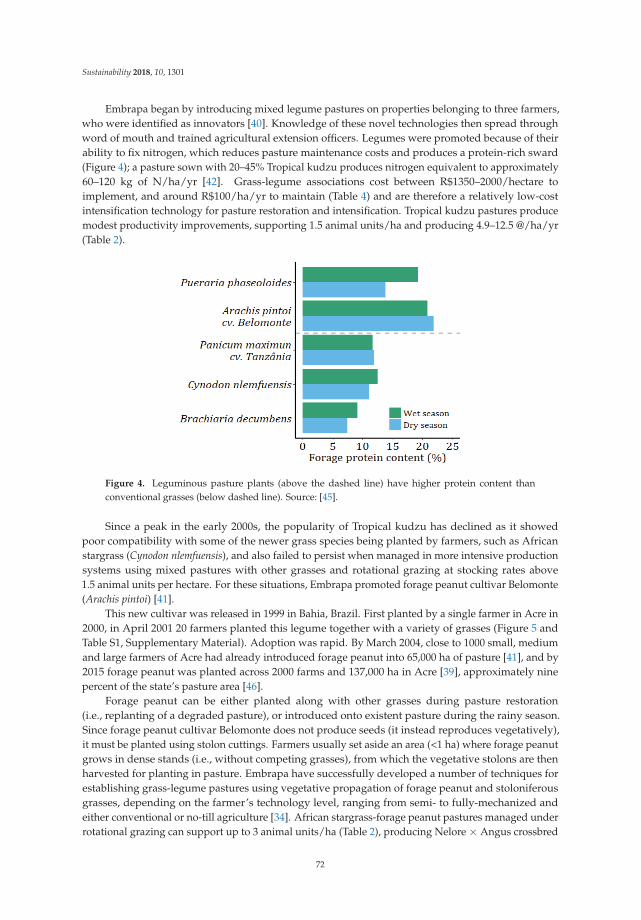
Sustainability 2018, 10, 1301
Embrapa began by introducing mixed legume pastures on properties belonging to three farmers,who were identified as innovators [40]. Knowledge of these novel technologies then spread throughword of mouth and trained agricultural extension officers. Legumes were promoted because of theirability to fix nitrogen, which reduces pasture maintenance costs and produces a protein-rich sward(Figure 4); a pasture sown with 20–45% Tropical kudzu produces nitrogen equivalent to approximately60–120 kg of N/ha/yr [42]. Grass-legume associations cost between R$1350–2000/hectare toimplement, and around R$100/ha/yr to maintain (Table 4) and are therefore a relatively low-costintensification technology for pasture restoration and intensification. Tropical kudzu pastures producemodest productivity improvements, supporting 1.5 animal units/ha and producing 4.9–12.5 @/ha/yr(Table 2).
Figure 4. Leguminous pasture plants (above the dashed line) have higher protein content thanconventional grasses (below dashed line). Source: [45].
Since a peak in the early 2000s, the popularity of Tropical kudzu has declined as it showedpoor compatibility with some of the newer grass species being planted by farmers, such as Africanstargrass (Cynodon nlemfuensis), and also failed to persist when managed in more intensive productionsystems using mixed pastures with other grasses and rotational grazing at stocking rates above1.5 animal units per hectare. For these situations, Embrapa promoted forage peanut cultivar Belomonte(Arachis pintoi) [41].
This new cultivar was released in 1999 in Bahia, Brazil. First planted by a single farmer in Acre in2000, in April 2001 20 farmers planted this legume together with a variety of grasses (Figure 5 andTable S1, Supplementary Material). Adoption was rapid. By March 2004, close to 1000 small, mediumand large farmers of Acre had already introduced forage peanut into 65,000 ha of pasture [41], and by2015 forage peanut was planted across 2000 farms and 137,000 ha in Acre [39], approximately ninepercent of the state’s pasture area [46].
Forage peanut can be either planted along with other grasses during pasture restoration(i.e., replanting of a degraded pasture), or introduced onto existent pasture during the rainy season.Since forage peanut cultivar Belomonte does not produce seeds (it instead reproduces vegetatively),it must be planted using stolon cuttings. Farmers usually set aside an area (<1 ha) where forage peanutgrows in dense stands (i.e., without competing grasses), from which the vegetative stolons are thenharvested for planting in pasture. Embrapa have successfully developed a number of techniques forestablishing grass-legume pastures using vegetative propagation of forage peanut and stoloniferousgrasses, depending on the farmer’s technology level, ranging from semi- to fully-mechanized andeither conventional or no-till agriculture [34]. African stargrass-forage peanut pastures managed underrotational grazing can support up to 3 animal units/ha (Table 2), producing Nelore × Angus crossbred
72

Sustainability 2018, 10, 1301
steers ready for slaughter within 24 months (Table S2, Supplementary Material), compared with the36+ months typical of extensive systems [41]. These productivity improvements also improve thefarm bottom line, increasing profitability from around R$41.10/ha/yr in traditional systems up toR$381.28/ha/yr (Table 2).
Figure 5. Nelore cattle (Bos indicus) grazing mixed pasture: forage peanut (Arachis pintoi cv.Belomonte) (the yellow flowering plants) with Brachiara spp.
Grass-legume pastures can mitigate greenhouse gas emissions by substituting for fossil-fueldependent nitrogen fertilizers, by reducing cattle slaughter ages [42,47], and by increasing soil carbonsequestration [48]. Additionally, Costa et al. [49] reported that mixed pastures of Brachiaria humidicola andforage peanut cv. Mandobi in Acre had 24% lower N2O emission (2.38 kg N ha−1 yr−1) than pure pastureof the same grass (3.13 kg N ha−1 yr−1) and similar emissions to native forest (2.47 kg N ha−1 yr−1).
3.2. Beef Case Study #2—Novo Campo Program
The Novo Campo Program (“New Field” Program in English) has involved 23 farms in the AltaFloresta region of Mato Grosso since 2012. Led by the Instituto Centro de Vida (ICV), with collaborationwith stakeholders from across the cattle supply chain (see Table 4 for a complete list of participatingorganizations), cattle productivity has been increased through a package of farm management changes.These include the introduction of pasture rotation, the adoption of so called “good agriculturalpractices” (GAP), correction of soil imbalances (e.g., by liming), pasture fertilization, and improvedfarm record keeping. The GAP is a voluntary set of “gold-standard” guidelines for sustainableproduction adopted across Brazil, which includes a check-list of 125 points of guidance across 11 areasof farm management, spanning farm economic management, social and environmental responsibilities,to pasture and herd management [50].
Together, these interventions have improved farm productivity and profitability, and reducedgreenhouse gas emissions (Figure 6). Beef production per hectare has increased from ~4.7 (the regionalaverage) to 7–24 @/ha/yr, which has reduced the cost of production per arroba on intensified farms byone third (R$66.33/@ vs. R$95.80/@) [38]. Profit increased from less than R$100/ha/yr to more thanR$600/ha/yr of pasture (Table 2). These yield-raising technologies require an initial investment ofR$1500–4000/ha, depending on the initial pasture condition, though these up-front costs are paid offafter an average of 2.5 years (Table 2).
73

Sustainability 2018, 10, 1301
Ta
ble
3.
Prod
ucti
vity
ofda
iry
inte
nsifi
cati
onin
itia
tive
ssu
rvey
ed.R
ange
sar
elis
ted
inbr
acke
ts,w
here
prov
ided
.
Nam
eo
fIn
itia
tiv
e
Base
lin
eS
tock
ing
Rate
(AU
/ha)
Sto
ckin
gR
ate
(AU
/ha)
Incr
ease
inS
tock
ing
Rate
ov
er
Base
lin
e
Base
lin
eP
rod
uct
ivit
y(L
/ha/y
r)
Pro
du
ctiv
ity
(L/h
a/y
r)
Incr
ease
inP
rod
uct
ivit
yO
ver
Base
lin
e
Base
lin
eP
rod
uct
ivit
y(L
/co
w/y
r)
Pro
du
ctiv
ity
(L/c
ow
/yr)
Incr
ease
inP
rod
uct
ivit
yo
ver
Base
lin
e
Years
toB
reak
Ev
en
on
Inv
est
men
t
Years
toA
chie
ve
Max
Pro
du
ctiv
ity
Ty
pic
al
pro
fit/
ha/y
r(R
$)
Silv
opas
tora
lSys
tem
wit
hR
otat
iona
lG
razi
ngfo
rD
airy
0.75
(0.5
–1.0
8)3.
5(2
.4–6
.3)
4.7x
~119
257
94(2
969–
9037
)4.
9x15
51(7
60–1
825)
1954
(164
2–24
82)
1.26
x2.
6(1
.8–6
.8)
6(5
–7)
4425
(217
6–80
92)
Flor
esta
sde
Val
or1.
1(0
.9–1
.2)*
3.1
(2.5
–3.7
)2.
8xD
ata
not
prov
ided
~319
0D
ata
not
prov
ided
~760
~110
01.
4x4
(3–5
)3
(2–4
)D
ata
not
prov
ided
*pr
oduc
tivity
data
are
nota
vaila
ble
from
part
icip
atin
gfa
rms
pre-
adop
tion,
and
soth
eba
selin
eda
taar
ees
timat
esof
the
regi
onal
aver
age
prod
uctiv
ityw
ithou
tthe
adop
ted
tech
nolo
gy.
Ta
ble
4.
Typi
calc
osts
invo
lved
inea
chin
tens
ifica
tion
initi
ativ
e.D
egra
ded
past
ures
are
past
ures
with
decl
inin
gpa
stur
efe
rtili
ty;t
heir
rest
orat
ion
ofte
nre
quir
esso
ilco
rrec
tion
,plo
ughi
ng,a
ndre
seed
ing
ofgr
asse
s,w
here
asso
ilco
rrec
tion
and
plou
ghin
gm
ayno
tbe
requ
ired
for
conv
enti
onal
past
ure
impr
ovem
ent.
Ran
ges
are
liste
din
brac
kets
,whe
repr
ovid
ed.
Nam
eo
fIn
itia
tiv
eO
rgan
izati
on
sIn
vo
lved
Ran
chin
gS
yst
em
s
Co
sto
fIn
ten
sifi
cati
on
(R$/h
a)
Co
sto
fP
ast
ure
Main
ten
an
ce(R
$/h
a/y
r)
Co
sto
fT
ech
nic
al
Ass
ista
nce
(R$/p
rop
ert
y/y
r)
Imp
rov
em
en
to
fD
eg
rad
ed
Past
ure
Imp
rov
em
en
to
fC
on
ven
tio
nal
Past
ure
Inte
nsifi
cati
onof
beef
catt
lepr
oduc
tion
syst
ems
wit
hth
eus
eof
mix
edgr
ass-
legu
me
past
ures
inA
cre
Embr
apa
Acr
e,Fe
dera
ção
deA
gric
ultu
rado
Esta
dodo
Acr
eFun
dode
Des
envo
lvim
ento
daPe
cuár
iado
Esta
dodo
Acr
e,&
Ass
ocia
ção
para
oFo
men
toà
Pesq
uisa
deM
elho
ram
ento
deFo
rrag
eira
s
Cow
-cal
f,ca
lfra
isin
g&
fatt
enin
g,fu
llcy
cle
Sem
i-m
echa
nize
dco
nven
tion
alpl
anti
ng:2
011.
Mec
hani
zed
conv
enti
onal
plan
ting
:14
61–1
920.
Mec
hani
zed
no-t
illpl
anti
ng:
1347
–180
6
~100
Dat
ano
tco
llect
ed
Nov
oC
ampo
Prog
ram
ICV,
Inte
rnat
iona
lIns
titu
tefo
rSu
stai
nabi
lity
(IIS
),Em
brap
a,So
lidar
ieda
d,Si
ndic
atos
Rur
ais
deA
lta
Flor
esta
eC
otri
guaç
u,JB
S,M
cDon
alds
,Arc
osD
oura
dos,
IMA
FLO
RA
,Alt
helia
Ecos
pher
e,Te
rras
,G
TPS,
Fund
oV
ale,
Nor
ad,&
the
Moo
reFo
unda
tion
Cal
frai
sing
&fa
tten
ing
3500
(300
0–40
00)
2000
(150
0–20
00)
1800
(150
0–20
00)
8000
(600
0–12
000)
Do
Cam
poà
Mes
aTN
C,M
arfr
ig,W
alm
art,
GTP
S,&
the
Moo
refo
unda
tion
Cal
frai
sing
&fa
tten
ing
1890
(175
0–18
97)
1468
(131
8–15
71)
~680
Dat
ano
tco
llect
ed
Silv
opas
tora
lSys
tem
wit
hR
otat
iona
lGra
zing
for
Beef
Ides
am,C
entr
opa
raIn
vest
igac
ión
enSi
stem
asSo
sten
ible
sde
Prod
ucci
ónA
grop
ecuá
ria
(CIP
AV
),V
iaVe
rde
Con
sulto
ria
Agr
opec
uári
a,Fu
ndo
Val
e,&
Viv
eiro
Sant
aLu
zia
Cow
-cal
f,ca
lfra
isin
g&
fatt
enin
g26
66(2
412–
3021
)A
llfa
rms
had
degr
aded
past
ure
~216
.25
~548
0
Silv
opas
tora
lSys
tem
wit
hR
otat
iona
lGra
zing
for
Dai
ryId
esam
,CIP
AV,
&V
iaVe
rde
Con
sult
oria
Agr
opec
uári
a,Fu
ndo
Val
e,&
Viv
eiro
Sant
aLu
zia
Cow
-cal
f53
55(4
900–
6866
)A
llfa
rms
had
degr
aded
past
ure
~275
~548
0
Flor
esta
sde
Val
or
IMA
FLO
RA
,CA
MPP
AX
(Coo
pera
tiva
Alt
erna
tiva
Mis
tado
Alt
oX
ingu
),A
DA
FAX
(Ass
ocia
ção
Des
envo
lvim
ento
daA
gric
ultu
raFa
mili
ardo
Alt
oX
ingu
),C
FA(C
asa
Fam
iliar
Rur
alde
São
Felix
doX
ingu
),Pe
trob
ras,
Fund
oV
ale,
&Fu
ndo
Am
azôn
ia
Cow
-cal
f~2
500
All
farm
sha
dde
grad
edpa
stur
e20
00(1
200–
2560
)25
00(2
000–
3000
)
74

Sustainability 2018, 10, 1301
By improving animal growth rates and so achieving slaughter weight in fewer days, farmersreduce emissions from enteric fermentation across the animal’s lifetime (enteric fermentationcontributes 67–83% of emissions, excluding land use change—a topic we return to in Section 4 [8,51,52]).This is seen from the experience on Novo Campo Program farms. Emissions have been reduced by36–59% (Figure 6), in large part through reductions in slaughter age down to 20–24 months (Table S2,Supplementary Material).
Figure 6. Two estimates for the emissions per kilogram of beef of conventional ranches and NovoCampo Program farms. Piatto and Costa Junior [53] compare emissions on pilot farms beforepasture intensification (baseline), with emissions after two years of participating in the initiative.Bogaerts et al. [8] compare farms participating in the Novo Campo Program with neighboringnon-participating farms. While both studies include emissions from enteric fermentation, manuremanagement, pasture fertilization, and fossil fuels required for pasture restoration, Bogaerts et al.also include emissions from concentrate feed production, and Piatto and Costa Junior include carbonsequestration in improved pasture and soil carbon emissions from degraded pasture. No emissionsfrom land use change are included, because no recent deforestation occurred on sampled farms.
Key changes in farm management are improved book-keeping and the introduction of rotationalpasture management. Adequate book-keeping is fundamental to understanding and improving farmmanagement processes, and yet is not done by a majority of farm managers or owners [4]. Farmers aretherefore trained in the importance of recording the costs of all inputs and the quantity and value ofbeef produced, to allow the calculation of the income and profit per arroba of beef. Once the economicperformance of the farm is established, rotational grazing is introduced.
Typically, 10–30% of the farms’ pasture area is fenced off into ca. 5-hectare plots, which aretargeted for pasture improvement. Pasture restoration begins with soil analysis to identify soilimbalances (e.g., pH). The pasture is then ploughed and limed (typically with 1500 kg/ha lime; Table S3,Supplementary Material), and the pasture is fertilized (400 kg/ha) and replanted, with Panicummaximun cv. Mombaça or Panicum maximun cv. Tanzânia grasses (Figure 7).
These fertilized plots have much higher productivity than conventionally managed pasture;in the first two years of the project, they produced 20.75 @/ha/yr compared with 10.75 @/ha/yracross the farm as a whole (Marcuzzo and de Lima, 2015). Cattle are moved through each fenced plotsequentially; the stocking rate and exact timing of the cattle rotation are based on the season, forageheight, and planted species, manipulated to maximize cattle growth while maintaining pasture fertility.With Panicum maximun cv. Mombaça, cattle enter plots when the grass height is around 90 cm andare moved when it has been grazed down to around 40 cm (approximately every five days in the wetseason, and less frequently during the dry season).
75

Sustainability 2018, 10, 1301
Figure 7. (a) High-yielding cattle pasture (right) on a Novo Campo Program farm, one month afterreplanting, compared with conventional, unreformed pasture (left); (b) Stocking rate in intensifiedpasture plots for the period January 2013–September 2014. The grey dashed line represents the meanstocking rate for farms in the region. Adapted from: [38].
While forage is in abundant supply in the rainy season (from approximately December–May), in thedry period, stocking rates in the intensified pasture areas are reduced (Figure 7), and supplementaryfeeding is necessary. Novo Campo Program farms have adopted a semi-feedlot feeding approach,where cattle are given supplementary concentrate feed in troughs in a confined area of pasture.One farm has also integrated soy and beef production to boost dry season feed availability. Soy isplanted on 200 ha, which is seeded with Brachiaria spp. after the soy harvest. This additional pasturearea then serves as an additional forage source during the dry period.
All Novo Campo participating farmers qualify for the GAP certificate, developed by Embrapa.The adoption of GAP requires training of farm personnel, and ultimately, approximately a 50% increasein on-farm labor. To support the dissemination of knowledge to staff on Novo Campo farms andbeyond, ICV therefore linked up with a local university, UNEMAT Alta Floresta, to train an additional40 agricultural extension officers in GAP, environmental licensing, farm financial analysis, and the useof farm management software [38].
Farms participating in the Novo Campo Program must also comply with Brazilian National LawNo. 12.651, the so called ‘Forest Code’. They must be registered in the rural environmental registry(Portuguese acronym CAR), cannot be blacklisted by the environmental police (IBAMA), and musthave had no illegal deforestation post-2008. On joining the Novo Campo Program, many farms haddegraded riparian areas, which legally must be reforested within 20 years. Properties received supportfrom ICV in restoring these areas, with the restoration actions depending on the degradation statusand location of streams. Where streams had some secondary regrowth and/or nearby forest, this mightinclude only fencing-off streams from cattle to foster natural regeneration; where riparian areas weremore degraded or isolated, they may have required direct seeding of trees, removal of grasses and thecontrol of pests. In both cases, restoration is not cheap with costs varying from R$2360/ha for passiverestoration, to R$9654/ha for active replanting [54].
76

Sustainability 2018, 10, 1301
To scale-up the results achieved in the Novo Campo Program, a commercial spin-off, PECSA,was launched in 2015. While management of the Novo Campo continues under ICV, PECSA appliesthe same package of technologies, in some cases intensifying more than the 30% of pasture area usedin the Novo Campo Program to increase farm productivity 3–5 times above the regional average [55].
3.3. Beef Case Study #3 Do Campo à Mesa
Launched in 2013, as a collaboration between The Nature Conservancy (TNC) and several partnersalong the beef supply chain (Table 4), the do Campo à Mesa initiative (“From Field to Table” in English)operates on 13 farms in São Félix do Xingu, Pará, to boost productivity through the establishment ofrotational pasture and training in GAP. Results after one year of the project are promising; stockingrates increased 20% and beef productivity 30% (Table 2), with substantially greater gains expected;beef productivity is forecast to increase more than 3.5-times to 17@/ha (10–27@/ha) within 12 years ofthe start of the project [37].
On joining the initiative, baseline data were collected by agricultural extension officers on theherd structure (e.g., number of animals, category, age, weight), farm operating costs, and soil condition.These are complemented with remote sensing analyses of the farm’s land use. Many farms hadconsiderable areas of degraded pasture, 23% and 18% of pasture was moderately or highly-degraded,respectively [37]. To combat this, management plans were drawn up to improve 20% of the farm’spasture area each year so that after five years all pasture would be in improved condition.
Goals for stocking rates were set, aiming to gradually increase stocking rates from 0.87 AU/hato 3.0 AU/ha. To achieve this, the initiative has used pasture improvement (weeding and liming,and resowing of pasture if degraded), education of farm workers in GAP, and the establishment ofrotational grazing. Livestock are also given 1.5 kg/head/day of protein supplementary feed in the dryseason, to overcome the seasonal deficit in feed availability.
The main costs of improving farming practices come in three forms: pasture improvement andmaintenance, adoption of GAP, and costs of environmental compliance; these costs vary strongly withfarm size. Pasture improvement requires an initial investment of between R$1300–1900/ha/yr (Table 4),and adoption of GAP requires not only worker education, but also improvements in infrastructureand more farm labor. After 12 years of the project, the requirement for labor is forecast to increase onaverage 54%, with larger increases on the biggest farms [37]. On small farms labor is family-basedand will be kept constant, while large farms plan to increase their number of employees three-fold.Do Campo à Mesa farms must also be compliant with the Forest Code, which also incurs substantialcosts. Compulsory restoration of deforested areas added an extra 30–250% to the cost of adoptingimproved farm practices [37]. Taking all the costs of the transition to more sustainable farming practicestogether, pasture intensification and legal compliance generated better economic returns for largefarms (>500 ha of pasture) ([37]. Costs per hectare for the three smallest properties were on average2.3 times higher than for other farms, and the two smallest farms, with 44 and 126 ha of pasture area,were not projected to make a profit and subsequently elected not to continue with cattle intensification.To help overcome the initial cost barrier and support the growth of the program, TNC helps farmersapply for loans from the Brazilian government’s low carbon fund (the “Plano ABC”, in Portuguese).
3.4. Beef Case Study #4—Silvopastoral System with Rotational Grazing for Beef
In 2011, the Institute for Conservation and Sustainable Development of the Amazon (Portugueseacronym, Idesam) launched the Silvopastoral System with Rotational Grazing initiative (“SistemaSilvipastoril com Pastejo Rotacional”, in Portuguese), on beef and dairy farms in Apuí, Amazonas.The initiative is working with 10 beef farms to boost productivity of smallholder beef production(results for dairy farms are listed in diary case study #1). While the planting of trees and shrubs,involves high up-front costs (Table 4), participating beef farms have improved productivity from4–7@/ha/yr to 12–20@/ha/yr, and profitability from ~R$130/ha/yr to R$260/ha/yr (Table 2).
77

Sustainability 2018, 10, 1301
Farm improvement begins with a visit from an agricultural extension technician, collectingbaseline farm information and drawing up management plans with the farmer. To introducerotational grazing, an area of between 20–50 hectares is intensified on each farm by restoring pasturethrough the application of lime, where required. This area is then divided into six plots, sown withPanicum maximum cv. Mombaça or Brachiaria brizantha, fertilized with phosphorus, and managed in arotational system. Cattle are moved through each plot approximately every 6–7 days according to thepasture condition.
These plots are divided by double electric fences (1.5 to 2 m in width) protecting a line of treesplanted 3 m apart (Figure 8). The trees are mostly native species, half of which are planted for theirtimber or other economic value and the other half are a mix of leguminous tree species (20–30 trees/ha),including Inga-de-metro (Inga edulis Mart.) Leucaena (Leucaena leucocephala var. cunningham) Paricá(Schizolobium amazonicum) Gliricídia (Gliricidia sepium), Jatobá (Hymenaea courbaril), and Parkia spp.Among the trees, fodder shrubs are also planted, including Tithonia diversifolia and Cratília (Cratyliaargentea). The principal benefits of planting leguminous trees and fodder shrubs in pasture are thatthe leaves provide a high-protein feed [56], increased shade which can reduce heat stress in cattle [57],and nitrogen-fixation which boosts grass growth and can improve soil condition [58].
Figure 8. (a) Producer standing with a tree line of 4-month old leguminous trees in an Idesamsilvopastoral system; (b) silvopastoral system once the bushes and trees are 2 years old.
Silvopastoral systems do, however, require careful management and substantial initial investment.Trees need protection from heavy grazing for the first 12–24 months post-planting; thereafter theyrequire occasional pruning if they get too broad in order to avoid excessive shade hindering grassgrowth [59]. Farmers must also closely monitor herd performance, including daily recording ofstocking rates. These changes require on average a 20% increase in on-farm labor. Farmers aresupported throughout the process by monthly visits from Idesam’s agricultural extension staff.Costs of implementing silvopastoral systems are high, R$2400–3020/ha, though this is offset bylow maintenance costs around R$220/ha/yr, in part because leguminous pastures do not require anynitrogen fertilizer application.
While it is hoped that productivity increases will reduce greenhouse gas emissions on participatingfarms, a recent analysis found that participating farms had higher greenhouse gas emissions thanneighboring farms (47 vs. 40 kg CO2e/kg beef) [8]. These results should, however, be treated withcaution as the analysis used the Cool Farm Tool, an out-of-the-box greenhouse gas calculator whichis not tailored for measuring emissions from integrated systems, and the input data were collectedless than one year after the program’s implementation. The environmental and economic impacts ofintegrated systems, such as silvopastoral systems, are difficult to model because the different parts ofthe management system interact [60], in this case, leguminous trees fertilize the pasture, supportinggrass growth. The Cool Farm Tool, though comprehensive in many respects, does not consider theseinteractions, simplifying the farm’s environmental footprint and potentially over-estimating emissions.
78

Sustainability 2018, 10, 1301
Similarly, while the Cool Farm Tool can calculate carbon sequestered in trees on-farm, this sourceof sequestration was not included in Bogaerts et al. [8]. Additionally, the farm-level data used werecollected shortly after the implementation of rotational grazing, therefore, emissions associated withpasture improvement were counted before productivity gains had been realized. As it is expected totake five years for the systems to achieve full productivity (Table 2), using data from only the first yearoverestimates emissions from participating farms.
Finally, to participate in the initiative, farms must also be compliant with environmental legislation.They must be registered on the CAR, develop a PRAD (the “Projeto de Recomposição de ÁreasDegradadas e/ou Alteradas”, a plan for restoration if the property does not meet minimum legalrequirements for forest cover), and agree to not clear any new areas of forest.
3.5. Dairy Case Study #1—Silvopastoral System with Rotational Grazing for Dairy
Idesam also work with 11 smallholder pilot farms (ranging from 83–340 ha in size; Table 1) inthe state of Amazonas, to increase dairy productivity through the rotational management of pasturelined with timber and leguminous trees, and shrubs. As for Idesam’s beef intensification in the region,the dairy initiative has seen productivity improvements, a 1.26-fold increase in milk production percow and 4.9-fold increase in milk production per hectare (Table 3).
Plots of intensively managed pasture are divided by doubled electric fences protecting a lineof trees and shrubs. Compared with Idesam’s beef system, the dairy farms use a greater number ofplots (~40) and trees (50 to 110/ha). Around 6 hectares is targeted for intensive management on eachfarm, with 0.1 to 0.9 hectares per plot. Forty-four percent of the tree species were planted to provideshade for cattle and timber as a source of long-term income for farmers; 56% were leguminous [61].As often required in the region, the soil was supplemented with lime, before planting Brachiariabrizantha, Panicum maximum cv. BRS zuri or cv. Massai grasses, with phosphorus added as necessary.These grasses show high productivity in the shady conditions typical of silvopastoral systems [57,62].Laboratory experiments have shown, for example, that shade can even increase the protein content ofPanicum maximum grasses [63].
The system is managed in rotation, where cattle are moved through plots every 12 h to two days,depending on grass height. In the drier months, the deep-rooted leguminous trees continue to providea source of fodder, and some farmers supplement feed with maize silage or “cut-and-carry” feeding ofTithonia diversifolia, Inga edulis, and Cratylia argentea. Lactating cattle on some farms also receive 1.5 kgof maize-based concentrate feed at milking each day. Water availability is crucial for high-productivitydairy production, and so drinking water is pumped into elevated water boxes, which distribute it bygravity through a system of buried hoses to each pasture plot (Figure 9).
Figure 9. (a) Installation of underground piping to deliver water to each plot in the SilvopastoralSystem with Rotational Grazing for Dairy initiative; (b) Dairy cattle drinking from one of the watertroughs, with electric fencing in the foreground.
79

Sustainability 2018, 10, 1301
Systems with leguminous trees require approximately 15% more labor than conventionalpasture-based systems. The trees require protection from grazing and insects for the first few months,as well as intermittent pruning during the first three years. The requirement for tree care reduces as thetrees mature, and the rotational management of cattle in these systems requires no additional specificmanagement, as cattle are moved twice a day for milking in any case.
The implementation of leguminous systems can be costly, ranging from R$4900–6900/ha to coverthe costs of pasture reformation, tree planting, electric fencing (for managing rotational grazing),and construction of water sources in each plot (Table S3, Supplementary Material). Though theseinitial costs are paid off within 2–7 years (Table 3), as improved management boosts profitability fromR$1281.15/ha/yr to around R$4425/ha/yr, Idesam has provided financial support to the first farmersof the program. Farmers paid 20% of the cost of implementation, with Idesam covering the remaining80%. To access this financial support and participate in the initiative, farmers must commit to legalcompliance with the Forest Code. Farms must be registered in the CAR, commit to not deforest further,and restore non-forested areas and degraded riparian strips, in line with the PRAD.
3.6. Dairy Case Study #2—Florestas de Valor
The dairy intensification project Florestas de Valor (“Forests of Value” in English) was launchedby the Institute of Forestry and Agricultural Management and Certification (Portuguese acronym,IMAFLORA) in 2015, and operates on six farms in São Félix do Xingu in the state of Pará.By concentrating production on a small, intensively managed portion of pasture in each farm, they haveincreased stocking rates almost three-times above the regional average, with 85% higher productivityper cow (3240 L milk/cow/yr vs. 1750 L/cow/yr; Table 3).
Florestas de Valor operates on small properties, ranging from 25–200 hectares in size (Table 1).These farms rely almost entirely on family labor, and so it is important that the intensification does notincrease the overall requirement for labor. This is achieved by focusing production on a small area ineach farm, where 3.5–11 hectares are selected for intensification and divided into 10–15 fenced plots(Figure 10). The soil in each plot is analyzed before soil correction, and either direct resowing withBrachiaria brizantha MG5, Panicum maximum cv. Mombaça, Brachiaria decumbens or Panicum maximumcv. Massai, or pasture restoration through crop-livestock integration. On four properties, maizewas planted on degraded pasture; once the maize was harvested, pasture grasses were then sown.The fences between pasture plots are planted with leguminous trees, including Canavalia ensiformis,Inga edulis and Cajanus cajan. Trees were planted three meters apart, with an average of 66 trees perhectare. Cattle remain approximately three days in each plot, thereby completing a cycle of eachplot every 30–45 days. In the dry season, when grass growth is slower and over-grazing is morelikely, less time is spent in the fenced plots, and cattle are instead put onto pasture that has beenintentionally rested.
Overall, it costs around R$2500/ha to implement the rotational grazing and leguminous treesystems. These costs stem from costs of soil improvement, grass seeds, maize planting, fencing,solar panels, and in-pasture water sources (Table S3, Supplementary Material). Of the 50 hectaresintensified, IMAFLORA funded 36 hectares, with farmers covering the costs of the remaining14 hectares. In either case, because of improvements in productivity, the total initial cost is expected tobe paid off within 3–5 years.
80

Sustainability 2018, 10, 1301
Figure 10. Around 10% of each property in the Florestas de Valor initiative is divided into small plotsusing fences lined with leguminous trees (yellow lines in the main image). Top right: intensified pasturearea shown within the total farm boundary (black line). Lower right: The farm location is shownas a point within Sao Felix do Xingu (municipality colored in blue). State abbreviations: PA = Pará,MT = Mato Grosso, TO = Tocantins.
4. Discussion
The results from these initiatives suggest that there are a variety of available technologies that canincrease cattle ranching productivity and profitability in the Amazon. Though diverse in the details,these initiatives share many similarities, including their focus on farmer training, farm record-keeping,and improved pasture management, in particular, the adoption of rotational grazing and pasturefertilization using chemical inputs or leguminous plants. These management changes require someinitial investment (R$1300–6900/hectare), which is paid off within 2.5–8.5 years.
With the exception of the introduction of grass-legume pastures in Acre, the initiatives presentedare young and further productivity gains are expected, with productivity expected to peak 1.5–7 yearsafter implementation (Tables 2 and 3). Our study is, however, not a large-scale randomized controlledtrial, and so these promising results come with a number of caveats. First, we do not claim thatour review is exhaustive, though we present results from six of the thirteen initiatives that weare aware of which operate in the region (Table S4, Supplementary Material), and we believe ourresults are broadly representative of high-yielding cattle ranching in the Amazon. Second, theseinitiatives recruited farmers opportunistically, predominantly through farmer networks and openfarm days (Figure 11). The farmers participating are therefore “early-adopters”, who may differfrom other farmers in systematic ways, for example by being less risk averse. We do not believethat the productivity gains that we observe result from these farmer differences or fundamentaldifferences between these farms and their neighbors. For three of our six initiatives, we presentproductivity estimates from before and after the interventions showing clear productivity increases(for the other three, the Novo Campo Program, Florestas de Valor and mixed legume pastures in Acre,pre-intervention data were not available and our baseline data are estimates of the regional averageproductivity; Tables 2 and 3). Our data are also self-reported, though our productivity improvementsare in line with previous literature on the productivity gains from improvements in farm managementin Brazil [5,64–67], and our estimates of the costs of intensification are an important resource foraccurately estimating the cost-effectiveness of cattle intensification in the Amazon. Previous work on
81

Sustainability 2018, 10, 1301
the cost of cattle intensification has typically focused only on direct costs of pasture improvement,thereby underestimating the true cost of intensification for farmers. When modelling the pastureimprovement included in Brazil’s contribution to the UNFCC, De Oliveira Silva et al. [5], for example,estimate costs between R$365–1243/ha and maintenance costs from R$6.9–266.8/ha, estimates whichare substantially lower than our figures. Their figures, however, do not include indirect costs such ascosts from the transportation of inputs, increased labor, or costs from fencing and the implementationof rotational grazing.
Figure 11. Relative importance (1 = least important, 6 = most important) of six different channelsfor recruiting farmers into the six initiatives described in this article. All initiatives recruitedfarmers opportunistically, as knowledge about the initiatives was spread for the most part throughword-of-mouth, field days where neighboring farmers were invited to tour participating farms, and thetraining of rural extension officers in GAP. Idesam’s beef and dairy initiatives took similar approachesto recruitment, and so the results are grouped for these two initiatives.
4.1. Risks of Cattle Intensification
Whatever the financial costs, increasing cattle ranching yields in the Amazon is not withoutrisks [68]. Improving productivity can reduce greenhouse gas emissions from beef production, as seenboth at the farm-scale in the Novo Campo Program (Figure 6) and other intensification initiativesin the region [8], and at the national-scale from coupled economic-environmental modelling [6].Cohn et al. [6] find that the adoption of GAP in Brazil could halve greenhouse gas emissions fromdeforestation and agriculture, though in practice the land sparing effect of cattle productivityincreases are likely to vary spatially. While in consolidated regions, economic theory suggests thatintensification can help reduce deforestation through market and labor effects [69,70], in forestedregions intensification risks rebound effects—the so-called “Jevon’s paradox” where increases in theprofitability of cattle ranching incentivize, rather than reduce, local deforestation. Reconciling targetsfor increased cattle production and zero illegal deforestation or even deforestation-free production willtherefore require explicitly linking improvements in cattle ranching with habitat protection and effortsto reduce leakage in cattle supply chains [71,72]. It is also with this rebound effect in mind that theinitiatives described in this article explicitly require participating farmers to comply with the Brazilian
82

Sustainability 2018, 10, 1301
Forest Code, have no recent illegal deforestation, and develop land use plans for reforestation whererequired. Further discussion of potential risks is included in the online Supplementary Material.
While the technologies discussed in this article can increase farm profitability, this is also notalways the case; results from two of our initiatives show that pasture intensification may, in somecases, be more profitable on large, rather than small farms. In the do Campo à Mesa initiative, pastureintensification was not profitable within twelve years for the two smallest farms, suggesting that thereis a tipping point in economic returns between 126 and 425 ha of pasture [37]. Similar economies ofscale were found in a modelling study using data from the Novo Campo Program (which found that theintroduction of GAP and rotational grazing intensification was only profitable on farms with >385 haof pasture; IIS, 2015), and in other studies of cattle ranching economics [4,73]. On the other hand,these economies of scale appear to be technology and system dependent. Positive economic returnswere seen for smallholder dairy producers, and silvopastoral beef systems in Apuí (Tables 2 and 3),which can turn a profit with as little as 20 hectares of pasture. Similarly, grass-legume pastureshave been adopted by small- and large-farms alike in Acre [41,74]. Given that 78% of cattle-rearingfarms (hosting 33% of cattle) in the Amazon biome have less than 200 hectares of pasture (Figure S2,Supplementary Material), it is important that efforts to improve profitability and farmer livelihoods inthe cattle sector include both large- and small- landholders.
4.2. Barriers to Scaling up Sustainable Cattle Ranching
Cattle production in Brazil is set to grow; the Brazilian government recently set ambitious targetsfor increasing beef and dairy production by 40% [75]. The sustainable growth of the industry is not,however, guaranteed. To ensure that the cattle industry develops sustainably, improving farmerlivelihoods while protecting the environment, will require a mix of the right financial incentives, effortsto support training of rural workers and agricultural extension services, and improved monitoring ofcattle supply chains.
Most cattle ranchers adopt good agricultural practices because of the expected improvements inproductivity and profitability [76]. However, implementation costs and difficulty in accessing creditare barriers for many producers. Among producers surveyed in Mato Grosso regarding adoptionof good agricultural practices, 18% cited financial constraints as a barrier to adoption [76], and highimplementation costs are also an important barrier for four of the six cattle initiatives described in thisarticle (Figure 12).
Figure 12. (a) The most important barriers to the implementation of sustainable cattle initiatives,and (b) the solutions to these barriers, as identified in the survey of the organizations running the sixsustainable cattle ranching initiatives described in this article.
83

Sustainability 2018, 10, 1301
Sustainable growth in the cattle industry must also combine productivity improvements with theprotection of native vegetation. In the Amazon biome, farmers are required to keep 80% of their landunder forest (the threshold is set at 50% for small properties and properties in Ecological and EconomicZoning areas), and must reforest any land deforested above this threshold, or purchase certificatesthrough the nascent forest trading scheme to compensate [77]. As the forest certificate market is notyet operating at scale, farmers currently rely on on-site reforestation for legal compliance, and the costscan be substantial. The do Campo à Mesa and Novo Campo Program initiatives report reforestationcosts of R$868–6068/ha and R$2360–9654/ha, respectively. These figures are roughly equivalent to thecosts of pasture intensification and implementation of GAP. Unfortunately, even where farmers canaccess credit, no credit lines currently support costs of compliance with the Forest Code [37].
The financial barriers to improved cattle production and compliance with the Forest Code can,however, be overcome by developing the right private and public incentives for producers (Figure 12).Currently, farmers receive the same price for their product, regardless of their environmentalmanagement. This could be fixed by the development of sustainable beef price premiums andcertification schemes, such as the “Standard for Sustainable Cattle Production Systems” developed bythe Sustainable Agricultural Network, which delivers a financial reward to producers implementinggood practices [78]. Similarly, agricultural credit can be leveraged for sustainability, by making accessto agricultural credit contingent on the adoption of sustainable ranching practices, and by supportingthe costs of meeting the requirements of the Forest Code.
As an example of sustainable credit, in 2010 Brazil created the landmark ABC Program, one ofthe world’s first credit lines for low carbon agriculture [79], which supports the costs of restoringdegraded pasture and the implementation of integrated crop-livestock-forestry systems. The impact ofthe ABC Program has, however, been hampered by bureaucratic issues, unfavorable interest rates, anda lack of public awareness. Producers perceive the ABC program as being complex, slow, and overlybureaucratic [76]—posing a particular problem for small producers [80]. The ABC Program is oftenout-competed by other credit lines; its interest rates (7.5–8% per year) are double that of loans availablethrough the National Rural Credit System, Brazil’s main source of agricultural credit [79]. Publicawareness is also a problem. Surveys in the Alta Floresta region of Mato Grosso show that mostproducers have not heard of the ABC Program and are not familiar with the concept of sustainablecredit lines [80]. Only 10% of the ABC Program’s budget is spent in the northern states, which makeup the majority of the Amazon biome [81]. Overall, sustainable credit lines make up only 1.9% ofall agricultural credit in Brazil [79], and there are currently no sustainable credit lines which arespecifically aimed at smallholders, though these could be created within the existing National Programfor Strengthening Family Agriculture (Portuguese acronym, PRONAF) [79].
The widespread adoption of sustainable cattle ranching will, of course, require more than justthe correct mix of financial incentives. Barriers are also posed by a shortage of trained labor, farmerrisk aversion, and the complexity of cattle supply chains. Improved farm performance cannot beachieved without the adequate training of farm staff. The lack of qualified labor is, however, acutein both beef and dairy production [76,82]. Sixty-five percent of ranchers surveyed in Alta Floresta,Mato Grosso, cited a shortage of qualified labor as the main barrier to the adoption of good agriculturalpractices [76]. Access to agricultural extension services is also limited [11]. Four-fifths of dairy farmersin Mato Grosso, for example, have never received technical assistance [28].
Farmer psychology also plays an important role (Figure 12). High-yielding cattle ranchingcosts more in the short term, though it generates positive returns in the longer-term (Tables 2 and 3).Many cattle ranchers are, however, risk averse [4] or not motivated by profit-maximization [83], and thetransition from low-input, low-risk extensive systems to intensive pasture management requires tosome degree a shift in mindset. Improved farm management begins with improved record-keeping,which is a foreign concept to most producers [4]. Rotational grazing systems also require that cattle aremoved more frequently. Nelore cattle breeds have a reputation as being difficult to handle, though thisis in large part because in extensive systems they are not used to contact with farm staff. While regular
84

Sustainability 2018, 10, 1301
contact with farm laborers does improve their temperament [84], farmers can at first take someconvincing about the feasibility of new management practices. The required shift in mindset is perhapseven greater for the adoption of silvopastoral systems and mixed grass-legume pastures. Farmersused to thinking of cattle as animals which graze grass may be initially reluctant to incorporate treesor herbaceous legumes (usually considered as undesirable species) into pasture as a source of forageand fertilizer.
These psychological barriers can perhaps be overcome by increasing familiarity with high-yieldingsystems, which remains low [80]. Awareness can be raised by establishing demonstration units on realfarms, as in the six initiatives described in this article, and open-farm field days so that local farmerscan witness and learn about new management options (Figure 11). As Brazilian farmers’ receive mostof their farming advice from other farmers [85], word-of-mouth dissemination of new technologiesis critical, and can be effective, as seen in the experiences of legume pastures in Acre. The existenceof local champions, long-term commitment of key players, and strategic partnerships among localstakeholders are also key to successful wide adoption of intensive cattle production systems [41].
Finally, there are structural barriers to sustainable cattle ranching. Cattle supply chains arecomplex, which means that deforestation is difficult to eradicate. While market initiatives (such asthe “Terms of Adjustment of Conduct” and “G4” agreements) require meatpacking companies toblock sales from properties with illegal deforestation (the G4 prohibits new deforestation altogether),this applies only to properties which supply cattle directly to slaughterhouses. As cattle may be bornon one ranch, reared on a second, and fattened on a third, leakage is widespread. Though theseagreements have reduced deforestation among the direct suppliers of slaughterhouses, it has notled to overall reductions in deforestation [71]. To permit growth of the Brazilian beef industry whilereducing deforestation will therefore require efforts to reduce leakage. This could be achieved either bymonitoring the movements of individual cattle, for example, using unique ear tags, or by monitoringfarm-to-farm movement of batches of cattle. This information is already collected as part of the Guideto Animal Transport (GTA) used to track animal sanitation and health, but it is not used for monitoringenvironmental compliance.
While the barriers to scaling-up high-yielding cattle ranching in the Amazon are numerous, thereis cause for optimism. First, cattle productivity is already increasing in most regions of Brazil [13,86].Second, the example of leguminous pasture adoption in Acre shows that local demonstration farmscan lead to technology diffusion at a regional scale in the Amazon. Third, though focused in southernBrazil, lessons can be learned from the dairy extension initiative, the Projeto Balde Cheio (“Full Bucket”project in English). The program began in 1999 in two municipalities in the states of São Pauloand Minas Gerais, where demonstration units were established on twelve farms. Operating on abudget of only R$5000–45,000 (US$5000–23,000) per year, agricultural extension officers from Embrapaworked with farmers to introduce a package of new practices, including improved farm book-keeping,soil conservation, pasture fertilization, and rotational management. On average, family farmerswho joined the program increased milk production three-fold [82], with higher productivity arisingfrom a combination of more lactating cows/area (31%), higher productivity/cow (24%), and betterlabor performance (37%), while using less land area (−7%). The initiative has since expanded, as thenumber of farmers assisted rose from 400 in 2010 to more than 3000 in 2012, and is now present in483 municipalities nationwide, including farms in Rondônia, Pará and Amazonas, within the Amazonbiome (Table S4, Supplementary Material).
5. Conclusions
As cattle ranching makes up the majority of agricultural land and productivity is still well belowits sustainable potential, improvements in cattle productivity are key to the sustainable intensificationof Brazilian agriculture. We present results from six cattle ranching initiatives which have achievedhigher productivity and profitability in the Brazilian Amazon, while also supporting compliance withthe Forest Code. These initiatives are, for the most part, still young and so we conclude by setting out
85

Sustainability 2018, 10, 1301
three key conditions which are required to mainstream sustainable cattle ranching in the Amazon.If these conditions are met, we believe that the Brazilian beef industry can profitably produce more onless land and thereby facilitate growth in the agricultural sector while protecting Brazil’s remainingnative vegetation.
(1) Large-scale knowledge transfer—long-term funding and support is required for farmer-centeredagricultural extension services, which increase awareness of high-yielding technologies andsupport small- and large-holders alike to adopt appropriate farming practices.
(2) Financial support for sustainable cattle ranching—farmers must be incentivized to adoptsustainable ranching practices, both through competitive, sustainable credit lines and throughmarket signals. Rural credit lines should include sustainability criteria, and should help farmersnot only increase agricultural production, but also meet the costs of Forest Code compliance.Market signals also matter, and just as some slaughterhouses offer price-premiums for high meatquality, price-premiums for GAP would encourage farmer uptake.
(3) Increase transparency in cattle supply chains—efforts by some slaughterhouses to monitor directsuppliers are a step in the right direction, but do not go far enough. All slaughterhouses shouldmonitor both indirect and direct cattle suppliers, and monitoring efforts should be independentlyaudited and publicly reported, so that deforestation may ultimately be eliminated from cattlesupply chains.
Supplementary Materials: The following are available online at http://www.mdpi.com/2071-1050/10/4/1301/s1,supplementary text about the risks of cattle intensification; Tables S1–S4, and Figures S1 and S2.
Acknowledgments: We thank Fabio Ramos, Daniel Silva, André Novo, Artur Camago, Abdias Machado,Kemel Kalif, Márcio Rangel, Ezequiel Rodrigues do Valle, Marcelo Stabile, Mariano Cenamo, João Pedro Pio,Toby Gardner, Ben Phalan, Javier Godar, Livia Matyucheva, Priscila da Cunha Lessa, and Jose Guerrero for theirinput at various stages of the project. Erasmus K.H.J. zu Ermgassen was funded by BBSRC grant BB/J014540/1and the Tim Whitmore Trust Fund. Funding for open access publishing come from BBSRC grant BB/J014540/1.
Author Contributions: Erasmus K.H.J. zu Ermgassen co-designed the study, wrote the survey, collected the data,analysed the data, and led on the writing of the manuscript. Bernardo B.N. Strassburg and Agnieszka Latawiecco-designed the study; Melquesedek Pereira de Alcântara, Francisco Beduschi Neto, Murilo M. F. Bettarello,Genivaldo de Brito, Gabriel C. Carrero, Eduardo de A.S. Florence, Edenise Garcia, Eduardo Trevisan Gonçalves,Casio Trajano da Luz, Giovanni M. Mallman, and Judson F. Valentim provided data, and all co-authors contributedsubstantially to the writing of the manuscript.
Conflicts of Interest: This manuscript reports the results of six initiatives which have increased the productivity ofcattle ranching in the Brazilian Amazon. Many of the authors (Melquesedek Pereira de Alcântara, Francisco BeduschiNeto, Murilo M.F. Bettarello., Genivaldo de Brito, Gabriel C. Carrero, Eduardo de A.S. Florence, Edenise Garcia,Eduardo Trevisan Gonçalves, Casio Trajano da Luz, Giovanni M. Mallman, Bernardo B.N. Strassburg, Judson F.Valentim, and Agnieszka Latawiec) were directly involved in the development of these initiatives. The foundingsponsors had no role in the design of the study; in the collection, analyses, or interpretation of data; in the writing ofthe manuscript, and in the decision to publish the results.
References
1. FIESP Outlook FIESP 2026: Projections for Brazilian Agribusiness; Federação das Indústrias do Estado de SãoPaulo: São Paulo, Brazil, 2016.
2. Brazil Intended Nationally Determined Contribution towards Achieving the Objective of the United NationsFramework Convention on Climate Change. Available online: http://www4.unfccc.int/submissions/INDC/Published%20Documents/Brazil/1/BRAZIL%20iNDC%20english%20FINAL.pdf (accessed on16 April 2018).
3. Strassburg, B.B.N.; Latawiec, A.E.; Barioni, L.G.; Nobre, C.A.; da Silva, V.P.; Valentim, J.F.; Vianna, M.;Assad, E.D. When enough should be enough: Improving the use of current agricultural lands could meetproduction demands and spare natural habitats in Brazil. Glob. Environ. Chang. 2014, 28, 84–97. [CrossRef]
4. Barbosa, F.A.; Soares Filho, B.S.; Merry, F.D.; de Oliveira Azevedo, H.; Costa, W.L.S.; Coe, M.T.; da SilveiraBatista, E.; Maciel, T.C.; Sheepers, L.C.; de Oliveira, A.R.; et al. Cenários para a Pecuária de corte Amazônica;Universidade Federal de Minas Gerais: Belo Horizonte, Brazil, 2015; p. 154.
86

Sustainability 2018, 10, 1301
5. De Oliveira Silva, R.; Barioni, L.G.; Queiroz Pellegrino, G.; Moran, D. The role of agricultural intensificationin Brazil’s Nationally Determined Contribution on emissions mitigation. Agric. Syst. 2018, 161, 102–112.[CrossRef]
6. Cohn, A.S.; Mosnier, A.; Havlik, P.; Valin, H.; Herrero, M.; Schmid, E.; O’Hare, M.; Obersteiner, M.Cattle ranching intensification in Brazil can reduce global greenhouse gas emissions by sparing land fromdeforestation. Proc. Natl. Acad. Sci. USA 2014. [CrossRef] [PubMed]
7. De Oliveira Silva, R.; Barioni, L.G.; Hall, J.A.J.; Moretti, A.C.; Fonseca Veloso, R.; Alexander, P.; Crespolini, M.;Moran, D. Sustainable intensification of Brazilian livestock production through optimized pasture restoration.Agric. Syst. 2017, 153, 201–211. [CrossRef]
8. Bogaerts, M.; Cirhigiri, L.; Robinson, I.; Rodkin, M.; Hajjar, R.; Costa Junior, C.; Newton, P. Climate changemitigation through intensified pasture management: Estimating greenhouse gas emissions on cattle farms inthe Brazilian Amazon. J. Clean. Prod. 2017, 162, 1539–1550. [CrossRef]
9. Piccoli, M.L.; Braccini Neto, J.; Brito, F.V.; Campos, L.T.; Bértoli, C.D.; Campos, G.S.; Cobuci, J.A.;McManus, C.M.; Barcellos, J.O.J.; Gama, L.T. Origins and genetic diversity of British cattle breeds in Brazilassessed by pedigree analyses. J. Anim. Sci. 2014, 92, 1920–1930. [CrossRef] [PubMed]
10. Townsend, C.R.; de Lucena Costa, N.; de Araújo Pereira, R.G. Aspectos Econômicos da Recuperação de Pastagensno Bioma Amazônia; EMBRAPA: Porto Velho, Brazil, 2009; p. 28.
11. Valentim, J.F. Desafios e estratégias para recuperação de pastagens degradadas e intensificação da pecuáriaa pasto na Amazônia Legal. In Simpósio de Pecuária Integrada; Pereira, D.H., Carneiro e Pedreira, B., Eds.;Recuperação de Pastagens: Anais; Fundação Uniselva: Cuiabá, Brazil, 2016; pp. 11–56.
12. Dias-Filho, M.B.; Andrade, C.M.S. De Pastagens no Trópico Úmido; Embrapa Amazônia Oriental: Belém, Brazil,2006; p. 33.
13. Dias, L.C.P.; Pimenta, F.M.; Santos, A.B.; Costa, M.H.; Ladle, R.J. Patterns of land use, extensification, andintensification of Brazilian agriculture. Glob. Chang. Biol. 2016, 22, 2887–2903. [CrossRef] [PubMed]
14. Bowman, M.S.; Soares-Filho, B.S.; Merry, F.D.; Nepstad, D.C.; Rodrigues, H.; Almeida, O.T. Persistenceof cattle ranching in the Brazilian Amazon: A spatial analysis of the rationale for beef production.Land Use Policy 2012, 29, 558–568. [CrossRef]
15. Ministério da Agricultura, Pecuária e Abastecimento; Ministério da Ciência, Tecnologia, Inovações eComunicações; Ministério do Meio Ambiente. Projeto Terraclass 2012; Embrapa & INPE: Brasília, Brazil, 2014.
16. Börner, J.; Kis-Katos, K.; Hargrave, J.; König, K. Post-Crackdown Effectiveness of Field-Based Forest LawEnforcement in the Brazilian Amazon. PLoS ONE 2015, 10, e0121544. [CrossRef] [PubMed]
17. Soares-Filho, B.; Moutinho, P.; Nepstad, D.; Anderson, A.; Rodrigues, H.; Garcia, R.; Dietzsch, L.; Merry, F.;Bowman, M.; Hissa, L.; et al. Role of Brazilian Amazon protected areas in climate change mitigation.Proc. Natl. Acad. Sci. USA 2010, 107, 10821–10826. [CrossRef] [PubMed]
18. Gibbs, H.K.; Rausch, L.; Munger, J.; Schelly, I.; Morton, D.C.; Noojipady, P.; Soares-Filho, B.; Barreto, P.;Micol, L.; Walker, N.F. Brazil’s Soy Moratorium. Science 2015, 347, 377–378. [CrossRef] [PubMed]
19. Assunção, J.; Gandour, C.; Rocha, R. Deforestation slowdown in the Brazilian Amazon: Prices or policies?Environ. Dev. Econ. 2015, 20, 697–722. [CrossRef]
20. Tollefson, J. Deforestation spikes in Brazilian Amazon. Nature 2016, 540. [CrossRef]21. Carrero, G.; Fearnside, P. Forest Clearing Dynamics and the Expansion of Landholdings in Apuí,
a Deforestation Hotspot on Brazil’s Transamazon Highway. Ecol. Soc. 2011, 16. [CrossRef]22. Datu Research. Deforestation and the Brazilian beef Value Chain; Datu Research: Durham, NC, USA, 2014.23. Merry, F.; Soares-Filho, B. Will intensification of beef production deliver conservation outcomes in the
Brazilian Amazon? Elem. Sci. Anth. 2017, 5, 24. [CrossRef]24. Richards, P.D.; Walker, R.T.; Arima, E.Y. Spatially complex land change: The Indirect effect of Brazil’s
agricultural sector on land use in Amazonia. Glob. Environ. Chang. 2014, 29, 1–9. [CrossRef] [PubMed]25. IBGE Pesquisa Pecuária Municipal (PPM). Available online: https://sidra.ibge.gov.br/pesquisa/ppm/
quadros/brasil/2015 (accessed on 24 April 2017).26. PRODES Desflorestamento nos Municipios. Available online: http://www.dpi.inpe.br/prodesdigital/
prodesmunicipal.php (accessed on 26 April 2017).27. Pacheco, P. Actor and Frontier Types in the Brazilian Amazon: Assessing Interactions and Outcomes
Associated with Frontier Expansion. Geoforum 2012, 43, 864–874. [CrossRef]
87

Sustainability 2018, 10, 1301
28. Gomes, S.T.; Instituto Mato-Grossense de Economia Agropecuária. Diagnóstico da Cadeia do Leite no Estado deMato Grosso; Famato, Senar-MT, & Sescoop-MT: Cuiabá, Brazil, 2012; p. 103.
29. Zoccal, R.; Alves, E.R.; Gasques, J.G. Diagnóstico da Pecuária de Leite nacional: Estudo Preliminar. Contribuiçãopara o Plano Pecuário 2012; Embrapa Gado de Leite: Juiz de Fora, Brazil, 2011.
30. Santana, M.L.; Pereira, R.J.; Bignardi, A.B.; El Faro, L.; Tonhati, H.; Albuquerque, L.G. History, structure, andgenetic diversity of Brazilian Gir cattle. Livest. Sci. 2014, 163, 26–33. [CrossRef]
31. Eurostat Database Agriculture Statistics. Available online: http://ec.europa.eu/eurostat (accessed on 9January 2014).
32. Livestock Improvement Corporation (LIC); DairyNZ. New Zealand Dairy Statistics 2013–14; LivestockImprovement Corporation Limited and DairyNZ Limited: Hamilton, New Zealand, 2014; p. 55.
33. IBGE Censo Agropecuário. Available online: http://www2.sidra.ibge.gov.br/bda/acervo/acervo2.asp?e=v&p=CA&z=t&o=24 (accessed on 21 April 2017).
34. Andrade, C.M.S.; de Santos, D.M.; dos Ferreira, A.S.; Valentim, J.F. Técnicas de Plantio Mecanizado de ForrageirasEstoloníferas por Mudas; EMBRAPA: Rio Branco, Brazil, 2016; p. 22.
35. Carrero, G.C. Sistemas Silvipastoris com Pastejo Rotacional: Alternativas Sustentáveis para a ProduçãoPecuária na Amazônia. In Gestão e Governança Local para a Amazônia Sustentável; notas técnicas; PQGA/IBAM:Belém, Brasil, 2016; pp. 79–91.
36. Carrero, G.C.; Bettarello, M.; Alcântra, A.; Cenamo, M.C. Sistema extensivo versus sistema silvipastorilintensivo para pecuária de leite na Amazônia Brasileira: Produtividade, benefícios socioeconômicos eecossistêmicos para mitigação e adaptação às mudanças climáticas. In 3◦ Congreso Nacional de SistemasSilvopastoriles—VIII Congreso Internacional de Sistemas Agroforestales; Peri, L., Ed.; Ediciones INTA: Santa Cruz,CA, USA, 2015; pp. 304–308.
37. Garcia, E.; Ramos Filho, F.S.V.; Mallmann, G.M.; Fonseca, F. Costs, Benefits and Challenges of SustainableLivestock Intensification in a Major Deforestation Frontier in the Brazilian Amazon. Sustainability 2017,9, 158. [CrossRef]
38. Marcuzzo, S.F.; de Lima, A. A Programa Novo Campo: Estratégia de Pecuária Sustentável na Amazônia; InstitutoCentro de Vida: Alta Floresta, MT, Brazil, 2015.
39. Sá, C.P.d; Bayma, M.M.A.; Carvalho, B.P. Avaliação dos Impactos da Tecnologia—Recomendação do AmendoimForrageiro (Arachis Pintoi) em Pastagens no Acre; EMBRAPA: Rio Branco, Brazil, 2016; p. 18.
40. Valentim, J.F.; Andrade, C.M.S. Tropical kudzu (Pueraria phaseoloides): Successful adoption in sustainablecattle production systems in the western Brazilian Amazon. In Proceedings of the XX International GrasslandCongress: Offered Papers; Wageningen Academic Publishers: Wageningen, The Netherlands, 2005.
41. Valentim, J.F.; Andrade, C.M.S. Forage peanut (Arachis pintoi): A high yielding and high quality tropical legumefor sustainable cattle production systems in the western Brazilian Amazon. In Proceedings of the XX InternationalGrassland Congress: Offered Papers; Wageningen Academic Pub: Wageningen, The Netherlands, 2005.
42. Andrade, C.M.S. Produção de ruminantes em pastos consorciados. In Proceedings of the Simpósio SOBREMAnejo Estratégico da Pastagem, Viçosa, MG, Brazil, 11–13 November 2010; pp. 171–214.
43. Panerai, A. Amendoim Forrageiro 2008. Available online: https://pt.slideshare.net/AlexandrePanerai/amendoim-forrageiro-embrapa (accessed on 8 May 2017).
44. De Sá, C.P.; Andrade, C.M.S.; Valentim, J.F. Análise Econômica para a Pecuária de Corte em Pastagens Melhoradasno Acre; EMBRAPA: Rio Branco, Brazil, 2010; p. 5.
45. Andrade, C.M.S. Importância das Leguminosas Forrageiras para a Sustentabilidade dos Sistemas deProdução de ruminantes. Available online: http://www.sbprc.famev.ufu.br/sites/sbprc.famev.ufu.br/files/Carlos%20Maur%C3%ADcio%20Andrade_As%20leguminosas%20e%20a%20sustentabilidade.pdf(accessed on 20 July 2017).
46. INPE Dados TerraClass 2014. Available online: http://www.inpe.br/cra/projetos_pesquisas/terraclass2014.php (accessed on 22 May 2017).
47. Valentim, J.F.; Andrade, C.M.S. Perspectives of grass-legume pastures for sustainable animal production inthe tropics. Reunião Annu. Soc. Bras. Zootec. 2004, 40, 142–154.
48. Henderson, B.B.; Gerber, P.J.; Hilinski, T.E.; Falcucci, A.; Ojima, D.S.; Salvatore, M.; Conant, R.T. Greenhousegas mitigation potential of the world’s grazing lands: Modeling soil carbon and nitrogen fluxes of mitigationpractices. Agric. Ecosyst. Environ. 2015, 207, 91–100. [CrossRef]
88

Sustainability 2018, 10, 1301
49. Costa, F.S.; Sales, M.F.L.; Freitas, A.C.R.; Souza, C.P. Modeling nitrous oxide emissions in grass andgrass-legume pastures in the western Brazilian Amazon. In International Symposium on Greenhouse Gases inAgriculture; Embrapa: Brasília, DF, Brazil, 2016; Volume 2.
50. Do Valle, E.R. Lista de verificação: Rebanhos Comerciais; EMBRAPA: Brasília, DF, Brazil, 2013.51. Cerri, C.C.; Moreira, C.S.; Alves, P.A.; Raucci, G.S.; Castigioni, B.d.A.; Mello, F.F.C.; Cerri, D.G.P.; Cerri, C.E.P.
Assessing the carbon footprint of beef cattle in Brazil: A case study with 22 farms in the State of Mato Grosso.J. Clean. Prod. 2016, 112, 2593–2600. [CrossRef]
52. Siqueira, T.T.S.; Duru, M. Economics and environmental performance issues of a typical Amazonian beeffarm: A case study. J. Clean. Prod. 2016, 112, 2485–2494. [CrossRef]
53. Piatto, M.; Costa Junior, C. Good Livestock Practices Reduce GHG Emissions and Increase Meat Production in theAmazon; Imaflora: Piracicaba, SP, Brazil, 2016.
54. International Institute for Sustainabilit (IIS). Análise Econômica de Uma Pecuária Mais Sustentável; InternationalInstitute for Sustainability: Rio de Janeiro, Brasil, 2015; p. 66.
55. PECSA Pecsa—Pecuária Sustentável da Amazônia. Available online: https://pecsa.com.br/pt/ (accessed on21 July 2017).
56. Cardona, C.A.C.; Naranjo Ramírez, J.F.; Tarazona Morales, A.M.; Murgueitio Restrepo, E.; Chará Orozco, J.D.;Ku Vera, J.; Solorio Sánchez, F.J.; Flores Estrada, M.X.; Solorio Sánchez, B.; Barahona Rosales, R. Contributionof intensive silvopastoral systems to animal performance and to adaptation and mitigation of climate change.Rev. Colomb. Cienc. Pecu. 2014, 27, 76–94.
57. Broom, D.M.; Galindo, F.A.; Murgueitio, E. Sustainable, efficient livestock production with high biodiversityand good welfare for animals. Proc. R. Soc. B Biol. Sci. 2013, 280. [CrossRef] [PubMed]
58. Burlamaqui Bendahan, A. Système intégré culture-Elevage–Arbre (SILPF) dans l’État du Roraima, AmazonieBrésilienne. 2015. Available online: http://agritrop.cirad.fr/583402/ (accessed on 19 April 2017).
59. Dalzell, S.; Meat & Livestock Australia. Leucaena: A Guide to Establishment and Management; Meat andLivestock Australia: Sydney, Australia, 2006; ISBN 978-1-74191-013-1.
60. Marton, S.M.R.R.; Zimmermann, A.; Kreuzer, M.; Gaillard, G. Comparing the environmental performance ofmixed and specialised dairy farms: The role of the system level analysed. J. Clean. Prod. 2016, 124, 73–83. [CrossRef]
61. Carrero, G.C.; Jacauna, M.A.; Sardinha, A.M.; Bettarello, M. Estabelecimento de árvores nativas de interesseecológico e econômico para Sistemas Silvipastoris Intensivos em Apuí, Amazônia Brasileira. In III CongressoInternacional de Sistemas Agroforestales—III Congresso Nacional de Sistemas Silvipastoriles, 2015, Iguazú, Argentina.3o Congresso de Sistemas Silvipastoriles: VIII Congreso Internacional de Sistemas Agroforestales; Ediciones INTA:Santa Cruz, CA, USA, 2015; Volume 1, pp. 21–25.
62. Alvim, M.J.; Paciullo, D.S.C.; de Carvalho, M.M.; Aroeira, L.J.M.; Carvalho, L.d.A.; Novaes, L.P.; Gomes, A.T.;de Miranda, J.E.C.; Ribeiro, A.C.C.L. Sistema de Produção de Leite com Recria de Novilhas em Sistemas Silvipastoris.EMBRAPA Gado de Leite. Available online: https://sistemasdeproducao.cnptia.embrapa.br/FontesHTML/Leite/LeiteRecriadeNovilhas/index.htm (accessed on 18 April 2017).
63. Silveira, S.R. Valor Nutritivo de Panicum Maximum, Cultivares Tanzania y Massai, de Acuerdo a Niveles de Sombray de Fertilizacio’n Nitrogenada; INTA: Santiago del Estero, Argentina, 2012; pp. 289–293.
64. Crestani, S.; Mendonça, H.; Ribeiro, F.N.; Frederico, M.M.; Almeida, E.X.d; Portela, F.A. Steers performancein dwarf elephant grass pastures alone or mixed with Arachis pintoi. Trop. Anim. Health Prod. 2013,45, 1369–1374. [CrossRef] [PubMed]
65. De Goes, R.H.d.T.e.B.; Mancio, A.B.; de Paula Lana, R.; Alves, D.D.; Leão, M.I.; Silva, A.T.S. Recria denovilhos mestiços em pastagens de Brachiaria brizantha, com diferentes níveis de suplementação, na regiãoAmazônica. Desempenho animal. Rev. Bras. Zootec. 2005, 34, 1740–1750. [CrossRef]
66. Hoffmann, A.; Moraes, E.H.B.K.; Mousquer, C.J.; Simioni, T.A.; Gomes, F.J.; Ferreira, V.B.; Silva, H.M. Produção deBovinos de Corte no Sistema de Pasto-Suplemento no Período Seco. Nativa 2014, 2, 119–130. [CrossRef]
67. Lesama, M.F.; Moojen, E.L. Produção animal em gramíneas de estação fria com fertilização nitrogenada ouassociadas com leguminosa, com ou sem fertilização nitrogenada. Ciênc. Rural 1999, 29, 123–128. [CrossRef]
68. Latawiec, A.E.; Strassburg, B.B.N.; Valentim, J.F.; Ramos, F.; Alves-Pinto, H.N. Intensification of cattleranching production systems: Socioeconomic and environmental synergies and risks in Brazil. Animal 2014,8, 1255–1263. [CrossRef] [PubMed]
69. Angelsen, A. Policies for reduced deforestation and their impact on agricultural production. Proc. Natl. Acad.Sci. USA 2010, 107, 19639–19644. [CrossRef] [PubMed]
89
Sustainability 2018, 10, 1301
70. Vale, P.M. The Conservation versus Production Trade-Off: Does Livestock Intensification Increase Deforestation?Evidence from the Brazilian Amazon; Working Paper No. 197. 2014. Available online: http://www.lse.ac.uk/GranthamInstitute/wp-content/uploads/2014/12/Working-Paper-174-Vale-2014.pdf (accessed on16 April 2018).
71. Alix-Garcia, J.; Gibbs, H.K. Forest conservation effects of Brazil’s zero deforestation cattle agreementsundermined by leakage. Glob. Environ. Chang. 2017, 47, 201–217. [CrossRef]
72. Phalan, B.; Green, R.E.; Dicks, L.V.; Dotta, G.; Feniuk, C.; Lamb, A.; Strassburg, B.B.N.; Williams, D.R.;zu Ermgassen, E.K.H.J.; Balmford, A. How can higher-yield farming help to spare nature? Science 2016,351, 450–451. [CrossRef] [PubMed]
73. Harfuch, L.; Palauro, G.; Zambianco, W.M. Economic Analysis of Investment for the Cattle Ranching Expansion;INPUT & AGROICONE: São Paulo, Brazil, 2016; p. 8.
74. Valentim, J.F.; da Carneiro, J.C. Quebra da Dormência e Plantio de Puerária em Sistemas de Produção Agropecuáriose Agroflorestais; Embrapa Acre-Sér. Anteriores INFOTECA-E: Rio Branco, Brazil, 1998.
75. Ministério da Agricultura, Pecuária e Abastecimento (MAPA). Plano mais Pecuária; Ministério da Agricultura,Pecuária e Abastecimento: Brasília, Brazil, 2014.
76. Latawiec, A.E.; Strassburg, B.B.N.; Silva, D.; Alves-Pinto, H.N.; Feltran-Barbieri, R.; Castro, A.; Iribarrem, A.;Rangel, M.C.; Kalif, K.A.B.; Gardner, T.; et al. Improving land management in Brazil: A perspective fromproducers. Agric. Ecosyst. Environ. 2017, 240, 276–286. [CrossRef]
77. Soares-Filho, B.; Rajão, R.; Merry, F.; Rodrigues, H.; Davis, J.; Lima, L.; Macedo, M.; Coe, M.; Carneiro, A.;Santiago, L. Brazil’s Market for Trading Forest Certificates. PLoS ONE 2016, 11, e0152311. [CrossRef][PubMed]
78. Newton, P.; Alves-Pinto, H.N.; Pinto, L.F.G. Certification, Forest Conservation, and Cattle: Theories andEvidence of Change in Brazil: Cattle certification in Brazil. Conserv. Lett. 2015, 8, 206–213. [CrossRef]
79. Lopes, D.; Lowery, S. Rural Credit in Brazil; 2017. Available online: http://www.forest-trends.org/documents/files/doc_5016.pdf (accessed on 7 February 2017).
80. Gurgel, A.G.; Costa, C.F.; Barbosa, L.B.C.; Piha, D. Desafios e Restrições dos Produtores Rurais na Adoção deTecnologias de Baixo Carbono ABC: Estudo de Caso em Alta Floresta, em Mato Grosso. Fundação Getulio Vargas(FGV) Centro de Agronegócio (GV Agro), Escola de Economia de São Paulo (EESP), Observatório ABC.2017. Available online: http://observatorioabc.com.br/wp-content/uploads/2017/05/Sumario_ABC_AltaFloresta_-1.pdf (accessed on 6 February 2017).
81. Gurgel, A.C.; Costa, C.F.; Belinky, A.; Monzoni, M.; Vendramini, A.; Rocha, F.C.; Martins, S.C. Análisedos Recursos do Programa ABC; Centro de Estudos em Sustentabilidade da Fundação Getulio Vargas,Centro de Agronegócio, Escola de Economia de São Paulo, & Aliança pelo Climate Uso da Terra. 2014.Available online: https://s3-sa-east-1.amazonaws.com/arquivos.gvces.com.br/arquivos_gvces/arquivos/340/ObsABC_Relatorio2_AnaliseRecursosRegional_Completo.pdf (accessed on 28 April 2015).
82. Novo, A.L.M. Islands of Dairy in a Sea of Sugarcane: The Future of Family Dairy Farming in Brazil; WageningenUniversity: Wageningen, The Netherlands, 2012.
83. Garrett, R.; Gardner, T.; Morello, T.; Marchand, S.; Barlow, J.; Ezzine de Blas, D.; Ferreira, J.; Lees, A.; Parry, L.Explaining the persistence of low income and environmentally degrading land uses in the Brazilian Amazon.Ecol. Soc. 2017, 22. [CrossRef]
84. Ceballos, M.C.; Góis, K.C.R.; Sant’Anna, A.C.; Paranhos da Costa, M.J.R. Frequent handling of grazing beefcattle maintained under the rotational stocking method improves temperament over time. Anim. Prod. Sci.2016. [CrossRef]
85. Pinto, L.F.G.; Hajjar, R.; Newton, P.; Agrawal, A.; Adshead, D.; Bini, D.; Bogaerts, M.; Cirhigiri, L.;Maguire-Rajpaul, V.A.; González-Chaves, A.; et al. Transitioning to More Sustainable, Low-Emissions Agriculturein Brazil; GGIAR, CIAT & FutureEarth. 2016. Available online: https://cgspace.cgiar.org/handle/10568/75631 (accessed on 31 August 2017).
86. Martha, G.B.; Alves, E.; Contini, E. Land-saving approaches and beef production growth in Brazil. Agric. Syst.2012, 110, 173–177. [CrossRef]
© 2018 by the authors. Licensee MDPI, Basel, Switzerland. This article is an open accessarticle distributed under the terms and conditions of the Creative Commons Attribution(CC BY) license (http://creativecommons.org/licenses/by/4.0/).
90
sustainability
Article
Do Large Slaughterhouses Promote SustainableIntensification of Cattle Ranching in Amazonia andthe Cerrado?
Ana Beatriz Santos * and Marcos Heil Costa
Department of Agricultural Engineering, Federal University of Viçosa, Viçosa-MG 36570-900, Brazil;[email protected]* Correspondence: [email protected]; Tel.: +55-31-3899-1902
Received: 9 August 2018; Accepted: 31 August 2018; Published: 13 September 2018
Abstract: This study investigated the influence of large slaughterhouses on five variables, two relatedto environment impact (land use change rate and greenhouse gases emissions (GE)), and threerelated to cattle-ranching intensification (protein from crops, calories from crops and stocking rate).In Amazonia, the results show a reduction of the land use change rate and GE in zones both with andwithout the influence of large slaughterhouses. The hypothesis that slaughterhouses are leveragepoints to reduce deforestation in the biome was not confirmed. The slaughterhouses also seemto have no effect on cattle ranching intensification, as protein and calories production increasedsignificantly in both zones, while the stocking rates did not change in the influence zones. In theCerrado, cattle-ranching intensification is a reality, and is occurring independently of the presenceof large slaughterhouses. In conclusion, the results show no evidence that large slaughterhouseshave promoted either cattle-ranching intensification or improvements in the sustainability of thecattle-ranching activity in Amazonia and the Cerrado.
Keywords: beef supply chain; beef cattle; sustainability assessment; land use change; greenhousegases emissions
1. Introduction
In recent decades, the expansion of cattle ranching in Amazonia and the Cerrado has raisedconcerns regarding the increase of CO2 emissions associated with beef production. Historically, Brazil’slargest share of greenhouse gases (GHG) emissions comes from land use change, particularly theconversion of natural vegetation to pasturelands [1]. Despite the decrease in Brazilian CO2 emissionsbetween 2005 and 2010 (from 1.7 to 0.3 Mt-CO2/year), the LULUCF (Land Use, Land Use Change andForestry—see Appendix A for a full list of abbreviations) sector emissions still represented 45% of thetotal emissions in 2015 [2].
Sustainable intensification of cattle ranching has been proposed as a promising solution toreconcile the need for increased beef production and the need for reduction of GHG emissions [3,4].This concept suggests that producing more beef on less land (referred to as intensification) may slowdeforestation and suppression of native Cerrado vegetation and reduce GHG emissions. Accordingto Strassburg et al. [4], increasing Brazilian pasture productivity to 49–52% of its potential would besufficient to meet demands for beef until 2040. In addition, about 14.3 Gt-CO2e could be mitigated; ofthis, 87% (12.5 Gt-CO2e) would be due to the projected reduction in deforestation [4].
In addition to emissions from land use change, cattle ranching is the largest source of methane(CH4) in the country. Together, the LULUCF sector and CH4 emissions from enteric fermentationrepresented 58% of Brazilian GHG emissions in 2015 [2]. Several studies have demonstrated thatinvestments in pasture management and animal feed are able to increase animal production and reduce
Sustainability 2018, 10, 3266; doi:10.3390/su10093266 www.mdpi.com/journal/sustainability91

Sustainability 2018, 10, 3266
the time cattle spend in pasture [5–8]. However, grass-feeding is the predominant management systemin the country, and animal-feed supplementation with protein and calories is still uncommon [6].The low rate of weight gain due to unsupplemented feeding makes the average slaughter age in Brazilabout four years old, twice what it is in the United States [9].
Brazil’s National Policy on Climate Change (PNMC—Política Nacional sobre Mudanças noClima) has mandated a reduction of GHG emissions in several economic activities; in agriculture,it supports the adoption of techniques that make cattle ranching more productive on existingpasturelands [10]—i.e., intensification. According to Dias et al. [11], the average stocking rate grewfrom 0.70 to 1.48 head/ha in the Cerrado and 0.69 to 1.53 head/ha in the Amazon between 1990 and2010. The adoption of technologies was responsible for a great part of this increase [12], but in variouslocalities the pasture productivity remains low [11] and there is no evidence that cattle ranching isincreasing in a sustainable way.
In the beef supply chain, slaughterhouses are potential leverage points for promoting sustainableintensification due to their interactions with ranchers, their location at the agricultural frontier,and their ability to restrict ranchers’ access to the market [13]. In the last decade, internationalcampaigns promoted by non-governmental organizations (NGOs) have linked illegal deforestation tothe emergence of large slaughterhouses in Amazonia [14,15]. In July 2009, individual meatpackingcompanies in Pará signed the legally binding Terms of Adjustment of Conduct (TAC), which imposespenalties on companies purchasing from properties with recent illegal deforestation. These agreementshave since been replicated in the states of Acre, Rondônia, Amazonas and Mato Grosso [13]. The fourbiggest meatpackers of the country (JBS, Bertín, Marfrig, and Minerva) also signed in 2009 anagreement with NGO Greenpeace. This agreement imposed that meatpackers would buy only fromBrazilian Amazonia ranches with zero-deforestation and meet standards issued by internationalmulti-stakeholder commodity roundtables [13,16].
The public concern about the contribution of beef production to forest loss and climate changedemonstrates probable environmental benefits from slaughterhouse market domination as they have adirect influence on ranchers. Gibbs et al. [13] quantified the responses of four large JBS slaughterhouseunits in southeastern Pará to zero-deforestation agreements signed in 2009. These units respected theagreement, avoiding trade with ranchers with illegal deforestation on their lands. Besides, there wasa greater adherence to the Rural Environmental Registry (CAR—Cadastro Ambiental Rural) and adecrease of deforestation on the properties of JBS partners.
Despite the importance of the theme, previous studies have not directly evaluated theconsequences of large slaughterhouses influence on the sustainable intensification of the cattle ranchingactivity. Until now, studies have evaluated cattle intensification from an economic point of view [17,18],as a source of GHG and potential mitigation strategy [3,4,6] and as an outcome of a sample of policies,certifications or agreements [13,19–21]. To evaluate the sustainable intensification promoted, thediscussion of the role of large slaughterhouses should not be limited to the analysis of deforestationrates. In this context, it is also necessary to investigate changes in production—mainly the average ofcattle herd per hectare and potential agricultural region—and in relevant environmental variables.
In this study, we evaluated whether large slaughterhouses have been able to promote changesin their supply areas to meet sustainable intensification. We analyzed five variables: two related toenvironmental impact (land use change rate and GHG emissions) and three related to intensification(protein and calories produced by crops, and stocking rate). For the environmental impact variables,we investigated whether the slaughterhouses presence promote a decrease of the land use change andGHG emissions. For the intensification variables, we investigated whether slaughterhouse presencehelp to promote improvements in ranching practices as indicated by the increase in calories and proteinproduced by crops—nutrients that might ultimately be used for animal supplementation or for otherpurposes—and in rangeland stocking rates.
92

Sustainability 2018, 10, 3266
2. Materials and Methods
This work was divided into four parts. First, we selected large slaughterhouses that startedoperation approximately midway between 2000 and 2013, and we delimited their influence zones.Second, we delimited control zones in regions that are far from slaughterhouse influence and outsideboth conservation units and indigenous lands. Third, in the influence zones, we tested for changes afterthe slaughterhouse started operation, looking specifically at rates of land use change, GHG emissions,protein from crops, calories from crops, and cattle stocking rates. Finally, we tested for changes inthese variables in the control zones.
2.1. Study Area
The Amazon is the largest biome in Brazil, covering about 49% of the national territory (420 Mha).In recent decades, cattle ranching has dominated the process of occupation and exploration of thisbiome, following government-sponsored colonization projects and incentives [22]. Currently, about38 million hectares of pasture is located in the Amazon (25% of the national total). Between 1980and 2013, cattle herds destined for slaughter grew 800% (from 6.24 to 56.59 million head; Figure 1),which is 58% of the national increase for this period. In addition to the expansion of cattle ranching, adramatic increase in the number of slaughterhouses registered at the Federal Inspection Service wasalso observed, from 1 in 1980 to 62 in 2016 (Figure 1).
Figure 1. Number of slaughterhouses registered at the Federal Inspection Service and cattle populationin Brazil, Amazonia and the Cerrado over time.
The Cerrado is the second largest biome in Brazil (200 Mha) and the most important region forcattle ranching, with 56 Mha of pasturelands. The biome contains the largest national herd (66 millionhead in 2014), representing 35% of the national total (Figure 1). As part of the new Brazilian agriculturalfrontier, the biome is credited as the driver of the country’s ascendance in global agricultural commoditymarkets [6]. The number of slaughterhouses registered at the Federal Inspection Service in the Cerrado
93

Sustainability 2018, 10, 3266
biome grew even more dramatically over the last few decades than the number in the Amazon: from 1in 1980 to 82 in 2016 (Figure 1).
2.2. Period of Study and Datasets
We evaluated the following variables: land use change rate (ΔLU), GHG emissions (GE), proteinfrom crops (PC), calories from crops (CC), and cattle stocking rate (SR). We obtained ΔLU from theforest cover dataset produced by Hansen et al. [23], while other agricultural variables were calculatedfrom the dataset produced by Dias et al. [11]. Due to limitations of forest cover data availability,the period was 2000–2013.
The SR was obtained by dividing the number of beef cattle by the total pasture area. To constructthe cattle maps, we used data provided by the Municipal Livestock Survey (PPM—Pesquisa PecuáriaMunicipal). We estimated the number of cattle destined for beef production by subtracting the numberof dairy cows from the total number of cattle. To convert the tabular PPM data to a gridded cattledataset, we calculated the ratio between the number of beef cattle and total pasture area in tabular formfor each municipality in the Amazonian and Cerrado biomes. The total pasture for each municipalitywas extracted using Brazilian municipal boundaries polygons (spatial data) provided by IBGE. Due tothe lack of data for certain years of the analysis, we replicated the available data in the missing years.Then, we constructed yearly maps for number of cattle by multiplying the municipality ratio (tabulardata described above) and the amount of pasture for each grid cell of the municipality (map data).In the end, each municipality grid cell (i, j) was assigned a number of cattle proportional to that gridcell’s total pasture area in that year (t).
GE is the sum of GHG emissions due to enteric fermentation and land use change. To estimatethe CO2 emissions due to land use change (E), we prepared a map of live below- and abovegroundbiomass (BGB and AGB) for the historic extent of the major vegetation physiognomies of the Amazonand the Cerrado. Starting from the BGB and AGB values from the LULUCF Reference Report from theThird National Communication of Brazil to the UNFCCC (United Nations Framework Conventionon Climate Change) [24], we calculated total biomass values and then assigned these values to eachgrid cell in the vegetation map prepared by IBGE [25]. For non-forest vegetation physiognomiesor anthropized areas (i.e., land areas transformed by human activity), we assigned biomass valuescorresponding to the average of subdivisions of the Brazilian classification system according to thedominant phytophysiognomy indicated on the vegetation map layer. The final biomass map of thehistoric vegetation expressed in Mg dry matter/ha is presented in Appendix B (Figure A1). Usingthese data, we obtained the total biomass (in Mg) for each grid cell (i, j) for each year t by multiplyingthe biomass values per area (B(i,j), in Mg dry matter/ha) by the amount of forest area (F(i,j,t), in ha) inthe grid cell for that year. Then, we calculated the CO2 emissions per pixel (E(i,j,t), in Tg-CO2/year) bysubtracting the total carbon in biomass of each grid cell (i, j) for each year (t + Δt) from the previousyear’s value (year t), according to Equation (1),
E(i,j,t) =4412
× 0.485 × 10−6(
B(i,j)
(F(i,j, t) − F(i,j,t+Δt)
))(1)
where 44/12 is used to convert g-C to g-CO2, 0.485 to convert the dry matter biomass to carbon, and10−6 to convert Mg to Tg.
We estimated CH4 emissions by enteric fermentation (M) based on the Methane Emissionsfrom Enteric Fermentation and Animal Manure Management Reference Report of the Third NationalCommunication of Brazil to the UNFCCC [26]. Initially, we separated each grid cell’s annual valuefor head of cattle (C(i,j,t)) into three animal categories: adult males, adult females and young cattle.Using the Tier 2 approach described in IPCC [27], we identified the proportion of cattle in each ofthese three categories for each state by year (Rc,(i,j,t), in percent, where c denotes animal category) andthe corresponding emission factors by category (fc(i,j,t), in kg-CH4 head 1/year−1). As the emissionfactors and proportions are available only through 2010, we applied the 2010 values for the years 2011,
94
Sustainability 2018, 10, 3266
2012 and 2013. The total CH4 emissions of each biome are presented in Appendix B and comparedwith other data. CH4 emissions were converted to CO2 equivalents (CO2e) considering the GWP100
(Global Warming Potential over a 100-year time interval). The annual emissions per pixel due to entericfermentation by cattle (M(i,j,t), in Tg-CO2e) were then calculated according to Equation (2),
M(i,j,t) = 28 × 10−9 ∑c C(i,j,t)R(c,i,j,t)f(c,i,j,t) (2)
where 28 is the GWP100 factor, and 10−9 is used to convert kg to Tg. Finally, we calculated the GE(Tg-CO2e/year) emitted in year t as the sum of the M and E maps.
The CC and PC variables estimate the quantity of calories and protein produced in the region.These nutrients might be used for animal supplementation or for other purposes. We selected thethree main feed crops used in the country for analysis: maize, soybean and sugarcane. To estimate theproduction (in metric tons) of each crop per pixel (i, j) in a year (t), we multiplied the crop productivity(in metric ton/ha) by the crop planted area (in ha) maps of Dias et al. [11]. Next, we multiplied thethree production maps—soy (Pso), maize (Pma) and sugarcane (Psu)—by the dry matter fraction (dc).The energy content (ec) and protein content (pc) were then used to convert dry matter values intocalorie and protein values, respectively. The values of dc, ec, and pc are given in Table 1 and are typicalof Brazilian crops. Finally, the values for the protein (PC) and calorie (CC) maps were calculatedaccording to Equations (3) and (4), respectively:
PC(i,j,t) = 10−3(
Pso(i,j,t)d
soc pso
c + Pma(i,j,t)d
mac pma
c + Psu(i,j,t)d
suc psu
c
)(3)
CC(i,j,t) = 0.239 × 10⁻⁶(
Pso(i,j,t)d
soc eso
c + Pma(i,j,t)d
mac ema
c + Psu(i,j,t)d
suc esu
c
)(4)
Table 1. Values for dry matter fraction, energy content, and protein content of crops.
Dry Matter (dc) *(Fraction)
Energy Content (ec) *(MJ/kg of Dry Matter)
Protein Content (pc) * (as aFraction of Dry Matter)
Maize 0.88 13.6 0.105Soy 0.90 14.3 0.420
Sugarcane 0.23 9.10 0.0430
* Values obtained from Cardoso et al. [28].
In Equation (3), the conversion factor 10−3 is the result of multiplying 106 (used to convert tons tog) and 10−9 (used to convert g to Gg). In Equation (4), the factor 0.239 is used to convert joules (J) tocalories (cal). The factor 10−6 is the result of multiplying 103 (used to convert tons to kg), 106 (used toconvert MJ to J) and 10−15 (used to convert cal to Pcal).
2.3. Mapping of Large Slaughterhouses and Definition of Influence Zones
Beef slaughterhouse production data is usually classified information. To identify largeslaughterhouses for the study, we first searched for those registered at the Federal Inspection Service(SIF—Sistema de Inspeção Federal). Registration is a condition for trading across states and exporting.Slaughterhouses not registered at SIF can sell only inside the state and thus are assumed to be small.To georeference the locations of slaughterhouses, we looked for each unit on Google Maps through theaddresses reported to the Department for Inspection of Animal Products (DIPOA—Departamento deInspeção de Produtos de Origem Animal) of the Brazilian Ministry of Agriculture, Livestock and FoodSupply (MAPA—Ministério da Agricultura, Pecuária e Abastecimento). Other information, such as theopening or closing date, was collected from the National Register of Legal Entities (CNPJ—CadastroNacional de Pessoa Jurídica); registration with CNPJ is legally required to start business activities inBrazil. To restrict the analysis only to large units, we selected only slaughterhouses with slaughter
95

Sustainability 2018, 10, 3266
capacity greater than 40 head/hour (classes MB1, MB2 and MB3, according to MAPA ordinancenumber 82 of 27 February 1976).
We found 144 slaughterhouse units with SIF registration in Amazonia and the Cerrado, including61 that qualify as large units (42% of the total, Figure 2). As our analysis aims to determine the impactof the large slaughterhouses, ideally, the analyzed units should have been operating for close to half ofthe 2000–2013 study period, so that a “former” period can be compared to a “latter” period of similarduration. Thus, we selected slaughterhouses with a starting year for operations (yos) between 2004 and2008. Only 12 slaughterhouses satisfy this condition and could thus be used. The selected units arepresented in Table 2, and their locations are shown in Figure 2.
Figure 2. Locations of selected large slaughterhouses and large slaughterhouses that were not selected.Solid and dashed lines represent paved and unpaved roads, respectively.
96

Sustainability 2018, 10, 3266
Table 2. Characteristics of selected slaughterhouses.
SIF Code Class *Year of Operation
Start (yos)Latitude (◦) Longitude (◦) State Biome
791 MB1 2006 11◦43′ S 61◦39′ W Rondônia Amazonia3348 MB1 2004 11◦54′ S 55◦30′ W Mato Grosso Amazonia3047 MB2 2006 17◦36′ S 52◦36′ W Goiás Cerrado137 MB3 2008 16◦06′ S 47◦49′ W Goiás Cerrado1723 MB3 2004 12◦29′ S 49◦08′ W Tocantins Cerrado1886 MB3 2006 16◦33′ S 54◦40′ W Mato Grosso Cerrado1940 MB3 2007 7◦16′ S 48◦16′ W Tocantins Amazonia/Cerrado2583 MB3 2008 6◦48′ S 50◦31′ W Pará Amazonia2937 MB3 2005 10◦37′ S 55◦41′ W Mato Grosso Amazonia4149 MB3 2004 8◦42′ S 63◦55′ W Rondônia Amazonia4267 MB3 2004 10◦54′ S 61◦53′ W Rondônia Amazonia4333 MB3 2004 12◦43′ S 60◦10′ W Rondônia Amazonia
* MB1 are units with slaughter capacity greater than 80 head/hour and storage capacity greater than 20 t/day; MB2are units with slaughter capacity greater than 80 head/hour that may or may not have storage capacity; and MB3are units with slaughter capacity between 40 and 80 head/hour that may or may not have storage capacity.
We define the slaughterhouse influence zone as the likely cattle supply area around aslaughterhouse. We delimited the influence zone of each slaughterhouse unit by determining thedistance that could realistically be traveled by a cattle truck. We assumed a maximum travel timeof 8 h, which is the maximum travel time tolerated by cattle [29]. To select the truck routes, weused the Brazilian road network for 2010 prepared by the National Logistics and Transportation Plan(PNLT—Plano Nacional de Logística e Transporte). To account for vehicular speed limits, we assigneddifferent velocities for each part of the route. In Brazil, the maximum permissible truck speeds are90 km/h on paved roads and 60 km/h on unpaved roads (Law number 9503/1997 modified by Lawnumber 13,281/2016).
However, it is not possible to adopt these speeds as the average. The high center of gravity ofloaded trucks, the poor condition of Northern Brazilian roads [30] and the necessity for stops are someof the factors limiting driving speeds. Thus, we assumed an average speed of 10 km/h for distancestraveled until reaching a paved or unpaved road, 20 km/h for distances traveled on unpaved roadsand 40 km/h on paved roads. We also delimited intermediary zones spanning travel distances of 2 h,4 h and 6 h to determine whether the influence on surrounding areas varies with distance from theslaughterhouse unit.
2.4. Definition of Control Zones
In this study, we also delimited control zones to determine whether the responses of the studyvariables occurred only in the influence zones. The control zones were chosen from areas outsidethe influence of any of the slaughterhouses selected for this study. The control zones could not be inareas around other slaughterhouses with slaughter capacity up to 40 head/hour that opened before2000. We also excluded areas with indigenous lands and conservation units to avoid the effects ofconservation measures. The control zones are of the same size as the average size of the 8 h-influencezones, and, in the absence of a yos, we chose 2006 to separate the former and latter periods.
2.5. Data Analysis
We analyzed the changes in five variables, two related to environmental sustainability (landuse change rate (ΔLU) and GHG emissions (GE)) and three related to cattle ranching intensification(protein from crops (PC), calories from crops (CC), and stocking rate (SR)). To determine whether thechanges really were associated with the start of slaughterhouse operations, we performed two tests, T1and T2 (Figure 3).
In the first test (T1), we tested for change inside the slaughterhouse influence zone (denoted bysuperscript S). We used a Wilcoxon paired test to compare the former period (denoted by subscript
97
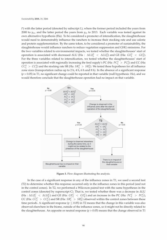
Sustainability 2018, 10, 3266
F) with the latter period (denoted by subscript L), where the former period included the years from2000 to yos, and the latter period the years from yos to 2013. Each variable was tested against itsown alternative hypothesis (Ha). To be considered a promoter of intensification, the slaughterhousewould need to demonstrably influence the ranchers to increase their stocking rate and use calorieand protein supplementation. By the same token, to be considered a promoter of sustainability, theslaughterhouse would influence ranchers to reduce vegetation suppression and GHG emissions. Forthe two variables related to environmental impacts, we tested whether the slaughterhouses’ start ofoperation is associated with decreased ΔLU (Ha : ΔLUS
L < ΔLUSF) and GE (Ha: GES
L < GESF).
For the three variables related to intensification, we tested whether the slaughterhouses’ start ofoperation is associated with regionally increasing the feed supply’s PC (Ha: PCS
L > PCSF) and CC (Ha:
CCSL > CCS
F) and the stocking rate SR (Ha: SRSL > SRS
F). We tested these hypotheses for all influencezone sizes (transportation radius up to 2 h, 4 h, 6 h and 8 h). In the absence of a significant response(p > 0.05) in T1, no significant change could be reported in that variable (null hypothesis: Ho), and wewould therefore conclude that the slaughterhouse operation had no impact on that variable.
Figure 3. Flow diagram illustrating the analysis.
In the case of a significant response in any of the influence zones in T1, we used a second test(T2) to determine whether this response occurred only in the influence zones in this period (and notin the control zones). In T2, we performed a Wilcoxon paired test with the same hypotheses in thecontrol zones (denoted by superscript C). That is, we tested whether there was a decrease in ΔLU(Ha : ΔLUC
L < ΔLUCF ) and GE (Ha: GEC
L < GECF ) and an increase in the PC (Ha: PCC
L > PCCF ),
CC (Ha: CCCL > CCC
F ) and SR (Ha: SRCL > SRC
F ) observed within the control zones between thesetime periods. A significant response (p ≤ 0.05) in T2 means that the change in this variable was alsoobserved elsewhere in the biome, outside of the influence zones, so it might not be directly related tothe slaughterhouse. An opposite or neutral response (p > 0.05) means that the change observed in T1
98

Sustainability 2018, 10, 3266
occurred only in the slaughterhouse influence zone, and, in these cases, we would conclude that theslaughterhouse had an impact on the variable.
3. Results
3.1. Influence and Control Zones
Figure 4 shows the 12 influence zones obtained. The average sizes of the influence zones fortravel times up to 2 h, 4 h, 6 h and 8 h are 0.43 Mha, 1.7 Mha, 4.1 Mha and 7.3 Mha, respectively.As the delimited extents were based on the travel time of a truck, the sizes of the influence zones varyaccording to the road network present near each slaughterhouse.
Due to the proximity between the slaughterhouse units, there are overlaps in some influencezones. However, just two zones (4267 and 791) have more than 50% of the 8 h zone shared by both(Figure 4). As the overlap starts at the 4 h travel time, we decided to keep the units separated instead ofjoining them so that the analysis has the same number of units per size of influence zone. In addition,the zones under the influence of slaughterhouses identified by SIF codes 1940, 3348 and 4333 extendover both biomes. However, just the 1940 SIF code unit was considered in both biome analyses, as alarge percentage of its 8 h area is in the Cerrado biome (60% of the 8 h zone). Thus, five slaughterhouseswere evaluated for the Cerrado, and eight for the Amazon.
Figure 4. Locations of selected large slaughterhouses and their influence zones. Solid and dashed linesrepresent the paved and unpaved roads, respectively.
When choosing the control zones, first we excluded 340 Mha in both biomes, 70% in conservationunits and indigenous lands and 30% in areas under the influence of selected slaughterhouses and
99

Sustainability 2018, 10, 3266
slaughterhouses with yos before 2000. We chose eight control areas in the Amazon and five controlareas in the Cerrado (Figure 5). The selected zones have an average size of 7.3 Mha, the same as theaverage size of the 8 h influence zones.
Figure 5. Locations of the control zones. The black squares indicate the zone limits. Green areasindicate areas with the potential to be control zones. White areas indicate influence zones of selectedslaughterhouses and slaughterhouses with yos before 2000.
3.2. Statistical Analysis
In the following sections, we show the results for each influence zone and control zone, separatedby variable. Negative differences indicate a decrease in the variable analyzed with time.
3.2.1. Environmental Impact Variable: Land Use Change Rate (ΔLU)
Table 3 shows ΔLUF and ΔLUL results for the influence zones and the control zones. The first test(T1), a Wilcoxon paired test, determines whether there is a decrease in ΔLU inside the influence zonesafter the slaughterhouse start of operation. In Amazonia, there is a decrease in ΔLU in all influencezone sizes (travel times up to 2 h, 4 h, 6 h and 8 h), with similar values of probability (p = 0.004,Table 4). These results across the various sizes of the influence zones indicate that the distance fromthe slaughterhouse unit does not influence ΔLU. Results from T2 show that the decrease of ΔLU alsooccurs inside the control zones (p = 0.008, Table 4). The similar responses in both the slaughterhouseinfluence zones and the control zones during the same period indicate that the decrease of ΔLU mightbe not related to the slaughterhouse presence.
100

Sustainability 2018, 10, 3266
Ta
ble
3.
Form
eran
dla
tter
peri
odva
lues
for
land
use
chan
gera
te(Δ
LU,i
nha
/yea
r)fo
rea
chin
fluen
cezo
nean
dco
ntro
lzon
e.
2h
4h
6h
8h
Co
ntr
ol
SIF
Co
de
ΔLU
S F(h
a/
year )
ΔLU
S L(h
a/
year )
ΔLU
S F(h
a/
year )
ΔLU
S L(h
a/
year )
ΔLU
S F(h
a/
year )
ΔLU
S L(h
a/
year )
ΔLU
S F(h
a/
year )
ΔLU
S L(h
a/
year )
Co
ntr
ol
Co
de
ΔLU
C F(h
a/
year )
ΔLU
C L(h
a/
year )
791
6557
.552
2387
.213
28,4
46.3
3288
36.6
5061
,395
.094
19,9
53.5
0092
,905
.984
30,8
94.8
441
80,3
72.4
8447
,051
.168
3348
9407
.771
1465
.027
34,1
95.2
7776
76.2
2682
,200
.266
18,9
56.4
9013
7,13
6.98
442
,684
.102
281
,378
.305
53,3
18.9
8830
4794
6.86
111
35.2
8852
35.6
9750
93.8
2314
,266
.354
11,8
52.6
0125
,618
.500
21,0
87.4
883
15,8
19.8
6416
,464
.074
137
250.
060
735.
411
1786
.634
3959
.375
7293
.791
11,7
91.5
6817
,400
.232
25,3
62.8
594
59,5
20.3
2446
,821
.258
1723
1816
.823
1779
.501
9388
.703
8416
.078
22,9
71.7
7919
,033
.506
36,7
94.2
7331
,167
.559
559
,506
.941
50,9
30.0
3118
8618
68.6
2313
62.5
0296
10.9
3759
00.3
0920
,900
.621
12,6
23.7
5635
,851
.840
22,3
29.5
536
117,
978.
461
46,4
30.7
8519
4015
76.9
7814
39.5
1710
,806
.022
8332
.689
26,2
63.9
9418
,966
.988
55,3
17.7
5835
,559
.426
710
5,35
5.86
738
,125
.027
2583
2439
.150
563.
163
9376
.688
2705
.178
23,0
52.0
8077
71.4
1342
,548
.234
14,2
80.6
468
30,9
46.5
2119
,714
.889
2937
781.
155
469.
791
5982
.479
2420
.442
22,7
98.0
9485
78.5
4756
,155
.816
18,5
31.9
349
35,7
76.4
2638
,022
.645
4149
4107
.312
2648
.438
18,2
82.7
6211
,317
.136
39,1
51.1
1724
,151
.670
79,5
50.4
5341
,369
.051
1039
,928
.773
36,6
83.5
3942
6735
96.0
0317
93.6
4524
,930
.428
8992
.448
64,3
70.4
2620
,787
.986
122,
377.
789
38,6
33.9
2211
34,8
75.1
8835
,362
.727
4333
7961
.677
3783
.414
22,3
55.8
1810
,142
.759
47,4
14.7
0718
,169
.438
76,8
47.1
4127
,719
.873
1229
,021
.994
36,1
96.1
9913
22,4
20.3
9632
,550
.551
101

Sustainability 2018, 10, 3266
Table 4. Results of Wilcoxon paired tests for T1 and T2 for land use change rate (ΔLU). T1 tests whetherthe introduction of large slaughterhouses was associated with the reduction of ΔLU in the influencezones (Ha: ΔLUS
L < ΔLUSF ). T2 tests whether reduction of ΔLU also occurred in the control zones (Ha:
ΔLUCL < ΔLUC
F ).
Latter Values–Former Values (ΔLU)
T1(
Ha : ΔLUSL < ΔLUS
F
)T2
(Ha : ΔLUC
L < ΔLUCF
)
SIFCode
2 h (ha/year) 4 h (ha/year) 6 h (ha/year) 8 h (ha/year)Control
CodeControl
(ha/year)
Amazonia
791 −4170.339 −19,609.682 −41,441.594 −62,011.140 1 −33,321.3163348 −7942.744 −26,519.051 −63,243.776 −94,452.882 2 −28,059.3171940 −137.461 −2473.333 −7297.006 −19,758.332 3 644.2102583 −1875.987 −6671.510 −15,280.667 −28,267.588 4 −12,699.0662937 −311.364 −3562.037 −14,219.547 −37,623.882 5 −8576.9104149 −1458.874 −6965.626 −14,999.447 −38,181.402 6 −71,547.6764267 −1802.358 −15,937.980 −43,582.440 −83,743.867 7 −67,230.8404333 −4178.263 −12,213.059 −29,245.269 −49,127.268 8 −11,231.632
Median −1839.173 −9589.343 −22,262.968 −43,654.335 −20,379.192
p 0.004 * 0.004 * 0.004 * 0.004 * 0.008 *
Cerrado
3047 188.427 −141.874 −2413.753 −4531.012 9 2246.219137 485.351 2172.741 4497.777 7962.627 10 −3245.2341723 −37.322 −972.625 −3938.273 −5626.714 11 487.5391886 −506.121 −3710.628 −8276.865 −13,522.287 12 7174.2051940 −137.461 −2473.333 −7297.006 −19,758.332 13 10,130.155
Median −37.322 −972.625 −3938.273 −5626.714 2246.219
p 0.500 NS 0.156 NS 0.156 NS 0.156 NS 0.906 NS
* Indicates significant at 5% level. NS Indicates not significant at 5% level. SIF code 1940 is used in the analyses ofboth biomes.
In the Cerrado, T1 shows no decrease in ΔLU (Table 4). This indicates that the slaughterhouseshad no impact on ΔLU inside the slaughterhouse influence zones. Although a drop in ΔLU is observedin most of the influence zones, due to the small size of the sample, the response is not significant. Bycomparison, the T2 test shows interesting results: most of the control zones show increases in ΔLU.Of the five control zones, four show increases in ΔLU in the latter part of the study period (p = 0.906,Table 4).
3.2.2. Environmental Impact Variable: Total Greenhouse Gas Emissions (GE)
Table 5 shows GEF and GEL results for the influence zones and control zones. In the Amazon, T1results show that there is a significant reduction of GE after the slaughterhouses’ start of operation. Asoccurred with tests for ΔLU, all zones show the same level of significance, which demonstrates theabsence of a distance influence (p = 0.004, Table 6). The similar responses between ΔLU and GE werealready expected because of the large contribution of land use emissions to the total emissions. Afterfinding a significant response in the 8 h influence zone for T1, WE used T2 to compare this result withthe response in control areas outside the slaughterhouse influence zones. As occurred with ΔLU, T2results confirm that the decrease of GE also occurred in the control zones (p = 0.008, Table 6). The T1and T2 responses demonstrate that the change is observed both inside and outside of the influencezones during the same period, so the decrease of GE might be unrelated to the slaughterhouse presence.
102

Sustainability 2018, 10, 3266
Ta
ble
5.
Form
eran
dla
tter
peri
odva
lues
for
gree
nhou
sega
sem
issi
ons
(GE,
inTg
-CO
2e/y
ear)
for
each
influ
ence
zone
and
cont
rolz
one.
2h
4h
6h
8h
Co
ntr
ol
SIF
Co
de
GES F
(Tg
-CO
2e/y
ea
r)G
ES L(T
g-C
O2e/y
ea
r)G
ES F(T
g-C
O2e/y
ea
r)G
ES L(T
g-C
O2e/y
ea
r)G
ES F(T
g-C
O2e/y
ea
r)G
ES L(T
g-C
O2e/y
ea
r)G
ES F(T
g-C
O2e/y
ea
r)G
ES L(T
g-C
O2e/y
ea
r)C
on
tro
lC
od
eG
EC F(T
g-C
O2e/y
ea
r)G
EC L(T
g-C
O2e/y
ea
r)
791
4.8
2.5
198.
238
1757
241
5936
3348
5.6
0.93
204.
444
1170
242
5839
3047
0.35
0.35
1.9
1.7
5.1
4.4
109.
33
6.1
7.0
137
0.14
0.19
0.86
1.1
3.2
3.9
7.3
8.8
442
3417
230.
500.
552.
32.
45.
95.
610
9.6
537
3218
860.
960.
843.
32.
76.
04.
79.
67.
66
6428
1940
1.0
0.87
6.1
4.2
149.
428
167
6927
2583
1.9
0.58
7.6
2.9
187.
833
148
1811
2937
0.73
0.53
4.1
2.3
146.
930
139
1516
4149
2.3
1.4
9.5
5.6
2213
4624
107.
76.
842
673.
02.
018
9.1
4319
7831
119.
39.
443
334.
22.
112
5.7
2511
4118
127.
38.
313
3.9
5.4
103

Sustainability 2018, 10, 3266
Table 6. Results of Wilcoxon paired tests for T1 and T2 for greenhouse gas emissions (GE). T1 testswhether the introduction of large slaughterhouses was associated with the reduction of GE in theinfluence zones (Ha: GES
L < GESF) T2 tests whether reduction of GE also occurred in the control zones
(Ha: GECL < GEC
F ).
Latter Values–Former Values (GE)
T1(
Ha : GESL < GES
F
)T2 (Ha: GEC
L < GECF )
SIF Code2 h
(Tg-CO2e/year)4 h
(Tg-CO2e/year)6 h
(Tg-CO2e/year)8 h
(Tg-CO2e/year)Control
CodeControl
(Tg-CO2e/year)
Amazonia
791 −2.3 −11 −22 −33 1 −233348 −4.7 −15 −33 −46 2 −191940 −0.13 −1.9 −4.8 −12 3 0.942583 −1.3 −4.6 −11 −19 4 −7.82937 −0.20 −1.8 −7.1 −17 5 −4.44149 −0.90 −3.8 −8.4 −22 6 −364267 −0.95 −8.8 −24 −47 7 −424333 −2.1 −5.9 −14 −23 8 −7.6
Median −1.1 −5.3 −12 −23 −13.6
p 0.004 * 0.004 * 0.004 * 0.004 * 0.008 *
Cerrado
3047 0.0010 −0.16 −0.69 −1.0 9 0.86137 0.048 0.28 0.71 1.5 10 −0.92
1723 0.046 0.075 −0.27 −0.70 11 0.141886 −0.12 −0.65 −1.2 −2.0 12 1.01940 −0.13 −1.9 −4.8 −12 13 1.6
Median 0.0010 −0.16 −0.69 −1.0 0.86
p 0.406 NS 0.219 NS 0.156 NS 0.156 NS 0.969 NS
* Indicates significant at 5% level. NS Indicates not significant at 5% level. SIF code 1940 is used in the analyses ofboth biomes.
In the Cerrado, T1 results show a nonsignificant response for the reduction of GE inside theslaughterhouse influence zones. As occurred in Amazonia, the GE results are very similar to the ΔLUresults. In addition, for transportation distances up to 4 h, emissions due to enteric fermentationappear to have a greater influence on the total emitted. In comparison to what was observed for ΔLU,where two units show increases inside the influence zones up to 2 h and one up to 4 h, for GE, threeunits (SIF codes 3047, 137 and 1723) show increases in GE inside the zones up to 2 h, and two (SIFcodes 137 and 1723) in the zones up to 4 h. According to the analysis framework, the T2 test is notnecessary in the case of negative responses up to 8 h. As was the case with ΔLU analyses, T2 resultslooking at GE show that the increases also occur inside the control zones (p = 0.969, Table 6).
3.2.3. Intensification Variable: Protein from Crops (PC)
Table 7 shows PCF and PCL results for the influence zones and control zones. In Amazonia, T1results show that there was a change in PC inside the influence zones (p ≤ 0.05, Table 8). In addition,the decrease of p with the increase of influence zone sizes (up to 2 h, 4 h, 6 h, and 8 h) indicates thatdistance from the slaughterhouse unit had a likely influence. As T1 results show significant changesin PC in the influence zones, we use T2 to determine whether the changes occurred only inside theinfluence zones. According to T2 results, the increase of PC also occurred in the control zones (p ≤ 0.05,Table 8), which implies the absence of slaughterhouse impact on this variable.
104

Sustainability 2018, 10, 3266
Ta
ble
7.
Form
eran
dla
tter
peri
odva
lues
for
prot
ein
from
crop
s(P
C,i
nG
gpr
otei
n)fo
rea
chin
fluen
cezo
nean
dco
ntro
lzon
e.
2h
4h
6h
8h
Co
ntr
ol
SIF
Co
de
PC
S F(G
g)
PC
S L(G
g)
PC
S F(G
g)
PC
S L(G
g)
PC
S F(G
g)
PC
S L(G
g)
PC
S F(G
g)
PC
S L(G
g)
Co
ntr
ol
Co
de
PC
C F(G
g)
PC
C L(G
g)
791
8.7
1521
3836
6763
1.2×
102
117
3733
4842
1.1×
102
2.6×
102
5.1×
102
6.2×
102
1.1×
103
1.0×
103
1.8×
103
26.
518
3047
891.
2×
102
3.7×
102
4.9×
102
9.3×
102
1.2×
103
1.5×
103
2.0×
103
30.
201.
013
732
491.
5×
102
2.5×
102
4.2×
102
7.2×
102
7.5×
102
1.3×
103
414
2217
233.
310
1336
2877
551.
4×
102
52.
03.
118
861.
0×
102
1.5×
102
3.5×
102
4.8×
102
7.1×
102
9.5×
102
1.1×
103
1.4×
103
65.
6×
102
1.3×
103
1940
1.2
2.5
6.4
1434
7087
1.7×
102
778
1.3×
102
2583
0.20
0.19
1.4
1.4
4.0
4.2
8.5
108
4.4
4.4
2937
1.2
2.7
1025
3595
782.
2×
102
928
8041
490.
170.
210.
360.
570.
681.
31.
63.
010
2.8×
102
5.6×
102
4267
1.1
1.1
7.3
1021
3532
6111
3.2×
102
5.3×
102
4333
1637
631.
3×
102
1.6×
102
2.8×
102
3.4×
102
5.4×
102
123.
2×
102
5.1×
102
131.
0×
102
2.7×
102
105

Sustainability 2018, 10, 3266
Table 8. Results of Wilcoxon paired tests for T1 and T2 for proteins from crops (PC). T1 tests whetherthe introduction of large slaughterhouses was associated with the increase of PC in the influencezones (Ha: PCS
L > PCSF). T2 tests whether the increase of PC also occurred in the control zones (Ha:
PCCL > PCC
F ).
Latter Values–Former Values (PC)
T1 (Ha: PCSL > PCS
F) T2 (Ha: PCCL > PCC
F )
SIF Code 2 h (Gg) 4 h (Gg) 6 h (Gg) 8 h (Gg) Control Code Control (Gg)
Amazonia
791 6.3 17 32 59 1 203348 66 2.6 × 10² 5.2 × 10² 8.3 × 10² 2 111940 1.3 7.6 36 83 3 0.782583 −0.011 −0.050 0.19 1.8 4 7.42937 1.5 16 60 1.4 × 10² 5 1.14149 0.049 0.21 0.57 1.4 6 7.1 × 10²
4267 −0.032 2.5 14 30 7 514333 21 70 1.3 × 10² 1.9 × 10² 8 −0.069
Median 1.4 12 34 71 9.3
p 0.020 * 0.008 * 0.004 * 0.004 * 0.008 *
Cerrado
3047 32 1.2 × 10² 2.8 × 10² 4.9 × 10² 9 51137 17 1.0 × 10² 3.0 × 10² 5.1 × 10² 10 2.9 × 10²
1723 7.0 23 49 88 11 2.1 × 10²
1886 43 1.4 × 10² 2.4 × 10² 3.5 × 10² 12 1.9 × 10²
1940 1.3 7.6 36 83 13 1.7 × 10²
Median 17 1.0 × 10² 2.4 × 10² 3.5 × 10² 1.9 × 10²
p 0.031 * 0.031 * 0.031 * 0.031 * 0.031 *
* Indicates significant at 5% level. SIF code 1940 is used in the analyses of both biomes.
In the Cerrado, based on T1, all sizes of influence zone show an increase in PC after theslaughterhouse start of operation at the same level of significance (Table 8). The T2 results indicate asimilar increase of PC occurred inside the control zones (p ≤ 0.05, Table 8). These similar responsesindicate that the large slaughterhouses have no impact on the PC.
3.2.4. Intensification Variable: Calories from Crops (CC)
Table 9 shows CCF and CCL results for the study influence zones and control zones. In Amazonia,T1 shows that there is an increase in CC in all influence zone sizes (up to 2 h, 4 h, 6 h and 8 h). Asoccurred with PC, there is an influence of distance from the slaughterhouse, with p decreasing alongwith increase of zone size. T2 shows that the increase in CC between the two time periods also occursinside the control zones (p = 0.020, Table 10). The similar responses in T1 and T2 indicate that theincrease of CC might not be related to the slaughterhouse presence.
106

Sustainability 2018, 10, 3266
Ta
ble
9.
Form
eran
dla
tter
peri
odva
lues
for
calo
ries
from
crop
s(C
C,i
nPc
al)f
orea
chin
fluen
cezo
nean
dco
ntro
lzon
e.
2h
4h
6h
8h
Co
ntr
ol
SIF
Co
de
CC
S F(P
cal )
CC
S L(P
cal )
CC
S F(P
cal )
CC
S L(P
cal )
CC
S F(P
cal )
CC
S L(P
cal )
CC
S F(P
cal )
CC
S L(P
cal )
Co
ntr
ol
Co
de
CC
C F(P
cal )
CC
C L(P
cal )
791
0.13
0.24
0.33
0.58
0.53
1.0
0.84
1.6
10.
470.
7733
480.
391.
22.
45.
65.
812
1020
20.
170.
3230
471.
11.
84.
47.
411
1818
303
0.00
670.
015
137
0.45
0.74
2.1
3.6
5.3
9.7
1017
40.
290.
3317
230.
037
0.10
0.15
0.36
0.34
0.78
0.75
1.7
50.
057
0.07
018
861.
11.
73.
75.
77.
311
1117
65.
414
1940
0.01
60.
029
0.09
20.
170.
470.
821.
11.
97
0.77
1.3
2583
0.00
630.
0058
0.04
30.
039
0.11
0.11
0.22
0.22
80.
070
0.05
629
370.
017
0.03
10.
110.
280.
371.
00.
802.
49
0.80
1.7
4149
0.00
520.
0055
0.01
10.
015
0.02
10.
030
0.04
80.
067
103.
06.
142
670.
034
0.03
30.
180.
220.
380.
580.
520.
9311
3.3
5.6
4333
0.16
0.41
0.62
1.5
1.6
3.2
3.4
6.0
123.
85.
813
1.1
2.9
107

Sustainability 2018, 10, 3266
Table 10. Results of Wilcoxon paired tests for T1 and T2 for calories from crops (CC). T1 tests whetherthe introduction of large slaughterhouses was associated with the increase of CC in the influencezones (Ha: CCS
L > CCSF).T2 tests whether the increase of CC also occurred in the control zones (Ha:
CCCL > CCC
F ).
Latter Values–Former Values (CC)
T1 (Ha: CCSL > CCS
F) T2 (Ha: CCCL > CCC
F )
SIF Code 2 h (Pcal) 4 h (Pcal) 6 h (Pcal) 8 h (Pcal) Control Code Control (Pcal)
Amazonia
791 0.10 0.26 0.45 0.79 1 0.303348 0.78 3.2 6.6 11 2 0.141940 0.012 0.073 0.35 0.86 3 0.00852583 −0.00056 −0.0043 −0.0065 −0.0022 4 0.0372937 0.014 0.17 0.67 1.6 5 0.0134149 0.00027 0.0034 0.0090 0.019 6 8.84267 −0.0012 0.045 0.20 0.40 7 0.584333 0.26 0.86 1.6 2.7 8 −0.014
Median 0.013 0.12 0.40 0.82 0.090
p 0.039 * 0.012 * 0.008 * 0.008 * 0.020 *
Cerrado
3047 0.76 3.0 7.3 13 9 0.90137 0.28 1.5 4.3 7.9 10 3.1
1723 0.063 0.21 0.43 0.91 11 2.31886 0.58 1.9 3.8 5.9 12 2.11940 0.012 0.073 0.35 0.86 13 1.8
Median 0.28 1.5 3.8 5.9 2.1
p 0.031 * 0.031 * 0.031 * 0.031 * 0.031 *
* Indicates significant at 5% level. SIF code 1940 is used in the analyses of both biomes.
In the Cerrado, T1 shows that there is an increase in CC (Table 10). All influence zones show asignificant response in T1, which indicates a change occurred after slaughterhouse start of operation.As the response of the 8 h influence zone is significant, we use T2 results to determine whether theobserved result also occurred inside the control zones. The T2 results do indicate an increase of CC inthe control zones (p ≤ 0.05, Table 10), which means that the increase of CC might be unrelated to theslaughterhouse presence.
3.2.5. Intensification Variable: Stocking Rate (SR)
Table 11 shows SRF and SRL results for the study influence zones and control zones. In Amazonia,T1 results indicate that SR is not impacted by the slaughterhouse start of operation, with all sizes ofinfluence zone showing nonsignificant responses for the change (p > 0.05, Table 12). As T1 is negative,T2 is not necessary to prove the impact of the slaughterhouse. However, contrary to the results for theslaughterhouse influence zones, the control zones show a significant increase in the SR between timeperiods (p ≤ 0.05, Table 12).
108

Sustainability 2018, 10, 3266
Ta
ble
11
.Fo
rmer
and
latt
erpe
riod
valu
esfo
rst
ocki
ngra
te(S
R,i
nhe
ad/h
a)fo
rea
chin
fluen
cezo
nean
dco
ntro
lzon
e.
2h
4h
6h
8h
Co
ntr
ol
SIF
Co
de
SRS F
(head
/ha)
SRS L
(head
/ha)
SRS F
(head
/ha)
SRS L
(head
/ha)
SRS F
(head
/ha)
SRS L
(head
/ha)
SRS F
(head
/ha)
SRS L
(head
/ha)
Co
ntr
ol
Co
de
SRC F
(head
/ha)
SRC L
(head
/ha)
791
2.02
31.
915
1.99
01.
855
1.94
61.
856
1.93
61.
873
10.
981
1.07
333
480.
717
0.75
30.
867
0.91
51.
066
1.11
71.
194
1.24
02
1.20
41.
554
3047
0.87
51.
002
0.95
31.
055
0.96
81.
059
1.03
31.
124
30.
249
0.28
613
71.
011
1.25
70.
866
1.14
30.
821
1.11
90.
886
1.18
44
1.45
21.
504
1723
0.81
11.
060
0.85
81.
181
0.84
51.
144
0.83
41.
115
51.
342
1.68
418
861.
543
2.03
31.
130
1.43
30.
980
1.18
60.
921
1.07
36
1.45
81.
588
1940
0.98
41.
043
0.99
31.
081
1.02
51.
146
1.02
41.
150
71.
589
2.01
825
832.
532
2.67
21.
817
1.77
41.
628
1.52
21.
509
1.42
38
0.58
41.
453
2937
2.08
51.
850
1.91
31.
744
1.78
21.
719
1.70
81.
728
90.
968
1.26
741
491.
347
1.66
81.
407
1.60
41.
421
1.69
11.
577
1.90
210
0.65
60.
905
4267
1.82
61.
925
1.83
51.
971
1.86
62.
014
1.85
52.
036
110.
653
0.97
443
331.
237
1.07
51.
756
1.72
11.
869
1.81
51.
794
1.82
112
0.61
20.
936
130.
512
0.53
0
109

Sustainability 2018, 10, 3266
Table 12. Results of Wilcoxon paired test for T1 and T2 for stocking rate (SR). T1 tests whether theintroduction of large slaughterhouses was associated with the increase of SR in the influence zones (Ha:SRS
L > SRSF). T2 tests whether the increase of SR also occurred in the control zones (Ha: SRC
L > SRCF ).
Latter Values–Former Values (SR)
T1 (Ha: SRSL > SRS
F) T2 (Ha: SRCL > SRC
F )
SIF Code2 h
(Head/ha)4 h
(Head/ha)6 h
(Head/ha)8 h
(Head/ha)Control
CodeControl
(Head/ha)
Amazonia
791 −0.108 −0.135 −0.090 −0.063 1 0.0923348 0.036 0.048 0.051 0.046 2 0.3501940 0.059 0.088 0.121 0.126 3 0.0372583 0.140 −0.043 −0.106 −0.086 4 0.0522937 −0.235 −0.169 −0.063 0.020 5 0.3424149 0.321 0.197 0.270 0.325 6 0.1304267 0.099 0.136 0.148 0.181 7 0.4294333 −0.162 −0.035 −0.054 0.027 8 0.869
Median 0.048 0.007 −0.002 0.037 0.236
p 0.473 NS 0.371 NS 0.320 NS 0.125 NS 0.004 *
Cerrado
3047 0.127 0.102 0.091 0.091 9 0.299137 0.246 0.277 0.298 0.298 10 0.2491723 0.249 0.323 0.299 0.281 11 0.3211886 0.490 0.303 0.206 0.152 12 0.3241940 0.059 0.088 0.121 0.126 13 0.018
Median 0.246 0.277 0.206 0.152 0.299
p 0.031 * 0.031 * 0.031 * 0.031 * 0.031 *
* Indicates significant at 5% level. NS Indicates not significant at 5% level. SIF code 1940 is used in the analyses ofboth biomes.
In the Cerrado, all sizes of influence zone show an increase in SR after the start of operation ofthe slaughterhouses studied (p = 0.031, Table 12). According to T2, the control zones have the sameresults as the influence zones (p = 0.031, Table 12). These similar responses indicate that the largeslaughterhouses are not directly responsible for SR increases in their influence zones in the Cerrado.
4. Discussion
Regarding the hypothesis that large slaughterhouses promote sustainable agriculturaldevelopment and cattle ranching intensification, we expected to find significant reductions invariables that measured environmental impact (ΔLU and GE) and increases in variables that measuredintensification (PC, CC, and SR) after the start of slaughterhouse operations. In Amazonia, the resultsshow that there is a significant decrease in ΔLU and GE inside the slaughterhouse influence zones.However, since the same change happened in the control zones, this decrease might not be causeddirectly by the slaughterhouse presence, and might instead be part of the downward trend ofdeforestation over the period between 2004 and 2013 [31,32]. For agricultural intensification variablesin Amazonia, PC and CC show a significant increase in both the influence and control zones, whileSR does not show change in the areas under slaughterhouse influence. In the Cerrado, results for allvariables are similar in the control and influence zones. Nonsignificant decreases in ΔLU and GE andsignificant increases of PC, CC, and SR are observed in the control zones as well as the influence zones.
The decrease in ΔLU observed both inside and outside the slaughterhouse influence zones inAmazonia demonstrates not slaughterhouse influence, but the power of conservation programsand other policies for forest protection [31,33–35]. In addition to the protection granted by theBrazilian Forest Code and monitoring programs such as the Program for Satellite Monitoring ofthe Brazilian Amazon Forest (PRODES—Projeto de Monitoramento da Floresta Amazônica Brasileirapor Satélite) and the System for Detection of Deforestation in Real Time (DETER—System for Detectionof Deforestation in Real Time), the private sector signed ambitious agreements—cattle agreements
110

Sustainability 2018, 10, 3266
in 2009 and a Soy Moratorium in 2006 [36]—to further protect the native vegetation. The effectivecontribution of each measure is difficult to disentangle, but the combined result of these actions was agreat success. According to INPE [32] the rate of forest loss in the Brazilian Amazon dropped frommore than 2.7 Mha/year in 2004 to an average of 0.6 Mha/year in 2013, reaching the lowest ratessince 1988.
Unfortunately, the same did not occur in the Cerrado. The decrease of ΔLU did not happen insideall influence zones. In the control zones, the ΔLU results indicate that there is increased suppressionof Cerrado vegetation in areas away from large slaughterhouse influence. This may be linked withthe absence of an effective vegetation suppression monitoring system in the biome, and the morepermissive New Forest Code, which has allowed more legal suppression since 2012 [35]. Somestudies [36,37] have also warned about a possible leakage of agriculture from Amazonia to the Cerradodue to the stricter conservation policies in Amazonia. According to the most recent official dataavailable, 0.725 Mha was suppressed in the Cerrado between 2010 and 2011, which was 12% greaterthan observed in the previous period (0.647 Mha, between 2009 and 2010 [38]. In addition, a recentreport released by Mighty Earth and Rainforest Foundation Norway (RFN) claimed that multinationalcompanies are linked to massive and systematic suppression of native vegetation in areas of Cerradoin MATOPIBA (an acronym created from the first two letters of the states of Maranhão, Tocantins,Piauí and Bahia). The report found that areas operated by the investigated companies had 0.697 Mhaof vegetation suppressed from 2011 to 2015 [39].
GE results reflect ΔLU results, as land use emissions dominate GE in both biomes. In Amazonia,even with the increase of cattle between 2000 and 2013 (from 29 to 56 million head), the emissions fromenteric fermentation are not enough to exceed the emissions from land use; this result was expecteddue to the high Amazonian biomass. In the Cerrado, the emissions from enteric fermentation dominateGE in the influence zones up to 4 h. For GE, by contrast with the results observed for ΔLU, threeslaughterhouse units showed an increase in the areas of influence up to a 2 h driving radius, and two,in a radius up to 4 h. This response suggests that, in the zones near the slaughterhouses, the nativevegetation has already been suppressed for the most part, making the emissions contributions fromenteric fermentation more prominent than those from land use change.
The PC and CC results show that there has been an increase in the production of protein andcalories in both biomes. In Amazonia, the p calculated for the various influence zone sizes show thatthe farther the distance from the slaughterhouse, the greater the increase in both variables. The mostlikely reason for this is that areas closer to these slaughterhouses are dominated by pasture, whichis unlikely to be converted to new cropping areas. According to Dias et al. [11], the Amazon andCerrado experienced expansion of crop area and increase in production in recent decades, especiallyfor soybeans. Considering both biomes, soybean production grew from 7.4 million tons in 1990 toapproximately 45.2 million tons in 2010 [11]. As one could expect, our results indicate that the increasesof PC and CC are not related to the slaughterhouses’ presence. However, the large increases in cropproduction around slaughterhouses may contribute to future increases in animal feed availability inthe region.
The SR results for Amazonia indicate that these pastures have a stable stocking rate probablyrelated to stagnant cattle ranching technology. To complement the discussion about SR, we performedtwo additional tests. First, we performed a Mann−Whitney test to compare the SR of the control andinfluence zones before the year of start of operation. In this test, we aimed to verify whether the largeslaughterhouses we studied were installed in areas with high values of SR. According to the result(Table 13), before the slaughterhouse start of operation in the Amazon, the SR in the influence zoneswas greater than the SR observed in the control zones (p = 0.031, Table 13). This is an indication thatbig companies prefer to install slaughterhouse units in areas with high production, to ensure supply totheir large processing capacity.
111

Sustainability 2018, 10, 3266
Table 13. Results of Mann-Whitney test comparing SRSF and SRC
F in Amazonia.
Former Period (Ha: SRSF �= SRC
F )
SIF Code SRSF (Head/ha) Control Code SRC
F (Head/ha)
791 1.936 1 0.9813348 1.194 2 1.2041940 1.024 3 0.2492583 1.509 4 1.4512937 1.708 5 1.3424149 1.577 6 1.4584267 1.855 7 1.5894333 1.794 8 0.584
Median 1.643 1.273
p 0.031 *
* Indicates significant at 5% level.
In the second test (Table 14), to verify the stagnation of the SR inside the slaughterhouses influencezones, we performed a Mann–Whitney test to compare the SR of the control and influence zones afterthe start of slaughterhouse operations. The result shows that in the latter period, the SR values of thecontrol zones are similar to the values in the influence zones (p = 0.328, Table 14). In other words, andconsidering also the results of Table 12, stocking rate is intensifying at much faster rates away from thelarge slaughterhouses than closer to them.
Table 14. Results of Mann-Whitney test comparing the SRSL and SRC
L in Amazonia.
Latter Period (Ha: SRSL �= SRC
L )
SIF Code SRSL (Head/ha) Control Code SRC
L (Head/ha)
791 1.873 1 1.0733348 1.240 2 1.5541940 1.150 3 0.2862583 1.423 4 1.5042937 1.728 5 1.6844149 1.902 6 1.5884267 2.036 7 2.0184333 1.821 8 1.453
Median 1.775 1.529
p 0.328 NS
NS Indicates not significant at 5% level.
Our results also demonstrate that the relationship between SR and ΔLU is not easily defined.After the slaughterhouse start of operation in the Amazon, although ΔLU dropped everywhere, theprocess of intensification did not start in the influence zones. Through a historical comparison betweenthe US and Brazil, Merry and Soares [18] suggested that Brazilian cattle ranching will intensify as aresult of economic conditions and conservation investments (reductions in capital and land subsidies)rather than intensifying in order to produce conservation outputs. In addition, characteristics thatfacilitate extensive ranching practices need to be discouraged or removed. The relatively easy processof land acquisition—land grabbing and low land prices—accompanied by weak protection laws thatfacilitates forest clearing for new pasture areas are the main obstacles of intensive ranching profitability,and may continue to be so in the next years [10,40,41].
Finally, the main limitation of this work is related to three assumptions. First, as we assume thezone of slaughterhouse influence extends up to 8 h travel time from a slaughterhouse, we may haveexcluded pasture areas dedicated to the cow–calf segment of the market. This segment is the main
112

Sustainability 2018, 10, 3266
challenge on the pathway to achieving sustainable cattle ranching in Brazil, because it is not monitoredor tracked under the current cattle agreements [13]. In addition, nearly all cow–calf productioncontinues to be dependent on extensive grazing systems in the country [9].
Second, we may underestimate the area influenced by slaughterhouses, and therefore theappropriate sizes of the influence and control zones. We do not consider variables such as cattleavailability, market access and transportation cost in the zone size estimates. Today, about 49% ofactive slaughterhouses in Amazonia belong to companies that signed the TAC, corresponding to 70%of slaughter capacity in the biome [19]. Therefore, the similarities observed between the control andinfluence zones may indicate that small slaughterhouses, which are not considered in this analysis andmay be found inside some areas designated as control zones, may affect their supply areas in the sameway that large units do.
The third limitation is related to the assumption that only 12 selected slaughterhouses haveinfluence in their respective supply area. As observed in Figure 2, many large slaughterhouses arenear the selected ones and they may influence the variables analyzed along with the selected units.We assumed here that the effect of these older slaughterhouses has not changed in time, and the maineffect measured is due to the slaughterhouses that started operations in the period of analyses. Onlytwo slaughterhouses do not have other large units near them: SIF 4333 in Amazonia and SIF 3047 inthe Cerrado (Figure 2). Although it is not possible to test statistically one slaughterhouse, SIF 4333 hasthe same direction of change of the set of Amazonia plants for ΔLU, GE, PC and CC at all influencezones (Table 4, Table 6, Table 8, and Table 10) and for SR at the 6 h and 8 h influence zone (Table 12).Similar results are found for SIF 3047 when compared to the Cerrado set, except for ΔLU at the 2 hinfluence zone. This is an indication of the effectiveness of this assumption.
5. Conclusions
This study investigated the influence of large slaughterhouses on five variables, two related toenvironment impact (land use change rate and GHG emissions), and three related to cattle-ranchingintensification (protein from crops, calories from crops and stocking rate). The results indicate that thechanges observed inside the zones influenced by slaughterhouses cannot be attributed to the start ofslaughterhouse unit operation in either Amazonia or the Cerrado.
In the Amazon, the environmental impact variables we studied show the same pattern ofresponses inside and outside the slaughterhouse influence zones—both moving towards reducedenvironmental impact. The hypothesis that slaughterhouses are leverage points to reduce deforestationand suppression of native Cerrado vegetation is not confirmed, leading us to believe that conservationmeasures such as a strong monitoring system and more restrictive environmental policies are themain promoters of conservation in Amazonia. In addition, the slaughterhouses seem to have noeffect on cattle-ranching intensification. The high stocking rates observed in the period before theslaughterhouses’ start of operation indicate that large meatpackers prefer to set up their plants in areasalready well established and developed in the biome.
In the Cerrado, the responses of the environmental impact variables both inside and outside theslaughterhouse influence zones indicate that there is considerable conservation work to be done inthe biome. The success of sustainable agriculture in the Cerrado still relies on the implementationof conservation measures. In addition, the increase of PC, CC, and SR both inside and outside theinfluence zones demonstrates that, in the Cerrado, cattle-ranching intensification is a reality, and it isoccurring independently of the presence of large slaughterhouses.
In conclusion, there is no evidence that large slaughterhouses have promoted either cattle-ranchingintensification or improvements in the sustainability of cattle-ranching activity in the Amazon andCerrado. The results of our study and the recent failures of some of the cattle agreements showthat leaning on slaughterhouses should not be considered a reliable strategy to achieve sustainablebeef production. According to Lambin et al. [42], zero-deforestation agreements signed by privatesectors may not be sufficient to reduce environmental impacts in commodities supply chain; public
113

Sustainability 2018, 10, 3266
and private policies need to complement and reinforce each other to disconnect the link betweencattle production and deforestation. In addition, to achieve intensification, it is necessary to improvethe ranchers’ access to technologies and capital [43,44], as there are still too many cattle farmers inAmazonia and the Cerrado who are engaging in extensive ranching practices associated with lowincome and high environmental damage.
Author Contributions: A.B.S. and M.H.C. contributed equally to the design of the research, the analysis of theresults and the writing of the manuscript.
Funding: This research was funded by CNPq—Conselho Nacional de Desenvolvimento Científico e Tecnológico(process 134430/2015-8).
Conflicts of Interest: The authors declare no conflict of interest.
Appendix Table with All Abbreviations Used in the Text
ABBREVIATIONS
AGB Aboveground biomass
BGB Belowground biomass
CARCadastro Ambiental Rural
(Rural Environmental Registry)
CNPJCadastro Nacional de Pessoa Jurídica
(National Register of Legal Entities)
DETERSistema de Detecção de Desmatamento em Tempo Real
(System for the Detection of Deforestation in Real Time)
DIPOADepartamento de Inspeção de Produtos de Origem Animal
(Department for Inspection of Animal Products)
GHG Greenhouse Gases
GWP Global Warming Potential
IBGEInstituto Brasileiro de Geografia e Estatística(Brazilian Institute of Geography and Statistics)
INPEInstituto Nacional de Pesquisas Espaciais
(National Institute for Space Research)
IPCC Intergovernmental Panel on Climate Change
LULUCF Land Use, Land Use Change and Forestry
MAPAMinistério da Agricultura, Pecuária e Abastecimento
(Brazilian Ministry of Agriculture, Livestock and Food Supply)
MATOPIBAAcronym created from the first two letters of the states of Maranhão,
Tocantins, Piauí, and Bahia
NGOs Non-Governmental Organizations
PNLTPlano Nacional de Logística e Transporte(National Logistics and Transportation Plan)
PNMCPolítica Nacional sobre Mudanças no Clima
(Brazil’s National Policy on Climate Change)
PRODESProjeto de Monitoramento da Floresta Amazônica Brasileira por Satélite
(Program for Satellite Monitoring of the Brazilian Amazon Forest)
114

Sustainability 2018, 10, 3266
Appendix Biomass Map and Emissions from Enteric Fermentation
The biomass map of the historic vegetation for Amazonia and the Cerrado is presented inFigure A1. The historic carbon content of native vegetation was 68.7 Pg-C for Amazonia and 10.1 Pg-Cfor the Cerrado. Estimation of the historic vegetation is a complicated process, and results can varywidely. Our estimate is comprehended in the range calculate by Leite et al. [45] for Amazonia (from51.3 to 85.5 Pg-C); however, our estimate is about 53% less than the estimate for the Cerrado (from13.8 to 28.8 Pg-C). The historic carbon content of native vegetation estimated in this study is differentfrom the values reported in Leite et al. [45] because different methodologies and values of carbonstock were used to make the biomass maps. While Leite et al. [45] combined two maps of vegetationtypes (RadamBrasil and IBGE [25]) and used the values for carbon stock in vegetation from the SecondNational Communication of Brazil to the UNFCCC, we used the map from IBGE [25] and the datafrom the Third National Communication.
Figure A1. Biomass map for past vegetation of Amazonia and the Cerrado.
Another result is the CH4 emissions from enteric fermentation. Between 2000 and 2013, theemissions from beef cattle increased in both biomes. Total methane emission by the two biomes inthis period amounted to 2.9 Pg-CO2e, about 54% of the total emitted in the country (5.3 Pg-CO2e [2]).Emissions in Amazonia increased about 80% (from 41.7 Tg-CO2e in 2000 to 77.5 Tg-CO2e in 2013).In the Cerrado, emissions increased about 0.09% (from 82.5 Tg-CO2e in 2000 to 90.5 Tg-CO2e in 2013).The increase was bigger in the Amazon than in the Cerrado because of the great increase in number ofcattle that occurred in this period.
Our estimates for methane emissions are very similar to other data. According toAzevedo et al. [2], for the states of the Amazon biome, the total amount of methane emitted by entericfermentation from beef cattle was 1.0 Pg-CO2e for the period, while our estimate was 0.9 Pg-CO2e.
115

Sustainability 2018, 10, 3266
For the states of the Cerrado, Azevedo et al. [2] reported total methane emissions of 2.0 Pg-CO2-eqfor the period, about 35% greater than our estimate of about 1.3 Pg-CO2-eq. These Cerrado estimatesdiffer because we consider the actual geographic limits of the biome, while the Azevedo et al. [2] valueincludes total emissions for all Cerrado states, irrespective of how much area within the states is partof the Cerrado biome.
References
1. Ministério da Ciência, Tecnologia e Inovação. Third National Communication of Brazil to the United NationsFramework Convention on Climate Change; Ministério da Ciência, Tecnologia e Inovação: Brasilia, Brazil, 2016;Volume III, ISBN 9788588063198.
2. De Azevedo, T.R.; Costa Junior, C.; Brandão Junior, A.; Cremer, M.D.S.; Piatto, M.; Tsai, D.S.; Barreto, P.;Martins, H.; Sales, M.; Galuchi, T.; et al. SEEG initiative estimates of Brazilian greenhouse gas emissionsfrom 1970 to 2015. Sci. Data 2018, 5, 1–43. [CrossRef] [PubMed]
3. Cohn, A.S.; Mosnier, A.; Havlík, P.; Valin, H.; Herrero, M.; Schmid, E.; O’Hare, M.; Obersteiner, M.Cattle ranching intensification in Brazil can reduce global greenhouse gas emissions by sparing land fromdeforestation. Proc. Natl. Acad. Sci. USA 2014, 111, 7236–7241. [CrossRef] [PubMed]
4. Strassburg, B.B.N.; Latawiec, A.E.; Barioni, L.G.; Nobre, C.A.; da Silva, V.P.; Valentim, J.F.; Vianna, M.;Assad, E.D. When enough should be enough: Improving the use of current agricultural lands could meetproduction demands and spare natural habitats in Brazil. Glob. Environ. Chang. 2014, 28, 84–97. [CrossRef]
5. Crosson, P.; Shalloo, L.; O’Brien, D.; Lanigan, G.J.; Foley, P.A.; Boland, T.M.; Kenny, D.A. A review of wholefarm systems models of greenhouse gas emissions from beef and dairy cattle production systems. Anim. FeedSci. Technol. 2011, 166–167, 29–45. [CrossRef]
6. De Oliveira Silva, R.; Barioni, L.G.; Hall, J.A.J.; Matsuura, M.F.; Zanett Albertini, T.; Fernandes, F.A.; Moran, D.Increasing beef production could lower greenhouse gas emissions in Brazil if decoupled from deforestation.Nat. Clim. Chang. 2016, 6, 493–497. [CrossRef]
7. Mazzetto, A.M.; Feigl, B.J.; Schils, R.L.M.; Cerri, C.E.P.; Cerri, C.C. Improved pasture and herd managementto reduce greenhouse gas emissions from a Brazilian beef production system. Livest. Sci. 2015, 175, 101–112.[CrossRef]
8. Palermo, G.C.; D’Avignon, A.L.D.A.; Freitas, M.A.V. Reduction of emissions from Brazilian cattle raisingand the generation of energy: Intensification and confinement potentials. Energy Policy 2014, 68, 28–38.[CrossRef]
9. Ferraz, J.B.S.; de Felício, P.E. Production systems—An example from Brazil. Meat Sci. 2010, 84, 238–243.[CrossRef] [PubMed]
10. Bowman, M.S.; Soares-Filho, B.S.; Merry, F.D.; Nepstad, D.C.; Rodrigues, H.; Almeida, O.T. Persistence ofcattle ranching in the Brazilian Amazon: A spatial analysis of the rationale for beef production. Land UsePolicy 2012, 29, 558–568. [CrossRef]
11. Dias, L.C.P.; Pimenta, F.M.; Santos, A.B.; Costa, M.H.; Ladle, R.J. Patterns of land use, extensification, andintensification of Brazilian agriculture. Glob. Chang. Biol. 2016, 22, 2887–2903. [CrossRef] [PubMed]
12. Barreto, P.; Pereira, R.; Arima, E. A Pecuária e o Desmatamento na Amazônia na era das Mudanças Climáticas;Instituto do Homem e Meio Ambiente da Amazônia: Belém, Brazil, 2008; ISBN 9788586212260.
13. Gibbs, H.K.; Munger, J.; L’Roe, J.; Barreto, P.; Pereira, R.; Christie, M.; Amaral, T.; Walker, N.F. Did ranchersand slaughterhouses respond to zero-deforestation agreements in the Brazilian Amazon? Conserv. Lett. 2016,9, 32–42. [CrossRef]
14. Greenpeace. Eating up the Amazon. Available online: http://www.greenpeace.org/usa/research/eating-up-the-amazon/ (accessed on 16 May 2016).
15. Greenpeace. Slaughtering the Amazon. Available online: http://www.greenpeace.org/international/en/publications/reports/slaughtering-the-amazon/ (accessed on 16 May 2016).
16. Walker, N.; Patel, S.; Kalif, K. From Amazon pasture to the high street: Deforestation and the Brazilian cattleproduct supply chain. Trop. Conserv. Sci. 2013, 6, 446–467. [CrossRef]
17. Garcia, E.; Filho, F.S.V.R.; Mallmann, G.M.; Fonseca, F. Costs, benefits and challenges of sustainable livestockintensification in a major deforestation frontier in the Brazilian Amazon. Sustainability 2017, 9, 158. [CrossRef]
116

Sustainability 2018, 10, 3266
18. Merry, F.; Soares-Filho, B. Will intensification of beef production deliver conservation outcomes in theBrazilian Amazon? Elem. Sci. Anth. 2017, 5, 1–12. [CrossRef]
19. Barreto, P.; Pereira, R.; Brandão, A., Jr.; Baima, S. Os Frigoríficos vão Ajudar a Zerar o Desmatamento da Amazônia?Imazon: Belém, Brazil, 2017; ISBN 9788586212949.
20. Alves-Pinto, H.N.; Newton, P.; Pinto, L.F.G. Certifying Sustainability: Opportunities and Challenges for theCattle Supply Chain in Brazil; Research Program on Climate Change; Agriculture and Food Security (CCAFS):Copenhagen, Denmark, 2010; pp. 1–8.
21. Zu Ermgassen, E.K.H.J.; de Alcântara, M.P.; Balmford, A.; Barioni, L.; Neto, F.B.; Bettarello, M.M.F.; deBrito, G.; Carrero, G.C.; Florence, E.D.A.S.; Garcia, E.; et al. Results from on-the-ground efforts to promotesustainable cattle ranching in the Brazilian Amazon. Sustainability 2018, 10, 1301. [CrossRef]
22. Barreto, P.; Silva, D. Will cattle ranching continue to drive deforestation in the Brazilian Amazon?In Environment and Natural Resources Management in Developing and Transition Economies; Centre of Studiesand Research on International Development from the University of Auvergne: Clermont Ferrand, France,2010; pp. 1–23.
23. Hansen, M.C.; Potapov, P.V.; Moore, R.; Hancher, M.; Turubanova, S.A.; Tyukavina, A.; Thau, D.;Stehman, S.V.; Goetz, S.J.; Loveland, T.R.; et al. High-Resolution Global Maps of 21st-Century ForestCover Change. Science 2013, 342, 850–853. [CrossRef] [PubMed]
24. Bustamante, M.; Santos, M.M.D.O.; Shimbo, J.Z.; Cantinho, R.Z.; Mello, T.D.R.B.D.; Oliveira, P.V.D.C.;Cunha, P.W.P.D.M.; Martins, F.D.S.R.V.; Aguiar, A.P.D.; Ometto, J. Emissões do Setor de uso da Terra, Mudançado uso da Terra e Florestas: Relatório de Referência; Ministério da Ciência, Tecnologia e Inovação: Brasíla, Brazil,2015; p. 343.
25. IBGE. Mapa de Vegetação. 2004. Available online: https://mapas.ibge.gov.br/tematicos/vegetacao(accessed on 13 February 2016).
26. Berndt, A.; Lemes, A.P.; Romero, L.A.; Sakamoto, L.S.; Lima, M.A. De Emissões de Metano por FermentaçãoEntérica e Manejo de Dejetos de Animais: Relatório de Referência; EMBRAPA; Ministério da Ciência, Tecnologia eInovação: Brasília, Brazil, 2015; p. 150.
27. IPCC. IPCC Guidelines for National Greenhouse Gas Inventories. 2006. Available online: https://www.ipcc-nggip.iges.or.jp/public/2006gl/ (accessed on 1 April 2016).
28. Cardoso, E.G. Engorda de Bovinos em Confinamento (Aspectos Gerais). Embrapa, 1996. Availableonline: https://www.embrapa.br/busca-de-publicacoes/-/publicacao/317195/engorda-de-bovinos-em-confinamento-aspectos-gerais (accessed on 15 April 2018).
29. Da Costa, M.J.R.P.; Quintiliano, M.H.; Tseimazides, S.P. Boas Praticas de Manejo—Transporte; MAPA/ACS:Brasília, Brazil, 2013; ISBN 9788579910715.
30. Confederação Nacional do Transporte. Anuário CNT do Transporte—Estatísticas Consolidadas. Availableonline: http://anuariodotransporte.cnt.org.br/2017/ (accessed on 20 April 2018).
31. Boucher, D. How Brazil has dramatically reduced tropical deforestation. Solutions 2014, 5, 65–75.32. Kastens, J.H.; Brown, J.C.; Coutinho, A.C.; Bishop, C.R.; Esquerdo, J.C.D.M. Soy moratorium impacts on
soybean and deforestation dynamics in Mato Grosso, Brazil. PLoS ONE 2017, 12, 0176168. [CrossRef][PubMed]
33. Nepstad, D.; McGrath, D.; Stickler, C.; Alencar, A.; Azevedo, A.; Swette, B.; Bezerra, T.; DiGiano, M.;Shimada, J.; da Motta, R.S.; et al. Slowing Amazon deforestation through public policy and interventions inbeef and soy supply chains. Science 2014, 344, 1118–1123. [CrossRef] [PubMed]
34. Soares-Filho, B.; Rajao, R.; Macedo, M.; Carneiro, A.; Costa, W.; Coe, M.; Rodrigues, H.; Alencar, A. CrackingBrazil’s forest code. Science 2014, 344, 363–364. [CrossRef] [PubMed]
35. Gibbs, H.K.; Rausch, L.; Munger, J.; Schelly, I.; Morton, D.C.; Noojipady, P.; Soares-Filho, B.; Barreto, P.;Micol, L.; Walker, N.F. Brazil’s soy moratorium. Science 2015, 347, 377–378. [CrossRef] [PubMed]
36. INPE. Instituto Nacional de Pesquisas Espaciais 2013. Available online: http://www.inpe.br/ (accessed on20 December 2017).
37. Macedo, M.N.; DeFries, R.S.; Morton, D.C.; Stickler, C.M.; Galford, G.L.; Shimabukuro, Y.E. Decoupling ofdeforestation and soy production in the southern Amazon during the late 2000s. Proc. Natl. Acad. Sci. USA2012, 109, 1341–1346. [CrossRef] [PubMed]
38. IBAMA Projeto de Monitoramento dos Biomas Brasileiros via Satélite (PMDBBS). Available online: http://siscom.ibama.gov.br/monitora_biomas/ (accessed on 20 December 2017).
117

Sustainability 2018, 10, 3266
39. Bellantonio, M.; Hurowitz, G.; GrØnlud, L.; Yousefi, A. Ultimate Mystery Meat. Available online:http://www.mightyearth.org/mysterymeat/ (accessed on 16 October 2017).
40. Cardoso, D.; Brito, B.; Baima, S.; Siqueira, V. O Estado da Amazônia Potencial de Arrecadação Financeira com aRegularização Fundiária no Pará; Imazon: Belém, Brazil, 2018; p. 14.
41. Azevedo-Ramos, C.; Silva, J.N.M.; Merry, F. The evolution of Brazilian forest concessions. Elem. Sci. Anth.2015, 3, 000048. [CrossRef]
42. Lambin, E.F.; Gibbs, H.K.; Heilmayr, R.; Carlson, K.M.; Fleck, L.C.; Garrett, R.D.; de Waroux, Y.L.P.;McDermott, C.L.; McLaughlin, D.; Newton, P.; et al. The role of supply-chain initiatives in reducingdeforestation. Nat. Clim. Chang. 2018, 8, 109–116. [CrossRef]
43. Monzoni, M.; Vendramini, A.; Rocha, F.C.; Peirão, P.; Campanili, M.; Sobreiro, A.; Monteiro, A. Análise dosRecursos do Programa ABC Safra 2016/17; Centro de Estudos em Sustentabilidade da Fundação Getúlio Vargas(GVces): São Paulo, Brazil, 2017; pp. 1–36.
44. Latawiec, A.E.; Strassburg, B.B.N.; Valentim, J.F.; Ramos, F.; Alves-Pinto, H.N. Intensification of cattleranching production systems: Socioeconomic and environmental synergies and risks in Brazil. Animal 2014,8, 1255–1263. [CrossRef] [PubMed]
45. Leite, C.C.; Costa, M.H.; Soares-Filho, B.S.; Hissa, L.D.B.V. Historical land use change and associated carbonemissions in Brazil from 1940 to 1995. Glob. Biogeochem. Cycles 2012, 26, 1–13. [CrossRef]
© 2018 by the authors. Licensee MDPI, Basel, Switzerland. This article is an open accessarticle distributed under the terms and conditions of the Creative Commons Attribution(CC BY) license (http://creativecommons.org/licenses/by/4.0/).
118

sustainability
Article
Greenhouse Gas Emissions from Beef GrazingSystems in Semi-Arid Rangelands ofCentral Argentina
María I. Nieto 1 , Olivia Barrantes 2,3,* , Liliana Privitello 4 and Ramón Reiné 5
1 Instituto Nacional de Tecnología Agropecuaria (INTA), Estación Experimental Agropecuaria Catamarca,Ruta 33 Km 4 (4705), Sumalao, 4705 Catamarca, Argentina; [email protected]
2 Departamento de Ciencias Agrarias y del Medio Natural, Facultad de Veterinaria, Universidad de Zaragoza,Miguel Servet 177, 50013 Zaragoza, Spain
3 Instituto Agroalimentario de Aragón -IA2- (CITA-Universidad de Zaragoza), 50013 Zaragoza, Spain4 Departamento de Ciencias Agropecuarias, Facultad de Ingeniería y Ciencias Agropecuarias,
Universidad Nacional de San Luis, Av. 25 de Mayo 384, Villa Mercedes, 5730 San Luis, Argentina;[email protected]
5 Departamento de Ciencias Agrarias y del Medio Natural, Escuela Politécnica Superior, Universidad deZaragoza, Carretera de Cuarte s/n, 22071 Huesca, Spain; [email protected]
* Correspondence: [email protected]; Tel.: +34-976-761-596
Received: 30 September 2018; Accepted: 12 November 2018; Published: 16 November 2018
Abstract: The livestock sector can be a major contributor to the mitigation of greenhouse gas (GHG)emissions. Within the sector, beef production produces the largest proportion of the livestocksector’s direct emissions. The objective of this study was to assess the on-farm GHG emissions insemi-arid rangelands in Argentina and to identify the relationship between emissions and currentfarm management practices. A survey recorded detailed information on farm management andcharacteristics. Assessments of GHG emissions were based on the Intergovernmental Panel onClimate Change (IPCC) Tier 2 protocols. The relationship between farm management and GHGemissions were identified using general linear models. Cluster analysis was used to identify groups offarms that differed from others in emissions and farm characteristics. Emissions per product sold werelow on farms that had improved livestock care management, rotational grazing, received technicaladvice, and had high animal and land productivities. Emissions per hectare of farmland were lowon farms that had low stocking rates, a low number of grazing paddocks, little or no land dedicatedto improved pastures and forage crops, and low land productivity. Our results suggest that theimplementation of realistic, relatively easy-to-adopt farming management practices has considerablepotential for mitigating the GHG emissions in the semi-arid rangelands of central Argentina.
Keywords: livestock care management; rotational/continuous grazing; technical advice; stockingrate; functional units
1. Introduction
Livestock production is an important source of greenhouse gas (GHG) emissions worldwide.The livestock sector contributes 14.5% of global GHG emissions [1]. Since the human population isexpected to increase from 7.2 to 9.6 billion by 2050 [2], together with the improvement of standardof living, there is an increasing demand for livestock products [3], which are expected to double bythe mid-21st century [4]. The livestock sector will have to be a major contributor in the mitigation ofGHG emissions and in the improvement of global food security [5]. Within the sector, beef productioncontributes the majority of emissions, producing 41% of the livestock sector’s direct emissions [6].Methane (CH4) and nitrous oxide (N2O) are the largest contributors to global livestock emissions in
Sustainability 2018, 10, 4228; doi:10.3390/su10114228 www.mdpi.com/journal/sustainability119

Sustainability 2018, 10, 4228
CO2 equivalent (CO2e) per year [1]. In countries where pastoral agriculture is the dominant sector,CH4 and N2O emissions contribute up to 50% of the total GHG emissions [7]. Due to the negativerelation between the efficiency of production and GHG emissions per output produced, the greatestmitigation potential lies in ruminant systems that operate with a low productivity (e.g., in South Asia,Latin America, the Caribbean, and Africa) [1].
Argentina is a major world beef producer. It is the sixth largest beef producer in the world [8]and the ninth largest beef exporter [9]. The meat chain generates around 4% of the total jobs in thecountry [9]. Argentina and four other Latin American main beef exporters plan to increase meatproduction in response to the forecasted growth in international markets [10]. Of the 156.94 Mt CO2eemitted by the Argentinean sector relating to ‘Agriculture, Forestry and other land uses’, livestockdirectly accounts for 54 Mt CO2e, produced by enteric fermentation (of which beef accounts for 83%);20.26 MtCO2e are produced by manure deposition on pastures (76% from beef); and 2.14 MtCO2e areproduced by manure management (83% from beef) [11]. Thus, methane emitted by enteric fermentationis especially important. In 2008, methane emissions from domestic ruminants in Argentina was the sixthhighest in the world, and the per capita rate was one of the highest [12]. Rearte and Pordomingo [10]indicated there are ample opportunities to reduce methane emissions per unit of product in Argentinaand other temperate regions of Latin America, such as Uruguay.
The GHG emissions of a product can be expressed as kg of CO2e per kg of product, or it can beexpressed as kg of CO2e per unit of area (ha) of the production system, depending on the perspective(that of the consumer vs. that of the producer) [13–15] and product perspective vs. an IPCC inventoryperspective [16,17]. From a ‘product perspective’, Casey and Holden [16] suggested that it is necessaryto choose a functional unit (FU, kg of product vs. land area) of the function that the system delivers.However, for studies that intend to inform national GHG inventory reports, an FU coupled with landarea is necessary [16,17]. Finally, environmental impacts per unit of product are more closely linkedwith the assessment of global issues, such as climate change [15,18], while assessing an environmentalimpact per hectare of land is considered a more local or regional issue, such as soil erosion, watereutrophication, or acidification [18]. Some studies have shown that the use of different FUs can producecontradictory results in assessing GHG emissions [13,14,16], illustrating the potential trade-off betweencarbon efficiencies per unit of product and per unit of land. Nevertheless, several studies suggest thatthe mitigation of emissions per unit of product and per unit of land area can be reconciled [14,16].Casey and Holden [16], Halberg et al. [18] and Veysset et al. [19] suggested that product-based andland area-based indicators should be used to characterize the environmental impacts caused byfood production.
Many studies have assessed mitigation strategies for reducing GHG emission intensity interms of emissions per unit of animal product in several ruminant livestock farming systemsworldwide, which have been reviewed extensively [1,5,20–27]. The mitigation strategies that reduceemission intensity by increasing herd productivity through improved animal husbandry practices(e.g., animal feeding, genetics, health, fertility, and the overall management of the animal operations)can be important in low–input ruminant systems [12,22] and have a greater mitigation potential indevelopment than they do in developed economies [22].
In Argentina, >70% of the beef is produced in pasture-based grazing systems [10], mostly inextensive conditions [12]. As the opportunity for soybeans and cereal grains became structural toArgentinean agriculture, livestock businesses were displaced towards less productive, marginallands [10,28]. Eight percent of beef production is in the semi-arid Central Region (18% of thecountry) [29]. Rangeland native grasslands are the main source of feed for cow-calf livestock systems,which constitute an important economic sector in the region [30]. Rangelands are the world’s mostcommon land type [31], and they provide the livelihoods for many vulnerable communities throughoutthe world [32]. Their relevance is linked to their multifunctional nature and provision of ecosystemservices [33]. Extensively managed livestock production is the most sustainable and common formof agriculture on rangelands [33]. Global demand for livestock products will increase the pressure
120

Sustainability 2018, 10, 4228
on rangelands, which are experiencing high degradation and losses in biodiversity worldwide [34],especially in arid and semi-arid grasslands in developing countries [33].
Identifying the relationship between GHG emissions, farm management and system productivitycan help livestock producers improve operations, where productivity can be improved considerablyby implementing simple management practices [35]. Furthermore, in the transition to sustainablelivestock production, assessments of mitigation measures that have been tailored to the locationand livestock production system in use are needed [5,14]. Our study assessed commercial farmsthat were representative of the extensive beef systems, based on natural rangelands in the San LuisProvince, which is typical of the semi-arid Central Region of Argentina [28]. Beef cattle stocks haveincreased in San Luis because of the displacement of livestock into semi-arid marginal areas [36] andincipient intensification has been reported [28]. The main objective was to assess GHG emissions fromrepresentative farms in order to identify realistic farming practices that will favor low GHG emissions.Specifically, we (i) estimated the CH4 and N2O on-farm livestock emission intensity based on twofunctional units: product-based (kg CO2e per total live weight sold) and area-based (kg CO2e per landarea used); (ii) identified farm attributes and management practices that were associated with lowemission intensities; and (iii) assessed the implications of using each of the two functional units inidentifying the farming practices that minimize GHG emissions.
2. Materials and Methods
The study was conducted in a 4160-km2 area in the San Luis province, Central Region, Argentina(center of the study area: 34◦17′22.46′ ′ S; 66◦25′40.89′ ′ W), where an extensive cow-calf system, basedon year-round, open-air grazing, is the main land use. The climate is semi-arid, and the annualprecipitation ranges from 350 to 500 mm. The average daily temperature ranges from 8.5 ◦C (coldestmonth) to 23 ◦C (warmest month) [37]. The soils are shallow, poor in organic matter, have lowwater retention capacity, and low-medium productivity [38]. The climate and soil conditions areunsuited to croplands, and rangeland native grasslands are the main source of feed for livestock [30].Natural vegetation consists of two main types [39]: (i) a woodland-shrubland mixture dominatedby legume trees (Prosopis flexuosa and Geoffroea decorticans) and shrubs (Larrea divaricata); and (ii)grass-dominated steppes of Nassella tenuis, Piptochaetium napostaense, Poa ligularis and Poa lanuginose,and small scattered woodlands of legume trees (mainly G. decorticans). Most of the cattle are Hereford,Aberdeen Angus, or crossbreeds of the two, although some farms also have Creole [40]. A lowproductivity and potential improvement of the farm system have previously been reported in theregion [10].
In 2014, 30 of the 67 beef cattle farms in the study area were surveyed. The farms wererepresentative of the region based on earlier studies [30]. The survey, recorded in a structuredquestionnaire, collected detailed information about the size and structure of the farm, livestockmanagement, infrastructures, productivity, as well as the ages and levels of education of the producerand the labor, referred to a one-year production cycle. With that information, a characterization of thefarms was obtained, and variables were calculated, which were used in the analysis.
The general characteristics of the farms are detailed in Table 1. Seven percent of the farmers didnot have any type of education, 61% had a primary or secondary education, and 32% had highereducation. Half of the farms surveyed had salaried employees. In addition to natural grassland areas,23% of the farms improved grasslands by introducing grasses, such as Eragrostis curvula, Digitariaeriantha, and Panicum coloratm cv. verde, and 17% had annual forage crops, such as maize (Zea mays),sorghum (Sorghum vulgare), rye (Secale cereale) with melilotus (Melilotus albus), and oats (Avena sativa),although in both cases, the areas were much smaller than the natural pastures (4% and 2% of the totalland on average, respectively, Table 1). The annual forage crops are seeded if there have been enoughrains; they are ‘low-input’ crops, which are not mowed but only grazed, and farmers generally do notuse pesticides or chemical fertilizers. Half of the farmers purchased small amounts of maize, alfalfa ormineral complements, only in winter in critical years and not always for feeding all animal categories.
121

Sustainability 2018, 10, 4228
Three types of production systems were observed: (i) cow-calf (CC) systems (60% of the farms), wherecalves are sold at weaning; (ii) backgrounding (BG) systems (10%) (i.e., farmers purchase weanedcalves that are sold once they are fattened); and (iii) cow-calf + backgrounding (CCBG) systems (30%).The calves are weaned at 6 months at 130–150 kg of live weight (LW) and sold fattened at 15 months(280–300 kg LW). On the CC and CCBG farms, the reproductive system was either (i) year-roundmating (44% of the farms), or (ii) seasonal. Only 7% of farms employed artificial insemination. On thefarms, water was collected in artificial dams by drilling, extraction from wells and, to a lesser extent,using natural streams.
Table 1. General characteristics of the beef cattle farms in San Luis province, central Argentina.
Variable Mean s.d. Min Max
Socio-economic data
Age (years) 56 11.3 34 75+ Hired labor (WU/LU) (×10−3) 0.7 0.8 0 2.5
Land use
+ Total land area (ha) 3598 4706 67 23,400+ Land area used for native pastures (%) 95 14 33 100
+ Land area used for improved pastures (%) 4 13 0 67Land area for annual forage crops (%) 2 6 0 29
Beef cattle
+ Total Livestock Units 1 (LU) 337 399 17 1856Mortality rate (%) 6.7 11.1 0.6 50.0
Stocking rate (LU/ha) 0.13 0.09 0.02 0.46
Grazing infrastructures
Water reservoirs per total land/ha (×10−3) 2.8 3.2 0.3 14.9Water reservoirs/LU (×10−3) 25 21 4 89
+ Grazing paddocks/ha (×10−3) 3.7 4.5 0.6 19.6
System productivity
Average LW of livestock (kg) 283 50 195 399Weaning rate 2 (%) 65 17 26 95
+ Land productivity (kg LW sold/ha) 18.3 20.4 1.1 93.8+ Animal productivity (kg LW sold/LU) 138 91 53 337
s.d., standard deviation; Min and Max, minimum and maximum values (n = 30 farms); WU, work units; LU,livestock units; LW, live weight. +Variables used for the typification of the beef cattle farms. 1 Livestock units werecalculated based on Cocimano et al. [41]. 2 n = 27 (remaining three farms are backgrounding systems; they do nothave breeding).
GHG emissions were estimated on-farm, based on the CH4 emissions from cattle entericfermentation and N2O emissions from the managed soils used by grazing animals. Animals grazeyear-round, and manure is not managed, which is consistent with the Intergovernmental Panel onClimate Change (IPCC) [42]. No animal housing was involved, and crops and imported feeds werenot relevant in the study area. CO2 emissions from infrastructure, energy used for crops, and off-farmGHG emissions were not included in this study. Therefore, we focused on the relevant on-farmGHG emissions, as affected by the farm management practices. GHG emissions were expressedas CO2 equivalents (CO2e) for a time horizon of 100 years: CH4 kg × 25 and N2O kg × 298 [43].Emissions were expressed as kgCO2e per kg LW sold (sum of weaned calves and culled cows), andper hectare (ha) of farmland.
Assessments of GHG emissions were based on the IPCC Tier 2 protocols [42]. Appendix A showsthe IPCC (2006) equations used in the calculations. Further updates of IPCC (2006) protocols did notaffect those equations. Enteric CH4 was estimated for each category of cattle on the farm: cow, weanedcalf, replacement heifer, bull and steer.
122

Sustainability 2018, 10, 4228
Estimates of the gross energy (GE) intake of the animals were calculated based on the net energy(NE) requirements for maintenance, activity, growth, pregnancy and lactation. Enteric emissions wereestimated based on GE intake and using methane conversion factors (Ym). We refined Ym calculationsusing the Cambra-López et al. (2008) [44] equation: Ym = −0.0038*DE2 + 0.351*DE-0.8111, whereDE is feed digestibility, expressed as a percentage of the GE of the feed. DE was estimated based onearlier studies on the quality of the pastures in the study area [45], percentage of land with annualforage crops, and the opinions of local experts of the ‘Estación Experimental Agropecuaria San Luis’del ‘Instituto Nacional de Tecnología Agropecuaria’ (INTA). The average DE was 58% (range = 52–60;SD = 1.3), and the average Ym was 6.7% (range = 6.5–7.1; SD = 0.12).
N2O emissions from managed soils were calculated based on the N deposited on pastures bygrazing animals (urine and dung). The amount of N deposited on the pasture by each cattle typewhile grazing was estimated based on the number of animals, feed intake, pasture N content, and Nretention of the animals, following IPCC [42] and the National Research Council [46].
Two analyses were conducted: statistical models that described GHG emissions andcluster analysis, identifying homogeneous groups of farms that differed in emissions andmanagement practices.
The relationship between farm management practices and GHG emission was investigatedusing generalized linear models (GLM) [47], with the assumption that the data followed a Tweediedistribution, and a logarithmic link function. The dependent variable was CO2e emissions, which wasexpressed as either (a) per kg of LW sold or (b) per hectare of land.
A set of explanatory variables was used for the models of each of the two dependent variables.The values of all explanatory variables (nominal, ordinal, or continuous) were transformedto 0–1 values and included as ‘factors’ (categorical predictors with values 0–1) in the models.Nominal variables included feed purchase (0, no; 1, yes); the reproductive management of thelivestock (0, year-round mating; 1, seasonal mating); technical advice (0, no; 1, yes); type of productionsystem [0, cow-calf (CC); 1, cow-calf + backgrounding (CCBG)]; and grazing system (0, continuous;1, rotational). For the ordinal and continuous variables, the scoring criteria were based on themedian (values ≤ median = 0; values > median = 1), except for the land area used for introducedpastures or annual forage crops. Ordinal variables included water reservoirs per total land (0,low; 1, moderate; median = 16.7 × 10⁻⁴ water reservoirs/ha); grazing paddocks per total land(0, low; 1, moderate; median = 16 × 10−4 grazing paddocks/ha); and livestock care controls (0,poor = three or fewer types of controls; 1, good = four to six types of controls; median = 3 controls).The types of livestock care controls were body condition, teeth examination, rectal palpation/ecography,parasite control, reproductive vaccine, and bull review control. Continuous variables includedland area used for introduced pastures or annual forage crops (0, null/very low if area ≤ 4%; 1,low/moderate if area > 4%), average live weight of livestock (0, low; 1, moderate; median = 292 kg),cows-to-total animals rate (0, low; 1, moderate; median = 55%), average weight of sold calf (0, low;1, moderate; median = 204 kg), mortality rate (0, low; 1, moderate; median = 2.6%), stocking rate (0,low; 1, moderate; median = 0.10 LU/ha), weaning rate (0, low; 1, moderate; median = 66.5%), landproductivity (0, low; 1, moderate; median = 9.2 kg LW sold/ha), and animal productivity (0, low; 1,moderate; median = 100 kg LW sold/LU).
Prior to the GLM analysis, an exploratory analysis was conducted, based on the Mann–Whitneytest, to identify the independent effects of variables on GHG emissions, and a Spearman’snon-parametric test was used to identify co-linearity among variables. Only non-correlated variables(rs < 0.38, p > 0.05) were included in a given GLM. Backgrounding farms were excluded from theanalysis because they do not have a breeding herd.
Several analyses were performed based on all possible combinations of non-correlated variablesand removing the non-significant explanatory variables one at a time (variables that did notreach p < 0.05 in a Wald’s Chi-square test) until the final models only contained significantexplanatory variables.
123

Sustainability 2018, 10, 4228
Only models that were significant (p < 0.05) based on an omnibus test were included in theanalyses. The resultant models were defined as:
LnE = α + β1 var1 + β2 var2 + . . . + βi vari ,
where E = CO2e emission, the first term ‘α’ contains the regression intercept, and the remaining termsinclude the variables used in the model. The model indicates the partial regression β coefficients,which indicate the weights of the variables 1, 2, . . . , i in the model when the variable is ‘0’. Thus, if β
is > 0, E and the variable (level ‘0’) are positively correlated, and if β is < 0, E and the variable (level ‘0’)are negatively correlated. If the variable is ‘1’, the model takes the reference value (β = 0 and, hence,LnE = α). Emissions are calculated as:
E = eα·eβ1var1 ·eβ2var2 · . . . ·eβivari
The statistical significance of the coefficients of individual variables in the models was testedusing Wald’s Chi-square test. Significant interaction effects were not detected. To express the maineffects in each model, the estimated marginal means were calculated. For all possible combinationsof non-correlated variables in the models, a model fit was evaluated based on Akaike’s informationcriterion for finite samples (AICc) [48]. ΔAICc was calculated as: ΔAICc = AICci − AICcmin, for i = 1,2, . . . , R, where AICcmin denotes the minimum of the AICc values for the R models [49]. Models thathad the lowest AICc were selected as the best models within a set of models that included the same setof variables [48]. Models with ΔAICc < 7 were considered plausible, and models with ΔAICc > 11 werediscarded [49]. The explained deviance reflected the contributions of significant individual explanatoryvariables to the model as follows: D2 = (D0 − Dmodel)/D0, where D0 is the deviance of the null model(intercept only), and Dmodel is the deviance of the analyzed model [50]. The contribution of eachexplanatory variable was estimated based on the change in D2 after the variable was deleted from themodel divided by the total explained deviance [51], which is expressed here as ‘D2 change on deletion’(%DCD). As the values of the variables were 0 or 1, standardization of the explanatory variables wasnot conducted. The statistical significance of the independent effects of each management variable onGHG emissions was assessed based on Spearman’s correlation non-parametric tests.
For the typification of the farms, 7 continuous and 4 discrete variables were selected. To identifythe main factors (eigenvalues > 1) that characterized the changes observed, 11 variables weresubjected to principal component analysis (PCA), with varimax rotation. The Bartlett sphericitytest and a Kaiser–Meyer–Olkin (KMO) test for sampling adequacy were used to validate the sampling.To identify a typology of the farms, we subjected the main factors of the PCA to a hierarchical clusteranalysis (CA), with a squared Euclidean distance and Ward’s aggregation method. In that way, fivegroups of farms were identified. To validate the results, we used a non-parametric Kruskal–Wallis test,known as ‘analysis of variance by ranges’ [52], which verifies which continuous variables, either thoseused in the PCA-CA (7 variables) or not (10 variables), are significant in explaining the differencesbetween the groups. To identify which groups differ according to each continuous variable, we usedthe non-parametric Dunn–Bonferroni post-hoc test. To identify differences between groups for thediscrete variables, we used the Pearson’s chi-square test. The testing of variables not included in theCA is known as ‘criterion validity’ [53] and has been used to characterize livestock farms [54].
The statistical analyses were performed using IBM SPSS Advanced Statistics software ver. 22 [55].
3. Results
3.1. Farm Greenhouse Gas (GHG) Emissions
Among the beef farms in the San Luis province, central Argentina, the mean GHG emissionintensity was 19.6 kg CO2e/kg LW sold, but varied widely (range = 6.2–39.7). Backgrounding (BG)farms produced fewer emissions than did cow-calf (CC) farms, and mixed CCBG farms produced
124

Sustainability 2018, 10, 4228
average emissions. On a farm-area basis, the average emission rate was 261 kg CO2e/ha (range = 26 to1042), which did not differ significantly among types of production systems (Table 2).
Table 2. Farm greenhouse gas emissions of the beef cattle farms in San Luis province, central Argentina.
Farm GreenhouseGases Emission
IntensityProduction System Mean 1 s.d. Min Max n
kg CO2e/kg LW sold
Cow-calf 23.6 b 7.3 12.4 39.7 18Backgrounding 6.9 a 1.1 6.2 8.1 3
Cow-calf + Backgrounding 15.7 ab 6.3 7.0 22.6 9Overall 19.6 8.6 6.2 39.7 30
kg CO2e/ha
Cow-calf 243 225 26 1042 18Backgrounding 345 70 270 409 3
Cow-calf + Backgrounding 269 200 83 671 9Overall 261 205 26 1042 30
s.d., standard deviation; Min and Max, minimum and maximum values; LW, live weight. 1 Different letters in thesame column indicate significant differences between production system groups (p = 0.002). Kruskal–Wallis test.
3.2. Effects of Farm System and Management on GHG Emissions
Considered independently, six variables had a significant effect on emission intensity per kg of LWsold (Table 3). Emissions were significantly lower under good than under poor livestock care managementcontrols, if technical advice was sought, if rotational grazing was used, and in CCBG rather than in CCsystems. Land and animal productivity affected the emissions, with lower emission intensities underhigher land and animal productivity. Furthermore, emission intensity was negatively correlated withland and animal productivities (r = −0.46, p < 0.05; r = −0.87, p < 0.001, respectively). Weaning rate andemission intensity were negatively correlated (r = −0.39, p < 0.05); however, a Mann-Whitney test did notindicate a significant effect of weaning rate on emission intensity (p < 0.10, Table 3).
The set of variables that, considered independently, had a significant effect on emissions perhectare of farmland differed from those that affected emission intensity per kg of LW sold, with theexception of land productivity, which significantly affected both types of emissions, but in oppositedirections (Table 3). Emissions per hectare were significantly lower if little or no land had beendedicated to improved pastures or annual forage crops, if mortality rate was low, if stocking rate waslow, and if the number of grazing paddocks per total land was low. Emissions were higher undermoderate than under low land productivity. Furthermore, land productivity and emissions per hectarewere positively correlated (r = 0.66, p < 0.001).
Eleven models for emissions per kg of LW sold and eight models for emissions per hectareof farmland had significant (p < 0.05) values for the intercept and explanatory variables (Table 4).All of the variables that individually had a significant effect on emission intensity (Table 3) yieldedsignificant models.
In the best model for explaining emissions per kg LW sold (Model 1, lowest AICc and highest D2),animal and land productivities were significant explanatory variables (Table 4 and Figure 1). Systemsthat had higher animal and higher land productivity emitted less than those systems with a lowerproductivity. The calculated square deviance (D2) indicated that the model explained 51.2% of thevariation in the response variable. Models 2–3 performed worse in terms of AICc and D2 but wereplausible in terms of ΔAICc (ΔAICc < 7) and should rarely be dismissed [49]. Models 2–3 includedmanagement care controls of livestock as an explanatory variable: systems that had good managementcontrols emitted less than those that did not. Models 4–9 performed worse than 1–3 but were notnecessarily dismissed (ΔAICc < 11) [49], and they included the type of production system, grazingsystem and technical advice as significant explanatory variables: CCBG systems emitted less thanCC systems, rotational emitted less than did continuous grazing, and systems that received technicaladvice emitted less than did those that did not. Models 10–11 had relatively little empirical support
125

Sustainability 2018, 10, 4228
(ΔAICc > 11) [49] and were dismissed. Within each model, the partial regression coefficients andthe ‘D2 change on deletion’ (%DCD, results not shown) indicated that animal productivity (Model1), livestock care management (Model 3), type of production system (Model 4), and grazing system(Model 5) had more weight in influencing emission intensity than land productivity.
Table 3. Individual effects of farm characteristics and management on greenhouse gasemission intensity.
Variable Level/Type
Farm Greenhouse Gases Emissions Intensity
kg CO2e/kg LW Sold kg CO2e/ha
Mean ± s.d. n Sig.a Mean ± s.d. n Sig.a
Land use
Land area used for improved pastures orannual forage crops (%)
0/very low 21.29 ± 7.76 24 n.s. 221 ± 199 24**Low/moderate 18.28 ± 9.72 3 503 ± 184 3
Feed purchase No 22.28 ± 9.19 14 n.s. 232 ± 263 14 n.s.Yes 19.54 ± 6.12 13 273 ± 153 13
Beef cattle
Average live weight of livestock (kg) Low 21.94 ± 7.39 14 n.s. 257 ± 251 14 n.s.Moderate 19.91 ± 8.47 13 246 ± 175 13
Cows to total animals rate (%)Low 19.82 ± 6.25 14 n.s. 237 ± 171 14 n.s.
Moderate 22.18 ± 9.37 13 268 ± 258 13
Average weight of sold calf (kg) Low 22.00 ± 6.94 14 n.s. 258 ± 258 14 n.s.Moderate 19.84 ± 8.85 13 246 ± 164 13
Mortality rate (%) Low 21.31 ± 8.70 14 n.s. 170 ± 75 14*Moderate 20.58 ± 7.13 13 341 ± 277 13
Stocking rate (LU/ha) Low 20.83 ± 9.65 14 n.s. 145 ± 73 14***Moderate 21.10 ± 5.67 13 367 ± 256 13
Grazing infrastructures
Water reservoirs/ha−1 (×10−3)Low 20.30 ± 8.21 14 n.s. 196 ± 114 14 n.s.
Moderate 21.67 ± 7.68 13 312 ± 268 13
Grazing paddocks/ha (×10−3)Low 20.09 ± 8.56 14 n.s. 157 ± 71 14
*Moderate 21.90 ± 7.21 13 354 ± 268 13
Technical management of the farm
Livestock care management controls Poor 24.23 ± 7.36 15*
262 ± 245 15 n.s.Good 16.87 ± 6.59 12 239 ± 177 12
Reproductive management of thelivestock (mating)
Year-round 23.72 ± 9.51 12 n.s. 227 ± 269 12 n.s.Seasonal 18.75 ± 5.60 15 272 ± 165 15
Technical adviceNo 23.96 ± 7.40 15
*254 ± 245 15 n.s.
Yes 17.21 ± 6.92 12 249 ± 177 12
Grazing system Continuous 27.65 ± 7.74 7**
323 ± 350 7 n.s.Rotational 18.62 ± 6.55 20 227 ± 146 20
Type of production system CC 23.60 ± 7.29 18*
243 ± 225 18 n.s.CCBG 15.68 ± 6.31 9 269 ± 200 9
Reproductive efficiency
Weaning rate (%) Low 23.67 ± 7.53 14(*)
262 ± 252 14 n.s.Moderate 18.04 ± 7.34 13 241 ± 173 13
System productivity
Land productivity (kg LW sold/ha) Low 24.28 ± 7.78 14*
148 ± 67 14***Moderate 17.38 ± 6.40 13 364 ± 261 13
Animal productivity (kg LW sold/LU) Low 26.00 ± 6.27 14***
262 ± 253 14 n.s.Moderate 15.53 ± 5.39 13 241 ± 172 13
LU, Livestock Units. LW, Live Weight. CC, Cow-calf. CCBG, Cow-calf + Backgrounding. a Sig. = significance basedon Mann-Whitney test. (*) = p < 0.10, * = p < 0.05, ** = p < 0.01, *** = p < 0.001.
126

Sustainability 2018, 10, 4228
Ta
ble
4.
Gen
eral
ized
linea
rm
odel
s(G
LM)f
orth
ere
spon
sein
emis
sion
inte
nsity
(kg
CO
2e/k
gLW
sold
,and
askg
CO
2e/h
a)of
beef
catt
lefa
rms
tofa
rmm
anag
emen
tan
dch
arac
teri
stic
s.
Em
issi
on
Mo
de
lL
ive
sto
ckC
are
Te
chn
ica
lA
dv
ice
Gra
zin
gS
yst
em
Pro
du
ctio
nS
yst
em
An
ima
lP
rod
uct
ivit
yL
an
dP
rod
uct
ivit
yL
an
dU
seM
ort
ali
tyR
ate
Sto
ckin
gR
ate
Gra
zin
gP
ad
do
cks
Sig
.A
ICc
ΔA
ICc
D2
(%)
kgC
O2e
kg−1
LWso
ld
1+0
.459
***
+0.2
18*
***
176.
670.
051
.23
2+0
.515
***
***
177.
781.
143
.81
3+0
.360
**+0
.332
****
182.
435.
839
.83
4+0
.342
**+0
.261
****
184.
888.
234
.22
5+0
.330
**+0
.264
***
185.
238.
633
.39
6+0
.282
*+0
.287
****
186.
079.
431
.34
7+0
.409
****
186.
299.
623
.45
8+0
.396
****
186.
6910
.022
.34
9+0
.362
***
187.
0010
.321
.44
10+0
.334
***
187.
9411
.318
.74
11+0
.331
**
188.
2011
.517
.97
kgC
O2e
ha−1
1’−0
.784
***
−0.6
75**
***
*33
4.64
0.0
57.3
92’
−0.7
48**
*−0
.442
***
*34
1.82
8.2
45.2
53’
−0.9
29**
***
*34
2.02
8.4
39.3
24’
−0.9
03**
***
*34
2.98
9.3
37.2
95’
−0.8
11**
***
346.
0112
.430
.45
6’−0
.699
**−0
.620
***
346.
8313
.234
.93
7’−0
.698
***
349.
0815
.422
.81
8’−0
.823
***
351.
084
17.4
17.4
5
Par
tial
regr
essi
onß
coef
fici
ents
,wit
hth
eir
stat
isti
cals
igni
fica
nce
whe
nth
eva
riab
leis
‘0’,
stat
isti
cals
igni
fica
nce
ofth
em
odel
(Sig
.)ba
sed
onan
omni
bus
test
,Aka
ike’
sin
form
atio
ncr
iter
ia(A
ICc)
,ΔA
ICc
and
squ
are
dev
ianc
e(D
2 )ar
egi
ven.
Ifβ
is>
0,em
issi
ons
and
the
vari
able
are
pos
itiv
ely
corr
elat
edan
dif
βis
<0,
emis
sion
san
dth
eva
riab
lear
ene
gati
vely
corr
elat
ed.O
nly
stat
istic
ally
sign
ifica
ntva
riab
les
(bas
edon
Wal
d’s
chi-
squa
rete
st)a
resh
own.
Empt
yce
llsin
dica
teva
riab
les
noti
nclu
ded
ina
give
nm
odel
.*=
p<
0.05
,**
=p
<0.
01,*
**=
p<
0.00
1.Δ
AIC
cca
lcul
ated
as:Δ
AIC
c=
AIC
c i−
AIC
c min
,for
i=1,
2,..
.,R
,whe
reA
ICc m
inde
note
sth
em
inim
umof
the
AIC
cva
lues
for
the
Rm
odel
s.D
2ca
lcul
ated
as:D
2=
(D0−
Dm
odel
)/D
0,w
here
D0
isth
ede
vian
ceof
the
null
mod
el(w
ith
inte
rcep
t,on
ly),
and
Dm
odel
isth
ede
vian
ceof
the
anal
yzed
mod
el.
127

Sustainability 2018, 10, 4228
Fig
ure
1.
Mar
gina
lmea
nsan
dst
anda
rder
ror
ofth
em
osts
igni
fican
tGLM
mod
els
for
the
resp
onse
inem
issi
onin
tens
ity(k
gC
O2e
/kg
LWso
ld,a
ndkg
CO
2e/h
a)of
beef
catt
lefa
rms
inSa
nLu
ispr
ovin
ce,c
entr
alA
rgen
tina
.Diff
eren
ces
wer
ete
sted
usin
gW
ald’
sch
i-sq
uare
test
.
128

Sustainability 2018, 10, 4228
In the best model for explaining emissions per hectare of farmland (Model 1’, lowest AICc andhighest D2), land productivity and the number of grazing paddocks per total land were significantexplanatory variables (Table 4 and Figure 1). Systems that had lower land productivity emitted lessthan did those systems with a higher land productivity. In addition, systems that had less grazingpaddocks emitted less. In this model, the partial regression coefficients indicated that land productivityhad more weight than the number of grazing paddocks. Calculated square deviance (D2) indicatedthat the model explained 57.4% of the variation in the response variable. Models 2’-4’ performed worsethan model 1’ in terms of AICc and D2 but were not necessarily dismissed (ΔAICc < 11) [49], and theyincluded the mortality rate and stocking rate as significant explanatory variables: systems that had alower mortality rate emitted less than did those that had a higher mortality rate, and systems that hada lower stocking rate emitted less than did those that had a higher stocking rate. Models 5’–8’ hadrelatively little empirical support (ΔAICc > 11) [49] and were dismissed. Within each model, the partialregression coefficients and the ‘D2 change on deletion’ (%DCD, results not shown) indicated that thenumber of grazing paddocks (Model 1’) and mortality rate (Model 2’) had less weight in influencingemissions than land productivity.
3.3. Farm Typification
The PCA identified the following five groups of farms (Tables 5–7):
• Group I (23% of farms): ‘High emitters per LW sold’ (higher emitters than group V) and ‘lowemitters per hectare’ (lower emitters than group II). ‘Worse management’ and ‘low stockingrates’ (lower stocking rates than group II). Only cow-calf systems. Highest proportion of farmswith continuous grazing. On those farms, all of the land area consists of natural grasslands,and off-farm feeds are not used. Lowest percentage of farms that have three or more typesof livestock care management controls. Highest percentage of farms with year-round mating.Highest proportion of farms without any technical advice. Low weaning rates (lower weaningrates than group IV). ‘Low land and animal productivities’ (lower land productivity than groupsII and V, and lower animal productivity than group V).
• Group II (30% of farms): ‘Intermediate emitters per LW sold’ and ‘high emitters per hectare’(higher emitters per hectare than group I). ‘Medium level of management’ and ‘high stockingrates’ (higher stocking rates than group I). Cow-calf systems and rotational grazing predominate.Almost all of the land area consists of natural grasslands, and most of the farms use off-farmfeeds (higher percentage than group I and III). Most of the farms have three or more livestockmanagement controls, 50% of farms have year-round mating, and 78% of farms receive notechnical advice (less technical advice than groups III and IV). Intermediate weaning rates. ‘Highland productivity’ (higher than group I) and ‘intermediate animal productivity’.
• Group III (17% of farms): ‘Intermediate emitters per LW sold and per hectare’. ‘Suitable farmmanagement’ and ‘intermediate stocking rates’. Cow-calf or mixed CCBG systems, and all thefarms use rotational grazing. The entire land area consists of natural grasslands, and off-farmfeeds are not used. All of the farms implemented at least 3 types of livestock managementcontrols, 80% of the farms had seasonal mating of the herd, and all farms have technical advice.Intermediate weaning rates. ‘Intermediate land and animal productivity’.
• Group IV (20% of farms): ‘Intermediate emitters per LW sold and per hectare’. ‘Suitable farmmanagement’, and ‘intermediate stocking rates’. Cow-calf, BG or mixed CCBG systems, andall the farms have rotational grazing. Almost all of the land area consists of natural grasslands,and most farms use off-farm feeds. All of the farms implement at least 3 types of livestockmanagement controls and have seasonal mating of the herd, and 83% of farms have technicaladvice. High weaning rates (higher weaning rates than group I). ‘Intermediate land andanimal productivities’.
129

Sustainability 2018, 10, 4228
• Group V (10% of the farms): ‘Low emitters per LW sold’ (lower emitters than group I), and‘intermediate emitters per hectare’. ‘Good farm management’ and ‘intermediate stocking rates’.None of the farms were exclusively cow-calf systems. All of the farms had rotational grazing.Relatively high proportion of land used for introduced pastures and annual forage crops, and67% of farms used off-farm feeds (higher percentage of farms than in groups I and III). All of thefarms implemented at least 3 types of livestock management controls, had seasonal mating of theherd, and 67% of farms had technical advice. Intermediate weaning rates. ‘High land and animalproductivities’ (higher than group I).
Table 5. Mean values for continuous variables by cluster group.
Variable
Cluster Group
Sig.aI II III IV V
n = 7 n = 9 n = 5 n = 6 n = 3
Socio-economic data
Age (years) 61 58 48 49 55 n.s.+ Hired labor (WU/LU) (×10−3) 1.0 a 0.2 a 4.6 b 2.9 ab 1.3 ab ***
Land use
+ Total land area (ha) 1077 a 1673 a 7010 b 3284 ab 10,200 ab **+ Land area used for native pastures (%) 100 b 98 b 100 b 94 ab 64 a **
+ Land area used for improved pastures (%) 0 b 0 b 0 b 6 ab 26 a ***Land area used for forage crops (%) 0 b 2 ab 0 b 0 b 10 a *
Beef cattle
+ Total livestock units 51.6 a 194.4 ab 482.1 b 328.0 ab 1207.0 b ***Mortality rate (%) 11.9 10.0 2.3 2.2 2.2 n.s.
Stocking rate (LU/ha) 0.07 a 0.19 b 0.08 ab 0.10 ab 0.19 ab *
Grazing infrastructures
Water reservoirs per ha (×10−3) 3.0 ab 5.2 a 0.9 b 1.4 ab 1.4 ab *Water reservoirs/LU (×10−3) 46 b 27 ab 12 a 17 ab 8 a **
+ Grazing paddocks/ha (×10−3) 2.6 7.2 1.1 2.4 2.2 n.s.
System productivity
Average live weight of livestock (kg) 272 284 302 283 271 n.s.Weaning rate (%) 49 a 63 ab 69 ab 82 b 73 ab *
+ Land productivity (kg LW sold/ha) 4.7 a 20.3 b 11.3 ab 19.6 ab 52.9 b ***Animal productivity (kg LW sold/LU) 74 a 123 ab 160 ab 144 ab 283 b *
Farm greenhouse gases emission intensity
kg CO2e/kg LW sold 27 b 20 ab 15 ab 19 ab 8 a *kg CO2e/ha 121 a 372 b 166 ab 266 ab 403 ab **
+ Variables used in the principal component analysis and in the cluster analysis. a Sig. = significance based on theKruskal–Wallis test. * = p < 0.05, ** = p < 0.01, *** = p < 0.001. Different letters in the same row indicate significantdifferences between groups (Dunn–Bonferroni post-hoc test).
Table 6. Frequency (% of farms) of discrete variables by cluster group.
Variable
Cluster Group
Sig.aI II III IV V
n = 7 n = 9 n = 5 n = 6 n = 3
Socio-economic data
+ Level of education of farmer 1
None 0 22 20 0 0 n.s.Primary or secondary school 100 b 78 b 20 a 0 a 100 b ***Higher education 0 a 0 a 60 b 83 b 0 a ***
130

Sustainability 2018, 10, 4228
Table 6. Cont.
Variable
Cluster Group
Sig.aI II III IV V
n = 7 n = 9 n = 5 n = 6 n = 3
Type of production system
Cow-calf 100 b 78 b 60 ab 50 a 0 a *Backgrounding 0 11 0 17 33 n.s.Cow-calf + backgrounding 0 11 40 33 67 n.s.
Grazing system
Continuous 71 b 22 a 0 a 0 a 0 a **Rotational 22 a 78 ab 100 b 100 b 100 b **+ Feed purchase
Yes 0 a 89 b 0 a 83 b 67 b **No 100 b 11 a 100 b 17 a 33 a *
Technical management of the farm
+ Livestock care controls 2,3
None 43 13 0 0 0 n.s.One or two control types 43 25 0 0 0 n.s.Three or more control types 14 a 62 b 100 b 100 b 100 b ***Reproductive management of the livestock 3
Year-round mating 100 b 50 a 20 a 0 a 0 a **Seasonal mating 0 a 50 b 80 b 100 b 100 b **+ Technical adviceNone 100 c 78 b 0 a 17 a 33 ab **Veterinarian and/or agronomist 0 a 22 ab 100 c 83 c 67 bc **
+ Variables used in the principal component analysis and in the cluster analysis. 1 Remaining farmers, Do notknow/No answer. 2 Types of livestock care controls: body condition, teeth examination, rectal palpation/ecography,parasite control, reproductive vaccine, bull review control. 3 n = 27 (backgrounding farms excluded). a Sig. =significance based on Pearson’s chi-squared test. * = p < 0.05, ** = p < 0.01, *** = p < 0.001. Different letters in thesame row indicate significant differences between groups.
Table 7. Main characteristics of each cluster group: socio-economic data, land use, beef cattle, feedpurchase, technical management of the farm, system productivity, greenhouse gases emission, grazingsystem and type of production system. Based on Tables 5 and 6.
Cluster Group
I II III IV V
Main education level PS PS HE HE PSHired labor a a b ab abTotal land area a a b ab abLand area used for native pastures b b b ab aLand area used for improved pastures a a a ab bLand area used for annual forage crops a ab a a bTotal livestock units a ab b ab bStocking rate a b ab ab abDependence on off-farm feeds a b a b bLivestock care controls: ≥3 control types a b b b bTechnical advice: Veterinarian and/orAgronomist a ab c c bc
Weaning rate a ab ab b abLand productivity a b ab ab bAnimal productivity a ab ab ab bEmission intensity per LW sold b ab ab ab aEmission intensity per hectare a b ab ab abMain grazing system CON ROT ORO ORO OROMain system OCC CC CC CC CCBGMain reproductive management OYR YRS S S S
PS = Primary or secondary school. HE = Higher education. CON = Continuous, ROT = Rotational, ORO = Onlyrotational, OCC = Only cow-calf, CC = Cow-calf, CCBG = Cow-calf and backgrounding, OYR = Only year-round,YR = Year-round, YRS = Year-round/seasonal, S = Seasonal. Different letters in the same row indicate significantdifferences between groups (based on Tables 5 and 6).
131

Sustainability 2018, 10, 4228
4. Discussion
GHG farm emissions varied widely among the 30 farms surveyed in the semiarid rangelandsof central Argentina, which reflected the high diversity in the types of production systems [26,56].Variability is especially high in studies that have been based on actual farm survey data [14,26].
In our study, on a product sold basis, cow-calf systems emitted more GHG than backgroundingsystems. Similar results have been reported in grassland-based beef systems in Uruguay [14,15,57]and Argentina [58]. In our study, the GHG emissions of cow-calf systems were similar to those of 295cow-calf farms in Canada [26] and the cow-calf systems based on native and improved grasslands inUruguay [14]. Emissions from backgrounding systems were similar to those from background-finishingsystems that had seeded pastures and feedlots in Uruguay [57].
On a farm-area basis, in our study, GHG emissions did not differ significantly among types ofsystems. The average was much lower than previously reported values, which ranged between 265 and9782 [26], and between 2334 and 3037 [59] in Canadian beef cattle production systems, between 1490and 2827 in Uruguayan beef systems [14], and between 7902 and 10,913 in New Zealand pasture-baseddairy systems [60]. The higher stocking rates in those studies (0.31, 0.77 and 2.3–3.0 LU/ha in Canadian,Uruguayan and New Zealand systems, respectively, versus 0.13 LU/ha in our study) were mainlyresponsible for the differences in emissions between those studies and ours. In our study, the emissionsper hectare and stocking rate were positively correlated (r = 0.900, p < 0.001). In beef systems in theBrazilian Amazon [61] and in dairy systems in Ireland [62], emissions per hectare and stocking rateswere positively correlated. Livestock density on extensively managed grazing lands are relativelylow; therefore, CH4 emissions per unit area from these grazing lands is much lower than those fromintensively managed grazing lands [33,63]. The contribution of extensively managed grasslands toGHG emissions is expected to be low per unit area because of low livestock densities and agronomicinputs, although the absolute global contribution might be high because of their large land area [63].
In our study, on a product sold basis, animal productivity was the variable that best explainedthe largest amount of variance in emission intensity, which was negatively correlated withproductivity. To a lesser degree, land productivity and emission intensity were negatively correlated.Improving production efficiency has been recommended as a strategy to mitigate GHG emissionsin beef systems [14,15,26,57,64–66]. For instance, Alemu et al. [26] found that low-emitting farmshad higher animal and land productivities than high-emitting farms in Canadian cow-calf systems.In French suckler-beef production farms, animal productivity was the main factor influencing GHGemissions [64], which suggested that technical efficiency was a factor. Becoña et al. [14] found thatbeef farm productivity was one of the main determinants of GHG emissions in Uruguayan cow-calfsystems. The same negative correlation was found in dairy systems [67,68], mainly because emissionsare spread over more units of output per cow, which dilutes emission intensity. Productivity gainsare generally achieved through improved husbandry practices and technologies that increase theproportion of resources used for production purposes rather than for the maintenance of the animals,which contribute to emission reductions [1]. Improved farm productivity can result from a combinationof several types of strategies.
On the beef farms in our study, continuous stocking practices emitted significantly more GHG perproduct sold than rotational stocking. Beef cattle in rotational stocking systems emitted less methanethan cattle in continuous grazing [35]. Furthermore, good grazing management can have a positiveimpact on soil carbon sequestration [1].
Improved livestock care management was associated with reduced GHG emission intensity perkg LW sold in our study. Improved animal health can increase herd productivity and reduce GHGemission intensity [24]. Along with improved reproduction management, improved animal healthhelps to reduce the unproductive portion of the herd and associated emissions, and concomitantly,these measures increase productivity [1]. Preventive health measures can play a role in increasinggrowth and fertility rates, which improve animal and herd performance [1]. Llonch et al. [27] reporteda reduction in rumen methanogenesis in response to an increase in production efficiency caused
132

Sustainability 2018, 10, 4228
by improvements in the health status of the herd, which is a win-win strategy, because it increasesenvironmental sustainability and animal welfare.
In our study, farms that had received technical advice had lower emissions per unit of productsold, which reflected the importance of technical advice in grazing management planning, feeding,health care, the reproductive management of the herd, and overall farm system management [69,70].
Land-related variables can affect GHG emissions from animals through diet quality [26].Diet digestibility directly reduces CH4 emission intensity [64,71], which was apparent on farmsthat had an increased area of improved pastures, including seeded pastures, oversowing with legumes,and annual winter crops for grazing [14]. In our study, such an effect was not apparent, probablybecause of the small proportion of the farmland that had been used for improved pastures or annualforage crops (mean = 6%, vs. 20.5% in the study by Becoña et al. [14]).
Many of those husbandry practices are associated with increases in productivity, which suggeststhat an economic benefit can be realized with a concurrent reduction in GHG emissions [27].Strategies that both improve production efficiency and reduce GHG emissions are those most attractiveto and most likely to be adopted by farmers [26]. Further studies should compare the economic impactof several measures to mitigate GHG emissions and willingness to adopt them in our study area.
In our study, emission intensity per hectare of farmland was positively correlated with stockingrate and land productivity. Similar results were reported by Becoña et al. [14] in beef cow-calf systems.In Irish dairy farms, Casey and Holden [16] found a significant positive correlation between stockingrate and the amount of GHG emissions per hectare. Bava et al. [68] found a strong positive correlationbetween emissions per land area and stocking rate in dairy systems. Stocking rate and total drymatter intake are the main factors driving production per hectare and GHG emissions from grazedpastoral systems [7]. The number of grazing paddocks per hectare and the proportion of land usedfor improved pastures and annual forage crops were positively correlated with GHG emissions perhectare of land area in our study. Higher stocking rates and land productivity, coupled with higherdensity of grazing paddocks and land use for improved pastures and forage crops, reflect a certaindegree of intensification of the farming system, i.e., intensification implied higher emissions per hectare.Bava et al. [68] concluded that intensification, defined as the increase in output per hectare, invariablyled to higher emissions on a per-area basis. Nevertheless, the emissions per unit of product andland productivity were negatively correlated, which illustrates the potential trade-off between carbonefficiencies per unit of product and per unit of land, i.e., is it possible to reduce emissions per unit ofland and per unit of product at the same time?
The CA indicated that, if GHG emissions are evaluated on a land-unit basis, farms of group 1had low emissions and were very extensive in terms of land use. They had low stocking rates, a lowdependence on off-farm feeds, land productivity, and low proportion of land used for improvedpastures or annual crops. Farms in that group, however, had the lowest level of husbandry practices interms of livestock care controls and reproductive management, technical advice, and grazing system,low weaning rate and animal productivity, and concomitantly, they had high emissions per productsold. From that ‘base-line’ traditional farming system, strategies can differ considerably in practiceand results, in terms of farm productivity and emissions. Farms in group II intensified the system byincreasing the stocking rates and dependence on off-farm feeds, and they improved some husbandrypractices, maintained emissions per product sold, but increased emissions per hectare. Farms in groupV had a higher proportion of land as improved pastures and annual forage crops, medium stockingrates, improved livestock husbandry practices, and had intermediate levels of emissions per hectare.This group had lower emissions per product sold than group I because of those improvements, butalso because of the high proportion of backgrounding on the farms in this group. Nevertheless, it hasto be taken into account that only three farms belonged to group V. Groups III and IV had higher levelsof husbandry practices than groups I and II, but they did not have stocking rates that were as high asthose in group II. Thus, those groups (III and IV) had intermediate levels of farm productivity andemissions per product sold and per hectare.
133

Sustainability 2018, 10, 4228
The CA suggested that farms that had a high level of husbandry ‘intensification’ through livestockcare and reproductive management achieved high animal productivity and, therefore, low GHGemissions per product sold compared to ‘base-line farms’ (group I). Thus, if land productivityis increased by using that high-output animal strategy, emissions per hectare can be limited tointermediate levels. However, if land productivity is maximized through high stocking rates, emissionsper hectare is the highest, as in the case of group II. Becoña et al. [14] stated that both emissions perunit of land and per unit of product can be reduced concurrently and suggested that the key factoris reducing stocking rate (or increasing forage allowance) in grazing beef cow-calf systems. GHGemission intensity can be reduced through changes in animal husbandry practices that increase animaloutputs [14,64]. Casey and Holden [16] suggested that it is physically and biologically possible toachieve low emissions, both per unit of land and per product, by using high-output cows at lowstocking rates in dairy systems. A move toward fewer cows producing more milk at lower stockingrates is required, representing an extensification in terms of area, but an intensification in terms ofanimal husbandry practices. In a simulation experiment on pasture-based dairy farms in New Zealand,Beukes et al. [60] maintained production but reduced GHG emissions per unit of land and per unitof product by increasing efficiency (e.g., reducing the number of non-productive animals in the herd,among other mitigation strategies), which allowed stocking rates to be reduced. The mitigation ofGHG emissions per unit of product should be based on the intensification of husbandry systems ratherthan on land intensification, which might lead to potential losses in ecosystem service provisioning,increases in GHG emissions per unit of area and other environmental impacts, such as eutrophicationand acidification [15].
Among the beef cattle farms in our study, those in groups III and IV could further reduceemission intensity by adopting practices, such as improving feed quality [22,26,64], using superioranimal genetics [72], or increasing the proportion of backgrounding vs. cow-calf in the farm system.Feed quality can be increased by applying seeding grasses to improve native pastures, annual foragecropping, and by purchasing high-quality off-farm feeds. However, introduced grasses can increase theimpact on native grasslands, with potential biodiversity, wildlife habitat and landscape losses [15,57].The mitigation of climate change should not be associated with directly reducing biodiversity [15].In several regions of the world, pasture intensification has been used to increase productivity, incomes,and mitigate GHG, but has increased rangeland degradation [32]. Annual cropping systems haverelatively high levels of agronomic inputs and nutrient leakage, frequent and significant disturbancesof the soil surface, and net losses of soil organic content [33]. In addition, CO2 emissions derivedfrom fertilizers and machinery operations for annual forage crops are high [26]. Feed quality canbe improved by purchasing high-quality feeds, but the embedded emissions associated with feedproduction should not be ignored. Alemu et al. [26] found that minimizing purchased cereal grainand forage per unit cow reduced the emissions associated with the production and transportationof farm inputs. In strategies, such as improving genetic merit, the animals have to be selectednot only for their high efficiency in transforming feeds, but also for their ability to adapt to roughenvironments and low-quality feeds [73], which are characteristic of the semi-arid rangelands of centralArgentina. In addition, to reduce emissions per unit of product, farmers can increase the proportionof backgrounding versus cow-calf in their system. However, this strategy can transfer the negativeenvironmental impacts of the cow-calf phase to other areas, i.e., the emissions of the replacement stock,if purchased, have occurred elsewhere on other farms [74].
Our results from actual semi-arid rangeland beef systems in central Argentina suggest that theimplementation of relatively easy-to-adopt farming management practices has considerable potentialfor reducing GHG emissions per unit of product and per unit of land area. At the same time, thepreservation of rangeland ecosystem services should be a target.
The expansion of agriculture and an increase in the intensification of livestock systems havechallenged the integrity of rangelands in Argentina and worldwide. Future research should assess theecosystem services provided by the beef production systems in the semi-arid rangelands of Argentina,
134

Sustainability 2018, 10, 4228
e.g., wildlife biodiversity and landscape preservation, animal welfare, nutrient cycling, hydrologicconditions, control of invasive plant species, and carbon sequestration. Grazing lands have a highpotential for carbon sequestration [23,75,76], which can, at least partially, mitigate the GHG emissionsfrom ruminant production systems [77]. Extensive livestock grazing systems had a lower GHGemission intensity if soil carbon uptake had been included in the emission inventory [15,65,78–81],particularly for low-input or small-scale grazing systems [20,81]. Therefore, land-use decisionsshould be informed by all environmental factors, negative impacts—not only GHG emissions—andecosystem services. In order to increase the sustainability and efficiency of beef livestock systems inthe Argentinean semi-arid rangelands, future studies should use an integrated, holistic approach.
5. Conclusions
This study assessed the relationships between GHG emissions and characteristics and themanagement practices of commercial farms in extensive beef systems that are based on the naturalrangelands in the semi-arid Central Region of Argentina. The results suggest that the implementationof realistic, relatively easy-to-adopt farming management practices has a considerable potential tomitigate GHG emissions. Emissions per product sold were low on farms that had improved livestockcare management, had rotational grazing, received technical advice, and had high animal and landproductivities. The emissions per hectare of farmland were low on farms that had low stocking rates, alow number of grazing paddocks, little or no land dedicated to improved pastures and annual foragecrops, and low land productivity.
Therefore, in our study, the set of variables that influenced the emissions per hectare of farmlanddiffered from those that affected the emissions per unit of product, and land productivity affectedthe two types of emission expressions in opposite directions, which suggests a potential trade-offbetween the mitigation of GHG emissions per unit of product and per unit of land. Given that GHGemissions per product and per hectare of farmland differ in their implications for the assessment of theenvironmental impacts of food production (e.g., global vs. local scales, intensification processes), bothmeasures should be taken into account and reconciled as much as possible.
To identify ways to increase the sustainability and efficiency of the management of beef livestocksystems in the Argentinean semi-arid rangelands, future studies should use an integrated, holisticapproach in which all negative environmental impacts and ecosystem service provisioning, e.g.,diversity preservation and carbon sequestration, should be assessed.
Author Contributions: Conceptualization, M.I.N., O.B., L.P. and R.R.; Data curation, M.I.N.; Formal analysis,M.I.N., O.B. and R.R.; Funding acquisition, M.I.N.; Investigation, M.I.N. and L.P.; Methodology, M.I.N., O.B. andR.R.; Resources, M.I.N. and L.P.; Supervision, O.B. and R.R.; Validation, O.B. and R.R.; Writing—original draft,O.B. and M.I.N.; Writing—review and editing, O.B., R.R. and M.I.N.
Funding: This research was funded by the Instituto Nacional de Tecnología Agropecuaria (INTA), Argentina.
Acknowledgments: The authors are grateful to C.A. Frasinelli for his contribution and technical advice, and tothe farmers that participated in the study.
Conflicts of Interest: The authors declare no conflict of interest. The funders had no role in the design of thestudy; in the collection, analyses, or interpretation of data; in the writing of the manuscript; or in the decision topublish the results.
Appendix A
The IPCC (2006) [42] equations used in the calculations of the on-farm CH4 and N2O gasesemissions were: 10.3, 10.4, 10.6, 10.8, 10.13, 10.14, 10.15, 10.16, 10.17, 10.18, 10.19, 10.20, 10.21, 10.31,10.32, 10.33, 11.1, 11.5, and 11.11.
135

Sustainability 2018, 10, 4228
References
1. Gerber, P.J.; Steinfeld, H.; Henderson, B.; Mottet, A.; Opio, C.; Dijkman, J.; Falcucci, A.; Tempio, G. TacklingClimate Change through Livestock e a Global Assessment of Emissions and Mitigation Opportunities; Food andAgriculture Organization of the United Nations (FAO): Rome, Italy, 2013; ISBN 978-92-5-107921-8.
2. United Nations Department of Economic and Social Affairs. Available online: http://www.un.org/en/development/desa/news/population/un-report-world-population-projected-to-reach-9-6-billion-by-2050.html (accessed on 26 September 2018).
3. Delgado, C.L. Rising demand for meat and milk in developing countries/implications for grasslands-basedlivestock production. In Grassland: A Global Resource; McGilloway, D.A., Ed.; Wageningen AcademicPublishers: Wageningen, The Netherlands, 2005; pp. 29–40, ISBN 978-90-76998-71-8.
4. Garnett, T. Livestock-related greenhouse gas emissions: Impacts and options for policy makers. Environ. Sci.Policy 2009, 12, 491–503. [CrossRef]
5. Rojas-Downing, M.M.; Nejadhashemi, A.P.; Harrigan, T.; Woznicki, S.A. Climate change and livestock:Impacts, adaptation, and mitigation. Clim. Risk Manag. 2017, 16, 145–163. [CrossRef]
6. Opio, C.; Gerber, P.; Mottet, A.; Falcucci, A.; Tempio, G.; Macleod, M.; Vellinga, T.; Henderson, B.; Steinfeld, H.Greenhouse Gas Emissions from Ruminant Supply Chains—A Global Life Cycle Assessment; Food and AgricultureOrganization of the United Nations (FAO): Rome, Italy, 2013; p. 191, ISBN 978-92-5-107945-4.
7. De Klein, C.A.M.; Pinares-Patiño, C.; Waghorn, G.C. Greenhouse gas emissions. In Environmental Impacts ofPasture-Based Farming; McDowell, R.W., Ed.; CABI: Wallingford, UK, 2008; pp. 1–32, ISBN 978-18-4-593411-8.
8. Ministerio de Economía y Finanzas Públicas. Complejo Ganadero Vacuno. Serie “Complejos Productivos”.Secretaría de Política Económica y Planificación del Desarrollo. Gobierno Argentino. Availableonline: https://www.economia.gob.ar/peconomica/docs/Complejo_Ganadero_vacuno.pdf (accessed on26 September 2018).
9. Miazzo, D.; Pisani Claro, N. Carnes Argentinas. Actualidad, Propuestas y Futuro; Fundación Agropecuaria parael desarrollo de Argentina (FADA), Sitio Argentino de Producción Animal: Río Cuarto, Cordoba, Argentina,2015; pp. 1–37. Available online: http://www.produccion-animal.com.ar/informacion_tecnica/origenes_evolucion_y_estadisticas_de_la_ganaderia/00-origenes_evolucion_y_estadisticas_de_la_ganaderia.htm(accessed on 28 September 2018).
10. Rearte, D.H.; Pordomingo, A.J. The relevance of methane emissions from beef production and the challengesof the Argentinean beef production platform. Meat Sci. 2014, 98, 355–360. [CrossRef] [PubMed]
11. Segundo Informe Bienal de Actualización de la República Argentina a la Convención Marco de lasNaciones Unidas sobre el Cambio Climático. Ministerio de Ambiente y Desarrollo Sustentable. RepúblicaArgentina. 2017, pp. 37–69. Available online: http://euroclimaplus.org/intranet/_documentos/repositorio/02%20Bienal%20Convenci%C3%B3n%20ONU%20cambio%20clim%C3%A1tico_2017.pdf (accessed on28 September 2018).
12. Bárbaro, N.; Gere, J.; Gratton, R.; Rubio, R.; Williams, K. First measurements of methane emitted by grazingcattle of the Argentinean beef system. N. Z. J. Agric. Res. 2008, 51, 209–219. [CrossRef]
13. Reisinger, A.; Ledgard, S. Impact of greenhouse gas metrics on the quantification of agricultural emissionsand farm-scale mitigation strategies: A New Zealand case study. Environ. Res. Lett. 2013, 8, 025019.[CrossRef]
14. Becoña, G.; Astigarraga, L.; Picasso, V.D. Greenhouse gas emissions of beef cow–calf grazing systems inUruguay. Sustain. Agric. Res. 2014, 3, 89–105. [CrossRef]
15. Picasso, V.D.; Modernel, P.D.; Becoña, G.; Salvo, L.; Gutiérrez, L.; Astigarraga, L. Sustainability of meatproduction beyond carbon footprint: A synthesis of case studies from grazing systems in Uruguay. Meat Sci.2014, 98, 346–354. [CrossRef] [PubMed]
16. Casey, J.W.; Holden, N.M. The relationship between greenhouse gas emissions and the intensity of milkproduction in Ireland. J. Environ. Qual. 2005, 34, 429–436. [CrossRef] [PubMed]
17. Ross, S.A.; Topp, C.F.E.; Ennos, R.A.; Chagunda, M.G.G. Relative emissions intensity of dairy productionsystems: Employing different functional units in life-cycle assessment. Animal 2017, 11, 1381–1388. [CrossRef][PubMed]
136

Sustainability 2018, 10, 4228
18. Halberg, N.; van der Werf, H.M.G.; Basset-Mens, C.; Dalgaard, R.; de Boer, I.J.M. Environmental assessmenttools for the evaluation and improvement of European livestock production systems. Livest. Prod. Sci. 2005,96, 33–50. [CrossRef]
19. Veysset, P.; Lherm, M.; Bébin, D. Energy consumption, greenhouse gas emissions and economic performanceassessments in French Charolais suckler cattle farms: Model-based analysis and forecasts. Agric. Syst. 2010,103, 41–50. [CrossRef]
20. Cottle, D.J.; Nolan, J.V.; Wiedemann, S.G. Ruminant enteric methane mitigation: A review. Anim. Prod. Sci.2011, 51, 491–514. [CrossRef]
21. Gerber, P.J.; Hristov, A.N.; Henderson, B.; Makkar, H.; Oh, J.; Lee, C.; Meinen, R.; Montes, F.; Ott, T.; Firkins, J.;et al. Technical options for the mitigation of direct methane and nitrous oxide emissions from livestock:A review. Animal 2013, 7, 220–234. [CrossRef] [PubMed]
22. Hristov, A.N.; Oh, J.; Lee, C.; Meinen, R.; Montes, F.; Ott, T.; Firkins, J.; Rotz, A.; Dell, C.; Adesogan, C.;Yang, W.; et al. Mitigation of Greenhouse Gas Emissions in Livestock Production—A Review of Technical Optionsfor Non-CO2 Emissions; Food and Agriculture Organization of the United Nations (FAO): Rome, Italy, 2013;pp. 1–206, ISBN 978-92-5-107659-0.
23. Hristov, A.N.; Oh, J.; Firkins, J.L.; Dijkstra, J.; Kebreab, E.; Waghorn, G.; Makkar, H.P.S.; Adesogan, A.T.;Yang, W.; Lee, C.; et al. Special topics-Mitigation of methane and nitrous oxide emissions from animaloperations: I. A review of enteric methane mitigation options. J. Anim. Sci. 2013, 91, 5045–5069. [CrossRef][PubMed]
24. Hristov, A.N.; Ott, T.; Tricarico, J.; Rotz, A.; Waghorn, G.; Adesogan, A.; Dijkstra, J.; Montes, F.; Oh, J.;Kebreab, E.; et al. Special topics-Mitigation of methane and nitrous oxide emissions from animal operations:III. A review of animal management mitigation options. J. Anim. Sci. 2013, 91, 5095–5113. [CrossRef][PubMed]
25. Gerber, P.J.; Mottet, A.; Opio, C.I.; Falcucci, A.; Teillard, F. Environmental impacts of beef production: Reviewof challenges and perspectives for durability. Meat Sci. 2015, 109, 2–12. [CrossRef] [PubMed]
26. Alemu, A.W.; Amiro, B.D.; Bittman, S.; MacDonald, D.; Ominski, K.H. Greenhouse gas emission of Canadiancow-calf operations: A whole-farm assessment of 295 farms. Agric. Syst. 2017, 151, 73–83. [CrossRef]
27. Llonch, P.; Haskell, M.J.; Dewhurst, R.J.; Turner, S.P. Current available strategies to mitigate greenhousegas emissions in livestock systems: An animal welfare perspective. Animal 2017, 11, 274–284. [CrossRef][PubMed]
28. Gil, S.B.; Herrero, M.A.; Flores, M.C.; Pachoud, M.L.; Hellmers, M.M. Intensificación agropecuaria evaluadapor indicadores de sustentabilidad ambiental. Arch. Zootec. 2009, 58, 413–423. [CrossRef]
29. Rearte, D.H. La Producción de Carne en Argentina; INTA. Sitio Argentino de Producción Animal: Córdoba,Argentina, 2007; pp. 1–25. Available online: http://www.produccion-animal.com.ar/informacion_tecnica/origenes_evolucion_y_estadisticas_de_la_ganaderia/00-origenes_evolucion_y_estadisticas_de_la_ganaderia.htm (accessed on 28 September 2018).
30. Frasinelli, C.A.; Veneciano, J.H. Introducción. In Sistemas Bovinos Sobre Gramíneas Megatérmicas Perennes enSan Luis; Frasinelli, C.A., Veneciano, J.H., Eds.; Ediciones INTA: Buenos Aires, Argentina, 2014; pp. 13–14,ISBN 978-987-521-472-9.
31. Morris, C.D. Rangeland management for sustainable conservation of natural resources. In GrasslandProductivity and Ecosystem Services; Lemaire, G., Hodgson, J., Chabbi, A., Eds.; CABI: Wallingford, UK;Cambridge, MA, USA, 2011; pp. 198–207, ISBN 978-1-84593-809-3.
32. Herrero, M.; Havlík, P.; Valin, H.; Notenbaert, A.; Rufino, M.C.; Thornton, P.K.; Blümmel, M.; Weiss, F.;Grace, D.; Obersteiner, M. Biomass use, production, feed efficiencies, and greenhouse gas emissions fromglobal livestock systems. Proc. Natl. Acad. Sci. USA 2013, 110, 20888–20893. [CrossRef] [PubMed]
33. Schacht, W.H.; Reece, P.E. Impacts of livestock grazing on extensively managed grazing lands.In Environmental Impacts of Pasture-Based Farming; McDowell, R.W., Ed.; CABI: Cambridge, MA, USA,2008; pp. 122–143, ISBN 978-1845934118.
34. Pereira, H.M.; Leadley, P.W.; Proença, V.; Alkemade, R. Scharlemann, J.P.W.; Fernandez-Manjarrés, J.F.;Araújo, M.B.; Balvanera, P.; Biggs, R.; Cheung, W.W.L.; et al. Scenarios for Global Biodiversity in the 21stCentury. Science 2010, 330, 1496–1501. [CrossRef] [PubMed]
137
Sustainability 2018, 10, 4228
35. DeRamus, H.A.; Clement, T.C.; Giampola, D.D. Dickison, P.C. Methane missions of beef cattle on forages:Efficiency of grazing management systems. J. Environ Qual. 2003, 32, 269–277. Available online: https://pdfs.semanticscholar.org/1d58/15b6d22d81070c173f6281434dd213a557c7.pdf (accessed on 28 September 2018).[CrossRef] [PubMed]
36. Guzmán, M.L.; Sager, R. Inventario de metano entérico de los sistemas de producción de carne para SanLuis en el año 2009. Rev. Investig. Agropecu. 2013, 39, 88–94. Available online: http://www.scielo.org.ar/pdf/ria/v39n1/v39n1a13.pdf (accessed on 28 September 2018).
37. Echeverría, J.C.; Giulietti, J. Precipitación media anual y temperatura del aire. In Aptitud Forestal de laProvincia de San Luis: II Cartografía de Variables Ambientales; Echeverría, J.C., Jobbagy, E., Collado, A., Eds.;INTA: San Luis, Argentina, 2006; pp. 11–13.
38. Peña Zubiate, C.; Anderson, D.L.; Demmi, M.A.; Saenz, J.L.; D’Hiriart, A. Carta de Suelos y Vegetaciónde la Provincia de San Luis; Ediciones INTA: Buenos Aires, Argentina, 1998; pp. 1–116. Availableonline: https://inta.gob.ar/sites/default/files/script-tmp-carta_de_suelos_hoja_san_luis.pdf (accessed on28 September 2018).
39. Anderson, D.L.; De Aguilera, J.A.; Bernardon, A.E. Las formaciones vegetales de la provincia de San Luis.Rev. Investig. Agropecu. 1970, 7, 153–183.
40. Riedel, J.L.; Frasinelli, C.A. Los sistemas de producción bovina de la provincia de San Luis, Argentina.Oportunidades y desafíos. In Proceedings of the 3rd Simposio Internacional Sobre Producción Animal.Utilización de forrajes en la Nutrición de Rumiantes, Temascaltepec de Gonzáles, México, 6–8 May 2013.
41. Cocimano, M.; Lange, A.; Menvielle, E. Equivalencias ganaderas para vacunos de carne y ovinos (escalassimplificadas). In Colección Estudios y Métodos, 4th ed.; AACREA: Buenos Aires, Argentina, 1983; pp. 1–32.
42. IPCC. IPCC Guidelines for National Greenhouse Gas Inventories. Agriculture, Forestry and other Land Use;Eggleston, H.S., Buendia, L., Miwa, K., Ngara, T., Tanabe, K., Eds.; Prepared by the National GreenhouseGas Inventories Programme; IGES: Kanagawa, Japan, 2006; Volume 4, Chapter 10; pp. 10.1–10.87,ISBN 4-88788-032-4.
43. Forster, P.; Ramaswamy, V.; Artaxo, P.; Berntsen, T.; Betts, R.; Fahey, D.W.; Haywood, J.; Lean, J.; Lowe, D.C.;Myhre, G.; et al. Changes in Atmospheric constituents and in radiative forcing. In Climate Change 2007: ThePhysical Science Basis. Contribution of Working Group I to the Fourth Assessment Report of the IPCC; Solomon, S.,Qin, D., Manning, M., Chen, Z., Marquis, M., Averyt, K.B., Tignor, M., Miller, H.L., Eds.; CambridgeUniversity Press: Cambridge, UK, 2008; Chapter 2; p. 234, ISBN 978-0521705967.
44. Cambra-López, M.; García Rebollar, P.; Estellés, F.; Torres, A. Estimación de las emisiones de los rumiantesen España: El factor de conversión de metano. Arch. Zootec. 2008, 57, 89–101.
45. Aguilera, M. Uso ganadero de los pastizales naturales de San Luis. In Con las metas claras. La EstaciónAgropecuaria San Luis. 40 años en favor del Desarrollo Sustentable; Aguilera, M.O., Panigatti, J.L., Eds.; EdicionesINTA: Buenos Aires, Argentina, 2003; pp. 89–124, ISBN 978-9875210745.
46. National Research Council. Nutrient Requirements of Beef Cattle; Seventh Revised Edition: Update 2000; TheNational Academies Press: Washington, DC, USA, 1996.
47. McCullagh, P.Y.; Nelder, J. Generalized Linear Models. Monographs on Statistics and Applied Probability 37, 2nded.; Chapman and Hall: London, UK, 1989; pp. 1–512, ISBN 978-0412317606.
48. Burnham, K.P.; Anderson, D.R. Model Selection and Multimodel Inference: A Practical Information-TheoreticApproach, 2nd ed.; Springer: New York, NY, USA, 2002; pp. 1–488, ISBN 978-0387953649.
49. Burnham, K.P.; Anderson, D.R.; Huyvaert, K.P. AIC model selection and multimodel inference in behavioralecology: Some background, observations, and comparisons. Behav. Ecol. Sociobiol. 2011, 65, 23–35. [CrossRef]
50. Tsegaye, D.; Haile, M.; Moe, S.R. The effect of land use on the recruitment and population structure of theimportant food and fodder plant, Dobera glabra (Forssk.) Poir., in northern Afar, Ethiopia. J. Arid Environ.2010, 74, 1074–1082. [CrossRef]
51. Manning, P.; Putwain, P.D.; Webb, N.R. Identifying and modelling the determinants of woody plant invasionof lowland heath. J. Ecol. 2004, 92, 868–881. [CrossRef]
52. Zar, J.H. Biostatistical Analysis, 4th ed.; Pearson Prentice Hall: Upper Saddle River, NJ, USA, 1999;ISBN 0130823902.
53. Hair, J.F., Jr.; Black, W.C.; Babin, B.J.; Anderson, R.E. Multivariate Data Analysis. A Global Perspective, 7th ed.;Pearson: London, UK, 2006; pp. 1–785, ISBN 978-1292021904.
138

Sustainability 2018, 10, 4228
54. Garcia-Martinez, A.; Olaizola, A.; Bernues, A. Trajectories of evolution and drivers of change in Europeanmountain cattle farming systems. Animal 2009, 3, 152–165. [CrossRef] [PubMed]
55. IBM. IBM SPSS Advanced Statistics 20; IBM: Armonk, NY, USA, 2011.56. Sheppard, S.C.; Bittman, S.; Donohoe, G.; Flaten, D.; Wittenberg, K.M.; Small, J.A.; Berthiaume, R.;
McAllister, T.A.; Beauchemin, K.A.; McKinnon, J.; et al. Beef cattle husbandry practices across Ecoregions ofCanada in 2011. Can. J. Anim. Sci. 2015, 95, 305–321. [CrossRef]
57. Modernel, P.; Astigarraga, L.; Picasso, V. Global versus local environmental impacts of grazing and confinedbeef production systems. Environ. Res. Lett. 2013, 8, 035052. [CrossRef]
58. Nieto, M.I.; Guzmán, M.L.; Steinaker, D. Emisiones de gases de efecto invernadero: Simulación de un sistemaganadero de carne típico de la región central Argentina. Rev. Investig. Agropecu. 2014, 40, 92–101.
59. Beauchemin, K.A.; Henry Janzen, H.; Little, S.M.; McAllister, T.A.; McGinn, S.M. Life cycle assessment ofgreenhouse gas emissions from beef production in western Canada: A case study. Agric. Syst. 2010, 103,371–379. [CrossRef]
60. Beukes, P.C.; Gregorini, P.; Romera, A.J.; Levy, G.; Waghorn, G.C. Improving production efficiencyas a strategy to mitigate greenhouse gas emissions on pastoral dairy farms in New Zealand.Agric. Ecosyst. Environ. 2010, 136, 358–365. [CrossRef]
61. Bogaerts, M.; Cirhigiri, L.; Robinson, I.; Rodkin, M.; Hajjar, R.; Costa Junior, C.; Newton, P. Climate changemitigation through intensified pasture management: Estimating greenhouse gas emissions on cattle farms inthe Brazilian Amazon. J. Clean. Prod. 2016, 162, 1539–1550. [CrossRef]
62. Casey, J.W.; Holden, N.M. Quantification of GHG emissions from sucker-beef production in Ireland.Agric. Syst. 2006, 90, 79–98. [CrossRef]
63. Clark, H.; Pinares-Patiño, C.; De Klein, C. Methane and nitrous oxide emissions from grazed grasslands.In Grassland: A Global Resource; McGilloway, D.A., Ed.; Wageningen Academic Publishers: Wageningen,The Netherlands, 2005; pp. 279–293, ISBN 978-90-76998-71-8.
64. Beauchemin, K.A.; Janzen, H.H.; Little, S.M.; McAllister, T.A.; McGinn, S.M. Mitigation of greenhouse gasemissions from beef production in western Canada—Evaluation using farm-based life cycle assessment.Anim. Feed Sci. Technol. 2011, 166–167, 663–677. [CrossRef]
65. Veysset, P.; Lherm, M.; Bébin, D.; Roulenc, M.; Benoit, M. Variability in greenhouse gas emissions,fossil energy consumption and farm economics in suckler beef production in 59 French farms.Agric. Ecosyst. Environ. 2014, 188, 180–191. [CrossRef]
66. Legesse, G.; Beauchemin, K.A.; Ominski, K.H.; McGeough, E.J.; Kroebel, R.; MacDonald, D.; Little, S.M.;McAllister, T.A. Greenhouse gas emissions of Canadian beef production in 1981 as compared with 2011.Anim. Prod. Sci. 2016, 56, 153–168. [CrossRef]
67. Gerber, P.; Vellinga, T.; Opio, C.; Steinfeld, H. Productivity gains and greenhouse gas emissions intensity indairy systems. Livest. Sci. 2011, 139, 100–108. [CrossRef]
68. Bava, L.; Sandrucci, A.; Zucali, M.; Guerci, M.; Tamburini, A. How can farming intensification affect theenvironmental impact of milk production? J. Dairy Sci. 2014, 97, 4579–4593. [CrossRef] [PubMed]
69. Moreau, J.; Delaby, L.; Duru, M.; Guerin, G. Advices given about the forage system: Evolutions andconceptions concerning the steps to be taken and the tools to be used. Fourrages 2009, 200, 565–586.
70. Mugnier, S.; Magne, M.A.; Pailleux, J.Y.; Poupart, S.; Ingrand, S. Management priorities of livestock farmers:A ranking system to support advice. Livest. Sci. 2012, 144, 181–189. [CrossRef]
71. Pinares-Patiño, C.S.; Waghorn, G.C.; Hegarty, R.S.; Hoskin, S.O. Effects of intensification of pastoral farmingon greenhouse gas emissions in New Zealand. N. Z. Vet. J. 2009, 57, 252–261. [CrossRef] [PubMed]
72. Pickering, N.K.; Oddy, V.H.; Basarab, J.; Cammack, K.; Hayes, B.; Hegarty, R.S.; Lassen, J.; McEwan, J.C.;Miller, S.; Pinares-Patino, C.S.; et al. Animal board invited review: Genetic possibilities to reduce entericmethane emissions from ruminants. Animal 2015, 9, 1431–1440. [CrossRef] [PubMed]
73. Berndt, A.; Tomkins, N.W. Measurement and mitigation of methane emissions from beef cattle in tropicalgrazing systems: A perspective from Australia and Brazil. Animal 2013, 7, 363–372. [CrossRef] [PubMed]
74. Young, J.; Kingwell, R.; Bathgate, A.; Thomoson, A. Agricultural greenhouse gas emission reporting: Theimplications for farm management. Agroecol. Sustain. Food Syst. 2016, 40, 261–276. [CrossRef]
75. Lal, R. Soil carbon sequestration impacts on global climate change and food security. Science 2004, 304,1623–1627. [CrossRef] [PubMed]
139
Sustainability 2018, 10, 4228
76. Follet, R.F.; Schuman, G.E. Grazing land contribution to carbon sequestration. In Grassland: A Global Resource;McGilloway, D.A., Ed.; Wageningen Academic Publishers: Wageningen, The Netherlands, 2005; pp. 265–277,ISBN 978-90-76998-71-8.
77. Soussana, J.F.; Tallec, T.; Blanfort, V. Mitigation the greenhouse gas balance of ruminant production throughcarbon sequestration in grasslands. Animal 2010, 4, 334–350. [CrossRef] [PubMed]
78. Schils, R.L.M.; Verhagen, A.; Aarts, H.F.M.; Sebek, L.B.J. A farm level approach to define successful mitigationstrategies for GHG emissions from ruminant livestock systems. Nutr. Cycl. Agroecosyst. 2005, 71, 163–175.[CrossRef]
79. Pelletier, N.; Pirog, R.; Rasmussen, R. Comparative life cycle environmental impacts of three beef productionstrategies in the upper midwestern United States. Agric. Syst. 2010, 103, 380–389. [CrossRef]
80. Zhuang, M.H.; Gongbuzeren; Li, W.J. Greenhouse gas emission of pastoralism is lower than combinedextensive/intensive livestock husbandry: A case study on the Qinghai-Tibet Plateau of China. J. Clean. Prod.2017, 147, 514–522. [CrossRef]
81. Salvador, S.; Corazzin, M.; Romanzin, A.; Bovolenta, S. Greenhouse gas balance of mountain dairy farms asaffected by grassland carbon sequestration. J. Environ. Manag. 2017, 196, 644–650. [CrossRef] [PubMed]
© 2018 by the authors. Licensee MDPI, Basel, Switzerland. This article is an open accessarticle distributed under the terms and conditions of the Creative Commons Attribution(CC BY) license (http://creativecommons.org/licenses/by/4.0/).
140

sustainability
Article
Effect of Three Husbandry Systems on EnvironmentalImpact of Organic Pigs
Gwendolyn Rudolph 1, Stefan Hörtenhuber 1,*, Davide Bochicchio 2, Gillian Butler 3,
Roland Brandhofer 1, Sabine Dippel 4, Jean Yves Dourmad 5 , Sandra Edwards 3 ,
Barbara Früh 6, Matthias Meier 7, Armelle Prunier 5 , Christoph Winckler 1, Werner Zollitsch 1
and Christine Leeb 1
1 Department for Sustainable Agricultural Systems, University of Natural Resources and Life Sciences Vienna,1180 Vienna, Austria; [email protected] (G.R.); [email protected] (R.B.);[email protected] (C.W.); [email protected] (W.Z.); [email protected] (C.L.)
2 Research Centre for Animal Production and Aquaculture, Council for Agricultural Research and Economics,41100 Modena, Italy; [email protected]
3 School of Natural and Environmental Sciences, Newcastle University, NE1 7RU Newcastle Upon Tyne, UK;[email protected] (G.B.); [email protected] (S.E.)
4 Institute of Animal Welfare and Animal Husbandry, Federal Research Institute for Animal Health,29223 Celle, Germany; [email protected]
5 Physiology of Adaptation, Animal Nutrition and Health, INRA, 35590 Saint-Gilles, France;[email protected] (J.Y.D.); [email protected] (A.P.)
6 Department of Extension, Training and Communication, FiBL, 5070 Frick, Switzerland;[email protected]
7 Department of Socio-Economic Sciences, FiBL, 5070 Frick, Switzerland; [email protected]* Correspondence: [email protected]; Tel.: +43-1-47654-93229
Received: 29 September 2018; Accepted: 17 October 2018; Published: 20 October 2018
Abstract: This study examined the environmental impact of the three common organic pig husbandrysystems, indoor (n = 24), partly outdoor (n = 30), and outdoor (n = 10), in eight European countries.Global warming (GWP), acidification (AP), and eutrophication potential (EP) was assessed per1000 kg pig live weight on 64 farrow-to-finish pig production chains (cradle to farm gate). GWP, AP,and EP varied greatly, and the most important source was feed production, followed by housing.GWP did not differ between systems (p = 0.934), but AP in indoor systems and EP in outdoor systemswere higher than in partly outdoor systems (p = 0.006 and p = 0.010, respectively). The higher AP inindoor systems can mainly be explained by NH3 arising from manure spreading, while PO4-eq arisingfrom feed consumption and emissions on pasture accounted for the higher EP in outdoor systems.Associations of farm characteristics with (reduced) environmental impacts were mainly found forAP and EP, and included: (Increasing) farm size, numbers of piglets born and weaned per litter,(bought-in) mineral feed, and high-protein by-products, the latter probably connected to beneficialeffects of appropriate dietary digestible lysine levels and feed conversion ratio. Increasing carcassweights and dietary cereal proportions were associated with higher environmental impacts. Overall,variation was mostly higher within than between systems, and measures to mitigate environmentalimpact were identified.
Keywords: life cycle assessment; global warming potential; acidification potential; eutrophicationpotential; cradle to farm gate; indoor; outdoor
Sustainability 2018, 10, 3796; doi:10.3390/su10103796 www.mdpi.com/journal/sustainability141

Sustainability 2018, 10, 3796
1. Introduction
Together with the general growth of organic farming in many European countries, organic pigfarming has expanded in recent decades [1]. However, the pig meat sector still ranks relatively low inorganic product sales, particularly in comparison to the sheep and bovine sectors [2].
Climate change as well as animal health and welfare are among the most current issues in thepublic and scientific debate concerning livestock [3–6]. Likewise, sustainability and its assessment,covering environmental, economic, and social aspects, have gained importance in recent years. Forinstance, the Sustainability Assessment of Food and Agriculture systems (SAFA) Guidelines [7]have been developed as an international reference document to allow for consistent analyses andassessments despite the complexity of sustainability. According to the SAFA guidelines, sustainabilityconsists of four dimensions: Good governance, environmental integrity, economic resilience, and socialwell-being. In the dimension of environmental integrity, the following themes are addressed:Atmosphere, water, land, materials and energy, biodiversity, and animal welfare.
Livestock production exerts severe impacts on soil, water, and air quality due to the relatedemissions [4]. The world’s livestock sector contributes 14.5% of global greenhouse gas emissions,with pigs accounting for 9% of overall livestock-related emissions [5].
The life cycle assessment (LCA) provides a valuable and consistent methodological framework toquantify the environmental impact within the life cycle of a product [8]. Hence, several LCAs have beenconducted in recent years to quantify the environmental impact, mainly greenhouse gas emissions(global warming potential, GWP), acidification potential (AP), and eutrophication potential (EP),of animal husbandry systems [9–11]. Until now, due to high CH4 emissions from enteric fermentation,ruminants have mainly been in the focus, but in light of the high consumption of pork and porkproducts in the European Union, pork production must also be considered.
Since pig production is dominated by non-organic production systems, most studies coverconventional systems [4]. As for most LCA studies dealing with pigs, for organic pig production,which is still comparatively small-scale, but nevertheless rapidly developing, only a few modellingstudies are available [12–14]. Only a few studies have conducted an LCA using individual farmdata [15], and even fewer have been based on a considerable number of organic farrow-to-finishpig farms.
As organic pigs are produced according to the general principles of organic farming [16], national,and international regulations (e.g., EC Nos. 2018/848 and 889/2008, [17,18]) as well as privatestandards [19], organic pig farms have been treated as a uniform system in most studies. However,it has recently been shown that organic pig farms in Europe can clearly be distinguished into threemain “husbandry systems”: Pigs may be kept completely outdoors in paddocks on pasture, as inmost UK and Italian farms, or indoors, with access to a limited concrete outside run, as in most farmsin German speaking countries. Furthermore, both systems, indoor and outdoor, may be combinedon one farm for different production stages or during different seasons, as is common, for example,in Denmark or France [1,20].
Keeping pigs on pasture has a potentially higher risk regarding nutrient losses [14,21] comparedto pigs kept indoors, where manure is collected, stored, and spread in a controlled way on fields.Furthermore, due to a more controlled (thermal) environment, pigs kept indoors might have betterfeed conversion ratios and a higher number of piglets weaned, both reducing the environmentalimpact [22,23].
Besides the effects on environmental impact caused by the husbandry system, as described above,other important influencing factors contribute to variation. As LCA data from 27 conventional farmsshow, other factors, such as diet characteristics (e.g., level of by-products), influence the environmentalimpacts [9]. Therefore, also for organic pig production, individual farm data are needed to describeand quantify the potential influence of the three husbandry systems as well as those individual farmcharacteristics with potential impact on the environment.
142

Sustainability 2018, 10, 3796
Consequently, the present study aims to deliver first indications to support strategic decisions inthe organic sector (policy makers, extension services) or at the farm level (farmer). The analysisfocuses on the environmental impact of three common organic pig husbandry systems, indoor(IN), partly outdoor (POUT), and outdoor (OUT), regarding their GWP, AP, and EP. Furthermore,farm characteristics influencing these impacts are assessed by cluster and correlation analysis.Two hypotheses are tested: (1) The null hypothesis that there are no differences between husbandrysystems regarding the environmental impact (GWP, AP, EP), and (2) that there are specific farmcharacteristics, which explain variation independent from the husbandry systems.
2. Materials and Methods
2.1. Overall Study Design and Participating Farms
The present assessments are based on data collected during visits to 74 organic pig farms,representing three different husbandry systems, IN (34 farms), POUT (28 farms), and OUT (12 farms),in eight European countries (Austria, Czech Republic, Denmark, France, Germany, Italy, Switzerland,and the United Kingdom) during 2012 and 2013 (see Supplementary Materials). In each country,all assessments were carried out by one trained observer. All observers attended a common trainingcourse to standardize assessments. The different husbandry systems were defined as described inTable 1.
Table 1. Definition of the three organic pig husbandry systems: IN, POUT, and OUT.
System Abbreviation Definition 1,2
indoor INPigs live in buildings with access to a concrete outside run, or to anoutside run on soil, which is a small sacrifice area for permanent pig useand not integrated into crop rotation.
partlyoutdoor POUT
Pigs spend part of the production cycle indoors and part outdoors.There can be at least one production stage (dry sows, lactating sows,group suckling, weaned piglets, or finishing pigs) outside while the restis housed, or pigs spending part of the year outside and the rest indoors(seasonal housing).
outdoor OUTPigs live permanently outdoors in paddocks with shelter (temporaryhut or permanent building), but unrestricted access to the soil. Thepaddock is usually integrated as pasture in a crop rotation.
1 Weaned piglets kept in an enclosure directly on soil in fields are considered OUT if only the lying area is roofed,and considered IN if the entire enclosure is roofed; 2 if only a small percentage of the animals (<10% in herds of upto 300 pigs in total, or <5% in larger herds) are kept in a different husbandry system, the farm is classified accordingto the dominant system.
Organic pig farms were recruited through farm advisors, producer associations, agriculturaljournals and their websites, or personal contacts. Farms had to be certified organic for at least twoyears and preferably combined farrow-finish farms with more than 20 sows and 100 finishing places.Recruitment was also based on the type of husbandry system, as the objective was to compare thethree different organic pig systems.
As this study investigated the environmental impact of pork production from piglet productionuntil slaughter, production chains from farrowing to finishing (PC) were the statistical unit. Thiscomprised 64 PCs (24 IN, 30 POUT, 10 OUT), which were either farrow-to-finish farms (15 IN, 24 POUT,9 OUT) or which were formed of co-operating farrowing-only and fattening-only farms (6, 6, and1 IN, POUT and OUT PCs, respectively). Additionally, for three other PCs (IN), data from theco-operating farm was not available during the study, and the average of the other farms was thenused for the missing part of the PC. For each individual PC, environmental impact categories werecalculated as outlined below, with pairs of farrowing-only and fattening-only farms being treated asfarrow-to-finish farms.
143

Sustainability 2018, 10, 3796
Based on the literature [10,15,24] and expert knowledge, a standardized on-farm assessmentprotocol for use on a tablet computer was developed and a supplementary dictionary was translated tothe languages of involved countries. The final protocol included an interview with the farm manager,the analysis of farm records, and direct observations. It was structured in thematic sections, includingthe following parameters:
• Farm and manure management, description of husbandry systems;• productivity data and medicinal treatments (records);• land use (crop production);• diet composition and dietary nutrients contents; and• provision of resources (husbandry system) for weaners (defined as pigs from post weaning with at
least six weeks until transfer to a fattening unit with approximately 12 weeks), fatteners (includesthe growing and finishing phase from approximately 30 kg to slaughter), pregnant, and lactatingsows (direct observations)
The PC-specific data used in the present study are based on inventory data either collected on theday of visit or covering a period of 12 months prior to the farm visits.
2.2. Scope of the Study and Life Cycle Assessment Methodology
2.2.1. System Boundaries, Functional Unit, and Allocation Approach
As the study focused on pig farming systems, transport, slaughter, and processing of the carcasseswere not included. The system boundaries were defined as cradle-to-farm gate, in this case from pigletbirth to pigs ready for slaughter, and included relevant farm inputs needed for this (e.g., electricity,transport-related (fossil) energy for feedstuffs, etc.). While the energy-gain from co-digestion of manurein biogas plants was not considered (as not directly related to the pig unit), digestion-related emissionfactors were used to derive results from co-digestion of manure. Following LCA-related guidelines,such as PAS2050 [25], for the assessment of greenhouse gas emissions, emissions from the constructionof farm infrastructure (e.g., livestock barns, machinery, farm buildings) were excluded from theLCA. Furthermore, veterinary treatments and inputs, such as cleaning agents and disinfectants, werenot considered within the system boundaries as a lower use is assumed in organic farming [26].The functional unit was 1000 kg of live weight of fattening pigs leaving the farm (live weight atslaughter), including culled sows. The live weight at slaughter was calculated based on carcass weightrecords using an equation used for organic pigs from different countries [27]. An energy allocationapproach was used throughout the study, for instance, for feedstuffs’ emission factors.
2.2.2. Environmental Impacts Considered, Data Sources, and Methodological Details
GWP (100 year-horizon) [28], AP, and EP were calculated using a modified version of an Exceltool developed by Dourmad et al. [15]. Emissions were calculated from measured as well as modelleddata per individual PC, using typical emission factors for livestock-related emissions [29]. For EPand AP from the pig unit and feed production, characterization factors were used as described in [8]and [30]. Gaseous emissions from animal husbandry and manure storage were calculated for NH3,N2O, and NOX as well as CH4 based on [28,29,31] and other sources as described in [15].
Calculations for nitrogen (N) and phosphorous (P) retention and excretion have been described indetail in [29,32]. Results from [33], adapted according to [34], were used to estimate losses from outdoorpaddocks into water, assuming a constant rate between P losses and the body mass (live-weight) ofpigs on pasture (see Equation (S1) in the Supplementary Materials). P losses from manure storage,treatment, and spreading were assumed to be negligible and ignored [29]. All emission factors usedare given in the Supplementary Material. All traits used for deriving the indicators of the pig unit’senvironmental impact are provided in Table 2.
144

Sustainability 2018, 10, 3796
Table 2. Input data for the characterization of the environmental impact of organic pig systems.
Category Parameter
sowperformance
number of weaned piglets per sow and year, replacement rate (%), live weight at slaughter(kg), feed intake during gestation and lactation (kg/period), duration of lactation (days)
weanerperformance
weight at weaning (kg), piglet mortality (%), daily feed intake (kg), feed conversion rate(kg feed/kg live weight gain), duration of weaning period (days)
fattenerperformance
weight at beginning of fattening phase (kg), mortality (%), daily feed intake (kg), feedconversion rate (kg feed/kg live weight gain), daily weight gain (kg/day), live weight atslaughter (kg), age at slaughter (days), duration of fattening period (days)
diets diet composition (% of individual feed ingredients), diet nutrient, i.e., crude protein (CP, g/kg)and phosphorus (P, g/kg), and metabolizable energy content (MJ/kg)
land use on-farm crop production
animalhusbandry
type of system, i.e., outdoor (OUT), partly outdoor (POUT), indoor (IN) with outside run, typeof floor (solid floor, slats/partly slatted, deep litter)
manure
manure type (liquid, solid), manure handling (cleaning frequency), manure storage (type andduration), manure treatment (composting, anaerobic/aerobic digestion), type and distance ofspreading (wide spreading, injection), mean distance of manure transport to place ofspreading, crop rotation, and stocking rate (animals/ha)
beddingquality
very good: 100% of litter is clean, dry, and not mouldygood: >50% of litter is clean, dry, and not mouldypoor: >50% of litter is dirty, wet, or mouldyvery poor: 100% of litter is dirty, wet, or mouldy
Parameters to calculate the environmental impact from the production of all feedstuffs, exceptfishmeal and fish oil, were adopted from previous studies [35,36]. The nitrogen (N)-related part of feeds’EP was calculated by multiplying typical quantities of N applied in manure and commercial fertilizerson organic farms in Austria with typical NO3-N leaching factors identified in [37]. For P-losses fromfeed production, it was assumed that, on average, a surplus of 5% over plant requirements (accordingto yield) was applied and lost. The GWP of the rarely used components, fishmeal and fish oil, originatefrom [38]. The GWP, AP, and EP for monocalcium phosphate and mineral premixes are based on theDanish LCA food database [39].
The total feed consumption per animal, including bought–in-feedstuffs, was calculated fromfarm-specific data (based on daily consumption per animal, feed conversion rate, duration of theperiods, average daily gains, etc.). For individual missing values, results from [40] and [41] wereused in the fattening and the weaner stages, respectively. For farms lacking full records on thefeed intake and feed conversion ratio, these values were estimated according to farm and animalcategory-specific dietary contents for MJ ME, CP, and P, and recommended nutrient requirementsat the respective physiological stage [42]. Furthermore, the relative amount of digestible lysine perunit of energy (g/MJ NE) was calculated based on the online tool, Evapig [43], and compared torequirements at different stages [44]; a 10% tolerance was accepted due to the uncertainty of NE andlysine content. Diets for growing and finishing pigs were classified as sufficient, deficient, or exceedingrequirements (excess) using the content of digestible lysine relative to the NE content as an indicator.Feed components and feedstuffs were categorized as described in Table 3.
2.2.3. Characteristics of the Husbandry Systems
Animal Performance, Production Data, and Feeding Characteristics
Animal performance and production data, as well as feed characteristics, varied substantiallywithin and between systems, see Supplementary Materials (Tables S4 and S5). In OUT-PCs, the numberof piglets born and weaned per sow was lower than in the other systems, but the median age at cullingwas higher, and hence the replacement rate was lower in OUT. OUT-PCs showed lower mortality and
145

Sustainability 2018, 10, 3796
heavier pigs at weaning. Some of the diverging characteristics, such as numerically smaller sows inOUT, are probably related to the use of local, traditional breeds (e.g., Cinta Senese, Tamworth). Medianlive weight (kg) of slaughter pigs was 131.0 kg in IN, 117.0 kg in POUT, and 124.0 kg in OUT. Dietcharacteristics and amounts of feed used differed in many parameters between the husbandry systems.However, average metabolizable energy and crude protein contents were similar between systems forsow diets, and similar average metabolizable energy were recorded for weaners and finishing farms.
Table 3. Categorization of feed components and feedstuffs.
Feed Stuff Category Component
animal or microbial origin brewer’s yeast, fish meal, fish oil, whey powder (sweet), whey concentrate
compound feed different compound feeds for growing and/or finishing pigs
grains (cereals) barley, maize, rye, oat, triticale, wheat
high-protein by-products false flax seed cake, potato protein, rapeseed cake, rapeseed meal,sunflower seed cake
leguminous grains fava beans, peas, soybean, soybean cake
minerals clay, mineral premix, monocalcium phosphate
others (based on processing ofplant raw materials)
alfalfa (lucerne) green meal or similar roughage, brewer’s grains (dried),grass cobs, rapeseed oil, spelt husks, sugar beet molasses, sunflower seedoil, wheat bran, wheat starch
supplementary compound feed high-protein supplements
Housing (Floor Type) and Manure Management
The housing, and consequently the manure management, varied only between the individualPCs in IN and POUT, while in OUT, all animals were kept outdoors. Detailed information on housing(floor type) is provided for all animal categories in IN and POUT-PCs in the Supplementary Materials(Table S6). All animal categories in IN were kept on (partly slatted) concrete floors, with bedded lyingareas. For POUT, 83% of PCs kept lactating sows outdoors throughout the year, and 45% kept drysows outside, with a much lower proportion keeping weaners and fatteners outdoors.
The floor types for weaners and fatteners housed on POUT farms varied largely. Dependingon the floor type, IN and POUT PCs produced either solid manure only or solid manure and slurry.In IN, 95.5% of the PCs generated a combination of solid manure and slurry, while only 4.5% had onlysolid manure. In POUT, the proportion of PCs with both solid manure and slurry was 69%. In OUT,no manure was stored and handled.
The type and frequency of manure treatments by husbandry system are reported in theSupplementary Material (Table S7). In IN, 16.6% of PCs used aerobic digestion. Thirty percentof the POUT-PCs applied a treatment (composting, aerobic, or anaerobic digestion) to the slurry.Across all systems, most PCs did not treat the solid manure before application; composting was theonly treatment found on 26.3% of IN- and 15.3% of POUT-PCs.
2.3. Statistical Data Analysis
All statistical analyses were performed with each individual PC as the statistical unit in SAS 9.2and 9.3 (SAS-Institute, Cary, North Carolina, USA, 2008). Non-parametric Kruskal-Wallis tests wereused for comparisons between husbandry systems. When significant effects (p < 0.05) were revealedin global tests, pairwise comparisons were performed using the Wilcoxon Two-Sample (Rank sum)test. p-Values were adjusted for multiple comparisons using Bonferroni correction. Additionally, toinvestigate associations between the environmental impact categories of AP, EP, and GWP and farmcharacteristics, Spearman rank correlations were calculated. Only those characteristics were includedwhich were not directly considered in the LCA calculation, except for piglets weaned per sow per year[n, 1 yr mean] and carcass weight [kg, 1 yr mean].
146

Sustainability 2018, 10, 3796
Since AP, EP, and GWP did not significantly correlate with each other, they were subjected to ahierarchical cluster analysis using the average linkage method. Values were standardized using theprocedure, STDIZE, in SAS using the mean as a location measure and the sample standard deviation asa scale measure. For this analysis, five outliers (2 IN, 2 POUT, 1 OUT) were excluded, as identified fromboxplots, resulting in 59 PCs being included in the final cluster analysis. The number of clusters wasbased on R-Squared (SAS-Institute, 2008), Pseudo F, and Pseudo t2 statistics. Additionally, the averagedistance between the clusters was graphically checked in a dendrogram.
3. Results
3.1. GWP, AP, and EP of the Three Husbandry Systems
The total environmental impacts (AP, EP, and GWP) of the 64 PCs in the different husbandrysystems are presented in Table 4. Statistical comparison of the three pig husbandry systems withrespect to GWP, AP, and EP revealed inconsistent results.
Table 4. Environmental impact (global warming, GWP; acidification potential, AP; eutrophicationpotential, EP) of organic pig production in three husbandry systems, IN, POUT, and OUT.
ParameterHusbandry
Systemn
(PC)Min. Q25% Median Q75% Max.
GWPkg CO2-eq/1000 kg live
weight at slaughter
IN 24 1605 1860 2204 2347 2962POUT 30 1663 1997 2213 2407 3393OUT 10 1470 1593 2210 2705 3480
APkg SO2-eq/1000 kg live
weight at slaughter
IN 24 38.0 55.2 61.9a 78.4 114.4POUT 30 37.8 47.0 51.9 b 61.0 88.4OUT 10 34.8 38.4 55.4 ab 72.3 91.0
EPkg PO4-eq/1000 kg live
weight at slaughter
IN 24 13.6 18.2 21.6 ab 25.7 48.7POUT 30 13.3 17.8 20.1 b 25.1 43.2OUT 10 17.8 19.9 28.7 a 36.8 46.2
a,b Different superscript letters indicate differences between groups for which p < 0.05 (p-values adjusted accordingto Bonferroni correction for triple testing).
No significant differences were found regarding the GWP between systems. With 2204, 2213,and 2209 kg CO2-eq per 1000 kg live weight at slaughter, the median estimate for the GWP was similarfor the three systems, IN, POUT, and OUT (p = 0.934). Across systems, the PCs with the lowest andhighest GWP were both found in OUT, and the variation in the GWP was numerically smaller in INand POUT than in OUT.
In all systems, feed production most strongly contributed to the GWP, followed by animal housing(direct emissions originating from the animal and excreta inside houses), and, in IN and POUT, manurestorage (Figure 1). Manure treatment and manure spreading contributed only a small percentage tothe GWP in IN and POUT, while in OUT, manure is directly excreted onto the field by the animal andtherefore is neither stored, treated, nor spread. Relative contributions of housing emissions tendedto be lower in IN, whereas the relative contribution of manure storage was highest for this system.Consistently, the highest relative contribution of housing (including field deposition of manure) wasfound for OUT.
The median AP was significantly higher in IN (61.9 kg SO2-eq per 1000 kg live weight at slaughter)than in POUT (51.9 kg SO2-eq per 1000 kg live weight at slaughter; p = 0.006), mainly due to moreNH3 arising from manure spreading in IN. In OUT, AP was numerically slightly higher than in POUT.Across systems, the individual PC with the lowest AP was found in OUT and the one with the highestAP was in IN. The variation (interquartile range) was smaller in POUT compared to IN and OUT.
Similar to GWP, feed production and animal housing contributed most to AP (Figure 1). Therelative contribution of manure spreading in IN and POUT to both AP and EP was higher than the
147

Sustainability 2018, 10, 3796
corresponding contributions to GWP. Regarding AP, IN showed higher relative amounts of SO2-eqoriginating from feed, housing of the animals (direct emissions), and, especially, manure storage andspreading. In POUT, some manure remains directly on the paddock and is not stored or spread onthe field, thus leading to lower AP due to lower NH3 emissions. Manure spreading was the mainexplanation for differences in the AP between IN and POUT. An even higher difference was foundbetween OUT and IN, again due to the lack of manure spreading in OUT.
Figure 1. Mean relative contribution of the different sources to GWP, AP, and EP based on data fromIN (n = 24), POUT (n = 30), and OUT (n = 10) production chains.
The median EP, expressed in kg PO4-eq per 1000 kg of live weight at slaughter, was significantlyhigher in OUT than in POUT (p = 0.010), mainly due to more PO4-eq resulting from feed consumptionand housing. Total EP of IN was similar to the EP of POUT, but did not differ significantly fromOUT. Variation (interquartile range) in OUT was larger than in the other systems. Across all systems,the most important source of EP was feed production, followed by animal housing. In IN and POUT,manure storage, treatment, and spreading also contributed to EP, but to a lesser extent. The highestcontribution of feed and housing regarding EP was found in OUT, which had a higher median feedconversion rate than POUT- or IN-PCs, and consequently needed more feed to achieve 1000 kg ofslaughter weight.
When considering the environmental impact indicators (GWP, AP, EP) based on animal productionstages, across all systems the fattening phase had the highest influence (between 68% and 74% of thetotals), with little variation between the systems and impact indicators (Figure 2).
Figure 2. Mean relative contribution of the different animal categories to GWP, AP, and EP based ondata from IN (n = 24), POUT (n = 30), and OUT (n = 10) production chains.
3.2. Correlations between Farm Characteristics and Environmental Impacts
Correlation coefficients of farm characteristics with environmental impact indicators are presentedin Table 5. Two characteristics relating to size of the pig units (number of slaughtered pigs andlivestock units per PC) negatively correlated with AP and EP, with larger PCs having lower AP and EP.The current number of sows on the farm, which also relates to farm size, was also negatively correlatedwith AP.
148

Sustainability 2018, 10, 3796
Table 5. Coefficients of correlation (Spearman’s Rho’s) between farm characteristics (rows) andenvironmental impact indicators (columns) for 61 production chains (three production chains had tobe excluded due to a missing animal category at the farm).
Parameter GWP AP EP
n sows [present at visit] ns −0.33 ** nsslaughtered finishers [n/1 yr] ns −0.30 * −0.31 *
Livestock Unit ns −0.37 ** −0.30 *piglets born per litter (life born + still born) [n, 1 yr mean] ns ns −0.44 ***
number of weaned piglets per sow per year −0.35 ** −0.27 * −0.37**carcass weight [kg, 1 yr mean] ns 0.30 * 0.30*age at culling [n farrowings] ns ns ns
Mastitis Metritis Agalactia (MMA) treatment of sows (%) ns ns nspercentage of bought-in feed for finishers (%) ns −0.40 ** ns
relative contribution offeed stuff category (%)
grains (Cereals) ns ns 0.29 *leguminous crops ns ns ns
high-protein by-products ns ns −0.26 *others ns ns ns
components of animal or microbial origin ns ns nsminerals ns ns −0.40 **
compound feed ns ns nssupplementary compound feed ns ns ns
ns: Not significant, * p < 0.05, ** p < 0.01, *** p < 0.001.
The total number of piglets born per litter negatively correlated with EP, whilst piglet numbersweaned per sow and year negatively correlated with all environmental impact indicators. The averagefinal carcass weight correlated positively with AP and EP, while the percentage of bought-in feedin fattener diets was negatively associated with AP. Additionally, the relationship between therelative contribution of feedstuff categories to the diets and the environmental impact indicatorswas investigated, but associations were only found for EP. The relative contribution of the high-proteinby-product feed and mineral supplements negatively correlated with EP, while the amount of grainscorrelated positively.
3.3. Cluster Analysis Regarding Impacts of Organic Pig Husbandry Systems
The hierarchical cluster analysis revealed two suitable classification levels, with five andfour clusters, respectively. For statistical reasons (number of observations per cluster), the higheraggregation level, i.e., combining clusters 1 and 4 to cluster 1/4, was chosen. The number of PCs perhusbandry system and cluster are shown in Table 6.
Table 6. Number of production chains per system (IN, POUT, OUT) in the four clusters identified.
Number of Production Chains Per System in Cluster
System Cluster 1/4 * Cluster 2 * Cluster 3 * Cluster 5
Impact Intermediate Low High Highest
IN 5 8 9 0POUT 13 10 5 0OUT 4 3 0 2total 22 21 14 2
* Clusters subjected to further statistical analysis.
In Table 7 all clusters are presented: Cluster 2, representing 35.6% of the total, on average, showednumerically the lowest environmental impacts (referred to as “low impact cluster” below). Cluster 1/4can be considered as the “intermediate impact cluster”, with values of AP, EP, and GWP between thoseof Cluster 2 and Cluster 3. Cluster 3 had higher median values for AP, EP, and GWP as compared
149

Sustainability 2018, 10, 3796
to Cluster 1/4 and Cluster 2. Consequently, Cluster 3 can be described as the “high impact cluster”.Cluster 5 resulted in overall highest environmental impacts, but due to the very small number of farms,included data are only presented descriptively, but not further considered in the analysis.
Table 7. Environmental impacts (GWP, AP, and EP) per 1000 kg of live weight at slaughter by cluster(total N = 59 production chains) (cluster 5 not subjected to further statistical tests is highlighted in grey).
Parameter Cluster Number n (PC) Min. Q25% Median Q75% Max.
GWP [kg CO2-eq per 1000 kglive weight at slaughter]
1/4 22 2008 2153 2222 2405 29622 21 1470 1668 1776 1906 21023 14 1977 2316 2348 2416 26955 2 2705 2705 2908 3111 3111
AP [kg SO2-eq per 1000 kglive weight at slaughter]
1/4 22 46.0 51.9 56.0 59.0 63.32 21 34.7 40.0 47.0 50.9 59.13 14 69.5 72.1 77.3 81.2 88.25 2 72.3 72.3 74.1 76.0 76.0
EP [kg PO4-eq per 1000 kglive weight at slaughter]
1/4 22 15.8 19.7 21.1 24.6 29.12 21 13.3 17.0 17.6 18.6 20.53 14 22.7 24.8 25.9 28.0 30.55 2 36.8 36.8 37.5 38.1 38.1
Generally, environmental impact indicators were predominantly influenced by emissions fromfeed and housing (direct emissions during animal keeping). Numerically, the low impact cluster hadthe lowest contributions from these sources and Cluster 5 the highest.
Regarding GWP, the intermediate and high impact clusters had relatively comparable values,which were slightly higher in the high impact cluster, but the contribution of the different sources tototal GWP differed numerically; the intermediate impact cluster was characterized by higher amountsfrom feed and housing, while the contribution of manure storage and spreading was higher in the highimpact cluster. Considering AP and EP, the main difference leading to numerically higher amounts inthe high impact cluster compared to the intermediate impact cluster, were emissions from manurespreading (Figure 3).
Figure 3. Mean relative contribution of the different sources to GWP, AP, and EP by cluster (total n = 59).CL2 = Cluster 2 (low environmental impact cluster, n = 21), CL3 = Cluster 3 (high environmental impactcluster, n = 14), CL5 = Cluster 5 (n = 2), CL1/4 = Cluster 1/4 (intermediate environmental impactcluster, n = 22).
Median numbers of sows, livestock units, and finishing pigs slaughtered per year per clusterranged between 28 and 110, 38 to 121, and 324 to 859, respectively. These characteristics relating tofarm size were numerically lowest for the high impact cluster, while the highest values were foundin the intermediate impact cluster. The values for the low impact cluster were between those for theintermediate and high impact cluster. There were, however, no statistical differences between impactclusters in these parameters (see Supplementary Materials, Table S8).
150

Sustainability 2018, 10, 3796
The average weight of pigs at the end of the post-weaning period differed between clusters asshown in Table 8. In the intermediate impact cluster, pigs entering the finishing phase were heavierthan in the high impact cluster (p = 0.012). Lower weights at the start of the fattening phase had anegative effect on environmental impact indicators. Feed conversion for fattening pigs in the lowimpact cluster was lower than in the intermediate and high impact clusters (p < 0.001). In line withthis, the total amount of feed per finished pig was lower in the low impact cluster in comparison to thehigh impact cluster (p < 0.001) and to the intermediate impact cluster (p = 0.006; Table 9). Improvedfeed conversion and lower feed consumption in the low impact cluster had a beneficial effect onenvironmental impacts. However, mortality of finishers was higher in the low impact cluster thanin the high impact cluster (p < 0.001; Table 8). The percentage of bought-in feed in finishing diets(Table 9) was lower for the high impact cluster in comparison to the low impact cluster (p = 0.000) andthe intermediate impact cluster (p < 0.001). Additionally, in the low and high impact cluster, moreleguminous grains were fed than in the intermediate impact cluster (Table 10).
Table 8. Characteristics of the animal categories by cluster.
AnimalCategory/Parameter 3
Cluster impactCategory [Cluster
Number]
n(PC)
Min. Q25% Mean Median Q75% Max.
sows
piglets born per litter(live born + still born)
[n, 1 yr mean] 1
low [2] 19 12.0 12.1 13.2 13.3 14.0 14.5intermediate [1/4] 20 6.0 10.8 12.1 12.3 14.0 16.5
high [3] 13 8.0 12.0 12.8 13.3 14.0 14.5
piglets weaned persow per year
[n, 1 yr mean] 2
low [2] 20 10.0 18.2 19.2 19.9 21.1 25.0intermediate [1/4] 22 10.0 16.0 18.3 19.0 21.0 23.8
high [3] 14 14.0 16.0 18.3 19.1 19.7 25.0
sow replacement rate[%, 1 yr mean] 2
low [2] 20 12.0 26.0 31.8 30.5 35.0 50.0intermediate [1/4] 22 8.0 20.0 32.5 28.0 45.0 87.0
high [3] 14 20.0 20.0 29.0 26.5 33.0 53.0
live weight at culling[kg at culling] 2
low [2] 20 187 200 237 240 257 310intermediate [1/4] 22 180 220 249 245 275 325
high [3] 14 197 200 234 233 253 277
Weaners
weight at weaning[kg, 1 yr mean] 2
low [2] 20 0.0 10.0 11.3 10.7 13.5 22.0intermediate [1/4] 22 5.5 10.0 13.1 12.5 15.0 28.0
high [3] 14 8.0 10.0 11.5 10.9 12.5 22.0
weight at end ofpost-weaning
[kg, 1 yr mean] 2
low [2] 20 24.0 25.8 29.4 30.0 ab 30.0 42.0
intermediate [1/4] 22 25.0 30.0 31.6 31.5 b 35.0 40.0
high [3] 14 23.0 25.0 28.3 29.0 a 30.0 34.0
mortality rateweaners
[%, 1 yr mean] 2
low [2] 20 0.0 3.5 5.7 5.0 5.0 20.0intermediate [1/4] 22 0.0 1.0 3.2 3.0 5.0 10.0
high [3] 14 0.0 1.0 3.1 3.0 5.0 5.0
fattening pigs
live weight atslaughter
[kg, 1 yr mean] 2
low [2] 20 104 112 124 117 129 165intermediate [1/4] 21 86 112 128 120 136 200
high [3] 14 116 121 131 129 140 150
mortality ratefattening pigs
[%, 1 yr mean] 2
low [2] 20 1.0 1.5 2.9 3.0 a 4.0 5.0
intermediate [1/4] 21 0.0 1.0 1.9 2.0 ab 2.0 6.0
high [3] 14 0.0 0.0 1.0 1.0 b 1.0 4.0
1 Number of observations differs from number of production chains, as each parameter was not always assessablefor all farms; 2 number of observations differ from number of production chains, as the environmental impactwas calculated using mean values for missing animal categories for three farms (piglet production for two farms;fattening pigs for one farm); 3 parameters that showed significant differences between clusters are printed inbold; a,b different superscript letters indicate differences between groups (p < 0.05, p-values adjusted according toBonferroni correction for triple testing).
151

Sustainability 2018, 10, 3796
Table 9. Dietary characteristics by cluster.
Animal Category/Parameter 1
Cluster Impact Category[cluster Number]
n(PC)
Min. Q25% Mean Median Q75% Max.
sows
feed per sow[kg/year]
low [2] 20 675 1028 1415 1458 1595 2053intermediate [1/4] 22 827 1332 1603 1702 1834 2236
high [3] 14 1060 1203 1383 1385 1473 1946
average dietary content of
ME [MJ//kg]low [2] 20 9.6 11.9 12.1 12.5 12.9 13.1
intermediate [1/4] 22 12.0 12.3 12.7 12.7 12.9 13.7high [3] 14 11.8 12.4 12.6 12.6 13.0 13.3
CP [g/kg]low [2] 20 124 148 155 155 164 185
intermediate [1/4] 22 112 137 149 152 162 180high [3] 14 133 146 150 151 157 165
total P [g/kg]low [2] 20 3.0 4.7 5.2 5.5 5.9 7.8
intermediate [1/4] 22 3.1 4.5 5.4 5.8 6.1 6.5high [3] 14 3.3 4.4 5.0 5.3 5.5 6.0
Weaners
feed per weanerproduced
[kg/weaner]
low [2] 20 18 30 38 39 45 56intermediate [1/4] 22 12 33 43 38 50 111
high [3] 14 20 30 37 36 45 59
average dietary content of
ME [MJ//kg]low [2] 20 9.5 12.5 12.4 12.8 13.1 13.4
intermediate [1/4] 22 12.0 12.6 12.9 12.9 13.2 13.6high [3] 14 12.0 12.9 13.0 13.1 13.4 13.5
CP [g/kg]low [2] 20 138 168 177 179 189 203
intermediate [1/4] 22 112 170 176 181 195 208high [3] 14 147 172 180 182 188 208
total P [g/kg]low [2] 20 3.5 3.8 5.2 5.7 6.0 6.8
intermediate [1/4] 22 3.1 5.5 5.6 6.0 6.2 6.9high [3] 14 3.5 4.7 5.5 5.5 5.8 8.9
Fattening pigs
feed per fatteningpig [kg]
low [2] 20 209 222 269 242 a 322 378
intermediate [1/4] 21 159 266 381 337 ab 385 981
high [3] 14 291 323 384 390 b 443 494
percentage ofbought-in feed stuff
in fattener diets
low [2] 18 20 58 79 100 a 100 100intermediate [1/4] 19 30 100 87 100 a 100 100
high [3] 14 0 7 35 25 b 69 100
fattening pig FCR[kg feed/kg pig]
low [2] 20 2.4 2.7 2.9 2.8 a 3.0 3.3
intermediate [1/4] 21 3.0 3.2 3.8 3.6 b 4.2 6.0
high [3] 14 3.1 3.3 3.7 3.8 b 4.0 4.6
average dietary content of
ME [MJ//kg]low [2] 20 9.5 12.5 12.3 12.8 12.9 13.2
intermediate [1/4] 21 12.0 12.6 13.0 12.9 13.2 14.5high [3] 14 12.0 12.7 13.0 12.9 13.0 14.8
CP [g/kg]low [2] 20 139 153 163 165 172 190
intermediate [1/4] 21 112 144 162 171 183 202high [3] 14 118 153 157 158 164 177
total P [g/kg]low [2] 20 2.4 3.6 4.5 4.9 5.1 6.0
intermediate [1/4] 21 3.1 4.0 5.0 5.5 5.8 6.4high [3] 14 3.3 4.0 4.6 4.8 5.1 6.0
1 Parameters that showed significant differences between clusters are highlighted in bold; a,b different superscriptletters indicate differences between groups (p < 0.05, p-values adjusted according to Bonferroni correction fortriple testing).
152
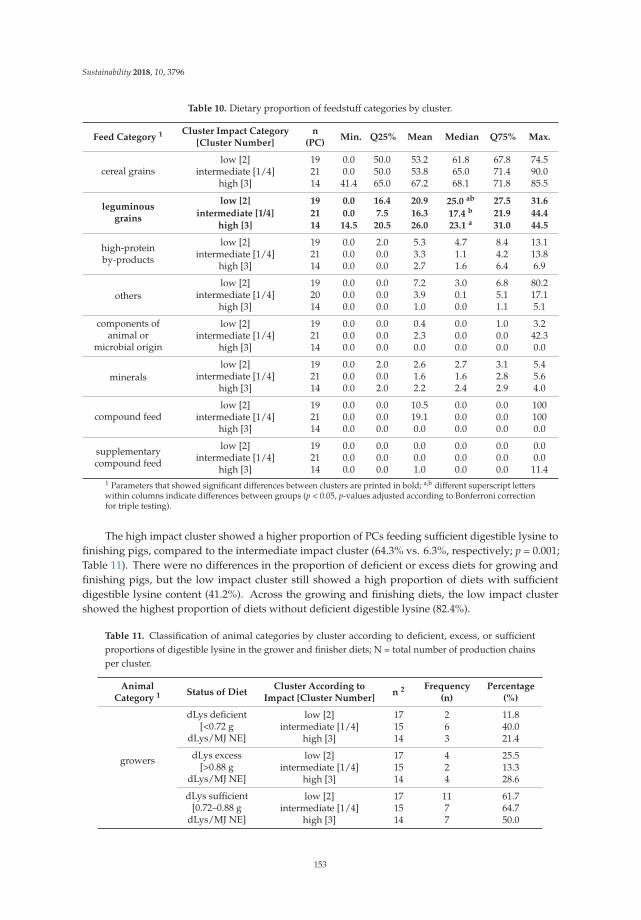
Sustainability 2018, 10, 3796
Table 10. Dietary proportion of feedstuff categories by cluster.
Feed Category 1 Cluster Impact Category[Cluster Number]
n(PC)
Min. Q25% Mean Median Q75% Max.
cereal grainslow [2] 19 0.0 50.0 53.2 61.8 67.8 74.5
intermediate [1/4] 21 0.0 50.0 53.8 65.0 71.4 90.0high [3] 14 41.4 65.0 67.2 68.1 71.8 85.5
leguminousgrains
low [2] 19 0.0 16.4 20.9 25.0 ab 27.5 31.6
intermediate [1/4] 21 0.0 7.5 16.3 17.4 b 21.9 44.4
high [3] 14 14.5 20.5 26.0 23.1 a 31.0 44.5
high-proteinby-products
low [2] 19 0.0 2.0 5.3 4.7 8.4 13.1intermediate [1/4] 21 0.0 0.0 3.3 1.1 4.2 13.8
high [3] 14 0.0 0.0 2.7 1.6 6.4 6.9
otherslow [2] 19 0.0 0.0 7.2 3.0 6.8 80.2
intermediate [1/4] 20 0.0 0.0 3.9 0.1 5.1 17.1high [3] 14 0.0 0.0 1.0 0.0 1.1 5.1
components ofanimal or
microbial origin
low [2] 19 0.0 0.0 0.4 0.0 1.0 3.2intermediate [1/4] 21 0.0 0.0 2.3 0.0 0.0 42.3
high [3] 14 0.0 0.0 0.0 0.0 0.0 0.0
mineralslow [2] 19 0.0 2.0 2.6 2.7 3.1 5.4
intermediate [1/4] 21 0.0 0.0 1.6 1.6 2.8 5.6high [3] 14 0.0 2.0 2.2 2.4 2.9 4.0
compound feedlow [2] 19 0.0 0.0 10.5 0.0 0.0 100
intermediate [1/4] 21 0.0 0.0 19.1 0.0 0.0 100high [3] 14 0.0 0.0 0.0 0.0 0.0 0.0
supplementarycompound feed
low [2] 19 0.0 0.0 0.0 0.0 0.0 0.0intermediate [1/4] 21 0.0 0.0 0.0 0.0 0.0 0.0
high [3] 14 0.0 0.0 1.0 0.0 0.0 11.41 Parameters that showed significant differences between clusters are printed in bold; a,b different superscript letterswithin columns indicate differences between groups (p < 0.05, p-values adjusted according to Bonferroni correctionfor triple testing).
The high impact cluster showed a higher proportion of PCs feeding sufficient digestible lysine tofinishing pigs, compared to the intermediate impact cluster (64.3% vs. 6.3%, respectively; p = 0.001;Table 11). There were no differences in the proportion of deficient or excess diets for growing andfinishing pigs, but the low impact cluster still showed a high proportion of diets with sufficientdigestible lysine content (41.2%). Across the growing and finishing diets, the low impact clustershowed the highest proportion of diets without deficient digestible lysine (82.4%).
Table 11. Classification of animal categories by cluster according to deficient, excess, or sufficientproportions of digestible lysine in the grower and finisher diets; N = total number of production chainsper cluster.
AnimalCategory 1 Status of Diet
Cluster According toImpact [Cluster Number]
n 2 Frequency(n)
Percentage(%)
growers
dLys deficient[<0.72 g
dLys/MJ NE]
low [2] 17 2 11.8intermediate [1/4] 15 6 40.0
high [3] 14 3 21.4
dLys excess[>0.88 g
dLys/MJ NE]
low [2] 17 4 25.5intermediate [1/4] 15 2 13.3
high [3] 14 4 28.6
dLys sufficient[0.72–0.88 g
dLys/MJ NE]
low [2] 17 11 61.7intermediate [1/4] 15 7 64.7
high [3] 14 7 50.0
153

Sustainability 2018, 10, 3796
Table 11. Cont.
AnimalCategory 1 Status of Diet
Cluster According toImpact [Cluster Number]
n 2 Frequency(n)
Percentage(%)
finishers
dLys deficient[<0.63 g
dLys/MJ NE]
low [2] 17 2 11.8intermediate [1/4] 16 7 43.8
high [3] 14 3 21.4
dLys excess[>0.77 g
dLys/MJ NE]
low [2] 17 8 47.1intermediate [1/4] 16 8 50.0
high [3] 14 2 14.3
dLys sufficient[0.63–0.77 g
dLys/MJ NE]
low [2] 17 7 41.2 ab
intermediate [1/4] 16 1 6.3 b
high [3] 14 9 64.3 a
1 Parameters that showed significant differences between clusters are printed in bold; 2 classification of diets wasnot possible for all PCs; a,b different superscript letters indicate differences between groups (p < 0.05, p-valuesadjusted according to Bonferroni correction for triple testing).
4. Discussion
4.1. General Discussion and Comparison with Other Studies
Both hypotheses were confirmed: For all environmental impact categories, variation was greaterwithin than between systems, with no distinct differences between husbandry systems regardingtheir environmental impact. Furthermore, farm characteristics contributing to environmental impactwere identified, and they were mainly related to performance (e.g., piglets weaned per sow and year,fattening pig feed conversion ratio) and feed characteristics (e.g., percentage of bought-in feed stuff infattener diets; see Section 4.2).
The selected classification was chosen according to [1], who found that specific characteristics(e.g., farm size, breeds, live-weights at slaughtering, etc.) of organic farms suggest this differentiationinto the three husbandry systems. It may be used to inform the organic sector regarding thestrengths and weaknesses of these three widely used systems’ variants, and the results may serveas a basis for system-specific mitigation strategies. The large range of results indicates potential forimprovement within all three systems. Cluster analysis was used to investigate further classification.It was interesting to find high, medium, and low impact clusters independently from husbandrysystems, but with characteristics regarding feeding and performance, which are mainly affected bymanagement decisions.
Comparing different LCA studies should always be done with caution due to differences inunderlying methodology, assumptions, and chosen system boundaries [45]. The present studyaddressed, for the first time, the environmental impact of different organic pig husbandry systemsbased on data obtained from 64 individual farrow-to-finish production chains across several Europeancountries. In accordance with [9], there was a high variation in environmental impact among farms inthe present study, indicating that individual farm characteristics highly influenced the outcome.
Other authors report comparable GWP, but rather different AP and EP (Table 12). A possiblereason is that the GWP originating from the main emission source feedstuffs does not differ widely,except for those loaded with high emissions from land use change. However, in organic systems,comparably low emissions occur from land use change. Contrarily, emission factors regarding AP andEP show a higher variation between animals kept indoors or outdoors. Additionally, methodologicaldifferences between studies (e.g., system boundaries, emission factors, type of allocation) could havecontributed to the great variation.
In general, most of our results are within the ranges reported in the literature, e.g., as provided ina review of six comparable LCA studies of pork products [4] (Table 12). The authors also found a largevariation, especially regarding acidification and eutrophication potential.
154

Sustainability 2018, 10, 3796
Our results are particularly comparable to results reported by [15], who used a similarmethodology and system boundaries for an evaluation of 15 pig farming systems from five Europeancountries. For each pig farming system, data from five to 10 farms were obtained from surveys,and systems were categorized into conventional, adapted conventional, traditional, and organic. Feedproduction contributed less to EP in organic systems than in the others [15]. In the present study,the results regarding EP (medians ranging from 20.1 to 28.7 g PO4-eq per kg live weight) exceed thevalues for organic farms found by [15]; 16 g PO4-eq), and are in the range reported for conventionalsystems. The higher EP in the present study may, on the one hand, be due to a poorer median feedconversion ratio in IN, POUT, and OUT than found by [15]. On the other hand, due to the assumptionof a 5% PO4-surplus over yield-related plant requirements, our methodological approach might haveresulted in higher PO4-emission estimates from feed production.
Regarding AP, [15] found higher medians for organic systems than for POUT and OUT in thepresent study. The even higher median AP found in IN compared to [15] may be attributed to higheremissions from manure management (storage and spreading) as well as from feed, which resultedmainly from a poorer feed conversion ratio in fatteners in the present study compared to [15].
4.2. Factors Influencing the Environmental Impacts
In terms of the relative impact of feed on GWP, AP, and EP, results presented herein agree withthose of other LCA studies [10,22,33,46,47]. Dolman et al. [9] calculated correlations between farmcharacteristics and environmental impact: All environmental indicators correlated positively withfeed intake and dietary composition. Likewise, and in accordance with [22], who identified the feedconversion ratio in fatteners as the parameter with the greatest influence on LCA outcomes, in thepresent study, the feed conversion ratio was significantly lower for fatteners in the low impact cluster.The percentage of bought-in feed for fattener diets (%) was weakly negatively correlated with AP. Thismight indicate that these feeds either were loaded with relatively low AP or the feeds contributed to abetter balanced diet and hence an improved feed conversion.
Regarding the relative contribution (%) of feedstuff categories to the environmental impactindicators, significant correlations were only found for EP. The proportion of high-protein by-productsand minerals negatively correlated with EP, while the proportion of cereal grains was positivelycorrelated. This might indicate that high-protein by-products and minerals contribute to a betterbalanced diet. Furthermore, for fed by-products, a relatively low proportion of impacts from cropproduction and processing is allocated to the co-product feed (e.g., molasses or oil cakes), and a ratherhigh share to the main product, e.g., sugar or oil.
The average fattener carcass weight (kg) was positively correlated with AP and EP, as duringthe fattening stage a large proportion of emissions arise. Towards the end of the fattening period theamount of feed needed for 1 kg of weight gain increases in comparison to earlier growing stages [42].
Furthermore, reproductive performance, especially the number of piglets born alive per litter,has been described as an important influencing factor [23,48]. However, as for all associations foundin the present study, only weak correlations regarding sow fertility and the environmental impactswere found. The number of total born (still and live born) piglets per litter negatively correlatedwith EP. However, the correlation coefficient again indicated only a weak relationship, therefore,the results do not allow for strong conclusions. Emissions originating from the sows are allocated totheir offspring, and, therefore, higher litter sizes may be regarded as beneficial if all piglets survive andgrow adequately. However, in light of the effect of litter size on piglet mortality [20], the focus shouldbe on an adequate litter size, with robust and viable piglets. This suggestion fits to the number ofpiglets weaned per sow and year being negatively associated with all environmental impact indicators,which may indicate that farms with good management and productivity are at an advantage.
155

Sustainability 2018, 10, 3796
Table 12. Greenhouse gas emissions (GWP, kg CO2-eq/FU), acidification potential (AP, g SO2-eq/FU),and eutrophication potential (EP, g PO4-eq/FU) from selected LCA studies on pig production (FU =Functional unit).
Source System/Study Case FU GWP AP EP
present results IN (indoor) kg live weight 2.2 61.9 21.6present results POUT (partly outdoor) kg live weight 2.2 51.9 20.1present results OUT (outdoor) kg live weight 2.2 55.4 28.7
[4] literature review: range across differentconventional systems kg pork 3.9–10 43–741 up to 20
[49] organic (outdoors) kg live weight 4.0 92.8 4.1
[15] range across conventional, adaptedconventional, traditional, organic kg live weight 2.2–3.4 44-57 16–34
[15] organic kg live weight 2.4 57 16[24] 1,2 conventional, base scenario kg live weight 2.4 44.8 16.1
[10] good agricultural practice kg live weight 2.3 21 44[10] ‘Label Rouge’ kg live weight 3.5 23 17
1 Results were recalculated to the functional unit of 1 kg of live weight by using the carcass yield mentioned in thestudies; 2 recalculated excluding the slaughter process.
Two farm characteristics describing the size of the pig units (number of slaughtered pigs, livestockunits per PC) negatively correlated with AP and EP, with larger PCs having lower AP and EP.The current number of sows per PC was also weakly negatively correlated with AP, in line withthe results for other farm size-related characteristics. These results may indicate that larger farms whoare more efficient in managing their pigs, eventually connected with better trained farm staff. Similarly,negative correlations were found between the average number of fattening pigs and environmentalimpact indicators in [9], but this relationship is not considered as causal and may have been related topotentially better management in larger farms.
4.3. Limitations of the Method and Uncertainties
The present study used primary data from a non-representative sample of farms instead ofmodelled data based on assumptions. Therefore, sensitivity analyses, which are used for specificscenarios, were not applied here. Besides the influence of the PC-specific characteristics, LCA resultsdepend on underlying methodological assumptions (e.g., emission factors for different floor types,allocation approach [49]). The degree of uncertainty for estimates revealed from these assumptionsmight vary between PCs, and estimates may therefore not be fully appropriate for the diversehusbandry systems in organic pig farming. A Monte Carlo analysis for the calculation of uncertaintiesof primary data as well as emission factors, describing the uncertainty areas of GWP, AP, and EPresults, was not applied in the present study. In future studies on organic pig production, an analysisof the uncertainties with data from a representative sample of farms should be implemented. Inaddition, expanded system boundaries (including, for instance, the impacts of infrastructure) shouldbe considered in future studies.
In case of emissions from feed production, uncertainty also arises from the fact that all countries’estimates were based on data for organic feed production in Austria. This approach was considered asthe best option, as comprehensive region-specific data for the production of organic feedstuffs is notavailable and calculations of these would have been beyond the project resources.
Furthermore, farm-specific primary data, such as the feed conversion ratio, may be a source ofuncertainty. The calculation of the feed conversion ratio is based on feed use (kg feed fed per day) asreported by the farmers; losses of feed, occurring especially outdoors, were probably not taken intoconsideration by some farmers. Therefore, the calculated feed conversion ratio might be higher (i.e.,poorer) than the true feed conversion ratio. However, in terms of environmental impact, the amount offeed should include feed losses.
156

Sustainability 2018, 10, 3796
These limitations offer possible improvements for future studies. As the limitations concern allhusbandry systems, they are not expected to affect the analysis of differences between husbandrysystems. Furthermore, LCA takes numerous aspects into account; if weaknesses concern single aspects,this does not reduce the meaningfulness of the calculation. Finally, it must be mentioned that, despitethese limitations, the data available for the present PC-specific cradle-to-farm gate LCA with a highnumber of organic pig farms included and taking different husbandry systems into account are unique.
5. Conclusions
Regarding environmental impact, a substantial variation was found between individual PCs. Theranking of the husbandry systems was not consistent regarding environmental impact; whereas the(median) GWP was similar in all systems; POUT had less AP than IN, and less EP than OUT.
The huge variation among PCs indicates that LCAs based on mean values of model scenarioswill not necessarily be representative for individual farms, which may be subsumed in the modelledscenario. This reflects the importance of farm specific cradle-to-farm-gate assessments, rather thangeneralized scenarios for identifying the extent and the main sources of environmental impact in thedifferent husbandry systems (IN, POUT, OUT).
In all husbandry systems, PCs with low environmental impacts were found, indicating that INand POUT as well as OUT may be managed in an environmentally friendly way. However, a lack ofconsistent differences between husbandry systems, as well as results from cluster analysis, indicate thatfactors other than the husbandry systems affect the environmental impact of organic pig production.
Feeds generally constitute an important source for environmental impact, with the feed conversionratio of fattening pigs being particularly important. Based on cluster analysis, an appropriate dietarydigestible lysine content as well as buying in feedstuffs for supplementation of protein or mineralsappears to be beneficial for a low environmental impact.
Furthermore, manure management (storage and spreading) was identified as a main source ofemissions. Measures, such as covering slurry tanks and direct application of manure to the soil, offermitigation options.
The results indicate that an overall good farm management and adequate productivity reducesthe environmental impacts, and hence optimization of management should be the focus irrespective ofthe production system.
Supplementary Materials: The following are available online at http://www.mdpi.com/2071-1050/10/10/3796/s1,Equation S1: P-losses into water bodies, Table S1: Emission factors for NH3, N2O, N2 and NO3 in outdoorpaddocks, Table S2: Emission factors for housing and manure management systems depending on floor type andmanure type, litter quality, storage period, spreading according to Rigolot et al. [29], Table S3: Characteristics of theanimal production stages by system, Table S4: Characteristics of dietary nutrient content and feed consumptionby system. The values reflect an average dietary content over all diets fed to the animal group. FCR = Feedconversion rate, n = Number of production chains, Table S5: Percentages of floor type for lactating and pregnantsows, weaners and fattening pigs kept in the systems indoor (IN) and partly outdoor (POUT), Table S6: Type andfrequency of manure treatment by system, Table S7: Cluster characteristics regarding number of sows on PC atfarm visit, average number of slaughtered fattening pigs/year and number of livestock units (LSU).
Author Contributions: G.R. provided a draft manuscript, which was revised and edited by S.H., S.E., C.W. andC.L., G.B., J.Y.D., W.Z. additionally reviewed advanced versions of the manuscript. All authors approved the finalversion of the manuscript. G.R., D.B., R.B., B.F. and A.P. collected data. G.R., S.H., G.B., R.B., J.Y.D., M.M. andW.Z. developed the methodological approach and conducted the analysis; J.Y.D. and S.H. provided the software.Conceptualization and funding acquisition of the project included D.B., S.D., J.Y.D., S.E., B.F., M.M., A.P. and C.L.
Funding: This research was funded by the FP7 ERA-Net, CORE Organic II project “ProPIG”, i.e. the nationalCORE Organic II funding agencies of Austria, Switzerland, United Kingdom, Italy, France, Denmark, Germany,Czech Republic.
Acknowledgments: The authors would like to thank all involved farmers and the ProPIG partners Tine Rousing,University of Aarhus in Denmark and Gudrun Illmann, Czech University of Life Sciences Prague.
Conflicts of Interest: The authors declare no conflict of interest.
157

Sustainability 2018, 10, 3796
References
1. Früh, B.; Bochicchio, D.; Edwards, S.; Hegelund, L.; Leeb, C.; Sundrum, A.; Werne, S.; Wiberg, S.; Prunier, A.Description of organic pig production in Europe. Org. Agric. 2014, 4, 83–92. [CrossRef]
2. Lernoud, J.; Willer, H. Current statistics on organic agriculture worldwide: Organic area, producers,markets and selected crops. In The World of Organic Agriculture. Statistics and Emerging Trends 2015;Willer, H., Lernoud, J., Eds.; IFOAM: Bonn, Germany; FiBL: Frick, Switzerland, 2015; pp. 32–116. ISBN978-3-03736-271-6.
3. Goodland, R. Livestock and Climate Change: What if the Key Actors in Climate Change Are... Cows, Pigs andChicken? Worldwatch Institute: Washington, DC, USA, 2009.
4. De Vries, M.; de Boer, I.J.M. Comparing environmental impacts for livestock products: A review of life cycleassessments. Livest. Sci. 2010, 128, 1–11. [CrossRef]
5. Gerber, P.J.; Steinfeld, H.; Henderson, B.; Mottet, A.; Opio, C.; Dijkman, J.; Falcucci, A.; Tempio, G. TacklingClimate Change through Livestock—A Global Assessment of Emissions and Mitigation Opportunities; Food andAgriculture Organization of the United Nations: Rome, Italy, 2013.
6. Jacques, S. Science and animal welfare in France and European Union: Rules, constraints, achievements.Meat Sci. 2014, 98, 484–489. [CrossRef] [PubMed]
7. FAO. SAFA Sustainability Assessment of Food and Agriculture Systems Guidelines Version 3.0; Food andAgriculture Organization of the United Nations: Rome, Italy, 2014.
8. Guinée, J.B.; Gorrée, M.; Heijungs, R.; Huppes, G.; Kleijn, R.; Koning, A.; de Oers, L.; van WegenerSleeswijk, A.; Suh, S.; Udo de Haes, H.A.; et al. Handbook on Life Cycle Assessment. Operational Guide to the ISOStandards; Kluwer Academic Publishers: Dordrecht, The Netherlands, 2002.
9. Dolman, M.A.; Vrolijk, H.C.J.; de Boer, I.J.M. Exploring variation in economic, environmental and societalperformance among Dutch fattening pig farms. Livest. Sci. 2012, 149, 143–154. [CrossRef]
10. Basset-Mens, C.; van der Werf, H.M.G. Scenario-based environmental assessment of farming systems:The case of pig production in France. Agric. Ecosyst. Environ. 2005, 105, 127–144. [CrossRef]
11. Halberg, N.; Hermansen, J.E.; Kristensen, I.S.; Eriksen, J.; Tvedegaard, N.; Petersen, B.M. Impact of organicpig production systems on CO2 emission, C sequestration and nitrate pollution. Agron. Sustain. Dev. 2010,30, 721–731. [CrossRef]
12. Olea, R.; Guy, J.; Edge, H.; Stockdale, E.A.; Edwards, S.A. Pigmeat supply chain: Life Cycle Analysis ofcontrasting pig farming scenarios. Asp. Appl. Biol. 2009, 95, 91–96.
13. Williams, A.G.; Audsley, E.; Sandars, D.L. Determining the Environmental Burdens and Resource Use in theProduction of Agricultural and Horticultural Commodities; Main Report. Defra Research Project IS0205; CranfieldUniversity and Defra: Bedford, UK, 2006.
14. Jakobsen, M.; Preda, T.; Kongsted, A.; Hermansen, J. Increased Foraging in Outdoor Organic PigProduction—Modeling Environmental Consequences. Foods 2015, 4, 622–644. [CrossRef] [PubMed]
15. Dourmad, J.Y.; Ryschawy, J.; Trousson, T.; Bonneau, M.; Gonzàlez, J.; Houwers, H.W.J.; Hviid, M.; Zimmer, C.;Nguyen, T.L.T.; Morgensen, L. Evaluating environmental impacts of contrasting pig farming systems withlife cycle assessment. Animal 2014, 8, 2027–2037. [CrossRef] [PubMed]
16. IFOAM. The IFOAM Norms for Organic Production and Processing Version 2014; IFOAM: Bonn, Germany, 2014;ISBN 978-3-944372-10-5.
17. Algers, B.; Blokhuis, H.J.; Bøtner, A.; Broom, D.M.; Costa, P.; Domingo, M.; Greiner, M.; Hartung, J.;Koenen, F.; Müller-Graf, C.; et al. Scientific opinion of the Panel on Animal Health and Welfare on a requestfrom the European Commission on species-specific welfare aspects of the main systems of stunning andkilling of farmed carp. EFSA J. 2009, 1013. [CrossRef]
18. The European Parliament and the Council of the European Union. Regulation (EU) 2018/848 of the EuropeanParliament and of the Council of 30 May 2018 on Organic Production and Labelling of Organic Products; TheEuropean Parliament and the Council of the European Union: Brussels, Belgium, 2018.
19. Edwards, S.A.; Prunier, A.; Bonde, M.; Stockdale, E.A. Special issue—Organic pig production inEurope—Animal health, welfare and production challenges. Org. Agric. 2014, 4, 79–81. [CrossRef]
20. Prunier, A.; Dippel, S.; Bochicchio, D.; Edwards, S.; Leeb, C.; Lindgren, K.; Sundrum, A.; Dietze, K.; Bonde, M.Characteristics of organic pig farms in selected European countries and their possible influence on litter sizeand piglet mortality. Org. Agric. 2014, 4, 163–173. [CrossRef]
158

Sustainability 2018, 10, 3796
21. Eriksen, J.; Hermansen, J.E.; Strudsholm, K.; Kristensen, K. Potential loss of nutrients from different rearingstrategies for fattening pigs on pasture. Soil Use Manag. 2006, 22, 256–266. [CrossRef]
22. Reckmann, K.; Krieter, J. Environmental impacts of the pork supply chain with regard to farm performance.J. Agric. Sci. 2015, 153, 411–421. [CrossRef]
23. Garcia-Launay, F.; van der Werf, H.M.G.; Nguyen, T.T.H.; Le Tutour, L.; Dourmad, J.Y. Evaluation of theenvironmental implications of the incorporation of feed-use amino acids in pig production using Life CycleAssessment. Livest. Sci. 2014, 161, 158–175. [CrossRef]
24. Nguyen, T.L.T.; Hermansen, J.E.; Mogensen, L. Fossil energy and GHG saving potentials of pig farming inthe EU. Energy Policy 2010, 38, 2561–2571. [CrossRef]
25. The British Standards Institution. Publicly Available Specification. PAS 2050: 2011 Specification for the Assessmentof the Life Cycle Greenhouse Gas Emissions of Goods and Services; British Standards Institution: London, UK, 2011.
26. Jespersen, L.M.; Baggesen, D.L.; Fog, E.; Halsnæs, K.; Hermansen, J.E.; Andreasen, L.; Strandberg, B.;Sørensen, J.T.; Halberg, N. Contribution of organic farming to public goods in Denmark. Org. Agric. 2017, 7,243–266. [CrossRef]
27. Kool, A.; Blonk, H.; Ponsioen, T.; Sukkel, W.; Vermeer, H.M.; De Vries, J.W.; Hoste, R. Carbon Footprints ofConventional and Organic Pork: Assessment of Typical Production Systems in the Netherlands, Denmark, Englandand Germany; Wageingen UR: Wageningen, The Netherlands, 2009.
28. IPCC. Guidelines for National Greenhouse Gas Inventories; Eggleston Buendia, L., Miwa, K., Ngara, T.,Tanabe, K.S., Eds.; IPCC: Geneva, Switzerland, 2006.
29. Rigolot, C.; Espagnol, S.; Pomar, C.; Dourmad, J.Y. Modelling of manure production by pigs and NH3, N2Oand CH4 emissions. Part I: Animal excretion and enteric CH4, effect of feeding and performance. Animal2010, 4, 1401–1412. [CrossRef] [PubMed]
30. Wenzel, H.; Hausschild, M.; Alting, L. Environmental Assessment of Products: Methodology, Tools and CaseStudies in Product Development; Chapman & Hall: London, UK, 1997; Volume 1.
31. Nemecek, T.; Kägi, T. Life Cyce Inventories of Swiss and European Agricultural Production Systems; Final ReportEcoinvent Report v2.0., No. 15; Agroscope Reckenholz-Taenikon: Zürich and Dübendorf, Switzerland, 2007.
32. Brandhofer, R. Umweltwirkungen Biologischer Schweinehaltung: Vergleich Zweier Haltungssysteme aufBasis des Treibhausgas-Potenzials Sowie Einer Stickstoff und Phosphorbilanz. Master’s Thesis, University ofNatural Resources and Life Sciences, Vienna, Austria, 2014.
33. Basset-Mens, C.; van der Werf, H.M.G.; Robin, P.; Morvan, T.; Hassouna, M.; Paillat, J.M.; Vertès, F. Methodsand data for the environmental inventory of contrasting pig production systems. J. Clean. Prod. 2007, 15,1395–1405. [CrossRef]
34. Dourmad, J.Y.; Physiology of Adaptation, Animal Nutrition and Health, INRA, Saint-Gilles, France. Personalcommunication, 2013.
35. Hörtenhuber, S.; Lindenthal, T.; Amon, B.; Markut, T.; Kirner, L.; Zollitsch, W. Greenhouse gas emissionsfrom selected Austrian dairy production systems—Model calculations considering the effects of land usechange. Renew. Agric. Food Syst. 2010, 25, 316–329. [CrossRef]
36. Hörtenhuber, S.J.; Lindenthal, T.; Zollitsch, W. Reduction of greenhouse gas emissions from feed supplychains by utilizing regionally produced protein sources: The case of Austrian dairy production. J. Sci.Food Agric. 2011, 91, 1118–1127. [CrossRef] [PubMed]
37. Kolbe, H. Wasserbelastung in Abhängigkeit von der Landnutzung. Available online: http://orgprints.org/801/ (accessed on 19 October 2018).
38. Samuel-Fitwi, B.; Meyer, S.; Reckmann, K.; Schroeder, J.P.; Schulz, C. Aspiring for environmentally consciousaquafeed: Comparative LCA of aquafeed manufacturing using different protein sources. J. Clean. Prod. 2013,52, 225–233. [CrossRef]
39. LCA Food database. Aalborg University and 2.-0 LCAconsultants. 2007. Available online: http://www.lcafood.dk/ (accessed on 19 Oct 2018).
40. Leeb, C.; Bernardi, F.; Winckler, C. Einführung und Monitoring von BetriebsEntwicklungsPlänen (BEP)Tiergesundheit und Wohlbefinden in Österreichischen Bioschweinebetrieben; Institut für Nutztierwissenschaften:Vienna, Austria, 2010.
41. Bayern, L. Schweinefütterung am Ökobetrieb II—Fütterungsversuche, Fütterungsempfehlungen; LfL Bayern: Poing,Germany, 2011.
159
Sustainability 2018, 10, 3796
42. Kirchgessner, M.; Roth, F.X.; Schwarz, F.J.; Stangl, G. Tierernährung. Leitfaden für Studium, Beratung und Praxis,13th ed.; DLG Verlag: Frankfurt, Germany, 2011.
43. EvaPig®. A Calculator of Energy, Amino Acid and Phosphorus Values of Ingredients and Diets for Growingand Adult Pigs. Available online: http://www.evapig.com (accessed on 19 October 2018).
44. Alibert, L. Besoins Alimentaires des Animaux en Fonction du Stade Physiologique. Available online:http://www.itab.asso.fr/downloads/porc-bio/cahier_porc_0.pdf (accessed on 10 Dec 2014).
45. Lammers, P.J. Life-cycle assessment of farrow-to-finish pig production systems: A review. CAB Rev. Perspect.Agric. Vet. Sci. Nutr. Nat. Resour. 2011, 6, 1–8. [CrossRef]
46. Pelletier, N.; Lammers, P.; Stender, D.; Pirog, R. Life cycle assessment of high- and low-profitabilitycommodity and deep-bedded niche swine production systems in the Upper Midwestern United States.Agric. Syst. 2010, 103, 599–608. [CrossRef]
47. Alig, M.; Grandl, F.; Mieleitner, J.; Nemecek, T.; Gaillard, G. Life Cycle Assessment of Beef, Pork and Poultry;Executive Summary; Reckenholz-Tänikon: Zürich, Switzerland, 2012.
48. Dalgaard, R.; Halberg, N.; Hermansen, J.E. Danish Pork Production—An Environmental Assessment; Universityof Aarhus: Tjele, Denmark, 2007; Volume 82.
49. Mackenzie, S.G.; Leinonen, I.; Ferguson, N.; Kyriazakis, I. Accounting for uncertainty in the quantification ofthe environmental impacts of Canadian pig farming systems Supplementary Material. J. Anim. Sci. 2015, 93,3130–3143. [CrossRef] [PubMed]
© 2018 by the authors. Licensee MDPI, Basel, Switzerland. This article is an open accessarticle distributed under the terms and conditions of the Creative Commons Attribution(CC BY) license (http://creativecommons.org/licenses/by/4.0/).
160

sustainability
Article
Effects of Alternative Uses of Distillery By-Productson the Greenhouse Gas Emissions of Scottish MaltWhisky Production: A System Expansion Approach
Ilkka Leinonen 1,*, Michael MacLeod 1 and Julian Bell 2
1 Land Economy, Environment and Society Research Group, Scotland’s Rural College (SRUC),Peter Wilson Building, Kings Buildings, West Mains Road, Edinburgh EH9 3JG, UK;[email protected]
2 Rural Business Unit, SAC Consulting, 2 Technopole, Bush Estate, Penicuik, Midlothian EH26 0PJ, UK;[email protected]
* Correspondence: [email protected]; Tel.: +44-131-5354044
Received: 6 April 2018; Accepted: 4 May 2018; Published: 8 May 2018
Abstract: Agricultural by-products are an important component of livestock feed. In Scotland,distillery by-products are protein rich and traditionally cost competitive feed ingredients in cattleproduction. However, during recent years, distilleries in the UK (including Scotch whisky producers)have started to use the by-products also as a source of renewable energy, in order to reduce the carbonfootprint of alcohol production. In this study, a systems-based material and energy flow analysiswas performed to calculate the life-cycle greenhouse gas (GHG) emissions of whisky productionfor two scenarios where distillery by-products were used either (1) as beef cattle feed to replaceother protein sources (namely soya bean meal and rapeseed meal); or (2) as anaerobic digester (AD)feedstock in order to generate renewable energy (heat and electricity). System expansion was used toquantitatively handle the by-products in the analysis. The results show that considerable reductionsin GHG emissions could be achieved by either replacing feed crops with by-products or by using theby-products in AD plants to generate bio-energy. The biggest reductions in the GHG emissions wereachieved when by-products were used to replace soya meal in animal feed. However, the results arehighly sensitive to methodological choices, including the accounting method of the land use changeemissions arising from soya production.
Keywords: agricultural by-products; whisky production; cattle; beef; livestock feed; renewableenergy; greenhouse gas emissions
1. Introduction
Various agricultural by-products (i.e., products originating from food and drink production butnot normally used for human consumption) are widely used as part of livestock feed. They can forman important source of protein and metabolizable energy needed for animal production [1–4] and arecurrently used in production of a wide variety of livestock species [5]. For example, brewery, spiritdistillery and bio-ethanol production by-products, such as brewers’ grains, usually made from barley,wheat, maize or rice, can form a significant part of the animal diet especially in ruminant production.These products are generally favoured due to their high protein and fibre content [6–10] and inclusionof them in ruminant feed has been found to have positive effects on the animal performance [11,12].Brewers’ grains, or further processed distillery by-product “distillers dark grains with solubles” or“dried distillers grains with solubles” (DDGS), can be also used in non-ruminant production, forexample, as part of pig feed [13–17]. According to recent studies, relative high proportions of DDGScan be applied in pig diets while still maintaining acceptable level of growth performance [15,16,18].
Sustainability 2018, 10, 1473; doi:10.3390/su10051473 www.mdpi.com/journal/sustainability161
Sustainability 2018, 10, 1473
Further application of brewery and distillery by-products such as DDGS and yeast products can alsobe found in chicken industry [19–23], or even in fish production [24,25]. However, high variability inthe nutritional value of these by-products, depending for example on the variety of the cereal, harvesttime and the malting and mashing processes [10,26,27] may limit their use in non-ruminant livestockproduction where the content of certain nutrients, especially the balance of essential amino acids,can have major impact on animal performance [28]. Despite such limitations, brewery and distilleryby-products can be potentially seen as a partial replacement of soya as a protein source in livestockproduction [20,29,30]. Reducing the dependency on soya is an increasing trend in livestock systemsdue to environmental concerns related to its production. The cultivation of this crop is generallyassociated with recent land use changes, causing greenhouse gas emissions from deforestation andconversion of other land uses to arable production, resulting in loss of carbon previously stored insoil and biomass [31]. Other environmental issues associated with soya production include the loss ofbiodiversity and freshwater and groundwater contamination [32,33].
The availability and usability of agricultural by-products or co-products can vary stronglydepending on the location of production and this can also affect the distribution and profitability oflivestock industries. In agricultural production in Scotland, barley is by far the most important arablecrop species, in terms of area of cultivation, the total mass of grain production and the amount of cropprotein produced [34]. The barley grown in Scotland is used either directly for animal feed, or as a rawmaterial of alcohol (including whisky) production. The whisky distillation process utilizes only thecarbohydrates of the barley grains, so therefore the use of the remaining compounds (including protein)in livestock production has been seen as a useful way to fully utilize this important crop. As a result,the main by-products of Scottish malt whisky production, namely “draff” (unprocessed by-productof the mashing process), “pot ale” (liquid by-product of distillation) and “distillers dark grains withsolubles” (DDGS, dried and pelletized product made of draff and pot ale) are widely used as proteinrich and low-cost ingredients of livestock feed, particularly in beef and dairy cattle production. In 2012,it was estimated that a total of 346,000 t (on a dried product basis) of distillery by-products from thewhisky industry in Scotland were potentially available for use in animal feed [35]. About 60% of thisamount was consumed in Scotland. Therefore, in this specific region, whisky industry and the feed thatit provides for livestock can be considered as a significant part of the beef and dairy production chains.
Distillery by-products used as feed have been considered to have low environmental impactsand especially low embedded greenhouse gas (GHG) emissions, compared to alternative proteinsources such as rapeseed meal and imported soya [35,36]. One of the reasons for this finding is that inagricultural life cycle assessment (LCA) studies, economic allocation of the environmental burdens isgenerally applied to distribute the burdens between various co-products originating from the sameproduction process [37–39]. In this specific method, the burdens are allocated to different co-productsproportionally to their economic value [3,36]. Therefore, due to a relatively low price of the distilleryby-products such as draff, the produced alcohol is considered to be the main product with the highestshare of the environmental burdens and only a small proportion of the overall environmental impactsassociated with whisky production is allocated to by-products [35].
In addition to the traditional use of distillery by-products as livestock feed, distilleries in Scotland(and other alcohol producers in the UK) have during recent years started to use these products asa source of renewable energy. This development is partly motivated by the government subsidiesfor such energy sources due to their low embedded GHG emissions. Furthermore, the reductionof the use of fossil fuels in the production process can also provide a greener image for the whiskyindustry through reducing its carbon footprint [40]. A recent trend in this area has been to increase theuse of by-products as a feedstock of anaerobic digestion and utilize the produced biogas to generateelectricity and heat that can be directly used in the distillation process. This strategy is expected to havemultiple benefits in terms of reduction of GHG emission. For example, in addition to the renewableenergy generated in digestion, the digestate (material remaining after the anaerobic digestion process)
162

Sustainability 2018, 10, 1473
contains nutrients that can be utilized by crops and therefore can replace the use of synthetic fertilisersand reduce the greenhouse gas emissions related to production of the fertilisers [41,42].
The proposed alternative use of distillery by-products has raised some concerns amongst livestockfarmers in Scotland and elsewhere in the UK [43]. As the use as renewable energy increases, the farmersare getting worried about the future availability and cost of by-products as animal feed. However, itshould be noted that also the feed use of these by-products can be expected to have beneficial effectson greenhouse gas emissions due to reduction of the use of carbon-intensive feed ingredients. For thisreason, a systematic comparison of GHG emissions associated with alternative uses of by-products isneeded to quantify these possible effects.
The aim of this study was to carry out a systems-based analysis of the material and energy flowswithin the whisky production chain, in order to quantitatively analyse the processes associated withdistillery by-products and assess the life-cycle greenhouse gas emissions arising from the entire whiskyproduction chain, including the end use of by-products. Instead of applying an economic allocationapproach for the outputs of the distillery processes, we selected to use a system expansion method forthe by-products, specified as “expanding the product system to include the additional functions relatedto the co-products” in the ISO [44] LCA standards. Those standards also prefer the system expansionapproach over any allocation methods and suggest that allocation between co-products should beavoided when possible. The system expansion approach makes it possible to directly compare thechanges in greenhouse gas emissions when using the by-products for alternative purposes (livestockfeed, bioenergy generation) and replacing alternative commodities (protein crops grown for cattlefeed, fossil fuels used in distillation process, synthetic fertilisers used in crop production). As anoutcome, the greenhouse gas emissions can be calculated for a unit of produced alcohol while takinginto account both the burdens and benefits achieved through the end use of the by-products.
2. Materials and Methods
A systems-based material flow analysis linking the Scottish malt whisky production and theend use of its by-products either in a cattle production system or in energy generation processeswas carried out (Figure 1) to quantify the life-cycle GHG emissions arising from whisky production.The analysis applied a system expansion approach, that is, whisky was considered as the mainproduct of distilleries, the by-products of the process were used to replace alternative commoditiesand the changes in greenhouse gas emissions as a result of this replacement were accounted forwhen quantifying the overall emissions of whisky production. In order to achieve this, the whiskyproduction system was linked to other systems affected by the by-product use, namely beef cattleproduction system, crop production system and energy generation system (see detailed system diagramin Supplementary Materials). The changes in the material and energy flows within these connectedsystems were analysed and the associated GHG emissions quantified as detailed below. This approachwas used to calculate the greenhouse gas emissions for two baseline scenarios: Scenario 1: distilleryby-products were used as cattle feed to replace either soya bean meal or rapeseed meal as a proteinsource (while maintaining the nutritional quality of the feed) and Scenario 2: distillery by-productswere used as anaerobic digester (AD) feedstock in order to generate renewable energy (heat andelectricity). For both of these scenarios, the functional unit was 1 litre of pure alcohol (LPA) and thesystem boundary was from cradle to the end of the distillation process. However, instead of the whiskyproduction chain itself (which remained the same in both baseline scenarios), the main focus of thisstudy was in the effects of alternative uses of the by-products on GHG emissions in other, connectedsystems, analysed through the system expansion approach.
163

Sustainability 2018, 10, 1473
Figure 1. A simplified diagram of the production systems analysed in this study and processes affectingthe greenhouse gas (GHG) emissions. The rectangles indicate inputs or outputs and the ovals indicateprocesses. The objects with broken lines indicate replaced products or processes partly affected bythe replacement.
The greenhouse gas emissions associated with whisky production (including production,processing and transport the raw materials but excluding the by-product processing and their end use)were quantified based on data from an earlier study [35] and the changes of these emissions, as affectedby the alternative uses of the by-products, were included in the calculations. Details of the data and thecalculated GHG emissions associated with different processes within the whisky production chain canbe found in the Supplementary Materials. Following this analysis, the processing and end use of theby-products was analysed in different scenarios, the changes in the material and energy flows withinconnected systems were quantified and the resulting increases or reductions of GHG emissions wereincluded in the total emissions of the whisky production chain. For this analysis, the quantities of theprimary by-products produced per one litre of pure alcohol were obtained from the calculations byBell et al. [35] and were estimated to be 0.56 kg DM of draff and 0.36 kg DM of pot ale. In all the systemsincluded in the calculations, the changes in the emissions of carbon dioxide (CO2), methane (CH4)and nitrous oxide (N2O) were quantified and the overall greenhouse gas emissions were expressed interms of CO2 equivalent: with a 100-year timescale, where 1 kg CH4 and N2O are equivalent to 25 and298 kg CO2 respectively [45].
2.1. Scenario 1: Distillery By-Products as Livestock Feed
In this scenario, the amounts of replaced feed ingredients in livestock production were quantified,together with the resulting changes in GHG emissions associated with feed production, entericfermentation, manure management and fertiliser use in crop production. Two alternative by-productsof malt whisky distilleries were used as a protein source in cattle feed, namely draff and DDGS. Draffwas used fresh, without further processing, while DDGS was produced as a combination of draff andpot ale and additional processing (drying and pelletizing) was needed in its production. The use ofdistillery by-products was assumed to replace two alternative protein sources widely used in Scottish
164

Sustainability 2018, 10, 1473
cattle industry, namely soya bean meal and rapeseed meal. As a result, four different options in thefeed use of the by-products were considered separately:
• Scenario 1a: draff is used to replace soya bean meal (and pot ale is disposed)• Scenario 1b: draff is used to replace rapeseed meal (and pot ale is disposed)• Scenario 1c: draff and pot ale are used to produce DDGS, which is used to replace soya bean
meal, and• Scenario 1d: draff and pot ale are used to produce DDGS, which is used to replace rapeseed meal
The amounts of the replaced alternative ingredients in animal feed were quantified based ona feeding strategy according to which the digestible protein and metabolizable energy contents ofthe feed were kept unchanged for all scenarios, although the intakes of the total combustible “gross”energy and the total (digestible + non-digestible) protein (and therefore also the total nitrogen intake)could vary between feeding options. Using this approach, also the animal performance was assumedto remain unchanged (for example, the same amount of meat was always produced per unit of energyor protein fed into the beef production system) and would therefore have no effect on the greenhousegas emissions when compared between the scenarios. Because the protein content of the distilleryby-products is lower than that of the replaced soya meal or rapeseed meal, on dry matter (DM) basishigher quantities of the by-products were needed, compared to the replaced ingredients. The higherDM quantity of the by-products brought also additional energy to the feed. Therefore, other changesin the feed were also needed to achieve equal energy content. This was done in this study by reducingthe inclusion of barley grains (which are a typical source of energy in cattle feed in Scotland) when thedistillery by-products were used in the feed. Linear optimization was used (with the constraints ofequal protein and energy content) to determine the quantities of the replaced ingredients to equal 1 kgDM of the by-product for both draff and DDGS feeding scenarios.
The nutrient contents of different feed ingredients were based on the Feedipedia [46] database.Assuming unchanged digestible protein and energy intake, the nutritional data were used to quantifythe differences in the animal intake of dry matter and nutrients when either distillery by-products oralternative ingredients were used in the feed and this information was used to quantify the changes ofthe greenhouse gas emissions arising from the livestock production system (see below).
The greenhouse gas emissions of the production of the replaced feed ingredients (soya bean meal,rapeseed meal, barley) were calculated using the Scottish Agricultural Emission Model (SAEM) [47],which is based on the FAO GLEAM livestock model [48,49]. Details of SAEM can be found in theSupplementary Materials. The emissions related to land use changes (LUC) arising from SouthAmerican soya production were also included in the calculations following the FAO [48] approachand emission factors [47]. However, since there are plenty of uncertainties in the LUC emissionsand differences in the methods for accounting for those in the context of agricultural productionchains, alternative estimates of those emissions were evaluated in the sensitivity analysis (see below).The other replaced feed crops apart from soya, that is, rapeseed and barley, were assumed to beoriginated from “mature” agricultural land in the UK and therefore no LUC emissions were associatedwith those feed ingredients [50,51].
The changes in the greenhouse gas emissions arising from enteric fermentation and manuremanagement, resulting from the changes in the feed composition, were also quantified and taken intoaccount in the analysis. The calculation of these emissions was based on the intake of nitrogen andgross energy by the animal, applying the IPCC [45] Tier 2 approach and SAEM [47] emission factors(Table 1, Supplementary Materials). In this approach, the emissions of CH4 are proportional to the feedgross energy intake of the animal and the N2O and NH3 emissions are proportional to the amount ofnitrogen excretion (affected by the protein content of the animal feed intake).
165
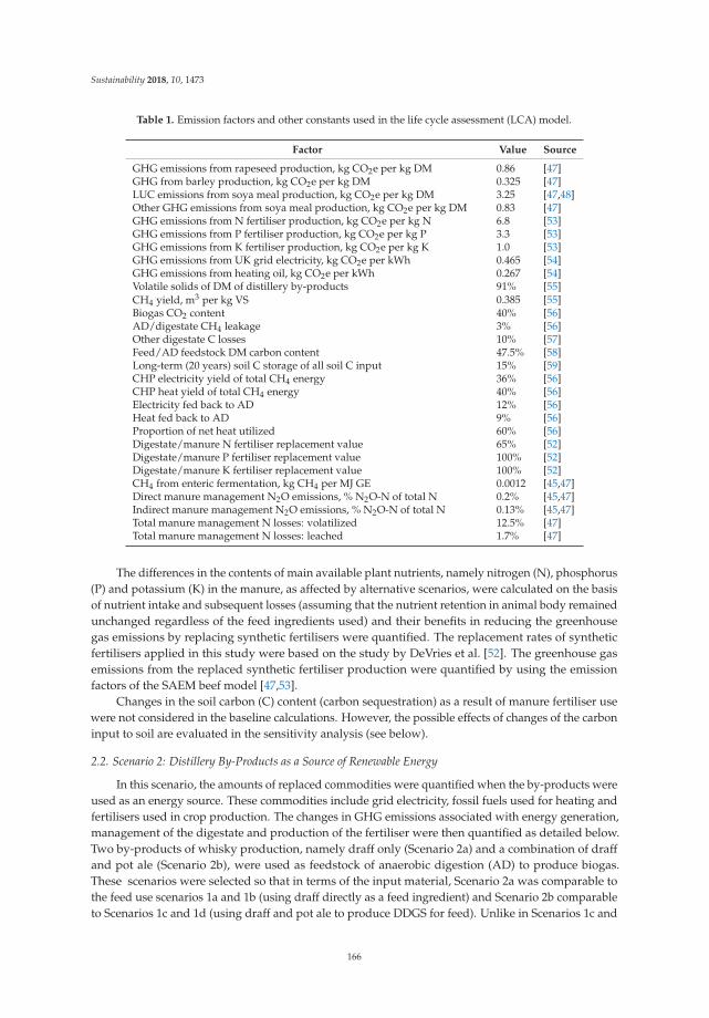
Sustainability 2018, 10, 1473
Table 1. Emission factors and other constants used in the life cycle assessment (LCA) model.
Factor Value Source
GHG emissions from rapeseed production, kg CO2e per kg DM 0.86 [47]GHG from barley production, kg CO2e per kg DM 0.325 [47]LUC emissions from soya meal production, kg CO2e per kg DM 3.25 [47,48]Other GHG emissions from soya meal production, kg CO2e per kg DM 0.83 [47]GHG emissions from N fertiliser production, kg CO2e per kg N 6.8 [53]GHG emissions from P fertiliser production, kg CO2e per kg P 3.3 [53]GHG emissions from K fertiliser production, kg CO2e per kg K 1.0 [53]GHG emissions from UK grid electricity, kg CO2e per kWh 0.465 [54]GHG emissions from heating oil, kg CO2e per kWh 0.267 [54]Volatile solids of DM of distillery by-products 91% [55]CH4 yield, m3 per kg VS 0.385 [55]Biogas CO2 content 40% [56]AD/digestate CH4 leakage 3% [56]Other digestate C losses 10% [57]Feed/AD feedstock DM carbon content 47.5% [58]Long-term (20 years) soil C storage of all soil C input 15% [59]CHP electricity yield of total CH4 energy 36% [56]CHP heat yield of total CH4 energy 40% [56]Electricity fed back to AD 12% [56]Heat fed back to AD 9% [56]Proportion of net heat utilized 60% [56]Digestate/manure N fertiliser replacement value 65% [52]Digestate/manure P fertiliser replacement value 100% [52]Digestate/manure K fertiliser replacement value 100% [52]CH4 from enteric fermentation, kg CH4 per MJ GE 0.0012 [45,47]Direct manure management N2O emissions, % N2O-N of total N 0.2% [45,47]Indirect manure management N2O emissions, % N2O-N of total N 0.13% [45,47]Total manure management N losses: volatilized 12.5% [47]Total manure management N losses: leached 1.7% [47]
The differences in the contents of main available plant nutrients, namely nitrogen (N), phosphorus(P) and potassium (K) in the manure, as affected by alternative scenarios, were calculated on the basisof nutrient intake and subsequent losses (assuming that the nutrient retention in animal body remainedunchanged regardless of the feed ingredients used) and their benefits in reducing the greenhousegas emissions by replacing synthetic fertilisers were quantified. The replacement rates of syntheticfertilisers applied in this study were based on the study by DeVries et al. [52]. The greenhouse gasemissions from the replaced synthetic fertiliser production were quantified by using the emissionfactors of the SAEM beef model [47,53].
Changes in the soil carbon (C) content (carbon sequestration) as a result of manure fertiliser usewere not considered in the baseline calculations. However, the possible effects of changes of the carboninput to soil are evaluated in the sensitivity analysis (see below).
2.2. Scenario 2: Distillery By-Products as a Source of Renewable Energy
In this scenario, the amounts of replaced commodities were quantified when the by-products wereused as an energy source. These commodities include grid electricity, fossil fuels used for heating andfertilisers used in crop production. The changes in GHG emissions associated with energy generation,management of the digestate and production of the fertiliser were then quantified as detailed below.Two by-products of whisky production, namely draff only (Scenario 2a) and a combination of draffand pot ale (Scenario 2b), were used as feedstock of anaerobic digestion (AD) to produce biogas.These scenarios were selected so that in terms of the input material, Scenario 2a was comparable tothe feed use scenarios 1a and 1b (using draff directly as a feed ingredient) and Scenario 2b comparableto Scenarios 1c and 1d (using draff and pot ale to produce DDGS for feed). Unlike in Scenarios 1c and
166

Sustainability 2018, 10, 1473
1d, no further processing of by-products (needed to produce DDGS) was applied in Scenario 2b, assuch processing would have no value in biogas production.
The produced biogas was assumed to be subsequently used to generate heat needed in mashing,fermentation and distillation processes and electricity to be fed to electrical grid, using the combinedheat and power (CHP) technology.
The yield of CH4 per kg of DM of distillery by-products was obtained fromLuna-del Risco et al. [55] and the same value was used for both Scenario 2a and 2b (Table 1).The yields of electricity and heat generated in the CHP process, the proportions of the generatedelectricity and heat needed in the AD process and efficiency of the utilization of the net heat wereobtained from an earlier study carried out at SRUC [56]. The heat obtained from the use of thebiogas was assumed to replace part of the use of fuel oil, which is a commonly used fuel in Scottishmalt whisky production as many distilleries are remote and not on the natural gas grid. Finally,the replacement of the grid electricity (i.e., the electricity fed to the grid minus the electricity usedin the AD process) and the utilizable heat (net heat production minus the heat used in the ADprocess) were quantified, the associated greenhouse gas emissions were calculated based on theUK Department for Business, Energy & Industrial Strategy emission factors [54] and these avoidedemissions were subtracted from the total greenhouse gas emissions of whisky production.
The direct and indirect greenhouse gas emissions arising from the AD and CHP processes andfrom the management of the digestate were also quantified and added to the emissions of whiskyproduction. The methane leakage was based on values from an earlier study carried out at SRUC [56]and the N2O and NH3 emissions where based on the nutrient content of the feedstock, obtained fromthe Feedipedia [46] database and calculated in a same way as the emissions from manure management.
Similarly, as in the use of the by-products as feed, the fertiliser value of the nutrients obtainedas an output of the AD process was quantified. All phosphorus and potassium of the feedstock wereassumed to remain in the digestate and the nitrogen emissions described above were subtracted fromthe total nitrogen content of the digestate. The remaining nutrients could then be expected to replacesynthetic fertilisers. It should be noted that part of the grid electricity is also generated from biomass(in 2016, this was estimated to be 7.6%, according to Ofgem [60] data) and was therefore assumed toreplace a similar amount of fertiliser per kWh of generated electricity as the AD system consideredhere. To avoid double counting, a proportion equal to this share was subtracted from the applicableorganic fertilisers produced in the AD. Similarly, as in Scenario 1, the changes in soil carbon contentwere not included in this baseline but they are evaluated in the sensitivity analysis.
A summary of the emission factors and other constants used in the calculations for differentscenarios can be found in Table 1.
2.3. Sensitivity Analysis
2.3.1. LUC Emissions
In the baseline analyses, the emissions arising from the land use changes associated with thesoya production were based on the FAO [48] default calculations methods, resulting in an emissionfactor of 3.25 kg CO2 equivalent per kg DM soya bean meal [47]. However, alternative estimatesof this value exist, so two alternatives were used here for comparison. First, recent calculations byWilliams et al. [59] estimated the direct LUC emissions to be 1.46 kg CO2e per kg DM soya bean meal(based on weighted average of the origins of soya used in the UK). Second, assuming that the soyawould originate from sustainable sources, (i.e., no LUC associated with its production) and followingthe methods of PAS 2050 carbon footprinting guidelines [50,51], the LUC emissions would be zero.
2.3.2. Carbon Sequestration
Although soil carbon content is not normally considered in agricultural LCA, changes in theecosystem carbon stock are included in the IPCC [45] guidelines for calculating GHG emissions.
167

Sustainability 2018, 10, 1473
For this reason, alternative calculations were carried out where the changes of soil carbon contentin different scenarios were estimated. First, the amount of carbon in the digestate was determinedbased on the carbon content of the AD feedstock [58] and the carbon losses as CO2 and CH4 duringthe digestion process. For the animal feed, it was assumed that the dry matter excretion rate isinversely proportional to the organic matter digestibility, obtained from the Feedipedia [46] databaseand a constant carbon content of the excreted organic matter was used in the calculations [58]. Then,the changes of the carbon input entering soil (in the fertiliser use of digestate or manure) werequantified in each scenario. Finally, following the method introduced by Williams et al. [59] andassuming the same decomposition rate of organic matter as in their study, the proportion of thecarbon remaining in the soil within a 20-year time scale (consistent with the IPCC [45] guidelines) wasdetermined to be 15% of the total addition of carbon to soil. This was then converted to avoided CO2
emissions and subtracted from the greenhouse gas emissions of whisky.
3. Results and Discussion
The potential of the distillery by-products to replace different feed ingredients in either soya mealbased (Scenarios 1a and 1c) or rapeseed meal based (Scenarios 1b and 1c) feed is presented in Table 2.The results show that using an equal amount of the by-product, generally a bigger amount of rapeseedmeal could be replaced than soya bean meal, due to the lower protein content of the former. It canbe also seen that on the dry matter basis, DDGS is more efficient than draff in replacing alternativeprotein sources.
Table 2. The amounts of different feed ingredients in cattle feed replaced by the distillery by-products(Draff or dried distillers grains with solubles (DDGS)) in different scenarios. The quantities are basedon equal content of metabolizable energy and digestible protein.
By-Product (1 kg DM) Replaced Soya Meal, kg DM Replaced Rapeseed Meal, kg DM Replaced Barley, kg DM
Draff: Scenario 1a 0.28 0.41Draff: Scenario 1b 0.44 0.32DDGS: Scenario 1c 0.39 0.54DDGS: Scenario 1d 0.60 0.42
Replacement of alternative feed ingredients resulted in considerable reductions in greenhousegas emissions arising from feed production (Table 3). When comparing different alternative proteinsources (soya and rapeseed), higher reductions could be achieved when soya bean meal was removedfrom the feed, due to avoided emissions that would arise from land use changes associated withsoya production.
Table 3. Effects of replacing soya bean meal or rapeseed meal in cattle feed by distillery by-products(Draff or DDGS) on GHG emissions arising from different sources (kg CO2 equivalent per 1 kg DM ofby-product). Negative signs indicate reduction of emissions and positive signs increase of emissions.
Source of GHG EmissionDraff Replacing
Soya (Scenario 1a)Draff Replacing
Rapeseed (Scenario 1b)DDGS ReplacingSoya (Scenario 1c)
DDGS ReplacingRapeseed (Scenario 1d)
Feed production −1.288 −0.480 −1.773 −0.655Manure N2O 0.002 −0.001 0.003 −0.001
CH4 enteric fermentation 0.063 0.049 0.14 0.066N fertiliser replacement −0.005 0.001 −0.007 0.001P fertiliser replacement 0.001 −0.005 −0.016 −0.024K fertiliser replacement 0.009 0.002 0.002 −0.007
Processing (DDGS) 0 0 0.518 0.518
Total −1.219 −0.433 −1.133 −0.101
There were only minor changes in emissions directly related to livestock production, other thanthose arising from feed production, when distillery by-products were replaced with alternative feed
168

Sustainability 2018, 10, 1473
ingredients (Table 3). The reason for that is that the inputs (gross energy intake, nutrient intake)affecting those emissions in the calculations based on IPCC Tier 2 method remained very similar in allfeeding scenarios. This is expected, as the quantities of the feed ingredients consumed by the animalswere specified so that the metabolizable energy intake and the digestible protein intake (affecting Nemissions) remained constant in all scenarios. The differences in those emissions were thus a result ofsmall differences in the contents of nutrients in the feed and different digestibility of energy and proteinin different feed ingredients. These factors affected the avoided emissions related to the production ofreplaced fertilisers but the differences in those emissions were also rather small between the feedingscenarios with different feed ingredients.
The outputs of the scenario where the distillery by-products were used to generate renewableenergy are presented in Table 4. In addition to the generated electricity and heat (replacing gridelectricity and heating oil used in whisky production), considerable amounts of synthetic fertiliserscould also be replaced when the digestate obtained from the anaerobic digestion would be used as afertiliser in crop production.
Table 4. Outputs of use of distillery by-products as a source of renewable energy by applying acombination of anaerobic digester (AD) and combined heat and power (CHP) (per 1 kg of dry matter(DM) of the by-product).
Outputs per 1 kg DM by-Product Draff (Scenario 2a) Draff + Pot Ale (Scenario 2b)
Methane, m3 0.351 0.351Electricity to grid, kWh 1.146 1.146
Utilized heat, kWh (replacing oil) 0.790 0.790Replaced N as fertiliser, kg 0.018 0.024Replaced P as fertiliser, kg 0.003 0.009Replaced K as fertiliser, kg 0.0003 0.009
Since the same conversion factor for methane yield was used for different types of distilleryby-products when used as AD feedstock [55], there were no differences in the amount of energygenerated per unit of DM between the options where draff only or a combination of draff and pot alewere used in AD. However, there were differences in the amount of fertiliser that could be replaced bythe digestate, depending on the feedstock used. This was due to the high nutrient content of pot aleand for this reason, the digestate from the combination of draff and pot ale had a higher capacity toreplace fertilisers than the digestate originating from draff only.
The biggest part of the reductions in the greenhouse gas emissions, when distillery by-productswere used as AD feedstock, was associated with the replaced grid electricity (Table 5). However,considerable reductions were achieved also by using the digestate to replace synthetic fertilisers, mostnotably nitrogen fertilisers. Unlike in the Scenario 1, most of the nutrients entering to the AD processas part of the feedstock could actually be credited to whisky production. In contrast, in the feed use,the difference in the nutrient output between the by-products and the alternative feed ingredients wasrather small. The reduction of the GHG emissions was also affected by the emissions of methane andnitrous oxide arising from the digestion process and storage of the digestate (Table 5).
169
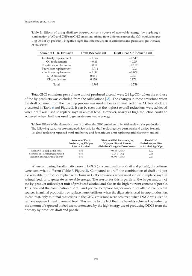
Sustainability 2018, 10, 1473
Table 5. Effects of using distillery by-products as a source of renewable energy (by applying acombination of AD and CHP) on GHG emissions arising from different sources (kg CO2 equivalent per1 kg DM of by-product). Negative signs indicate reduction of emissions and positive signs increaseof emissions.
Source of GHG Emission Draff (Scenario 2a) Draff + Pot Ale (Scenario 2b)
Electricity replacement −0.549 −0.549Oil replacement −0.25 −0.25
N fertiliser replacement −0.12 −0.159P fertiliser replacement −0.011 −0.03K fertiliser replacement −0.000 −0.009
N2O emissions 0.051 0.063CH4 emissions 0.176 0.176
Total −0.703 −0.759
Total GHG emissions per volume unit of produced alcohol were 2.6 kg CO2 when the end useof the by-products was excluded from the calculations [35]. The changes in these emissions whenthe draff obtained from the mashing process was used either as animal feed or as AD feedstock arepresented in Table 6 and Figure 2. It can be seen that the highest overall reductions were achievedwhen draff was used to replace soya in animal feed. However, nearly as high reduction could beachieved when draff was used to generate renewable energy.
Table 6. Effects of the alternative uses of draff on the GHG emissions of Scottish malt whisky production.The following scenarios are compared: Scenario 1a: draff replacing soya bean meal and barley, Scenario1b: draff replacing rapeseed meal and barley and Scenario 2a: draff replacing grid electricity and oil.
Amount of DraffProduced, kg DM per
Litre of Alcohol
Effect on GHG Emissions, kgCO2e per Litre of Alcohol
(Relative Change in Parentheses)
Final GHGEmissions per Litreof Alcohol, kg CO2e
Scenario 1a: Replacing soya 0.56 −0.68 (−26%) 1.92Scenario 1b: Replacing rapeseed 0.56 −0.24 (−9%) 2.36Scenario 2a: Renewable energy 0.56 −0.39 (−15%) 2.21
When comparing the alternative uses of DDGS (or a combination of draff and pot ale), the patternswere somewhat different (Table 7, Figure 2). Compared to draff, the combination of draff and potale was able to produce higher reductions in GHG emissions when used either to replace soya inanimal feed, or to generate renewable energy. The reason for this is partly in the larger amount ofthe by-product utilised per unit of produced alcohol and also in the high nutrient content of pot ale.This enabled the combination of draff and pot ale to replace higher amount of alternative proteinsources in animal production, or replace more fertilisers when the digestate is used in crop production.In contrast, only minimal reductions in the GHG emissions were achieved when DDGS was used toreplace rapeseed meal in animal feed. This is due to the fact that the benefits achieved by reducingthe amount of rapeseed in feed are counteracted by the high energy use of producing DDGS from theprimary by-products draff and pot ale.
170

Sustainability 2018, 10, 1473
Table 7. Effects of the alternative uses of combination of draff and pot ale on the GHG emissions ofScottish malt whisky production. The following scenarios are compared: Scenario 1c: DDGS replacingsoya bean meal and barley, Scenario 1d: DDGS replacing rapeseed meal and barley and Scenario 2b:draff + pot ale replacing grid electricity and oil.
Amount of Draff + PotAle Produced, kg DM
per Litre of alcohol
Effect on GHG Emissions, kgCO2e per Litre of Alcohol
(Relative Change in Parentheses)
Final GHGEmissions per Litreof Alcohol, kg CO2e
Scenario 1c: Replacing soya 0.92 −1.04 (−40%) 1.57Scenario 1d: Replacing rapeseed 0.92 −0.09 (−3%) 2.51Scenario 2b: Renewable energy 0.92 −0.70 (−27%) 1.91
Figure 2. GHG emissions of Scottish malt whisky production with different end uses of by-products.Scenarios applying draff only are presented in blue colour and scenarios applying both draff and potale in red colour. Scenario 1a: draff replacing soya bean meal and barley, Scenario 1b: draff replacingrapeseed meal and barley, Scenario 1c: DDGS replacing soya bean meal and barley, Scenario 1d: DDGSreplacing rapeseed meal and barley, Scenario 2a: draff replacing grid electricity and oil and Scenario2b: draff + pot ale replacing grid electricity and oil.
The sensitivity analysis shows that the method used for quantifying the GHG emissions associatedwith the land use changes has a major effect on the comparison between different uses of theby-products and on conclusions drawn from this comparison. It can be seen in Table 8 that whenlower LUC emissions are applied for soya, the benefits of by-product feed use in reduction of theGHG emissions are largely lost and the use of the by-products for heat and electricity generationbecomes the most efficient option. In fact, in the option where zero LUC emissions were assigned tosoya production, the use of DDGS to replace soya became the least efficient way to reduce the GHGemissions of whisky production, while in the baseline scenario it resulted in the highest reductions.
Including the carbon sequestration (i.e., changes in soil carbon content as a result of the alternativeuses of the by-products) also affected the results. In general, when such changes were accounted for,the efficiency of energy generation option in reducing the GHG emissions increased. This is becausethe net input of C to soil increases when digestate is used as a fertiliser. However, an increase insoil carbon was also observed when the by-products were used as animal feed. This increase was aresult of the lower digestibility (i.e., higher proportion of non-digestible carbon compounds per unit of
171

Sustainability 2018, 10, 1473
digestible energy) of the by-products and hence higher dry matter excretion when the by-productswere used as feed, compared to the alternative feed ingredients barley and soya/rapeseed.
Table 8. The results of the sensitivity analysis showing the GHG emissions (kg CO2e per litre of alcohol)with different assumptions of land use changes (LUC)-related emissions and carbon sequestration.Scenario 1a: draff is used to replace soya; Scenario 1b: draff is used to replace rapeseed; Scenario 1c:DDGS is used to replace soya; Scenario 1d: DDGS is used to replace rapeseed meal; Scenario 2a: draff isused to replace grid electricity and oil; Scenario 2b: draff and pot ale are used to replace grid electricityand oil.
Scenario 1a Scenario 1b Scenario 1c Scenario 1d Scenario 2a Scenario 2b
Baseline 1.92 2.36 1.57 2.51 2.21 1.91Alternative LUC emissions
(Williams et al. 2016) 2.21 2.36 2.21 2.51 2.21 1.91
No LUC emissions 2.44 2.36 2.73 2.51 2.21 1.91Including carbon sequestration 1.88 2.33 1.53 2.50 2.16 1.83
General Discussion
Overall, the results confirm the expectations of the whisky industry that the carbon footprintof whisky production can be reduced considerably when the by-products are used to generateheat and electricity and therefore the use of fossil fuels in the distillation process can be reduced.However, the by-products can also have other, indirect effects outside the distillery system, affectinggreenhouse gas emissions. To understand and quantify such effects, other systems, in addition towhisky production itself, need to be included in the analysis and this can be done by applying asystems-based modelling approach.
In general, when the greenhouse gas emissions related to agricultural by-products (or co-products)are considered using LCA or other environmental assessment methods, the methodological choicesrelated to allocation of the environmental burdens between those products often become a centralissue of the analysis. Unfortunately, such choices can be very much subjective and they can alsostrongly affect the outcomes of the study in question. In studies related to livestock production andespecially animal feeding, the use of various by-products as feed ingredients has often been foundas an environmentally friendly option [3,36]. The reason for this that amongst different potentialapproaches to handling the co-products in environmental impact assessment, economic allocationhas been widely used in agricultural LCA studies [38,39,61]. As an outcome of such analyses, smallerproportions of the environmental impacts are allocated to low value by-products, compared to the“main” product. In many cases, such an approach is justified and preferred, keeping in mind that themain product, not the by-products, is actually the driving force of the production.
Despite the general applicability of the economic allocation, alternative allocation methods havealso been suggested for agricultural LCA. The idea behind this is that the ISO [44] standards preferthe use of a “causal” or “physical” allocation method, in cases where allocation cannot be avoidedaltogether for example through system separation. Another reason for avoiding economic allocation isthe potentially varying prices of the co-products, which has sometimes been considered problematicand causing inconsistencies in LCA studies. However, alternative methods, such as system separation,or so called “biophysical allocation”, where the aim is to link the inputs to outputs through actualphysical flows or causalities [61–65] are problematic due to the unique nature of agricultural LCA.The fact is that agricultural products are always an outcome of complicated biological processeswith various interactions. Therefore, attempts to physically separate the processes behind eachco-product are not meaningful as such an approach would necessarily be based on arbitrary, subjectivedecisions [66]. In addition to attempts to model the physical flows, other “physical” allocation methods,used to avoid economic allocation, can be based for example on mass (fresh or dry matter) or proteinor energy content of the products. Again, using such methods in agricultural LCA in a systematic way
172

Sustainability 2018, 10, 1473
can be very difficult, due to potentially varying end uses of the by-products and possible difficulties indistinguishing between actual products and waste materials, for example, in case of manure [66].
To avoid allocation, in cases where system separation is not possible, the ISO [44] standardsrecommend using a system expansion approach. System expansion is also preferred over co-productallocation in various carbon footprinting guidelines such as PAS 2050 [50]. Over recent years, thisapproach has been widely applied for example in LCA studies on livestock production [67,68].However, as pointed out by Mackenzie et al. [66], the use of this approach cannot be considered asbecoming a general practice in agricultural LCA, for example due to possible difficulties in identifyingthe main product and by-products. Another difficulty with this approach is that it could requirelarge amount of additional data from other sub-processes or systems [66,69,70]. Despite possibleshortcomings, the use this method can be considered to be justified in many cases and especiallywhen 1) the process in question is clearly targeted to produce one specific main product and 2) thefocus of the analysis is in alternative uses of the emerging by-products, not in the production processitself. This was the case in this study and in fact, it would be difficult to systematically comparethe very different uses of whisky by-products by applying any other of those alternative methodsmentioned above.
The system expansion (usually as part of so called “consequential LCA” approach [71]) hasbeen earlier used in other studies evaluating the environmental consequences of alternative usesof agricultural by-products, including the use of those products in generating renewable energy.For example, Styles et al. [57] used a consequential approach to quantify the reduction of the GHGemissions when manure and food waste are used in AD in a dairy farm. Their conclusion was that theachieved benefits were dependent on how much crops were used as co-digestate in addition to themanure, as this would determine the need for animal feed imported to the farm, which had its owneffect on the feed-related GHG emissions. In another study, van Zanten et al. [72] applied consequentialLCA to compare uses of two by-products, namely wheat middlings and beet tails. In the case of thebeet tails, the alternative use also in their study was bioenergy generation using AD, as opposed tousing them as cattle feed.
Williams et al. [59] assessed the effects of alternative end uses of turkey litter on the environmentalimpacts of turkey meat production. Also in that study, a system expansion approach was used in orderto compare the use of litter either as a biofuel (used for electricity generation in a large-scale powerplant) or directly as a fertiliser through land spreading. Similarly, as in the current study, the availabilityof nutrients for crop production, obtained from the litter, was quantified for both scenarios and thedisplacement of the synthetic fertilisers (and the grid energy in the case of bioenergy use) was takeninto account when calculating the total emissions related to turkey production. That study alsodemonstrated the potentially significant effect of carbon sequestration on the overall GHG emissionsarising from agricultural production.
4. Conclusions
The most notable reductions of greenhouse gas emissions of whisky production were achievedwhen the distillery by-products replaced soya meal, the production of which is associated with landuse changes. When using the by-products to replace alternative feed ingredients, there were changesalso in emissions from enteric fermentation, manure management and the end use of manure andits potential to replace synthetic fertilisers but these had only minor effect on the overall greenhousegas emissions, compared to effect achieved by changes in the production of the feed and related LUCemissions. Different by-products had different environmental effects when used as livestock feed.Compared to draff, DDGS could reduce more greenhouse gas emissions related to production of thereplaced feed ingredients but on the other hand, it had higher emissions arising from processing,especially from drying and pelletizing.
The use of by-products as a source of renewable energy, that is, production and combustion ofbiogas, reduced the greenhouse gas emissions by replacing grid electricity and fossil fuels used for
173

Sustainability 2018, 10, 1473
heating. Additional benefits were achieved by using the digestate as a fertiliser and thus replacingthe production of synthetic nitrogen fertilisers. Overall, the energy use of by-products could producereduction of greenhouse gas emissions with similar magnitude as the use of the by-products as feed.
It should be also noted that in the case of this study, similarly as in earlier studies onagricultural by-products discussed above, the outcome is largely dependent on methodological choices.The sensitivity analysis demonstrates that the calculated reductions in the GHG emissions are stronglyaffected by the method how the emissions associated with land use changes and land management areaccounted for in the calculations. Currently, there is no generally accepted approach to this process andthis is causing difficulties in comparing the results of agricultural LCAs, especially in cases where theproducts are strongly associated with LUC. In assessment of greenhouse gas emissions in agriculturalproduction, probably the most important single product where direct LUC is involved is soya beanmeal imported from South America. This has been demonstrated for example by Leinonen et al. [51],who applied LCA modelling to quantify the environmental impacts of UK poultry production systemswith alternative scenarios using different protein crops as a basis of diet formulations for broilers andlaying hens. The general conclusion of their study was that inclusion of alternative protein sources(e.g., beans or peas) to replace soya bean meal could slightly reduce the Global Warming Potential ofbroiler and egg production but also in that study, this observed reduction was highly dependent onthe LUC emission accounting method.
A high sensitivity to the LUC emissions was also found by van Zanten et al. [72]. According totheir findings, higher reductions in GHG emissions could be achieved with the feed use of beettails, through displaced emissions related to barley production, when compared to the bioenergy use.However, this was only the case when indirect LUC emissions were accounted for in barley productions,which is not a common practice in agricultural LCA studies [73]. If these emissions were excluded,higher reductions in the emissions could be achieved through the bioenergy option [72]. To avoid thesemethodological problems, some attempts have been made to harmonize the LUC accounting methodsin agricultural LCA [73,74]. Despite this, current inconsistencies in the methods will necessarily remaina challenge in interpretation of the results of studies on environmental sustainability of agriculturalproducts, especially in the context of livestock systems.
In addition to carbon losses due to land use changes, agricultural systems can also contribute tocarbon sequestration. Although a large proportion of the carbon in the UK soils has been lost duringrecent decades, partly as a result of agricultural practices [75,76], this trend can be partially reversedfor example, by the use of organic fertilisers. Although the changes in soil carbon (other than thoserelated to land use changes) are not usually considered in agricultural LCA, we explored this processin the sensitive analysis of this study, using a similar approach as Williams et al. [59]. In general,soil carbon balance is potentially an important component of the overall effect of agricultural andbioenergy systems on global GHG emissions and therefore should not be ignored in such studies.
Supplementary Materials: The following supplementary materials are available online at http://www.mdpi.com/2071-1050/10/5/1473/s1, 1. Diagram of the production systems and material flows, 2. Quantifying GHGemissions from malt whisky production and 3. Outline of the Scottish Agricultural Emission Model (SAEM).
Author Contributions: All authors contributed to the design of the study, analysis of the data and writing thepaper. I.L. led the writing process and data analysis, M.M. led the development of the livestock modelling tooland J.B. provided unpublished data for the analysis.
Acknowledgments: This research was undertaken within the Scottish Government Rural Affairs and theEnvironment Portfolio Strategic Research Programme 2016–2021, WP 1.4 “Integrated and Sustainable Managementof Natural Assets” and 2.4 “Rural Industries.”
Conflicts of Interest: The authors declare no conflict of interest.
174

Sustainability 2018, 10, 1473
References
1. Woyengo, T.A.; Beltranena, E.; Zijlstra, R.T. Nonruminant Nutrition Symposium: Controlling feed cost byincluding alternative ingredients into pig diets: A review. J. Anim. Sci. 2014, 92, 1293–1305. [CrossRef][PubMed]
2. Zijlstra, R.T.; Beltranena, E. Swine convert co-products from food and biofuel industries into animal proteinfor food. Anim. Front. 2013, 3, 48–53. [CrossRef]
3. Mackenzie, S.G.; Leinonen, I.; Ferguson, N.; Kyriazakis, I. Can the environmental impact of pig systems bereduced by utilising co-products as feed? J. Clean. Prod. 2016, 115, 172–181. [CrossRef]
4. Nonhebel, S. Energy from agricultural residues and consequences for land requirements for food production.Agric. Syst. 2007, 94, 586–592. [CrossRef]
5. Ajila, C.M.; Brar, S.K.; Verma, M.; Tyagi, R.D.; Godbout, S.; Valéro, J.R. Bio-processing of agro-byproducts toanimal feed. Crit. Rev. Biotechnol. 2012, 32, 382–400. [CrossRef] [PubMed]
6. Dhiman, T.R.; Bingham, H.R.; Radloff, H.D. Production response of lactating cows fed dried versus wetbrewers’ grain in diets with similar dry matter content. J. Dairy Sci. 2003, 86, 2914–2921. [CrossRef]
7. Miyazawa, K.; Sultana, H.; Hirata, T.; Kanda, S.; Itabashi, H. Effect of brewer’s grain on rumen fermentation,milk production and milk composition in lactating dairy cows. Anim. Sci. J. 2007, 78, 519–526. [CrossRef]
8. Chiou, P.W.S.; Chen, C.R.; Chen, K.J.; Yu, B. Wet brewers’ grains or bean curd pomance as partial replacementof soybean meal for lactating cows. Anim. Feed Sci. Technol. 1998, 74, 123–134. [CrossRef]
9. Gallo, M.; Sommer, A.; Mlynar, R.; Rajcakova, L. Effect of dietary supplementation with brewery draff onrumen fermentation and milk production in grazing dairy cows. J. Farm. Anim. Sci. 2001, 34, 107–113.
10. Mussatto, S.I.; Dragone, G.; Roberto, I.C. Brewers’ spent grain: Generation, characteristics and potentialapplications. J. Cereal Sci. 2006, 43, 1–14. [CrossRef]
11. Belibasakis, N.G.; Tsirgogianni, D. Effects of wet brewers grains on milk yield, milk composition and bloodcomponents of dairy cows in hot weather. Anim. Feed Sci. Technol. 1996, 57, 175–181. [CrossRef]
12. Sawadogo, L.; Sepehri, H.; Houdebine, L.M. Presence of a factor stimulating prolactin and growth hormonesecretion in brewers’ spent grains. Reprod. Nutr. Dev. 1989, 29, 139–146. [CrossRef] [PubMed]
13. Yaakugh, I.D.I.; Tegbe, T.S.B.; Olorunju, S.A.S.; Aduku, A.O. Replacement value of brewers’ dried grain formaize on performance of pigs. J. Sci. Food Agric. 1994, 66, 465–471. [CrossRef]
14. Dung, N.N.X.; Manh, L.H.; Udén, P. Tropical fibre sources for pigs—Digestibility, digesta retention andestimation of fibre digestibility in vitro. Anim. Feed Sci. Technol. 2002, 102, 109–124. [CrossRef]
15. Gutierrez, N.A.; Kil, D.Y.; Liu, Y.; Pettigrew, J.E.; Stein, H.H. Effects of co-products from the corn-ethanolindustry on body composition, retention of protein, lipids and energy and on the net energy of diets fed togrowing or finishing pigs. J. Sci. Food Agric. 2014, 94, 3008–3016. [CrossRef] [PubMed]
16. Stein, H.H.; Shurson, G.C. Board-invited review: The use and application of distillers dried grains withsolubles in swine diets. J. Anim. Sci. 2009, 87, 1292–1303. [CrossRef] [PubMed]
17. Duttlinger, A.J.; Derouchey, J.M.; Tokach, M.D.; Dritz, S.S.; Goodband, R.D.; Nelssen, J.L.; Houser, T.A.;Sulabo, R.C. Effects of increasing crude glycerol and dried distillers grains with solubles on growthperformance, carcass characteristics and carcass fat quality of finishing pigs. J. Anim. Sci. 2012, 90, 840–852.[CrossRef] [PubMed]
18. Graham, A.B.; Goodband, R.D.; Tokach, M.D.; Dritz, S.S.; Derouchey, J.M.; Nitikanchana, S.; Updike, J.J. Theeffects of low-, medium- and high-oil distillers dried grains with solubles on growth performance, nutrientdigestibility and fat quality in finishing pigs. J. Anim. Sci. 2014, 92, 3610–3623. [CrossRef] [PubMed]
19. Olumu, J.M. Industrial by-products as alternative to maize in ration. Anim. Sci. J. 1988, 15, 61–63.20. Carias, D.; Millan, N. Brewery waste as a substitute for soy protein in soy-brewer’s yeast mixtures to feed
broiler chickens. Arch. Latinoam. Nutr. 1996, 46, 67–70. [PubMed]21. Onifade, A.A.; Babatunde, G.M. Comparison of the utilization of palm kernel meal, brewer’s dried grains
and maize offal by broiler chicks. Br. Poult. Sci. 1998, 39, 245–250. [CrossRef] [PubMed]22. Kratzer, F.H.; Earl, L. The feeding value of the protein of brewers’ dried grains for chicks. Poult. Sci. 1980, 59,
2361–2364. [CrossRef]23. Swain, B.K.; Naik, P.K.; Chakurkar, E.B.; Singh, N.P. Effect of feeding brewers’ dried grain on the performance
and carcass characteristics of Vanaraja chicks. J. Appl. Anim. Res. 2012, 40, 163–166. [CrossRef]
175

Sustainability 2018, 10, 1473
24. Kaur, V.I.; Saxena, P.K. Incorporation of brewery waste in supplementary feed and its impact on growth insome carps. Bioresour. Technol. 2004, 91, 101–104. [CrossRef]
25. Muzinic, L.A.; Thompson, K.R.; Morris, A.; Webster, C.D.; Rouse, D.B.; Manomaitis, L. Partial and totalreplacement of fish meal with soybean meal and brewers’ grains with yeast in practical diets for Australianred claw crayfish Cherax quadricarinatus. Aquaculture 2004, 230, 359–376. [CrossRef]
26. Huige, N.J. Brewery by-products and effluents. In Handbook of Brewing; Hardwick, W.A., Ed.; Marcel Dekker:New York, NY, USA, 1994; pp. 501–550. ISBN 9780585139173.
27. Santos, M.; Jiménez, J.J.; Bartolomé, B.; Gómez-Cordovés, C.; del Nozal, M.J. Variability of brewers’ spentgrain within a brewery. Food Chem. 2003, 80, 17–21. [CrossRef]
28. National Research Council. Nutrient Requirements of Swine, 11th ed.; The National Academies Press:Washington, DC, USA, 2012; ISBN 978-0-309-22423-9.
29. Ghazalah, A.A.; Abd-Elsamee, M.O.; Moustafa, E.S. Use of distillers dried grains with solubles (DDGS) asreplacement for soybean meal in laying hen diets. Int. J. Poult. Sci. 2011, 10, 505–513. [CrossRef]
30. Hoffman, L.A.; Baker, A. Estimating the Substitution of Distillers’ Grains for Corn and Soybean Meal inthe U.S. Feed Complex. Economic Research Service/USDA. Available online: https://www.ers.usda.gov/publications/pub-details/?pubid=36472 (accessed on 27 April 2018).
31. Guo, L.B.; Gifford, R.M. Soil carbon stocks and land use change: A meta analysis. Glob. Chang. Biol. 2002, 8,345–360. [CrossRef]
32. Soya and the Cerrado: Brazil’s Forgotten Jewel. WWF Report UK 2012. Available online: http://assets.wwf.org.uk/downloads/soya_and_the_cerrado.pdf (accessed on 27 April 2018).
33. Clay, J. World Agriculture and the Environment, 4th ed.; Island Press: Washington, DC, USA, 2003; ISBN9781559633703.
34. Economic Report on Scottish Agriculture. Available online: http://www.gov.scot/Topics/Statistics/Browse/Agriculture-Fisheries/PubEconomicReport (accessed on 26 March 2018).
35. Bell, J.; Morgan, C.; Dick, G.; Reid, G. Distillery Feed By-Products Briefing, An AA211 Special EconomicStudy for the Scottish Government. 2012. Available online: http://www.sruc.ac.uk/download/downloads/id/1057/distillery_feed_by-products_briefing (accessed on 26 March 2018).
36. Meul, M.; Ginneberge, C.; Van Middelaar, C.E.; de Boer, I.J.M.; Fremaut, D.; Haesaert, G. Carbon footprint offive pig diets using three land use change accounting methods. Livest. Sci. 2012, 149, 215–223. [CrossRef]
37. De Vries, M.; de Boer, I.J.M. Comparing environmental impacts for livestock products: A review of life cycleassessments. Livest. Sci. 2010, 128, 1–11. [CrossRef]
38. Ardente, F.; Cellura, M. Economic allocation in life cycle assessment. J. Ind. Ecol. 2012, 16, 387–398. [CrossRef]39. Brankatschk, G.; Finkbeiner, M. Application of the Cereal Unit in a new allocation procedure for agricultural
life cycle assessments. J. Clean. Prod. 2014, 73, 72–79. [CrossRef]40. Scots Whisky Association. Environmental Strategy. Available online: http://www.scotch-whisky.org.uk/
what-we-do/environmental-strategy/ (accessed on 26 March 2018).41. Risberg, K.; Cederlund, H.; Pell, M.; Arthurson, V.; Schnürer, A. Comparative characterization of digestate
versus pig slurry and cow manure—Chemical composition and effects on soil microbial activity. Waste Manag.2017, 61, 529–538. [CrossRef] [PubMed]
42. Ohdoi, K.; Miyahara, S.; Iwashita, K.; Umeda, M.; Shimizu, H.; Nakashima, H.; Miyasaka, J. Optimizationof fertiliser application schedule: Utilization of digestate after anaerobic digestion as liquid fertiliser.IFAC Proc. Vol. 2013, 46, 317–322. [CrossRef]
43. Scottish Tenant Farmers Association News Release, 21st February 2017. Available online:http://www.tfascotland.org.uk/stfa-urges-government-to-rethink-policy-of-turning-valuable-livestock-protein-feed-into-renewable-energy/ (accessed on 4 April 2018).
44. BS EN ISO 14044:2006. Environmental Management—Life Cycle Assessment—Requirements and Guidelines.Available online: https://www.iso.org/standard/38498.html (accessed on 26 March 2018).
45. Eggleston, H.S.; Buendia, L.; Miwa, K.; Ngara, T.; Tanabe, K. (Eds.) 2006 IPCC Guidelines for NationalGreenhouse Gas Inventories, Prepared by the National Greenhouse Gas Inventories Programme, Volume 4: Agriculture,Forestry and Other Land Use; Institute for Global Environmental Strategies (IGES): Hayama, Japan, 2006;Available online: http://www.ipcc-nggip.iges.or.jp/public/2006gl/index.html (accessed on 26 March 2018).
46. Feedipedia: An On-Line Encyclopedia of Animal Feeds. Available online: https://www.feedipedia.org(accessed on 26 March 2018).
176

Sustainability 2018, 10, 1473
47. MacLeod, M.; Sykes, A.; Leinonen, I.; Eory, V. Quantifying the Greenhouse Gas Emission Intensity of ScottishAgricultural Commodities: CXC Project; Technical Report; SRUC: Edinburgh, UK, 2017.
48. Food and Agriculture Organization of the United Nations. Global Livestock Environmental Assessment ModelVersion 2.0 Model Description Revision 4, June 2017; Food and Agriculture Organization of the United Nations(FAO): Rome, Italy, 2017.
49. Global Livestock Environmental Assessment Model (GLEAM). Food and Agriculture Organization of theUnited Nations (FAO), Rome. Available online: http://www.fao.org/gleam/en/ (accessed on 26 March 2018).
50. Specification for the Assessment of the Life Cycle Greenhouse Gas Emissions of Goods and Services. PAS2050:2011. Available online: http://www.bsigroup.com/Standards-and-Publications/How-we-can-help-you/Professional-Standards-Service/PAS-2050/ (accessed on 26 March 2018).
51. Leinonen, I.; Williams, A.G.; Waller, A.H.; Kyriazakis, I. Comparing the environmental impacts of alternativeprotein crops in poultry diets: The consequences of uncertainty. Agric. Syst. 2013, 121, 33–42. [CrossRef]
52. De Vries, J.W.; Vinken, T.M.W.J.; Hamelin, L.; de Boer, I.J.M. Comparing environmental consequencesof anaerobic mono- and co-digestion of pig manure to produce bio-energy—A life cycle perspective.Bioresour. Technol. 2012, 125, 239–248. [CrossRef] [PubMed]
53. Jenssen, T.K.; Kongshaug, G. Energy Consumption and Greenhouse Gas Emissions in Fertiliser Production;Proceedings No. 509; The International Fertilizer Society: York, UK, 1998.
54. Greenhouse Gas Reporting—Conversion Factors 2016. Department for Business, Energy & IndustrialStrategy, UK. Available online: https://www.gov.uk/government/publications/greenhouse-gas-reporting-conversion-factors-2016 (accessed on 26 March 2018).
55. Luna-delRisco, M.; Normak, A.; Orupõld, K. Biochemical methane potential of different organic wastes andenergy crops from Estonia. Agron. Res. 2011, 9, 331–342.
56. Eory, V.; MacLeod, M.; Topp, C.F.E.; Rees, R.M.; Webb, J.; McVittie, A.; Wall, E.; Borthwick, F.; Watson, C.;Waterhouse, A.; et al. Review and Update the UK Agriculture Marginal Abatement Cost Curve to Assess theGreenhouse Gas Abatement Potential for the 5th Carbon Budget Period and to 2050; Final Report Submitted forthe Project Contract “Provision of Services to Review and Update the UK Agriculture MACC and to AssessAbatement Potential for the 5th Carbon Budget Period and to 2050”; Committee on Climate Change: London,UK, 2015.
57. Styles, D.; Gibbons, J.; Williams, A.P.; Stichnothe, H.; Chadwick, D.R.; Healey, J.R. Cattle feed or bioenergy?Consequential life cycle assessment of biogas feedstock options on dairy farms. GCB Bioenergy 2015, 7,1034–1049. [CrossRef]
58. Knowledge Reference for National Forest Assessments—Modeling for Estimation and Monitoring. Foodand Agriculture Organization of the United Nations (FAO), Rome. Available online: http://www.fao.org/forestry/8758/en/ (accessed on 26 March 2018).
59. Williams, A.G.; Leinonen, I.; Kyriazakis, I. Environmental benefits of using turkey litter as a fuel instead of afertiliser. J. Clean. Prod. 2016, 113, 167–175. [CrossRef]
60. Electricity Generation Mix by Quarter and Fuel Source (GB). Office of Gas and Electricity Markets (Ofgem).Available online: https://www.ofgem.gov.uk/data-portal/electricity-generation-mix-quarter-and-fuel-source-gb (accessed on 26 March 2018).
61. Van der Werf, H.M.G.; Nguyen, T.T.H. Construction cost of plant compounds provides a physical relationshipfor co-product allocation in life cycle assessment. Int. J. Life Cycle Assess. 2015, 20, 777–784. [CrossRef]
62. Eady, S.; Carre, A.; Grant, T. Life cycle assessment modelling of complex agricultural systems with multiplefood and fibre co-products. J. Clean. Prod. 2012, 28, 143–149. [CrossRef]
63. Thoma, G.; Jolliet, O.; Wang, Y. A biophysical approach to allocation of life cycle environmental burdens forfluid milk supply chain analysis. Int. Dairy J. 2013, 31, S41–S49. [CrossRef]
64. Gac, I.A.; Salou, T.; Espagnol, S.; Ponchant, P.; Dollé, J.-B.; van der Werf, H.M.G. An original way of handlingcoproducts with a biophysical approach in LCAs of livestock systems. In Proceedings of the 9th InternationalConference on Life Cycle Assessment in the Agri-Food Sector (LCA Food 2014), San Francisco, CA, USA,8–10 October 2014; Schenck, R., Huizenga, D., Eds.; ACLCA: Vashon, WA, USA, 2014; pp. 443–449.
65. Wiedemann, S.G.; Ledgard, S.F.; Henry, B.K.; Yan, M.-J.; Mao, N.; Russell, S.J. Application of life cycleassessment to sheep production systems: Investigating co-production of wool and meat using case studiesfrom major global producers. Int. J. Life Cycle Assess. 2015, 20, 463–476. [CrossRef]
177
Sustainability 2018, 10, 1473
66. Mackenzie, S.G.; Leinonen, I.; Kyriazakis, I. The need for co-product allocation in the Life Cycle Assessmentof agricultural systems—Is “biophysical” allocation progress? Int. J. Life Cycle Assess. 2017, 22, 128–137.[CrossRef]
67. Cederberg, C.; Stadig, M. System Expansion and Allocation in Life Cycle Assessment of Milk and BeefProduction. Int. J. LCA 2003, 8, 350–356. [CrossRef]
68. Wiedemann, S.; Yan, M. Livestock meat processing: Inventory data and methods for handling co-productionfor major livestock species and meat products. In Proceedings of the 9th International Conference on LifeCycle Assessment in the Agri-Food Sector (LCA Food 2014), San Francisco, CA, USA, 8–10 October 2014;Schenck, R., Huizenga, D., Eds.; ACLCA: Vashon, WA, USA, 2014; pp. 1512–1520.
69. Parker, G. Measuring the environmental performance of food packaging: Life cycle assessment.In Environmentally Compatible Food Packaging; Chiellini, E., Ed.; Woodhead Publishing Ltd.: Cambridge, UK,2008; pp. 211–237, ISBN 9781845691943.
70. Curran, M.A. Nanomaterials life cycle assessment: Framing the opportunities and challenges. In Life CycleAnalysis of Nanoparticles; Vaseashta, A., Ed.; DEStech Publications Inc.: Lancaster, UK, 2015; pp. 24–55,ISBN 978-1-60595-023-5.
71. Ekvall, T.; Weidema, B.P. System boundaries and input data in consequential life cycle inventory analysis.Int. J. LCA 2004, 9, 161–171. [CrossRef]
72. Van Zanten, H.H.E.; Mollenhorst, H.; de Vries, J.W.; van Middelaar, C.E.; van Kernebeek, H.R.J.; de Boer, I.J.M.Assessing environmental consequences of using co-products in animal feed. Int. J. Life Cycle Assess. 2014, 19,79–88. [CrossRef]
73. Leinonen, I.; Williams, A.G.; Kyriazakis, I. Evaluating methods to account for the greenhouse gas emissionsfrom Land Use Changes in agricultural LCA. In Proceedings of the 9th International Conference on LifeCycle Assessment in the Agri-Food Sector (LCA Food 2014), San Francisco, CA, USA, 8–10 October 2014;Schenck, R., Huizenga, D., Eds.; ACLCA: Vashon, WA, USA, 2014; pp. 711–717.
74. Williams, A.G.; Dominguez, H.; Leinonen, I. A simple approach to land use change emissions for global cropcommodities reflecting demand. In Proceedings of the 9th International Conference on Life Cycle Assessmentin the Agri-Food Sector (LCA Food 2014), San Francisco, CA, USA, 8–10 October 2014; Schenck, R.,Huizenga, D., Eds.; ACLCA: Vashon, WA, USA, 2014; pp. 1527–1534.
75. Bellamy, P.H.; Loveland, P.J.; Bradley, R.I.; Lark, R.M.; Kirk, G.J.D. Carbon losses from all soils across Englandand Wales 1978–2003. Nature 2005, 437, 245–248. [CrossRef] [PubMed]
76. Smith, P.; Chapman, S.J.; Scott, W.A.; Black, H.I.; Wattenbach, M.; Milne, R.; Campbell, C.D.; Lilly, A.;Ostle, N.; Levy, P.E.; et al. Climate change cannot be entirely responsible for soil carbon loss observed inEngland and Wales, 1978–2003. Glob. Chang. Biol. 2007, 13, 2605–2609. [CrossRef]
© 2018 by the authors. Licensee MDPI, Basel, Switzerland. This article is an open accessarticle distributed under the terms and conditions of the Creative Commons Attribution(CC BY) license (http://creativecommons.org/licenses/by/4.0/).
178

sustainability
Article
Influence of Reduced Protein Content in CompleteDiets with a Consistent Arginine–Lysine Ratio onPerformance and Nitrogen Excretion in Broilers
Cristina Ullrich 1, Marion Langeheine 2, Ralph Brehm 2 , Venja Taube 3, Diana Siebert 4 and
Christian Visscher 1,*
1 Institute for Animal Nutrition, University of Veterinary Medicine Hannover, Foundation,Bischofsholer Damm 15, D-30173 Hanover, Germany; [email protected]
2 Institute for Anatomy, University of Veterinary Medicine Hannover, Foundation, Bischofsholer Damm 15,D-30173 Hanover, Germany; [email protected] (M.L.);[email protected] (R.B.)
3 BEST 3 Gefluegelernaehrung GmbH, Ringstrasse 16, D-27239 Twistringen, Germany; [email protected] CJ Europe GmbH, Ober der Röth 4, D-65824 Schwalbach, Germany; [email protected]* Correspondence: [email protected]; Tel.: +49-511-856-7415
Received: 30 September 2018; Accepted: 19 October 2018; Published: 23 October 2018
Abstract: The current discussion concerning resource-efficient broiler production inevitably leadsto diets with lowered crude protein (CP) levels. Therefore, the hypothesis was formed that crudeprotein reduction far below the recommended levels can significantly lower the nitrogen (N) contentin litter, if essential amino acids are added and a constant lysine-arginine ratio is guaranteed. In afive-week feeding trial, 360 ROSS 308 broilers of both sexes were randomly assigned to four feedinggroups with six replicates each with a standard three-phase feeding program (d 1–7, d 8–14, d 15–35).The control group was offered a complete diet with a common protein content found in practice(CP-% as fed; starter: 21.5, grower: 20.5, finisher: 20.0; lysine/arginine: 100/115). In the experimentaldiets the lysine/arginine ratio was constant, whereas the protein content was lowered in steps of1.00 percent each with simultaneous supplementation of growth limiting amino acids. Feeding a dietwith a 2.00 percent reduced protein content led to higher body weights after 34 days compared tothe control (2329 g vs. 2192 g). The N content in the total litter decreased significantly with a 2.00and 3.00 percent reduction in the CP content (51.2 vs. 46.2 or rather 36.2 g/kg dry matter (DM)).Meticulous balanced protein-reduced diets therefore allow a significant environmental relief.
Keywords: arginine; broiler; crude protein; lysine; nitrogen; resource efficiency
1. Introduction
The impact of livestock production on the environment is significant [1–4]. Due to theintensification of pig and poultry production, owing to efficiency, environmental problems occurred insome areas of the world [5,6]. Differences in environmental impact among different production systems(e.g., pork, chicken and beef) can be explained by the following three factors: feed efficiency, differencesin enteric CH4 emission between monogastric animals and ruminants, and differences in reproductionrates [1,7]. The production of 1 kg of beef protein also has the highest impact, followed by porkprotein, whereas chicken protein has the lowest impact when only meat production is considered [1,8].Although feed is the primary input source of nutrients, the amount of nutrients ultimately emittedinto the environment is dependent on the efficiency of nutrient utilization of the animal [2,5].
Low protein diets with the correct amino acid (AA) supplementation promote a reduction in Nexcretion and ammonia emission from the litter of broiler chickens [9]. Reduction in dietary crude
Sustainability 2018, 10, 3827; doi:10.3390/su10113827 www.mdpi.com/journal/sustainability179
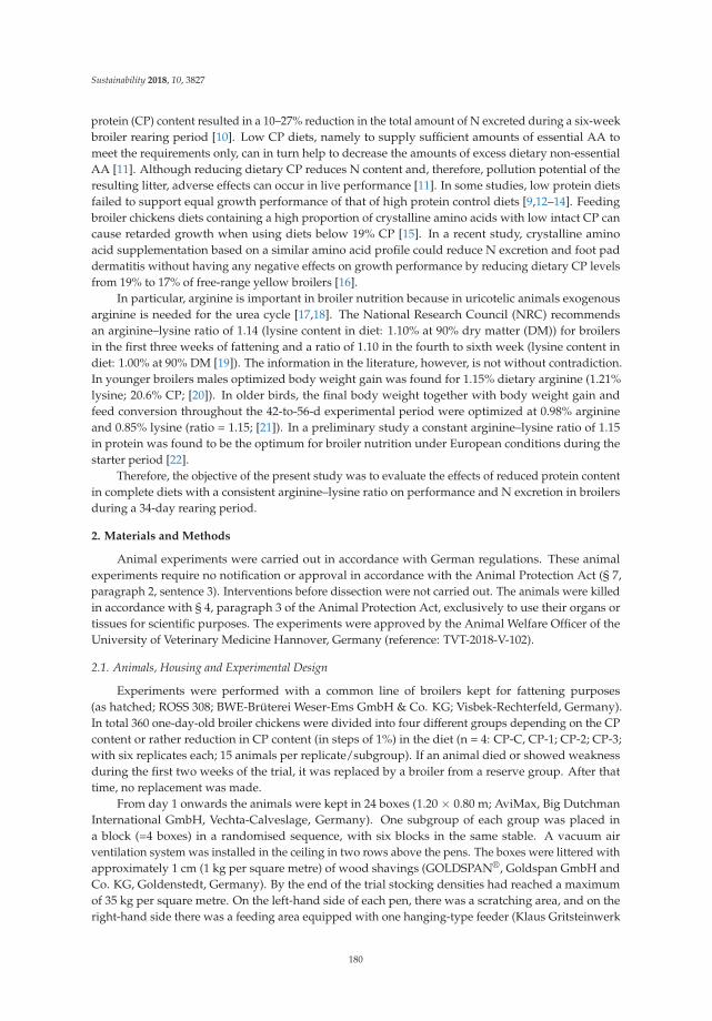
Sustainability 2018, 10, 3827
protein (CP) content resulted in a 10–27% reduction in the total amount of N excreted during a six-weekbroiler rearing period [10]. Low CP diets, namely to supply sufficient amounts of essential AA tomeet the requirements only, can in turn help to decrease the amounts of excess dietary non-essentialAA [11]. Although reducing dietary CP reduces N content and, therefore, pollution potential of theresulting litter, adverse effects can occur in live performance [11]. In some studies, low protein dietsfailed to support equal growth performance of that of high protein control diets [9,12–14]. Feedingbroiler chickens diets containing a high proportion of crystalline amino acids with low intact CP cancause retarded growth when using diets below 19% CP [15]. In a recent study, crystalline aminoacid supplementation based on a similar amino acid profile could reduce N excretion and foot paddermatitis without having any negative effects on growth performance by reducing dietary CP levelsfrom 19% to 17% of free-range yellow broilers [16].
In particular, arginine is important in broiler nutrition because in uricotelic animals exogenousarginine is needed for the urea cycle [17,18]. The National Research Council (NRC) recommendsan arginine–lysine ratio of 1.14 (lysine content in diet: 1.10% at 90% dry matter (DM)) for broilersin the first three weeks of fattening and a ratio of 1.10 in the fourth to sixth week (lysine content indiet: 1.00% at 90% DM [19]). The information in the literature, however, is not without contradiction.In younger broilers males optimized body weight gain was found for 1.15% dietary arginine (1.21%lysine; 20.6% CP; [20]). In older birds, the final body weight together with body weight gain andfeed conversion throughout the 42-to-56-d experimental period were optimized at 0.98% arginineand 0.85% lysine (ratio = 1.15; [21]). In a preliminary study a constant arginine–lysine ratio of 1.15in protein was found to be the optimum for broiler nutrition under European conditions during thestarter period [22].
Therefore, the objective of the present study was to evaluate the effects of reduced protein contentin complete diets with a consistent arginine–lysine ratio on performance and N excretion in broilersduring a 34-day rearing period.
2. Materials and Methods
Animal experiments were carried out in accordance with German regulations. These animalexperiments require no notification or approval in accordance with the Animal Protection Act (§ 7,paragraph 2, sentence 3). Interventions before dissection were not carried out. The animals were killedin accordance with § 4, paragraph 3 of the Animal Protection Act, exclusively to use their organs ortissues for scientific purposes. The experiments were approved by the Animal Welfare Officer of theUniversity of Veterinary Medicine Hannover, Germany (reference: TVT-2018-V-102).
2.1. Animals, Housing and Experimental Design
Experiments were performed with a common line of broilers kept for fattening purposes(as hatched; ROSS 308; BWE-Brüterei Weser-Ems GmbH & Co. KG; Visbek-Rechterfeld, Germany).In total 360 one-day-old broiler chickens were divided into four different groups depending on the CPcontent or rather reduction in CP content (in steps of 1%) in the diet (n = 4: CP-C, CP-1; CP-2; CP-3;with six replicates each; 15 animals per replicate/subgroup). If an animal died or showed weaknessduring the first two weeks of the trial, it was replaced by a broiler from a reserve group. After thattime, no replacement was made.
From day 1 onwards the animals were kept in 24 boxes (1.20 × 0.80 m; AviMax, Big DutchmanInternational GmbH, Vechta-Calveslage, Germany). One subgroup of each group was placed ina block (=4 boxes) in a randomised sequence, with six blocks in the same stable. A vacuum airventilation system was installed in the ceiling in two rows above the pens. The boxes were littered withapproximately 1 cm (1 kg per square metre) of wood shavings (GOLDSPAN®, Goldspan GmbH andCo. KG, Goldenstedt, Germany). By the end of the trial stocking densities had reached a maximumof 35 kg per square metre. On the left-hand side of each pen, there was a scratching area, and on theright-hand side there was a feeding area equipped with one hanging-type feeder (Klaus Gritsteinwerk
180

Sustainability 2018, 10, 3827
GmbH & Co. KG, Bünde, Germany). Drinking lines with nipple drinkers (two nipples per box)for broilers (Big Dutchman International GmbH, Vechta, Germany) were used. The environmentaltemperature was gradually reduced from about 33 ◦C for the one-day-old birds to about 20 ◦C byday 34. Lights were continuously on at days one, two, and three, and the photoperiod from day fouronwards amounted to 16 h of light and 8 h of darkness with dimmed night lighting.
2.2. Diets and Feeding Concept
All birds were fed ad libitum with specifically prepared pelleted diets. For the trial, 12 differentdiets (four different starter diets, four grower diets, and four finisher diets) were produced at theInstitute for Animal Nutrition, University of Veterinary Medicine Hannover, Foundation, Hannover,Germany. One component (80% of diet; Best 3 Geflügelernährung GmbH, Twistringen, Germany)of each of the 12 diets was the same supplementary feed with vitamins, minerals and coccidiostats(narasin/nicarbacin). This maximized the comparability of the final diets with each other.
The remaining 20% of the specific compound feedingstuffs consisted of corn, soybean meal,amino acids and some minerals (limestone, monocalciumphosphate, salt, sodium bicarbonate) to makeup the 12 different experimental diets (Table 1).
Table 1. Ingredient composition of the diets during the whole experimental period. CP: crude protein.
Parameter [%]Starter Grower Finisher
CP-C CP-1 CP-2 CP-3 CP-C CP-1 CP-2 CP-3 CP-C CP-1 CP-2 CP-3
Supplementary Feedingstuff * 80.0 80.0 80.0 80.0 80.0 80.0 80.0 80.0 80.0 80.0 80.0 80.0Corn 0.30 4.51 8.83 13.6 4.31 9.44 13.1 9.95 7.15 10.8 15.3 7.77
Soybean meal 14.8 10.8 6.83 2.40 10.8 6.00 2.40 0.00 8.50 5.25 1.00 0.00Plant oil 3.40 2.68 1.85 1.00 4.15 3.30 2.60 4.35 4.10 3.30 2.50 5.60
Limestone 0.75 0.74 0.73 0.72 0.30 0.29 0.30 0.28 0.05 0.04 0.02 0.00Mono-Ca-phosphate 0.50 0.57 0.63 0.70 0.25 0.33 0.39 0.52 0.00 0.06 0.13 0.26
Salt 0.12 0.08 0.04 0.00 0.10 0.05 0.02 0.00 0.07 0.04 0.00 0.00Sodium Bicarbonate 0.00 0.00 0.05 0.00 0.00 0.06 0.11 0.14 0.00 0.05 0.09 0.10
Arginine 0.00 0.12 0.23 0.36 0.00 0.14 0.25 0.35 0.00 0.10 0.22 0.29Isoleucine 0.00 0.07 0.14 0.21 0.00 0.08 0.15 0.21 0.00 0.06 0.13 0.17
L-Lysine-HCl 0.04 0.17 0.30 0.44 0.04 0.20 0.32 0.42 0.04 0.15 0.29 0.35L-Methionine 0.03 0.05 0.06 0.08 0.00 0.02 0.04 0.06 0.00 0.01 0.03 0.05
Threonine 0.07 0.13 0.19 0.26 0.05 0.01 0.18 0.24 0.08 0.13 0.19 0.24Valine 0.00 0.07 0.13 0.20 0.00 0.08 0.14 0.20 0.00 0.05 0.12 0.17Caolin 0.00 0.00 0.00 0.00 0.00 0.00 0.00 3.32 0.00 0.00 0.00 5.00
* Containing 51.4% wheat, 24.1% soybean meal, 15.0% corn, 5.08% plant oil, 1.30% limestone, 0.94%mono-Ca-phosphate, 0.70% formic acid, 0.40% Alimet, 0.25% enzyme mixture (phytase, xylanase), 0.25% premix,0.22% sodium bicarbonate, 0.22% salt, 0.10% lysine, 0.06% betaine (33%); feed additives per kg: 12,500 IU vitaminA, 6250 IU vitamin D3, 43 mg Vitamin E, 18.7 mg Cu, 25 mg Fe, 87.5 mg Mn, 62.5 mg Zn, 2.5 mg I, 0.37 mg Se,acetic acid, formic acid, 625 FTU 6-phytase, 3000 U Endo 1,4-ß-xylanase, 62.5 mg narasin, 62.5 mg nicarbacin.
One group received a standard control diet (starter: d 1–7, grower: d 8–14; finisher: d 15–35),the other groups, specially prepared experimental diets. The control diet was a complete feedingstuffwith a common protein content (as fed; starter: 21.5% CP; grower: 20.5% CP; finisher: 20.0%CP; each designed for an arginine–lysine ratio of 115:100; Table 2). In the experimental diets,the arginine–lysine ratio was constant; the protein was lower in steps of 1.00 per cent. The levels ofessential amino acids were held at the same level due to the supplementation of single amino acids.To ensure the optimum composition and to verify the ratio between the components, these 12 differentdiets (in total: four starters, growers and finishers each) were analyzed (Table 2).
181
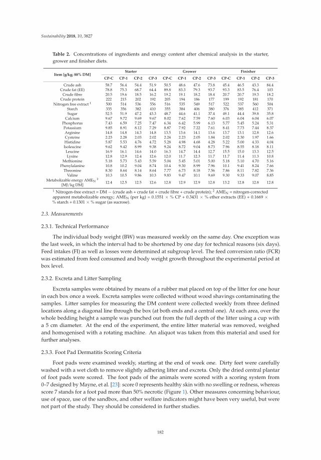
Sustainability 2018, 10, 3827
Table 2. Concentrations of ingredients and energy content after chemical analysis in the starter,grower and finisher diets.
Item [g/kg; 88% DM]Starter Grower Finisher
CP-C CP-1 CP-2 CP-3 CP-C CP-1 CP-2 CP-3 CP-C CP-1 CP-2 CP-3
Crude ash 58.7 56.4 54.4 51.9 50.5 48.6 47.6 73.8 45.4 46.5 43.3 84.4Crude fat (EE) 78.8 75.3 68.7 64.4 89.8 83.3 79.3 93.7 93.3 83.5 76.4 103
Crude fibre 20.5 19.6 18.5 16.2 19.2 19.1 18.2 18.4 20.7 20.7 19.3 18.2Crude protein 222 215 202 192 205 194 186 177 199 192 181 170
Nitrogen free extract 1 500 514 536 556 516 535 549 517 522 537 560 504Starch 335 356 382 410 355 384 406 380 376 385 412 371Sugar 52.5 51.9 47.2 43.3 48.7 44.6 41.1 37.4 49.1 44.4 39.8 35.8
Calcium 9.67 9.72 9.69 9.67 8.02 7.62 7.59 7.60 6.03 6.04 6.04 6.07Phosphorus 7.43 6.59 7.25 7.47 6.34 6.42 5.99 6.13 5.77 5.45 5.24 5.31Potassium 9.85 8.91 8.12 7.29 8.87 7.92 7.22 7.61 8.41 7.73 7.44 8.37Arginine 14.8 14.8 14.3 14.8 13.5 13.6 14.1 13.6 13.7 13.1 12.8 12.6Cysteine 2.23 2.28 2.03 2.02 2.24 2.23 2.05 1.84 2.02 2.30 1.97 1.66Histidine 5.87 5.53 4.76 4.72 5.28 4.98 4.68 4.28 5.22 5.00 4.33 4.04Isoleucine 9.62 9.42 8.99 9.38 9.24 8.72 9.04 8.73 7.96 8.55 8.18 8.11Leucine 16.9 16.1 14.6 14.0 16.3 14.7 14.4 12.7 15.5 15.0 13.3 12.5Lysine 12.8 12.9 12.4 12.6 12.0 11.7 12.3 11.7 11.7 11.4 11.3 10.8
Methionine 5.18 5.73 5.43 5.59 5.04 5.45 5.01 5.00 5.18 5.10 4.70 5.16Phenylalanine 10.8 10.2 9.04 8.74 10.4 9.30 8.99 7.96 10.1 9.41 8.24 7.66
Threonine 8.30 8.64 8.14 8.64 7.77 6.73 8.18 7.56 7.86 8.11 7.82 7.36Valine 10.3 10.5 9.86 10.3 9.83 9.47 10.1 9.69 9.30 9.33 9.07 8.85
Metabolizable energy AMEN2
[MJ/kg DM]12.4 12.5 12.5 12.6 12.8 12.9 12.9 12.8 13.2 12.8 12.8 12.8
1 Nitrogen-free extract = DM − (crude ash + crude fat + crude fibre + crude protein); 2 AMEN = nitrogen-correctedapparent metabolizable energy; AMEN (per kg) = 0.1551 × % CP + 0.3431 × % ether extracts (EE) + 0.1669 ×% starch + 0.1301 × % sugar (as sucrose).
2.3. Measurements
2.3.1. Technical Performance
The individual body weight (BW) was measured weekly on the same day. One exception wasthe last week, in which the interval had to be shortened by one day for technical reasons (six days).Feed intakes (FI) as well as losses were determined at subgroup level. The feed conversion ratio (FCR)was estimated from feed consumed and body weight growth throughout the experimental period atbox level.
2.3.2. Excreta and Litter Sampling
Excreta samples were obtained by means of a rubber mat placed on top of the litter for one hourin each box once a week. Excreta samples were collected without wood shavings contaminating thesamples. Litter samples for measuring the DM content were collected weekly from three definedlocations along a diagonal line through the box (at both ends and a central one). At each area, over thewhole bedding height a sample was punched out from the full depth of the litter using a cup witha 5 cm diameter. At the end of the experiment, the entire litter material was removed, weighedand homogenised with a rotating machine. An aliquot was taken from this material and used forfurther analyses.
2.3.3. Foot Pad Dermatitis Scoring Criteria
Foot pads were examined weekly, starting at the end of week one. Dirty feet were carefullywashed with a wet cloth to remove slightly adhering litter and excreta. Only the dried central plantarof foot pads were scored. The foot pads of the animals were scored with a scoring system from0–7 designed by Mayne, et al. [23]: score 0 represents healthy skin with no swelling or redness, whereasscore 7 stands for a foot pad more than 50% necrotic (Figure 1). Other measures concerning behaviour,use of space, use of the sandbox, and other welfare indicators might have been very useful, but werenot part of the study. They should be considered in further studies.
182

Sustainability 2018, 10, 3827
Figure 1. Foot pad lesions with different scores. (a) Score 0: no alterations detected; and (b) Score7: more than half of the foot pad covered with necrotic cells (photo: ©University of VeterinaryMedicine, Hannover).
2.3.4. Dissection
After 35 days, 120 animals (n = 30 per group) were dissected. A percussive blow to the head wasused as anaesthesia or rather the stunning method in accordance with Annex I of Council Regulation(EC) No. 1099/2009, Chapter I, Methods, Table 1—Mechanical methods, No. 6. After bleeding theanimals, the body cavity was opened, the sternum lifted up and samples of the ileum were taken forhistological investigations. All remaining birds were sold.
2.3.5. Histological Investigations
For histological investigations, an approximately 1 cm long piece was removed from the ileum(in the middle between the diverticulum and cranial part of the caecum) and fixed in 4% formaldehydefor 48 h. After fixation, tissue samples were embedded in paraffin using standard techniques [24].For histological evaluation, 4 μm sections of all samples were stained with haematoxylin and eosin(HE) using established protocols [24]. The villus height was measured from the tip of the villi to thevillus crypt junction; villus width was measured at the base of the villus above the villus crypt junctionusing a Zeiss axioscope (Carl Zeiss Jena GmbH, Jena, Germany).
2.3.6. Analysis of Feed, Excreta, and Litter Samples
The official methods of the VDLUFA were the basis of the standard procedures being used toanalyze all diets [25]. Determining the dry matter content and the crude ash content works throughaction of heat; drying the samples to the weight constancy at 103 ◦C delivers the results for the DMcontent. Through combustion of the sample at 600 ◦C in a muffle furnace the crude ash contentwas analyzed. The total N content was determined by the DUMAS combustion method (Vario Max,Elementar, Hanau, Germany). The crude fat content was determined by standard protocol (soxhletapparatus). Crude fiber was analyzed after washing in dilute acids and alkalis. Starch determinationwas carried out polarimetrically (Polatronic E, Schmidt und Haensch GmbH & Co., Berlin, Germany).The Luff-Schoorl method was used to determine the sugar content. Minerals were analyzed byatomic absorption spectrometry (Unicam Solaar 116, Thermo, Dreieich, Germany). Amino acids weredetermined by ion-exchange chromatography (AA analyzer LC 3000, Biotronic, Maintal, Germany).
2.3.7. Estimations of Efficiencies of Nitrogen or Rather Protein Utilisation
The single box was the observation unit for assessing nutrient efficiency between groups. The basisfor the considerations was the total FI in the box, the increase in body weight (final body weight minus
183

Sustainability 2018, 10, 3827
weight at hatch; including the increase in deceased animals), and the amount of final litter materialin the box. The N content in the different diets and in the litter were analyzed by standard methodsdescribed above (2.2.6). To calculate the N content in the fresh whole body of birds (including feathers),crude protein contents from various publications were used as a basis [12,26–28]. From the means(in g N/100 g fresh total body: 3.312 [27], 3.016 [26], 2.754 [28], 2.598 [12]) a factor was derived(2.920) and used as the basis for calculating parameters in accordance with Aletor, Hamid, Niess andPfeffer [26], modified.
N-retention efficiency (%) = g N retained/g N consumed × 100
N-efficiency rate = g weight gain/g N consumed
N excretion (apparent) = g N consumed − g N retained
2.4. Statistical Analysis
Data analyses were performed using the SAS statistical software package version 7.1 (SAS Inst.,Cary, NC, USA). Mean values, as well as the standard deviation of the mean (standard deviation (SD)),were calculated for all parameters. The mean footpad dermatitis (FPD) scores were evaluated by usingthe mean of both feet. For the values of body weight (BW), the foot pad dermatitis scores and theresults of the histopathological investigations as well as the individuum were the basis of observation.All other parameters were analyzed at box-level. The group comparisons were performed by one-wayanalysis of variance (ANOVA) for independent samples. In general, the Ryan–Einot–Gabriel–Welschmultiple-range test (REGWQ) was used for multiple pairwise means comparisons between the fourgroups. All statements of statistical significance were based on p < 0.05.
3. Results
The experiments ran without complications. From the start of week 3, six out of 360 animals died(CP-C: 2; CP-1: 1; CP-2: 1; CP-3:2). There was no antibiotic treatment during the trial.
3.1. Technical Performance
Results relating to growth performance of broilers are shown in Table 3. At day 1, the averageweight per chicken was 43.0 g. In broilers, after 34 days of fattening, BW exceeded the performancegoals of the breeding company [29]. At the end of the first and the second week of fattening the BWalready showed significant differences between groups, being lowest in group CP-3 (Table 3). In weeksthree, four, and five, birds in group CP-2 were significantly heavier than in groups CP-C and CP-3.
Table 3. Average body weight and feed conversion ratio (FCR) during the trial (mean ± standarddeviation (SD)).
Item Group Week 1 Week 2 Week 3 Week 4 Week 5 *
Body weight[in g; end of week]
CP-C 216 A ± 19.8 535 A ± 58.1 989 B,C ± 116 1589 B,C ± 189 2192 B,C ± 258CP-1 218 A ± 16.5 541 A ± 51.7 1004 A,B ± 116 1632 A,B ± 199 2244 A,B ± 275CP-2 217 A ± 15.6 552 A ± 47.1 1034 A ± 106 1678 A ± 182 2329 A ± 266CP-3 206 B ± 20.1 517 B ± 45.6 956 C ± 99.8 1548 C ± 175 2131 C ± 244
FCR [Ø in week]
CP-C 0.987 ± 0.073 1.169 ± 0.023 1.363 ± 0.043 1.488 ± 0.039 1.848 ± 0.066CP-1 0.952 ± 0.034 1.185 ± 0.025 1.342 ± 0.026 1.474 ± 0.026 1.817 ± 0.020CP-2 0.996 ± 0.044 1.165 ± 0.009 1.334 ± 0.047 1.494 ± 0.032 1.776 ± 0.050CP-3 1.025 ± 0.070 1.199 ± 0.042 1.389 ± 0.047 1.518 ± 0.026 1.827 ± 0.104
A,B,C averages differ significantly within a column (p < 0.05); * only six days—measurement end of day 34.
No differences were observed concerning the feed conversion rate (FCR) in broilers dependingon the dietary feeding concept. The FCR showed numerically lowest values for group CP-2 duringthe entire period (CP-C: 1.474 ± 0.036; CP-1: 1.457 ± 0.010; CP-2: 1.454 ± 0.017; CP-3: 1.489 ± 0.016,respectively).
184

Sustainability 2018, 10, 3827
3.2. Excreta and Litter Quality
There were no differences in DM content of excreta between groups CP-C, CP-1 and CP-2 (Table 4).Excreta of group CP-3 were the driest from week two onwards. The control group had the wettestlitter in the fourth week of fattening. At the end of the experiment, groups CP-C, CP-1 and CP-2 werenot significantly different concerning DM content in litter. The group CP-3 had the driest litter at weekfive. The litter material was finally removed from the boxes. The dry matter content was significantlyhigher in material from group CP-3 than in the other groups (in g DM/kg; CP-C: 584 B ± 31.3; CP-1:602 B ± 39.7; CP-2: 603 B ± 44.4; CP-3: 698 A ± 30.7, respectively).
Table 4. Dry matter content of excreta and litter material during the five-week trial period (mean ± SD).
Item Group Week 1 Week 2 Week 3 Week 4 Week 5 *
Dry matter (DM)excreta †
[in g/kg; end of week]
CP-C 188 B ± 8.34 200 B ± 10.8 189 B ± 7.92 188 B ± 9,31 184 B ± 9.46CP-1 193 A,B ± 9.27 208 B ± 9.27 188 B ± 6.62 186 B ± 11.9 184 B ± 8.18CP-2 199 A,B ± 14.8 207 B ± 12.1 192 B ± 16.9 184 B ± 14.2 181 B ± 8.01CP-3 206 A ± 9.47 228 A ± 7.25 228 A ± 20.2 232 A ± 2.76 219 A ± 9.77
Dry matter litter ‡
[in g/kg; end of week]
CP-C 815 ± 36.2 816 B ± 23.9 712 A,B ± 53.8 588 B ± 54.3 609 B ± 69.8CP-1 829 ± 29.3 837 A,B ± 24.6 698 B ± 42.2 596 A,B ± 67.6 610 B ± 31.3CP-2 817 ± 31.5 831 A,B ± 43.9 718 A,B ± 58.0 617 A,B ± 58.0 584 B ± 61.6CP-3 830 ± 30.7 856 A ± 24.3 763 A ± 49.7 667 A ± 66.7 709 A ± 45.1
A,B averages differ significantly within a column (p < 0.05); * only six days—measurement end of day 34;† REGWQ-test; ‡ LSD-test.
Analyzing the N content in the excreta showed that diets with lower CP content led to significantlylower N values in the excreta (Table 5). In comparison to the control, in week 5 the N content wasreduced by 36.6%. Also, the mean N content in the total litter was significantly lower in group CP-3(36.2 ± 1.64 g/kg DM) than in all other groups. Additionally, group CP-2 (46.2 ± 1.30 g/kg DM)showed significantly lower concentrations of N in the total litter compared to the material from thegroups CP-1 (49.7 ± 1.57 g/kg DM) and CP-C (51.2 ± 2.22 g/kg DM).
Table 5. Nitrogen content in excreta during the five-week trial period (mean ± SD).
Item Group Week 1 Week 2 Week 3 Week 4 Week 5
Nitrogen content[in g/kg DM; end of week]
CP-C 44.7 A ± 2.16 43.5 A ± 1.45 44.8 A ± 1.28 46.3 A ± 1.43 50.0 A ± 3.13CP-1 43.4 A,B ± 2.05 38.7 B ± 0.71 42.1 B ± 1.79 45.0 A ± 1.59 47.9 A ± 3.02CP-2 40.4 A,B ± 2.12 36.4 C ± 2.01 36.4 C ± 2.56 41.2 B ± 1.94 42.4 B ± 2.64CP-3 35.4 C ± 3.03 29.1 D ± 0.86 28.4 D ± 1.29 29.7 C ± 1.63 31.7 C ± 1.99
A,B,C averages differ significantly within a column (p < 0.05).
The level of FI and the protein content in the feed determined the average total N intake perbox. The birds in group CP-2 showed the significantly highest FI compared to groups CP-1 and CP-3(per animal; CP-C: 3169 B g, CP-1: 3210 A,B g; CP-2: 3323 A g; CP-3 3107 C g, respectively). Total Nuptake was significantly higher in the control group than in CP-2 and CP-3 (Table 6). The total amountof N in the litter material harvested at the end of the experiment was gradually reduced analogous tothe protein reduction in the feed. The group CP-2 showed the highest absolute weight gain per boxand accordingly the highest absolute N retention per box compared to the other groups.
Table 6. Estimations of nitrogen balance over the entire trial period (mean ± SD).
GroupN-Intake From
Feed [g/box]N-Amount in
Final Litter [g/box]Weight Gain Δ
Final-Start [g/box]N-Retained
[g/box]
CP-C 1517 A ± 52.5 581 A ± 39.6 32,033 B,C ± 781 938 B ± 22.8CP-1 1484 A,B ± 52.9 522 B ± 28.2 32,923 A,B ± 1147 938 B ± 22.9CP-2 1451 B ± 35.8 477 C ± 25.3 34,190 A ± 987 1001 A ± 28.8CP-3 1278 C ± 30.8 416 D ± 20.0 31,220 C ± 803 914 B ± 23.5
A,B,C,D averages differ significantly within a column (p < 0.05).
185

Sustainability 2018, 10, 3827
The N retention efficiency in the groups CP-C and CP-1 was significantly worse than in the groupsCP-2 and CP-3 (Table 7). Compared to the control, the efficiency could be improved step by step by 1.4,7.1 and 9.6 percentage points from CP-1 to CP-3, respectively.
Table 7. Estimations of efficiencies of nitrogen utilization (mean ± SD).
GroupN-Retention
Efficiency * [%]N-EfficiencyRatio † [g/g]
N-Excretion (Apparent) ‡
[g/box]N-Excretion (Apparent) ‡
[g/animal]
CP-C 61.9 C ± 1.46 21.1 D ± 0.50 579 A ± 39.8 38.6 A ± 2.66CP-1 63.3 C ± 2.76 22.2 C ± 0.17 546 A ± 56.7 36.4 A ± 3.78CP-2 69.0 B ± 0.81 23.6 B ± 0.28 450 B ± 15.2 30.0 B ± 1.01CP-3 71.5 A ± 0.70 24.4 A ± 0.24 364 C ± 12.6 24.2 C ± 0.84
A,B,C,D averages differ significantly within a column (p < 0.05). * Nitrogen retention efficiency (%) = (g N retained/gN consumed) × 100; † Nitrogen efficiency rate = g weight gain/g N consumed; ‡ Nitrogen excretion (apparent) = gN consumed − g N retained.
3.3. Footpad Dermatitis
In this trial there were no clinical issues concerning foot pad health. The foot pad health was verygood overall (Table 8). A comparison between groups showed significant differences at the end of thethird week. In group CP-2, the scores were significantly higher.
Table 8. Foot pad (FPD) scores in broilers during the five-week trial period (mean ± SD).
Item Group Week 1 Week 2 Week 3 Week 4 Week 5
FPD Scores[averages of both feet; end of week]
CP-C 0.04 ± 0.13 0.46 ± 0.38 0.94 B ± 0.20 0.97 ± 0.15 0.68 ± 0.39CP-1 0.03 ± 0.12 0.43 ± 0.37 1.02 A,B ± 0.23 0.97 ± 0.12 0.61 ± 0.41CP-2 0.05 ± 0.17 0.38 ± 0.37 1.04 A ± 0.23 0.97 ± 0.12 0.63 ± 0.40CP-3 0.03 ± 0.12 0.45 ± 0.38 0.99 A,B ± 0.28 1.01 ± 0.12 0.74 ± 0.41
A,B averages differ significantly within a column (p < 0.05).
3.4. Histological Investigations
There were no differences in the results of the histological examinations (Table 9).
Table 9. Average villus height * and villus width in the ileum of broilers (mean ± SD).
Item Group Dissection
Villus height * [in μm]
CP-C 454 ± 68.3CP-1 448 ± 58.1CP-2 455 ± 50.4CP-3 446 ± 75.9
Villus width † [in μm]
CP-C 139 ± 23.0CP-1 142 ± 18.1CP-2 140 ± 26.9CP-3 140 ± 25.8
* Villus height was measured from the tip of the villi to the villus crypt junction; † villus width was measured at thebase of the villus above the villus crypt junction.
The intestinal wall of the ileum showed no alterations (Figure 2).
186

Sustainability 2018, 10, 3827
Figure 2. HE staining from ileal intestinal wall of broiler chickens with CP-1 diet. Scale bars = 500 μm.
4. Discussion
The investigations were conducted without incidents. Animal losses were very low (1.66%mortality) from day 14 onwards. Performance parameters were above performance goals of thebreeding company [29]. With a final average body weight between 2131 g (CP-3) and 2329 g (CP-2),the body weight development excelled the guidelines of the breeding organization (2050 g). Thus,the performance was higher in each group (CP-C: +6.93%; CP-1: +9.46%; CP-2: +13.6%; CP-3: +3.95%,respectively). Moreover, the feed utilization per kg body weight gain was lower in all groups comparedto the performance goals (cumulative feed expenditure in accordance with Aviagen [29]: 1528;reduction: CP-C: −3.53%; CP-1: −4.65%; CP-2: −4.84%; CP-3: −2.55%, respectively). Moran et al. [11]observed in early studies on CP reduction (downwards to 17.8%; weeks 4–6) an increase in feed to gainratio from 1.72 to 1.76. However, the rations were balanced only with L-lysine HCl, DL-methionine,and L-threonine. The arginine–lysine ratio was therefore not optimal, this being 1.04 in the first threeweeks (20.8% CP) and 0.99 in weeks 4–6 (17.8% CP). In a frequently cited study by Bregendahl et al. [12],the performance deteriorated when reducing the protein content to a level comparable to ours inthe present study. In the study mentioned above [12], at protein levels of 185–186.5 g CP per kgdiet and supplementation of identical amino acids used in our study, complemented by glutamine,the performance was lower compared to the control (23% CP). Nonetheless, the two investigationsdiffer in terms of the absolute levels of supplemented amino acids. Especially methionine seemedto be much higher in the study of Bregendahl et al. [12]. Namroud et al. [15] were able to show acomparable body weight in broilers using crystalline amino acids in protein reduced diets (reduction of23% to 19% CP at day 28). A further reduction to 17% CP led to a significant decrease in the final bodyweight at day 28 by 17.5%. In comparison to Namroud et al. [15], no comparable effect occurred inthe present study, although reduction in CP content was nearly the same (a decrease to 17.7% percentby day 14 or to 17% thereafter). The greatest difference between Namroud et al. [15] and the presenttrial can be seen in the methionine content (approx. 1 g higher for Namroud et al. [15]), and leucine(up to 5 g surplus in the study of Namroud et al. [15]). In studies with free-range chickens, however,observations were in line with the present study [16]. The performance was comparable when reducing
187

Sustainability 2018, 10, 3827
from 19% to 17% CP and balancing essential amino acid content. From these observations, it can beconcluded that with increasing crude protein reduction, the targeted application of certain aminoacids must be given more emphasis if performance is to be maintained. Feed costs represent about70% of the cost of poultry production [30]. Therefore, this makes a bird’s ability to use feed efficientlyvery important [30]. Precisely following the nutritional requirements of poultry is the guarantor foroptimum feed efficiency [30]. Therefore, studies like this can help to maintain profitability while at thesame time taking into account other aspects of sustainability like ecological dimensions of production.
In the present investigations, the N content in the excreta could be lowered significantly using CPreduced diets. The N content in the excreta was reduced by up to 36.6% at a comparable performanceby reducing the protein content from 20% to 17% (reduction in N content in excreta compared toCP-C in week 5: CP-1: −4.20%; CP-2: −15.2%; CP-3: −36.6%, respectively). The ratios were alsoreflected in the content of the entire litter material. The protein reduction of up to 3% starting froma diet with moderate protein content in the present study resulted in a reduction in the N contentin the total litter material of up to 37.3% (N reduction in litter compared to CP-C: CP-1: −5.70%;CP-2: −22.3%; CP-3: −37.3%, respectively). The N efficiency could be further increased by almost 10percentage points (CP-C: 61.9%; CP-3: 71.5%, respectively) due to the feeding concept, in spite of analready high efficiency. The present investigations are in line with the results of Ospina-Rojas et al. [9].This research group was able to reduce the N content in the litter from 47.2 g N/kg DM to 31.9 g N/kgDM (−32.4%) by reducing the protein content in the diet from 19% to 16% by supplementing valine,isoleucine, arginine and glycine achieving a constant performance. When supplementation of valine,isoleucine and glycine or valine, isoleucine and arginine or of all four aforementioned amino acidswas not made, a significant performance depression occurred [9]. Blair et al. [10] were able to achievea reduction in the N content in the excreta from 52.5 g/kg DM to 47.2 g/kg DM without affectingthe performance by reducing the protein contents from 21% to 18% in weeks 3 to 6 while balancingessential amino acids. The N retention could be increased from 47% to 51%. In the same study, the Nretention could be increased from 61% to 63% under conditions of a total of 6 weeks’ adjustment inthe protein content. Namroud et al. [15] were able to reduce the N content in excreta from 50.3 g/kgDM to 36.3 g/kg DM (−27.8%) by achieving a constant amino acid content in the diet, reducing thecrude protein content from 23% to 17%. Shao et al. [16] were able to reduce the N content in theexcreta from 65.2 g/kg DM to 47.3 g/kg DM (−27.4%) in free-range chickens by reducing the proteincontent from 19% to 17%. In the present investigations, the reduction in the N content in excreta orlitter material was higher in its peak than in the aforementioned publications. Overall, the proteinreduction was accompanied to a certain extent by an increased performance (CP-2), which was alsoreflected in the high absolute N efficiency. The current global production of ammonia, CH4, and N2Oby the poultry industry is significant [30]. Improvements in feed conversion ratio have a favorableeffect on environmental emissions and decrease the environmental impact of poultry production [30].Therefore, the present investigations thus show that the environment can be relieved to the maximumby continuously optimizing the rations.
In this study, no clinical problems concerning the foot pad health of the broilers could bedetermined, independent of CP level in the diets. After 34 days of fattening, nearly 100% of thebroilers had an FPD score ≤1, despite the high stocking density of about 35 kg/m2. Only one animalin group CP-C and three animals in group CP-3 had a score of 2 in one foot. Therefore, the results ofthis study show neither negative nor positive effects of using the different dietary concepts.
The results of the histological examination were used to check whether the reduction in the proteincontent also had an influence on intestinal histology. The results of the study gave no indication of this.
With maximum protein reduction (CP-3), we used a diet containing kaolin at the beginningof the third fattening week effectuating a dilution of the ration. Due to the kaolin the effect ofdifferences in diet composition between the feeding phases and between the groups in one feedingphase (80% supplement concept) was minimized. However, it cannot be ruled out that this ingredientmight have influenced the FI. The results of the investigations suggest that further analyses would
188

Sustainability 2018, 10, 3827
be useful. In these investigations the use of kaolin should be avoided on the one hand. Furthermore,it should be examined to what extent very expensive amino acids such as isoleucine etc. have tobe completely balanced in the rations. If reductions are possible, this would allow the alreadyeconomical concept to be continuing optimized and at the same time the environmental burden couldbe further reduced.
5. Conclusions
The potential environmental impact is an important evaluation factor for the sustainability ofanimal production. Meticulous balanced protein-reduced diets allow a significant reduction in theuse of nutrients, especially in high N containing components. Under these conditions, the adjustmentof the amino acid content becomes more and more important if the performance is at least keptconstant. As the degree of crude protein reduction increases, N excretion falls disproportionately.This nutritional intervention enables significant improvements in terms of the environmental impactof animal production.
Author Contributions: Conceptualization, C.V., V.T. and D.S.; Methodology, C.V., M.L. and R.B.; Validation, C.V.,C.U., M.L. and R.B.; Formal Analysis, C.U. and C.V.; Investigation, C.U., M.L. and C.V.; Resources, C.V., V.T. andR.B.; Data Curation, C.U. and C.V.; Writing—Original Draft Preparation, C.U. and C.V.; Writing—Review &Editing, C.U., M.L., R.B., V.T., D.S. and C.V.; Visualization, C.U., C.V., M.L. and R.B.; Supervision, C.V. and R.B.;Project Administration, C.V. and R.B.; Funding Acquisition, C.V.
Funding: The study was financially supported by CJ Europe GmbH, Schwalbach, Germany. The role of thefunding body was merely financial. The CJ Europe GmbH did not have any role in collecting, interpreting,analyzing or writing up the data. This publication was also supported by the Deutsche Forschungsgemeinschaftand University of Veterinary Medicine Hannover, Foundation, Germany within the funding program OpenAccess Publishing.
Acknowledgments: We would like to thank Frances Sherwood-Brock for proof-reading the manuscript to ensurecorrect English.
Conflicts of Interest: Venja Taube is an employee of BEST 3 Gefluegelernaehrung GmbH, Twistringen, Germany.The BEST 3 Gefluegelernaehrung GmbH had no role in the design of the study; in the collection, analyses,or interpretation of data; in the writing of the manuscript, or in the decision to publish the results. Diana Siebert isan employee of CJ Europe GmbH, Schwalbach, Germany. The CJ Europe GmbH had no role in the design of thestudy; in the collection, analyses, or interpretation of data; in the writing of the manuscript, or in the decision topublish the results.
References
1. De Vries, M.; de Boer, I.J.M. Comparing environmental impacts for livestock products: A review of life cycleassessments. Livestig. Sci. 2010, 128, 1–11. [CrossRef]
2. Steinfeld, H.; Gerber, P.; Wassenaar, T.; Castel, V.; Rosales, M.; Rosales, M.; de Haan, C. Livestock’s LongShadow: Environmental Issues and Options; Food & Agriculture Org.: Rome, Italy, 2006.
3. Leip, A.; Billen, G.; Garnier, J.; Grizzetti, B.; Lassaletta, L.; Reis, S.; Simpson, D.; Sutton, M.A.; De Vries, W.;Weiss, F. Impacts of european livestock production: Nitrogen, sulphur, phosphorus and greenhouse gasemissions, land-use, water eutrophication and biodiversity. Environ. Res. Lett. 2015, 10, 115004. [CrossRef]
4. Meier, M.S.; Stoessel, F.; Jungbluth, N.; Juraske, R.; Schader, C.; Stolze, M. Environmental impacts oforganic and conventional agricultural products—Are the differences captured by life cycle assessment?J. Environ. Manag. 2015, 149, 193–208. [CrossRef] [PubMed]
5. Ferket, P.R.; van Heugten, E.; van Kempen, T.A.T.G.; Angel, R. Nutritional strategies to reduce environmentalemissions from nonruminants. J. Anim. Sci. 2002, 80, E168–E182. [CrossRef]
6. Mallin, M.A.; Cahoon, L.B. Industrialized animal production—A major source of nutrient and microbialpollution to aquatic ecosystems. Popul. Environ. 2003, 24, 369–385. [CrossRef]
7. Clark, M.; Tilman, D. Comparative analysis of environmental impacts of agricultural production systems,agricultural input efficiency, and food choice. Environ. Res. Lett. 2017, 12, 064016. [CrossRef]
8. Leip, A.; Weiss, F.; Lesschen, J.; Westhoek, H. The nitrogen footprint of food products in the european union.J. Agric. Sci. 2014, 152, 20–33. [CrossRef]
189

Sustainability 2018, 10, 3827
9. Ospina-Rojas, I.C.; Murakami, A.E.; Duarte, C.R.A.; Eyng, C.; Oliveira, C.A.L.; Janeiro, V. Valine, isoleucine,arginine and glycine supplementation of low-protein diets for broiler chickens during the starter and growerphases. Br. Poult. Sci. 2014, 55, 766–773. [CrossRef] [PubMed]
10. Blair, R.; Jacob, J.P.; Ibrahim, S.; Wang, P. A quantitative assessment of reduced protein diets and supplementsto improve nitrogen utilization. J. Appl. Poult. Res. 1999, 8, 25–47. [CrossRef]
11. Moran, E.T.; Bushong, R.D.; Bilgili, S.F. Reducing dietary crude protein for broilers while satisfyingamino-acid-requirements by least-cost formulation—Live performance, litter composition, and yield offast-food carcass cuts at 6 weeks. Poult. Sci. 1992, 71, 1687–1694. [CrossRef]
12. Bregendahl, K.; Sell, J.L.; Zimmerman, D.R. Effect of low-protein diets on growth performance and bodycomposition of broiler chicks. Poult. Sci. 2002, 81, 1156–1167. [CrossRef] [PubMed]
13. Laudadio, V.; Passantino, L.; Perillo, A.; Lopresti, G.; Passantino, A.; Khan, R.; Tufarelli, V. Productiveperformance and histological features of intestinal mucosa of broiler chickens fed different dietary proteinlevels. Poult. Sci. 2012, 91, 265–270. [CrossRef] [PubMed]
14. Laudadio, V.; Dambrosio, A.; Normanno, G.; Khan, R.U.; Naz, S.; Rowghani, E.; Tufarelli, V. Effect of reducingdietary protein level on performance responses and some microbiological aspects of broiler chickens undersummer environmental conditions. Avian Biol. Res. 2012, 5, 88–92. [CrossRef]
15. Namroud, N.F.; Shivazad, M.; Zaghari, M. Effects of fortifying low crude protein diet with crystalline aminoacids on performance, blood ammonia level, and excreta characteristics of broiler chicks. Poult. Sci. 2008, 87,2250–2258. [CrossRef] [PubMed]
16. Shao, D.; Shen, Y.R.; Zhao, X.; Wang, Q.; Hu, Y.; Shi, S.R.; Tong, H.B. Low-protein diets with balanced aminoacids reduce nitrogen excretion and foot pad dermatitis without affecting the growth performance and meatquality of free-range yellow broilers. Ital. J. Anim. Sci. 2018, 17, 698–705. [CrossRef]
17. Khajali, F.; Wideman, R. Dietary arginine: Metabolic, environmental, immunological and physiologicalinterrelationships. World Poult. Sci. J. 2010, 66, 751–766. [CrossRef]
18. Wu, G.; Bazer, F.W.; Dai, Z.; Li, D.; Wang, J.; Wu, Z. Amino acid nutrition in animals: Protein synthesis andbeyond. Annu. Rev. Anim. Biosci. 2014, 2, 387–417. [CrossRef] [PubMed]
19. Council, N.R. Nutrient Requirements of Poultry; National Academic Press: Washington, DC, USA, 1994.20. Corzo, A.; Kidd, M. Arginine needs of the chick and growing broiler. Int. J. Poult. Sci. 2003, 2, 379–382.21. Corzo, A.; Moran, E., Jr.; Hoehler, D. Arginine need of heavy broiler males: Applying the ideal protein
concept. Poult. Sci. 2003, 82, 402–407. [CrossRef] [PubMed]22. Siebert, D.; Khan, D.R.; Esteve-Garcia, E. Investigations on the optimal arginine:lysine ratio in the starter
phase of meat-type chickens. In Proceedings of the 21st European Society of Veterinary and Comparative NutritionCongress; Harris, P., Moore-Colyer, M., Eds.; European Society of Veterinary & Comparative Nutrition:Cirencester, UK, 2017; Volume 21, p. 144.
23. Mayne, R.; Else, R.; Hocking, P. High litter moisture alone is sufficient to cause footpad dermatitis in growingturkeys. Br. Poult. Sci. 2007, 48, 538–545. [CrossRef] [PubMed]
24. Slaoui, M.; Fiette, L. Histopathology procedures: From tissue sampling to histopathological evaluation.In Drug Safety Evaluation; Springer: Cham, Switzerland, 2011; pp. 69–82.
25. Naumann, C.; Bassler, R. Methoden der Landwirtschaftlichen Forschungs-und Untersuchungsanstalt, BiochemischeUntersuchung von Futtermitteln; Methodenbuch iii (einschließlich der achten Ergänzungen); VDLUFA:Darmstadt, Germany, 2012.
26. Aletor, V.A.; Hamid, I.I.; Niess, E.; Pfeffer, E. Low-protein amino acid-supplemented diets in broilerchickens: Effects on performance, carcass characteristics, whole-body composition and efficiencies ofnutrient utilisation. J. Sci. Food. Agric. 2000, 80, 547–554. [CrossRef]
27. Ernährungsphysiologie, G.F. Empfehlungen zur Energie-und Nährstoffversorgung der Legehennen und Masthühner(Broiler); DLG Verlag: Frankfurt am Main, Germany, 1999.
28. Kamran, Z.; Sarwar, M.; Nisa, M.; Nadeem, M.; Ahmad, S.; Mushtaq, T.; Ahmad, T.; Shahzad, M. Effect oflowering dietary protein with constant energy to protein ratio on growth, body composition and nutrientutilization of broiler chicks. Asian Austral J. Anim. 2008, 21, 1629–1634. [CrossRef]
190

Sustainability 2018, 10, 3827
29. Aviagen. Ross 308 Broiler Performance Objectives; Aviagen Group: Huntsville, AL, USA, 2014.30. Willems, O.; Miller, S.; Wood, B. Aspects of selection for feed efficiency in meat producing poultry. World Poult.
Sci. J. 2013, 69, 77–88. [CrossRef]
© 2018 by the authors. Licensee MDPI, Basel, Switzerland. This article is an open accessarticle distributed under the terms and conditions of the Creative Commons Attribution(CC BY) license (http://creativecommons.org/licenses/by/4.0/).
191

sustainability
Article
Production of Pig Feed under Future AtmosphericCO2 Concentrations: Changes in Crop Content andChemical Composition, Land Use, EnvironmentalImpact, and Socio-Economic Consequences
Henrik Saxe 1,* ID , Lorie Hamelin 2, Torben Hinrichsen 3 and Henrik Wenzel 4
1 Mindful Food Solutions, Engbakkevej 3C, 2900 Charlottenlund, Denmark2 Department of Engineering of Biological Systems and Processes (LISBP),
National Institute of Applied Sciences (INSA), INRA UMR792 and CNRS UMR5504,Federal University of Toulouse, 135 Avenue de Rangueil, F-31077 Toulouse, France;[email protected]
3 DSM Nutritional Products Ltd., Kirkebjerg Alle 88, 2605 Brøndby, Denmark; [email protected] Institute of Chemical Engineering, Biotechnology and Environmental Technology,
SDU Life Cycle Engineering, University of Southern Denmark, Campusvej 55, 5230 Odense M, Denmark;[email protected]
* Correspondence: [email protected]; Tel.: +45-60742225
Received: 14 August 2018; Accepted: 2 September 2018; Published: 6 September 2018
Abstract: With the rising atmospheric CO2, crops will assimilate more carbon. Yields will increasein terms of carbohydrates while diluting the content of protein and minerals in compound pigfeed, calling for an altered formulation with more protein and less carbohydrate crops to maintainits nutritional value. Using crop response data from CO2 exposures in a linear modeling of feedformulation, we apply a consequential life cycle assessment (cLCA) to model all of the environmentalimpacts and socio-economic consequences that altered crop yields and chemical composition atelevated CO2 levels have on feed formulation, targeting altered amino acid contents rather thanoverall protein. An atmospheric CO2 of 550 μmole mole−1 gives rise to a 6% smaller demand forland use for pig feed production. However, feed produced at this CO2 must include 23% moresoymeal and 5% less wheat than at present in order to keep its nutritional value. This counteracts theyield benefit. The monetized environmental cost of producing pig feed, where sunflower and soycontribute the most, equals the direct feed price in both scenarios. If external costs were internalized,honoring the Rio Declaration, feed prices would double. In contrast, the future composition of pigfeed will increase the direct price by only 0.8%, while the external cost decreases by only 0.3%.
Keywords: amino acids; compound pig feed formulation; consequential life cycle assessment; cLCA;land-use changes (LUC); monetized environmental impact; protein crops; starch (energy) crops
1. Introduction
During this century, the rising atmospheric carbon dioxide concentration (CO2) is expected toincrease crop yields due to increased carbon assimilation, for example in wheat grains, by 10% [1].On the other hand, the higher carbon uptake causes increased starch content, and consequently also adilution of the relative protein and mineral content in food and feed crops [2]. Additional consequencesof future atmospheric CO2 include altered patterns of temperature and precipitation, which togetherwith regional changes, e.g., ozone pollution and nitrogen (N) fertilization, will further modify plantgrowth and its chemical composition.
Sustainability 2018, 10, 3184; doi:10.3390/su10093184 www.mdpi.com/journal/sustainability192

Sustainability 2018, 10, 3184
The animal feed market, which currently absorbs approximately 45%, 58%, and 80% of theworld cereal, maize, and soy, respectively [3], is likely to be affected by such changes in crop yieldand composition. In fact, since the composition of animal feed for intensive livestock production iscarefully optimized in order to meet both the applying legislation and the nutritional requirements ina cost-effective manner, any change in both the chemical composition and the yield of feed crops willaffect the future formulation of the feed.
Although the environmental consequences of the forecasted future increases in meat (and thus feed)demand have been overly studied (e.g., references [4–6]), there are no studies, to the authors’ knowledge,that have attempted to address the environmental impacts related to the changes that a higher CO2
would induce to the feed market. From an environmental perspective, a (CO2-induced) higher cropyield would contribute to reduce both the land use and the land-use changes that are associated withincreased demand for animal feed. On the other hand, lower protein content would trigger an increasedneed for protein-rich crops such as soybeans, which in turns would involve an increased land-usechange, the environmental impact of which may be considerable (e.g., references [7–9]). Yet, it is notclear which effect would dominate over the other. Further, a change in protein content has to beaddressed with regards to the specific amino acids affected, as a change in some non-essential aminoacids (e.g., proline) is rather useless for the overall feed composition.
Focusing on the effects of elevated CO2 alone, this study endeavors to assess the environmentalconsequences, the associated environmental cost, and the direct price of compound pig feed basedon the yield and chemical composition of crops grown at the “present” atmospheric CO2 (taken at380 μmole CO2 mole−1 dry air) and at a “future” CO2 (550 μmole mole−1 dry air by 2050 [10]).From this point onwards, the former will be referred to as “present feed”, and the latter will bereferred to as “future feed”, with the understanding that these are both compound feeds. Further,the socio-economic consequences are, in this study, represented by the sum of the direct price and thecost of environmental impacts (so-called shadow price) of producing compound pig feed. Compoundfeed means multi-component animal feed produced at a competitive price to satisfy all of the nutritionaland technical needs in terms of carbohydrates, protein, oils, fiber, enzymes, vitamins, etc.
2. Materials and Methods
2.1. Life Cycle Assessment (LCA) Model
Consequential life cycle assessment (cLCA, e.g., references [11,12]) modeling was used to assessthe environmental burdens of producing one extra tonne (the functional unit) of pig feed producedtoday (present CO2 scenario) and in a future with 550 μmole CO2 mole−1 (future CO2 scenario).
The life cycle impact assessment was carried out using the stepwise method, which allowsfor the full monetarization of environmental impacts (expressed in €2003). This method combinescharacterization models from IMPACT2002 + v2.1 and EDIP2003 and is further described inreference [13]. The assessment was facilitated with the LCA software Simapro® 7.3.3. Translating allof the environmental impact into monetized costs enables the selection and presentation of the mostimportant environmental impact categories causing the socio-economic impacts of compound pigfeed (other impact categories are presented in Supplementary). Biogenic carbon (C), including soil Cchanges and C sequestration by feed crops, was included in all of the calculations in order to allow fora transparent carbon balance, as described by reference [14].
Background LCA data were taken from the Ecoinvent v.2.2 database [15], while foreground datawere essentially related to the cultivation, yield, and chemical composition of the crops used in feedformulation. These are described in Section 2.4 and Supplementary. The geographical scope consideredfor the foreground system was Denmark, i.e., the pig feed was considered to be manufactured for theDanish market. The Danish example is taken as representative for most industrialized countries in atemperate climate.
193

Sustainability 2018, 10, 3184
2.2. LCA System Boundary
All of the processes affected by the production of one tonne of pig feed, i.e., from crop cultivationto harvest, and up to the mixing of the feed, were included within the LCA system boundary. Direct aswell as indirect land-use changes were also included in the study (Section 2.4). As the focus ofthe study is on the production of the feed itself, processes downstream from the feed production(e.g., consumption by the animals) were excluded, as these were outside of the study’s scope.
Based on the cLCA principles, system expansion was performed for all of the feed ingredientsaffected by the considered change of atmospheric CO2.
2.3. Feed Formulation and Life Cycle Inventory (LCI)
2.3.1. Formulation of Present and Future Pig Feed
To apply a market-based approach, the commercial feed formulation software Bestmix® [16]was used to establish both the present and future feed formulation for piglets, sows, and slaughterpigs (a feed mix consisting of 20% piglet feed, 20% sow feed, and 60% fattening pig feed wasconsidered, because this is what is used in a normal pig life cycle). Through optimization algorithms,Bestmix® formulated the best compromise between profitability, nutritional value, and animal health,while ensuring that the Danish and European legal requirements of the feed were met. This procedureallowed determining the exact ingredient proportions constituting the present and future pig feed.
One important input to Bestmix® is the chemical composition of crop ingredients, in terms ofstarch, protein, amino acids, macronutrients, and micronutrients. Another important input parameterto Bestmix® is the price of feed ingredients. However, as the aim of this study is primarily to investigatethe consequences of altered crop composition, and since no reliable estimate is available on futurecrop prices, the prices of crop ingredients under a high CO2 future were taken to be equal to thepresent prices.
The chemical composition of all of the crop ingredients, when grown under today’s atmosphericCO2, was established based on the Danish Pig Research Centre feed ingredients database [17]. Data onthe yield and chemical composition of the crop ingredients grown at 550 μmole CO2 mole−1 wasestablished based on data from growth experiments with increased CO2 exposure taken from thescientific literature. Reliable data was only found for the four main crop ingredients (Table 1):namely wheat, barley, soy, and rape, which together make up 89% of the present pig feed by dryweight (Table 2).
Since there is a large variability reported in the literature for plant responses to elevated CO2,the following principles for selection of the best data were adopted. Results from Free Air CarbonDioxide Exposure (FACE) systems were assumed to provide the most reliable data, since they representthe most realistic growing conditions, although FACE responses are typically smaller than for otherexposure systems, see e.g., references [18,19]. When FACE data were not available, data from open-topchambers (OTC), from outdoor closed-top chambers (CTC), or from climate chambers were used,in that order of ranking. As crops respond differently to elevated atmospheric CO2 with differentclimatic or other abiotic or biotic conditions, exposure experiments that were performed near towhere the feed ingredients that were considered in this study were grown were preferred over otherstudies. Even with the same exposure technique, all of the studies give different results for each year,and with each plant species, it varies with the studied cultivar. Under these conditions, either thebest available reference was applied for each species and chemical component, or data from metastudies were applied. When data for future chemical content was not found for a given component(e.g., amino acids), the future content was presumed to be the same as today. The chosen data sourcesare summarized in Table 1.
194

Sustainability 2018, 10, 3184
2.3.2. Life Cycle Inventory (LCI) Data for Crop and Non-Crop Ingredients
Crop Ingredients
The LCI of crops grown in Denmark (wheat and barley) was based on a recent Danishconsequential LCI dataset [14], which comprises all of the processes involved during the cultivationstage, up to harvest. This includes the tillage activities, liming, seed propagation, plant protection,fertilization, sowing, harvest, and transport from farm to field. A sandy soil has been consideredfor both crops, as well as precipitations of 964 mm y−1 and removal (harvest) of the straw. LCI datafrom the Ecoinvent (v.2.2) database were used to model the cultivation of imported soybean (Brazil),rapeseed (Germany), sunflower (Spain), and palm oil (Malaysia). Other important foreground data forcrop ingredients are thoroughly described in the appendices.
Industrial Amino Acids
As shown in Table 2, two types of industrial amino acids are included in the assessed pig feed:industrial amino acids produced by fermentation (lysine, threonine, and tryptophan) and industrialamino acids produced synthetically (dl-methionine). Based on reference [19], a generic recipe wasconsidered for 1 kg of amino acids produced by fermentation; 1 kg of sugar (from sugar beet), 0.5 kgof maize starch, 0.5 kg of wheat starch, 0.3 kg of liquid ammonia, and 36 MJ of process energy atthe plant. In this study, the recipe was supplemented with 0.053 kg of sulfuric acid per kg aminoacid, and 4.6 g of phosphorous based on data from the Danish lysine supplier (see Supplementary).Under Danish production conditions, the energy consumption was estimated at only 18 MJ, which wassupplied as electricity (50%) and natural gas (50%). On the basis of reference [20], it was assumed thatthe production of 1 kg of dl-methionine required 0.43 kg of propylene, 0.27 kg of hydrogen sulfide,0.39 kg of methanol, 0.21 kg of hydrogen cyanide, and 7.4 MJ of process energy at the plant, which wassupplied by electricity (50%) and natural gas (50%).
Enzymes
No specific LCI data were found for the added enzymes (phytase, xylanase). Instead, publishedLCA data for phytase (i.e., characterization results for global warming, acidification, nutrientenrichment, photochemical ozone formation, land use, phosphorus consumption, and energyconsumption) were used for both types of enzymes [21].
Other Ingredients
In the absence of LCI data for the vitamins added to the compound pig feed, these ingredientswere calculated as for enzymes. LCI data for limestone meal (CaCO3), monocalcium phosphate (MCP),phosphoric acid, and sodium chloride (NaCl) were taken from the Ecoinvent (v.2.2) database. LCI datafor fish meal were taken from the LCA food database (“industrial fish, ex harbor”, as available inSimapro 7.3.3).
2.4. Land-Use Changes (LUC)
In order to quantify the environmental consequences of land-use changes, three main stepsare required: (i) determining the total land area undergoing conversion to cropland; (ii) identifyingwhich land types (i.e., biomes) are converted; and (iii) determining the changes in carbon flows fromthese conversions. Direct and indirect land-use change (LUC) have been extensively studied overthe past decade for all of the major global ecosystems [8,22–25]. LUC also impacts biogeochemicalcycling [26,27] and biodiversity [28], but these aspects have not yet been sufficiently quantified, and cantherefore not be included in the present analyses.
195

Sustainability 2018, 10, 3184
2.4.1. Land Conversion: Determination of the Area and Geographical Location (Steps i and ii)
In this study, a deterministic explorative approach based on crop yields (Table 1), carbohydratecontent, lysine content, and historical market trends has been used in order to determine theabove-mentioned steps (i) and (ii). This is further described below. As a starting point, the LUCinvolved in this study may be classified in two distinct categories: (a) those triggered by thedisplacement of carbohydrates crops, and (b) those triggered by the displacement of oil crops.
The former represents the LUC resulting from the cultivation of crops whose increased demand(as a result of producing one extra tonne of Danish pig feed) involves the displacement of acarbohydrate crop. This can be illustrated by the case of wheat (Figure 1). As shown in Figure 1,an extra demand of one tonne of Danish pig feed induces a need for an additional 480 kg of wheat(present feed) and 460 kg of wheat (future scenario). These figures were determined from Bestmix®
data, as presented in Table 2.
(a)
(b)
Figure 1. Consequential life cycle assessment (LCA) model for wheat grown (a) at the present CO2 and(b) at the future CO2. Dotted lines indicate avoided flows. All of the flows are related to the functionalunit, i.e., 1 tonne of compound Danish pig feed.
In a country such as Denmark, where 65% of the total land is used for cropland, and where policieshave been adopted in order to double the forested area (nowadays representing ca. 13% of the totalland [29]), very limited conversion from forest or similar nature types is realistic. Most likely, the landthat is needed to grow this extra wheat will be taken from actual Danish cropland, which means thatone crop cultivated today will be displaced. Such a displaced crop is, in cLCA, referred to as themarginal crop. In this study, the marginal crop was assumed to be spring barley (a carbohydratecrop), based on references [30,31]. The environmental consequences of cultivating wheat instead ofspring barley represent, in this case, the so-called direct land-use changes (dLUC). Indirect land-usechanges (ILUC), on the other hand, represent the environmental consequences that are related to howthis missing supply of Danish spring barley will be supplied on the world market. Such increasedcrop production may stem from increased yield, which is also referred to as intensification, or fromland conversion to cropland, which is also referred to as agricultural land expansion. As illustratedin Figure 1, and as in many ILUC or LCA studies (e.g., references [32–35]), this study includes theenvironmental impacts of the latter only.
196

Sustainability 2018, 10, 3184
Similar to wheat, an increased demand for land in Europe in order to cultivate the barley, rapeseedmeal, and sunflower meal (Table 2) resulting from an extra demand of Danish pig feed was consideredto take place at the expense of spring barley. The process flow diagrams for these crops are illustratedin Supplementary.
An extra demand for soybean meal, rapeseed meal, sunflower meal, and palm oil also impliesan interaction with the vegetable oil market (category “b” above). For the latter, this interaction isstraightforward. For the three former, the interaction is indirect and happens as oil is co-produced withthe desired meal. This can be illustrated with the case of soybean meal (Figure S3 in Supplementary).Increased soybean meal production involves increased soy oil co-production, causing a decrease inpalm oil production (palm oil being identified as the marginal oil, on the basis of the references [30,31]),and consequently also a decrease in the co-produced palm meal (a source of both protein andcarbohydrates), inducing, somewhere in the world, an increase in the production of a marginalprotein and carbohydrate feed crop. Since the production of a marginal protein interacts withthe oil market again, a loop system is thus created, and this loop should be stopped at the pointwhere the consequences are so small (or the uncertainties so large) that any further expansion of theboundaries would yield no significant information for decision support [36]. Such flows are illustratedin Supplementary for all of the crops interacting with the oil market. A substitution ratio of 1:1 wasassumed, i.e., that 1 t of a given vegetable oil would replace 1 t of the marginal oil (palm oil), since it isthe long-term effect of the demand that should be guiding for decisions in LCA [37]. In other words,the supply of goods and services was assumed to be fully elastic, and accordingly, short-term effectsare not captured.
For LCA models of soy, rape, and sunflower that all involve the displacement of palm mealas a result of the above-described oil loop, soybean meal was identified as the reacting marginalprotein [30,31]. Being the market covering the greatest share of the worldwide increase in soybeanproduction [38], soybean from South America (Argentina and Brazil) was identified as the marketreacting to an extra demand for soybean meal. Based on a similar logic, palm fruit cultivation fromSoutheast Asia was identified as the one reacting to an extra demand.
When applying a deterministic approach to land-use changes in LCAs, it has been a commonpractice to determine the amount of marginal protein crop (here soybean meal) reacting to a decreasein palm meal production on the basis of the protein content of these meals, e.g., references [23,31,39].However, it is the composition of the protein in terms of amino acids, or rather in terms of the limitingamino acids, that matters for feed. The most important limiting amino acid in pig feed is lysine.Therefore, the reacting amount of soybean meal has been identified on the basis of the lysine contentof the meals (Supplementary).
For fermentation-based amino acids, which are produced from of a mix of different crops(Supplementary), the same principles as described above were applied. For each crop system, all ofthe details of the inventory data that were used for determining the area and geographical locationof the land converted are presented in Supplementary. Further, it has been considered, on the basisof reference [34], that only 80% of the new soy and carbohydrates demand is supplied throughland expansion, while this was 70% for palm oil. The remaining production must be supplied bythe intensification of existing areas (the various types of intensification pathways and the extentto which each is driven by crop prices is discussed in reference [40]. As previously highlighted,the environmental impacts of such intensification were not included in this study. With input-drivenintensification, the reduced environmental impact associated with increased crop yield is countered bythe environmental impact of an increased use of fertilizers, pesticides, and machinery, among others.
2.4.2. Environmental Consequences of Land Conversion
The dLUC consequences, in terms of changed C and N flows, of cultivating a given crop in Europeinstead of spring barley have been included and modeled on the basis of the data from reference [14].
197

Sustainability 2018, 10, 3184
In order to quantify the releases of carbon due to the land converted to cultivate soybean,palm fruit, or the reacting carbohydrate mix, the soil and vegetation carbon data from the Woods HoleResearch Centre, as published in reference [8], was used. This allowed the calculation of the CO2
emitted during land conversion (i.e., step (iii) referred to in the first sentence of Section 2.4), where thefollowing has been considered:
• 25% of the carbon in the soil is released as CO2 for all types of land-use conversion, except whenforests are converted to grassland, where 0% is released;
• 100% of the carbon in vegetation is released as CO2 for all of the forest types as well as for tropicalgrassland conversions, while 0% is released for the remaining biome types (e.g., shrub land,non-tropical grassland, chaparral).
The results of this calculation are shown in Supplementary; flows were annualized (distributedequally) over 20 years, which is in line with most LUC calculations used by European policy makers [41].A similar procedure has also been applied by reference [35].
2.5. Direct Cost
Based on today’s market prices for all of the ingredients (as available in Bestmix®), the price ofone tonne compound pig feed for the present and future atmospheric CO2 were calculated.
3. Results and Discussion
3.1. Changes in Crops’ Chemical Composition and in the Compound Feed Formulation
Table 1 shows the established present and future chemical composition of wheat, barley, soymeal,and rape meal used as input to Bestmix® [16]. The optimization performed in Bestmix® determinedthat one tonne of compound pig feed produced under the future relative to the present atmosphericCO2 will contain 5.1% less wheat, 23% more soy, unchanged amounts of barley, rape, and sunflower,18% more beet molasses, 65% more hemoglobin meal, 16% less amino acids produced by fermentation(lysine, threonine, tryptophan), and varying amounts of other minor ingredients (Table 2). The results inTable 2 thus support the hypothesis that pig feed based on wheat, barley, and rape grown in NorthernEurope under higher CO2 will need a higher supplement of protein as well as less carbohydrateingredients. Table 2 also highlights that both present and future feed consist of at least 46% wheat,25% barley, 9% soy meal, 7% rape meal, and 4% sunflower seeds; these five ingredients making upapproximately 93% of the feed.
3.2. Environmental Impact
Characterized LCA results are presented in Figure 2, with a focus on the four socio-economicallymost important impact categories, which were identified through normalization (Section 3.4);human toxicity in terms of non-carcinogenic organics and respiratory inorganics (PM2.5);nature occupation; and global warming. The results for all of the other evaluated impact categories aregiven in Supplementary (Figures S8 and S9).
The environmental impact of producing one extra tonne of compound pig feed was expectedto decrease in the high CO2 future due to the higher yields (and thus lower land use) caused by thehigher CO2 uptake from the atmosphere. However, even though the yield increases were found tobe large, e.g., 10% for wheat and 28% for rape, the net land use did not decrease to the same extent.The net reduction in land use per tonne of pig feed was found to be around 6%. Unexpectedly, this didnot lead to a net fall in greenhouse gas emissions per tonne of feed; on the contrary, it increased by 9%for crops grown at the future CO2 (explained in detail in Supplementary, Figure S10). This is essentiallydue to the change in feed composition, where considerably more soybean meal, which involves theconversion of biomes with relatively high C stock, is required under a high CO2. This is reflected inTable 2 and Figure 2.
198

Sustainability 2018, 10, 3184
However, the biggest differences are found for the impact categories of respiratory inorganics(fine particles) and non-carcinogenic human toxicity (17% increase and 18% decrease, respectively).Again, these differences between the present and future CO2 scenarios can be explained by the changein the feed’s chemical composition, especially the increased need for soy meal and decreased need forwheat at elevated atmospheric CO2.
Nearly all of the impacts are due to the crop-based ingredients, i.e., the sum of others (non-cropingredients) is infinitesimal (reflected in Figure 3 discussed in Section 3.4). For non-carcinogenic humantoxicity, rape and wheat are the biggest contributors (caused by rape and wheat cultivation, but theeffect of wheat will be greatly reduced by the displaced barley; Figure 1). For respiratory inorganics,soy and wheat are the major contributors (caused by soy and wheat cultivation, but the effect of wheatwill be greatly reduced by the displaced barley, and that of soy will be somewhat reduced by soy oildisplacing palm oil; see Figure S3 in Supplementary), while rape contributes negatively (mainly dueto displaced palm oil; Figure S4). Regarding natural occupation, all of the main crop ingredientscontribute, and sunflower the most (due to the low yield of sunflower cultivation and the displacedbarley; Figure S5). For global warming, soy is the biggest overall contributor (71% of its contributionis caused by indirect land-use change, 19% by soy oil displacing palm oil; Figure S3), followed bybarley. These observations emphasize that each crop ingredient in compound pig feed contributesdifferently to the various environmental impacts of the feed based on their content, and that ILUCis important in the calculation of the overall GWP (Global Warming Potential) of feed production,second only to crop and displaced crop cultivation. Cultivation of the main crops (photosyntheticcarbon uptake) as well as the reacting carbohydrate crop cultivation all contribute negatively to theGWP impact (Supplementary, Figure S10).
10
0 %
(45
.8)
82 %
10
0 %
(0.
39)
1
17 %
10
0 %
(11
17)
94
%
100
% (
613)
10
9 %
Figure 2. Relative environmental impacts of producing one tonne of compound pig feed under futureand current CO2 for the socio-economically four most important impact categories. The dots representthe net value of the environmental impact, i.e., the positive minus the negative values. Eq: equivalents;PM2.5: ultrafine particles; AA ferment.: amino acids produced for feed by fermentation processes(lysine, threonine, tryptophan).
199

Sust
aina
bilit
y2
01
8,1
0,31
84
Ta
ble
1.
Che
mic
alco
mp
osit
ion
and
yiel
dof
whe
at,
barl
ey,
soy,
and
rap
eat
the
pre
sent
(380
μm
ole
mol
e−1 )
and
futu
re(5
50μ
mol
em
ole−
1 )at
mos
pher
icC
O2
conc
entr
atio
ns.
Ch
em
ical
Co
mp
osi
tio
nW
heat,
Den
mark
Barl
ey,
Den
mark
So
y,A
rgen
tin
a/B
razil
Rap
ese
ed
,G
erm
an
y
Pre
sen
t1
Ch
an
ge
2(%
)F
utu
re7
Pre
sen
t1
Ch
an
ge
3,
4(%
)F
utu
reP
rese
nt
Ch
an
ge
3(%
)F
utu
reP
rese
nt
1C
han
ge
5(%
)F
utu
re
Tota
lDry
Mat
ter,
%85
085
850
8588
unkn
own
unkn
own
89un
know
nun
know
nSt
arch
(g/k
g)67
0+7
.572
063
0+4
.14
660
27un
know
nun
know
n19
unkn
own
unkn
own
Raw
Prot
ein,
%9.
5−1
48.
29.
7−1
53
8.2
47−1
.446
35−4
.633
Am
ino
Aci
ds(g
/kg)
Lysi
ne2.
3−1
02.
02.
6un
know
nun
know
n26
unkn
own
unkn
own
15−2
.514
Met
hion
ine
1.3
−17
1.1
1.4
unkn
own
unkn
own
5.7
unkn
own
unkn
own
6.0
−4.3
5.7
Cys
tine
1.9
−17
1.6
1.8
unkn
own
unkn
own
5.8
unkn
own
unkn
own
7.0
−5.4
6.6
Thre
onin
e2.
2−2
11.
82.
4un
know
nun
know
n16
unkn
own
unkn
own
12−1
.811
Tryp
toph
an0.
93−1
70.
770.
93un
know
nun
know
n5.
7un
know
nun
know
n3.
3−3
.13.
2Is
oleu
cine
2.8
−22
2.2
2.7
unkn
own
unkn
own
18un
know
nun
know
n11
−3.1
10Le
ucin
e5.
2−1
94.
25.
1un
know
nun
know
n32
unkn
own
unkn
own
20−3
.719
His
tidi
ne1.
9−1
61.
61.
7un
know
nun
know
n11
unkn
own
unkn
own
8.1
−3.9
7.7
Phen
ylal
anin
e3.
6−1
43.
13.
7un
know
nun
know
n21
unkn
own
unkn
own
11−1
.911
Tyro
sine
2.4
−16
2.0
2.3
unkn
own
unkn
own
16un
know
nun
know
n8.
2−2
.68.
0V
alin
e3.
5−8
3.2
3.6
unkn
own
unkn
own
20un
know
nun
know
n14
−3.4
13
Mac
roel
emen
ts(g
/kg)
(4)
Cal
cium
0.43
−15
0.36
0.43
4.8
0.45
3.5
unkn
own
unkn
own
8.5
−1.5
8.4
Phos
phor
us2.
6−4
2.5
3.0
−4.6
2.8
6.8
unkn
own
unkn
own
111.
811
Sodi
um0.
085
−60.
080
0.17
unkn
own
unkn
own
0.18
unkn
own
unkn
own
0.36
0.1
0.36
Pota
ssiu
m5.
0−1
4.9
4.8
04.
822
unkn
own
unkn
own
130.
313
Mag
nesi
um1.
0−7
0.95
1.0
−3.3
0.99
3.2
unkn
own
unkn
own
4.7
0.8
4.8
Sulp
hur
1.1
−13
0.96
0.94
−5.0
0.89
3.6
unkn
own
unkn
own
6.5
−6.1
6.1
Mic
roel
emen
ts(m
g/kg
)(4
)
Iron
27−1
822
29−1
126
260
unkn
own
unkn
own
230
1.0
230
Man
gane
se25
−324
12un
know
nun
know
n47
unkn
own
unkn
own
68−2
.666
Zin
k34
−13
3024
−13
2148
unkn
own
unkn
own
65−5
.661
Yiel
d(t
fmha
−1)
6.8
6+1
1%5
7.3
5.0
6+2
0%8
6.0
3.4
9+1
5%10
3.9
3.8
11+
5.0%
124.
01 :r
efer
ence
[17]
;2 :Bas
edon
OTC
data
inre
fere
nce
[19]
;3 :ref
eren
ce[4
2],m
eta-
data
;4 :ref
eren
ce[4
3],F
AC
Eda
ta;5 :r
efer
ence
[44]
,FA
CE
data
,ext
rapo
latio
nas
sum
ing
linea
rre
spon
ses
toel
evat
edC
O2,
6 :re
fere
nce
[14]
;7 :re
fere
nce
[1],
FAC
Ed
ata,
extr
apol
atio
nas
sum
ing
linea
rre
spon
ses
toel
evat
ed[C
O2]
;8 :re
fere
nce
[45]
,OT
Cd
ata;
9 :re
fere
nce
[31]
;10:r
efer
ence
[46]
,FA
CE
data
;11:r
efer
ence
[38]
,ave
rage
2005
–201
0;12
:ref
eren
ce[4
7],R
ERA
Fch
ambe
rda
ta.
200

Sust
aina
bilit
y2
01
8,1
0,31
84
Ta
ble
2.
Ingr
edie
nts
inD
anis
hp
igfe
edfo
rp
igle
ts,
sow
s,an
dsl
augh
ter
pig
s,an
dth
eir
wei
ghte
dav
erag
e,p
rod
uce
dat
the
pre
sent
(380
μm
ole
mol
e−1 )
and
futu
re(5
50μ
mol
em
ole−
1 )at
mos
pher
icC
O2
conc
entr
atio
ns.A
min
oac
ids
prod
uce
dby
ferm
enta
tion
incl
ud
ely
sine
,thr
eoni
ne,a
ndtr
ypto
phan
.Dl-
met
hion
ine
isch
emic
ally
synt
hesi
zed.
Pro
du
ctM
ain
Fu
nct
ion
inth
eF
eed
So
wF
eed
(20%
)P
igle
tF
eed
(20%
)S
lau
gh
ter
Pig
Feed
(60%
)W
eig
hte
dA
vera
ge
Pig
Feed
Pre
sen
tF
utu
reP
rese
nt
Fu
ture
Pre
sen
tF
utu
reP
rese
nt
Fu
ture
Ab
solu
teC
han
ge
Rela
tiv
eC
han
ge
Perc
en
tb
yM
ass
(Dry
Weig
ht
Basi
s)k
gp
erc
en
t
Whe
atEn
ergy
5250
4644
4745
4846
−25
−5.1
%Ba
rley
Ener
gy25
2525
2525
2525
250.
00.
0%So
ym
eal
Prot
ein
6.0
8.6
1920
6.9
9.4
9.2
11+2
2+2
3%R
ape
mea
lPr
otei
n4.
04.
00.
00.
010
106.
86.
80.
00.
0%Su
nflow
erm
eal
Prot
ein
6.0
6.0
0.0
0.0
5.0
5.0
4.2
4.2
0.0
0.0%
Beet
mol
asse
sEn
ergy
2.0
2.0
0.50
2.0
2.0
2.0
1.7
2.0
+3.0
+18%
PFA
Doi
l,pa
lmfa
tty
acid
dist
illat
eEn
ergy
and
tech
nica
laid
1.3
1.3
1.5
1.3
1.3
1.3
1.3
1.30
−0.3
9−2
.9%
Lim
esto
nem
eal(
CaC
O3)
Prod
ucti
onre
quir
emen
t1.
41.
30.
860.
851.
31.
31.
21.
2−0
.25
−2.1
%A
min
oac
ids
(fer
men
tati
on)
Prod
ucti
onre
quir
emen
t0.
370.
280.
730.
660.
480.
400.
510.
43−0
.81
−16%
Salt
,sod
ium
chlo
ride
:Pr
oduc
tion
requ
irem
ent
0.43
0.42
0.46
0.50
0.50
0.44
0.48
0.45
+0.0
2+6
.3%
Mon
ocal
cium
phos
phat
e:Pr
oduc
tion
requ
irem
ent
0.64
0.66
0.88
0.94
0.22
0.23
0.43
0.47
+0.3
4+5
.5%
Prot
ein
(fro
mfis
h):
Prot
ein
0.00
0.00
2.00
2.00
0.00
0.00
0.40
0.40
0.00
0.0%
Vit
amin
sPr
oduc
tion
requ
irem
ent
0.59
0.59
0.20
0.20
0.20
0.20
0.32
0.32
0.00
0.0%
Phyt
ase
and
xyla
nase
Hea
lth,
econ
omy,
envi
ronm
ent
0.04
0.04
0.14
0.14
0.08
0.08
0.08
0.08
0.00
0.0%
Dl-
met
hion
ine
(syn
thet
ic)
Prod
ucti
onre
quir
emen
t0.
000.
000.
100.
110.
000.
010.
020.
03+0
.03
+14%
Hem
oglo
bin
mea
lPr
otei
n0.
000.
001.
001.
70.
000.
000.
200.
34+1
.4+6
5%Fo
rmic
acid
,cal
cium
salt
PH-a
djus
tmen
t0.
000.
000.
800.
800.
000.
000.
160.
160.
000.
0%
Sum
100
100
100
100
100
100
100
100
Not
e:PF
AD
—Pa
lmFa
tty
Aci
dD
isti
llate
s.
201

Sustainability 2018, 10, 3184
Amino acids produced by fermentation contribute negatively to each of the main impact categories.This is because sugar production (one of the substrates in the fermentation process producing aminoacids) gives rise to by-products (molasses and pulp), which can substitute the use of marginalcarbohydrates for animal feed. The saved carbohydrates production (and the land-use changesit generated) had a greater negative impact than the positive impact from the consumed sugarsubstrate (see Figure S7a in Supplementary). Yet, these effects are of course highly dependent uponthe data quality that is used to model them. As three crop ingredients are used to produce theseamino acids (Figure S7a–c in Supplementary), and as each of these crops involve at least threeco-products, a considerable degree of uncertainty is introduced in the model, as a result of thenumerous assumptions involved regarding the displacement effects (i.e., system expansion).
3.3. Direct Cost
Data for direct market prices of all of the ingredients were added up for each pig growth stage(Table 3). Based on the present prices of commodities and the altered content of future feed, an increasein the direct costs for future pig feed was estimated at €1.92 per tonne of pig feed, which represents anincrease of only 0.8% on top of the current price of €250.39 per tonne.
Table 3. Differences in direct costs for present and future compound pig feed, on the basis oftoday’s prices.
Present CO2 Future CO2 Difference
Sows, 200 kg feed €47.69 €48.14 €0.45Piglets, 200 kg feed €60.92 €61.05 €0.13
Slaughter pigs, 600 kg feed €141.78 €143.12 €1.34
Total pig feed, 1000 kg €250.39 €252.31 €1.92
Per cent 100% 100.77% 0.77%
These results indicate that the direct price of future pig feed will not increase significantly dueto elevated atmospheric CO2. However, it may, very well increase due to other circumstances, e.g.,increasing prices on land, energy, fertilizers and pesticides, transport, manufacture, and increaseddemand. If the demand for protein in animal feed continues to rise, the price of soy is likely to go up,and soy in European pig feed may be replaced with other protein sources combined with an increasedapplication of industrial amino acids. However, all of these circumstances are impossible to foresee inany detail, and are not directly related to the rising atmospheric CO2.
3.4. External Environmental Cost
In the future, the external cost that is associated with the environmental impact of growing cropsmay be included in the actual cost of food and feed according to “the polluter pays principle” [40],significantly increasing the current price for compound pig feed. This in itself makes calculations ofexternal cost of pig feed production relevant.
Figure 3 shows the monetized environmental impact using the stepwise normalizationmethodology [13] for the four most important impact categories, and the sum of 12 other categories.As indicated in Figure 3 (and further detailed in Figure S11 and S12 in Supplementary), the cost ofthe overall environmental externalities of one tonne of pig feed is estimated at €236.05 for the presentCO2, and at €235.26 for the future CO2, i.e., €0.79 or 0.3% less than feed produced today. These resultsindicate that elevated CO2 will not increase the external environmental costs of pig feed.
As highlighted in Table 3 and Figure 3, the external socio-economic costs of producing compoundpig feed are in the same order of magnitude as the direct costs of pig feed. In fact, internalizing theenvironmental externalities of producing pig feed nearly doubles the present (direct) cost of pig feed,which is a vast price increase if the Rio Declaration is to be taken seriously [48].
202

Sustainability 2018, 10, 3184
€ 1
38.6
0
€
130,
48
€ 1
2.42
€ 1
0.21
€
50.8
9
€
55.
69
€ 2
6.27
€
30.8
6
€ 8
.30
€ 8
.45
Figure 3. Breakdown of the monetized environmental impact results per ingredient. The white dotsrepresent the net value of the environmental impact, i.e., the positive minus the negative values.Eq: equivalents; PM2.5: ultrafine particles; AA ferment.: amino acids produced by fermentation(lysine, threonine, tryptophan).
Figure 3 (as Figure 2 and the extended Figures S9–S12 in Supplementary) highlights soy as a maincontributor to most of the environmental impact categories, whereas for natural occupation, sunfloweris the major contributor. Figure 3 also highlights the important contribution of the natural occupationcategory, when environmental impacts are translated into a common monetized environmental impact,which explains why the overall high environmental cost of sunflower is associated with a low yield.Per tonne of pig feed, soy has the largest environmental impact in monetary terms, followed bysunflower (Table 4). However, relative to their content in pig feed, sunflower has an 11-times higher(specific) impact and soy has a seven-times higher (specific) impact compared with wheat, barley,or rape (Table 4).
203

Sustainability 2018, 10, 3184
Table 4. The relative importance of crops in one tonne of feed at the present CO2 in terms of monetizedenvironmental impact. Due to the negative environmental impact that amino acids and some cropshave for various impact categories, the sum of the crop impact percentages surpasses 100%.
Importance of Crop Ingredients in Terms of Monetized Impact Wheat Barley Soy Rape Sunflower
Content, kg per tonne of feed (see Table 2) 480 250 92 68 42Monetary weight of environmental impact, % 25 18 35 5 23
Monetized environmental impact relative to kg content, % 5.2 7.2 38.3 6.9 54.2Factor of the above 1 1 7 1 11
In the context of a worldwide growing population with growing food and energy needs(e.g., reference [49]), alternative strategies to minimize the amount of land that is used for food,feed, or bioenergy are urgent. The main ingredients in compound pig feed could just as well beconsumed directly by humans. A pig consumes 2.5 times its weight gain in terms of pig feed beforeonly part of the pig ends up as food for humans (bones, head, and entrails are wasted). In a world witha growing population and with about 800 million people starving, a more plant-based diet would makesense, in terms of increasing food production, increasing the availability of bioenergy, and reducingthe environmental impact of global agriculture.
According to Table 4, future pig feed recipes ought to consider a reduced use of sunflower andsoy as protein crops. Whether rape or non-crop ingredients (e.g., industrial amino acids, insect-basedprotein) would be a better environmental choice could be the object of future investigations. However,since the value of protein in animal feed relies on the amino acid composition, it is important toconsider balancing the overall amino acid composition of the pig feed to suit the needs of pigs. In thissense, industrial amino acids have a clear advantage, although economically it may not be the bestsolution measured in the present commodity prices (as in this study). On the other hand, if and whenthe cost of environmental impacts is included in the price of pig feed, it may likely be an advantage toinclude more industrial amino acids in the feed.
An alternative or supplement to the above-mentioned solutions could be to include geneticallymodified grain crops. These crops would need not only to contain more protein—which may in itselfbe useless—but rather, they should contain more of the limiting amino acids for the better digestibilityof the protein in the feed.
3.5. Limits and Uncertainties
One limit of this study is that it focused only on the effect of elevated CO2 to represent the futureconditions under which pig feed will be produced. In fact, higher atmospheric CO2 is not the onlyglobal change to determine the yield and the chemical composition of crops in the future. With elevatedCO2 follows elevated temperature and altered patterns of precipitation (10). Typically, crop yieldsrespond positively to both elevated CO2 and moderate (1–3 ◦C) temperature increases, but negativelyto high (i.e., above 3 ◦C) temperature increases [47,50]. Moreover, the response depends on the plantspecies, water availability, humidity, wind, soil type, etc.
Furthermore, it has been highlighted that the current and anticipated elevated concentrationof ground-level ozone may likely decrease plant productivity [51]; and contrary to elevated CO2,ozone increases grain protein concentration [51].
Thus, the results of this study are not to be seen as representative of the future state of globalclimate and meteorological conditions (data for this is as yet unavailable), but rather as an illustrationof the cascading consequences that any change in crop yield and composition (which is in this casetriggered by an increase in atmospheric CO2) can have for pig feed formulation. As for any LCA,the results of this study are closely linked to the quality of the inventory data and assumptions taken.For example, no changes in amino acid composition were considered for barley and soy as a result ofelevated CO2, because no data or reliable estimations could be found. Further, the overall changesin yield and chemical composition considered (Table 1) are based on the best state-of-knowledge,
204

Sustainability 2018, 10, 3184
as available FACE experiments results are still scarce. Thus, this study would considerably benefit froma greater availability of such data. Nevertheless, the study provides a solid framework for assessingthe consequences of a changed crop composition due to the effect that elevated atmospheric CO2
would have on pig feed, which has not, to authors’ knowledge, been available so far.Another limit is that the changes in manure composition resulting from a change in feed
composition have not been taken into account. Feed containing less protein from cereals, which aredifficult to digest, and more easily digestible protein from e.g., soy or rapeseed meal, involves a betterdigestion, and thus a reduction in excreted N. This could have consequences for the subsequent useof the manure as a fertilizer, as it would involve a reduced potential for the emission of N flows(e.g., ammonia, nitrous oxide, nitrate losses). Based on Table 2, these induced changes in manurecomposition would likely have induced additional benefits for the future pig feed, which comprisessignificantly more soymeal and less wheat.
One of the most important sources of uncertainty probably lies in the estimation of theenvironmental consequences generated by land-use changes. As clearly emphasized in severalpublications, e.g., references [52–54], the estimation of land-use changes, particularly ILUC,involves multiple sources of uncertainty. In the explorative deterministic approach used in thisstudy, one main source of uncertainty lies in the choice of the market that would react to a changeddemand for the different crop ingredients presented in Table 2, i.e., the choice of the marginal cropsand their geographical location. Further, as expressed by e.g., reference [52] there is also uncertaintyrelated to the actual C stock in the biomes converted. On the other hand, the strength of the approachused in this study lies in its transparency. In fact, the assumptions used in the deterministic modelcan be easily changed to reflect different possible futures with regard to how the land market coulddevelop. However, such assessment is beyond the scope of this study. Nevertheless, it should behighlighted that although the actual magnitude of environmental impacts related to land-use changesis uncertain, the potentiality of adverse effects arising from it is hardly subject to dispute [25,53].
Finally, we draw the attention to the work by Dijkman et al. [55], where the environmentalimpact of barley cultivation under current and future climatic conditions is analyzed using aLCA.Dijkman et al. [55] found that a predicted decrease in barley yields under future climate conditions isthe main driver for increased impacts. An increased impact was not substantiated by the present studybased on cLCA and including all of the ingredients of compound pig feed.
4. Conclusions
The main findings and highlights of this study can be summarized as follows:
• A methodological framework was developed in order to assess the cascading environmentalconsequences that a change in crop yield and chemical composition (triggered by an increase inatmospheric CO2) can have for pig feed formulation, including land-use change consequences.
• The positive environmental effect of elevated CO2 on crop yield (carbohydrates) was counterbalancedby a need for increased soy content in pig feed, and the land-use that consequences this generated.Therefore, the net effects are close to zero.
• The four most important environmental impact categories in pig feed production under currentand future atmospheric CO2, as determined by the stepwise normalization methodology,were human toxicity in terms of non-carcinogenic toxicity and respiratory inorganics,natural occupation, and global warming.
• The monetized environmental impact (shadow price) of compound pig feed produced today(€236.05 per tonne) was found to be of the same order of magnitude as the direct price of compoundpig feed (€250.39 per tonne). Internalizing the cost of environmental impacts would nearly doublethe price of pig feed if the Rio Declaration was to be honored.
• Since the protein crops (soy, rape, and sunflower) account for about 60% of the overallenvironmental impact of pig feed, it is important to optimize their content in a future with
205

Sustainability 2018, 10, 3184
expected growing demands for food and bioenergy (and thus for land). In this context, it isimportant to optimize the protein content in the feed based on the limiting amino acids in eachcrop rather than on total protein.
Supplementary Materials: The following are available online at http://www.mdpi.com/2071-1050/10/9/3184/s1. References [56–64] are cited in the supplementary materials.
Author Contributions: Conceptualization: H.S.; Methodology, software, formal analyses and investigation: H.S.,L.H., T.H.; Original Draft Preparation and visualization: H.S. and L.H.; Project Administration: H.S. and H.W.;Funding Acquisition, H.W.
Funding: This research was funded by the Danish Food Research Programme 2009 for supporting this projectthrough grant number 3304-FVFP-09-B-004: “Development of genetically modified cereals adapted to the increasedCO2 levels of the future”.
Acknowledgments: The authors thank DLG for participating with Bestmix® analyses performed byTorben Hinrichsen.
Conflicts of Interest: The authors declare no conflict of interest. The funders had no role in the design of thestudy; in the collection, analyses, or interpretation of data; in the writing of the manuscript, and in the decision topublish the results.
References
1. Högy, P.; Wieser, H.; Köhler, P.; Schwadorf, K.; Breuer, J.; Franzaring, J.; Muntefering, R.; Fangmeier, A.Effects of elevated CO2 on grain yield and quality of wheat: Results from a 3-year free-air CO2 enrichmentexperiment. Plant Biol. 2009, 11, 60–69. [CrossRef]
2. Smith, M.R.; Myers, S.S. Impact of anthropogenic CO2 emissions on global human nutrition. Nat. Clim. Chang.2018, 8, 834–839. [CrossRef]
3. International Grain Council. Grain Marked Report. 2018; pp. 1–8. Available online: http://www.igc.int/downloads/gmrsummary/gmrsumme.pdf (accessed on 14 August 2018).
4. Steinfeld, H.; Gerber, P.; Wasssenaar, T.; Castel, V.; Rosales, M.; de Haan, C. Livestock’s Long Shadow;Environmental Issues and Options; FAO: Rome, Italy, 2006; pp. 1–390.
5. Nellemann, C.; MacDevette, M.; Manders, T.; Eickhout, B.; Svihus, B.; Prins, A.G.; Kaltennorn, B.P.The Environmental Food Crisis–the Environment’s Role in Averting Future Food Crisis. A UNEP RapidResponse Assessment. United Nations Environment Programme, GRID-Arendal. 2009. Available online:http://www.grida.no/publications/rr/food-crisis/ (accessed on 14 August 2018).
6. Meul, M.; Ginneberge, C.; Van Middelaar, C.E.; de Boer, I.J.M.; Fremaut, D.; Haesaert, G. Carbon footprint offive pig diets using three land use change accounting methods. Livest. Sci. 2012, 149, 215–223. [CrossRef]
7. Hamelin, L.; Naroznova, I.; Wenzel, H. Environmental consequences of different carbon alternatives forincreased manure-based biogas. Appl. Energy 2014, 114, 774–782. [CrossRef]
8. Searchinger, T.; Heimlich, R.; Houghton, R.A.; Dong, F.; Elobeid, A.; Fabiosa, J.; Tokgoz, S.; Hayes, D.;Yu, T.-H. Use of U.S. Croplands for Biofuels Increases Greenhouse Gases through Emissions from Land UseChange. Science 2008, 319, 1238–1240. [CrossRef] [PubMed]
9. Gibbs, H.K.; Johnston, M.; Foley, J.A.; Holloway, T.; Monfreda, C.; Ramankutty, N.; Zaks, D. Carbon paybacktimes for crop-based biofuel expansion in the tropics: The effects of changing yield and technology.Environ. Res. Lett. 2008, 3, 1–10. [CrossRef]
10. IPCC, Climate Change 2014. Synthesis Report. 2015. Available online: https://www.ipcc.ch/pdf/assessment-report/ar5/syr/SYR_AR5_FINAL_full_wcover.pdf (accessed on 14 August 2018).
11. Weidema, B.P.; Ekvall, T.; Heijungs, R. Guidelines for Applications of Deepened and Broadened LCA.Deliverable D18 of Work Package 5 of the CALCAC Project. 2009; pp. 1–49. Available online:https://www.leidenuniv.nl/cml/ssp/publications/calcas_report_d18.pdf (accessed on 14 August 2018).
12. Earles, J.M.; Halog, A. Consequential life cycle assessment: A review. Int. J. LCA 2011, 16, 445–453. [CrossRef]13. Weidema, B.P. Using the budget constraint to monetarise impact assessment results. Ecol. Econ. 2008, 68,
1591–1598. [CrossRef]14. Hamelin, L.; Jørgensen, U.; Petersen, B.M.; Olesen, J.E.; Wenzel, H. Modelling the carbon and nitrogen
balances of direct land use changes from energy crops in Denmark: A consequential life cycle inventory.GCB Bioenergy 2012, 4, 889–907. [CrossRef]
206

Sustainability 2018, 10, 3184
15. Ecoinvent Centre. 2013. Available online: http://www.ecoinvent.org/database/ecoinvent-version-2/(accessed on 14 August 2018).
16. Adifo. Bestmix Software. 2011. Available online: https://www.adifo.com/products/bestmix-feed-formulation(accessed on 14 August 2018).
17. VSP, Videncenter for Svineproduktion, 2012. Fodermiddeldatabase (Feed Database). Available online:https://www.lf.dk/aktuelt/nyheder/2015/april/ny-organisation-i-seges-videncenter-for-svineproduktion#.W05DYtL7SUk (accessed on 14 August 2018).
18. Ainsworth, E.A.; Leakey, A.D.B.; Ort, D.R.; Long, S.P. FACE-ing the facts: Inconsistencies andinterdependence among field, chamber and modelling studies of elevated [CO2] impacts on crop yield andfood supply. New Phytol. 2008, 179, 5–9. [CrossRef] [PubMed]
19. Högy, P.; Fangmeier, A. Review: Effects of elevated atmospheric CO2 on grain quality of wheat. J. Cereal Sci.2008, 48, 580–591. [CrossRef]
20. Mosnier, E.; van der Werf, H.M.G.; Boissy, J.; Dourmad, J.-Y. Evaluation of the environmental implications ofthe incorporation of feed-use amino acids in the manufacturing of pig and broiler feeds using Life CycleAssessment. Animal 2011, 5, 1972–1983. [CrossRef] [PubMed]
21. Nielsen, P.H.; Wenzel, H. Environmental assessment of Ronozyme® P5000 CT phytase as an alternative toinorganic phosphate supplementation to pig feed used in intensive pig production. Int. J. LCA 2007, 12,514–520. [CrossRef]
22. Schmidt, J.H.; Weidema, B.P.; Brandão, M. A framework for modelling indirect land use changes in LifeCycle Assessment. J. Clean. Prod. 2015, 99, 230–238. [CrossRef]
23. Tonini, D.; Hamelin, L.; Astrup, T.F. Environmental implications of the use of agro-industrial residues forbiorefineries: Application of a deterministic model for indirect land-use changes. GCB Bioenergy 2016, 8,690–706. [CrossRef]
24. JRC. World Atlas of Desertification. 2018. Available online: https://wad.jrc.ec.europa.eu/ (accessed on14 August 2018).
25. Marelli, L.; Mulligan, D.; Edwards, R.; Critical Issues in Estimating ILUC Emissions. Critical Issuesin Estimating ILUC Emissions. JRC Scientific and Technical Reports. Outcomes of anExpert Consultation 9–10 November 2010, Ispra, Italy. 2011; pp. 1–64, EUR 24816EN-2011.Available online: http://publications.jrc.ec.europa.eu/repository/bitstream/111111111/22908/2/reqno_jrc64429_cirtical%20issues%20in%20estimating%20iluc%20emissions%20print%20version.pdf (accessed on14 August 2018).
26. Verchot, L.V.; Davidson, E.A.; Cattânio, J.H.; Ackerman, I.L.; Erickson, H.E.; Keller, M. Land use change andbiogeochemical controls of nitrogen oxide emissions from soils in eastern Amazonia. Glob. Biogeochem. Cycles1999, 13, 31–46. [CrossRef]
27. Wolosin, M.; Harris, N. Ending Tropical Deforestation: A Stock-Take of Progress and Challenges. TropicalForests and Climate Change: The Latest Science. 2018. World Resources Institute, Working Paper.Available online: https://wriorg.s3.amazonaws.com/s3fs-public/ending-tropical-deforestation-tropical-forests-climate-change.pdf (accessed on 14 August 2018).
28. De Lima, R.F.; Dallimer, M.; Atkinson, P.W.; Barlow, J. Biodiversity and land-use change: Understanding thecomplex responses of an endemic-rich bird assemblage. Divers. Distrib. 2013, 19, 411–422. [CrossRef]
29. Nielsen, O.-K.; Mikkelsen, M.H.; Hoffmann, L.; Gyldenkærne, S.; Winther, M.; Nielsen, M.; Fauser, P.;Thomsen, M.; Plejdrup, M.S.; Albrektsen, R.; et al. Denmark’s National Inventory Report 2011-EmissionInventories 1990–2009-Submitted under the United Nations Framework Convention on Climate Change and the KyotoProtocol; NERI Technical Report 827; The National Environmental Research Institute, Aarhus University:Aarhus, Denmark, 2011; pp. 1–1199. Available online: http://www2.dmu.dk/pub/fr827.pdf (accessed on14 August 2018).
30. Schmidt, J.H. Life Cycle Assessment of Rapeseed Oil and Palm Oil. Ph.D. Thesis, Department of Developmentand Planning, Aalborg University, Aalborg, Denmark, 15 June 2007.
31. Dalgaard, R.; Schmidt, J.; Halberg, N.; Christensen, P.; Thrane, M.; Pengue, W.A. LCA of soybean meal.Int. J. LCA 2008, 13, 240–254. [CrossRef]
207

Sustainability 2018, 10, 3184
32. Edwards, R.; Mulligan, D.; Marelli, L. Indirect Land Use Change from Increased Biofuels Demand. Comparisonof Models and Results for Marginal Biofuels Production from Different Feedstocks. (No. EUR 24485). EuropeanCommission Joint Research Centre. 2010. Available online: https://www.energy.eu/publications/Indirect-Land-Use-Change-from-increased-Biofuels-Demand.pdf (accessed on 14 August 2018).
33. Hertel, T.W.; Golub, A.A.; Jones, A.D.; O’Hare, M.; Plevin, R.J.; Kammen, D.M. Effects of US Maize Ethanolon Global Land Use and Greenhouse Gas Emissions: Estimating Market-mediated Responses. Bioscience2010, 60, 223–231. [CrossRef]
34. Laborde, D. Assessing the Land Use Change Consequences of European Biofuel Policies. ATLASS Consortium,2011. Available online: http://trade.ec.europa.eu/doclib/docs/2011/october/tradoc_148289.pdf (accessed on14 August 2018).
35. Tonini, D.; Hamelin, L.; Wenzel, H.; Astrup, T. Bioenergy Production from Perennial Energy Crops:A Consequential LCA of 12 Bioenergy Scenarios including Land Use Changes. Environ. Sci. Technol.2012, 46, 13521–13530. [CrossRef] [PubMed]
36. Ekvall, T.; Weidema, B. System Boundaries and Input Data in Consequential Life Cycle Inventory Analysis.Int. J. LCA 2004, 9, 161–171. [CrossRef]
37. Weidema, B.P.; Bauer, C.; Hischier, R.; Mutel, C.; Nemecek, T.; Reinhard, J.; Vadenbo, C.O.; Wernet, G.The Ecoinvent Database: Overview and Methodology, Data Quality Guideline for the Ecoinvent DatabaseVersion 3. 2017. Available online: https://lca-net.com/publications/show/overview-methodology-data-quality-guideline-ecoinvent-database-version-3/ (accessed on 14 August 2018).
38. FAOSTAT. 2011. Available online: http://www.fao.org/faostat/en/#data (accessed on 14 August 2018).39. De Vries, J.W.; Vinken, T.M.W.J.; Hamelin, L.; De Boer, I.M.J. Comparing environmental consequences
of anaerobic mono- and co-digestion alternatives for pig manure to produce bio-energy—A life cycleperspective. Bioresour. Technol. 2012, 125, 239–248. [CrossRef] [PubMed]
40. Hamelin, L. Carbon Management and Environmental Consequences of Agricultural Biomass in aDanish Renewable Energy Strategy. Ph.D. Thesis, University of Southern Denmark, Odense, Denmark,February 2013.
41. Edwards, R.; Padella, M.; Vorkapic, V.; Marelli, L. Historical Deforestation Due to Expansion of Crop Demand:Implications for Biofuels. 2014. Available online: http://publications.jrc.ec.europa.eu/repository/handle/JRC83819 (accessed on 14 August 2018).
42. Erbs, M.; Manderscheit, R.; Jansen, G.; Seddig, S.; Pacholski, A.; Weigel, H.-J. Effects of free-air CO2
enrichment and nitrogen supply on grain quality parameters and elemental composition of wheat and barleygrown in a crop rotation. Agric. Ecosyst. Environ. 2010, 136, 59–68. [CrossRef]
43. Högy, P.; Franzaring, J.; Schwadorf, K.; Breuer, J.; Schütze, W.; Fangmeier, A. Effects of free-air CO2
enrichment on energy traits and seed quality of oilseed rape. Agric. Ecosyst. Environ. 2010, 139, 239–344.[CrossRef]
44. Taub, D.R.; Miller, B.; Allen, H. Effects of elevated CO2 on the protein concentration of food crops:A meta-analysis. Glob. Chang. Biol. 2008, 14, 65–575. [CrossRef]
45. Fangmeier, A.; Chrost, B.; Högy, P.; Krupinska, K. CO2 enrichment enhances flag leaf senescence in barleydue to greater grain nitrogen sink capacity. Environ. Exp. Bot. 2000, 44, 151–164. [CrossRef]
46. Morgan, P.B.; Bollero, G.A.; Nelson, R.L.; Dohleman, F.G.; Long, S.P. Smaller than predicted increase inaboveground net primary production and yield of field-grown soybean under fully open-air [CO2] elevation.Glob. Chang. Biol. 2005, 11, 1856–1865. [CrossRef]
47. Clausen, S.K.; Frenck, G.; Linden, L.G.; Mikkelsen, T.N.; Lunde, C.; Jørgensen, R.B. Effects of single andmultifactor treatment with elevated temperature, CO2 and ozone on oilseed rape and barley. J. Agron.Crop Sci. 2011, 197, 442–453. [CrossRef]
48. Rio Declaration. 1992. Rio Declaration on Environment and Development. Principle 16.Available online: https://www.jus.uio.no/lm/environmental.development.rio.declaration.1992/16.html(accessed on 14 August 2018).
49. Nonhebel, S. Global food supply and the impacts of increased biofuels. Energy 2012, 37, 115–121. [CrossRef]50. Qaderi, M.M.; Reid, D.M. Crop Responses to Elevate Carbon Dioxide and Temperature; Singh, S.N.,
Ed.; Chapter 1 in: Climatic Change and Crops, Environmental Science and Engineering; Springer:Berlin/Heidelberg, Germany, 2009; pp. 1–17.
208

Sustainability 2018, 10, 3184
51. Booker, F.; Muntifering, R.; McGrath, M.; Burkey, K.; Decoteau, D.; Fiscus, E.; Manning, W.; Krupa, S.;Chappelka, A.; Grantz, D. The ozone component of global change: Potential effects on agricultural andhorticultural plant yield, product quality and interactions with invasive species. J. Integr. Plant Biol. 2009, 51,337–351. [CrossRef] [PubMed]
52. Plevin, R.J.; O’Hara, M.; Jones, A.D.; Torn, M.S.; Gibbs, H.K. Greenhouse Gas Emissions from Biofuels’Indirect Land Use Change Are Uncertain but May Be Much Greater than Previously Estimated.Environ. Sci. Technol. 2010, 44, 8015–8021. [CrossRef] [PubMed]
53. Khanna, M.; Crago, C.L. Measuring Indirect Land Use Change with Biofuels: Implications for Policy.Annu. Rev. Resour. Econ. 2012, 4, 161–184. [CrossRef]
54. Sanchez, S.T.; Woods, J.; Akhurst, M.; Brander, M.; O’Hara, M.; Dawson, T.P.; Edwards, R.; Liska, A.J.;Malpas, R. Accounting for indirect land-use change in the life cycle assessment of biofuel supply chains. J. R.Soc. Interface 2012, 9, 1105–1119. [CrossRef] [PubMed]
55. Dijkman, T.J.; Birkved, M.; Saxe, H.; Wenzel, H. Environmental impacts of barley cultivation under currentand future climatic conditions. J. Clean. Prod. 2017, 140, 644–653. [CrossRef]
56. Kløverpris, J. Consequential Life Cycle Inventory Modelling of Land Use Induced by Crop Consumption.Ph.D. Thesis, DTU Management Engineering, Lyngby, Denmark, November 2008. Updated Version 2010.Available online: http://orbit.dtu.dk/en/publications/consequential-life-cycle-inventory-modelling-of-land-use-induced-by-crop-consumption%286457fc93-c53a-4beb-83ff-015c8047b682%29.html (accessed on14 August 2018).
57. Jungbluth, N.; Dinkel, F.; Doka, G.; Chudacoff, M.; Dauriat, A.; Gnansounou, E.; Sutter, J.; Spielmann, M.;Kljun, N.; Keller, M. Life Cycle Inventory of Bioenergy. Data v2.0. Ecoinvent Report no. 17. Swiss Centre forLife Cycle Inventories. A Joint Initiative of the ETH Domain and Swiss Federal Offices, Ulster, Switzerland.Available online: https://www.researchgate.net/profile/Niels_Jungbluth/publication/230725648_Life_Cycle_Inventories_of_Bioenergy_ecoinvent_report_No_17/links/0c96051b76e2fb8dce000000/Life-Cycle-Inventories-of-Bioenergy-ecoinvent-report-No-17.pdf (accessed on 14 August 2018).
58. Schmidt, J.H.; Christensen, P.; Christensen, T.S. Assessing the land use implications of biodiesel use from anLCA perspective. J. Land Use Sci. 2009, 4, 35–52. [CrossRef]
59. Nemecek, T.; Kägi, T. Life Cycle Inventory of Agricultural Production Systems. Data ver. 2.0. EcoinventReport no. 15. Agroscope Reckenholz-Tänikon Research Station ART, Zürich and Dübendorf, Switzerland.Available online: https://db.ecoinvent.org/reports/15_Agriculture.pdf (accessed on 14 August 2018).
60. Miyagi, K.-M.; Kinugasa, T.; Hikosaka, K.; Hirose, T. Elevated CO2 concentration, nitrogen use, and seedproduction in annual plants. Glob. Chang. Biol. 2007, 13, 2161–2170. [CrossRef]
61. Buckley, T.N. The role of stomatal acclimation in modelling tree adaptation to high CO2. J. Exp. Bot. 2008, 59,1951–1961. [CrossRef] [PubMed]
62. Attavanich, W.; McCarl, B.A. The effect of climate change, CO2 fertilization, and crop production technologyon crop yields and its economic implications on market outcomes and welfare distribution. In Proceedingsof the Agricultural & Applied Economics Association’s 2001 AAEA & NAREA Joint Annual Meeting,Pittsburgh, PA, USA, 24–26 July 2011.
63. Sprague, G.F.; Duncan, W.G.; Kommedahl, T.; BeMiller, J.N. Corn. In AccessScience, ®McGraw-HillCompanies. 2008. Available online: https://www.accessscience.com/content/corn/162600 (accessed on14 August 2018).
64. Cederberg, C.; Flysjö, A. Environmental Assessment of Future Pig Farming Systems–Quantification of ThreeScenarios from the FOOD 21 Synthesis Work. SIK Rapport nr. 723. SIK, Sweden. 2004. Available online:http://www.vaxteko.nu/html/sll/institutet_livsm_bioteknik/sik-rapport/SIK723/SIK723.PDF (accessed on14 August 2018).
© 2018 by the authors. Licensee MDPI, Basel, Switzerland. This article is an open accessarticle distributed under the terms and conditions of the Creative Commons Attribution(CC BY) license (http://creativecommons.org/licenses/by/4.0/).
209

sustainability
Article
Cattle Diets Strongly Affect Nitrous Oxide inthe Rumen
Katrin Gerlach 1,* , Alexander J. Schmithausen 2 , Ansgar C. H. Sommer 1, Manfred Trimborn 2,
Wolfgang Büscher 2 and Karl-Heinz Südekum 1
1 Institute of Animal Science, University of Bonn, 53115 Bonn, Germany;[email protected] (A.C.H.S.); [email protected] (K.-H.S.)
2 Institute of Agricultural Engineering, University of Bonn, 53115 Bonn, Germany;[email protected] (A.J.S.); [email protected] (M.T.); [email protected] (W.B.)
* Correspondence: [email protected]; Tel.: +49-228-732281
Received: 5 October 2018; Accepted: 12 October 2018; Published: 14 October 2018
Abstract: This study aimed at assigning climate-relevant gaseous emissions from ruminants toanimal- or feed-related origin. Three adult rumen-cannulated German Holstein steers and threeforage types (corn silage (CS), alfalfa silage (AS) and grass hay (GH)) were used in a 3 × 3 Latinsquare design. Each period consisted of 12 days (d), during which animals received 10 kg drymatter/day of one forage as sole feed. Gaseous samples from forages and the steers´ rumen weretaken and analyzed for CO2, CH4, and N2O using gas chromatography. There were large differencesin the amounts of CO2 and N2O emitting from the forage types. Most N2O came from AS and onlysmall amounts from GH and CS. Results indicate that fermented forages rich in nitrogen can releaseclimate-relevant N2O. The highest CO2 amounts were measured in CS. Methane was not detected inany forage sample. Animals consuming CS showed slightly lower CH4 concentrations in the rumengas sample than animals fed AS or GH. Big differences were found for ruminal N2O with the highestconcentration after AS ingestion such that the N2O measured in the rumen seems to originate fromthe used feedstuff.
Keywords: cow; greenhouse gas; methane; rumen; silage
1. Introduction
Animal production significantly contributes to climate-relevant greenhouse gas (GHG) emissionsbut also offers considerable reduction potential such that different mitigation strategies like the useof feed additives and application of feeding strategies as well as different manure, reproduction,and animal management strategies are discussed [1,2]. Ruminants are mainly responsible for the tracegases methane (CH4) and nitrous oxide (N2O) with the latter having a much higher carbon dioxide(CO2) equivalence factor (298) than CH4 (25) [3]. Methane is a product of the anaerobic fermentation ofcarbohydrates in the rumen, which is a pathway for the disposal of hydrogen formed during microbialmetabolism [4]. Cattle lose 2–10% of their ingested gross energy as eructated CH4 [5], and the totalamount is influenced by dry matter (DM) intake (DMI) and ration composition [6–8]. The volatileN2O (Henry´s law constant, k◦H 0.025 mol/kg × bar) is mainly produced by the microbially facilitateddenitrification in manure and to a smaller extent by nitrification in soils [9]. The contribution of GHGemissions from enteric fermentation and manure management occurs in a ratio of about 9:1 [10] suchthat the potential for decreasing GHG emissions is mainly seen in manipulating enteric fermentation,e.g., by adjusting composition of rations. In this regard, different studies have already been performedusing in vitro and in vivo measurements (e.g., recent work by Lee et al. [11] and Macome et al. [12]) aswell as rumen-cannulated cows, among others resulting in different regression equations for predictingCH4 emissions based on intake and diet characteristics [13]. When applying different regression
Sustainability 2018, 10, 3679; doi:10.3390/su10103679 www.mdpi.com/journal/sustainability210

Sustainability 2018, 10, 3679
equations to five typical Central European dairy cow rations it was shown that the best differentiationbetween diets was achieved with equations containing forage proportion and DMI as factors [13].For measurement of GHG emissions on animal level the use of respiration chambers is a proventechnology [5,14]. Other techniques comprise a mobile open-circuit hood system to measure the gasexchange in small ruminants [15] and a ventilated hood system for measuring GHG from cattle [16].Most studies focused on emissions of CH4 and CO2, whereas approaches investigating the effect ofration composition on enteric emissions of N2O are rare [17,18]. Rotz and Thoma [19] reviewed thatN2O emissions are in the range of 0.3–0.5 g/cow per day (d), with higher values occurring possiblyunder certain dietary conditions. Authors state that mechanisms and amount produced are generallynot well understood but that high dietary nitrate (NO3
−) levels might induce increased N2O emissions.Though, they also agree that more research is needed to better quantify that source of emission asformation in the rumen is questionable [20].
However, beside the ruminant itself, the forage used as feedstuff can also act as a source ofemissions: for non-fermented forages Emery and Mosier [21] measured emissions of CO2, CH4,and N2O from switchgrass and corn stover under varying storage conditions. Both CH4 and N2Owere detected and concentrations were influenced by forage DM concentration. However, whencalculating the net global warming potential for the different treatments (0–2.4 g CO2 equivalents/kgDM) authors suggested that direct emission of CH4 and N2O from aerobically stored (non-fermented)feedstuffs have a minor effect on net global warming potential of cellulosic biofuels. Fermented foragesas an origin of gaseous emissions measured in the environment of ruminants have rarely been studied.In early studies of Wang and Burris [22] N2O was detected in whole-crop corn silages where the gascomposition was analyzed eight times within 66 h after sealing the silo. A constant increase in N2Oconcentration from 1.50% (v/v) to 4.55% after 54 h was measured which declined afterwards to 1%.The origin of the N2O was seen in the reduction of NO3
− [22]. The reduction of NO3− starts a few
hours after ensiling with an enrichment of the intermediate products NO und NO2− which normally
disappear after one or two weeks of ensiling [23]. Further reduction by Enterobacteriaceae results inN2O and ammonia (NH3) [24]. Also recent work using Fourier transform infrared (FTIR) spectroscopyverified the presence of N2O in gases formed in the early phase of ensilage of whole-crop corn [25].Franco [26] showed that particularly forages naturally rich in nitrogen (N), especially in the form ofnitrate, had significant N2O production during silage fermentation. Up to now, only little attention hasbeen given to N2O possibly emitting during the feed-out phase of silages.
Gaseous emissions occurring in the environment of ruminants are often difficult to assign to aspecific source (e.g., feed, rumen, manure), especially when measurements are conducted on barnlevel, in respiration or environmental chambers. This impedes the explanation of their formation andstrategies for mitigation.
Therefore, the objective of the present study was to determine gaseous emissions from ruminantsoffered different forage types (corn silage (CS), alfalfa silage (AS) and grass hay (GH)) with contrastingchemical composition and to assign the emissions to animal or feed-related sources, with specialemphasis on nitrous oxide. To the best of our knowledge, this is the first study determining theconcentration of CO2, CH4, and N2O in the ruminal gas phase of steers after ingestion of three differentforage types.
2. Materials and Methods
2.1. Animals, Diets, and Experimental Design
This study was conducted at the Educational and Research Center Frankenforst of the Facultyof Agriculture, University of Bonn (Königswinter, Germany). All experimental procedures wereconducted in accordance with the German guidelines for animal welfare and were approved (filenumber 84-02.04.2017.A247) by the Animal Care Committee of the state of North Rhine-Westphalia.Three animals and three forage types differing in chemical composition (CS, AS, GH) were used.
211

Sustainability 2018, 10, 3679
Three adult rumen-cannulated German Holstein steers (born and raised on the Center, 4 years old,rumen-cannulated since 2 years, about 1300 kg body weight) were housed separately in single pens(4.4 × 4.6 m) allowing visual contact. Ambient conditions within the barn were consistent throughoutthe experimental period with a temperature of 18.4 ± 2.1 ◦C and relative air humidity of 74.7 ± 8.3%.Water was continuously available allowing ad libitum intake. The whole trial consisted of 42 d (4 Juneto 15 July 2016) and was divided into three periods following a 3 × 3 Latin square design. Each periodstarted with a 2-d adaptation phase during which animals were offered a ration consisting of 50% ofthe previous forage and 50% of the new forage. Twelve days of experimental feeding followed duringwhich animals received one of the three forages as sole feed. During this time, each steer was offered10 kg DM/d of the respective forage. Measurement of gaseous emissions was carried out duringthe last 3 d of each period. Table 1 shows the chemical composition of the forages which had beenproduced at the Educational and Research Center Frankenforst. The AS was produced from a fourthcut of alfalfa (harvest date 9 September 2015) and ensiled in round bales. For CS, the whole-crop corn(harvest date 20 September 2015) was chopped (6 mm theoretical chop length) and ensiled in a bunkersilo. The GH was made from the second cut (harvest date 28 June 2015), and the field-dried hay waspacked in round bales. To ensure constant forage qualities during each period, silages were storedanaerobically in 120-L plastic barrels. Therefore, the CS was taken from a fresh silage face and theAS was obtained from a round bale opened just before. Silages were filled into the barrels in severallayers, each layer was compacted separately such that a high density was reached, and were thenstored anaerobically. Forages were offered to the steers once daily at 08.00 a.m. Before feeding inthe morning, remaining feed was removed and weighed to determine DMI. During the last 3 d ofeach period (sampling period), the DM consumed within 180 min after offering feed in the morningwas also measured. Every day (d 10–12), a representative sample (500 g) of each forage was takenand composited to one sample for each period. After sampling, forages were immediately frozenuntil analysis.
Table 1. Chemical composition of forages used for the gaseous measurements and as feedstuffs for thesteers (expressed as g/kg dry matter (DM) unless stated; (n = 3)).
Corn Silage (CS) Alfalfa Silage (AS) Grass Hay (GH)
DM [g/kg] 366 415 881Ash 34.9 124 70.5
Crude protein 70.7 246 79.2Ether extract 35.9 30.2 20.2aNDFom 1 314 396 599ADFom 2 175 300 340
Acid detergent lignin 17.4 98.3 36.8Starch 438 n.a. n.a.
In vitro gas production [mL/200 mg DM] 64.1 39.8 50.5Metabolizable energy [MJ/kg DM] 11.7 8.78 9.40
pH 3.9 5.77 n.a.Lactic acid 40.7 8.2 n.a.Acetic acid 9.9 6.3 n.a.Butyric acid n.d. 3 n.d. n.a.
Methanol 0.3 1.5 n.a.Ethanol 1.7 1.6 n.a.
Water-soluble carbohydrates 13.4 49.8 n.a.NH3-N [g/kg total N] 109 96.7 n.a.
Ethyl acetate [mg/kg DM] 54.4 19.3 n.a.Ethyl lactate [mg/kg DM] 105 n.d. n.a.
1 aNDFom: neutral detergent fiber assayed with heat-stable amalyse and expressed exclusive residual ash. 2
ADFom: acid detergent fiber expressed exclusive residual ash. n.d.: not detected. n.a.: not analyzed.
212

Sustainability 2018, 10, 3679
2.2. Sampling and Measurements of Gaseous Emissions
During the last 3 d of each period, sampling for measurements of gaseous emissions from foragesand the rumen was conducted. Concurrently, forage samples for laboratory analysis and incubationexperiments for gas measurement were taken. The emission measurements aimed at the acquisition ofthe gases CO2, CH4, and N2O from the forages and the rumen gas of the steers. Sampling of emissionsfrom the forages was conducted simultaneously to the feeding using closed containers with a volumeof 10 L. The containers were made of polyethylene (PE) and were equipped with a rubber septumfor gas sampling via twin needle. For each container, average temperature and relative humiditywere logged continuously using data loggers (Tinytag Plus 2—TGP-4500, Gemini Data Loggers Ltd.,Chichester, West Sussex, UK). For sample collection a defined amount of each forage (1 kg each ofCS and AS, and 0.5 kg GH) was put in the container and sealed gas tight. Within the next 40 minfive gaseous samples were taken using evacuated headspace vials directly after closure (0 min) and10, 20, 30, and 40 min after closure (Figure 1a). Then the containers were opened for 140 min toenable unrestricted, natural air exchange before a second sealing and gas sampling period started.The headspace vials had a vacuum range below 5 mbar. The vacuum was produced by pricking atwin needle through the container septum as described by Schmithausen et al. [27]. This procedure(sampling of emissions from the forages) was conducted on 3 consecutive d.
(a) (b)
Figure 1. Sampling (a) of gaseous emissions from the forages stored in a closed container via headspacevials and (b) from the gaseous phase of the rumen with a syringe through the closed lid of therumen-cannula (left) and filling into a headspace vial (right).
Samples from the gaseous phase of the steers´ rumen were taken 180 min after offering feed in themorning. In 10-min intervals (0, 10, 20, and 30 min), one sample was obtained with a syringe (50 mL)through the closed lid of the rumen-cannula and filled into two evacuated headspace vials (20 mL each;Figure 1b). Subsequently, samples were analyzed for CO2, CH4, and N2O using a gas chromatograph(GC) (8610 C, SRI Instruments, Torrance, CA, USA). The N2O and CO2 were determined with anelectron capture detector (ECD) and CH4 was measured with a flame ionization detector (FID) [28,29].The detection limit of the used analytical technique for CO2, CH4, and N2O is described in detail bySchmithausen et al. [30]. The emission rates of the respective gas from the incubation experiments
213

Sustainability 2018, 10, 3679
were calculated via linear regression of the gas concentration over time, more specifically, the slopeof the regression line. The detection limits of the GC result in minimally measurable increases in theconcentration (slope) of the investigated gases in the incubation experiment. In the case of CH4, forexample, this minimum slope was 0.5 ppm CH4, which corresponds to 3.3 μg CH4/(kg of feed × h).Comparable measurements by using headspace vials and defined criteria of evaluation are describedby Schmithausen et al. [27]. As a result of the ruminal gas analysis, the concentrations of CH4 in rumengas phase and the ratio of N2O to the sum of CO2 and CH4 are shown. The amounts of N2O formed inthe rumen or the emission rates of N2O from the rumen could not be calculated, as the total volume ofair in the rumen and the total rates of formation of CO2 and CH4 in the rumen could not be determinedin this experiment. The CO2, N2O, and CH4 values are expressed as concentration in the rumen gasphase as well as ratio of CH4 to CO2 as an indicator of the efficiency of microbial fermentation [31].
2.3. Laboratory Analyses of the Forages
In each of the three periods, silages and hay were sampled for chemical analyses. Forages werekept at −20 ◦C and were then freeze-dried (Freeze-Dryer P18K-E, Piatkowski Forschungsgeräte,München, Germany) in triplicate. Afterwards, a duplicate subsample was oven-dried overnightat 105 ◦C for determination of the DM concentration. A correction of DM (DMcor) for thelosses of volatiles during drying was done in alfalfa and corn silages with the following equations(concentrations are given as g/kg):
Alfalfa silage [32]:
DMcor = DM + (1.05 − 0.059 × pH) × total volatile fatty acids (VFA, C2 − C6) +0.08 × lactic acid + 0.77 × 1,2-propanediol + 0.87 × 2,3-butanediol + 1.00 × total of other alcohols.
(1)
Corn silage [33]:DMcor = DM + 0.95 × VFA (C2 − C6) + 0.08 × lactic acid +
0.77 × 1,2-propanediol + 1.00 × other alcohols.(2)
After freeze-drying, samples were ground using 3-mm and afterwards 1-mm sieves. Sampleswere chemically analyzed according to VDLUFA [34] and following method numbers: Analysis ofash and ether extract (EE) was done by using methods 8.1 and 5.1. Crude protein (CP) was analyzedby Dumas combustion (4.1.2, FP328, Leco 8.1, Leco Instrumente, Mönchengladbach, Germany).The concentrations of neutral detergent fiber assayed with heat-stable amylase and expressed exclusiveresidual ash (aNDFom; 6.5.1), acid detergent fiber expressed exclusive residual ash (ADFom; 6.5.2),and acid detergent lignin (ADL; 6.5.3) were determined with an Ankom2000 Fiber Analyzer (AnkomTechnology, Macedon, NY, USA). Following point 8.8 of method 6.5.2 the analysis of ADFom wasconducted sequentially for AS to avoid precipitation of pectins. In CS, the concentration of starch wasdetermined after enzymatically hydrolyzing starch to glucose [35]. The 24 h in vitro gas production (GP[mL/200 mg DM]) of forage samples was measured with the Hohenheim gas test (method 25.1, [34])and afterwards, the concentration of metabolizable energy (ME) was estimated as follows:
Corn silage [36]:ME = 0.136 × GP + 0.0057 × CP + 0.000286 × EE2 + 2.20. (3)
Alfalfa silage [37]:
ME [MJ/kg organic matter] = 11.09 − 0.01040 × ADFom + 0.00497 × CP + 0.00750 × EE +0.0351 × GP; ME [MJ/kg DM] = ME (MJ/kg organic matter) × [1000 − ash (g/kg DM)]/1000.
(4)
Grass hay [38]:
ME = 7.81 + 0.07559 × GP + 0.00384 × ash + 0.00565 × CP + 0.01898 × EE − 0.00831 × ADFom. (5)
214

Sustainability 2018, 10, 3679
Both silage types were analyzed for fermentation products after cold-water extraction. Theseanalyses were conducted at the Central Analytical Laboratory of the Humboldt University, Berlin,Germany and concentrations of lactic acid, volatile fatty acids (VFA), alcohols (methanol, ethanol,propanol, 1,2-propanediol, 2,3-butanediol), acetone, ammonia, and water-soluble carbohydrates (WSC)as well as the pH were determined. Frozen forage samples (50.0 g) were blended with a mixture of200 mL distilled water and 1 mL toluene for preparation of cold-water extracts. After keeping themovernight in a refrigerator extracts were filtered with a folded filter paper. The pH in the extract wasmeasured potentiometrically with a calibrated pH electrode. Analysis of lactic acid was done by highperformance liquid chromatography (HPLC) (RI-detector, Shimadzu Deutschland GmbH, Duisburg,Germany) [39]. Gas chromatography with FID (GC-2010; Shimadzu Deutschland, Duisburg, Germany)and a free fatty acid phase column (Permabond FFAP 0.25 Tm; Macherey-Nagel, Düren, Germany)was used for determining the VFA and alcohols. Ammonia was measured colorimetrically using acontinuous flow analyzer (Skalar Analytical B.V., Breda, The Netherlands) and the concentration ofWSC was analyzed using the anthrone method [40].
2.4. Statistical Analyses
All statistical analyses were performed with SAS 9.4. The following mixed model was used forthe rumen samples:
yij = μ + Fi + Pj + (F × P)ij + Ak + eijk (6)
with y = observed response; μ = overall mean; Fi = fixed effect of forage type i = 1, 2, 3; Pj = fixed effectof period j = 1, 2, 3; (B × P)ij = effect of interaction forage type I × period j; A = random effect of theanimal k = 1, 2, 3; and eijk = residual error.
For analysis of the gas samples from forages the following mixed model was used:
yij = μ + Fi + Pj + (F × P)ij + eij (7)
y = observed response; μ = overall mean; Fi = fixed effect of forage type i = 1, 2, 3; Pj = fixed effect ofperiod j = 1, 2, 3; (B × P)ij = effect of interaction forage type I × period j; and eij = residual error.
Covariance structures were tested with the types “unstructured“, “autoregressive“, and“compound symmetry“. ”Akaike´s Information Criterion“ (AIC) was used to decide which modelshowed the best fit and based on that, “autoregressive” was chosen for the analysis. Within theperiod, d was taken as a repeated measurement. Least squares means were compared using the PDIFFoption in SAS. Significant treatment effects were detected by pairwise comparisons employing Tukey´stest. In all statistical analyses, differences among means with p < 0.05 were accepted as representingstatistically significant differences.
3. Results
3.1. Gas Production from Forages
As intended, forages differed considerably in chemical composition (Table 1). The AS had highconcentrations of CP (246 g/kg DM), whereas GH and CS had only low to moderate concentrations.The GH contained high concentrations of fiber fractions (e.g., aNDFom) and was low in EE. The CSwas high in starch (438 g/kg DM), in vitro gas production and metabolizable energy. Both silage typeswere well fermented with moderate to low concentrations of acetic acid and without butyric acid.The pH value in AS, however, was higher than recommended.
215

Sustainability 2018, 10, 3679
The emissions from forages as influenced by forage type, period, and their interaction are shownin Table 2. There were large differences in the rates of CO2 and N2O emitting from the forages(p < 0.05). Most N2O was released from AS (24.1 μg/(kg DM × h)) and only small amounts from GH(0.233 μg/(kg DM × h)) and CS (0.109 μg/(kg DM × h)). The CO2 emissions were also influenced byforage type and greatest CO2 amounts were measured in CS, followed by AS (p < 0.01). Both N2Oand CO2 were influenced by forage type, but no influence (p > 0.05) was observed of period or theinteraction between period and forage type. After 180 min, most emissions from forages were stronglyreduced but 170 mg/(kg DM × h) of CO2 were still emitting from CS. Methane was not detected inany forage sample, neither directly after silo opening nor after 180 min (detection limit for CH4 was3.3 μg/(kg × h)).
Table 2. Effect of forage type (F) and period (P) on emission rates of CH2 and N2O * of samplesobtained from corn silage (CS), alfalfa silage (AF) and grass hay (GH) directly after silo opening (8 a.m.)and after 180 min of air exposure (11 a.m.).
Least Square Means Effect
CS AS GH SEM F P F·PN2O [μg/(kg dry
matter × h)]8 a.m. 0.109 b 24.1 a 0.233 b 3.81 0.02 n.s. n.s.11 a.m. 0.140 b 2.46 a 0.176 b 0.172 <0.01 0.01 <0.01
CO2 [mg/(kg drymatter × h)]
8 a.m. 391 a 141 b 8.13 c 32.0 <0.01 n.s. n.s.11 a.m. 170 a 19.0 b 9.38 b 14.4 <0.01 n.s. n.s.
* Methane was not detected in any forage sample. SEM: standard error of the mean. n.s.: not significant (p < 0.05).a–c Values within a row with different letters are significantly (p < 0.05) different.
3.2. Gas Composition in the Rumen
The effect of forage type and period on DMI and composition of gaseous samples obtainedfrom the rumen of steers is shown in Table 3. During 180 min, animals consumed 3.3 to 6.6 kgDM which was influenced by forage type. 180 min after initiation of feed ingestion, gas sampleswere taken from the rumen. There was a significant effect of forage type on all measured variables(p < 0.01). Big differences were found for N2O with higher concentrations for AS than for CS andGH (p < 0.01). The N2O concentration in the rumen atmosphere relative to the sum of CH4 andCO2 (%) for the different forage types obtained from the single measurements is shown in Figure 2.Elevated concentrations were only detected after ingestion of AS. Animals fed CS showed slightlylower CH4 concentrations in the rumen gas sample than when fed AS or GH. The CH4 to CO2 ratiowas highest for AS (p < 0.01) and there was no difference between CS and GH (p > 0.05). This ratio canbe seen as an indicator of the efficiency of microbial fermentation as it directly describes the share ofemitted C that has not been metabolized to CO2 [31].
The CO2 concentration was highest after ingestion of GH (p < 0.01) and did not differ betweenCS and AS (p > 0.05). The remaining gas (difference to 100%) that cannot be explained by CH4, CO2,and N2O is presumably atmospheric air that may have entered the rumen or the gaseous sample viathree possible ways: with the forage into the rumen during ingestion, via small leakages of the rumencannula into the rumen or during sampling (into evacuated headspace vials). Concentrations of bothO2 and N2 typically increase during feeding [41]. As oxygen entering during ingestion or via thecannula is depleted rapidly in the rumen atmosphere, mainly N2 remains from the atmospheric airwhich could not be analyzed with the methodology applied in this study.
216

Sustainability 2018, 10, 3679
Table 3. Effect of forage type (F) and period (P) on dry matter intake (DMI) over 180 min andcomposition of gaseous samples obtained from the rumen of steers 180 min after initiation of feed intake.
Least Square Means Effect
Corn Silage(CS)
Alfalfa Silage(AS)
Grass Hay(GH)
SEM F P F·P
DMI [kg/180 min] 4.60 b 3.22 b 6.64 a 0.473 <0.01 0.02 <0.01N2O [ppm] 0.246 b 0.857 a 0.171 b 0.068 <0.01 n.s. 0.02
CH4 [%] 16.9 b 20.6 a 20.3 a 0.890 0.01 <0.01 0.03CO2 [%] 46.1 b 41.1 b 54.8 a 2.21 <0.01 n.s. 0.03CH4:CO2 0.358 b 0.501 a 0.372 b 0.010 <0.01 0.02 <0.01
a–c Values within a row with different letters are significantly (p < 0.05) different. SEM: standard error of the mean.n.s.: not sigificant (p > 0.05).
Figure 2. The N2O concentration (ppm) in the rumen gas relative to the CH4+CO2 concentration (%)for alfalfa silage, corn silage, and grass hay.
4. Discussion
4.1. Emissions from Forages
Directly after silo opening, N2O emitted from AS but there were no N2O emissions from CSand GH. Formation of N2O during ensiling has been described before and can be mainly ascribedto anaerobic activity of Enterobacteriaceae species occurring during the initial period of ensiling [23].Plant enzymes, on the other hand were not capable of producing N2O and NOx during ensiling suchthat microbial activity seems to be the main underlying process [26]. The conversion of NO3
− duringensiling appears to be related to the duration the crop remains at a pH at which Enterobacteriaceaemay grow and utilize NO3
− (pH > 4.5–5.0) [24]. Due to a typically high buffering capacity (highCP, high ash concentration) and a high DM concentration of the experimental AS only a moderatedrop in pH to 5.7 had been achieved. Consequently Enterobacteriaceae were not restricted by acidicconditions during the whole storage period. Also the increased NH3-N concentrations in AS mayreflect increased activity of Enterobacteriaceae [23]. In contrast to this, whole-crop corn typically hasa low buffering capacity and ferments rapidly. As a result, the CS had a low pH (3.9) which inhibitsEnterobacteriaceae. The N2O emissions from CS and GH were very low and only slightly above detectionlimit (0.1 μg/(kg × DM h)).
217

Sustainability 2018, 10, 3679
Aerobic activity of Enterobacteriaceae may also occur in silages [42], but is most probably restrictedto respiration. The decreased emission rates of N2O after 180 min of air exposure indicate that N2Oemitted that had already been formed during the anaerobic fermentation process. The major partof the N2O was released during 180 min such that an aerobic formation seems unlikely. It can beconcluded that N2O emissions from forages are possible under certain circumstances. It seems to bemost pronounced from forages with high CP and NO3
− concentrations at harvest [26] and extendedand/or continuous activity of Enterobacteriaceae which can be caused by high silage pH [24]. It istherefore important to optimize the ensiling conditions (rapid wilting and sealing, strong compaction,use of additives in substrates that are classified as being difficult to ensile) to ensure a fast and sufficientdrop in pH. More research is needed to state more precisely the conditions of formation and release ofN2O in silages. However, the total amounts of N2O emitting from fermented forages are much lowerthan typical emissions from manure during storage which are in the range of 1.0 to 3.0 kg/cow peryear (equaling 0.1 to 0.3 g/cow per h), mainly depending on the method of storage [19].
Besides N2O, also CO2 emitted from forages with an effect of forage type. As expected, onlyfermented forages released considerable amounts of CO2, most likely produced at the beginning of theensiling process. The CS emitted more CO2 than AS. Caused by its plant structure and longer choplength in comparison to CS, alfalfa is more difficult to compact and its tubular hollow stem may evenimpede the removal of air during ensilage [43] or, vice versa, facilitate ingress of oxygen as soon as thesilo is opened. Therefore, CO2 might be lower in concentration and emit very quickly after silo openingor during relocation to the barrels, explaining the lower emission rates in AS. Also aerobic spoilageprocesses by yeasts and molds which typically take place after silo opening lead to the formation ofCO2 [44]. However, as CS still had a low pH and high concentrations of lactic acid (as an indicator ofgood fermentation quality) and emission rates diminished during aerobic exposure, ongoing aerobicdeterioration processes can be excluded and the measured CO2 might result from gassing out of CO2
already being formed during ensiling. The forage gas samples were also analyzed for CH4 but changesin concentration were below detection limit in all cases. Fermented forages seem to be an unlikelysource of CH4 emissions. To the best of our knowledge, possible CH4 emissions from silages havealso not been studied or discussed in literature. Emery and Mosier [21] measured GHG emissionsfrom unfermented feedstuffs and detected small amounts of CH4; however impact on the net globalwarming potential was assessed to be small.
4.2. Concentration Ratios in the Rumen
With the method of taking samples through the closed lid of the rumen-cannula via a syringeit was possible to obtain information on the composition of the gaseous phase in the rumen ofthe steers, without any interference (e.g., atmospheric air, oral contact, manure). Highest ruminalconcentrations of N2O were found for steers fed AS with values exceeding 2.5 ppm at some samplingtimes (Figure 2) despite the fact that DMI was lowest for AS. In contrast, the N2O concentrations afteringestion of GH and CS were always below 0.5 ppm such that a clear effect of forage type could beshown. It is questionable whether N2O can be formed directly in the rumen under certain conditions.Kaspar and Tiedje [45] detected traces of N2O (up to 0.3% of added nitrogen) when investigatingthe dissimilatory reduction of nitrate and nitrite by the rumen microbiota of a rumen-cannulatedcow. They concluded that N2O is a by-product of dissimilatory nitrite reduction to ammonium ratherthan a product of denitrification which seems to be absent from the rumen habitat. However, onlytraces were found under those experimental feeding conditions with addition of nitrate. Also deRaphélis-Soissan et al. [46] and Lee et al. [11] fed nitrate to ruminants in an attempt to lower ruminalCH4 production. In this regard, two main possibilities by which NO3
− reduces enteric CH4 productionwere discussed [11]: NO3
− reduction (thermodynamically favorable in comparison to methanogenesis)as major pathway and secondly, possibly being quantitatively less important, NO3
− and NO2− being
toxic to methanogens in the rumen. In both cases, CH4 production was decreased by addition ofnitrate, however, de Raphélis-Soissan et al. [46] stated that, on the other hand, the N2O emission from
218

Sustainability 2018, 10, 3679
sheep in respiration chambers was increased which led to a reduction of the net benefit of methanemitigation on global warming potential (CO2 equivalents/kg DMI) of 18%. This effect could bemitigated by using encapsulated NO3
− as slow-release form, thereby lowering NO2− toxicity after
nitrate ingestion [11]. When ruminants are fed typical rations without added nitrate, formation of N2Ounder anaerobic conditions in the rumen seems unlikely such that oral ways of formation after dietarynitrate supplementation were discussed as possible mechanisms based on measurements of N2O fromdairy cows in respiration chambers [20]. A release from the rumen via eructation was excluded by theauthors as there was no relationship at all between CH4 and N2O in ventilation air of the respirationchamber. However, the possibility of N2O formation in the oral cavity can be excluded for the currentstudy as the gas samples were taken directly from the rumen atmosphere without oral contact. Also,feces as a possible source of N2O as discussed for sheep [46] can be excluded in our study due to thesampling method. As enteric formation under anaerobic conditions seems unlikely, the transfer fromthe forage into the rumen is the most likely way. In our study the AS emitted considerably more N2Othan the other forage types. After ingestion of AS, solved N2O may have gassed out in the rumen,which would explain the increased concentrations in the rumen gas sample 180 min after initiation offeed intake.
Also, the CH4 concentrations in the rumen gas sample were influenced by forage type and thelowest concentrations were detected after ingestion of CS. In contrast to N2O methane is formed inthe rumen as a product of carbohydrate fermentation, and the total amount is influenced by DMIand chemical composition of the feedstuff [8] as well as by the rumen microbial community (species,abundance, and activity of microbes) and fermentation pathways [47]. An effect of diurnal variationon rumen CH4 concentrations as described by Bjerg et al. [48] can be excluded due to the experimentaldesign. A decreased concentration is not necessarily connected with a decreased total CH4 formation;however, a reduced formation of CH4 in the rumen of cattle fed CS in comparison to other forage typeshas also been observed in other studies [9] and is related to the increased propionate to acetate ratioand a decreased rumen pH caused by feedstuffs with enhanced degradability (e.g., increased starchand reduced fiber concentration like CS in the present study) [4,49].
The CO2 concentration in rumen gas samples was greatest after ingestion of GH and did notdiffer for CS and AS, and all concentrations were in the range of values summarized from severalfeeding trials [50]. The CH4 to CO2 ratio was lower for CS and GH than for AS. The lower ratio seemsto be caused by the lower CH4 concentration for CS as discussed before and an increased share ofCO2 for GH where DMI was highest. As the amount of consumed DM and its fermentability are themain factors influencing the CO2 production [31] the amount of ingested fermentable substrate mightexplain the higher CO2 concentration for GH. The CH4 to CO2 ratio can be seen as an indicator ofthe efficiency of microbial fermentation as it directly describes the share of emitted C that has notbeen metabolized to CO2 [31]. According to this, the efficiency of microbial fermentation was lowestfor AS. As the DMI was lowest for AS, a reduced passage rate of the digesta could have caused anincreased methanogenesis. McAllister et al. [8] concluded from several studies that properties offorages decreasing the rate of digestion or prolonging the time of feed particles being in the rumengenerally lead to a rise in the amount of CH4 that is formed per unit of forage digested. In contrast,recent work by Dittmann et al. [51] carefully proposed the opposite way as the CH4 production itselfmight influence digesta retention in the sense of a feedback mechanism to mitigate CH4 losses bydecreasing retention time at higher CH4 production.
5. Conclusions
The experimental setup in this study with very diverging types of forages and a 3 × 3 Latinsquare design made it possible to assign gaseous emissions from steers to animal- or feed-relatedorigin. Results indicate that fermented forages rich in CP or nitrate like alfalfa silage can releaseclimate-relevant N2O with the conditions of its formation, emitting amounts and strategies forreduction (e.g., targeted use of silage additives, feed-out management) warranting further research.
219

Sustainability 2018, 10, 3679
Under the aspect of mitigating GHG emissions from animal production also the feeding managementof farms has to be considered. The N2O detected in the rumen gas of the steers seems to originatefrom the consumed feedstuff and is probably not synthesized in the rumen. Additional studies, e.g.,with high-yielding dairy cows and concurrent analyses of feedstuffs and environmental conditions areneeded to make those findings applicable for ruminants in general.
Author Contributions: Conceptualization, K.G., W.B. and K.-H.S.; Data curation, A.C.H.S. and M.T.; Investigation,K.G.; Methodology, A.J.S., A.C.H.S. and M.T.; Project administration, W.B. and K.-H.S.; Supervision, K.-H.S.;Validation, M.T.; Visualization, A.J.S.; Writing—Original draft, K.G.; Writing—Review & editing, A.J.S., M.T. andK.-H.S.
Funding: This work was partially funded by the German Research Foundation (DFG, BU 1235/8-1, Germany).
Acknowledgments: The authors thank the staff of the Educational and Research Center Frankenforst for supportin conducting the experiments. Furthermore, this study was partly conducted by members of the Center ofIntegrated Dairy Research (CIDRe), University of Bonn (Bonn, Germany).
Conflicts of Interest: The authors declare no conflict of interest.
References
1. Gerber, P.J.; Steinfeld, H.; Henderson, B.; Mottet, A.; Opio, C.; Dijkman, J.; Falcucci, A.; Tempio, G. TacklingClimate Change through Livestock: A Global Assessment of Emissions and Mitigation Opportunities; Food andAgriculture Organization of the United Nations (FAO): Rome, Italy, 2013.
2. Hristov, A.; Oh, J.; Lee, C.; Meinen, R.; Montes, F.; Ott, T.; Firkins, J.; Rotz, A.; Dell, C.; Adesogan, A. Mitigationof Greenhouse gas Emissions in Livestock Production: A Review of Technical Options for Non-CO2 Emissions; FAOAnim. Produon and Health Paper; FAO: Rome, Italy, 2013; Volume 177, pp. 1–206.
3. IPCC. The Physical Science Basis. Contribution of working group I to the Fourth Assessment Report of theIntergovernmental Panel on Climate Change; Cambridge University Press: Cambridge, UK, 2007.
4. McAllister, T.; Newbold, C. Redirecting rumen fermentation to reduce methanogenesis. Aust. J. Exp. Agric.2008, 48, 7–13. [CrossRef]
5. Johnson, K.A.; Johnson, D.E. Methane emissions from cattle. J. Anim. Sci. 1995, 73, 2483–2492. [CrossRef][PubMed]
6. Jentsch, W.; Schweigel, M.; Weissbach, F.; Scholze, H.; Pitroff, W.; Derno, M. Methane production in cattlecalculated by the nutrient composition of the diet. Arch. Anim. Nutr. 2007, 61, 10–19. [CrossRef] [PubMed]
7. Kirchgessner, M.; Windisch, W.; Müller, H.L. Nutritional Factors for the Quantification of MethaneProduction. In Proceedings of the 8th Symposium on Ruminant Physiology, 1995; Engelhart, W.,Leonhard-Marek, S., Breves, G., Giesecke, D., Eds.; Ferdinand Enke: Stuttgart, Germany, 1995; pp. 333–348.
8. McAllister, T.; Cheng, K.-J.; Okine, E.; Mathison, G. Dietary, environmental and microbiological aspects ofmethane production in ruminants. Can. J. Anim. Sci. 1996, 76, 231–243. [CrossRef]
9. Eckard, R.J.; Grainger, C.; de Klein, C.A.M. Options for the abatement of methane and nitrous oxide fromruminant production: A review. Livest. Sci. 2010, 130, 47–56. [CrossRef]
10. Prusty, S.; Sontakke, U.; Kundu, S. Methane and nitrous oxide emission from livestock manure.Afr. J. Biotechnol. 2014, 13, 4200–4207.
11. Lee, C.; Araujo, R.C.; Koenig, K.M.; Beauchemin, K.A. In situ and in vitro evaluations of a slow release formof nitrate for ruminants: Nitrate release rate, rumen nitrate metabolism and the production of methane,hydrogen, and nitrous oxide. Anim. Feed Sci. Technol. 2017, 231, 97–106. [CrossRef]
12. Macome, F.M.; Pellikaan, W.F.; Schonewille, J.T.; Bannink, A.; van Laar, H.; Hendriks, W.H.; Warner, D.;Cone, J.W. In vitro rumen gas and methane production of grass silages differing in plant maturity andnitrogen fertilisation, compared to in vivo enteric methane production. Anim. Feed Sci. Technol. 2017, 230,96–102. [CrossRef]
13. Hippenstiel, F.; Pries, M.; Büscher, W.; Südekum, K.-H. Comparative evaluation of equations predictingmethane production of dairy cattle from feed characteristics. Arch. Anim. Nutr. 2013, 67, 279–288. [CrossRef][PubMed]
14. Storm, I.M.L.D.; Hellwing, A.L.F.; Nielsen, N.I.; Madsen, J. Methods for measuring and estimating methaneemission from ruminants. Animals 2012, 2, 160–183. [CrossRef] [PubMed]
220

Sustainability 2018, 10, 3679
15. Fernández, C.; López, M.; Lachica, M. Low-cost mobile open-circuit hood system for measuring gas exchangein small ruminants: From manual to automatic recording. J. Agric. Sci. 2015, 153, 1302–1309. [CrossRef]
16. Place, S.E.; Pan, Y.; Zhao, Y.; Mitloehner, F.M. Construction and operation of a ventilated hood system formeasuring greenhouse gas and volatile organic compound emissions from cattle. Animals 2011, 1, 433–446.[CrossRef] [PubMed]
17. Hassanat, F.; Gervais, R.; Julien, C.; Massé, D.I.; Lettat, A.; Chouinard, P.Y.; Petit, H.V.; Benchaar, C. Replacingalfalfa silage with corn silage in dairy cow diets: Effects on enteric methane production, ruminal fermentation,digestion, N balance, and milk production. J. Dairy Sci. 2013, 96, 4553–4567. [CrossRef] [PubMed]
18. Haque, M.N.; Hansen, H.H.; Storm, I.M.; Madsen, J. Comparative methane estimation from cattle based ontotal CO2 production using different techniques. Anim. Nutr. 2017, 3, 175–179. [CrossRef] [PubMed]
19. Rotz, C.A.; Thoma, G. Assessing carbon footprints of dairy production systems. In Large Dairy HerdManagement, 3rd. ed.; Beede, D.K., Ed.; American Dairy Science Association: Champaign, IL, USA, 2017;pp. 19–31.
20. Petersen, S.O.; Hellwing, A.L.F.; Brask, M.; Højberg, O.; Poulsen, M.; Zhu, Z.; Baral, K.R.; Lund, P. Dietarynitrate for methane mitigation leads to nitrous oxide emissions from dairy cows. J. Environ. Qual. 2015, 44,1063–1070. [CrossRef] [PubMed]
21. Emery, I.; Mosier, N. Direct emission of methane and nitrous oxide from switchgrass and corn stover:Implications for large-scale biomass storage. GCB Bioenergy 2015, 7, 865–876. [CrossRef]
22. Wang, L.C.; Burris, R. Toxic gases in silage, mass spectrometric study of nitrogenous gases produced bysilage. J. Agric. Food Chem. 1960, 8, 239–242. [CrossRef]
23. Spoelstra, S.F. Nitrate in silage. Grass Forage Sci. 1985, 40, 1–11. [CrossRef]24. Pahlow, G.; Muck, R.E.; Driehuis, F.; Oude Elferink, S.J.W.H.; Spoelstra, S.F. Microbiology of ensiling.
In Silage Science and Technology; Buxton, D.R., Muck, R.E., Harrison, J.H., Eds.; ASA, CSSA, SSSA: Madison,WI, USA, 2003; pp. 31–93.
25. Zhao, Y.; Wexler, A.S.; Hase, F.; Pan, Y.; Mitloehner, F.M. Detecting nitrous oxide in complex mixtures usingFTIR spectroscopy: Silage gas. J. Environ. Prot. 2016, 7, 1719–1729. [CrossRef]
26. Franco, R. Measuring Emissions and Developing Strategies to Mitigate Volatile Organic Compounds andOxides of Nitrogen from Silage. Ph.D. Thesis, University of California, Davis, CA, USA, 2016.
27. Schmithausen, A.J.; Trimborn, M.; Büscher, W. Sources of nitrous oxide and other climate relevant gases onsurface area in a dairy free stall barn with solid floor and outside slurry storage. Atmos. Environ. 2018, 178,41–48. [CrossRef]
28. Wulf, S.; Maeting, M.; Clemens, J. Application technique and slurry co-fermentation effects on ammonia,nitrous oxide, and methane emissions after spreading. J. Environ. Qual. 2002, 31, 1795–1801. [CrossRef][PubMed]
29. Clemens, J.; Trimborn, M.; Weiland, P.; Amon, B. Mitigation of greenhouse gas emissions by anaerobicdigestion of cattle slurry. Agric. Ecosyst. Environ. 2006, 112, 171–177. [CrossRef]
30. Schmithausen, A.J.; Trimborn, M.; Büscher, W. Methodological comparison between a novel automaticsampling system for gas chromatography versus photoacoustic spectroscopy for measuring greenhouse gasemissions under field conditions. Sensors 2016, 16, 1638. [CrossRef] [PubMed]
31. Madsen, J.; Bjerg, B.S.; Hvelplund, T.; Weisbjerg, M.R.; Lund, P. Methane and carbon dioxide ratio in excretedair for quantification of the methane production from ruminants. Livest. Sci. 2010, 129, 223–227. [CrossRef]
32. Weißbach, F.; Strubelt, C. Correcting the dry matter content of grass silages as a substrate for biogasproduction. Landtechnik 2008, 63, 210–246.
33. Weißbach, F.; Strubelt, C. Correcting the dry matter content of maize silages as a substrate for biogasproduction. Landtechnik 2008, 63, 82–83.
34. VDLUFA. VDLUFA-Methodenbuch, Bd. III. Die Chemische Untersuchung von Futtermitteln; VDLUFA-Verlag:Darmstadt, Germany, 2012.
35. Brandt, M.; Schuldt, A.; Mannerkorpi, P.; Vearasilp, T. Zur enzymatischen Stärkebestimmung im Darminhaltund Kot von Kühen mit hitzestabiler Amylase. Arch. Anim. Nutr. 1987, 37, 455.
36. Menke, K.H.; Steingass, H. Schätzung des energetischen Futterwerts aus der in vitro mit Pansensaftbestimmten Gasbildung und der chemischen Analyse. II. Regressionsgleichungen. Übers Tierernährg 1987,15, 59–94.
221
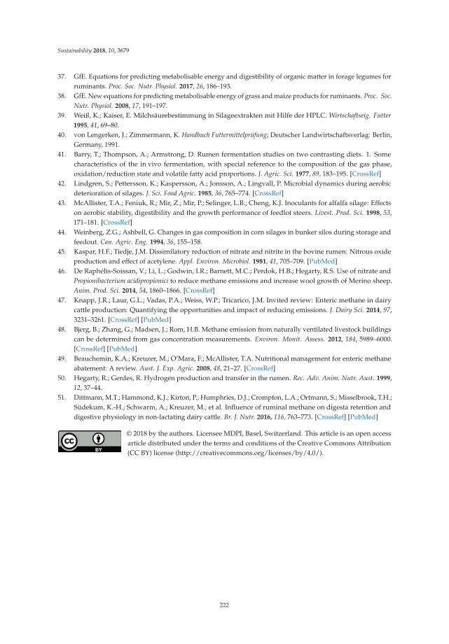
Sustainability 2018, 10, 3679
37. GfE. Equations for predicting metabolisable energy and digestibility of organic matter in forage legumes forruminants. Proc. Soc. Nutr. Physiol. 2017, 26, 186–193.
38. GfE. New equations for predicting metabolisable energy of grass and maize products for ruminants. Proc. Soc.Nutr. Physiol. 2008, 17, 191–197.
39. Weiß, K.; Kaiser, E. Milchsäurebestimmung in Silageextrakten mit Hilfe der HPLC. Wirtschaftseig. Futter1995, 41, 69–80.
40. von Lengerken, J.; Zimmermann, K. Handbuch Futtermittelprüfung; Deutscher Landwirtschaftsverlag: Berlin,Germany, 1991.
41. Barry, T.; Thompson, A.; Armstrong, D. Rumen fermentation studies on two contrasting diets. 1. Somecharacteristics of the in vivo fermentation, with special reference to the composition of the gas phase,oxidation/reduction state and volatile fatty acid proportions. J. Agric. Sci. 1977, 89, 183–195. [CrossRef]
42. Lindgren, S.; Pettersson, K.; Kaspersson, A.; Jonsson, A.; Lingvall, P. Microbial dynamics during aerobicdeterioration of silages. J. Sci. Food Agric. 1985, 36, 765–774. [CrossRef]
43. McAllister, T.A.; Feniuk, R.; Mir, Z.; Mir, P.; Selinger, L.B.; Cheng, K.J. Inoculants for alfalfa silage: Effectson aerobic stability, digestibility and the growth performance of feedlot steers. Livest. Prod. Sci. 1998, 53,171–181. [CrossRef]
44. Weinberg, Z.G.; Ashbell, G. Changes in gas composition in corn silages in bunker silos during storage andfeedout. Can. Agric. Eng. 1994, 36, 155–158.
45. Kaspar, H.F.; Tiedje, J.M. Dissimilatory reduction of nitrate and nitrite in the bovine rumen: Nitrous oxideproduction and effect of acetylene. Appl. Environ. Microbiol. 1981, 41, 705–709. [PubMed]
46. De Raphélis-Soissan, V.; Li, L.; Godwin, I.R.; Barnett, M.C.; Perdok, H.B.; Hegarty, R.S. Use of nitrate andPropionibacterium acidipropionici to reduce methane emissions and increase wool growth of Merino sheep.Anim. Prod. Sci. 2014, 54, 1860–1866. [CrossRef]
47. Knapp, J.R.; Laur, G.L.; Vadas, P.A.; Weiss, W.P.; Tricarico, J.M. Invited review: Enteric methane in dairycattle production: Quantifying the opportunities and impact of reducing emissions. J. Dairy Sci. 2014, 97,3231–3261. [CrossRef] [PubMed]
48. Bjerg, B.; Zhang, G.; Madsen, J.; Rom, H.B. Methane emission from naturally ventilated livestock buildingscan be determined from gas concentration measurements. Environ. Monit. Assess. 2012, 184, 5989–6000.[CrossRef] [PubMed]
49. Beauchemin, K.A.; Kreuzer, M.; O’Mara, F.; McAllister, T.A. Nutritional management for enteric methaneabatement: A review. Aust. J. Exp. Agric. 2008, 48, 21–27. [CrossRef]
50. Hegarty, R.; Gerdes, R. Hydrogen production and transfer in the rumen. Rec. Adv. Anim. Nutr. Aust. 1999,12, 37–44.
51. Dittmann, M.T.; Hammond, K.J.; Kirton, P.; Humphries, D.J.; Crompton, L.A.; Ortmann, S.; Misselbrook, T.H.;Südekum, K.-H.; Schwarm, A.; Kreuzer, M.; et al. Influence of ruminal methane on digesta retention anddigestive physiology in non-lactating dairy cattle. Br. J. Nutr. 2016, 116, 763–773. [CrossRef] [PubMed]
© 2018 by the authors. Licensee MDPI, Basel, Switzerland. This article is an open accessarticle distributed under the terms and conditions of the Creative Commons Attribution(CC BY) license (http://creativecommons.org/licenses/by/4.0/).
222

sustainability
Article
Assessing the Greenhouse Gas Mitigation Effect ofRemoving Bovine Trypanosomiasis in Eastern Africa
Michael MacLeod 1,*, Vera Eory 1 ID , William Wint 2, Alexandra Shaw 3, Pierre J. Gerber 4,5,
Giuliano Cecchi 6 ID , Raffaele Mattioli 7, Alasdair Sykes 1 and Timothy Robinson 7
1 Land Economy, Environment and Society Group, SRUC, Edinburgh EH9 3JG, UK;[email protected] (V.E.); [email protected] (A.S.)
2 Department of Zoology, Environmental Research Group Oxford (ERGO), South Parks Road,Oxford OX1 3PS, UK; [email protected]
3 AP Consultants, 22 Walworth Enterprise Centre, Duke Close, Andover SP10 5AP, UK;[email protected]
4 The World Bank Group, Agriculture and Food Global Practice, 1818 H Street N.W.,Washington, DC 20433, USA; [email protected]
5 Animal Production Systems Group, Wageningen University, P.O. Box 338, Wageningen 6708, The Netherlands6 Food and Agriculture Organization of the United Nations (FAO), Sub-regional Office for Eastern Africa,
CMC Road, P.O. Box 5536, Addis Ababa, Ethiopia; [email protected] Food and Agriculture Organization of the United Nations (FAO), Animal Production and Health Division,
Viale delle Terme di Caracalla, 00153 Rome, Italy; [email protected] (R.M.);[email protected] (T.R.)
* Correspondence: [email protected]; Tel.: +44-131-535-4124
Received: 25 April 2018; Accepted: 15 May 2018; Published: 18 May 2018
Abstract: Increasing the production of meat and milk within sub-Saharan Africa should providesignificant food security benefits. However, greenhouse gas (GHG) emissions represent a challenge,as cattle production in the region typically has high emissions intensity (EI), i.e., high rates of GHGemissions per unit of output. The high EI is caused by the relatively low production efficiencies in theregion, which are in turn partly due to endemic cattle diseases. In theory, improved disease controlshould increase the efficiency and decrease the emissions intensity of livestock production; howeverquantitative analysis of the potential GHG mitigation effects of improved disease control in Africa islacking. This paper seeks to respond to this by using a hybrid modelling approach to quantify theproduction and emissions effects of removing trypanosomiasis from East African cattle productionsystems. The emissions are quantified for each cattle production system using an excel version ofGLEAM, the Food and Agriculture Organization’s Global Livestock Environmental AssessmentModel. The results indicate that removing trypanosomiasis leads to a reduction in the emissionsintensity per unit of protein produced of between 0% and 8%, driven mainly by the increases inmilk yields and cow fertility rates. Despite the limitations, it is argued that the approach providesconsiderable scope for modelling the GHG impacts of disease interventions.
Keywords: cattle health; climate change; livestock modelling; GLEAM; sustainable intensification
1. Introduction
In developing countries growing populations, rising incomes, and urbanization are translatinginto increasing demand for livestock products. Livestock is now one of the fastest growing sub-sectorsof agriculture: a doubling of demand for animal-source foods is expected within developing countriesbetween 2000 and 2050, and a 70% increase for the world as a whole [1,2]. However, it has been notedthat: “Meeting this demand in a way that is socially desirable and environmentally sustainable is amajor challenge facing agriculture today” [3] (p. 9).
Sustainability 2018, 10, 1633; doi:10.3390/su10051633 www.mdpi.com/journal/sustainability223

Sustainability 2018, 10, 1633
A major part of the challenge is the emission of greenhouse gases (GHGs) arising from livestockproduction. It has been estimated through life-cycle assessments that the global livestock sectoraccounts for around 14.5% of all anthropogenic GHG emissions, with cattle meat and milk accountingfor 65% of the livestock emissions [4]. If increased demand is to be met without significant increases inGHG emissions, then ways of reducing the emissions intensity (EI, i.e., the amount of GHG emittedper unit of commodity produced) need to be identified and deployed.
Improving livestock health is potentially a cost-effective way of increasing production,while reducing EI. The World Organisation for Animal Health (OIE) has estimated that: “at theworldwide level, average losses due to animal diseases are more than 20%” [5]. The main directfarm level losses arise from mortality (including involuntary culling), a lowering of the efficiencyof the production process, and reduction in output quantity or quality [6]. Reducing the diseaseburden can lead to significant reductions in EI by, for example, improving the feed conversion ratioof individual animals or changing herd structures (i.e., the proportion of each animal cohort in theherd). However, disease reduction is not yet widely recognised as a mitigation measure [7]. In fact,the Intergovernmental Panel on Climate Change Fifth Assessment Report [8] does not specificallymention livestock health, and current evidence is limited to a small number of studies of Europeanlivestock [9–13].
Understanding the impacts of improving cattle health on production and emissions is of particularrelevance in sub-Saharan Africa (SSA), given that cattle are the predominant source of livestockGHGs [4], growth in demand between 2000 and 2030 is forecast to be 113% for beef and 107% for dairyproducts [1] and that the EIs for bovine milk and meat tend to be higher in SSA than in other regions [14].The higher EIs are largely due to inefficiencies in converting natural resources into edible animalproducts, with relatively high feed conversion ratios and high energy (methane) and nitrogen (nitrousoxide) losses occurring along the process [4]. In these systems, efficiency is closely and positivelyrelated to productivity and key factors such as: milk yield, growth rates, fertility and mortalityrates, and ages at slaughter. These, in turn, are a function of the genetics, feeding, management,environmental stress, and health status of the animals.
While various studies have investigated the effects of improved genetics, feeding, and managementon livestock [15], evidence on the mitigation potential of improving health is scarce. It has been notedthat, “Simulation results seem promising, but reliable quantitative estimates of the mitigation potentialof improved health will require more research” [16] (p. 111). This paper seeks to respond to this byusing a hybrid modelling approach to quantify the production and emissions effects of removingtrypanosomiasis from East African cattle systems.
Trypanosomiasis is a disease caused by tsetse-transmitted parasitic protozoans, and is endemic ina tsetse-infested belt that spans across 9 million square kilometres in SSA [17]. With its animal form(called “nagana”) and its human form (also known as “sleeping sickness”), trypanosomiasis is widelyconsidered as one of the main threats to human and livestock health and agricultural production,and, as such, a major constraint to rural development and poverty alleviation in SSA [18,19]. It hasbeen identified as “the most economically important disease of livestock in sub-Saharan Africa” [20].African trypanosomiasis, in its various forms, can cause a wide range of symptoms, including anaemia,wasting, loss of condition, abortion, and reduced milk production. Progression can lead either to deathor to a chronic form. For many decades chemotherapy has been the mainstay of trypanosomiasiscontrol, but in recent years resistance has emerged as a growing concern [21].
This paper presents a method for quantifying the effect of trypanosomiasis treatment on theproduction and EI of a range of cattle production systems. It quantifies the effect of trypanosomiasistreatment on the EI in East Africa. The limitations of the method are discussed and the wider challengesin quantifying the GHG effects of livestock health improvement are explored.
224

Sustainability 2018, 10, 1633
2. Materials and Methods
2.1. Study Area
The study focuses on East Africa, which is one of the most important dairy development zones inSSA. The specific area of study is the Inter-Governmental Authority on Development (IGAD) region,an area of over 5.2 million km2 that comprises the countries of Djibouti, Eritrea, Ethiopia, Kenya,Somalia, South Sudan, Sudan, and Uganda [22]. Just under half (45%) of the cattle in SSA are reportedto be in the IGAD region [23].
2.2. Cattle Production Systems
The cattle in the study area were classified into twelve distinct production systems (Table 1).These refined cattle systems were based on three main livestock systems (i.e., pastoral, agro-pastoraland mixed farming) [24], which were further disaggregated based on the prevalence of work oxen(used for traction) and milk yields of dairy cattle (which have varying degrees of exotic genetic material,usually of the main European dairy breeds that have been widely adopted in high value smallholderdairy production in Eastern Africa).
Table 1. The 12 cattle production systems analysed, table adapted from [25].
Draft Oxen
Production System
Pastoral Agro-PastoralMixed:
General aMixed:
Ethiopia aHigh MilkYield Dairy
No oxen ×× b
Low oxen × × × ×Medium oxen × × ×
High oxen × × ×a Two mixed farming systems were analysed, one for Ethiopia and one for the other study countries; b High milkyield dairy cows are found in the agro-pastoral and general mixed farming systems.
The high milk yield dairy systems consist of cattle with varying degrees of non-indigenous geneticmaterial derived primarily from the main European dairy breeds, principally Ayrshire, Friesian andChannel Island breeds—Guernsey and Jersey. In the other systems indigenous breeds predominate,i.e., zebu cattle and related crossbreeds [26]. The eastern African indigenous zebu cattle breeds areconventionally divided into three main groups all of which are represented in the countries coveredby this study: the Large East African Zebu (including the Boran breeds of Ethiopia, Kenya andSomalia, the Samburu, Karmajong Zebu, Orma Boran and Butana and Kenana of Sudan) the Small EastAfrican Zebu (including the Maasai, Abyssinian Shorthorned Zebu, Kamba of Kenya and Serere andKyoga in the tsetse-infested areas of Uganda) and the Sanga cattle (including the Ankole of Uganda,Danakil cattle of Ethiopia and the Nuer and Dinka of Sudan). Further information is available on theDomestic Animal Genetic Resources Information System (DAGRIS) [27]. More detail on the productionsystems and how they were defined is available in [28].
Data on the use of work oxen were obtained from in-country informants, reports, census data,livelihood studies [24] and other sources [29–33]. Combining these sources across the region byadministrative area, and studying data on herd compositions, enabled three broad categories of oxenuse to be distinguished depending on the proportion of cattle used for draught: low (≤10%), medium(>10% and <20%), and high (≥20%).
The proportion of cattle modelled in each system is given in Table 2. The most recent statisticsreport a total cattle population in the study area of 144.5m in 2016 [23].
225

Sustainability 2018, 10, 1633
Table 2. The proportion of cattle in each system.
Production System % of Total Cattle Population
Pastoral 12%Agropastoral, low dairy and oxen 34%
Mixed, low dairy and oxen 11%Agropastoral, high dairy and low oxen 2%
Agropastoral, low dairy and medium oxen 1%Agropastoral, low dairy and high oxen 2%
Mixed, high dairy and low oxen 4%Mixed, low dairy and low oxen 1%Mixed, low dairy and high oxen 1%
Mixed, low dairy and medium oxen (eth) 7%Mixed, low dairy and high oxen (eth) 18%Mixed, low dairy and low oxen (eth) 8%
Total 100%
2.3. Modelling Approach
This study builds on previous work, which quantified the economic benefits of removingtrypanosomiasis in East African cattle using the “Mapping the Benefits” (MTB) model [25,28,34].In this study, the MTB model is combined with an excel version of GLEAM (the UN-FAO’s GlobalLivestock Environmental Assessment Model, [35]) which calculates the GHG emissions arising fromproduction. A schematic diagram of the relationship between the models is provided in Figure 1.
Figure 1. Schematic diagram of the relationship between the two models: Mapping the Benefits (MTB)and Global Livestock Environmental Assessment Model (GLEAM).
2.3.1. Harmonising the GLEAM and MTB Herd Models
At the heart of both GLEAM and MTB are herd models, which determine the herd structure andthe number of animals entering and leaving the herd each year. The two herd models perform some ofthese calculations in different ways. For example, they have different animal cohorts (adult female,replacement female, etc.) and different ways of calculating the number of calves born. Therefore,the herd models had to be harmonised, i.e. adjusted until they produced the same herd structure anddynamics. This was achieved by comparing the results given by the two herd models with the sameinput data, and adjusting the calculations in GLEAM until the models were producing the same resultsfor all 12 production systems.
226

Sustainability 2018, 10, 1633
2.3.2. Estimating the Effects of Trypanosomiasis Treatment over 20 Years
The herd structure and dynamics, and the output of meat and milk were calculated for thesituations with and without trypanosomiasis using the MTB model [34] and applied to cattle populationdensity maps, projected using the herd growth and additional spread models. Regional tsetse maps at1 km resolution were used [36], complemented by 5km resolution continental datasets [37] where 1 kmresolution maps were unavailable. Cattle population densities were available from a series of 1kmresolution datasets created within the framework of the IGAD Land Policy Initiative (LPI) using themost recent national statistics available for the period 2000–2005. The mapping methods were thosedeveloped to generate the Gridded Livestock of the World [38].
GLEAM was used to calculate the (meat and milk) production, the total greenhouse gas emissionsarising from that production and the EI of each commodity for each of the cattle systems with andwithout trypanosomiasis. The meat production in live weight was calculated by multiplying thenumber of cattle exiting the herd as offtake, i.e., sold or slaughtered, by the average live weight ofeach cohort (i.e., adult female, calves etc.). The live weight was then converted to edible protein bymultiplying it by (a) the carcass weight: live weight percentage (50–55% depending on the cohort);(b) the bone-free meat: carcass weight percentage (75%) and finally (c) the protein content of bone-freemeat (18%). The edible protein from milk was determined by multiplying the net milk production(milk secreted minus milk suckled) by the protein content of milk (3.3%). Emissions are only allocatedto edible protein and draft, however cattle perform other functions. It has been estimated that 16%of the emissions should be allocated to the manure, financing and dowry functions of cattle [39].Doing so would reduce the EI but would have a negligible impact on the change in EI arising fromtrypanosomiasis removal.
The main GHG-producing activities were included, i.e., the production of feed and fertiliser,the digestion of feed and the excretion of undigested organic matter (Table 3 provides an explanationof the emission categories). The emissions of methane and nitrous oxide were converted to their carbondioxide equivalent using the Intergovernmental Panel on Climate Change (IPCC) global warmingpotentials of 25 and 298, respectively. The system boundary of the study is “cradle to farm-gate”,i.e., emissions arising from the production of feed and other inputs are included but post-farm gateemissions occurring during processing and distribution are not included; however in the systemsstudied post-farm gate emissions are likely to represent a small proportion of the total emissions [4].CO2 emissions and sequestration in short-term carbon cycles (i.e., respiration and photosynthesis)are not included, in keeping with the IPCC guidelines ([40], Volume 4, p. 10.7). Furthermore, it isassumed that the treatment (chemotherapy) has negligible additional GHG emissions arising (fromdrug manufacture and distribution) given the small doses involved. Other treatment strategies, such asthe removal of tsetse habitats, could lead to significant additional GHG emissions.
Table 3. The emission categories quantified in the study.
Category Emissions Sources
Manure N2O Direct and N2O arising from the nitrification/denitrification of excretedN during its management and storage.
Manure CH4CH4 arising from the anaerobic decomposition of excreted organicmatter during its management and storage.
Enteric fermentation CH4 CH4 arising from the microbial decomposition of feed during digestion.
Feed energy CO2
CO2 from: fossil fuel use in the cultivation of feed crops; fossil fuel usein the production of non-crop feed materials; processing, transportationand blending of feed materials; fossil fuel use from the production ofsynthetic fertiliser; land use change arising from soy cultivation.
Feed N2ODirect and indirect N2O from: application of synthetic fertiliser andmanure to crops; crop residue management; direct deposition of N bygrazing animals; fertiliser manufacture.
227

Sustainability 2018, 10, 1633
2.3.3. Parameterising the Cattle Production Systems
The values for the baseline situation (i.e., with trypanosomiasis) in Table 4 were derived fromvarious sources. A few sources provided information relating to all production systems [32,41], others forthe pastoralist systems [42–44], for the agro-pastoral and mixed farming systems [29,31,45–50] and forthe high milk yield “grade” dairy cattle kept in a separate system alongside indigenous cattle in theagro-pastoral and mixed farming systems [51–53].
Table 4. Values for selected parameters used in the analysis (T+ refers to the value with trypanosomiasis,T− to the value without trypanosomiasis). The values were estimated based on a review of longitudinaland cross-sectional studies comparing the productivity observed in infected and uninfected individualcattle or whole herds, under conditions of both high and low trypanosomiasis challenge (see Section 2.3.3).Table adapted from [25].
Parameter
Cattle Production Systems
Pastoral Agro-PastoralMixed Farming
(General)Mixed Farming
(Ethiopia)High Milk Yield
Dairy
T+ T− T+ T− T+ T− T+ T− T+ T−Mortality % of animals dying each yearFemale calves 20 17 18 15 16 13 24 20 21 18Male calves 25 22 20 17 18 15 26 22 26 23
Adult females 7.5 6.5 7.0 6.0 8.0 7.0 9.0 7.5 12.0 10.0Work oxen 9.0 7.2 8.5 6.8 9.0 7.2 10.0 8.0 - -
Fertility % of cows producing a living calf each yearCow fertility 54 58 52 56 51 55 49 54 53 57Lactation Litres of milk per lactation a
Milk offtake 275 296 285 306 300 322 280 301 1900 2042a Lactation length varies depending on the system; in this study it is assumed that most of the milk for humanconsumption is taken off in the 12 months following calving.
The effects of trypanosomiasis treatment on performance were estimated based on a reviewof longitudinal and cross-sectional studies comparing the productivity observed in infected anduninfected individual cattle or whole herds, under conditions of both high and low trypanosomiasischallenge [33,45,54–61]. The review gave a range of values for the effect of the disease. In this study,it was assumed that disease treatment would have an effect between the middle and lower end of therange reported in studies. These (arguably conservative) assumptions were made in order to correctfor the fact that the studies reviewed tended to be conducted in areas where the disease impact wasrelatively severe.
Similar impacts for trypanosomiasis were applied across the production systems (Table 4).This table also shows that baseline cattle mortality rates observed in Eastern Africa tend to be high.This reflects not just the presence of trypanosomiasis, but also of tick-borne diseases, especially EastCoast fever [60] and, locally, very high stocking rates leading to nutritional stress, especially in parts ofthe Ethiopian highlands [62].
2.3.4. Ration Composition and Nutritional Value
The ration (i.e., the livestock feed) for each system was determined using a combination ofapproaches. The proportions of the main feed material categories (i.e., forage, crop residues andconcentrates) were estimated based on literature, expert knowledge, and unpublished surveys,while the percentage of each crop residue (maize, millet and sorghum stover, wheat, rice and barleystraw, and sugar cane tops) were calculated for each cell, based on how much of each crop is producedwithin the cell. Crop data was extracted for livestock production zones from Spatial ProductionAllocation Model (SPAM) V3r6 2000 datasets [63]. The nutritional value of the ration was calculated bymultiplying the nutritional value of each feed material by its proportion in the ration. The nutritional
228

Sustainability 2018, 10, 1633
values of individual feed materials were based on [14,64], the Sub-Saharan Africa Feed CompositionDatabase [65], and Feedipedia [66,67].
2.3.5. Estimating Uncertainty
Calculation of the emission intensities involves parameters that are subject to some degree ofuncertainty. A Monte Carlo simulation was undertaken in order to quantify the uncertainty rangesin the results. Parameters were included in the simulation that were (a) likely to have a significantinfluence on the most important emissions categories (those contributing more than twenty percentof the total emissions, i.e., enteric CH4 and feed N2O) and (b) had a high degree of uncertainty orinherent variability. An initial list of parameters was generated and reviewed. Based on the review,some parameters were excluded, e.g., the emission factors (EFs) for indirect N2O were removed becausevolatilisation and leaching only account for a small % of feed N2O emissions, and a previous study hadfound the contribution to variance of these EFs to be very small (<2%) [14] (p. 81). The distributionsand variability of the parameters are given in Table 5. The variability of forage digestibility is based onthe standard deviation of the digestibility of Napier grass (Pennisetum purpureum) reported in [67].The variability of cow milk yield, cow fertility and calf death rates were based on the ranges reportedin [32]. The Monte Carlo was performed in Model Risk with 5000 runs for each of 12 systems with andwithout trypanosomiasis.
Table 5. Parameters included in the Monte Carlo analysis.
Parameter DistributionCoefficient of
VarianceMinimum-Maximum Basis
Forage digestibility, DE% Normal 6% [67]Milk yield Normal 11–39% [32]
Cow fertility Normal 8–21% [32]Calf death rate Normal 25–45% [32]
Enteric CH4 factor, Ym Normal 10% [40], (Vol. 4, p. 10.33)N2O Emission factor 1 Lognormal 0.003–0.03 [40], (Vol. 4, p. 11.11)N2O Emission factor 3 Lognormal 0.007–0.06 [40], (Vol. 4, p. 11.11)
3. Results
3.1. Baseline Emissions with Trypanosomiasis
The EI by system and emission category is shown in Figure 2. The main sources of emissionsare (a) enteric methane and (b) feed nitrous oxide, i.e., the nitrous oxide arising from the depositionof organic N on pasture (either directly via the urine of grazing animals, or via the spreading ofthe collected manure of housed cattle). The high (milk yield) dairy systems have much lower EIthan other systems due to their higher productivity (where productivity is defined as the mass ofmeat and milk produced by a system each year compared to the live weight mass of the cattle in thesystem). Differences between the other systems are less marked but also largely driven by productivity.The relationship between productivity and EI for the 12 systems with and without trypanosomiasis isshown in Figure 3. This trend is consistent with other studies [68,69] which found a similar relationshipbetween productivity and EI in cattle systems, i.e., large (but reducing) marginal decreases in EI withincreasing productivity in low productivity systems, such as those in East Africa.
229
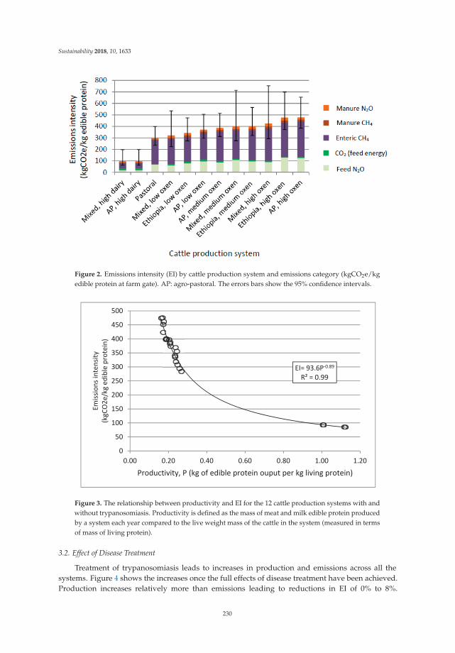
Sustainability 2018, 10, 1633
Figure 2. Emissions intensity (EI) by cattle production system and emissions category (kgCO2e/kgedible protein at farm gate). AP: agro-pastoral. The errors bars show the 95% confidence intervals.
Figure 3. The relationship between productivity and EI for the 12 cattle production systems with andwithout trypanosomiasis. Productivity is defined as the mass of meat and milk edible protein producedby a system each year compared to the live weight mass of the cattle in the system (measured in termsof mass of living protein).
3.2. Effect of Disease Treatment
Treatment of trypanosomiasis leads to increases in production and emissions across all thesystems. Figure 4 shows the increases once the full effects of disease treatment have been achieved.Production increases relatively more than emissions leading to reductions in EI of 0% to 8%.
230

Sustainability 2018, 10, 1633
The reductions in EI are significant in eleven of the twelve systems and are closely (inversely) correlatedwith the change in productivity (Figure 5).
Figure 4. Difference in total edible protein production and GHG emissions with disease treatment.AP: agro-pastoral.
Figure 5. Change in EI and productivity with disease treatment. EI is measured in terms of kgCO2eper kg of edible protein produced and productivity. Productivity is defined as the mass of meat andmilk edible protein produced by a system each year compared to the live weight mass of the cattlein the system (measured in terms of mass of living protein). (Key: a1 = agro-pastoral high dairy;a2 = agro-pastoral low dairy, high oxen; a3 = agro-pastoral low dairy, medium oxen; a4 = agro-pastorallow dairy, low oxen; m1 = mixed high dairy; m2 = mixed low dairy, high oxen; m3 = mixed low dairy,medium oxen; m4 = mixed, low dairy, low oxen; e1 = Ethiopia low dairy, high oxen; e2 = Ethiopia lowdairy, medium oxen; e3 = Ethiopia, low dairy, low oxen; p = pastoral.).
231

Sustainability 2018, 10, 1633
3.3. Factors driving the Changes in EI
A sensitivity analysis was undertaken in order to investigate the influence of different parameterson EI (Table 6). The EI is highly sensitive to changes in the digestibility of forage, and to the entericmethane emission factor (Ym), however, both of these remain constant with changes in disease status.Increased milk yield leads to a decrease in EI as a greater percentage of the lactating cow’s feed energyrequirement is used for the production of edible outputs (i.e., lactation) rather than non-productiveactivity (e.g., maintenance or locomotion), [68]. The increased cow fertility rate leads to a higherproportion of the adult females producing edible outputs. This is important as while non-lactatingadult females produce lower emissions than lactating ones, they produce no edible outputs (i.e., milkor liveweight gain) so their EI is effectively infinite. The increased fertility rate also changes theherd structure, but this has a limited effect on EI. EI is less sensitive to changes in calf mortalitythan it is to changes in cow milk yield or fertility, however the effect of calf mortality on EI dependson the fate of the dying calves, i.e., what proportion enter the human food chain and are thereforecounted as production. Finally, increasing the use of draft oxen leads to increases EI in some systems.Draft animals have a high EI as they produce no/limited edible output, so even when a proportion ofthe emissions are allocated to labour, they still have a higher EI than younger, faster growing cattle.
Table 6. Summary of the sensitivity analysis, showing the change in EI resulting from a ±10% changein each parameter (“Draft”: the % of male cattle aged >3 years old that are used for draft. EF: emissionfactor; DE: digestible energy).
System Change inParameter
Change in EI
Constant Vary with System Vary with System and Disease Status
N2OEF1
N2OEF3
ForageDE%
EntericCH4, Ym
MilkYield
CowFertility
Calf DeathRate
Draft
Pastoral +10% 0.7% 1.2% −16.4% 7.2% −4.5% −3.9% −0.6% 0.5%Pastoral −10% −0.7% −1.2% 23.1% −7.2% 4.9% 4.9% 0.6% −0.5%
AP, high dairy +10% 1.6% 0.1% −15.8% 5.1% −6.3% −5.4% 2.2% 0.0%AP, high dairy −10% −1.6% −0.1% 22.2% −5.1% 7.5% 6.7% 0.0% 0.0%AP, low oxen +10% 1.4% 0.7% −16.4% 6.3% −4.4% −2.9% −0.7% 1.0%AP, low oxen −10% −1.4% −0.7% 23.5% −6.3% 4.8% 3.5% 0.7% −1.0%
AP, medium oxen +10% 1.1% 0.7% −16.5% 6.8% −4.4% −3.0% −0.7% 2.0%AP, medium oxen −10% −1.1% −0.7% 23.7% −6.8% 4.8% 3.6% 0.7% −2.0%
AP, high oxen +10% 1.3% 0.7% −16.3% 6.5% −4.4% −3.1% −0.7% 3.8%AP, high oxen −10% −1.3% −0.7% 23.3% −6.5% 4.9% 3.9% 0.7% −3.8%
Mixed, high dairy +10% 1.6% 0.1% −15.8% 5.1% −6.3% −5.4% 2.3% 0.0%Mixed, high dairy −10% −1.6% −0.1% 22.2% −5.1% 7.5% 6.7% −0.1% 0.0%Mixed, low oxen +10% 1.2% 0.3% −17.1% 6.7% −4.4% −1.7% −0.9% 0.9%Mixed, low oxen −10% −1.2% −0.3% 24.9% −6.7% 4.9% 2.0% 0.9% −0.9%
Mixed, medium oxen +10% 1.8% 0.3% −16.7% 6.2% −4.5% −2.7% −0.6% 2.0%Mixed, medium oxen −10% −1.8% −0.3% 24.1% −6.2% 4.9% 3.7% 0.6% −2.0%
Mixed, high oxen +10% 1.4% 0.3% −16.8% 6.7% −4.5% −3.3% −0.6% 3.8%Mixed, high oxen −10% −1.4% −0.3% 24.3% −6.7% 4.9% 4.1% 0.6% −3.7%
Ethiopia, low oxen +10% 1.5% 0.3% −16.8% 6.4% −4.5% −1.7% −1.5% 0.6%Ethiopia, low oxen −10% −1.5% −0.3% 24.5% −6.4% 5.0% 2.0% 1.5% −0.6%
Ethiopia, medium oxen +10% 1.6% 0.3% −16.8% 6.4% −4.6% −3.1% −1.1% 2.0%Ethiopia, medium oxen −10% −1.6% −0.3% 24.3% −6.4% 5.1% 3.7% 1.0% −2.0%
Ethiopia, high oxen +10% 1.8% 0.3% −16.6% 6.2% −4.6% −3.5% −1.0% 3.7%Ethiopia, high oxen −10% −1.8% −0.3% 23.9% −6.2% 5.1% 4.3% 0.9% −3.6%
4. Discussion
While the results are consistent with the expectation that improving health is likely to lead toreductions in EI, the validity of the results depends on the input assumptions and the method used toperform the calculations. The approach developed in this study allows multiple effects of a diseaseto be quantified. The MTB model enables herd growth and livestock movement over time to bequantified. The use of a herd model in GLEAM enables disease impacts on parameters that affectthe herd structure to be modelled, e.g. death rates, fertility rates, replacement rates, and offtakerates. The IPCC tier 2 approach [40] to calculating livestock emissions used in GLEAM enablesdisease impacts on parameters that affect the production and emissions of the individual animal to
232

Sustainability 2018, 10, 1633
be modelled, e.g., milk yield, animal growth rates, activity level and ration. However, the approachrequires further development in order to capture some potentially important effects, such as the impactof disease status on ration quality.
The results are expressed in terms of the functional unit “kg of CO2e per kg of edible protein atthe farm gate”, and therefore don’t include post-farm emissions or take into account post-farm losses.While post-farm emissions are likely to represent a small % of the total emissions, losses can makesignificant differences to the EI, and may vary between different production systems. The functionalunit also assumes that: (a) 1 kg of milk protein is equivalent to 1 kg of meat protein and (b) productionof edible outputs is the only reason for keeping cattle, which are simplifications. Although some ofthe emissions are allocated to draught power, none are allocated to other outputs (such as manure)or the less tangible values that cattle may have, such as social value and increased resilience of theirowners [39]. While the choice of functional unit means that care needs to be taken when makingcomparisons of the EI between systems, none of the limitations noted above would affect the changein EI arising from treatment of trypanosomiasis.
As noted in [25] “data on livestock productivity (fertility, mortality, milk yields and output ofdraught power) were mostly obtained from a limited number of in-depth studies in specific localities.As the large number of references testifies, cattle systems in the study region have been much studiedand there is enough information to paint a good general picture, and to cross-check and validate.However, although trypanosomosis has been relatively well researched, there remains a need formore specific studies on this disease’s impact”. This is particularly the case with draught animals.FAO have developed a geospatial database [70] that should improve understanding of trypanosomiasisprevalence in Africa.
5. Conclusions
The treatment of trypanosomiasis in East African cattle systems could lead to reductions in EIof between 0 and 8%, depending on the system. EI is closely related to productivity, and the largestreductions in EI are in those systems experiencing the largest increases in productivity, i.e., the higher(milk yield) dairy systems. However, when making inter-system comparisons, it should be borne inmind that in some systems cattle perform functions in addition to producing meat and milk.
The approach employed in this study could, in principle, be used to model the impact of otherimportant diseases in SSA (such as foot and mouth disease), if their effects can be adequately describedin terms of the model parameters. However, in order to produce valid results, the main direct effectsof the disease need to be captured by the model. This is potentially challenging given the lack of dataon prevalence and impact for many diseases. While it may be possible to partially fill gaps through theanalysis of existing datasets (such as abattoir records), some diseases have important effects that arenot routinely recorded or readily measured (for example they may alter feed intake, the efficiency ofdigestion or energy partitioning) and may require bespoke studies. A second challenge is capturingthe indirect effects of disease control. For example, disease treatment would lead to increased livestockpopulations which could, depending on how this increase is managed, lead to overstocking and thusreduced feed availability and/or quality.
The reduction of EI represents an external benefit of disease control, i.e., it is a benefit not normallyfactored into farm management or policy decisions. In order to achieve the economically optimallevel of disease control, such externalities need to be quantified and included in decision making,alongside other costs and benefits. Given the difficulty of measuring agricultural GHG emissionsdirectly, it is suggested that modelling approaches, such as the one outlined in this paper, have animportant contribution to make to the development of disease control strategies.
Author Contributions: Conceptualization, M.M. and T.R.; Data curation, M.M., W.W., and A.S.; Formal analysis,M.M. and A.S.; Funding acquisition, T.R.; Investigation, V.E., W.W., A.S., P.G., G.C., and R.M.; Methodology, M.M.;Writing—original draft, M.M.
233
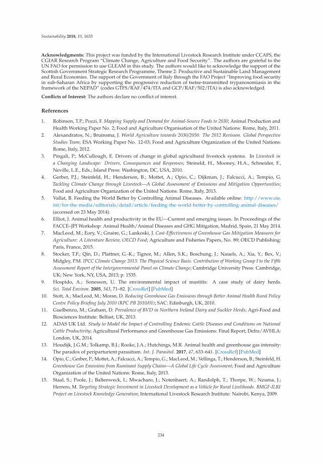
Sustainability 2018, 10, 1633
Acknowledgments: This project was funded by the International Livestock Research Institute under CCAFS, theCGIAR Research Program “Climate Change, Agriculture and Food Security”. The authors are grateful to theUN FAO for permission to use GLEAM in this study. The authors would like to acknowledge the support of theScottish Government Strategic Research Programme, Theme 2: Productive and Sustainable Land Managementand Rural Economies. The support of the Government of Italy through the FAO Project “Improving food securityin sub-Saharan Africa by supporting the progressive reduction of tsetse-transmitted trypanosomiasis in theframework of the NEPAD” (codes GTFS/RAF/474/ITA and GCP/RAF/502/ITA) is also acknowledged.
Conflicts of Interest: The authors declare no conflict of interest.
References
1. Robinson, T.P.; Pozzi, F. Mapping Supply and Demand for Animal-Source Foods to 2030; Animal Production andHealth Working Paper No. 2; Food and Agriculture Organisation of the United Nations: Rome, Italy, 2011.
2. Alexandratos, N.; Bruinsma, J. World Agriculture towards 2030/2050. The 2012 Revision. Global PerspectiveStudies Team; ESA Working Paper No. 12-03; Food and Agriculture Organization of the United Nations:Rome, Italy, 2012.
3. Pingali, P.; McCullough, E. Drivers of change in global agricultural livestock systems. In Livestock ina Changing Landscape: Drivers, Consequences and Responses; Steineld, H., Mooney, H.A., Schneider, F.,Neville, L.E., Eds.; Island Press: Washington, DC, USA, 2010.
4. Gerber, P.J.; Steinfeld, H.; Henderson, B.; Mottet, A.; Opio, C.; Dijkman, J.; Falcucci, A.; Tempio, G.Tackling Climate Change through Livestock—A Global Assessment of Emissions and Mitigation Opportunities;Food and Agriculture Organization of the United Nations: Rome, Italy, 2013.
5. Vallat, B. Feeding the World Better by Controlling Animal Diseases. Available online: http://www.oie.int/for-the-media/editorials/detail/article/feeding-the-world-better-by-controlling-animal-diseases/(accessed on 23 May 2014).
6. Elliot, J. Animal health and productivity in the EU—Current and emerging issues. In Proceedings of theFACCE–JPI Workshop: Animal Health/Animal Diseases and GHG Mitigation, Madrid, Spain, 21 May 2014.
7. MacLeod, M.; Eory, V.; Gruère, G.; Lankoski, J. Cost-Effectiveness of Greenhouse Gas Mitigation Measures forAgriculture: A Literature Review, OECD Food; Agriculture and Fisheries Papers, No. 89; OECD Publishing:Paris, France, 2015.
8. Stocker, T.F.; Qin, D.; Plattner, G.-K.; Tignor, M.; Allen, S.K.; Boschung, J.; Nauels, A.; Xia, Y.; Bex, V.;Midgley, P.M. IPCC Climate Change 2013: The Physical Science Basis. Contribution of Working Group I to the FifthAssessment Report of the Intergovernmental Panel on Climate Change; Cambridge University Press: Cambridge,UK; New York, NY, USA, 2013; p. 1535.
9. Hospido, A.; Sonesson, U. The environmental impact of mastitis: A case study of dairy herds.Sci. Total Environ. 2005, 343, 71–82. [CrossRef] [PubMed]
10. Stott, A.; MacLeod, M.; Moran, D. Reducing Greenhouse Gas Emissions through Better Animal Health Rural PolicyCentre Policy Briefing July 2010 (RPC PB 2010/01); SAC: Edinburgh, UK, 2010.
11. Guelbenzu, M.; Graham, D. Prevalence of BVD in Northern Ireland Dairy and Suckler Herds; Agri-Food andBiosciences Institute: Belfast, UK, 2013.
12. ADAS UK Ltd. Study to Model the Impact of Controlling Endemic Cattle Diseases and Conditions on NationalCattle Productivity; Agricultural Performance and Greenhouse Gas Emissions: Final Report; Defra/AVHLA:London, UK, 2014.
13. Houdijk, J.G.M.; Tolkamp, B.J.; Rooke, J.A.; Hutchings, M.R. Animal health and greenhouse gas intensity:The paradox of periparturient parasitism. Int. J. Parasitol. 2017, 47, 633–641. [CrossRef] [PubMed]
14. Opio, C.; Gerber, P.; Mottet, A.; Falcucci, A.; Tempio, G.; MacLeod, M.; Vellinga, T.; Henderson, B.; Steinfeld, H.Greenhouse Gas Emissions from Ruminant Supply Chains—A Global Life Cycle Assessment; Food and AgricultureOrganization of the United Nations: Rome, Italy, 2013.
15. Staal, S.; Poole, J.; Baltenweck, I.; Mwacharo, J.; Notenbaert, A.; Randolph, T.; Thorpe, W.; Nzuma, J.;Herrero, M. Targeting Strategic Investment in Livestock Development as a Vehicle for Rural Livelihoods. BMGF-ILRIProject on Livestock Knowledge Generation; International Livestock Research Institute: Nairobi, Kenya, 2009.
234

Sustainability 2018, 10, 1633
16. Hristov, A.N.; Oh, J.; Lee, C.; Meinen, R.; Montes, F.; Ott, T.; Firkins, J.; Rotz, A.; Dell, C.; Adesogan, A.;et al. Mitigation of Greenhouse Gas Emissions in Livestock Production—A Review of Technical Options for Non-CO2
Emissions; Gerber, P.J., Henderson, B., Makkar, H.P.S., Eds.; FAO Animal Production and Health PaperNo. 177; Food and Agriculture Organization of the United Nations: Rome, Italy, 2013.
17. Cecchi, G.; Mattioli, R.; Slingenbergh, J.; De La Rocque, S. Land cover and tsetse fly distributions insub-Saharan Africa. Med. Vet. Entomol 2008, 22, 364–373. [CrossRef] [PubMed]
18. Cattand, P.; Simarro, P.; Jannin, J.; Ly, C.; Fall, A.; Shaw, A.; Mattioli, R. Linking Sustainable Human andAnimal African Trypanosomiasis Control with Rural Development Strategies; Programme Against AfricanTrypanosomiasis–Technical and Scientific Series. Vol. 10. 2010; Food and Agriculture Organization ofthe United Nations: Rome, Italy, 2010.
19. Simarro, P.P.; Cecchi, G.; Franco, J.R.; Paone, M.; Diarra, A.; Ruiz-Postigo, J.A.; Fèvre, E.M.; Mattioli, R.;Jannin, J.G. Estimating and mapping the population at risk of sleeping sickness. PLoS Negl. Trop. Dis. 2012,6, 1859. [CrossRef] [PubMed]
20. Taylor, K.; Authié, E.M.-L. Pathogenesis of Animal Trypanosomiasis. In The Trypanosomiases; Maudlin, I.,Holmes, P.H., Miles, M.A., Eds.; CAB International: Wallingford, UK, 2004.
21. Diall, O.; Cecchi, G.; Wanda, G.; Argilés-Herrero, R.; Vreysen, M.J.B.; Cattoli, G.; Viljoen, G.J.; Mattioli, R.;Bouyer, J. Developing a Progressive Control Pathway for African Animal Trypanosomosis. Trends Parasitol.2017, 33, 499–509. [CrossRef] [PubMed]
22. IGAD. The IGAD Region. Available online: https://igad.int/index.php/about-us/the-igad-region (accessedon 24 September 2017).
23. FAOSTAT Live Animals. Available online: http://www.fao.org/faostat/en/#data/QA (accessed on 9 May 2018).24. Cecchi, G.; Wint, W.; Shaw, A.; Marletta, A.; Mattioli, R.; Robinson, T. Geographic distribution and
environmental characterization of livestock production systems in Eastern Africa. Agric. Ecosyst. Environ.2010, 135, 98–110. [CrossRef]
25. Shaw, A.P.M.; Cecchi, G.; Wint, G.R.W.; Mattioli, R.C.; Robinson, T.P. Mapping the economic benefits ofintervening against bovine trypanosomiasis in Eastern Africa. Prev. Vet. Med. 2014, 113, 197–210. [CrossRef][PubMed]
26. Mwai, O.; Hanotte, O.; Kwon, Y.-J.; Cho, S. African Indigenous Cattle: Unique Genetic Resources in a RapidlyChanging World. Asian-Australas. J. Anim. Sci. 2015, 28, 911–921. [CrossRef] [PubMed]
27. Domestic Animal Genetic Resources Information System (DAGRIS). Available online: http://dagris.info/(accessed on 9 May 2018).
28. Shaw, A.; Wint, W.; Cecchi, G.; Torr, S.; Waiswa, C.; Alemu, T.; Eregae, M.; Abdi, A.; Muchina, S.; Mugasi, S.;et al. Intervening against Bovine Trypanosomosis in Eastern Africa: Mapping the Costs and Benefits; PAAT Technicaland Scientific Series No. 11; FAO: Rome, Italy, 2017; Available online: http://www.fao.org/3/a-i7342e.pdf(accessed on 15 May 2018).
29. Itty, P. Economics of Village Cattle Production in Tsetse-affected Areas of Africa. In A Study of TrypanosomiasisControl Using Trypanotolerant Cattle and Chemotherapy in Ethiopia, Kenya, The Gambia, Côte d’Ivoire, Zaire andTogo; Hartung-Gorre Verlag: Constance, Germany, 1992.
30. Starkey, P.; Kaumbutho, P. Meeting the Challenges of Animal Traction. In A Resource Book of the AnimalTraction Network for East-ern and Southern Africa (ATNESA), Harare, Zimbabwe; Intermediate TechnologyPublications: London, UK, 1999.
31. Rege, J.E.O.; Kahi, A.K.; Okomo-Adhiambo, M.; Mwacharo, J.; Hanotte, O. Zebu Cattle of Kenya: Uses,Performance, Farmer Preferences, Measures of Genetic Diversity; ILRI (International Livestock Research Institute)and Kenya Agriculture Research Institute (KARI): Nairobi, Kenya, 2001.
32. Otte, M.J.; Chilonda, P. Cattle and Small Ruminant Production Systems in Sub-Saharan Africa. A SystematicReview; FAO (Food and Agriculture Organization of the United Nations): Rome, Italy, 2002.
33. Ocaido, M.; Otim, C.; Okuna, N.; Erume, J.; Ssekitto, C.; Wafula, R.; Kakaire, D.; Walubengo, J.; Monrad, J.Socio-economic and livestock disease survey of agro-pastoral communities in Serere County, Soroti District,Uganda. Livest. Res. Rural Dev. 2005, 17, 93.
34. Shaw, A.P.M.; Wint, G.R.W.; Cecchi, G.; Torr, S.J.; Mattioli, R.C.; Robinson, T.P. Mapping the benefit-costratios of interventions against bovine trypanosomiasis in Eastern Africa. Prev. Vet. Med. 2015, 122, 406–416.[CrossRef] [PubMed]
235

Sustainability 2018, 10, 1633
35. MacLeod, M.J.; Vellinga, T.; Opio, C.; Falcucci, A.; Tempio, G.; Henderson, B.; Makkar, H.; Mottet, A.;Robinson, T.; Steinfeld, H.; et al. Invited Review: A Position on the Global Livestock EnvironmentalAssessment Model (GLEAM). Animal 2018, 12, 383–397. [CrossRef] [PubMed]
36. Wint, G.R.W. Kilometre Resolution Tsetse Fly Distribution Maps for the Lake Victoria Basin and West Africa; Reportto the Joint Food and Agriculture Organization of the United Nations/International Atomic Energy AgencyProgramme; Food and Agriculture Organization: Rome, Italy, 2001.
37. Wint, W.; Rogers, D. Predicted Distributions of Tsetse in Africa; Report of the Environmental Research GroupOxford Ltd and TALA Research Group, Department of Zoology, University of Oxford, for the Animal HealthService of the Animal Production and Health Division of the Food and Agriculture Organisation of theUnited Nations; FAO: Rome, Italy, 2000.
38. Wint, W.; Robinson, T. Gridded Livestock of the World; FAO (Food and Agricultural Organization of the UnitedNations): Rome, Italy, 2007.
39. Weiler, V.; Udo, H.M.; Viets, T.; Crane, T.A.; De Boer, I.J. Handling multi-functionality of livestock in a lifecycle assessment: The case of smallholder dairying in Kenya. Curr. Opin. Environ. Sustain. 2014, 8, 29–38.[CrossRef]
40. IPCC. IPCC Guidelines for National Greenhouse Gas Inventories; Prepared by the National Greenhouse GasInventories Programme; Eggleston, H.S., Buendia, L., Miwa, K., Ngara, T., Tanabe, K., Eds.; IPCC: Kanagawa,Japan, 2006.
41. Peeler, E.; Omore, A. Manual of Livestock Production Systems in Kenya; KARI (Kenya Agricultural ResearchInstitute): Nairobi, Kenya, 1997.
42. Roderick, S.; Stevenson, P.; Mwendia, C.; Okech, G. The use of trypanocides and antibiotics by Maasaipastoralists. Trop. Anim. Health Prod. 2000, 32, 361–374. [CrossRef] [PubMed]
43. Roderick, S.; Stevenson, P.; Ndungu, J. The production parameters influencing the composition and structureof pastoral cattle herds in a semi-arid area of Kenya. Anim. Sci. 1998, 66, 585–594. [CrossRef]
44. Roderick, S.; Stevenson, P.; Ndungu, J. Factors influencing the production of milk from pastoral cattle herdsin Kenya. Anim. Sci. 1999, 68, 201–209.
45. Itty, P.; Swallow, B.; Rowlands, G.; Mulatu, W.; d’Ieteren, G. The economics of village cattle production in atsetse-infested area of southwest Ethiopia. Prev. Vet. Med. 1995, 22, 183–196. [CrossRef]
46. Swallow, B. Impacts of Trypanosomiasis on African Agriculture; Food and Agriculture Organization of theUnited Nations (FAO): Rome, Italy, 2000.
47. Muraguri, G.R. Epidemiological and Financial Impact of Vector-borne Diseases on Productivity of Smallholder Cattlein the Coastal Lowlands of Kenya; Department of Agriculture, University of Reading: Reading, UK, 2000; p. 219.
48. Machila, N. Improved Targeting and Appropriate Use of Trypanocidal Drugs for the Control of African BovineTrypanosomiasis in Tsetse Endemic Areas of Western and Coastal Kenya within the Context of Primary VeterinaryCare; University of Edinburgh: Edinburgh, UK, 2005; p. 304.
49. Musa, L.; Peters, K.; Ahmed, M. On farm characterization of Butana and Kenana cattle breed productionsystems in Sudan. Livest. Res. Rural Dev. 2006, 18, 177.
50. Maichomo, M.; Ndungu, J.; Ngare, P.; Ole-Mapenay, I. The performance of Orma Boran and Maasai Zebucrossbreeds in a trypanosomiasis endemic area of Nguruman, south western Kenya. Onderstepoort J. Vet. Res.2010, 72, 87–93.
51. Omore, A.; Muriuki, H.; Kenyanjui, M.; Owango, M.; Staal, S. The Kenyan Dairy Sub-Sector: A Rapid Appraisal;Smallholder Dairy (Research & Development) Project Report; ILRI (International Live-stock ResearchInstitute): Nairobi, Kenya, 1999.
52. Mudavadi, P.O.; Otieno, K.J.; Wanambacha, W.; Odenya, J.O.; Odendo, M.; Njaro, O.K. Smallholder DairyProduction and Marketing in Western Kenya: A Review of Literature; Smallholder Dairy (Research & Development)Project Research Report; ILRI (International Livestock Research Institute): Nairobi, Kenya, 2001.
53. Ongadi, P.; Wakhungu, J.; Wahome, R.; Okitoi, L. Characterization of grade dairy cattle owning householdsin mixed small scale farming systems of Vihiga, Kenya. Livest. Res. Rural Dev. 2007, 19, 43.
54. Fox, R.G.R.; Mmbando, S.; Fox, M.; Wilson, A. Effect on herd health and productivity of controlling tsetse andtrypanosomiasis by applying deltamethrin to cattle. Trop. Anim. Health Prod. 1993, 25, 203–214. [CrossRef][PubMed]
55. Jemal, A.; Hugh-Jones, M.E. Association of tsetse control with health and productivity of cattle in the DidessaValley, western Ethiopia. Prev. Vet. Med. 1995, 22, 29–40. [CrossRef]
236

Sustainability 2018, 10, 1633
56. Laker, C.D. Assessment of the Economic Impact of Bovine Trypanosomiasis and its Control in Dairy Cattle in MukonoCounty, Uganda; Makerere University: Kampala, Uganda, 1998.
57. Rowlands, G.; Mulatu, W.; Leak, S.; Nagda, S.; d’Ieteren, G. Estimating the effects of tsetse control onlivestock productivity—A case study in southwest Ethiopia. Trop. Anim. Health Prod. 1999, 31, 279–294.[CrossRef] [PubMed]
58. Shaw, A. Economics of African trypanosomiasis. In The Trypanosomiases; Maudlin, I., Holmes, P., Miles, M., Eds.;CABI Publishing: Wallingford, UK, 2004; pp. 369–402.
59. Mugunieri, G.; Matete, G. Association of trypanosomiasis risk with dairy cattle production in western Kenya.Onderstepoort J. Vet. Res. 2005, 72, 279–284. [CrossRef] [PubMed]
60. Minjauw, B.; McLeod, A. Tick-borne Diseases and Poverty; DFID Animal Health Programme: Edinburgh,UK, 2003.
61. Tesfaye, D.; Speybroeck, N.; De Deken, R.; Thys, E. Economic burden of bovine trypanosomiasis in threevillages of Metekel zone, Northwest Ethiopia. Trop. Anim. Health Prod. 2012, 44, 873–879. [CrossRef][PubMed]
62. Wilson, R.T.; Bech, J.N.; Waveren, E. Draught animals in the livelihoods of mixed smallholder farmers inNorth Wollo, Ethiopia. Draught Anim. News 2002, 37, 2–8.
63. You, L.; Guo, Z.; Koo, J.; Sebastian, K.; Wood-Sichra, U. Spatial Production Allocation Model (SPAM) 2005Version 1; Provided through Harvest Choice; International Food Policy Research Institute: Washington,DC, USA; University of Minnesota: St. Paul, MN, USA, 2014; Available online: http://harvestchoice.org(accessed on 8 January 2015).
64. Lukuyu, B.; Gachuiri, C.K.; Lukuyu, M.N.; Lusweti, C.; Mwendia, S. Feeding Dairy Cattle in East Africa; EastAfrica Dairy Development Project: Nairobi, Kenya, 2012.
65. CGIAR/ILRI Sub-Saharan Africa Feed Composition Database. Available online: http://192.156.137.110/ssafeed/ (accessed on 1 December 2015).
66. Feedipedia. Feedipedia Animal Feed Resources Information System, a Programme by INRA, CIRAD, AFZand FAO. Available online: http://www.feedipedia.org (accessed on 1 August 2015).
67. Feedipedia Napier Grass. Available online: https://www.feedipedia.org/node/395 (accessed on13 December 2017).
68. Capper, J.L.; Cady, R.A.; Bauman, D.E. The environmental impact of dairy production: 1944 compared with2007. J. Anim. Sci. 2009, 87, 2160–2167. [CrossRef] [PubMed]
69. Gerber, P.; Vellinga, T.; Opio, C.; Steinfeld, H. Productivity gains and greenhouse gas EI in dairy systems.Livest. Sci. 2011, 139, 100–108. [CrossRef]
70. Cecchi, G.; Paone, M.; Feldmann, U.; Vreysen, M.J.B.; Diall, O.; Mattioli, R.C. Assembling a geospatialdatabase of tsetse-transmitted animal trypanosomiasis for Africa. Parasites Vectors 2014, 7, 39. [CrossRef][PubMed]
© 2018 by the authors. Licensee MDPI, Basel, Switzerland. This article is an open accessarticle distributed under the terms and conditions of the Creative Commons Attribution(CC BY) license (http://creativecommons.org/licenses/by/4.0/).
237
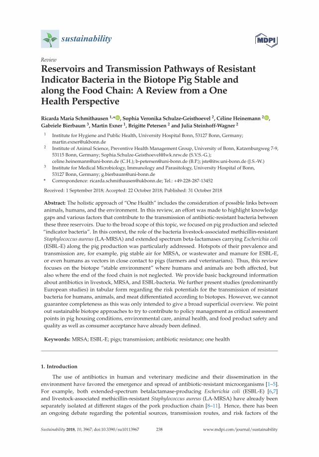
sustainability
Review
Reservoirs and Transmission Pathways of ResistantIndicator Bacteria in the Biotope Pig Stable andalong the Food Chain: A Review from a OneHealth Perspective
Ricarda Maria Schmithausen 1,* , Sophia Veronika Schulze-Geisthoevel 2, Céline Heinemann 2 ,
Gabriele Bierbaum 3, Martin Exner 1, Brigitte Petersen 2 and Julia Steinhoff-Wagner 2
1 Institute for Hygiene and Public Health, University Hospital Bonn, 53127 Bonn, Germany;[email protected]
2 Institute of Animal Science, Preventive Health Management Group, University of Bonn, Katzenburgweg 7-9,53115 Bonn, Germany; [email protected] (S.V.S.-G.);[email protected] (C.H.); [email protected] (B.P.); [email protected] (J.S.-W.)
3 Institute for Medical Microbiology, Immunology and Parasitology, University Hospital of Bonn,53127 Bonn, Germany; [email protected]
* Correspondence: [email protected]; Tel.: +49-228-287-13452
Received: 1 September 2018; Accepted: 22 October 2018; Published: 31 October 2018
Abstract: The holistic approach of “One Health” includes the consideration of possible links betweenanimals, humans, and the environment. In this review, an effort was made to highlight knowledgegaps and various factors that contribute to the transmission of antibiotic-resistant bacteria betweenthese three reservoirs. Due to the broad scope of this topic, we focused on pig production and selected“indicator bacteria”. In this context, the role of the bacteria livestock-associated methicillin-resistantStaphylococcus aureus (LA-MRSA) and extended spectrum beta-lactamases carrying Escherichia coli(ESBL-E) along the pig production was particularly addressed. Hotspots of their prevalence andtransmission are, for example, pig stable air for MRSA, or wastewater and manure for ESBL-E,or even humans as vectors in close contact to pigs (farmers and veterinarians). Thus, this reviewfocuses on the biotope “stable environment” where humans and animals are both affected, butalso where the end of the food chain is not neglected. We provide basic background informationabout antibiotics in livestock, MRSA, and ESBL-bacteria. We further present studies (predominantlyEuropean studies) in tabular form regarding the risk potentials for the transmission of resistantbacteria for humans, animals, and meat differentiated according to biotopes. However, we cannotguarantee completeness as this was only intended to give a broad superficial overview. We pointout sustainable biotope approaches to try to contribute to policy management as critical assessmentpoints in pig housing conditions, environmental care, animal health, and food product safety andquality as well as consumer acceptance have already been defined.
Keywords: MRSA; ESBL-E; pigs; transmission; antibiotic resistance; one health
1. Introduction
The use of antibiotics in human and veterinary medicine and their dissemination in theenvironment have favored the emergence and spread of antibiotic-resistant microorganisms [1–5].For example, both extended-spectrum betalactamase-producing Escherichia coli (ESBL-E) [6,7]and livestock-associated methicillin-resistant Staphylococcus aureus (LA-MRSA) have already beenseparately isolated at different stages of the pork production chain [8–11]. Hence, there has beenan ongoing debate regarding the potential sources, transmission routes, and risk factors of the
Sustainability 2018, 10, 3967; doi:10.3390/su10113967 www.mdpi.com/journal/sustainability238

Sustainability 2018, 10, 3967
continuous spread of MRSA and ESBL-E between animals, humans, and the environment [12–16].Thus, they are also perceived as a potential threat to public health [17–23]. Therefore, in this review,methicillin-resistant Staphylococcus aureus (MRSA) and ESBL-E have been used as “indicator” bacteriawith possible zoonotic potential and occurrence in both the stable biotopes and healthcare sectorand community [24]. Consequently, farmers have been confronted with several consequences of thisproblem: The potential danger of animal colonization with drug-resistant bacteria for (i) humans livingon or in the vicinity of farms [25–27], and (ii) for consumers of animal products [3,28–31]. The intendedaudience of this review is farmers of intensive pig production systems worldwide as well as healthcareworkers, as humans living and working in close contact with pigs and patients in rural areas havebeen found to be colonized with LA-MRSA [25,32–38]. On the other hand, in the food chain, meatproducts can serve as potential transmission factors of ESBL-E from animals to humans [29,39–41].
Furthermore, the global spread of multidrug-resistant Enterobacteriaceae may be linked towastewater from hotspots like hospitals and/or intensive livestock production settings in Germany andworldwide [15,16]. Consequently, the stable environment (air, wastewater, etc.) needs to be consideredas a reservoir and source of the dissemination of multidrug-resistant bacteria. Notably, bacteria not onlypersists on/in the living animal, but also on surfaces that are in contact with the animals (compartmentwalls and equipment) [42]. In correlation with this, LA-MRSA bacteria were detected by Friese et al. [43]in dust samples from the investigated breeding farms in Germany and in the stable air of a fatteningfarm, while ESBL-Escherichia coli isolates have been isolated from pig livestock production sites [44].Furthermore, in the farm environment, both commensal and environmental bacteria serve as reservoirsfor the transfer of antimicrobial resistance genes to pathogenic bacteria [45,46]. Pietsch et al. [47] foundisolates of distinct E. coli clonal lineages in all three reservoirs: Human, animal, and food in Germany.Thus, it is assumed that the contribution of the animal biotope in terms of antimicrobial resistance inhumans is not negligible [48].
Therefore, a holistic approach in the sense of “One Health” needs to be integrated intointerdisciplinary research at the interface between humans and animals and their commonenvironment [49–52]. In the framework of sustainable biotope infection control measures in pighousing conditions, hygienic stable environment, animal health, and food product safety to reduce theprevalence of resistant bacteria remains challenging in pig production [53].
2. Background Information
2.1. Antibiotic Use in Livestock Production
The first cases of antimicrobial resistance occurred in the late 1930’s [54]. From that point untilnow, the production of food animals has been associated with large farms, a high density of animals,and in this respect, an improvement in disease management [2].
In a report on antibiotic consumption and resistance in Germany in 2015 (GERMAP), tetracycline,sulfonamide, and betalactam antibiotics (penicillin, first to fourth generation cephalosporin, and thebetalactamase inhibitors) [55] were found to be the most commonly used antibiotics in veterinarymedicine [56]. The total consumption of around 1706 tons of antibiotics used in the veterinary fieldin 2011 decreased to 733 tons in 2017 [57,58]. It can be assumed that the reduction was not onlybased on the EU ban, but on the basis of governmental and private antibiotic monitoring programs.However, the causal relationship between the decrease in resistance rates and the decrease in antibioticuse, observed on behalf of the patient on the basis of the quantities administered and/or the frequencyof treatment, cannot be examined on the basis of the available data. Metaphylactic therapy (inwhich high doses of antibiotics are usually given for a short period) is still preferred in the standardmanagement of some highly organized and efficient management systems due to the optimized diseaseprevention rates [59,60]. The adaptation of bacterial metabolism to antimicrobial agents can be forcedby under-dosing and the non-achievement of required blood and tissue levels over several days.To avoid the selection of drug-resistant bacteria, it is necessary to relate the dosage of antibiotics to
239

Sustainability 2018, 10, 3967
body mass and perform several repeat applications [61]. Further data has shown a correlation betweenthe frequency of treatment and the occurrence of multidrug-resistant bacteria. The higher the treatmentfrequency (the average number of days each animal in the herd is treated with antibiotics), the higherthe rate of resistance identified in isolates from animals and animal products [62,63]. Fundamentally,animal protection laws demand that animals with infections have the right to (medical) treatment [64].Furthermore, the use of antibiotics is indicated for the maintenance of a balanced pig’s health and itsphysical condition [65,66].
2.2. Characteristics of Multidrug-Resistant Bacteria (MRSA and ESBL-E)
2.2.1. MRSA
S. aureus is a Gram-positive, coagulase-positive bacterium. S. aureus demonstrates a highrobustness of months for desiccation, heat, UV radiation, and various disinfectants [67]. S. aureuscan transiently or persistently colonize the skin and mucous membranes of the respiratory tractof humans and animals [68]. Colonization alone does not cause symptoms, but can lead to anincreased risk for secondary infections: superficial skin lesions and soft tissue infections, invasivelife-threatening bloodstream infections, and sepsis [67]. Methicillin-resistant Staphylococcus aureus(MRSA) strains acquire their resistance by transferring the mobile genetic element, SCCmec [69].The resistance is based on the mecA gene on the SCCmec coding for the 78 kDa alternative penicillinbinding protein (PBP2a) [70]. The PBP2a has a very low binding affinity for all betalactamantibiotics. This allows the PBP2a to synthesize the cross-links of the peptidoglycan of the bacterialcell wall without being inhibited by methicillin and any traditional beta-lactam antibiotics [71].However, new “5th generation” cephalosporins (ceftaroline and ceftobiprole) have a high affinityfor this PBP, resulting in enhanced activity against methicillin-resistant S. aureus [72–74]. MRSAin humans was first isolated in the United Kingdom and Denmark after penicillinase-stablebetalactam methicillin was introduced in 1959 [75,76]. In animals, MRSA was identified in 1972 [77].Three different MRSA types linked with human infection can be classified based on their occurrenceand distribution patterns: hospital-associated MRSA (HA-MRSA), health care-associated communityMRSA (HCA-MRSA), and community-associated MRSA (CA-MRSA) [78,79]. The fourth category iscalled livestock-associated MRSA (LA-MRSA) and is associated with livestock as well as the humanswho are in close contact with the livestock [78]. LA-MRSA has retained a pathogenic potency forhumans [80,81] although some virulence factors have been lost [78]. This underlines the potential of“bidirectional zoonotic exchange”, which adds risks to public health [78]. Most LA-MRSA strains areclassified as clonal lineage CC398 [79,82]. Price et al. [78] assumed that clonal lineages of LA-MRSACC398 originated from human methicillin-sensitive Staphylococcus aureus (MSSA), which has adaptedto livestock animals [78,83].
2.2.2. ESBL and Resistance Genes
Extended-spectrum betalactamases (ESBLs) and the less common AmpC enzyme are ableto hydrolyze a broader spectrum of betalactam antibiotics than the original betalactamases fromwhich they are derived. ESBLs inactivate betalactam antibiotics with an oxyimino group suchas oxyimino-cephalosporin (e.g., ceftazidime and cefotaxime) and the oxyimino-monobactamaztreonam [84,85]. ESBL and AmpC enzymes can combine to expand the resistance profile toinclude betalactamase inhibitors and even carbapenems [86]. Paterson et al. [87] also describedciprofloxacin resistance as being highly associated with ESBL-producing strains [87]. A furtherincrease in resistance is provided by carbapenemases (e.g., VIM [Verona integron-encodedmetallo-betalactamase], NDM [New Delhi metallo-betalactamase], OXA-48 [oxacillin resistant]) [88],which are betalactamases that are able to hydrolyze the carbapenem reserve antibiotics (imipenem,meropenem, and ertapenem) [89,90]. The most common types of ESBL enzymes detected inEnterobacteriaceae are the following: Temoneira (TEM)-type betalactamase, cefotaximase-Munich
240

Sustainability 2018, 10, 3967
(CTX-M)-type betalactamase, sulfhydryl variable (SHV)-type betalactamase, and oxacillin resistant(OXA)-type betalactamase [91]. Currently, the most common worldwide CTX-M-type enzymes canbe classified into five main groups depending on their amino acid sequence: CTX-M-1, CTX-M-2,CTX-M-8, CTX-M-9, and CTX-M-25 [13,92–94]. There are more than 40 different CTX-M typesassigned to the five main groups [95]. The enzyme that is most widely distributed betweenhuman Enterobacteriaceae is CTX-M-15, which has also been detected in E. coli from pigs andpoultry [96,97]. The genes for ESBL (blaCTX-M genes) [98,99] are transferred by both vertical andhorizontal transfer [100]. Therefore, apart from direct transmission in Enterobacteriaceae, it is ofparticular interest that resistance genes can be transferred with the help of plasmids to other pathogenicand apathogenic microorganisms. They encode a variety of resistance genes [101]. MGEs appear in ahuge variety: Transposons, phages, plasmids, chromosomal resistance cassettes, and others, which canbe taken up by bacteria in different biotopes [102]. However, the role of antibiotic resistance genesand their exchange of resistance genes between the human and animal microflora and between theenvironment is not completely known [103].
2.3. Bioavailability and Transmission Potential of Antibiotic-Resistant Bacteria
The following aspects can be discussed to influence the spread and bioavailability of drug-resistantbacteria in different reservoirs in Table S1 in the Supplementary Material.
3. Reservoirs and Transmission Pathways of LA-MRSA and ESBL-E
3.1. Transmission Pathways
The epidemiology and mechanisms of emergence and spread of antimicrobial resistance andantibiotic-resistant bacteria are diverse and several possible pathways in different systems exist fortheir transmission. Valentin et al. [104] indicated that the same subtypes of isolates were detectedin isolates from human and livestock and companion animal populations, suggesting a possibleexchange of bacteria or bacterial genes. Figure 1 presents some possible transmission pathways ofantibiotic-resistant bacteria between human and animal vectors and between reservoirs (air, dust, water,manure, food, etc.) as well as exposure routes in their biotopes (stable, abattoir, etc.). Here, the term“biotope” is defined according to Nehring and Albrecht [105] and Lötzli [106] as the living space of acommunity of species.
Nevertheless, many transmission routes are still unclear. Therefore, in the following passages,a selection of possible transmission pathways in different biotopes and reservoirs will be demonstratedusing the selected bacteria MRSA and ESBL-E. We used both MRSA and ESBL-producing E. coli(ESBL-E) as indicators to evaluate the movement of antibiotic-resistant bacteria in the environment [24]as Staphylococcus aureus occurs in both the mucous membrane of humans and animals and isvery resistant to the environment. The MRSA strain CC398 is known to be transferred via directcontact between animals [107] and humans [25,108–110], as well as through the environment [111],particularly airborne transmission [43,112]. On the other hand, Escherichia coli is frequently usedas indicator bacteria in the animal sector and in environmental hygiene. Additionally, due to itsassociation with swine and pork, we decided to use the resistant variant ESBL-E [113,114]. In thefollowing sections, the different sources and reservoirs, especially within the stable environment,are presented and discussed in more detail regarding the different transmission potentials.
241

Sustainability 2018, 10, 3967
Figure 1. Some possible routes of exposure and transmission pathways of antibiotic-resistant bacteriaand antimicrobial resistance between different reservoirs and biotopes.
3.2. LA-MRSA and ESBL-E in Humans in the Stable Biotope
The administration of antibiotics in humans and animals selects resistant strains within themicroflora and enables colonization of the mucosa with new isolates. Animal strains may be able totransiently colonize human indigenous microflora (and vice versa) and transfer resistance genes [115].Thus, the human respiratory and gastrointestinal tract can be reservoirs for bacteria with antibioticresistance [116] (Table S2). Humans working in the stable environment make contact with differentresistant strains which can act as vectors in different biotopes [117]: Farmers and veterinariansbelong to the stable’s biotope [118]. Pig farmers and veterinarians belong to this defined riskgroup [119]. Table S2 gives an overview over the occurrence of MRSA and ESBL-E rates in farmersand veterinarians in Europe and possible transmission pathways. Nevertheless, the importance ofdrug-resistant Staphylococcus aureus and/or E. coli strains isolated from the animal biotope has not yetbeen quantified or evaluated. However, it is assumed that the contribution of the animal biotope interms of antimicrobial resistance in humans is not negligible [48]. Kraemer et al. [120] even showedassociations between antibiotic use and resistant bacteria carriage.
3.3. LA-MRSA and ESBL-E in Pigs
Possible sources for the transmission of drug-resistant bacteria and/or antimicrobial resistancesinclude direct contact between animals on the farm and within compartments [121,122] or via pigtrading [9,10] in livestock vehicles [123] within or between regions, and the introduction of newanimals in herds [124,125]. Pigs can also be colonized during transportation between pig productionsteps or on their way to the abattoir [8,126]. Until now, the LA-MRSA CC398 strain has been foundin all stages of the food chain, varying between European countries (Table S3). Other risk factors arereported to be associated with the occurrence of multidrug-resistant bacteria are for antimicrobial use,purchase of gilts, and hygiene measures [127,128]. Generally, the effectiveness of the cleaning anddisinfection methods used on commercial pig farms needs to be evaluated in more detail [129,130].
Table S3 gives an overview of several studies describing the different possibilities of thetransmission of antibiotic-resistant bacteria (MRSA and ESBL-E) between pigs.
242

Sustainability 2018, 10, 3967
3.4. Reservoir Stable Environment
Studies on the agricultural environment and the food chain have revealed that pathogenreservoirs also exist in the environment outside their animal host [129,131–134]. In farm environments,commensal, and environmental bacteria may be reservoirs for the transfer of antimicrobial resistancegenes to pathogenic bacteria [97,135–138].
3.4.1. LA-MRSA and ESBL-E in Air and Dust
Dynamic processes influencing the spread of bacteria in the biotope of the animal stable arepresented in Figure 2.
Figure 2. Dynamic processes of bacteria in the biotope of the animal stable (modified according toMüller et al. [139]). Bacteria can spread from their source via different dynamic processes:
• Turbulence: Spread of bacteria due to air turbulence;• Mechanical contact: Transmission of bacteria by direct contact (passive via stable equipment or
active via persons/animals);• Sedimentation: Reduction of circulation from the airborne state and subsequent deposit;• Re-suspension: Bacteria not primarily and actively transported by air flow; and• Re-entrainment: Re-return of already sedimented bacteria to the air [139].
In the pig stable, about 80% of airborne bacteria are staphylococci (Gram positive) [140] and0.5% [141] or even 5% [142] are coliform bacteria such as E. coli (Gram negative). The imbalance betweenGram-positive and Gram-negative bacteria is attributed to the lower survival time of Gram-negativebacteria in their airborne condition [141]. S. aureus can disperse in the air as directly suspendableairborne particles. However, they are most often attached to and carried by dust particles [141].Once the microorganisms get into the air, they prefer to merge into larger clusters or adhere to largerdust particles. Airborne bacteria return via air turbulence or by sedimentation to their reservoirs onstable surfaces or are acquired by animals or humans [126,128,143]. In contrast, coliform bacteria,
243

Sustainability 2018, 10, 3967
which are excreted in feces, are mechanically bound to stable surfaces and/or litter and feed [144].Only after the animal feces have dried out, and due to air turbulence by animal activities, does thewhirling dust and dirt particles raise them in the stable air. The level of contamination of stable air byboth airborne and coliform bacteria depends on both the animal and stable environment including thedensity, age, and activity of animals, the ventilation system, the quantity of dust [145], the humidityof the surfaces, and air as well as air turbulence. Survival of intestinal bacteria depends on theenvironmental conditions outside the animal organism. Survival rates of coliforms are best in theimmediate vicinity of the animal and, therefore, in feces and fecal contaminated surfaces, whereas thedetection rate in air immediately decreases [146–148]. The bacterial concentration in the air is basedon physical processes (e.g., air flow and sedimentation) and on the organisms’ biological viability.Influencing factors are temperature, humidity, UV radiation, air change rate, noxious gas concentration,and the organisms’ aerodynamic shape [63,149].
Environmental contamination with MRSA was identified in the study by Weese et al. [150].Friese et al. [43] determined that 85.2% of pig stables in Germany were LA-MRSA positive in the air.They also identified dust as an important factor for the occurrence of MRSA in the air. Drug-resistantS. aureus could be identified inside and outside the pig stables and originated from contaminateddust [151]. The dissemination of MRSA between pigs within a farm by air was based on a positiveassociation of samples from pigs and the environment [43]. Agersø et al. [112] indicated a highsensitivity of air samples equal to the within-herd prevalence. Therefore, they recommended airsampling for initial testing or even screening of herds. Bos et al. [152] and Gilbert et al. [111] evenconfirmed a strong association between nasal ST398 MRSA carriage in people working on the farmsfor >20 h per week and MRSA air levels. In people working in the barns <20 h per week, there wasa strong association between nasal carriage and the number of working hours. This study showedthat working in the lairage area or scalding and dehairing area were the major risk factors for MRSAcarriage in pig slaughterhouse workers, while the overall prevalence of MRSA carriage was low.Occupational exposure to MRSA decreased along the slaughter line, and the risk of carriage showed aparallel decrease. Heinemann et al. [153] showed that a working time of three-to-six hours could beenough for positive findings of nasal colonization with MRSA. However, it is unknown whether thepresence of LA-MRSA is a result of the carriage or retention of MRSA-contaminated dust. Nevertheless,the persistence of LA-MRSA CC398 in humans depends on the intensity of animal contact [109]. Severalstudies have investigated dust and air samples from pig farms. An overview of some of these studiesand their data is given in Table S4.
The main message of all the presented studies (in Table S4) is that exposure to the stableenvironment and air in pig farms is often contaminated with LA-MRSA, and can act as a transmissionsource for humans, which is an important determinant for nasal carriage, especially in this highlyexposed group of farmers. This is next to the duration of the contact with animals. Interventionmeasures should therefore also target the reduction of ST398 MRSA air levels including theimprovement of environmental and operating parameters of air quality and pig performance [154,155].In contrast, only a few studies have been performed on the spread of ESBL-E in the stable environmentsuch as by dust and air in pig settings [126,156–158]. Laube et al. [159] assumed dust to be a majorsource for the transmission and spread of ESBL-E within stables and during the release of animals(especially poultry) from stables. They found a high prevalence of ESBL-E in the pooled feces and dustsamples obtained on broiler chicken farms [159]. Von Salviati et al. [157] identified the transmissionpotential between ESBL-E between pig farmers and their surroundings (surfaces, barn, and ambient air).However, the detection of ESBL/AmpC–E. coli in stable air and ambient environment was low and alsofound ESBL/AmpC–E. coli on surfaces in the vicinity (see details in Table S4). Furthermore, they provedemission via slurry and transmission via flies. Hoffmann [160] hypothesized a possible transmissionof CTX-M-1 subtypes to humans via the inhalation of contaminated dust particles during exposurein the stable environment. This assumption was confirmed by the study of Dohmen et al. [158],
244

Sustainability 2018, 10, 3967
who found that CTX-M-1 carriage in pig farmers and the presence of CTX-M-1 in dust were associated,indicating that air transmission of CTX-M 1 might be possible on pig farms.
In summary, the transmission pathway of ESBL-Enterobacteriaceae via air and/or dust spreadvia the airborne route or via different vectors seems possible [127]. Otherwise, it is not possible todistinguish between the two transmission pathways of direct contact between humans and animalsand the indirect airborne transmission pathway [160]. Contaminated manure presented the majoremission source for ESBL/AmpC-producing E. coli on pig farms [157].
3.4.2. LA-MRSA and ESBL-E in Water, Wastewater and Manure
Water contaminated with antibiotic-resistant bacteria is an important reservoir for the emergenceand spread of resistance mechanisms and mobile genetic elements [161,162]. Ingestion and dealingwith contaminated water can result in the colonization of the gastrointestinal tract of humans andanimals [163]. Thus, water constitutes not only a way for the dissemination of antibiotic-resistantorganisms among human and animal populations as drinking water is produced from surface water,but also a major route by which resistance genes are introduced to natural bacterial ecosystems. In suchsystems, nonpathogenic bacteria can serve as a reservoir of resistance genes [162]. Lupo et al. [161]and Schwartz et al. [164] highlighted horizontal gene transfer by transduction as the main mechanismconferring drug resistance in drinking water, surface water, and wastewater. Several other studies havereported the presence of drug-resistant bacteria and resistance genes in fresh drinking water, rivers,and sewage in Europe and all over the world [16,44,165–171]. Nevertheless, to date, more and moreinformation about the risks of contamination of livestock drinking water with antibiotic-resistantbacteria have been provided [128,172,173]. Pletinckx et al. [174] did not find any evidence ofMRSA-positive isolates in animal drinking water on pig and poultry farms, while environmentalsamples (dust, animal feed, and manure) and samples from pigs and farmers were contaminatedwith MRSA. However, MRSA has been found in contaminated feed and trough water [130,172].Thus, water sources might facilitate the transmission of MRSA between different animals [175].Feed and troughs also represent possible sources of exposure to foodborne coliform bacteria likeE. coli [176]. Animals potentially face daily exposure to bacterial contamination from these sources.Nevertheless, LeJeune et al. [172] indicated that the degree of bacterial contamination was associatedwith potentially controllable management factors. Water systems in stables represent a complexecosystem that is affected by multiple factors. These factors influence the persistence and the effects ofbacteria in drinking water (pipelines and troughs) [172,177]. The multiple factors are diverse: entryof biomass into the system promotes biofilm growth as a medium for microorganisms, installationdefects, backward spread of bacteria, high temperature, etc. Therefore, it is essential to control thequality of the animals’ drinking water at regular intervals (at least once a year) [178]. Hartung andKamphues [179] determined basic practical and species-specific aspects in housing conditions includingthe water collection and distribution system as basic requirements for sustainable livestock and housingmanagement [178,179]. Heinemann et al. [130] found high bacterial loads in animal drinkers aftercleaning and disinfection, which could lead to a vertical transfer of pathogens to newly arrivingpigs. In this context, Heinemann et al. [130] indicated that decontamination strategies such asintensive cleaning and disinfection were effective at reducing the levels of Enterobacteriaceae on stablefloors. Nevertheless, residual contamination remains in the environment and on the surfaces oftroughs and drinkers [129,130]. The findings of Jutkina et al. [180] therefore indicate that exposureto sub-lethal concentrations of certain antimicrobials may contribute to the emerging problem ofantibiotic resistance not only through selection of certain resistance phenotypes, but also by means ofstimulating transfer of antimicrobial resistance traits directly. Schwartz et al. [164] assumed a possibletransfer from wastewater and surface water to drinking water distribution systems. Hölzel et al. [181]expected that antibiotic-resistant bacteria could also reach the food chain via human and animalmanure applications. Thus, the possible risk for the transmission of antibiotic-resistant bacteria,resistance genes, and antibiotics from human wastewater or animal manure to the environment,
245

Sustainability 2018, 10, 3967
including drinking waters and the food chain, cannot be neglected. Some studies have reportedmultidrug-resistant pathogens in the soil and water of farm environments. The ESBL-variants detectedcorresponded to those previously found in animals or humans living in a farm environment [182,183](Table S5). To date, several non-European studies have reported multidrug-resistant pathogens inthe vegetables, soil, and water of farm environments. The ESBL-variants detected corresponded tothose previously found in animals or humans living in a farm environment [182,183]. Vital et al. [184]proved that multidrug-resistant isolates were observed in irrigation water, soil, and vegetables inurban farms, indicating that water serves as a possible route for a wide distribution across all typesof borders. All of the presented studies commonly demonstrate (molecular) homology analysis ofCTX-M-producing E. coli isolates collected from water and/or swine, and/or human, implying thatmultidrug-resistant pathogens in the aquatic environment might derive from both humans andanimals [44,185]. However, contaminated slurry was presented as the major emission source forESBL/AmpC-producing E. coli in pig fattening farms [158]. Several other studies identified ESBLstrains in manure samples from pig farms (Table S5). However, a possible link between the prevalenceof ESBL-E in hospitals and other sources such as local food, water, or animal sources has not beenidentified [186].
3.5. LA-MRSA and ESBL-E in the Food Chain: Abattoir Biotope
Abattoirs can be possible sources of drug-resistant bacteria [187]: Carry-over of resistantbacteria at the time of slaughter, the hygiene related to the slaughter processes, meat processinghygiene, and retail handling [188,189] (Table S6). Pietsch et al. [47] found isolates of distinctE. coli clonal lineages in all three reservoirs of human, animal, and food in Germany. However,a direct clonal relationship of isolates from food animals and humans was only noticeable fora few cases. All foodborne outbreaks have been caused by enteropathogens. The role of theESBL-producing Enterobacteriaceae in these persons was considered as commensal flora. Thus, incomparison to the general population, humans involved in food processing need to be consideredas very important intermediate reservoirs and vectors for ESBL genes remaining in food retailerscontaminated with ESBL-producing bacteria [190]. Normanno et al. [191] clearly demonstrated theneed for improved hygiene standards to reduce the risk of occupational and foodborne infectionlinked to the handling/consumption of raw pork containing resistant bacteria like MRSA andESBL-Enterobacteriaceae.
4. Sustainable Biotope Approaches
4.1. Animal Health in the Livestock Biotope
The origin of many health problems in pig production is very complex in nature [192]. Diseasesthat occur in a multi-factor system such as pig production are not only defined by one factor, but bythe interplay of a variety of processes that take place in the animate and inanimate environments ofthe animal and within the animal [192]. Künneken [143] described the interaction between severalfactors in the stable environment in his model (Figure 3).
In modern intensive livestock, the following infection-promoting and infection-inhibiting factorscan influence the balance of the stable biotope:
1. A high number of passages of host pathogens with potentially increased virulence within herds;2. Higher rates of the adhesion of pathogens;3. The rapid spread of pathogens via direct host contact, food, water, air, and living vectors;4. The use of high-performance animals that are more sensitive to environmental stressors;5. The neglect of hygiene principles, e.g., sufficient drying times during cleaning and
disinfection; and6. The reduced possibility of individual health control and animal observation [143].
246

Sustainability 2018, 10, 3967
Figure 3. Relationships between animate and inanimate factors in environmental reservoirs (modifiedaccording to Künneken [143]).
These infection-promoting and infection-inhibiting factors are involved in constantly changingprocesses in the stable biotope. If there is a summation of many infection-promoting factors in oneor all of the three systems, a chain of events is initiated with the possible outcome of an infectiousdisease [192]. Walker et al. [193] identified three aspects in the problem of increasing the resistanceof bacteria in, for example, a pig producing system: Pigs have difficulties developing and stabilizingtheir individual natural barrier and immune response (stable-specific immunity) against the increaseand spread of pathogens caused by a high pig density or when pigs are introduced into a new stablewith a foreign pig population. These and other actions can trigger chronic stress responses with thepigs becoming more susceptible to infections that are caused by potentially infectious commensalbacteria [194]. Thus, closed systems show lower colonization rates with multidrug-resistant bacteriathan those farms with a high rate of incoming pigs (maybe even from one or even more than twodifferent suppliers), which interferes with stable immunity [10,195]. Thielen et al. [196] referred toanimal health in livestock as a balance between infection pressure and the animals’ immune systems.
4.2. Preventive Health Management: Part of Quality Management
At the beginning of the last century, animals were only treated when they were clearly sufferingfrom a disease or if their lives were acutely threatened. Whereas in recent decades, the conceptof “integrated veterinary herd health care” has been established, focusing on the combination ofsystematic animal health management of the entire animal population for the prevention and earlydetection of diseases. Today, the focus is on the implementation to react to any deviation from thenormal state as fast as possible given that diseases, even if they occur without visible symptoms,impair the well-being of the animals, and thus have effects on eating and drinking behavior [197].
From the perspective of protecting consumer health, it is important to prevent the entry ofpathogens from animal origins that are likely to cause human zoonosis [198]. Strategies for themaintenance of animal health afford a direct contribution towards optimizing consumer healthprotection [199]. In recent years, research projects have focused on the implementation and
247

Sustainability 2018, 10, 3967
organization of intra and inter-farm health management systems in meat-production chains [200–210].The main task of health management is the maintenance of animal health at all stages of animalproduction. Animal health not only has special significance for the production of healthy food,but also for the economical optimization of the various production stages, namely farrowing, nursery,and finishing [201,204,205]. According to Berns [200] and Welz [208], diseases are considered as processerrors and quality-reducing effects in terms of quality management. Therefore, preventive qualitymanagement focuses on health precautions on livestock farms [211].
Similar to human medicine, animal health management can be divided into three levels(Table 1) [212].
Table 1. Definition of the three levels of prevention (according to Schulze Althoff, [212]).
Level Definition
Primary preventionStructural, group-based and individual measures to prevent theoccurrence of disturbances
Secondary preventionPreventive measures initiated once the pathogen has been identified inorder to prevent progression of the disturbance
Tertiary preventionMeasures to prevent aggravation of the disturbance and mitigate theeffects of the disturbance
According to Berns [200], the main priorities of preventive animal health management are thefollowing:
• Detect diseases while still in the subclinical stage;• Prevent infections from progressing to a clinical stage and stop the spread from a single animal to
the whole herd; and• Identify and promptly eliminate stressors and risks to animal health from the environment.
Consequently, to ensure food safety and quality, the traditional quality control at the end ofthe production process needs to be supplemented by control inspections at an incoming and atan intermediate level—when selling and purchasing piglets, finishing pigs, and at slaughter [204].To assure food safety and consumer protection, only healthy pigs that originate from farmswith a certified health status should be slaughtered [212]. Health and quality assurance in porkproduction encompasses:
• Pig supplying farms;• Networks of primary producers; and• Slaughtering, processing, and distribution [205,213].
Thus, animal health management is deemed to be an integral part of quality management ina food supply chain, all the way to grocery retail stores [198,214]. Coordinating these measureswith several enterprises along the value-added pork chain defines the inter-farm chain-orientedquality management [215]. The concept of a quality management system is defined as systematicplanning, implementation, and documentation with an influence on the quality of a product [206,209].The driving force is each participating enterprise’s awareness that by improving its own qualitymanagement, it can make the quality management efforts of other enterprises in the value chainmore efficient. This enables the maximization of the profits of the enterprises that compose the valuechain [216,217].
4.3. “One Health” Crossing Biotopes
The interdisciplinary cooperation in solving complex health problems is intended to createincentives for system innovation [50]. The resistance problem is one of many examples that can beperfectly addressed within the “One Health” approach [218–221]. In the case of pork production,
248

Sustainability 2018, 10, 3967
this means considering humans and animals in the “livestock” biotope, as well as the “food processingand transport” and “health care system” biotopes, are all interconnected via the environment.
Every pig production farm that produces animals for sale constitutes a separate biotope. Pigs,throughout their life, are often moved from one biotope to another. The production of pigs usuallyincludes four transfers and changes of stables. Each farm involved constitutes a geographical andorganizational unit within the chain [209]. Nevertheless, it should not be underestimated that onfinishing farms, the source of the colonization of pigs, whether acquired at the current stage orduring farrowing or nursery stages, often cannot be determined [222]. De Neeling et al. [222]and other authors [223,224] have reported that pigs, colonized at the farrowing or nursery farm,carry their microbial load over to the finishing stage. In this context, the livestock biotope greatlybenefits from inter-farm measures that detect and promptly reduce the risk of infections spreadingfrom one stage of production to the next [201,214]. The establishment of monitoring systems andthe certification of farms according to their health status use this approach. Hereby, single andintra and inter-farm audits as well as monitoring for specific pathogens (e.g., for LA-MRSA andESBL-E) have been implemented [201,204,205]. With the renewal of the German Drug Act (16thAMG-Novelle) in 2014, antibiotic consumption in farm animal production is monitored to reduce itsusage. Exceeding the farm-specific biannual therapeutic frequency beyond the 75% quantile obligateslivestock owners to submit a written plan of measures to the public veterinary authority. Four yearsafter its implementation, an in-depth scientific evaluation of the antibiotic monitoring is still due [225].Epidemiological trends within a value-added chain can, according to Schulze-Geisthövel et al.(2015), be recognized, and farm comparisons such as industry marketing can be made by thecommon use of investigation data. Salmonella monitoring, for instance, is regularly included inthe coordinated investigations between supplier farms and abattoirs [226,227]. Schulze Althoff [209]and Düsseldorf [201] stressed that it would make sense along the pig production chain for a receivinginspection to be referred to the supplier, an intermediate checkup referred to the farm, and a finalinspection referred to the customer. This is because the carcass can be contaminated through theslaughtering process as well as by the intestinal contents of the slaughtered animals [7]. Therefore,all E.U. member states are obligated by guideline 2003/99/EG to monitor for zoonosis and zoonoticbacteria. In the context of zoonosis monitoring, representative data regarding the occurrence ofzoonotic bacteria has for years been acquired in the most important food supplying animal speciesand products to measure the infection risk for consumers from consuming food.
Furthermore, many decision-makers in politics and science have demanded and promotedfrom agricultural science, veterinarian and human medicine, and environmental sciences, a commoncollaborative holistic strategy (the “One Health” approach) against the spread of antibiotic-resistantbacteria [51,220].
5. Final Remarks, Recommendations and Future Directions
The holistic collaborative “One Health” approach between human medicine and agriculturalsciences has advanced the risk assessment of the dynamics of MRSA and ESBL-E transmissionpathways as well as that of human exposure related to livestock production (particularly pigs) andprocessing. The impact of the importance of these “indicator bacteria” is still under debate; especiallyas new resistance problems and transferable resistance genes are emerging. For example, the global riseof Carbapenemase-producing Enterobacteriaceae has resulted in the increased use of Colistin resistanceand is associated with the risk of emerging resistance. This concerns agriculture just as much as humanmedicine and requires round table discussions on the prudent and sustainable use of antibiotics onboth sides. As this review has demonstrated, these discussions will no longer only focus on humansand animals and their food products. The focus of “One Health” will expand and focus on theenvironmental aspect. On the other hand, in environmental hotspots with their own dynamics andlinks to the reservoirs and vectors, and “animal” and “human” in different biotopes are currentlycrystallizing out.
249

Sustainability 2018, 10, 3967
This review tried to make a small contribution to the better understanding of possible transmissionpathways between the presented reservoirs and highlights the following aspects:
- Healthy animals do not need antibiotic medication, thus further suppressing the risk of theoccurrence of non-pathogenic resistant bacteria. The constant administration of antibioticsto animals will destroy potential antibiotics. Therefore, to save existing potential antibiotics,the government, physicians, and farm industries should limit the prescription of antibioticsto prevent antibiotic resistance, and people should not easily obtain access to self-medicatedantibiotics, especially in developing countries.
- Farmers and veterinarians come into contact with antimicrobial-resistant bacteria from pigswithin the stable environment. Strong associations between the isolation of resistant commensalbacteria (both MRSA and ESLB-E) and contact with pigs and even the working hours in the stablecould be made.
- However, not only do animals present potential reservoirs or vectors for transferring resistancegenes and resistant bacteria, but even farmers and farm workers themselves should also beconsidered for their transmission potential.
- Thus, aside from organic factors, the inanimate environment such as the stable climate has asubstantial influence on the well-being and health status of pigs and the tenacity of bacteria.Air and dust were clearly determined as sources for the contamination of humans and animalsmainly with MRSA.
- Wastewater in general (municipal, urban, with clinical and/or agroindustrial influence) serves asa melting pot for the possible horizontal transfer between resistance genes and multidrug-resistantbacteria. Whereas the impact of animal wastewater on surface water has yet to be investigated.
Thus far, resistant bacteria could be isolated with a higher percentage from swine andslaughterhouse wastewater, only indicating the potential role of agricultural wastewater within thecontext of environmental resistance pollution.
- Many resistant bacteria in animal drinkers could be identified after cleaning and disinfection,which could lead to a vertical transfer of pathogens to newly arriving pigs. Therefore, methods forcleaning performances, especially regarding the water systems in pig stables, should be evaluated.
- A high prevalence of ESBL-E was found in pig manure, indicating a high emission andtransmission potential into the stable environment and their surroundings.
- Contamination of meat with ESBL-producing E. coli and MRSA is no longer surprising. However,the growing diversity of ESBL-E indicates a growing dissemination of ESBL-genes in E. coli inmeat products from porcine origin.
Some aspects could improve our ability to mitigate the spread of resistances and would be auseful supplement to the already existing health management initiatives. Possible strategies forthe enhancement of individual defense mechanisms and control of the resistance status could bethe following:
• Limit the purchase of new pigs to those that are accompanied with health certificates from thesupply farms.
• Determine the MRSA/ESBL status (similar to the Salmonella monitoring), take part in a continuedhealth-monitoring program and create financial incentives for reduction measures.
• Use workshops and training to transfer scientific knowledge and sensitize for reduction measures.
However, permanent colonization should be distinguished from transient colonization.Interventions—as already implemented in the health care system—may prevent transient colonizationand may hence be a useful control of MRSA not only in the hospital, but also in the stable environment.
250

Sustainability 2018, 10, 3967
In general, knowledge and information about the biotope-crossing potential of multidrug-resistantbacteria and antibiotic resistances should be the most important approach within the “One Health”concept. Several articles in this review demonstrated that these aspects are not yet anchored inthe teaching and education of farmers, (medical and agriculture) students, multipliers, and policymakers. In summary, these approaches contribute to a larger goal of achieving the early recognitionof antimicrobial resistance in bacterial livestock pathogens. Therefore, future scientific efforts shouldclarify the persistence and spread of highly resistant bacteria in the environment, especially in thestable and aquatic environment and their interface.
Within this framework, the implications of the “One Health” approach could have a positiveimpact on all sustainable future strategies.
Supplementary Materials: The following are available online at http://www.mdpi.com/2071-1050/10/11/3967/s1.Table S1: Discussion of eight factors possibly influencing transmission and bioavailability of drug-resistantbacteria. Table S2: Overview of LA-MRSA and ESBL-E in humans in the stable biotope. Abbreviations for thetransmission pathways: HH = Human to Human, AA = Animal to Animal, HA = Human to Animal, AH = Animalto Human, HE = Human to Environment, EH = Environment to Human, AE = Animal to Environment,EA = Environment to Animal, EE = Environment to Environment, FH = Food to Human, HF = Human toFood, EF = Environment to Food, AF = Animal to Food. Abbreviations for the countries: NL = Netherlands,ESP = Spain, IT = Italy, EU = Europe, DEN = Denmark, UK = United Kingdom, GER = Germany, BEL = Belgium,FR = France, USA = United States of America, CHE = Switzerland, HKG = Hong Kong. Table S3: Overview overseveral studies describing the different possibilities of the transmission of antibiotic-resistant bacteria (MRSA andESBL-E) between pigs. Abbreviations for the transmission pathways: HH = Human to Human, AA = Animal toAnimal, HA = Human to Animal, AH = Animal to Human, HE = Human to Environment, EH = Environmentto Human, AE = Animal to Environment, EA = Environment to Animal, EE = Environment to Environment,FH = Food to Human, HF = Human to Food, EF = Environment to Food, AF = Animal to Food. Abbreviationsfor the countries: NL = Netherlands, ESP = Spain, IT = Italy, EU = Europe, DEN = Denmark, UK = UnitedKingdom, GER = Germany, BEL = Belgium, FR = France, USA = United States of America, CHE = Switzerland,INT = international (worldwide). Table S4: Overview of LA-MRSA and ESBL-E in air and dust in the stableenvironment. Abbreviations for the transmission pathways: HH = Human to Human, AA = Animal to Animal,HA = Human to Animal, AH = Animal to Human, HE = Human to Environment, EH = Environment toHuman, AE = Animal to Environment, EA = Environment to Animal, EE = Environment to Environment,FH = Food to Human, HF = Human to Food, EF = Environment to Food, AF = Animal to Food. Abbreviationsfor the countries: HUN = Hungary, NL = Netherlands, ESP = Spain, IT = Italy, EU = Europe, CHN = China,NOR =Norway, DEN = Denmark, UK = United Kingdom, GER = Germany, BEL = Belgium, FR = France,USA = United States of America, CHE = Switzerland. Table S5: Table overview over LA-MRSA and ESBL-Ein Water, Wastewater and Manure of pig production facilities. Abbreviations for the transmission pathways:HH = Human to Human, AA = Animal to Animal, HA = Human to Animal, AH = Animal to Human, HE = Humanto Environment, EH = Environment to Human, AE = Animal to Environment, EA = Environment to Animal,EE = Environment to Environment, FH = Food to Human, HF = Human to Food, EF = Environment to Food,AF = Animal to Food. Abbreviations for the countries: NL = Netherlands, ESP = Spain, IT = Italy, EU = Europe,CHN = China, NOR = Norway, DEN = Denmark, UK = United Kingdom, GER = Germany, BEL = Belgium,FR = France, USA = United States of America, CHE = Switzerland, PHL = Philippines. Table S6: Table overviewover LA-MRSA and ESBL-E in the Food Chain: Abattoir Biotope and Human vectors in Pig Meat Processing.Abbreviations for the transmission pathways: HH = Human to Human, AA = Animal to Animal, HA = Human toAnimal, AH = Animal to Human, HE = Human to Environment, EH = Environment to Human, AE = Animalto Environment, EA = Environment to Animal, EE = Environment to Environment, FH = Food to Human,HF = Human to Food, EF = Environment to Food, AF = Animal to Food. Abbreviations for the countries:CAN = Canada, NL = Netherlands, ESP = Spain, IT = Italy, EU = Europe, CHN = China, NOR = Norway,DEN = Denmark, UK = United Kingdom, GER = Germany, BEL = Belgium, FR = France, USA = United States ofAmerica, CHE = Switzerland, JAP = Japan, AUS = Austria.
Author Contributions: Each author made substantial contributions to: Conceptualisation: R.M.S., S.V.S.-G., G.B.,M.E. and B.P.; Formal analysis: R.M.S. and J.S.-W.; Investigation: R.M.S. and S.V.S.-G.; Methodology: R.M.S,S.V.S.-G. and C.H.; Project administration: R.M.S. and B.P.; Supervision: M.E.; Validation: R.M.S and J.S.-W.;Visualization: R.M.S. and S.V.S.-G.; Writing—original draft: R.M.S.; Writing—review & editing: R.M.S., C.H., G.B.and J.S.-W.
Funding: “This research received no external funding” at the Institute of Animal Sciences at the University ofBonn and the Institutes of Medical Microbiology, Immunology and Parasitology, Hygiene and Public Health atthe University Hospital Bonn.
Conflicts of Interest: The authors declare no conflict of interest.
251

Sustainability 2018, 10, 3967
References
1. Gilchrist, M.J.; Greko, C.; Wallinga, D.B.; Beran, G.W.; Riley, D.G.; Thorne, P.S. The potential roleof concentrated animal feeding operations in infectious disease epidemics and antibiotic resistance.Environ. Health Perspect. 2007, 115, 313–316. [CrossRef] [PubMed]
2. Mathew, A.G.; Cissell, R.; Liamthong, S. Antibiotic resistance in bacteria associated with food animals:A United States perspective of livestock production. Foodborne Pathog. Dis. 2007, 4, 115–133. [CrossRef][PubMed]
3. Threlfall, E.J.; Ward, L.R.; Frost, J.A.; Willshaw, G.A. The emergence and spread of antibiotic resistance infood-borne bacteria. Int. J. Food Microbiol. 2000, 62, 1–5. [CrossRef]
4. Pruden, A.; Larsson, D.G.; Amézquita, A.; Collignon, P.; Brandt, K.K.; Graham, D.W.; Lazorchak, J.M.;Suzuki, S.; Silley, P.; Snape, J.R.; et al. Management options for reducing the release of antibiotics andantibiotic resistance genes to the environment. Environ. Health Perspect. 2013, 121, 878–885. [CrossRef][PubMed]
5. Landers, T.F.; Cohen, B.; Wittum, T.E.; Larson, E.L. A review of antibiotic use in food animals: Perspective,policy, and potential. Public Health Rep. 2012, 127, 4–22. [CrossRef] [PubMed]
6. Escudero, E.; Vinué, L.; Teshager, T.; Torres, C.; Moreno, M.A. Resistance mechanisms and farm-leveldistribution of fecal Escherichia coli isolates resistant to extended-spectrum cephalosporins in pigs in Spain.Res. Vet. Sci. 2010, 88, 83–87. [CrossRef] [PubMed]
7. Hansen, K.H.; Damborg, P.; Andreasen, M.; Nielsen, S.S.; Guardabassi, L. Carriage and fecal counts ofcefotaxime M-producing Escherichia coli in pigs: A longitudinal study. Appl. Environ. Microbiol. 2013,79, 794–798. [CrossRef] [PubMed]
8. Broens, E.M.; Graat, E.A.; Van der Wolf, P.J.; Van de Giessen, A.W.; De Jong, M.C. Transmission of methicillinresistant Staphylococcus aureus among pigs during transportation from farm to abattoir. Vet. J. 2011,189, 302–305. [CrossRef] [PubMed]
9. Broens, E.M.; Graat, E.A.; van der Wolf, P.J.; van de Giessen, A.W.; van Duijkeren, E.; Wagenaar, J.A.; vanNes, A.; Mevius, D.J.; de Jong, M.C. MRSA CC398 in the pig production chain. Prev. Vet. Med. 2011,98, 182–189. [CrossRef] [PubMed]
10. van Duijkeren, E.; Ikawaty, R.; Broekhuizen-Stins, M.J.; Jansen, M.D.; Spalburg, E.C.; de Neeling, A.J.;Allaart, J.G.; van Nes, A.; Wagenaar, J.A.; Fluit, A.C. Transmission of methicillin-resistant Staphylococcusaureus strains between different kinds of pig farms. Vet. Microbiol. 2008, 126, 383–389. [CrossRef] [PubMed]
11. Schulze-Geisthövel, S.; Schmithausen, R.; Stemmer, F.; El-Sade, M.; Hoerauf, A.; Exner, M.; Bierbaum, G.;Bekeredjian-Ding, I.; Petersen, B. Occurrence of MRSA and ESBL in different habitats and different stagesof the pork production chain. In Proceedings of the DACH Epidemiologietagung “Tiergesundheit undÖkonomie”, Zürich, Schweiz, 3–5 September 2014.
12. Hunter, P.A.; Dawson, S.; French, G.L.; Goossens, H.; Hawkey, P.M.; Kuijper, E.J.; Nathwani, D.; Taylor, D.J.;Teale, C.J.; Warren, R.E.; et al. Antimicrobial-resistant pathogens in animals and man: Prescribing, practicesand policies. J. Antimicrob. Chemother. 2010, 65 (Suppl. 1), i3–i17. [CrossRef] [PubMed]
13. Hawkey, P.M.; Jones, A.M. The changing epidemiology of resistance. J. Antimicrob. Chemother. 2009, 64(Suppl. 1), i3–i10. [CrossRef] [PubMed]
14. Li, X.Z.; Mehrotra, M.; Ghimire, S.; Adewoye, L. Beta-Lactam resistance and beta-lactamases in bacteria ofanimal origin. Vet. Microbiol. 2007, 121, 197–214. [CrossRef] [PubMed]
15. Müller, A.; Stephan, R.; Nüesch-Inderbinen, M. Distribution of virulence factors in ESBL-producingEscherichia coli isolated from the environment, livestock, food and humans. Sci. Total Environ. 2016,541, 667–672. [CrossRef] [PubMed]
16. Westphal-Settele, K.; Konradi, S.; Balzer, F.; Schönfeld, J.; Schmithausen, R. The environment as a reservoir forantimicrobial resistance: A growing problem for public health? Bundesgesundheitsblatt GesundheitsforschungGesundheitsschutz 2018, 61, 533–542. [CrossRef] [PubMed]
17. Mehndiratta, P.L.; Bhalla, P. Use of antibiotics in animal agriculture & emergence of methicillin-resistantStaphylococcus aureus (MRSA) clones: Need to assess the impact on public health. Indian J. Med. Res. 2014,140, 339–344. [PubMed]
252
Sustainability 2018, 10, 3967
18. Liverani, M.; Waage, J.; Barnett, T.; Pfeiffer, D.U.; Rushton, J.; Rudge, J.W.; Loevinsohn, M.E.; Scoones, I.;Smith, R.D.; Cooper, B.S.; et al. Understanding and managing zoonotic risk in the new livestock industries.Environ. Health Perspect. 2013, 121, 873–877. [CrossRef] [PubMed]
19. Mather, A.E.; Matthews, L.; Mellor, D.J.; Reeve, R.; Denwood, M.J.; Boerlin, P.; Reid-Smith, R.J.; Brown, D.J.;Coia, J.E.; Browning, L.M.; et al. An ecological approach to assessing the epidemiology of antimicrobialresistance in animal and human populations. Proc. Biol. Sci. 2012, 279, 1630–1639. [CrossRef] [PubMed]
20. EFSA. Assessment of the Public Health Significance of Methicillin Resistant Staphylococcus Aureus (MRSA) inAnimals and Foods; EFSA: Parma, Italy, 2009.
21. Da Costa, P.M.; Loureiro, L.; Mator, A.J.F. Transfer of multidrug-resistant bacteria between intermingledecological niches: The interface between humans, animals and the environment. Int. J. Environ. Res.Public Health 2013, 10, 278–294. [CrossRef] [PubMed]
22. BfR. ESBL-Bildende Bakterien in Lebensmitteln und Deren Übertragbarkeit auf den Menschen; Bundesinstitut fürRisikobewertung (BfR): Berlin, Germany, 2010.
23. Willyard, C. The drug-resistant bacteria that pose the greatest health threats. Nature 2017, 543, 15. [CrossRef][PubMed]
24. Guenther, S.; Ewers, C.; Wieler, L.H. Extended-spectrum beta-lactamases producing E. coli in wildlife, yetanother form of environmental pollution? Front. Microbiol. 2011, 2, 246. [CrossRef] [PubMed]
25. Cuny, C.; Nathaus, R.; Layer, F.; Strommenger, B.; Altmann, D.; Witte, W. Nasal colonization of humans withmethicillin-resistant Staphylococcus aureus (MRSA) CC398 with and without exposure to pigs. PLoS ONE2009, 4, e6800. [CrossRef] [PubMed]
26. Deiters, C.; Günnewig, V.; Friedrich, A.W.; Mellmann, A.; Köck, R. Are cases of Methicillin-resistantStaphylococcus aureus clonal complex (CC) 398 among humans still livestock-associated? Int. J.Med. Microbiol. 2015, 305, 110–113. [CrossRef] [PubMed]
27. Van den Bogaard, A.E.; Stobberingh, E.E. Epidemiology of resistance to antibiotics. Links between animalsand humans. Int. J. Antimicrob. Agents 2000, 14, 327–335. [CrossRef]
28. Marshall, B.M.; Levy, S.B. Food animals and antimicrobials: Impacts on human health. Clin. Microbiol. Rev.2011, 24, 718–733. [CrossRef] [PubMed]
29. Aarestrup, F.M.; Hasman, H.; Agersø, Y.; Jensen, L.B.; Harksen, S.; Svensmark, B. First description ofblaCTX-M-1-carrying Escherichia coli isolates in Danish primary food production. J. Antimicrob. Chemother.2006, 57, 1258–1259. [CrossRef] [PubMed]
30. Liebana, E.; Batchelor, M.; Hopkins, K.L.; Clifton-Hadley, F.A.; Teale, C.J.; Foster, A.; Barker, L.;Threlfall, E.J.; Davies, R.H. Longitudinal farm study of extended-spectrum beta-lactamase-mediatedresistance. J. Clin. Microbiol. 2006, 44, 1630–1634. [CrossRef] [PubMed]
31. De Boer, E.; Zwartkruis-Nahuis, J.T.; Wit, B.; Huijsdens, X.W.; de Neeling, A.J.; Bosch, T.; van Oosterom, R.A.;Vila, A.; Heuvelink, A.E. Prevalence of methicillin-resistant Staphylococcus aureus in meat. Int. J.Food Microbiol. 2009, 134, 52–56. [CrossRef] [PubMed]
32. Wulf, M.W.; Verduin, C.M.; van Nes, A.; Huijsdens, X.; Voss, A. Infection and colonization with methicillinresistant Staphylococcus aureus ST398 versus other MRSA in an area with a high density of pig farms. Eur. J.Clin. Microbiol. Infect. Dis. 2012, 31, 61–65. [CrossRef] [PubMed]
33. Van Cleef, B.A.; Verkade, E.J.; Wulf, M.W.; Buiting, A.G.; Voss, A.; Huijsdens, X.W.; van Pelt, W.;Mulders, M.N.; Kluytmans, J.A. Prevalence of livestock-associated MRSA in communities with highpig-densities in The Netherlands. PLoS ONE 2010, 5, e9385. [CrossRef] [PubMed]
34. Monaco, M.; Pedroni, P.; Sanchini, A.; Bonomini, A.; Indelicato, A.; Pantosti, A. Livestock-associatedmethicillin-resistant Staphylococcus aureus responsible for human colonization and infection in an area ofItaly with high density of pig farming. BMC Infect. Dis. 2013, 13, 258. [CrossRef] [PubMed]
35. Aubry-Damon, H.; Grenet, K.; Sall-Ndiaye, P.; Che, D.; Cordeiro, E.; Bougnoux, M.E.; Rigaud, E.; Le Strat, Y.;Lemanissier, V.; Armand-Lefèvre, L.; et al. Antimicrobial resistance in commensal flora of pig farmers.Emerg. Infect. Dis. 2004, 10, 873–879. [CrossRef] [PubMed]
36. Köck, R.; Schaumburg, F.; Mellmann, A.; Köksal, M.; Jurke, A.; Becker, K.; Friedrich, A.W.Livestock-associated methicillin-resistant Staphylococcus aureus (MRSA) as causes of human infectionand colonization in Germany. PLoS ONE 2013, 8, e55040. [CrossRef] [PubMed]
253

Sustainability 2018, 10, 3967
37. Köck, R.; Bischoff, M.; Cuny, C.; Eckmanns, T.; Fetsch, A.; Harmsen, D.; Goerge, T.; Oberheitmann, B.;Schwarz, S.; Selhorst, T.; et al. The burden of zoonotic MRSA colonization and infection in Germany.Berl. Munch. Tierarztl. Wochenschr. 2014, 127, 384–398. [PubMed]
38. Bisdorff, B.; Scholhölter, J.L.; Claußen, K.; Pulz, M.; Nowak, D.; Radon, K. MRSA-ST398 in livestock farmersand neighbouring residents in a rural area in Germany. Epidemiol. Infect. 2012, 140, 1800–1808. [CrossRef][PubMed]
39. Johnson, J.R.; Kuskowski, M.A.; Smith, K.; O’Bryan, T.T.; Tatini, S. Antimicrobial-resistant and extraintestinalpathogenic Escherichia coli in retail foods. J. Infect. Dis. 2005, 191, 1040–1049. [CrossRef] [PubMed]
40. Overdevest, I.; Willemsen, I.; Rijnsburger, M.; Eustace, A.; Xu, L.; Hawkey, P.; Heck, M.; Savelkoul, P.;Vandenbroucke-Grauls, C.; van der Zwaluw, K.; et al. Extended-spectrum β-lactamase genes of Escherichiacoli in chicken meat and humans, The Netherlands. Emerg. Infect. Dis. 2011, 17, 1216–1222. [CrossRef][PubMed]
41. Jakobsen, L.; Spangholm, D.J.; Pedersen, K.; Jensen, L.B.; Emborg, H.D.; Agersø, Y.; Aarestrup, F.M.;Hammerum, A.M.; Frimodt-Møller, N. Broiler chickens, broiler chicken meat, pigs and pork as sources ofExPEC related virulence genes and resistance in Escherichia coli isolates from community-dwelling humansand UTI patients. Int. J. Food Microbiol. 2010, 142, 264–272. [CrossRef] [PubMed]
42. Weese, J.S.; Rousseau, J. Attempted eradication of methicillin-resistant staphylococcus aureus colonisation inhorses on two farms. Equine Vet. J. 2005, 37, 510–514. [CrossRef] [PubMed]
43. Friese, A.; Schulz, J.; Hoehle, L.; Fetsch, A.; Tenhagen, B.A.; Hartung, J.; Roesler, U. Occurrence of MRSA inair and housing environment of pig barns. Vet. Microbiol. 2012, 158, 129–135. [CrossRef] [PubMed]
44. Hu, Y.Y.; Cai, J.C.; Zhou, H.W.; Chi, D.; Zhang, X.F.; Chen, W.L.; Zhang, R.; Chen, G.X. Molecular typing ofCTX-M-producing escherichia coli isolates from environmental water, swine feces, specimens from healthyhumans, and human patients. Appl. Environ. Microbiol. 2013, 79, 5988–5996. [CrossRef] [PubMed]
45. Blake, D.P.; Hillman, K.; Fenlon, D.R.; Low, J.C. Transfer of antibiotic resistance between commensal andpathogenic members of the Enterobacteriaceae under ileal conditions. J. Appl. Microbiol. 2003, 95, 428–436.[CrossRef] [PubMed]
46. Martinez, J.L. The role of natural environments in the evolution of resistance traits in pathogenic bacteria.Proc. Biol. Sci. 2009, 276, 2521–2530. [CrossRef] [PubMed]
47. Pietsch, M.; Irrgang, A.; Roschanski, N.; Brenner Michael, G.; Hamprecht, A.; Rieber, H.; Käsbohrer, A.;Schwarz, S.; Rösler, U.; Kreienbrock, L.; et al. Whole genome analyses of CMY-2-producing Escherichia coliisolates from humans, animals and food in Germany. BMC Genom. 2018, 19, 601. [CrossRef] [PubMed]
48. Hammerum, A.M.; Heuer, O.E. Human health hazards from antimicrobial-resistant Escherichia coli of animalorigin. Clin. Infect. Dis. 2009, 48, 916–921. [CrossRef] [PubMed]
49. Wilcox, B.; Kueffer, C. Transdisciplinarity in EcoHealth: Status and future prospects. Ecohealth 2008, 5, 1–3.[CrossRef] [PubMed]
50. Zinsstag, J.; Schelling, E.; Waltner-Toews, D.; Tanner, M. From “one medicine” to “one health” and systemicapproaches to health and well-being. Prev. Vet. Med. 2011, 101, 148–156. [CrossRef] [PubMed]
51. Haxton, E.; Sinigoj, S.; Betson, M.; Riviere-Cinnamond, A. Evidence-based added value of One Health: TheNetwork for Evaluation of One Health (NEOH). One Health Sweden 2015. Available online: http://neoh.onehealthglobal.net/wp-content/uploads/sites/2/2015/01/NEOH-UPDATES-NOV-2015.pdf (accessedon 23 October 2018). [CrossRef] [PubMed]
52. Köck, R.; Kreienbrock, L.; van Duijkeren, E.; Schwarz, S. Antimicrobial resistance at the interface of humanand veterinary medicine. Vet. Microbiol. 2017, 200, 1–5. [CrossRef] [PubMed]
53. Denis, O.; Suetens, C.; Hallin, M.; Catry, B.; Ramboer, I.; Dispas, M.; Willems, G.; Gordts, B.; Butaye, P.;Struelens, M.J. Methicillin-resistant Staphylococcus aureus ST398 in swine farm personnel, Belgium.Emerg. Infect. Dis. 2009, 15, 1098–1101. [CrossRef] [PubMed]
54. Alanis, A.J. Resistance to antibiotics: Are we in the post-antibiotic era? Arch. Med. Res. 2005, 36, 697–705.[CrossRef] [PubMed]
55. Smet, A.; Martel, A.; Persoons, D.; Dewulf, J.; Heyndrickx, M.; Herman, L.; Haesebrouck, F.; Butaye, P.Broad-spectrum β-lactamases among Enterobacteriaceae of animal origin: Molecular aspects, mobility andimpact on public health. FEMS Microbiol. Rev. 2010, 34, 295–316. [CrossRef] [PubMed]
254

Sustainability 2018, 10, 3967
56. GERMAP. GERMAPAntibiotikaresistenz und -verbrauchBericht über den Antibiotikaverbrauch und dieVerbreitung von Antibiotikaresistenzen in der Human- und VeterinÄrmedizin in Deutschland; GERMAP/PEG:Langen, Germany, 2015.
57. BMEL. Lagebild zum Antibiotikaeinsatz; BMELV: Bonn, Germany, 2017.58. BVL. Zweite Datenerhebung zur Antibiotikagabe in der Tiermedizin; BVL: Berlin, Germany, 2017.59. Callens, B.; Persoons, D.; Maes, D.; Laanen, M.; Postma, M.; Boyen, F.; Haesebrouck, F.; Butaye, P.; Catry, B.;
Dewulf, J. Prophylactic and metaphylactic antimicrobial use in Belgian fattening pig herds. Prev. Vet. Med.2012, 106, 53–62. [CrossRef] [PubMed]
60. Economou, V.; Gousia, P. Agriculture and food animals as a source of antimicrobial-resistant bacteria.Infect. Drug Resist. 2015, 8, 49–61. [CrossRef] [PubMed]
61. Trolldernier, H. Zu Grundlagen der Antibiotikaresistenz. Mh Vet. Med. 1975, 41, 234–237.62. Hering, J.; Hille, K.; Frömke, C.; von Münchhausen, C.; Hartmann, M.; Schneider, B.; Friese, A.; Roesler, U.;
Merle, R.; Kreienbrock, L. Prevalence and potential risk factors for the occurrence of cefotaxime resistantEscherichia coli in German fattening pig farms—A cross-sectional study. Prev. Vet. Med. 2014, 116, 129–137.[CrossRef] [PubMed]
63. Gothe, C.; Petersen, B. Qualitätsmerkmal Tierwohl; Rhenish Friedrich-Wilhelms University: Bonn, Germany,2018.
64. TierSchG. Tierschutzgesetz in der Fassung der Bekanntmachung vom 18. Mai 2006. (BGBl. I S. 1206,1313), das Zuletzt Durch Artikel 141 des Gesetzes vom. März 2017 (BGBl. I S. 626) Geändert Wordenist. 1972. Available online: https://www.tierhyg.vetmed.uni-muenchen.de/tierschutz/tierschutzlinks/ts_downloads/tschg.pdf (accessed on 23 October 2018).
65. Bollwahn, W. Grauer Arzneimittelmarkt. Aufklären, keine neuen Gesetze. Top Agrar 1981, 9, 63–67.66. Aarestrup, F. Sustainable farming: Get pigs off antibiotics. Nature 2012, 486, 465–466. [CrossRef] [PubMed]67. Quinn, P.; Markey, B.; ME, C.; Donnelly, W.; Leonard, C. Veterinary Microbiology and Microbial Disease;
Blackwell Sciences Ltd.: Oxford, UK, 2002.68. Kenner, J.; O’Connor, T.; Piantanida, N.; Fishbain, J.; Eberly, B.; Viscount, H.; Uyehara, C.; Hospenthal, D.
Rates of carriage of methicillin-resistant and methicillin-susceptible Staphylococcus aureus in an outpatientpopulation. Infect. Control Hosp. Epidemiol. 2003, 24, 439–444. [CrossRef] [PubMed]
69. Ito, T.; Okuma, K.; Ma, X.X.; Yuzawa, H.; Hiramatsu, K. Insights on antibiotic resistance of Staphylococcusaureus from its whole genome: Genomic island SCC. Drug Resist. Updat. 2003, 6, 41–52. [CrossRef]
70. Hiramatsu, K.; Cui, L.; Kuroda, M.; Ito, T. The emergence and evolution of methicillin-resistantStaphylococcus aureus. Trends Microbiol. 2001, 9, 486–493. [CrossRef]
71. Pinho, M.G.; Filipe, S.R.; de Lencastre, H.; Tomasz, A. Complementation of the essential peptidoglycantranspeptidase function of penicillin-binding protein 2 (PBP2) by the drug resistance protein PBP2A inStaphylococcus aureus. J. Bacteriol. 2001, 183, 6525–6531. [CrossRef] [PubMed]
72. Alm, R.A.; McLaughlin, R.E.; Kos, V.N.; Sader, H.S.; Iaconis, J.P.; Lahiri, S.D. Analysis of Staphylococcusaureus clinical isolates with reduced susceptibility to ceftaroline: An epidemiological and structuralperspective. J. Antimicrob. Chemother. 2014, 69, 2065–2075. [CrossRef] [PubMed]
73. Moisan, H.; Pruneau, M.; Malouin, F. Binding of ceftaroline to penicillin-binding proteins of Staphylococcusaureus and Streptococcus pneumoniae. J. Antimicrob. Chemother. 2010, 65, 713–716. [CrossRef] [PubMed]
74. Lovering, A.L.; Gretes, M.C.; Safadi, S.S.; Danel, F.; de Castro, L.; Page, M.G.; Strynadka, N.C.Structural insights into the anti-methicillin-resistant Staphylococcus aureus (MRSA) activity of ceftobiprole.J. Biol. Chem. 2012, 287, 32096–32102. [CrossRef] [PubMed]
75. De Lencastre, H.; Chung, M.; Westh, H. Archaic strains of methicillin-resistant Staphylococcus aureus:Molecular and microbiological properties of isolates from the 1960s in Denmark. Microb. Drug Resist. 2000,6, 1–10. [CrossRef] [PubMed]
76. Jevons, M.P. “Celbenin” resistant staphylococci. Br. Med. J. 1961, 1, 124–125. [CrossRef]77. Devriese, L.A.; Van Damme, L.R.; Fameree, L. Methicillin (cloxacillin)-resistant Staphylococcus aureus strains
isolated from bovine mastitis cases. Zentralbl. Veterinarmed. B 1972, 19, 598–605. [CrossRef] [PubMed]78. Price, L.B.; Stegger, M.; Hasman, H.; Aziz, M.; Larsen, J.; Andersen, P.S.; Pearson, T.; Waters, A.E.; Foster, J.T.;
Schupp, J.; et al. Staphylococcus aureus CC398: Host adaptation and emergence of methicillin resistance inlivestock. MBio 2012, 3. [CrossRef] [PubMed]
255

Sustainability 2018, 10, 3967
79. Catry, B.; Van Duijkeren, E.; Pomba, M.C.; Greko, C.; Moreno, M.A.; Pyörälä, S.; Ruzauskas, M.; Sanders, P.;Threlfall, E.J.; Ungemach, F.; et al. Reflection paper on MRSA in food-producing and companion animals:Epidemiology and control options for human and animal health. Epidemiol. Infect. 2010, 138, 626–644.[CrossRef] [PubMed]
80. Witte, W.; Strommenger, B.; Stanek, C.; Cuny, C. Methicillin-resistant Staphylococcus aureus ST398 in humansand animals, Central Europe. Emerg. Infect. Dis. 2007, 13, 255–258. [CrossRef] [PubMed]
81. Fitzgerald, J.R. Livestock-associated Staphylococcus aureus: Origin, evolution and public health threat.Trends Microbiol. 2012, 20, 192–198. [CrossRef] [PubMed]
82. Cuny, C.; Friedrich, A.; Kozytska, S.; Layer, F.; Nübel, U.; Ohlsen, K.; Strommenger, B.; Walther, B.; Wieler, L.;Witte, W. Emergence of methicillin-resistant Staphylococcus aureus (MRSA) in different animal species. Int. J.Med. Microbiol. 2010, 300, 109–117. [CrossRef] [PubMed]
83. Lowder, B.V.; Guinane, C.M.; Ben Zakour, N.L.; Weinert, L.A.; Conway-Morris, A.; Cartwright, R.A.;Simpson, A.J.; Rambaut, A.; Nübel, U.; Fitzgerald, J.R. Recent human-to-poultry host jump, adaptation,and pandemic spread of Staphylococcus aureus. Proc. Natl. Acad. Sci. USA 2009, 106, 19545–19550.[CrossRef] [PubMed]
84. Bradford, P.A. Extended-spectrum beta-lactamases in the 21st century: Characterization, epidemiology,and detection of this important resistance threat. Clin. Microbiol. Rev. 2001, 14, 933–951. [CrossRef] [PubMed]
85. Bradford, P.A.; Petersen, P.J.; Fingerman, I.M.; White, D.G. Characterization of expanded-spectrumcephalosporin resistance in E. coli isolates associated with bovine calf diarrhoeal disease.J. Antimicrob. Chemother. 1999, 44, 607–610. [CrossRef] [PubMed]
86. Bradford, P.A.; Urban, C.; Mariano, N.; Projan, S.J.; Rahal, J.J.; Bush, K. Imipenem resistance in Klebsiellapneumoniae is associated with the combination of ACT-1, a plasmid-mediated AmpC beta-lactamase,and the foss of an outer membrane protein. Antimicrob. Agents Chemother. 1997, 41, 563–569. [CrossRef][PubMed]
87. Paterson, D.L.; Mulazimoglu, L.; Casellas, J.M.; Ko, W.C.; Goossens, H.; Von Gottberg, A.; Mohapatra, S.;Trenholme, G.M.; Klugman, K.P.; McCormack, J.G.; et al. Epidemiology of ciprofloxacin resistance and itsrelationship to extended-spectrum beta-lactamase production in Klebsiella pneumoniae isolates causingbacteremia. Clin. Infect. Dis. 2000, 30, 473–478. [CrossRef] [PubMed]
88. Kaase, M. Carbapenemases in gram-negative bacteria. Current data and trends of resistance resulting fromthe work of national reference centres. Bundesgesundheitsblatt Gesundheitsforschung Gesundheitsschutz 2012,55, 1401–1404. [CrossRef] [PubMed]
89. Walsh, T.R. Emerging carbapenemases: A global perspective. Int. J. Antimicrob. Agents 2010, 36 (Suppl. 3),S8–S14. [CrossRef]
90. Patel, G.; Bonomo, R.A. Status report on carbapenemases: Challenges and prospects. Expert Rev. Anti Infect.Ther. 2011, 9, 555–570. [CrossRef] [PubMed]
91. Livermore, D.M. Beta-Lactamases in laboratory and clinical resistance. Clin. Microbiol. Rev. 1995, 8, 557–584.[CrossRef] [PubMed]
92. Tham, J.; Walder, M.; Melander, E.; Odenholt, I. Prevalence of extended-spectrum beta-lactamase-producingbacteria in food. Infect. Drug Resist. 2012, 5, 143–147. [CrossRef] [PubMed]
93. Pitout, J.D. Infections with extended-spectrum beta-lactamase-producing enterobacteriaceae: Changingepidemiology and drug treatment choices. Drugs 2010, 70, 313–333. [CrossRef] [PubMed]
94. Naseer, U.; Sundsfjord, A. The CTX-M conundrum: Dissemination of plasmids and Escherichia coli clones.Microb. Drug Resist. 2011, 17, 83–97. [CrossRef] [PubMed]
95. Pitout, J.D.; Gregson, D.B.; Church, D.L.; Elsayed, S.; Laupland, K.B. Community-wide outbreaks ofclonally related CTX-M-14 beta-lactamase-producing Escherichia coli strains in the Calgary health region.J. Clin. Microbiol. 2005, 43, 2844–2849. [CrossRef] [PubMed]
96. Smet, A.; Martel, A.; Persoons, D.; Dewulf, J.; Heyndrickx, M.; Catry, B.; Herman, L.; Haesebrouck, F.;Butaye, P. Diversity of extended-spectrum beta-lactamases and class C beta-lactamases among cloacalEscherichia coli Isolates in Belgian broiler farms. Antimicrob. Agents Chemother. 2008, 52, 1238–1243.[CrossRef] [PubMed]
256

Sustainability 2018, 10, 3967
97. Tian, G.B.; Wang, H.N.; Zou, L.K.; Tang, J.N.; Zhao, Y.W.; Ye, M.Y.; Tang, J.Y.; Zhang, Y.; Zhang, A.Y.;Yang, X.; et al. Detection of CTX-M-15, CTX-M-22, and SHV-2 extended-spectrum beta-lactamases (ESBLs)in Escherichia coli fecal-sample isolates from pig farms in China. Foodborne Pathog. Dis. 2009, 6, 297–304.[CrossRef] [PubMed]
98. Geser, N.; Stephan, R.; Korczak, B.M.; Beutin, L.; Hächler, H. Molecular identification ofextended-spectrum-β-lactamase genes from Enterobacteriaceae isolated from healthy human carriers inSwitzerland. Antimicrob. Agents Chemother. 2012, 56, 1609–1612. [CrossRef] [PubMed]
99. Kiiru, J.; Kariuki, S.; Goddeeris, B.M.; Butaye, P. Analysis of β-lactamase phenotypes and carriage of selectedβ-lactamase genes among Escherichia coli strains obtained from Kenyan patients during an 18-year period.BMC Microbiol. 2012, 12, 155. [CrossRef] [PubMed]
100. Shah, A.A.; Hasan, F.; Ahmed, S.; Hameed, A. Characteristics, epidemiology and clinical importance ofemerging strains of Gram-negative bacilli producing extended-spectrum beta-lactamases. Res. Microbiol.2004, 155, 409–421. [CrossRef] [PubMed]
101. Frost, L.S.; Leplae, R.; Summers, A.O.; Toussaint, A. Mobile genetic elements: The agents of open sourceevolution. Nat. Rev. Microbiol. 2005, 3, 722–732. [CrossRef] [PubMed]
102. Malachowa, N.; DeLeo, F.R. Mobile genetic elements of Staphylococcus aureus. Cell. Mol. Life Sci. 2010,67, 3057–3071. [CrossRef] [PubMed]
103. Allen, H.K.; Donato, J.; Wang, H.H.; Cloud-Hansen, K.A.; Davies, J.; Handelsman, J. Call of the wild:Antibiotic resistance genes in natural environments. Nat. Rev. Microbiol. 2010, 8, 251–259. [CrossRef][PubMed]
104. Valentin, L.; Sharp, H.; Hille, K.; Seibt, U.; Fischer, J.; Pfeifer, Y.; Michael, G.B.; Nickel, S.; Schmiedel, J.;Falgenhauer, L.; et al. Subgrouping of ESBL-producing Escherichia coli from animal and human sources: Anapproach to quantify the distribution of ESBL types between different reservoirs. Int. J. Med. Microbiol. 2014,304, 805–816. [CrossRef] [PubMed]
105. Nehring, S.; Albrecht, U. Biotop, Habitat, Mikrohabitat—Ein Diskussionsbeitrag zur Begriffsdefinition.Lauterbonia 2000, 38, 75–84.
106. Lötzli, K. Ökosystem. In Handbuch zur Ökologie; Kuttler: Berlin, Germany, 1993; pp. 288–295. Availableonline: https://www.zobodat.at/pdf/Lauterbornia_2000_38_0075-0084.pdf (accessed on 30 October 2018).
107. Broens, E.M. Livestock-Associated Methicillin Resistant Staphylococcus Aureus in Pigs—Prevalence, Risk Factorsand Transmission Dynamics; Wageningen University: Wageningen, The Netherlands, 2011.
108. Armand-Lefevre, L.; Ruimy, R.; Andremont, A. Clonal comparison of Staphylococcus aureus isolates fromhealthy pig farmers, human controls, and pigs. Emerg. Infect. Dis. 2005, 11, 711–714. [CrossRef] [PubMed]
109. Graveland, H.; Wagenaar, J.A.; Bergs, K.; Heesterbeek, H.; Heederik, D. Persistence of livestock associatedMRSA CC398 in humans is dependent on intensity of animal contact. PLoS ONE 2011, 6, e16830. [CrossRef][PubMed]
110. Lozano, C.; Aspiroz, C.; Charlez, L.; Gómez-Sanz, E.; Toledo, M.; Zarazaga, M.; Torres, C. Skin lesion bymethicillin-resistant Staphylococcus aureus ST398-t1451 in a Spanish pig farmer: Possible transmission fromanimals to humans. Vector Borne Zoonotic Dis. 2011, 11, 605–607. [CrossRef] [PubMed]
111. Gilbert, M.J.; Bos, M.E.; Duim, B.; Urlings, B.A.; Heres, L.; Wagenaar, J.A.; Heederik, D.J. Livestock-associatedMRSA ST398 carriage in pig slaughterhouse workers related to quantitative environmental exposure.Occup. Environ. Med. 2012, 69, 472–478. [CrossRef] [PubMed]
112. Agersø, Y.; Vigre, H.; Cavaco, L.M.; Josefsen, M.H. Comparison of air samples, nasal swabs, ear-skin swabsand environmental dust samples for detection of methicillin-resistant Staphylococcus aureus (MRSA) in pigherds. Epidemiol. Infect. 2014, 142, 1727–1736. [CrossRef] [PubMed]
113. Agersø, Y.; Aarestrup, F.M.; Pedersen, K.; Seyfarth, A.M.; Struve, T.; Hasman, H. Prevalence ofextended-spectrum cephalosporinase (ESC)-producing Escherichia coli in Danish slaughter pigs and retailmeat identified by selective enrichment and association with cephalosporin usage. J. Antimicrob. Chemother.2012, 67, 582–588. [CrossRef] [PubMed]
114. Jakobsen, L.; Kurbasic, A.; Skjøt-Rasmussen, L.; Ejrnaes, K.; Porsbo, L.J.; Pedersen, K.; Jensen, L.B.;Emborg, H.D.; Agersø, Y.; Olsen, K.E.; et al. Escherichia coli isolates from broiler chicken meat, broilerchickens, pork, and pigs share phylogroups and antimicrobial resistance with community-dwelling humansand patients with urinary tract infection. Foodborne Pathog. Dis. 2010, 7, 537–547. [CrossRef] [PubMed]
257

Sustainability 2018, 10, 3967
115. Guardabassi, L. Sixty years of antimicrobial use in animals: what is next? Vet. Rec. 2013, 173, 599–603.[CrossRef] [PubMed]
116. Smet, A.; Martel, A.; Persoons, D.; Dewulf, J.; Heyndrickx, M.; Cloeckaert, A.; Praud, K.; Claeys, G.; Catry, B.;Herman, L.; et al. Comparative analysis of extended-spectrum-β-lactamase-carrying plasmids from differentmembers of Enterobacteriaceae isolated from poultry, pigs and humans: Evidence for a shared β-lactamresistance gene pool? J. Antimicrob. Chemother. 2009, 63, 1286–1288. [CrossRef] [PubMed]
117. Wulf, M.W.; Tiemersma, E.; Kluytmans, J.; Bogaers, D.; Leenders, A.C.; Jansen, M.W.; Berkhout, J.; Ruijters, E.;Haverkate, D.; Isken, M.; et al. MRSA carriage in healthcare personnel in contact with farm animals.J. Hosp. Infect. 2008, 70, 186–190. [CrossRef] [PubMed]
118. Vanderhaeghen, W.; Hermans, K.; Haesebrouck, F.; Butaye, P. Methicillin-resistant Staphylococcus aureus(MRSA) in food production animals. Epidemiol. Infect. 2010, 138, 606–625. [CrossRef] [PubMed]
119. Köck, R.; Harlizius, J.; Bressan, N.; Laerberg, R.; Wieler, L.H.; Witte, W.; Deurenberg, R.H.; Voss, A.; Becker, K.;Friedrich, A.W. Prevalence and molecular characteristics of methicillin-resistant Staphylococcus aureus(MRSA) among pigs on German farms and import of livestock-related MRSA into hospitals. Eur. J. Clin.Microbiol. Infect. Dis. 2009, 28, 1375–1382. [CrossRef] [PubMed]
120. Kraemer, J.G.; Pires, J.; Kueffer, M.; Semaani, E.; Endimiani, A.; Hilty, M.; Oppliger, A. Prevalence ofextended-spectrum β-lactamase-producing Enterobacteriaceae and Methicillin-Resistant Staphylococcusaureus in pig farms in Switzerland. Sci. Total Environ. 2017, 603–604, 401–405. [CrossRef] [PubMed]
121. Schouten, J.M.; Bouwknegt, M.; van de Giessen, A.W.; Frankena, K.; De Jong, M.C.; Graat, E.A. Prevalenceestimation and risk factors for Escherichia coli O157 on Dutch dairy farms. Prev. Vet. Med. 2004, 64, 49–61.[CrossRef] [PubMed]
122. Correira-Gomes, C.; Economou, T.; Bailey, T.; Brazdil, P.; Vieira-Pinto, M.; Niza-Ribiero, J. Simulation Modelfor Salmonella Typhimurium on a Farrow-to-Finish herd. In Proceedings of the 10th International Conferenceon the Epidemiology and Control of Biological, Chemical and Physical Hazards in Pigs and Pork, Lisbon,Portugal, 9–12 September 2013.
123. Grøntvedt, C.A.; Elstrøm, P.; Stegger, M.; Skov, R.L.; Skytt Andersen, P.; Larssen, K.W.; Urdahl, A.M.;Angen, Ø.; Larsen, J.; Åmdal, S.; et al. Methicillin-Resistant Staphylococcus aureus CC398 in humans andpigs in Norway: A “One Health” perspective on introduction and transmission. Clin. Infect. Dis. 2016,63, 1431–1438. [CrossRef] [PubMed]
124. Cernicchiaro, N.; Pearl, D.L.; Ghimire, S.; Gyles, C.L.; Johnson, R.P.; LeJeune, J.T.; Ziebell, K.; McEwen, S.A.Risk factors associated with Escherichia coli O157:H7 in Ontario beef cow-calf operations. Prev. Vet. Med.2009, 92, 106–115. [CrossRef] [PubMed]
125. Snow, L.C.; Warner, R.G.; Cheney, T.; Wearing, H.; Stokes, M.; Harris, K.; Teale, C.J.; Coldham, N.G. Riskfactors associated with extended spectrum beta-lactamase Escherichia coli (CTX-M) on dairy farms in NorthWest England and North Wales. Prev. Vet. Med. 2012, 106, 225–234. [CrossRef] [PubMed]
126. Schmithausen, R.M.; Schulze-Geisthoevel, S.V.; Stemmer, F.; El-Jade, M.; Reif, M.; Hack, S.; Meilaender, A.;Montabauer, G.; Fimmers, R.; Parcina, M.; et al. Analysis of transmission of MRSA and ESBL-E among pigsand farm personnel. PLoS ONE 2015, 10, e0138173. [CrossRef] [PubMed]
127. Broens, E.M.; Graat, E.A.; Van der Wolf, P.J.; Van de Giessen, A.W.; De Jong, M.C. Prevalence and riskfactor analysis of livestock associated MRSA-positive pig herds in The Netherlands. Prev. Vet. Med. 2011,102, 41–49. [CrossRef] [PubMed]
128. Schmithausen, R.M.; Kellner, S.R.; Schulze-Geisthoevel, S.V.; Hack, S.; Engelhart, S.; Bodenstein, I.;Al-Sabti, N.; Reif, M.; Fimmers, R.; Körber-Irrgang, B.; et al. Eradication of methicillin-resistantStaphylococcus aureus and of Enterobacteriaceae expressing extended-spectrum beta-lactamases on amodel pig farm. Appl. Environ. Microbiol. 2015, 81, 7633–7643. [CrossRef] [PubMed]
129. Mannion, C.; Leonard, F.C.; Lynch, P.B.; Egan, J. Efficacy of cleaning and disinfection on pig farms in Ireland.Vet. Rec. 2007, 161, 371–375. [CrossRef] [PubMed]
130. Heinemann, C.; Steinhoff-Wagner, J.; Petersen, B. Evaluation of methods for determining cleaningperformances in pig stables. J. Anim. Sci. 2017, 95, 48. [CrossRef]
131. Wellington, E.M.; Boxall, A.B.; Cross, P.; Feil, E.J.; Gaze, W.H.; Hawkey, P.M.; Johnson-Rollings, A.S.;Jones, D.L.; Lee, N.M.; Otten, W.; et al. The role of the natural environment in the emergence of antibioticresistance in gram-negative bacteria. Lancet Infect. Dis. 2013, 13, 155–165. [CrossRef]
258

Sustainability 2018, 10, 3967
132. Young, J.S.; Gormley, E.; Wellington, E.M. Molecular detection of Mycobacterium bovis and Mycobacteriumbovis BCG (Pasteur) in soil. Appl. Environ. Microbiol. 2005, 71, 1946–1952. [CrossRef] [PubMed]
133. Gaze, W.H.; Burroughs, N.; Gallagher, M.P.; Wellington, E.M. Interactions between Salmonella typhimuriumand Acanthamoeba polyphaga, and observation of a new mode of intracellular growth within contractilevacuoles. Microb. Ecol. 2003, 46, 358–369. [CrossRef] [PubMed]
134. Beuchat, L.R. Ecological factors influencing survival and growth of human pathogens on raw fruits andvegetables. Microbes Infect. 2002, 4, 413–423. [CrossRef]
135. Hiroi, M.; Harada, T.; Kawamori, F.; Takahashi, N.; Kanda, T.; Sugiyama, K.; Masuda, T.; Yoshikawa, Y.;Ohashi, N. A survey of β-lactamase-producing Escherichia coli in farm animals and raw retail meat inShizuoka Prefecture, Japan. Jpn. J. Infect. Dis. 2011, 64, 153–155. [PubMed]
136. Blanc, V.; Mesa, R.; Saco, M.; Lavilla, S.; Prats, G.; Miró, E.; Navarro, F.; Cortés, P.; Llagostera, M. ESBL-and plasmidic class C beta-lactamase-producing E. coli strains isolated from poultry, pig and rabbit farms.Vet. Microbiol. 2006, 118, 299–304. [CrossRef] [PubMed]
137. Mesa, R.J.; Blanc, V.; Blanch, A.R.; Cortés, P.; González, J.J.; Lavilla, S.; Miró, E.; Muniesa, M.;Saco, M.; Tórtola, M.T.; et al. Extended-spectrum beta-lactamase-producing Enterobacteriaceae in differentenvironments (humans, food, animal farms and sewage). J. Antimicrob. Chemother. 2006, 58, 211–215.[CrossRef] [PubMed]
138. Heuer, H.; Schmitt, H.; Smalla, K. Antibiotic resistance gene spread due to manure application on agriculturalfields. Curr. Opin. Microbiol. 2011, 14, 236–243. [CrossRef] [PubMed]
139. Müller, W.; Wieser, P.; Woiwode, J. Zur Größe koloniebildender Einheiten in der Stallluft. Berl. Münch.Tierärztl. Wschr. 1977, 90, 6–11.
140. Green, C.F.; Gibbs, S.G.; Tarwater, P.M.; Mota, L.C.; Scarpino, P.V. Bacterial plume emanating from the airsurrounding swine confinement operations. J. Occup. Environ. Hyg. 2006, 3, 9–15. [CrossRef] [PubMed]
141. Hartung, J.; Seedorf, J.; Trickl, T.; Gronauer, H. Emission of particulates from a pig farm with central airexhaust in the pig stall. Deutsche Tierarztliche Wochenschrift 1998, 105, 244–245. [PubMed]
142. Zucker, B.A.; Trojan, S.; Müller, W. Airborne gram-negative bacterial flora in animal houses. J. Vet. Med. BInfect. Dis. Vet. Public Health 2000, 47, 37–46. [CrossRef] [PubMed]
143. Künneken, J. Simulation der Tier-Bakterium-Umwelt-Interaktion im Biotop “Abferkelstall”; University of Bonn:Bonn, Germany, 1991.
144. Hartung, J.; Whyte, R. Erfassung und Bewertung von Luftverunreinigungen in der Nutztierhaltung.Atemwegs-Lungenkr. 1994, 20, 17–25.
145. Venglovský, J.; Gregová, G.; Kmet’, V.; Sasáková, N. Detection of airborne microorganisms and antibioticresistance from animal housing facilities. In Proceedings of the XVth International Congress of theInternational Society for Animal Hygiene, Vienna, Austria, 12–16 August 2011; pp. 813–815.
146. Hilliger, H.G. Determination of bacterial flora in stall air. Zentralbl Veterinarmed B 1984, 31, 493–504. [CrossRef][PubMed]
147. Benbough, J.E. Death mechanisms in airborne Escherichia coli. J. Gen. Microbiol. 1967, 47, 325–333. [CrossRef][PubMed]
148. Gundermann, K.O. Life-span of bacterial strains in dust as influenced by various degrees of air humidity.Zentralbl Bakteriol Orig B 1972, 156, 422–429. [PubMed]
149. Hoffmann, D.H. Experimental endogenous inflammation of the internal eye by Candida albicans.Ophthalmoscopic, histological and microbiological studies on the course of the infection in rabbits.Ophthalmologica 1966, 151, 1–84. [PubMed]
150. Weese, J.S.; DaCosta, T.; Button, L.; Goth, K.; Ethier, M.; Boehnke, K. Isolation of methicillin-resistantStaphylococcus aureus from the environment in a veterinary teaching hospital. J. Vet. Intern. Med. 2004,18, 468–470. [CrossRef] [PubMed]
151. Gibbs, S.G.; Green, C.F.; Tarwater, P.M.; Scarpino, P.V. Airborne antibiotic resistant and nonresistant bacteriaand fungi recovered from two swine herd confined animal feeding operations. J. Occup. Environ. Hyg. 2004,1, 699–706. [CrossRef] [PubMed]
152. Bos, M.E.; Verstappen, K.M.; van Cleef, B.A.; Dohmen, W.; Dorado-García, A.; Graveland, H.; Duim, B.;Wagenaar, J.A.; Kluytmans, J.A.; Heederik, D.J. Transmission through air as a possible route of exposure forMRSA. J. Expo. Sci. Environ. Epidemiol. 2016, 26, 263–269. [CrossRef] [PubMed]
259

Sustainability 2018, 10, 3967
153. Heinemann, C.; Schmithausen, R.M.; Sib, E.; Meyer, I.; Petersen, B.; Steinhoff-Wagner, J. Preventive effectof nasal lavage with physiologic saline on the colonization with MRSA after working in porcine stable.J. Anim. Sci. 2017, 95, 250. [CrossRef]
154. Bos, M.E.; Taverne, F.J.; van Geijlswijk, I.M.; Mouton, J.W.; Mevius, D.J.; Heederik, D.J.; SDa, N.V.M.A.Consumption of antimicrobials in pigs, veal calves, and broilers in the Netherlands: Quantitative results ofnationwide collection of data in 2011. PLoS ONE 2013, 8, e77525. [CrossRef] [PubMed]
155. Wenke, C.; Pospiech, J.; Reutter, T.; Altmann, B.; Truyen, U.; Speck, S. Impact of different supply air andrecirculating air filtration systems on stable climate, animal health, and performance of fattening pigs in acommercial pig farm. PLoS ONE 2018, 13, e0194641. [CrossRef] [PubMed]
156. Laube, H.; Friese, A.; von Salviati, C.; Guerra, B.; Rösler, U. Transmission of ESBL/AmpC-producingEscherichia coli from broiler chicken farms to surrounding areas. Vet. Microbiol. 2014, 172, 519–527.[CrossRef] [PubMed]
157. Von Salviati, C.; Laube, H.; Guerra, B.; Roesler, U.; Friese, A. Emission of ESBL/AmpC-producing Escherichiacoli from pig fattening farms to surrounding areas. Vet. Microbiol. 2015, 175, 77–84. [CrossRef] [PubMed]
158. Dohmen, W.; Schmitt, H.; Bonten, M.; Heederik, D. Air exposure as a possible route for ESBL in pig farmers.Environ. Res. 2017, 155, 359–364. [CrossRef] [PubMed]
159. Laube, H.; Friese, A.; von Salviati, C.; Guerra, B.; Käsbohrer, A.; Kreienbrock, L.; Roesler, U. Longitudinalmonitoring of extended-spectrum-beta-lactamase/AmpC-producing Escherichia coli at German broilerchicken fattening farms. Appl. Environ. Microbiol. 2013, 79, 4815–4820. [CrossRef] [PubMed]
160. Hoffmann, A. Presence of CTX-M-1 Group Extended-Spectrum-ß-Lactamase in Dust from Dutch Pig Farms; UtrechtUniversity: Utrecht, The Netherlands, 2014.
161. Lupo, A.; Coyne, S.; Berendonk, T.U. Origin and evolution of antibiotic resistance: The common mechanismsof emergence and spread in water bodies. Front. Microbiol. 2012, 3, 18. [CrossRef] [PubMed]
162. Baquero, F.; Martínez, J.L.; Cantón, R. Antibiotics and antibiotic resistance in water environments. Curr.Opin. Biotechnol. 2008, 19, 260–265. [CrossRef] [PubMed]
163. Coleman, B.L.; Salvadori, M.I.; McGeer, A.J.; Sibley, K.A.; Neumann, N.F.; Bondy, S.J.; Gutmanis, I.A.;McEwen, S.A.; Lavoie, M.; Strong, D.; et al. The role of drinking water in the transmission ofantimicrobial-resistant E. coli. Epidemiol. Infect. 2012, 140, 633–642. [CrossRef] [PubMed]
164. Schwartz, T.; Kohnen, W.; Jansen, B.; Obst, U. Detection of antibiotic-resistant bacteria and their resistancegenes in wastewater, surface water, and drinking water biofilms. FEMS Microbiol. Ecol. 2003, 43, 325–335.[CrossRef] [PubMed]
165. Mulamattathil, S.G.; Esterhuysen, H.A.; Pretorius, P.J. Antibiotic-resistant gram-negative bacteria in avirtually closed water reticulation system. J. Appl. Microbiol. 2000, 88, 930–937. [PubMed]
166. Kaspar, C.W.; Burgess, J.L.; Knight, I.T.; Colwell, R.R. Antibiotic resistance indexing of Escherichia coli toidentify sources of fecal contamination in water. Can. J. Microbiol. 1990, 36, 891–894. [CrossRef] [PubMed]
167. Ozgumus, O.B.; Celik-Sevim, E.; Alpay-Karaoglu, S.; Sandalli, C.; Sevim, A. Molecular characterization ofantibiotic resistant Escherichia coli strains isolated from tap and spring waters in a coastal region in Turkey.J. Microbiol. 2007, 45, 379–387. [PubMed]
168. Gao, P.; Munir, M.; Xagoraraki, I. Correlation of tetracycline and sulfonamide antibiotics with correspondingresistance genes and resistant bacteria in a conventional municipal wastewater treatment plant.Sci. Total Environ. 2012, 421–422, 173–183. [CrossRef] [PubMed]
169. Madec, J.Y.; Haenni, M.; Ponsin, C.; Kieffer, N.; Rion, E.; Gassilloud, B. Sequence Type 48 Escherichia coliCarrying the blaCTX-M-1 IncI1/ST3 Plasmid in Drinking Water in France. Antimicrob. Agents Chemother.2016, 60, 6430–6432. [CrossRef] [PubMed]
170. Zarfel, G.; Lipp, M.; Gürtl, E.; Folli, B.; Baumert, R.; Kittinger, C. Troubled water under the bridge: Screeningof River Mur water reveals dominance of CTX-M harboring Escherichia coli and for the first time anenvironmental VIM-1 producer in Austria. Sci. Total Environ. 2017, 593–594, 399–405. [CrossRef] [PubMed]
171. Kittinger, C.; Lipp, M.; Baumert, R.; Folli, B.; Koraimann, G.; Toplitsch, D.; Liebmann, A.; Grisold, A.J.;Farnleitner, A.H.; Kirschner, A.; et al. Antibiotic resistance patterns of pseudomonas spp. isolated from theRiver Danube. Front. Microbiol. 2016, 7, 586. [CrossRef] [PubMed]
172. LeJeune, J.T.; Besser, T.E.; Merrill, N.L.; Rice, D.H.; Hancock, D.D. Livestock drinking water microbiologyand the factors influencing the quality of drinking water offered to cattle. J. Dairy Sci. 2001, 84, 1856–1862.[CrossRef]
260

Sustainability 2018, 10, 3967
173. LeJeune, J.T.; Besser, T.E.; Hancock, D.D. Cattle water troughs as reservoirs of Escherichia coli O157.Appl. Environ. Microbiol. 2001, 67, 3053–3057. [CrossRef] [PubMed]
174. Pletinckx, L.J.; Verhegghe, M.; Dewulf, J.; Crombé, F.; De Bleecker, Y.; Rasschaert, G.; Goddeeris, B.M.;De Man, I. Screening of poultry-pig farms for methicillin-resistant Staphylococcus aureus: Samplingmethodology and within herd prevalence in broiler flocks and pigs. Infect. Genet. Evol. 2011, 11, 2133–2137.[CrossRef] [PubMed]
175. Porrero, M.C.; Mentaberre, G.; Sánchez, S.; Fernández-Llario, P.; Casas-Díaz, E.; Mateos, A.; Vidal, D.;Lavín, S.; Fernández-Garayzábal, J.F.; Domínguez, L. Carriage of Staphylococcus aureus in free-living wildanimals in Spain. Appl. Environ. Microbiol. 2014. [CrossRef] [PubMed]
176. van der Wolf, P.J.; Rothkamp, A.; Junker, K.; de Neeling, A.J. Staphylococcus aureus (MSSA) and MRSA(CC398) isolated from post-mortem samples from pigs. Vet. Microbiol. 2012, 158, 136–141. [CrossRef][PubMed]
177. Exner, M.; Kramer, A.; Lajoie, L.; Gebel, J.; Engelhart, S.; Hartemann, P. Prevention and control of healthcare-associated waterborne infections in health care facilities. Am. J. Infect. Control 2005, 33, S26–S40.[CrossRef] [PubMed]
178. Hartung, J. Rules to control drinking water supply systems in livestock farming. Deutsche Tierarztliche Wochenschrift2000, 107, 302–304. [PubMed]
179. Hartung, J.; Kamphues, J. Do we need regulation of drinking water for animals? Recommendations for thewater supply of farm animals and pets. Deutsche Tierarztliche Wochenschrift 2000, 107, 343–345. [PubMed]
180. Jutkina, J.; Marathe, N.P.; Flach, C.F.; Larsson, D.G.J. Antibiotics and common antibacterial biocides stimulatehorizontal transfer of resistance at low concentrations. Sci. Total Environ. 2018, 616–617, 172–178. [CrossRef][PubMed]
181. Hölzel, C.S.; Schwaiger, K.; Harms, K.; Küchenhoff, H.; Kunz, A.; Meyer, K.; Müller, C.; Bauer, J. Sewagesludge and liquid pig manure as possible sources of antibiotic resistant bacteria. Environ. Res. 2010,110, 318–326. [CrossRef] [PubMed]
182. Ben Said, L.; Jouini, A.; Klibi, N.; Dziri, R.; Alonso, C.A.; Boudabous, A.; Ben Slama, K.; Torres, C. Detectionof extended-spectrum beta-lactamase (ESBL)-producing Enterobacteriaceae in vegetables, soil and water ofthe farm environment in Tunisia. Int. J. Food Microbiol. 2015, 203, 86–92. [CrossRef] [PubMed]
183. Purohit, M.R.; Chandran, S.; Shah, H.; Diwan, V.; Tamhankar, A.J.; Stålsby Lundborg, C. Antibiotic resistancein an Indian rural community: A ‘One-Health’ observational study on commensal coliform from humans,animals, and water. Int. J. Environ. Res. Public Health 2017, 14, 386. [CrossRef] [PubMed]
184. Vital, P.G.; Zara, E.S.; Paraoan, C.E.M.; Dimasupil, A.Z.; Abello, J.J.M.; Santos, I.T.G.; Rivera, W.L. Antibioticresistance and extended-spectrum Beta-Lactamase production of Escherichia coli isolated from irrigationwaters in selected urban farms in metro Manila, Philippines. Water 2018, 10, 548. [CrossRef]
185. Zurfluh, K.; Power, K.A.; Klumpp, J.; Wang, J.; Fanning, S.; Stephan, R. A novel Tn3-like compositetransposon harboring blaVIM-1 in Klebsiella pneumoniae spp. pneumoniae isolated from river water.Microb. Drug Resist. 2015, 21, 43–49. [CrossRef] [PubMed]
186. Moore, J.E.; Watabe, M.; Millar, B.C.; Loughrey, A.; McCalmont, M.; Goldsmith, C.E.; Heaney, J.C.; Buckley, T.;Egan, C.; McDowell, D.A.; et al. Screening of clinical, food, water and animal isolates of Escherichia colifor the presence of blaCTX-M extended spectrum beta-lactamase (ESBL) antibiotic resistance gene loci.Ulster Med. J. 2010, 79, 85–88. [PubMed]
187. Ikegbunam, M.N.; Anagu, L.O.; Iroha, I.R.; Ejikeugwu, C.E.; Esimone, C.O. Abattoirs as non-hospitalsource of extended spectrum beta lactamase producers: Confirmed by the double disc synergy test andcharacterized by matrix-assisted laser desorption/ionization time of flight mass spectrometry. PLoS ONE2014, 9, e94461. [CrossRef] [PubMed]
188. Johnson, J.R.; Sannes, M.R.; Croy, C.; Johnston, B.; Clabots, C.; Kuskowski, M.A.; Bender, J.; Smith, K.E.;Winokur, P.L.; Belongia, E.A. Antimicrobial drug-resistant Escherichia coli from humans and poultryproducts, Minnesota and Wisconsin, 2002–2004. Emerg. Infect. Dis. 2007, 13, 838–846. [CrossRef] [PubMed]
189. Vincent, C.; Boerlin, P.; Daignault, D.; Dozois, C.M.; Dutil, L.; Galanakis, C.; Reid-Smith, R.J.; Tellier, P.P.;Tellis, P.A.; Ziebell, K.; et al. Food reservoir for Escherichia coli causing urinary tract infections.Emerg. Infect. Dis. 2010, 16, 88–95. [CrossRef] [PubMed]
261

Sustainability 2018, 10, 3967
190. Lavilla, S.; González-López, J.J.; Miró, E.; Domínguez, A.; Llagostera, M.; Bartolomé, R.M.;Mirelis, B.; Navarro, F.; Prats, G. Dissemination of extended-spectrum beta-lactamase-producing bacteria:The food-borne outbreak lesson. J. Antimicrob. Chemother. 2008, 61, 1244–1251. [CrossRef] [PubMed]
191. Normanno, G.; Dambrosio, A.; Lorusso, V.; Samoilis, G.; Di Taranto, P.; Parisi, A. Methicillin-resistantStaphylococcus aureus (MRSA) in slaughtered pigs and abattoir workers in Italy. Food Microbiol. 2015,51, 51–56. [CrossRef] [PubMed]
192. Sommer, M. Epidemiologische Untersuchungen zur Tiergesundheit in Schweinezuchtbeständen unterbesonderer Berücksichtigung von Managementfaktoren und des Einsatzes von Antibiotika und Homöopathika;Hanover University: Hanover, Germany, 2009.
193. Walker, B.; Holling, C.S.; Carpenter, S.; Kinzig, A. Resilience, adaptability and transformability insocial-ecological systems. Ecol. Soc. 2004, 5, 9. [CrossRef]
194. Rauw, W.M.; Kanis, E.; Noordhuizen-Stassen, E.N.; Grommers, F.J. Undesirable side effects of selection forhigh production efficiency in farm animals: A review. Livest. Prod. Sci. 1998, 56, 15–33. [CrossRef]
195. Tenhagen, B.-A.; Fetsch, A.; Alt, K.; Käsbohrer, A.; Bräunig, A.; Appel, B. MRSA in herds of fatteningpigs in Germany—Associated risk factors. In Proceedings of the Safe Pork 2009, Québec, QC, Canada,30 September–2 October 2009.
196. Thielen, T.L.; Castle, S.S.; Terry, J.E. Anterior ocular infections: An overview of pathophysiology andtreatment. Ann. Pharmacother. 2000, 34, 235–246. [CrossRef] [PubMed]
197. Steinhoff-Wagner, J. Ethische Zielkonflikte aus agrarwissenschaftlicher Perspektive. 2018; unpublished data.198. Hörügel, K. Tiergesundheitsmanagement in der Schweinehaltung. Schriftenreihe der Sächsischen Landesanstalt
für Landwirtschaft 2001, 7, 63–67.199. Böckel, V. Untersuchungen zur quantitativen Bewertung der Tiergesundheit von Schweinebeständen; Hanover
University: Hanover, Germany, 2008.200. Berns, G. Einbindung von Check-Listen und mobilen Analyselabor in Beratungskonzepte zur Erweiterung von
Gesundheitsvorsorge- und Qualitätsmanagementsystemen in der Schweinefleischerzeugung; University of Bonn:Bonn, Germany, 1996.
201. Düsseldorf, S. Concept of key Performance Indicators Controlling Consumer Oriented Quality and Herd HealthManagement in a Bavarian Pork Chain; Univertiy of Bonn: Bonn, Germany, 2013.
202. Ellebrecht, A. Nutzenbetrachtung Internetbasierter Informationssysteme im Einzel- und ÜberbetrieblichenGesundheitsmanagement; University of Bonn: Bonn, Germany, 2008.
203. Ellebrecht, S. Application Concept for Combined Preventive Quality Management methods in inter-Enterprise HealthManagement in Pork Chains; University of Bonn: Bonn, Germany, 2012.
204. Gymnich, S. Haptoglobin als Screeningparameter im Gesundheitsmanagement von Ferkelaufzuchtbetrieben;University of Bonn: Bonn, Germany, 2001.
205. Klauke, T. Risk Based Approach towards More Sustainablilty in European Pig Production; University of Bonn:Bonn, Germany, 2012.
206. Mack, A. Konzeption für Die Anwendung Computergestützter Techniken im GesundheitsmanagementFleischerzeugender Ketten; University of Bonn: Bonn, Germany, 2009.
207. Schütz, V. Modell zur Planung von Dienstleistungen für das Überbetriebliche Gesundheitsmanagement in derFleischwirtschaft; University of Bonn: Bonn, Germany, 2009.
208. Welz, M. Bewertung von Erkrankungen als Qualitätshemmende Faktoren mit Hilfe der Fehler- Möglichkeits- undEinfluss-Analyse (FMEA) im Rahmen der Erzeugung von Qualitätsfleisch; Bonn University: Bonn, Germany, 1993.
209. Schulze Althoff, G. Konzept und Erprobung von Werkzeugen für Grenzüberschreitende, KettenübergreifendeQualitätsmanagementsysteme in der Schweinefleischerzeugung; University of Bonn: Bonn, Germany, 2007.
210. Petersen, B.; Nüssel, M.; Hamer, M. Quality and risk management in agri-food chains. In European Review ofAgricultural Economics; Wageningen Academic Publishers: Wageningen, The Netherlands, 2014; pp. 1–3.
211. Schulze Althoff, G.; Breuer, O.; Jaeger, F.; Petersen, B. Working together to improve early warning—Crossborder approaches to advancing prevention concepts. Fleischwirtsch. Int. 2007, 2, 55–58.
212. Petersen, J.V.; Andersen, J.K.; Sørensen, F.; Knudsen, H. Food safety on the slaughterline: Inspection of pigheads. Vet. Rec. 2002, 150, 782–784. [CrossRef] [PubMed]
213. Petersen, B.; Spiller, A.; Theuvsen, L. Vom Viehmarkter zum Dienstleistungsprofi; GIQS: Bonn, Germany, 2010.214. Lehnert, H. Animal health monitoring. TopAgrar 2009, 11, 12–17.
262

Sustainability 2018, 10, 3967
215. Schiefer, G. Tracking, Tracing and Business Process Interests: A Framework for Analysis. In Proceedingsof the 26th Conference of the International Association of Agricultural Economists, Queensland, Australia,12–16 August 2006.
216. Van der Vorst, J. Effective Food Supply Chains. Generating, Modelling and Evaluating Supply Chain Scenarios;University Wageningen: Wageningen, The Netherlands, 2000.
217. Petersen, B.; Lehnert, S. Qualitätsmanagement Maßgeschneidert für die Agrar- und Ernährungswirtschaft; RheinischeFriedrich-Wilhelms-Universität Bonn, International FoodNetCenter: Bonn, Germany, 2017; Volume 1.
218. Ewers, C.; Bethe, A.; Semmler, T.; Guenther, S.; Wieler, L.H. Extended-spectrum β-lactamase-producing andAmpC-producing Escherichia coli from livestock and companion animals, and their putative impact onpublic health: A global perspective. Clin. Microbiol. Infect. 2012, 18, 646–655. [CrossRef] [PubMed]
219. Ferreira, J.P.; Anderson, K.L.; Correa, M.T.; Lyman, R.; Ruffin, F.; Reller, L.B.; Fowler, V.G. Transmission ofMRSA between companion animals and infected human patients presenting to outpatient medical carefacilities. PLoS ONE 2011, 6, e26978. [CrossRef] [PubMed]
220. Häsler, B. (NEOH) Network for Evaluation of One Health. Available online: http://www.accelopment.com/de/projects/neoh (accessed on 23 October 2018).
221. Steinhoff-Wagner, J.; Ilg, Y.; Tappe, E.-V.; Lehnert, S.; Lehnert, H.; Petersen, B. One Health-Konzepte und ihreUmsetzung—Forschungsprojekte, Hochschulausbildung und Netzwerkinitiativen; ATD: Bonn, Germany, 2017; Volume 2.
222. De Neeling, A.J.; van den Broek, M.J.; Spalburg, E.C.; van Santen-Verheuvel, M.G.; Dam-Deisz, W.D.;Boshuizen, H.C.; van de Giessen, A.W.; van Duijkeren, E.; Huijsdens, X.W. High prevalence of methicillinresistant Staphylococcus aureus in pigs. Vet. Microbiol. 2007, 122, 366–372. [CrossRef] [PubMed]
223. Dickhöfer, D. Haptoglobin als Screeningparameter für Atemwegserkrankungen des Schweines; University of Bonnand University of Veterinary Medicine Hannover: Hannover, Germany, 2002.
224. Lipperheide, C.; Knura, S.; Petersen, B. Sicherung der Regionalen Vermarktung von Ferkeln fürNordrhein-Westfälische Qualitätsfleischprogramme Durch die Einführung Überbetrieblicher Gesundheitsmanagement-und Frühwarnsysteme; Lehr- und Forschungsschwerpunkt “Umweltverträgliche und StandortgerechteLandwirtschaft”: Bonn, Germany, 1999.
225. BMEL. 16. AMG-Novelle des Arzneimittelgesetzes; BMELV: Bonn, Germany, 2014.226. QS. Wenn es um Fleisch geht. Qualität. Warenkunde. Küchentechniken. Rezeptideen. In Qualitätssicherung.
Vom Landwirt bis zur Ladentheke; QS: Bonn, Germany, 2011; Available online: https://www.q-s.de/flip/ratgeber_fleisch/files/assets/downloads/publication.pdf (accessed on 23 October 2018).
227. Merle, R.; Kösters, S.; May, T.; Portsch, U.; Blaha, T.; Kreienbrock, L. Serological Salmonella monitoring inGerman pig herds: Results of the years 2003–2008. Prev. Vet. Med. 2011, 99, 229–233. [CrossRef] [PubMed]
© 2018 by the authors. Licensee MDPI, Basel, Switzerland. This article is an open accessarticle distributed under the terms and conditions of the Creative Commons Attribution(CC BY) license (http://creativecommons.org/licenses/by/4.0/).
263

sustainability
Article
The Valorization of Ammonia in Manure Digestate byMeans of Alternative Stripping Reactors
Marco Baldi 1,*, Maria Cristina Collivignarelli 2 ID , Alessandro Abbà 3 ID and Ilaria Benigna 2
1 Department of Chemistry, University of Pavia, viale Taramelli 10, 27100 Pavia, Italy2 Department of Civil Engineering and Architecture, University of Pavia, via Ferrata 1, 27100 Pavia, Italy;
[email protected] (M.C.C.); [email protected] (I.B.)3 Department of Civil, Environmental, Architectural Engineering and Mathematics, University of Brescia,
via Branze 43, 25123 Brescia, Italy; [email protected]* Correspondence: [email protected]; Tel.: +39-03-8298-7270
Received: 12 July 2018; Accepted: 27 August 2018; Published: 29 August 2018
Abstract: The proper recovery of resources such as nitrogen and phosphorus present in the manurefrom intensive livestock farming is essential in order to allow environmental sustainable zootechnyespecially in densely populated areas where these activities are historically prevalent. The experiencesat full-scale established that the ammonia stripping allows recovery from 35% to 50% of nitrogendepending on the type of substrate treated with anaerobic digestion and on the nitrogen content/formin the digestate. This study focuses on the ammonia stripping on digestate derived from anaerobicdigestion of livestock manure and corn silage. Two different full-scale plants are studied includinga packed column and an air bubble reactor without filling material with the aim to reduce foulingissues due to the content of suspended solids in digestate. The main results suggest that the use of anair bubble reactor could treat digestate with high concentration of suspended solids. A deeper studybased on a two-level factorial experiment highlights that the temperature is an important parameterthat influences the ammonia removal yields. Thus, a proper management of available thermal energyis very important.
Keywords: anaerobic digestion; livestock manure; digestate; ammonia recovery; fouling issue
1. Introduction
The management of agricultural waste, animal manure (bovine, swine, and poultry), and foodresidues by means of anaerobic digestion (AD) is becoming more important [1,2]. In anaerobicdigestion (AD), the microorganisms in the absence of oxygen break down the biodegradable matterand produce a valuable biogas consisting of mostly methane [3]. The biogas can either be used directlyor it can be converted into electrical energy. The other residue of anaerobic digestion is digestate [4].The digestate represents the AD effluent (i.e., the digested substrate), which is removed from the reactor.The nature and composition of treated substrate and the operating parameters of the AD process havea significant influence on the physical and chemical characteristics of digestate [3]. The ammoniacontent of digestate depends on the total nitrogen content of feedstock. Cereal grains, poultry, and pigmanures show high ammonia content. However, the bovine manure and corn silage present a lowerammonia content [5].
The main issues concerning the landspreading of digestate on agricultural soils that representsthe main route are related to the high content of nutrients especially nitrogen [6] and represent theincreasing number of AD plants especially in the region with intensive livestock farming [7]. Therefore,in order to comply with the European Nitrates Directive (91/676/EEC) [8], suitable treatments fornitrogen reduction in digestate must be applied. Moreover, the recent Italian legislation has restrictedthe landspreading of digestate derived from AD of different materials and/or residues [9].
Sustainability 2018, 10, 3073; doi:10.3390/su10093073 www.mdpi.com/journal/sustainability264

Sustainability 2018, 10, 3073
The first step of digestate treatments usually carried out at farm scale concerns the solid/liquidseparation. The solid fraction with high content of organic nitrogen can be spread on agricultural soilsdirectly or after a composting process [10]. In the liquid phase, the high contents of nitrogen generallywith high ammonia percentage, phosphorus, and other macro and micronutrients [11] represent aserious problem for its recovery/disposal.
Furthermore, some authors [12] have studied the feasibility to increase the methane productions inAD up to 104% [13] by using the pretreatment of animal manure fibers with aqueous ammonia soaking.Despite this treatment being very interesting, the proposed solution could increase the ammoniacontent in digestate involving, especially in Italy, additional issues for its recovery on agricultural soils.
As concerns grow regarding the ammonia removal from liquid digestate, several treatmentsare proposed in the scientific literature. The methods based on physical-chemical processes includestruvite precipitation: the ammonia removal yields from the digestate of poultry manure reached 86.4%(with Mg:N:P molar ratio of 1:1:1) and 97.4% (adjusting Mg:N:P molar ratio to 1.5:1:1) [14]. However,the contents of heavy metals precipitated together with struvite [15] must be controlled.
The ammonia stripping on livestock manure digestates allowed to obtain ammonia removalyields up to 85%, which operates at 40 ◦C with a pH adjustment [16]. However, Serna-Maza et al. [17]showed that the ammonia removal from fresh digestate was more difficult than digestate stored forlong periods.
Moreover, the evaporation is an interesting solution to remove nitrogen from pig slurry with aprevious anaerobic digestion to increase the economic feasibility [18]. Guercini et al. [19] proposed touse the cogeneration heat to support both the AD plant and the subsequent evaporation of the digestate.
The membrane technology for ammonia removal from digestate could be applied. The useof hollow fiber membranes, submerged into the digestate from the anaerobic reactor that treatsslaughterhouse wastes, led to a reduction of free ammonia by 70% [20]. However, the membraneparameters (such as bubble point, breakthrough pressure, airflow, pore size, contact angle, thickness,etc.) must be evaluated to predict the performance process [21]. As concerns the membrane processes,an innovative solution based on a thermophilic aerobic membrane reactor for the treatment ofsewage sludge and high strength aqueous waste [22] is able to increase the ammonia content inpermeate and the precipitation of nutrients (nitrogen and phosphorus) in the form of salts. Moreover,the proposed solution can be conveniently integrated in traditional wastewater treatment plants (basedon a conventional activated sludge process) with the aim to reduce the content of nutrients in thedischarged effluent and to recover the heat from the thermophilic aerobic reactor [23].
The choice of suitable technology and the required pretreatments depend on different aspectsmainly related to the qualitative characteristics of digestate. The ammonia stripping and chemicalprecipitation require simple pretreatments (usually screw press or belt filter press) in order to reducethe content of suspended solid. The other proposed technologies instead require pretreatments withultrafiltration (UF) followed by cleaning/regeneration cycles [24]. The farmers prefer to adopt simpleand robust treatment plants with low investment and maintenance costs.
The ammonia stripping technology is a process where the nitrogen, in the form of ammonia, isremoved from a liquid by gas flow through the liquid. The volatility of ammonia in an aqueous solutioncan be enhanced by increasing the temperature and pH (usually obtained through chemical addition).
The ammonia stripping process includes the following operations [25]: (i) conversion ofammonium ions (NH4
+) to ammonia gas (NH3) (ammonia dissociation equilibrium), (ii) diffusion ofNH3 to the air-water interface (water-side mass transfer), (iii) release of NH3 to the air at the interface(volatilization), and (iv) diffusion of NH3 from the air-water interface into the air above (air-side masstransfer). The whole process depends on pH, temperature, and mass transfer area.
Ammonia gas (NH3) is thereafter absorbed in an acid solution (sulphuric or nitric acid) in orderto obtain fertilizer for agricultural use (ammonium sulphate or nitrate respectively) with low organiccontamination. The cleaned gas can be reused in the stripping column.
265

Sustainability 2018, 10, 3073
The efficiency of air stripping mainly depends on the following parameters: feed pH, feedtemperature, ratio of air to feed, and feed characteristics.
The high thermal energy requirement has often restricted the applicability of ammonia stripping.Therefore, this technology is used when there is heat available, which results from the production ofelectrical power by endothermic motors in excess of the intrinsic needs arising from the need to controlthe temperature of the plant for the biogas production.
Concerning the stripping reactor, the design of the contacting system between the digestate andthe gas used to strip out the NH3 is very important. The aim is to maximize the extent of contact(maximum rate of mixing and highest specific surface area) while minimizing energy costs due tothe equipment design. The most common mass transfer design for air stripping systems uses packedtowers: columns filled with packing material in order to increase the surface area available for theammonia mass transfer.
Despite the fact that most common reactors used for ammonia stripping are based on packedcolumns, the suspended solids can clog the column. This aspect is called fouling. The high contentof suspended solids reduces the stripping performance. This reduction is due both to the foulingthat involves problems on stripping management and to high content of organic acids and colloidalcompounds that reduce the process efficiency [26]. As a consequence, efficient solid–liquid separationis necessary beforehand. In addition, a high maintenance and cleaning effort may be necessary.
Regarding the nitrogen partition in livestock manure, Fabbri and Piccinini (2012) [27] show that,in swine, manure ammonia represents about 60% of total nitrogen, which increases by 10% due to AD.Even in the case of bovine manure, the AD involves an increase of ammonia content from 43% to 52%.Furthermore, concerning the solid/liquid separation process, they show that the ammonia nitrogenwith respect to total nitrogen increases: (i) in the case of swine manure, from 70% to 90% and (ii) in thecase of bovine manure, from 50% to 70%.
In the present study, the ammonia recovery from digestate derived from the AD of swine, bovine,poultry manure, and corn silage was analyzed. Experimental activities were carried out on twodifferent air stripping full-scale plants: the first is a packed column reactor and the second is an airbubble reactor without filling material in order to reduce the issues concerning fouling. In this study,the advantages and disadvantages of the alternative solutions are reported.
2. Material and Methods
In this section, the characteristics of the ammonia stripping plants at full-scale are reported.The main characteristics of liquid digestate (treated in these plants) are also shown. Moreover, theoperative conditions of the tests carried out during the experimental activities are reported.
2.1. Description of Plants and Digestate Characteristics
The Figure 1 reports a schematic diagram of the process for the anaerobic treatment of livestockmanure and agricultural residues in order to recover ammonia as fertilizer. The treatment consistsof an anaerobic digestion where bovine, swine, poultry manure, and corn silage are fed as well as asolid/liquid separation for the obtaining of liquid digestate and the subsequent ammonia recoverysection. Three different flows come from the treatment including: (i) the solid fraction, which is sentto a composting process, (ii) the liquid fraction, which is sent to ammonia stripping, and (iii) the aircontaminated by ammonia, which is sent to an absorption tower for fertilizer production.
266

Sustainability 2018, 10, 3073
Figure 1. Schematic diagram of the process.
During the experimental activities, two different kinds of plants were used. The stripping reactorof plant #1 consists of a packed column that receives the liquid digestate obtained from a rotary drumwith a mesh of 350 μm followed in a second phase of experimentation by a vibrating screen with amesh of 150 μm. The ammonia stripping section of plant #2 is an air bubble reactor that treats theliquid digestate derived from a screw press separator with a mesh of 5 mm. Both plants are equippedwith a similar packing absorption tower for ammonium sulphate production (see Table 1).
Table 1. Geometrical characteristic of the plants.
Plant Section Parameter Plant #1 Plant #2
Ammonia stripping
Diameter [m] 1.2 2.8Surface [m2] 1.1 6
Packed height [m] 3 -Liquid height [m] - 2
Specific surface of packing material [m2 m−3] 200 -Recirculation flowrate [m3 h−1] 16 22
Air flowrate [Nm3 h−1] 4000–4500 500–700
Absorption tower
Diameter [m] 0.8 0.55Packed height [m] 3.0 2.5
Specific surface of packing material [m2 m−3] 245 245
AbsorbentH2SO4 H2SO4
(50% v/v solution) (50% v/v solution)
Regarding plant #1 (Figure 2a), the ammonia stripping reactor is a vertical column filled withpacking material. The specific surface is 200 m2 m−3. The flow treated is 2.5 m3 h−1 and the airflowrate is about 4500 m3 h−1. In the first part of the experiment, plant #1 operated continuouslywhile, in a second period in a semi-batch mode (i.e., liquid phase in batch with air flow). In semi-batchconditions, the volume of liquid digestate (5 m3 and 13.2 m3 for plant#1 and #2, respectively) wasmaintained into the stripping reactor for a suitable time (2 h for plant #1 and 6 h for plant #2). The airflowrate is supplied continuously.
In the stripping column of plant #2 (Figure 2b), the air is supplied with medium/fine bubblediffusers. The plant worked both in continuous (with complete mixing) and in a semi-batch mode.
In both plants, the ammonia recovery is obtained in an acid scrubber with a pH of 4.3. In theseconditions, even if the concentration of ammonia in the absorbent solution reaches the 10% w/w(weight to weight), the concentration of NH3 in the flu-gas is maintained around 3 to 5 mgN m−3 ofdry air. For the absorption process, a 50% v/v (volume/volume) sulphuric acid (H2SO4) solution isused, which allows the production of di-ammonium sulphate solution with a nitrogen content of 8%to 10%.
267

Sustainability 2018, 10, 3073
The geometrical characteristics of the plants used in the experimental activities are reported inTable 1. In Table 2, the qualitative characteristics of the liquid fraction of digestate fed to the differentplants are shown. It can be observed that plant #2 is able to treat liquid fraction with suspended solidscontent up to 5%. This value cannot be reached in the case of plant #1 due to the issue concerning thefouling of packing material. In fact, the configuration of plant #1 does not allow the treatment of thesubstrate with a suspended solid content higher than 2%.
Figure 2. Ammonia recovery sections of plant #1 (a) and plant #2 (b).
Table 2. Qualitative characteristics of liquid digestate.
Parameter Plant #1 Plant #2
pH 7.7–8.2 7.7–8.2Suspended solids [%] <2 2–5Dissolved solids [%] 0.8–1.2 0.8–1.2
Ammoniacal nitrogen [g L−1] 2.5–3.5 2.0–3.0
2.2. Operative Conditions of Experimental Tests
The operative conditions of the tests carried out during the experiment are shown in Table 3.Concerning plant #1, at the beginning of the experiment, it worked in a continuous mode (phase I)with pH and temperature ranging from 9.5 to 10 pH and from 35 to 40 ◦C, respectively. Then the plantworked in semi-batch conditions (phase II) with pH ranges from 9.2 to 9.5. In this case, the alkalinereagent (NaOH) consumption was significantly lower than in phase I.
The semi-batch conditions, due to the high rates of ammonia removal, reached the sameperformance obtained in the continuous mode, but with pH values significantly lower, which indicatesan important reduction of alkaline reagent consumption.
The vibrating screen with a mesh of 150 μm works at the end of phase I.At the beginning of experimental activities with plant #2, a preliminary test was performed in
semi-batch conditions using an aqueous solution of ammonium sulphate with ammonia concentrationequal to 2500 mgN L−1. Then plant #2 worked in a continuous mode with a temperature of 48 ◦Cand pH ranging from 9.5 to 10.1 (obtained with NaOH dosage). This test showed a foaming issue dueto the dosage of an alkaline reagent and the air supply with medium/fine bubble diffusers. Thus, 6additional tests, always in a continuous mode, were performed without the use of an alkaline reagent(4 tests) and with the presence of NaOH and a defoamer agent (2 tests).
268

Sustainability 2018, 10, 3073
Table 3. Operative conditions of experimental tests on plant #1 and #2.
PlantWork
ConditionDay Test #
Digestate Flowrate[m3 h−1]
HRT [h]Temperature
[◦C]pH
Air Flowrate[Nm3 h−1]
Plant#1
Phase Icontinuous
0 1
2.5 2
38.5 9.5
4000–4500
24 2 37.5 9.691 3 35 9.5225 4 39 9.2372 5 40.5 9.2518 6 37.5 10.1771 7 35.5 10.0954 8 40.5 10.2
Phase IIsemi-batch
1086 9
(ˆ) 2
50 9.5
4000–4500
1092 10 50.5 9.51185 11 46.5 9.41316 12 50.5 9.51428 13 52 9.51548 14 49 9.51676 15 50.5 9.31807 16 52.5 9.42004 17 51 9.52215 18 49 9.32354 19 51.5 9.22563 20 50 9.32739 21 49.5 9.32927 22 49.5 9.33081 23 48.5 9.2
Plant#2
Semi-batch * 0 1 (ˆˆ) 6 52 9.4–10.1 500
Continuous
3 2
2.2 6
48 9.5–10.1
500–700
18 3 53 9.4 **59 4 46 9.2 **116 5 45 9.2 **232 6 55 9.5 **234 7 56 10.6280 8 58 10.5
HRT: Hydraulic Retention Time, (ˆ) treated volume: 5 m3, (ˆˆ) treated volume: 13.2 m3, * preliminary test,** no dosage of an alkaline reagent.
In order to evaluate the influence of operating parameters on the ammonia removal in plant #2,a deeper study based on a two-level factorial experiment is developed. The development of the factorialexperimentation was focused on three operating parameters: temperature, digestate flowrate, and airflowrate. The pH was not modified with an alkaline reagent dosage. In this case, the stabilization ofpH (at 9.2 to 9.3) is due to the equilibrium obtained from CO2 and ammonia removal. This choiceis due to the high concentration of bicarbonate ion in the solution fed to the plants. In fact, the highconcentration of bicarbonate ion (0.32 N) involves that the increase (with NaOH solution) of digestatepH more than 9.2 is too expensive and the stabilization of pH (without a reagent dosage) to a pHof 9.2 to 9.3 (from 7.7 to 7.8), due to the CO2 removal obtained from the bicarbonate decomposition,is favored.
The variation of operating parameters in the factorial experimentation is reported in Table 4.All tests were carried out in a continuous mode with an HRT (Hydraulic Retention Time) equal to 6 hfor a higher digestate flowrate (2.2 m3 h−1) and 9.5 h for a lower flowrate (1.4 m3 h−1).
269

Sustainability 2018, 10, 3073
Table 4. Operative conditions of factorial experimentation (plant #2).
Temperature [◦C] Air Flowrate [Nm3 h−1] Digestate Flowrate [m3 h−1]
50500
1.42.2
7001.42.2
60500
1.42.2
7001.42.2
With regard to the deepening study based on a two-level factorial experiment, the correlationbetween the real removal yields of ammonia (RR) and the values estimated (RS) with two linear modelsis considered.
The aim of this study is to evaluate the effects of the operating parameters tested (temperature,digestate flowrate, and air flowrate) on ammoniacal nitrogen removal yields by the use of a simplelinear model in which no constant is present: the hypothesis is RS = RR for RR = 0.
The following linear model was applied below.
RS = a T + b Qa + c Qd (1)
where T is the temperature [◦C], Qa is the air flowrate [Nm3 h−1], Qd is the digestate flowrate [m3 h−1],and a, b, and c are the weights of the operating parameters reported above.
In addition, a more complex linear model is proposed. In this case, the correlation between theoperating parameters at two and three levels is taken into account.
RS = a T + b Qa + c Qd + d T Qa + e T Qd + f Qa Qd + g T Qa Qd (2)
3. Results
The results of the tests carried out on plant #1 and plant #2 are reported in this section. In particular,the effects of different operative conditions on the ammonia removal yields are shown. Moreover,the results of a two-level factorial experiment (carried out on plant #2) are reported in order to studythe influence of operating parameters on the ammonia removal in plant #2.
3.1. Plant #1 Results
Figure 3 reports pH and temperature in the stripping reactor and the trend of both ammoniacalnitrogen input and output concentrations during the working of plant #1 (both in a continuous and asemi-batch mode). Moreover, in Figure 4, the ammonia removal yields are reported.
As shown in these figures, the removal yields on plant #1 that works in a continuous mode (like arear-mixed plug-flow column) varied from 22% to 37%. In these conditions (phase I), the system has alow efficiency. Low enhancement of ammonia removal yields (mean values from 25% up to 34%) canbe obtained only by increasing the dosages of an alkaline reagent by 2 to 2.5 times (as shown by tests#6, #7, and #8 in which the pH rises from mean values of 9.4—in tests #1 to #5—up to 10.1).
When plant #1 worked in semi-batch conditions (phase II) and a pH similar to the first period ofphase I (mean value of 9.4) performance increased, the ammonia removal yields raised from 25% (meanvalue of the first period of phase I) to 66% (tests #14). Moreover, in these conditions, the operative pHhas been obtained with a lower dosage of an alkaline reagent (less than about 30%) with respect to acontinuous mode (phase I).
270

Sustainability 2018, 10, 3073
Figure 3. Plant #1 results: input and output ammoniacal nitrogen concentrations and pH andtemperature in the stripping reactor.
According to the Henry law on gas/liquid equilibrium of ammonia/water system, in the sameconditions, the ammonia removal yields increase with a rising temperature. As expected, in Figure 4b,the performance enhancement of the system vs. temperature can be observed. The low value of thecorrelation index (R2) equal to 0.19 point out that, in addition to the temperature, several operativeparameters (that are controlled such as pH or uncontrolled such as fouling) have an important effecton the results.
The influence of these parameters is more evident in Figure 4a in which the decrease of ammoniaremoval yields seems be due to the temperature increasing.
The results reported in Figure 4 show that an increase in the ammonia removal yields from 25%to 62% (mean values) can be observed when the temperature increases from the mean values of 38 ◦C(Figure 4a) to 50 ◦C (Figure 4b). These results are consistent with the Henry law and with the workconditions that changed from a continuous to a semi-batch mode.
Figure 4. Plant #1 results: ammonia removal yields.
271

Sustainability 2018, 10, 3073
3.2. Plant #2 Results
Regarding plant #2, Table 5 shows the trend of the input and output ammoniacal nitrogenconcentrations and the removal yields obtained during continuous and semi-batch (for preliminarytest only) conditions. The operating temperature and pH are also reported.
Table 5. Plant #2 results.
WorkCondition
Day Test # Temperature [◦C] pHType of Alkaline
Reagent
AmmoniacalConcentration [g L−1] Removal
Yield [%]IN OUT
Semi-batch 0 1 52 9.4–10.1 NaOH 2.75 0.57 79
Continuous
3 2 48 9.5–10.1 NaOH 2.12 0.81 6218 3 53 9.4 - 2.18 1.32 3959 4 46 9.2 - 2.53 1.94 23116 5 45 9.2 - 2.61 1.82 30232 6 55 9.5 - 2.65 1.61 39234 7 56 10.6 NaOH 2.71 1.12 59280 8 58 10.5 NaOH 2.64 0.91 66
In the preliminary test (in the semi-batch mode), the ammonia removal yield is equal to 79%.The lower ammonia removal yields (from 23% to 39%) are obtained in a continuous mode with
a temperature ranging from 45 to 55 ◦C and with pH ranging from 9.2 to 9.5 (obtained without analkaline reagent dosage). Moreover, the increase of temperature and pH improves the performance.An ammonia removal yield of 66% was reached when operating at 58 ◦C and a pH equal to 10.5.
It can be noted that the high bicarbonate concentrations in the digestate fed to the stripping reactorwith the temperature increasing by 45 to 55 ◦C allow us to work with a pH from 9.2 to 9.5 without thedosage of a strong alkaline reagent. This behavior is due to the thermal decomposition of bicarbonatesin carbonates with the development of CO2, which is subsequently removed from the aqueous phase.
When the pH value is 9.3 to 9.5, the concentration of un-dissociated ammonia (also known as freeammonia nitrogen) is about 40% while the ammonium ion content (NH4
+) is 60%. The increase of pHup to the value of 10.5 significantly enhances the performance by raising the free ammonia nitrogenpercentage up to values close to 100%.
Regarding the study based on a two-level factorial experimentation, the results (in terms of realremoval yields of ammonia—RR) are reported in Table 6.
Table 6. Results of two-level factorial experimentation (plant #2).
Temperature[◦C]
Air Flowrate[Nm3 h−1]
Digestate Flowrate[m3 h−1]
Real Removal Yields of Ammonia (RR)[%]
50
500
1.4 32.71.4 30.92.2 25.42.2 27.2
700
1.4 42.11.4 43.02.2 45.82.2 44.1
60
500
1.4 48.91.4 48.62.2 35.32.2 37.3
700
1.4 44.81.4 44.92.2 40.72.2 38.2
272

Sustainability 2018, 10, 3073
The results of the simple linear model (Equation (1)), obtained by the minimization of the squarederror sum (RR − RS)2, are the following: a = 0.711, b = 0.0228, and c = −7.88.
Regarding the more complex linear model (Equation (2)), the results are: a = 1.898, b = −0.2387,c = −8.4630, d = 0.00253, e = −0.6221, f = 0.1297, and g = −0.0012.
In Figure 5, the correlations between RR and RS for both models are reported. Concerningthe linear model described with Equation (1), the slope of the interpolation line is near 0.99.This result suggests that the operating parameters taken into account play an important role inprocess performance (Figure 5a). Despite the fact that the correlation coefficient (R2) is not very highdue to the variation of digestate characteristics during the experimentation, the model is able to obtaina suitable estimation of ammoniacal nitrogen removal yields.
Figure 5. Plant #2 results: correlations between real removal yields (RR) and the estimated values (RS)for the models studied.
Regarding the more complex model (Equation (2)), the results obtained (Figure 5b) in terms of acorrelation coefficient are better than the first model. However, the physical meaning of the calculatedweights is very difficult to explain. Therefore, the simple linear model (Equation (1)) is recommended.The calculated values of weights (a, b, and c) revealed the positive effects of temperature and airflowrate on the ammonia removal yields while it is observed that the increase of digestate flowrate(with a reduction of the mean HRT in the stripping reactor) involves a performance reduction.
Since the weights are inversely related to the values of respective operating parameters (T, Qa,and Qd) in order to define the real weight of the variables on the ammoniacal nitrogen removalyield, which are the coefficients obtained by using the square error sum minimization reported above,these have been normalized. The coefficients a, b, and c have been multiplied by the 10% of the averagevalue of the corresponding parameters. The results obtained are: anormalized = 3.91, bnormalized = 1.37,and cnormalized = −1.42. Therefore, the normalization (to the range 0–100) of the mean values for eachparameter (T = 55 ◦C, Qa = 600 Nm3 h−1, Qd = 1.8 m3 h−1) was carried out.
4. Discussion
Concerning plant #1, the experimental results show that the main parameters that play animportant role on ammonia removal are work conditions (i.e., semi-batch or continuous mode), pH,and temperature.
273

Sustainability 2018, 10, 3073
Concerning pH, an increase from 9.4 to 10 involves the enhancement of ammonia removal yieldsfrom 25% to 34%. As confirmed by Guštin and Marinšek-Logar [28], the increase of pH values promotethe ammonia removal but only up to a pH of 10.
The effects of temperature and work conditions are not evaluable individually because the changefrom continuous to semi-batch conditions falls with the main increasing of the temperature (from 38 to50 ◦C).
The results point out that the work conditions of the plant (i.e., semi-batch or continuous mode)should be the main parameters that affect the performance of a stripping reactor. We have observedthat, in semi-batch conditions, the ammonia removal yields are higher than 50% with respect to acontinuous mode operation.
The management of plant #1 highlighted the following main issues: high-energy costs and fouling.The high-energy costs are mainly due to the electrical power required from the radial fan (12 to 14 kW)and the thermal power (120 kW in winter conditions) for the preheated air supply in the strippingreactor (4000 to 4500 Nm3 h−1 at 45 ◦C) by using an air/water exchanger. Furthermore, regardingthe fouling issue, a more efficient digestate pretreatment (with a mesh of 150 μm) with respect to theconventional solid/liquid separators (screw press or rotary drum) must be applied. Therefore, a betterremoval of suspended solids especially with a fibrous matrix can be obtained. The concentration ofsuspended solids in the pretreated digestate inlet to stripping column is lower than 1% and the foulingof packing material is reduced with a significant performance improvement.
Plant #2 worked only in a continuous mode (with the exception of the preliminary test—seeTable 3). The results obtained during the nine months of management (HRT equal to 6 h) with atemperature variation from 48 to 58 ◦C (that depends on external weather conditions) showed that thepH seems to be the main parameter that affects the performance. Therefore, the dosage of NaOH is thekey factor regarding (i) the ammonia removal yields and (ii) the management costs of the plant.
An important result obtained from this work concerns the equilibrium pH, which, as alreadypointed out, at a temperature between 45 to 55 ◦C, autonomously (without the dosage of alkalinereagent) reaches values from 9.2 to 9.5, i.e., in a suitable range to obtain an efficient ammonia removalfrom the aqueous phase. These results are confirmed by previous experimental works [29,30]. However,this aspect is strictly related to the characteristics of the substrate treated with AD especially to itsalkalinity that depends both on the different feeding substrate and on the anaerobic degradationprocess of the same substrate.
In any case, in order to verify this operational feasibility on the digestate treated during thiswork, the two-levels of factorial experimentation are based on three parameters (temperature, airflowrate, and digestate flowrate) was developed. The two-level factorial test has proven that thetemperature is a main parameter when no alkaline reagent is added. In this case, despite the fact thatno statistical analyses have been carried out, the temperature seems to significantly affect the processperformance. In fact, the temperature influences the reaction kinetics and the equilibrium of phasetransfer by an exponential law. However, the other two parameters (air and digestate flowrates) mustbe taken into account in order to obtain ammonia removal yields that allow the correct management ofnitrogen content in the digestate. The experiment results suggest the need for a proper managementof available thermal energy with the aim to operate always in optimal conditions with respect to theprocess temperature.
The study of plant #2 allows us to confirm the feasibility to work on digestate with highconcentrations of suspended solids without the occurrence of a fouling problem. Moreover, it wasobserved that, despite the fact that the high concentration of suspended solids (values higher than1%) has a negative effect on the rheology, this aspect does not affect the alkaline reagent dosageto obtain pH values from 10.0 to 10.5. The amount of alkaline reagent significantly influences thedigestate alkalinity.
Concerning economic aspects, the operating cost, in terms of euro per m3 of digestate treated,related to plant #2 (without the dosage of alkaline reagent) is about one-third of that in plant #1.
274

Sustainability 2018, 10, 3073
The avoided dosage of the alkaline reagent involves a significant cost saving (estimated in 2–3 € perm3 of digestate). Moreover, regarding the air supply, the electrical power of the rotary lobe compressorin plant #2 (7–8 kW) is lower than the value required for the radial fan of plant #1 (12–14 kW). Lastly,regarding plant #1, the semi-batch operative mode seems to be more efficient than the continuousmode with complete mixing.
Future developments regarding the study of a stripping reactor allowed to treat (with a lowerthermal energy input) livestock manure (or other substrate) with low energy content cannot suitablefor biogas production with anaerobic digestion. In this case, the thermal energy required for theprocess could be obtained from the protonation/dissolution reaction of ammonia gas in sulphuric acid.
5. Conclusions
In this work, two different ammonia stripping full-scale plants are studied. The substrate tested isliquid digestate derived from the anaerobic digestion of livestock manure and corn silage.
Plant #1, based on a packed column, shows low ammonia removal yields (from 22% to 37%) whenit works in a continuous mode. Instead, the semi-batch conditions increase the performance (up to66%) and reduce the alkaline reagent dosage due to the application of pH significantly lower than thevalues maintained in the continuous mode tests (9.2–9.5 with respect to 10–10.2). Despite these results,the main issues are related to high-energy costs due to the preheated air supply and to the significantdigestate pretreatment required to avoid fouling.
Therefore, plant #2, based on an air bubble reactor without filling material, was studied. The lowerperformance (ammonia removal yields from 23% to 39%) were obtained in a continuous mode withtemperatures ranging from 45 to 55 ◦C and, without an alkaline reagent dosage, pH autonomouslyraised from 9.2 to 9.5. When the temperature and pH increase, the performance enhances and reachesan ammonia removal yield of 66%.
The use of plant #2 allows us to obtain ammonia removal yields up to 50% (with HRT equal to9.5 h) in a continuous mode. This value is higher than the performance obtained with the use of plant#1 in a continuous operation. Moreover, the fouling issue is avoided, the air flowrate required is oneorder of magnitude lower, and no dosage of NaOH is provided. This aspect is very important becausethe digestate with low sodium content can be recovered on agricultural soil avoiding issues concerninga salinity increase.
Author Contributions: M.B. supervised the experimental activities and data analysis. M.C.C., A.A., and I.B.performed the results interpretation and the paper drafting.
Funding: This research received no external funding.
Conflicts of Interest: The authors declare no conflict of interest.
References
1. Bousek, J.; Scroccaro, D.; Sima, J.; Weissenbacher, N.; Fuchs, W. Influence of the gas composition on theefficiency of ammonia stripping of biogas digestate. Bioresour. Technol. 2016, 203, 259–266. [CrossRef][PubMed]
2. Panepinto, D.; Genon, G.; Brizio, E.; Russolillo, D. Production of green energy from co-digestion: Perspectivesfor the Province of Cuneo, energetic balance and environmental sustainability. Clean Technol. Environ. Policy2013, 15, 1055–1062. [CrossRef]
3. Provenzano, M.R.; Iannuzzi, G.; Fabbri, C.; Senesi, N. Qualitative Characterization and Differentiation ofDigestates from Different Biowastes Using FTIR and Fluorescence Spectroscopies. J. Environ. Prot. 2011,2, 83–89. [CrossRef]
4. Collivignarelli, M.C.; Bertanza, G.; Abbà, A.; Sordi, M.; Pedrazzani, R. Synergy between AnaerobicDigestion and a Post-Treatment Based on Thermophilic Aerobic Membrane Reactor (TAMR). Environ. Prog.Sustain. Energy 2017, 36, 1802–1809. [CrossRef]
5. Möller, K.; Müller, T. Effects of anaerobic digestion on digestate nutrient availability and crop growth:A review. Eng. Life Sci. 2012, 12, 242–257. [CrossRef]
275

Sustainability 2018, 10, 3073
6. Cornalba, V. Energy Recovery from Biomass: Technical Aspects and Environmental Impact. Ph.D. Thesis,University of Pavia, Pavia, Italy, 2011.
7. Blumenstein, B.; Siegmeier, T.; Bruckhaus, C.; Anspach, V.; Möller, D. Integrated Bioenergy and FoodProduction—A German Survey on Structure and Developments of Anaerobic Digestion in Organic FarmingSystems. Sustainability 2015, 7, 10709–10732. [CrossRef]
8. European Parliament and Council. Council Directive 91/676/EEC of 12 December 1991 Concerning theProtection of Waters against Pollution Caused by Nitrates from Agricultural Sources. 1991. Available online:https://eur-lex.europa.eu/legal-content/EN/TXT/?uri=CELEX%3A31991L0676 (accessed on 10 July 2018).
9. Italian Parliament. General Criteria and Technical Standards for Regional Regulating Agricultural Use ofLivestock Manure and Wastewater, as Well as for the Production and the Agronomic Use of the Digestate,Ministerial Decree 25 February 2016. Available online: http://www.gazzettaufficiale.it/eli/id/2016/04/18/16A02762/sg (accessed on 10 July 2018).
10. Drosg, B.; Fuchs, W.; Al Seadi, T.; Madsen, M.; Linke, B. Nutrient Recovery by Biogas Digestate Processing;BAXTER, D., Ed.; IEA Bioenergy: Paris, France, 2015; ISBN 978-1-910154-16-8.
11. Gong, H.; Yan, Z.; Liang, K.Q.; Jin, Z.Y.; Wang, K.J. Concentrating process of liquid digestate by disktube-reverse osmosis system. Desalination 2013, 326, 30–36. [CrossRef]
12. Jurado, E.; Antonopoulou, G.; Lyberatos, G.; Gavala, H.N.; Skiadas, I.V. Continuous anaerobic digestionof swine manure: ADM1-based modelling and effect of addition of swine manure fibers pretreated withaqueous ammonia soaking. Appl. Energy 2016, 172, 190–198. [CrossRef]
13. Mirtsou-Xanthopoulou, C.; Jurado, E.; Skiadas, I.V.; Gavala, H.N. Effect of Aqueous Ammonia Soaking in theMethane Yield and Composition of Digested Manure Fibers Applying Different Ammonia Concentrationsand Treatment Durations. Energies 2014, 7, 4157–4158. [CrossRef]
14. Yilmazel, Y.D.; Demirer, G.N. Removal and recovery of nutrients as struvite from anaerobic digestionresidues of poultry manure. Environ. Technol. 2011, 32, 783–794. [CrossRef] [PubMed]
15. Uysal, A.; Yilmazel, Y.D.; Demirer, G.N. The determination of fertilizer quality of the formed struvite fromeffluent of a sewage sludge anaerobic digester. J. Hazard. Mater. 2010, 181, 248–254. [CrossRef] [PubMed]
16. Provolo, G.; Perazzolo, F.; Mattacchini, G.; Finzi, A.; Naldi, E.; Riva, E. Nitrogen removal from digestedslurries using a simplified ammonia stripping technique. Waste Manag. 2017, 69, 154–161. [CrossRef][PubMed]
17. Serna-Maza, A.; Heaven, S.; Banks, C.J. Biogas stripping of ammonia from fresh digestate from a food wastedigester. Bioresour. Technol. 2015, 190, 66–75. [CrossRef] [PubMed]
18. Bonmatì, A.; Campos, E.; Flotats, X. Concentration of pig slurry by evaporation: Anaerobic digestion as thekey process. Water Sci. Technol. 2003, 48, 189–194. [CrossRef] [PubMed]
19. Guercini, S.; Castelli, G.; Rumor, C. Vacuum evaporation treatment of digestate: Full exploitation ofcogeneration heat to process the whole digestate production. Water Sci. Technol. 2014, 70, 479–485. [CrossRef][PubMed]
20. Lauterbock, B.; Ortner, M.; Haider, R.; Fuchs, W. Counteracting ammonia inhibition in anaerobic digestionby removal with a hollow fiber membrane contactor. Water Res. 2012, 46, 4861–4869. [CrossRef] [PubMed]
21. Lauterbock, B.; Moder, K.; Germ, T.; Fuchs, W. Impact of characteristic membrane parameters on the transferrate of ammonia in membrane contactor application. Sep. Purif. Technol. 2013, 116, 327–334. [CrossRef]
22. Collivignarelli, M.C.; Abbà, A.; Castagnola, F.; Bertanza, G. Minimization of municipal sewage sludge bymeans of a thermophilic membrane bioreactor with intermittent aeration. J. Clean. Prod. 2017, 143, 369–376.[CrossRef]
23. Collivignarelli, M.C.; Abbà, A.; Bertanza, G.; Setti, M.; Barbieri, G.; Frattarola, A. Integrating novel(thermophilic aerobic membrane reactor-TAMR) and conventional (conventional activated sludge-CAS)biological processes for the treatment of high strength aqueous wastes. Bioresour. Technol. 2018, 255, 213–219.[CrossRef] [PubMed]
24. Zarebska, A.; Romero Nieto, D.; Christensen, K.V.; Søtof Fjerbæk, L.; Norddhal, B. Ammonium FertilizersProduction from Manure—A Critical Review. Crit. Rev. Environ. Sci. Technol. 2015, 45, 1469–1521. [CrossRef]
25. Limoli, A.; Langone, M.; Andreottola, G. Ammonia removal from raw manure digestate by means of aturbulent mixing stripping process. J. Environ. Manag. 2016, 176, 1–10. [CrossRef] [PubMed]
276

Sustainability 2018, 10, 3073
26. Piccinini, S.; Moscatelli, G.; Fabbri, C. Nitrogen recovery from digestate with ammonia stripping: Results of 27tests. In Proceedings of the ManuREsource 2013—Manure Management and Valorization, Bruges, Belgium,5–7 December 2013; Available online: http://www.crpa.it/media/documents/crpa_www/Convegni/20131206_manureResource_BELGIO/Piccinini_Ammonia_Stripping.pdf (accessed on 10 July 2018).
27. Fabbri, C.; Piccinini, S. Dairy Cattle and Biogas: Guidelines for the Construction and Managementof Plants. Centro Ricerche Produzioni Animali, S.p.A.: Reggio Emilia, Italy, 2012. (In Italian).Available online: http://www.crpa.it/media/documents/crpa_www/Pubblicazi/E-book/lineebiogas/Bovini_da_latte_e_biogas.pdf (accessed on 10 July 2018).
28. Guštin, S.; Marinšek-Logar, R. Effect of pH, temperature and air flow rate on the continuous ammoniastripping of the anaerobic digestion effluent. Process Saf. Environ. Prot. 2011, 89, 61–66. [CrossRef]
29. Collivignarelli, C.; Baldi, M.; Gorini, R. Ammonia removal from MSW landfill leachate by means of airstripping. Solid Waste 1992, VI, 1–6. (In Italian)
30. Collivignarelli, C.; Bertanza, G.; Baldi, M.; Avezzù, F. Ammonia stripping from MSW landfill leachate inbubble reactors: Process modeling and optimization. Waste Manag. Res. 1998, 16, 455–466. [CrossRef]
© 2018 by the authors. Licensee MDPI, Basel, Switzerland. This article is an open accessarticle distributed under the terms and conditions of the Creative Commons Attribution(CC BY) license (http://creativecommons.org/licenses/by/4.0/).
277


MDPISt. Alban-Anlage 66
4052 BaselSwitzerland
Tel. +41 61 683 77 34Fax +41 61 302 89 18
www.mdpi.com
Sustainability Editorial OfficeE-mail: [email protected]
www.mdpi.com/journal/sustainability


MDPI St. Alban-Anlage 66 4052 Basel Switzerland
Tel: +41 61 683 77 34 Fax: +41 61 302 89 18
www.mdpi.com ISBN 978-3-03897-553-3