ENGG 5402 Course Project: Simulation of PUMA 560 Manipulator

ZHENG Fan, 1155051778

mrzhengfan@gmail.com

April 5, 2015

0. Preface

This project is to derive programs for simulation of inverse dynamics and control based on the model of

PUMA 560 manipulator, with the last 3 joints neglected.

PUMA 560 is widely used in academic and industrial application, and has been modeled with several

D-H schemes with slightly different measured parameters [1]. Here we adopt the scheme and parameters

of B. Armstrong [2], with the configuration and parameters shown below.

Figure 1 D-H model

Table 1 D-H parameters [mm] Table 2 Link mass [kg]

Table 3 Link center of gravity [mm] Table 4 Moment of inertia about COG [kg m2]

1. Inverse Dynamics with Newton-Euler Formulation

In this part we make a program to calculate its inverse dynamics using the Newton-Euler formulation

and plot the input torques at joints when the first three joints move in trajectories qi = hi sin𝜔𝑖𝑡. Here we

select h1 = ℎ2 = ℎ3 = 1,𝜔1 = 𝜔2 = 𝜔3 = 1 𝑟𝑎𝑑/𝑠.

Derive kinematic equations (all expressed in the base frame {x0 y0 z0}):

q1 = 𝑞2 = 𝑞3 = sin 𝑡 = 𝑞

q̇1 = q̇2 = q̇3 = cos 𝑡 = �̇�

q̈1 = �̈�2 = �̈�3 = −sin 𝑡 = �̈�

Write 𝑠𝑖 = sin 𝑞𝑖 , 𝑐𝑖 = cos 𝑞𝑖.

Rotation matrix:

Corresponding z axis:

𝑅10 = [

𝑐1 −𝑠1 0𝑠 𝑐1 00 0 1

] , 𝑅20 = [

𝑐1𝑐2 −𝑐1𝑠2 −𝑠1

𝑠1𝑐2 −𝑠1𝑠2 𝑐1

−𝑠2 −𝑐2 0] , 𝑅3

0 = [

𝑐1𝑐2+3 −𝑐1𝑠2+3 −𝑠1

𝑠1𝑐2+3 −𝑠1𝑠2+3 𝑐1

−𝑠2+3 −𝑐2+3 0]

Corresponding z axis:

𝒛𝟏 = [001] , 𝒛𝟐 = 𝒛𝟑 = [

−𝑠1

𝑐1

0]

Relative position of frame origin and center of mass:

𝒔𝟏 = 0.243 [−𝑠1

𝑐1

0]

𝒔𝟐 = 𝑅20 [

0.4320

−0.093] , 𝒓𝟐 = 𝑅2

0 [0.0680.006

−0.016]

𝒓𝟑 = 𝑅30 [

0−0.070.014

]

Angular velocity and differentiation:

𝝎𝟏 = [00�̇�] , �̇�1 = [

00�̈�]

𝝎𝟐 = 𝝎𝟏 + 𝒛𝟐�̇� = �̇� [−𝑠1

𝑐1

1] , �̇�2 = �̈� [

−𝑠1

𝑐1

1] + �̇�2 [

−𝑐1

−𝑠1

0]

𝝎𝟑 = 𝝎𝟐 + 𝒛𝟑�̇� = �̇� [−2𝑠1

2𝑐1

1] , �̇�3 = �̈� [

−2𝑠1

2𝑐1

1] + �̇�2 [

−2𝑐1

−2𝑠1

0]

Velocity of frame origin:

𝒗𝟏 = 𝟎

𝒗𝟐 = 𝒗𝟏 + 𝝎𝟏 × 𝒔𝟏

𝒗𝟑 = 𝒗𝟐 + 𝝎𝟐 × 𝒔𝟐

Acceleration of frame origin:

𝒂𝟏 = 𝟎

𝒂𝟐 = 𝒂𝟏 + �̇�𝟏 × 𝒔𝟏 + 𝝎𝟏 × (𝝎𝟏 × 𝒔𝟏)

𝒂𝟑 = 𝒂𝟐 + �̇�𝟐 × 𝒔𝟐 + 𝝎𝟐 × (𝝎𝟐 × 𝒔𝟐)

Acceleration of center of mass:

𝒂𝒄𝟐 = 𝒂𝟐 + �̇�𝟐 × 𝒓𝟐 + 𝝎𝟐 × (𝝎𝟐 × 𝒓𝟐)

𝒂𝒄𝟑 = 𝒂𝟑 + �̇�𝟑 × 𝒓𝟑 + 𝝎𝟑 × (𝝎𝟑 × 𝒓𝟑)

Then derive the backward dynamic equations:

Inertia tensor matrix:

𝑰𝟏 = [∗ 0 00 ∗ 00 0 𝐼𝑧𝑧1

] , 𝑰𝟐 = 𝑅20 [

𝐼𝑥𝑥2 0 00 𝐼𝑦𝑦2 0

0 0 𝐼𝑧𝑧2

] 𝑅𝑇20 , 𝑰𝟑 = 𝑅3

0 [

𝐼𝑥𝑥3 0 00 𝐼𝑦𝑦3 0

0 0 𝐼𝑧𝑧3

] 𝑅𝑇30

Force and torque at joint:

𝒇𝟑 = 𝑚3𝒂𝒄𝟑 + [00

𝑚3𝑔]

𝒏𝟑 = 𝑰𝟑�̇�𝟑 + 𝝎𝟑 × 𝑰𝟑𝝎𝟑 + 𝒓𝟑 × 𝒇𝟑

𝜏3 = 𝒛𝟑𝑻𝒏𝟑

𝒇𝟐 = 𝑚2𝒂𝒄𝟐 + 𝒇𝟑 + [00

𝑚2𝑔]

𝒏𝟐 = 𝑰𝟐�̇�𝟐 + 𝝎𝟐 × 𝑰𝟐𝝎𝟐 + 𝒏𝟑 + 𝒓𝟐 × 𝒇𝟐 + (𝒔𝟐 − 𝒓𝟐) × 𝒇𝟑

𝜏2 = 𝒛𝟐𝑻𝒏𝟐

𝒏𝟏 = 𝑰𝟏�̇�𝟏 + 𝒏𝟐 + 𝒔𝟏 × 𝒇𝟐

𝜏1 = 𝒛𝟏𝑻𝒏𝟏

Finally 𝜏1, 𝜏2, 𝜏3 are the input torques at joints. Write program in MATLAB (see Appendix-1) and plot

them as below:

Figure 2 Inverse dynamic simulation result

2. Controller simulation

In this part we make programs to simulate the performance of the robot under the control of the PD

controller, the PID controller, and the PD plus gravity compensator controller, respectively.

First we derive the Lagrange formulation of robot dynamics. Take {x0 y0 z0} as base frame and plane

x0-y0 as zero potential energy plane.

Generalized coordinates 𝒒 = [𝑞1 𝑞2 𝑞3]𝑇.

Calculating velocities:

𝝎𝟏 = [00�̇�1

] , �̇�1 = [00�̈�1

]

𝝎𝟐 = 𝝎𝟏 + 𝒛𝟐�̇�2 = [

−q̇2𝑠1

�̇�2𝑐1q̇1

] , �̇�2 = �̈� [−𝑠1

𝑐1

1] + �̇�2 [

−𝑐1

−𝑠1

0]

𝝎𝟑 = 𝝎𝟐 + 𝒛𝟑�̇� = [

−(q̇2 + �̇�3)𝑠1

(�̇�2 + �̇�3)𝑐1

q̇1

] , �̇�3 = �̈� [−2𝑠1

2𝑐1

1] + �̇�2 [

−2𝑐1

−2𝑠1

0]

𝒗𝒄𝟐 = 𝒗𝟐 + 𝝎𝟐 × 𝒓𝟐 = �̇�1 [−0.984𝑐1 − 0.068𝑠1𝑐2 + 0.006𝑠1𝑠2

−0.984𝑠1 + 0.068𝑐1𝑐2 − 0.006𝑐1𝑠2

0] + �̇�2 [

−0.068𝑐1𝑠2 − 0.006𝑐1𝑐2

−0.068𝑠1𝑠2 − 0.006𝑠1𝑐2

−0.068𝑐2 + 0.006𝑠2

]

𝒗𝒄𝟑 = 𝒗𝟑 + 𝝎𝟑 × 𝒓𝟑 = �̇�1 [−0.921𝑐1 − 0.432𝑠1𝑐2 − 0.07𝑠1𝑠2+3

−0.921𝑠1 + 0.432𝑐1𝑐2 + 0.07𝑐1𝑠2+3

0]

+�̇�2 [

−0.432𝑐1𝑠2 + 0.07𝑐1𝑐2+3

−0.432𝑠1𝑠2 + 0.07𝑠1𝑐2+3

−0.432𝑐2 − 0.07𝑠2+3

] + �̇�3 [

0.07𝑐1𝑐2+3

0.07𝑠1𝑐2+3

−0.07𝑠2+3

]

Kinetic energy:

𝐾 =1

2(𝐼𝑧𝑧1𝜔1

2 + 𝐼𝑧𝑧2𝜔22 + 𝐼𝑧𝑧3𝜔3

2 + 𝑚2𝑣𝑐22 + 𝑚3𝑣𝑐3

2 )

≈ (11 + 0.45𝑐22)�̇�1

2 + 0.83�̇�22 + 0.055�̇�3

2 + (1.17 + 1.92𝑠2)�̇�1�̇�2 − 0.3𝑐2+3�̇�1�̇�3 − 0.29�̇�3�̇�2

Potential energy:

𝑈 = −0.068𝑚2𝑔𝑐2 + 𝑚3𝑔[−0.432𝑐2 + 0.07𝑐(𝑞2 + 𝑞3)]

= −31.9𝑐2 + 3.3𝑐3𝑐2 − 3.3𝑠2𝑠3

Lagrangian 𝐿 = 𝐾 − 𝑈.

𝜕𝐿

𝜕𝒒= [

0−91.9𝑠2 + 3.3𝑠2𝑐3 + 3.3𝑐2𝑠3 − 0.9𝑐2𝑠2�̇�1

2 + 1.92𝑐2�̇�1�̇�2 + 0.3𝑠2+3�̇�1�̇�3

3.3𝑠3𝑐2 + 3.3𝑠2𝑐3 + 0.3𝑠2+3�̇�1�̇�3

]

𝜕𝐿

𝜕�̇�= [

(22 + 0.9𝑐22)�̇�1 + (1.17 + 1.92𝑠2)�̇�2 − 0.3𝑐2+3�̇�3

1.66�̇�2 + (1.17 + 1.92𝑠2)�̇�1 − 0.29�̇�3

0.11�̇�3 − 0.3𝑐2+3�̇�1 − 0.29�̇�2

]

𝑑

𝑑𝑡

𝜕𝐿

𝜕�̇�

= [

(22 + 0.9𝑐22)�̈�1 + (1.17 + 1.92𝑠2)�̈�2 − 0.3𝑐2+3�̈�3 − 1.8𝑐2𝑠2�̇�1�̇�2 + 1.92𝑐2�̇�2

2 + 0.3𝑠2+3�̇�2�̇�3 + 0.3𝑠2+3�̇�32

1.66�̈�2 + (1.17 + 1.92𝑠2)�̈�1 − 0.29�̈�3 + 1.92𝑐2�̇�1�̇�2

0.11�̈�3 − 0.3𝑐2+3�̈�1 − 0.29�̈�2 + 0.3𝑠2+3�̇�1�̇�2 + 0.3𝑠2+3�̇�1�̇�3

]

Dynamic equation of the manipulator:

𝑑

𝑑𝑡

𝜕𝐿

𝜕�̇�−

𝜕𝐿

𝜕𝒒= [

𝜏1

𝜏2

𝜏3

]

Based on this dynamic equation, we develop several controller to simulate the robot’s performance.

Here we consider only position control problem, and select the desired position as

𝒒𝒅 = [𝜋

2

𝜋

2

𝜋

2]𝑻

1) PD controller:

PD controller input is 𝝉 = −𝑨(𝒒 − 𝒒𝒅) − 𝑩�̇�. Choose proper matrix A and B, construct state space

expression and use MATLAB program with ode method (see Appendix-2) to simulate the performance.

The result is shown below.

Figure 3 PD control simulation result

It can be seen from the figure that all the 3 joints is stable. However, only joint 1 converge to the desired

position, while there exit offset error between desired and actual position in both joint 2 and 3.

The offset error is caused by the existence of gravity. We can kill this error by PID control or PD

feedback plus gravity compensation.

2) PID controller

PID controller input is 𝝉 = −𝑨(𝒒 − 𝒒𝒅) − 𝑩�̇� − 𝑪∫ (𝒒 − 𝒒𝒅)𝑑𝑡𝑡

0. Choose proper matrix A, C and B,

construct state space expression and use MATLAB program with ode method (see Appendix-3) to simulate

the performance. The result is shown below.

Figure 4 PID control simulation result

As the figure shows, all 3 joints converge to desired values and no offset error exists.

3) PD plus gravity compensator controller

PD plus gravity compensator controller input is 𝝉 = −𝑨(𝒒 − 𝒒𝒅) − 𝑩�̇� + 𝑮(𝒒). Choose proper matrix

A and B, construct state space expression and use MATLAB program with ode method (see Appendix-4)

to simulate the performance. The result is shown below.

Figure 5 PD control plus gravity compensation simulation result

The 3 joints also converge to desired values with no offset error, and with satisfactory transition process.

3. Computed torque control

In this part we make a program to simulate the performance of the robot under the control of the

computed torque control method.

We select desired trajectory as 𝒒𝒅 =

[ 𝜋

2+ sin 𝑡

𝜋

2+ sin 𝑡

π

2+ sin 𝑡]

. The control input is

𝝉 = 𝑪(𝒒, �̇�) + 𝑮(𝒒) + 𝑯(𝒒)(�̈�𝒅 − 𝑨(�̇� − �̇�𝒅) − 𝑩(𝒒 − 𝒒𝒅))

The closed loop system is then

�̈� = �̈�𝒅 − 𝑨(�̇� − �̇�𝒅) − 𝑩(𝒒 − 𝒒𝒅)

Choose proper matrix A and B, construct state space expression and use MATLAB program with ode

method (see Appendix-5) to simulate the performance. The result is shown below.

Figure 6 Computed torque control simulation result: joint position

Figure 7 Computed torque control simulation result: joint velocity

Preferences

[1] Corke P I, Armstrong-Helouvry B. A search for consensus among model parameters reported for the

PUMA 560 robot[C]//Robotics and Automation, 1994. Proceedings., 1994 IEEE International Conference

on. IEEE, 1994: 1608-1613.

[2] Armstrong B, Khatib O, Burdick J. The explicit dynamic model and inertial parameters of the PUMA

560 arm[C]//Robotics and Automation. Proceedings. 1986 IEEE International Conference on. IEEE, 1986,

3: 510-518.

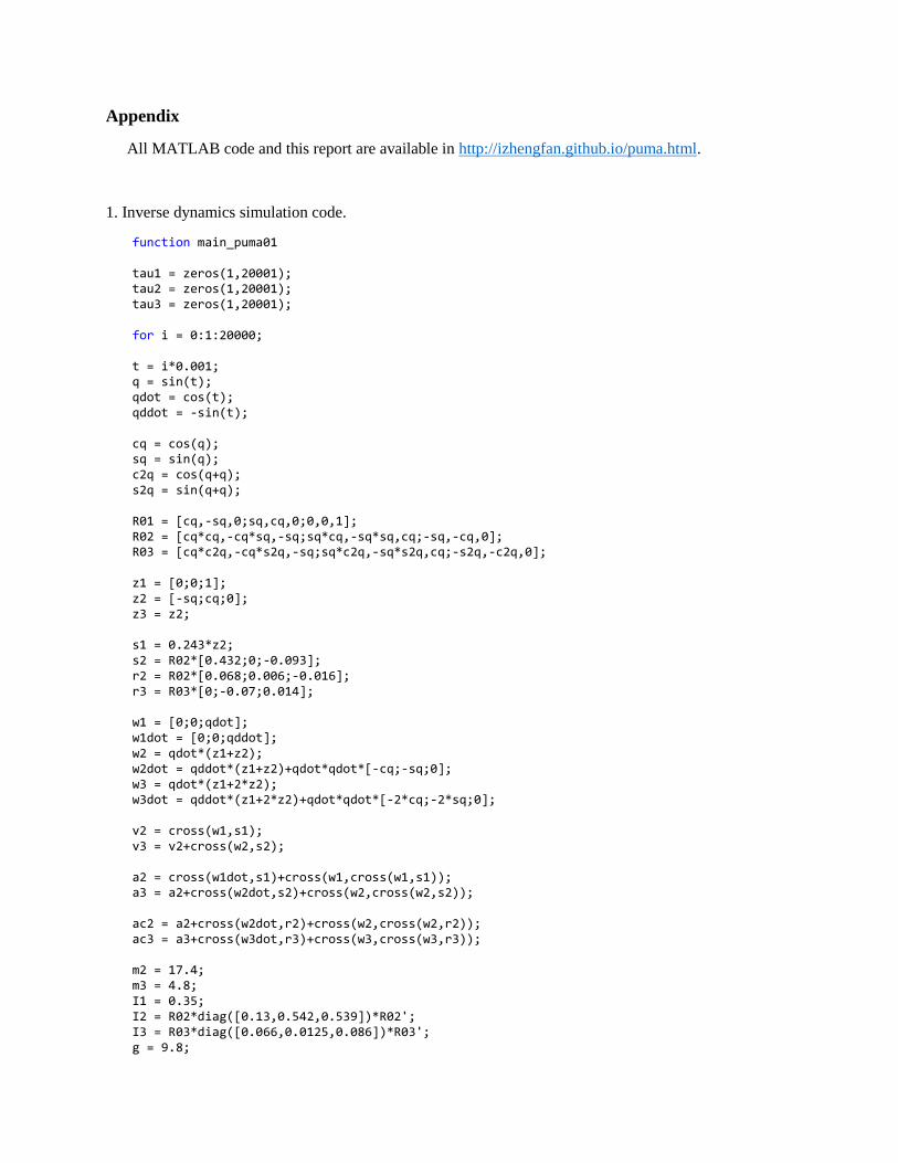
Appendix

All MATLAB code and this report are available in http://izhengfan.github.io/puma.html.

1. Inverse dynamics simulation code.

function main_puma01 tau1 = zeros(1,20001); tau2 = zeros(1,20001); tau3 = zeros(1,20001); for i = 0:1:20000; t = i*0.001; q = sin(t); qdot = cos(t); qddot = -sin(t); cq = cos(q); sq = sin(q); c2q = cos(q+q); s2q = sin(q+q); R01 = [cq,-sq,0;sq,cq,0;0,0,1]; R02 = [cq*cq,-cq*sq,-sq;sq*cq,-sq*sq,cq;-sq,-cq,0]; R03 = [cq*c2q,-cq*s2q,-sq;sq*c2q,-sq*s2q,cq;-s2q,-c2q,0]; z1 = [0;0;1]; z2 = [-sq;cq;0]; z3 = z2; s1 = 0.243*z2; s2 = R02*[0.432;0;-0.093]; r2 = R02*[0.068;0.006;-0.016]; r3 = R03*[0;-0.07;0.014]; w1 = [0;0;qdot]; w1dot = [0;0;qddot]; w2 = qdot*(z1+z2); w2dot = qddot*(z1+z2)+qdot*qdot*[-cq;-sq;0]; w3 = qdot*(z1+2*z2); w3dot = qddot*(z1+2*z2)+qdot*qdot*[-2*cq;-2*sq;0]; v2 = cross(w1,s1); v3 = v2+cross(w2,s2); a2 = cross(w1dot,s1)+cross(w1,cross(w1,s1)); a3 = a2+cross(w2dot,s2)+cross(w2,cross(w2,s2)); ac2 = a2+cross(w2dot,r2)+cross(w2,cross(w2,r2)); ac3 = a3+cross(w3dot,r3)+cross(w3,cross(w3,r3)); m2 = 17.4; m3 = 4.8; I1 = 0.35; I2 = R02*diag([0.13,0.542,0.539])*R02'; I3 = R03*diag([0.066,0.0125,0.086])*R03'; g = 9.8;

f3 = m3*ac3+[0;0;m3*g]; n3 = I3*w3dot+cross(w3,I3*w3)+cross(r3,f3); t3 = z3'*n3; f2 = m2*ac2+f3+[0;0;m2*g]; n2 = I2*w2dot+cross(w2,I2*w2)+cross(r2,f2)+n3+cross((s2-r2),f3); t2 = z2'*n2; n1 = I1*w1+n2+cross(s1,f2); t1 = z1'*n1; tau1(i+1) = t1; tau2(i+1) = t2; tau3(i+1) = t3; end t = 0:0.001:20; plot(t,tau1,'-',t,tau2,'--',t,tau3,'-.'); xlabel('t/s'),ylabel('\tau /Nm'); legend('\tau 1','\tau 2','\tau 3');

2. PD control simulation code

function main_puma_pd [t,x] = ode45(@puma_pd,0:0.001:20,[0 0 0 0 0 0]); plot(t,x(:,1),'-',t,x(:,2),'--',t,x(:,3),'-.','linewidth',2); legend('q1','q2','q3'); hold on plot(t,pi*ones(1,length(t))/2,'--'); xlabel('t/s'),ylabel('q/rad'); hold off end function xdot = puma_pd(~,q) xdot = zeros(6,1); qd = [pi/2; pi/2; pi/2]; A = [50 0 0; 0 180 0; 0 0 50]; B = [35 0 0; 0 50 0; 0 0 20]; tau = -A*([q(1);q(2);q(3)]-[qd(1);qd(2);qd(3)])-B*[q(4);q(5);q(6)]; xdot(1) = q(4); xdot(2) = q(5); xdot(3) = q(6); H = [22+0.9*cos(q(2))*cos(q(2)), 1.17+1.92*sin(q(2)), -0.3*cos(q(2)+q(3)); 1.17+1.92*sin(q(2)), 1.66, -0.29; -0.3*cos(q(2)+q(3)), -0.29, 0.11]; xdot(4:6) = H\(-... [-1.8*cos(q(2))*sin(q(2))*q(4)*q(5)+1.92*cos(q(2))*q(5)*q(5)+0.3*sin(q(2)+q(3))*(q(5)+q(6))*q(6); 91.9*sin(q(2))-3.3*sin(q(2)+q(3))+0.9*sin(q(2))*cos(q(2))*q(4)*q(4)-0.3*sin(q(2)+q(3))*q(4)*q(6); 0.3*sin(q(2)+q(3))*q(4)*q(5)-3.3*sin(q(2)+q(3))]+tau);

end

3. PID control simulation code

function main_puma_pid [t,x] = ode45(@puma_pid,0:0.001:20,[0 0 0 0 0 0 0 0 0]); plot(t,x(:,1),'-',t,x(:,2),'--',t,x(:,3),'-.','linewidth',2); legend('q1','q2','q3'); hold on plot(t,pi*ones(1,length(t))/2,'--'); xlabel('t/s'),ylabel('q/rad'); hold off end function xdot = puma_pid(~,q) xdot = zeros(9,1); qd = [pi/2; pi/2; pi/2]; A = [1200 0 0; 0 180 0; 0 0 50]; B = [300 0 0; 0 50 0; 0 0 10]; C = [300 0 0; 0 120 0; 0 0 10]; tau = -A*([q(1);q(2);q(3)]-[qd(1);qd(2);qd(3)])-B*[q(4);q(5);q(6)]-C*[q(7);q(8);q(9)]; xdot(1) = q(4); xdot(2) = q(5); xdot(3) = q(6); H = [22+0.9*cos(q(2))*cos(q(2)), 1.17+1.92*sin(q(2)), -0.3*cos(q(2)+q(3)); 1.17+1.92*sin(q(2)), 1.66, -0.29; -0.3*cos(q(2)+q(3)), -0.29, 0.11]; xdot(4:6) = H\(-... [-1.8*cos(q(2))*sin(q(2))*q(4)*q(5)+1.92*cos(q(2))*q(5)*q(5)+0.3*sin(q(2)+q(3))*(q(5)+q(6))*q(6); 91.9*sin(q(2))-3.3*sin(q(2)+q(3))+0.9*sin(q(2))*cos(q(2))*q(4)*q(4)-0.3*sin(q(2)+q(3))*q(4)*q(6); 0.3*sin(q(2)+q(3))*q(4)*q(5)-3.3*sin(q(2)+q(3))]+tau); xdot(7:9) = q(1:3)-qd; end

4. PD plus gravity compensation control simulation code

function main_puma_pdg [t,x] = ode45(@puma_pdg,0:0.001:20,[0 0 0 0 0 0]); plot(t,x(:,1),'-',t,x(:,2),'--',t,x(:,3),'-.','linewidth',2); legend('q1','q2','q3'); hold on plot(t,pi*ones(1,length(t))/2,'--'); xlabel('t/s'),ylabel('q/rad'); hold off end function xdot = puma_pdg(~,q) xdot = zeros(6,1); qd = [pi/2; pi/2; pi/2]; A = [500 0 0; 0 180 0; 0 0 50];

B = [350 0 0; 0 50 0; 0 0 20]; tau = -A*([q(1);q(2);q(3)]-[qd(1);qd(2);qd(3)])-B*[q(4);q(5);q(6)]; xdot(1) = q(4); xdot(2) = q(5); xdot(3) = q(6); H = [22+0.9*cos(q(2))*cos(q(2)), 1.17+1.92*sin(q(2)), -0.3*cos(q(2)+q(3)); 1.17+1.92*sin(q(2)), 1.66, -0.29; -0.3*cos(q(2)+q(3)), -0.29, 0.11]; xdot(4:6) = H\(-... [-1.8*cos(q(2))*sin(q(2))*q(4)*q(5)+1.92*cos(q(2))*q(5)*q(5)+0.3*sin(q(2)+q(3))*(q(5)+q(6))*q(6); 0.9*sin(q(2))*cos(q(2))*q(4)*q(4)-0.3*sin(q(2)+q(3))*q(4)*q(6); 0.3*sin(q(2)+q(3))*q(4)*q(5)]+tau); end

5. Computed torque control simulation code

function main_puma_ct [t,x] = ode45(@puma_ct,0:0.001:20,[0 0 0 0 0 0]); figure(1), plot(t,x(:,1),'-',t,x(:,2),'--',t,x(:,3),'-.','linewidth',2.5); legend('q1','q2','q3'); hold on plot(t,pi/2+sin(t),'--'); xlabel('t/s'),ylabel('q/rad'); hold off figure(2), plot(t,x(:,4),'-',t,x(:,5),'--',t,x(:,6),'-.','linewidth',2.5); legend('w1','w2','w3'); hold on plot(t,cos(t),'--'); xlabel('t/s'),ylabel('w/rad/s'); hold off end function xdot = puma_ct(t,q) xdot = zeros(6,1); qd = [pi/2+sin(t); pi/2+sin(t); pi/2+sin(t)]; qddot = [cos(t); cos(t); cos(t)]; qd2dot = -[sin(t); sin(t); sin(t)]; A = [500 0 0; 0 180 0; 0 0 50]; B = [350 0 0; 0 50 0; 0 0 20]; xdot(1) = q(4); xdot(2) = q(5); xdot(3) = q(6); xdot(4:6) = qd2dot - A*(q(4:6)-qddot) -B*(q(1:3)-qd); end