electrical distribution modeling: an integration of ... · friend, dr. jaime de la ree, has been...
TRANSCRIPT

Electrical Distribution Modeling:
An Integration of Engineering Analysis and Geographic Information Systems
by
Philip Hartley Smith
Thesis submitted to the Faculty of the
Virginia Polytechnic Institute and State University
in partial fulfillment of the requirements for the degree of
Master of Science
In
Electrical Engineering
APPROVED:
Jaime De La Ree, Chairman
Yilu Liu
Virgilio Centeno
December 15, 2005
Blacksburg, Virginia
Keywords: Geographic Information Systems, Power Distribution Systems, Modeling

Electrical Distribution Modeling: An Integration of Engineering Analysis and Geographic Information Systems
Philip Hartley Smith
Abstract
This thesis demonstrates the value of integrating electrical distribution engineering
analysis with Geographic Information Systems (GIS). The 37-Node IEEE Feeder model
was used as the base distribution system in this study. It was modeled separately, both in
software capable of unbalanced load-flow and in an industry-standard GIS environment.
Both tools utilized were commercially available, off-the shelf products indicative of those
used in academia and in basic GIS installations. The foundational data necessary to build
these models is representative of information required by a variety of utility departments for
a multitude of applications. It is inherent to most systems within an enterprise-level,
business-wide data model and therefore can be used to support a variety of applications. In
this instance, infrastructure information is assumed to be managed and housed with the GIS.
This data provides the required information as input for load-flow calculations. The
engineering analysis is performed within DistributionSystem 4.01 and its output is passed
back to the GIS in tabular format for incorporation. This thesis investigates the transfer of
information between GIS and DistributionSystem 4.01 and demonstrates the extended
display capabilities in the GIS environment. This research is implemented on a small scale,
but is intended to highlight the need for standardization and automatic integration of these
systems as well as others that are fundamental to the effective management of electrical
distribution systems.

Acknowledgments
I would like to express my deepest gratitude to my family and friends who have
supported me throughout this undertaking. First and foremost, I would like to thank my
wife and son, Lori and Levin for inspiring me through this entire challenge. My advisor and
friend, Dr. Jaime de la Ree, has been instrumental in nurturing my education both in
engineering and in spirit. I would also like to thank Bill Phillips and Kent Stover, of Wallops
Flight Facility, for their trust in me. I am extremely grateful for the cooperative educational
opportunity they have provided. It has allowed me the chance to uncover a deeply
interesting field of study, in power systems; to overcome one of the toughest challenges in
my life to date; to grow into the leadership role of project management; to work in a
motivating environment with a variety of assignments; and most importantly, the
opportunity will help me to raise my family on the Eastern Shore of Virginia. I will always
be in debt to my mother, father, and brother for their unwavering support of me in
everything I do.
iii

Table of Contents
Acknowledgments ............................................................................................................ iii Table of Contents ............................................................................................................. iv Acronyms ........................................................................................................................... v List of Figures................................................................................................................... vi List of Tables ................................................................................................................... vii Chapter 1 - Introduction.................................................................................................... 1
1.1 Overview of Geographic Information Systems ...................................................... 2 1.2 Purpose of Study ...................................................................................................... 4 1.3 Research Goals and Approach ................................................................................ 4
Chapter 2 – Literature Review .......................................................................................... 7 2.1 GIS Applications to Electric Utility Power Systems ............................................. 7 2.2 Engineering Analysis within GIS ........................................................................... 9 2.3 Existing Integration Solutions.............................................................................. 10 2.4 Distribution Management System Data Standards ............................................ 11
2.4.1 Common Information Model (CIM) ............................................................. 12 2.4.2 Other Data Models ......................................................................................... 13
Chapter 3 – Modeling 37-Node Network in DistributionSys 4.01 ............................... 15 3.1 DistributionSys....................................................................................................... 15 3.2 Modeling Methods ................................................................................................ 15 3.3 IEEE 37-Node Feeder Model .............................................................................. 17
3.3.1 Overview of IEEE Feeder Models................................................................. 18 3.3.2 Structure and Format...................................................................................... 19
3.4 Modeling IEEE 37-Node System Elements ....................................................... 20 3.4.1 Source............................................................................................................... 20 3.4.2 Nodes............................................................................................................... 21 3.4.3 Lines ................................................................................................................ 21 3.4.4 Loads ............................................................................................................... 23 3.4.5 Transformers ................................................................................................... 24
3.5 Load Flow Results ................................................................................................. 25 Chapter 4 – Modeling 37-Node Feeder in GIS.............................................................. 27
4.1 Spatial Graphics ..................................................................................................... 28 4.2 Attribution .............................................................................................................. 29 4.3 Building a Geodatabase ........................................................................................ 32 4.4 Building a Geometric Network ............................................................................ 33
Chapter 5 – Demonstration............................................................................................. 37 5.1 Engineering Results in the GIS Environment..................................................... 37 5.2 Building Engineering Model from GIS Data ...................................................... 44
Chapter 6 – Conclusions ................................................................................................. 48 Chapter 7 – Suggestions for Future Work ..................................................................... 49 References ........................................................................................................................ 51 Vita.................................................................................................................................... 53
iv

Acronyms
GIS Geographic Information System
CIM Common Information Model
ESRI Environmental Systems Research Institute
COTS Commercial, off-the-shelf
GPS Global Positioning Systems
IEC International Electrotechnical Commission
SIDM Systems Integration for Distribution Management
XML Extensible Markup Language
IEEE Institute of Electrical and Electronics Engineers
CAD Computer-Aided Design
SDSFIE Spatial Data Standard for Facilities, Infrastructure, and the Environment
FMSFIE Facilities Management Standard for Facilities, Infrastructure, and the
Environment
AM/FM Automated Mapping/ Facilities Management
EPRI Electric Power Research Institute
CCAPI Control Center Application Program Interface
DMS Distribution Management System
EMS Energy Management System
v

List of Figures
Figure 1. 1: Layering information in GIS (courtesy Miner & Miner) ........................................ 2 Figure 1. 2: The ESRI geodatabase architecture (courtesy ESRI)............................................ 3 Figure 1. 3: A schematic summary of the modeling process................................................. 6 Figure 2. 1: Damage Assessment Map (courtesy Dominion Power) ............................................. 9 Figure 3. 1 Graphical Modeling in DistributionSys ............................................................. 16 Figure 3. 2: Model-building template and Excel "worksheets" ............................................ 17 Figure 3. 3: Catalog of standard equipment. ....................................................................... 17 Figure 3. 4: IEEE 37 Node Test Feeder network schematic. .............................................. 18 Figure 3. 5: Underground Line Spacings............................................................................. 19 Figure 3. 6: Illustration of three-phase loads broken down and modeled per phase. ........... 25 Figure 4. 1: An overview of modeling the IEEE system in GIS.......................................... 28 Figure 4. 2: Joining attribution to shapefiles ....................................................................... 29 Figure 4. 3: GIS display of conductor type ......................................................................... 31 Figure 4. 4: GIS display of conductor ampacity .................................................................. 32 Figure 4. 5: IEEE 37-Node Geodatabase Structure ............................................................ 33 Figure 4. 6: Arrows indicating current flow direction and node/load identification. ........... 35 Figure 4. 7: Topological query (downstream trace) with open bus. ..................................... 36 Figure 5. 1: An example of conductor loading displayed within GIS................................... 39 Figure 5. 2: Calculation of accumulated Real Power loss from point to point. .................... 41 Figure 5. 3: Statistics on the real power losses from selected set. ........................................ 42 Figure 5. 4: Percent voltage drop at every bus. (Calculated from balanced load flow) ......... 43 Figure 5. 5: GIS field calculator used to create a new attribute column (% voltage drop).... 44 Figure 5. 6: Grids contain different geographic orientation................................................. 45 Figure 5. 7: Bitmap image of DistributionSys layout. .......................................................... 46 Figure 5. 8: Georeferencing verification results .................................................................. 47
vi

List of Tables
Table 3. 1: IEEE Feeder load models. ................................................................................ 19 Table 3. 2: IEEE 37-Node Regulator data .......................................................................... 20 Table 3. 3: Excerpt of line attributes output from DistributionSys...................................... 22 Table 3. 4: Summary of cable configurations used in model................................................ 22 Table 3. 5: Comparison of cable reactance estimates. ......................................................... 23 Table 4. 1: Summary of shapefiles and supporting datasets................................................. 27
vii

Chapter 1 - Introduction
Traditionally, power systems analysis has been performed within software that is
specifically tailored to the needs of an engineer. These tools are highly successful and
satisfactory for the calculation of load flow, protection settings, short circuit analysis,
harmonic analysis, etc. In addition, it is important to recognize that the information required
to perform these calculations is also utilized in other forms of system management. For
example, to establish protective device settings for a distribution feeder, an engineer needs to
know attributes such as cable length, configuration, material, and size. Likewise, a power
system manager, involved in planning for expansion, needs to know the very same
information on the feeder to determine the available capacity for growth. In large part, this
is a database function and can be served from a business-wide information system [1].
To take this notion one step further than a traditional relational database, the idea of
locational or spatial information can be incorporated. No information system handles this
better than a Geographical Information System (GIS). Organizing information in a GIS
satisfies the need for data storage and accessibility just like other information systems.
However, GIS is built from a mapping foundation and thus creates a visual interface to the
data. In addition to normal database queries, information can be examined through a variety
of spatial attributes such as distance, proximity, and elevation (to name a few).
Another function that sets GIS apart from simple columns and rows is its ability to
integrate information from a variety of sources. For example, a traditional power system
database could answer many specific questions on an electrical distribution system.
However, it may not be able to address the system’s interaction with its surroundings. For
instance, in planning the installation of a distributed generator there are certain
environmental, social, and infrastructure-related criteria needed to fully assess the situation
[2]. In a GIS environment, these factors would be virtual layers of information that are
“draped” over the existing electrical system as in Figure 1.1. There is no better way to
visualize this scenario than within the mapping environment. This thesis illustrates the
extended capabilities that GIS provides to traditional power system engineering analysis
techniques.
1

Figure 1. 1: Layering information in GIS (courtesy Miner & Miner)
1.1 Overview of Geographic Information Systems
Geographic Information Systems come in all shapes and sizes. Some are project-
specific and support a single initiative for a fixed period of time. They may be primarily
utilized for presentation purposes due to their spatial analysis or cartographic capabilities.
Other, more dynamic systems have the capability of relating vast amounts of information
through database functionality, as well as spatial analyses. These systems are often built
around data that may be created and maintained by different people in various
environments. With proper coordination and database design, all information (including
database, imagery, video, spatial, etc.) can be linked through map graphics that ultimately tie
back to a location on the earth’s surface. Essentially, regardless of scale, a GIS is a container
of information that can be extracted through a map view. The old adage, “a picture is worth
a thousand words,” is a simple description of the effectiveness of GIS in communicating or
expressing complicated information in a highly intuitive manner.
Environmental Systems Research Institute (ESRI), the world leader in Geographic
Information Systems’ technology, defines a GIS as “an arrangement of computer hardware,
2

software, and geographic data that people interact with to integrate, analyze, and visualize data; identify
relationships, patterns, and trends; and find solutions to problems. The system is designed to capture, store,
update, manipulate, analyze, and display the geographic information. A GIS is typically used to represent
maps as data layers that can be studied and used to perform analyses.”
ESRI offers a suite of scalable GIS tools that can be utilized in virtually any
application. ESRI’s tools address desktop analysis, mobile needs, web delivery,
programming/development, and a variety of customized extensions. The integration of
various data sources and the structure necessary to manage these types of systems is handled
in GIS by a data model called the geodatabase. Its basic structure and components of this
“geographic” database can be seen in Figure 1.2. This research focuses on a geodatabase
solution and it highlights the ability of GIS to integrate data that is traditionally maintained in
a different environment. Also, this work illustrates the added capabilities achieved through
modeling an electrical distribution system in GIS.
Figure 1. 2: The ESRI geodatabase architecture (courtesy ESRI)
3

1.2 Purpose of Study
It is the intent of this study to explore the data exchange between a Geographic
Information System and a power system analysis toolset. In today’s day and age, most
facility infrastructure information is maintained in some form of database or information
system. In many cases, these attributes are stored in a central data repository capable of
managing an enterprise type system, which is defined by ESRI as a system that “supports
strategic business decisions or large databases across multiple departments in an organization.” One such
arrangement, referred to as a Geographic Information System, provides a robust relational
data structure, coupled with a spatial (mapping) component. These systems are often used
to manage and share information across disciplines or between departments through a map
interface.
This thesis documents a specific application of GIS to common power system
engineering practices, whereby information inherent to a GIS model provides the necessary
input data to run a load-flow analysis within an external engineering software package. As
indicated by L.V. Trussel, there are four reasons why GIS is a capable source of data to feed
engineering analysis in many utilities [3]:
1) GIS is commercially available in industry standard software (like AutoCAD®);
2) GIS can manage a broad swath of information across department lines;
3) The use of XML and open source database technologies enables sharing;
4) Reporting can be accomplished through standard web-interfaces.
In addition to feeding the load-flow model, the engineering results will be returned
into the spatial (graphical) mapping display within the GIS. This exercise will showcase the
interoperability of GIS and highlight the flexibility it possesses to extend into the technical
realm of engineering.
1.3 Research Goals and Approach
This thesis presents the application of Geographic Information Systems to the
engineering of electrical distribution systems. Currently, customized solutions exist for this
integration. There are engineering software packages capable of utilizing GIS display
4

capabilities and conversely, there are customized GIS extensions aimed at capturing
engineering toolsets. However, this research presents an integration solution using basic
GIS software that is readily available and currently in place at most businesses and
universities. Under this premise, the objective of this research includes the following goals:
1. To extend spatial analysis and display capabilities into traditional Power
System studies,
2. To apply basic Commercial, Off-the-Shelf (COTS) GIS products to power
system analysis,
3. To demonstrate that an existing GIS can provide the necessary data to run
load flow analysis,
4. To display and query load flow results in a mapping environment, and
5. To investigate the transfer of information between GIS and an engineering
software-package (DistributionSys, Version 4.01).
To achieve these goals, six steps were applied. To start, a geodatabase was
constructed to model the IEEE 37-Bus distribution feeder in GIS. From the perspective of
an engineer, this model could represent an existing data source, possibly maintained in
another branch or office of a business. Next, utilizing this GIS model of an electrical
distribution system, data was exported into a format that was compatible with
DistributionSys engineering software. Thirdly, load flow analysis was performed within the
engineering application. As a follow-on step, the results were incorporated back into the
existing geodatabase in the GIS environment. In the fifth stage, the engineering analysis
results were queried within GIS, to demonstrate the added capabilities delivered through the
integration. As a final step, to demonstrate the passing of information from GIS back to
DistributionSys, the engineering model was automatically generated from existing GIS
tabular information. The entire information exchange is summarized in Figure 1.3.
5

Figure 1. 3: A schematic summary of the modeling process
6

Chapter 2 – Literature Review
2.1 GIS Applications to Electric Utility Power Systems
To obtain a full understanding of the broad capabilities that Geographic Information
Systems bring to the realm of electric utility management, it is necessary to recognize some
existing applications throughout the industry. GIS systems in large companies often bridge
the gap between many different information systems and by their mere existence, provide
basic management tools. The following list highlights a variety of specific GIS applications
within different electric utilities. It is important to recognize that most, if not all of these
applications offer a variety of financial, business, engineering, and construction planning
tools inherent to an enterprise GIS solution.
Vegetation Management: To highlight the importance of vegetation management, it is
necessary to point out that after the major blackout in August 2003, a bi-national task force
(U.S. and Canada) determined that a major factor contributing to the blackout was tree
contact with transmission lines. The New York Power Authority (NYPA) has an exemplary
vegetation management program in place to protect its 1,400 circuit miles of high voltage
transmission lines. This system is an enterprise GIS that ties together information from land
management, equipment maintenance, environmental, and engineering disciplines. This tool
was developed to help NYPA manage the company’s 16,000 acres of high voltage right-of-
way. In the past, NYPA utilized “as-built” construction drawings to delineate the vegetation
profiles for right-of-ways. The use of static design drawings to document ever-changing
vegetation was difficult to keep current. GIS, coupled with GPS surveying technologies, has
allowed NYPA to integrate spatial mapping into the planning of right-of-way maintenance
and treatments. It has also allowed managers to compare the effectiveness of treatments
from one year to the next. The ability to monitor the effectiveness of treatments has helped
NYPA minimize herbicide applications, both saving money and mitigating ecological affects
[4].
Land Management: American Electric Power (AEP) utilizes GIS to manage its own
300,000 acres of real estate property. Since its incorporation in 1906, AEP has managed its
land transfer records on paper, organized in file cabinets. This system has been made more
7

efficient by organizing these records and new transactions into an enterprise GIS. Property
boundaries are now maintained in a digital format and are no longer hand-drawn. Extensive
field surveys are no longer needed to close a sale on land since the property boundaries are
readily available and accurate. This function is highly valuable because in the past, the profit
made on land transfers was often offset by the cost in time and money of surveying their
own property boundaries. This application of GIS technology helps distribute important
real property information to the company’s real estate agents, legal, and other personnel via
the AEP intranet [5].
Emergency Management: Dominion Electric’s GIS provided important disaster
management support in September 2003, during Hurricane Isabel. During that storm, more
than 1.8 million customers (out of 2.2 million, total) in Virginia and North Carolina lost
electrical power. Dominion’s enterprise GIS provided support during the hurricane by
tracking damages, analyzing outages, prioritizing work orders, and organizing logistics for the
recovery effort. This GIS system had been built in previous years to support outage
management, feeder connectivity, engineering plat production, and overall asset
management. Its role in restoring power to Dominion’s customers increased down time by
streamlining the response to this disaster. In addition, Dominion provides a web-based GIS
service delineating current outages in the company’s service area. This tool was used
650,000 times during the two-week Isabel recovery and is an example of how utilities are
using GIS technology to disseminate important information [6].
8

Figure 2. 1: Damage Assessment Map (courtesy Dominion Power)
Environmental Management: The Companhia Paranaense de Energia (COPEL) in
Brazil utilizes GIS as a planning tool to address its interaction with the local environment.
The Brazilian state of Parana maintains environmental regulations enacted to protect
forested areas, to prevent erosion, to maintain agrarian fertility, and to mitigate pollution.
COPEL adopted an environmental management tool that utilizes GIS to help manage the
company’s environmental compliance.
COPEL is a large electric utility that owns 18 power plants, 17 of which are
hydroelectric. The utility’s decision makers utilize this system to weigh the costs versus
benefits when faced with planning the location of new hydroelectric facilities. COPEL’s
environmental GIS allows the utility to consider demographics, health, and environmental
effects when planning for expansion or growth. In addition, this system allows dam water
management and provides for the relocation plans necessary during the construction of a
new hydroelectric power plant. This system was tested recently during the construction of a
new hydroelectric facility where it created the contingency plans for damage to the dam [7].
2.2 Engineering Analysis within GIS
In the current state of the industry, electric utilities are faced with ever-increasing
competition. They are required to produce more power, at higher reliability, with fewer
planning staff. Oftentimes, GIS is a system that enables greater corporate efficiency through
9
the effective sharing and distribution of information. Utilities that have mature data
processes and good corporate information systems can compete more effectively in today’s
market. Furthermore, those businesses that have sound information systems can leverage
existing data to support engineering analysis (as well as other specific applications). Utilizing
existing corporate information is the logical choice to avoid redundancy and synchronization
issues. Therefore, in utility environments that have existing GIS, it makes good business
sense to integrate engineering analysis within the envelope of the corporate information
system structure.
Within a utility’s corporate information system, engineering applications demand the
highest quality, and the most specific datasets. In addition to utilizing information that is
common to the business model, engineering analysis also requires data that may not
normally reside within the GIS. As indicated by Trussell and Kenney, any integration of GIS
and engineering analysis will require implementation of network tracing, data conversion,
validation, additional engineering parameters, and software execution [8].
There are a variety of ways to integrate GIS and engineering analysis. The most basic
technique, data extraction, will be utilized in this research. Extraction refers to drawing
information from the GIS, supplementing it with the data required by engineering analysis,
and exporting it to its own database. This approach provides the engineer with total control
of the information, but presents maintenance problems because any changes made by the
engineer aren’t incorporated back into the enterprise data system [8]. It is important to
recognize, though it is beyond the scope of this work, that a variety of integration scenarios
exist to automate this process on an enterprise level. Some of these integrations are
packaged in proprietary software solutions and will be summarized in the following section.
2.3 Existing Integration Solutions
The goal of integrating GIS and engineering analysis is to create technically valid
reporting capabilities within the GIS environment. As indicated in the previous section,
there are a variety of integration solutions available that are scalable to specific needs.
From a GIS vantage point, there exist commercially-available, custom solutions for
integrating engineering capabilities through ESRI partners. For example, Miner & Miner
offers ArcFM®, a powerful extension to basic GIS. This extension is an enterprise solution
tailored to the needs of utility system management. Engineering capability exists within the
10

extension to interface the infrastructure model with “third-party” engineering analysis
engines. The “Network Adapter” to ArcFM® allows an engineering model to be extracted
from the existing GIS data and loaded via XML into the analysis engine. Also, it allows for
the flow of information back into the GIS, in the opposite direction. In essence, this tool
provides an interface between the GIS and the engineering analysis software package. The
model templates are structured to work with ESRI’s Electrical Distribution data model and
interface with common analysis packages such as CYME's CYMDIST®, Advantica Stoner's
Electric Solver®, and Milsoft’s Windmil® (used for load flow on IEEE test feeders [9]).
From a power systems analysis perspective, there also exist solutions designed by the
software vendors to integrate their engineering analysis tools with GIS. For example,
Siemens Corporation offers engines to extend the traditional power systems analysis
capabilities of PSS/E® into the realm of GIS. PSS/Engines® contain the algorithms
necessary to perform different analyses of electrical distribution networks. These engines
can be called from virtually any programming language, including Visual Basic, the common
language of the current ESRI ArcGIS® platform.
There are many examples of customized integration solutions on the market today.
However, the scope of this research will focus on a non-proprietary, basic GIS integration
using tools that are readily available at most businesses or universities.
2.4 Distribution Management System Data Standards
With the onset of deregulation and under heightened competition, utilities are facing
great challenges in the exchange of distribution system information. Energy management
systems (EMS) are often employed to model transmission systems and have matured greatly
to support such critical infrastructure. However, the demands of distribution management
are quite different and require more information for a variety of reasons. Primarily,
distribution systems have very large information models, and as a result, require tracking and
accounting for many more system components. Distribution systems data models are also
larger in size, having on the order of 500,000 to 10,000,000 objects [10].
Adding to the complexity, there are many different system interactions. For
example, a distribution management system (DMS) needs to incorporate a customer
information system, a geographic information system, an outage management system, a
11
maintenance tracking system, as well as many more applications to effectively manage the
delivery of electricity to its customers.
In addition to the amount of information and the broad variety needed, system
changes occur more frequently in distribution systems when compared to transmission
networks. There are constant maintenance changes that need to be tracked as well as
operational/control modifications in distribution systems. The DMS needs to be flexible to
reflect the ever-changing conditions inherent to an electrical distribution system.
The magnitude and complexity of the data required to manage a distribution system
warrants its own standard. As is with most Distribution Management Systems, the sub-
systems and their respective datasets often reside in proprietary software packages. This
presents a problem in the effective exchange of information across departments. To design
and implement a streamlined enterprise information system for utility system management,
there needs to be standard data model for distribution networks. This standard provides a
target for software development and interoperability. It also integrates both engineering and
business functions. The Common Information Model (CIM) is currently being applied to
distribution systems and standardized through the International Electrotechnical
Commission (IEC) [10], [11].
2.4.1 Common Information Model (CIM)
The Common Information Model was originally developed by the Electric Power
Research Institute (EPRI) as a framework for an integration called the Control Center
Application Program Interface (CCAPI) [10], [11] [1]. This model was constructed to
integrate the control center environment with business functions by facilitating the
information exchange between different computer systems and applications. The Common
Information Model (CIM) was a large part of this standard and was originally representative
of information inherent to transmission networks. As the need for a modified distribution
system data model became more evident, the IEC Technical Committee 57 Working Group
14 took on the task of standardizing an information model for “Systems Integration for
Distribution Management (SIDM).” The prefacing work to standardize the CIM for energy
management systems resides under the purview of Working Group 13. Websites dedicated
to these working groups are available at the following locations:
12

IEC TC57 WG14: http://www.wg14.com/
IEC TC57 WG13: http://www.wg13.com/
The CIM is a logical data model that provides a framework and theory for the
various relationships of distribution system information. The actual physical
implementations of this model are vendor specific and may vary. In addition to developing
a standard model, it is very important to develop the physical tools that coordinate data for
import and export in accordance with the CIM. Xiaofeng Wang has proposed modifications
to the existing CIM to extend the model into distribution realm for load flow capabilities.
This work takes the IEEE Feeder Models [9] developed by Professor Kersting and adapts
them to the CIM as extensible markup language (XML) documents. Though Geographic
Information Systems are considered by the IEC as sub-systems within the CIM, many of the
modeling issues identified by Wang parallel those experienced through this research. The
modeling in this project was not in accordance with the CIM, but the techniques and the
data model indicated in Wang’s work were referred to throughout the entire process. Wang
modeled the IEEE Feeders in XML and it is the intent of this work to do the same in a
graphical manner through the GIS [10].
2.4.2 Other Data Models
It is important to recognize the existence of multiple standards for the modeling of
electrical distribution systems. The aforementioned data model is a product of the IEC and
is geared toward the international implementation for electrical utilities. The CIM structure
encompasses both technical and business functions into one enterprise level information
system typical for utilities. This model addresses the management of immense amounts of
information and views GIS as an Automated Mapping/Facilities Management tool.
In addition, ESRI maintains an electrical distribution system data model to support
engineering, construction, and operational needs. This model focuses primarily on
infrastructure management. It is tailored to the needs of management, operations, and
maintenance of the infrastructure life-cycle to help maintain current as-built information. It
intends to integrate computer-aided design (CAD) drawings with the GIS network as well as
providing integration capabilities with other systems responsible for managing outages,
documents, materials, customer information, et cetera [12] [1].
13

Another standard data model available for system representation is the Spatial Data
Standard for Facilities, Infrastructure, and the Environment (SDSFIE). This logical data
model was developed through a cooperative effort between the three U.S. Department of
Defense military services (Army, Air Force, and the Navy). Its original intent was to provide
a standardized model for federal facilities management information. It evolved to include a
broader vision of dissemination beyond the Department of Defense and federal facilities.
The Facilities Management Standard for Facilities, Infrastructure, and the Environment
(FMSFIE) portion addresses the management of enterprise level information that relates to
the infrastructure data. The SDSFIE is a spatial data model and primarily addresses features
that have been mapped in either the CAD or GIS environment. This model is tied to the
FMSFIE through valuable relationships inherent to virtually any organization charged with
the management of facilities. These standards offer more than theoretical data models. The
strength of this format lies in the availability of non-proprietary tools. This standard offers
free tools for the construction of empty GIS data as well as the construction of a “skeleton”
relational database structure. The published tools are updated frequently and provide the
import/export toolset imperative to the success of a large implementation [13], [14], [15].
The work documented in this thesis does not adhere to any one standard, though it
pulls logical modeling techniques from the standards referenced above. It is beyond the
scope of this work to compare the pros and cons of these modeling approaches. However,
further work could be undertaken to investigate the differences.
14

Chapter 3 – Modeling 37-Node Network in DistributionSys 4.01
3.1 DistributionSys
DistributionSys 4.01 is an
electrical distribution analysis software
package developed by Dr. Alexis Martínez
del Sol of the University of Guadalajara,
Mexico. This software allows for the
modeling of distribution system
components and provides the analysis
tools necessary to perform standard engineering calculations such as load flow, bus voltage,
transformer loadability, and protection analysis.
Network models can be built within DistributionSys from a schematic view or from
existing attribute data. The software is capable of importing and exporting information from
Microsoft Excel, making it a good candidate for GIS integration. In addition, the object-
oriented model can be built from a customizable catalog of system component information.
DistributionSys is capable of calculating balanced and unbalanced load-flow. This
analysis produces both detailed and summarized accounts of system losses, line flows, and
voltage at every node or bus. The software is capable of recommending optimum capacitor
placement, wire size upgrades, and changes in conductor configuration to satisfy user-
defined restrictions on the system. DistributionSys contains a tool to calculate maximum
and minimum short-circuit current at system nodes as well as the ability to analyze
protection settings. The software can check the coordination of settings against a given
scenario and identify uncoordinated devices.
Once a system is modeled correctly in DistributionSys, the analysis tools available
enable a wealth of capability. Since the output results from these analyses can be exported to
Excel, they can be displayed in a GIS environment to further extend the reporting
capabilities. Conversely, since the system models can be built from an Excel template, an
existing GIS model (if formatted correctly) could provide all of the information necessary to
automatically build a network model in DistributionSys [16].
3.2 Modeling Methods
15

System models can be created through a graphical-user-interface or by importing
system information from a spreadsheet. If designed graphically, the system is drawn node-
by-node or line-by-line. The specific parameters can be entered for each component and
can be either selected from a standard catalog of equipment or customized to fit the
particular system component. The following screenshot demonstrates the graphical
modeling option:
Figure 3. 1 Graphical Modeling in DistributionSys
Electrical distribution system models can also be developed automatically within
DistributionSys by importing system information through the standardized Microsoft Excel
template (provided as an ancillary file with full installation). This template provides the
spreadsheet structure that the software can recognize. Once the correct cells and worksheets
are populated with system information, the template can be imported into DistributionSys
and a model can be automatically generated. The template is an Excel file of extension
“.xls” and is formatted such that each feature (i.e. line, load, bus, transformer, etc.) has its
own spreadsheet on a separate “worksheet”. “Worksheets” are delineated as tabs across the
bottom of an Excel spreadsheet. The following figure is an example:
16

Figure 3. 2: Model-building template and Excel "worksheets"
The modeling procedure within DistributionSys is greatly simplified by the existence
of its “Standard Catalog.” This is a database of common system information that includes
cable configurations, transformer connections, equipment ratings, voltage levels, and other
standard attributes. This feature allows a user to select equipment that already has defined
electrical parameters. For example, when modeling overhead powerlines, a user may select
from dropdown menus, a set of aerial, three-phase, ACSR 477 conductors with a certain
pole-top spacing configuration. Using this information and the length of the line,
DistributionSys estimates the impedance by calculating the line’s phase impedance matrix.
The information contained within the Standard Catalog greatly simplifies the modeling
procedure. In addition, the catalog can be modified to add unique components or to change
the characteristics of existing attributes. The “Standard Catalog” can be seen in Figure 3.3.
Figure 3. 3: Catalog of standard equipment.
3.3 IEEE 37-Node Feeder Model
17

3.3.1 Overview of IEEE Feeder Models
In 1992, the IEEE Distribution Analysis Subcommittee published a report providing
five benchmark electrical distribution system models. These models were developed to
provide a common set of system information for software developers to test and verify the
accuracy of engineering solutions. Detailed equipment information is included in the report
as well as the solutions to various power system analyses. All solutions were performed
using the Radial Distribution Analysis Package from WH Power Consultants and/or
Windmil® developed by Milsoft Integrated Solutions [9].
The 37 Node Test Feeder model was selected as the system of choice for this
research. It represents an actual underground radial distribution feeder in California
operating at 4.8kV under heavy phase imbalances. The schematic view of this network can
be seen in the following figure:
Figure 3.4: IEEE 37 Node Test Feeder network schematic.
18

All loads on this system are modeled as “spot” loads (some other IEEE models
contain continuous, or distributed loads). Table 3.1 contains the various types of load
models found in the IEEE radial distribution feeder systems.
Table 3. 1: IEEE Feeder load models.
Loads are delineated as delta or wye connection and as constant power, impedance,
or current. Constant impedance and current loads are determined by assuming a system
voltage of 1 per unit. The 37-Node Feeder is configured as a three-wire delta system and
therefore has no wye connected loads. It does, however, have many different line-to-line
loads that contribute to unbalanced conditions.
All conductors in the 37-Node model are assumed to be of the three-wire, delta
configuration. In addition, they are buried underground with a Spacing ID of 515,
corresponding to configuration in the following figure:
Figure 3. 5: Underground Line Spacings
Conductor line segment data contains “from” and “to” nodes as well as the actual
cable length per phase between nodes. The total result of this data plus individual conductor
sizes provides for the calculation of phase impedance and admittance matrices, a
fundamental part of distribution system analyses.
3.3.2 Structure and Format
19

For the purposes of this research, the GIS model is built from existing tabular data
provided by the IEEE 37 Node Feeder model. The data is available from the report in the
form of excel spreadsheets and can be found at the following IEEE URL:
http://ewh.ieee.org/soc/pes/dsacom/testfeeders.html
The tabular datasets provide all of the information necessary to perform standard
power system analyses such as load flow, bus voltage, and line current calculations. It is
important to recognize that when maintained within GIS, this model isn’t limited to
engineering analysis. The GIS model of the distribution system can easily integrate other
data sources to allow applications such as those mentioned previously in Section 2
(operations and maintenance, outage response, environmental, dig permitting, etc) [15].
3.4 Modeling IEEE 37-Node System Elements
3.4.1 Source
The IEEE 37-Node system was modeled in DistributionSys to enable its analysis and
reporting capabilities. The system of interest, as introduced in Section 3.3.1, was a 4.8kV
network configured delta and distributed underground in a three-wire configuration. The
IEEE system source is designated as two single-phase regulators, configured as open delta.
The following table summarizes the regulator information.
Regulator Data Regulator ID: 1
Line Segment: 799 -701
Location: 799
Phases: A - B -C
Connection: AB - CB
Monitoring Phase: AB & CB
Bandwidth: 2.0 volts
PT Ratio: 40
Primary CT Rating: 350
Compensator Settings: Ph-AB Ph-CB
R - Setting: 1.5 1.5
X - Setting: 3 3
Voltage Level: 122 122
Table 3. 2: IEEE 37-Node Regulator data
For the purposes of this research, the regulator was modeled in DistributionSys as a
substation consisting of a lossless, three-phase transformer (4.8kV/4.8kV) connected to a
20

source of infinite short-circuit current. The lossless transformer’s kVA rating and the
available fault current were set unrealistically high to act as infinite.
3.4.2 Nodes
All 37 nodes from the IEEE system were modeled in DistributionSys as primary
nodes. As they were drawn in graphically, the software assigned coordinate information to
the nodes based on their location in the Cartesian grid. This feature is important to
recognize since the idea of locational coordinates is inherent to a GIS model. When drawn
in DistributionSys, the network busses are assigned Cartesian coordinates (Figure 3.6) and
the resulting product is an unscaled network schematic. When the model is built in GIS, the
coordinates are referenced to the earth’s surface and act to scale the entire network so
distance and direction between nodes becomes meaningful.
Figure 3. 6: DistributionSys Cartesian coordinates assigned to nodes.
3.4.3 Lines
Conductors were modeled as they had been in the IEEE to be separate line
segments between nodes. To simplify the transition to GIS, the conductors were given a
name based on the upstream and downstream nodes. The format follows the convention of
combining the names of “from node” with “to node” into one, unique, six-digit code for
every line. Since the system is entirely radial, this naming convention works for every line in
the system and will provide the bridge between DistributionSys and GIS for displaying line
losses, and line power flows. Table 3.3 displays a tabular snapshot of line attributes exported
from DistributionSys into Excel.
21

Name From Node
To Node
Length (m) Phases
Conductor Configuration
R (ohm)
X (ohm)
R0 (ohm)
X0 (ohm)
799701 799 701 564 Trifásica Configuration 721 0.012 0.04 0.06 0.2 701702 701 702 293 Trifásica Configuration 722 0.013 0.023 0.06 0.12 702713 702 713 110 Trifásica Configuration 723 0.018 0.011 0.08 0.05 702703 702 703 402 Trifásica Configuration 722 0.017 0.032 0.08 0.16 702705 702 705 122 Trifásica Configuration 724 0.039 0.013 0.18 0.07 705712 705 712 73 Trifásica Configuration 724 0.023 0.008 0.1 0.04 705742 705 742 97 Trifásica Configuration 724 0.031 0.01 0.14 0.05 713704 713 704 159 Trifásica Configuration 723 0.025 0.016 0.11 0.08 704720 704 720 244 Trifásica Configuration 723 0.039 0.024 0.17 0.12
Table 3. 3: Excerpt of line attributes output from DistributionSys.
All lines were modeled as three-wire delta, no neutral. The configurations were
assigned based on those given in the IEEE 37-Node model. The four different cable
configurations were entered into the DistributionSys “standard catalog.” Since they were
added to the database, their electrical parameters were also estimated and logged.
Config. Conductor Type R
(ohms/mile) Dia. (in)
GMR (feet) microS/mile
Rating (A)
R (microhms/m)
X (microhms/m) C (pF/m)
721 1,000,000
CM AA 0.105 1.15 0.0368 159.7919 698 65.244 214.034 263.509 722 500,000 CM AA 0.206 0.813 0.026 127.8306 483 128.002 240.215 210.802 723 #2/0 AA 0.769 0.414 0.0125 74.8405 230 477.834 295.406 123.418 724 #2 AA 1.54 0.292 0.00883 60.2483 156 956.912 321.599 99.354
Table 3. 4: Summary of cable configurations used in model.
In table 3.4, columns “Config.”, “Conductor”, “Type”, “R(ohms/mile)”,
“Diam.(in)”, “GMR(feet)”, and “Rating (A)” were all provided by the IEEE excel tables.
“Microsiemens per mile” were taken from the estimated admittance matrices generated by
Milsoft software. This value corresponds to the capacitive admittance observed in
underground conductors. In DistributionSys, the parameter used to estimate the capacitive
reactance in underground conductor configurations is picofarads per meter. Therefore,
column “C (pF/m)” is simply the capacitance per unit length converted from the admittance
at 60 hertz using the following equation:
⎥⎦
⎤⎢⎣
⎡⋅
⋅⋅⋅⋅=
FpF
SF
SS
mmile
mileS
mpF 12
6
10)602(101609 πµ
µ
22

Inductive reactance per unit length was calculated using conductor spacing information (per
Figure 3.5) and the Geometric Mean Radius (GMR) from the table above. The equation is
as follows [17]:
[ ]⎥⎥⎥⎥
⎦
⎤
⎢⎢⎢⎢
⎣
⎡
⋅
⋅⋅⋅⋅⋅⋅=
Ω −
ftftGMRm "12)(
"12"6"6ln1026023
7πµ
As a check, the calculated reactance values were on the same order of magnitude as
those given by DistributionSys for similar (but not exact) conductor types and
configurations. DistributionSys contains values for underground 1000MCM, 500MCM, 2/0,
and #2 XLP three-phase conductors of unknown spacing. The comparison is summarized
in the following table:
General Underground Cable Type Calculated microhms/m Pre-Determined microhms/m
1000 MCM AA 214.03 237.70 500 MCM AA 240.21 266.00
2/0 AA 295.41 318.10 #2 AA 321.60 347.00
Table 3. 5: Comparison of cable reactance estimates.
Calculated values were used to create new conductor configurations within the
Standard Catalog of DistributionSys. Their comparison serves as a check against the validity
of the model to ensure practical results but does not intend to match exactly with the IEEE
feeder model. The goal of this research is to utilize GIS for display and to demonstrate the
enhanced capabilities that GIS provides. Testing with the IEEE model to exactly match
results is not the intent of this undertaking.
3.4.4 Loads
All loads from the IEEE 37-Node Feeder system were modeled as either constant
current, constant impedance, or constant power loads. These demand types were entered
into the Standard Catalog of DistributionSys under load profiles. Since the software allows
for varying loads over the course of the day, the IEEE loads were modeled as continuous
and delineated as either constant current, constant impedance, or constant power (See Figure
3.7)
23

Figure 3. 7: Load Modeling in DistributionSys.
3.4.5 Transformers
Modeling transformers in DistributionSys in accomplished in the representation of
loads. When a load is added to a particular bus, the user is prompted to choose the type of
transformer and its particular connection. In addition, when modeling primary loads within
the software, the user also identifies the type of load (from above; Section 3.4.4). For this
research, all the transformers and loads were entered in advance into the Standard Catalog to
simplify the modeling process. Transformers were modeled as lossless, 4.8kV/4.8kV delta
connections. All loads (though three-phase) were modeled as single-phase transformers and
loads. Breaking the loads up by phase simplified the modeling process since the IEEE
network was created to simulate heavy phase imbalances. For example, this idea is illustrated
in Figure 3.6 where the three-phase, constant-PQ load attached to bus 701 is split into three
separate loads. Each load is attached through a lossless, 4.8kV/4.8kV delta transformer and
has a continuous demand at rated load. Each load is designated to be connected across its
respective phases and as a result, it is applied as intended by the IEEE model.
24

Figure 3. 6: Illustration of three-phase loads broken down and modeled per phase.
3.5 Load Flow Results
Load flow results from DistributionSys can be exported in tabular format. For
unbalanced load flow, line current and phase angle is given for all three phases. Total real
power losses and kilowatt-hour losses are given per line but are lumped into one total
measurement that is combined for all three phases. Reactive power flow and losses aren’t
given, but can easily be calculated from the output information. For balanced flow, results
are similar, but as expected, line currents and angles are lumped into one, single-line
measurement.
The format of the output is manageable with some minor adjustments. For example,
bus voltage, line losses, and summary calculations are placed on the same excel worksheet
even though they don’t have the same column/row structure. Therefore, to make use of
this information, it must be manually regrouped by “cutting and pasting” the individual
datasets to separate files. For this research, the effort is minimal. However, for a large
power system with many nodes and multitudes of data, an automatic separation would be
necessary. In addition, to automatically interface with a GIS, the information would need to
25

be formatted in this way. One possible solution to this problem would be to output in a
relational database structure such as Microsoft Access. This could be directly read into GIS
without any human manipulation, thus minimizing the possibility for error.
For the purposes of this study, the bus voltages and line flow information will be
separated into dBASE tables for both balanced and unbalanced simulations. In the end,
there will exist a total of four tables containing load flow information from DistributionSys.
These tables will be added to the final geodatabase for interaction and visibility into the GIS
network model.
26

Chapter 4 – Modeling 37-Node Feeder in GIS
ESRI defines a shapefile as “a vector data storage format for storing the location, shape, and
attributes of geographic features. A shapefile is stored in a set of related files and contains one feature class.”
This file structure served as the basic building block for this research exercise. The locations
of the equipment were arbitrarily selected and digitized over an aerial photo. As they were
drawn, they were given a name that uniquely identified each feature. As applicable, this
information was transferred directly from the IEEE model. Once the shapefiles were
produced, each feature had a record containing locational information and its unique name.
Since the attribution already existed in tabular format within Microsoft Excel, it was easily
“joined” to the respective shapefile’s database according to the unique identifier. In the end,
shapefiles were created for each equipment group. Table 4.1 summarizes the shapefile
structure and the datasets that were utilized to build each file. These shapefiles were used to
build the final geodatabase and the Geometric Network.
Shapefile IEEE File Name
IEEE File Name
IEEE File Name Description
Conductors.shp Line Data.xls UG Config.xls
Conductors Data.xls A combination of related tables regarding cable attributes
Loads.shp Spot Loads.xls All spot loads with correct corresponding IEEE names
Nodes.shp Spot Loads.xls Spot loads plus other network junctions without loads
Regulator.shp Regulator Data.xls Modeled as the system source
Transformer.shp Transformer Data.xls Included but not utilized in this research (assumed lossless)
Table 4. 1: Summary of shapefiles and supporting datasets
The following illustration summarizes the methods and procedures detailed in this chapter:
27

Figure 4. 1: An overview of modeling the IEEE system in GIS
4.1 Spatial Graphics
Since all GIS models are inherently dependent on spatial information, locating the
equipment in the IEEE system model served as the primary step towards building a
geodatabase. The IEEE 37-Node schematic contains topological information on the
connectivity of network system components. In addition, the model encapsulates equipment
attribution in the form of tabular data or spreadsheets. However, as it exists, the IEEE
model doesn’t pinpoint the locations of various electrical system components. There are no
geographic coordinates for the locations of the 37 nodes in the system or for the cables
connecting them. Therefore, for the purposes of demonstrating the model in a GIS
environment, arbitrary locations were assigned in true geographic space.
As an initial step, all 37 nodes were digitized (or drawn) to empty shapefiles over a
randomly-selected aerial photo. In addition, the various feeder configurations connecting
these system nodes were added in the same fashion. For the purposes of this research, the
conductor configurations were modeled as single lines representing all three phases. Ideally,
the best way to fully model a distribution system under unbalanced conditions is to create a
separate line for each phase of the cable configurations. The choice to model the system as
single lines was made to strike a balance between map clarity and functionality.
Creating a spatial reference for the IEEE system components within the GIS
environment allows for distance measurements and for coordination with other layers.
28

Once a model is locked into its correct geographic space, other layers of information can be
added for subsequent analysis. Also, the layer itself can be utilized in other geographic
projections since GIS supports “on-the-fly” geographic projections. For example, an
electrical engineer having problems with pad-mounted transformer grounding could overlay
soils (created by someone else for agricultural purposes) on top of a transformer layer to
help understand the ohmic variations around each grounding grid. Simply put, spatially
referenced GIS layers can be shared in a variety of ways between different disciplines and
across platforms. Assigning spatial reference to the IEEE 37-Node Feeder model sets the
foundation for GIS modeling of this system.
4.2 Attribution
The second step in building the GIS model concerned incorporating tabular
attribution from the IEEE spreadsheets. As indicated in Chapter 3, this information exists
in an open format in Microsoft Excel and is accompanied by a detailed written description.
The attribute information was exported from .xls to dBASE format to allow operability in
the GIS software. Once the dBASE files were imported into the GIS, they were joined based
on unique identifiers. Figure 4.2 illustrates the concept of joining tabular datasets based on a
common field or “unique identifier.” This process was performed within the GIS,
appending detailed columns of attribution to the base mapping layer. This step simplified
attribution by eliminating manual data entry. The records of interest were already
maintained in the IEEE excel spreadsheet.
Figure 4. 2: Joining attribution to shapefiles
29

In the case of the conductors’ layer, there exists more than one spreadsheet of
attributes. A tabular join greatly simplifies the system information by eliminating
redundancy and accumulating all data into one file. The following data was condensed into
one table for simplification and joined to the shapefile containing the spatial graphics which
represent lines:
1) Cable configurations identified by “from” node and “to” node
2) Conductor spacing by configuration
3) Conductor details by configuration
4) Cable configuration ampacities
Figure 4.3 and 4.4 display the 37-Node model attributes in the GIS environment.
These figures illustrate different methods of display that can be utilized for visual or tabular
analysis.
30

Figure 4. 3: GIS display of conductor type
31

Figure 4. 4: GIS display of conductor ampacity
4.3 Building a Geodatabase
As illustrated early in this paper in Figure 1.2, a geodatabase is a virtual “container”
for various types of information relevant to a GIS. It provides an organizational structure
for a variety of data sources and provides a level of intelligence to help manage this
information. In addition to assisting data management, a geodatabase also extends GIS
functionality. One example that is relevant to this project is the ability to create Geometric
Networks (to be detailed in Section 4.4).
Building a geodatabase for this project required some data conversion and minimal
formatting. The shapefiles that represented conductors, nodes, loads, and the source were
exported to individual feature classes using ESRI tools. This category of GIS layers can be
likened to the shapefile for the geodatabase structure. Shapefiles were exported to feature
classes with no data alterations to note. After the conversion, they were loaded into the
32

geodatabase. Once the basic layers resided in the geodatabase, feature datasets were created.
The feature dataset is another level of organizational structure that allows the added
functionality of network building and strictly enforces the precision of grouped, spatial
datasets.
Figure 4.5 displays the exact structure of the geodatabase utilized in this research. It
should be noted that the engineering results from DistributionSys were stored as dBASE
files within this structure (“bal_bus_kV”, “bal_line_results”, “unb_bus_kV”, and
“unb_line_results”). Also, the feature dataset entitled, “Backup” was maintained to provide
an original copy of the foundational feature classes in case their participation in the network
created any unwanted results. The ancillary feature class, “hotlink” is simply a reference
layer containing an unscaled IEEE network schematic in windows bitmap format (as seen in
Figure 3.4).
Figure 4. 5: IEEE 37-Node Geodatabase Structure
4.4 Building a Geometric Network
Once the datasets were loaded into the geodatabase, they could then participate in a
special relationship called a geometric network. A geometric network is defined by ESRI as
“topologically connected edge and junction features that represent a linear network such as a utility or
hydrologic system. The connectivity of features within a geometric network is based on their geometric
coincidence. A geometric network does not contain information about the connectivity of features; this
information is stored within a logical network. Geometric networks are typically used to model directed flow
systems.”
The network for the 37-Node system was created using ESRI’s “Build Geometric
Network Wizard.” This application prompted the identification of sources and sinks, line
impedances, and flow direction. Once the model was built, the IEEE layers became
33

topologically related and queries were extended beyond the tabular realm into that of
network tracing and connectivity. For example, without the network, one could query the
conductors layer for all cable segments greater than 100 feet in length, that are either 1000
MCM or 500 MCM. After the network was built, the same query could be performed plus
the additional selection of all items downstream of Node 722. The potential for analysis
capabilities was extended to include the network tools to the right.
The only limitation encountered with the geometric network was that the layers
making up the network were “frozen” and couldn’t be dramatically changed without creating
an entirely new network. In addition, snapping features together proved problematic at
times. In order for the network to possess proper connectivity, all of the line segments had
to be “snapped” directly to their respective nodes. The network wizard tool allowed for
automatic snapping within a given tolerance. However, the success of the snapping wasn’t
apparent until after the network had been completely built. The limitations encountered
were minor compared to the overall results produced. This tool allowed more for accurate
modeling of power system networks by introducing the topological behavior into the
network model.
The following figure shows current flow directions and node labels indicating the
name and the attached load model (if any). Flow directions were assigned manually to the
line segments based on the digitized direction. Digitizing these lines in a downstream
fashion during the creation of the original shapefile greatly reduced the amount of time
required to assign flow direction to this network. This tool allows for flexibility and could
extend the modeling capabilities beyond radial networks into loop connections. In Figure
4.6, yellow arrows indicate current flow direction along the green conductors. The red
points represent nodes which are linked to attribution that indicates the loading at each
point.
34

Figure 4. 6: Arrows indicating current flow direction and node/load identification.
Figure 4.7 shows the selection resulting from a downstream network trace. Note
that the trace stops at the pink “X”. This section of the network was blocked from being
selected by a “barrier.” The barrier was temporarily drawn in at that point in the system to
represent a break in the line or an open switch. This barrier to flow allows analysis to mimic
different operational scenarios. The selection highlights both graphical and tabular
components in light blue. Those selected from the attribute database can be exported and
handled with normal spreadsheet or database functions. A query like the one shown in
Figure 4.7 could provide a list of affected equipment in the event of failure at the bus of
origination.
35

Figure 4. 7: Topological query (downstream trace) with open bus.
36

Chapter 5 – Demonstration
To this point in the research, detailed attention has been given to the construction of
parallel network models, both in GIS and in DistributionSys. Having the network models
represented in both systems enables the transfer of information to take place. It allows for
the use of each tool (GIS and engineering software) inside its respective area of strength.
DistributionSys has been designed around typical power engineering analyses and is the
logical choice for modeling these estimates. However, since this software, like most others,
allows for the resulting information to be exported in tabular form, engineering calculations
can be displayed in map form by exporting to GIS. This situation will be detailed in Section
5.1. Conversely, if distribution system information is managed through a GIS, it can be
exported to fulfill the necessary input parameters for engineering analysis. This is shown in
Section 5.2.
5.1 Engineering Results in the GIS Environment
Two load flow scenarios were run in DistributionSys. One set of results was
produced for balanced load flow and one for unbalanced conditions. The results were, as
indicated earlier, formatted in a fashion that required
some manual clean-up. These .xls files were re-
formatted and saved as dBASE spreadsheets. The final
results are seen to the right as they reside within the
GIS environment inside of the geodatabase. Resulting
dBASE files were created for bus voltage and line flow results for both balanced and
unbalanced conditions.
The following scenarios demonstrate a geographic view of engineering analysis
results. These figures are representative of the load-flow results displayed and queried within
the GIS environment. This capability does not exist with most basic distribution system
analysis software packages.
Figure 5.1 shows the loading of conductors throughout the entire distribution
system. The line currents were calculated in balanced load-flow conditions within
DistributionSys software and imported into the GIS model. Since the GIS network model
contained information on conductor configurations and subsequent ampacities, the two
37

pieces of information were combined to produce a value of percent loading for each
conductor configuration in the system. This value is indicative of the assumed load-flow
capacity remaining in the existing conductors. This function could be helpful in scenario
modeling for planning load growth and for the addition of new customers. In Figure 5.1,
the red lines indicate those of highest loading relative to their ampacity ratings. Recognizing
the source is to the south and the main cabling serving the entire system is the set running
off the image screen, it is obvious that this main feeder is operating at 40-50% of its rated
ampacity. In addition, another set of conductors in the middle of the system is also
operating between 40-50% of rated ampacity. This conductor is of interest because it is
between two segments of cabling that are operating at 30-40% ampacity. If the system load
grows by a large amount, this cabling will be the first link in the network to approach its
rated ampacity and therefore will be the first candidate for an upgrade. In this instance, as is
indicative of many others, the GIS offers this information in a very visual and intuitive
fashion. This wire segment essentially “jumps out” at the user and provides a good
assessment of the cabling throughout the entire system [18].
38

Figure 5. 1: An example of conductor loading displayed within GIS.
Figure 5.2 represents a combination query that is possible within the GIS
environment. The goal of this query is to determine the total real power lost due to
39

conductor impedance from one point in the system to another. Initially, the conductors in
question are selected by graphically picking two points in the system and running a “Find
Path” topological query within GIS. This query selected the conductors between the first
point and the last. This selection, as indicated by the light blue, automatically selects the
graphical features as well as their respective database attribution. As a result, it is then
possible to summarize the information on kW loss from the selected set of records. The
results of the statistics for the selected set of conductors can be seen in Figure 5.3. The final
value for accumulated real power losses due to conductor impedances under unbalanced
load-flow conditions is 5.99 kW.
40

Figure 5. 2: Calculation of accumulated Real Power loss from point to point.
41

Figure 5. 3: Statistics on the real power losses from selected set.
Figure 5.4 shows the display capabilities of integrating GIS with bus voltage results
from balanced load flow modeling. The labeled values indicate the percent drop from
nominal (4.8kV) voltage at every system bus. These values were generated based on the
calculated voltage at each bus and its deviation from system voltage. Figure 5.5 shows the
GIS “Field Calculator” and the algorithm used to create a percent voltage drop from
nominal value for every system bus. These parameters were calculated within ArcGIS® and
stored in a newly created database column. Figure 5.4 utilized this new column to label the
busses according to their respective value.
42

Figure 5. 4: Percent voltage drop at every bus. (Calculated from balanced load flow)
43

Figure 5. 5: GIS field calculator used to create a new attribute column (% voltage drop).
5.2 Building Engineering Model from GIS Data
To demonstrate the interoperability of GIS and engineering analysis software, a
model was created in DistributionSys directly from GIS tabular information. As indicated
early in the research, DistributionSys allows model building in two fashions. To revisit, the
system can be drawn graphically with attributes added manually or the model can be
automatically generated from an Excel spreadsheet. In this case, the model was built from a
fully populated Excel template based on data from the GIS.
Attribution was added manually by cutting and pasting from GIS dBASE tables.
Transferring the spatial information was a bit more involved and required scaling the
geographic coordinates to numbers acceptable by DistributionSys.
The GIS coordinates existed in the map projection of State Plane Feet. As a result,
their magnitude was on the order of 12,280,000 feet for the x axis and 3,780,000 feet for the
y axis. Upon the first trial, DistributionSys didn’t recognize the high values of the true
44

geographic coordinates. Therefore, the numbers were scaled to a value that could be
represented on the DistributionSys layout. These changes were successful but highlighted
another difference in display. DistributionSys uses a grid that resembles the normal
Cartesian type with one major deviation. In the software layout, y values increase going down
the vertical axis. In a typical geographic or Cartesian grid, y values increase going up the
vertical axis towards geographic north. Figure 5.6 highlights this difference. In an attempt to
create a scaled, geographic layout within DistributionSys, the polarity of the y values was
changed to negative. This attempt to orient the model to true north was not successful. It is
assumed that DistributionSys will accept neither high values nor negative values as
component coordinates. This brings to light the fact that the layout in DistributionSys will
be “south-up” instead of the typical “north-up” map view.
Figure 5. 6: Grids contain different geographic orientation.
To verify the geographic layout, the system schematic was exported as a bitmap from
DistributionSys. This image was added as a raster dataset to the GIS environment. At this
point, the bitmap contained no spatial reference, though the graphics it contained were
scaled according to their geographic orientation. See Figure 5.7 for evidence of this product.
45

Figure 5. 7: Bitmap image of DistributionSys layout.
Producing this image from within the DistributionSys software demonstrates how
building the model from existing GIS data extends the display capability of the engineering
software. DistributionSys is designed around schematic views of the system. However,
using GIS data to populate the template adds a geographic element to the network schematic
that it is incapable of producing by itself.
To verify the scaling procedures utilized in this research, the next step taken was to
“georeference” the bitmap image for comparison against the GIS network model.
Georeferencing is the process by which a raster (otherwise known as a pixilated image) is
fixed into its correct geographic space. It is the process by which coordinates are assigned to
imagery. In this case, we have a bitmap generated by DistributionSys that has no spatial
reference. The intent is to match features (such as nodes) on the bitmap to items on the
GIS map. Nodes are the logical referencing points common to the bitmap and the GIS
network created earlier in the research. Two nodes were matched to rotate and scale the
bitmap in two-dimensional space. Any more than to points would stretch or distort the
46
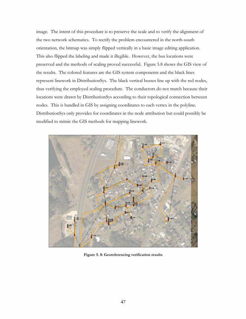
image. The intent of this procedure is to preserve the scale and to verify the alignment of
the two network schematics. To rectify the problem encountered in the north-south
orientation, the bitmap was simply flipped vertically in a basic image editing application.
This also flipped the labeling and made it illegible. However, the bus locations were
preserved and the methods of scaling proved successful. Figure 5.8 shows the GIS view of
the results. The colored features are the GIS system components and the black lines
represent linework in DistributionSys. The black vertical busses line up with the red nodes,
thus verifying the employed scaling procedure. The conductors do not match because their
locations were drawn by DistributionSys according to their topological connection between
nodes. This is handled in GIS by assigning coordinates to each vertex in the polyline.
DistributionSys only provides for coordinates in the node attribution but could possibly be
modified to mimic the GIS methods for mapping linework.
Figure 5. 8: Georeferencing verification results
47

Chapter 6 – Conclusions
Through this effort, it is obvious that the integration of GIS and power system
analysis efforts provides added functionality to the management of utility systems. As
competition increases and as information technologies advance, a utility’s data becomes
more and more valuable as a corporate resource. As a result, sharing information becomes
very important to the efficiency of an organization. Though this research documents a
small-scale integration, it highlights the ability of GIS to initiate full integration of electric
utility information. The technique of integration and the role of GIS within the envelope of
the entire information system can take many forms. However, through this research it is
apparent that on a basic level, incorporating a spatial component to power systems analysis
extends the capability into new areas.
More specifically, the integration with DistributionSys could be easily coordinated by
the creators of the software. Since DistributionSys is currently utilizing tabular data storage
for the entire model, it would be possible to coordinate the database with GIS to extend the
capability of the software. In its simplest form, DistributionSys could utilize Microsoft
Access for its primary template and its reporting mechanism. This simple step could greatly
enhance the capabilities of the tool. Chapter Seven will further detail suggestions for future
work.
48

Chapter 7 – Suggestions for Future Work
Because it is built upon a relational database structure and because of its ability to
freely import and export tabular information, DistributionSys could be easily extended to
interface more efficiently with Geographic Information Systems. At this point in the
evolution of GIS software, the Access database (.mdb) is the foundation for the personal
geodatabase. For smaller GIS applications or for further academic exercises, the formatting
and reporting capabilities could be coordinated between the personal geodatabase and the
DistributionSys network. This could produce automated transfers of information from one
model to the other. The research documented in this paper demonstrates the basic
interoperability and was accomplished manually with minor re-formatting.
Work could be extended to enable GIS as the Graphical User Interface into the
network analysis capabilities of an engineering software package such as DistributionSys.
The GIS could be the main reporting mechanism for DistributionSys. In the optimal
situation, both software packages would be utilized to their respective strengths. For
example, the mathematical analysis required for load-flow iterations, short-circuit potential,
and voltage drop calculations could easily be performed in the background by
DistributionSys and the system information required as input for these analyses could be
housed in a database structure accessible to both GIS and to DistributionSys. The reporting
could be delivered through the GIS map interface for both tabular and spatial information.
The main objective through an automated integration would be to allow comparison
of DistributionSys data to other, seemingly unrelated systems. For example, once the
automated integration is possible, a user may be able to ask questions such as:
*What is the optimum placement in the distribution system for distributed
generation based on electrical parameters and based on proximity to existing fuel
infrastructure [2]?
*What would be the best place to expand the system both electrically and based on
existing land-use or zoning restrictions?
*Where is the optimum placement for a pad-mounted capacitor bank, based on
necessary voltage support and existing road infrastructure (for delivery)?
*Where is the nearest telecommunication hub for monitoring and control of remote
switchgear, protective devices, or generators?
49

The integration between GIS and engineering software packages could provide
valuable scenario modeling for limitless applications.
In addition, this research identified a minor need for modeling three phase
configurations with commercial, off-the-shelf GIS. This could be created as an open-source
tool written in Visual Basic to extend the capabilities of GIS.
Finally, work could be undertaken to model the IEEE Feeders in GIS utilizing
different data models such as SDSFIE, ESRI, or the IEC Common Information Model. A
comparison of the data standards could provide valuable insight into the differences between
the various system models.
50

References
[1] Interpreting GIS data for operation and control of distribution
networks Wang, Z.; Julian, D.E.; Bass, M.; Peterson, W. Power Systems Conference and Exposition, 2004. IEEE PES, Vol., 10-13 Oct. 2004. Pages: 907- 912, vol.2.
[2] Powerful planning tools Ramirez-Rosado, I.J.; Fernandez-Jimenez, L.A.; Monteiro, C.; Miranda, V.; Garcia-Garrido, E.; Zorzano-Santamaria, P.J. Power and Energy Magazine, IEEE, Vol.3, Iss.2, March-April 2005 Pages: 56- 63. [3] GIS based distribution simulation and analysis Trussell, L.V. Electricity Distribution, 2001. Part 1: Contributions. CIRED. 16th International Conference and Exhibition on (IEE Conf. Publ. No. 482), Vol.5, 2001; Pages: 18-21. [4] Vegetation Management Solution for High Voltage Transmission Lines: New York Power Authority ©ESRI Energy Currents; Fall 2004. [5] Land Records Management for Power Generating Company: American Electric Power Property Information System ©ESRI Energy Currents; Spring 2004. [6] Hurricane Response and Recovery: Foresight Aids Fast Recovery from Disaster ©ESRI Energy Currents; Spring 2004. [7] Environmental Management for Brazil Power Company: Companhia Paranaense de Energia ©ESRI Energy Currents; Summer 2004. [8] Integration Models for GIS Based Network Simulation and Analysis Trussel, Larry; Kenney, Jeff Geospatial Information & Technology Association Annual Conference Technical Session for Systems Integration; March [9] Radial distribution test feeders Kersting, W.H. Power Engineering Society Winter Meeting, 2001. IEEE vol.2, pages.908-912.
51

[10] CIM Extensions to Electrical Distribution and CIM XML for the IEEE Radial Test Feeders Wang, Xiaofeng; Schulz, Noel N.; Neumann, Scott IEEE Transactions on Power Systems Vol. 18, No.3, August 2003.
[11] Utility applications should be integrated with an interface based on a canonical data model, not directly with each other Robinson, G.; Zhou, M.J., Power Systems Conference and Exposition, 2004. IEEE PES Pages.1592- 1596 vol.3, 10-13 Oct. 2004. [12] ArcGIS® Electric Distribution Model Copyright © Environmental Systems Research Institute, Inc. and Miner & Miner, 2001.
[13] Spatial Data Standards for Facilities, Infrastructure, and the Environment: History of Development and Benefits
CADD/GIS Technology Center, U.S. Army Research and Development Center; Vicksburg, Mississippi;
Updated for SDSFIE Release 2.50; October 2005.
[14] https://tsc.wes.army.mil/
[15] Evaluation of the CADD/GIS Project for Utilities Management at NASA LaRC Jones, Sharon Prepared for: Capital Investment Planning Office/Research Facilities Management Organization; Summer 2003. [16] DistributionSys, Version 4.01 Martínez del Sol, Alexis; University of Guadalajara, Mexico.
[17] Elements of Power System Analysis, 4th ed. Stevenson, Jr. William D. McGraw Hill, 1982.
[18] Application of automated mapping system to distribution transformer
load management Yen-Ting Chao; Shen-Ta Lee; Hong-Chan Chang Transmission and Distribution Conference and Exhibition 2002: Asia Pacific. IEEE/PES, Vol.2, 6-10 Oct. 2002 Pages: 1179- 1184, vol.2.
52

Vita
Philip Smith is a native of the Eastern Shore of Virginia. In May 2000, he received
his Bachelor’s degree in Environmental Science from Virginia Tech with a focus on water
resources. Upon graduation, he went to work for the University of Virginia (UVA) in
support of a National Science Foundation, Long-Term Ecological Research center in Oyster
on the Eastern Shore. He worked for UVA for two and a half years as a marine scientist
supporting GPS surveying, GIS analysis, and boat operations throughout the Virginia Coast
Reserve. In February 2003, Philip began working for the National Aeronautics and Space
Administration (NASA) under a cooperative agreement for the Facilities Management
Branch at Wallops Flight Facility. Through this arrangement, he worked as an engineer at
Wallops and undertook a Master’s of Science in power systems at Virginia Tech. Alternating
periods of study and work with NASA, Philip transitioned into his role as an engineering
project manager, electrical distribution system co-owner, GIS Team Leader, and assistant
energy manager for Wallops’ Facilities Management Branch. He conducted his Master’s
work under the direct supervision of Dr. Jaime De La Ree and with the guidance of Dr.
Virgilio Centeno and Dr. Yilu Liu. Philip Smith completed his M.S. in Electrical
Engineering in December 2005 and immediately converted to work as a civil-servant project
manager at Wallops Flight Facility.
53