Submission for Computer Applications in Engineering Education

Title: Practical Case Studies for Undergraduate Process Dynamics and ControlUsing the Process Control Modules (PCM)

Authors: Francis J. Doyle III, Edward P. Gatzke, Robert S. Parker

Author Affiliations: Department of Chemical EngineeringUniversity of DelawareNewark, DE 19716

All correspondence should be addressed to: Francis J. Doyle, email: doyle@che.udel.eduphone: (302) 831-0760, fax: (302) 831-0457

Practical Case Studies for Undergraduate Process Dynamics and Control Using theProcess Control Modules (PCM)

Francis J. Doyle III, Edward P. Gatzke, Robert S. Parker

Department of Chemical EngineeringUniversity of DelawareNewark, DE 19716

Abstract: An effective environment for the incorporation of realistic case studies isintroduced for a process dynamics and control course. The Process Control Modules(PCM) can be used in a computer laboratory under MATLAB 5.1 and Simulink 2.1(Mathworks). Several industrial case studies are reviewed which exemplify the useof such a tool for control education.

Keywords: Process Control Education, MATLAB/ SIMULINK, Chemical Engineering,Process Simulation

INTRODUCTION

The need for decreased variance in product quality coupled with tighterenvironmental regulation in the chemical process industries motivates improved processcontrol of both existing processes and systems under development. Industrial demand forbetter process control implies that a detailed understanding of process control issues isexpected of undergraduate students entering the workforce. Typical undergraduateprocess control classes are very mathematical, with lectures focusing mostly on the theoryof modeling, design, and analysis. Many students find control theory concepts difficult tocomprehend. A process control laboratory which can demonstrate and motivate the ideaspresented in lecture is one effective means for transferring the knowledge to the students.

There are many different objectives to be considered when developing a processcontrol laboratory. Theoretical concepts should be presented in a realistic andunderstandable manner. Students should find the covered topics to be well motivated andclearly applicable in the real-world. A control laboratory with multiple unit operationscontrolled by a DCS would certainly demonstrate industrial principles and methods to thestudents, but this type of laboratory would be prohibitive to many universities because ofeconomics, safety, and operation time constraints. Distance learning may also factor intothe course laboratory objectives. A good solution for all of these concerns is thedevelopment of computer simulations which realistically demonstrate theoretical issues tostudents.

There are other similar software packages which are currently available. Cooper[1], Koppel [2], Marlin [3], and Bequette [4, 5] have developed software packages forprocess control education. With the exception of [3] and [4, 5], these packages do nothandle realistic large scale problems in an open programming environment (such asMATLAB).

PROCESS CONTROL MODULES

The Process Control Modules (PCM) package is comprised of many units, eachcovering a different topic in process dynamics and control. Most of the modules focus onthe modeling or control of a typical chemical engineering unit operation. Currently, fourdifferent process models are available with PCM. These include a heated tube furnace, abinary distillation column, a continuous fermentation biological reactor, and a continuousKraft pulp digester. In each of these cases, a detailed fundamental process description isemployed These realistic case studies serve as a valuable component in the controlcurriculum.

PCM is a flexible package. Each module is largely independent of the others, so aninstructor can elect to use a subset of the modules for assignments. New unit operationmodels can also be quickly added. For example, a company may want to use PCM to holda process control course for employees using a model of their existing operation instead ofthe models provided with PCM. Advanced controller designs can be incorporated intoPCM for use in graduate level control classes. PCM is also flexible in that it will run onany platform supported by MATLAB (Win 95, Win NT, Mac, UNIX).

A manual is included with the PCM software. This manual provides information,detailed software directions, and student simulation exercises related to the module topic.The manual explains how to run the PCM software on a very detailed level, assuming thatthe students have no prior experience with MATLAB and SIMULINK. The manualcontains basic information about different elementary process control topics, but it is notintended as a replacement for a standard textbook. Each laboratory module is subdividedinto four sections: objective, introduction, exercises, and summary. In addition, eachmodule includes a section entitled “Things to Think About” which is essentially a pre-lab,or set of exercises, for the students to complete before running the simulations. Thissection helps to orient students to the unit’s topic and introduce concepts related to thecurrent module.

Short descriptions of the topics currently covered by the Process Control Modulesare included in the following section. It is worth noting, that all of the units (except theIntroduction and the First and Second Order Systems) deal with a specific case study. Inthe offerings of this laboratory by the first author at both Purdue University and theUniversity of Delaware, several unit operations have been rotated into the computerlaboratory on a annual basis.

PCM Module Descriptions

Introduction. This laboratory module introduces the students to MATLAB andSIMULINK. Elementary command line exercises and block diagram simulations are

performed. The students also learn how to start modules using the mainmenu graphicaluser interface (Figure 1). This module is independent of a particular unit operation.

Steady-State Gains. This is the first module to focus on a particular unit operation.Students change values for system inputs in a SIMULINK window. The system outputlevels are displayed in the simulation process monitor window (Figure 2). Students canuse a click and point interface to ascertain process variable values from the strip chartwindows. After collecting step change data, the students can then calculate steady-stategains for the unit operation. The operating point is then changed and gains arerecalculated. This demonstrates to students the nonlinear effects typical of an actualprocess. The students also calculate and evaluate steady-state control moves, given aknown disturbance and desired output change.

First and Second Order Systems. In this module, students explore the dynamiccharacteristics of first and second order transfer functions. Students are presented aSIMULINK simulation window and a monitor which displays the system input and outputvalues. From the time domain response to an input step change, the students calculaterelevant system parameters. For first-order systems, this includes the gain and timeconstant. For second order systems, the students determine values for the gain, naturalperiod, dampening coefficient, overshoot, and decay ratio. After exposure to the variouseffects of parameter variation, the students are presented with several unknown problemsand are asked to identify the system parameters. While the processes employed in theseunits are low order (first and second order, e.g. surge tanks), the students are given achance to familiarize themselves with the graphical nature of the SIMULINK interfacebefore being introduced to the more complex case studies.

Transient Response. This unit demonstrates the development of transfer function modelsfrom step test data. The students collect data from step changes applied to one of the casestudies. The data is displayed using PCMplot, a PCM-specific graphical tool for processmodeling, identification and validation (Figure 3). This data is analyzed to develop first-order models with a time-delay. Due to the high order nature of the underlying nonlinearprocess dynamics and the random noise signal applied to the process measurements, thestudents are exposed to the kind of realistic data they would encounter in practice at achemical plant, refinery, mill, etc.. Hence, they will find that a first-order (plus delay)model is very simple from a computational perspective, but it is at best an approximationto a real system. In the course of the model identification, students develop a transferfunction simulation in SIMULINK. Given the original process data, and data generated bytheir identified model, students can validate the model fidelity using PCMplot.

Open Loop Frequency Response. Frequency response techniques can give studentspowerful tools for use in industry. In this module, students learn how to create afrequency response model. Classic textbook treatment of this problem uses sinusoidalforcing of the process to generate individual frequency points, however this is hardly everdone in practice. The more practical approach involves a transformation of time-domain(discrete) data into frequency domain data. This is accomplished using pulse-testing along

with a fast-fourier transformation. The pcmfft command performs the fourier transform,and the plot_bode command creates a Bode plot (Figure 4) with chemical engineeringunits. Initially, the students create bode plots from first and second-order transferfunctions. The same exercise is repeated using the unit operation model. As with theprevious identification unit, the students encounter all the practical limitations of finitemagnitude inputs, finite duration signals, noise-corrupted data, and complex dynamicprocess behavior. The Bode plots which result from the case study do not display the niceproperties of low order systems (as seen in the slope of the high frequency asymptote ofthe amplitude ratio). Therefore the students must exercise engineering judgment indeveloping an approximate model that is consistent with their data and is suitable forsubsequent controller design.

Steady State Analysis of Feedback Control. This laboratory module introduces theconcept of feedback control. The students use the models generated in the transientresponse module to develop PID tuning constants using standard tuning rules. Usingsetpoint changes and disturbance loading, the students examine the effect of integral actionon steady-state system control.

PID Controller Tuning. This unit allows the students to explore the dynamic responseof a process case study using PID feedback controllers. The students introduce stepchanges and disturbances to the system and monitor the output variable response. Usingthe models developed earlier (transfer function and frequency domain), the students applythree distinct tuning algorithms and compare the results. These algorithms include Cohen-Coon, Ziegler-Nichols, and relay tuning. The latter tuning approach is important as itrepresents a modern approach to control tuning which is available in many commercialcontrol packages, but is only treated in the most current undergraduate textbooks. Itsefficacy for a complex system, for which the other two tuning methods fail, is highlightedin this unit.

Feed-Forward control. Using the process models developed in the transient responsemodule, students develop, implement, and test feed-forward control designs. Again, theprinciple of approximation is reinforced, as the students learn that simple lead-lag feed-forward controllers do not exactly cancel the responses of complex systems. However, thestudents find that even simple approximations can be highly effective in the anticipatoryresponse provided by feed-forward control.

IMC and Multivariable Control. In this unit, the system process model is used todevelop an Internal Model Control (IMC) controller. This module highlights the role ofadvanced model-based design methods for controller synthesis. Once again relatively fewtextbooks address this approach at the undergraduate level, but the concepts arestraightforward, and the application in the laboratory can significantly reinforce thelearning. The tuning procedure is reduced to two intuitive time constants (one per loop),and the students find that low order model approximations can serve as valuablecomponents in a direct synthesis controller design method. The second half of this labintroduces multivariable control design using a decoupling approach.

Model Predictive Control. This module demonstrates Model Predictive Control (MPC),also known as Dynamic Matrix Control (DMC). The transfer function models obtained inearlier modules are discretized to develop a discrete step-response model. This controllerdesign methodology is considered by many to be the current state of the art in advancedcontrol design, and it gives the students a brief introduction to the important issues. It alsoraises the important issue of digital computing, and the role of optimization in solvingcontrol problems. The tuning procedure becomes more complicated, as it would for anyrealistic case study. The students are challenged to find suitable values for the horizonsused in MPC (move and prediction), as well as the weighting matrices (input and output).

PCM Unit Operations

Typical Unit. Any process unit operation with a continuous finite state space realizationcan be modeled in the SIMULINK environment. The PCM laboratory modules currentlymake use of four fundamental models, but new modules can easily be developed for usewith different unit operations. Ideally, a new unit operation would have at least fourinputs and four outputs. Two of the inputs should be manipulated variables and the othertwo should be disturbance variables. For feed-forward control purposes, one of thedisturbance inputs should be a variable that could be realistically transmitted by a fieldsensor. The SIMULINK block for any new unit operation should use absolute processvariables for inputs and outputs. A process model should take less than ten actual minutesto simulate an input step change response, otherwise its value in the laboratory classroomwill be limited. The student interface to a typical unit is shown in Figure 5, where it isevident that the student has convenient access during run-time to parameter values in theprocess (inputs, tuning parameters, etc.) through a convenient graphical environment.

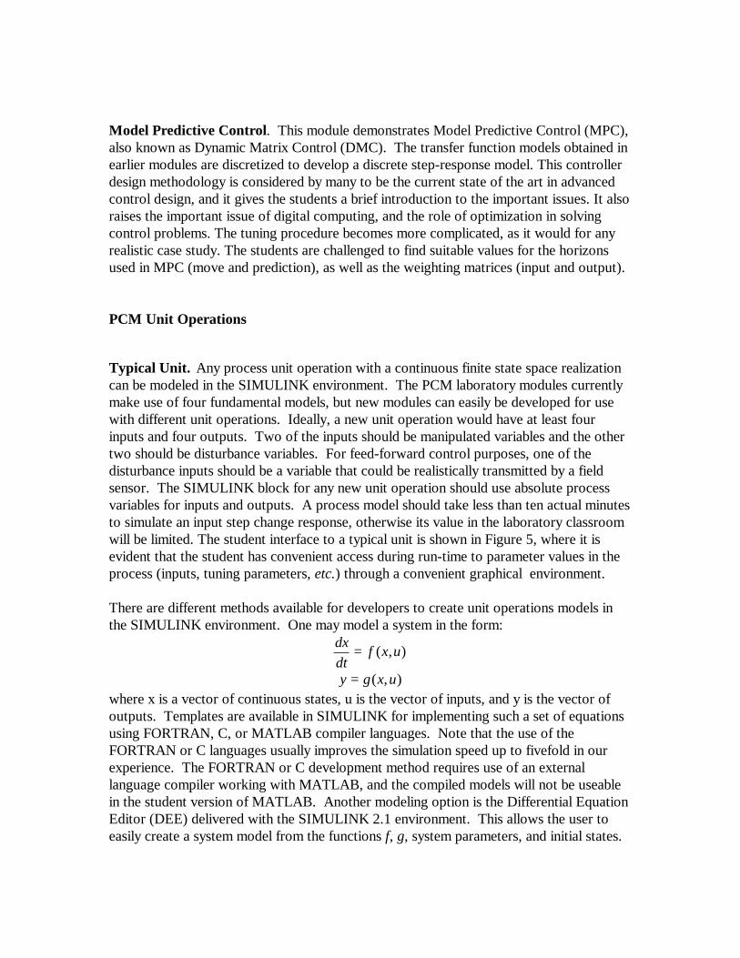
There are different methods available for developers to create unit operations models inthe SIMULINK environment. One may model a system in the form:

),( uxfdtdx =

),( uxgy =where x is a vector of continuous states, u is the vector of inputs, and y is the vector ofoutputs. Templates are available in SIMULINK for implementing such a set of equationsusing FORTRAN, C, or MATLAB compiler languages. Note that the use of theFORTRAN or C languages usually improves the simulation speed up to fivefold in ourexperience. The FORTRAN or C development method requires use of an externallanguage compiler working with MATLAB, and the compiled models will not be useablein the student version of MATLAB. Another modeling option is the Differential EquationEditor (DEE) delivered with the SIMULINK 2.1 environment. This allows the user toeasily create a system model from the functions f, g, system parameters, and initial states.

Furnace. This model was originally developed in 1982-1983 under the direction ofProfessor Lowell Koppel for use in the IBM Advanced Control System (ACS)instructional modules at Purdue University. The system models the heating of a high-molecular weight hydrocarbon feed to a cracking unit of a refinery. An air-fuel mixtureundergoes combustion in the furnace to heat the hydrocarbon feed. The furnace modelhas 26 continuous states, with a detailed description given in Appendix A. The furnacehas two manipulated process inputs: air flow rate and fuel gas flow rate. There are fivedisturbance inputs: hydrocarbon inlet temperature, hydrocarbon flow rate, air temperature,fuel gas temperature, and fuel gas purity. The measured process variables arehydrocarbon outlet temperature, furnace temperature, exhaust gas flow rate, and oxygenexit temperature.

This unit is particularly effective in demonstrating the effect of transport delay through adistributed parameter system, and the disparate time scales associated with mass andenergy effects in a reactor.

Binary Distillation Column. This unit operation models the separation of a mixture ofethanol and methanol. The column has 27 trays with a reboiler on the bottom tray and atotal condenser on the overhead stream. This model was originally developed at theUniversity of Maryland [6]. Manipulated process inputs are reflux ratio and vapor flowrate. The feed methanol mole fraction and feed flow rate act as disturbance inputs. Themeasured process outputs are: overhead methanol mole fraction, overhead product flowrate, bottom methanol flow rate, and bottom product flow rate. This model has 60continuous states.

This unit is most effective for demonstrating the interactive nature of multivariableprocesses, as well as the nonlinear nature of high purity columns in the limit of high refluxor vapor boilup.

Biological Reactor. This unit operation is a seven state model of a continuous flowfermentation biological reactor. A biological organism (SACCHAROMYCESCEREVISIEA) is contained in a CSTR with a glucose solution feed stream. The model istaken from [7, 8]. There are seven states in the model. The manipulated process inputsare dilution rate and glucose feed concentration. Disturbance inputs are specific glucoseuptake rate and growth rate. The outputs are cell biomass concentration, exit glucoseconcentration, and ethanol concentration.

This unit represents one of the more modern unit operations that have appeared in thechemical engineering curriculum. It can be easily modified to accommodate otherorganisms and metabolic pathways.

Pulp Digester. This process is the key unit operation at the front end of a pulp mill, inwhich the wood chips are broken down using a caustic liquor. The control objectiveinvolves the regulation of the final pulp properties, despite upsets in the biologicalfeedstock properties. The computer model is derived from [9, 10] and employs over 1000

dynamic states in representing the distributed parameter behavior through a lumped (seriesof CSTRs) approximation. The inputs include upper extract flowrate, cookingtemperature, MCC temperature, MCC trim flowrate, chip flowrate, and chip moisture.The outputs are kappa number, upper and lower effective alkali, and lower Na2Sconcentration.

This unit exposes students to another sector of the industry that is often under-representedin the chemical engineering curriculum, but is a large employer of chemical engineers – thepulp and paper industry. Furthermore it highlights the challenges of working with longtime delay systems (~ 6-8 hours).

FUTURE WORK

There are a number of ongoing efforts to develop and improve the PCM package.In the next year, there will be two notable enhancements to the graphical interface. TheMATLAB GUI design tool (GUIDE) will be used to reformat the process monitorwindows, and provide easier user access to simulation parameters. PCM development isalso exploring the use of multimedia. This will make PCM a more powerful learningexperience by providing audio and visual instruction to supplement the current workbookand simulation. The new multimedia content of PCM will offer information andexplanations about different process control and PCM topics. The content will also allowthe development of a plant-like operating environment. For example, this may beaccomplished by providing a video of an operator adjusting a valve in a plant or creatingwarning bells when process constraints are violated. The interactive experience will helpto capture the attention of the student, increasing the retention and understanding of thematerial.

CONCLUSIONS

The Process Control Module system provides students with an opportunity for ahands-on, realistic, computer laboratory experience. Use of fundamental models exposesstudents to conditions that would be observed in actual process systems, such as nonlinearsystem gains, high order dynamics and noise-corrupted measurements. MATLAB andSIMULINK allows PCM to support any MATLAB supported platform (Win95, WinNT,Mac, UNIX). The SIMULINK environment allows for easy development, modification,and extension of the current package.

ACKNOWLEDGMENTSThe authors acknowledge the support of the following students who have helped

develop the PCM software: Atsushi Aoyama, Arda Bafra, Lalitha Balasubramhanya,Derek Brown, Clark Case, Jorge Castrove, Matthew Clamme, Joseph Cooper, MarutiDey, Edward Gatzke, Jason Gause, Douglas Heemstra, Steven Honkomp, Jeffrey Kao,Thomas Kendi, Daniel King, Harpreet Kwatra, Alan Mahoney, Bryon Maner, Kerry Need,Robert Parker, Anh Phung, Kairali Podual, Andre Shaw, Alexander Stack, PhillipWisnewski, and Stanley Wrobel.

ADDITIONAL INFORMATION ABOUT PCM

Interested educators are referred to the Web-page for the Process Control Modules at:http://www.che.udel.edu/pcm

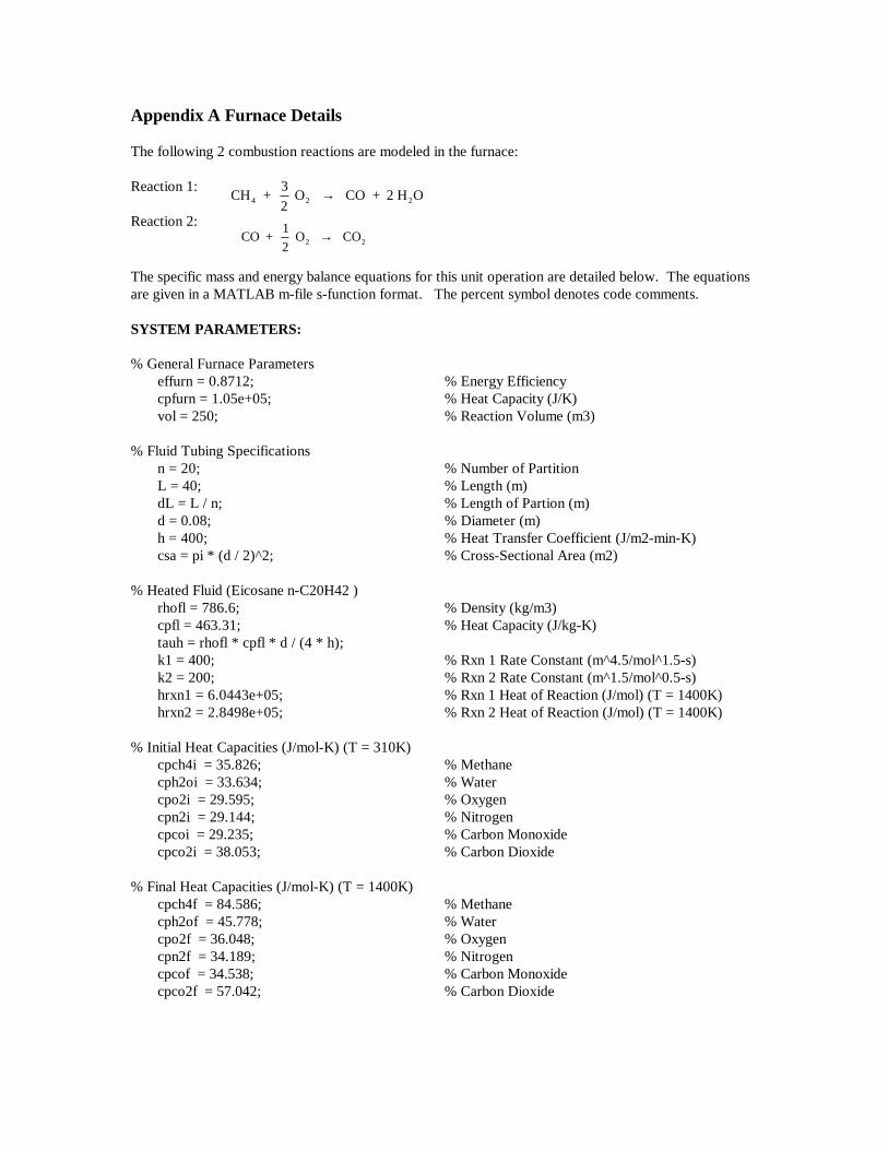
Appendix A Furnace Details

The following 2 combustion reactions are modeled in the furnace:

Reaction 1:

Reaction 2:

The specific mass and energy balance equations for this unit operation are detailed below. The equationsare given in a MATLAB m-file s-function format. The percent symbol denotes code comments.

SYSTEM PARAMETERS:

% General Furnace Parameters effurn = 0.8712; % Energy Efficiency cpfurn = 1.05e+05; % Heat Capacity (J/K) vol = 250; % Reaction Volume (m3)

% Fluid Tubing Specifications n = 20; % Number of Partition L = 40; % Length (m) dL = L / n; % Length of Partion (m) d = 0.08; % Diameter (m) h = 400; % Heat Transfer Coefficient (J/m2-min-K) csa = pi * (d / 2)^2; % Cross-Sectional Area (m2)

% Heated Fluid (Eicosane n-C20H42 ) rhofl = 786.6; % Density (kg/m3) cpfl = 463.31; % Heat Capacity (J/kg-K) tauh = rhofl * cpfl * d / (4 * h); k1 = 400; % Rxn 1 Rate Constant (m^4.5/mol^1.5-s) k2 = 200; % Rxn 2 Rate Constant (m^1.5/mol^0.5-s) hrxn1 = 6.0443e+05; % Rxn 1 Heat of Reaction (J/mol) (T = 1400K) hrxn2 = 2.8498e+05; % Rxn 2 Heat of Reaction (J/mol) (T = 1400K)

% Initial Heat Capacities (J/mol-K) (T = 310K) cpch4i = 35.826; % Methane cph2oi = 33.634; % Water cpo2i = 29.595; % Oxygen cpn2i = 29.144; % Nitrogen cpcoi = 29.235; % Carbon Monoxide cpco2i = 38.053; % Carbon Dioxide

% Final Heat Capacities (J/mol-K) (T = 1400K) cpch4f = 84.586; % Methane cph2of = 45.778; % Water cpo2f = 36.048; % Oxygen cpn2f = 34.189; % Nitrogen cpcof = 34.538; % Carbon Monoxide cpco2f = 57.042; % Carbon Dioxide

CH + 32

O CO + 2 H O 4 2 2→

CO + 12

O CO 2 2→

SYSTEM INPUTS:

% u(1) = Hydrocarbon Fluid Flow Rate (m3/min), ss=0.035% u(2) = Hydrocarbon Inlet Temperature (K), ss=310% u(3) = Air Flow Rate (m3/min), ss=17.9% u(4) = Air Temperature (K), ss=310% u(5) = Fuel Gas Flow Rate (m3/min), ss=1.21% u(6) = Fuel Gas Temperature (K), ss=310% u(7) = Fuel Gas Purity (moles CH4/mole), ss=1

ALGEBRAIC AND STATE EQUATIONS:

rhoig = P / (R * u(4)); % Ideal Gas Density (mol/m3) feed = u(3) + u(5); % Combustion Reactants Feed Rate (m3/min) velfl = u(1) / csa; % Velocity of Fluid (m/min)

% Initial Concentrations (mol/m3) cch4i = u(7) * u(5) * rhoig / feed; % Methane ch2oi = (1 - u(7)) * u(5) * rhoig / feed; % Water co2i = 0.21 * u(3) * rhoig / feed; % Oxygen cn2i = 0.79 * u(3) * rhoig / feed; % Nitrogen ccoi = 0; % Carbon Monoxide cco2i = 0; % Carbon Dioxide

% Initial Species Flow Rates (mol/s) nch4i = cch4i * feed; % Methane nh2oi = ch2oi * feed; % Water no2i = co2i * feed; % Oxygen nn2i = cn2i * feed; % Nitrogen ncoi = 0; % Carbon Monoxide nco2i = 0; % Carbon Dioxide

% Final Species Flow Rates (mol/s) nch4f = nch4i - k1 * x(1) * x(3) ^ 1.5 * vol; % Methane nh2of = nh2oi + 2 * k1 * x(1) * x(3) ^ 1.5 * vol; % Water no2f = no2i - 1.5 * k1 * x(1) * x(3) ^ 1.5 * vol - 0.5 * k2 * x(4) * x(3) ^ 0.5 * vol; % Oxygen nn2f = nn2i; % Nitrogen ncof = k1 * x(1) * x(3) ^ 1.5 * vol - k2 * x(4) * x(3) ^ 0.5 * vol; % Carbon Monoxide nco2f = k2 * x(4) * x(3) ^ 0.5 * vol; % Carbon Dioxide ntotf = nch4f + nh2of + no2f + nn2f + ncof + nco2f; % Total

% Combustion Products Exit Flow (m3/min), from mass balance on carbon exit = (2 * no2i + nh2oi) / (x(2) + 2 * x(3) + x(4) + 2 * x(5));

% Mass Balance of Combustion Species

% Species Concentrations:% Methane x(1), Water x(2), Oxygen x(3), Carbon Monoxide x(4), Carbon Dioxide x(5) dx(1) = (1 / vol) * (nch4i - exit * x(1)) - k1 * x(1) * x(3) ^ 1.5; dx(2) = (1 / vol) * (nh2oi - exit * x(2)) + 2 * k1 * x(1) * x(3) ^ 1.5; dx(3) = (1 / vol) * (no2i - exit * x(3)) - 1.5 * k1 * x(1) * x(3) ^ 1.5 - 0.5 * k2 * x(4) * x(3) ^ 0.5;

dx(4) = (1 / vol) * (ncoi - exit * x(4)) + k1 * x(1) * x(3) ^ 1.5 - k2 * x(4) * x(3) ^ 0.5; dx(5) = (1 / vol) * (nco2i - exit * x(5)) + k2 * x(4) * x(3) ^ 0.5;

% Energy Balance of Combustion Species and Fluid, dT/dt for initial partition dx(1+5) = (velfl / dL) * (u(2) - x(1+5)) + (1 / tauh) * (x(5+n+1) - x(1+5));

% dT/dt for 2nd to nth Partition of Tubing (x(2+5) to x(n+5)) (K/s) for i = (2+5):(n+5) dx(i) = (velfl / dL) * (x(i-1) - x(i)) + (1 / tauh) * (x(5+n+1) - x(i)); end

% Heat Exchange (J/s)% Energy Lost to Species as Enthalpy, (Final - Initial) {-} qi = (nch4i * cpch4i + nh2oi * cph2oi + no2i * cpo2i + nn2i * cpn2i) * u(4); qf = (nch4f *cpch4f+nh2of *ph2of+no2f*cpo2f+nn2f*cpn2f+ncof*cpcof+nco2f*cpco2f)*x(5+n+1);

% Energy Generated by Reactions {+} qrxn1 = effurn * (k1 * x(1) * x(3) ^ 1.5 * vol) * hrxn1; qrxn2 = effurn * (k2 * x(4) * x(3) ^ 0.5 * vol) * hrxn2;

% Energy Lost to Fluid {-} qfluid = h * d * dL * pi * (n * x(5+n+1) - sum(x(5+1:5+n)));

% Energy Balance of Furnace (x(5+n+1), furnace temperature) dx(5+n+1) =(qrxn1 + qrxn2 - (qf - qi) - qfluid) / cpfurn;

References

[1] D. J. Cooper. “Picles ™ : a simulator for ‘virtual world’ education and training inprocess dynamics and control,” Computer Applications in Engineering Education, Vol. 4,No. 3, 1996, pp. 207-215.

[2] L. B. Koppel and G. R. Sullivan. “Use of IBM’s advanced control system inundergraduate process control education,” Chemical Engineering Education, Vol. 20,1986, p 70.

[3] T. E. Marlin. “Software laboratory for undergraduate process control education,”Computers & Chemical Engineering Proceedings of the 6th European Symposium onComputer Aided Process Engineering. Part B. May 26-29 1996, Vol. 20.

[4] B. W. Bequette, K. D. Schott, V.Prasad, V. Natarajan and R.R. Rao. "Case StudyProjects in an Undergraduate Process Control Course," Chemical Engineering Education(in press, 1998).

[5] B. W. Bequette, "Case Study Projects in an Undergraduate Process ControlCourse." Proceedings of Control-97, Sydney, p 212-217 (1997).

[6] K. Weischedel and T. J. McAvoy. “Feasibility of decoupling in conventionallycontrolled distillation columns,” Independent Engineering Chemical Fundamentals, Vol.19, 1980, p 379.

[7] Lievense, Jefferson Clay. “An investigation of the aerobic, glucose-limited growthand dynamics of SACCHAROMYCES CEREVISIEA,” PhD Thesis, Purdue University,1984.

[8] Aoyama Atsushi. “Modeling and control of nonlinear processes using neuralnetworks and fuzzy logic,” PhD Thesis, Purdue University, 1994.

[9] P. A. Wisnewski. “Inferential control using high order process models withapplication to a continuous pulp digester,” PhD Thesis, Purdue University, 1997.

[10] F. Kayihan. “Continuous Digester Benchmark Dynamic Model,” Matlab ToolboxCode, IETek, 1997.

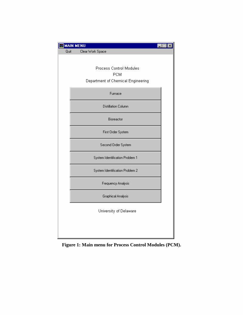
Figure 1: Main menu for Process Control Modules (PCM).

Figure 2: Process monitor for furnace unit, showing capability for data archiving,window control, axis rescaling, and pointer function (with depicted cross-hair).

Figure 3: Interface for PCMPlot utility, showing original process data (yellow solidline) and fitted first-order-plus-time-delay response (blue dash-dot line).

Figure 4: Output of plot_bode command, showing the amplitude ratio (top) andphase lag (bottom) over the frequency range of interest.

Figure 5: Process flowsheet window showing the student interface for real-timeoperation of the furnace