effects of local features of the inflaton potential on the spectrum and bispectrum of primordial...
DESCRIPTION
Effects of local features of the inflaton potential on the spectrum and bispectrum of primordial perturbationsTRANSCRIPT
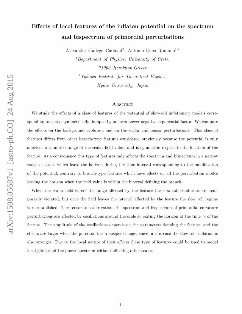
Effects of local features of the inflaton potential on the spectrum
and bispectrum of primordial perturbations
Alexander Gallego Cadavid2, Antonio Enea Romano1,2
1Department of Physics, University of Crete,
71003 Heraklion,Greece
2Yukawa Institute for Theoretical Physics,
Kyoto University, Japan
Abstract
We study the effects of a class of features of the potential of slow-roll inflationary models corre-
sponding to a step symmetrically dumped by an even power negative exponential factor. We compute
the effects on the background evolution and on the scalar and tensor perturbations. This class of
features differs from other branch-type features considered previously because the potential is only
affected in a limited range of the scalar field value, and is symmetric respect to the location of the
feature. As a consequence this type of features only affects the spectrum and bispectrum in a narrow
range of scales which leave the horizon during the time interval corresponding to the modification
of the potential, contrary to branch-type features which have effects on all the perturbation modes
leaving the horizon when the field value is within the interval defining the branch.
When the scalar field enters the range affected by the feature the slow-roll conditions are tem-
porarily violated, but once the field leaves the interval affected by the feature the slow roll regime
is re-established. The tensor-to-scalar ration, the spectrum and bispectrum of primordial curvature
perturbations are affected by oscillations around the scale k0 exiting the horizon at the time τ0 of the
feature. The amplitude of the oscillations depends on the parameters defining the feature, and the
effects are larger when the potential has a steeper change, since in this case the slow-roll violation is
also stronger. Due to the local nature of their effects these type of features could be used to model
local glitches of the power spectrum without affecting other scales.
1
arX
iv:1
508.
0568
7v1
[as
tro-
ph.C
O]
24
Aug
201
5
I. INTRODUCTION
Theoretical cosmology has entered in the last decades in a new era in which different models
can be compared directly to observations [1–4]. One fundamental source of information about
the early Universe is the cosmic microwave background (CMB) radiation, which according
to the standard cosmological model consists of photons which decoupled from the primordial
plasma when the neutral hydrogen atoms started to form.
According to inflation theory [5] the CMB temperature anisotropies arose from primordial
curvature perturbations. In slow-roll inflationary models the primordial curvature perturbations
are expected to be highly gaussian, with a non gaussian component of the order of the slow-roll
parameters [6]. The most recent CMB observations are compatible with some non Gaussianity
corresponding to f localNL = 2.5 ± 5.7 and f equilNL = −16 ± 70 [7–10], motivating the theoretical
study of the conditions which could have generated it. Some recent developments in the study of
models which could generate non Gaussianity and on their detection can be found for example in
[11–15]. Among the different mechanisms that could have generated primordial non gaussianity
there is the temporary violation of the slow-roll conditions [1], which could for example be
produced by a local feature of the inflaton potential. The effects of features of the inflaton
potential was first studied by Starobinsky [16], and CMB data have shown some glitches of the
power spectrum [17, 18] compatible with these features [19–22].
The Starobinsky model and its generalizations [23, 24] belong to a class of branch features
(BF) which involve a step function or a smoothed version of the latter [25], and consequently
introduce a distinction between a left and right branch of the potential. In this paper instead we
will consider the effects of local features (LF) [26] which only modify the potential locally in field
space, while leaving it unaffected sufficiently far from the feature. The important consequence
is that also the effects of LF on the spectrum and bispectrum are local, while BF modify the
spectrum in a wider range of scales. Features of the inflaton potential could be produced by
for example particle production [27], or phase transitions [28], but here we will only study their
effects adopting a phenomenological approach as done originally by Starobinsky in its seminal
work.
2
1.0 1.1 1.2 1.3 1.4 1.5
Φ
Φ0
1.0002
1.0004
1.0006
1.0008
1.0010
VF
V0
1 2 3 4 5
Τ
Τ0
-3. ´ 10-8
-2. ´ 10-8
-1. ´ 10-8
1. ´ 10-8
2. ´ 10-8
3. ´ 10-8
DH
1 2 3 4
Τ
Τ0
0.0150
0.0155
0.0160
0.0165
0.0170
0.0175
0.0180
Ε
1 2 3 4
Τ
Τ0
-0.5
0.0
0.5
Η
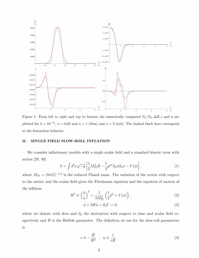
Figure 1: From left to right and top to bottom the numerically computed VF /V0,∆H, ε and η are
plotted for λ = 10−11, σ = 0.05 and n = 1 (blue) and n = 2 (red). The dashed black lines correspond
to the featureless behavior.
II. SINGLE FIELD SLOW-ROLL INFLATION
We consider inflationary models with a single scalar field and a standard kinetic term with
action [29, 30]
S =∫d4x√−g
[1
2M2
PlR−1
2gµν∂µφ∂νφ− V (φ)
], (1)
where MPl = (8πG)−1/2 is the reduced Planck mass. The variation of the action with respect
to the metric and the scalar field gives the Friedmann equation and the equation of motion of
the inflaton
H2 ≡(a
a
)2
=1
3M2Pl
(1
2φ2 + V (φ)
), (2)
φ+ 3Hφ+ ∂φV = 0, (3)
where we denote with dots and ∂φ the derivatives with respect to time and scalar field re-
spectively and H is the Hubble parameter. The definition we use for the slow-roll parameters
is
ε ≡ − H
H2, η ≡ ε
εH. (4)
3
1.0 1.1 1.2 1.3 1.4 1.5
Φ
Φ0
1.0002
1.0004
1.0006
1.0008
1.0010
VF
V0
1 2 3 4 5
Τ
Τ0
-2. ´ 10-8
2. ´ 10-8
4. ´ 10-8
DH
1 2 3 4
Τ
Τ0
0.0150
0.0155
0.0160
0.0165
0.0170
0.0175
Ε
1 2 3 4
Τ
Τ0
-0.2
0.0
0.2
0.4
0.6
Η
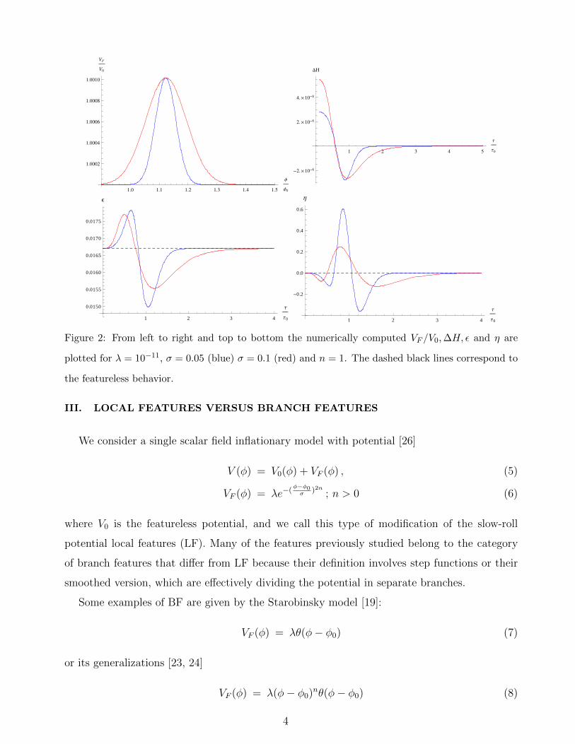
Figure 2: From left to right and top to bottom the numerically computed VF /V0,∆H, ε and η are
plotted for λ = 10−11, σ = 0.05 (blue) σ = 0.1 (red) and n = 1. The dashed black lines correspond to
the featureless behavior.
III. LOCAL FEATURES VERSUS BRANCH FEATURES
We consider a single scalar field inflationary model with potential [26]
V (φ) = V0(φ) + VF (φ) , (5)
VF (φ) = λe−(φ−φ0σ
)2n ; n > 0 (6)
where V0 is the featureless potential, and we call this type of modification of the slow-roll
potential local features (LF). Many of the features previously studied belong to the category
of branch features that differ from LF because their definition involves step functions or their
smoothed version, which are effectively dividing the potential in separate branches.
Some examples of BF are given by the Starobinsky model [19]:
VF (φ) = λθ(φ− φ0) (7)
or its generalizations [23, 24]
VF (φ) = λ(φ− φ0)nθ(φ− φ0) (8)
4
1.0 1.1 1.2 1.3 1.4 1.5
Φ
Φ0
0.9995
1.0000
1.0005
1.0010
VF
V0
1 2 3 4 5
Τ
Τ0
-2. ´ 10-8
-1. ´ 10-8
1. ´ 10-8
2. ´ 10-8
3. ´ 10-8
DH
0.5 1.0 1.5 2.0 2.5 3.0
Τ
Τ0
0.015
0.016
0.017
0.018
Ε
0.5 1.0 1.5 2.0 2.5 3.0
Τ
Τ0
-0.8
-0.6
-0.4
-0.2
0.0
0.2
0.4
0.6
Η
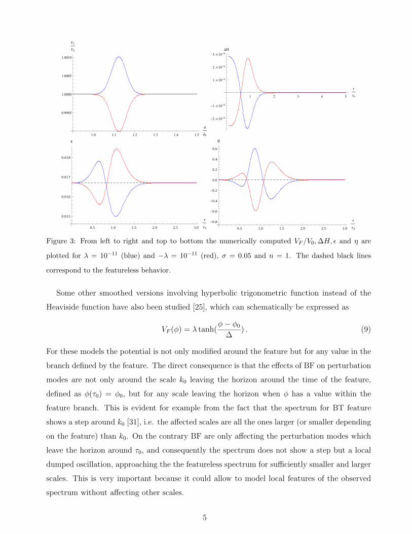
Figure 3: From left to right and top to bottom the numerically computed VF /V0,∆H, ε and η are
plotted for λ = 10−11 (blue) and −λ = 10−11 (red), σ = 0.05 and n = 1. The dashed black lines
correspond to the featureless behavior.
Some other smoothed versions involving hyperbolic trigonometric function instead of the
Heaviside function have also been studied [25], which can schematically be expressed as
VF (φ) = λ tanh(φ− φ0
∆) . (9)
For these models the potential is not only modified around the feature but for any value in the
branch defined by the feature. The direct consequence is that the effects of BF on perturbation
modes are not only around the scale k0 leaving the horizon around the time of the feature,
defined as φ(τ0) = φ0, but for any scale leaving the horizon when φ has a value within the
feature branch. This is evident for example from the fact that the spectrum for BT feature
shows a step around k0 [31], i.e. the affected scales are all the ones larger (or smaller depending
on the feature) than k0. On the contrary BF are only affecting the perturbation modes which
leave the horizon around τ0, and consequently the spectrum does not show a step but a local
dumped oscillation, approaching the the featureless spectrum for sufficiently smaller and larger
scales. This is very important because it could allow to model local features of the observed
spectrum without affecting other scales.
5

1.0 1.1 1.2 1.3 1.4 1.5
Φ
Φ0
1.002
1.004
1.006
1.008
1.010
VF
V0
1 2 3 4 5
Τ
Τ0
-2. ´ 10-8
-1. ´ 10-8
1. ´ 10-8
2. ´ 10-8
3. ´ 10-8
DH
0.5 1.0 1.5 2.0 2.5 3.0
Τ
Τ0
0.0150
0.0155
0.0160
0.0165
0.0170
0.0175
Ε
0.5 1.0 1.5 2.0 2.5 3.0
Τ
Τ0
-0.8
-0.6
-0.4
-0.2
0.0
0.2
0.4
0.6
Η
Figure 4: From left to right and top to bottom the numerically computed VF /V0,∆H, ε and η are
plotted for λ = 10−11 (blue) and λ = 10−12 (red), σ = 0.05 and n = 1. The dashed black lines
correspond to the featureless behavior.
0.1 0.5 1.0 5.0 10.0 50.0 100.0
k
k0
1.8 ´ 10-9
2. ´ 10-9
2.2 ´ 10-9
2.4 ´ 10-9
2.6 ´ 10-9
2.8 ´ 10-9
PΖ
0.1 0.5 1.0 5.0 10.0 50.0 100.0
k
k0
0.24
0.26
0.28
0.3
0.32
0.34
0.36
r
Figure 5: The numerically computed Pζ and r are plotted for λ = 10−11, σ = 0.05 and n = 1 (blue)
and n = 2 (red). The dashed black lines correspond to the featureless behavior.
In this paper we will consider the case of power law inflation (PLI)
V0(φ) = Ae−√
2q
φMPl . (10)
While PLI is not in good agreement with CMB data due to its high value of the tensor-to-
scalar ration r, it can be used as good toy model to show qualitatively the general type of effects
produced by LF. In future works different potentials V0(φ) could be used for direct comparison
6
0.1 0.5 1.0 5.0 10.0 50.0 100.0
k
k0
2. ´ 10-9
2.2 ´ 10-9
2.4 ´ 10-9
2.6 ´ 10-9
2.8 ´ 10-9
PΖ
0.1 0.5 1.0 5.0 10.0 50.0 100.0
k
k0
0.24
0.26
0.28
0.3
0.32
0.34
r
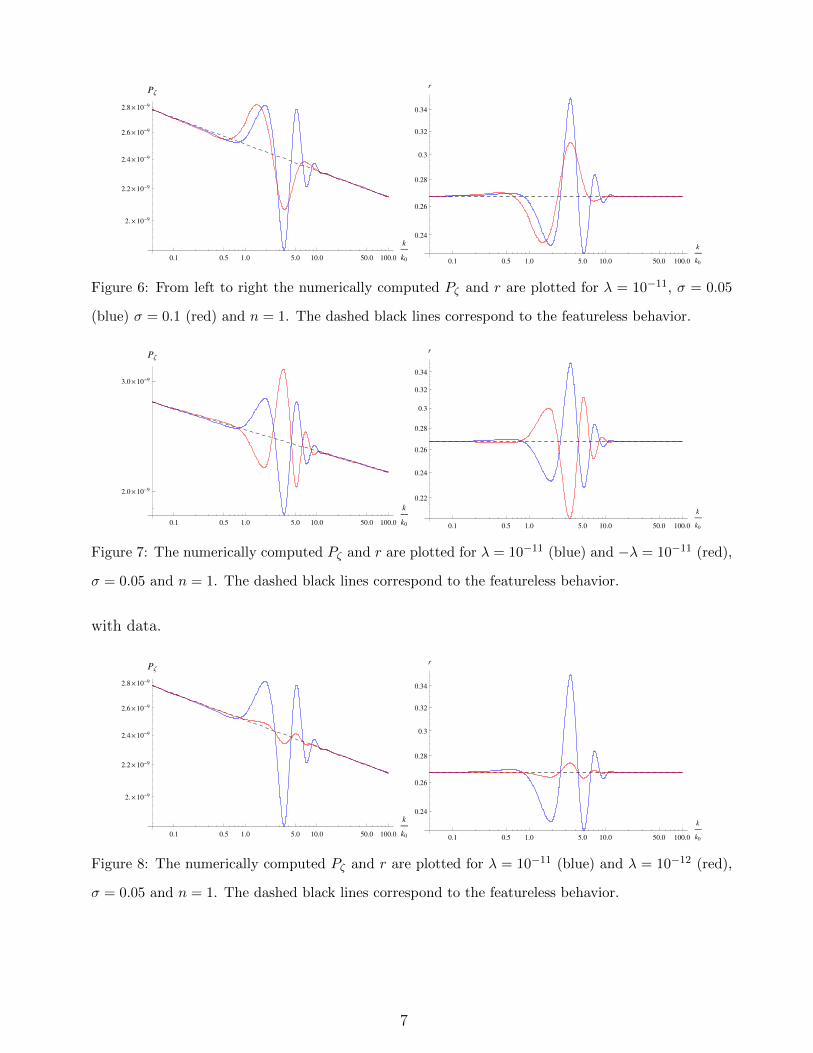
Figure 6: From left to right the numerically computed Pζ and r are plotted for λ = 10−11, σ = 0.05
(blue) σ = 0.1 (red) and n = 1. The dashed black lines correspond to the featureless behavior.
0.1 0.5 1.0 5.0 10.0 50.0 100.0
k
k0
2.0 ´ 10-9
3.0 ´ 10-9
PΖ
0.1 0.5 1.0 5.0 10.0 50.0 100.0
k
k0
0.22
0.24
0.26
0.28
0.3
0.32
0.34
r
Figure 7: The numerically computed Pζ and r are plotted for λ = 10−11 (blue) and −λ = 10−11 (red),
σ = 0.05 and n = 1. The dashed black lines correspond to the featureless behavior.
with data.
0.1 0.5 1.0 5.0 10.0 50.0 100.0
k
k0
2. ´ 10-9
2.2 ´ 10-9
2.4 ´ 10-9
2.6 ´ 10-9
2.8 ´ 10-9
PΖ
0.1 0.5 1.0 5.0 10.0 50.0 100.0
k
k0
0.24
0.26
0.28
0.3
0.32
0.34
r
Figure 8: The numerically computed Pζ and r are plotted for λ = 10−11 (blue) and λ = 10−12 (red),
σ = 0.05 and n = 1. The dashed black lines correspond to the featureless behavior.
7
-2 -1 0 1 2 3 4
logk
k0
-4
-2
0
2
4
FNL
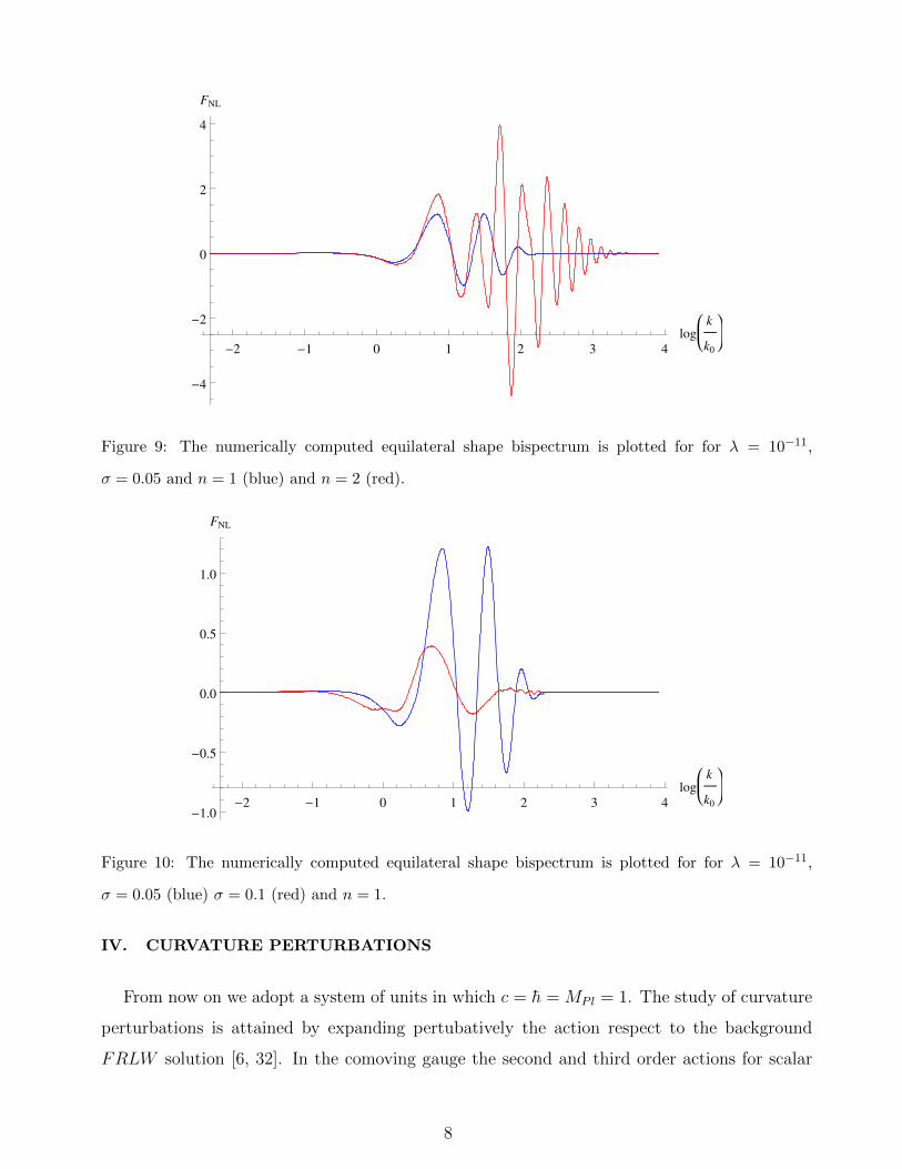
Figure 9: The numerically computed equilateral shape bispectrum is plotted for for λ = 10−11,
σ = 0.05 and n = 1 (blue) and n = 2 (red).
-2 -1 0 1 2 3 4
logk
k0
-1.0
-0.5
0.0
0.5
1.0
FNL
Figure 10: The numerically computed equilateral shape bispectrum is plotted for for λ = 10−11,
σ = 0.05 (blue) σ = 0.1 (red) and n = 1.
IV. CURVATURE PERTURBATIONS
From now on we adopt a system of units in which c = h = MPl = 1. The study of curvature
perturbations is attained by expanding pertubatively the action respect to the background
FRLW solution [6, 32]. In the comoving gauge the second and third order actions for scalar
8

-2 -1 0 1 2 3 4log
k
k0
-0.5
0.0
0.5
1.0
1.5
2.0
FNL
Figure 11: The numerically computed equilateral shape bispectrum is plotted for λ = 10−11 (blue)
and −λ = 10−11 (red), σ = 0.05 and n = 1.
-2 -1 0 1 2 3 4log
k
k0
-1.0
-0.5
0.0
0.5
1.0
FNL
Figure 12: The numerically computed equilateral shape bispectrum is plotted for λ = 10−11 (blue)
and λ = 10−12 (red), σ = 0.05 and n = 1.
perturbations are
S2 =∫dtd3x
[a3εζ2 − aε(∂ζ)2
], (11)
S3 =∫dtd3x
[a3ε2ζζ2 + aε2ζ(∂ζ)2 − 2aεζ(∂ζ)(∂χ) +
a3ε
2ηζ2ζ (12)
9
+ε
2a(∂ζ)(∂χ)∂2χ+
ε
4a(∂2ζ)(∂χ)2 + f(ζ)
δL
δζ
∣∣∣∣1
],
where
δL
δζ
∣∣∣∣1
= 2a
(d∂2χ
dt+H∂2χ− ε∂2ζ
), (13)
f(ζ) =η
4ζ + terms with derivatives on ζ, (14)
and we denote with δL/δζ|1 the variation of the quadratic action with respect to ζ [6]. The
Lagrange equations for the second order action give
∂
∂t
(a3ε
∂ζ
∂t
)− aεδij ∂2ζ
∂xi∂xj= 0. (15)
Taking the Fourier transform and using conformal time dτ ≡ dt/a we obtain
ζ ′′k + 2z′
zζ ′k + k2ζk = 0, (16)
where z ≡ a√
2ε, k is the comoving wave number, and primes denote derivatives with respect
to conformal time.
A similar approach can be adopted for the tensor perturbations modes hk, which satisfy the
equation
h′′k + 2a′
ah′k + k2hk = 0 . (17)
The scalar perturbations power spectrum is the Fourier transform of the two-point correlation
function of ζ, and we adopt the definition
Pζ(k) ≡ 2k3
(2π)2|ζk|2, (18)
and for the power spectrum of tensor perturbations
Ph(k) ≡ 2k3
π2|hk|2 . (19)
The tensor-to-scalar ratio is defined as the ratio between the spectrum of tensor and scalar
perturbations
r ≡ PhPζ
. (20)
10
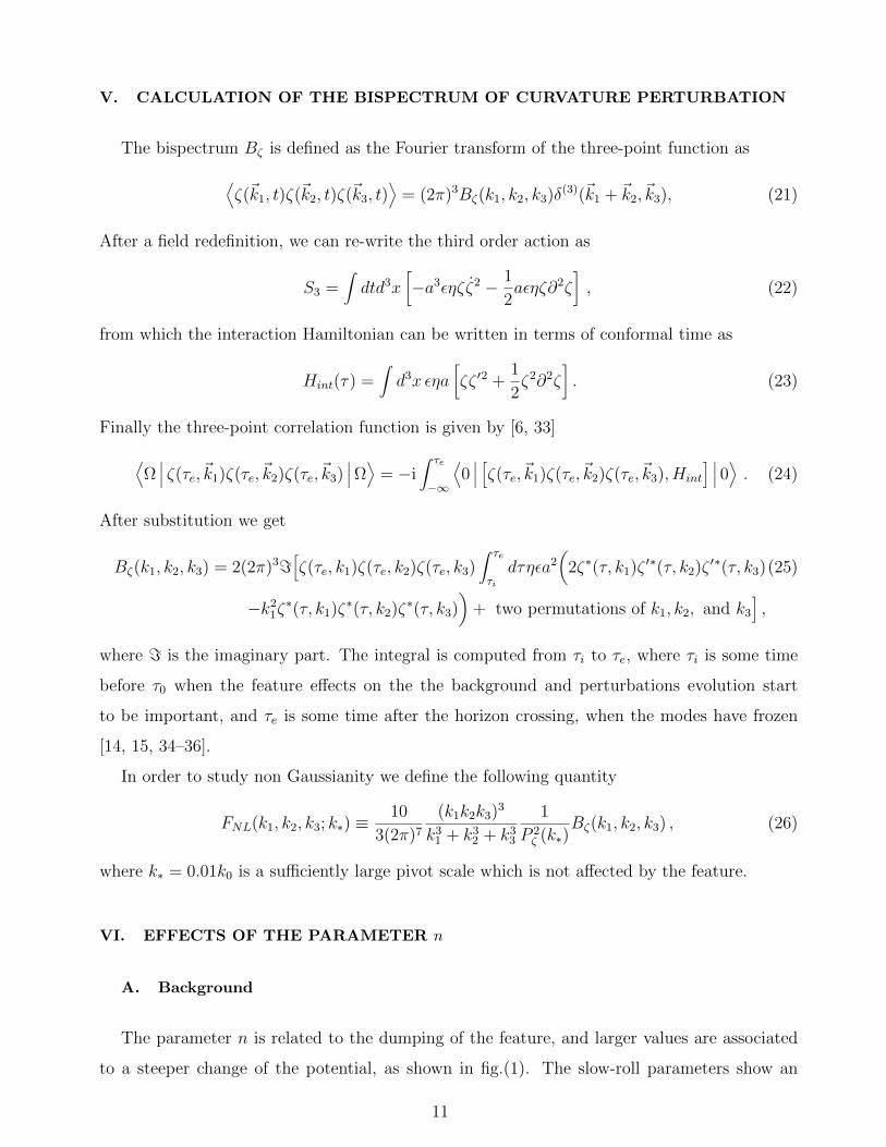
V. CALCULATION OF THE BISPECTRUM OF CURVATURE PERTURBATION
The bispectrum Bζ is defined as the Fourier transform of the three-point function as
⟨ζ(~k1, t)ζ(~k2, t)ζ(~k3, t)
⟩= (2π)3Bζ(k1, k2, k3)δ
(3)(~k1 + ~k2, ~k3), (21)
After a field redefinition, we can re-write the third order action as
S3 =∫dtd3x
[−a3εηζζ2 − 1
2aεηζ∂2ζ
], (22)
from which the interaction Hamiltonian can be written in terms of conformal time as
Hint(τ) =∫d3x εηa
[ζζ ′2 +
1
2ζ2∂2ζ
]. (23)
Finally the three-point correlation function is given by [6, 33]
⟨Ω∣∣∣ ζ(τe, ~k1)ζ(τe, ~k2)ζ(τe, ~k3)
∣∣∣Ω⟩ = −i∫ τe
−∞
⟨0∣∣∣ [ζ(τe, ~k1)ζ(τe, ~k2)ζ(τe, ~k3), Hint
] ∣∣∣ 0⟩ . (24)
After substitution we get
Bζ(k1, k2, k3) = 2(2π)3=[ζ(τe, k1)ζ(τe, k2)ζ(τe, k3)
∫ τe
τidτηεa2
(2ζ∗(τ, k1)ζ
′∗(τ, k2)ζ′∗(τ, k3)(25)
−k21ζ∗(τ, k1)ζ∗(τ, k2)ζ∗(τ, k3))
+ two permutations of k1, k2, and k3],
where = is the imaginary part. The integral is computed from τi to τe, where τi is some time
before τ0 when the feature effects on the the background and perturbations evolution start
to be important, and τe is some time after the horizon crossing, when the modes have frozen
[14, 15, 34–36].
In order to study non Gaussianity we define the following quantity
FNL(k1, k2, k3; k∗) ≡10
3(2π)7(k1k2k3)
3
k31 + k32 + k33
1
P 2ζ (k∗)
Bζ(k1, k2, k3) , (26)
where k∗ = 0.01k0 is a sufficiently large pivot scale which is not affected by the feature.
VI. EFFECTS OF THE PARAMETER n
A. Background
The parameter n is related to the dumping of the feature, and larger values are associated
to a steeper change of the potential, as shown in fig.(1). The slow-roll parameters show an
11
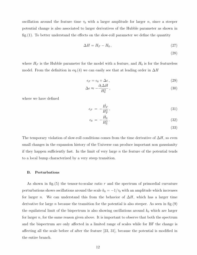
oscillation around the feature time τ0 with a larger amplitude for larger n, since a steeper
potential change is also associated to larger derivatives of the Hubble parameter as shown in
fig.(1). To better understand the effects on the slow-roll parameter we define the quantity
∆H = HF −H0 , (27)
(28)
where HF is the Hubble parameter for the model with a feature, and H0 is for the featureless
model. From the definition in eq.(4) we can easily see that at leading order in ∆H
εF = ε0 + ∆ε , (29)
∆ε ≈ −∂t∆HH2
0
, (30)
where we have defined
εF = −HF
H2F
, (31)
ε0 = − H0
H20
. (32)
(33)
The temporary violation of slow-roll conditions comes from the time derivative of ∆H, so even
small changes in the expansion history of the Universe can produce important non gaussianity
if they happen sufficiently fast. In the limit of very large n the feature of the potential tends
to a local bump characterized by a very steep transition.
B. Perturbations
As shown in fig.(5) the tensor-to-scalar ratio r and the spectrum of primordial curvature
perturbations shows oscillations around the scale k0 = −1/τ0 with an amplitude which increases
for larger n. We can understand this from the behavior of ∆H, which has a larger time
derivative for large n because the transition for the potential is also steeper. As seen in fig.(9)
the equilateral limit of the bispectrum is also showing oscillations around k0 which are larger
for larger n, for the same reason given above. It is important to observe that both the spectrum
and the bispectrum are only affected in a limited range of scales while for BF the change is
affecting all the scale before of after the feature [23, 31], because the potential is modified in
the entire branch.
12

VII. EFFECTS OF THE PARAMETER σ
A. Background
The parameters σ determines the size of the range of field values where the potential is
affected by the feature, as shown in fig.(2). The slow-roll parameters are smaller for larger σ
since a larger width of the feature tend to reduce the time derivative of the Hubble parameter
because in this case the potential modification is also associated to smaller derivatives respect
to the field due to its less steep shape.
B. Perturbations
As shown in fig.(6) the spectrum of primordial curvature perturbations and the tensor-to-
scalar ratio r have oscillations around k0, whose amplitude is larger for smaller σ, because in
this case the potential changes faster and consequently the slow-roll parameters are larger. In
fig.(10) we can see that the equilateral limit of the bispectrum also presents oscillations around
k0 with larger amplitude for smaller σ. Both for the spectrum and bispectrum the effects are
confined in a limited range of the scales, contrary to BF .
VIII. EFFECTS OF THE PARAMETER λ
A. Background
The parameter λ controls the magnitude of the potential modification, as shown in figs.(3-4).
The slow-roll parameters are larger in absolute value for larger absolute values of λ since a larger
feature of the potential induce a larger time derivative of the Hubble parameter. The sign of λ
produce opposite and symmetric effects, since it implies an opposite sign for the derivative of
the potential respect to the field, and consequently of the Hubble parameter respect to time.
B. Perturbations
As shown in fig. (7,8,12,11) larger absolute values of λ produce larger amplitude oscillations
for the tensor-to-scalar ratio r, the spectrum and bispectrum around k0. Features with the
same absolute value of λ, and opposite sign correspond to oscillations symmetric respect to the
13
featureless spectrum and bispectrum.
IX. CONCLUSIONS
We have studied the effects of of local features of the inflation potential on the spectrum
and bispectrum of single field inflationary models with a canonical kinetic term. These features
only modify the potential in a limited range of the scalar field values, and consequently only
affects the spectrum and bispectrum in a narrow range of scales which leave the horizon during
the time interval corresponding to the modification of the potential. This is different from
branch type features which effectively divide the potential into separate branches, because they
involve a step-like function in their definition, such as the Starobinsky model for example and
its generalizations. In BF models the spectrum for example exhibit a step, reminiscent of the
branch-type potential modifications, while for local features, there is no step, and the spectrum
returns to the featureless form for scales sufficiently larger or smaller than k0
The the tensor-to-scalar ratio r, the spectrum and the bispectrum of primordial curvature
perturbations are effected by the feature, showing modulated oscillations which are dumped for
scales larger or smaller than k0. The amplitude of the oscillations depends on the parameters
defining the local feature, and the effects are larger when the potential modification is steeper,
since in this case there is a stronger violation of the slow-roll conditions. Due to this local type
effect these feature could be used to model phenomenologically local glitches of the spectrum,
without affecting other scales,and it will be interesting to perform a detailed observational data
analysis in the future using the new CMB data of the Planck mission.
Acknowledgments
This work was supported by the European Union (European Social Fund, ESF) and Greek
national funds under the ARISTEIA II Action.
[1] E. Komatsu et al., (2009), arXiv:0902.4759.
[2] WMAP, G. Hinshaw et al., Astrophys.J.Suppl. 208, 19 (2013), arXiv:1212.5226.
[3] Planck Collaboration, P. Ade et al., (2013), arXiv:1303.5076.
[4] Planck Collaboration, P. Ade et al., (2015), arXiv:1502.01589.
14
[5] A. A. Starobinsky, Phys.Lett. B91, 99 (1980).
[6] J. M. Maldacena, JHEP 0305, 013 (2003), arXiv:astro-ph/0210603.
[7] Planck Collaboration, P. Ade et al., (2013), arXiv:1303.5082.
[8] Planck Collaboration, P. Ade et al., (2015), arXiv:1502.02114.
[9] Planck Collaboration, P. Ade et al., (2013), arXiv:1303.5084.
[10] Planck Collaboration, P. Ade et al., (2015), arXiv:1502.01592.
[11] A. Achcarro, J.-O. Gong, G. A. Palma, and S. P. Patil, Phys. Rev. D87, 121301 (2013),
arXiv:1211.5619.
[12] J. Martin, L. Sriramkumar, and D. K. Hazra, ArXiv e-prints (2014), arXiv:1404.6093.
[13] S. Dorn, E. Ramirez, K. E. Kunze, S. Hofmann, and T. A. Ensslin, JCAP 1406, 048 (2014),
arXiv:1403.5067.
[14] D. K. Hazra, L. Sriramkumar, and J. Martin, JCAP5, 26 (2013), arXiv:1201.0926.
[15] V. Sreenath, R. Tibrewala, and L. Sriramkumar, JCAP12, 37 (2013), arXiv:1309.7169.
[16] A. A. Starobinsky, JETP Lett. 55, 489 (1992).
[17] J. Hamann, L. Covi, A. Melchiorri, and A. Slosar, Phys.Rev. D76, 023503 (2007), arXiv:astro-
ph/0701380.
[18] D. K. Hazra, M. Aich, R. K. Jain, L. Sriramkumar, and T. Souradeep, JCAP 1010, 008 (2010),
arXiv:1005.2175.
[19] A. A. Starobinsky, Grav.Cosmol. 4, 88 (1998), arXiv:astro-ph/9811360.
[20] M. Joy, V. Sahni, and A. A. Starobinsky, Phys.Rev. D77, 023514 (2008), arXiv:0711.1585.
[21] M. Joy, A. Shafieloo, V. Sahni, and A. A. Starobinsky, JCAP 0906, 028 (2009), arXiv:0807.3334.
[22] M. J. Mortonson, C. Dvorkin, H. V. Peiris, and W. Hu, Phys.Rev. D79, 103519 (2009),
arXiv:0903.4920.
[23] A. E. Romano and A. G. Cadavid, (2014), arXiv:1404.2985.
[24] D. K. Hazra, A. Shafieloo, G. F. Smoot, and A. A. Starobinsky, Phys.Rev.Lett. 113, 071301
(2014), arXiv:1404.0360.
[25] J. A. Adams, B. Cresswell, and R. Easther, Phys.Rev. D64, 123514 (2001), arXiv:astro-
ph/0102236.
[26] A. Gallego Cadavid, Primordial non-Gaussianities produced by features in the potential of single
slow-roll inflationary models, Master’s thesis, University of Antioquia, 2013, 1330516.
[27] A. E. Romano and M. Sasaki, Phys.Rev. D78, 103522 (2008), arXiv:0809.5142.
15
[28] J. A. Adams, G. G. Ross, and S. Sarkar, Nucl.Phys. B503, 405 (1997), arXiv:hep-ph/9704286.
[29] D. Langlois, Lect.Notes Phys. 800, 1 (2010), arXiv:1001.5259.
[30] A. R. Liddle and D. Lyth, (2000).
[31] F. Arroja, A. E. Romano, and M. Sasaki, Phys.Rev. D84, 123503 (2011), arXiv:1106.5384.
[32] H. Collins, (2011), arXiv:1101.1308.
[33] X. Chen, Adv.Astron. 2010, 638979 (2010), arXiv:1002.1416.
[34] P. Adshead, C. Dvorkin, W. Hu, and E. A. Lim, Phys.Rev. D85, 023531 (2012), arXiv:1110.3050.
[35] X. Chen, R. Easther, and E. A. Lim, JCAP 0706, 023 (2007), arXiv:astro-ph/0611645.
[36] X. Chen, R. Easther, and E. A. Lim, JCAP 0804, 010 (2008), arXiv:0801.3295.
16