1

3D Solid Spherical Bispectrum CNNs forBiomedical Texture Analysis

Valentin Oreiller, Vincent Andrearczyk, Julien Fageot,John O. Prior, Senior Member, IEEE and Adrien Depeursinge, Member, IEEE

Abstract—Locally Rotation Invariant (LRI) operators haveshown great potential in biomedical texture analysis where pat-terns appear at random positions and orientations. LRI operatorscan be obtained by computing the responses to the discreterotation of local descriptors, such as Local Binary Patterns (LBP)or the Scale Invariant Feature Transform (SIFT). Other strategiesachieve this invariance using Laplacian of Gaussian or steerablewavelets for instance, preventing the introduction of samplingerrors during the discretization of the rotations. In this work,we obtain LRI operators via the local projection of the imageon the spherical harmonics basis, followed by the computationof the bispectrum, which shares and extends the invarianceproperties of the spectrum. We investigate the benefits of usingthe bispectrum over the spectrum in the design of a LRI layerembedded in a shallow Convolutional Neural Network (CNN) for3D image analysis. The performance of each design is evaluatedon two datasets and compared against a standard 3D CNN. Thefirst dataset is made of 3D volumes composed of syntheticallygenerated rotated patterns, while the second contains malignantand benign pulmonary nodules in Computed Tomography (CT)images. The results indicate that bispectrum CNNs allows for asignificantly better characterization of 3D textures than both thespectral and standard CNN. In addition, it can efficiently learnwith fewer training examples and trainable parameters whencompared to a standard convolutional layer.

Index Terms—Medical image analysis, CNN, Rotation invari-ance, Texture.

I. INTRODUCTION

CONVOLUTIONAL Neural Networks (CNNs) have re-cently gained a lot of attention as they outperform

classical handcrafted methods in almost every computer visiontasks where data scarcity is not an issue. In biomedical imageanalysis, data are abundant. However, obtaining high qualityand consistently labeled images is expensive as data curationand annotation require hours of work from well-trained experts[1]. Thus, the effective number of training examples is oftenlow. This limitation is usually handled by transfer learningand data augmentation. Transfer learning, the process of fine-tuning a network trained on another task to the task at hand,is very common for 2D images. For 3D images, however,the lack of very large datasets hinders the availability of pre-trained models. Another approach, data augmentation, refers

V. Oreiller and A. Depeursinge are with the Institute of InformationSystems, University of Applied Sciences Western Switzerland (HES-SO),Sierre, Switzerland and with the Service of Nuclear Medicine and MolecularImaging, CHUV, Lausanne, Switzerland. e-mail: valentin.oreiller@hevs.ch,adrien.depeursing@hevs.ch. V. Andrearczyk is with the Institute of Infor-mation Systems, University of Applied Sciences Western Switzerland (HES-SO), Sierre, Switzerland. J. Fageot is with Harvard School of Engineeringand Applied Sciences, Cambridge, MA, USA. J. Prior is with the Service ofNuclear Medicine and Molecular Imaging, CHUV, Lausanne, Switzerland.

to the application of geometric transforms and perturbationsto the training examples to make the CNN invariant to thesedistortions [2]. The cost of data augmentation is a substantialincrease in the data size leading to a slower convergence rateand potential waste of trainable parameters.

A lot of recent research has focused on how to build CNNsthat are invariant to these transforms by imposing constraintson the architecture of the network [3]–[6]. The motivationof these approaches is to obviate the need to learn theseinvariances from the data and their transformation. As a result,an effective reduction of the number of trainable parameters isachieved and, potentially, a reduction of the number of trainingexamples needed for the generalization of the network.

This work focuses on 3D biomedical texture analysis andon the design of CNNs that are invariant to local 3D rotations,i.e., rotations of individual local patterns. This invarianceis obtained using continuously defined Rotation Invariant(RI) descriptors of functions on the sphere. By relying ona continuous-domain formulation, we avoid the difficultiesassociated with rotations of discretized images [7], [8]. Neigh-borhoods defined by learned radial profiles are used to locallyproject the image on the solid sphere. These descriptors areused together with a convolution operation to obtain LocallyRotation Invariant (LRI)1 operators in the 3D image domainas proposed in [9]. These types of operators are relevantin biomedical texture analysis where discriminative patternsappear at random positions and orientations. The RI descrip-tors used in [5], [6], [9]–[11] and in the present work arederived from the Spherical Harmonics (SH) decomposition ofthe kernels. The SHs are the generalization of the CircularHarmonics (CH) to the 2D sphere [12]. These two familiesof functions are intimately linked with Fourier theory, andboth decompositions correspond to the Fourier transform ofthe function defined on the sphere S2 for the SHs and on thecircle S1 for the CHs.

To better apprehend the two invariants considered in thiswork, namely the spectrum and the bispectrum, it is use-ful to consider them on the circle. The CH expansion ofa function f ∈ L2(S1) for a degree n is computed asfn = 1

2π

∫ 2π

0f(θ)e−jθndθ, which is the Fourier series for

2π-periodic functions. For m,n ∈ Z, the spectrum of theCH expansion is calculated as sn(f) = fnf

∗n = |fn|2 and

the bispectrum as bn,m(f) = fnfmf∗n+m. One readily verifies

that for a function g(θ) = f(θ−θ0) we have for any m,n ∈ Z

1LRI is used for Locally Rotation Invariant and Local Rotation Invarianceinterchangeably

arX

iv:2

004.

1337

1v2

[cs

.CV

] 2

Jun

202

0

2

the equalities sn(f) = sn(g) and bn,m(f) = bn,m(g), sincegn = fne

−jθ0n. This means that the spectrum and bispectrumare RI, since a shift θ0 in the parameter of f is equivalent to arotation on the circle. The spectrum is the most simple, yet in-formative, Fourier-based RI quantity. However, it discards thephase between harmonics which contains all the informationon how the sinusoids from the expansion add up to form edgesand ridges [13, Chapter 10]. The bispectrum, on the contrary,conserves the phase information [14] and constitutes a morespecific pattern descriptor.

The main contributions of this paper are the introductionof a novel image operator based on the Solid SphericalBispectrum (SSB) that is LRI and a corresponding CNN layer,resulting in a locally rotation invariant CNN. This work buildsupon [10], where a Solid Spherical Energy (SSE) layer wasproposed. The radial profiles used to locally project the imageon the solid sphere as well as the relative importance ofthe bispectrum coefficients can be learned end to end withbackpropagation. We experimentally investigate the relevanceof the proposed SSB layer for biomedical texture classification.Finally, we study the ability of the SSB-CNN to learn withsmall amounts of data and compare with a classical CNN.

This manuscript is organized as follows. In Section II, wereview the main related works. Sections III-A to III-C describethe nomenclature and the mathematical tools used in this work.The definitions of the spectrum and bispectrum for functionsdefined on the sphere are reported in Section III-D and aredrawn from the work of Kakarala and Mao [14]. We recallthe theoretical benefits of the bispectrum over the spectrum inSection III-E. In Section III-F, we define the SSE and SSBimage operators and state that they are LRI. In Section III-G,we discuss the implementation details to integrate these imageoperators into a convolutional layer, referred to as the SSE orSSB layer. Sections IV and V detail and discuss the experi-mental evaluation of the proposed approach. Conclusions andperspectives are provided in Section VI.

II. RELATED WORK

A. Rotation Invariant Image Analysis

Combining LRI and directional sensitivity is not straight-forward and is often antagonist in simple designs [5], [15].Several methods exist to combine both properties. Ojala etal. [16] proposed the Local Binary Patterns (LBP) where theycompare values of pixels within a circular neighborhood tothe middle pixel. Pixels of the neighborhood are thresholdedbased on the central pixel to generate a binary code. LRI isachieved by ordering the binary code to obtain the smallestbinary number.

Several LRI filtering approaches were proposed. Varmaand Zisserman [17] used a filter-bank including the samefilters at different orientations, where LRI is achieved by maxpooling over the orientations. Instead of explicitly computingresponses (i.e. convolving) to oriented filters, steerable filterscan be used to improve efficiency [18], [19]. The work ofPerona [20] shows the use of steerable filters for LRI edgesand junctions analysis. Dicente et al. [21] used a filter-bankcomposed of steerable Riesz wavelets. LRI is obtained bylocally aligning the filters to the direction maximizing the

gradient of the image. Data-driven steerable filters were usedin [22] as LRI detectors of a given template within an image.Steerable Wavelet Machines (SWMs) were proposed in [23],where task-specific profiles of steerable wavelets are learnedusing support vector machines.

Other approaches have been described to obtain invariantswithout explicitly rotating the descriptors. Such methods relieson moments [24] or invariants built from the SH decom-position [25]. Kakarala and Mao introduced the bispectrumof the SH decomposition in [14] and they demonstrated thesuperiority of the bispectrum over the spectrum for 3D shapediscrimination. In [25], Kakarala showed that the bispectrumhas better properties and contains more information than thespectrum, also proving its completeness for functions definedon compact groups. More recently, an extension of the spectraland bispectral invariants was used by Zucchelli et al. [26] forthe analysis of diffusion Magnetic Resonance Imaging data.

In [6], [15], the authors used the spectrum of the SH expan-sion to compute LRI operators. Their work shares similaritieswith the method exposed here. However, our approach is moredata-driven since we learn the radial profiles, whereas they relyon handcrafted ones.

B. Rotation Equivariance in CNNs

Recently, several research contributions focused on theexplicit encoding of rotation equivariance into CNNs. Onegroup of methods relies on the extension of the classic con-volution on the group of translations to groups of symmetriesincluding rotations and reflections. A detailed description ofthe generalization of the convolution to compact groups isgiven in [27] and to homogeneous spaces in [28]. Regardingthe application of this generalization, Cohen and Welling [3]used rotations of the filters together with recombinations ofthe response maps, which is performed according to the rulesof group theory and allows equivariance to 2D right-anglerotations. The same strategy was extended to 3D imagesin [29], [30]. This 3D group CNN was applied to 3D textureclassification in [31]. Bekkers et al. [32] used the convolutionon the discretized group of 2D roto-translations. Weiler etal. [4] proposed a CH kernel representation to achieve amore efficient rotation of the filters via steerability, still in thecontext of the convolution on groups. Cohen and Welling [33]used the irreducible representation of the dihedral group tobuild CNNs that are equivariant to 2D discrete rotations.

The aforementioned methods offer the possibility to encodethe equivariance to virtually any finite group. The 2D rotationsgroup SO(2) can be uniformly discretized by choosing afinite subgroup of SO(2) with an arbitrary large numberof elements. This is not anymore the case for 3D rotationssince there is only 5 regular convex polyhedrons [34, Chapter10]. Therefore, approaches allowing for the propagation ofthe rotational equivariance without explicitly sampling thedifferent orientations are crucial in 3D. Methods involving CHand SH have been introduced to address this problem. Worrallet al. [35] used CHs representation of the kernels togetherwith a complex convolution and complex non-linearities toachieve the rotational equivariance. The main drawback isthat it generates many channels that must be disentangled

3

to achieve rotation invariance. A SH representation of thekernels was used in [11] to propagate the equivariance as ageneralization of [35] to 3D images. It is also possible to adaptneural networks to non-Euclidean domains, for instance, to the2D sphere, where the invariance to rotations plays a crucialrole as in [36] and [37]. Finally, the group convolution can beextended to more general Lie groups as proposed by Bekkersin [38], where CNNs equivariant to roto-translation and scale-translation were implemented.

Most of these methods focused on the propagation of therotation equivariance throughout the network, whereas wepropose lightweight networks discarding this information aftereach LRI layer, similarly to [5].

III. METHODS

A. Notations and Terminology

We consider 3D images as functions I ∈ L2(R3), wherethe value I(x) ∈ R corresponds to the gray level at locationx = (x1, x2, x3) ∈ R3. The set of 3D rotation matrices in theCartesian space is denoted as SO(3). The rotation of an imageI is written as I(R·), where R ∈ SO(3) is the correspondingrotation matrix.

The sphere is denoted as S2 = {x ∈ R3 : ||x||2 = 1}.Spherical coordinates are defined as (ρ, θ, φ) with radiusρ ≥ 0, elevation angle θ ∈ [0, π], and horizontal planeangle φ ∈ [0, 2π). Functions defined on the sphere arewritten as f ∈ L2(S2) and are expressed in spherical co-ordinates. The inner product for f, g ∈ L2(S2) is definedby 〈f , g〉L2(S2) =

∫ π0

∫ 2π

0f(θ, φ)g(θ, φ) sin(θ)dφdθ. With a

slight abuse of notation, the rotation of a function f ∈ L2(S2)is written as f(R·), despite the fact that spherical functionsare expressed in spherical coordinates.

The Kronecker delta δ[·] is such that δ[n] = 1 for n = 0 andδ[n] = 0 otherwise. The Kronecker product is denoted by ⊗.The triangle function is referred to as tri(x) and is defined astri(x) = 1− |x| if |x| < 1 and tri(x) = 0 otherwise. A blockdiagonal matrix formed by the sub-matrices Ai is written as[⊕

iAi]. The Hermitian transpose is denoted by †.

B. LRI Operators

This work focuses on image operators G that are LRI aspreviously introduced in [5]. An operator G is LRI if it satisfiesthe three following properties:• Locality: there exists ρ0 > 0 such that, for every x ∈ R3

and every image I ∈ L2(R3), the quantity G{I}(x) onlydepends on local image values I(y) for ‖y − x‖ ≤ ρ0.

• Global equivariance to translations: For any I ∈ L2(R3),

G{I(· − x0)} = G{I}(· − x0) for any x0 ∈ R3.

• Global equivariance to rotations: For any I ∈ L2(R3),

G{I(R0·)} = G{I}(R0·) for any R0 ∈ SO(3).

To reconcile the intuition of LRI with this definition, let usconsider a simple scenario where two images I1 and I2 arecomposed of the same small template τ ∈ L2(R3) appearingat random locations and orientations and distant enough toavoid overlaps between them. The locations of the templates

Fig. 1. Visual representation of the output of a LRI operator. Here, differentrotations are applied at the template centers. For the sake of simplicity, onlythe output values at the template centers are represented.

τ are identical for I1 and I2, the difference between the twoimages being in the local orientation of the templates. Theseimages can be written as

Ik =∑

1≤j≤J

τ(Rj,k(· − xj)),

where J is the number of occurrence of the template τ andk = 1, 2. The local orientation and position of the jth templatein image k are represented by Rj,k and xj , respectively. If theoperator G is LRI, then for any 1 ≤ j ≤ J and any rotationsRj,1, Rj,2 ∈ SO(3),

G{I1}(xj) = G{I2}(xj).From the definition of LRI, this equality is required to

hold only at the center of the templates. This example isillustrated in Fig. 1, where only the responses at the centerof the templates are represented.

In this work, the design of LRI operators is obtained in twosteps. First, the image I ∈ L2(R3) is convolved with SHsmodulated by compactly supported radial profiles, referred toas solid SHs. The second step involves the computation of RIdescriptors for each position.C. Spherical Harmonics

Any function f ∈ L2(S2) can be expanded in the form of

f(θ, φ) =

∞∑n=0

n∑m=−n

Fmn Ymn (θ, φ), (1)

where Y mn are the so-called SHs for a degree n ∈ N and orderm with −n ≤ m ≤ n. For their formal definition, see [15,Section 2.5] and for their visual representation, refer to Fig. 2.The SHs form an orthogonal basis of L2(S2) [39, Chapter 5.6].Thus, the expansion coefficients of Eq. (1) can be computedby projecting f onto the SH basis using the inner product onthe sphere

Fmn = 〈f , Y mn 〉L2(S2). (2)

This expansion corresponds to the Fourier transform on thesphere. We regroup the coefficients of all orders m for a givendegree n as the 1× (2n+ 1) vector

Fn = [F−nn . . . F 0n . . . F

nn ], (3)

4

Fig. 2. Visual representation of the real and imaginary part of theh(r)Ym

n (θ, φ) here h is chosen Gaussian for simplicity. Each box representsa given SH with the real part on the left and the imaginary part on theright. The blue represents positive values and orange negative values. Onlythe SHs for m ≥ 0 are represented since we have the following symmetryY −mn = (−1)mYm

n .

called the spherical Fourier vector of degree n. One importantproperty of SHs is their steerability, i.e. the rotation of one SHcan be determined by a linear combination of the other SHsof same degree:

Y mn (R0·) =n∑

m′=−n[Dn(R0)]m′,mY

m′

n , (4)

where Dn(R0) is a unitary matrix known as the Wigner D-matrix [39, Chapter 4]. Therefore, if two functions f, f ′ ∈L2(S2) differ only by a rotation R0 ∈ SO(3), i.e. f ′ = f(R0·),their spherical Fourier vectors, Fn and F ′n, satisfy the fol-lowing relation [14, Section 3, Eq. (5)]:

F ′n = FnDn(R0). (5)

This property is similar to the shifting property of the Fouriertransform on the real line. In the spherical case, insteadof multiplying by a complex exponential, the transform ismultiplied by the Wigner D-matrix of degree n associated withthe rotation R0.

D. Spherical RI: the Spectrum and the Bispectrum

With the properties of the spherical Fourier vectors, it ispossible to efficiently obtain RI operators for functions definedon the sphere. Two quantities computed from these coefficientswill be of interest: the spherical spectrum and the sphericalbispectrum.

1) Spectrum: The spectrum is a ubiquitous quantity insignal processing and it is well known to provide a sourceof translation invariant descriptors for periodic functions andfunctions defined on the real line. In these cases, the spectrumcorresponds to the squared modulus of the Fourier transform.Its spherical equivalent, the spherical spectrum, is defined bythe averaged squared norm of the spherical Fourier vector Fn:

sn(f) =1

2n+ 1FnF†

n =1

2n+ 1

n∑m=−n

|Fmn |2. (6)

2) Bispectrum: The bispectrum is defined as in [14, Section4 Eq. (24)]:

b`n,n′(f) = [Fn ⊗Fn′ ]Cnn′F `

†, (7)

where the term Fn ⊗Fn′ is a 1× (2n+ 1)(2n′ + 1) vector,Cnn′ is the (2n+1)(2n′+1)×(2n+1)(2n′+1) Clebsh-Gordanmatrix containing the Clebsh-Gordan coefficients, whose def-inition and main properties are recalled in Appendix A, andF ` = [0, . . . , 0,F `, 0, . . . , 0] is a zero-padded vector of size1× (2n+ 1)(2n′ + 1) containing the spherical Fourier vectorof degree ` with |n − n′| ≤ ` ≤ n + n′. The zero-padding isperformed to match the size of Cnn′ and to select only therows corresponding to the `th degree.

The spectrum and the bispectrum are known to be RI.We recall this fundamental result that will be crucial for usthereafter.

Proposition 1: The spectrum and the bispectrum of sphericalfunctions are RI. This means that, for any rotation R0 ∈ SO(3)and any function f ∈ L2(S2), we have, for f ′ = f(R0·),

sn(f) = sn(f′) and b`n,n′(f) = b`n,n′(f

′) (8)

for any n, n′ ≥ 0 and any |n− n′| ≤ ` ≤ n+ n′.

The result that the bispectrum of a spherical function isRI is given in [14, Theorem 4.1]. Besides, we introduce thefollowing notations:

S{Fn} = sn(f) (9)

andB{Fn,Fn′ ,F l} = b`n,n′(f). (10)

These notations highlight that the spectrum coefficient sn(f)only depends on the nth-order Fourier vector Fn, and thatthe bispectrum coefficient b`n,n′(f) only depends on Fn, Fn′ ,and F `. Moreover, the rotation invariance of the spectrum andbispectrum can be reformulated as

S{FnDn(R)} = S{Fn} (11)

and

B{FnDn(R),Fn′Dn′(R),F `D`(R)} = B{Fn,Fn′ ,F `}.(12)

E. Advantages of the Bispectrum over the Spectrum

Despite the simplicity to compute the spherical spectrum,it can be beneficial to use the more complete bispectrum, forwhich we provide two arguments.

1) Inter-Degree Rotations: The spectrum does not take intoaccount the inter-degree rotation. For instance, let us build afunction f ′ from the SH expansion F = (F0,F1, · · · ) ofthe function f as follows: for each degree n, we apply adifferent Wigner D-matrix Dn(Rn) with at least one rotationmatrix Rn different from the others. The corresponding SHexpansion F ′ = (F0D0(R0),F1D1(R1), · · · ) will have thesame spectrum since the Wigner D-matrices are unit matrices(i.e., they do not impact the norm of Fn).

5

2) Intra-Degree Variations: Another aspect to which thespectrum is insensitive is in the distinction of intra-degreevariations. for n0 ≥ 1 fixed, the functions f = Y mn0

havethe same spectrum sn(f) = δ[n−n0]

2n0+1 but are not rotation ofeach other in general (see Fig. 2).

On the contrary, the bispectrum does not suffer from theselimitations (see Section IV-A). Furthermore, the spectral in-formation is contained in the bispectrum. This can be easilyseen as:

bn0,n(f) = F0FnF†n = F 00 sn(f). (13)

This illustrates that, given a non-zero mean F0 = F 00 ∈ R,

we can retrieve the spectral information from the bispectrum.This can appear as a restriction for the bispectrum. However, inpractice, it is possible to add a constant to the signal ensuringthat F 0

0 is non-zero. The aforementioned properties make thebispectrum a more faithful descriptor and a good substitute ofthe spectral decomposition.

F. LRI on the Solid Sphere R3

The previous sections introduced the theoretical aspects tobuild RI descriptors for functions defined on the sphere. In thiswork, we are interested in 3D images, therefore we will usethe spherical spectrum and bispectrum in combination withsolid SHs. Solid SHs are the multiplication of the SHs by aradial profile to extend them to a 3D volume. We introducethe following notation for solid SHs evaluated on the Cartesiangrid:

κmn (x) = κmn (ρ, θ, φ) = hn(ρ)Ymn (θ, φ), (14)

where hn is a compactly supported radial profile that is sharedamong the SHs Y mn with same degree n. In the final network,the radial profiles hn are learned from the data.

The image is convolved with the solid SHs and by regroup-ing the resulting feature maps for each degree, we obtain thespherical Fourier feature maps2:

Fn(x) = [(I ∗ κmn )(x)]m=nm=−n. (15)

In other terms, the mth component of Fn(x) is〈I(x − ·), hnY mn 〉, and measures the correlation between Icentered at x and the solid SH κmn = hnY

mn . Thanks to the

Fourier feature maps, we introduce the image operators usedin this paper in Definition 1.

Definition 1: We define the SSE image operator GSSEn of

degree n ≥ 0 as

GSSEn {I}(x) = S{Fn(x)} (16)

for any I ∈ L2(R3) and x ∈ R3. Similarly, we define the SSBimage operator GSSB

n,n′,` associated with degrees n, n′ ≥ 0 and|n− n′| ≤ ` ≤ n+ n′ as

GSSBn,n′,`{I}(x) = B{Fn(x),Fn′(x),F `(x)}, (17)

2The convolution (I ∗ κmn )(x) with all the κmn is equivalent to a localprojection of the image around the position x to a function defined on thesphere followed by a projection onto the SHs basis. For that reason, we use thesame notation as for the spherical Fourier vector of degree n. We distinguishthe spherical Fourier feature maps by the evaluation over a position x.

for any I ∈ L2(R3) and x ∈ R3.

The SSE image operators have been considered in [5],where it was proven to be LRI in Appendix D. We recall thisresult and extend it to SSB image operators in the followingproposition, whose proof is given in Appendix B.

Proposition 2: The SSE and SSB image operators areglobally equivariant to translations and rotations. When theradial profiles hn are all compactly supported, these operatorsare therefore LRI in the sense of Section III-B.

G. Implementation of the LRI layers

In this section, we report the implementation details of ourLRI design.

1) Parameterization of the Radial Profiles: The radialprofiles are parameterized as a linear combination of radialfunctions

hq,n(ρ) =

J∑j=0

wq,n,jψj(ρ), (18)

where the wq,n,j are the trainable parameters of the model. In(18), hq,n is the qth radial profile associated to the degree n.The index q controls the number of output streams in the layer.The index j = 0, . . . , J controls the radial components of thefilter. The radial functions are chosen as ψj(ρ) = tri(ρ− j).

2) Number of Feature Maps: The image is convolvedwith the kernels κmq,n to obtain the spherical Fourier featuremaps {Fq,n(x)}q=1,...,Q

n=0,...,N . Here, Q is the number of outputstreams of the layer and N is the maximal degree of the SHdecomposition. These feature maps are combined according toEq. (16) and (17) resulting in GSSE

q,n {I}(x) or GSSBq,n,n′,l{I}(x)

respectively. In the following, we discuss the number of featuremaps generated for only one output stream, thus we drop theindex q.

In the case of the operator GSSEn , the number of generated

feature maps is N + 1. For the GSSBn,n′,` operator, the total

number of features maps is O(N3). It is actually not necessaryto compute all the bispectrum coefficients, some of them beingredundant due to the following properties. First, for each n,n′ and `, the bispectral components b`n,n′(f) and b`n′,n(f) areproportional independently of f [14, Theorem 4.1]. Hence,we choose to compute the components only for n ≤ n′ and0 ≤ n + n′ ≤ N . Second, even though the bispectrum iscomplex-valued, when f is real, b`n,n′(f) is either purely realor purely imaginary if n+n′+` is even or odd respectively [40,Theorem 2.2]. Thus, we can map it to a real-valued scalar.In our design, we take either the real or the imaginary partdepending on the value of the indices n, n′, `.

Even with these two properties the number of feature mapsfor the GSSB

n,n′,` operator still follows a polynomial of degree 3(see Table I for the first values), but for low N it still reducesgreatly this number. Moreover, the maximal degree N for theSH expansion cannot be taken arbitrarily large as the kernelsare discretized [5]. The upper bound for N is given by N ≤πc4 , where c is the diameter of the kernel. This condition can

be regarded as the Nyquist frequency for the SH expansion.As an example, N = 7 is the maximal value for a kernel ofsize 9× 9× 9.

6

TABLE INUMBER OF FEATURE MAPS OBTAINED FOR THE GSSE

n AND GSSBn,n′,`

OPERATORS IN FUNCTION OF THE MAXIMAL DEGREE N .

N 0 1 2 4 6 8 10 100

Spectrum 1 2 3 5 7 9 11 101Bispectrum 1 2 5 14 30 55 91 48127

3) Discretization: The kernels κmq,n = hq,nYmn are dis-

cretized by evaluating them on a Cartesian grid. For moredetails about the discretization, see [9, Section 2.4].

IV. EXPERIMENTS AND RESULTS

Section IV-A illustrates the differences between the spher-ical spectrum and bispectrum with two toy experiments de-signed to fool the spectrum. Then, we compare the clas-sification performance of three different CNNs (SSE, SSBand standard) detailed in Section IV-C on the two datasetsdescribed in Section IV-B in terms of accuracy (Section IV-D)and generalization power (Section IV-E) i.e. the number oftraining samples required to reach the final accuracy.

A. Comparing Local Spectrum to Bispectrum Representations

Two toy experiments are conducted to highlight the differ-ences in terms of the representation power of the sphericalspectrum and bispectrum. The first experiment is designedto show that the spectrum is unable to discriminate betweenpatterns that only differ in terms of rotations between degrees.The second experiment illustrates that the spectrum cannotcapture differences within the same degree. These two ex-periments are done in the 3D image domain to show theapplicability of the spherical spectrum and bispectrum of thesolid SHs and to be as close as possible to the final application.

The images are obtained by evaluatingh(ρ)

∑Nn=0

∑m=nm=−n F

mn Y

nm(θ, φ) on a 3D Cartesian grid of

32×32×32 with h defined as an isotropic Simoncelli waveletprofile [41]. This first experiment investigates the capabilityof the spectrum and bispectrum to discriminate betweenfunctions with distinct inter-degree rotations. Representativesf and f ′ of the two classes are obtained by summingthe SHs described by their repsective spherical Fouriertransform F and F ′. F is composed of F1 = [1, j, 1],F2 = [1,−1, 1, 1, 1], F3 = [1,−1, 1, j, 1, 1, 1] and Fn = 0for any n 6= 1, 2, 3. The coefficients are chosen to ensure thatthe images are real and that the spherical spectrum sn(f) = 1for n = 1, 2, 3. The spherical decomposition F ′ of the secondclass is computed as F ′1 = F1D1(R1), F ′2 = F2D2(R2)and F ′3 = F3D3(R3), where R1, R2 and R3 are distinct 3Drotations. This allows to combine the different degrees withdifferent rotations resulting in a function f ′ with spectrumsn(f

′) = sn(f) for all n but f ′ 6= f . Moreover, for eachclass, 50 distinct instances are created by adding Gaussiannoise and randomly rotating the images. The random rotationsare drawn from a uniform distribution over the 3D rotationsand then we use the associated Wigner-D matrices to rotatethe instances. This time, the same rotation is applied to alldegrees. The bispectrum and spectrum are calculated usingonly the responses to the spherical filters at the origin voxel

of the images and the results are presented in Fig. 3. Notethat only a subset of distintive coefficients of the bispectrumis shown. The results indicate that the spectrum cannot detectinter-degree rotations, whereas the bispectrum can.

s0 s1 s2 s3 s4

0

0.5

1

(a) Spectrum

b11,2 b21,2 b31,2 b21,3

−5

0

5

(b) Bispectrum

Fig. 3. Experiment with distinct inter-degree rotations. Spherical spectral(left) and bispectral (right) decomposition of the two classes. The blue barsrepresent the decomposition for the first class f and the orange bars for thesecond class f ′ (F ′i = F iDi(Ri), i = 1, 2, 3). Note that only a subset ofthe bispectral components is displayed. It can be observed that the spectrumcannot distinguish between f and f ′, and that the bispectrum can.

In the next experiment, instead of applying a distinctrotation to each degree, we choose orders that are differentwithin the same degree. For the first class f , we use onlythe order m = 0 and for the second class f ′ the ordersm = n,−n. This choice is motivated by their differences inshape as represented in Fig. 2. The spherical Fourier transformF of the first class is chosen to be F1 = [0,

√3j, 0], F2 =

[0, 0,√5, 0, 0], F3 = [0, 0, 0,

√7j, 0, 0, 0] and Fn = 0 for any

n 6= 1, 2, 3. The spherical decomposition F ′ of the secondclass is F ′1 = [

√3/2, 0,

√3/2], F ′2 = [

√5/2, 0, 0, 0,

√5/2],

F ′3 = [√7/2, 0, 0, 0, 0, 0,

√7/2]. The coefficients are chosen

to obtain a spherical spectrum of 1 for n = 1 , n = 2 andn = 3 and to generate real images. The results in Fig. 4 showthat the bispectrum can discriminate between the two classeseven though they have the same spectrum.

s0 s1 s2 s3 s4

0

0.5

1

(a) Spectrum

b21,1 b11,2 b21,2 b31,2

−5

0

5

10

(b) Bispectrum

Fig. 4. Experiment with intra-degree variations. Spherical spectral (left) andbispectral (right) decomposition of the two classes. The blue bars representthe decomposition for the first class f and the orange bars for the secondclass f ′. Note that only a subset of the bispectral components is displayed. Itcan be observed that the spectrum cannot distinguish between f and f ′, andthat the bispectrum can.

7

B. Datasets

To evaluate the performance of the proposed LRI operators,we use both a synthetic and a medical dataset. The syntheticdataset constitutes a controlled experimental setup and con-tains two classes with 500 volumes each of size 32× 32× 32for each class. They are generated by placing two types ofpatterns with a size of 7×7×7, namely a binary segment anda 2D cross with the same norm, at random 3D orientationsand random locations with possible overlap. The number ofpatterns per volume is randomly set to bd·( svsp )

3c, where sv andsp are the sizes of the volume and of the pattern, respectivelyand the density d is drawn from a uniform distribution in therange [0.1, 0.5]. The two classes vary by the proportion ofthe patterns, i.e. 30% segments with 70% crosses for the firstclass and vice versa for the second class. 800 volumes areused for training and the remaining 200 for testing. Despitethe simplicity of this dataset, some variability is introduced bythe overlapping patterns and the linear interpolation of the 3Drotations.

The second dataset is a subset of the American NationalLung Screening Trial (NLST) that was annotated by radiolo-gists at the University Hospitals of Geneva (HUG) [5]. Thedataset includes 485 pulmonary nodules from distinct patientsin CT, among which 244 benign and 241 malignant. We pador crop the input volumes (originally with sizes ranging from16×16×16 to 128×128×128) to the size 64×64×64. Weuse balanced training and test splits with 392 and 93 volumesrespectively. Examples of 2D slices of the lung nodules areillustrated in Fig. 5. The Hounsfield units are clipped in therange [−1000, 400], then normalized with zero mean and unitvariance (using the training mean and variance).

(a) Benign (b) Malignant

Fig. 5. Slices drawn from the NLST dataset showing a benign pulmonarynodule and a malignant one.

C. Network Architecture

This work uses the network architecture proposed in [9].The first layer consists of the LRI layer implemented asdescribed in Section III-G. The obtained responses are ag-gregated using spatial global average pooling, similarly to[42]. This pooling aggregates the LRI operator responsesinto a single scalar per feature map and is followed by oneFully Connected (FC) layer. For the nodule classificationexperiment, we average the responses inside the nodule masksinstead of across the entire feature maps to remove the effect ofthe size allowing the network to focus on the textural contentof the nodule. The final softmax FC layer is connected directlywith a cross-entropy loss. Standard Rectified Linear Units

(ReLU) activations are used. The two different types of LRInetworks are referred to as SSE-CNN and SSB-CNN whenthe LRI layer uses the GSSE or GSSB operator respectively.

The networks are trained using an Adam optimizer withβ1 = 0.99 and β2 = 0.9999 and a batch size of 8. Other task-specific parameters are: for the synthetic experiment (kernelsize 7 × 7 × 7, stride 1, 2 filters and 50,000 iterations), forthe nodule classification experiment (kernel size 9 × 9 × 9,stride 2, 4 filters and 10,000 iterations). The initial values ofthe trainable weights in (18) are drawn independently froma Gaussian distribution as wq,n,j ∼ N (0, 1) and the biasesare initialized to zero. This initialization is inspired by [4],[43] in order to avoid vanishing and exploding activations andgradients.

We compare the proposed CNNs to a network with the samearchitecture but with a standard 3D convolutional layer andvarying numbers of filters, referred to as Z3-CNN.

D. Classification Performance of the SSB-, SSE- and Z3-CNN

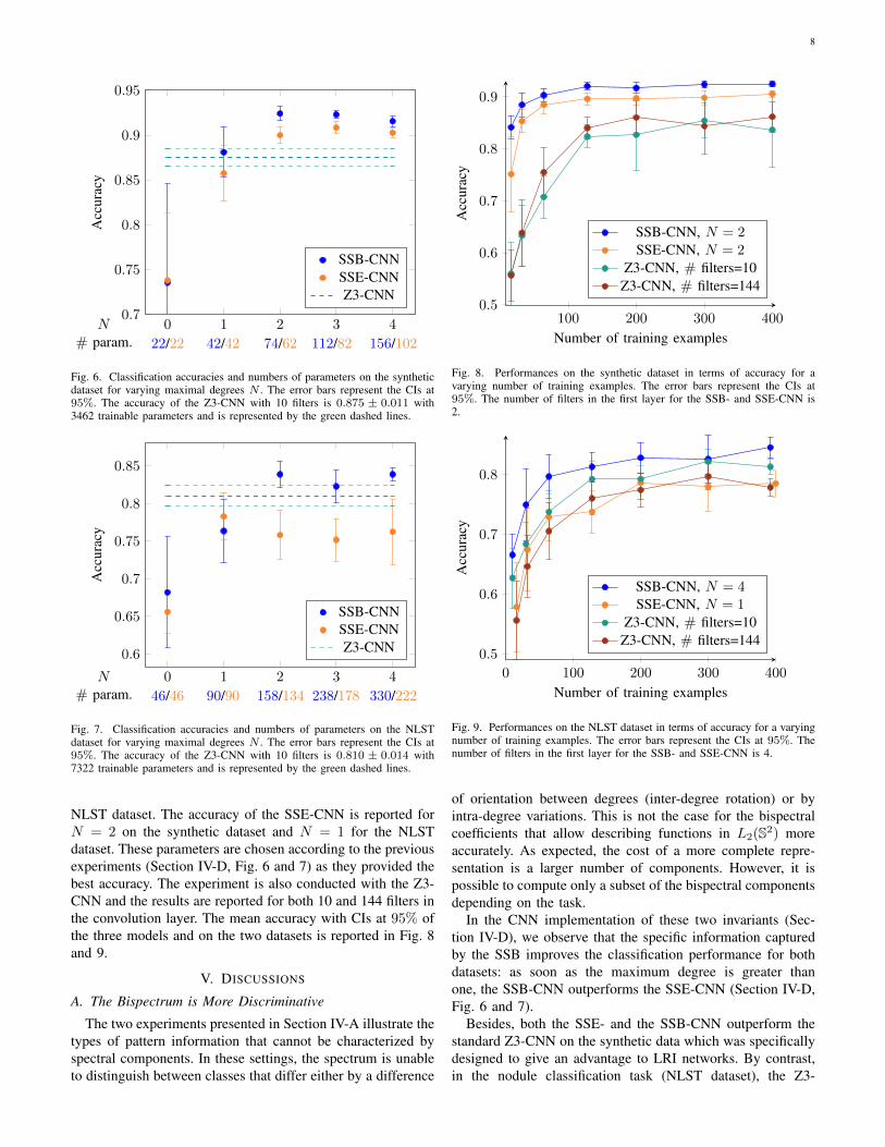
Here, we evaluate the classification performance of boththe SSE-CNN and SSB-CNN on the two datasets describedin Section IV-B. The accuracies of both designs are computedwith 10 different initializations for varying maximal degreesN . Confidence Intervals (CI) at 95% and mean accuracies arereported in Fig. 6 and 7 for the synthetic and NLST datasetsrespectively. On both datasets, the SSB-CNN outperformsthe two other networks. To exclude the possibility that thisperformance gain is simply due to a higher number of featuremaps, we trained a SSE-CNN on the synthetic dataset withmaximal degree N = 2 and 4 kernels in the first layer insteadof 2. This amounts to a total of 12 feature maps after thefirst layer. This model achieves 0.9075 ± 0.006 of accuracyand is still significantly outperformed by the SSB-CNN withmaximal degree 2 and 2 kernels, which has 10 feature mapsafter the first layer and obtains an accuracy of 0.924± 0.008(Fig. 6). One important remark is that both LRI networkscontain fewer parameters than the Z3-CNN. For instance inthe NLST experiment, the SSB- and SSE-CNN have 330 and222 parameters respectively for a maximal degree N = 4against 7322 parameters for the Z3-CNN.

E. Learning Curves of the SSB-, SSE- and Z3-CNN

The SSB- and SSE-CNN are LRI networks and thus requireneither additional training examples nor a large number ofparameters to learn this property. In addition, they rely oncompressing SH parametric representations. For these tworeasons, we expect that they will better generalize with fewertraining examples (i.e. steeper learning curve) than the stan-dard Z3-CNN on data for which this property is relevant.To test this hypothesis, we compare the classification perfor-mance of each method using an increasingly large numberof training examples Ns. For the synthetic dataset, we useNs = 16, 32, 64, 128, 200, 300, 400 and for the nodule classi-fication Ns = 10, 30, 64, 128, 200, 300, 392. For each value ofNs, 10 repetitions are made and Ns examples are randomlydrawn from the same training fold as the previous experiments(Section IV-D). For the SSB-CNN we report the accuracyfor N = 2 on the synthetic dataset and N = 4 on the

8

0 1 2 3 40.7

0.75

0.8

0.85

0.9

0.95A

ccur

acy

SSB-CNNSSE-CNNZ3-CNN

22/22 42/42 74/62 112/82 156/102N

# param.

Fig. 6. Classification accuracies and numbers of parameters on the syntheticdataset for varying maximal degrees N . The error bars represent the CIs at95%. The accuracy of the Z3-CNN with 10 filters is 0.875 ± 0.011 with3462 trainable parameters and is represented by the green dashed lines.

0 1 2 3 4

0.6

0.65

0.7

0.75

0.8

0.85

Acc

urac

y

SSB-CNNSSE-CNNZ3-CNN

46/46 90/90 158/134 238/178 330/222N

# param.

Fig. 7. Classification accuracies and numbers of parameters on the NLSTdataset for varying maximal degrees N . The error bars represent the CIs at95%. The accuracy of the Z3-CNN with 10 filters is 0.810 ± 0.014 with7322 trainable parameters and is represented by the green dashed lines.

NLST dataset. The accuracy of the SSE-CNN is reported forN = 2 on the synthetic dataset and N = 1 for the NLSTdataset. These parameters are chosen according to the previousexperiments (Section IV-D, Fig. 6 and 7) as they provided thebest accuracy. The experiment is also conducted with the Z3-CNN and the results are reported for both 10 and 144 filters inthe convolution layer. The mean accuracy with CIs at 95% ofthe three models and on the two datasets is reported in Fig. 8and 9.

V. DISCUSSIONS

A. The Bispectrum is More Discriminative

The two experiments presented in Section IV-A illustrate thetypes of pattern information that cannot be characterized byspectral components. In these settings, the spectrum is unableto distinguish between classes that differ either by a difference

100 200 300 4000.5

0.6

0.7

0.8

0.9

Number of training examples

Acc

urac

y

SSB-CNN, N = 2SSE-CNN, N = 2

Z3-CNN, # filters=10Z3-CNN, # filters=144

Fig. 8. Performances on the synthetic dataset in terms of accuracy for avarying number of training examples. The error bars represent the CIs at95%. The number of filters in the first layer for the SSB- and SSE-CNN is2.

0 100 200 300 400

0.5

0.6

0.7

0.8

Number of training examples

Acc

urac

y

SSB-CNN, N = 4SSE-CNN, N = 1

Z3-CNN, # filters=10Z3-CNN, # filters=144

Fig. 9. Performances on the NLST dataset in terms of accuracy for a varyingnumber of training examples. The error bars represent the CIs at 95%. Thenumber of filters in the first layer for the SSB- and SSE-CNN is 4.

of orientation between degrees (inter-degree rotation) or byintra-degree variations. This is not the case for the bispectralcoefficients that allow describing functions in L2(S2) moreaccurately. As expected, the cost of a more complete repre-sentation is a larger number of components. However, it ispossible to compute only a subset of the bispectral componentsdepending on the task.

In the CNN implementation of these two invariants (Sec-tion IV-D), we observe that the specific information capturedby the SSB improves the classification performance for bothdatasets: as soon as the maximum degree is greater thanone, the SSB-CNN outperforms the SSE-CNN (Section IV-D,Fig. 6 and 7).

Besides, both the SSE- and the SSB-CNN outperform thestandard Z3-CNN on the synthetic data which was specificallydesigned to give an advantage to LRI networks. By contrast,in the nodule classification task (NLST dataset), the Z3-

9

CNN outperforms the SSE-CNN. It seems that the simpledesign of the SSE-CNN fails to capture the specific signatureof malignant pulmonary nodule information on these data.However, once again, the richer invariant representation ofthe SSB-CNN allows outperforming even the Z3-CNN withstatistical significance when N = 4 while using approximately22 times fewer parameters.

B. Better Generalization of the LRI Models

The learning curve experiment on the synthetic dataset pre-sented in Section IV-E shows that both LRI designs outperformthe Z3-CNN for any number of training examples. What ismore notable is the steeper learning for the two LRI networks.Both SSE- and SSB-CNNs seem to require the same numberof training examples to reach their final performance level.For the Z3-CNN, two networks are compared: one with 10filters and the other with 144 filters, accounting for 7322 and105,410 trainable parameters, respectively. Even though thenumber of parameters is vastly different, the overall shape ofthe learning curves does not significantly change between thetwo Z3 networks, pointing out that the relationship betweennumbers of parameters and training examples is not obviousand highly depends on the architecture.

On the NLST dataset, the SSB-CNN outperforms the Z3-CNN when trained with the same number of training examples.However, the steeper learning curve of the former is lesspronounced than with the synthetic dataset. We expect the gapbetween the two learning curves to be wider if we use deeperarchitecture as the difference in the number parameters willbe higher. Overall, we observe that the proposed SSB-CNNrequires fewer training examples than the Z3-CNN, thanks toboth the LRI property and the compressing parametric SHkernel representations.

VI. CONCLUSION

We showed that, by using the highly discriminative SSB RIdescriptor, we are able to implement CNNs that are more accu-rate than the previously proposed SSE-CNN. Furthermore, wealso observed that LRI networks can learn with fewer trainingexamples than the more traditional Z3-CNN, which supportsour hypothesis that the latter tends to misspend the parameterbudget to learn data invariances and symmetries. The mainlimitation of the proposed experimental evaluation is that itrelies on shallow networks that would place these approachesmore at the crossroad between handcrafted methods and deeplearning. In future work, the LRI layers will be implementedin a deeper architecture to leverage the fewer resources thatthey require in comparison with a standard convolutional layer.This is expected to constitute a major contribution to improve3D data analysis when curated and labelled training data isscarce, which most often the case in medical image analysis.The code is available on GitHub3.

3https://github.com/voreille/ssbcnn, as of April 2020.

APPENDIX ACLEBSCH-GORDAN MATRICES

Let us fix n1, n2 ≥ 0. The Clebsch-Gordan matrix Cn1,n2

is characterized by the fact that it block-diagonalizes theKronecker product of two Wigner-D matrices as

Dn1(R)⊗Dn2

(R) = Cn1,n2

n1+n2⊕i=|n1−n2|

Di(R)

C†n1,n2(19)

for any matrix rotation R ∈ SO(3). This means in partic-ular that Cn1,n2

has∑n1+n2

n=|n1−n2|(2n + 1) rows and (2n1 +1)(2n2 + 1) columns. These two numbers are actually equal,hence Cn1,n2 ∈ R(2n1+1)(2n2+1)×(2n1+1)(2n2+1), but the re-lation (19) also reveals the structure of the matrix, whosecoefficients are indexed as Cn1,n2

[(n,m), (m1,m2)], withn ∈ {|n1 − n2|, . . . , (n1 + n2)}, m1 ∈ {−n1, . . . , n1}, andm2 ∈ {−n2, . . . , n2}. In the literature, the Clebsch-Gordancoefficients are often written with bracket notations, that revealsome of their symmetries [44]. Moreover, the Clebsch-Gordanmatrix has many 0 entries. We indeed have that

Cn1,n2 [(n,m), (m1,m2)] = 0 if m 6= m1 +m2

= 〈n1m1n2m2|n(m1 +m2)〉,

where 〈|〉 is the bracket notation used for instance in [45,Chapter 5.3.1].

APPENDIX BPROOF OF PROPOSITION 2

The equivariance to translations is simpler and similar tothe equivariance to rotations, therefore we skip it (it simplyuses that (I(·−x0)∗κmn )(x) = (I ∗κmn )(x−x0)). Let Fn(x)and F ′n(x) be the Fourier feature maps of I and I(R0·)respectively, with R0 ∈ SO(3). According to (4) applied toR = R−10 , we have that

κmn (R−10 ·) =n∑

m′=−nDn(R

−10 )m,m′κ

mn . (20)

Moreover, we have that (I(R0·) ∗ κmn )(x) = (I ∗κmn (R−10 ·))(R0x). Together with (20), this implies that

F ′n(x) = ((I(R0·) ∗ κmn )(x))m = F(R0x)Dn(R−10 x).

(21)This implies that

GSSBn,n′,`{I(R0·)}(x) = B{F ′n(x),F′n′(x),F

′`(x)}

= B{Fn(R0x)Dn(R−10 ), . . .

Fn′(R0x)Dn′(R−10 ),F `(R0x)D`(R

−10 )}

= B{Fn(R0x),Fn′(R0x),F `(R0x)}= GSSBn,n′,`{I}(R0x),

where we used the invariance of the bispectrum for the thirdequality. This demonstrates the equivariance of the operatorGSSBn,n′,` with respect to rotations. Finally, the locality simplyfollows from the fact that the convolution I ∗ κmn (x) dependson the values of I(x−y) with y in the support of κmn , whichis bounded as soon as hn is compactly supported, what weassumed.

10

ACKNOWLEDGMENT

The authors are grateful to Michael Unser, who suggestedthem to consider the bispectrum as a tool to capture rotation-invariant features of 3D signals. This work was supportedby the Swiss National Science Foundation (SNSF grants205320 179069 and P2ELP2 181759) and the Swiss Per-sonalized Health Network (SPHN IMAGINE and QA4IQIprojects), as well as a hardware grant from NVIDIA.

REFERENCES

[1] H. Greenspan, B. Van Ginneken, and R. M. Summers, “Guest editorialdeep learning in medical imaging: Overview and future promise ofan exciting new technique,” IEEE Transactions on Medical Imaging,vol. 35, no. 5, pp. 1153–1159, 2016.

[2] C. Shorten and T. Khoshgoftaar, “A survey on image data augmentationfor deep learning,” Journal of Big Data, vol. 6, no. 1, p. 60, 2019.

[3] T. Cohen and M. Welling, “Group equivariant convolutional networks,”in Proceedings of The 33rd International Conference on MachineLearning, ser. Proceedings of Machine Learning Research, M. F. Balcanand K. Q. Weinberger, Eds., vol. 48. New York, New York, USA:PMLR, 20–22 Jun 2016, pp. 2990–2999.

[4] M. Weiler, F. A. Hamprecht, and M. Storath, “Learning steerablefilters for rotation equivariant CNNs,” 2018 IEEE/CVF Conference onComputer Vision and Pattern Recognition, pp. 849–858, 2017.

[5] V. Andrearczyk, J. Fageot, V. Oreiller, X. Montet, and A. Depeursinge,“Local Rotation Invariance in 3D CNNs,” in (submitted) Medical ImageAnalysis, 2020.

[6] M. Eickenberg, G. Exarchakis, M. Hirn, and S. Mallat, “Solid harmonicwavelet scattering: Predicting quantum molecular energy from invariantdescriptors of 3D electronic densities,” in Advances in Neural Informa-tion Processing Systems, 2017, pp. 6540–6549.

[7] F. Vivaldi, “The arithmetic of discretized rotations,” in AIP ConferenceProceedings, vol. 826, no. 1. American Institute of Physics, 2006, pp.162–173.

[8] Q. Ke and Y. Li, “Is rotation a nuisance in shape recognition?” inProceedings of the IEEE Conference on Computer Vision and PatternRecognition, 2014, pp. 4146–4153.

[9] V. Andrearczyk, J. Fageot, V. Oreiller, X. Montet, and A. Depeursinge,“Exploring local rotation invariance in 3D CNNs with steerable filters,”in International Conference on Medical Imaging with Deep Learning,2019.

[10] V. Andrearczyk, V. Oreiller, J. Fageot, X. Montet, and A. Depeursinge,“Solid spherical energy (SSE) CNNs for efficient 3D medical imageanalysis,” in Irish Machine Vision and Image Processing Conference,2019.

[11] M. Weiler, M. Geiger, M. Welling, W. Boomsma, and T. S. Cohen, “3dsteerable cnns: Learning rotationally equivariant features in volumetricdata,” in Advances in Neural Information Processing Systems, 2018, pp.10 381–10 392.

[12] J. Gallier, “Notes on spherical harmonics and linear representationsof Lie groups,” http://www.cis.upenn.edu/∼cis610/sharmonics.pdf, 2009,accessed: 2020-04-13.

[13] S. W. Smith et al., The scientist and engineer’s guide to digital signalprocessing. California Technical Pub. San Diego, 1997.

[14] R. Kakarala and D. Mao, “A theory of phase-sensitive rotation invariancewith spherical harmonic and moment-based representations,” in Com-puter Vision and Pattern Recognition (CVPR), 2010 IEEE Conferenceon. IEEE, 2010, pp. 105–112.

[15] A. Depeursinge, J. Fageot, V. Andrearczyk, J. P. Ward, and M. Unser,“Rotation invariance and directional sensitivity: Spherical harmonicsversus radiomics features,” in International Workshop on MachineLearning in Medical Imaging. Springer, 2018, pp. 107–115.

[16] T. Ojala, M. Pietikainen, and T. Maenpaa, “Multiresolution gray–scaleand rotation invariant texture classification with local binary patterns,”IEEE Transactions on Pattern Analysis and Machine Intelligence,vol. 24, no. 7, pp. 971–987, July 2002.

[17] M. Varma and A. Zisserman, “A statistical approach to texture classifi-cation from single images,” International Journal of Computer Vision,vol. 62, no. 1-2, pp. 61–81, 2005.

[18] W. Freeman and E. Adelson, “The design and use of steerable filters,”IEEE Transactions on Pattern Analysis & Machine Intelligence, no. 9,pp. 891–906, 1991.

[19] M. Unser and N. Chenouard, “A unifying parametric framework for2D steerable wavelet transforms,” SIAM Journal on Imaging Sciences,vol. 6, no. 1, pp. 102–135, 2013.

[20] P. Perona, “Steerable-scalable kernels for edge detection and junctionanalysis,” in European Conference on Computer Vision. Springer, 1992,pp. 3–18.

[21] Y. Dicente Cid, H. Muller, A. Platon, P. Poletti, and A. Depeursinge, “3Dsolid texture classification using locally-oriented wavelet transforms,”IEEE Transactions on Image Processing, vol. 26, pp. 1899–1910, 2017.

[22] J. Fageot, V. Uhlmann, Z. Puspoki, B. Beck, M. Unser, and A. De-peursinge, “Principled design and implementation of steerable detec-tors,” arXiv preprint arXiv:1811.00863, 2018.

[23] A. Depeursinge, Z. Puspoki, J. P. Ward, and M. Unser, “SteerableWavelet Machines (SWM): Learning Moving Frames for Texture Clas-sification,” IEEE Transactions on Image Processing, vol. 26, no. 4, pp.1626–1636, 2017.

[24] J. Flusser, B. Zitova, and T. Suk, Moments and moment invariants inpattern recognition. John Wiley & Sons, 2009.

[25] R. Kakarala, “The bispectrum as a source of phase-sensitive invariantsfor fourier descriptors: a group-theoretic approach,” Journal of Mathe-matical Imaging and Vision, vol. 44, no. 3, pp. 341–353, 2012.

[26] M. Zucchelli, S. Deslauriers-Gauthier, and R. Deriche, “A computationalFramework for generating rotation invariant features and its applicationin diffusion MRI,” Medical Image Analysis, vol. 60, p. 101597, 2020.

[27] R. Kondor and S. Trivedi, “On the generalization of equivariance andconvolution in neural networks to the action of compact groups,” arXivpreprint arXiv:1802.03690, 2018.

[28] T. S. Cohen, M. Geiger, and M. Weiler, “A general theory of equivariantCNNs on homogeneous spaces,” in Advances in Neural InformationProcessing Systems, 2019, pp. 9142–9153.

[29] M. Winkels and T. S. Cohen, “Pulmonary nodule detection in CT scanswith equivariant CNNs,” Medical image analysis, vol. 55, pp. 15–26,2019.

[30] D. Worrall and G. Brostow, “CubeNet: Equivariance to 3D rotation andtranslation,” ECCV, Lecture Notes in Computer Science, vol. 11209, pp.585–602, 2018.

[31] V. Andrearczyk and A. Depeursinge, “Rotational 3D texture classifica-tion using group equivariant CNNs,” arXiv:1810.06889, 2018.

[32] E. J. Bekkers, M. W. Lafarge, M. Veta, K. A. Eppenhof, J. P. Pluim,and R. Duits, “Roto-translation covariant convolutional networks formedical image analysis,” in International Conference on Medical ImageComputing and Computer-Assisted Intervention. Springer, 2018, pp.440–448.

[33] T. Cohen and M. Welling, “Steerable CNNs,” arXiv:1612.08498, 2016.[34] H. S. M. Coxeter, Introduction to geometry. New York, London, 1961.[35] D. E. Worrall, S. J. Garbin, D. Turmukhambetov, and G. J. Brostow,

“Harmonic networks: Deep translation and rotation equivariance,” 2017IEEE Conference on Computer Vision and Pattern Recognition (CVPR),pp. 7168–7177, 2016.

[36] R. Kondor, Z. Lin, and S. Trivedi, “Clebsch-Gordan nets: a fully Fourierspace spherical convolutional neural network,” in Advances in NeuralInformation Processing Systems, 2018, pp. 10 117–10 126.

[37] T. Cohen, M. Geiger, J. Kohler, and M. Welling, “Spherical CNNs,”arXiv preprint arXiv:1801.10130, 2018.

[38] E. J. Bekkers, “B-Spline CNNs on Lie groups,” arXiv preprintarXiv:1909.12057, 2019.

[39] D. Varshalovich, A. Moskalev, and V. Khersonskii, Quantum theory ofangular momentum. World Scientific, 1988.

[40] R. Kakarala, P. Kaliamoorthi, and W. Li, “Viewpoint invariants fromthree-dimensional data: the role of reflection in human activity under-standing,” in CVPR 2011 WORKSHOPS. IEEE, 2011, pp. 57–62.

[41] J. Portilla and E. P. Simoncelli, “A parametric texture model based onjoint statistics of complex wavelet coefficients,” International journal ofcomputer vision, vol. 40, no. 1, pp. 49–70, 2000.

[42] V. Andrearczyk and P. Whelan, “Using filter banks in convolutionalneural networks for texture classification,” Pattern Recognition Letters,vol. 84, pp. 63–69, 2016.

[43] K. He, X. Zhang, S. Ren, and J. Sun, “Delving deep into rectifiers:Surpassing human-level performance on imagenet classification,” inProceedings of the IEEE international conference on computer vision,2015, pp. 1026–1034.

[44] A. Alex, M. Kalus, A. Huckleberry, and J. von Delft, “A numericalalgorithm for the explicit calculation of su(n) and sl(n, c) Clebsch–Gordan coefficients,” Journal of Mathematical Physics, vol. 52, no. 2,p. 023507, 2011.

[45] M. Chaichian and R. Hagedorn, Symmetries in quantum mechanics: fromangular momentum to supersymmetry, 1st ed. CRC Press, 1998.