Purdue UniversityPurdue e-Pubs

ECE Technical Reports Electrical and Computer Engineering

7-1-1996

Effect of Value Based Software Engineering onDevelopment ProjectsRaymond PaulPentagon

Mageda A. SharafeddinPurdue University School of Electrical and Computer Engineering

Y. ShinagawaUniversity of Tokyo, Deptment of Information Science

Arif GhafoorPurdue University School of Electrical and Computer Engineering

Follow this and additional works at: http://docs.lib.purdue.edu/ecetr

This document has been made available through Purdue e-Pubs, a service of the Purdue University Libraries. Please contact epubs@purdue.edu foradditional information.

Paul, Raymond; Sharafeddin, Mageda A.; Shinagawa, Y.; and Ghafoor, Arif, "Effect of Value Based Software Engineering onDevelopment Projects" (1996). ECE Technical Reports. Paper 97.http://docs.lib.purdue.edu/ecetr/97

TR-ECE 96-1 1 JULY 1996

Effect of Value Based Software Engineering on Development Projects

Raymond Paul 3000 Defense Pentagon

Room 3D 1080 Washington, DC 20230

Mageda A. Sharafeddin 1285 EE Building

School of Electrical and Computer Engineering Purdue University

W. Lafayette, IN 47907-1285

Y. Shinagawa Dept. of Information Science,

University of Tokyo, Tokyo, Japan

Arif Ghafoor 1285 EE Building

School of Electrical and Computer Engineering Purdue University

W. Lafayette, IN 47907-1285

Abstract:

Previous models of software development projects have failed to represent people

productivity accurately. In this paper, we present a model characterized by realistic

productivity curves and flexibility in choosing resource factors in a software engineering

project. A two-mode mathematical model similar to PutnamNorden model js presented.

The proposed model enhances the capability of engineering management users to make

corrective actions when appropriate. It is extremely beneficial to detect problems and

provide corrective actions since they are in many cases crucial to the successful project

software engineering hiring and/or acquisition management planning to use the software

product.

1 Introduction

Software development models provide techniques for estimating schedule, total

cost, and total manpower or labor. The estimation should be as realistic as possible to

real life situations. Productivity, although defined differently by software engineers, is

considered an important attribute in a software development project. Norden[3] defines a

development project as a finite sequence of purposeful, temporally ordered activities,

operating on a homogenous set of problem elements, to meet a specified set of objectives

representing an increment of a technological advance." If we consider each new software

system as a technological advance, then the people or team members play a major role in

this advancement.

In a cost model proposed in [7], cost is directly proportional to productivity and

project engineering software system. Productivity can be based on a number of factors

such as the effectiveness of software development CASE tools, change in the stability of

specification and the frequency of such change, design configuration stability, and quality

requirements. Productivity, as defined in [7], can be improved by the softwisre

management team who can select factors to improve productivity. Productivity as

defined in [9] can be viewed as a function of future concerns such as remaining tasks to

be captured or the and remaining project time.

In a study about predicting software productivity [lo], it is indicated that

companies measure software development by the line of code developed by programmers.

The study suggests that coding is only a part of many activities that a software

development engineer has to perform such as attending meetings, taking courses, and

1

calling out detailed planning. An experimental approach is instead proposed. Based on

pre-existing productivity data recorded about a specific programmer or team, predictions

can be made about the same programmer or team. It has been noted in [8] that during the

life cycle of a project, the productivity of team members increases progressively. Such

productivity can be the result of formal experience or increased learning capability.

Human productivity as a result is the increasing capability to solve conformity and

complexity problems. All these definitions of productivity can be transformed into the

notion of quality, since all such factors effect the ultimate quality of the product.

There have been different practical and theoretical paradigms in devt:loping

software systems. To minimize delivery time, some companies use software analyzers

during the coding phase. The purpose is to detect interface errors which contribute to

about 75% of all errors in a system. These errors are found in the testing phase of

traditional systems. Furthermore, in some software environments additionall 10% errors

are detected by test cases which are automatically generated by special software testing

tools. By automatically detecting up to 85% of all the errors in a software system,

delivery time can be reduced. In this regard, computer-aided software engineering

(CASE) tools can help in increasing productivity and reducing errors as well and hence

improving the quality. Theoretical estimation models, on the other hand, arle categorized

into two main categories: static and dynamic. Static models take a unique variable, such

as size, as a starting point and uses that variable to calculate other variables such as the

cost. In dynamic models, on the other hand, variables are inter-dependent; no basic

variable is used. Two well-known models each fall into one of these two categories: The

COCOMO model, which is a static model, and PutnarnlNorden, which is a dynamic

model.

2 Background in Cost Estimation Models

An estimation model is defined as a scheme that predicts computer software data required

by project planning steps using empirically derived formulae. Due to limited number of

samples that provide empirical data, no estimation model can be used for all types of

software and development environments. Therefore, estimation models must be used

cautiously.

Static models can be further divided into two groups: single-variable and multivariable.

Single-variable methods make use of a single basic variable to estimate other desired

values. A typical equation that formulates this type of models is:

C = ash

where C is the cost and S is the size of the code and a and b are constants.

Static, multivariable models are generally based on the same principle, except that the

parameters depend on more than one variable such as methods used, user participation,

memory constraints etc. Among the numerous models in the literature which fall into this

category, COCOMO is the most widely accepted model which is elaborated in the next

section.

The COCOMO model, abbreviated for the Constructive Cost Model (COCC)MO), is a

hierarchy of software estimation models [ 1. This hierarchy consists of three sub-models,

illustrated below:

Basic Sub-Model: This is a static single-valued model that relates the effort ((cost) of the

software development to the size of the code.

Intemediate Sub-Model: This sub-model uses a set of "cost drivers" in addition to

program size to compute the cost of the projects.

Advanced Sub-Model: This sub-model takes the effect of cost drivers on each

development step of the development process into account.

The basic COCOMO model is used for quick and efficient estimation in most of the

small- to medium-sized software projects. Three modes of software development are

considered in this model, namely: the organic mode, the embedded mode, and the semi-

detached mode. The organic mode deals with simple projects in which a team of

experienced programmers work in small groups. In embedded mode, a project is assumed

to have tight hardware, software, and operational constraints. The semi-detached mode is

an intermediate mode between the organic mode and embedded mode. The mathematical

models for determining the manpower, cost, and the development time for the organic,

semi-detached and embedded modes, respectively, are as follows:

These models provide an estimate for the approximate development time in terms of the

cost and the projected program size. We use the relationship between the completion time

and cost to determine the performance profile of projects for different cost levels. The

same is done for varying manpower levels (team sizes), using a dynamic estimation

model which is discussed next.

3 The PutnarnNorden Model

The objective of this model is to progressively reduce the number of problems (tasks) or

faults in a project at a constant rate and hence model productivity as a linear learning

curve [4]. The following assumptions are made in this model:

1. The number of problems to be solved is unknown a prior but finite.

2. The problem-solving effort does make an impact on the unsolved problem set.

3. A decision removes one unsolved problem from the set.

4. The staff size is proportional to the number of problems seeking solution.

The above assumptions lead to a Rayleigh distribution of manpower over th12 course of

project development. This is due to the assumption that the number of problems to be

solved is unknown and finite, and the total manpower effort, K, is an indicator of the

number of problems. The rate of variation for the cumulative manpower cost, dC, dt

signifies the number of people involved in the project, m(t). The cumulative cost C(t) can

then be expressed as:

According to the fourth assumption given above, the number of people involved is

proportional to the effort remaining to be employed. Therefore,

where K is the total manpower effort and p(t) is a proportionality factor, which is a

function of time and it takes the effect of learning/productivity into account. By

integrating this equation, one obtains:

Another assumption that is made in this model is that the most representative learning

curve is linear. This linearity is expressed as:

p(t) = 2at

where a is a positive constant number. By carrying out the integration in Equation 2, one

obtains the expression of the cumulative manpower cost as:

C(t) = K [ I - exp(-at 2 ) ] (3)

The manning of the project can easily be obtained by differentiating the above equation:

m(t) = 2 at exp(-at ) (4)

which represents a Rayleigh distribution. m(t) is zero at the beginning of the project, has a

single peak at a time value which is a function of the constant a and then asymptotically

decreases towards zero. By deriving the function m(t) and finding its zero point, i.e., the

peak time, we can find the so called, development time, which is given below:

By substituting the values of td intothe cumulative cost equation (3), the cost at t , can be

found in terms of the total effort spent, K :

This representation, which has frequently been verified in industry on large-scale project

developments involving high technology has an important implication. It allows us to

carry out the scalability of the software development profile, which according to

Putnarnmorden model, states that the completion of intermediate software problems must

be proportional to the completion of the entire project. For example, if the project is to be

completed in half the time, all steps have to be done so. This is due to the fact that the

time variable t appears in the cost equation in a simple form and can be easily proven.

The COCOMO model has its limitations as it does not allow factors to be

introduced other than those given in the model. This model considers variations other

than those caused by the specified factors of this model to be errors [7]. An extension to

the COCOMO model has been proposed in [7]. The extension allows users to select

factors according to actual data. A data set of software metrics collected from 7 1

software development projects has been used to derive the cost model. Statistical

techniques such as regression analysis and principal component analysis is the basis of

this extension. The fact that users can select factors is advantageous, although the

representation means of these factors are limited. Team ability, for example, is

represented as a set of four values (-2, -1, +1, and +2) where -2 represents the lowest

ability level while +2 is for the highest level.

In order to provide a more comprehensive model we need a representation that is

time changing or temporal. The reason is that in reality, changing team sizes, mobility of

developers, and changing CASE technology have significant impact on the development

of a software product and the time-changing parameter must be captured in a succinct

manner. Although the PutnamDJorden model deals with a time varying procluctivity or

learning capability, its modeling of human productivity doesn't represent re,al life

situations. For example according to this model during the life cycle of a project, team

members acquire more and more knowledge about the problems of the project.

Productivity or capability to solve problems continues to increase indefinitely. There are

two reasons that invalidate the linear productivity rate:

The learning process of human beings about a specific problem tend to saturate.

Problems in a development software project are finite.

The level of full-time-equivalent software personnel active on a project tends to

follow a continuous curve where the instantaneous full-time commitment of a large

number of people is an unlikely event [6]. As mentioned above, the model suggested in

[6] indicates that the labor or manpower distribution for a number of software projects

can be approximated by the Rayleigh distribution. From this distribution various

important parameters can be obtained including the development time of a project, the

peak manpower required, and the project finishing time. The development time, as

mentioned in [ 1, is the time at which peak manpower occurs. It is the delivery time

before which effort is spent on specification, design, coding, testing, and q~~alification [6].

Manpower requirements drop after the delivery time since the most of effori. from that

point on is spent on maintenance and modifications. At the delivery time, the product is

considered operational [4,5]. It has frequently been verified in industry on large-scale

project developments involving high technology that 39 percent of a software

development project cost is consumed by the delivery time.

In this report we propose a model that combines the flexibility of model proposed

in [7] and a more realistic time changing productivity model. In our model we consider

two cases about the learning or productivity in a software development project. These

includes:

a rapid learninglproductivity model

an average learninglproductivity model

The objective of our new models is not only to accurately analyze the man power

and cost entities but also help us in improving the decision making process by providing

9

corrective alternatives. In order to facilitate this process we need to develop a powerful

estimation mechanism that is as realistic as possible for the life cycle of a project,

accurately predicts the maximum manpower required, and the time at which the

maximum manpower occur. By proposing such a technique, we can find answers to

some critical management issues such as:

How to meet the completion deadline by choosing appropriate team members.

Whether or not the current team satisfies the desired time requirements or not at any

time in the project life.

How to make corrective actions at any point of the project due to changes in time

requirements or quality of the project.

How to predict the cost and quality based on the present and the past dat.a.

Corrective actions may imply replacing old team by a more advancedlskilled personnel,

or bringing few expert software developers into the process. The proposed rnodel is not

limited to the productivity aspects of the development team. To some extent:, it can also

be used to study the effect of evolving CASE technology on the development process of

the software project. It also implies changing cost assignments to control tht: quality of

the project.

We apply our analysis to three major software metrics, namely, design stability, fault

profiles, and requirement stability data and discuss our result at the end of the report.

4 The Proposed Models for Metric-Based Decision/Quality Tradeoffs

As mentioned earlier, we propose two new models for estimating the impaclt of team

productivity and, in general, the impact of software environment such as the. use of CASE

technology on the cost and quality of project. Specifically, we illustrate the effects of

varying team size and costs on the progress of software projects. We use the following

three software metrics for the measurement of the progress. The following nnetrics

identify the quality of project:

Design Stability.

Fault Profiles

Requirement Stability

4.1 The Rapid Learning Model:

In the rapid learning model, productivity is assumed to grow exponentially. In

other words, the model emphasizes the fact that during the life cycle of a project, team

members' capability to solve problems increase exponentially until a final saturation

level. When this final level is reached, team's productivity is maintained. Following are

the reasons for choosing such model:

1. The saturation of the learning process indicates that the team cannot conltinue to

acquire knowledge about the project indefinitely.

2. Since productivity represents the ability of solving problems, and because problems

are resolved with the passage of time and thus decrease in number; productivity also

decreases with time.

11

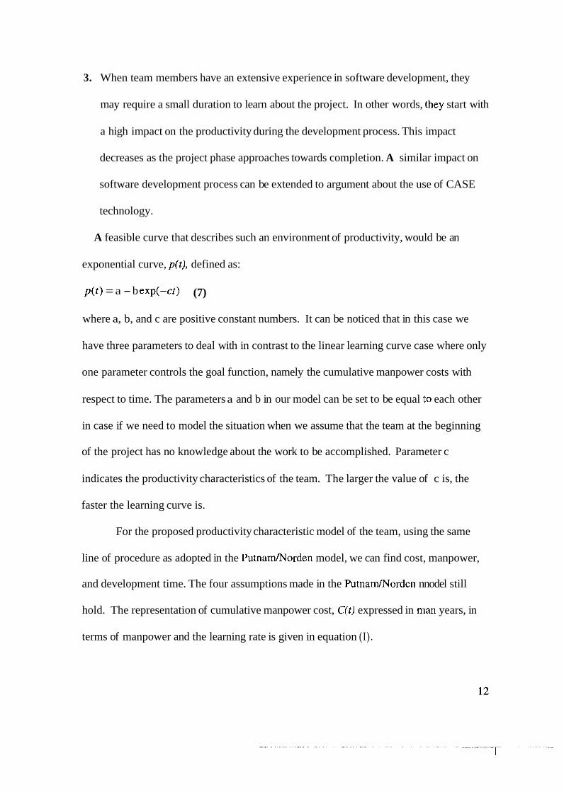
3. When team members have an extensive experience in software development, they

may require a small duration to learn about the project. In other words, Ithey start with

a high impact on the productivity during the development process. This impact

decreases as the project phase approaches towards completion. A similar impact on

software development process can be extended to argument about the use of CASE

technology.

A feasible curve that describes such an environment of productivity, would be an

exponential curve, p(t), defined as:

p(t) = a - b exp(-ct) (7)

where a, b, and c are positive constant numbers. It can be noticed that in this case we

have three parameters to deal with in contrast to the linear learning curve case where only

one parameter controls the goal function, namely the cumulative manpower costs with

respect to time. The parameters a and b in our model can be set to be equal to each other

in case if we need to model the situation when we assume that the team at the beginning

of the project has no knowledge about the work to be accomplished. Parameter c

indicates the productivity characteristics of the team. The larger the value of c is, the

faster the learning curve is.

For the proposed productivity characteristic model of the team, using the same

line of procedure as adopted in the Putnam/Norden model, we can find cost, manpower,

and development time. The four assumptions made in the Putnam/Norden nnodel still

hold. The representation of cumulative manpower cost, C(t) expressed in man years, in

terms of manpower and the learning rate is given in equation (I) .

It is worthwhile to mention that the cumulative manpower cost effort, C(t),

is null at the beginning of the project and grows towards the total effort, K. Using the

new model (equation 7) with equation (I) and carrying out the integration we find the

cumulative manpower cost as follows:

(8)

In this case the manning of the project would be:

a m(t) = ~ a ( 1 - exp(-ct)) x exp

(9)

As mentioned earlier, m(t) is zero at the beginning of the project (when t = O), and

it has a single peak at the time, whose value depends on the constants a and c. m(t) then

asymptotically decreases towards zero. Deriving m(t) and finding its zero point, we get a

quadratic equation of the form:

a' exp(-2ct) - (2a2 + ac) x exp(-ct) + a 2 = 0

The solutions to this equation, each representing the peak time whiclh is referred to

as the development time, are obtained as:

(10)

By substituting these values of td into equation (8), the cumulative clost in terms

of the total effort spent, K, can be given as:

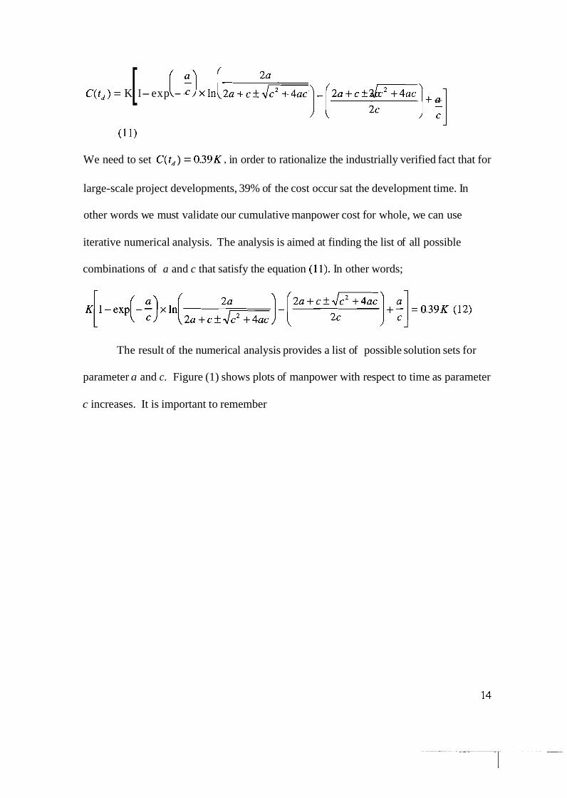
2a ~ ( t , ) = K [ I-exp ( -- :) xln ( 2 a + c , . \ I G ] - [ 2 a + c i " 4 - ] 2c

-I- - :] (1 1)

We need to set C(t, ) = 0.39K, in order to rationalize the industrially verified fact that for

large-scale project developments, 39% of the cost occur sat the development time. In

other words we must validate our cumulative manpower cost for whole, we can use

iterative numerical analysis. The analysis is aimed at finding the list of all possible

combinations of a and c that satisfy the equation (1 1). In other words;

The result of the numerical analysis provides a list of possible solution sets for

parameter a and c. Figure (1) shows plots of manpower with respect to time as parameter

c increases. It is important to remember

man power

16 1 I I I I I I I I

time

Figure (1) Rayleigh Distribution on manpower

that the total manpower effort, K, is assumed to be constant. It can be observed from this

figure that c affects the overall distribution of manpower over time. It affects the

development time as well as the peak manpower at development time. For example, for

c=0.1 (a=b=5) the development time is as high as 1.5 years while the maxiinurn required

team size is 4 persons. For the other extreme case, among the ones showed in the figure,

when c = 1.9 (a=b=5) the development time is as low as 0.3 years while the maximum

manpower required is 15 persons. Notice that the assumption that K is constant justifies

the reason that the peak manpower increases with an increase in the learning rate c. This

might not seem intuitive, because we can think that the same peak team size, i.e.;

constant peak manpower, can reduce the development time when the team members are

15

more productive resulting in a large volume of c. The assumption that K is constant

requires a constant area under each manpower curve, which when changing c changes

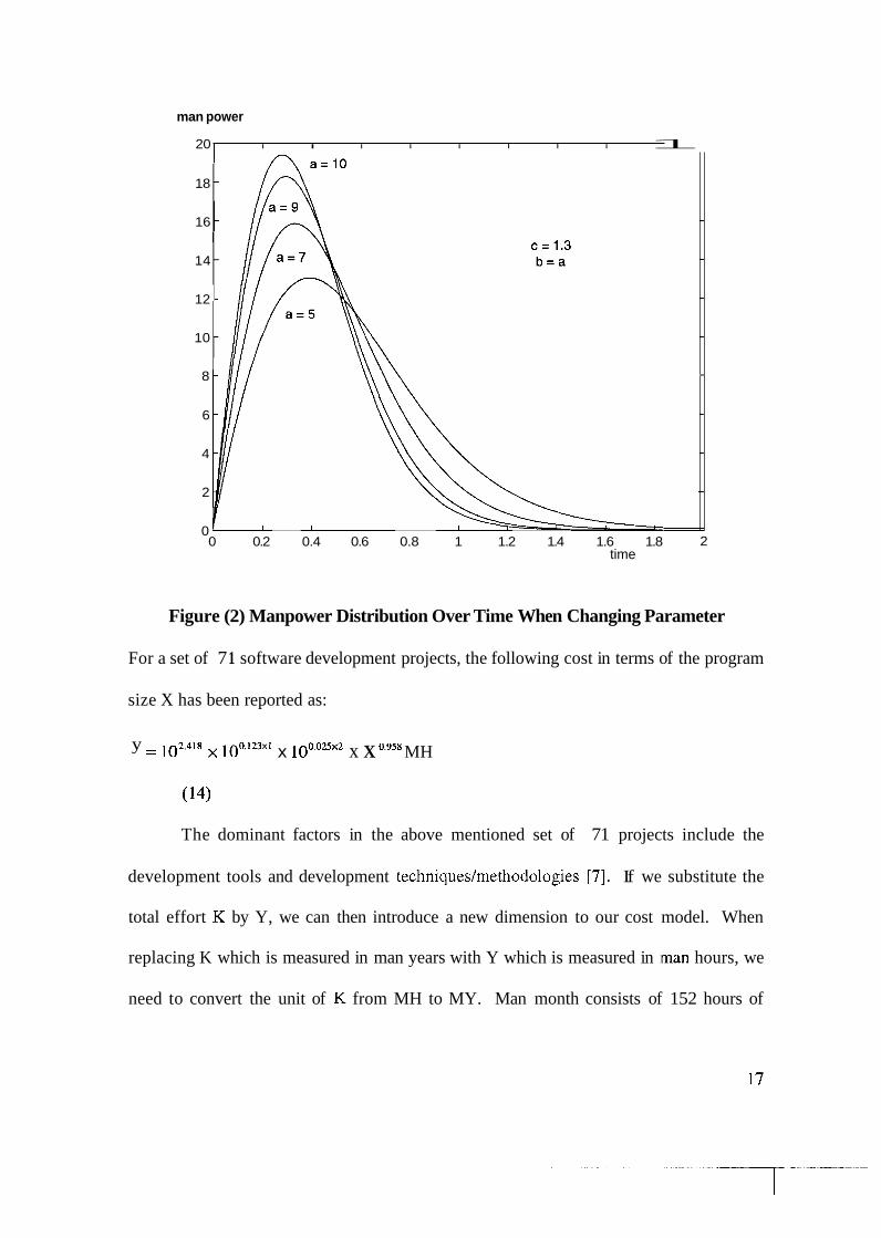
both the peak manpower and the development time. Figure (2) shows that changing a,

while keeping c constant, has little impact on the development time and has a more

obvious impact on the maximum manpower required.

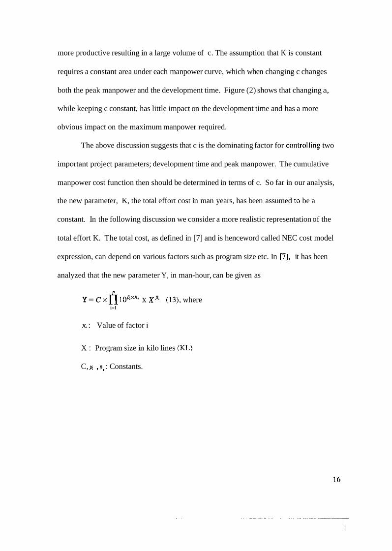
The above discussion suggests that c is the dominating factor for coritrolling two

important project parameters; development time and peak manpower. The cumulative

manpower cost function then should be determined in terms of c. So far in our analysis,

the new parameter, K, the total effort cost in man years, has been assumed t:o be a

constant. In the following discussion we consider a more realistic representation of the

total effort K. The total cost, as defined in [7] and is henceword called NEC cost model

expression, can depend on various factors such as program size etc. In [7], it has been

analyzed that the new parameter Y, in man-hour, can be given as

P

Y = c x n l ~ ~ ; ~ ~ ~ x xp5 (13), where i=l

xi : Value of factor i

X : Program size in kilo lines (KL)

C, pi , p, : Constants.

man power

20 1 I I I I I I I I 1

Figure (2) Manpower Distribution Over Time When Changing Parameter

For a set of 7 1 software development projects, the following cost in terms of the program

size X has been reported as:

y = 102.418 100.123~1 x x X 0.958 MH

(14)

The dominant factors in the above mentioned set of 71 projects include the

development tools and development techniques/methodologies [7]. If we substitute the

total effort K by Y, we can then introduce a new dimension to our cost model. When

replacing K which is measured in man years with Y which is measured in .man hours, we

need to convert the unit of K from MH to MY. Man month consists of 152 hours of

18

16

14

12

10

8

6

4

2

0 0 0.2 0.4 0.6 0.8 1 1.2 1.4 1.6 1.8

-

-

-

-

-

-

-

-

2 time

working time[6] which means that a man year is 1824 man hours. For the rapid learning

model the extended cost expression is thus defined as:

(15)

As discussed before we set a = b, and

(1 7)

It is important to indicate that the development time is not changed, and remains as:

2a t, = -1n

2a +c+ J G

The expression (16) and. (17) provide analytical estimations for the cost and the

manpower required, both as a function of program size and the effectiveness of software

tool and team over a period of time.

4.2 The Effect of Rapid Productivity on the Quality

One of our research objectives is to determine how the change in va:rious

parameters such as cost, time, and productivity (tearn1CASE technique) can affect the

quality of an ongoing development of a software product. For such purpose., we can use

the four software metrics mentioned above, namely; requirement stability, fault profile,

18

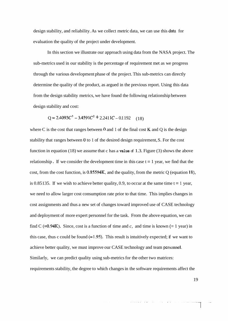
design stability, and reliability. As we collect metric data, we can use this data for

evaluation the quality of the project under development.

In this section we illustrate our approach using data from the NASA project. The

sub-metrics used in our stability is the percentage of requirement met as we progress

through the various development phase of the project. This sub-metrics can directly

determine the quality of the product, as argued in the previous report. Using this data

from the design stability metrics, we have found the following relationship between

design stability and cost:

Q = 2.4093C3 - 3.4591C2 + 2.241 lC - 0.1 192 (18)

where C is the cost that ranges between 0 and 1 of the final cost K and Q is the design

stability that ranges between 0 to 1 of the desired design requirement, S. For the cost

function in equation (18) we assume that c has a value of 1.3. Figure (3) shows the above

relationship . If we consider the development time in this case t = 1 year, we find that the

cost, from the cost function, is 0.85594K, and the quality, from the metric Q (equation 18),

is 0.85 135. If we wish to achieve better quality, 0.9, to occur at the same time t = 1 year,

we need to allow larger cost consumption rate prior to that time. This implies changes in

cost assignments and thus a new set of changes toward improved use of CASE technology

and deployment of more expert personnel for the task. From the above equation, we can

find C (=0.94K). Since, cost is a function of time and c, and time is known (= 1 year) in

this case, thus c could be found (=1.95). This result is intuitively expected; if we want to

achieve better quality, we must improve our CASE technology and team perslonnel.

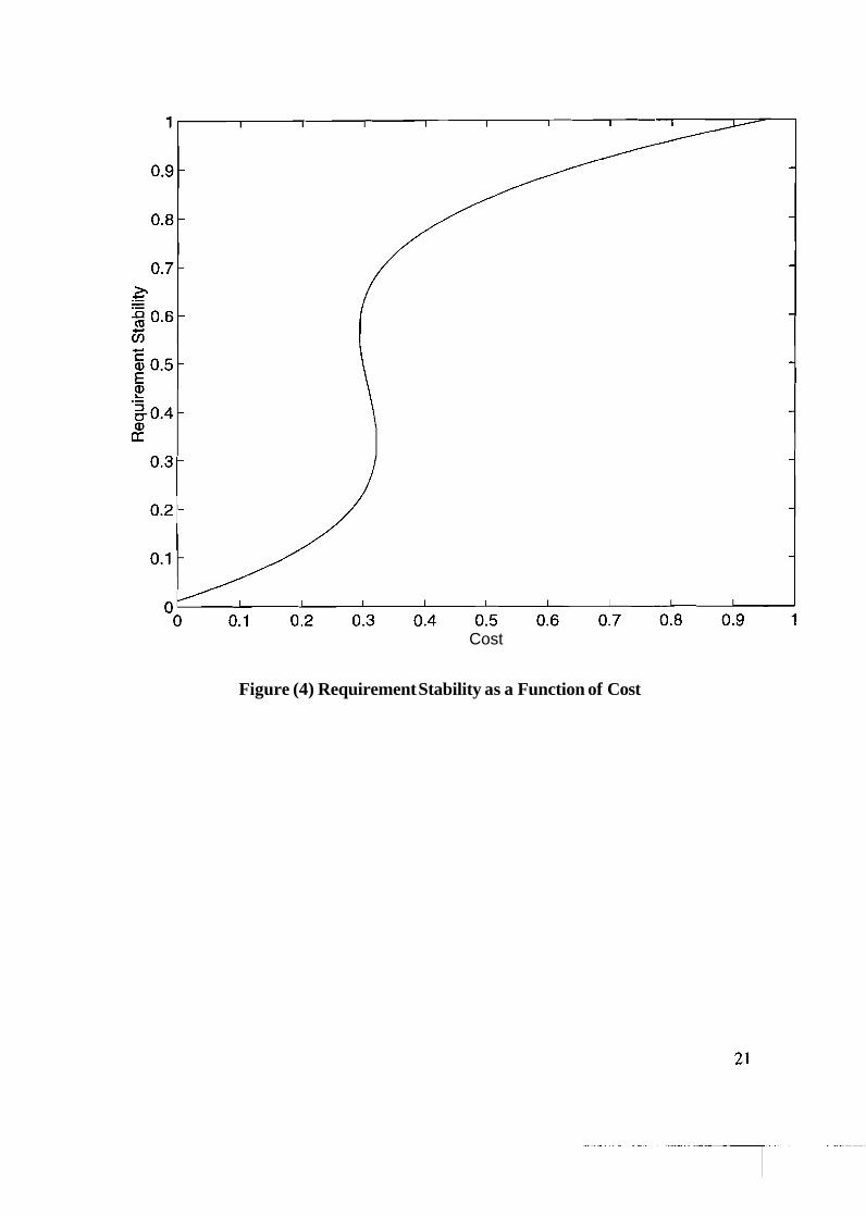
Similarly, we can predict quality using sub-metrics for the other two matrices:

requirements stability, the degree to which changes in the software requirements affect the

19

development effort; and fault profile, the number of known faults fixed. Using the NASA

data, we have found the following relation between the requirements stability (R), and fault

profile (F) in terms the cost, C .

R = 1000(4.5529C3 - 6.1759~' + 2.6081C - 0.0305) (19)

F = 1000(2.2699C3 - 3.1848~' + 1.4565C- 0.0401) (20)

Cost

Figure (3) Quality as a Function of Cost

These relations have been plotted in Figure 4 and 5.

Cost

Figure (4) Requirement Stability as a Function of Cost

0 I I I I I I I

0 0.1 0.2 0.3 0.4 0.5 0.6 0.7 0.8 0.9 1 Cost

Figure (5) Fault Profile as a Function of Cost

4.3 Average Productivity Model

In this section we introduce the second model to represent an environment that

represents the average effectiveness of CASE technology and performance of personnel.

In this model, the productivity is assumed to be considerably slow in the beginning of the

development process. After a slow start-up, the team members become more productive

and their effectiveness starts following the rapid productivity curve discussed in the

previous section. Such a model is quite common because it represents the following two

phases in the performance of a software development team:

22

1. During the first phase, team members try to get familiar with the overall requirements

and try to achieve proficiency in using CASE tools. However, the progress of the

overall process can be slow. In other words, once a software engineer is given the

definition of the overall project, helshe has to understand all the aspects of the given

project and gradually solve the problems associated with the project.

2. In the second phase, the team members become more effective in solving the

problems and using CASE tools.

The following function can be chosen to represent such phenomenon mathe.matically,

where a, b, and c are positive constant numbers. This function can approximate both the

two phases mentioned above. As mentioned earlier, the team size at the beginning of the

project should be zero. This requires:

p(0) = 0 3 b = 2a which reduces equation (21) to:

where a is the final productivity level that an individual might attain. This parameter is

used to represent the concept of saturation in effectiveness. c represents how slow the

team members are in the beginning of the project and how they become more

effectiveness later in the process of development. Larger values of c represent short

duration for slow phase of productivity and quality shifting the productivity at a faster

pace. Figure (6) shows different plots for p(t) as c increase.

P(t)

2.5 I I I

c=1.2

c= I

c=0.9

c=O.8

c=0.6

~=0.5

I

0 1 2 3 4 5 6 7 8 9 10 time

Figure (6) Average Productivity Model Curves

Following the same analysis as is given in the previous section, we obtain the following

expression for C(t) and m(t):

Finding the derivative of m(t) and setting it to zero in order to find the

development time, we have the following equation:

a ' exp(4ct) + (- 2ac - 4a ')exp(3ct) + (6a ' ) exp(2ct) + (2ac - 4a ' ) exp(ct) + a ' = 0

(24)

It is obvious from equation (24) that it is quite difficult to find the development

time in terms of a and c analytically. We also have to keep in mind that the condition

C(t,) = 0.39K must be satisfied. Having these two purposes in mind, we need to find a

relationship between parameters a and c to simplify the above polynomial. Random

choosing a value for a in the above polynomial, we found that for a = 1.8c,

C(t,) = 0.3755K which can be considered to be acceptable. Accordingly, tlhe solution to

the polynomial is as follows:

(26)

The average rate of software team build up is defined as:

mo SBU = - = 1.077 x K x c2 x exp(-1.8~ + 1.87) (27)

t d

where in,, is the peak manpower at delivery time and t, is the development time.

Figure (7) shows the Rayleigh distribution of manpower with respect to time. The

total effort K, as before, is assumed to be constant. Higher values of c, which correspond

to high productivity rate, result in a smaller development time

Incorporating the NEC cost model, the cost and manpower expressions when using the

NEC cost model are given as follows:

390 C(t) = -

1824 x 0.958[[l - exp(-18ct + 3.6 x (tan-' (exp(ct)) - 0.7854)], (28)

Slow Learning Team Model

-0 1 2 3 4 5 6 7 8 9 10 time

Figure (7) Rayleigh Distribution of Manpower based on the Average Productivity

Model

Table 1 shows how factor c affects the finishing time (FT), the development time

(DT), and the slow productivity time (ST) which is the period of time during which the

team's productivity rate is slower. The percentage columns, following DT and ST

26

columns, represent the percentage of development time and slow time with respect to

finishing time, respectively.

We notice from Table 1 that percentage DT first increases and then decrease. A

slightly different increase followed by some decrease in percentage ST can be noticed as

well. For c = 1.7 notice that DT is 21% and ST is 13.3%. We consider this as the best

representation of the average productivity model.

4.4 The Effect of Average Productivity Environment on The Quality

We now find the relationship between the metrics mentioned earlier and cost. For the

design stability metric, we find the following relationship between the design stability (Q)

and cost O:

Q = 2 . 4 4 2 8 ~ ~ - 3.8706~' + 2.7698C + 0.0706 (30)

C FT(yrs) DT(yrs) %DT ST(yrs) %ST

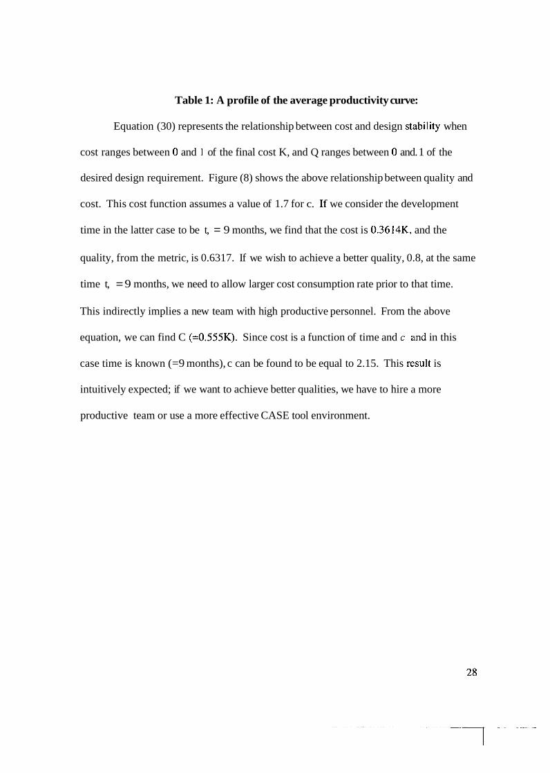
Table 1: A profile of the average productivity curve:

Equation (30) represents the relationship between cost and design stability when

cost ranges between 0 and 1 of the final cost K, and Q ranges between 0 and. 1 of the

desired design requirement. Figure (8) shows the above relationship between quality and

cost. This cost function assumes a value of 1.7 for c. If we consider the development

time in the latter case to be t, = 9 months, we find that the cost is 0.3614K, and the

quality, from the metric, is 0.6317. If we wish to achieve a better quality, 0.8, at the same

time t, = 9 months, we need to allow larger cost consumption rate prior to that time.

This indirectly implies a new team with high productive personnel. From the above

equation, we can find C (=0.555K). Since cost is a function of time and c a~nd in this

case time is known (=9 months), c can be found to be equal to 2.15. This result is

intuitively expected; if we want to achieve better qualities, we have to hire a more

productive team or use a more effective CASE tool environment.

I I I I I I

0 0.1 0.2 0.3 0.4 0.5 0.6 0.7 0.8 Cost

Figure (8) Quality as a Function of Cost

Similar predictions for the other two matrices namely: requirements stability and

fault profile can be made. As a case study, we use the NASA data and find the equations

for R, requirements stability, and F, fault profile in terms the cost, C, as:

R = 1000(2.2065C3 - 3.1434C2 + 1.4738~ + 0.0484) (3 1)

F = 1000(3.11 12C3 - 4.1855C2 + 2 . 0 3 9 ~ + 0.1284) (32) These

equations have been plotted in Figure 9 and 10, and show the same trend as of design

stability metric.

Figure (9) Requirement Stability as a Function of Cost

I I

0.9 - -

0.8 - -

-

>r + .- -

5 +

6 0.5 E 22 .- S O. ~ $

-

-

-

0 I I I I I I I I I

0 0.1 0.2 0.3 0.4 0.5 0.6 0.7 0.8 0.9 1 Cost

-

-

-

-

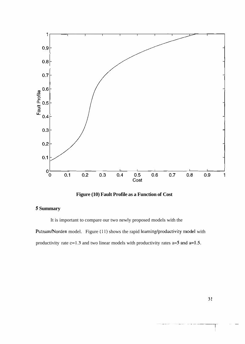
Figure (10) Fault Profile as a Function of Cost

5 Summary

It is important to compare our two newly proposed models with the

Pu tnamorden model. Figure (1 1) shows the rapid leaming/productivity model with

productivity rate c=1.3 and two linear models with productivity rates a=5 and a=1.5.

Figure (11) Rapid LearningIProductivity Curve in Comparison to Two Linear

LearningIProductivity Curves

Figure (12) provides a similar comparison between the average learning/productivity

model with rate c=1.7 and two linear learning/productivity models with same rates as

mentioned above. The corresponding manpower distributions are given in Figures (13)

and (14). It is known that the coding activity phase typically contributes to 42% of the

overall project activities and maintenance activities including rewriting parts of the code

contribute to 48% of the project activities [S].

Time

Figure (12) Average Learning Curve in Comparison to Two linear Learning Curves

Figure (13) Manpower Distribution of Rapid Model in Comparison to Two Linear

model

-0 0.5 1 1.5 2 2.5 3 3.5 4 Time

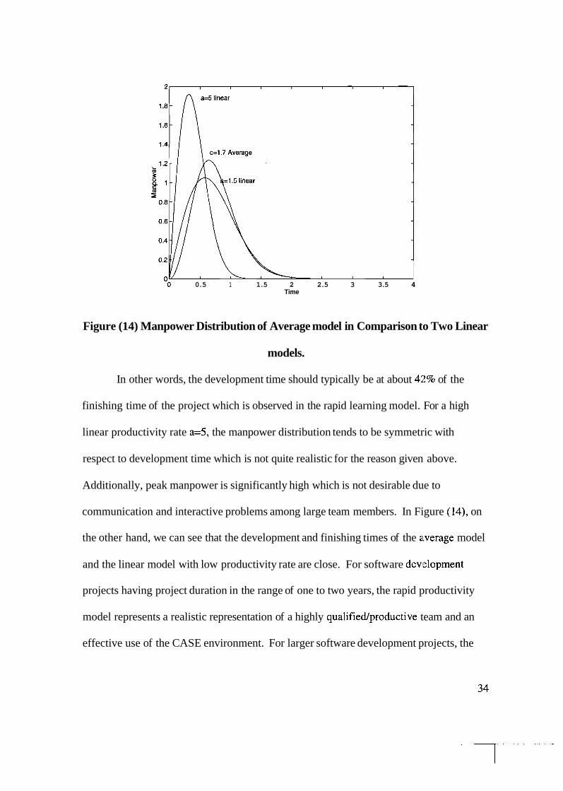
Figure (14) Manpower Distribution of Average model in Comparison to Two Linear

models.

In other words, the development time should typically be at about 42% of the

finishing time of the project which is observed in the rapid learning model. For a high

linear productivity rate a=5, the manpower distribution tends to be symmetric with

respect to development time which is not quite realistic for the reason given above.

Additionally, peak manpower is significantly high which is not desirable due to

communication and interactive problems among large team members. In Figure (14), on

the other hand, we can see that the development and finishing times of the average model

and the linear model with low productivity rate are close. For software devlelopment

projects having project duration in the range of one to two years, the rapid productivity

model represents a realistic representation of a highly qualified/productive team and an

effective use of the CASE environment. For larger software development projects, the

average productivity model is expected to behave better than the linear productivity

model with low learning rates due to the fact that average team personnel improve their

performance later in the project.

5 Conclusion

In summary, our main goal in this report was to represent accuraitely the

human productivity factor in the development of software projects. In previous sections

this factor historically was considered to be either indefinitely growing or was always

constant. Our proposed models introduce a time changing human productivity that grows

for some time and then saturates. It should also be noted that the final cost of a software

development project can be given in terms of program size derived from the: NEC model.

Software development engineers using these proposed models can change quality

requirements as needed. The price is extra cost for paying more experienceld labor. In

this latter case new cost distribution and schedule can be determined a priori. The rapid

productivity model, as discussed above, is a more realistic representation of manpower

distribution than the linear model with high learning rate; whereas the average learning

model is comparable to the linear model with low learning rate in representing the

manpower distribution.

References:

[I] P.V. Norden, "Curve Fitting for a Model of Applied Research and Development

Scheduling," IBM J. Rsch. Dev., Vol. 2, No. 3, July 1958.

[2] P.V. Norden, "Useful Tools for Project Management," in Management of Production,

M.K. Starr, ed. Penguin Books, Baltimore MD, 1970, pp. 71 - 101.

[3] P. V. Norden, "On the Anatomy of Development Projects," IRE Tran. Engr

Management, PGEM, EM-7, March 1960, pp. 34-42.

[4] L. H. Putnam, "A Macro-Estimating Methodology for Software Development,"

Proceedings, IEEE COMPCON 76 Fall, September 1976, pp. 138-143.

[5] L.H. l t n a m "A General Empirical Solution to the Macro Software Sizing and

Estimating Problem," IEEE Tran. Software Engr., July 1978, pp. 345-361.

[6] B. W. Boehm, "Software Engineering Economics," Prentice-Hall, Inc. (1981).

[7] Y. Mizuno, "An Analytical Approach to Software Quality and Productivity

Improvement," IEEE COMPSAC , NEC Corporation, Japan.

[8] B. Londeix, "Cost Estimation for Software Development," Addison-Wesley (1987).

[9] T. K. Abdel-Hamid, "The Dynamics of Software Project Staffing: A S,ystem

Dynamics Based Simulation Approach," IEEE Trans Software Engr., Feb. 1989, pp. 109-

119.

[lo] W. S. Humphrey et al., "Predicting (Individual) Software Productivity," IEEE Tran.

Software Engr., Feb. 1991, pp. 196-207.

[I I] B. Boehm et al., "Characteristics of Software Quality," New York: American

Elsevier, 1978.