effect of liquidity on size premium v7 - forensic economics · 3 the higher the size premium, the...
TRANSCRIPT

Effect of Liquidity on Size Premium and its Implications for Financial Valuations
[** Working Title]
Frank Torchio and Sunita Surana
Preliminary Draft August 2013
2
I. Size Premiums and Fair Value
Discounted Cash Flow (“DCF”) analysis is one of, if not, the key valuation method
taught by academics and used by practitioners. A critical parameter of a DCF analysis is the
weighted average cost of capital (used to discount expected cash flows) which comprises in part
the cost of equity. The cost of equity is generally computed using a version of the capital asset
pricing model (“CAPM”)1, for which the equation is:
Cost of Equity = Risk-free Rate + (Beta x Equity Risk Premium) (1)
Many valuation practitioners generally consider it appropriate to include in the
calculation of the cost of equity a premium based on the market capitalization of equity or size of
the firm being valued. Empirical studies, most notably published in the Ibbotson SBBI
Yearbooks (“Ibbotson SBBI”), have shown that the CAPM alone does not fully account for the
higher historical returns earned by smaller companies.2 These studies show that historical
returns for small firms are systematically greater than the returns implied by their betas (beta-
adjusted returns) from the standard CAPM in (1).
That is, the greater risk of smaller-sized firms is not fully accounted for in the standard
beta calculations for these firms. To account for this size-related effect, one of the variations of
the CAPM equation includes a size premium, defined as:
Cost of Equity = Risk-free Rate + (Beta x Equity Risk Premium) + Size Premium (2)
1 The CAPM is the cornerstone of asset pricing theory and is widely used for the
estimation of cost of capital. See, for example, Sharpe (1964) and Fama and French (2004). 2 See Ibbotson SBBI 2011Valuation Yearbook, pp. 87-90. Banz (1981) first presented
evidence that smaller firms earned higher risk-adjusted returns.

3
The higher the size premium, the higher is the cost of equity, and consequently the lower
is the DCF value, all else the same. Ibbotson SBBI has measured historic size premiums by
constructing portfolios of traded stocks by size. The size premiums are computed as the average
returns for each size portfolio less the average of the returns predicted by CAPM in (1) for the
stocks in each portfolio. Ibbotson has constructed both size-quartile portfolios and size-decile
portfolios. In 2001, Ibbotson refined its size analysis by dividing decile 10, the smallest stock
decile, into 10a and 10b.3 In 2010, Ibbotson further divided the 10th decile into four size
categories: 10w, 10x, 10y, and 10z.4 As can be seen in Table 1, the size premiums increase as
the company size decreases.
3 Ibbotson SBBI 2001Valuation Yearbook, pp. 122-3. 4 Ibbotson SBBI 2010 Valuation Yearbook, p. 91.

4
Table 1 Size Premiums for Size-Quartile and Size-Decile Portfolios
Notes: Source of data is Ibbotson SBBI 2011 Valuation Yearbook. Since the data in our analysis covers the time period 1926-2010, for comparability purposes, throughout this paper we report the statistics from the 2011 Yearbook that uses data also from 1926-2010. Market capitalization in each decile is as of September 30, 2010.
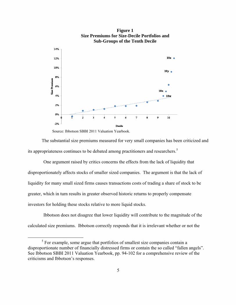
Figure 1 plots the size premiums for the ten deciles (diamonds shapes) and also shows the
size premiums for categories 10w, 10x, 10y, and 10z (circle shapes) contained in the Ibbotson
SBBI 2011 Yearbook. As can be seen in Figure 1, the increase in the size premium is
approximately linear for decile 1 (-0.38%) through decile 9 (2.94%). But for the smallest size
decile (decile 10), the premium increases substantially to 6.36%, which is above the linear trend
line based on the size premiums for deciles 1 through 9. Within decile 10, the increase in size
premiums is even more dramatic and ranges from 3.99% for size category 10w to 12.06% for the
smallest size category, 10z.
Quartile Groups
Size Premium
Decile Groups
Market Capitalization of Largest Company in Decile ($ millions)
Size Premium
1 314,623 -0.38%
2 15,080 0.81%
3 6,794 1.01%
4 3,711 1.20%
5 2,509 1.81%
6 1,776 1.82%
7 1,212 1.88%
8 772 2.65%
9 478 2.94%
10w 236 3.99%
10x 179 4.96%
10y 143 9.15%
10z 86 12.06%
Micro Cap (9-10)
4.07%
Large Cap (1-2)
n/a
Mid Cap (3-5)
1.20%
Low Cap (6-8)
1.98%
5
Figure 1 Size Premiums for Size-Decile Portfolios and
Sub-Groups of the Tenth Decile
Source: Ibbotson SBBI 2011 Valuation Yearbook.
The substantial size premiums measured for very small companies has been criticized and
its appropriateness continues to be debated among practitioners and researchers.5
One argument raised by critics concerns the effects from the lack of liquidity that
disproportionately affects stocks of smaller sized companies. The argument is that the lack of
liquidity for many small sized firms causes transactions costs of trading a share of stock to be
greater, which in turn results in greater observed historic returns to properly compensate
investors for holding these stocks relative to more liquid stocks.
Ibbotson does not disagree that lower liquidity will contribute to the magnitude of the
calculated size premiums. Ibbotson correctly responds that it is irrelevant whether or not the
5 For example, some argue that portfolios of smallest size companies contain a
disproportionate number of financially distressed firms or contain the so called “fallen angels”. See Ibbotson SBBI 2011 Valuation Yearbook, pp. 94-102 for a comprehensive review of the criticisms and Ibbotson’s responses.
6
computed size premium also reflects the lower liquidity in smaller-sized companies when
computing a stock’s fair market value; the return to equity used to compute fair market value
should include the additional return required to compensate investors for holding less liquid
stocks.6 This is because these transactions costs are real, can be substantial, and will affect the
prices paid for a share of stock.7 For example, if an investor were contemplating a purchase of
10 shares of a privately held company, the investor would certainly take into account in the
purchase price she pays the transaction costs she would have to incur in order to sell those shares
at a later time. So, to the extent that the computed size premium includes the effects of less
liquid stocks is largely irrelevant because it is generally appropriate that a fair market valuation
reflect any illiquidity effect on the expected return.
In certain circumstances, however, the purpose of valuation is not to assess the fair
market value, but rather to analyze and compute “fair value”. For example, the appropriate
measure of value in an appraisal for a merger is not fair market value but rather “fair value”. The
key differences between fair market value and fair value are that fair value requires that there be:
(1) no discount -- either direct or implied -- for the lack of liquidity; and (2) no discount for
minority interest.8
6 According to valuation literature, “fair market value” is generally defined as: “…the
amount at which property would change hands between a willing seller and a willing buyer when neither is acting under compulsion and when both have reasonable knowledge of the relevant facts.” See Pratt (2008), pp. 41-42.
7 Under the standard of fair market value, the focus must be on the specific property (ownership interest) being valued, basically “as is,” including control and marketability characteristics. Therefore, minority interests in closely held corporations or partnerships are valued to reflect lack of control and lack of marketability characteristics. See Pratt (2009), p. 10.
8 See Laro and Pratt (2011), pp. 12-13.

7
Therefore, there is general agreement that the fair value of even a completely illiquid,
privately held stock in an appraisal should not reflect any discount to the valuation that would
obtain for the same stock that traded in a completely liquid market. But, if a key valuation
parameter -- the cost of equity -- includes a premium for low liquidity, then the valuation
obtained will necessarily reflect a discount for illiquidity.
Is the value obtained from such an analysis the “fair value” of the stock if that value
reflects an implicit discount for illiquidity? Because fair value is a legal concept, the answer to
this question is left to the courts and legal scholars. This paper, however, provides an economic
context to assist in answering this question by quantifying the liquidity premium reflected in the
size-decile premiums that are currently used by many practitioners. Because the Ibbotson SBBI
Yearbooks are by far the most commonly cited and used source for size premiums, we use the
methods suggested by Ibbotson for computing size premiums and for measuring liquidity.
The rest of the paper is organized as follows. The next section discusses the relationship
between liquidity and asset pricing. The third section describes the data. Liquidity premiums,
without accounting for size, are calculated in the fourth section. The fifth section discusses the
replication of size premiums contained the Ibbotson SBBI 2011 Yearbook. The sixth section
shows the amount of liquidity premium subsumed in the calculation of size premiums for size-
decile portfolios and for the sub-groups of the tenth decile. Finally, the last section provides
concluding remarks.
II. Liquidity and Asset Pricing
The marketability or liquidity of an asset refers to the degree to which it can be converted
to cash quickly without incurring large transaction costs or price concessions. Financial theory
reasons that liquidity affects asset prices because investors price securities according to their
8
returns net of trading costs, such as transactions costs and expected price concessions, and
consequently investors require a greater return for higher expected costs of achieving liquidity,
all else the same. Thus, given two assets with the same expected cash flows but with different
liquidity, investors will pay less (demand a higher return) to hold the more illiquid asset.
Over the last 15 years, liquidity has been the subject of considerable research in the
financial literature. Many of these studies are discussed by Amihud, Mendelson, and Pedersen
(2005) who review the literature concerning the effects of liquidity on asset prices.
Thus, financial economists expect that asset and security prices will differ systematically
depending on the marketability characteristics of the securities, all else equal. For example,
restricted stock should be priced at a discount from the unrestricted stock’s traded “market” price
on a liquid exchange. Indeed, many empirical studies of restricted stock, of the relationship
between stock returns and bid-ask spreads, of a company’s block transactions, and of private
sales of a company’s stock prior to the company’s initial public offering have confirmed that
high transaction costs and other restrictions generally cause securities to be priced at significant
discounts from the market prices of comparable (often otherwise identical) liquid securities.
Table 2 summarizes the illiquidity discounts measured in several restricted stock studies.
These studies report median illiquidity discounts for restricted stock of 9% to 45% and means of
13% to 42% based on hundreds of transactions. Because the restricted stock studies provide a
direct measure of the costs of illiquidity, many experts and courts have chosen to rely on these
studies as an empirical guide in selecting illiquidity discounts to apply to the computed value
from a DCF analysis to arrive at a fair market value measure.

9
Table 2 Studies of Restricted Stock Marketability Discounts
Notes: [1] Discounts Involved in Purchases of Common Stock (1966-1969), Institutional Investor Study Report of the Securities and Exchange Commission, H.R. Doc. No. 64, Part 5, 92nd Congress, 1st Session, 1971, pp. 2444-56, cited in Pratt, Reilly and Schweihs (2000), pp. 396-398, 404. [2] Cited in Pratt, Reilly and Schweihs (2000), pp. 398-399, 404. [3] Cited in Pratt, Reilly and Schweihs (2000), pp. 399, 404. [4] Cited in Pratt, Reilly and Schweihs (2000), pp. 400, 404. [5] Cited in Pratt, Reilly and Schweihs (2000), pp. 400, 404. [6] Unpublished study, cited in Pratt, Reilly and Schweihs (2000), pp. 400, 404. [7] Discount for private placement of unregistered shares. Wruck also reports an average premium of 4.1% and median discount of 1.8% for 36 private placements of registered shares. [8] Discount for private placement of restricted shares. Hertzel and Smith also report an average discount of 15.6% for 88 private placements of non-restricted shares. [9] Oliver, R. & Meyers, R. Discounts Seen in Private Placements of Restricted Stock: The Management Planning, Inc., Long-Term Study (1980-1996). Chapter 5 in Reilly and Schweihs (2000), cited in Pratt, Reilly and Schweihs (2000), pp. 401-404. Median is approximate. [10] The 1980-1997 time period is assumed to match the previous study with additional transactions updated. [11] Unregisterd Shares. Bajaj et al. also report discounts for 37 private placements of registered shares of 14% (average) and 10% (median). [12] Study obtained from Columbia Financial Advisors, Inc. [13] Unpublished study, cited in Laro and Pratt (2005), p.289. [14] Unpublished study, cited in Laro and Pratt (2011), p. 287. [15] Unpublished study, cited in Laro and Pratt (2011), p. 287.
StudyTime
PeriodSample
SizePrice
DiscountGroup
AveragePrice
DiscountGroup
Average
SEC overall average (1971)1
Jan 1966 - June 1969 398 n/a 25.8%Gelman (1972) 1968 - 1970 89 33.0% 33.0%
Trout (1977)2
1968 - 1972 60 n/a 33.5%
Moroney (1973)3
na 146 33.0% 35.6%
Maher (1976)4
1969 - 1973 n/a n/a 35.4%
Pittock and Stryker (1983)5
Oct 1978 - June 1982 28 45.0% n/a
Willamette Management Associates6
Jan 1981 - May 1984 33 31.2% n/a
Wruck (1989)7
July 1979 - Dec 1985 37 12.2% 13.5%
Hertzel and Smith (1983)8
Jan 1980 - May 1987 18 n/a 42.0%Silber (1991) 1981 - 1988 69 n/a 33.8%Hall and Polacek (1994) 1979 - Apr 1992 100+ n/a 23.0%
Oliver and Meyers (2000)9
Jan 1980 - Dec 1996 53 25.0% 27.1%Robak and Hall (2001) 1980 - Apr 1997 230 20.1% 22.3%
Hall (2003)10 1980 - 1997 238 21.3% n/a
Hall and Polacek (1994) May 1991 - Apr 1992 17 n/a 21.0%
Bajaj, Denis, Ferris and Sarin (2001)11 Jan 1990 - Dec 1995 51 26.5% 28.1%
Johnson (1999) 1991 - 1995 72 n/a 20.2%
Finnerty (2003) Jan 1991 - Feb 1997 101 15.5% 20.1%
Aschwald (2000) Jan 1996 - Apr 1997 23 14.0% 21.0%Aschwald (2000) Jan 1997 - Dec 1998 15 9.0% 13.0%
Columbia Financial Advisors, Inc.12 June 1997 - June 2000 32 11.7% 13.5%
Columbia Financial Advisors, Inc.12 Jan 1999 - June 2000 24 11.7% 13.7%
Hall (2003) 1997 - 2000 182 25.9% n/a
FMV Opinions13 1997 - 2003 187 n/a 22.5%
FMV Opinions14 1997 - 2007 311 n/a 20.6%
Post 2007Studies
(six month holding period)
FMV Opinions15 2008 43 n/a n/a 12.6% 12.6%
1990-1997Studies
18.7% 22.1%
1997-2007Studies
(one year holding period)
14.6% 16.7%
Long-Horizon Studies
22.1% 24.1%
Median Average
Pre-1990Studies
30.9% 31.6%

10
The consensus in the liquidity literature is that theory and empirical evidence strongly
support three findings. First, investors require returns that compensate for the level of illiquidity
of an investment.9
Second, stocks in publicly traded equity markets can have substantially different degrees
of liquidity; liquidity is not a binary variable. That is, one cannot simply divide stocks into two
categories of liquidity based solely on whether or not the stock is publicly traded. While stocks
that are not publicly traded are generally characterized as illiquid, even among publicly traded
stocks, there can be important and substantial differences in the degree of liquidity.10
Third, illiquidity is correlated with size. That is, across all publicly traded stocks, more
small stocks tend to have lower liquidity than do large stocks.11 Practitioners and academics are
in general agreement that the negative relationship between returns and liquidity is stronger for
smaller stocks. In a recent study, Ibbotson et al. (2013) empirically studied the effect on returns
from differing levels of liquidity across all size quartile portfolios of publicly traded stocks
between 1972 and 2011. Their findings are presented in Table 3. Ibbotson et al. found that
within each size quartile portfolio, low liquidity portfolios generally earned higher returns than
the high liquidity portfolios. The authors, however, find that the size impact is quite inconsistent
across various levels of liquidity. Specifically, while among low liquidity stocks, small-sized
stock portfolios earned higher returns than the large stock portfolios, the opposite is true for high
9 The effect of liquidity on asset prices was first examined by Amihud and Mendelson
(1986). See also Datar, Naik, and Radcliffe (1998) and Amihud, Mendelson, and Pedersen (2005).
10 For example, Amihud and Mendelson (1986) divide publicly traded stocks into seven liquidity groups that show “significant variability”.
11 See, for example, Amihud (2002) and Ibbotson et al. (2013).

11
liquidity stocks. Thus, based on Ibbotson et al. (2013), at high levels of liquidity, the effect of
small size does not result in higher returns compared to the larger firms.
Table 3 Annualized Arithmetic Return for Size and Liquidity Quartile Portfolios
from Ibbotson et al. (2013)
Source: Ibbotson, R.G., Chen, Z., Kim, D. Y.-J., and Hu, W.Y., 2013. Liquidity as an Investment Style. Financial Analysts Journal, 69(3), Table 2 (partial).
Ibbotson et al. (2013) conclude:
Therefore, size does not capture liquidity (i.e., the liquidity premium holds regardless of size group). Conversely, the size effect does not hold across all liquidity quartiles, especially in the highest-turnover quartile. The liquidity effect, however, is strongest among microcap stocks and declines from micro- to small- to mid- to large-cap stocks.
The key finding implied by Ibbotson et al. (2013) is that for smaller-sized companies the
historic returns are substantially different between low liquidity and high liquidity stocks (first
row of Table 3). If the CAPM returns are not similarly different across the various liquidity
groups, then it implies that a substantial portion of the measure of what is generally referred to as
size premium subsumes the premium that compensates investors for holding low liquidity stocks.
II.a Liquidity Premium Creates an Illiquidity Discount to the Stock’s Valuation
If the size premium subsumes a substantial component that compensates investors for
holding less liquid stocks, then inclusion of such a size premium in the cost of equity will
necessarily result in an illiquidity discount to the stock’s fair value. There is no economic
Quartile Low LiquidityMid-Low Liquidity
Mid-High Liquidity
High Liquidity
Micro Cap 17.92% 20.00% 15.40% 6.78%
Small Cap 17.07% 16.82% 15.38% 9.89%
Mid Cap 15.01% 15.34% 14.51% 11.66%
Large Cap 12.83% 12.86% 12.81% 11.58%
12
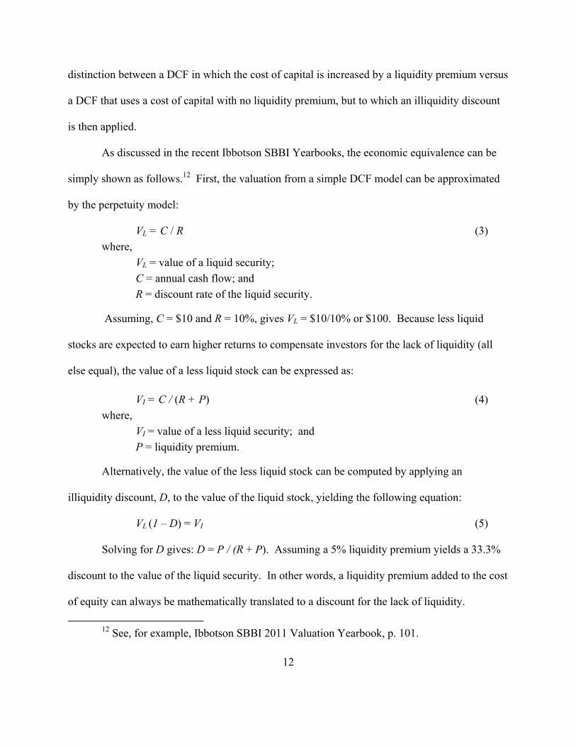
distinction between a DCF in which the cost of capital is increased by a liquidity premium versus
a DCF that uses a cost of capital with no liquidity premium, but to which an illiquidity discount
is then applied.
As discussed in the recent Ibbotson SBBI Yearbooks, the economic equivalence can be
simply shown as follows.12 First, the valuation from a simple DCF model can be approximated
by the perpetuity model:
VL = C / R (3)
where,
VL = value of a liquid security;
C = annual cash flow; and
R = discount rate of the liquid security.
Assuming, C = $10 and R = 10%, gives VL = $10/10% or $100. Because less liquid
stocks are expected to earn higher returns to compensate investors for the lack of liquidity (all
else equal), the value of a less liquid stock can be expressed as:
VI = C / (R + P) (4)
where,
VI = value of a less liquid security; and
P = liquidity premium.
Alternatively, the value of the less liquid stock can be computed by applying an
illiquidity discount, D, to the value of the liquid stock, yielding the following equation:
VL (1 – D) = VI (5)
Solving for D gives: D = P / (R + P). Assuming a 5% liquidity premium yields a 33.3%
discount to the value of the liquid security. In other words, a liquidity premium added to the cost
of equity can always be mathematically translated to a discount for the lack of liquidity.
12 See, for example, Ibbotson SBBI 2011 Valuation Yearbook, p. 101.
13
There are two inferences from this simple economic equivalence. First, if one is
computing the fair value of a privately held stock, it is duplicative to apply a full illiquidity
discount factor to a DCF valuation when the DCF uses a cost of equity that includes a liquidity
premium. Second, if one is computing the fair value of a stock, the fair value computation will
reflect an implicit discount for lack of liquidity if the cost of equity includes a liquidity premium.
In the following sections we empirically investigate the magnitude of the liquidity
premium.
III. Data Description
We use monthly common stock data from 1926 through 2010 compiled by the Center for
Research in Security Prices (“CRSP”) at the University of Chicago Booth School of Business.
All common stock traded on the New York Stock Exchange (“NYSE”), American Stock
Exchange (“AMEX”)13, and NASDAQ stock markets are used. From 1926 through 2010, over 3
million monthly-level observations are available.
Monthly returns on the Standard & Poor’s (“S&P”) 500 index and 30-day U.S. Treasury
bill total return from 1926 through 2010 are also obtained from CRSP. Finally, long-term mean
income return component of 20-year government bonds and long-term equity risk premia are
obtained from Ibbotson SBBI 2011 Valuation Yearbook.
For the analysis of adjustment to NASDAQ volume to account for the potential over-
counting of traded volume, we use daily common stock data from 1990 through 2012 from
CRSP. For this time period, over 40 million daily-level observations are available.
13 In October 2008, AMEX was acquired by NYSE Euronext.

14
III.a Adjustment to NASDAQ Volume
Volumes in quote-driven dealer markets like NASDAQ were historically higher than
order-driven markets like NYSE because public buyers and sellers traded though the
intermediation of dealers on NASDAQ, leading to an over count of trades among public traders.
On NYSE, public buyers and sellers mostly traded among themselves. The differing market
structures caused higher volumes for NASDAQ stocks, all else equal. However, regulatory
interventions by the SEC (e.g., the 1997 SEC mandated order handling rules at NASDAQ14) as
well as the rapid growth of electronic trading mechanisms have caused the trading patterns on
different platforms to converge.
Ibbotson et al. (2013) divide volumes of NASDAQ stocks based on an adjustment factor
suggested by Anderson and Dyl (2005). Based on stocks switching from NASDAQ to NYSE
from 1997 through 2002, Anderson and Dyl find that the mean daily volume declined an average
of 24.7% and the median decrease was 37.9%. Further, based on the finding in Anderson and
Dyl (2007) that the relative over-reporting of NASDAQ stocks has not lessened during 2003-
2005 relative to the 1990-1996 time period, Ibbotson et al. (2013) apply the adjustment factor
throughout their study period of 1972-2011. While Anderson and Dyl (2007) found no evidence
that the over-reporting has lessened for NASDAQ stocks, using data from 1993-2010, Harris
(2011) reports that over time volumes between NYSE and NASDAQ stocks have become more
and more similar leading to the homogenization of US equity markets.
In light of the differences in the findings in Harris (2011) and Anderson and Dyl (2007)
and the vast changes in the stock trading landscape, we analyzed the volume of common stocks
14 See, for example, McInish, Van Ness, and Van Ness (1998).

15
switching from NASDAQ to NYSE starting in 1990 (since the regulatory changes likely to
impact the over counting of traded volume and the rapid growth of electronic trading
mechanisms occurred after 1990). We studied volume on sixty trading days before and after the
switch (with day one being the day of the switch). For each company switching from NASDAQ
to NYSE, average volume during 60 trading days before the switch is divided by average volume
during 60 trading days after the switch. The ratio of the two volumes is shown in figure 2. The
horizontal lines represent the median ratios for consecutive five year periods beginning in 1990.
As is evident from the figure and consistent with Harris (2011), the ratio has been decreasing
over time.

16
Figure 2 Average Volume on NASDAQ Before the Switch Divided by
Average Volume on NYSE After the Switch
Note: In order to focus on presenting the medians, the figure shows ratios between 0 and 4. A few outliers (greater than 4) are not shown in the figure but are used in the computation of the median ratios.
We use the median ratios over five year intervals to adjust NASDAQ volume.
Specifically, the ratio of 2.07 is used to divide NASDAQ volume prior to 1994; 1.75 is used to
divide NASDAQ volume between 1995 and 1999; 1.38 is used to divide NASDAQ volume
between 2000 and 2004; 1.32 is used to divide NASDAQ volume between 2005 and 2009; and
1.21 is used to divide NASDAQ volume after 2009.
0
1
2
3
4
1985 1990 1995 2000 2005 2010 2015
2.07
1.75
1.38 1.32
1.21
Median
17
IV. Liquidity Premium
We measure liquidity using average monthly share turnover in each quarter.15 Share
turnover is calculated as the volume of shares traded each month divided by the number of shares
outstanding at each month-end. This measure of liquidity is similar to the one used in Ibbotson
et al. (2013), except that whereas Ibbotson et al. (2013) create annual portfolios of stocks and
hence measure liquidity annually, we create portfolios of stocks that are rebalanced quarterly in
keeping with the size premium methodology in the Ibbotson SBBI Yearbooks, and hence, we
update the liquidity measure each quarter. The steps we take to create the liquidity-based
portfolios of stocks are described below.
We first rank companies with primary listings on the NYSE based on their liquidity at the
end of each quarter. As mentioned above, liquidity at the end of each quarter is measured as
average monthly share turnover in that quarter.
Second, based on these rankings, the companies are divided into two equally populated
groups based on the median liquidity at the end of each quarter. Group “H” contains companies
with liquidity greater than or equal to the median liquidity, or the high liquidity companies.
Group “L” contains companies with liquidity lower than the median liquidity, or the low
liquidity companies. The ranking of the stocks thus yields a liquidity cutoff demarcating the
“H” and “L” groups at the end of each quarter. These liquidity cutoffs obtained from NYSE
stocks are then used to assign common stocks listed on AMEX and Nasdaq to one of the two
liquidity groups based on the end of quarter liquidity measure for the AMEX and Nasdaq stocks.
15 Turnover rates and bid-ask spreads are typically used as measures of liquidity. See
Amihud et al. (2005). Another measure of liquidity is the price impact such as the ratio of absolute stock return to its dollar volume, averaged over some period (Amihud, 2002).
18
Third, the liquidity groupings are rebalanced quarterly. Each month, every company is
assigned a liquidity group based on its liquidity categorization in the previous quarter. For
example, the liquidity category that a company falls under as of the quarter ending in March is
used to assign its liquidity group for April, May, and June of that year. Thus, each stock remains
in the same liquidity group for each of the three months that follow its assignment to a liquidity
group using the liquidity measure from the end of the previous quarter. This methodology is
similar to the methodology used by CRSP and the Ibbotson SBBI Yearbooks for the creation of
the size-decile portfolios (discussed further below).
Fourth, we compute monthly portfolio returns as the average returns of the stocks in each
liquidity group from 1926 to 2010. Annual portfolio returns are computed by compounding the
monthly returns.16
Fifth, to compute the risk-adjusted portfolio returns, we compute the beta for each
liquidity portfolio using the single-factor CAPM model. Following the SBBI Yearbooks, we use
the following single-factor regression equation to estimate each portfolio’s systematic risk
(commonly referred to in the literature as the portfolio’s beta).
(rl – rf) = αl + βl (rm – rf) + εl (5)
where, rl represents monthly return on portfolio l; rf represents 30-day U.S. treasury bill total return; and rm represents monthly return on the market, measured by the S&P 500 index.
The slope of the regression, βl, in equation (5) measures the portfolio’s sensitivity to
variations in the market return, or its exposure to systematic risk.
16 Annual return is computed when monthly return data is available for each of the twelve
months.

19
Using the beta for each liquidity portfolio, βl, a CAPM portfolio return (in excess of the
riskless rate) is computed as the product of the estimated beta for that portfolio and the equity
risk premium (the difference between the mean total return of the S&P 500 index and the mean
income return component of 20-year government bonds for the time period 1926-2010).
Finally, for each liquidity portfolio of stocks, we calculate the difference between the
portfolio’s actual average annual return in excess of the risk-free rate (measured by the mean
income return component of 20-year government bonds for the time period 1926-2010) and the
CAPM return also in excess of the risk-free rate. We refer to this difference as the liquidity
premium. Table 4 presents the liquidity premiums for the “H” and “L” liquidity groups. We
find that while the high liquidity stocks have a liquidity premium of less than 1%, the liquidity
premium for the low liquidity stocks is over 7%.
Table 4 Long-Term Returns in Excess of Estimated CAPM Returns for
High and Low Liquidity Categories
Notes: Historical riskless rate is measured by the arithmetic mean income return component of the 20-year government bond (5.17%). Long horizon equity risk premium is estimated by the arithmetic mean total return of the S&P 500 (11.88%) minus the arithmetic mean income return component of the 20-year government bond (5.17%).
Using the same methodology described above, we also categorize the data into liquidity
quartiles. The results are presented in Table 5. Again, we find that liquidity premium increases
Liquidity Group Beta
Actual Arithmetic
Mean Return
Actual Return in Excess of
Riskless Rate
CAPM Return in Excess of
Riskless Rate
Liquidity Premium (Return in Excess of CAPM Return)
[1] [2] [3] [4] = [3] - 5.17%[5] = β *
(11.88% - 5.17%)[6] = [4] - [5]
H 1.36 14.95% 9.78% 9.09% 0.69%
L 1.05 19.50% 14.33% 7.02% 7.31%
20
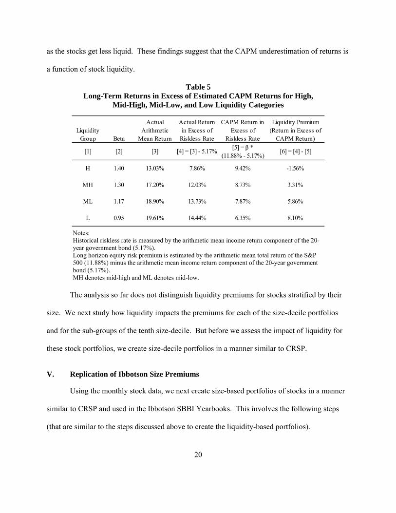
as the stocks get less liquid. These findings suggest that the CAPM underestimation of returns is
a function of stock liquidity.
Table 5 Long-Term Returns in Excess of Estimated CAPM Returns for High,
Mid-High, Mid-Low, and Low Liquidity Categories
Notes: Historical riskless rate is measured by the arithmetic mean income return component of the 20-year government bond (5.17%). Long horizon equity risk premium is estimated by the arithmetic mean total return of the S&P 500 (11.88%) minus the arithmetic mean income return component of the 20-year government bond (5.17%). MH denotes mid-high and ML denotes mid-low.
The analysis so far does not distinguish liquidity premiums for stocks stratified by their
size. We next study how liquidity impacts the premiums for each of the size-decile portfolios
and for the sub-groups of the tenth size-decile. But before we assess the impact of liquidity for
these stock portfolios, we create size-decile portfolios in a manner similar to CRSP.
V. Replication of Ibbotson Size Premiums
Using the monthly stock data, we next create size-based portfolios of stocks in a manner
similar to CRSP and used in the Ibbotson SBBI Yearbooks. This involves the following steps
(that are similar to the steps discussed above to create the liquidity-based portfolios).
Liquidity Group Beta
Actual Arithmetic
Mean Return
Actual Return in Excess of
Riskless Rate
CAPM Return in Excess of
Riskless Rate
Liquidity Premium (Return in Excess of
CAPM Return)
[1] [2] [3] [4] = [3] - 5.17%[5] = β *
(11.88% - 5.17%)[6] = [4] - [5]
H 1.40 13.03% 7.86% 9.42% -1.56%
MH 1.30 17.20% 12.03% 8.73% 3.31%
ML 1.17 18.90% 13.73% 7.87% 5.86%
L 0.95 19.61% 14.44% 6.35% 8.10%

21
Using monthly data from 1926-2010, we first rank the companies with primary listings
on the NYSE based on their market capitalizations at the end of each quarter. Market
capitalization is calculated as the product of the closing price on the last trading date of the
quarter and the shares outstanding.17
Second, based on these rankings, the companies are divided into equally populated
deciles (decile 1 contains the largest companies, and decile 10 the smallest). Thus, the ranking
of the NYSE stocks yield size cutoffs for each decile, where the cutoffs are the highest and
lowest market capitalizations within each size-decile. These decile cutoffs obtained from NYSE
stocks are then used to assign common stocks listed on AMEX and Nasdaq to one of the size
deciles based on the end of fiscal quarter market capitalization for the AMEX and Nasdaq stocks.
Third, size-decile portfolios are constructed for the stocks based on the size-decile
rankings. Each month, every company is assigned a portfolio based on its decile ranking in the
previous quarter. For example, the decile ranking of a stock based on its market capitalization as
of the quarter ending in March is used to determine the stock’s size-decile for the months of
April, May, and June. Thus, each stock remains in the same size-decile for each of three months
that follow its assignment to a size-decile using the market capitalization from the end of the
previous quarter.
Fourth, monthly portfolio returns are computed as the weighted average returns of the
stocks in each size-decile, using market capitalizations based on the shares outstanding and
17 In the calculation of the liquidity portfolios discussed above we calculated the average
monthly share turnover over a quarter instead of just using the last month in the quarter in order to preserve observations in the analysis that otherwise would be lost due to missing volume data in the last months of the quarters.
22
closing price for the last trading day of the previous month as weights. Annual portfolio returns
are computed by compounding the monthly returns.
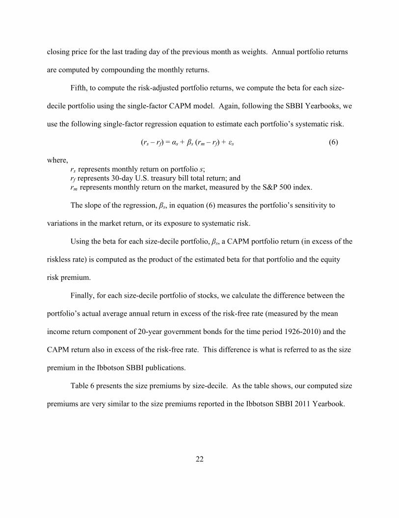
Fifth, to compute the risk-adjusted portfolio returns, we compute the beta for each size-
decile portfolio using the single-factor CAPM model. Again, following the SBBI Yearbooks, we
use the following single-factor regression equation to estimate each portfolio’s systematic risk.
(rs – rf) = αs + βs (rm – rf) + εs (6)
where, rs represents monthly return on portfolio s; rf represents 30-day U.S. treasury bill total return; and rm represents monthly return on the market, measured by the S&P 500 index.
The slope of the regression, βs, in equation (6) measures the portfolio’s sensitivity to
variations in the market return, or its exposure to systematic risk.
Using the beta for each size-decile portfolio, βs, a CAPM portfolio return (in excess of the
riskless rate) is computed as the product of the estimated beta for that portfolio and the equity
risk premium.
Finally, for each size-decile portfolio of stocks, we calculate the difference between the
portfolio’s actual average annual return in excess of the risk-free rate (measured by the mean
income return component of 20-year government bonds for the time period 1926-2010) and the
CAPM return also in excess of the risk-free rate. This difference is what is referred to as the size
premium in the Ibbotson SBBI publications.
Table 6 presents the size premiums by size-decile. As the table shows, our computed size
premiums are very similar to the size premiums reported in the Ibbotson SBBI 2011 Yearbook.

23
Table 6 Comparison of Ibbotson SBBI and Torchio-Surana Long-Term Returns in Excess of
Estimated CAPM Returns for Size-Decile Portfolios
Notes: Historical riskless rate is measured by the arithmetic mean income return component of the 20-year government bond (5.17%). Long horizon equity risk premium is estimated by the arithmetic mean total return of the S&P 500 (11.88%) minus the arithmetic mean income return component of the 20-year government bond (5.17%).
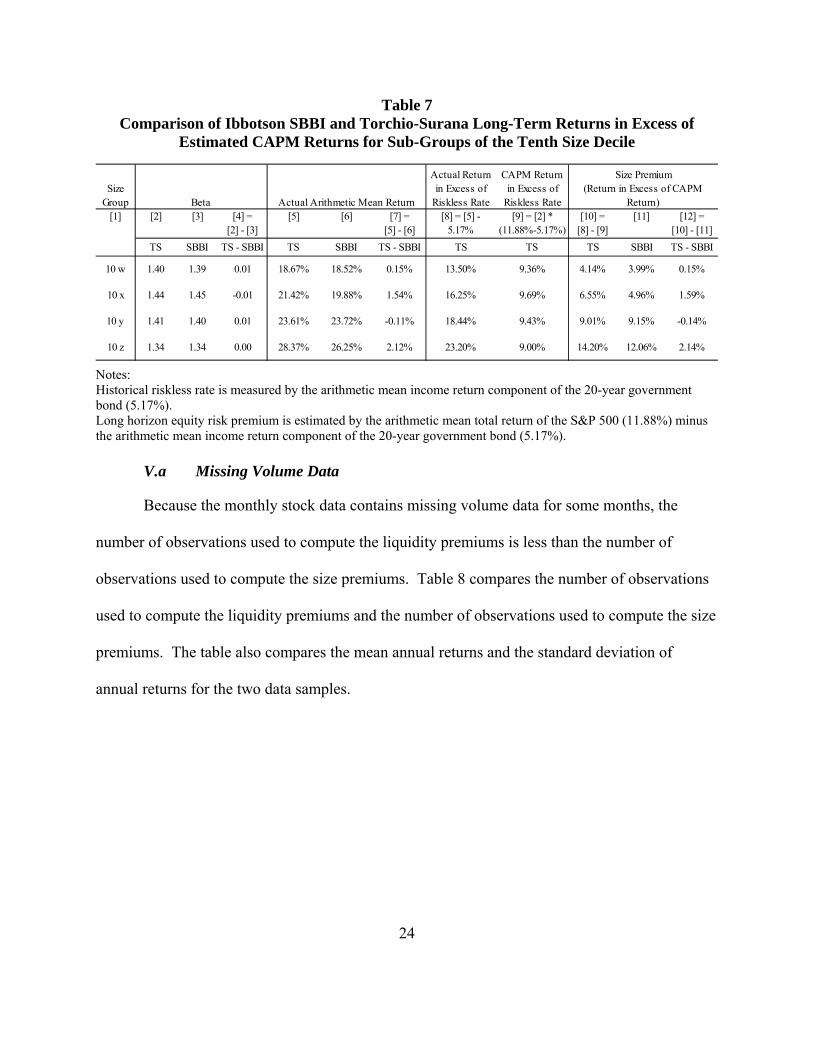
As discussed above, Ibbotson divides the smallest size-decile, decile 10, into 4 size sub-
groups (10w, 10x, 10y, and 10z) using the same methodology that is used to construct the 10
size-decile portfolios. In Table 7, we replicate that analysis and show the computed size
premiums for sub-size groups w, x, y, and z for decile 10 are quite close to the size premiums
reported in the Ibbotson SBBI 2011 Yearbook. One reason for the differences between our
estimates and those reported in the Ibbotson SBBI Yearbook is that Ibbotson SBBI uses its
internal database of companies for the sub-groups of the tenth decile (based on email
communication with Morningstar). Notwithstanding the differences, the results are wholly
consistent with that from Ibbotson.
Decile
Actual Return in Excess of
Riskless Rate
CAPM Return in Excess of
Riskless Rate[1] [2] [3] [4] =
[2] - [3][5] [6] [7] =
[5] - [6][8] = [5] - 5.17% [9] = [2] *
(11.88%-5.17%)[10] =
[8] - [9][11] [12] =
[10] - [11]TS SBBI TS - SBBI TS SBBI TS - SBBI TS TS TS SBBI TS - SBBI
1 0.92 0.91 0.01 10.87% 10.92% -0.05% 5.70% 6.15% -0.44% -0.38% -0.06%
2 1.03 1.03 0.00 13.02% 12.92% 0.10% 7.85% 6.89% 0.96% 0.81% 0.15%
3 1.10 1.10 0.00 13.44% 13.56% -0.12% 8.27% 7.40% 0.88% 1.01% -0.13%
4 1.13 1.12 0.01 14.04% 13.91% 0.13% 8.87% 7.57% 1.30% 1.20% 0.10%
5 1.17 1.16 0.01 14.66% 14.75% -0.09% 9.49% 7.82% 1.67% 1.81% -0.14%
6 1.19 1.19 0.00 14.93% 14.95% -0.02% 9.76% 7.97% 1.79% 1.82% -0.03%
7 1.23 1.24 -0.01 15.24% 15.38% -0.14% 10.07% 8.25% 1.82% 1.88% -0.06%
8 1.30 1.30 0.00 16.20% 16.54% -0.34% 11.03% 8.70% 2.33% 2.65% -0.32%
9 1.34 1.35 -0.01 17.01% 17.16% -0.15% 11.84% 8.99% 2.85% 2.94% -0.09%
10 1.40 1.41 -0.01 21.49% 20.97% 0.52% 16.32% 9.40% 6.93% 6.36% 0.57%
Size Premium (Return in Excess of CAPM Return)Beta Actual Arithmetic Mean Return
24
Table 7 Comparison of Ibbotson SBBI and Torchio-Surana Long-Term Returns in Excess of
Estimated CAPM Returns for Sub-Groups of the Tenth Size Decile
Notes: Historical riskless rate is measured by the arithmetic mean income return component of the 20-year government bond (5.17%). Long horizon equity risk premium is estimated by the arithmetic mean total return of the S&P 500 (11.88%) minus the arithmetic mean income return component of the 20-year government bond (5.17%).
V.a Missing Volume Data
Because the monthly stock data contains missing volume data for some months, the
number of observations used to compute the liquidity premiums is less than the number of
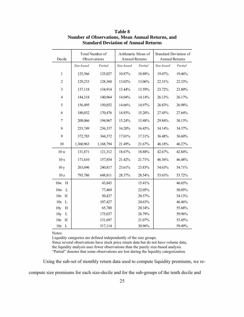
observations used to compute the size premiums. Table 8 compares the number of observations
used to compute the liquidity premiums and the number of observations used to compute the size
premiums. The table also compares the mean annual returns and the standard deviation of
annual returns for the two data samples.
Size Group
Actual Return in Excess of
Riskless Rate
CAPM Return in Excess of
Riskless Rate[1] [2] [3] [4] =
[2] - [3][5] [6] [7] =
[5] - [6][8] = [5] -
5.17%[9] = [2] *
(11.88%-5.17%)[10] =
[8] - [9][11] [12] =
[10] - [11]
TS SBBI TS - SBBI TS SBBI TS - SBBI TS TS TS SBBI TS - SBBI
10 w 1.40 1.39 0.01 18.67% 18.52% 0.15% 13.50% 9.36% 4.14% 3.99% 0.15%
10 x 1.44 1.45 -0.01 21.42% 19.88% 1.54% 16.25% 9.69% 6.55% 4.96% 1.59%
10 y 1.41 1.40 0.01 23.61% 23.72% -0.11% 18.44% 9.43% 9.01% 9.15% -0.14%
10 z 1.34 1.34 0.00 28.37% 26.25% 2.12% 23.20% 9.00% 14.20% 12.06% 2.14%
Size Premium (Return in Excess of CAPM
Return)Beta Actual Arithmetic Mean Return
25
Table 8 Number of Observations, Mean Annual Returns, and
Standard Deviation of Annual Returns
Notes: Liquidity categories are defined independently of the size groups. Since several observations have stock price return data but do not have volume data, the liquidity analysis uses fewer observations than the purely size-based analysis. “Partial” denotes that some observations are lost during the liquidity categorization.
Using the sub-set of monthly return data used to compute liquidity premiums, we re-
compute size premiums for each size-decile and for the sub-groups of the tenth decile and
DecileTotal Number of
ObservationsArithmetic Mean of
Annual ReturnsStandard Deviation of
Annual Returns
Size-based Partial Size-based Partial Size-based Partial
1 125,566 125,027 10.87% 10.88% 19.47% 19.46%
2 129,233 128,360 13.02% 13.06% 22.31% 22.33%
3 137,118 134,914 13.44% 13.59% 23.72% 23.80%
4 144,318 140,964 14.04% 14.14% 26.13% 26.17%
5 156,495 150,852 14.66% 14.97% 26.83% 26.98%
6 180,032 170,476 14.93% 15.20% 27.45% 27.64%
7 208,066 194,967 15.24% 15.48% 29.84% 30.13%
8 253,749 236,337 16.20% 16.45% 34.14% 34.37%
9 372,783 344,372 17.01% 17.31% 36.48% 36.60%
10 1,360,963 1,168,794 21.49% 21.67% 46.18% 46.27%
10 w 131,871 121,312 18.67% 18.88% 42.67% 42.84%
10 x 171,610 157,854 21.42% 21.71% 46.36% 46.48%
10 y 263,696 240,817 23.61% 23.83% 54.63% 54.71%
10 z 793,786 648,811 28.37% 28.54% 53.63% 53.72%
10w H 43,843 15.41% 46.65%
10w L 77,469 22.05% 50.05%
10x H 50,427 20.57% 54.13%
10x L 107,427 24.63% 46.46%
10y H 65,780 20.34% 55.68%
10y L 175,037 26.79% 59.96%
10z H 131,697 21.07% 53.45%
10z L 517,114 30.96% 59.49%
26
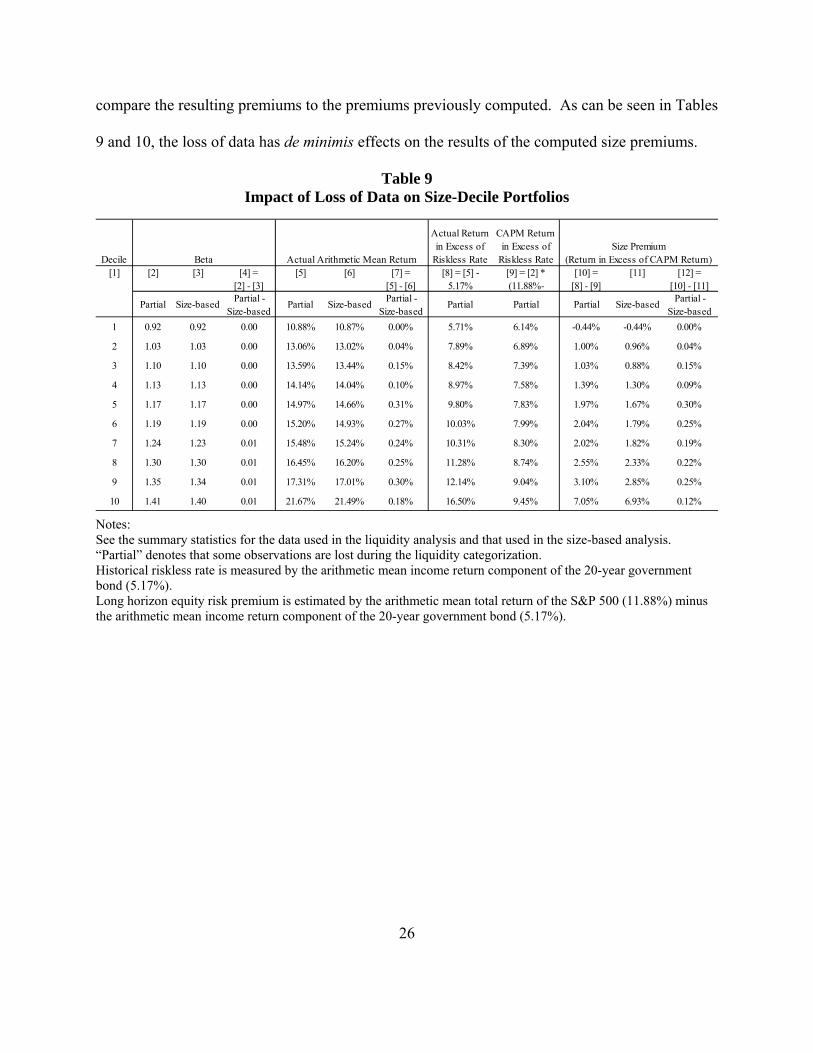
compare the resulting premiums to the premiums previously computed. As can be seen in Tables
9 and 10, the loss of data has de minimis effects on the results of the computed size premiums.
Table 9 Impact of Loss of Data on Size-Decile Portfolios
Notes: See the summary statistics for the data used in the liquidity analysis and that used in the size-based analysis. “Partial” denotes that some observations are lost during the liquidity categorization. Historical riskless rate is measured by the arithmetic mean income return component of the 20-year government bond (5.17%). Long horizon equity risk premium is estimated by the arithmetic mean total return of the S&P 500 (11.88%) minus the arithmetic mean income return component of the 20-year government bond (5.17%).
Decile
Actual Return in Excess of
Riskless Rate
CAPM Return in Excess of
Riskless Rate[1] [2] [3] [4] =
[2] - [3][5] [6] [7] =
[5] - [6][8] = [5] -
5.17%[9] = [2] * (11.88%-
[10] = [8] - [9]
[11] [12] = [10] - [11]
Partial Size-basedPartial -
Size-basedPartial Size-based
Partial - Size-based
Partial Partial Partial Size-basedPartial -
Size-based
1 0.92 0.92 0.00 10.88% 10.87% 0.00% 5.71% 6.14% -0.44% -0.44% 0.00%
2 1.03 1.03 0.00 13.06% 13.02% 0.04% 7.89% 6.89% 1.00% 0.96% 0.04%
3 1.10 1.10 0.00 13.59% 13.44% 0.15% 8.42% 7.39% 1.03% 0.88% 0.15%
4 1.13 1.13 0.00 14.14% 14.04% 0.10% 8.97% 7.58% 1.39% 1.30% 0.09%
5 1.17 1.17 0.00 14.97% 14.66% 0.31% 9.80% 7.83% 1.97% 1.67% 0.30%
6 1.19 1.19 0.00 15.20% 14.93% 0.27% 10.03% 7.99% 2.04% 1.79% 0.25%
7 1.24 1.23 0.01 15.48% 15.24% 0.24% 10.31% 8.30% 2.02% 1.82% 0.19%
8 1.30 1.30 0.01 16.45% 16.20% 0.25% 11.28% 8.74% 2.55% 2.33% 0.22%
9 1.35 1.34 0.01 17.31% 17.01% 0.30% 12.14% 9.04% 3.10% 2.85% 0.25%
10 1.41 1.40 0.01 21.67% 21.49% 0.18% 16.50% 9.45% 7.05% 6.93% 0.12%
Size Premium (Return in Excess of CAPM Return)Beta Actual Arithmetic Mean Return
27
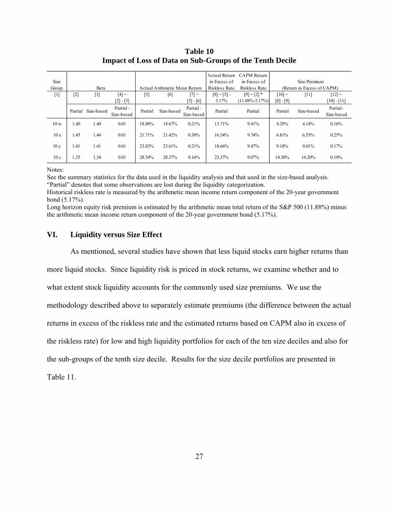
Table 10 Impact of Loss of Data on Sub-Groups of the Tenth Decile
Notes: See the summary statistics for the data used in the liquidity analysis and that used in the size-based analysis. “Partial” denotes that some observations are lost during the liquidity categorization. Historical riskless rate is measured by the arithmetic mean income return component of the 20-year government bond (5.17%). Long horizon equity risk premium is estimated by the arithmetic mean total return of the S&P 500 (11.88%) minus the arithmetic mean income return component of the 20-year government bond (5.17%).
VI. Liquidity versus Size Effect
As mentioned, several studies have shown that less liquid stocks earn higher returns than
more liquid stocks. Since liquidity risk is priced in stock returns, we examine whether and to
what extent stock liquidity accounts for the commonly used size premiums. We use the
methodology described above to separately estimate premiums (the difference between the actual
returns in excess of the riskless rate and the estimated returns based on CAPM also in excess of
the riskless rate) for low and high liquidity portfolios for each of the ten size deciles and also for
the sub-groups of the tenth size decile. Results for the size decile portfolios are presented in
Table 11.
Size Group
Actual Return in Excess of
Riskless Rate
CAPM Return in Excess of
Riskless Rate[1] [2] [3] [4] =
[2] - [3][5] [6] [7] =
[5] - [6][8] = [5] -
5.17%[9] = [2] *
(11.88%-5.17%)[10] =
[8] - [9][11] [12] =
[10] - [11]
Partial Size-basedPartial -
Size-basedPartial Size-based
Partial - Size-based
Partial Partial Partial Size-basedPartial -
Size-based
10 w 1.40 1.40 0.01 18.88% 18.67% 0.21% 13.71% 9.41% 4.29% 4.14% 0.16%
10 x 1.45 1.44 0.01 21.71% 21.42% 0.30% 16.54% 9.74% 6.81% 6.55% 0.25%
10 y 1.41 1.41 0.01 23.83% 23.61% 0.21% 18.66% 9.47% 9.18% 9.01% 0.17%
10 z 1.35 1.34 0.01 28.54% 28.37% 0.16% 23.37% 9.07% 14.30% 14.20% 0.10%
Size Premium (Return in Excess of CAPM)Beta Actual Arithmetic Mean Return
28
Beta
Actual Arithmetic
Mean Return
Actual Return in Excess of
Riskless Rate
CAPM Return in Excess of
Riskless Rate
Premium (Return in Excess of CAPM Return)
[2] [3] [4] = [3] - 5.17%[5] = β *
(11.88% - 5.17%)[6] = [4] - [5]
1 H 1.12 11.32% 6.15% 7.50% -1.35%
L 0.81 10.71% 5.54% 5.41% 0.13%
2 H 1.18 12.92% 7.75% 7.90% -0.16%
L 0.87 13.28% 8.11% 5.87% 2.25%
3 H 1.25 13.49% 8.32% 8.37% -0.05%
L 0.93 14.28% 9.11% 6.22% 2.88%
4 H 1.31 14.04% 8.87% 8.80% 0.07%
L 0.90 14.49% 9.32% 6.07% 3.25%
5 H 1.33 14.66% 9.49% 8.92% 0.57%
L 0.97 15.68% 10.51% 6.50% 4.01%
6 H 1.37 14.04% 8.87% 9.21% -0.33%
L 0.98 16.62% 11.45% 6.55% 4.90%
7 H 1.41 14.68% 9.51% 9.45% 0.06%
L 1.06 16.61% 11.44% 7.10% 4.34%
8 H 1.46 15.19% 10.02% 9.83% 0.19%
L 1.13 18.18% 13.01% 7.61% 5.40%
9 H 1.51 17.27% 12.10% 10.10% 1.99%
L 1.20 18.49% 13.32% 8.08% 5.25%
10 H 1.62 18.52% 13.35% 10.90% 2.46%
L 1.31 25.11% 19.94% 8.76% 11.18%
Group
[1]
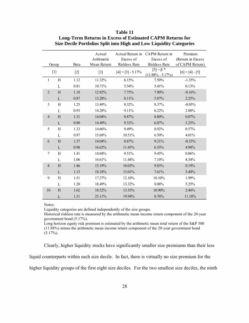
Table 11 Long-Term Returns in Excess of Estimated CAPM Returns for
Size Decile Portfolios Split into High and Low Liquidity Categories
Notes: Liquidity categories are defined independently of the size groups. Historical riskless rate is measured by the arithmetic mean income return component of the 20-year government bond (5.17%). Long horizon equity risk premium is estimated by the arithmetic mean total return of the S&P 500 (11.88%) minus the arithmetic mean income return component of the 20-year government bond (5.17%).
Clearly, higher liquidity stocks have significantly smaller size premiums than their less
liquid counterparts within each size decile. In fact, there is virtually no size premium for the
higher liquidity groups of the first eight size deciles. For the two smallest size deciles, the ninth

29
Beta
Actual Arithmetic
Mean Return
Actual Return in Excess of
Riskless Rate
CAPM Return in Excess of
Riskless Rate
Premium (Return in Excess of CAPM Return)
[2] [3] [4] = [3] - 5.17%[5] = β *
(11.88% - 5.17%)[6] = [4] - [5]
10 w H 1.58 15.41% 10.24% 10.61% -0.37%
L 1.31 22.05% 16.88% 8.80% 8.08%
10 x H 1.61 20.57% 15.40% 10.84% 4.57%
L 1.35 24.63% 19.46% 9.06% 10.40%
10 y H 1.76 20.34% 15.17% 11.83% 3.34%
L 1.31 26.79% 21.62% 8.77% 12.85%
10 z H 1.84 21.07% 15.90% 12.33% 3.57%
L 1.23 30.96% 25.79% 8.24% 17.55%
Group
[1]
and the tenth deciles, the premiums for the high liquidity group are only 2% and 2.5%,
respectively.
Results for each of the sub-groups of the tenth decile (groups 10w, 10x, 10y, and 10z) are
shown in Table 12. As before, for each of the sub-groups of the tenth decile, premiums for the
portfolios of high liquidity stocks are considerably smaller than the premiums for their lower
liquidity counterparts. Indeed, the premium is not greater than 5% in any of the sub-groups’ high
liquidity portfolios of stocks.
Table 12 Long-Term Returns in Excess of Estimated CAPM Returns for
Sub-Groups of the Tenth Size Decile Split into High and Low Liquidity Categories
Notes: Liquidity categories are defined independently of the size groups. Historical riskless rate is measured by the arithmetic mean income return component of the 20-year government bond (5.17%). Long horizon equity risk premium is estimated by the arithmetic mean total return of the S&P 500 (11.88%) minus the arithmetic mean income return component of the 20-year government bond (5.17%). One observation from Tables 11 and 12 is that within each size group the estimated beta
is greater for the high liquidity stocks than for the low liquidity stocks. Since higher liquidity

30
stocks by definition trade more frequently than less liquid stocks, their prices more quickly
reflect the movements of the broader market. Thus, the high liquidity stocks are less prone to the
under-estimation of beta that low liquidity stocks suffer because of a lagged response to the
market movements. Hence, the betas and therefore the estimated CAPM returns are higher for
more liquid stocks than less liquid stocks within the same size portfolio of stocks. Beta estimates
for low liquidity stocks can be improved by accounting for their lagged response to market
movements. We discuss one such methodology in the Appendix.
The second observation from Tables 11 and 12 is that within each size group, the average
actual returns for high liquidity stocks are greater than that for low liquidity stocks. This is
consistent with the findings in the general liquidity literature that investors require compensation
for holding low liquidity stocks, even within the same size group. The higher actual returns
combined with the lower CAPM returns explain the significantly higher premiums for the less
liquid stock relative to their more liquid counterparts within the same size group.
VI.a Comparison of Size Premiums of Higher Liquidity Stocks to Ibbotson SBBI Size Premiums
We next compare the size premiums of higher liquidity stocks to the frequently used size
premiums published in Ibbotson SBBI. Table 13 shows that for all size portfolios, the size
premiums for higher liquidity stocks are substantially smaller than the size premiums published
in Ibbotson SBBI.

31
Decile
Ibbotson SBBI High Liquidity
1 -0.38% -1.35%
2 0.81% -0.16%
3 1.01% -0.05%
4 1.20% 0.07%
5 1.81% 0.57%
6 1.82% -0.33%
7 1.88% 0.06%
8 2.65% 0.19%
9 2.94% 1.99%
10 6.36% 2.46%
10 w 3.99% -0.37%
10 x 4.96% 4.57%
10 y 9.15% 3.34%
10 z 12.06% 3.57%
Size Premium
Table 13 Comparison of Size Premiums of Higher Liquidity
Stocks to Ibbotson SBBI Size Premiums
Notes: [1] Ibbotson SBBI size premiums are from the 2011 Yearbook. [2] See Tables 11 and 12 for the computation of size premiums for the high liquidity stocks.
In summary, our research shows that, within each size portfolio, higher liquidity stocks
have substantially smaller size premiums than the size premiums computed for all (higher and
lower liquidity) stocks. This finding holds across all size portfolios. The lowest size portfolios
exhibit the largest difference in size premiums between higher liquidity stocks and all stocks.
The main inference from our findings is that the commonly used size premiums from
Ibbotson SBBI are overestimates of the true size premiums for higher liquidity stocks. This
arguably has significant implications in valuations for which the purpose is to compute fair

32
value, which requires no reduction to value for lack of liquidity. The implicit illiquidity discount
from using the commercial size premiums can be substantial. For example, for sub-group 10z
the difference between Ibbotson SBBI size premium of 12.06% and the 3.57% size premium for
higher liquidity stocks in sub-group 10z is 8.5%. This 8.5% difference results in an implicit
illiquidity discount of one-third for the average stock in sub-decile 10z (assuming a discount rate
of 17.5%). Hence, the effect is non-trivial.
VII. Conclusion
In many circumstances, it is necessary to compute a stock’s fair value, which by
definition eliminates any reduction to value because of a lack of marketability or liquidity. The
method of computing fair value most frequently used by practitioners is the DCF analysis. A
critical parameter of a DCF analysis is the computation of the cost of equity. Over the last
decade, many practitioners have included in the computation of the cost of equity, a premium
based on the finding that historic returns for firms with lower market capitalization are
systematically greater than the returns implied by the standard CAPM. This difference between
the observed returns for small-sized firms and the computed CAPM returns is called a size
premium. Ibbotson SBBI is the most common source of size premiums used by practitioners.
In theory, the size premium compensates investors for the systematic risk of holding
small capitalization companies. Researchers have recognized that the measurement of size
premiums can also include the effects from the lack of liquidity that disproportionately affects
stocks of smaller-sized companies. The lack of liquidity for small-sized firms causes
transactions costs of trading a share of stock to be greater, which in turn results in a premium to
properly compensate investors for holding these stocks relative to more liquid stocks.

33
Our research builds on the general research on liquidity premiums. We stratify the stocks
used by Ibbotson SBBI to compute size premiums by a measure of liquidity used by Ibbotson et
al. (2013). For each size grouping used by Ibbotson SBBI, we divide the size group into high
and low liquidity groups. Our findings show that the frequently used measure of size premiums
includes a substantial fraction that is explained by illiquid trading. For example, the size
premium in the smallest size grouping by Ibbotson SBBI (sub-group 10z) is 12.06%. When we
stratify the stocks by liquidity, the size premium for the high liquidity stocks in sub-group 10z is
reduced to 3.57%. Thus, the majority of the measure of commonly used size premiums is
attributable to the lack of liquidity.
This finding has implications for computing fair value which is meant to abstract from
reductions due to illiquidity. Specifically, valuations of small capitalization stocks that reflect
the Ibbotson SBBI size premium will cause the fair value to be reduced because of the effect of
illiquidity. The smaller the size, the greater is the reduction due to illiquidity from using the
Ibbotson SBBI size premiums.
Is the value obtained from such a DCF analysis that uses the standard size premium really
the “fair value” of the stock if that value reflects an implicit discount for illiquidity? Because
fair value is a legal concept, the answer to this question is left to the courts and legal scholars.
This paper, however, provides an economic context to assist in answering this question by
quantifying the liquidity premium reflected in the size-decile premiums that are currently used
by many practitioners.

34
APPENDIX Effect of the Sum Beta Methodology
One method suggested to provide a better estimate of beta, one that reduces the under-
estimation problem in less liquid stocks, is by accounting for the lagged response of small-sized
companies to market movements by including in the regression a lagged market return in
addition to the current market return. We use the method suggested by Ibbotson, Kaplan, and
Peterson (1997) and calculate a current and a lagged beta coefficient and then sum the two
coefficients to arrive at the beta estimate (called the sum beta). Tables 14 and 15 present the
premiums for the high and low liquidity groups for the ten size-decile portfolios and for the sub-
groups of the tenth decile, respectively, using the sum beta methodology. As expected, by better
capturing the response to market movements, the sum beta methodology lowers the estimated
premiums.

35
Table 14 Long-Term Returns in Excess of Estimated Returns using the Sum Beta
Methodology for Size Decile Portfolios Split into High and Low Liquidity Categories
Notes: Sum betas are estimated based on the methodology proposed by Ibbotson, Kaplan, and Peterson (1997). Liquidity categories are defined independently of the size groups. Historical riskless rate is measured by the arithmetic mean income return component of the 20-year government bond (5.17%). Long horizon equity risk premium is estimated by the arithmetic mean total return of the S&P 500 (11.88%) minus the arithmetic mean income return component of the 20-year government bond (5.17%).
Sum Beta
Actual Arithmetic
Mean Return
Actual Return in Excess of
Riskless Rate
Estimated Return in Excess of
Riskless Rate
(Return in Excess of Estimated
Return)
[2] [3] [4] = [3] - 5.17%[5] = β *
(11.88% - 5.17%)[6] = [4] - [5]
1 H 1.12 11.32% 6.15% 7.54% -1.39%
L 0.78 10.71% 5.54% 5.25% 0.29%
2 H 1.19 12.92% 7.75% 8.00% -0.25%
L 0.91 13.28% 8.11% 6.08% 2.03%
3 H 1.26 13.49% 8.32% 8.44% -0.11%
L 0.99 14.28% 9.11% 6.64% 2.46%
4 H 1.35 14.04% 8.87% 9.06% -0.20%
L 1.01 14.49% 9.32% 6.75% 2.56%
5 H 1.37 14.66% 9.49% 9.17% 0.32%
L 1.09 15.68% 10.51% 7.33% 3.18%
6 H 1.45 14.04% 8.87% 9.73% -0.85%
L 1.13 16.62% 11.45% 7.60% 3.85%
7 H 1.48 14.68% 9.51% 9.96% -0.45%
L 1.25 16.61% 11.44% 8.39% 3.05%
8 H 1.63 15.19% 10.02% 10.94% -0.92%
L 1.39 18.18% 13.01% 9.33% 3.68%
9 H 1.67 17.27% 12.10% 11.22% 0.88%
L 1.46 18.49% 13.32% 9.82% 3.50%
10 H 1.82 18.52% 13.35% 12.20% 1.15%
L 1.67 25.11% 19.94% 11.23% 8.71%
Group
[1]

36
Sum Beta
Actual Arithmetic
Mean Return
Actual Return in Excess of
Riskless Rate
Estimated Return in Excess of
Riskless Rate
Premium (Return in Excess of Estimated Return)
[2] [3] [4] = [3] - 5.17%[5] = β *
(11.88% - 5.17%)[6] = [4] - [5]
10 w H 1.70 15.41% 10.24% 11.39% -1.15%
L 1.61 22.05% 16.88% 10.80% 6.08%
10 x H 1.91 20.57% 15.40% 12.79% 2.61%
L 1.75 24.63% 19.46% 11.72% 7.74%
10 y H 1.94 20.34% 15.17% 13.04% 2.13%
L 1.68 26.79% 21.62% 11.24% 10.38%
10 z H 2.34 21.07% 15.90% 15.73% 0.17%
L 1.61 30.96% 25.79% 10.83% 14.95%
Group
[1]
Table 15 Long-Term Returns in Excess of Estimated Returns using the Sum Beta
Methodology for Sub-Groups of the Tenth Size Decile Split into High and Low Liquidity Categories
Notes: Sum betas are estimated based on the methodology proposed by Ibbotson, Kaplan, and Peterson (1997). Liquidity categories are defined independently of the size groups. Historical riskless rate is measured by the arithmetic mean income return component of the 20-year government bond (5.17%). Long horizon equity risk premium is estimated by the arithmetic mean total return of the S&P 500 (11.88%) minus the arithmetic mean income return component of the 20-year government bond (5.17%).
The results show that by using sum betas, the beta estimates increase as compared to the
beta estimates from the single beta models used in Tables 11 and 12. Interestingly, the higher
betas that obtain from using the sum beta approach almost eliminate any size premium for size
deciles 1-10 for the higher liquidity stocks. Within decile 10, the results are somewhat mixed
with the size premium for higher liquidity stocks virtually zero for sub-groups 10w and 10z, but
positive 2.61% to 2.13% for sub-groups 10x and 10y, respectively.

37
REFERENCES
Amihud, Y., 2002. Illiquidity and stock returns: cross-section and time-series effects. Journal of Financial Markets, 5(1), pp.31–56.
Amihud, Y., Hendelson, H. & Pedersen, L., 2005. Liquidity and asset prices. Foundations and Trends in Finance, 1(4), pp.269–364.
Amihud, Y. & Mendelson, H., 1986. Asset pricing and the bid-ask spread. Journal of Financial Economics, 17, pp.223–249.
Anderson, A. & Dyl, E., 2005. Market structure and trading volume. Journal of Financial Research, XXVIII(1), pp.115–131.
Anderson, A.M. & Dyl, E.A., 2007. Trading Volume: NASDAQ and the NYSE. Financial Analysts Journal, 63(3), pp.79–86.
Aschwald, K., 2000. Restricted Stock Discounts Decline as a Result of 1-Year Holding Period. Shannon Pratt’s Business Valuation Update 6 (5), pp. 1-5.
Bajaj, M., Denis, D., Ferris, S., & Sarin, A., 2001. Firm Value and Marketability Discounts. The Journal of Corporation Law, Fall, pp.89-115.
Banz, R.W., 1981. The Relationship between Return and Market Value of Common Stocks. Journal of Financial Economics, 9(1), pp.3–18.
Datar, V.T., Naik, N.Y. & Radcliffe, R., 1998. Liquidity and stock returns: An alternative test. Journal of Financial Markets, 1(2), pp.203–219.
Van Dijk, M. a., 2011. Is size dead? A review of the size effect in equity returns. Journal of Banking & Finance, 35(12), pp.3263–3274.
Fama, E.F. & French, K.R., 2004. The Capital Asset Pricing Model: Theory and Evidence. Journal of Economic Perspectives, 18(3), pp.25–46.
Finnerty, J., 2003. The Impact of Transfer Restrictions on Stock Prices. Analysis Group Working Paper.
Gelman, M., 1972. An Economist-Financial Analyst’s Approach to Valuing Stock in a Closely Held Company. Journal of Taxation, June, pp. 353-354.
Hall, L., 2003. Why Are Restricted Stock Discounts Actually Larger for One-Year Holding Periods. Shannon Pratt’s Business Valuation Update 9 (9), September, pp.1,3-4.

38
Hall, L., & Polacek, T., 1994. Strategies for Obtaining the Largest Valuation Discounts. Estate Planning, January/February, pp. 38-44.
Harris, L., 2011. The Homogenization of US Equity Trading. Working Paper.
Hertzel, M., & Smith, R., 1983. Market Discounts and Shareholder Gains for Placing Equity Privately. The Journal of Finance, 48 (2), pp. 459-485.
Ibbotson, R.G. et al., 2013. Liquidity as an Investment Style. Financial Analysts Journal, 69(3), pp.30–44.
Ibbotson, R.G., Kaplan, P.D. & Peterson, J.D., 1997. Estimates of Small Stock Betas are Much Too Low. Journal of Portfolio Management, Summer.
Ibbotson SBBI Valuation Yearbook, Morningstar (formerly Ibbotson Associates), for years 2001, 2010, and 2011.
Johnson, B., 1999. Quantitative Support for Discounts for Lack of Marketability. Business Valuation Review 18 (4), pp. 152-155.
Laro, D. & Pratt, S., 2005. Business Valuation and Taxes: Procedure, Law, and Perspective. John Wiley & Sons.
Laro, D. & Pratt, S.P., 2011. Business Valuation and Federal Taxes: Procedure, Law and Perspective 2nd ed., John Wiley & Sons.
Maher, J., 1976. Discounts for Lack of Marketability for Closely Held Business Interests. Taxes, September , pp. 562-571.
McInish, T.H., Van Ness, B.F. & Van Ness, R.A., 1998. The Effect of the SEC’s Order-Handling Rules on Nasdaq. The Journal of Financial Research, XXI(3), pp.247–254.
Moroney, R., 1973. Most Courts Overvalue Closely Held Stocks. Taxes, March, pp. 144-155.
Pittock, W., & Stryker, C., 1983. Revenue Ruling 77-276 Revisited. SRC Quarterly Reports, Spring, pp. 1-3.
Pratt, S.P., 2009. Business Valuation: Discounts and Premiums 2nd ed., John Wiley & Sons, Inc.
Pratt, S.P., 2008. Valuing a Business, the Analysis and Appraisal of Closely Held Companies 5th ed., McGraw Hill.
Pratt, S., Reilly, R., & Schweihs, R., 2000. Valuing a Business: The Analysis and Appraisal of Closely Held Companies 4th ed., Mc-Graw Hill.
39
Robak, E. & Hall, L. 2001. Marketability Discounts: A New Data Source. Valuation Strategies, July/August .
Reilly, R., & Schweihs R. (eds), 2000. The Handbook of Advanced Business Valuation, McGraw Hill.
Sharpe, W.F., 1964. Capital Asset Prices: A Theory of Market Equilibrium Under Conditions of Risk. Journal of Finance, 19(3), pp.425–442.
Silber, W., 1991. Discounts on Restricted Stock: The Impact of Illiquidity on Stock Prices. Financial Analysts Journal, July-August, pp. 60-64.
Trout, R., 1977. Estimation of the Discount Associated with the Transfer of Restricted Securities. Taxes, June, pp. 381-385.
Wruck, K., 1989. Equity Ownership Concentration and Firm Value: Evidence from Private Equity Financings. Journal of Financial Economics, 23, pp. 3-28.