efficient planning under uncertainty with macro-actions
TRANSCRIPT
Journal of Artificial Intelligence Research 40 (2011) 523-570 Submitted 9/10; published 2/11
Efficient Planning under Uncertainty with Macro-actions
Ruijie He [email protected]
Computer Science and Artificial Intelligence Laboratory
Massachusetts Institute of Technology
Cambridge, MA 02139 USA
Emma Brunskill [email protected]
Electrical Engineering and Computer Science Department
University of California, Berkeley
Berkeley, CA 94709 USA
Nicholas Roy [email protected]
Computer Science and Artificial Intelligence Laboratory
Massachusetts Institute of Technology
Cambridge, MA 02139 USA
Abstract
Deciding how to act in partially observable environments remains an active area of research.
Identifying good sequences of decisions is particularly challenging when good control performance
requires planning multiple steps into the future in domains with many states. Towards addressing
this challenge, we present an online, forward-search algorithm called the Posterior Belief Distri-
bution (PBD). PBD leverages a novel method for calculating the posterior distribution over beliefs
that result after a sequence of actions is taken, given the set of observation sequences that could be
received during this process. This method allows us to efficiently evaluate the expected reward of a
sequence of primitive actions, which we refer to as macro-actions. We present a formal analysis of
our approach, and examine its performance on two very large simulation experiments: scientific ex-
ploration and a target monitoring domain. We also demonstrate our algorithm being used to control
a real robotic helicopter in a target monitoring experiment, which suggests that our approach has
practical potential for planning in real-world, large partially observable domains where a multi-step
lookahead is required to achieve good performance.
1. Introduction
Consider an autonomous helicopter tasked with protecting ships anchored in a busy harbor. At each
time step, the helicopter must know if anything is moving too close to the ships it is guarding, but
due to its sensor limits, the helicopter cannot observe the whole harbor at once. The only way to
keep its ships safe is to keep moving continuously throughout the harbor, keeping track of all the
other moving agents. The helicopter does well when it senses that another boat has moved too close
to one of its charges, but false alarms are costly. The helicopter’s controller must decide how to
move around, what to report and when, in order to maximize its own performance.
This problem requires decision-making in an uncertain, partially observable domain, a com-
mon challenge for any agent operating in a real-world environment. The helicopter problem just
described is an example of a general class of problems that are particularly difficult for two reasons.
First, to make a decision, the agent must take into consideration its present estimate of the loca-
tion and orientation of each of the targets. All of these quantities will typically be real-valued. In
c©2011 AI Access Foundation. All rights reserved.
HE, BRUNSKILL, & ROY
the standard terminology of Markov decision processes (MDPs), the state space consists of a large
number of continuous variables. Second, to make a decision now, the agent must reason about how
its estimate of the state of the world may change many time steps into the future, under different
possible helicopter and target actions. Any problem with many variables to consider and a long
time horizon to plan over suffers from the curse of dimensionality and the curse of history (Pineau,
Gordon, & Thrun, 2003a). We refer to such problems as large and long.
In this paper we present a new planning algorithm for large, long, partially observable MDPs
(POMDPs), such as the target monitoring example. Beyond target monitoring, there are numerous
other problems, such as scientific exploration of extreme environments and autonomous manage-
ment of retirement portfolios, which may be posed as large, long POMDPs.
Though there has been substantial progress in POMDP planning over the last decade, most
approaches still struggle to scale to large domains described by many state variables, where each
variable may take on a large or infinite number of potential values. Symbolic Perseus (Poupart,
2005) was used to find a good solution to a hand-washing domain with 11 state variables, but
each variable took on a relatively small number of values (at most 10 values). Recently online
forward search approaches have been used to achieve encouraging performance on some large1
POMDPs, such as the work by Ross, Chaib-draa and Pineau (2008b) and Paquet, Tobin and Chaib-
draa (2005). However, the cost of performing a generic forward search scales exponentially with the
search horizon. The target monitoring example described above not only is too large to be solved by
offline approaches, but, as we will demonstrate later, also requires a long horizon search to achieve
good performance, limiting the effectiveness of standard forward search for long problems.
As an effort towards scaling to large, long, partially observable decision making, we intro-
duce the Posterior Belief Distribution (PBD) algorithm. PBD leverages the insight that for certain
environments which have specific structure, the distribution of belief states (which in turn are dis-
tributions over states) that arise from a fixed sequence of actions can be computed efficiently and
analytically. This distribution over beliefs, or posterior belief distribution, allows us to scale to large,
long POMDP problems using efficient forward search with temporally-extended action sequences,
which we refer to as macro-actions. PBD selects an action for the current belief by planning over
a restricted policy space defined by the input macro-action set, and then re-plans after the selected
action is taken and a new observation is received. Note that this implies that the policy executed
does not necessarily equal the policy space used for planning, since only the first step of a macro-
action is executed before re-planning is performed. This characteristic of PBD is very similar to
receding horizon controllers (RHC) (such as Mayne, Rawlings, Rao, & Scokaert, 2000; Kuwata
& How, 2004). RHCs consider a finite-horizon policy space when performing planning, but can
execute over a much longer horizon by repeatedly re-planning.
In this paper we demonstrate that our PBD algorithm achieves good performance on large, long
POMDP problems which are either outside the scope of prior approaches, or on which prior ap-
proaches fail to find good quality policies. Our experimental results demonstrate that PBD performs
well with an attractive computational cost on several large, long simulation problems, including a
variant of the ROCKSAMPLE POMDP benchmark problem (Smith & Simmons, 2005) and a simu-
lated target monitoring example. We also demonstrate the PBD algorithm on a real-world version
of the target monitoring problem, where we use a robotic helicopter platform to monitor multiple
ground vehicles (Section 6.4). This demonstration suggests that PBD has practical potential for real
1. Unless otherwise specified, when we describe a domain as “large” we will be referring to a domain described by the
values of a number of state variables, where each variable can take on many or an infinite number of values.
524

EFFICIENT PLANNING UNDER UNCERTAINTY WITH MACRO-ACTIONS
robotic domains. In this paper, the macro-actions are assumed to be provided by a domain expert2;
however, to decouple the impact of our specific choice of macro-actions, we also provide experi-
mental results where we modify alternate approaches (including a state-of-the-art planner) to use
macro-actions, and still find performance advantages for our presented methods.
The rest of the paper is organized as follows. Section 2 first provides a brief background on
planning under uncertainty using forward search. We then introduce our PBD algorithm in Sec-
tion 3, and consider a slight variant of PBD that is applicable to a larger set of domains in Section 4.
In Section 5 we provide a formal analysis of the PBD algorithm, and then in Section 6 we present
experimental results. We present related work in Section 7 and finally conclude in Section 8.
2. Background: Planning under Uncertainty using Forward Search
Formally, we assume that our decision-making under state-uncertainty problem consists of the fol-
lowing known components:
• S is a set of states. Each state s ∈ S consists of an assignment of values to each of L state
variables, sl. The domain of each state variable may be either discrete or continuous.
• A is a set of actions (controls) a ∈ A, which can be either discrete or continuous.
• Z is a set of observations z ∈ Z , which can be either discrete or continuous.
• p(s′|s, a) is a transition function (also known as a dynamics model) which encodes the prob-
ability of transitioning to state s′ after taking action a from state s. We assume the dynamics
satisfy the Markov assumption that the new state is only a function of the immediately prior
state and action.
• p(z|s) is an observation function (also known as a measurement or sensor model) that encodes
the probability of receiving observation z in state s.3
• b0 is a distribution over possible initial states, where b0(s) is the probability that the initial
state is s. This distribution is known as the initial belief state, and is a well-formed distribution
that sums to one across all states.
• r(s, a) is a reward (or cost) function that describes the utility the agent receives for taking
action a in state s. Slightly abusing notation, r(b, a) is the expected reward for taking action
a given a distribution over current states (belief) b.
• γ is a discount factor that determines the weights of immediate rewards relative to the rewards
that will be received at a later time step.
The states S are not fully observable. Instead, at every time step, the agent receives an obser-
vation after taking an action. The agent must therefore make decisions based on the prior history
of observations it has received, z1:t, and actions it has taken, a1:t, up to time t. As the world states
are assumed to be Markov, instead of maintaining an ever-expanding list of past observations and
2. In other work we have demonstrated that we can automatically construct good macro-actions for smaller
POMDPs (He, Brunskill, & Roy, 2010b). Integrating these two lines of work is an interesting area for future work
but is outside the scope of this paper.
3. It is easy to extend our framework to allow the observation to depend on the prior state, action, and posterior state.
525

HE, BRUNSKILL, & ROY
actions, a sufficient statistic, known as a belief bt(s), is used to summarize the probability of the
world being in each state given its past history,
bt(s) = Pr(st = s|a0, z1, . . . , zt−1, at−1, zt). (1)
The agent can therefore plan based only on the current belief state, rather than on all past actions
and observations (Smallwood & Sondik, 1973). For example, in the target monitoring problem
introduced in Section 1, the agent maintains a belief over the possible locations of each target. The
agent updates its belief at each step, after taking an action a and receiving an observation z (such as
a camera image of a far off target), using the Bayes filter:
b′(s′) = τ(b, a, z) = η p(z|a, s′)
∫
s∈Sp(s′|s, a)b(s)ds (2)
where τ(b, a, z) represents the belief update function and η is a normalization constant.
The planning problem is to compute a policy π : b → a, which is a mapping from belief states
to actions, that maximizes the expected sum of future4 discounted utilities:
π = argmax
[
∞∑
i=1
γiE[r(bi)]
]
, (3)
where E[r(bi)] denotes the expected reward at time step i given the actions specified by π and
possible observations received.
Many POMDP solvers, such as those by Smith and Simmons (2005), Porta, Vlassis, Spaan,
and Poupart (2006) and Kurniawati, Hsu, and Lee (2008), perform POMDP planning offline by
calculating a value function over the belief space V : b → R. V (b) is the expected total reward of
starting from any belief state b and following an optimal policy5,
V (b) = maxa∈A
[
r(b, a) + γ
∫
z∈Zp(z|b, a)V (τ(b, a, z))
]
, (4)
where p(z|b, a) =∫
s p(z|s, a)b(s)ds. Given a value function over the belief space, a policy π can
be extracted by finding the action a which maximizes Equation 4.
Instead of computing a value function over the entire belief space in advance of acting, we take
an alternate approach of planning online, only explicitly computing a policy (that is, an action) for
the current belief. In particular, an action is selected by performing a fixed-horizon forward search
which is used to estimate the values of each of the possible action choices starting from the current
belief. This action-selection approach is closely related to methods from the controls community,
including Model Predictive/Receding Horizon Control, and forward search has also received recent
attention in the AI POMDP community (see the recent survey in Ross, Pineau, Paquet, & Chaib-
draa, 2008a).
To select an action for the current belief, generic forward search approaches compute a looka-
head AND-OR tree (Figure 1). The goal of the tree is to estimate the value of taking each of the
4. We will assume in this paper that we are interested in problems with an infinite horizon. If the problem has a finite
horizon, the discount factor γ can be set to 1, and our forward search process (which we will shortly describe) will
search out to a depth of at most the problem’s finite horizon.
5. This is often intractable to compute, so in practice the value function is often approximate.
526
EFFICIENT PLANNING UNDER UNCERTAINTY WITH MACRO-ACTIONS
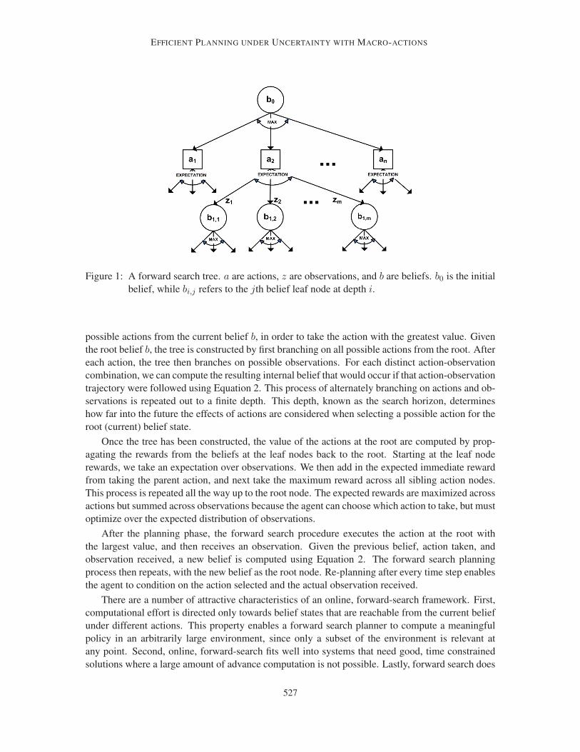
Figure 1: A forward search tree. a are actions, z are observations, and b are beliefs. b0 is the initial
belief, while bi,j refers to the jth belief leaf node at depth i.
possible actions from the current belief b, in order to take the action with the greatest value. Given
the root belief b, the tree is constructed by first branching on all possible actions from the root. After
each action, the tree then branches on possible observations. For each distinct action-observation
combination, we can compute the resulting internal belief that would occur if that action-observation
trajectory were followed using Equation 2. This process of alternately branching on actions and ob-
servations is repeated out to a finite depth. This depth, known as the search horizon, determines
how far into the future the effects of actions are considered when selecting a possible action for the
root (current) belief state.
Once the tree has been constructed, the value of the actions at the root are computed by prop-
agating the rewards from the beliefs at the leaf nodes back to the root. Starting at the leaf node
rewards, we take an expectation over observations. We then add in the expected immediate reward
from taking the parent action, and next take the maximum reward across all sibling action nodes.
This process is repeated all the way up to the root node. The expected rewards are maximized across
actions but summed across observations because the agent can choose which action to take, but must
optimize over the expected distribution of observations.
After the planning phase, the forward search procedure executes the action at the root with
the largest value, and then receives an observation. Given the previous belief, action taken, and
observation received, a new belief is computed using Equation 2. The forward search planning
process then repeats, with the new belief as the root node. Re-planning after every time step enables
the agent to condition on the action selected and the actual observation received.
There are a number of attractive characteristics of an online, forward-search framework. First,
computational effort is directed only towards belief states that are reachable from the current belief
under different actions. This property enables a forward search planner to compute a meaningful
policy in an arbitrarily large environment, since only a subset of the environment is relevant at
any point. Second, online, forward-search fits well into systems that need good, time constrained
solutions where a large amount of advance computation is not possible. Lastly, forward search does
527
HE, BRUNSKILL, & ROY
not have to compute an explicit representation of the value function, which can be an advantage in
factored domains where belief updating and immediate expected reward calculations are relatively
simple, but the value function itself is complex to represent.6
However, the computational cost of generic forward search will still scale with the cost of the be-
lief updating and immediate expected reward calculations, multiplied by the number of tree nodes
which grows exponentially with the search horizon. The costs of belief updating and calculating
the immediate expected reward typically scale either linearly or exponentially with the number of
state variables and the size of their respective domains, depending on the independence relations
among the state variables. When the state variables are continuously-valued, and therefore take
on an infinite number of values, we will typically need to employ some parametric or compressed
representation in order to make these calculations tractable. The number of tree nodes scales expo-
nentially with the horizon according toO((|A||Z|)H), where |A| and |Z| are the number of actions
and observations respectively and H is the search horizon. Therefore, standard forward search ap-
proaches will typically struggle when there are many state variables and/or state variables with large
domains and when a large H-step lookahead is necessary to achieve good performance.
One approach to accelerating planning over large, long horizon problems is to use temporally
extended macro-actions, a technique that has been used successfully in fully observable settings for
some years (Sutton, Precup, & Singh, 1999). There has been limited exploration of these ideas for
partially observable settings (exceptions include those by Theocharous & Kaelbling, 2003; Hsiao,
Lozano-Perez, & Kaelbling, 2008; Kurniawati, Du, Hsu, & Lee, 2009). In our work we define a
macro-action as a finite open-loop sequence of primitive actions that is executed without regard to
the observations received during the execution of this action sequence. For example, in our target
monitoring problem, one macro-action could be for the helicopter to travel to a key region, which
might involve a sequence of individual turns and straight line moves. By restricting the action space
to a set of length L macro-actions, the number of expanded nodes due to the action branching factor
can be reduced from|A|H to |A|H where A is the set of length L (or longer) macro-actions, and
H = HL is the macro-action horizon or depth7.
2.1 Macro-action Construction
If only a small set of macro-actions are evaluated during the search, the restricted action space will
result in significant computational savings due to the smaller exponent H (vs. H) in the compu-
tational complexity expression. However, this restriction can also result in poor algorithmic per-
formance if all the macro-actions being evaluated are unsuitable. In this paper, we assume that
macro-actions are provided by a domain expert as part of a comprehensive strategy to scaling up
to large problems with a multi-step lookahead. The macro-actions we use in our experimental re-
sults consist of open-loop policies which are a function of properties of the belief state at which
the macro-action is originated, and can be either computed and stored offline or computed online at
every timestep. Further details are provided in the experimental section.
Our reliance on domain knowledge in this paper is similar to prior work in the fully observable
community that separately investigated the potential advantage of macro-actions before turning to
6. An example of such a domain is one in which the state space is a set of independent variables, but the reward is an
aggregate function of these variables.
7. The macro-action depth refers to the number of macro-actions that are executed in sequence from the root belief node
to the leaves.
528

EFFICIENT PLANNING UNDER UNCERTAINTY WITH MACRO-ACTIONS
the challenge of learning these macro-actions (see the work by Sutton et al., 1999 for an overview of
one particular formalism). Although constructing macro-actions automatically is beyond the scope
of this paper, we have presented in related work a domain-independent algorithm (PUMA) that au-
tomatically generates macro-actions for planning in partially observable domains (He et al., 2010b).
Borrowing the notion of sub-goal states from the fully-observable planning literature (McGovern,
1998; Stolle & Precup, 2002), PUMA uses a heuristic that macro-actions can be designed to take
the agent, under the fully-observable model, from a possible start state under the current belief to
a sub-goal state. The PUMA algorithm was tested on variations of the experimental domains that
are used in this paper, and we encourage the reader to refer to the above-mentioned paper for more
details.
Regardless of how the set of macro-actions are generated, several key computational challenges
remain to scale macro-action forward-search to large, long environments. First, recall the number
of nodes in generic forward search scales as O(|A|H |Z|H). Using macro-actions reduces the first
term in the product, but does not directly change the second term, so the number of tree nodes still
is an exponential function of the search horizon H . Second, using macro-actions does not directly
alleviate the cost of performing belief updates and expected reward computations at each tree node,
and these computational costs can be substantial in large domains. The central contribution of our
paper is a method for efficiently and analytically computing the result of a macro-action given any
possible observation sequence received during its execution. This will allow us to use temporally-
extended actions to scale to certain types of large, long POMDPs.
3. The Posterior Belief Distribution Algorithm
To plan with macro-actions in a forward search manner, we must compute the expected reward re-
ceived during a macro-action, as well as the expected future value after taking that macro-action.
The reward the planner can expect to receive from a macro-action is the expected sum of the re-
wards under each of the posterior beliefs the agent will reach after each action in the macro-action.
However, the process is complicated by the fact that posterior the belief is also a result of receiving
an observation. As the agent does not know which observations will be received during the macro-
action, it cannot compute a single posterior belief reached during the macro-action, and therefore
cannot compute the expected reward.
Of course, an easy solution is to consider all possible observations, and compute the expected
reward of all possible beliefs that can result from all possible observations that could be received
during a macro-action. By computing the expected reward at each observation node, the AND-OR
tree constructed during forward search implicitly computes this expectation over all possible obser-
vation sequences. But, if computing the expected reward of a macro-action requires enumerating
all possible observation sequences that could be experienced during execution, the evaluation of a
macro-action will grow intractable quickly (see Figure 2(a)). The number of observation sequences
to be considered will grow exponentially with the length of the macro-action, and enumerating all
possible observations may not even be feasible in domains with continuous observations. One alter-
native may be to sample observation sequences for a given macro-action (Figure 2(b)), but sampling
is likely to still be computationally intensive due to the per-sample cost of performing a belief update
and expected reward calculation at each step of each sampled observation sequence.
We can avoid this computational burden by realizing that it is sometimes possible to analytically
represent the distribution over posterior beliefs. For a given sequence of actions, what we need is the
529
HE, BRUNSKILL, & ROY
(a) Exhaustive (b) Sampled (c) Analytic
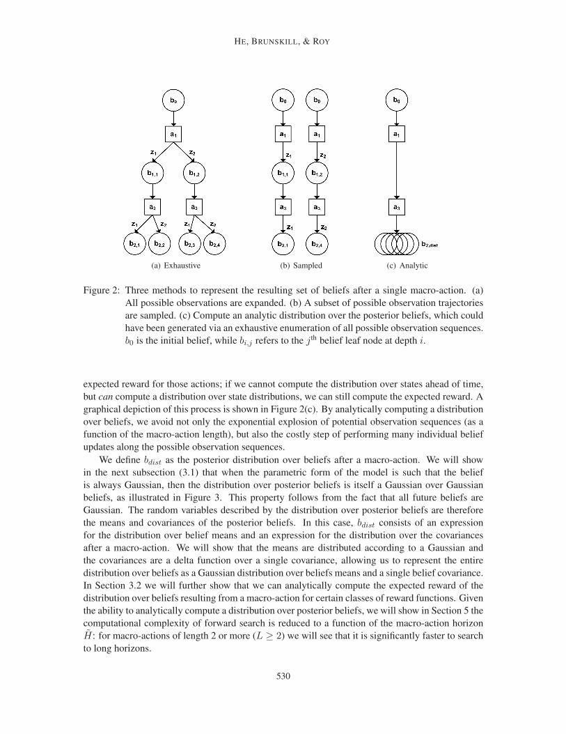
Figure 2: Three methods to represent the resulting set of beliefs after a single macro-action. (a)
All possible observations are expanded. (b) A subset of possible observation trajectories
are sampled. (c) Compute an analytic distribution over the posterior beliefs, which could
have been generated via an exhaustive enumeration of all possible observation sequences.
b0 is the initial belief, while bi,j refers to the jth belief leaf node at depth i.
expected reward for those actions; if we cannot compute the distribution over states ahead of time,
but can compute a distribution over state distributions, we can still compute the expected reward. A
graphical depiction of this process is shown in Figure 2(c). By analytically computing a distribution
over beliefs, we avoid not only the exponential explosion of potential observation sequences (as a
function of the macro-action length), but also the costly step of performing many individual belief
updates along the possible observation sequences.
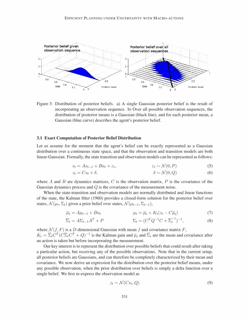
We define bdist as the posterior distribution over beliefs after a macro-action. We will show
in the next subsection (3.1) that when the parametric form of the model is such that the belief
is always Gaussian, then the distribution over posterior beliefs is itself a Gaussian over Gaussian
beliefs, as illustrated in Figure 3. This property follows from the fact that all future beliefs are
Gaussian. The random variables described by the distribution over posterior beliefs are therefore
the means and covariances of the posterior beliefs. In this case, bdist consists of an expression
for the distribution over belief means and an expression for the distribution over the covariances
after a macro-action. We will show that the means are distributed according to a Gaussian and
the covariances are a delta function over a single covariance, allowing us to represent the entire
distribution over beliefs as a Gaussian distribution over beliefs means and a single belief covariance.
In Section 3.2 we will further show that we can analytically compute the expected reward of the
distribution over beliefs resulting from a macro-action for certain classes of reward functions. Given
the ability to analytically compute a distribution over posterior beliefs, we will show in Section 5 the
computational complexity of forward search is reduced to a function of the macro-action horizon
H: for macro-actions of length 2 or more (L ≥ 2) we will see that it is significantly faster to search
to long horizons.
530
EFFICIENT PLANNING UNDER UNCERTAINTY WITH MACRO-ACTIONS
Figure 3: Distribution of posterior beliefs. a) A single Gaussian posterior belief is the result of
incorporating an observation sequence. b) Over all possible observation sequences, the
distribution of posterior means is a Gaussian (black line), and for each posterior mean, a
Gaussian (blue curve) describes the agent’s posterior belief.
3.1 Exact Computation of Posterior Belief Distribution
Let us assume for the moment that the agent’s belief can be exactly represented as a Gaussian
distribution over a continuous state space, and that the observation and transition models are both
linear-Gaussian. Formally, the state transition and observation models can be represented as follows:
st = Ast−1 + Bat + εt, εt ∼ N (0, P ) (5)
zt = Cst + δ, δ ∼ N (0, Q) (6)
where A and B are dynamics matrices, C is the observation matrix, P is the covariance of the
Gaussian dynamics process and Q is the covariance of the measurement noise.
When the state-transition and observation models are normally distributed and linear functions
of the state, the Kalman filter (1960) provides a closed-form solution for the posterior belief over
states, N (µt, Σt) given a prior belief over states, N (µt−1, Σt−1),
µt = Aµt−1 + Bat µt = µt + Kt(zt − Cµt) (7)
Σt = AΣt−1AT + P Σt = (CT Q−1C + Σ
−1t )−1, (8)
where N (f, F ) is a D-dimensional Gaussian with mean f and covariance matrix F ,
Kt = ΣtCT (CΣtC
T + Q)−1 is the Kalman gain and µt and Σt are the mean and covariance after
an action is taken but before incorporating the measurement.
Our key interest is to represent the distribution over possible beliefs that could result after taking
a particular action, but receiving any of the possible observations. Note that in the current setup,
all posterior beliefs are Gaussians, and can therefore be completely characterized by their mean and
covariance. We now derive an expression for the distribution over the posterior belief means, under
any possible observation, when the prior distribution over beliefs is simply a delta function over a
single belief. We first re-express the observation model as
zt ∼ N (Cst, Q) (9)
531

HE, BRUNSKILL, & ROY
which we can use to compute an expression for the probability of an observation given the belief
mean, p(zt|µt), by marginalizing over st ∼ N (µt, Σt), as
p(zt|µt) =∫
p(zt|st)p(st|µt)dst (10)
= N (Cµt, CΣtCT + Q). (11)
We can perform further linear transformations to obtain an expression for the distribution of poste-
rior means, under any potential observation:
zt ∼ N (Cµt, CΣtCT + Q) (12)
zt − Cµt ∼ N (0, CΣtCT + Q) (13)
Kt(zt − Cµt) ∼ N (0, Kt(CΣtCT + Q)KT
t ) (14)
µt + Kt(zt − Cµt) ∼ N (µt, Kt(CΣtCT + Q)KT
t ) (15)
µt ∼ N (µt, Kt(CΣtCT + Q)KT
t ) (16)
µt ∼ N (µt, ΣtCT KT
t ) (17)
where Equation 17 is computed by substituting the definition of the Kalman gain.
At this point, a somewhat unusual change has occurred, in that µt, the mean of the distribution
itself, is now a random variable. Without knowing the value of the particular observation that
occurs after a primitive action, we cannot deterministically predict the posterior mean of the belief.8
However, we can model the probability of any specific belief state, which effectively means that
we will compute a distribution over the belief means µ and covariances Σ. Equation 17 shows
that the distribution over the belief means is normally distributed about µt, with a covariance that
depends on the prior covariance Σt and the observation model parameters. Sampling a mean from
this distribution is equivalent to selecting a particular observation.
We have just presented a formula for calculating the posterior distribution over belief means
after one action, and any possible observation. We now wish to show that the posterior distribution
over beliefs means after a sequence of actions remains a Gaussian distribution. This will allow us
to compute an analytic expression for the posterior distribution over beliefs that could result from
a macro-action. We therefore require a method to iteratively use Equation 17 in order to compute
the posterior distribution over beliefs for a complete macro-action and any possible observation
sequence.
We first combine the process and measurement updates for a single primitive action belief up-
date in order to get an expression for the posterior belief means in terms of the prior belief mean.
We marginalize over µt, the posterior belief after the transition update but before the observation
update, using p(µt|µt−1) =∫
p(µt|µt)p(µt|µt−1)dµt. As µt is a deterministic function of µt−1 (see
Equation 7a), then p(µt|µt−1) is simply a delta function, which means that p(µt|µt−1) is identical
to Equation 17 after substituting µt using Equation 7a:
p(µt|µt−1) = N (Aµt−1 + Bat, ΣtCT KT
t ). (18)
In a one-step belief update, the belief mean at the prior time step, µt−1, is assumed to be a known
value. However, for a macro-action, once the first primitive action has been taken, the posterior be-
8. Note that we will show later in this section that we can deterministically predict the posterior belief covariance. Its
distribution is a Dirac delta that is independent of the specific observation received.
532
EFFICIENT PLANNING UNDER UNCERTAINTY WITH MACRO-ACTIONS
lief mean will depend on the received observation. In absence of the knowledge of that received ob-
servation, we will instead have a distribution over the belief means. Therefore, for the second prim-
itive action in the macro-action, the prior belief is now given as a Gaussian µt−1 ∼ N (mt−1, Σµt−1)
where mt−1 and Σµt−1 are random variables. In order to compute the probability distribution over
µt, we must integrate over this distribution of prior belief means µt−1:
p(µt|mt−1, Σµt−1) =
∫
µt−1
p(µt|µt−1)p(µt−1|mt−1, Σµt−1)dµt−1. (19)
Since both terms inside the integral are Gaussian distributions, we can analytically combine these
two Gaussians, one of which is independent of µt−1 and one of which is dependent on µt−1. Inte-
grating over µt−1, as we had done in Equations 9-11, we find that the mean of the posterior belief
means is conveniently still a Gaussian distribution over a function of the prior mean of the belief
means and covariance:
µt ∼ N (Amt−1 + Bat, AΣµt−1A
T + ΣtCT KT
t ) (20)
or
µt ∼ N (mt, Σµt ) (21)
where mt = Amt−1 + Bat and Σµt = AΣµ
t−1AT + ΣtC
T KTt . Equation 20 can now be used to
predict the posterior mean distribution after a multi-step action sequence. Assuming that the agent
is currently at time t and has a particular prior mean µt (which we can also express as a Gaussian
with zero covariance, N (µt, 0)), the posterior mean after an action sequence of D time steps is
distributed as follows:
µt+D ∼ N (mt+D, Σµt:t+D) (22)
where
mt+D = f(µt−1, A, B, at+1:t+D) (23)
= A mt+D−1 + B at+D (24)
= ADmt +D∑
i=1
AD−iBat+i, (25)
and
Σµt:t+D =
t+D∑
i=t
At+D−iΣiCTi DT
i (At+D−i)T . (26)
Note that mt+D does not depend on observations; it gives the mean of the distribution of beliefs that
might result from the received observations. mt+D is dependent only on the state-transition model
parameters and can be calculated via a recursive update along the action sequence.
We now consider the covariance of the posterior beliefs that may result after taking a macro-
action. Recall that for a single belief, the posterior covariance after taking a primitive action and
receiving a particular observation can be calculated using Equation 8. Note that this formula is inde-
pendent of the actual received observation zt, and the prior µt−1 or posterior mean µt. Formally, this
533
HE, BRUNSKILL, & ROY
property exists because the Fisher information associated with the observation model is independent
of the specific observations. Therefore, the posterior covariance after any observation sequence of
known length can be calculated in closed form given the prior covariance, without needing to know
the observations received along the way.
We can now specify the form of bdist, the posterior distribution over beliefs after a macro-action:
bdist(µt+T , Σ) = N (f(µt−1, A, B, at:t+T ), Σµt:T ) · δ(Σ, Σ′) (27)
where bdist(µt+T , Σ) is the probability of arriving in posterior belief b = N (µt+T , Σ) after taking a
particular macro-action, Equation 22 defines the distribution over belief means, and Σ′ is computed
by iteratively applying Equation 8. This expression shows that for problems with linear-Gaussian
state-transition and observation models, we can exactly calculate the distribution of posterior beliefs
associated with a macro-action.
3.2 Calculating the Expected Reward
The prior section outlined a procedure for calculating the posterior set of beliefs after a macro-
action. The reason to compute this distribution is in turn to be able to calculate the expected reward
of each macro-action, which will be used to compute the best action for the current belief.
To calculate the expected reward of a macro-action, we start by considering the expected reward
of starting in a particular belief state b0 and executing a L-length macro-action a consisting of
actions a1, a2, . . . , aL. This may be expressed as
r(b0, a1:L) = r(b0, a1) + γ
∫
z1
p(z1|b0, a)Q(ba1,z1 , a2:L) (28)
where we have used ba1,z1 to represent the updated belief after taking action a1 and receiving obser-
vation z1 from b0, a2:L to represent the macro-action consisting of the second through L-th primitive
actions of the macro-action a, and Q(ba1,z1 , a2:L) to represent the future expected reward of taking
the remaining actions from belief ba1,z1 . Recursively expanding the second term in Equation 28 we
obtain the following expression
r(b0, a1:L) = r(b0, a1) + γ
∫
z1
p(z1|b0, a1)r(ba1,z1 , a2) +
γ2
∫
z1,z2
p(z1|b0, a1)p(z2|ba1,z1 , a2)r(ba1,z1,a2,z2 , a3) + · · · (29)
γL−1
∫
z1,...,zL
[
L−1∏
i=1
p(zi|ba1,z1,...,ai−1,zi−1 , ai)
]
r(ba1,...aL−1,zL−1 , aL). (30)
The first term in Equation 29 represents the expected reward from taking the first primitive action
in the macro-action from the initial belief state. The remaining terms each represent the expected
reward at the i-th primitive action of the macro-action, where the expectation is taken over all
possible i − 1 length sequences of observations that could have been received up to that point (as
well as the standard integration over the state space). From Equation 27 we have a closed form
expression for the distribution over belief states possible after a sequence of primitive actions. We
can use this to re-express Equation 29 as a function of the distributions over beliefs:
r(b0, a1:L) = r(b0, a1) +L∑
i=2
γi−1r(bi−1dist, ai) (31)
534

EFFICIENT PLANNING UNDER UNCERTAINTY WITH MACRO-ACTIONS
where bi−1dist is used to represent the posterior distribution over beliefs that results after taking the
first i − 1 primitive actions in macro action a. Slightly abusing notation, r(bdist, ai) represents
the expected reward for taking action ai given the posterior distribution over beliefs bdist, and is
expressed as
r(bdist, ai) =
∫
b
∫
sb(s)bdist(b)r(s, ai)dsdb. (32)
Combining Equations 31 and 32, we can see that the expected reward of a macro-action can be
calculated from the sum of the expected reward of taking a primitive action from the posterior
distribution of beliefs at each step along the macro-action.
Recall from the prior section that the posterior distribution over beliefs can be factored into a
Gaussian distribution over the belief means µ (Equation 22), and a Dirac delta distribution over the
belief covariances Σ (since all beliefs will have identical covariances):
bdist(µ,Σ) = N (µ|ma, Σµa)δ(Σ, Σa) (33)
where ma is the mean of the belief means after primitive action a, Σµa is the covariance of the belief
means after primitive action a, and Σa is the covariance of a belief state after primitive action a.
As the belief state itself is a Gaussian,
b(s) = N (s|µ,Σ), (34)
we can re-express the reward as
r(bdist, a) =
∫
s
∫
µ,Σr(s, a)N (s|µ,Σ)N (µ|ma, Σ
µa)δ(Σ, Σa)dsdµdΣ (35)
=
∫
s
∫
µr(s, a)N (s|µ,Σa)N (µ|ma, Σ
µa)dµds, (36)
where the second line follows due to the Dirac delta distribution on the belief covariances. Expand-
ing out the formula for N (s|µ,Σ) we see it is identical to the formula for N (µ|s,Σ):
N (s|µ,Σ) =1√
2π|Σ|Nd/2exp(−1
2(s− µ)Σ−1(s− µ)T ) (37)
=1√
2π|Σ|Nd/2exp(−1
2(µ− s)Σ−1(µ− s)T ) (38)
= N (µ|s,Σ). (39)
Therefore, we can substitute the equivalent expression to yield
r(bdist, a) =
∫
s
∫
µr(s, a)N (µ|s,Σa)N (µ|ma, Σ
µa)dµds. (40)
Completing the square in the exponent, we re-express the product of the above two Gaussians as
r(bdist, a) =
∫
s
∫
µr(s, a)N (s|ma, Σa + Σµ
a)N (µ|c, C)dµds, (41)
535
HE, BRUNSKILL, & ROY
where C = (Σ−1a + (Σµ
a)−1)−1 and c = C(ma(Σµa)−1 + µΣ−1
a ). We then integrate over µ to get
r(bdist, a) =
∫
sr(s, a)N (s|ma, Σa + Σµ
a)ds. (42)
If the reward model itself is a weighted sum of Nr Gaussians,
r(s, a) =
Nr∑
j=1
wjN (s|ζj , Υj), (43)
then the integral in Equation 42 can be evaluated in closed form as
r(bdist, a) =
∫
s
Nr∑
j=1
wjN (s|ζj , Υj)N (s|ma, Σa + Σµa)ds (44)
=
Nr∑
j=1
wjN (ζj |ma, Υj + Σa + Σµa)
∫
sN (s|c1, C1), (45)
where we have again completed the square in the exponent, and defined new constants C1 = (Υ−1j +
(Σa + Σµa)−1)−1 and c1 = C1(ζjΥ
−1j + ma(Σa + Σµ
a)−1). Integrating we obtain an analytic
expression for the expected reward of a primitive action under a distribution of beliefs:
r(bdist, a) =
Nr∑
j=1
wjN (ζj |ma, Υj + Σa + Σµa). (46)
A similar closed-form expression is available if the reward model is a polynomial function of
the state,
r(s, a) =
Nr∑
j=1
wjsj , (47)
instead of a weighted sum of Gaussians. Substituting Equation 47 into Equation 42 yields
r(bdist, a) =
∫
s
Nr∑
j=1
wjsjN (s|ma, Σa + Σµ
a)ds
=
Nr∑
j=1
wj
∫
ssjN (s|ma, Σa + Σµ
a)ds. (48)
Therefore, evaluating the expected reward involves calculating the first Nr moments of a Gaussian
distribution. Each of these moments is an analytic expression of the Gaussian mean and covari-
ance.9 So, for reward models that are either a weighted sum of Gaussians, or which are polynomial
functions of the state space, the expected reward of a macro-action (Equation 28) can be computed
analytically.
For other arbitrary reward models it may not be possible to analytically compute the expected
reward of taking a primitive action in a particular distribution over beliefs. In such cases, we can
approximate the expectation in Equation 42 by sampling.
9. The Gaussian distribution is completely described by its first two moments; all higher order moments are simply
functions of the first two moments.
536
EFFICIENT PLANNING UNDER UNCERTAINTY WITH MACRO-ACTIONS
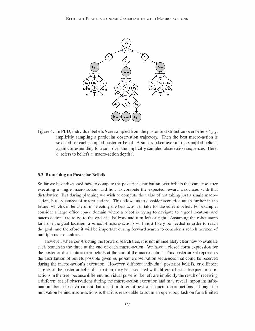
Figure 4: In PBD, individual beliefs b are sampled from the posterior distribution over beliefs bdist,
implicitly sampling a particular observation trajectory. Then the best macro-action is
selected for each sampled posterior belief. A sum is taken over all the sampled beliefs,
again corresponding to a sum over the implicitly sampled observation sequences. Here,
bi refers to beliefs at macro-action depth i.
3.3 Branching on Posterior Beliefs
So far we have discussed how to compute the posterior distribution over beliefs that can arise after
executing a single macro-action, and how to compute the expected reward associated with that
distribution. But during planning we wish to compute the value of not taking just a single macro-
action, but sequences of macro-actions. This allows us to consider scenarios much further in the
future, which can be useful in selecting the best action to take for the current belief. For example,
consider a large office space domain where a robot is trying to navigate to a goal location, and
macro-actions are to go to the end of a hallway and turn left or right. Assuming the robot starts
far from the goal location, a series of macro-actions will most likely be needed in order to reach
the goal, and therefore it will be important during forward search to consider a search horizon of
multiple macro-actions.
However, when constructing the forward search tree, it is not immediately clear how to evaluate
each branch in the three at the end of each macro-action. We have a closed form expression for
the posterior distribution over beliefs at the end of the macro-action. This posterior set represents
the distribution of beliefs possible given all possible observation sequences that could be received
during the macro-action’s execution. However, different individual posterior beliefs, or different
subsets of the posterior belief distribution, may be associated with different best subsequent macro-
actions in the tree, because different individual posterior beliefs are implicitly the result of receiving
a different set of observations during the macro-action execution and may reveal important infor-
mation about the environment that result in different best subsequent macro-actions. Though the
motivation behind macro-actions is that it is reasonable to act in an open-loop fashion for a limited
537
HE, BRUNSKILL, & ROY
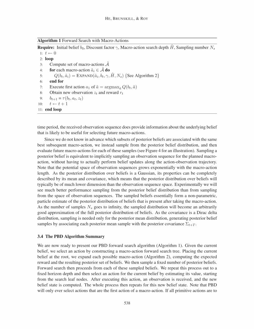
Algorithm 1 Forward Search with Macro-Actions
Require: Initial belief b0, Discount factor γ, Macro-action search depth H , Sampling number Ns
1: t← 02: loop
3: Compute set of macro-actions A4: for each macro-action ai ∈ A do
5: Q(bt, ai) = EXPAND(ai, bt, γ, H, Ns) {See Algorithm 2}6: end for
7: Execute first action a1 of a = argmaxa Q(bt, a)8: Obtain new observation zt and reward rt
9: bt+1 = τ(bt, at, zt)10: t← t + 111: end loop
time period, the received observation sequence does provide information about the underlying belief
that is likely to be useful for selecting future macro-actions.
Since we do not know in advance which subsets of posterior beliefs are associated with the same
best subsequent macro-action, we instead sample from the posterior belief distribution, and then
evaluate future macro-actions for each of these samples (see Figure 4 for an illustration). Sampling a
posterior belief is equivalent to implicitly sampling an observation sequence for the planned macro-
action, without having to actually perform belief updates along the action-observation trajectory.
Note that the potential space of observation sequences grows exponentially with the macro-action
length. As the posterior distribution over beliefs is a Gaussian, its properties can be completely
described by its mean and covariance, which means that the posterior distribution over beliefs will
typically be of much lower dimension than the observation sequence space. Experimentally we will
see much better performance sampling from the posterior belief distribution than from sampling
from the space of observation sequences. The sampled beliefs essentially form a non-parametric,
particle estimate of the posterior distribution of beliefs that is present after taking the macro-action.
As the number of samples Ns goes to infinity, the sampled distribution will become an arbitrarily
good approximation of the full posterior distribution of beliefs. As the covariance is a Dirac delta
distribution, sampling is needed only for the posterior mean distribution, generating posterior belief
samples by associating each posterior mean sample with the posterior covariance Σt+T .
3.4 The PBD Algorithm Summary
We are now ready to present our PBD forward search algorithm (Algorithm 1). Given the current
belief, we select an action by constructing a macro-action forward search tree. Placing the current
belief at the root, we expand each possible macro-action (Algorithm 2), computing the expected
reward and the resulting posterior set of beliefs. We then sample a fixed number of posterior beliefs.
Forward search then proceeds from each of these sampled beliefs. We repeat this process out to a
fixed horizon depth and then select an action for the current belief by estimating its value, starting
from the search leaf nodes. After executing this action, an observation is received, and the new
belief state is computed. The whole process then repeats for this new belief state. Note that PBD
will only ever select actions that are the first action of a macro-action. If all primitive actions are to
538

EFFICIENT PLANNING UNDER UNCERTAINTY WITH MACRO-ACTIONS
Algorithm 2 EXPAND – Expand Macro-actions via PBD
1: Input: Macro-action a, Belief state bt, Discount factor γ, Macro-action search depth H ,
No. posterior belief samples per macro-action Ns
2: if H = 0 then
3: return 0
4: else {Expand Macro-action a={a1, . . . , aL}}5: Ra = 06: bdist = bt
7: for j = 1 to L do
8: Ra = Ra + γ ∗ r(bdist, aj)9: Update the posterior distribution of beliefs bdist
10: end for
11: for i = 1 to Ns do
12: Sample posterior mean ni according to N (mt+T , Σµt+T )
13: bi ← N (ni, Σt+T )14: Generate next set of macro-actions Anext
15: for anexti ∈ Anext do
16: Q(bi, anexti ) = EXPAND(anext
i ,bi,γ,H − 1,Ns)
17: end for
18: V = Ra + 1Ns
γL maxanexti
Q(bi, anexti ))
19: end for
20: return V21: end if
be considered, the number of macro-actions that are evaluated for the root belief at every timestep
must be at least the same as the size of the primitive action space, and each primitive action must be
the first action of at least one macro-action.
4. Approximate Computation of Posterior Belief Distributions
The PBD algorithm described so far assumes that the transition and observation functions are lin-
ear functions of the state with Gaussian noise. When these functions are non-linear, the traditional
Kalman filter model no longer provides an exact belief update, and for the PBD algorithm, the dis-
tribution of posterior beliefs cannot be calculated exactly. In this section we briefly describe an
extension to the PBD algorithm to handle a wider class of observation models, namely paramet-
ric models that are members of the exponential family of distributions (Barndorff-Nielsen, 1979).
For non-linear transition models, there exist techniques such as the extended Kalman filter to ap-
proximate the posterior with a Gaussian; however, we do not formally consider incorporating such
techniques into our PBD algorithm here.
We choose to consider exponential family observation models since this family includes a wide
array of distributions, such as Gaussian, Bernoulli, and Poisson distributions, and has certain appeal-
ing mathematical properties. In particular, we leverage work by West, Harrison and Migon (1985)
who constructed linear-Gaussian models that approximate the non-Gaussian exponential family ob-
servation model in the neighborhood of the conditional mode, st|zt. They then used the approximate
539
HE, BRUNSKILL, & ROY
linear-Gaussian observation mode in a traditional Kalman filter, to maintain a closed-form Gaussian
representation of the posterior belief, creating an exponential family Kalman Filter (efKF). For com-
pleteness we include West et al.’s derivation of the filter in Appendix A, and we present the main
equations here.
Constructing the approximate linear-Gaussian observation model requires computation of the
first two moments of the distribution and the linearization around the mean estimate at every time
step. An exponential family observation model can be represented as follows,
p(zt|θt) = exp(zTt θt − βt(θt) + κt(zt)), θt = W (st) (49)
where st is the hidden state of the system, θt and βt(θt) are the canonical parameter and normal-
ization factor of the distribution, and W (.) maps the states to canonical parameter values. W (.) is
also known as the canonical link function, and depends on the particular member of the exponential
family.
The first two moments of the distribution (West et al., 1985) are
E(zt|θt) = βt =∂βt(θt)
∂θt
∣
∣
∣
θt=W (µt)V ar(zt|θt) = βt =
∂2βt(θt)
∂θt∂θTt
∣
∣
∣
θt=W (µt)(50)
where βt and βt are the derivatives of the exponential family distribution’s normalization factor,
both linearized about θt = W (µt).Given an action-observation sequence, the posterior mean of the agent’s belief in the efKF can
then be updated according to
µt = Aµt−1 + Bat µt = µt + Kt(zt −W (µt)), (51)
Σt = AΣt−1AT + P Σt = (Σ
−1t + Y T
t βtYt)−1, (52)
where Kt = ΣtYt(YtΣtYTt + β−1
t )−1 is the efKF Kalman gain, and zt = θt − β−1t · (βt − zt)
is the projection of the observation onto the parameter space of the exponential family observation
model. Yt = ∂θt
∂st
∣
∣
st=µtis the gradient of the exponential family distribution’s canonical parameter,
linearized about µt.
We can now incorporate these results to compute a modified form for the posterior belief mean
and covariance distributions, which were represented by Equations 8 and 22 when the observation
model was linear Gaussian. Now, for exponential family observation models, the posterior belief
covariance comes from Equation 52. The expression for the distribution of the posterior means can
be modified based on the efKF equations:
µt+T ∼ N (f(µt−1, At:t+T , Bt:t+T , at:t+T ),t+T∑
i=t
ΣiYTi KT
i ). (53)
It is worth noting that in contrast to our prior expressions for the posterior belief distribution
(Equations 8 and 22), which are exact and completely independent of the received observations,
Equations 52 and 53 are no longer independent of the observations obtained because the obser-
vation model parameters are linearized about the prior mean µt. Hence while the parameters are
independent of the observation that will be obtained for a macro-action sequence of length 1, for a
540

EFFICIENT PLANNING UNDER UNCERTAINTY WITH MACRO-ACTIONS
longer macro-action, the observation model parameters depend on the prior observations obtained.
We approximate this update by linearizing about the mean of the prior mean distribution mt at each
step along the action sequence, rather than the true prior belief mean µt. We will shortly see that we
still obtain good experimental results using this approximation.
An alternate popular approach for non-Gaussian systems is to use a particle filter to represent the
system state. However, in high dimensional, continuous environments similar to the ones considered
in this paper, particle filters often suffer from particle depletion, or require a very large number of
particles to accurately capture the posterior. The costs of belief updating and expected reward
calculations scale with the number of particles. In contrast, our approximate PBD computation has
the same computational complexity as our exact PBD computation, which we will demonstrate in
later sections to scale polynomially with the number of state dimensions.
This approximate method for computing the posterior distribution over beliefs can be used as a
substitute for exactly calculating the posterior distribution over beliefs in the PBD algorithm.
5. Analysis
Here we provide a formal analysis of the accuracy and computational complexity of our PBD al-
gorithm. Throughout this section we assume belief states can be represented exactly as Gaussian
distributions: in other words, we assume a linear-Gaussian system. In the following sections we
will demonstrate experimentally that the PBD algorithm is useful in a wider variety of problems
using an EKF or the efKF described in Section 4, but incorporating the error of these approximate
filtering techniques into an analysis of the algorithm is a topic for future research.
5.1 Performance
PBD selects actions by performing a limited-horizon forward search using a restricted policy space
induced by the macro-actions. However, during execution, only the first step of the macro-action
is taken. After an observation is received, the belief state is updated, and then planning is repeated
from the resulting belief. By only taking the first primitive action, the system may take sequences
of actions that do not correspond to any of the known macro-actions, effectively expanding the
considered policy space. As a result, the performance will be at least as good as actually executing
the entire macro-action. However, it would be useful to determine if any claims can be made about
the belief-action values calculated as part of the PBD algorithm. Obviously, the received rewards
of the executed policy will always be less than or equal to the optimal policy’s rewards, since the
policy space considered during planning is smaller than the full policy space. However, the values
calculated by the PBD algorithm are only approximate values due to the approximations (such as
sampling a subset of the posterior beliefs) made during the computation process. We now prove that
for linear-Gaussian systems, the values computed by PBD, minus an additional epsilon term due to
the approximations incurred by sampling a subset of the posterior beliefs after each macro-action,
are probabilistically guaranteed to be a lower bound on the true optimal values. For the purpose of
this analysis we will assume that all rewards are scaled to lie between 0 and 1. M is the maximum
number of macro-actions.
Theorem 5.1 Given a linear-Gaussian system, an initial belief b, and any δ > 0, and for any
reward model which is either a weighted sum of Gaussians, or a polynomial function, the following
541
HE, BRUNSKILL, & ROY
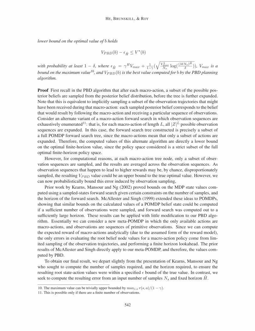
lower bound on the optimal value of b holds
VPBD(b)− ǫH ≤ V ∗(b)
with probability at least 1 − δ, where ǫH = γHVmax + 11−γ (
√
V 2max
Nslog( (MNs)H
δ )), Vmax is a
bound on the maximum value10, and VPBD(b) is the best value computed for b by the PBD planning
algorithm.
Proof First recall in the PBD algorithm that after each macro-action, a subset of the possible pos-
terior beliefs are sampled from the posterior belief distribution, before the tree is further expanded.
Note that this is equivalent to implicitly sampling a subset of the observation trajectories that might
have been received during that macro-action: each sampled posterior belief corresponds to the belief
that would result by following the macro-action and receiving a particular sequence of observations.
Consider an alternate variant of a macro-action forward search in which observation sequences are
exhaustively enumerated11: that is, for each macro-action of length L, all |Z|L possible observation
sequences are expanded. In this case, the forward search tree constructed is precisely a subset of
a full POMDP forward search tree, since the macro-actions mean that only a subset of actions are
expanded. Therefore, the computed values of this alternate algorithm are directly a lower bound
on the optimal finite-horizon value, since the policy space considered is a strict subset of the full
optimal finite-horizon policy space.
However, for computational reasons, at each macro-action tree node, only a subset of obser-
vation sequences are sampled, and the results are averaged across the observation sequences. As
observation sequences that happen to lead to higher rewards may be, by chance, disproportionately
sampled, the resulting VPBD value could be an upper bound to the true optimal value. However, we
can now probabilistically bound this error induced by observation sampling,
Prior work by Kearns, Mansour and Ng (2002) proved bounds on the MDP state values com-
puted using a sampled-states forward search given certain constraints on the number of samples, and
the horizon of the forward search. McAllester and Singh (1999) extended these ideas to POMDPs,
showing that similar bounds on the calculated values of a POMDP belief state could be computed
if a sufficient number of observations were sampled, and forward search was computed out to a
sufficiently large horizon. These results can be applied with little modification to our PBD algo-
rithm. Essentially we can consider a new meta-POMDP in which the only available actions are
macro-actions, and observations are sequences of primitive observations. Since we can compute
the expected reward of macro-actions analytically (due to the assumed form of the reward model),
the only errors in evaluating the root belief node values for a macro-action policy come from lim-
ited sampling of the observation trajectories, and performing a finite horizon lookahead. The prior
results of McAllester and Singh directly apply to our meta-POMDP, and therefore, the values com-
puted by PBD.
To obtain our final result, we depart slightly from the presentation of Kearns, Mansour and Ng
who sought to compute the number of samples required, and the horizon required, to ensure the
resulting root state-action values were within a specified ǫ bound of the true value. In contrast, we
seek to compute the resulting error from an input number of samples Ns and fixed horizon H .
10. The maximum value can be trivially upper bounded by maxs,a r(s, a)/(1 − γ).
11. This is possible only if there are a finite number of observations.
542

EFFICIENT PLANNING UNDER UNCERTAINTY WITH MACRO-ACTIONS
In the proof of Kearns, Mansour and Ng, they show that the error between the calculated H-
horizon state-action value QH(b, a) and the true infinite-horizon policy value Q(b, a) is
|QH(b, a)−Q(b, a)| ≤ γHVmax +ǫ
1− γ(54)
with probability at least 1− δ if
δ ≥ (MNs)Hexp(−ǫ2Ns/V 2
max). (55)
We can solve Equation 55 for ǫ, to yield
ǫ ≤
√
V 2max
Nslog((MNs)H
δ
)
. (56)
Substituting Equation 56 into Equation 54 and re-arranging yields the desired result.
If the reward of a macro-action cannot be analytically computed, we can approximate its value
by sampling Nr samples at each primitive action along the length-L macro-action. For an input
δ′ we can compute a probabilistic bound on the resulting error of the approximate value at each
primitive action using Chernoff’s bound. Using the union bound, the probability that the true error
will exceed this threshold at any primitive action along the macro-action is no more than Lδ′, and
the resulting error is at most the sum of the error at each primitive action. This error (and probability
of error) can be easily incorporated to extend Theorem 1 to the case of generic reward models.
Note that Theorem 1 only states that with high probability that VPBD − ǫH is a lower bound
on the optimal value: it does not provide a tight bound on how close the computed VPBD is to
the optimal value. To state this in an alternate way, ǫH provides a bound on the error introduced
by sampling observation sequences, but PBD still is designed to only search over a limited policy
space, that defined by the macro-actions chosen and used in the forward search. Therefore in general
the computed values, even when a large number of observation sequences are sampled, may be
substantially less than the value under the optimal policy.
5.2 Computational Complexity
One of the central contributions of our work is providing an efficient macro-action forward search
algorithm that can scale to long horizons and large problems. We now analyze the computational
complexity of our approach. The computational cost will be a function of two operations: comput-
ing the posterior distribution over beliefs, and computing the expected reward of a distribution over
beliefs. As we will shortly see, the computational complexity of these operations is a polynomial
function of the state space dimension.12 This low order relationship is possible due to the particu-
lar parametric representation employed for the posterior distribution over beliefs: representing the
posterior distribution over beliefs as a Gaussian requires a number of parameters that scales only
quadratically with the number of state dimensions.13 PBD is therefore able to scale to large do-
mains. Our computational complexity results are summarized in Table 1. Throughout this analysis
12. If there are multiple independent state variables, or factors, the complexity increases linearly with the number of
independent factors.
13. To represent a Gaussian in X dimensions requires an X-dimensional vector to specify the mean, and O(X2) param-
eters to specify the covariance.
543

HE, BRUNSKILL, & ROY
we presume that the macro-actions themselves were selected or computed in advance; in general,
the cost of computing domain-relevant macro-actions will depend on the particular domain, and
we do not here analyze the possible additional computational cost incurred during macro-action
construction.
5.2.1 COMPLEXITY OF GAUSSIAN BELIEF UPDATING FOR A LENGTH L MACRO-ACTION
The computation for the posterior distribution over beliefs resulting from a macro-action was pre-
sented in Equation 53, and consists of a set of matrix multiplications and inversions. Matrix mul-
tiplication is an O(D2) computation, where D is the state space dimension. Matrix inversion can
be done in O(D3) time. Therefore the computational cost of performing a single update of the pos-
terior over belief states is an O(D3) operation. This update must be performed for each primitive
action in a length-L macro-action a, resulting in a computational cost of
O(LD3) (57)
for a single macro-action.
In Section 4 we presented a set of equations (Equations 50- 53) that we use to approximately
compute the posterior distribution over beliefs when the observation model is not Gaussian, but is
an exponential family. These equations again consist of a set of matrix multiplications, and the cost
of a single update, and cost of updating over a length-L macro-action will again be O(D3) and
O(LD3), respectively.14
5.2.2 COMPLEXITY OF ANALYTICALLY COMPUTING THE EXPECTED REWARD OF A LENGTH
L MACRO-ACTION
The second component of the computational cost comes when we evaluate the expected reward of
a macro-action. If the reward is a weighted sum of Nr Gaussians, as specified by Equation 43,
this operation involves evaluating the value of NrL Gaussians at particular fixed points. Evaluating
a D-dimensional Gaussian at a single point is an O(D3) operation, due to the inverse covariance
that must be computed. The cost for performing this operation NrL times is simply O(NrLD3).Therefore the total cost for evaluating the expected reward of a macro-action when the reward model
is a weighted sum of Nr Gaussians is:
O(LD3(Nr + 1)). (58)
If instead the reward model is a Nr-th degree polynomial function of the state, then the expected
reward calculation consists of the cost of calculating the Nr-moments of a D-dimensional Gaussian
distribution (Equation 48). Assume without loss of generality that we are computing the Nr-th
central moment of a D-dimensional Gaussian: a non-central moment can always be converted into
a central moment by adding and subtracting a mean term. Let the Nr-th central moment denote
moments of the form E[(s1 − E[s1])2(s2 − E[s2]) . . . (sD − E[sD])] or E[(s2 − E[s2])
Nr ], and
σij denote the ij-th entry of the covariance matrix. From the work by Triantafyllopoulos (2003) we
know that if Nr is odd, the central Nr-th moments are zero, and if Nr is even (Nr = 2k) any Nr-th
14. The actual computational cost will be higher for the efKF filter since additional operations must be performed to link
the observation and the parameter space, but these operations will similarly be cubic or lower functions of the state
space dimension.
544
EFFICIENT PLANNING UNDER UNCERTAINTY WITH MACRO-ACTIONS
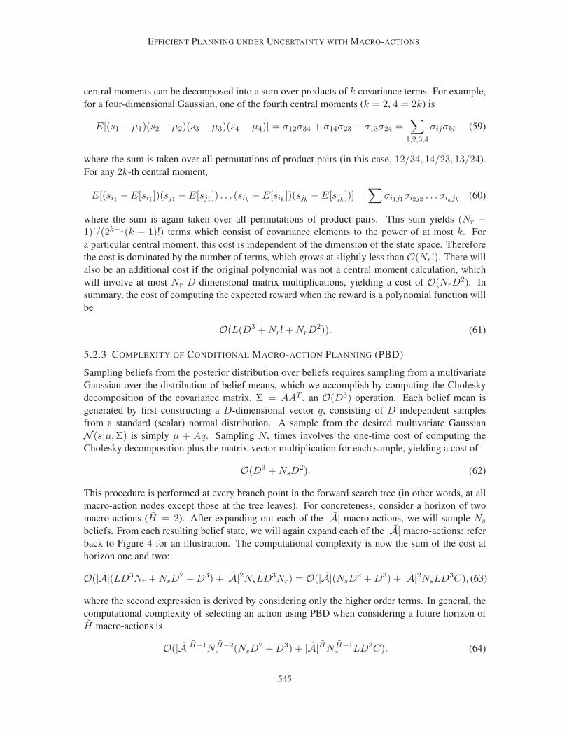
central moments can be decomposed into a sum over products of k covariance terms. For example,
for a four-dimensional Gaussian, one of the fourth central moments (k = 2, 4 = 2k) is
E[(s1 − µ1)(s2 − µ2)(s3 − µ3)(s4 − µ4)] = σ12σ34 + σ14σ23 + σ13σ24 =∑
1,2,3,4
σijσkl (59)
where the sum is taken over all permutations of product pairs (in this case, 12/34, 14/23, 13/24).
For any 2k-th central moment,
E[(si1 − E[si1 ])(sj1 − E[sj1 ]) . . . (sik − E[sik ])(sjk− E[sjk
])] =∑
σi1j1σi2j2 . . . σikjk(60)
where the sum is again taken over all permutations of product pairs. This sum yields (Nr −1)!/(2k−1(k − 1)!) terms which consist of covariance elements to the power of at most k. For
a particular central moment, this cost is independent of the dimension of the state space. Therefore
the cost is dominated by the number of terms, which grows at slightly less than O(Nr!). There will
also be an additional cost if the original polynomial was not a central moment calculation, which
will involve at most Nr D-dimensional matrix multiplications, yielding a cost of O(NrD2). In
summary, the cost of computing the expected reward when the reward is a polynomial function will
be
O(L(D3 + Nr! + NrD2)). (61)
5.2.3 COMPLEXITY OF CONDITIONAL MACRO-ACTION PLANNING (PBD)
Sampling beliefs from the posterior distribution over beliefs requires sampling from a multivariate
Gaussian over the distribution of belief means, which we accomplish by computing the Cholesky
decomposition of the covariance matrix, Σ = AAT , an O(D3) operation. Each belief mean is
generated by first constructing a D-dimensional vector q, consisting of D independent samples
from a standard (scalar) normal distribution. A sample from the desired multivariate Gaussian
N (s|µ,Σ) is simply µ + Aq. Sampling Ns times involves the one-time cost of computing the
Cholesky decomposition plus the matrix-vector multiplication for each sample, yielding a cost of
O(D3 + NsD2). (62)
This procedure is performed at every branch point in the forward search tree (in other words, at all
macro-action nodes except those at the tree leaves). For concreteness, consider a horizon of two
macro-actions (H = 2). After expanding out each of the |A| macro-actions, we will sample Ns
beliefs. From each resulting belief state, we will again expand each of the |A| macro-actions: refer
back to Figure 4 for an illustration. The computational complexity is now the sum of the cost at
horizon one and two:
O(|A|(LD3Nr + NsD2 + D3) + |A|2NsLD3Nr) = O(|A|(NsD
2 + D3) + |A|2NsLD3C), (63)
where the second expression is derived by considering only the higher order terms. In general, the
computational complexity of selecting an action using PBD when considering a future horizon of
H macro-actions is
O(|A|H−1N H−2s (NsD
2 + D3) + |A|HN H−1s LD3C). (64)
545
HE, BRUNSKILL, & ROY
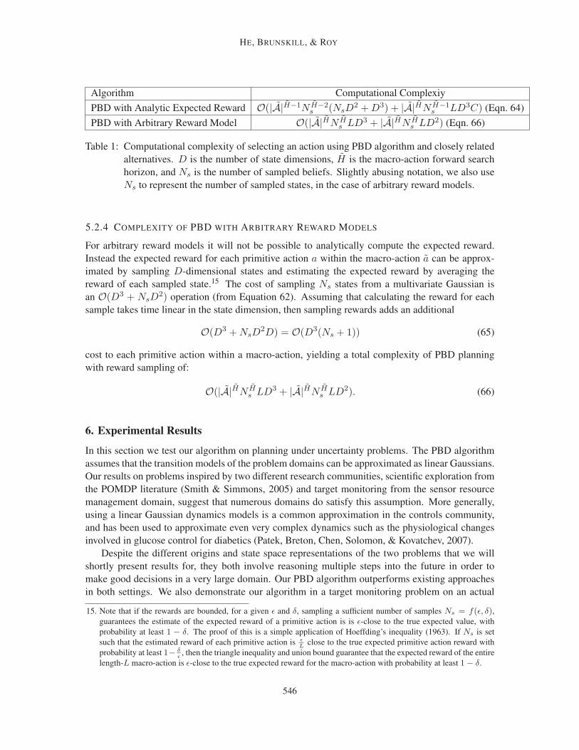
Algorithm Computational Complexiy
PBD with Analytic Expected Reward O(|A|H−1N H−2s (NsD
2 + D3) + |A|HN H−1s LD3C) (Eqn. 64)
PBD with Arbitrary Reward Model O(|A|HN Hs LD3 + |A|HN H
s LD2) (Eqn. 66)
Table 1: Computational complexity of selecting an action using PBD algorithm and closely related
alternatives. D is the number of state dimensions, H is the macro-action forward search
horizon, and Ns is the number of sampled beliefs. Slightly abusing notation, we also use
Ns to represent the number of sampled states, in the case of arbitrary reward models.
5.2.4 COMPLEXITY OF PBD WITH ARBITRARY REWARD MODELS
For arbitrary reward models it will not be possible to analytically compute the expected reward.
Instead the expected reward for each primitive action a within the macro-action a can be approx-
imated by sampling D-dimensional states and estimating the expected reward by averaging the
reward of each sampled state.15 The cost of sampling Ns states from a multivariate Gaussian is
an O(D3 + NsD2) operation (from Equation 62). Assuming that calculating the reward for each
sample takes time linear in the state dimension, then sampling rewards adds an additional
O(D3 + NsD2D) = O(D3(Ns + 1)) (65)
cost to each primitive action within a macro-action, yielding a total complexity of PBD planning
with reward sampling of:
O(|A|HN Hs LD3 + |A|HN H
s LD2). (66)
6. Experimental Results
In this section we test our algorithm on planning under uncertainty problems. The PBD algorithm
assumes that the transition models of the problem domains can be approximated as linear Gaussians.
Our results on problems inspired by two different research communities, scientific exploration from
the POMDP literature (Smith & Simmons, 2005) and target monitoring from the sensor resource
management domain, suggest that numerous domains do satisfy this assumption. More generally,
using a linear Gaussian dynamics models is a common approximation in the controls community,
and has been used to approximate even very complex dynamics such as the physiological changes
involved in glucose control for diabetics (Patek, Breton, Chen, Solomon, & Kovatchev, 2007).
Despite the different origins and state space representations of the two problems that we will
shortly present results for, they both involve reasoning multiple steps into the future in order to
make good decisions in a very large domain. Our PBD algorithm outperforms existing approaches
in both settings. We also demonstrate our algorithm in a target monitoring problem on an actual
15. Note that if the rewards are bounded, for a given ǫ and δ, sampling a sufficient number of samples Ns = f(ǫ, δ),
guarantees the estimate of the expected reward of a primitive action is is ǫ-close to the true expected value, with
probability at least 1 − δ. The proof of this is a simple application of Hoeffding’s inequality (1963). If Ns is set
such that the estimated reward of each primitive action is ǫL
close to the true expected primitive action reward with
probability at least 1− δǫ
, then the triangle inequality and union bound guarantee that the expected reward of the entire
length-L macro-action is ǫ-close to the true expected reward for the macro-action with probability at least 1 − δ.
546

EFFICIENT PLANNING UNDER UNCERTAINTY WITH MACRO-ACTIONS
helicopter platform, underscoring the applicability of our algorithm to real-world domains. In all
results the macro-action search horizon H was chosen empirically given computational constraints,
as is common in forward search approaches. We explicitly explore the performance changes as the
search horizon is varied in Table 3. We did not use a domain-specific estimate of the future node
value of search tree leaf nodes: in some domains it may be easier to specify macro-actions than a
heuristic value function, and a side benefit of PBD is to be able to efficiently search to sufficient
depths such that a heuristic is not required.
6.1 Generic Baselines
In both problems we compare the PBD algorithm to state-of-the-art approaches from the relevant
research community — POMDP planners and sensor resource management algorithms for the sci-
entific exploration and target monitoring problems respectively.
To fully examine the impact of analytically computing the posterior distribution over beliefs,
we also constructed a variety of algorithms that do not currently exist in the literature. These algo-
rithms are given access to the same hand-coded macro-actions as those used by the PBD algorithm.
We first constructed comparison algorithms which use a macro-action forward search but sample
observation trajectories rather than working with a posterior distribution over beliefs. Sampling
observation sequences produces a particle approximation of the resulting distribution over beliefs,
thereby providing a baseline algorithm that does not use an analytic representation of the posterior
belief distribution. These algorithms are referred to as the macro-action discrete (MAD) algorithm
when the underlying state space is discrete, and the macro-action continuous (MAC) algorithm
when the state space is continuous.
We also implemented an offline point-based POMDP solver that was given access to the macro-
actions used by the forward search algorithms.16 Specifically, we modified the state-of-the-art
POMDP planner SARSOP (Kurniawati et al., 2008) algorithm from the Approximate POMDP Plan-
ning (APPL) Toolkit17 and incorporated macro-actions to guide the sampling of belief points that
are used for the point-based value backups. Instead of the SARSOP algorithm using performance
bounds to guide the sampling of the point-based beliefs, the modified SARSOP algorithm uses a
macro-action and a sampled, same-length observation sequence to generate additional point-based
belief samples. This implementation is also a modified version of the MiGS (Kurniawati et al.,
2009) by the same authors. However, due to the offline, point-based nature of this modified algo-
rithm, we were only able to evaluate the algorithm on two of the five problem domains used in this
paper.
Finally, we considered an experimental comparison to an open-loop version of PBD, in which no
conditioning on the received observations is ever performed; however, initial experiments suggested
that this variant performed very poorly in our domains of interest, and so we did not explore it
further.
6.2 Rocksample
The scientific exploration ROCKSAMPLE problem is a benchmark POMDP problem proposed by
Smith and Simmons (2005), and subsequently extended to the FieldVisionRockSample (FVRS)
16. For a formal discussion of the differences between the offline point-based and online forward search POMDP algo-
rithms, we refer the reader to the survey paper by Ross et al. (2008a).
17. Approximate POMDP Planning Toolkit. http://bigbird.comp.nus.edu.sg/pmwiki/farm/appl/
547

HE, BRUNSKILL, & ROY
(a) ISRS(8,5) (b) SARSOP policy (c) PBD policy
Figure 5: Information Search Rocksample (ISRS) problem. (a) Initial (hidden) problem state. An
agent (pink square) explores and samples rocks (circles) in the world. White circles cor-
respond to rocks with positive value, black otherwise. Yellow squares indicate locations
of the rock information beacons. The blue sidebar is the exit region. Red lines indicate
paths taken by an agent executing the (b) SARSOP and (c) PBD policies. We see that
the SARSOP policy only explores rocks and not the beacons; it cannot search far enough
ahead to model the value of the beacons. In contrast, the PBD plan visits the beacons and
then heads directly for the high-value rocks.
problem by Ross and Chaib-draa (2007). Initial experiments in these domains revealed that search-
ing only to a shallow depth was sufficient to obtain good policies. As our interest is in domains
which require long-horizon lookahead, we created a new variant of the ROCKSAMPLE problem
called the Information Search Rocksample (ISRS) problem, shown in Figure 5(a). In ISRS an agent
explores and samples k rocks in a n × n grid world. The positions of the agent (pink square) and
the rocks (circles) are fully observable, but the value of each rock (good or bad) is unknown to the
agent. At every time step, the agent receives a binary observation of the value of each rock. The
accuracy of this observation depends not on the agent’s proximity to the rocks themselves but on
the agent’s proximity to rock information beacons (yellow squares), each of which correspond to
a particular rock (for example, information beacons could be mountain tops that offer a particu-
larly good view of a far off geologic formation). A key characteristic of ISRS that is not present in
ROCKSAMPLE or FVRS is that the rock information beacons are not at the same locations as the
rock themselves. Unlike previous ROCKSAMPLE formulations, information gathering and reward
exploitation require different actions in ISRS.
The agent gets a fixed positive reward for collecting a good rock (white circle), a negative reward
for collecting a bad rock (black circle), and a smaller positive reward for exiting the problem (the
blue sidebar on the right). A discount factor γ = 0.99 encourages the agent to collect rewards
sooner. All other actions have zero rewards.
The observation model is a Bernoulli distribution with the noise of the distribution scaled with
the distance to the beacon, such that:
p(zi,t|si, rt, RBi) =
{
0.5 + (si − 0.5)2−‖rt−RBi‖2
D0 zi,t = 1
0.5− (si − 0.5)2−‖rt−RBi‖2
D0 zi,t = 0(67)
548

EFFICIENT PLANNING UNDER UNCERTAINTY WITH MACRO-ACTIONS
where zi,t is a binary {0 or 1} observation for the value of the rock i at time t,si is the true value {0 or 1} of the rock,
rt is the agent’s position at time t,RBi is the location of the information beacon associated with rock i,D0 is a tuning parameter that controls how quickly the accuracy of the observations
decrease with greater distance between the agent and the beacon.
For example, at an information beacon, the agent, with absolute certainty, receives an observation
that matches the true value of the corresponding rock, whereas when the distance between the agent
and the beacon is infinite, the agent receives an “accurate” observation with 0.5 probability.
All variants of the ROCKSAMPLE problem, including our new ISRS problem, are formulated
with discrete state, action and observation sets. To allow the use of our PBD and MAC algorithms,
we approximate the agent’s belief of each rock’s value as a Gaussian distribution over the [0,1]
state space, and take advantage of the efKF presented in Section 4 to represent the ROCKSAMPLE
problem’s Bernoulli observation model (Equation 67: see Appendix B for details).
Each macro-action is a finite, open-loop sequence of primitive actions. For the ROCKSAMPLE
problem, there are five primitive actions: single steps in the four cardinal directions and the rock
sampling action. Recall that the agent’s position is fully observable and its actions are deterministic.
Using domain knowledge, the macro-actions considered from a particular belief state are macro-
actions that, given the agent’s current position, consist of a sequence of actions that enables the
agent to move to each rock, each information beacon, or to the nearest exit. This results in 2k + 1macro-actions being considered for forward search at every belief node. As the agent operates in
a grid world, there may be multiple action sequences with the same, shortest distance between two
grid squares: the macro-action considered is the one where the agent would move as diagonally as
possible, so as to replicate the agent’s shortest path movement in a continuous map. In addition,
if the agent is currently on a rock (which is fully observable), additional macro-actions where the
agent first collects the rock before executing one of the 2k+1 default macro-actions are considered,
resulting in twice as many macro-actions. The set of macro-actions therefore varies with every
belief node.18 For an ISRS problem with 5 rocks in a 8 × 8 grid world, the average macro-action
length was 4.76, with a minimum and maximum macro-action length of 1 and 12 respectively.
As the ROCKSAMPLE family of problems originates from the POMDP literature, we compared
our macro-action algorithms to existing state-of-the-art POMDP solvers: the fast upper-bound of
QMDP (Littman, Cassandra, & Kaelbling, 1995), the point-based offline value-iteration techniques
HSVI2 (Smith & Simmons, 2005) and SARSOP (Kurniawati et al., 2008), as well as RTBSS (Pa-
quet, Chaib-draa, & Ross, 2006), an online, factored, forward search algorithm. We also evaluated
a modified version of the SARSOP algorithm that was given access to the same macro-actions used
by the forward search macro-action algorithms. Since all approaches, including our own, are ap-
proximations, we also include as an upper bound the value of the fully observable problem.
Table 2 compares the performance of the different algorithms in the ISRS problem. Each algo-
rithm was tested on 10 different initial conditions (which rocks were high valued and which were
low valued), and each scenario was tested 20 times. The HSVI2 and SARSOP algorithms were exe-
cuted offline for a range of durations,19 while the forward search algorithms were allowed to search
18. However, if two belief nodes have the same agent position, their macro-actions will be identical.
19. The offline execution durations for both HSVI2 and SARSOP were chosen empirically. HSVI2 was able to search
for solutions to the ISRS[8,5] problem for 1,000s offline before running out of memory. It was found that the values
computed by SARSOP remained constant after 25,000s.
549
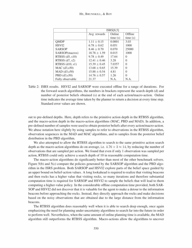
HE, BRUNSKILL, & ROY
ISRS[8,5]
Avg rewards Online
time (s)
Offline
time (s)
QMDP 1.11 ± 0.15 0.0001 3.03
HSVI2 6.78 ± 0.62 0.051 1000
SARSOP 8.46 ± 0.70 0.070 25000
SARSOP(macros) 18.78 ± 1.59 0.015 1000
RTBSS (d5, s10) 9.78 ± 0.49 17.64 0
RTBSS (d7, s2) 12.41 ± 0.46 3.28 0
RTBSS (d10, s1) 15.39 ± 0.45 7.0357 0
MAC (d3,s50) 13.68 ± 0.65 15.39 0
MAD (d3,s50) 15.88 ± 0.54 4.81 0
PBD (d3,s50) 14.76 ± 0.57 1.26 0
Fully observable 21.37 N.A. N.A.
Table 2: ISRS results. HSVI2 and SARSOP were executed offline for a range of durations. For
the forward search algorithms, the numbers in brackets represent the search depth (d) and
number of posterior beliefs obtained (s) at the end of each action/macro-action. Online
time indicates the average time taken by the planner to return a decision at every time step.
Standard error values are shown.
out to pre-defined depths. Here, depth refers to the primitive action depth in the RTBSS algorithm,
and the macro-action depth in the macro-action algorithms (MAC, PBD and MAD). In addition, a
pre-defined number of samples were used to obtain posterior beliefs after every action/macro-action.
We abuse notation here slightly by using samples to refer to observations in the RTBSS algorithm,
observation sequences in the MAD and MAC algorithms, and to samples from the posterior belief
distribution in the PBD algorithm.
We also attempted to allow the RTBSS algorithm to search to the same primitive action search
depth as the macro-action algorithms do on average, i.e. 4.76× 3 ≈ 14, by reducing the number of
observations that are sampled per action. We found that even if only 1 observation was sampled per
action, RTBSS could only achieve a search depth of 10 in reasonable computation time.
The macro-action algorithms do significantly better than most of the other benchmark solvers.
Figure 5(b) and 5(c) compare the policies generated by the SARSOP algorithm and the PBD algo-
rithm in the ISRS problem. Both SARSOP and HSVI2 explore parts of the belief space guided by
an upper bound on belief-action values. A long lookahead is required to realize that visiting beacons
and then rocks has a higher value that visiting rocks, so many iterations and therefore substantial
computation time is required for SARSOP and HSVI2 to sample the beliefs that will lead to them
computing a higher-value policy. In the considerable offline computation time provided, both SAR-
SOP and HSVI2 did not discover that it is valuable for the agent to make a detour to the information
beacons before approaching the rocks. Instead, they directly approach the rocks and make decisions
based on the noisy observations that are obtained due to the large distance from the information
beacons.
The RTBSS algorithm does reasonably well when it is able to search deep enough, once again
emphasizing the need for planning under uncertainty algorithms to search far into the future in order
to perform well. Nevertheless, when the same amount of online planning time is available, the MAD
algorithm still outperforms the RTBSS algorithm. Macro-actions allow the algorithms to uncover
550
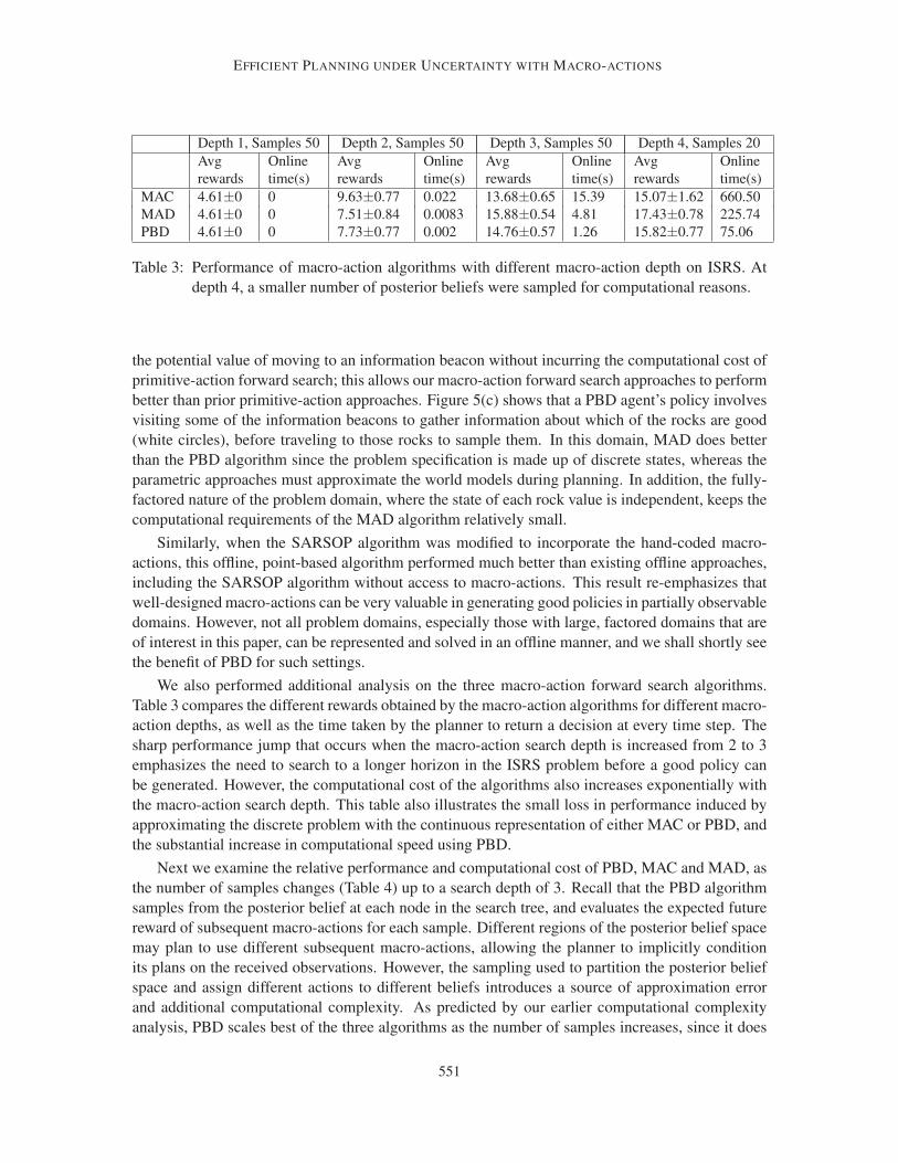
EFFICIENT PLANNING UNDER UNCERTAINTY WITH MACRO-ACTIONS
Depth 1, Samples 50 Depth 2, Samples 50 Depth 3, Samples 50 Depth 4, Samples 20
Avg
rewards
Online
time(s)
Avg
rewards
Online
time(s)
Avg
rewards
Online
time(s)
Avg
rewards
Online
time(s)
MAC 4.61±0 0 9.63±0.77 0.022 13.68±0.65 15.39 15.07±1.62 660.50
MAD 4.61±0 0 7.51±0.84 0.0083 15.88±0.54 4.81 17.43±0.78 225.74
PBD 4.61±0 0 7.73±0.77 0.002 14.76±0.57 1.26 15.82±0.77 75.06
Table 3: Performance of macro-action algorithms with different macro-action depth on ISRS. At
depth 4, a smaller number of posterior beliefs were sampled for computational reasons.
the potential value of moving to an information beacon without incurring the computational cost of
primitive-action forward search; this allows our macro-action forward search approaches to perform
better than prior primitive-action approaches. Figure 5(c) shows that a PBD agent’s policy involves
visiting some of the information beacons to gather information about which of the rocks are good
(white circles), before traveling to those rocks to sample them. In this domain, MAD does better
than the PBD algorithm since the problem specification is made up of discrete states, whereas the
parametric approaches must approximate the world models during planning. In addition, the fully-
factored nature of the problem domain, where the state of each rock value is independent, keeps the
computational requirements of the MAD algorithm relatively small.
Similarly, when the SARSOP algorithm was modified to incorporate the hand-coded macro-
actions, this offline, point-based algorithm performed much better than existing offline approaches,
including the SARSOP algorithm without access to macro-actions. This result re-emphasizes that
well-designed macro-actions can be very valuable in generating good policies in partially observable
domains. However, not all problem domains, especially those with large, factored domains that are
of interest in this paper, can be represented and solved in an offline manner, and we shall shortly see
the benefit of PBD for such settings.
We also performed additional analysis on the three macro-action forward search algorithms.
Table 3 compares the different rewards obtained by the macro-action algorithms for different macro-
action depths, as well as the time taken by the planner to return a decision at every time step. The
sharp performance jump that occurs when the macro-action search depth is increased from 2 to 3
emphasizes the need to search to a longer horizon in the ISRS problem before a good policy can
be generated. However, the computational cost of the algorithms also increases exponentially with
the macro-action search depth. This table also illustrates the small loss in performance induced by
approximating the discrete problem with the continuous representation of either MAC or PBD, and
the substantial increase in computational speed using PBD.
Next we examine the relative performance and computational cost of PBD, MAC and MAD, as
the number of samples changes (Table 4) up to a search depth of 3. Recall that the PBD algorithm
samples from the posterior belief at each node in the search tree, and evaluates the expected future
reward of subsequent macro-actions for each sample. Different regions of the posterior belief space
may plan to use different subsequent macro-actions, allowing the planner to implicitly condition
its plans on the received observations. However, the sampling used to partition the posterior belief
space and assign different actions to different beliefs introduces a source of approximation error
and additional computational complexity. As predicted by our earlier computational complexity
analysis, PBD scales best of the three algorithms as the number of samples increases, since it does
551
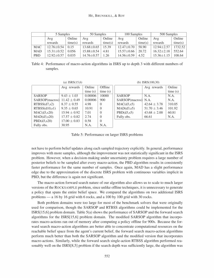
HE, BRUNSKILL, & ROY
5 Samples 50 Samples 100 Samples 500 Samples
Avg
rewards
Online
time(s)
Avg
rewards
Online
time(s)
Avg
rewards
Online
time(s)
Avg
rewards
Online
time(s)
MAC 12.76±0.54 0.15 13.68±0.65 15.39 12.47±0.70 58.90 12.94±2.57 1732.52
MAD 15.31±0.52 0.056 15.88±0.54 4.81 15.57±0.66 20.72 16.32±2.18 552.64
PBD 12.92±0.57 0.035 14.76±0.57 1.26 14.56±0.59 4.52 15.36±1.15 108.64
Table 4: Performance of macro-action algorithms in ISRS up to depth 3 with different numbers of
samples.
(a) ISRS(15,6)
Avg rewards Online
time (s)
Offline
time (s)
SARSOP 9.43 ± 1.03 0.00006 10000
SARSOP(macros) 11.42 ± 0.49 0.00006 900
RTBSS(d7,s2) 8.37 ± 0.55 4.98 0
RTBSS(d10,s1) 9.35 ± 0.65 10.91 0
MAC(d3,s20) 15.94 ± 0.92 7.01 0
MAD(d3,s20) 17.57 ± 0.82 2.74 0
PBD(d3,s20) 17.00 ± 0.83 0.58 0
Fully obs. 30.95 N.A. N.A.
(b) ISRS(100,30)
Avg rewards Online
time (s)
SARSOP N.A. N.A.
SARSOP(macros) N.A. N.A.
MAC(d3,s5) 42.64 ± 3.78 310.05
MAD(d3,s5) 51.70 ± 3.46 101.92
PBD(d3,s5) 43.68 ± 2.00 60.81
Fully obs. 66.61 N.A.
Table 5: Performance on larger ISRS problems
not have to perform belief updates along each sampled trajectory explicitly. In general, performance
improves with more samples, although the improvement was not statistically significant in the ISRS
problem. However, when a decision-making under uncertainty problem requires a large number of
posterior beliefs to be sampled after every macro-action, the PBD algorithm results in consistently
faster performance for the same number of samples. Once again, MAD has a slight performance
edge due to the approximation of the discrete ISRS problem with continuous variables implicit in
PBD, but the difference is again not significant.
The macro-action forward search nature of our algorithm also allows us to scale to much larger
versions of the ROCKSAMPLE problem, since unlike offline techniques, it is unnecessary to generate
a policy that spans the entire belief space. We compared the algorithms on two additional ISRS
problems — a 16 by 16 grid with 6 rocks, and a 100 by 100 grid with 30 rocks.
Both problem domains were too large for most of the benchmark solvers that were originally
used for comparison, though the SARSOP and RTBSS algorithms could be implemented for the
ISRS[15,6] problem domain. Table 5(a) shows the performance of SARSOP and the forward search
algorithms for the ISRS[15,6] problem domain. The modified SARSOP algorithm that incorpo-
rates macro-actions ran out of memory after computing a policy offline for 900s. Because the for-
ward search macro-action algorithms are better able to concentrate computational resources on the
reachable belief space from the agent’s current belief, the forward search macro-action algorithms
perform much better than both the SARSOP algorithm and the modified version that incorporates
macro-actions. Similarly, while the forward search single-action RTBSS algorithm performed rea-
sonably well on the ISRS[8,5] problem if the search depth was sufficiently large, the algorithm was
552
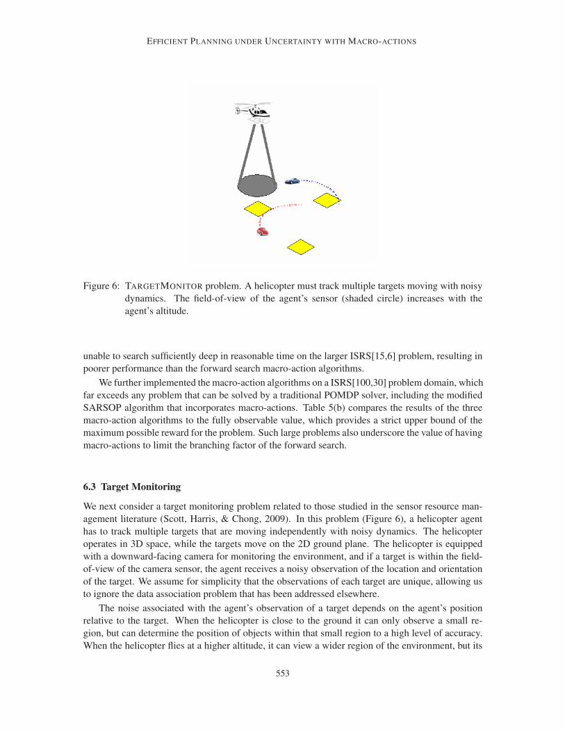
EFFICIENT PLANNING UNDER UNCERTAINTY WITH MACRO-ACTIONS
Figure 6: TARGETMONITOR problem. A helicopter must track multiple targets moving with noisy
dynamics. The field-of-view of the agent’s sensor (shaded circle) increases with the
agent’s altitude.
unable to search sufficiently deep in reasonable time on the larger ISRS[15,6] problem, resulting in
poorer performance than the forward search macro-action algorithms.
We further implemented the macro-action algorithms on a ISRS[100,30] problem domain, which
far exceeds any problem that can be solved by a traditional POMDP solver, including the modified
SARSOP algorithm that incorporates macro-actions. Table 5(b) compares the results of the three
macro-action algorithms to the fully observable value, which provides a strict upper bound of the
maximum possible reward for the problem. Such large problems also underscore the value of having
macro-actions to limit the branching factor of the forward search.
6.3 Target Monitoring
We next consider a target monitoring problem related to those studied in the sensor resource man-
agement literature (Scott, Harris, & Chong, 2009). In this problem (Figure 6), a helicopter agent
has to track multiple targets that are moving independently with noisy dynamics. The helicopter
operates in 3D space, while the targets move on the 2D ground plane. The helicopter is equipped
with a downward-facing camera for monitoring the environment, and if a target is within the field-
of-view of the camera sensor, the agent receives a noisy observation of the location and orientation
of the target. We assume for simplicity that the observations of each target are unique, allowing us
to ignore the data association problem that has been addressed elsewhere.
The noise associated with the agent’s observation of a target depends on the agent’s position
relative to the target. When the helicopter is close to the ground it can only observe a small re-
gion, but can determine the position of objects within that small region to a high level of accuracy.
When the helicopter flies at a higher altitude, it can view a wider region of the environment, but its
553

HE, BRUNSKILL, & ROY
1 Target 2 Targets
Avg rewards Online time (s) Avg rewards Online time (s)
Greedy -21.50 ± 7.65 0.0657 -26.50 ± 5.00 0.19
WT-Single 65.14 ± 8.64 0.00075 -27.03 ± 8.06 0.00068
WT-Macro 64.64 ± 8.28 0.00076 -19.05 ± 7.64 0.00042
NBO -5.80 ± 7.92 0.051 -10.78 ± 6.95 0.21
MAC(d2,s10) 41.73 ± 6.96 4.73 46.67 ± 18.91 22.13
MAD(d2,s3) 1.27 ± 5.23 1.66 0.97 ± 5.82 8.46
PBD(d2,s10) 36.21 ± 6.52 0.89 68.00 ± 16.65 4.33
3 Targets 8 Targets
Greedy -18.00 ± 7.15 0.46 -95.00 ± 23.37 2.01
WT-Single -23.52 ± 10.89 0.00080 -71.17 ± 14.53 0.00063
WT-Macro -10.53 ± 17.12 0.00037 -52.98 ± 21.74 0.00025
NBO -8.27 ± 8.84 0.63 -5.98 ± 18.00 5.78
MAC(d2,s10) 37.89 ± 12.49 70.91 83.86 ± 25.65 711.67
MAD(d2,s3) -1.86 ± 5.19 26.96 27.36 ± 14.74 432.13
PBD(d2,s10) 55.78 ± 13.84 13.02 120.80 ± 25.77 132.50
Table 6: TARGETMONITOR Results. Run for 200 time steps.
measurements will be less precise. Similarly, the closer the helicopter is to a particular target, the
more accurate the helicopter’s observation of that target is expected to be. Reflecting this intuition,
we use a Gaussian observation model where the noise covariance is a function of the position of
the helicopter and target: details of this sensor model are provided in Appendix C. One desirable
attribute of our sensor model is that if the helicopter is very uncertain about a target’s location, even
if the helicopter is close to the target’s mean location, a single observation is unlikely to localize the
target. If the target location is very uncertain, there is a low probability that the target is within the
helicopter’s field of view.
The agent’s pose is fully observable, though the actions that it takes are subject to a small amount
of additive Gaussian noise. As a result, unlike the ROCKSAMPLE domains, the open-loop nature of
macro-actions means that the planner cannot perfectly predict the vehicles’ pose at the end of the
macro-action. Each target’s motion is determined by its translational and rotational velocities. The
model provides the agent with a prior over these velocities, but at every time step, the target’s true
velocities are additive functions of these fixed input controls and Gaussian noise. In the parametric
formulation, the agent maintains a Gaussian belief over each target’s state, and in order to compare
MAD, we discretize the continuous state spaces of the agent’s and targets’ positions, and maintain
a probability distribution over each discrete target state. Due to computational memory constraints,
for a 100m by 100m by 20m target monitoring problem in the x, y and z directions, we were limited
to a discretization with 10m resolution in the x, y directions, 5m in the z direction, and 45◦ angular
resolution.
We focus on a particular decision-theoretic version of the sensor resource management problem,
where at each time step the agent must decide if each of the targets is inside an area of interest.
These areas of interest are indicated by the yellow squares in Figure 6. The agent receives a positive
reward if it successfully reports that a target is in an interest region, a negative reward if it wrongly
decides that the target is in the region, and no reward if it decides that the target is not in the region,
regardless of the target’s actual state. Small costs are incurred for the agent’s motion. We call this
the TARGETMONITOR problem.
554
EFFICIENT PLANNING UNDER UNCERTAINTY WITH MACRO-ACTIONS
Given the current location of the agent, macro-actions were generated by computing the se-
quence of actions that will enable the agent to move to a particular altitude over the means of each
target belief. For a particular desired destination, a macro-action is constructed by first comput-
ing the shortest path between the agent’s current and desired location, and then dividing this path
into primitive actions based on the maximum length of each primitive action. We also included a
hovering macro-action that consists of hovering at the agent’s current location for four time steps.
Note that the agent’s current location is fully-observable, and for the purpose of generating macro-
actions, we assume that the primitive actions are noise-free. Hence, for each primitive action, the
helicopter is assumed to move by the mean expected change. Similar to the ROCKSAMPLE problem,
although the macro-actions are generated according to a policy that relies on domain knowledge, the
macro-actions themselves are evaluated in the forward-search algorithms as open-loop sequences
of primitive actions. We compare the forward search macro-action algorithms to a range of intu-
itive strategies and prior approaches. The first algorithm is the greedy strategy, which returns the
primitive action that results in the largest expected reward in the next step. The next two approaches
are the Worst Target (WT) policies, which are hand-coded policies of traveling to the target that
has the largest uncertainty of all the targets being tracked. The intuition is that the agent’s goal in
general is to localize the targets in the environment. The two algorithms differ based on whether
the agent chooses a new target to travel to after each time step (WT-single), or re-plans only after
it has reached the target it had initially chosen (WT-macro). Finally, we compared our algorithm to
the nominal belief optimization (NBO) algorithm proposed by Scott, Harris and Chong (2009). The
NBO algorithm also assumes a Kalman filter model for the target monitoring problem, but rather
than considering the entire distribution of posterior beliefs, only the most likely posterior belief af-
ter an action is considered. In this algorithm, the most likely posterior belief for a Gaussian belief
update is given by the posterior mean without incorporating any observations, and the covariance
given by linearizing about the most likely mean at each step. Although the original algorithm uses
an optimization approach to search for action sequences, here we modify the NBO algorithm by
adopting a forward search approach, evaluating each macro-action based on the most likely poste-
rior belief.20
Table 6 presents results for the TARGETMONITOR problem, comparing the algorithms in sce-
narios with different number of targets. These results demonstrate that the PBD algorithm, with
its closed form representation of the distribution of posterior beliefs after an action, finds a signifi-
cantly better policy than alternate approaches. Figure 7 demonstrates a typical policy executed by
the PBD algorithm. The agent begins in the middle of the grid world, and approaches a target at a
high altitude (Figure 7(b)), maximizing the likelihood of localizing that target. If none of the targets
seem to be approaching a region of interest, the agent hovers in the same position to conserve energy
(Figure 7(c)). When one of the targets may potentially be entering a region of interest, the agent
focuses on that target, tracking it carefully to ensure that it knows when the target is exactly in the
region of interest (Figure 7(d),(e)). The agent subsequently travels to a high altitude and repeats the
process of localizing another target with potential rewards (Figure 7(f)).
Considering the entire distribution of posterior beliefs, rather than just the maximum likelihood
posterior belief, is valuable because the agent is able to reason that there is a possibility that the
20. As noted by the authors, the NBO algorithm focuses on a new method for approximating the Q-value, rather than on
the optimization techniques. While they adopt a generic search approach for performing the optimization, the authors
also point to forward-search POMDP algorithms as good search techniques in which their Q-value approximations
could be incorporated. Our use of forward search with the NBO Q-value approximation does not affect the results.
555

HE, BRUNSKILL, & ROY
(a) (b) (c)
(d) (e) (f)
Figure 7: Snapshots of the PBD policy being executed. The black circle indicates the field-of-view
of the agent’s sensor, which is directly proportionate to the agent’s height. The size of
the error ellipses indicate the agent’s uncertainty associated with each target at each time
step. The agent alternates between flying at a high altitude to maximize the likelihood of
observing targets (b),(f) and focusing on a single target that is near/has entered an area of
interest (e).
target could be within a region of interest. In contrast, the NBO approach only considers the most
likely posterior belief, and will seek to localize the target only if the mean of its belief appears to
be heading into a region of interest. While the consideration of the entire distribution of posterior
beliefs necessarily incurs greater computational cost, we demonstrate in Section 6.4 that we are able
to track two targets in real-time using an implementation of the PBD algorithm that has not been
optimized for speed.
Table 6 also shows that because the PBD algorithm directly computes the distribution of poste-
rior beliefs after a macro-action, the computational cost of the PBD algorithm is significantly lower
than the MAC algorithm. The MAC algorithm suffers a greater computational cost as it generates
the set of posterior beliefs after a macro-action by sampling observation sequences and explicitly
performing belief updating along each sample trajectory. In addition, because the TARGETMON-
ITOR problem has a state space that is fundamentally continuous, the resolution of the state space
556

EFFICIENT PLANNING UNDER UNCERTAINTY WITH MACRO-ACTIONS
(a) Our Quadrotor helicopter (b) Multiple cars being tracked. (c) Helicopter tracking car through an
area of interest
Figure 8: TARGETMONITOR demonstration with helicopter. The helicopter has to simultaneously
track two cars and report whenever either car enters an area of interest.
discretization that was achievable given computational memory constraints was still unable to cap-
ture the inherent characteristics of the target monitoring problem, resulting in the poor performance
of MAD in the TARGETMONITOR problem.
In the single-target case, we also observed the result that the PBD algorithm does worse than the
hand-coded policy of the agent traveling to the target with the largest uncertainty (WT-single). When
the problem only involves a single target, such a policy equates to having the agent hover over the
sole target at every step, which is the optimal policy in the single target case. In contrast, we observe
that the MAC and PBD algorithms return policies that result in the agent periodically leaving the
target to fly to a higher altitude, resulting in greater noise in the observations and corresponding loss
of rewards on average. By restricting the MAC and PBD algorithms to planning with macro-actions,
we restrict the set of plans the agent can consider in order to search deeper, rather than a shorter
conditional plan that is conditioned on the observations after each primitive action. Even though
the agent re-plans after every time step, without this conditional plan, an agent executing the MAC
or PBD algorithms will execute the “safe” policy and fly to a higher altitude, which maximizes the
likelihood of keeping the target well-localized when it is unable to condition its actions based on
subsequent observations. This example highlights the trade-off we make by considering a smaller
class of policies (those that can be expressed as chains of macro-actions) compared to the full
policy set. While in simple problems, such as a single-target TARGETMONITOR problem, the policy
restriction can clearly be a limitation, our macro-action algorithms perform significantly better than
the other benchmark approaches when there are multiple targets, in scenarios that are arguably more
complicated and require more sophisticated planning algorithms.
6.4 Real-world Helicopter Experiments
Finally, as a proof of concept, we demonstrate the PBD algorithm on a live instantiation of the
TARGETMONITOR problem. A motivating application for this monitoring problem is our involve-
ment (He et al., 2010a) in the 1st US-Asian Demonstration and Assessment of Micro Aerial Vehicle
(MAV) and Unmanned Ground Vehicle (UGV) Technology (MAV’08 competition). The mission
was a hostage rescue scenario, where an aerial vehicle had to guide ground units to a hostage build-
ing while avoiding an enemy guard vehicle. Our aerial vehicle therefore had to plan paths in order
557

HE, BRUNSKILL, & ROY
Figure 9: The helicopter (blue/red cross) uses an onboard laser scanner to localize itself. A down-
ward pointing camera is used to observe the ground targets. In this figure, the camera
image from the onboard camera is projected onto the ground plane.
to be able to monitor the different ground objects and report whenever any of them arrived at an
area of interest.
We demonstrate this scenario on an actual helicopter platform monitoring multiple ground vehi-
cles in an indoor environment (Figure 8b). In previous work (He, Prentice, & Roy, 2008; Bachrach,
He, & Roy, 2009), we developed a quadrotor helicopter (Figure 8a) that is capable of autonomous
flight in unstructured and unknown indoor environments. The helicopter uses a laser rangefinder to
localize itself in the environment.
We mounted a downward-facing camera to make observations of the target. Since target detec-
tion is not the focus of this paper, each of the ground vehicles had a known, distinctive color, to
be detected and distinguished easily with a simple blob detection algorithm. Given the helicopter’s
position in the world and the image coordinates of the detected object, we were able to recover an
estimate of the position and orientation of a target observation in global coordinates. The helicopter
only received an observation of the target when the target was within the camera’s field-of-view,
and although the helicopter platform hovered relatively stably, slight oscillations persisted, which
resulted in noisier observations when the helicopter was flying at higher altitudes. Hence, the he-
licopter had to choose actions that balanced between obtaining more accurate observations at low
altitudes and a larger field-of-view by flying high.
Two ground vehicles were driven autonomously in the environment with open-loop control,
and the helicopter had to plan actions that would accurately localize both targets. To replicate
the TARGETMONITOR problem, we marked out three areas of interest where the helicopter had to
558

EFFICIENT PLANNING UNDER UNCERTAINTY WITH MACRO-ACTIONS
(a) (b) (c) (d)
Figure 10: Bird’s eye-view snapshots of the helicopter’s trajectory (red), based on policy generated
by the PBD algorithm. The helicopter (blue/red cross) alternates between observing the
white (b,d) and blue (c) cars in order to accurately report when either car is in an area of
interest. The area of the field-of-view of the agent’s camera sensor varies directly with
the height that the agent is flying at.
# Target entry detections # True target entries Flight time (s) Dist. traveled (m)
WT-Single 1 7 484.15 243.36
NBO 1 4 435.25 247.01
PBD 4 6 474.64 282.51
Table 7: Performance of algorithms on real-world helicopter experiment. Ground truth was found
using an overhead video camera.
predict at every time step if the targets were within those areas (Figure 8c). We applied the PBD
algorithm to plan paths for the helicopter that maximized the likelihood that it could accurately
report whenever a target is in an area of interest. However, rather than sending open-loop control
actions to the helicopter, as we did in the simulation experiments, for safety reasons we closed the
loop around the position of the helicopter, sending desired waypoints that we wanted the helicopter
to navigate to. The helicopter’s true state in the world was actually partially observable, and the
helicopter had to rely on an onboard laser scanner to localize its position in the environment.
Figure 9 shows a 3D view of the helicopter as it monitors and reports on the locations of the
ground targets. As the helicopter flew around the environment, it obtained observations of the target,
which were then used to update the agent’s belief of the targets. Figure 10 provides snapshots of
the helicopter executing a plan that is computed online by the PBD algorithm. The helicopter ex-
hibited similar behaviors to those that were observed in the simulation experiments. The helicopter
alternated between the two targets in the environment to report when either target was in an area of
interest. When the agent had a large uncertainty over a particular target’s location, it would also fly
to a higher altitude in order to increase its sensor field-of-view, thereby maximizing the likelihood
that it will be able to re-localize the targets. A video of the complete system in action is available
at: http://groups.csail.mit.edu/rrg/index.php?n=Main.Videos.
559

HE, BRUNSKILL, & ROY
As a coarse measure of achieved reward, we evaluated how well the helicopter running PBD
did at monitoring when a target entered an area of interest, and compared it to the WT-Single and
NBO algorithms. The ground truth of the number of times the targets actually entered the areas of
interests in each trial was found by using a video camera mounted overhead above the environment.
Table 7 indicates that the PBD algorithm did a much better job of monitoring the targets’ positions
than both the WT-Single and NBO algorithms. In particular, we observed that both the WT-Single
and NBO algorithms seldom took advantage of the ability to increase the agent’s sensor field-of-
view by having the agent fly to a higher altitude. An agent applying these two algorithms therefore
had a higher probability of losing track of the targets completely.
7. Related Work
Decision-making under uncertainty when the states are partially observable is most commonly dis-
cussed under the Partially Observable Markov Decision Process (POMDP) framework, though this
problem has also been analyzed in other research domains under similar assumptions. While it is
beyond the scope of this paper to provide a comprehensive survey of POMDP techniques, point-
based methods such as HSVI2 (Smith & Simmons, 2005) and SARSOP (Kurniawati et al., 2008) are
often considered state-of-the-art offline methods, leveraging the piece-wise and convex aspects of
the value function to perform value updates at selected beliefs. These approaches assume a discrete-
state representation, but offline approaches that use parametric representations have been proposed
for continuous-valued state spaces (Brooks, Makarenko, Williams, & Durrant-Whyte, 2006; Brun-
skill, Kaelbling, Lozano-Perez, & Roy, 2008; Porta et al., 2006). Hoey and Poupart (2005) have
also addressed continuous observation spaces by finding lossless partitions of the observation space.
Recent work by Bonet and Geffner (2009) suggests that alternate point-based approaches that use
tabular representations of the value function may also be competitive with prior point-based ap-
proaches which used α-vector representations, and this alternate representation may be useful for
continuous domains. The ideas in this paper are more closely related to the body of online, forward
search POMDP techniques that only compute an action for the current belief, which were recently
surveyed by Ross et al. (2008a).
Macro-actions have been considered in depth within the fully observable Markov decision pro-
cess community, and are typically known as “options” (Sutton et al., 1999), or posed as part of
a semi-Markov decision process (Mahadevan, Marchalleck, Das, & Gosavi, 1997). These prior
formalisms for temporally-extended actions include closed-loop policies that persist until a termi-
nation state is achieved. It would be interesting to explore in the future how these richer notions of
macro-actions could be incorporated into our approach.
Several offline POMDP approaches use macro-actions such as those of Pineau, Gordon, and
Thrun (2003b), Hansen and Zhou (2003), Charlin, Poupart, and Shioda (2007), Foka and Tra-
hanias (2007), Theocharous and Kaelbling (2003) and Kurniawati et al. (2009). Pineau et al.’s
PolCA+ (2003b) algorithm uses a hierarchical approach to solving discrete-state POMDPs. Sim-
ilarly, Hansen and Zhou (2003) propose hierarchical controllers that exploit a user-specified hier-
archy for planning, while Charlin et al. (2007) provide a method for automatically discovering a
problem hierarchy. Yu, Chuang, Gerkey, Gordon and Ng (2005) provide an optimal algorithm for
planning if no observations were available. Foka and Trahanias’s (2007) solution involves building
a hierarchy of nested representations and solutions. Their focus is on discrete-state problems, par-
ticularly navigation applications. Theocharous and Kaelbling’s (2003) discrete-state reinforcement
learning approach samples observation trajectories and solves for the expected reward of a discrete
560

EFFICIENT PLANNING UNDER UNCERTAINTY WITH MACRO-ACTIONS
set of belief points using function approximation. Kurniawati et al. (2009) recently used macro-
actions to guide the sampling of belief points for use in an offline point-based POMDP solver.
However, these prior macro-action POMDP approaches compute a value function off-line, are
not aimed at scaling to very large domains, and will struggle in the environments considered in this
paper. An exception to this is the work by Hsiao and colleagues (2008, 2010) who used a form
of macro-actions for those robot manipulation tasks that involve a large state space. The focus of
their work is on robust manipulation under uncertainty, and their work only considers a very short
horizon of action trajectories. Except for the work by Kurniawati et al. (2009), all these macro-
action POMDP approaches, like our PBD algorithm, assume the macro-actions are provided by a
domain expert.
In the sensor resource management domain, planning under uncertainty techniques are used in
the context of planning sensor placements to track single or multiple targets. Existing algorithms
often adopt a myopic, or greedy strategy when it comes to planning (Krause & Guestrin, 2007),
but notable exceptions include the work by Scott et al. (2009) and Kreucher, Hero III, Kastella,
and Chang (2004). Kreucher et al. describe a multi-target tracking problem, where non-myopic
sensor management is necessary for multi-target tracking. The authors use a particle filter approach
to represent the agent’s belief of the target’s location, and seek to find paths that will result in the
greatest KL divergence in density before and after the measurement. To look ahead more than
one action, this algorithm uses Monte Carlo sampling to generate possible observation outcomes.
They also provide an information-directed path searching scheme to reduce the complexity of the
Monte Carlo sampling, as well as value heuristics that will help direct the search. It is possible
that some of their insights could be used in combination with our macro-action formulation to
strengthen both approaches. In the experimental section we compared our approach to the work by
Scott et al. (2009), who directly formulated target tracking as a POMDP, and proposed the Nominal
Belief Optimization (NBO) algorithm that computes the most likely belief after an action for deeper
forward search. In contrast, our algorithm explicitly computes the entire set of possible posterior
beliefs after a macro-action. Recently two groups (Erez & Smart, 2010; Platt, Tedrake, Lozano-
Perez, & Kaelbling, 2010) have independently proposed an approach that lies in the middle of this
spectrum: beliefs are updated by assuming that the most likely observation is received, but the
variance is increased. In contrast, our approach represents that each resulting belief may be fairly
peaked, but the mean of the beliefs may be spread out. This more complete representation may be
advantageous if there are sharp changes in the reward function.
As stated in the introduction, the finite-horizon forward search, act, and re-plan strategy PBD
follows can be seen as an instance of the Model Predictive Control/Receding Horizon Control
(MPC/ RHC) framework from the controls community. Examples of MPC and RHC include the
work by Kuwata and How (2004), Bellingham, Richards, and How (2002), and Richards, Kuwata,
and How (2003). A special case of RHC control is Certainty Equivalence Control, or CEC (see Bert-
sekas, 2007 for an overview). In fully observable systems, CEC first assumes all stochastic opera-
tions (such as transitions) take on their expected value, and then solves a finite-horizon deterministic
control problem. CEC may be applied in partially observable environments by first sampling an
initial state from the belief state. Though CEC can be very efficient in large domains, a key limi-
tation of its use in partially observable environments is that a CEC-style controller will never take
information-gathering actions. Returning to the generic class of MPC approaches, to our knowledge
no prior model predictive controllers have used macro-actions nor developed the notion of a pos-
561

HE, BRUNSKILL, & ROY
terior distribution of beliefs, which enables our PBD approach to scale to large uncertain domains
where a multi-step lookahead is required.
8. Conclusion
In this paper we have presented the Posterior Belief Distribution algorithm. PBD is a forward-
search algorithm for large (consisting of many variables, each of which can take on many values)
partially observable domains. PBD analytically and efficiently computes the resulting distribution
of posterior belief states possible after a sequence of actions. This allows the computational cost
of evaluating the reward associated with a macro-action to be tractable, which we leverage to en-
able longer horizon lookahead search during online planning. We have presented theoretical and
experimental results evaluating the performance and computational cost of our macro-action algo-
rithms. Our algorithms were applied to problem domains that span multiple research communities,
and consistently performed better than prior approaches in large domains which require multi-step
lookahead for good performance. Finally, we demonstrated our algorithm on a real robotic he-
licopter, underscoring the applicability of our algorithm for planning in real-world, long-horizon,
partially observable domains.
9. Acknowledgments
Ruijie He, E. Brunskill and N. Roy were supported by the National Science Foundation (NSF)
Division of Information and Intelligent Systems (IIS) under Grant #0546467 and by the Office
of Naval Research under the “Decentralized Reasoning in Reduced Information Spaces” project,
Contract # N00014-09-1-1052.
We wish to thank Finale Doshi-Velez, Alborz Geramifard, Josh Joseph, Brandon Luders, Javier
Velez, and Matthew Walter for valuable discussions and feedback. Daniel Gurdan, Jan Stumpf
and Markus Achtelik provided the quadrotor helicopter and the support of Ascending Technolo-
gies. Abraham Bachrach, Anton De Winter, Garrett Hemann, Albert Huang, and Samuel Prentice
assisted with the development of the software and hardware for the helicopter demonstration. We
also appreciate early POMDP forward search discussions with Leslie Pack Kaelbling and Tomas
Lozano-Perez.
Appendix A: Exponential Family Kalman Filter
Building on statistical economics research for time-series analysis of non-Gaussian observations (Durbin
& Koopman, 2000), we present the Kalman filter equivalent for systems with linear-Gaussian state-
transitions and observation models that belong to the exponential family of distributions.
The state-transition and observation models can be represented as follows:
st = Atst−1 + Btat + εt, st−1 ∼ N(µt−1, Σt−1), εt ∼ N(0, Pt) (68)
p(zt|θt) = exp(zTt θt − βt(θt) + κt(zt)), θt = W (st). (69)
For the state-transition model, st is the system’s hidden state, at is the control actions, At and Bt
are the linear transition matrices, and ǫt is the state-transition Gaussian noise with covariance Pt.
The observation model belongs to the exponential family of distributions. θt and βt(θt) are
the canonical parameter and normalization factor of the distribution, and W (.) maps the states to
canonical parameter values. W (.) depends on the particular member of the exponential family. For
562

EFFICIENT PLANNING UNDER UNCERTAINTY WITH MACRO-ACTIONS
ease of notation, we let
υt(zt|θt) = − log p(zt|θt) = −zTt θt + βt(θt) + κt(zt). (70)
Following the traditional Kalman filter, the process update can be written as
µt = Atµt−1 + Btat, Σt = AtΣt−1ATt + Pt, (71)
where µt and Σt are the mean and covariances of the posterior belief after the process update but
before the measurement udpate. For the measurement update, we seek to find the conditional mode
µt = arg maxst
p(st|zt) (72)
= arg maxst
p(zt|st)b(st) (Bayes rule) (73)
= arg maxst
p(zt|θt)b(st) (74)
= arg maxst
exp(−Jt), where Jt = − log p(zt|θt) +1
2(st − µt)
T Σ−1t (st − µt) (75)
⇒ 0 =∂Jt
∂st
∣
∣
∣
st=µt
=∂υt(zt, θt)
∂θt
∂θt
∂st+ Σ
−1t (µt − µt). (76)
Taking the derivative of θt = W (st) about the prior mean µt, we let
Yt =∂W (st)
∂st
∣
∣
∣
∣
st=µt
. (77)
Similarly, performing a Taylor expansion on∂υt(zt|θt)
∂θtabout θt = W (µt),
∂υt(zt|θt)
∂θt=
∂υt(zt|θt)
∂θt
∣
∣
∣
∣
θt=θt
+∂2υt(zt|θt)
∂θt∂θTt
∣
∣
∣
∣
θt=θt
(θt − θt) (78)
∂υt(zt|θt)
∂θt=υt + υt(θt − θt) (79)
where υt =∂
∂θt(−zT
t θt + βt(θt)− κt(zt))
∣
∣
∣
∣
θt=θt
, (Eqn. 70) (80)
=∂βt(θt)
∂θt
∣
∣
∣
∣
θt=θt
−zt (81)
υt =βt − zt (82)
and υt =∂2βt(zt|θt)
∂θt∂θTt
∣
∣
∣
∣
θt=θt
(θt − θt). (83)
υt =βt (84)
Plugging Equations 82 and 84 into Equation 79, and then into Equation 76,
Y Tt (βt − zt + βt(θt − θt)) =− Σ
−1t (µt − µt) (85)
Y Tt βt(β
−1t (βt − zt)− θt + θt) =− Σ
−1t (µt − µt) (86)
Y Tt βt((θt − β−1
t (βt − zt))− θt) =Σ−1t (µt − µt) (87)
Y Tt βt(zt −W (st)) =Σ
−1t (µt − µt), (88)
563

HE, BRUNSKILL, & ROY
where zt = (θt − β−1t (βt − zt)) is the projection of the observation onto the parameter space of
the exponential family distribution, and is independent of st. In Equation 88 we substituted θt using
Equation 69.
Mean Update
Using Equation 88 and substituting µt for st,
Σ−1t (µt − µt) = Y T
t βt(zt −W (µt)) (89)
= Y Tt βt(zt −W (µt)) + W (µt)−W (µt) (90)
= Y Tt βt(zt −W (µt))− Y T
t βt(W (µt)−W (µt)). (91)
Linearizing W (st) about µt,
W (st) = W (µt) + W ′(st)st=µt(st − µt) (92)
= W (µt) + Yt (µt − µt) (93)
⇒ Σ−1t (µt − µt) = Y T
t βt(zt −W (µt))− Y Tt βtYt (µt − µt) (94)
Y Tt βt(zt −W (µt)) = (Σ
−1t + Y T
t βtYt )(µt − µt) (95)
= Σ−1t (µt − µt) (96)
⇒ µt − µt = ΣtYTt βt(zt −W (µt)), (97)
where ΣtYTt βt = Kt is the Kalman gain for non-Gaussian exponential family distributions. Via a
standard transformation, the Kalman gain can be written in terms of covariances other than Σt,
Kt = ΣtYTt (YtΣtY
Tt + β−1
t )−1 (98)
and µt = µt + Kt(zt −W (µt)). (99)
Covariance Update
Given a Gaussian posterior belief, ∂2J∂s2
t
is the inverse of the covariance of the agent’s belief
Σ−1t =
∂2J
∂s2t
(100)
=∂
∂x(Σ
−1t (st − µt)− Y T
t βt(zt −W (st))) (101)
= Σ−1t + Y T
t βtYt (102)
⇒ Σt = (Σ−1t + Y T
t βtYt)−1. (103)
Appendix B. Rock Sample Observation Model
In the Rocksample problem, the Bernoulli observation function can be written as follows. Recall
that rt is the agent’s position at time t, RBi is the location of the information beacon associated
with rock i, zi,t is a binary observation of the value of rock i at time t, and si,t is the true value of
564
EFFICIENT PLANNING UNDER UNCERTAINTY WITH MACRO-ACTIONS
rock i at time t. Then if we let di,t =‖ rt −RBi ‖2, then
p(zi,t|RVi,t = si,t, rt, RBi) (104)
= (0.5 + (si,t − 0.5)2−di,t/D0)zi,t(0.5− (si,t − 0.5)2−di,t/D0)1−zi,t (105)
= exp(zi,t ln0.5 + (si,t − 0.5)2−di,t/D0
0.5− (si,t − 0.5)2−di,t/D0
+ ln(0.5− (si,t − 0.5)2−di,t/D0)) (106)
= exp(zi,tθt − βt(θt)). (107)
We therefore have the parameters of the exponential family observation model
θi,t = W (si,t, rt, RBi) (108)
= ln0.5 + (si,t − 0.5)2−di,t/D0
0.5− (si,t − 0.5)2−di,t/D0
(109)
βi,t = − ln(0.5− (si,t − 0.5)2−di,t/D0) (110)
= ln(exp(θi,t) + 1). (111)
We can then derive the derivatives Yi,t and βi,t
Yt =∂W (si,t, rt, RBi)
∂si,t
∣
∣
∣
∣
si,t=mi,t
(112)
=∂
∂si,tln
0.5 + (si,t − 0.5)2−di,t/D0
0.5− (si,t − 0.5)2−di,t/D0
∣
∣
∣
∣
si,t=mi,t
(113)
=2−di,t/D0
0.5 + (mi,t − 0.5)2−di,t/D0
· 1
0.5− (mi,t − 0.5)2−di,t/D0
(114)
where si,t is the mean of the belief used for linearization. Since
⇒ βi,t = ln(exp(θi,t) + 1), (115)
then
βi,t =∂2bi,t
∂θ2i,t
∣
∣
∣
∣
θi,t=θi,t
(116)
=exp(θi,t)
exp(θi,t) + 1− exp(2θi,t)
(exp(θi,t) + 1)2. (117)
Appendix C. Target Tracking Observation Model
We adopt an observation model for target tracking where the target observation obtained has Gaus-
sian noise and the noise covariance Σzi is a function of the position of the helicopter and target
i:
zxi
zyi
zθi
= f
xi
yi
θi
+N (0, Σzi)
Σzi = g(xi, yi, xa, ya, ha),
565
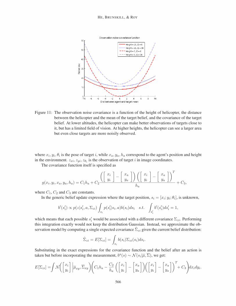
HE, BRUNSKILL, & ROY
Figure 11: The observation noise covariance is a function of the height of helicopter, the distance
between the helicopter and the mean of the target belief, and the covariance of the target
belief. At lower altitudes, the helicopter can make better observations of targets close to
it, but has a limited field of vision. At higher heights, the helicopter can see a larger area
but even close targets are more noisily observed.
where xi, yi, θi is the pose of target i, while xa, ya, ha correspond to the agent’s position and height
in the environment. zxi, zyi, zθiis the observation of target i in image coordinates.
The covariance function itself is specified as
g(xi, yi, xa, ya, ha) = C1ha + C2
([
xi
yi
]
−[
xa
ya
])([
xi
yi
]
−[
xa
ya
])T
ha+ C3,
where C1, C2 and C3 are constants.
In the generic belief update expression where the target position, si = [xi; yi; θi], is unknown,
b′(s′i) ∝ p(z|s′i, a,Σzi)
∫
si
p(s′i|si, a)b(si)dsi s.t.
∫
s′i
b′(s′i)ds′i = 1,
which means that each possible s′i would be associated with a different covariance Σzi. Performing
this integration exactly would not keep the distribution Gaussian. Instead, we approximate the ob-
servation model by computing a single expected covariance Σzi given the current belief distribution:
Σzi = E[Σzi] =
∫
si
b(si)Σzi(si)dsi.
Substituting in the exact expressions for the covariance function and the belief after an action is
taken but before incorporating the measurement, ba(s) ∼ N (si|µ,Σ), we get:
E[Σzi] =
∫
N([
xi
yi
] ∣
∣
∣
∣
µxy, Σxy
)
(
C1ha −C2
ha
([
xi
yi
]
−[
xa
ya
])([
xi
yi
]
−[
xa
ya
])T
+ C3
)
dxidyi.
566
EFFICIENT PLANNING UNDER UNCERTAINTY WITH MACRO-ACTIONS
and by adding and subtracting µxy from the second term, reduces to
E[Σzi] = C1ha +C2
ha
(
µxy −[
xa
ya
])(
µxy −[
xa
ya
])T
+C2
haΣxy
where µxy, Σxy refer to the translational components of the agent’s belief.
In contrast to simpler observation models, our observation model has the desirable characteristic
that if a target’s location is very uncertain, namely its covariance Σxy is very large, then even if the
target’s mean location is close to the helicopter’s mean location, the expected benefit of receiving
an observation (in terms of reducing the target’s uncertainty) is still small. This property comes out
automatically from the above derivation, since E[Σzi] includes the current target covariance Σxy.
Figure 11 provides an illustration of the expected covariance for different locations of the target
relative to the agent, agent heights, and target belief covariances.
References
Bachrach, A., He, R., & Roy, N. (2009). Autonomous flight in unstructured and unknown indoor
environments. In Proceedings of the European Micro Aerial Vehicle (EMAV) Conference.
Barndorff-Nielsen, O. (1979). Information and exponential families in statistical theory. Bulletin of
the American Mathematics Society, 273, 667–668.
Bellingham, J., Richards, A., & How, J. (2002). Receding horizon control of autonomous aerial
vehicles. In Proceedings of the American Control Conference (ACC), Vol. 5, pp. 3741–3746.
Bertsekas, D. (2007). Dynamic Programming and Optimal Control, vol. 1 & 2, 2nd. Athena Scien-
tific.
Bonet, B., & Geffner, H. (2009). Solving POMDPs: RTDP-Bel vs. point-based algorithms. In Pro-
ceedings of the International Joint Conference on Artificial Intelligence (IJCAI), pp. 1641–
1646.
Brooks, A., Makarenko, A., Williams, S., & Durrant-Whyte, H. (2006). Parametric POMDPs for
planning in continuous state spaces. Robotics and Autonomous Systems, 54(11), 887–897.
Brunskill, E., Kaelbling, L., Lozano-Perez, T., & Roy, N. (2008). Continuous-state POMDPs with
hybrid dynamics. In Proceedings of the International Symposium on Artificial Intelligence
and Mathematics (ISAIM).
Charlin, L., Poupart, P., & Shioda, R. (2007). Automated hierarchy discovery for planning in
partially observable environments. In Advances in Neural Information Processing Systems
(NIPS).
Durbin, J., & Koopman, S. (2000). Time series analysis of non-Gaussian observations based on state
space models from both classical and Bayesian perspectives. Journal of the Royal Statistical
Society: Series B (Methodological), 62(1), 3–56.
Erez, T., & Smart, W. (2010). A Scalable Method for Solving High-Dimensional Continuous
POMDPs Using Local Approximation. In Proceedings of the Conference on Uncertainty
in Artificial Intelligence (UAI).
Foka, A., & Trahanias, P. (2007). Real-time hierarchical POMDPs for autonomous robot navigation.
Robotics and Autonomous Systems, 55(7), 561–571.
567
HE, BRUNSKILL, & ROY
Hansen, E., & Zhou, R. (2003). Synthesis of hierarchical finite-state controllers for POMDPs. In
Proceedings of the Thirteenth International Conference on Automated Planning and Schedul-
ing (ICAPS).
He, R., Bachrach, A., Achtelik, M., Geramifard, A., Gurdan, D., Prentice, S., Stumpf, J., & Roy,
N. (2010a). On the design and use of a micro air vehicle to track and avoid adversaries.
International Journal of Robotics Research, 29(5), 529–546.
He, R., Brunskill, E., & Roy, N. (2010b). PUMA: planning under uncertainty with macro-actions.
In Proceedings of the Association for the Advancement of Artificial Intelligence (AAAI).
He, R., Prentice, S., & Roy, N. (2008). Planning in information space for a quadrotor helicopter in
GPS-denied environments. In Proceedings of the International Conference of Robotics and
Automation (ICRA), pp. 1814–1820.
Hoeffding, W. (1963). Probability inequalities for sums of bounded random variables. Journal of
the American Statistical Association, 58(301), 13–30.
Hoey, J., & Poupart, P. (2005). Solving POMDPs with continuous or large discrete observation
spaces. In Proceedings of the International Joint Conference on Artificial Intelligence (IJ-
CAI).
Hsiao, K., Kaelbling, L., & Lozano-Perez, T. (2010). Task-driven tactile exploration. In Proceedings
of Robotics: Science and Systems (RSS).
Hsiao, K., Lozano-Perez, T., & Kaelbling, L. (2008). Robust belief-based execution of manipula-
tion programs. In Proceedings of the Workshop on the Algorithmic Foundations of Robotics
(WAFR).
Kalman, R. E. (1960). A new approach to linear filtering and prediction problems. Transactions of
the ASME–Journal of Basic Engineering, 82(Series D), 35–45.
Kearns, M., Mansour, Y., & Ng, A. (2002). A sparse sampling algorithm for near-optimal planning
in large Markov decision processes. Machine Learning, 49(2-3), 193–209.
Krause, A., & Guestrin, C. (2007). Near-optimal observation selection using submodular functions.
In Proceedings of the National Conference on Artificial Intelligence (AAAI), Vol. 22, pp.
1650–1654.
Kreucher, C., Hero III, A., Kastella, K., & Chang, D. (2004). Efficient methods of non-myopic
sensor management for multitarget tracking. In Proceedings of the IEEE Conference on
Decision and Control (CDC), Vol. 1, pp. 722–727.
Kurniawati, H., Du, Y., Hsu, D., & Lee, W. (2009). Motion planning under uncertainty for robotic
tasks with long time horizons. In Proceedings of the International Symposium of Robotics
Research (ISRR).
Kurniawati, H., Hsu, D., & Lee, W. (2008). SARSOP: Efficient point-based POMDP planning by
approximating optimally reachable belief spaces. In Proceedings of the Robotics: Science
and Systems (RSS).
Kuwata, Y., & How, J. (2004). Three dimensional receding horizon control for UAVs. In Pro-
ceedings of the AIAA Guidance, Navigation, and Control Conference and Exhibit (GNC), pp.
16–19.
568

EFFICIENT PLANNING UNDER UNCERTAINTY WITH MACRO-ACTIONS
Littman, M., Cassandra, A., & Kaelbling, L. (1995). Learning policies for partially observable
environments: scaling up. In Proceedings of the Twlfth International Conference on Machine
Learning (ICML), pp. 362–370.
Mahadevan, S., Marchalleck, N., Das, T., & Gosavi, A. (1997). Self-improving factory simulation
using continuous-time average-reward reinforcement learning. In Proceedings of the Interna-
tional Conference on Machine Learning (ICML), pp. 202–210.
Mayne, D. Q., Rawlings, J. B., Rao, C. V., & Scokaert, P. O. M. (2000). Constrained model predic-
tive control: Stability and optimality. Automatica, 36, 789–814.
McAllester, D., & Singh, S. (1999). Approximate planning for factored POMDPs using belief state
simplification. In Proceedings of the Conference on Uncertainty in Artificial Intelligence
(UAI), pp. 409–416.
McGovern, A. (1998). acQuire-macros: An algorithm for automatically learning macro-actions. In
NIPS 98 Workshop on Abstraction and Hierarchy in Reinforcement Learning.
Paquet, S., Chaib-draa, B., & Ross, S. (2006). Hybrid POMDP algorithms. In Workshop on Multi-
Agent Sequential Decision Making in Uncertain Domains (MSDM), pp. 133–147.
Paquet, S., Tobin, L., & Chaib-draa, B. (2005). An online POMDP algorithm for complex multia-
gent environments. In Proceedings of the Conference on Autonomous agents and Multiagent
systems (AAMAS), pp. 970–977.
Patek, S., Breton, M., Chen, Y., Solomon, C., & Kovatchev, B. (2007). Linear quadratic gaussian-
based closed-loop control of type 1 diabetes. Journal of Diabetes Science and Technology,
1.
Pineau, J., Gordon, G., & Thrun, S. (2003a). Point-based value iteration: An anytime algorithm
for POMDPs. In Proceedings of the International Joint Conference on Artificial Intelligence
(IJCAI), Vol. 18, pp. 1025–1032.
Pineau, J., Gordon, G., & Thrun, S. (2003b). Policy-contingent abstraction for robust robot control.
In Proceedings of the Conference on Uncertainty in Artificial Intelligence (UAI).
Platt, R., Tedrake, R., Lozano-Perez, T., & Kaelbling, L. (2010). Belief space planning assuming
maximum likelihood observations. In Proceedings of Robotics: Science and Systems (RSS).
Porta, J., Vlassis, N., Spaan, M., & Poupart, P. (2006). Point-based value iteration for continuous
POMDPs. Journal of Machine Learning Research, 7, 2329–2367.
Poupart, P. (2005). Exploiting Structure to Efficiently Solve Large Scale Partially Observable
Markov Decision Processes. Ph.D. thesis, University of Toronto.
Richards, A., Kuwata, Y., & How, J. (2003). Experimental demonstrations of real-time MILP con-
trol. In Proceeding of the AIAA Guidance, Navigation, and Control Conference (GNC).
Ross, S., & Chaib-draa, B. (2007). AEMS: An anytime online search algorithm for approximate
policy refinement in large POMDPs. In Proceedings of the International Joint Conference in
Artificial Intelligence (IJCAI), pp. 2592–2598.
Ross, S., Pineau, J., Paquet, S., & Chaib-draa, B. (2008a). Online planning algorithms for POMDPs.
Journal of Artificial Intelligence Research, 32(1), 663–704.
569

HE, BRUNSKILL, & ROY
Ross, S., Chaib-draa, B., & Pineau, J. (2008b). Bayesian reinforcement learning in continuous
POMDPs with application to robot navigation. In Proceedings of the International Confer-
ence on Robotics and Automation (ICRA). IEEE.
Scott, A., Harris, Z., & Chong, E. (2009). A POMDP framework for coordinated guidance of
autonomous UAVs for multitarget tracking. EURASIP Journal on Advances in Signal Pro-
cessing, 2009, 1–17.
Smallwood, R., & Sondik, E. (1973). The optimal control of partially observable Markov processes
over a finite horizon. Operations Research, 21(5), 1071–1088.
Smith, T., & Simmons, R. (2005). Point-based POMDP algorithms: Improved analysis and imple-
mentation. In Proceedings of the Conference on Uncertainty in Artificial Intelligence (UAI).
Stolle, M., & Precup, D. (2002). Learning options in reinforcement learning. Lecture Notes in
Computer Science, 212–223.
Sutton, R., Precup, D., & Singh, S. (1999). Between MDPs and semi-MDPs: A framework for
temporal abstraction in reinforcement learning. Artificial Intelligence, 112, 181–211.
Theocharous, G., & Kaelbling, L. (2003). Approximate planning in POMDPs with macro-actions.
In Advances in Neural Processing Information Systems (NIPS).
Triantafyllopoulos, K. (2003). On the central moments of the multidimensional Gaussian distribu-
tion. The Mathematical Scientist, 28, 125–128.
West, M., Harrison, P., & Migon, H. (1985). Dynamic generalized linear models and Bayesian
forecasting. Journal of the American Statistical Association, 80(389), 73–83.
Yu, C., Chuang, J., Gerkey, B., Gordon, G., & Ng, A. (2005). Open-loop plans in multi-robot
POMDPs. Tech. rep., Stanford University.
570