efﬁcient algorithms for mixed aleatory-epistemic ... · eﬃcient algorithms for mixed...

SANDIA REPORTSAND2009-5805Unlimited ReleasePrinted September 2009

Efficient Algorithms for MixedAleatory-Epistemic UncertaintyQuantification with Application toRadiation-Hardened Electronics

Part I: Algorithms and BenchmarkResults

Michael S. Eldred, Laura P. Swiler

Prepared bySandia National LaboratoriesAlbuquerque, New Mexico 87185 and Livermore, California 94550

Sandia is a multiprogram laboratory operated by Sandia Corporation,a Lockheed Martin Company, for the United States Department of Energy’sNational Nuclear Security Administration under Contract DE-AC04-94-AL85000.

Approved for public release; further dissemination unlimited.

Issued by Sandia National Laboratories, operated for the United States Department of Energy by Sandia

Corporation.

NOTICE: This report was prepared as an account of work sponsored by an agency of the United States

Government. Neither the United States Government, nor any agency thereof, nor any of their employees,

nor any of their contractors, subcontractors, or their employees, make any warranty, express or implied,

or assume any legal liability or responsibility for the accuracy, completeness, or usefulness of any infor-

mation, apparatus, product, or process disclosed, or represent that its use would not infringe privately

owned rights. Reference herein to any specific commercial product, process, or service by trade name,

trademark, manufacturer, or otherwise, does not necessarily constitute or imply its endorsement, recom-

mendation, or favoring by the United States Government, any agency thereof, or any of their contractors

or subcontractors. The views and opinions expressed herein do not necessarily state or reflect those of

the United States Government, any agency thereof, or any of their contractors.

Printed in the United States of America. This report has been reproduced directly from the best available

copy.

Available to DOE and DOE contractors fromU.S. Department of Energy

Office of Scientific and Technical Information

P.O. Box 62

Oak Ridge, TN 37831

Telephone: (865) 576-8401

Facsimile: (865) 576-5728

E-Mail: [email protected]

Online ordering: http://www.osti.gov/bridge

Available to the public fromU.S. Department of Commerce

National Technical Information Service

5285 Port Royal Rd

Springfield, VA 22161

Telephone: (800) 553-6847

Facsimile: (703) 605-6900

E-Mail: [email protected]

Online ordering: http://www.ntis.gov/help/ordermethods.asp?loc=7-4-0#online

DEP

ARTMENT OF ENERGY

• • UN

ITED

STATES OF AM

ERI C

A

2

SAND2009-5805Unlimited Release

Printed September 2009

Efficient Algorithms for Mixed Aleatory-Epistemic

Uncertainty Quantification with Application to

Radiation-Hardened Electronics

Part I: Algorithms and Benchmark Results

Michael S. Eldred, Laura P. SwilerOptimization and Uncertainty Quantification Department

Sandia National LaboratoriesP.O. Box 5800

Albuquerque, NM 87185

Abstract

This report documents the results of an FY09 ASC V&V Methods level 2 mile-stone demonstrating new algorithmic capabilities for mixed aleatory-epistemic un-certainty quantification. Through the combination of stochastic expansions for com-puting aleatory statistics and interval optimization for computing epistemic bounds,mixed uncertainty analysis studies are shown to be more accurate and efficient thanpreviously achievable. Part I of the report describes the algorithms and presentsbenchmark performance results. Part II applies these new algorithms to UQ analysisof radiation effects in electronic devices and circuits for the QASPR program.

3

Contents

Contents 5

List of Figures 8

List of Tables 9

Executive Summary 11

1 Introduction 13

1.1 Aleatory UQ . . . . . . . . . . . . . . . . . . . . . . . . . . . . . . . . . . . . . . . . . . . . . . . . 13

1.2 Stochastic Sensitivity Analysis . . . . . . . . . . . . . . . . . . . . . . . . . . . . . . . . . 14

1.3 Mixed Aleatory-Epistemic UQ. . . . . . . . . . . . . . . . . . . . . . . . . . . . . . . . . . 15

1.4 Outline of Report . . . . . . . . . . . . . . . . . . . . . . . . . . . . . . . . . . . . . . . . . . . . 16

2 The Outer Loop: Optimization-Based Interval Estimation 17

2.1 Epistemic Uncertainty Quantification . . . . . . . . . . . . . . . . . . . . . . . . . . . . 17

2.2 Interval Optimization . . . . . . . . . . . . . . . . . . . . . . . . . . . . . . . . . . . . . . . . . 18

2.2.1 Local Optimization . . . . . . . . . . . . . . . . . . . . . . . . . . . . . . . . . . . . . 20

2.2.2 Efficient Global Optimization . . . . . . . . . . . . . . . . . . . . . . . . . . . . 21

2.2.2.1 Gaussian Process Model . . . . . . . . . . . . . . . . . . . . . . . . . 22

2.2.2.2 Expected Improvement Function . . . . . . . . . . . . . . . . . . 24

2.3 Second-order probability . . . . . . . . . . . . . . . . . . . . . . . . . . . . . . . . . . . . . . 25

2.4 Dempster-Shafer . . . . . . . . . . . . . . . . . . . . . . . . . . . . . . . . . . . . . . . . . . . . . 26

3 The Inner Loop: Stochastic Expansion Methods 29

5

3.1 Polynomial Basis . . . . . . . . . . . . . . . . . . . . . . . . . . . . . . . . . . . . . . . . . . . . 29

3.1.1 Orthogonal polynomials in the Askey scheme . . . . . . . . . . . . . . . . 29

3.1.2 Numerically generated orthogonal polynomials . . . . . . . . . . . . . . 30

3.1.3 Interpolation polynomials . . . . . . . . . . . . . . . . . . . . . . . . . . . . . . . 30

3.2 Stochastic Expansion Methods . . . . . . . . . . . . . . . . . . . . . . . . . . . . . . . . . 31

3.2.1 Generalized Polynomial Chaos . . . . . . . . . . . . . . . . . . . . . . . . . . . 31

3.2.1.1 Expansion truncation and tailoring . . . . . . . . . . . . . . . . 32

3.2.1.2 Dimension independence . . . . . . . . . . . . . . . . . . . . . . . . . 34

3.2.2 Stochastic Collocation . . . . . . . . . . . . . . . . . . . . . . . . . . . . . . . . . . 34

3.2.3 Transformations to uncorrelated standard variables . . . . . . . . . . . 35

3.2.3.1 Nataf transformation . . . . . . . . . . . . . . . . . . . . . . . . . . . 36

3.3 Non-intrusive methods for expansion formation . . . . . . . . . . . . . . . . . . . . 37

3.3.1 Spectral projection . . . . . . . . . . . . . . . . . . . . . . . . . . . . . . . . . . . . . 37

3.3.1.1 Sampling . . . . . . . . . . . . . . . . . . . . . . . . . . . . . . . . . . . . . 38

3.3.1.2 Tensor product quadrature . . . . . . . . . . . . . . . . . . . . . . . 38

3.3.1.3 Smolyak sparse grids . . . . . . . . . . . . . . . . . . . . . . . . . . . . 39

3.3.2 Linear regression . . . . . . . . . . . . . . . . . . . . . . . . . . . . . . . . . . . . . . . 42

3.4 Nonprobabilistic Extensions to Stochastic Expansions . . . . . . . . . . . . . . 43

3.4.1 Analytic moments . . . . . . . . . . . . . . . . . . . . . . . . . . . . . . . . . . . . . . 43

3.4.2 Stochastic Sensitivity Analysis . . . . . . . . . . . . . . . . . . . . . . . . . . . 44

3.4.2.1 Global sensitivity analysis: interpretation of PCE co-efficients . . . . . . . . . . . . . . . . . . . . . . . . . . . . . . . . . . . . . . 44

3.4.2.2 Local sensitivity analysis: derivatives with respect toexpansion variables . . . . . . . . . . . . . . . . . . . . . . . . . . . . . 45

3.4.2.3 Local sensitivity analysis: derivatives of probabilisticexpansions with respect to nonprobabilistic variables . . 45

3.4.2.4 Local sensitivity analysis: derivatives of combined ex-pansions with respect to nonprobabilistic variables . . . 47

6

3.4.2.5 Inputs and outputs . . . . . . . . . . . . . . . . . . . . . . . . . . . . . 48

4 Analytic Benchmarks and Results 49

4.1 Short column . . . . . . . . . . . . . . . . . . . . . . . . . . . . . . . . . . . . . . . . . . . . . . . 49

4.1.1 Uncertainty quantification with PCE and SC . . . . . . . . . . . . . . . . 50

4.1.2 Epistemic interval estimation . . . . . . . . . . . . . . . . . . . . . . . . . . . . . 52

4.2 Cantilever beam . . . . . . . . . . . . . . . . . . . . . . . . . . . . . . . . . . . . . . . . . . . . . 53

4.2.1 Uncertainty quantification with PCE and SC . . . . . . . . . . . . . . . . 55


4.3 Ishigami . . . . . . . . . . . . . . . . . . . . . . . . . . . . . . . . . . . . . . . . . . . . . . . . . . . 59


4.4 Sobol’s g function . . . . . . . . . . . . . . . . . . . . . . . . . . . . . . . . . . . . . . . . . . . . 61


5 Accomplishments and Conclusions 63

5.1 Observations on optimization-based interval estimation . . . . . . . . . . . . . 63

5.2 Observations on stochastic expansions . . . . . . . . . . . . . . . . . . . . . . . . . . . 64

5.3 Observations on second-order probability . . . . . . . . . . . . . . . . . . . . . . . . . 66

5.4 Accomplishments, Capability Development, and Deployment . . . . . . . . . 68

References 71

7

List of Figures

3.1 PCE and SC comparing Askey and numerically-generated basis for theRosenbrock test problem with two lognormal variables. . . . . . . . . . . . . . 31

3.2 Pascal’s triangle depiction of integrand monomial coverage for two di-mensions and Gaussian tensor-product quadrature order = 5. Red linedepicts maximal total-order integrand coverage. . . . . . . . . . . . . . . . . . . . 40

3.3 For a two-dimensional parameter space (n = 2) and maximum levelw = 5, we plot the full tensor product grid using the Clenshaw-Curtisabscissas (left) and isotropic Smolyak sparse grids A(5, 2), utilizing theClenshaw-Curtis abscissas (middle) and the Gaussian abscissas (right). 41

3.4 Pascal’s triangle depiction of integrand monomial coverage for two di-mensions and Gaussian sparse grid level = 4. Red line depicts maximaltotal-order integrand coverage. . . . . . . . . . . . . . . . . . . . . . . . . . . . . . . . . . 42

4.1 Convergence of mean and standard deviation for the short column testproblem. . . . . . . . . . . . . . . . . . . . . . . . . . . . . . . . . . . . . . . . . . . . . . . . . . . . 51

4.2 Convergence rates for combined expansions in the short column testproblem. . . . . . . . . . . . . . . . . . . . . . . . . . . . . . . . . . . . . . . . . . . . . . . . . . . . 54

4.3 Cantilever beam test problem. . . . . . . . . . . . . . . . . . . . . . . . . . . . . . . . . . . 55

4.4 Convergence of mean for PCE and SC in the cantilever beam testproblem. . . . . . . . . . . . . . . . . . . . . . . . . . . . . . . . . . . . . . . . . . . . . . . . . . . . 55

4.5 Convergence of standard deviation for PCE and SC in the cantileverbeam test problem. . . . . . . . . . . . . . . . . . . . . . . . . . . . . . . . . . . . . . . . . . . . 56

4.6 Convergence rates for combined expansions in the cantilever beam testproblem. . . . . . . . . . . . . . . . . . . . . . . . . . . . . . . . . . . . . . . . . . . . . . . . . . . . 59

4.7 Convergence rates for combined expansions in the Ishigami test problem. 60

4.8 Convergence for combined expansions in the Sobol g-function test prob-lem. . . . . . . . . . . . . . . . . . . . . . . . . . . . . . . . . . . . . . . . . . . . . . . . . . . . . . . . 62

8

List of Tables

3.1 Linkage between standard forms of continuous probability distributionsand Askey scheme of continuous hyper-geometric polynomials. . . . . . . . 29

4.1 PCE-based and SC-based interval estimation results, short column testproblem. . . . . . . . . . . . . . . . . . . . . . . . . . . . . . . . . . . . . . . . . . . . . . . . . . . . 52

4.2 PCE-based and SC-based interval estimation results, cantilever beamtest problem. . . . . . . . . . . . . . . . . . . . . . . . . . . . . . . . . . . . . . . . . . . . . . . . . 58

5.1 Comparison of local and global optimization-based interval estimation. 64

9

Executive Summary

Uncertainty quantification (UQ) is the process of determining the effect of inputuncertainties on response metrics of interest. These input uncertainties may be char-acterized as either aleatory uncertainties, which are irreducible variabilities inherentin nature, or epistemic uncertainties, which are reducible uncertainties resulting froma lack of knowledge. Since sufficient data is generally available for aleatory uncer-tainties, input probability distributions can be defined and probabilistic methods arecommonly used. Conversely, for epistemic uncertainties, data is generally too sparseto support probabilistic input descriptions, leading to nonprobabilistic approachesbased on interval specifications.

For efficient computation of aleatory statistics, this report proposes the usage ofcollocation-based stochastic expansion methods. When employing optimal polyno-mial bases for problems with sufficient response smoothness, exponential convergencerates can be obtained for aleatory statistics with the use of methods such as poly-nomial chaos expansions and stochastic collocation. Compared to the relatively slowpolynomial convergence rate ( 1√

N) of traditional sampling methods, stochastic expan-

sions can demonstrate impressive advantages in efficiency. We explore approachesbased on purely aleatory expansions as well as combined aleatory-epistemic expan-sions, where both approaches support derivatives of statistics with respect to theepistemic parameters.

Resolution of epistemic interval bounds through traditional sampling approaches suf-fers from the same slow 1√

Nconvergence rate. Since the desired minima and maxima

of the output ranges are local point solutions in the epistemic parameter space (as op-posed to integrated quantities), a more directed technique is to employ optimizationmethods to compute these extrema, resulting in more precise output bounds at lowercost. In this report, we explore the use of adaptive global optimization approachesbased on expected improvement of Gaussian process models (for non-monotonic prob-lems) as well as local gradient-based optimization approaches based on stochastic sen-sitivity analysis (for monotonic and potentially high dimensional problems), where asmuch information as possible is shared between the minimization and maximizationsubproblem computations.

When both aleatory and epistemic uncertainties are present, it is desirable to main-tain a segregation between aleatory and epistemic sources within a nested analy-sis procedure known as second-order probability. Current production analyses formixed UQ employ the use of nested sampling, where each sample taken from epis-temic intervals at the outer loop results in an inner loop sampling over the aleatoryprobability distributions. For ASC-scale models of interest, nested sampling typi-

11

cally results in significantly under-resolved results, particularly at the epistemic outerloop. This under-resolution of epistemic intervals manifests itself as a nonconserva-tive under-prediction of possible outcomes, which would be an important concern inmission-critical national security applications. By instead combining the stochasticexpansion machinery for aleatory uncertainty with optimization-based interval es-timation for epistemic uncertainty, the second-order probability approach becomesmore tailored for the distinct goals at the different nested analysis levels, resultingin more efficient computation, more precise results, and greater overall confidence inthe UQ assessment.

In Part I of this report, algebraic benchmark problems of differing dimensionalityand smoothness are used to demonstrate the performance of these methods relativeto nested sampling approaches. In these benchmarks, reductions of at least fiveorders of magnitude in simulation expense (100000x speedup) are demonstrated whilesimultaneously obtaining more precise results. The most effective and affordableapproaches are then carried forward in mixed UQ studies for radiation-hardenedelectronics within the QASPR program in Part II of this report.

This milestone crosscuts multiple centers, drawing on capabilities for uncertaintyanalysis from DAKOTA (1410), device and circuit simulation from Charon and Xyce(1430), and QASPR data analysis, model development, and program relevance (0410,1340, 1430, 1540). New capabilities developed for this milestone are being insertedinto production UQ analysis procedures for current and future radiation effects stud-ies, and this trend is expected to continue with V&V efforts in other program areas.

12

Chapter 1

Introduction

Uncertainty quantification (UQ) is the process of determining the effect of inputuncertainties on response metrics of interest. These input uncertainties may be char-acterized as either aleatory uncertainties, which are irreducible variabilities inherentin nature, or epistemic uncertainties, which are reducible uncertainties resulting froma lack of knowledge. Since sufficient data is generally available for aleatory uncer-tainties, probabilistic methods are commonly used for computing response distribu-tion statistics based on input probability distribution specifications. Conversely, forepistemic uncertainties, data is generally too sparse to support probabilistic inputdescriptions, leading to nonprobabilistic methods based on interval specifications.

1.1 Aleatory UQ

One technique for the analysis of aleatory uncertainties using probabilistic methods isthe polynomial chaos expansion (PCE) approach to UQ. In this work, we start froma foundation of generalized polynomial chaos using the Wiener-Askey scheme [55],in which Hermite, Legendre, Laguerre, Jacobi, and generalized Laguerre orthogo-nal polynomials are used for modeling the effect of uncertain variables described bynormal, uniform, exponential, beta, and gamma probability distributions, respec-tively1. These polynomial selections are optimal for these distribution types sincethey are orthogonal with respect to an inner product weighting function that corre-sponds (identical support range, weight differs by at most a constant factor) to theprobability density functions for these continuous distributions. Orthogonal poly-nomials can be computed for any positive weight function, so these five classicalorthogonal polynomials may be augmented with numerically-generated polynomialsfor other probability distributions; in particular, for the lognormal, loguniform, tri-angular, gumbel, frechet, weibull, and bin-based histogram distributions additionallysupported by DAKOTA. When independent standard random variables are used (orcomputed through transformation), the variable expansions are uncoupled, allowingthe polynomial orthogonality properties to be applied on a per-dimension basis. Thisallows one to mix and match the polynomial basis used for each variable without

1Orthogonal polynomial selections also exist for discrete probability distributions, but are notexplored here.

13

interference with the spectral projection scheme for the response. With usage of theoptimal basis corresponding to each the random variable types, exponential conver-gence rates can be obtained for statistics of interest.

In non-intrusive PCE, simulations are used as black boxes and the calculation of chaosexpansion coefficients for response metrics of interest is based on a set of simulation re-sponse evaluations. To calculate these response PCE coefficients, two primary classesof approaches have been proposed: spectral projection and linear regression. Thespectral projection approach projects the response against each basis function usinginner products and employs the polynomial orthogonality properties to extract eachcoefficient. Each inner product involves a multidimensional integral over the supportrange of the weighting function, which can be evaluated numerically using sampling,quadrature, or sparse grid approaches. The linear regression approach (also knownas point collocation or stochastic response surfaces) uses a single linear least squaressolution to solve for the PCE coefficients which best match a set of response valuesobtained from a design of computer experiments.

Stochastic collocation (SC) is a second stochastic expansion approach that is closelyrelated to PCE. Whereas PCE estimates coefficients for known orthogonal polyno-mial basis functions, SC forms Lagrange interpolation functions for known coeffi-cients. Since the ith interpolation function is 1 at collocation point i and 0 for allother collocation points, it is easy to see that the expansion coefficients are just theresponse values at each of the collocation points. The formation of multidimensionalinterpolants with this property requires the use of structured collocation point setsderived from tensor products or sparse grids. The key to the approach is performingcollocation using the Gauss points and weights from the same optimal orthogonalpolynomials used in PCE, which results in the same exponential convergence rates.

1.2 Stochastic Sensitivity Analysis

Once PCE or SC representations have been obtained for a response metric of interest,analytic expressions can be derived for the moments of the expansion (from integrationover the aleatory/probabilistic random variables) and for the derivatives of thesemoments with respect to other nonprobabilistic variables, allowing for efficient designunder uncertainty and mixed aleatory-epistemic UQ formulations involving momentcontrol or bounding. In this report, we are interested in the latter, where bounds onmoment-based metrics are computed using gradient-based interval estimation. Thisreport presents two approaches for calculation of sensitivities of moments with respectto nonprobabilistic dimensions (design or epistemic), one involving response functionexpansions over both probabilistic and nonprobabilistic variables and one involvingresponse derivative expansions over only the probabilistic variables. In the formercase, the dimensionality of the expansions is increased (requiring increased simulationruns to construct them), but the technique remains zeroth-order and the expansion

14

spans the design/epistemic space (or potentially some subset of it). In the latter case,the expansion dimensionality is not increased, but accurate gradients with respect tothe nonprobabilistic variables are now required for each simulation and the expansionover aleatory variables must be regenerated for each new design/epistemic point.

1.3 Mixed Aleatory-Epistemic UQ

A common approach to quantifying the effects of mixed aleatory and epistemic un-certainties is to perform second-order probability (SOP) analyses [23]. In SOP, wetreat the aleatory and epistemic variables separately, and perform nested iteration,typically sampling epistemic variables on the outer loop, then sampling over aleatoryvariables on the inner loop. In this fashion, we generate families or ensembles of dis-tributions, where each distribution represents the uncertainty generated by samplingover the aleatory variables. Given that the ensemble stems from multiple realizationsof the epistemic uncertainties, the interpretation is that each distribution instancehas no relative probability of occurrence, only that each instance is possible. For pre-scribed statistic on the response (such as a mean or percentile), an interval on thatstatistic of interest is computed based on the ensemble. This interval on a statisticis interpreted simply as a possible range, where the statistic could take any of thepossible values in the range.

SOP can become computationally expensive when it is implemented using two nestedsampling loops. However, the SOP procedure has the advantage that it is easy toseparate and identify the aleatory vs. epistemic uncertainty. Each particular set ofepistemic variable values generates an entire cumulative distribution function (CDF)for the response quantities based on the aleatory uncertainty. Plotting the entireensemble of CDFs will allow one to visualize the upper and lower bound on thefamily of distributions (these plots are sometimes called horsetail plots since theCDFs overlaid on each other can resemble a horse’s tail). Thus, a goal in this workis to preserve the advantages of uncertainty separation for purposes of visualizationand interpretation, but address algorithmic issues with accuracy and efficiency of theSOP approach.

In this report, we propose a new approach for performing SOP analysis in which theinner-loop CDFs will be calculated using a stochastic expansion method, and theouter loop bounds will be computed with interval optimization. The advantages ofthis can be significant, due to several factors. First, the stochastic expansion methodscan be much more efficient than sampling for calculation of a CDF (exponentialconvergence rates instead of 1√

Npolynomial rate). Another advantage is the ability

to compute analytic statistics and their derivatives using the stochastic sensitivityapproaches. This enables efficient gradient-based local approaches (such as sequentialquadratic programming) and nongradient-based global approaches (such as efficientglobal optimization) to computing response intervals through direct minimization

15

and maximization of the response over the range of the epistemic inputs. Theseoptimization methods are more directed and will generally be more efficient thanusing random sampling to estimate the interval bounds. This interval estimationprocedure is then used to define either the outer loop of a SOP approach or the cellcomputation component within the Dempster-Shafer theory of evidence approach.

1.4 Outline of Report

Chapter 2 describes the outer loop of local and global optimization-based intervalestimation; Chapter 3 describes the inner loop of collocation-based stochastic expan-sion methods; Chapter 4 presents computational experiments using these methodsfor algebraic benchmark test problems; and Chapter 5 presents concluding remarks.Part II of this report includes additional computational results for UQ analysis ofelectronic devices and circuits for Sandia’s QASPR program.

16

Chapter 2

The Outer Loop:

Optimization-Based Interval

Estimation

2.1 Epistemic Uncertainty Quantification

Epistemic uncertainty is sometimes referred to as state of knowledge uncertainty,subjective uncertainty, or reducible uncertainty, meaning that the uncertainty can bereduced through increased understanding (research), or increased and more relevantdata [24]. There are a variety of approaches to propagating epistemic uncertainty, eachof which differs significantly from traditional probabilistic propagation techniques.

The simplest way to propagate epistemic uncertainty is by interval analysis. In inter-val analysis, it is assumed that nothing is known about the uncertain input variablesexcept that they lie within certain intervals. The problem of uncertainty propagationthen becomes an interval analysis problem: given inputs that are defined within in-tervals, what is the corresponding interval on the outputs? Although interval analysisis conceptually simple, in practice it can be difficult to determine the more effectivesolution approach. A direct approach is to use optimization to find the maximum andminimum values of the output measure of interest, which correspond to the upperand lower interval bounds on the output, respectively. In practice, it may requirea large number of function evaluations to determine these optima, especially if thesimulation is very nonlinear with respect to the inputs, has a high number of inputswith interaction effects, exhibits discontinuities, etc.

Interval methods are only one approach to characterizing and modeling epistemicuncertainty. There are many others, including possibility theory, fuzzy set theory,and Dempster-Shafer evidence theory [23]. In this report, we focus primarily oninterval methods, with some discussion of evidence theory.

We are interested in problems where all of the epistemic uncertain variables are char-acterized by intervals (a “pure” epistemic analysis) and in problems which have a mix-tured of aleatory and epistemic uncertain inputs. In this mixed-case, we commonly

17

use a nested approach, where the “outer-loop” refers to treatment of the epistemicvariables and the “inner-loop” refers to treatment of the aleatory variables. The seg-regation of epistemic and aleatory variables and their treatment by nested iterationis called second-order probability and is discussed in Section 2.3. We conclude thischapter with a discuss of Dempster-Shafer evidence theory in Section 2.4 and howthe interval-based optimization methods discussed can be extended to this case.

2.2 Interval Optimization

This section presents a general formulation for determining interval bounds on theoutput measures of interest in the case of mixed epistemic-aleatory uncertainties.Given the capability to compute analytic statistics of the response along with designsensitivities of these statistics, we pursue optimization-based interval estimation ap-proaches for epistemic and mixed aleatory-epistemic uncertainty quantification. Wefirst present the optimization interval estimation process, followed by two UQ ap-proaches in Sections 2.3 and 2.4 that may employ it.

Where applicable, we will employ derivatives of the statistics with respect to thenonprobabilistic parameters in order to guide optimization processes. But ratherthan performing a single minimization of an objective function subject to constraintsas for OUU problems described in [14], we will solve two related bound-constrainedproblems:

minimize M(s)

subject to sL ≤ s ≤ sU (2.1)

maximize M(s)

subject to sL ≤ s ≤ sU (2.2)

where M(s) is a metric of interest, probabilistic in the general mixed uncertaintycase and deterministic in the pure epistemic case. That is, in the general case ofmixed aleatory and epistemic variables, we are computing an interval on a statistic ofa response function (mean, variance, or CDF/CCDF ordinate/abscissa), and in thepure epistemic case (no aleatory uncertain variables), we are computing an intervalon the response function itself.

There are a number of algorithms that can solve these bound constrained optimizationproblems, which are categorized below as either simulation-based or surrogate-basedmethods and as either global, local, or sampling methods.

• Simulation-based methods interface directly with the calculation of the metricbeing optimized, without any surrogate model indirection.

18

– Local gradient-based optimization solvers, such as bound-constrained New-ton and quasi-Newton methods (see Section 2.2.1). Local optimizationsolvers are best for smooth monotonic problems as they require accurate,reliable sensitivities and do not guarantee the location of global optima.They do, however, scale to larger dimensional problems.

– Global optimizers, such as multi-start local search, genetic algorithms,DIRECT, etc. These approaches can be very expensive, but have a muchhigher probability of locating global optima since they search the entireparameter domain.

– Sampling methods, such as Latin hypercube sampling. This simple ap-proach is not really an optimization algorithm; however it can estimatethe upper and lower bounds of the response metric by sampling from theuncertain interval inputs and then taking the maximum and minimum fromthe set of output values obtained during the sampling process [45]. Usuallya uniform distribution is assumed over the input intervals, although this isnot necessary (if monotonicity in the response was probable, a distributionweighted more heavily at the input bounds would be preferred). Althoughuniform distributions may be used to create samples, one cannot assigna probabilistic distribution to them or make a corresponding probabilis-tic interpretation of the output. That is, one cannot make a CDF of theoutput: all one can assume is that sample input values were generated,corresponding sample output values were created, and the minimum andmaximum of the output are the estimated output interval bounds. Thissampling approach is easy to implement, but its accuracy is highly de-pendent on the number of samples. Often, sampling will generate outputbounds which underestimate the true output interval.

• Surrogate-based methods employ inexpensive approximations (e.g., polynomialregression, neural nets, adaptive splines, kriging, etc.) to the true metric beingoptimized in order to smooth noisy response functions, capture trends, andreduce expense. The expense of these methods is dominated by the cost ofconstructing and updating the surrogate models.

– Local methods, such as first-order trust region model management basedon data fits, multifidelity models, or reduced-order models [13].

– Global methods, such as efficient global optimization (see Section 2.2.2).

– Sampling methods, such as Latin hypercube sampling. This approachstarts with coarse sampling and uses these samples to create a surrogatemodel. The surrogate model can then be sampled very extensively (e.g. amillion times) to obtain upper and lower bound estimates.

At the interval estimation level, a key to computational efficiency is reusing as muchinformation as possible within the solution procedures for these two related optimiza-tion problems. For gradient-based local approaches, we may only be able to reuse the

19

evaluation of aleatory statistics and their derivatives at the initial epistemic point.For nongradient-based global approaches, however, we will make significant reuse ofsurrogate model interpolation (EGO) and box partitioning (DIRECT) data. In ad-dition, the same OUU machinery that we have developed in DAKOTA for bi-level,sequential, and multifidelity approaches [14] can be applied to reduce expense. At thealeatory UQ level, a key issue is the use of combined variable expansions over bothepistemic and aleatory parameters (see Section 3.4.2.4) versus the use of expansionsover only the aleatory parameters for each instance of the epistemic parameters (seeSection 3.4.2.3). In this report, we focus on four combinations: bi-level nongradient-based global interval estimation employing combined and aleatory expansions andbi-level gradient-based local interval estimation employing combined and aleatoryexpansions along with their stochastic sensitivities.

In the following sections, we discuss specific optimization methods for interval esti-mation in greater detail; in particular, local gradient-based methods and the efficientglobal optimization approach (based on adaptive refinement of a Gaussian processsurrogate model by a global optimizer) to interval estimation.

2.2.1 Local Optimization

Gradient-based algorithms are typically very efficient optimization methods. How-ever, their performance depends on having accurate gradients, and they usually onlyguarantee finding local optima. In the case of “pure” interval optimization, wherewe are trying determine output bounds only as a function of interval epistemic vari-ables, the gradient of the response measures with respect to the epistemic variables isrequired. In the case of mixed aleatory-epistemic problems, the gradient of the inner-loop statistical measures (e.g. functions of the aleatory variables) with respect tothe epistemic variables is required. One advantage of the stochastic expansion meth-ods as compared with plain sampling methods for the inner loop calculations is thatthe expansion methods do allow the formulation of analytic gradients of statisticalmoments with respect to epistemic variables.

In DAKOTA, we offer two main approaches for gradient-based interval optimiza-tion, although others may be used. The first algorithm is a Sequential QuadratricProgramming (SQP) implementation that is part of the NPSOL library [21]. SQPalgorithms are nonlinear programming techniques which use Newton’s method tosolve the Karush-Kuhn-Tucker first order necessary conditions for optimality basedon a Lagrangian function. The second algorithm is a nonlinear interior point methodwhich uses a quasi-Newton solver that is part of the OPT++ library [32]. SinceEqs. 2.1-2.2 do not include general nonlinear constraints, the distinction between thetwo methods is subtle and both are basically quasi-Newton methods based on BFGSupdating.

20

2.2.2 Efficient Global Optimization

Many of the simulation models used for uncertainty analysis are very expensive interms of computational cost. In this situation, we cannot afford to run the simulationmodel hundreds or thousands of times as part of an optimization to determine outputinterval bounds when the inputs are characterized by intervals. Instead, surrogatemethods (also called meta-models or response-surfaces) are used. We use an opti-mization approach based on a method called Efficient Global Optimization (EGO)developed in [Jones, Schonlau, and Welch] [28]. EGO relies on a Gaussian processsurrogate mode. EGO was developed to facilitate the unconstrained minimizationof expensive implicit response functions. The idea in EGO is to use properties ofthe Gaussian process (specifically, the predicted variance in the estimate at potentialpoints in the space) to balance exploitation of existing good solutions with explorationof parts of the domain which are sparsely populated and where a potential optimumcould be located.

The method builds an initial Gaussian process model as a global surrogate for theresponse function, then adaptively selects additional samples to be included in theGaussian process model in subsequent iterations. The new samples are selected basedon how much they are expected to improve the current best solution to the optimiza-tion problem using a criteria coded into an expected improvement function (EIF).There are a number of variations on the concept of using a Gaussian process surro-gate in optimization, including [30], [27], and [4].

We have taken the EGO concept and have adapted it for interval estimation in orderto allow reuse of data between the minimization and maximization subproblems.We first build the GP for function minimization, then we take the existing pointsgenerated by that process, change the objective function and expected improvementfunction to perform function maximization, and then reuse the same GP to find themaximum response value. We have found this approach to be very efficient, wherethe majority of true function evaluations of the simulation model are performed infinding the function minimum, and only a few additional samples are added to theGP to find the function maximum. The performance of this EGO-based intervaloptimization will depend on the nonlinearity of the simulation model and the numberof input dimensions. We have seen it perform very well relative to other surrogate-based methods on low dimensional problems. For example, the EGO method basedon an adaptive surrogate model can often find minimum and maximum estimatesof the output measures based on 30-40 function evaluations whereas optimizationperformed on a surrogate constructed on a fixed sample set may require a hundredsamples or more.

The basic outline of the EGO algorithm is as follows:

1. Generate a Latin Hypercube sample (LHS) over the input points, and evaluatethe objective function by running the simulation model at these points.

21

2. Build an initial Gaussian process model of the objective function.

3. Find the point that maximizes the EIF. If the EIF value at this point is suffi-ciently small, stop.

4. Evaluate the objective function at the point where the EIF is maximized. Up-date the Gaussian process model using this new point. Go to Step 2.

We augment the procedure above by a few more steps. After the point is foundwhich minimizes the EIF (corresponding to the minimum of the function over thedomain),we then take all of the true function evaluations (e.g. simulation runs) fromthe minimization step and reuse them within another GP search where we switch thesign of the expected improvement function so that we are maximizing the function.These subseqent steps are:

5. Redefine the EIF to indicate function maximization, not minimization. Notethat the GP itself is unchanged.

6. Find the point that maximizes the EIF. If the EIF value at this point is suffi-ciently small, stop.

7. Evaluate the objective function at the point where the EIF is maximized. Up-date the Gaussian process model using this new point. Go to Step 6.

The next subsections describe the Gaussian process and the expected improvementfunction that we used in more detail. The DIRECT optimizer is also briefly described.

2.2.2.1 Gaussian Process Model

Gaussian process (GP) models differ from most other surrogate models because theyprovide not just a predicted value at an unsampled point, but also and estimate of theprediction variance. This variance gives an indication of the uncertainty in the GPmodel, which results from the construction of the covariance function. This function isbased on the idea that when input points are near one another, the correlation betweentheir corresponding outputs will be high. As a result, the uncertainty associated withthe model’s predictions will be small for input points which are near the points usedto train the model, and will increase as one moves further from the training points.

It is assumed that the true response function being modeled G(u) can be describedby: [4]

G(u) = h(u)Tβ + Z(u) (2.3)

where h() is the trend of the model, β is the vector of trend coefficients, and Z() isa stationary Gaussian process with zero mean (and covariance defined below) thatdescribes the departure of the model from its underlying trend. The trend of the

22

model can be assumed to be any function. We use a quadratic trend function, but aconstant value is often assumed to be sufficient [38].

The covariance between outputs of the Gaussian process Z() at points a and b isdefined as:

Cov [Z(a), Z(b)] = σ2ZR(a,b) (2.4)

where σ2Z is the process variance and R() is the correlation function. There are

several options for the correlation function, but the squared-exponential function iscommon [38], and is used here for R():

R(a,b) = exp

[

−

d∑

i=1

θi(ai − bi)2

]

(2.5)

where d represents the dimensionality of the problem (the number of random vari-ables), and θi is a scale parameter that indicates the correlation between the pointswithin dimension i. A large θi is representative of a short correlation length.

The expected value µG() and variance σ2G() of the GP model prediction at point u

are:

µG(u) = h(u)Tβ + r(u)TR−1(g − Fβ) (2.6)

σ2G(u) = σ2

Z −[

h(u)T r(u)T]

[

0 FT

F R

]−1 [

h(u)r(u)

]

(2.7)

where r(u) is a vector containing the covariance between u and each of the n trainingpoints (defined by Eq. 2.4), R is an n× n matrix containing the correlation betweeneach pair of training points, g is the vector of response outputs at each of the trainingpoints, and F is an n×q matrix with rows h(ui)

T (the trend function for training pointi containing q terms; for a constant trend q=1). This form of the variance accounts forthe uncertainty in the trend coefficients β, but assumes that the parameters governingthe covariance function (σ2

Z and θ) have known values. The parameters σ2Z and θ

are determined through maximum likelihood estimation. This involves taking the logof the probability of observing the response values g given the covariance matrix R,which can be written as: [38]

log [p(g|R)] = −1

nlog|R| − log(σ2

Z) (2.8)

where |R| indicates the determinant of R, and σ2Z is the optimal value of the variance

given an estimate of θ and is defined by:

σ2Z =

1

n(g − Fβ)TR−1(g − Fβ) (2.9)

Maximizing Eq. 2.8 gives the maximum likelihood estimate of θ, which in turn definesσ2Z . We use an iterative procedure defined in John McFarland’s dissertation [31] to

calculate the β, θ, and σ2Z parameters which define the GP. We use a global solver,

DIRECT, to find these optimal parameters.

23

2.2.2.2 Expected Improvement Function

The expected improvement function is used to select the location at which a newtraining point should be added. The EIF is defined as the expectation that any pointin the search space will provide a better solution than the current best solution basedon the expected values and variances predicted by the GP model. An importantfeature of the EIF is that it provides a balance between exploiting areas of the designspace where good solutions have been found, and exploring areas of the design spacewhere the uncertainty is high. First, recognize that at any point in the design space,the GP prediction G() is a Gaussian distribution:

G(u) ∼ N [µG(u), σG(u)] (2.10)

where the mean µG() and the variance σ2G() were defined in Eqs. 2.6 and 2.7, respec-

tively. The EIF is defined as: [28]

EI(

G(u))

≡ E[

max(

G(u∗) − G(u), 0)]

(2.11)

where G(u∗) is the current best solution chosen from among the true function valuesat the training points (henceforth referred to as simply G∗). This expectation canthen be computed by integrating over the distribution G(u) with G∗ held constant:

EI(

G(u))

=

∫ G∗

−∞(G∗ −G) G(u) dG (2.12)

where G is a realization of G. This integral can be expressed analytically as: [28]

EI(

G(u))

= (G∗ − µG) Φ

(

G∗ − µG

σG

)

+ σG φ

(

G∗ − µG

σG

)

(2.13)

where it is understood that µG and σG are functions of u. The point at which the EIFis maximized is selected as an additional training point. With the new training pointadded, a new GP model is built and then used to construct another EIF, which isthen used to choose another new training point, and so on, until the value of the EIFat its maximized point is below some specified tolerance. In [27] this maximizationis performed using a Nelder-Mead simplex approach, which is a local optimizationmethod. Because the EIF is often highly multimodal, it is expected that Nelder-Mead may fail to converge to the true global optimum. In [28], a branch-and-boundtechnique for maximizing the EIF is used, but was found to often be too expensiveto run to convergence. In this report, an implementation of the DIRECT globaloptimization algorithm is used [17]. The DIRECT (DIviding RECTangles) algorithmis a derivative free global optimization method that balances local search in promisingareas of the space with global search in unexplored regions. DIRECT adaptivelysubdivides the space of feasible design points (into smaller hyperrectangles) so as toguarantee that iterates are generated in the neighborhood of a global minimum infinitely many iterations. We use Joerg Gablonsky’s implementation of DIRECT.

24

It is important to understand how the use of this EIF leads to optimal solutions.Eq. 2.13 indicates how much the objective function value at x is expected to be lessthan the predicted value at the current best solution. Because the GP model pro-vides a Gaussian distribution at each predicted point, expectations can be calculated.Points with good expected values and even a small variance will have a significantexpectation of producing a better solution (exploitation), but so will points that haverelatively poor expected values and greater variance (exploration).

2.3 Second-order probability

In second-order probability [44] (SOP), we segregate the aleatory and epistemic vari-ables and perform nested iteration, with aleatory analysis on the inner loop and epis-temic analysis on the outer loop [23]. Starting from a specification of intervals andprobability distributions on the inputs (as described in Section 3.4.2.5, the intervalsmay augment the probability distributions, insert into the probability distributions,or some combination), we generate an ensemble of CDF/CCDF probabilistic results,one CDF/CCDF result for each aleatory analysis. Given that the ensemble stemsfrom multiple realizations of the epistemic uncertainties, the interpretation is thateach CDF/CCDF instance has no relative probability of occurrence, only that eachinstance is possible. For prescribed response levels on the CDF/CCDF, an intervalon the probability is computed based on the bounds of the horse tail at that level,and vice versa for prescribed probability levels.

Second-order probability may be expensive since it is often implemented with twosampling loops. However, it has the advantage that it is easy to separate and identifythe aleatory vs. epistemic uncertainty. Each particular set of epistemic variable valuesgenerates an entire CDF/CCDF for the response quantities based on the aleatoryuncertainty. So, for example, if one had 50 values or samples taken of the epistemicvariables, one would have 50 CDFs. Plotting the entire ensemble of CDFs will allowone to see the upper and lower bound on the family of distributions. Plots of ensemblesof CDFs generated in second-order probability analysis are sometimes called horsetailplots since the CDFs overlaid on each other can resemble a horse’s tail.

In this report, we propose a new approach for performing second-order probabilityanalysis. In this approach, the inner-loop CDFs will be calculated using a stochasticexpansion method, and the outer loop bounds will be performed via interval opti-mization. The advantages of this can be significant, due to several factors. The firstis that the stochastic expansion methods can be much more efficient than samplingfor calculation of a CDF (exponential convergence rates instead of 1√

Npolynomial

rate). The second advantage is that stochastic expansion methods allow analyticrepresentation of the moments and the derivatives of the moments with respect tothe epistemic variables in the outer loop can be written analytically. These analyticderivatives can then be used within optimization methods to find interval bounds on

25

mean and variance, for example. Finally, the optimization methods in the outer loopare more directed and will often be more efficient than generating outer loop samplesto estimate outer loop bounds.

2.4 Dempster-Shafer

In the Dempster-Shafer theory of evidence [44] (DSTE) approach, we start from a setof basic probability assignments (BPAs) for the epistemic uncertain variables, typi-cally derived from a process of expert elicitation. These BPAs define sets of intervalsfor each epistemic variable, and for each possible combination of these intervals amongthe variables, we solve minimization and maximization problems for the interval ofthe response. These intervals define belief and plausibility functions that bound thetrue probability distribution of the response.

More specifically, each input variable may be defined by one or more intervals. Theuser assigns a basic probability assignment (BPA) to each interval, indicating howlikely it is that the uncertain input falls within the interval. The BPAs for a partic-ular uncertain input variable must sum to one. The intervals may be overlapping,contiguous, or have gaps. Dempster-Shafer has two measures of uncertainty, beliefand plausibility. The intervals are propagated to calculate belief (a lower bound ona probability value that is consistent with the evidence) and plausibility (an upperbound on a probability value that is consistent with the evidence). Together, beliefand plausibility define an interval-valued probability distribution on the results, nota single probability distribution.

The main method for calculating Dempster-Shafer belief structures is computation-ally very expensive. Typically, hundreds of thousands of samples are taken over thespace. Each combination of input variable intervals defines an input “ cell.” [25]By interval combination, we mean the first interval of the first variable paired withthe first interval for the second variable, etc. Within each interval calculation, it isnecessary to find the minimum and maximum function value for that interval “cell.”These minimum and maximum values are aggregated to create the belief and plausi-bility curves. The accuracy of the Dempster-Shafer results is highly dependent on thenumber of samples and the number of interval combinations. If one has many intervalcells and few samples, the estimates for the minimum and maximum function evalua-tions are likely to be poor. The Dempster-Shafer method may use a surrogate modeland/or optimization methods. We have extended the interval-optimization methodsdefined in Section 2.2.2 to Dempster-Shafer calculations with promising results [47].

Dempster-Shafer evidence theory is an attractive approach to propagation of evidencetheory when using computational simulations, in part because it is a generalization ofclassical probability theory which allows the simulation code to remain black-box (itis non-intrusive to the code) and because the Dempster-Shafer calculations use much

26

of the probabilistic framework that exists in most places [24].

Dempster-Shafer theory is generally considered an approach for treating epistemicuncertainties. When aleatory uncertainties are also present, we may choose eitherto discretize the aleatory probability distributions into sets of intervals and treatthem as well-characterized epistemic variables, or we may choose to segregate thealeatory uncertainties and treat them within an inner loop. In this latter case, DSTEcan be seen as a generalization of SOP, in that the SOP interval minimization andmaximization process is performed repeatedly for each “cell” defined by the BPAsin the DSTE analysis. As for SOP, this nested DSTE analysis reports intervalson statistics, and in particular, belief and plausibility results for statistics that areconsistent with the epistemic evidence.

27

Chapter 3

The Inner Loop: Stochastic

Expansion Methods

3.1 Polynomial Basis

3.1.1 Orthogonal polynomials in the Askey scheme

Table 3.1 shows the set of polynomials which provide an optimal basis for differentcontinuous probability distribution types. It is derived from the family of hypergeo-metric orthogonal polynomials known as the Askey scheme [2], for which the Hermitepolynomials originally employed by Wiener [50] are a subset. The optimality of thesebasis selections derives from their orthogonality with respect to weighting functionsthat correspond to the probability density functions (PDFs) of the continuous distri-butions when placed in a standard form. The density and weighting functions differby a constant factor due to the requirement that the integral of the PDF over thesupport range is one.

Table 3.1. Linkage between standard forms of continu-ous probability distributions and Askey scheme of continuoushyper-geometric polynomials.

Distribution Density function Polynomial Weight function Support range

Normal 1√2π

e−x2

2 Hermite Hen(x) e−x2

2 [−∞,∞]

Uniform 12 Legendre Pn(x) 1 [−1, 1]

Beta (1−x)α(1+x)β

2α+β+1B(α+1,β+1)Jacobi P

(α,β)n (x) (1 − x)α(1 + x)β [−1, 1]

Exponential e−x Laguerre Ln(x) e−x [0,∞]

Gamma xαe−x

Γ(α+1) Gen. Laguerre L(α)n (x) xαe−x [0,∞]

Note that Legendre is a special case of Jacobi for α = β = 0, Laguerre is a specialcase of generalized Laguerre for α = 0, Γ(a) is the Gamma function which extendsthe factorial function to continuous values, and B(a, b) is the Beta function defined

as B(a, b) = Γ(a)Γ(b)Γ(a+b)

. Some care is necessary when specifying the α and β parameters

29

for the Jacobi and generalized Laguerre polynomials since the orthogonal polynomialconventions [1] differ from the common statistical PDF conventions. The formerconventions are used in Table 3.1.

3.1.2 Numerically generated orthogonal polynomials

If all random inputs can be described using independent normal, uniform, exponential,beta, and gamma distributions, then generalized PCE can be directly applied. Ifcorrelation or other distribution types are present, then additional techniques arerequired. One solution is to employ nonlinear variable transformations as describedin Section 3.2.3 such that an Askey basis can be applied in the transformed space.This can be effective as shown in [15], but convergence rates are typically degraded. Inaddition, correlation coefficients are warped by the nonlinear transformation [7], andtransformed correlation values are not always readily available. An alternative is tonumerically generate the orthogonal polynomials, along with their Gauss points andweights, that are optimal for given random variable sets having arbitrary probabilitydensity functions [18, 22]. This preserves the exponential convergence rates for UQapplications with general probabilistic inputs, but performing this process for generaljoint density functions with correlation is a topic on ongoing research.

Figure 3.1 demonstrates the use of a numerically-generated basis for Rosenbrock’sfunction, a simple fourth-order polynomial. For two lognormal random variable inputs(iid with mean = 1. and standard deviation = 0.5), we employ two basis selections:(1) PCE and SC employ a Hermite basis in a transformed standard normal space(blue curves), (2) polynomials that are orthogonal with respect to these lognormalPDFs are numerically generated (red curves). It is evident that exact results areobtained with a fourth-order expansion for the numerically-generated case, whereasthe nonlinear variable transformation introduces additional nonlinearity that requiresa much higher order expansion to accurately resolve. However, it is not always thecase that a variable transformation increases the degree of nonlinearity; for the tworational functions presented in Chapter 4, this trend is reversed.

3.1.3 Interpolation polynomials

Lagrange polynomials interpolate a set of points in a single dimension using thefunctional form

Lj =m∏

k=1k 6=j

ξ − ξk

ξj − ξk(3.1)

where it is evident that Lj is 1 at ξ = ξj, is 0 for each of the points ξ = ξk, and hasorder m− 1.

30

100

101

102

103

10−6

10−5

10−4

10−3

10−2

10−1

100

101

Simulations

CD

F R

esid

ual

Num Gen PCE quad m = 1−5, 105 CDF samples

Askey PCE quad m = 1−30, 105 CDF samples

Num Gen SC quad m = 1−5, 105 CDF samples

Askey SC quad m = 1−30, 105 CDF samples

Figure 3.1. PCE and SC comparing Askey andnumerically-generated basis for the Rosenbrock test problemwith two lognormal variables.

For interpolation of a response function R in one dimension over m points, the ex-pression

R(ξ) ∼=

m∑

j=1

r(ξj)Lj(ξ) (3.2)

reproduces the response values r(ξj) at the interpolation points and smoothly interpo-lates between these values at other points. For interpolation in multiple dimensions,a tensor-product approach is used wherein

R(ξ) ∼=

mi1∑

j1=1

· · ·

min∑

jn=1

r(

ξi1j1 , . . . , ξinjn

) (

Li1j1 ⊗ · · · ⊗ Linjn)

=

Np∑

j=1

rj(ξ)Lj(ξ) (3.3)

where i = (m1,m2, · · · ,mn) are the number of nodes used in the n-dimensionalinterpolation and ξikjl is the jl-th point in the k-th direction. As will be seen later(Section 3.3.1.3), interpolation on sparse grids involves a summation of these tensorproducts with varying i levels.

3.2 Stochastic Expansion Methods

3.2.1 Generalized Polynomial Chaos

The set of polynomials from Sections 3.1.1 and 3.1.2 are used as an orthogonal basisto approximate the functional form between the stochastic response output and each

31

of its random inputs. The chaos expansion for a response R takes the form

R = a0B0+∞

∑

i1=1

ai1B1(ξi1)+∞

∑

i1=1

i1∑

i2=1

ai1i2B2(ξi1 , ξi2)+∞

∑

i1=1

i1∑

i2=1

i2∑

i3=1

ai1i2i3B3(ξi1 , ξi2 , ξi3)+...

(3.4)where the random vector dimension is unbounded and each additional set of nestedsummations indicates an additional order of polynomials in the expansion. Thisexpression can be simplified by replacing the order-based indexing with a term-basedindexing

R =∞

∑

j=0

αjΨj(ξ) (3.5)

where there is a one-to-one correspondence between ai1i2...in and αj and betweenBn(ξi1 , ξi2 , ..., ξin) and Ψj(ξ). Each of the Ψj(ξ) are multivariate polynomials whichinvolve products of the one-dimensional polynomials. For example, a multivariateHermite polynomial B(ξ) of order n is defined from

Bn(ξi1 , ..., ξin) = e12ξT ξ(−1)n

∂n

∂ξi1 ...∂ξine−

12ξT ξ (3.6)

which can be shown to be a product of one-dimensional Hermite polynomials involvinga multi-index mj

i :

Bn(ξi1 , ..., ξin) = Ψj(ξ) =n

∏

i=1

ψm

ji(ξi) (3.7)

3.2.1.1 Expansion truncation and tailoring

In practice, one truncates the infinite expansion at a finite number of random variablesand a finite expansion order

R ∼=

P∑

j=0

αjΨj(ξ) (3.8)

Traditionally, the polynomial chaos expansion includes a complete basis of polynomi-als up to a fixed total-order specification. For example, the multidimensional basispolynomials for a second-order expansion over two random dimensions are

Ψ0(ξ) = ψ0(ξ1) ψ0(ξ2) = 1

Ψ1(ξ) = ψ1(ξ1) ψ0(ξ2) = ξ1

Ψ2(ξ) = ψ0(ξ1) ψ1(ξ2) = ξ2

Ψ3(ξ) = ψ2(ξ1) ψ0(ξ2) = ξ21 − 1

Ψ4(ξ) = ψ1(ξ1) ψ1(ξ2) = ξ1ξ2

Ψ5(ξ) = ψ0(ξ1) ψ2(ξ2) = ξ22 − 1

32

The total number of terms Nt in an expansion of total order p involving n randomvariables is given by

Nt = 1 + P = 1 +

p∑

s=1

1

s!

s−1∏

r=0

(n+ r) =(n+ p)!

n!p!(3.9)

This traditional approach will be referred to as a “total-order expansion.”

An important alternative approach is to employ a “tensor-product expansion,” inwhich polynomial order bounds are applied on a per-dimension basis (no total-orderbound is enforced) and all combinations of the one-dimensional polynomials are in-cluded. In this case, the example basis for p = 2, n = 2 is

Ψ0(ξ) = ψ0(ξ1) ψ0(ξ2) = 1

Ψ1(ξ) = ψ1(ξ1) ψ0(ξ2) = ξ1

Ψ2(ξ) = ψ2(ξ1) ψ0(ξ2) = ξ21 − 1

Ψ3(ξ) = ψ0(ξ1) ψ1(ξ2) = ξ2

Ψ4(ξ) = ψ1(ξ1) ψ1(ξ2) = ξ1ξ2

Ψ5(ξ) = ψ2(ξ1) ψ1(ξ2) = (ξ21 − 1)ξ2

Ψ6(ξ) = ψ0(ξ1) ψ2(ξ2) = ξ22 − 1

Ψ7(ξ) = ψ1(ξ1) ψ2(ξ2) = ξ1(ξ22 − 1)

Ψ8(ξ) = ψ2(ξ1) ψ2(ξ2) = (ξ21 − 1)(ξ2

2 − 1)

and the total number of terms Nt is

Nt = 1 + P =n

∏

i=1

(pi + 1) (3.10)

where pi is the polynomial order bound for the i-th dimension.

It is apparent from Eq. 3.10 that the tensor-product expansion readily supportsanisotropy in polynomial order for each dimension, since the polynomial order boundsfor each dimension can be specified independently. It is also feasible to supportanisotropy with total-order expansions, although this involves pruning polynomialsthat satisfy the total-order bound (potentially defined from the maximum of the per-dimension bounds) but which violate individual per-dimension bounds. In this case,Eq. 3.9 does not apply.

Additional expansion form alternatives can also be considered. Of particular interestis the tailoring of expansion form to target specific monomial coverage as motivatedby the integration process employed for evaluating chaos coefficients. If the specificmonomial set that can be resolved by a particular integration approach is known orcan be approximated, then the chaos expansion can be tailored to synchonize withthis set. Tensor-product and total-order expansions can be seen as special cases of this

33

general approach (corresponding to tensor-product quadrature and Smolyak sparsegrids with linear growth rules, respectively), whereas, for example, Smolyak sparsegrids with nonlinear growth rules could generate synchonized expansion forms thatare neither tensor-product nor total-order (to be discussed later in association withFigure 3.4). In all cases, the specifics of the expansion are codified in the multi-index,and subsequent machinery for estimating response values at particular ξ, evaluatingresponse statistics by integrating over ξ, etc., can be performed in a manner that isagnostic to the exact expansion formulation.

3.2.1.2 Dimension independence

A generalized polynomial basis is generated by selecting the univariate basis that ismost optimal for each random input and then applying the products as defined by themulti-index to define a mixed set of multivariate polynomials. Similarly, multivariateweighting functions involve a product of the one-dimensional weighting functionsand multivariate quadrature rules involve tensor products of the one-dimensionalquadrature rules.

The use of independent standard random variables is the critical component thatallows decoupling of the multidimensional integrals in a mixed basis expansion. It isassumed in this work that the uncorrelated standard random variables resulting fromthe transformation described in Section 3.2.3 can be treated as independent. Thisassumption is valid for uncorrelated standard normal variables (which motivates anapproach of using a strictly Hermite basis for problems with correlated inputs), butcould introduce significant error for other uncorrelated random variable types. Forindependent variables, the multidimensional integrals involved in the inner products ofmultivariate polynomials decouple to a product of one-dimensional integrals involvingonly the particular polynomial basis and corresponding weight function selected foreach random dimension. The multidimensional inner products are nonzero only ifeach of the one-dimensional inner products is nonzero, which preserves the desiredmultivariate orthogonality properties for the case of a mixed basis.

3.2.2 Stochastic Collocation

The SC expansion is formed as a sum of a set of multidimensional Lagrange inter-polation polynomials, one polynomial per collocation point. Since these polynomialshave the feature of being equal to 1 at their particular collocation point and 0 at allother points, the coefficients of the expansion are just the response values at each ofthe collocation points. This can be written as:

R ∼=

Np∑

j=1

rjLj(ξ) (3.11)

34

where the set of Np collocation points involves a structured multidimensional grid.There is no need for tailoring of the expansion form as there is for PCE (see Sec-tion 3.2.1.1) since the polynomials that appear in the expansion are determined bythe Lagrange construction (Eq. 3.1). That is, any tailoring or refinement of theexpansion occurs through the selection of points in the interpolation grid and thepolynomial orders of the basis adapt automatically.

As mentioned in Section 1.1, the key to maximizing performance with this approachis to use the same Gauss points defined from the optimal orthogonal polynomials asthe collocation points (using either a tensor product grid as shown in Eq. 3.3 or asum of tensor products defined for a sparse grid as shown later in Section 3.3.1.3).Given the observation that Gauss points of an orthogonal polynomial are its roots,one can factor a one-dimensional orthogonal polynomial of order p as follows:

ψj = cj

p∏

k=1

(ξ − ξk) (3.12)

where ξk represent the roots. This factorization is very similar to Lagrange inter-polation using Gauss points as shown in Eq. 3.1. However, to obtain a Lagrangeinterpolant of order p from Eq. 3.1 for each of the collocation points, one must usethe roots of a polynomial that is one order higher (order p+ 1) and then exclude theGauss point being interpolated. As discussed later in Section 3.3.1.2, one also usesthese higher order p + 1 roots to evaluate the PCE coefficient integrals for expan-sions of order p. Thus, the collocation points used for integration or interpolation forexpansions of order p are the same; however, the polynomial bases for PCE (scaledpolynomial product involving all p roots of order p) and SC (scaled polynomial prod-uct involving p root subset of order p+ 1) are closely related but not identical.

3.2.3 Transformations to uncorrelated standard variables

Polynomial chaos and stochastic collocation are expanded using polynomials that arefunctions of independent standard random variables ξ. Thus, a key component ofeither approach is performing a transformation of variables from the original ran-dom variables x to independent standard random variables ξ and then applying thestochastic expansion in the transformed space. The dimension of ξ is typically chosento correspond to the dimension of x, although this is not required. In fact, the dimen-sion of ξ should be chosen to represent the number of distinct sources of randomnessin a particular problem, and if individual xi mask multiple random inputs, then thedimension of ξ can be expanded to accommodate [20]. For simplicity, all subsequentdiscussion will assume a one-to-one correspondence between ξ and x.

This notion of independent standard space is extended over the notion of “u-space”used in reliability methods [10, 11] in that in includes not just independent standardnormals, but also independent standardized uniforms, exponentials, betas and gam-mas. For problems directly involving independent normal, uniform, exponential, beta,

35

and gamma distributions for input random variables, conversion to standard form in-volves a simple linear scaling transformation (to the form of the density functions inTable 3.1) and then the corresponding chaos/collocation points can be employed. Forother independent distributions, one has a choice of two different approaches:

1. Numerically generate an optimal polynomial basis for each independent distri-bution (using Gauss-Wigert [39], discretized Stieltjes [18], Chebyshev [18], orGramm-Schmidt [51] approaches) and employ Golub-Welsch [22] to computethe corresponding Gauss points and weights.

2. Perform a nonlinear variable transformation from a given input distribution tothe most similar Askey basis and employ the Askey orthogonal polynomialsand associated Gauss points/weights. For example, lognormal might employ aHermite basis in a transformed standard normal space and loguniform, triangu-lar, and bin-based hisotgrams might employ a Legendre basis in a transformedstandard uniform space.

For correlated non-normal distributions, a third approach is currently the only ac-ceptable option (although other options are an active research area):

3. Perform a nonlinear variable transformation from all given input distributionsto uncorrelated standard normal distributions and employ strictly Hermite or-thogonal polynomial bases and associated Gauss points/weights.

This third approach is performed using the Nataf transformation, which is describedin more detail below.

3.2.3.1 Nataf transformation

The transformation from correlated non-normal distributions to uncorrelated stan-dard normal distributions is denoted as ξ = T (x) with the reverse transformationdenoted as x = T−1(ξ). These transformations are nonlinear in general, and possi-ble approaches include the Rosenblatt [37], Nataf [7], and Box-Cox [5] transforma-tions. The nonlinear transformations may also be linearized, and common approachesfor this include the Rackwitz-Fiessler [35] two-parameter equivalent normal and theChen-Lind [6] and Wu-Wirsching [53] three-parameter equivalent normals. The re-sults in this report employ the Nataf nonlinear transformation, which is suitable forthe common case when marginal distributions and a correlation matrix are provided,but full joint distributions are not known1. The Nataf transformation occurs in thefollowing two steps. To transform between the original correlated x-space variables

1If joint distributions are known, then the Rosenblatt transformation is preferred.

36

and correlated standard normals (“z-space”), a CDF matching condition is appliedfor each of the marginal distributions:

Φ(zi) = F (xi) (3.13)

where Φ() is the standard normal cumulative distribution function and F () is thecumulative distribution function of the original probability distribution. Then, totransform between correlated z-space variables and uncorrelated ξ-space variables,the Cholesky factor L of a modified correlation matrix is used:

z = Lξ (3.14)

where the original correlation matrix for non-normals in x-space has been modifiedto represent the corresponding “warped” correlation in z-space [7].

3.3 Non-intrusive methods for expansion forma-

tion

The major practical difference between PCE and SC is that, in PCE, one must es-timate the coefficients for known basis functions, whereas in SC, one must formthe interpolants for known coefficients. PCE estimates its coefficients using any ofthe approaches to follow: random sampling, tensor-product quadrature, Smolyaksparse grids, or linear regression. In SC, the multidimensional interpolants need tobe formed over structured data sets, such as point sets from quadrature or sparsegrids; approaches based on random sampling may not be used.

3.3.1 Spectral projection

The spectral projection approach projects the response against each basis functionusing inner products and employs the polynomial orthogonality properties to extracteach coefficient. Similar to a Galerkin projection, the residual error from the ap-proximation is rendered orthogonal to the selected basis. From Eq. 3.8, it is evidentthat

αj =〈R,Ψj〉

〈Ψ2j〉

=1

〈Ψ2j〉

∫

Ω

RΨj (ξ) dξ, (3.15)

where each inner product involves a multidimensional integral over the support rangeof the weighting function. In particular, Ω = Ω1 ⊗· · ·⊗Ωn, with possibly unboundedintervals Ωj ⊂ R and the tensor product form (ξ) =

∏n

i=1 i(ξi) of the joint prob-ability density (weight) function. The denominator in Eq. 3.15 is the norm squaredof the multivariate orthogonal polynomial, which can be computed analytically usingthe product of univariate norms squared

〈Ψ2j〉 =

n∏

i=1

〈ψ2m

ji

〉 (3.16)

37

where the univariate inner products have simple closed form expressions for eachpolynomial in the Askey scheme [1]. Thus, the primary computational effort resides inevaluating the numerator, which is evaluated numerically using sampling, quadratureor sparse grid approaches (and this numerical approximation leads to use of the term“pseudo-spectral” by some investigators).

3.3.1.1 Sampling

In the sampling approach, the integral evaluation is equivalent to computing theexpectation (mean) of the response-basis function product (the numerator in Eq. 3.15)for each term in the expansion when sampling within the density of the weightingfunction. This approach is only valid for PCE and since sampling does not provideany particular monomial coverage guarantee, it is common to combine this coefficientestimation approach with a total-order chaos expansion.

In computational practice, coefficient estimations based on sampling benefit from firstestimating the response mean (the first PCE coefficient) and then removing the meanfrom the expectation evaluations for all subsequent coefficients [20]. While this hasno effect for quadrature/sparse grid methods (see following two sections) and littleeffect for fully-resolved sampling, it does have a small but noticeable beneficial effectfor under-resolved sampling.

3.3.1.2 Tensor product quadrature

In quadrature-based approaches, the simplest general technique for approximatingmultidimensional integrals, as in Eq. 3.15, is to employ a tensor product of one-dimensional quadrature rules. In the case where Ω is a hypercube, i.e. Ω = [−1, 1]n,there are several choices of nested abscissas, included Clenshaw-Curtis, Gauss-Patterson,etc. [34, 33, 19]. However, in the tensor-product case, we choose Gaussian abscissas,i.e. the zeros of polynomials that are orthogonal with respect to a density functionweighting, e.g. Gauss-Hermite, Gauss-Legendre, Gauss-Laguerre, generalized Gauss-Laguerre, and Gauss-Jacobi.

We first introduce an index i ∈ N+, i ≥ 1. Then, for each value of i, let ξi1, . . . , ξimi ⊂

Ωi be a sequence of abscissas for quadrature on Ωi. For f ∈ C0(Ωi) and n = 1 weintroduce a sequence of one-dimensional quadrature operators

Ui(f)(ξ) =

mi∑

j=1

f(ξij)wij, (3.17)

with mi ∈ N given. When utilizing Gaussian quadrature, Eq. 3.17 integrates exactlyall polynomials of degree less than or equal to 2mi−1, for each i = 1, . . . , n. Given anexpansion order p, the highest order coefficient evaluations (Eq. 3.15) can be assumed

38

to involve integrands of at least polynomial order 2p (Ψ of order p and R modeled toorder p) in each dimension such that a minimal Gaussian quadrature order of p + 1will be required to obtain good accuracy in these coefficients.

Now, in the multivariate case n > 1, for each f ∈ C0(Ω) and the multi-index i =(i1, . . . , in) ∈ N

n+ we define the full tensor product quadrature formulas

Qnif(ξ) =

(

Ui1 ⊗ · · · ⊗ U

in)

(f)(ξ) =

mi1∑

j1=1

· · ·

min∑

jn=1

f(

ξi1j1 , . . . , ξinjn

) (

wi1j1 ⊗ · · · ⊗ winjn)

.

(3.18)Clearly, the above product needs

∏n

j=1mij function evaluations. Therefore, when thenumber of input random variables is small, full tensor-product quadrature is a veryeffective numerical tool. On the other hand, approximations based on tensor-productgrids suffer from the curse of dimensionality since the number of collocation pointsin a tensor grid grows exponentially fast in the number of input random variables.For example, if Eq. 3.18 employs the same order for all random dimensions, mij = m,then Eq. 3.18 requires mn function evaluations.

Figure 3.2 displays the monomial coverage for an integrand evaluated using an isotropicGaussian quadrature rules in two dimensions (m1 = m2 = 5). Given this type of cov-erage, the traditional approach of exploying a total-order chaos expansion (involvingintegrands indicated by the red horizontal line) neglects a significant portion of themonomial coverage and one would expect a tensor-product expansion to provide im-proved synchronization and more effective usage of the Gauss point evaluations. Notethat the integrand monomial coverage must resolve 2p, such that p1 = p2 = 4 wouldbe selected in this case.

3.3.1.3 Smolyak sparse grids

If the number of random variables is moderately large, one should rather considersparse tensor product spaces as first proposed by Smolyak [40] and further investigatedby [19, 3, 16, 54, 34, 33] that reduce dramatically the number of collocation points,while preserving a high level of accuracy.

Here we follow the notation and extend the description in [34] to describe the Smolyakisotropic formulas A(w, n), where w is a level that is independent of dimension2. TheSmolyak formulas are just linear combinations of the product formulas in Eq. 3.18with the following key property: only products with a relatively small number ofpoints are used. With U

0 = 0 and for i ≥ 1 define

∆i = Ui − U

i−1. (3.19)

2Other common formulations use a dimension-dependent level q where q ≥ n. We use w = q−n,where w ≥ 0 for all n.

39

x9y9

y9x9

Figure 3.2. Pascal’s triangle depiction of integrandmonomial coverage for two dimensions and Gaussian tensor-product quadrature order = 5. Red line depicts maximaltotal-order integrand coverage.

and we set |i| = i1 + · · ·+ in. Then the isotropic Smolyak quadrature formula is givenby

A(w, n) =∑

|i|≤w+n

(

∆i1 ⊗ · · · ⊗ ∆in)

. (3.20)

Equivalently, formula Eq. 3.20 can be written as [49]

A(w, n) =∑

w+1≤|i|≤w+n

(−1)w+n−|i|(

n− 1

w + n− |i|

)

·(

Ui1 ⊗ · · · ⊗ U

in)

. (3.21)

Given an index set of levels, linear or nonlinear growth rules may be defined for theone-dimensional quadrature orders in order to take advantage of nesting of collocationpoints. The following growth rules are currently available for indices i ≥ 1:

Clenshaw − Curtis : m =

1 i = 12i−1 + 1 i > 1

(3.22)

Gaussian nonlinear : m = 2i − 1 (3.23)

Gaussian linear : m = 2i− 1 (3.24)

For fully nested quadrature rules such as Clenshaw-Curtis and Gauss-Patterson, non-linear growth rules are strongly preferred (Eq. 3.22 for the former and Eq. 3.23 forthe latter). For at most weakly nested Gaussian quadrature rules, either linear ornonlinear rules may be selected, with the former motivated by finer granularity ofcontrol and uniform integrand coverage and the latter motivated by consistency with

40

Clenshaw-Curtis and Gauss-Patterson. The m = 2i − 1 linear rule takes advantageof weak nesting (e.g., Gauss-Hermite and Gauss-Legendre), whereas non-nested rules(e.g., Gauss-Laguerre) could alternatively employ an m = i linear rule without anyloss of reuse. In the experiments to follow, Clenshaw-Curtis employs nonlinear growthvia Eq. 3.22, and all Gaussian rules employ either nonlinear growth from Eq. 3.23 orlinear growth from Eq. 3.24.

Examples of isotropic sparse grids, constructed from the fully nested Clenshaw-Curtisabscissas and the weakly-nested Gaussian abscissas are shown in Figure 3.3, whereΩ = [−1, 1]2. There, we consider a two-dimensional parameter space and a maxi-mum level w = 5 (sparse grid A(5, 2)). To see the reduction in function evaluationswith respect to full tensor product grids, we also include a plot of the correspondingClenshaw-Curtis isotropic full tensor grid having the same maximum number of pointsin each direction, namely 25 + 1 = 33. Whereas an isotropic tensor-product quadra-ture scales as mn, an isotropic sparse grid scales as mlog n, significantly mitigatingthe curse of dimensionality.

Figure 3.3. For a two-dimensional parameter space (n = 2)and maximum level w = 5, we plot the full tensor productgrid using the Clenshaw-Curtis abscissas (left) and isotropicSmolyak sparse grids A(5, 2), utilizing the Clenshaw-Curtisabscissas (middle) and the Gaussian abscissas (right).

Figure 3.4 displays the monomial coverage in Pascal’s triangle for an isotropic sparsegrid with level w = 4 employing Gaussian integration rules in two dimensions. Giventhis geometric interpretation, subtracted tensor-product grids from Eqs. 3.20 and3.21 can be interpreted as regions of overlap where only a single contribution tothe integral should be retained. Figure 3.4(a) shows the case of nonlinear growthrules as given in Eq. 3.23 and Figure 3.4(b) shows the linear growth rule given inEq. 3.24. Given this type of coverage, the traditional approach of exploying a total-order chaos expansion (maximal resolvable total-order integrand depicted with red

41

horizontal line) can be seen to be well synchronized for the case of linear growth rules,since only a few small “teeth” protrude beyond the maximal total-order basis, and tobe somewhat conservative for nonlinear growth rules, since the maximal total-orderbasis is dictated by the concave interior and neglects the outer “legs.” However, theinclusion of additional terms beyond the total-order basis in the nonlinear growthrule case, as motivated by the legs in Figure 3.4(a), is error-prone, since the orderof the unknown response function will tend to push the product integrand out intothe concave interior, resulting in product polynomials that are not resolvable by thesparse integration. For the total-order basis, the integrand monomial coverage mustresolve 2p, such that p = 9 would be selected in the nonlinear growth rule case andp = 7 would be selected in the linear growth rule case.

61yx

x y529

x13y13

x5y29

xy61

19

(a) Nonlinear growth rule.

x13y5 x5y13x9y9 xy17x17y

15

(b) Linear growth rule.

Figure 3.4. Pascal’s triangle depiction of integrand mono-mial coverage for two dimensions and Gaussian sparse gridlevel = 4. Red line depicts maximal total-order integrandcoverage.

3.3.2 Linear regression

The linear regression approach (also known as point collocation or stochastic responsesurfaces [48, 26]) uses a single linear least squares solution of the form:

Ψα = R (3.25)

to solve for the complete set of PCE coefficients α that best match a set of responsevalues R. The set of response values is typically obtained by performing a designof computer experiments within the density function of ξ, where each row of thematrix Ψ contains the Nt multivariate polynomial terms Ψj evaluated at a particularξ sample. An over-sampling is generally advisable ([26] recommends 2Nt samples),resulting in a least squares solution for the over-determined system. In the caseof 2Nt oversampling, the simulation requirements for this approach scale as 2(n+p)!

n!p!,

42

which can be significantly more affordable than isotropic tensor-product quadrature(e.g., (p + 1)n) for larger problems. As for sampling-based coefficient estimation,this approach is only valid for PCE and does not provide any particular monomialcoverage guarantee; thus it is common to combine this coefficient estimation approachwith a total-order chaos expansion.

A closely related technique is known as the “probabilistic collocation” approach.Rather than employing random over-sampling, this technique uses a selected subset ofNt Gaussian quadrature points (those with highest tensor-product weighting), whichprovides more optimal collocation locations and preserves interpolation properties.

Finally, additional regression equations can be obtained through the use of derivativeinformation (gradients and Hessians) from each collocation point, which aids greatlyin scaling with respect to the number of random variables.

3.4 Nonprobabilistic Extensions to Stochastic Ex-

pansions

Stochastic expansion methods have a number of convenient analytic features thatmake them attractive for use within higher level analyses, such as local and globalsensitivity analysis, mixed aleatory/epistemic uncertainty quantification, and designunder uncertainty algorithms. First, moments of the response expansion are availableanalytically. Second, the response expansions are readily differentiated with respectto the underlying expansion variables, and response moment expressions may addi-tionally be differentiated with respect to auxilliary nonprobabilistic variables.

3.4.1 Analytic moments

Mean and variance of the polynomial chaos expansion are available in simple closedform:

µR = 〈R〉 ∼=

P∑

j=0

αj〈Ψj(ξ)〉 = α0 (3.26)

σ2R = 〈(R− µR)2〉 ∼= 〈(

P∑

j=1

αjΨj(ξ))2〉 =P

∑

j=1

P∑

k=1

αjαk〈Ψj(ξ)Ψk(ξ)〉

=P

∑

j=1

α2j〈Ψ

2j〉 (3.27)

43

where the norm squared of each multivariate polynomial is computed from Eq. 3.16.The moments µR and σR are exact moments of the expansion, which converge tomoments of the true response function. Higher moments are also available analyticallyand could be employed in moment fitting approaches (i.e., Pearson and Johnsonmodels) in order to approximate a response PDF, although this is outside the scopeof the current work.

Similar expressions can be derived for stochastic collocation:

µR = 〈R〉 ∼=

Np∑

j=1

rj〈Lj(ξ)〉 =

Np∑

j=1

rjwj (3.28)

σ2R = 〈R2〉 − µ2

R∼=

Np∑

j=1

Np∑

k=1

rjrk〈Lj(ξ)Lk(ξ)〉 − µ2R

=

Np∑

j=1

r2jwj − µ2

R (3.29)

where the expectation of a particular Lagrange polynomial constructed at Gausspoints and then integrated at these same Gauss points leaves only the weight corre-sponding to the point for which the interpolation value is one.

3.4.2 Stochastic Sensitivity Analysis

3.4.2.1 Global sensitivity analysis: interpretation of PCE coefficients

In the case of PCE, the chaos coefficients provide information on the global sensi-tivity of the response with respect to the expansion variables. As described in [42],variance-based decomposition (VBD) has much in common with expansions based onorthogonal polynomial bases, and it is straighforward to analytically compute Sobol’sensitivity indices from the set of PCE coefficients as a post-processing step. Thisallows an assessment of which expansion variables are most influential in contribut-ing to the output uncertainty. Recent work [46] has extended this to SC expansionsand demonstrated improved performance of PCE/SC sensitivity analysis approachesrelative to VBD using sampling methods.

44

3.4.2.2 Local sensitivity analysis: derivatives with respect to expansion

variables

Polynomial chaos expansions are easily differentiated with respect to the randomvariables [36]. First, using Eq. 3.8,

dR

dξi∼=

P∑

j=0

αjdΨj(ξ)

dξi(3.30)

and then using Eq. 3.7,

dΨj(ξ)

dξi=dψi

dξi

n∏

k=1k 6=i

ψm

jk(ξk) (3.31)

where the univariate polynomial derivatives dψi

dξihave simple closed form expressions

for each polynomial in the Askey scheme [1]. Finally, using the Jacobian of the Natafvariable transformation,

dR

dxi=dR

dξ

dξ

dxi(3.32)

which simplifies to dRdξi

dξidxi

in the case of uncorrelated xi.

Similar expressions may be derived for stochastic collocation, starting from Eq. 3.11:

dR

dξi=

Np∑

j=1

rjdLj(ξ)

dξi(3.33)

where the multidimensional interpolant Lj is formed over either tensor-product quadra-ture points or a Smolyak sparse grid. For the former case, the derivative of the multi-dimensional interpolant Lj involves a product rule of the one-dimensional interpolantsLk:

dLj(ξ)

dξi=dLi

dξi

n∏

k=1k 6=i

Lk(ξk) (3.34)

and for the latter case, the derivative involves a linear combination of these productrules, as dictated by the Smolyak recursion shown in Eq. 3.21. Finally, calculation ofdRdxi

involves the same Jacobian application shown in Eq. 3.32.

3.4.2.3 Local sensitivity analysis: derivatives of probabilistic expansions

with respect to nonprobabilistic variables

With the introduction of nonprobabilistic variables s (for example, design variablesor epistemic uncertain variables), a polynomial chaos expansion only over the random

45

variables ξ has the functional relationship:

R(ξ, s) ∼=

P∑

j=0

αj(s)Ψj(ξ) (3.35)

In this case, sensitivities of the mean and variance in Eqs. 3.26 and 3.27 with respectto the nonprobabilistic variables are as follows:

dµR

ds=

dα0

ds=

d

ds〈R〉 = 〈

dR

ds〉 (3.36)

dσ2R

ds=

P∑

j=1

〈Ψ2j〉dα2

j

ds= 2

P∑

j=1

αj〈dR

ds,Ψj〉 (3.37)

sincedαj

ds=

〈dRds,Ψj〉

〈Ψ2j〉

(3.38)

The coefficients calculated in Eq. 3.38 may be interpreted as either the nonproba-bilistic sensitivities of the chaos coefficients for the response expansion or the chaoscoefficients of an expansion for the nonprobabilistic sensitivities of the response. Theevaluation of integrals involving dR

dsextends the data requirements for the PCE ap-

proach to include response sensitivities at each of the sampling points for the quadra-ture, sparse grid, sampling, or point collocation coefficient estimation approaches.The resulting expansions are valid only for a particular set of nonprobabilistic vari-ables and must be recalculated each time the nonprobabilistic variables are modified.

Similarly for stochastic collocation,

R(ξ, s) ∼=

Np∑

j=1

rj(s)Lj(ξ) (3.39)

leads to

dµR

ds=

d

ds〈R〉 =

Np∑

j=1

drj

ds〈Lj〉 =

Np∑

j=1

wjdrj

ds(3.40)

dσ2R

ds=

Np∑

j=1

2wjrjdrj

ds− 2µR

dµR

ds=

Np∑

j=1

2wj(rj − µR)drj

ds(3.41)

based on differentiation of Eqs. 3.28-3.29.

46

3.4.2.4 Local sensitivity analysis: derivatives of combined expansions

with respect to nonprobabilistic variables

Alternatively, a stochastic expansion can be formed over both ξ and s. Assuminga bounded domain sL ≤ s ≤ sU (with no implied probability content) for the non-probabilistic variables, a Legendre chaos basis would be appropriate for each of thedimensions in s within a polynomial chaos expansion.

R(ξ, s) ∼=

P∑

j=0

αjΨj(ξ, s) (3.42)

In this case, sensitivities for the mean and variance do not require response sensitivitydata, but this comes at the cost of forming the PCE over additional dimensions. Forthis combined variable expansion, the mean and variance are evaluated by performingthe expectations over only the probabilistic expansion variables, which eliminates thepolynomial dependence on ξ, leaving behind the desired polynomial dependence ofthe moments on s:

µR(s) =P

∑

j=0

αj〈Ψj(ξ, s)〉ξ (3.43)

σ2R(s) =

P∑

j=0

P∑

k=0

αjαk〈Ψj(ξ, s)Ψk(ξ, s)〉ξ − µ2R(s) (3.44)

The remaining polynomials may then be differentiated with respect to s. In thisapproach, the combined PCE is valid for the full nonprobabilistic variable range(sL ≤ s ≤ sU) and does not need to be updated for each change in nonprobabilisticvariables, although adaptive localization techniques (i.e., trust region model manage-ment approaches) can be employed when improved local accuracy of the sensitivitiesis required.

Similarly for stochastic collocation,

R(ξ, s) ∼=

Np∑

j=1

rjLj(ξ, s) (3.45)

leads to

µR(s) =

Np∑

j=1

rj〈Lj(ξ, s)〉ξ (3.46)

σ2R(s) =

Np∑

j=1

Np∑

k=1

rjrk〈Lj(ξ, s)Lk(ξ, s)〉ξ − µ2R(s) (3.47)

47

where the remaining polynomials not eliminated by the expectation over ξ are againdifferentiated with respect to s.

3.4.2.5 Inputs and outputs

There are two types of nonprobabilistic variables for which sensitivities must be calcu-lated: “augmented,” where the nonprobabilistic variables are separate from and aug-ment the probabilistic variables, and “inserted,” where the nonprobabilistic variablesdefine distribution parameters for the probabilistic variables. While one could arti-ficially augment the dimensionality of a combined variable expansion approach withinserted nonprobabilistic variables, this is not currently explored in this work. Thus,any inserted nonprobabilistic variable sensitivities must be handled using Eqs. 3.36-3.37 and Eqs. 3.40-3.41 where dR

dsis calculated as dR

dxdxds

and dxds

is the Jacobian ofthe variable transformation x = T−1(ξ) with respect to the inserted nonprobabilisticvariables.

While moment sensitivities directly enable robust design optimization formulationswhich seek to control response variance, design for reliability requires design sensitiv-ities of tail statistics. In this work, we initially focus on design sensitivity of simplemoment projections for this purpose. In reliability analysis using the Mean Valuemethod, forward (z → β) and inverse (β → z) mappings employing the reliabilityindex are approximated as [10, 11]:

βcdf =µR − z

σR(3.48)

βccdf =z − µR

σR(3.49)

z = µR − σRβcdf (3.50)

z = µR + σRβccdf (3.51)

such that it is straightforward to form approximate design sensitivities of β and z

from the PCE moment sensitivities. From here, approximate design sensitivities ofprobability levels may also be formed given a probability expression (such as Φ(−β))for the reliability index. The current alternative of numerical design sensitivities ofsampled probability levels would employ fewer simplifying approximations, but wouldalso be much more expensive to compute accurately and is avoided for now. Futurecapabilities for analytic probability sensitivities could be based on Pearson/Johnsonmodel for analytic response PDFs or sampling sensitivity approaches.

48

Chapter 4

Analytic Benchmarks and Results

Capabilities for uncertainty analysis based on stochastic expansions and optimization-based interval estimation have been implemented in DAKOTA [9], an open-sourcesoftware framework for design and performance analysis of computational models onhigh performance computers. This section examines computational performance ofthese algorithmic approaches for several algebraic benchmark test problems. Theseresults build upon PCE results for UQ presented in [15], comparisons of PCE andSC results for UQ presented in [12], PCE-based and SC-based optimization underuncertainty (OUU) results presented in [14], and OUU and interval estimation resultspresented in [8].

4.1 Short column

This test problem involves the plastic analysis of a short column with rectangularcross section (width b = 5 and depth h = 15) having uncertain material properties(yield stress Y ) and subject to uncertain loads (bending moment M and axial forceP ) [29]. The limit state function is defined as:

g(x) = 1 −4M

bh2Y−

P 2

b2h2Y 2(4.1)

The distributions for P , M , and Y are Normal(500, 100), Normal(2000, 400), andLognormal(5, 0.5), respectively, with a correlation coefficient of 0.5 between P andM (uncorrelated otherwise). For P and M , a linear variable transformation is ap-plied and Hermite orthogonal polynomials are employed in the transformed standardnormal space. For Y , two polynomial approximation approaches are employed: (1) anonlinear variable transformation is applied and Hermite orthogonal polynomials areemployed in the transformed standard normal space, or (2) Gauss-Wigert orthogonalpolynomials are numerically generated.

49

4.1.1 Uncertainty quantification with PCE and SC

Figure 4.1 shows convergence of the mean and standard deviation of the limit statefunction for increasing tensor-product quadrature orders, sparse grid levels using lin-ear growth, and sparse grid levels using nonlinear growth for tailored PCE (synchro-nized tensor-product and total-order expansions as shown in Figures 3.2 and 3.4),traditional PCE (total-order expansions based on heuristics), and SC. Since an ana-lytic solution is not available, residuals are measured relative to an “overkill” solution.The quality of this overkill solution and the effect of compounded round-off errors canbe seen to hinder the convergence trajectories at residual values below 10−10 (shortof double precision machine epsilon).

In Figure 4.1(a), the only discernible differences appear among the set of tensor-product quadrature (TPQ) results, the set of linear growth Smolyak sparse grids(SSG) results, and the set of nonlinear growth SSG results, with similar performanceamong the three sets. In Figures 4.1(b,c), however, significant differences are ev-ident. First, for TPQ (Figure 4.1(b)), tensor-product PCE (tailored) is shown tocompletely eliminate the performance gap between total-order PCE (traditional) andSC. For SSG with nonlinear growth rules (Figure 4.1(c), blue lines), the heuristictotal-order PCE approach (traditional) is shown to be nonconservative in its esti-mation of the order of expansion to employ. Through inclusion of monomials thatexceed the order of what can be resolved, the expansion standard deviation fails toconverge. The synchronized total-order PCE approach (tailored) is shown to be muchmore rigorous for nonlinear growth, although its performance falls well short of thatof SC with nonlinear growth. Without this rigorous estimation, however, one wouldbe left with the undesirable alternative of trial and error in synchronizing a nonlinearSSG with a PCE expansion order. For SSG with linear growth rules (Figure 4.1(c),green lines), improved heuristics are available and the synchronized and heuristictotal-order PCE approaches can be seen to be identical. Thus, in the linear case,rigorous estimation of the set of nondominated monomials is not required. Further,while the performance gap with SC remains, its magnitude has been reduced relativeto the gap in the nonlinear SSG case. Whereas TPQ outperforms linear/nonlinearSSG for two-dimensional problems shown in [12] (such that the equivalent tailoredPCE and SC TPQ approaches performed the best), this trend has started to re-verse with the increase to three dimensions and SC with linear SSG stands aloneas the most rapidly converging technique. Finally, numerically-generated polynomialbases (Gauss-Wigert for the lognormal variable) can be seen to converge more slowlythan Askey bases applied in the transformed space. This trend is fairly consistentfor rational functions with lognormals in the denominator, indicating that the vari-able transformations reduce the overall nonlinearity (presumably from increasing thepolynomial order of the denominator) in this case.

50

100

101

102

103

104

10−15

10−10

10−5

100

Simulations

Mea

n R

esid

ual

TP PCE quad m = 1−10 AskeyTO PCE quad m = 1−10 AskeySC quad m = 1−10 AskeyTP PCE quad m = 1−10 Num GenSC quad m = 1−10 Num GenSynch TO PCE nln sparse w = 0−5 AskeyHeur TO PCE nln sparse w = 0−5 AskeySC nln sparse w = 0−5 AskeySynch TO PCE lin sparse w = 0−8 AskeyHeur TO PCE lin sparse w = 0−8 AskeySC lin sparse w = 0−8 AskeySynch TO PCE lin sparse w = 0−8 Num GenSC lin sparse w = 0−8 Num Gen

(a) Mean residual (TPQ and SSG).

100

101

102

103

10−12

10−10

10−8

10−6

10−4

10−2

100

102

Simulations

Sta

ndar

d D

evia

tion

Res

idua

l

TP PCE quad m = 1−10 AskeyTO PCE quad m = 1−10 AskeySC quad m = 1−10 AskeyTP PCE quad m = 1−10 Num GenSC quad m = 1−10 Num Gen

(b) Standard deviation residual (TPQ).

100

101

102

103

104

10−16

10−14

10−12

10−10

10−8

10−6

10−4

10−2

100

102

Simulations

Sta

ndar

d D

evia

tion

Res

idua

l

Synch TO PCE nln sparse w = 0−5 AskeyHeur TO PCE nln sparse w = 0−5 AskeySC nln sparse w = 0−5 AskeySynch TO PCE lin sparse w = 0−8 AskeyHeur TO PCE lin sparse w = 0−8 AskeySC lin sparse w = 0−8 AskeySynch TO PCE lin sparse w = 0−8 Num GenSC lin sparse w = 0−8 Num Gen

(c) Standard deviation residual (SSG).

Figure 4.1. Convergence of mean and standard deviationfor the short column test problem.

51

Table 4.1. PCE-based and SC-based interval estimationresults, short column test problem.

Interv Est UQ Expansion EvaluationsApproach Approach Variables (Fn, Grad) Area β

EGO PCE SSG w = 1 Aleatory (84/91, 0/0) [75.0002, 374.999] [-2.27098, 11.8828]EGO PCE SSG w = 2 Aleatory (372/403, 0/0) [75.0002, 374.999] [-2.18824, 11.5924]EGO PCE SSG w = 3 Aleatory (1260/1365, 0/0) [75.0002, 374.999] [-2.18732, 11.5900]EGO PCE SSG w = 4 Aleatory (3564/3861, 0/0) [75.0002, 374.999] [-2.18732, 11.5900]EGO PCE PC p = 1 Aleatory (96/104, 0/0) [75.0002, 374.999] [-2.48326, 12.3899]EGO PCE PC p = 2 Aleatory (240/260, 0/0) [75.0002, 374.999] [-2.18786, 11.6106]EGO PCE PC p = 3 Aleatory (480/520, 0/0) [75.0002, 374.999] [-2.18950, 11.5987]EGO PCE PC p = 4 Aleatory (840/910, 0/0) [75.0002, 374.999] [-2.18744, 11.5905]EGO PCE SSG w = 4 Combined (1341/1341, 0/0) [75.0002, 374.999] [-2.31709, 17.6164]EGO PCE SSG w = 6 Combined (13683/13683, 0/0) [75.0002, 374.999] [-2.18969, 11.6939]EGO PCE SSG w = 8 Combined (94473/94473, 0/0) [75.0002, 374.999] [-2.18734, 11.5910]EGO PCE PC p = 4 Combined (252/252, 0/0) [75.0002, 374.999] [-2.30398, 11.4164]EGO PCE PC p = 6 Combined (924/924, 0/0) [75.0002, 374.999] [-2.22130, 12.1568]EGO PCE PC p = 8 Combined (2574/2574, 0/0) [75.0002, 374.999] [-2.19048, 11.6776]EGO SC SSG w = 1 Aleatory (84/91, 0/0) [75.0002, 374.999] [-2.26264, 11.8623]EGO SC SSG w = 2 Aleatory (372/403, 0/0) [75.0002, 374.999] [-2.18735, 11.5900]EGO SC SSG w = 3 Aleatory (1260/1365, 0/0) [75.0002, 374.999] [-2.18732, 11.5900]EGO SC SSG w = 4 Aleatory (3564/3861, 0/0) [75.0002, 374.999] [-2.18732, 11.5900]EGO SC SSG w = 4 Combined (1341/1341, 0/0) [75.0002, 374.999] [-2.23439, 12.3640]EGO SC SSG w = 6 Combined (13683/13683, 0/0) [75.0002, 374.999] [-2.18804, 11.6002]EGO SC SSG w = 8 Combined (94473/94473, 0/0) [75.0002, 374.999] [-2.18732, 11.5901]

NPSOL PCE SSG w = 1 Aleatory (21/77, 21/77) [75.0000, 375.000] [-2.27098, 11.8829]NPSOL PCE SSG w = 2 Aleatory (93/341, 93/341) [75.0000, 375.000] [-2.18824, 11.5924]NPSOL PCE SSG w = 3 Aleatory (315/1155, 315/1155) [75.0000, 375.000] [-2.18732, 11.5900]NPSOL PCE SSG w = 4 Aleatory (891/3267, 891/3267) [75.0000, 375.000] [-2.18732, 11.5900]NPSOL PCE SSG w = 4 Combined (1341/1341, 0/0) [75.0000, 375.000] [-2.31709, 17.6167]NPSOL PCE SSG w = 6 Combined (13683/13683, 0/0) [75.0000, 375.000] [-2.18969, 11.6940]NPSOL PCE SSG w = 8 Combined (94473/94473, 0/0) [75.0000, 375.000] [-2.18735, 11.5911]NPSOL SC SSG w = 1 Aleatory (21/77, 21/77) [75.0000, 375.000] [-2.26264, 11.8623]NPSOL SC SSG w = 2 Aleatory (93/341, 93/341) [75.0000, 375.000] [-2.18735, 11.5901]NPSOL SC SSG w = 3 Aleatory (315/1155, 315/1155) [75.0000, 375.000] [-2.18732, 11.5900]NPSOL SC SSG w = 4 Aleatory (891/3267, 891/3267) [75.0000, 375.000] [-2.18732, 11.5900]NPSOL SC SSG w = 4 Combined (1341/1341, 0/0) [75.0000, 375.000] [-2.23440, 12.3640]NPSOL SC SSG w = 6 Combined (13683/13683, 0/0) [75.0000, 375.000] [-2.18804, 11.6003]NPSOL SC SSG w = 8 Combined (94473/94473, 0/0) [75.0000, 375.000] [-2.18733, 11.5901]

LHS 100 LHS 100 N/A (104/104, 0/0) [80.5075, 338.607] [-2.14505, 8.64891]

LHS 1000 LHS 1000 N/A (106/106, 0/0) [76.5939, 368.225] [-2.19883, 11.2353]

LHS 104 LHS 104 N/A (108/108, 0/0) [76.4755, 373.935] [-2.16323, 11.5593]

4.1.2 Epistemic interval estimation

As for the optimization under uncertainty problem described in [14], we will studythe cross-sectional area bh and reliability index β. However, rather than optimizingthe area subject to a constraint on the reliability index, we will determine the outputinterval in these metrics resulting from epistemic uncertainties, where the epistemicvariables are taken to be the beam width b and depth h (previously the design vari-ables) with intervals of [5.0, 15.] and [15., 25.], respectively. The interval optimizer iseither the nongradient-based EGO algorithm, based on successive refinement of Gaus-sian process surrogate models, or the gradient-based NPSOL algorithm, employingstochastic sensitivities. Smolyak sparse grids (SSG) with linear growth rules are em-ployed for tailored total-order PCE and SC with aleatory and combined expansions,and point collocation (PC) is employed for total-order PCE with an oversamplingratio of two.

Table 4.1 shows the results for a convergence study with increasing SSG levels forPCE and SC and increasing PC expansion orders for PCE compared to nested Latinhypercube sampling. It is evident that the PCE/SC aleatory expansion results usingSSG converge by w = 3 (highlighted in red) with an area interval of [75., 375.] and a βinterval of [−2.18732, 11.5900]. The PCE/SC combined expansion results using SSG

52

also converge, although more slowly; by w = 8 (highlighted in green), the PCE resultsare accurate only to four digits and the SC results are only accurate to five digits.SC consistently outperforms PCE for this problem and numerical integration (SSG)generally provides more accurate results than regression (PC), such that the SC SSGaleatory expansion approach is the best performer, converging to five or six digitsof accuracy by w = 2 at an expense of 403 limit state function evaluations for EGOand 341 limit state function and gradient evaluations for NPSOL (both highlighted inblue). Both gradient-based and nongradient-based interval optimization approachesconverge to the same solution for all cases, indicating monotonicity in the aleatorymetrics as a function of the epistemic parameters, and the gradient-based local ap-proach requires fewer aleatory expansion reconstructions than the nongradient-basedapproach, although the gradient-based reconstructions require the addition of re-sponse derivative information. The nested sampling results are also converging to thecorrect intervals, although the results are only accurate to one or two digits for thearea interval and two or three digits for the reliability index interval after 108 samples(highlighted in magenta). Comparing this result to the SC SSG aleatory expansionapproach with five digits of accuracy at either 403 or 341 limit state evaluations,our proposed approach reduces expense by greater than five orders of magnitude whileachieving more precise results. Comparable accuracy could likely have been obtainedwith more exhaustive nested sampling (resulting in additional orders of magnitudein computational savings when requiring comparable interval accuracy), but thesecomputational experiments were too expensive to perform.

To investigate the issue of the degraded convergence rates for combined expansions,Figure 4.2 shows a comparison of convergence rates for L2 versus L∞ metrics forthe short column problem, where all five variables are used in combined expansions.The L∞ metrics are the β intervals shown previously in Table 4.1. For the L2 case,all five variables are treated as aleatory and convergence in β value is shown1. It isevident that L2 convergence rates are more rapid than L∞, with approximately fiveorders of magnitude reduction in residuals for L∞ compared to approximately tenorders of magnitude reduction in residuals for L2. Thus, the decreased performance incombined expansions relative to aleatory expansions is due to more than the increaseddimensionality; the point-wise accuracy required for L∞ is more demanding than theweak convergence required for L2.

4.2 Cantilever beam

The next test problem involves the simple uniform cantilever beam [43, 52] shown inFigure 4.3. Random variables in the problem include the yield stress R and Youngsmodulus E of the beam material and the horizontal and vertical loads,X and Y , which

1Note that the different β estimates produced in these two analyses reflect different conditionalexpectations and one does not bound the other; rather, the point is relative convergence rates fordifferent types of metrics.

53

102

103

104

105

10−12

10−10

10−8

10−6

10−4

10−2

100

Simulations

Res

idua

l

βL Mixed SOP SC w=2−8

βU

Mixed SOP SC w=2−8

βL Mixed SOP PCE w=2−8

βU

Mixed SOP PCE w=2−8

β Aleatory SC w=2−8β Aleatory PCE w=2−8

Figure 4.2. Convergence rates for combined expansions inthe short column test problem.

are modeled with independent normal distributions using N(40000, 2000), N(2.9E7,1.45E6), N(500, 100), and N(1000, 100), respectively. Problem constants include L =100 in. and D0 = 2.2535 in. The beam response metrics have the following analyticform:

stress =600

wt2Y +

600

w2tX ≤ R (4.2)

displacement =4L3

Ewt

√

(Y

t2)2 + (

X

w2)2 ≤ D0 (4.3)

These stress and displacement response functions are scaled using stressR

− 1 anddisplacement

D0− 1, such that negative values indicate safe regions of the parameter space.

For polynomial approximation, a linear variable transformation is used to account forscaling of the normal PDFs and Hermite orthogonal polynomials are employed in thetransformed standard normal space.

54

L = 100”

w

tX

Y

Figure 4.3. Cantilever beam test problem.

4.2.1 Uncertainty quantification with PCE and SC

Figure 4.4 shows convergence of the mean residuals and Figure 4.5 shows convergenceof the standard deviation residuals for scaled stress and displacement for increasingquadrature orders and sparse grid levels using tailored PCE, traditional PCE, andSC. An analytic solution is again unavailable, so residuals are measured relative to an“overkill” solution such that convergence again slows at residual values below 10−10.

100

101

102

103

104

105

10−16

10−14

10−12

10−10

10−8

10−6

10−4

10−2

Simulations

Mea

n R

esid

ual

TP PCE quad m = 1−10TO PCE quad m = 1−10SC quad m = 1−10Synch TO PCE nln sparse w = 0−5Heur TO PCE nln sparse w = 0−5SC nln sparse w = 0−5Synch TO PCE lin sparse w = 0−8Heur TO PCE lin sparse w = 0−8SC lin sparse w = 0−8

(a) Scaled stress (TPQ and SSG).

100

101

102

103

104

105

10−14

10−12

10−10

10−8

10−6

10−4

10−2

100

Simulations

Mea

n R

esid

ual

TP PCE quad m = 1−10TO PCE quad m = 1−10SC quad m = 1−10Synch TO PCE nln sparse w = 0−5Heur TO PCE nln sparse w = 0−5SC nln sparse w = 0−5Synch TO PCE lin sparse w = 0−8Heur TO PCE lin sparse w = 0−8SC lin sparse w = 0−8

(b) Scaled displacement (TPQ and SSG).

Figure 4.4. Convergence of mean for PCE and SC in thecantilever beam test problem.

In Figure 4.4, the only discernible difference appears between the sets of TPQ, linearSSG, and nonlinear SSG results, with linear/nonlinear SSG outperforming TPQ forthis four-dimensional problem. In Figure 4.5, additional differences are again evident.For TPQ (red lines), the performance gap between total-order PCE (traditional) andSC is relatively small, but tensor-product PCE (tailored) is again shown to completelyeliminate it. For nonlinear SSG (blue lines), the heuristic total-order PCE approach(traditional) is again shown to be nonconservative in its estimation of the order of

55

100

101

102

103

104

10−12

10−10

10−8

10−6

10−4

10−2

100

Simulations

Sta

ndar

d D

evia

tion

Res

idua

l

TP PCE quad m = 1−10TO PCE quad m = 1−10SC quad m = 1−10

(a) Scaled stress (TPQ).

100

101

102

103

104

10−12

10−10

10−8

10−6

10−4

10−2

100

Simulations

Sta

ndar

d D

evia

tion

Res

idua

l

TP PCE quad m = 1−10TO PCE quad m = 1−10SC quad m = 1−10

(b) Scaled displacement (TPQ).

100

101

102

103

104

105

10−16

10−14

10−12

10−10

10−8

10−6

10−4

10−2

100

102

Simulations

Sta

ndar

d D

evia

tion

Res

idua

l

Synch TO PCE nln sparse w = 0−5Heur TO PCE nln sparse w = 0−5SC nln sparse w = 0−5Synch TO PCE lin sparse w = 0−8Heur TO PCE lin sparse w = 0−8SC linear sparse w = 0−8

(c) Scaled stress (SSG).

100

101

102

103

104

105

10−16

10−14

10−12

10−10

10−8

10−6

10−4

10−2

100

102

Simulations

Sta

ndar

d D

evia

tion

Res

idua

l

Synch TO PCE nln sparse w = 0−5Heur TO PCE nln sparse w = 0−5SC nln sparse w = 0−5Synch TO PCE lin sparse w = 0−8Heur TO PCE lin sparse w = 0−8SC linear sparse w = 0−8

(d) Scaled displacement (SSG).

Figure 4.5. Convergence of standard deviation for PCEand SC in the cantilever beam test problem.

56

expansion to employ, and the synchronized total-order PCE approach (tailored) isshown to be more rigorous, although it again falls short of the performance of SC.For linear SSG (green lines), synchronized and heuristic total-order PCE approachesare again identical and, while the performance gap with SC remains, its magnitudehas been reduced relative to the gap in the nonlinear SSG case. As for the previousthree-dimensional problem (Figure 4.1(b)), SC with linear SSG stands alone as themost efficient technique.


As for the optimization under uncertainty problem described in [14], we will study thecross-sectional area wt and reliability indices βS and βD for stress and displacement,respectively. However, rather than optimizing an objective subject to constraints,we will determine the output interval in these metrics resulting from epistemic un-certainties, where the epistemic variables are taken to be the beam width w andthickness t (previously the design variables) with intervals of [1.0, 10.]. The optimizeris again either the nongradient-based EGO algorithm or the gradient-based NPSOLalgorithm. Smolyak sparse grids (SSG) with linear growth rules are employed fortailored total-order PCE and SC with aleatory and combined expansions, and pointcollocation (PC) is employed for total-order PCE with an oversampling ratio of two.

Table 4.2 shows the results for a convergence study with increasing SSG levels forPCE and SC and increasing PC expansion orders for PCE compared to nested Latinhypercube sampling. It is evident that the PCE/SC aleatory expansion results usingSSG converge by w = 3 (highlighted in red) with an area interval of [1., 100.], aβS interval of [−8.9921, 404.96] and a βD interval of [−9.6345, 1409.6]. While thenested sampling results are slowly converging to these intervals, accuracy is limitedto at most two digits after 108 samples (highlighted in magenta). The PCE/SCcombined expansions using SSG also appear to be slowly converging to the correctreliability index intervals, but upper bound accuracy is poor even at the highestw = 8 level (highlighted in green). In addition, the reliability index upper bounds formost of the SC combined expansions have diverged resulting from negative expansionvariance (this cannot happen with PCE, but is possible for SC, particularly for sparsegrids when collocation weights can be negative – see Eqs. 3.27 and 3.29). Again,the PCE PC regression-based results scale well, but accuracy lags SSG numericalintegrations. In addition, the PCE PC combined expansion approach does not appearto be converging, likely due to ill-conditioning in the linear least squares solution.Overall, the SC aleatory expansion approach using SSG is the best performer, withgood accuracy at w = 2 at the cost of 931 stress and 1960 displacement functionevaluations for EGO or 245 stress and 147 displacement function/gradient evaluationsfor NPSOL (both highlighted in blue). Comparing this result to the nested samplingresult, our proposed approach is again much more efficient, reducing expense by fiveto six orders of magnitude, while achieving much more precise results, four to sixdigits of accuracy instead of zero to two.

57

Table 4.2. PCE-based and SC-based interval estimationresults, cantilever beam test problem.

Interv Est UQ Expansion EvaluationsApproach Approach Variables (Fn, Grad) Area βS βD

EGO PCE SSG w=1 Aleatory (108/171/369, 0/0/0) [1.00002, 99.9998] [-9.02367, 406.390] [-9.69101, 1417.85]EGO PCE SSG w=2 Aleatory (588/931/1960, 0/0/0) [1.00002, 99.9998] [-8.99220, 404.967] [-9.63475, 1409.61]EGO PCE SSG w=3 Aleatory (2412/3819/8040, 0/0/0) [1.00002, 99.9998] [-8.99211, 404.963] [-9.63448, 1409.57]EGO PCE SSG w=4 Aleatory (8172/12939/27240, 0/0/0) [1.00002, 99.9998] [-8.99211, 404.963] [-9.63448, 1409.57]EGO PCE PC p=1 Aleatory (120/200/400, 0/0/0) [1.00002, 99.9998] [-9.12054, 411.796] [-9.64808, 1413.25]EGO PCE PC p=2 Aleatory (360/570/1230, 0/0/0) [1.00002, 99.9998] [-8.98064, 404.434] [-9.63209, 1409.51]EGO PCE PC p=3 Aleatory (840/1330/2800, 0/0/0) [1.00002, 99.9998] [-8.99177, 404.954] [-9.63600, 1409.83]EGO PCE PC p=4 Aleatory (1680/2660/5600, 0/0/0) [1.00002, 99.9998] [-8.99218, 404.965] [-9.63455, 1409.58]EGO PCE SSG w=4 Combined (2381/2381/2381, 0/0/0) [1.00002, 99.9998] [-12.0227, 28.4165] [-12.8208, 13.9021]EGO PCE SSG w=6 Combined (30869/30869/30869, 0/0/0) [1.00002, 99.9998] [-9.83782, 223.547] [-10.9817, 60.0065]EGO PCE SSG w=8 Combined (266489/266489/266489, 0/0/0) [1.00002, 99.9998] [-9.11001, 262.701] [-9.95681, 160.428]EGO PCE PC p=4 Combined (420/420/420, 0/0/0) [1.00002, 99.9998] [-3.35535, 1.66796] [-2.65216, 1.09272]EGO PCE PC p=6 Combined (1848/1848/1848, 0/0/0) [1.00002, 99.9998] [-7.85646, 3.94742] [-5.22114, 9.56123]EGO PCE PC p=8 Combined (6006/6006/6006, 0/0/0) [1.00002, 99.9998] [-6.82211, 2.37481] [-4.98694, 5.05946]EGO SC SSG w=1 Aleatory (108/171/378, 0/0/0) [1.00002, 99.9998] [-9.01837, 406.164] [-9.68682, 1417.22]EGO SC SSG w=2 Aleatory (588/931/1960, 0/0/0) [1.00002, 99.9998] [-8.99211, 404.962] [-9.63453, 1409.56]EGO SC SSG w=3 Aleatory (2412/3819/8040, 0/0/0) [1.00002, 99.9998] [-8.99211, 404.962] [-9.63448, 1409.55]EGO SC SSG w=4 Aleatory (8172/12939/27240, 0/0/0) [1.00002, 99.9998] [-8.99211, 404.962] [-9.63448, 1409.56]EGO SC SSG w=4 Combined (2381/2381/2381, 0) [1.00002, 99.9998] [-1.26801, ∞] [-1.95236, ∞]EGO SC SSG w=6 Combined (30869/30869/30869, 0) [1.00002, 99.9998] [-10.0003, ∞] [-2.25563, ∞]EGO SC SSG w=8 Combined (266489/266489/266489, 0) [1.00002, 99.9998] [-9.14279, 1479.76] [-2.23834, ∞]

NPSOL PCE SSG w=1 Aleatory (27/45/27, 27/45/27) [1.00000, 100.000] [-9.03007, 406.393] [-9.69101, 1417.85]NPSOL PCE SSG w=2 Aleatory (147/245/147, 147/245/147) [1.00000, 100.000] [-8.99855, 404.970] [-9.63476, 1409.62]NPSOL PCE SSG w=3 Aleatory (603/1005/603, 603/1005/603) [1.00000, 100.000] [-8.99846, 404.966] [-9.63449, 1409.58]NPSOL PCE SSG w=4 Aleatory (2043/3405/2043, 2043/3405/2043) [1.00000, 100.000] [-8.99846, 404.966] [-9.63449, 1409.58]NPSOL PCE SSG w=4 Combined (2381/2381/2381, 0/0/0) [1.00000, 100.000] [11.1547, 28.4187] [0.195964, 13.9033]NPSOL PCE SSG w=6 Combined (30869/30869/30869, 0/0/0) [1.00000, 100.000] [-9.83785, 204.271] [11.8015, 52.6142]NPSOL PCE SSG w=8 Combined (266489/266489/266489, 0/0/0) [1.00000, 100.000] [-9.11003, 262.716] [-9.95684, 151.372]NPSOL SC SSG w=1 Aleatory (27/45/27, 27/45/27) [1.00000, 100.000] [-9.02482, 406.167] [-9.68682, 1417.22]NPSOL SC SSG w=2 Aleatory (147/245/147, 147/245/147) [1.00000, 100.000] [-8.99846, 404.966] [-9.63453, 1409.57]NPSOL SC SSG w=3 Aleatory (603/1005/603, 603/1005/603) [1.00000, 100.000] [-8.99846, 404.965] [-9.63449, 1409.56]NPSOL SC SSG w=4 Aleatory (2043/3405/2043, 2043/3405/2043) [1.00000, 100.000] [-8.99846, 404.965] [-9.63449, 1409.56]NPSOL SC SSG w=4 Combined (2381/2381/2381, 0/0/0) [1.00000, 100.000] [-13.7392, ∞] [-16.0560, ∞]NPSOL SC SSG w=6 Combined (30869/30869/30869, 0/0/0) [1.00000, 100.000] [-10.0004, ∞] [-10.9630, ∞]NPSOL SC SSG w=8 Combined (266489/266489/266489, 0/0/0) [1.00000, 100.000] [-9.14282, 1482.83] [-9.88943, ∞]

LHS 100 LHS 100 N/A (104/104/104, 0/0/0) [1.69100, 88.0090] [-8.31258, 324.114] [-9.34799, 1119.22]

LHS 1000 LHS 1000 N/A (106/106/106, 0/0/0) [1.18837, 96.1182] [-8.85165, 381.884] [-9.55299, 1304.75]

LHS 104 LHS 104 N/A (108/108/108, 0/0/0) [1.11023, 98.8855] [-8.96612, 398.167] [-9.59256, 1376.45]

58

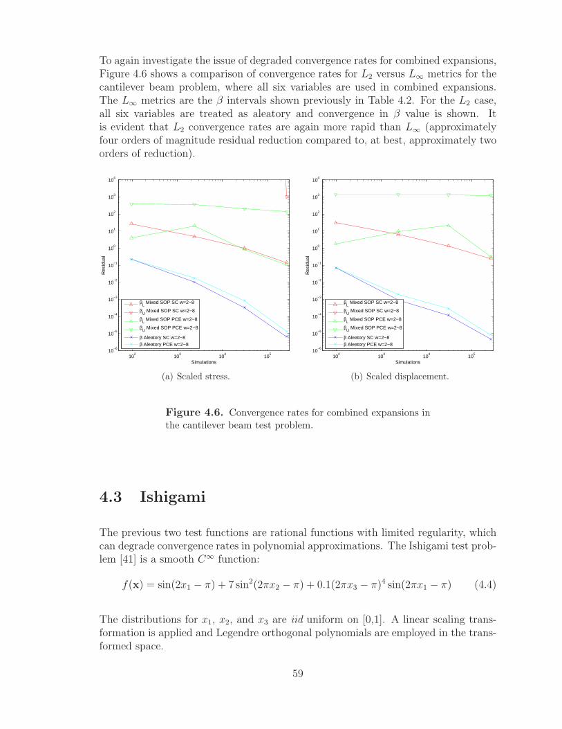
To again investigate the issue of degraded convergence rates for combined expansions,Figure 4.6 shows a comparison of convergence rates for L2 versus L∞ metrics for thecantilever beam problem, where all six variables are used in combined expansions.The L∞ metrics are the β intervals shown previously in Table 4.2. For the L2 case,all six variables are treated as aleatory and convergence in β value is shown. Itis evident that L2 convergence rates are again more rapid than L∞ (approximatelyfour orders of magnitude residual reduction compared to, at best, approximately twoorders of reduction).

102

103

104

105

10−6

10−5

10−4

10−3

10−2

10−1

100

101

102

103

104

Simulations

Res

idua

l


βU



βU



(a) Scaled stress.

102

103

104

105

10−6

10−5

10−4

10−3

10−2

10−1

100

101

102

103

104

Simulations

Res

idua

l


βU



βU



(b) Scaled displacement.

Figure 4.6. Convergence rates for combined expansions inthe cantilever beam test problem.

4.3 Ishigami

The previous two test functions are rational functions with limited regularity, whichcan degrade convergence rates in polynomial approximations. The Ishigami test prob-lem [41] is a smooth C∞ function:

f(x) = sin(2x1 − π) + 7 sin2(2πx2 − π) + 0.1(2πx3 − π)4 sin(2πx1 − π) (4.4)

The distributions for x1, x2, and x3 are iid uniform on [0,1]. A linear scaling trans-formation is applied and Legendre orthogonal polynomials are employed in the trans-formed space.

59


In Figure 4.7, a comparison of convergence rates is shown for L2 versus L∞ metrics forthe Ishigami problem, where all three variables are used in combined expansions. Forthe L2 case, all three variables are treated as aleatory and convergence in β value isshown. For the L∞ case, x1 is treated as an epistemic interval while x2 and x3 remainaleatory, and convergence in the epistemic interval bounds for the aleatory β statisticis shown (in this case, all interval estimation is just post-processing of the combinedexpansion). It is evident that L2 and L∞ convergence rates are quite similar for thissmooth C∞ function: SC convergence plots are nearly on top of one another and thePCE convergence plots have a fairly consistent residual gap throughout. Thus, itappears that point-wise L∞ accuracy can be achieved at similar cost to L2 accuracy,provided that the function is sufficiently smooth.

101

102

103

104

105

10−14

10−12

10−10

10−8

10−6

10−4

10−2

100

Simulations

Res

idua

l

βL Mixed SOP SC w=2−8 CC

βU

Mixed SOP SC w=2−8 CC

βL Mixed SOP PCE w=2−14 GL

βU

Mixed SOP PCE w=2−14 GL

β Aleatory SC w=2−8 CCβ Aleatory PCE w=2−14 GL

Figure 4.7. Convergence rates for combined expansions inthe Ishigami test problem.

60

4.4 Sobol’s g function

At the opposite end of the smoothness spectrum, Sobol’s g-function [41] is C0 withthe absolute value contributing a slope discontinuity at the center of the domain:

f(x) = 25

∏

j=1

|4xj − 2| + aj

1 + aj; a = [0, 1, 2, 4, 8] (4.5)

The distributions for xj for j = 1, 2, 3, 4, 5 are iid uniform on [0,1]. A linear scalingtransformation is applied and Legendre orthogonal polynomials are employed in thetransformed space.

Without any mitigation measures (e.g., discretization of the random domain), weexpect for smooth global polynomial approximations to exhibit Gibbs phenomenanear the discontinuity, resulting in slow convergence in L2 measures.


In Figure 4.8, a comparison of convergence behavior is shown for L2 versus L∞ metricsfor the Sobol g-function problem, where all five variables are used in combined expan-sions. Since convergence rates are relatively poor in this case, an overkill referencesolution is not available and residuals cannot be reliably estimated. Rather, the val-ues of the statistics are plotted directly and general convergence trends are inferred.For the L2 case, all five variables are treated as aleatory and slow convergence in β

value is apparent with agreement between the PCE and SC estimates. For the L∞case, x1 and x2 are treated as epistemic intervals while x3 through x5 remain aleatoryand the resulting L∞ intervals can be seen to be neither converging nor consistentbetween PCE and SC. Thus, one can infer that point-wise L∞ accuracy may not beattainable for nonsmooth functions. In fact, one might anticipate divergence in someL∞ metrics in the presence of Gibbs oscillations of increasing amplitude.

61

102

103

104

105

106

−2

0

2

4

6

8

10

12

Simulations

Sta

tistic

val

ue

βL Mixed SOP SC w=2−8 CC

βU

Mixed SOP SC w=2−8 CC

βL Mixed SOP PCE w=2−10 GL

βU

Mixed SOP PCE w=2−10 GL

β Aleatory SC w=2−10 CCβ Aleatory PCE w=2−10 GL

Figure 4.8. Convergence for combined expansions in theSobol g-function test problem.

62

Chapter 5

Accomplishments and Conclusions

The goal of this milestone was to develop second-order probability approaches formixed aleatory-epistemic uncertainty quantification that can be more accurate (viaprecise bounds from optimizers) and more efficient (via exponential convergencerates from stochastic expansion methods) than nested sampling. Computational ex-periments have demonstrated that the coupling of local gradient-based and globalnongradient-based optimizers with nonintrusive polynomial chaos and stochastic col-location expansion methods is highly effective, and provides interval bounds on statis-tics for two model problems using O(102) −O(103) simulations that are significantlymore accurate than those obtainable from O(108) simulations in the traditional nestedsampling approach.

5.1 Observations on optimization-based interval es-

timation

While there are many different possible optimization algorithms that could be ex-amined, we focused on two: the global nongradient-based EGO algorithm, based onsuccessive refinement of Gaussian process surrogate models, and the local gradient-based NPSOL algorithm, employing stochastic sensitivities. Key considerations inthese selections include data reuse between interval minimization and maximizationsteps, support for nonsmooth and/or multimodal response functions, and scalabilityto large numbers of epistemic parameters. For the first two considerations, globalmethods are more effective, and for the last consideration, local methods are moreeffective. Table 5.1 provides additional details.

Additional observations for optimization-based interval estimation include:

• In addition to EGO, global methods supporting data reuse include DIRECT(reuse of box partitioning data within minimization and maximization Paretofrontiers) and other global surrogate-based approaches. DIRECT will be of fu-ture interest since it avoids potential issues with Gaussian process ill-conditioning,scaling, etc.

63

Table 5.1. Comparison of local and global optimization-based interval estimation.

AlgorithmType Pro Con

Global

• Global data reuse

• Responses may be multi-modal and nonsmooth

• Gradients not required

• Supports only up to O(101)epistemic variables

• “Soft” convergence is not asprecise

Local

• Epistemic dimension may belarge scale

• “Hard” convergence at KKTpoints to tight precision

• Only initial point reuse

• Response should be smoothand unimodal

• Gradients should be accurateand reliable

• Another attractive future method would be EGO employing gradients (utilizingthe concept of “gradient-based kriging”). This would retain the desirable globalidentification properties of EGO, but take advantage of the stochastic sensitivitycapabilities to improve the accuracy of the Gaussian process models in orderto accelerate the epistemic search. This would likely also mitigate epistemicdimensionality issues to some degree.

5.2 Observations on stochastic expansions

This report has included investigation of the relative performance of non-intrusivegeneralized polynomial chaos and Lagrange interpolation-based stochastic colloca-tion methods applied to algebraic benchmark problems with known solutions. Theprimary distinction between these methods is that PCE must estimate coefficients fora known basis of orthogonal polynomials (using sampling, linear regression, tensor-product quadrature (TPQ), or Smolyak sparse grids (SSG)) whereas SC must forman interpolant for known coefficients (using TPQ or SSG).

Performance between these methods is shown to be very similar and both demonstrateimpressive efficiency relative to Monte Carlo sampling methods and impressive accu-racy relative to local reliability methods, thereby providing a more effective balance ofaccuracy and efficiency over current production UQ methods for aleatory uncertainty.When a difference is observed between traditional PCE and SC using the same col-location point sets, SC has been the consistent winner, typically manifesting in thereduction of the required integration by one order or level. This difference can be

64

attributed at least in part to expansion/integration synchronization issues with PCE,motivating approaches for tailoring of chaos expansions that closely synchronize withnumerical integration schemes:

• For the case of TPQ, tailored tensor-product PCE is shown to perform iden-tically to SC such that the performance gap is completely eliminated. Bothmethods consistently outperform traditional total-order PCE. However, TPQapproaches only outperform SSG approaches for the lowest dimensional prob-lems.

• For problems with greater than two dimensions, SSG approaches are shown tooutperform TPQ approaches.

– For SSG, selection of a synchronized PCE formulation is nontrivial andthe tailored total-order PCE approach, which computes the maximal total-order expansion that can be resolved by a particular SSG, is shown to bemore rigorous and reliable than heuristics and eliminates inefficiency dueto trial and error.

– A significant performance gap relative to SC with SSG still remains forthe case of nonlinear growth rules, but replacement of these rules withlinear ones (for Gaussian quadratures that are at most weakly nested)reduces the set of resolvable monomials that do not appear in the total-order expansion, resulting in a further reduction of the performance gap.

While efforts in tailoring the form of the PCE can reduce and in some cases eliminatethe performance gap with SC, no nonintrusive PCE approach has been shown tooutperform SC when using the same set of collocation points. Rather, usage ofPCE remains motivated by other considerations, in particular its greater flexibility incollocation point selection and coefficient estimation approaches. In particular, PCEallows for:

• usage of unstructured/random collocation point sets (with random samplingand linear regression approaches) that can support greater simulation fault tol-erance

• Genz cubature grids that support more optimal numerical integration than SSG,at least for low order rules

• linear regression approaches that may enable approximate resolution of higherrandom dimensions and higher expansion orders than SSG approaches

In addition, a guarantee of positive expansion variance is a feature of PCE not pro-vided by SC, and this can be particularly important when computing intervals onvariance-related metrics. Thus, PCE and SC provide their own sets of strengths

65

and weaknesses and selection between the two approaches remains dependent on theefficiency and flexibility requirements of specific applications.

Another type of stochastic expansion tailoring that was explored is the selection ofbasis polynomials along with their associated Gauss points and weights. For inde-pendent random variables with density functions outside of the Askey family, twoapproaches are supported: (1) nonlinear variable transformation of the non-Askeydensity function to the most similar Askey density, or (2) numerical generation ofpolynomials that are orthogonal with respect to an arbitrary density. Mixed resultswere shown in which simple polynomial response functions showed clear benefit fromthe numerically-generated basis, but rational response functions with non-Askey vari-ables in the denominator required lower order response expansions using the variabletransformation approach. It is expected that the special conditions met in the ratio-nal function examples will be the exception rather than the rule, and that numericallygenerated polynomials will generally be preferred; however, additional computationalexperience is needed.

5.3 Observations on second-order probability

The preferred UQ approaches identified in stochastic expansion computational exper-iments are (1) SC with TPQ for low dimensions and linear growth SSG for high di-mensions, and (2) tailored PCE with TPQ for low dimensions and either linear growthSSG or linear regression for high dimensions. These approaches are carried forward inepistemic interval estimation studies employing two stochastic expansion/sensitivityapproaches (aleatory and combined expansions) and two optimization approaches(local gradient-based and global nongradient-based).

For the expansion/sensitivity approaches, the first approach forms expansions onlyover the aleatory uncertain variables for both the response values and the responsesensitivities. It is a first-order technique requiring accurate derivatives of the responsefunction with respect to the epistemic variables; derivatives of aleatory statisticswith respect to epistemic variables are formed based on aleatory expectations ofepistemic response derivatives. The second approach forms combined expansionsof response values over both the aleatory and epistemic variables. It is a zeroth-order technique; derivatives of statistics are formed by differentiating the polynomialrelationship between the aleatory statistics (formed from integrating out the aleatoryexpansion terms) and the remaining epistemic expansion terms. While it is shownthat both approaches are capable of exact results, computational experiments indicatethat the former aleatory expansion approach is generally more efficient and reliable(so long as the underlying epistemic response derivatives are reliable) for use withinoptimization-based interval estimation. This appears to be due to two factors:

1. Convergence rates can be degraded when computing point-wise L∞ metrics

66

(minima and maxima) from stochastic expansions. Rational, infinitely differen-tiable, and discontinuous response functions were investigated, and only for thesmooth C∞ case were the L2 and L∞ convergence rates comparable. Thus, forgeneral functions that may not be infinitely differentiable, it appears preferableto restrict stochastic expansion approximation to dimensions requiring aleatoryL2 metrics (mean, variance, probability) and to handle dimensions requiringepistemic L∞ metrics (interval bounds) through other means (i.e., direct opti-mization without stochastic expansion approximation).

2. The previous statement assumes sparse interrogation of the epistemic space byefficient local and global optimizers. For second-order probability in which asingle interval is computed for each response function, the number of epistemicpoint evaluations is relatively small, such that the cost of resolving the aleatorystatistics for only selected instances of the nonprobabilistic parameters (aleatoryexpansions) one at a time may tend to be more efficient than attempting toglobally resolve these statistics for all values of the nonprobabilistic parameters(combined expansions) all at once. For more finely-discretized epistemic analy-ses such as Dempster-Shafer theory of evidence, the interrogation requirementsfor the epistemic space may grow substantially, such that combined expansionsmay prove useful in this case. Moreover, development of more rapidly con-verging approaches in L∞ for combined expansions may be possible and maybecome motivated by the Dempster-Shafer use case.

For the optimization approaches, the first approach employs the stochastic sensitiv-ities from the aleatory or combined expansions to perform a local gradient-basedsearch for minima and maxima of the response metrics over the epistemic parame-ter ranges. As for all local gradient-based methods (and as discussed previously inSection 5.1), it requires response metrics that are smooth and unimodal over the epis-temic space to be effective. The second approach employs a nongradient-based globalsearch for minima and maxima. It is a zeroth-order technique that only requiresaccurate predictions of the aleatory statistic values over the epistemic space. In boththe short column and cantilever beam test problems, the aleatory statistics behavedmonotonically over the epistemic parameter ranges, such that both local and globalsearches located the same solutions. For the short column problem, the expense ofthe best local and global approaches was comparable (341 limit state function andgradient evaluations for NPSOL versus 403 limit state function evaluations for EGO);whereas in the cantilever beam problem, the local search displayed greater efficiency(245 stress and 147 displacement function/gradient evaluations for NPSOL versus931 stress and 1960 displacement function evaluations for EGO). Overall, these ex-periments are consistent with the anticipated trade-off between the scalability andefficiency of local approaches and the robustness of global approaches for nonsmooth,multimodal problems; although additional experimentation will help quantify theseeffects more precisely. Relative to nested sampling in the short column problem,our new approaches reduce expense by greater than five orders of magnitude whileachieving more precise results (five to six digits of accuracy in the output intervals

67

instead of only one to three digits). And in the cantilever beam problem, our newapproaches are again much more efficient, reducing expense by five to six orders ofmagnitude, while again achieving more precise results, four to six digits of accuracyinstead of only zero to two.

Additional observations include:

• Since the relative computational expense of the local and global optimizationapproaches is only relevant for point-wise aleatory expansions, the greater al-gorithmic robustness of the global EGO approach is recommended for intervalestimation on combined expansions, since these expansions only involve inex-pensive post-processing in either optimization case.

• Overall, the most effective SOP approach was SC using linear SSG with expan-sions formed only over the aleatory variables for each instance of the epistemicvariables. In this case, the selection between local and global optimization isrelevant and should be based on the efficiency, scalability, and algorithmic ro-bustness concerns previously identified.

• This report explored global-global and local-global combinations for outer-innernested loops to support either algorithmic robustness or scalability with respectto epistemic dimension. To sacrifice algorithmic robustness in exchange for scal-ability with respect to aleatory dimension, global stochastic expansions could bereplaced with local gradient-based reliability methods for aleatory UQ. Overall,global-global, local-global, global-local, and local-local combinations are all eas-ily configured in DAKOTA, allowing one to tailor the approach for robustnessor scalability separately within epistemic and aleatory domains.

• In future research, dimension-adaptive stochastic expansion methods will bet-ter address the curse of dimensionality, allowing usage of global machinery atreduced cost for larger problems.

5.4 Accomplishments, Capability Development, and

Deployment

This milestone crosscuts multiple centers, drawing on capabilities for uncertaintyanalysis from DAKOTA (1410), device and circuit simulation from Charon and Xyce(1430), and QASPR data analysis, model development, and program relevance (0410,1340, 1430, 1540). Many new capabilities have been developed and tested within theDAKOTA code for use in this milestone, including:

• stochastic expansions over nonprobabilistic dimensions

68

• stochastic sensitivity analysis capabilities for aleatory and combined expansions

• local gradient-based and global nongradient-based optimization approaches toepistemic interval estimation with data reuse among minimization and maxi-mization solves

• nested analyses within second-order probability and Dempster-Shafer methodsfor mixed aleatory-epistemic UQ

New capabilities developed for this milestone are being inserted into production UQanalysis procedures for current and future radiation effects studies, and this trend isexpected to continue with V&V efforts in other program areas.

69

References

[1] M. Abramowitz and I. A. Stegun. Handbook of Mathematical Functions withFormulas, Graphs, and Mathematical Tables. Dover, New York, 1965.

[2] R. Askey and J. Wilson. Some basic hypergeometric polynomials that generalizejacobi polynomials. In Mem. Amer. Math. Soc. 319, Providence, RI, 1985. AMS.

[3] V. Barthelmann, E. Novak, and K. Ritter. High dimensional polynomial interpo-lation on sparse grids. Adv. Comput. Math., 12(4):273–288, 2000. Multivariatepolynomial interpolation.

[4] B. J. Bichon, M. S. Eldred, L. P. Swiler, S. Mahadevan, and J. M. McFarland.Efficient global reliability analysis for nonlinear implicit performance functions.AIAA Journal, 46(10):2459–2468, 2008.

[5] G. E. P. Box and D. R Cox. An analysis of transformations. J. Royal Stat. Soc.,26:211–252, 1964.

[6] X. Chen and N .C. Lind. Fast probability integration by three-parameter normaltail approximation. Struct. Saf., 1:269–276, 1983.

[7] A. Der Kiureghian and P. L. Liu. Structural reliability under incomplete proba-bility information. J. Eng. Mech., ASCE, 112(1):85–104, 1986.

[8] M. S. Eldred. Recent advances in non-intrusive polynomial chaos and stochasticcollocation methods for uncertainty analysis and design. In Proceedings of the11th AIAA Nondeterministic Approaches Conference, number AIAA-2009-2274,Palm Springs, CA, May 4–7 2009.

[9] M. S. Eldred, B. M. Adams, K. Haskell, W. J. Bohnhoff, J. P. Eddy, D. M.Gay, W. E. Hart, P. D. Hough, T. G. Kolda, L. P. Swiler, and J.-P. Watson.DAKOTA, a multilevel parallel object-oriented framework for design optimiza-tion, parameter estimation, uncertainty quantification, and sensitivity analysis:Version 4.2 users manual. Technical Report SAND2006-6337, Sandia NationalLaboratories, Albuquerque, NM, 2008.

[10] M. S. Eldred, H. Agarwal, V. M. Perez, S. F. Wojtkiewicz, Jr., and J. E. Re-naud. Investigation of reliability method formulations in DAKOTA/UQ. Struc-ture & Infrastructure Engineering: Maintenance, Management, Life-Cycle De-sign & Performance, 3(3):199–213, 2007.

71

[11] M. S. Eldred and B. J. Bichon. Second-order reliability formulations inDAKOTA/UQ. In Proceedings of the 47th AIAA/ASME/ASCE/AHS/ASCStructures, Structural Dynamics and Materials Conference, number AIAA-2006-1828, Newport, RI, May 1–4 2006.

[12] M. S. Eldred and J. Burkardt. Comparison of non-intrusive polynomial chaosand stochastic collocation methods for uncertainty quantification. In Proceedingsof the 47th AIAA Aerospace Sciences Meeting and Exhibit, number AIAA-2009-0976, Orlando, FL, January 5–8, 2009.

[13] M. S. Eldred and D. M. Dunlavy. Formulations for surrogate-based optimizationwith data fit, multifidelity, and reduced-order models. In Proceedings of the 11thAIAA/ISSMO Multidisciplinary Analysis and Optimization Conference, numberAIAA-2006-7117, Portsmouth, VA, September 6–8 2006.

[14] M. S. Eldred, C. G. Webster, and P. Constantine. Design under uncertainty em-ploying stochastic expansion methods. In Proceedings of the 12th AIAA/ISSMOMultidisciplinary Analysis and Optimization Conference, number AIAA-2008-6001, Victoria, British Columbia, September 10–12, 2008.

[15] M. S. Eldred, C. G. Webster, and P. Constantine. Evaluation of non-intrusiveapproaches for wiener-askey generalized polynomial chaos. In Proceedings of the10th AIAA Nondeterministic Approaches Conference, number AIAA-2008-1892,Schaumburg, IL, April 7–10 2008.

[16] P. Frauenfelder, C. Schwab, and R. A. Todor. Finite elements for elliptic problemswith stochastic coefficients. Comput. Methods Appl. Mech. Engrg., 194(2-5):205–228, 2005.

[17] J. M Gablonsky. An implementation of the direct algorithm. Technical ReportTechnical Report CRSC-TR98-29, Center for Research in Scientific Computa-tion, North Carolina State University, Chapel Hill, NC, August 1998.

[18] W. Gautschi. Orthogonal Polynomials: Computation and Approximation. OxfordUniversity Press, New York, 2004.

[19] T. Gerstner and M. Griebel. Numerical integration using sparse grids. Numer.Algorithms, 18(3-4):209–232, 1998.

[20] R. G. Ghanem. private communication.

[21] P. E. Gill, W. Murray, M. A. Saunders, and M. H. Wright. User’s guide for npsol5.0: A fortran package for nonlinear programming. Technical Report SOL 86-1,System Optimization Laboratory, Stanford University, Stanford, CA, RevisedJuly 1998.

[22] G. H.. Golub and J. H. Welsch. Caclulation of gauss quadrature rules. Mathe-matics of Computation, 23(106):221–230, 1969.

72

[23] J. C. Helton. Conceptual and computational basis for the quantification of mar-gins and uncertainty. Technical Report SAND2009-3055, Sandia National Lab-oratories, Albuquerque, NM, July 2009.

[24] J. C. Helton, J. D. Johnson, and W. L. Oberkampf. An exploration of alternativeapproaches to the representation of uncertainty in model predictions. ReliabilityEngineering and System Safety, 85:39–71, 2004.

[25] J. C. Helton, J. D. Johnson, W. L. Oberkampf, and C. B. Storlie. A sampling-based computational strategy for the representation of epistemic uncertainty inmodel predictions with evidence theory. Computer Methods in Applied Mechanicsand Engineering, 196:3980–3998, 2007.

[26] S. Hosder, R. W. Walters, and M. Balch. Efficient sampling for non-intrusivepolynomial chaos applications with multiple uncertain input variables. In Pro-ceedings of the 48th AIAA/ASME/ASCE/AHS/ASC Structures, Structural Dy-namics, and Materials Conference, number AIAA-2007-1939, Honolulu, HI,April 23–26, 2007.

[27] D. Huang, T. T. Allen, W. I. Notz, and N. Zang. Global optimization of stochas-tic black-box systems via sequential kriging meta-models. J. Global Optimization,34:441–466, 2006.

[28] D. Jones, M. Schonlau, and W. Welch. Efficient global optimization of expensiveblack-box functions. J. Global Optimization, 13:455–492, 1998.

[29] N. Kuschel and R. Rackwitz. Two basic problems in reliability-based structuraloptimization. Math. Method Oper. Res., 46:309–333, 1997.

[30] J. D. Martin and T. W. Simpson. Use of kriging models to approximate deter-ministic computer models. AIAA Journal, 43(4):853–863, 2005.

[31] J. M. McFarland. Uncertainty Analysis for Computer Simulations through Vali-dation and Calibration. PhD thesis, Vanderbilt University, Nashville, TN, May2008.

[32] J. C. Meza. OPT++: An object-oriented class library for nonlinear optimization.Technical Report SAND94-8225, Sandia National Laboratories, Albuquerque,NM, March 1994.

[33] F. Nobile, R. Tempone, and C. G. Webster. An anisotropic sparse grid stochasticcollocation method for partial differential equations with random input data.SIAM J. on Num. Anal., 2008. To appear.

[34] F. Nobile, R. Tempone, and C. G. Webster. A sparse grid stochastic collocationmethod for partial differential equations with random input data. SIAM J. onNum. Anal., 2008. To appear.

73

[35] R. Rackwitz and B. Fiessler. Structural reliability under combined random loadsequences. Comput. Struct., 9:489–494, 1978.

[36] M. T. Reagan, H. N. Najm, P. P. Pebay, O. M. Knio, and R. G. Ghanem.Quantifying uncertainty in chemical systems modeling. Int. J. Chem. Kinet.,37:368–382, 2005.

[37] M. Rosenblatt. Remarks on a multivariate transformation. Ann. Math. Stat.,23(3):470–472, 1952.

[38] J. Sacks, S. B. Schiller, and W. Welch. Design for computer experiments. Tech-nometrics, 31:41–47, 1989.

[39] I.C. Simpson. Numerical integration over a semi-infinite interval, using the log-normal distibution. Numerische Mathematik, 31, 1978.

[40] S.A. Smolyak. Quadrature and interpolation formulas for tensor products ofcertain classes of functions. Dokl. Akad. Nauk SSSR, 4:240–243, 1963.

[41] C. B. Storlie, L. P. Swiler, J. C. Helton, and C. J. Sallaberry. Implementationand evaluation of nonparametric regression procedures for sensitivity analysis ofcomputationally demanding models. Reliability Engineering and System Safety,94:1735–1763, 2009.

[42] B. Sudret. Global sensitivity analysis using polynomial chaos expansions. Reli-ability Engineering and System Safety, 93, 2008.

[43] R. Sues, M. Aminpour, and Y. Shin. Reliability-based multidisci-plinary optimization for aerospace systems. In Proceedings of the 42rdAIAA/ASME/ASCE/AHS/ASC Structures, Structural Dynamics, and Materi-als Conference, number AIAA-2001-1521, Seattle, WA, April 16–19, 2001.

[44] L. P. Swiler, T. L. Paez, and R. L. Mayes. Epistemic uncertainty quantifica-tion tutorial. In Proceedings of the IMAC XXVII Conference and Exposition onStructural Dynamics, number paper 294, Orlando, FL, February 2009.

[45] L. P. Swiler, T. L. Paez, R. L. Mayes, and M. S. Eldred. Epis-temic uncertainty in the calculation of margins. Proceedings of the 50thAIAA/ASME/ASCE/AHS/ASC Structures, Structural Dynamics, and Materi-als Conference, (AIAA-2009-2249), May 4-7, 2009.

[46] G. Tang, G. Iaccarino, and M. S. Eldred. Global sensitivity analysis for stochasticcollocation expansion. In abstract submitted for 12th AIAA Non-DeterministicApproaches Conference, Orlando, FL, April 12–15, 2010.

[47] G. Tang, L. P. Swiler, and M. S. Eldred. Using stochastic expansion methodsin evidence theory for mixed aleatory-epistemic uncertainty quantification. Inabstract submitted for 12th AIAA Non-Deterministic Approaches Conference,Orlando, FL, April 12–15, 2010.

74

[48] R. W. Walters. Towards stochastic fluid mechanics via polynomial chaos. InProceedings of the 41st AIAA Aerospace Sciences Meeting and Exhibit, numberAIAA-2003-0413, Reno, NV, January 6–9, 2003.

[49] G. W. Wasilkowski and H. Wozniakowski. Explicit cost bounds of algorithms formultivariate tensor product problems. Journal of Complexity, 11:1–56, 1995.

[50] N. Wiener. The homogoeneous chaos. Amer. J. Math., 60:897–936, 1938.

[51] J. A. S. Witteveen and H. Bijl. Modeling arbitrary uncertainties using gram-schmidt polynomial chaos. In Proceedings of the 44th AIAA Aerospace SciencesMeeting and Exhibit, number AIAA-2006-0896, Reno, NV, January 9–12 2006.

[52] Y.-T. Wu, Y. Shin, R. Sues, and M. Cesare. Safety-factor based ap-proach for probability-based design optimization. In Proceedings of the 42rdAIAA/ASME/ASCE/AHS/ASC Structures, Structural Dynamics, and Materi-als Conference, number AIAA-2001-1522, Seattle, WA, April 16–19, 2001.

[53] Y.-T. Wu and P. H. Wirsching. A new algorithm for structural reliability esti-mation. J. Eng. Mech., ASCE, 113:1319–1336, 1987.

[54] D. Xiu and J.S. Hesthaven. High-order collocation methods for differential equa-tions with random inputs. SIAM J. Sci. Comput., 27(3):1118–1139 (electronic),2005.

[55] D. Xiu and G. M. Karniadakis. The wiener-askey polynomial chaos for stochasticdifferential equations. SIAM J. Sci. Comput., 24(2):619–644, 2002.

75

DISTRIBUTION:

1 Juan J. AlonsoDurand Building, Room 365Department of Aeronautics &AstronauticsStanford UniversityStanford, CA 94305

1 Barron J. BichonResearch EngineerSouthwest Research Institute6220 Culebra RoadP.O. Drawer 28510San Antonio, Texas 78228-0510

1 Krzysztof J. FidkowskiDepartment of Aerospace Engi-neeringThe University of Michigan3029 FXB BuildingAnn Arbor, MI 48109

1 Roger Ghanem254C Kaprielian HallDept. of Civil Engineering3620 S. Vermont Ave.University of Southern Califor-niaLos Angeles, CA 90089-2531

1 Raphael HaftkaDept. of Aerospace and Mechan-ical Engineering and EngineeringScienceP.O. Box 116250University of FloridaGainesville, FL 32611-6250

1 Gianluca IaccarinoBldg 500, 500-I, MechanicalEngineering DepartmentInstitute for ComputationalMathematical EngineeringStanford UniversityStanford, CA 94305-3030

76

1 Sankaran MahadevanDepartment of Civil and Envi-ronmental EngineeringBox 1831, Station BVanderbilt UniversityNashville, TN 37235

1 Kurt MauteDepartment of Aerospace Engi-neering SciencesUniversity of Colorado at Boul-derRoom ECAE 183, Campus Box429Boulder, Colorado 80309-0429

1 John E. RenaudUniversity of Notre DameAerospace and Mechanical Engi-neering365 Fitzpatrick HallNotre Dame, IN 46556-5637

1 Christopher J. Roy215 Randolph HallVirginia Polytechnic Instituteand State UniversityBlacksburg, Virginia 24061-0203

1 Karen E. WillcoxDepartment of Aeronautics &AstronauticsMassachusetts Institute of Tech-nology77 Massachusetts AveRoom 37-447Cambridge, MA 02139

1 Steven F. Wojtkiewicz, Jr.Department of Civil EngineeringUniversity of Minnesota500 Pillsbury Drive S.E.Minneapolis, MN 55455-0116

1 Dongbin XiuMath DepartmentMath 434Purdue UniversityWest Lafayette, IN 47907

77

5 Lawrence Livermore NationalLaboratory7000 East Ave.P.O. Box 808Livermore, CA 94550Attn: Scott Brandon, MS L-023

Frank Graziani, MS L-095Richard Klein, MS L-023Jim McEnerney, MS L-023Charles Tong, MS L-560

3 Los Alamos National LaboratoryMail Station 5000P.O. Box 1663Los Alamos, NM 87545Attn: Marc Anderson, MS T080

Scott Doebling, MS T080Francois Hemez, MS T006

1 MS 0316J. P. Castro, 1437

1 MS 0316R. J. Hoekstra, 1437

1 MS 0316E. R. Keiter, 1437

1 MS 0316B. S. Paskaleva, 1437

1 MS 0321J. S. Peery, 1400

1 MS 0352C. E. Hembree, 1344

1 MS 0370T. G. Trucano, 1411

1 MS 0378A. M. Robinson, 1431

1 MS 0380G. M. Reese, 1542

1 MS 0380D. E. Womble, 1540

1 MS 0382B. Carnes, 1543

78

1 MS 0492T. D. Brown, 0411

2 MS 0776J. C. Helton, 1544

1 MS 0828A. R. Black, 1544

1 MS 0828K. J. Dowding, 1544

1 MS 0828A. A. Giunta, 1544

1 MS 0828R. G. Hills, 1544

1 MS 0828M. Pilch, 1551

1 MS 0828J. R. Red-Horse, 1544

1 MS 0828V. J. Romero, 1544

1 MS 0829B. M. Rutherford, 0415

1 MS 0836M. M. Hopkins, 1514

1 MS 0836P. K. Notz, 1514

1 MS 0847R. V. Field, 1526

1 MS 1318B. M. Adams, 1411

1 MS 1318K. F. Alvin, 1414

3 MS 1318M. S. Eldred, 1411

1 MS 1318B. A. Hendrickson, 1410

1 MS 1318R. P. Pawlowski, 1414

79

1 MS 1318E. T. Phipps, 1411

1 MS 1318J. R. Stewart, 1411

3 MS 1318L. P. Swiler, 1411

1 MS 1320S. S. Collis, 1416

1 MS 1322J. B. Aidun, 1435

1 MS 1415S. M. Meyers, 1110

1 MS 9051B. J. Debusschere, 8351

1 MS 9051H. N. Najm, 8351

1 MS 9159H. R. Ammerlahn, 8962

1 MS 9159G. A. Gray, 8964

1 MS 9159P. D. Hough, 8964

1 MS 0899Technical Library, 9536(electronic copy)

80

efﬁcient algorithms for mixed aleatory-epistemic ... · eﬃcient algorithms for mixed...

Documents