eecs 216 winter 2008 solutions lab 3: am radio …...eecs 216 winter 2008 solutions lab 3: am radio...

EECS 216 Winter 2008 SOLUTIONS

Lab 3: AM Radio

Part I: Intro & Pre-lab Assignmentc©Kim Winick 2008

1 Introduction

1.1 A Bit of History

The transmission and storage of information are vital functions of a modern society. The algorithmic anddevice technologies supporting these functions continue to advance at a rapid pace. Use of the internet andwireless services (e.g., cellphones) is now pervasive, and other forms of communications, such as digital radioand high definition television, are growing in popularity.

This laboratory is aimed at the following question - how can we transmit information wirelessly? Toaddress this question, we need to understand something about the propagation of electromagnetic waves1

and how to build a transmitter and receiver that will have sufficient power and sensitivity, respectively.Given the prevalence of wireless devices today, you may find it very surprising that the invention of the radiowas a nontrivial matter. Well, it was not easy!

In the beginning, one used wires. The age of electronic communication arguably began in 1830 withthe invention of the telegraph2. In 1844, news was conveyed for the first time using the telegraph, and thetelegraph remained a popular means of sending information until the middle of the twentieth century. In the1870s, voice transmission began with the introduction of the telephone, which was independently invented byElisha Gray and Alexander Graham Bell. Both the telegraph and telephone were revolutionary inventions,but both require that the transmitter and receiver be physically connected via a wire.

It was not until the late 1800s that the theory of electromagnetics was developed through the effortsof Michael Faraday, James Clerk Maxwell and others. In 1887, Heinrich Hertz confirmed the predictionsof Maxwell’s theory by transmitting and detecting electromagnetic waves (i.e., radio waves). Although theapparatus used by Hertz was quite crude by today’s standards, his work launched the modern era of wirelesscommunications. It is a quirky bit of history that Hertz failed to fully appreciate the practical significanceof his own scientific work! He stated that “It’s of no use whatsoever. . . this is just an experiment thatproves Maestro Maxwell was right – we just have these mysterious electromagnetic waves that we cannotsee with the naked eye. But they are there.” He went on to say “I do not think that the wireless wavesI have discovered will have any practical applications.” Obviously Hertz was a far better scientist thanbusinessman!

In Hertz’s experiment, batteries were used to charge up a large capacitor. After charging, the capacitorwas connected to pair of wires whose opposite ends were placed in very close proximity, with only a small airgap between them. The voltage on the capacitor produced a strong electric field in the small air gap region,which in turn caused the air molecules inside the gap to ionize. In their ionized state, these molecules conductelectricity, and a spark of short duration was produced inside the gap when the capacitor discharged. Thespark current was significant, since the large capacitor stored a substantial amount of charge. This dischargephenomenon is similar to that of a lightning bolt. The spark produces an electromagnetic (EM) wave thatpropagates away from the transmitter. As observed by Hertz, the presence of this wave can be detected at

1We take as a given from everyday experience that sound waves simply don’t travel far enough without dissipating, and thatmultiple people talking in a room leads to interference!

2The original digital communication system? Dots and dashes!

1

Lab 3 SOLUTIONS AM Radio

a distant point, since this wave will induce a small burst of current in a distant loop of wire. By varyingthe time delay between successive transmitted bursts, Hertz’s system would be used by others to transmitinformation wirelessly from one point to another.

In 1894 an improved detection device, known as a cohere, was developed by Oliver Lodge, AlexanderPopov and Edouard Branly. This device consisted of a glass tube filled with metal filings. With a wireinserted into each end of the tube, the device functioned as a resistor. The value of the resistance, however,was found to change (in particular, decrease) in the presence of an electromagnetic wave. A circuit was builtusing this device that produced an increase in current in the presence of a received EM burst. The coherenever worked particularly well, but Guglielmo Marconi used a spark gap transmitter, a telegraph key and acohere to demonstrate transatlantic telegraphy in 1901. The short bursts of EM waves produced by a sparkgap transmitter were never suitable for voice transmission.

The spark gap transmission scheme turns out to suffer from a number of serious drawbacks. First, itis not suitable for voice transmission, only telegraphy. Second, it is difficult to efficiently couple the sparkenergy into an antenna for transmission. Third, the pulsed EM energy does not propagate well over longdistances. Fourth, the pulse energy is distributed over a very wide spectral band, and as a consequenceit impossible for the receiver to do station selection when multiple transmitters are operating (since all ofthe signals will occupy the same spectral band). Near the very end of the 19th century, Nikola Tesla (hisbust is displayed in the EECS atrium by the elevators) developed a device called the RF alternator thatcould be used together with tuned LC circuits to generate a quasi-sinusoidal carrier, thereby reducing thespectral bandwidth of the signal and permitting more efficient coupling to an antenna. The availability ofhigh quality sinusoidal sources (e.g., oscillators), however, would have to await the development of vacuumtubes.

The early receivers also had their problems. They lacked sensitivity and consequently suffered fromnoise. A high quality nonlinear component was not yet available to permit efficient envelope detection,and the receivers had no mechanism for station selection even if multiple transmitters had been able tooperate on different frequency bands. The first experimental wireless broadcast of voice (and music too) wasdemonstrated by Reginald Fessenden on December 24, 1906. His transmitter used a spark gap unit drivenby an RF alternator that produced a quasi-sinusoidal carrier. The carrier was then amplitude modulatedby placing a microphone in series with the antenna. The receiver contained a resonant circuit with a peakresponse tuned to the carrier frequency followed by a crude nonlinear element (a barretter detector), whichwas later replaced by an improved nonlinear element (an electrolytic detector) to perform envelope detection.

In 1904, J. A. Fleming used the Edison effect (i.e., the emission of electrons by a heated element as inthe light bulb) to demonstrate a vacuum tube rectifier, that is, a diode. In 1906, Lee DeForest extended thevacuum tube design by adding a grid (in addition to the anode and cathode), to produce a vacuum tubetriode (the forerunner of the solid state transistor). Oscillators for the transmitter could now be built usingvacuum tube triodes. In 1906, G. W. Pickard patented a solid-state diode device based on a crystal. By1912, reliable vacuum tubes started to become available and by 1915, vacuum tube transmitters started tobecome available. With the advent of vacuum tubes, the front-ends of the receivers were initially based onregenerative amplifier principles, leading to bandpass amplifiers that had very high gains and tunable centerfrequencies, and thus they could be used to select a station at a specific carrier frequency for reception.The operation of the regenerative amplifiers is based on feedback. The regenerative amplifier principlewas apparently invented by Lee de Forest (and perhaps earlier by Robert Goddard and John Boltho), butdemonstrated by E. H. Armstrong in 1914 while he was an undergraduate student at Columbia University.Between 1920 and 1923, regenerative receivers dominated the radio market.

The regenerative receivers, however, were expensive and difficult to build. Another approach was needed.In a direct conversion receiver, also known as a heterodyne receiver, the received signal is mixed, i.e., multi-plied, with a local oscillator (LO) to shift the signal spectrum down to a lower frequency. Mathematically,this operation can be understood in terms of the following Fourier transform property

s(t) cos(ωLOt) ↔ 12S(j(ω − ωLO)) +

12S(j(ω + ωLO)). (1.1.1)

Highly frequency selective (i.e., narrow bandwidth) bandpass filters become easier to build as the centerfrequency of the passband decreases. Thus the heterodyne concept allows receivers to be built that havenon-regenerative front-ends and that are selective enough to filter out unwanted signals. Both Fessenden

EECS 216: Signals & Systems 2 Winter 2008


and Lucien Levy developed the heterodyne concept. The idea of using a bandpass filter at a fixed centerfrequency, known as the intermediate frequency or IF for short, and choosing the LO frequency to shift thereceived signal into the IF band was invented and developed by Edwin Armstrong in 1920. Most radios todayare of this type, which is known as a superheterodyne receiver. In 1960, the Sony corporation produced thefirst commercially available transistor-based superheterodyne AM radios, and they quickly became a popularhousehold item. Although radio and communication systems are rapidly moving into the digital era, theheterodyning and filtering principles used in analog AM radios are also widely used in the front-ends ofmodern digital receivers.

1.2 Goals

In this laboratory you will construct and test your own superherodyne AM receiver, which operates on thebasis of the same principles used in any radio in your car or home. You will use your radio to listen to both alocal commercial AM station broadcast at a carrier frequency of 1600 KHz and to an AM signal transmittedin the laboratory. You will also measure the response of your circuit, at a variety of test points, to a simpleAM signal produced by a function generator. The goals of this lab are:

• Learn about resonance phenomena and simple RLC bandpass filters.

• Learn a bit about antennas.

• Learn basic superheterodyne receiver operating principles, since theses principles play a critical role inmany radio and signal processing systems.

• Use the frequency domain concepts learned in your EECS 216 lectures to analyze the operation of asuperheterodyne AM radio receiver. Learn about mixing and its effect on the signal spectrum. Observethe demodulation of an AM signal using an envelope detector.

• Construct a fully operational superheterodyne AM radio and demonstrate that it operates as predictedby theory.

• Gain an appreciation of the fact that the mathematical tools you are learning in EECS 216 can beused to design and build interesting and useful systems.

2 Background Information on Superheterodyne AM Radio Oper-ation

Fundamentally, AM modulation and demodulation are based on the Fourier transform modulation property,Eq. (1.1.1). The actual translation of this mathematical fact into a practical electrical system of a functioningradio is discussed here. The development is rather long and covers the design of a radio from the antennaall the way to the last stage of demodulation. Don’t despair, however, because the Pre-Lab assignment isquite short!

In Figure 2.1.1, you will find a block diagram of the superheterodyne AM radio that you will be buildingand testing in this lab.

2.1 Transmitted Signal

The transmitted AM (amplitude modulated) signal is of the form x(t) = (A + bs(t)) cos(ωct + φ). In Lab2, you observed signals x(t) of this form with s(t) a sinusoid or a triangular wave. The carrier is specifiedby cos(ωct + φ), fc = ωc

2π is the carrier frequency in Hz, s(t) is the “information or message” that is beingsent, e.g., voice, data, or music, and A and b are constants. The constants A and b are chosen to ensurethe condition A + bs(t) ≥ 0, which, from Lab 2, you know to be important for envelope detection. Themodulation depth, specified as a percentage, is defined as

max(bs(t))−min(bs(t))2A

× 100%, (2.1.1)



as in Lab 2.In commercial broadcast AM, the US Federal Communications Commission (FCC) specifies that the

carrier frequency must be one of the following 117 values

fc = 540KHz + (i− 1)× 10 KHz, i = 1, 2, ..., 117 (2.1.2)

and thus spans a range from 540 KHz to 1700 KHz in increments of 10 KHz. The carrier frequencies givenby this formula correspond to the frequencies on your radio dial (AM).

Pre-built front-end

@Front-endAmplifier IF Filter

EnvelopeDetector

Amplifer(Gain=5)

DC blockingcapacitor

Tuner

@@

6

Local Oscillator(signal generator)

- -

n&%'$Speaker

Figure 2.1.1: AM Superheterodyne Radio Block Diagram

The information signal itself, s(t), is a baseband signal with a bandwidth of 5 KHz, i.e., |S(jω)| ≈ 0 forω > 2π · 5000 rad/s, where S(jω) is the Fourier transform of a long segment of the signal (music, data orvoice), s(t). Thus the information signal contains little power at frequencies beyond 5 KHz. Younger adultscan hear frequencies up to nearly 20 KHz, and thus commercial AM broadcasts do not transmit music withhigh fidelity, even in the absence of noise. This is not a limitation imposed by the method of amplitudemodulation per se, but rather a consequence of the narrow bandwidth assigned by the FCC when broadcastAM radio was created. We could change this at any time if we were willing to absorb the huge cost ofreplacing the thousands of transmitters and millions of receivers in existence today.

2.2 Pre-built Front-end: Antenna & Tuned RLC Circuit

The “front-end” of the radio you will use in the lab has been pre-built and packaged for you. It consistsof a tuned RLC circuit, a field effect transistor (FET) pre-amplifier and a mixer. The tuned RLC circuit,in addition to providing some filtering, also serves as an antenna. The antenna/tuned RLC circuit can bemodeled by the circuit shown in Fig. 2.2.1 below.

As will be described later, the inductor value is fixed at approximately 960 µH, the antenna resistanceRant is frequency dependent, increasing with frequency, and C is a user-controllable variable capacitor. Itis a straightforward exercise to compute Vout(jω)

Vant(jω) as a function of frequency ω. It will be assumed that theoutput of the circuit is connected to a very high impedance input (e.g., the input of a field effect transistor(FET)), and thus is essentially open-circuited. The quantity 20 log

∣∣∣ Vout(jω)Vant(jω)

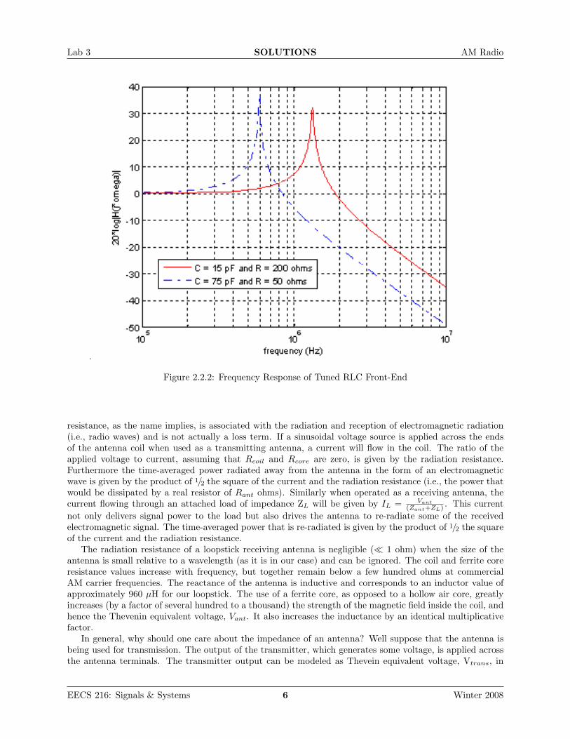
∣∣∣ dB has been computed and isplotted in Fig. 2.2.2 for two different RLC combinations, i.e., Rant = 200 Ω, L = 960 µH, C = 15 pF andRant = 50 Ω, L = 960 µH, C = 75 pF. Note that this circuit acts as a bandpass filter whose center frequency



VantVout

+

−

C

Xant = jωL

A A ARant

r

rr b

b

Antenna equivalent circuit Tuning capacitor

Figure 2.2.1: Antenna/Front-end Tuned RLC Circuit (preamplifier and mixer not shown)

is determined by the value of the capacitor, which is tunable by the radio listener. The capacitor value ischosen by the listener so that the center frequency of the bandpass filter corresponds to the carrier frequencyof the desired AM station.

2.2.1 Antenna (or How to Efficiently Receive a Signal)

An antenna is a device that provides a means of transmitting or receiving radio waves, i.e., electromagneticsignals that propogate through free-space. Antennas are common components of almost every communicationdevice, from radios to cellphones to laptops. To completely understand the operation of antennas requires aknowledge of electromagnetic theory that most of you have not yet acquired. You will learn this material inEECS 230 and EECS 330. Fortunately, however, a knowledge of some elementary physics (Phys 240) andcircuit theory (EECS 215) suffices to understand the basic ideas. For those of you who already have takenEECS 230/330 and wish to learn more about antennas, a good introductory book is [1].

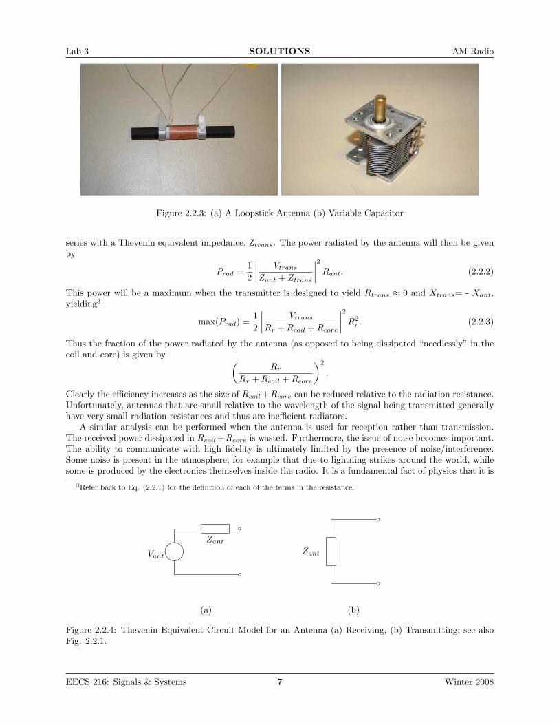
Antennas can take many different forms depending on the application. In your radio, the receivingantenna is a coil of wire wound around a ferrite core, i.e., an electrically non-conducting material withspecial magnetic properties. Such a coil depicted in Fig. 2.2.3(a) is known as a “loopstick” and is commonlyused for the antenna in AM radios.

The carrier wavelength, λc, is given by λc = c/fc, where c is the vacuum speed of light, 3x108 m/s, andfc is the carrier frequency in Hz, which for commercial AM lies between 540 KHz and 1700 KHz. Thus thecarrier wavelength is on the order of a few hundred meters. The electrical properties of an antenna can bemodeled by a Thevenin equivalent circuit consisting of a voltage source, Vant, in series with an impedance,Zant = Rant + jXant as shown in Fig. 2.2.4.

Zant is the same whether the antenna is transmitting or receiving a signal. Vant, on the other hand, is onlynon-zero when the antenna is receiving a signal. Time-varying electric and magnetic fields are associated withthe transmission of radio waves. According to Faraday’s Law of electromagnetics, a time-varying magneticfield radiated from a distant transmitter will induce an (open-loop) voltage drop, Vant, across the ends ofthe coil in a loopstick receiving antenna (in particular, the voltage induced across the ends of a loop ofwire equals the rate of change of flux through that loop). The voltage drop will be proportional to theproduct of the square-root of the power of the transmitted radio wave measured at the receiving antenna,the cross-sectional area of the coil, the number of turns in the coil and the relative permeability of the ferritecore.

Rant is the sum of three resistive terms (1) the radiation resistance Rr of the antenna, (2) the resistanceRcoil of the coil wire and (3) the magnetic losses (due to hysteresis) in the core Rcore,

Rant = Rr + Rcoil + Rcore. (2.2.1)

The coil wire and the core magnetic losses are parasitic effects, and with ideal materials (i.e., perfectlyconducting coil wires and ferrites without hysteresis), these resistive terms would be zero. The radiation



Figure 2.2.2: Frequency Response of Tuned RLC Front-End

resistance, as the name implies, is associated with the radiation and reception of electromagnetic radiation(i.e., radio waves) and is not actually a loss term. If a sinusoidal voltage source is applied across the endsof the antenna coil when used as a transmitting antenna, a current will flow in the coil. The ratio of theapplied voltage to current, assuming that Rcoil and Rcore are zero, is given by the radiation resistance.Furthermore the time-averaged power radiated away from the antenna in the form of an electromagneticwave is given by the product of 1/2 the square of the current and the radiation resistance (i.e., the power thatwould be dissipated by a real resistor of Rant ohms). Similarly when operated as a receiving antenna, thecurrent flowing through an attached load of impedance ZL will be given by IL = Vant

(Zant+ZL) . This currentnot only delivers signal power to the load but also drives the antenna to re-radiate some of the receivedelectromagnetic signal. The time-averaged power that is re-radiated is given by the product of 1/2 the squareof the current and the radiation resistance.

The radiation resistance of a loopstick receiving antenna is negligible ( 1 ohm) when the size of theantenna is small relative to a wavelength (as it is in our case) and can be ignored. The coil and ferrite coreresistance values increase with frequency, but together remain below a few hundred ohms at commercialAM carrier frequencies. The reactance of the antenna is inductive and corresponds to an inductor value ofapproximately 960 µH for our loopstick. The use of a ferrite core, as opposed to a hollow air core, greatlyincreases (by a factor of several hundred to a thousand) the strength of the magnetic field inside the coil, andhence the Thevenin equivalent voltage, Vant. It also increases the inductance by an identical multiplicativefactor.

In general, why should one care about the impedance of an antenna? Well suppose that the antenna isbeing used for transmission. The output of the transmitter, which generates some voltage, is applied acrossthe antenna terminals. The transmitter output can be modeled as Thevein equivalent voltage, Vtrans, in



Figure 2.2.3: (a) A Loopstick Antenna (b) Variable Capacitor

series with a Thevenin equivalent impedance, Ztrans. The power radiated by the antenna will then be givenby

Prad =12

∣∣∣∣ Vtrans

Zant + Ztrans

∣∣∣∣2 Rant. (2.2.2)

This power will be a maximum when the transmitter is designed to yield Rtrans ≈ 0 and Xtrans= - Xant,yielding3

max(Prad) =12

∣∣∣∣ Vtrans

Rr + Rcoil + Rcore

∣∣∣∣2 R2r . (2.2.3)

Thus the fraction of the power radiated by the antenna (as opposed to being dissipated “needlessly” in thecoil and core) is given by (

Rr

Rr + Rcoil + Rcore

)2

.

Clearly the efficiency increases as the size of Rcoil +Rcore can be reduced relative to the radiation resistance.Unfortunately, antennas that are small relative to the wavelength of the signal being transmitted generallyhave very small radiation resistances and thus are inefficient radiators.

A similar analysis can be performed when the antenna is used for reception rather than transmission.The received power dissipated in Rcoil +Rcore is wasted. Furthermore, the issue of noise becomes important.The ability to communicate with high fidelity is ultimately limited by the presence of noise/interference.Some noise is present in the atmosphere, for example that due to lightning strikes around the world, whilesome is produced by the electronics themselves inside the radio. It is a fundamental fact of physics that it is

3Refer back to Eq. (2.2.1) for the definition of each of the terms in the resistance.

Vant

Zant

bb

Zant

b

b

(a) (b)

Figure 2.2.4: Thevenin Equivalent Circuit Model for an Antenna (a) Receiving, (b) Transmitting; see alsoFig. 2.2.1.



impossible to completely remove the electronics noise because it is due to the thermal agitation of electronsin the circuit elements. In situations where the external atmospheric noise is negligible in comparison tothe signal level and the signal level is very weak, it is important to deliver as much of the received signal aspossible to the load in order to overcome the noise due to the radio electronics. We know that maximumpower delivery from the antenna to the load occurs when the impedance of the load is matched to that ofthe antenna. Let us assume for the moment that we have an antenna with very low parasitic resistance,Rcoil + Rcore, which is good from an efficiency point of view. In order to deliver maximum power fromthe antenna to the load under such conditions, the front-end receiver electronics must be designed to beimpedance matched, i.e., Zload = Z∗ant. For small (relative to the wavelength) antennas, however, this isvery difficult to achieve because Rr is very small.

In the AM radio band, atmospheric noise and interference are generally much larger than the electronicsnoise. Thus the fidelity is not limited by the electronics noise and therefore impedance matching of the loadto the antenna is not critical as long as a reasonable signal level is provided to the load.

2.2.2 RLC Resonant Circuit (or the First Step in Selecting a Station)

The variable capacitor indicated in Fig. 2.2.1 consists of two sets of interleaved parallel metallic plates asshown in Fig. 2.2.3 (b). One set of the plates can be rotated relative to the other, thus varying the overlapbetween the two plate sets, which in turn causes the capacitance to change. The capacitance ranges fromabout 10 pF when there is no overlap between the plates to 400 pF when the plates are fully overlapped.

The loopstick antenna together with the capacitor shown in Fig. 2.2.1 is a series RLC resonance circuit.Since this type of circuit and resonance phenomena in general play such an important role in electricalengineering, we will digress briefly to discuss these topics in some further detail below. You should be ableto derive for yourself Eqs. (2.2.4)-(2.2.7) below using the material that you learned in EECS 215.

The current flowing in the RLC circuit will be a maximum when the series RLC impedance is minimum.This impedance minimum occurs at a frequency for which the reactance of the inductor (i.e., jωL) exactlycancels the reactance of the capacitor (i.e., −j/ωC). When this condition occurs, the circuit is said to be atresonance. The resonance frequency is given by

fres =12π

1√LC

Hz or ωres =1√LC

rad/s (2.2.4)

and at the resonance frequency, the current achieves its peak value of Vant/Rant. The magnitude of thecurrent decreases monotonically as one moves away from resonance. The current drops to 1/

√2 of its peak

value when the source frequency is given by

f =12π

√1

LC+(

R

2L

)2

± 12π

R

2LHz (2.2.5)

Thus the 3 dB bandwidth, BW3dB , of the resonant response is equal to

BW3dB =12π

R

LHz (2.2.6)

While the resonance frequency does not lie exactly at the midpoint between the two 3 dB points, it is verynearly centered when BW3dB fres.

The ratio fres/BW3dB measures the “sharpness” of the resonance and is known as the quality factor, orQ of the circuit. Using Eqs. (2.2.4) - (2.2.6), it is easily shown that

Q = 2πfresL

R(2.2.7)

A high Q corresponds to a very sharp resonance, i.e, BW3dB fres. Note that the Q is inverselyproportional to R, which is the source of power dissipation in the resonator. Consequently Q increases asthe resonator losses decrease. The combination of the loopstick antenna and variable capacitor act as atunable bandpass filter as we saw in Fig. 2.2.2. Placing the resonance peak at the carrier frequency of thedesired radio station is the first step in receiving a signal and rejecting unwanted signals.



Continuing with our discussion of the radio front-end, the inductance of the loopstick antenna has beenmeasured to be approximately 960 µH while the variable capacitor has a range of about 10 pF to 400 pF.The bandwidth of the front-end resonant circuit is given by Eq. (2.2.6). Thus in order to estimate thebandwidth, we need to know the value of Rant, which as we indicated earlier is determined primarily by theloopstick coil resistance and the losses in the ferrite core. By replacing the voltage source, Vant, shown in Fig.2.2.1 by a function generator and measuring the resonant 3 dB bandwidth for different capacitance values,one can determine Rant as a function of the resonance frequency. As noted earlier, the value of Rant willincrease with frequency, and thus the Q of the filter will decrease, i.e., the filter will become less frequencyselective, as the resonance frequency increases.

You have also seen in lecture that the time-domain and frequency-domain descriptions of LTI systems arerelated via the Fourier transform. Namely the time response of an LTI system is given by the convolutionof the input with the system’s impulse response, and the frequency response is the product of the Fouriertransform of the input and the frequency response function. In addition, the frequency response functionis equal to the Fourier transform of the impulse response. Finally, the impulse response is equal to thederivative of the step response.

If we consider the series RLC circuit shown in Fig. 2.2.1, it is easy to verify that Vant and Vout are relatedby the following differential equation by noting that the sum of the voltage drops around the loop must bezero

LCd2Vout

dt2+ RC

dVout

dt+ Vout = Vant (2.2.8)

(In order to derive Eq. (2.2.8), you also need to recall that the instantaneous current flowing through acapacitor is given by C dv

dt and the instantaneous voltage drop across an inductor by L didt .) If we set the

Vant to be a unit step function, then the solution of Eq. (2.2.8) is given by (you will learn how to find thissolution later in the course using Laplace transform techniques)

Vout(t) = [1− (sinφ)−1e−(R/2L)t sin(ω t + φ)]u(t) (2.2.9)

where

ω =√

ω2res − (R/2L)2 rad/s (2.2.10)

φ = tan−1

(√ω2

res − (R/2L)2

(−R/2L)

)(2.2.11)

ωres =1√LC

rad/s (2.2.12)

Observe that the step response has an exponentially decaying sinusoidal component. When the Q is high,the oscillating frequency will be approximately equal to the resonance frequency, ωres, while the resonantbandwidth (see Eq. (2.2.6)) is related to the exponential decay rate, R/2L. These observations can be usedto determine the resonance frequency and the bandwidth experimentally.

2.3 First Stage of Demodulation: The Amplifier & Mixer in the Front-end

The output of the circuit shown in Fig. 2.2.1 is fed into a single field-effect transistor (FET) amplifier toboost the signal strength to a level suitable for the mixer to operate. The output of this amplifier feeds oneof the two mixer inputs. The mixer is a nonlinear device that produces at its output the product of thevoltages appearing at its two input ports (designated signal port and LO port). The local oscillator (LO)input is a sinusoid whose frequency is varied to select the channel (i.e., 540 KHz through 1700 KHz) to whichone wishes to listen. For our radio, the LO is the signal generator on your lab bench. Thus for a transmittedAM signal

x(t) = (A + bs(t)) cos(ωct + φ) (2.3.1)

the output of the mixer will be given by

(A + bs(t)) cos(ωct + φ) cos(ωLOt + θ) (2.3.2)



where θ−φ is the relative phase difference between the carrier and the LO. The receiver has no way of knowingthe value of this phase difference. A little bit of trigonometry (i.e., cos(x) cos(y) = 1

2 cos(x+y)+ 12 cos(x−y))

indicates that

(A + bs(t)) cos(ωct + φ) cos(ωLOt + θ) =12(A + bs(t)) cos((ωc + ωLO)t + φ + θ)

+12(A + bs(t)) cos((ωc − ωLO)t + φ− θ) (2.3.3)

Note that mixing has both translated the carrier frequency of the original signal up to a frequency of ωc+ωLO

and down to a frequency ωc−ωLO, as guaranteed by the following Fourier transform property: x(t) ↔ X(jω)implies that

x(t) cos(ωo t) ↔ 12X(j(ω + ωo)) +

12X(j(ω − ωo)). (2.3.4)

A frequency domain representation of the operation of the modulator and mixer is illustrated in Fig. 2.3.1.

ω-

6

?

@@

6

(a) Original Baseband Signal SpectrumA + bs(t) ↔ 2πAδ(ω) + bS(jω)

ω-ωc ωc

66

-

6

?

@@

@@

(b) AM Signal Spectrumx(t) = (A + bs(t)) cos(ωct) ↔ X(jω)

X(jω) = Aπδ(ω − ωc) + 12bS(j(ω − ωc)) + Aπδ(ω + ωc) + 1

2bS(j(ω + ωc))

ω-ωc − ωLO ωc + ωLOωc − ωLO -ωc + ωLO

66 66

-

6

?

@@

@@

@@

@@

(c) Signal Spectrum After Mixing with LO (drawn for the case where ωLO > ωc )

Figure 2.3.1: Signal Spectrum (a) original signal, (b) signal at transmitter after AM modulation, (c) signalat the output of the radio front-end mixer.

For simplicity of illustration,we have assumed that the spectrum of s(t) is purely real, has a triangularshape4, and that θ = φ = 0.

4You should know a time-domain signal whose Fourier transform has these properties.



Notes:

1. The figures are not drawn to scale.

2. The spectrum, S(jω), of the original baseband signal (e.g., music or voice), s(t), is generally complex-valued, having a magnitude and phase. For simplicity of illustration, we have chosen a spectrumthat is real-valued. An actual spectrum would look quite different. Note that for commercial AM|S(jω)| ≈ 0 for |ω| > 2π(5000) rad/s.

3. In part (b) of Fig. 2.3.1, the phase, φ, of the carrier has been assumed to be zero. In general, thisphase will be non-zero. The introduction of a non-zero phase will not affect the position or the shapeof the spectrum shown in Fig. 2.3.1 (b). Note that it will simply cause the spectrum to be multipliedby a scale factor of either e±jφ by recalling that

cos(ωLOt + φ) =12ejφejωLOt +

12e−jφe−jωLOt (2.3.5)

A similar comment is applicable to Fig. 2.3.1 (c) and the phase, θ, of the LO.

2.4 IF Filter or How to Practically Select a Station and Demodulate a Signal

The intermediate frequency (IF) filter shown in Fig. 2.1.1 is a bandpass filter centered at fIF (the IFfrequency). In the ideal case, the frequency response function of this filter would be that shown in Fig. 2.4.1below. Observe (see Fig. 2.3.1 (c)) that by choosing the LO frequency appropriately we can use the mixer

HIF (j2πf)

ffIF−fIF

-

6

?

10 KHz 10 KHz- -

Figure 2.4.1: Ideal IF Filter

to shift the frequency of the modulated signal so that the modulated signal passes through the IF filterundistorted (assuming, of course, that the bandwidth of the IF filter exceeds the bandwidth of the messagesignal). Either of two frequency choices are possible for the LO, namely (assuming fc > fIF )

ωIF = ωc − ωLO → fLO = fc − fIF (2.4.1)

orωIF = −ωc + ωLO → fLO = fc + fIF (2.4.2)

as indicated below in Fig. 2.4.2 and 2.4.3, respectively.In either case the output of the IF filter (up to a multiplicative constant) becomes

(A + bs(t)) cos(ωIF t + φ− θ).

Thus, if the output of the IF filter is fed into a properly designed envelope detector (see Lab 2), the outputof the envelope detector will be A + bs(t) (up to a multiplicative constant). Finally the constant term, A,can be removed by placing a capacitor in series with the output of the envelope detector (see Fig. 2.1.1) toblock the DC component, leaving just the information signal s(t) (up to a multiplicative constant). Thusour radio will have recovered the transmitted information signal, s(t)! A similar result is obtained whenfc < fIF .



fLO = fc − fIFfLO = fc − fIF fLO = fc − fIF

ffIF−fIF fc−fc fLO + fc = 2fc − fIF−fLO − fc = −2fc + fIF

-

6

?

@@

@@

6 66 6

RR

Figure 2.4.2: Using LO to Mix into IF Band when fLO = fc − fIF

fLO = fIF + fc

fLO = fIF + fc

fLO = fIF + fcfLO = fIF + fc

ffIF−fIF fc−fc fLO + fc = 2fc + fIF−fLO − fc = −2fc − fIF

-

6

?

@@

@@

6 66 6

j R

Y

Figure 2.4.3: Using LO to Mix into IF Band when fLO = fIF + fc

2.5 A Simple Butterworth Filter Realization of the IF Filter

We have seen that the IF filter should be a bandpass filter. Bandpass filters can take many differentforms. For example, a bandpass Butterworth filter of order N is characterized by the following (magnitude)frequency response function

|H(jω)|2 =Ho

1 + [2(ω − ωo)/β]2N, (2.5.1)

where the center frequency of the filter is ωo rad/s, the peak gain is Ho and the 3-dB bandwidth is βrad/s. This filter approaches an ideal bandpass filter as N gets large, since for N large, the frequencyresponse function is nearly constant and equal to Ho over the passband, |ω−ωo| < β, and decreases rapidlytowards zero as one moves outside of the passband. Note that the 3-dB bandwidth alone does not indicatethe sharpness of the transition from passband to stop band. For the Butterworth filter, both the 3-dBbandwidth and the filter order N determine the filter performance.

In this lab, we will construct a very simple, op amp-based, IF filter. This filter does not have a particularlysharp passband-to-stopband transition, but it is relatively simple to build and will be sufficient for ourapplication.

The frequency response function of our bandpass filter is given by

H(s) = Hoβs

s2 + βs + ω2o

(2.5.2)

where s = jω. Note that Eq. (2.5.2) can be rewritten as

H(jω) = Hoβjωo

(ωo + ω)(ωo − ω) + jβω= Ho

1ωωo

+ j (ω−ωo)βωo/(ωo+ω)

(2.5.3)



For ω in the vicinity of ωo, Eq. (2.5.3) reduces to

H(jω) ≈ Ho1

ωo

ωo+ j (ω−ωo)

βωo/(ωo+ωo)

= Ho1

1 + j (ω−ωo)β/2

. (2.5.4)

It follows that the frequency response function in Eq. (2.5.4) achieves a maximum value of Ho at a frequencyof ωo rad/s with a 3-dB bandwidth equal to β rad/s. Moreover, this result applies to our original frequencyresponse function as long as β +ωo ≈ ωo, that is, when β is a small fraction of ωo, which one typically writesas β ωo.

The bottom line is that the bandpass filter in Eq. (2.5.3) achieves a maximum value of Ho at a frequencyof ωo rad/s with an approximate 3-dB bandwidth of

BW3dB ≈ β vaild when β ωo. (2.5.5)

Image Frequencies: This discussion is carried out for the case that the carrier frequency is greater thanthe center frequency of the IF filter. Analyzing the other case is left to the reader.

By examining Fig. 2.4.3, one can see that when the LO frequency fLO is set equal to fc + fIF , not onlydoes the signal centered at fc get mixed into the IF band, but so does any signal centered at

fimag = fIF + fLO = fc + 2fIF . (2.5.6)

The frequency band centered at fimag is known as the image band. Using Eq. (2.5.6), we conclude that

fimag − fc = 2fIF (valid when fLO = fc + fIF & fc > fIF ). (2.5.7)

Thus the separation between the carrier frequency of the desired station (i.e., the one you wish to receive)and the center frequency of the image band (which also ends up in the passband of the IF filter after themixer) is equal to twice the IF frequency.

A similar result is obtained when the situation illustrated in Fig. 2.4.2 is considered. Specifically, whenfLO = fc − fIF ,

fimag = |fIf − fLO| = |2fIF − fc|. (2.5.8)

Then the separation between the carrier frequency of the desired station (i.e., the one you wish to receive)and the center frequency of the image band is equal to

fc − fimag =

2fIF , fc > 2fIF

2(fc − fIF ), fc < 2fIF

(valid when fLO = fc − fIF & fc > fIF ). (2.5.9)

We conclude that when the LO frequency is chosen to be the higher of the two possible choices, namelyfc + fIF , then the IF filter cannot separate two AM stations whose carrier frequencies differ by twice theIF frequency, and according to Eq. (2.5.9), the separation between the desired and image stations may beeven less when the lower LO frequency is used5. In either case, the RLC front-end (recall the antenna andresonance tuning circuit) must sufficiently attenuate signals in the image band when tuned to the carrierfrequency of the desired station; otherwise, the image band will corrupt the demodulation of the desiredstation. Consequently, the higher LO frequency is often chosen in order to simplify6 the design of the RLCfilter in the front-end. AM radios are designed so that both the LO frequency and the resonance frequencyof the RLC front-end are set together when a station is selected. The capacitor in the front-end RLC circuitis adjusted so that the resonance frequency of this circuit is equal to the carrier frequency, fc, of the stationthat is to be received, while the LO frequency is set to one of the two frequencies |fc ± fIF |.

5When the lower LO frequency fLO = fc − fIF is used and fc < 2fIF , then the separation of the carrier and imagefrequencies is 2(fc − fIF ) < 2fIF , which is smaller than the separation of the carrier and image frequencies achieved with thehigher LO frequency fLO = fc + fIF . When fc > 2fIF , both LO frequencies give the same separation.

6The smaller the distance between the carrier and image frequencies becomes, the narrower the bandwidth must be in theRLC filter in order to attenuate the image band.



The frequency selectivity (i.e., its Q) of a bandpass filter is a measure of its ability to attenuate signalsthat do not lie near the center frequency of its passband, i.e., within a small fraction of the center frequencyof the passband. Consequently if the IF frequency is properly chosen, then the front-end RLC circuit doesnot need to have much frequency selectivity in order to reject the image frequency because fc−fimag

fc= 2 fIF

fc

when fLO = fc + fIF . For example, if fIF = 455 KHz, which is a common choice in commercial radios, thenthe desired and image frequencies are separated by 910 KHz and the front-end series RLC filter does notrequire much frequency selectivity. The IF filter for the radio that you will build in this lab will be centeredat approximately 100 KHz.

2.6 Why a Superheterodyne Receiver?

A radio, like the one built in this lab experiment, which has an IF filter with a fixed center frequency and avariable frequency LO (that can be used to shift the desired station into the IF band by mixing), is knownas a superheterodyne receiver. As mentioned earlier, the superheterodyne receiver was invented by EdwinArmstrong in 1920 and is still widely used today.

It is natural to ask why we shouldn’t eliminate the LO, the mixer, and the fixed IF filter and replace theseelements by a single bandpass filter with a tunable center frequency. While such an approach is possible inprinciple, it is difficult in practice to build tunable bandpass filters that have adequate frequency selectivityand gain.

Perhaps an even better approach, then, would be to mix the frequency of the desired station down tobaseband (i.e., choose fLO = fc) and then simply low pass filter the output of the mixer. This approach,however, may lead to a very weak signal, and one that will experience power fluctuations as the followinganalysis indicates.

Consider the signal at the output of the mixer:

(A + bs(t)) cos(ωct + φ) cos(ωLOt + θ)

=12(A + bs(t)) cos((ωc + ωLO)t + θ + φ) +

12(A + bs(t)) cos((ωc − ωLO)t + φ− θ) (2.6.1)

When fLO = fc, this signal becomes

(A + bs(t)) cos(ωct + φ) cos(ωct + θ) =12(A + bs(t)) cos(2ωct + φ + θ) +

12(A + bs(t)) cos(φ− θ) (2.6.2)

The term at twice the carrier frequency will be strongly attenuated by the low-pass filter, leaving 12 (A +

bs(t)) cos(φ − θ) at the output7. Note that for many values of φ − θ, for example, φ − θ ≈ π/2, thedemodulated signal will be greatly diminished in strength. Indeed, for the case φ − θ = π/2, the signalstrength is identically zero! It follows that when | cos(φ − θ)| ≈ 0, the presence of noise will significantlydegrade the quality of reception. Furthermore, the relative phase difference between the carrier and the LOwould vary when the distance between the transmitter and the receiver changes, as in a moving car. Thus,if the radio is moving, the demodulated signal strength will be time-varying (the radio would fade in andout). Although radios can be built to track the relative phase and make LO adjustments to keep the relativephase small (a method known as coherent reception), such radios are more expensive.

The use of envelope detection obviates the need to track the relative phase. There is, however, a price tobe paid for this simplicity. Envelope detection requires that a DC bias, A, be added to the signal beforemodulation. This DC bias is chosen to ensure that the quantity A+ bs(t) always remains positive, otherwisethe message signal s(t) cannot be uniquely recovered from the envelope, |A+ bs(t)|. The presence of the DCbias term means that the transmitter must use additional power, since it needs to transmit both the signaland the DC bias term. Because there are many fewer transmitters than receivers, it was decided in the earlydays that it was better to burden the transmitter rather than the receiver with the extra cost. Given thelow cost and advanced state of electronics today, such a trade-off may no longer be favorable.

7Note that the constant term A can be removed by a DC blocking capacitor; see Fig. 2.1.1.



3 Pre-lab Assignment

3.1

(a) Consider the RLC circuit shown in Fig. 2.2.1. Compute the frequency response function Vout(jω)Vant(jω) .

Your answer should be of the following form

H(jω) =Vout(jω)Vant(jω)

=1

a1s2 + a2s + 1(3.1.1)

where s ≡ jω.

(b) Assuming R = 20 Ω, L = 960µH and C = 100 pF, compute and plot (use Matlab) the quantity20 log10 |H(jω)|, where H(jω) is given by Eq. (3.1.1), over the frequency range 100 KHz to 10 MHz.Repeat for R = 90Ω, L = 960µH and C = 30 pF.

For your plots use the logspace command, freq = logspace(5, 7, 10000), to specify the frequencypoints at which the frequency response function is to be computed8. Plotting should be done usingthe semilogx and grid Matlab commands as was done to generate Fig. 2.2.2. Both plots shouldappear on a single graph with appropriate legends and axis titles. On your plot, specify the frequencyat the peak, the 3-dB bandwidth BW3dB and quality factor Q for each of the two series RLC circuits.Compare your results with the values computed using Eqs. (2.2.4) and (2.2.6). When you’re donewith this problem, you should present all of your information in two tables as in Table 3.1 below, withone table containing values read off from the plot and the other containing values computed from theequations.

Peak freq. (kHz) 3dB BW (kHz) Quality FactorC = 100 pFC = 30 pF

Table 3.1: Values from Plot or Equations

SOLUTION:(a):

Vout(jω)Vant(jω)

=ZC

Zant + ZC(3.1.2)

H(jω) =Vout(jω)Vout(jω)

= ZRLC =1/sC

Rant + sL + 1/sC(3.1.3)

H(jω) =1

LCs2 + RCs + 1(3.1.4)

(b): From the plot below, the frequency at the peak, the bandwidth and the Q are:

Peak freq. (kHz) 3dB BW (kHz) Quality FactorC = 100 pF 513.7 3.3 155.7C = 30 pF 937.8 14.9 62.9

Table 3.2: Values from Plot (Fig. 3.1). When finding the 3dB BW from the plot, recall that the y-axis is inunits of dB.

From Eqs. (2.2.4) and (2.2.6), the frequency at the peak and the bandwidth are:



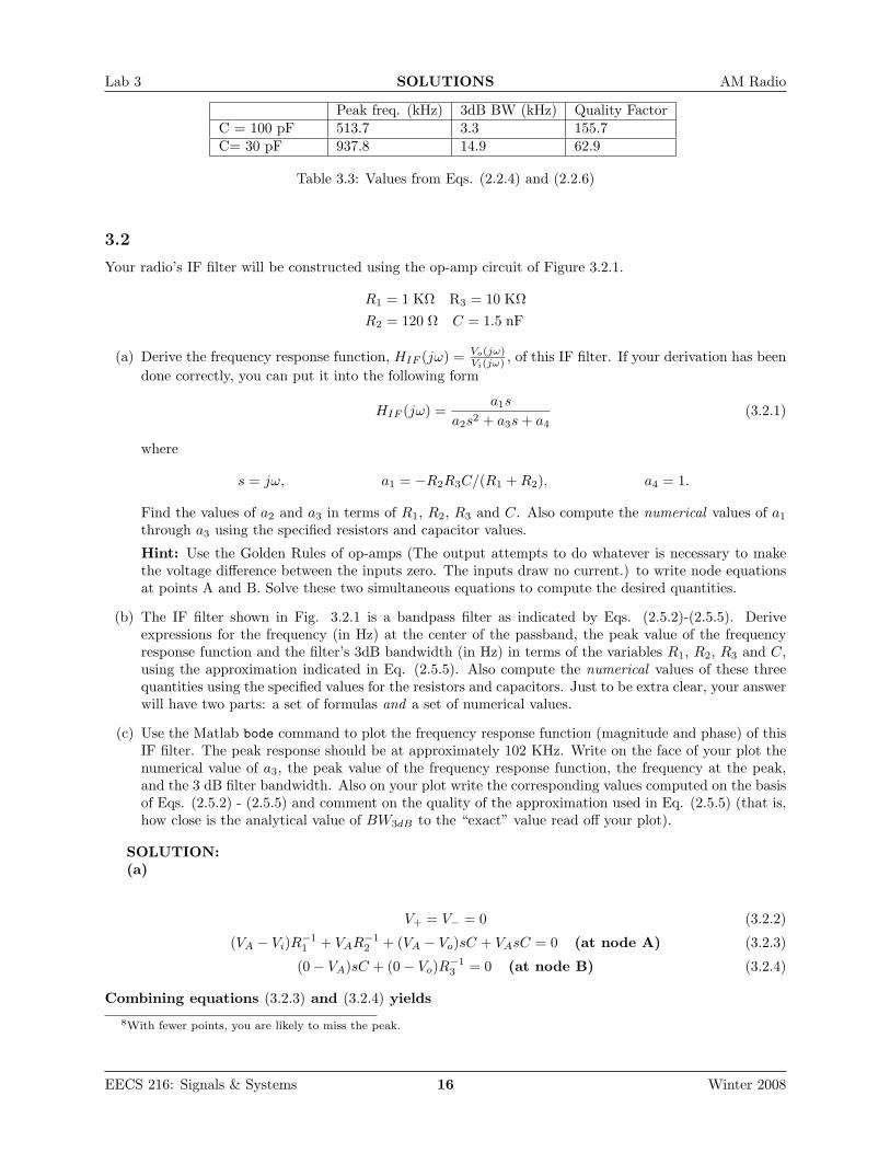
Peak freq. (kHz) 3dB BW (kHz) Quality FactorC = 100 pF 513.7 3.3 155.7C= 30 pF 937.8 14.9 62.9

Table 3.3: Values from Eqs. (2.2.4) and (2.2.6)

3.2

Your radio’s IF filter will be constructed using the op-amp circuit of Figure 3.2.1.

R1 = 1 KΩ R3 = 10 KΩR2 = 120 Ω C = 1.5 nF

(a) Derive the frequency response function, HIF (jω) = Vo(jω)Vi(jω) , of this IF filter. If your derivation has been

done correctly, you can put it into the following form

HIF (jω) =a1s

a2s2 + a3s + a4(3.2.1)

where

s = jω, a1 = −R2R3C/(R1 + R2), a4 = 1.

Find the values of a2 and a3 in terms of R1, R2, R3 and C. Also compute the numerical values of a1

through a3 using the specified resistors and capacitor values.

Hint: Use the Golden Rules of op-amps (The output attempts to do whatever is necessary to makethe voltage difference between the inputs zero. The inputs draw no current.) to write node equationsat points A and B. Solve these two simultaneous equations to compute the desired quantities.

(b) The IF filter shown in Fig. 3.2.1 is a bandpass filter as indicated by Eqs. (2.5.2)-(2.5.5). Deriveexpressions for the frequency (in Hz) at the center of the passband, the peak value of the frequencyresponse function and the filter’s 3dB bandwidth (in Hz) in terms of the variables R1, R2, R3 and C,using the approximation indicated in Eq. (2.5.5). Also compute the numerical values of these threequantities using the specified values for the resistors and capacitors. Just to be extra clear, your answerwill have two parts: a set of formulas and a set of numerical values.

(c) Use the Matlab bode command to plot the frequency response function (magnitude and phase) of thisIF filter. The peak response should be at approximately 102 KHz. Write on the face of your plot thenumerical value of a3, the peak value of the frequency response function, the frequency at the peak,and the 3 dB filter bandwidth. Also on your plot write the corresponding values computed on the basisof Eqs. (2.5.2) - (2.5.5) and comment on the quality of the approximation used in Eq. (2.5.5) (that is,how close is the analytical value of BW3dB to the “exact” value read off your plot).

SOLUTION:(a)

V+ = V− = 0 (3.2.2)

(VA − Vi)R−11 + VAR−1

2 + (VA − Vo)sC + VAsC = 0 (at node A) (3.2.3)

(0− VA)sC + (0− Vo)R−13 = 0 (at node B) (3.2.4)

Combining equations (3.2.3) and (3.2.4) yields

8With fewer points, you are likely to miss the peak.



H(jω) =a1s

a2s2 + a3s + a4=

−[R2R3C/(R1 + R2)]sR1R2

R1+R2R3C2s2 + 2 R1R2

R1+R2Cs + 1

(3.2.5)

and therefore

a1 = −[R2R3C/(R1 + R2)]

a2 =R1R2

R1 + R2R3C

2

a3 = 2R1R2

R1 + R2C

a4 = 1

With C = 1.5 nF, R1 = 1KΩ, R2 = 120Ω, R3 = 10KΩ, Eq. (3.2.5) becomes

H(jω) =−1.61× 10−6s

2.41× 10−12s2 + 3.21× 10−7s + 1(3.2.6)

where s = jω.Thus

a1 = −1.61x10−6,

a2 = 2.41x10−12,

a3 = 3.21x10−7,

a4 = 1.

(b):We can re-write Eq. (3.2.5) as

H(jω) =(a1/a2)s

s2 + (a3/a2)s + a4/a2=

−1R1C s

s2 + 2R3C s + R1+R2

R1R2R3C2

(3.2.7)

and comparing Eq. (3.2.7) to Eq. (2.5.2), we find

ωo =√

a4

a2=√

R1 + R2

R1R2R3C2rad/s (3.2.8)

β =a3

a2=

2R3C

rad/s (3.2.9)

H0 =a1

a3=−R3

2R1(3.2.10)

Therefore

ωo = 6.44× 105 rad/s = 102.5 KHz (center frequency),

β = 1.33× 105 rad/s = 21.2 KHz (3 dB bandwidth),

|Ho| = 5 = 13.98 dB (gain at center of band).

(c):From the plot, we conclude ωo= 6.5x105 rad/s= 103 KHz (center frequency), β=1.3x105

rad/s=21 KHz (3 dB bandwidth), Ho=5=13.98 dB (gain at center of band). The approxima-tion is seen to be excellent!



3.3

Assume that you wish to receive a radio station operating at a carrier frequency of 1600 KHz and the IFfilter is centered at 100 KHz.

a) Find the two possible choices for the LO frequency. For each of these cases indicate the center frequencylocation of the image band.

b) Repeat for the case when the carrier frequency is at 530 KHz.

Once you have calculated the values in a) and b), write them in a table like Table 3.2.

fc (KHz) fLO1 (KHz) fLO2 (KHz) fimage1 (KHz) fimage2 (KHz)1600530

Table 3.4: Required LO frequencies and Corresponding Image Frequencies

SOLUTION:(a):

fLO1 = fc4− fIF = 1600KHz− 100 KHz = 1500 KHzfimage1 = fc − 2fIF = 1400KHz

fLO2 = fc + fIF = 1600KHz + 100KHz = 1700 KHzfimage2 = fc + 2fIF = 1800KHz

(b):

fLO1 = fc − fIF = 530KHz− 100KHz = 430KHzfimage1 = fc − 2fIF = 330KHz

fLO2 = fc + fIF = 530KHz + 100KHz = 630 KHzfimage2 = fc + 2fIF = 730KHz

Thus, assuming fLO1 < fLO2,

fc (KHz) fLO1 (KHz) fLO2 (KHz) fimage1 (KHz) fimage2 (KHz)1600 1500 1700 1400 1800530 430 630 330 730

Table 3.5: Required LO frequencies and Corresponding Image Frequencies

3.4

Sketch the equivalents of Figs. 2.4.2 and 2.4.3 for the case that 12fIF < fc < fIF ; recall that Figs. 2.4.2 and

2.4.3 assumed that fc > fIF . You will have two sketches, one for the case fLO = fIF − fc and another forthe case fLO = fIF + fc.

SOLUTION:Sketches given below in Figs. 3.4.1, 3.4.2:



3.5 This problem is optional (i.e., not required, and worth zero points, even ifcompleted). No hints will be given in office hours. The result here doesNOT apply to the mixer we will use in the lab. It is a very hard test ofyour knowledge of the Fourier transform applied to modulation.

Consider the AM radio block diagram shown below in Fig. 3.5.1. The “special” mixer performs the operationindicated in Fig. 3.5.2.

The filter shown has |H(jω)| = 1, and therefore it passes all frequency components without altering theirmagnitudes. Any filter whose frequency response function satisfies the condition |H(jω)| = c, where c is aconstant independent of frequency is known as an all-pass filter. The phase response chosen for the filtershown in Fig. 3.5.2 is

∠H(jω) =

π2 , ω > 0

−π2 , ω < 0

(3.5.1)

(a) Suppose that the input, x(t), shown in Fig. 3.5.2 consists of the desired radio station at a carrierfrequency of ωc plus a second station centered at the image frequency, ωimag = ωc + 2ωIF where theLO frequency is given by ωLO = ωc + ωIF . Thus we can write

x(t) = [A1 + b1s1(t)] cos(ωct) + [A2 + b2s2(t)] cos(ωimagt). (3.5.2)

Derive expressions for I(jω), Q(jω), W (jω) and Y (jω) in terms of A1, b1, A2, b2, S1(jω) and S2(jω)for frequencies that lie inside the IF filter band. Also find an expression for the output of the IF filteras a function of time when the IF input is y(t).

(b) Consider the AM Radio block diagram shown in Fig. 3.5.1 and 3.5.2. The antenna that appears inFig. 3.5.1 consists of a loopstick. The front-end does not contain a resonant series RLC circuit forimage rejection. Does this radio have an image problem? Explain you answer.

Suggest an appropriate name for the “special” mixer shown in Fig. 3.5.2.

SOLUTION:

(a): I:

I(jω) = A1πδ(ω − ωIF ) + A1πδ(ω + ωIF ) +12b1[S1(j(ω − ωIF )) + S1(j(ω + ωIF ))]

+ A2πδ(ω − ωIF ) + A2πδ(ω + ωIF ) +12b2[S2(j(ω − ωIF )) + S2(j(ω + ωIF ))]

Q:

Q(jω) =A1π

jδ(ω − ωIF )− A1π

jδ(ω + ωIF ) +

12j

b1[S1(j(ω − ωIF ))− S1(j(ω + ωIF ))]

− A2π

jδ(ω − ωIF ) +

A2π

jδ(ω + ωIF )− 1

2jb2[S2(j(ω − ωIF ))− S2(j(ω + ωIF ))]

W:

W (jω) = jA1π

jδ(ω − ωIF )− (−j)

A1π

jδ(ω + ωIF ) +

12j

b1[(j)S1(j(ω − ωIF ))− (−j)S1(j(ω + ωIF ))]

− (j)A2π

jδ(ω − ωIF ) + (−j)

A2π

jδ(ω + ωIF )− 1

2jb2[(j)S2(j(ω − ωIF ))− (−j)S2(j(ω + ωIF ))]

Y:

Y (jω) = I(jω) + W (jω) = 2A1πδ(ω − ωIF ) + 2A1πδ(ω + ωIF )+ b1[S1(j(ω − ωIF ) + S1(j(ω + ωIF ))]



y(t) after IF filer:y(t) = 2(A1 + b1s1(t)) cos(ωIF t)

Note that the signal at the image frequency has been removed!

(b): From you result in part (a) it is obvious that this radio does not have an image problem.As you might expect, the “special” mixer is known as an image rejection mixer.



References

[1] Warren L. Stutzman and Gary A. Thiele. Antenna Theory and Design. John Wiley and Sons, secondedition, 1998.



Figure 3.1.1: Plot 20 log10 |H(jω)|

""

"

bb

b−+

LF356N

HHH

R3

A A AR1

HHH

R2

b+Vi

rBA

C

C

rr b+

V0

Figure 3.2.1: IF Filter



Figure 3.2.2: Frequency Response of IF Filter

fLO = fIF − fcfLO = fIF − fc fLO = fIF − fcfLO = fIF − fc

ffIF−fIF fc−fc fc − fLO = 2fc − fIF−fc + fLO = −2fc + fIF

-

6

?

@@ @@

6 66 6

RR

Figure 3.4.1: Using LO to Mix into IF Band (fLO = fIF − fc)



ffIF−fIF fc−fc fc + fLO = 2fc + fIF−fc − fLO = −2fc − fIF

-

6

?

@@ @@

6 66 6 j R

Figure 3.4.2: Using LO to Mix into IF Band (fLO = fIF + fc)



@

Antenna

Front-endAmplifier

“Special”

MixerIF Filter

EnvelopeDetector

Amplifer(Gain=5)

x(t) y(t)

DC blockingcapacitor

- - -

n&%'$Speaker

Figure 3.5.1: AM Radio With “Special” Mixer

x(t) +-

-

6

6

sin(ωLOt)

cos(ωLOt)

@@

@@

-

i(t)

q(t) w(t)

?

H(jω)

6

- y(t)

Figure 3.5.2: “Special” Mixer


eecs 216 winter 2008 solutions lab 3: am radio …...eecs 216 winter 2008 solutions lab 3: am radio...

Documents