ee 495 modern navigation systems noise & random processes mon, march 02 ee 495 modern navigation...

EE 495 Modern Navigation Systems

Noise & Random Processes

Mon, March 02 EE 495 Modern Navigation Systems Slide 1 of 19

http://www.erau.edu/


Mon, March 02 EE 495 Modern Navigation Systems

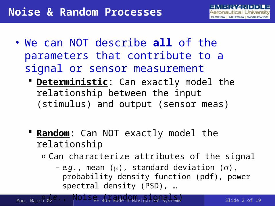
• We can NOT describe all of the parameters that contribute to a signal or sensor measurement Deterministic: Can exactly model the relationship between

the input (stimulus) and output (sensor meas)

Random: Can NOT exactly model the relationshipo Can characterize attributes of the signal

– e.g., mean (), standard deviation (), probability density function (pdf), power spectral density (PSD), …

o i.e., Noise (random signals)

Slide 2 of 19




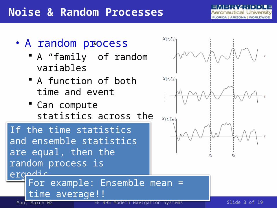
• A random process A “family” of random variables A function of both time and

event Can compute statistics across

the ensemble or across time

If the time statistics and ensemble statistics are equal, then the random process is ergodic.

For example: Ensemble mean = time average!!

Slide 3 of 19




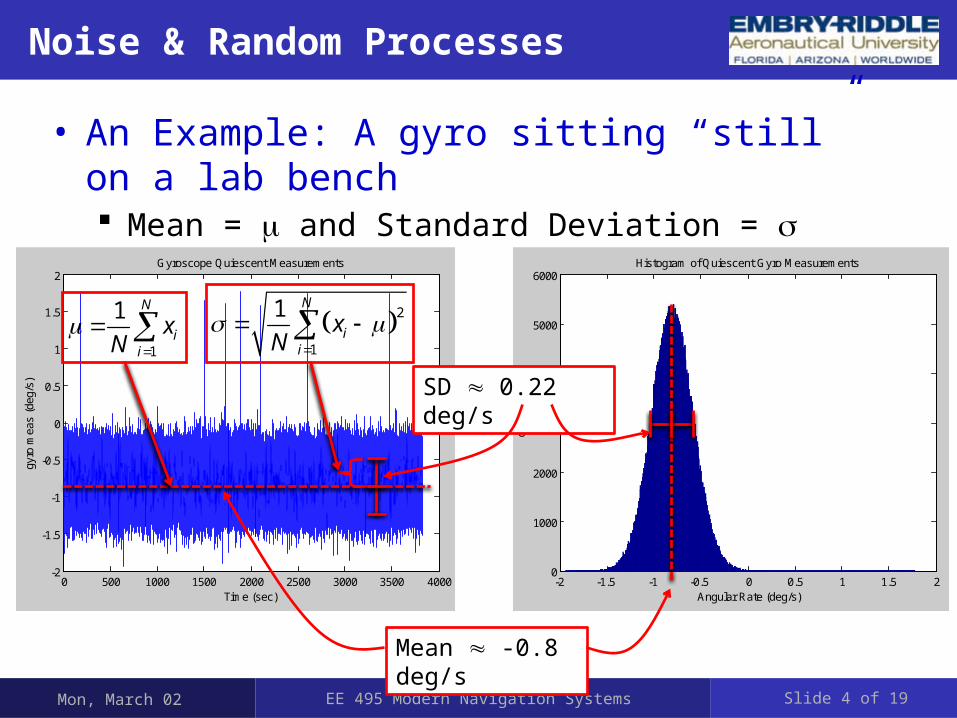
• An Example: A gyro sitting “still” on a lab bench Mean = and Standard Deviation =

0 500 1000 1500 2000 2500 3000 3500 4000-2

-1.5

-1

-0.5

0

0.5

1

1.5

2

gyro

mea

s (d

eg/s

)

Gyroscope Quiescent Measurements

Time (sec)

1

1 N

ii

xN

21

1 N

ii

xN

-2 -1.5 -1 -0.5 0 0.5 1 1.5 20

1000

2000

3000

4000

5000

6000

coun

t

Histogram of Quiescent Gyro Measurements

Angular Rate (deg/s)

Mean -0.8 deg/s

SD 0.22 deg/s

Slide 4 of 19




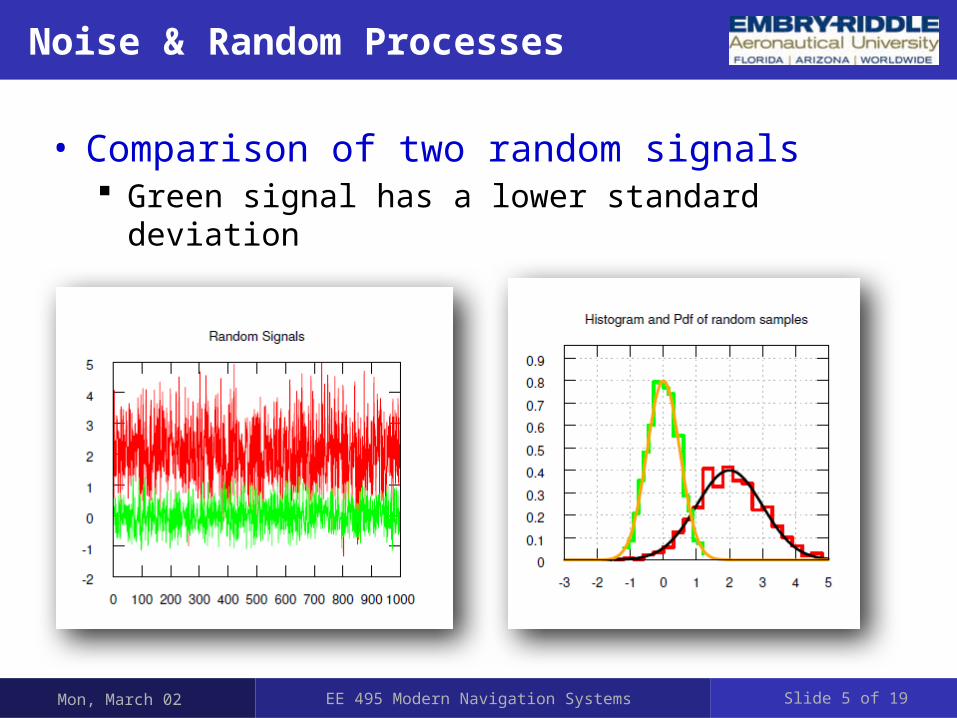
• Comparison of two random signals Green signal has a lower standard deviation

Slide 5 of 19




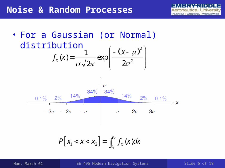
• For a Gaussian (or Normal) distribution

22

1( ) exp

22x

xf x

2

11 2 ( )

x

xxP x x x f x dx

Slide 6 of 19


0 0.1 0.2 0.3 0.4 0.5 0.6 0.7 0.8 0.9 1-0.01

0

0.01

0.02

0.03

0.04

0.05

Rxx

()

Autocorrelation Function of Quiescent Gyro Measurements

(sec)



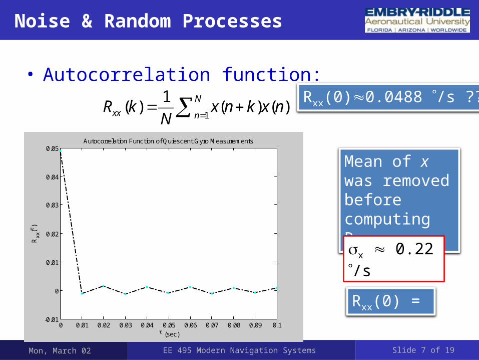
• Autocorrelation function:

1

1( ) ( ) ( )

N

xx nR k x n k x n

N

0 0.01 0.02 0.03 0.04 0.05 0.06 0.07 0.08 0.09 0.1-0.01

0

0.01

0.02

0.03

0.04

0.05

Rxx

()

Autocorrelation Function of Quiescent Gyro Measurements

(sec)

Rxx(0)0.0488 /s ??

Mean of x was removed before computing Rxx

Slide 7 of 19

x 0.22 /s

Rxx(0) =


0 0.1 0.2 0.3 0.4 0.5 0.6 0.7 0.8 0.9 1-9

-8

-7

-6

-5

-4

-3

-2

-1

0

1x 10

-3

Rxy

()

Crosscorrelation Function of Two Gyro Measurements

(sec)



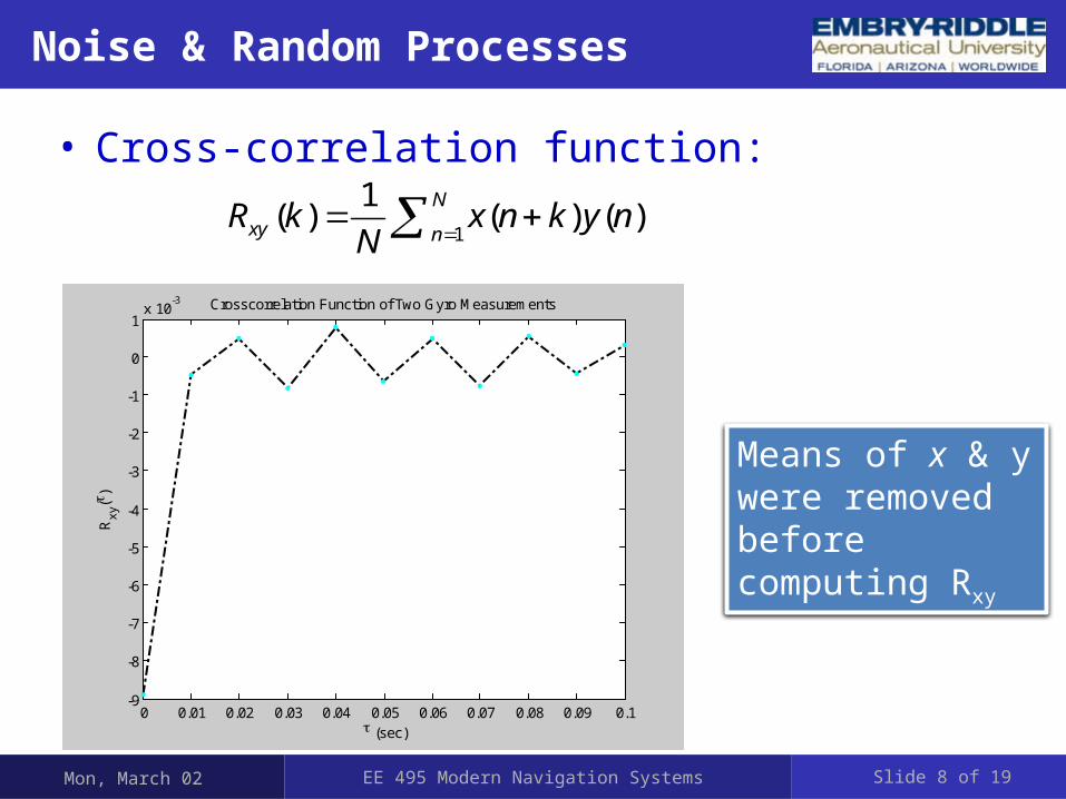
• Cross-correlation function:

1

1( ) ( ) ( )

N

xy nR k x n k y n

N

Means of x & y were removed before computing Rxy

0 0.01 0.02 0.03 0.04 0.05 0.06 0.07 0.08 0.09 0.1-9

-8

-7

-6

-5

-4

-3

-2

-1

0

1x 10

-3

Rxy

()

Crosscorrelation Function of Two Gyro Measurements

(sec)

Slide 8 of 19




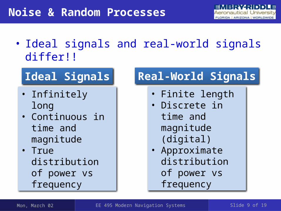
• Ideal signals and real-world signals differ!!

• Infinitely long• Continuous in time

and magnitude• True distribution of

power vs frequency

Ideal Signals• Finite length• Discrete in time and

magnitude (digital)• Approximate

distribution of power vs frequency

Real-World Signals

Slide 9 of 19


Noise & Random ProcessesEnergy Signals vs Power Signals


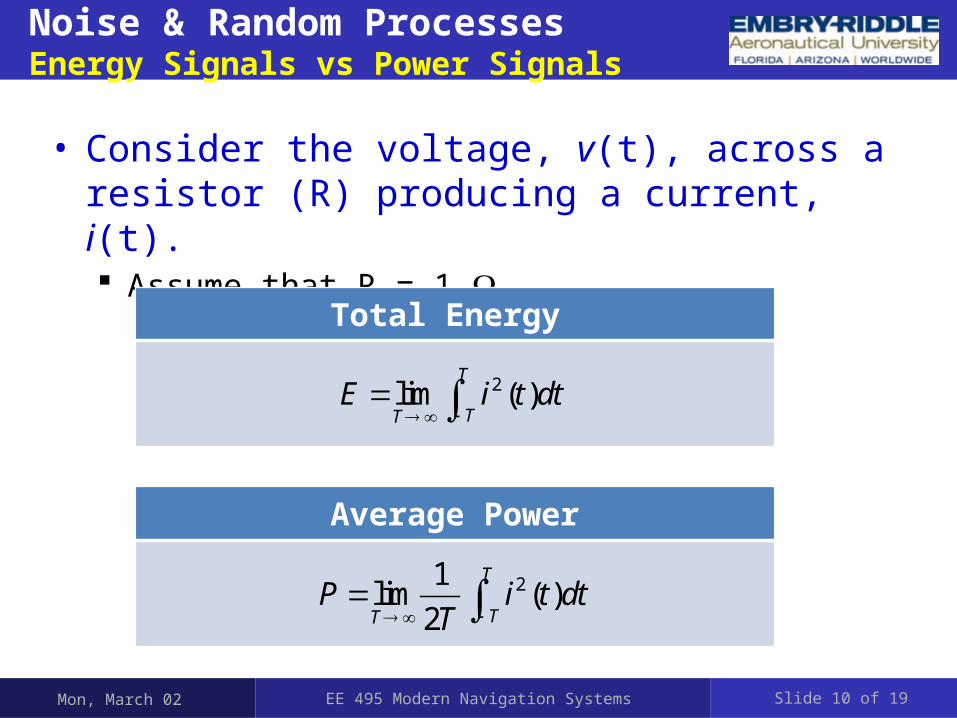
• Consider the voltage, v(t), across a resistor (R) producing a current, i(t). Assume that R = 1

Total Energy

2lim ( )T

TTE i t dt

Average Power

21lim ( )

2

T

TTP i t dt

T

Slide 10 of 19


Noise & Random ProcessesEnergy Signals vs Power Signals


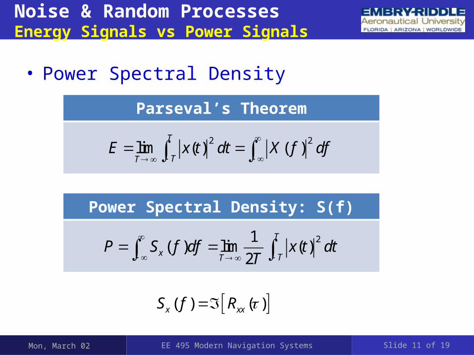
Parseval’s Theorem

2 2lim ( ) ( )

T

TTE x t dt X f df

Power Spectral Density: S(f)

21( ) lim ( )

2

T

x TTP S f df x t dt

T

• Power Spectral Density

( ) ( )x xxS f R

Slide 11 of 19




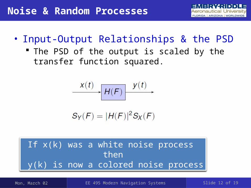
• Input-Output Relationships & the PSD The PSD of the output is scaled by the transfer function

squared.

If x(k) was a white noise process then

y(k) is now a colored noise process

Slide 12 of 19


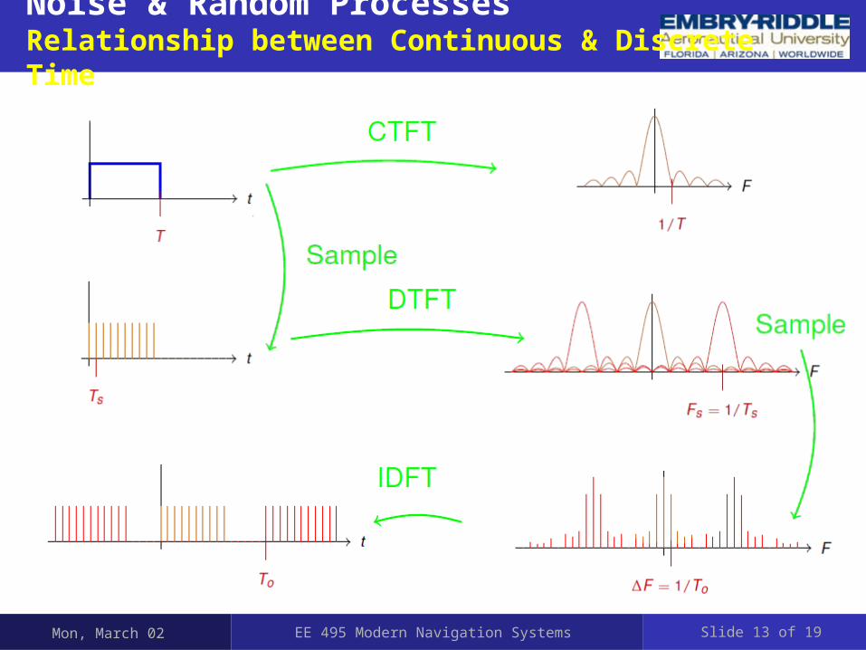
Noise & Random ProcessesRelationship between Continuous & Discrete Time

Mon, March 02 EE 495 Modern Navigation Systems Slide 13 of 19




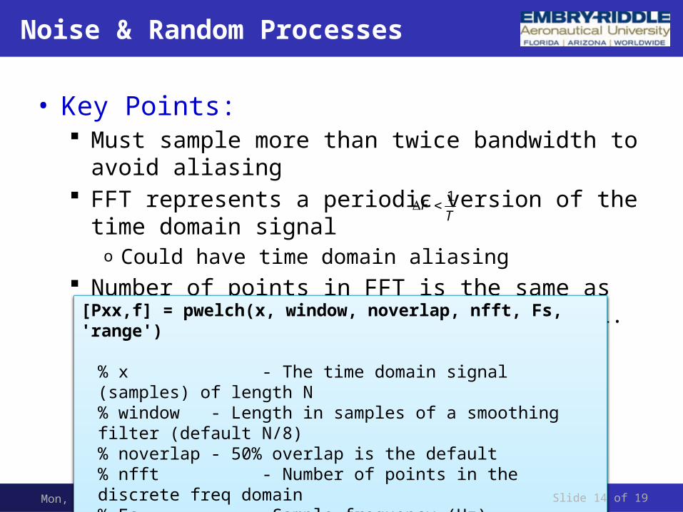
• Key Points: Must sample more than twice bandwidth to avoid aliasing FFT represents a periodic version of the time domain signal

o Could have time domain aliasing Number of points in FFT is the same as number of points in

time domain signal.

[Pxx,f] = pwelch(x, window, noverlap, nfft, Fs, 'range')

% x - The time domain signal (samples) of length N% window - Length in samples of a smoothing filter (default N/8)% noverlap - 50% overlap is the default% nfft - Number of points in the discrete freq domain% Fs - Sample frequency (Hz)% range - Two-sided or one-sided frequency range

Slide 14 of 19

1F

T


0 50 100 150 200 250 300 350 400 450 5000

0.05

0.1

0.15

0.2

0.25

Freq (Hz)

PS

D

Power Spectral Density (Pxx

)



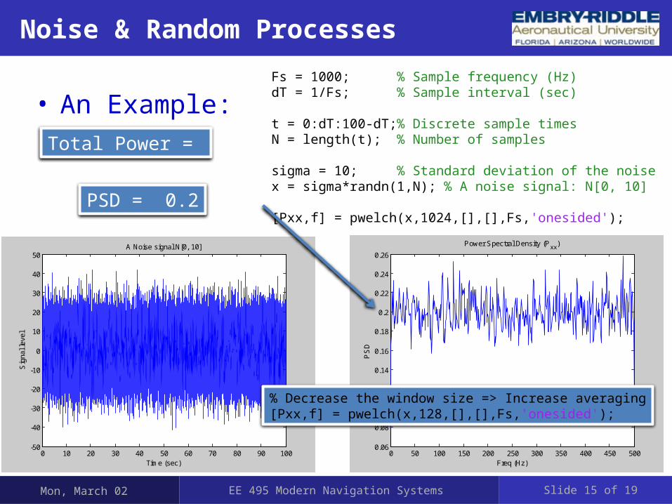
• An Example:Fs = 1000; % Sample frequency (Hz)dT = 1/Fs; % Sample interval (sec) t = 0:dT:100-dT;% Discrete sample timesN = length(t); % Number of samples sigma = 10; % Standard deviation of the noisex = sigma*randn(1,N); % A noise signal: N[0, 10]

[Pxx,f] = pwelch(x,1024,[],[],Fs,'onesided');

0 10 20 30 40 50 60 70 80 90 100-50

-40

-30

-20

-10

0

10

20

30

40

50

Time (sec)

Sig

nal l

evel

A Noise signal N[0, 10]

0 50 100 150 200 250 300 350 400 450 5000.06

0.08

0.1

0.12

0.14

0.16

0.18

0.2

0.22

0.24

0.26

Freq (Hz)

PS

D


)

Total Power =

% Decrease the window size => Increase averaging[Pxx,f] = pwelch(x,128,[],[],Fs,'onesided');

PSD = 0.2

Slide 15 of 19




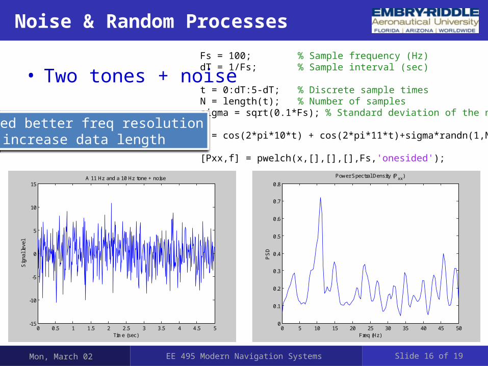
• Two tones + noiseFs = 100; % Sample frequency (Hz)dT = 1/Fs; % Sample interval (sec) t = 0:dT:5-dT; % Discrete sample timesN = length(t); % Number of samplessigma = sqrt(0.1*Fs); % Standard deviation of the noise x = cos(2*pi*10*t) + cos(2*pi*11*t)+sigma*randn(1,N);

[Pxx,f] = pwelch(x,[],[],[],Fs,'onesided');

0 5 10 15 20 25 30 35 40 45 500

0.1

0.2

0.3

0.4

0.5

0.6

0.7

0.8

Freq (Hz)

PS

D


)

Need better freq resolution increase data length

0 0.5 1 1.5 2 2.5 3 3.5 4 4.5 5-15

-10

-5

0

5

10

15

Time (sec)

Sig

nal l

evel

A 11 Hz and a 10 Hz tone + noise

Slide 16 of 19




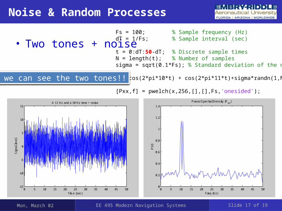
• Two tones + noiseFs = 100; % Sample frequency (Hz)dT = 1/Fs; % Sample interval (sec) t = 0:dT:50-dT; % Discrete sample timesN = length(t); % Number of samplessigma = sqrt(0.1*Fs); % Standard deviation of the noise x = cos(2*pi*10*t) + cos(2*pi*11*t)+sigma*randn(1,N);

[Pxx,f] = pwelch(x,256,[],[],Fs,'onesided');

Now we can see the two tones!!

0 5 10 15 20 25 30 35 40 45 50-15

-10

-5

0

5

10

15

Time (sec)

Sig

nal l

evel

A 11 Hz and a 10 Hz tone + noise

0 5 10 15 20 25 30 35 40 45 500

0.2

0.4

0.6

0.8

1

1.2

1.4

Freq (Hz)

PS

D


)

Slide 17 of 19


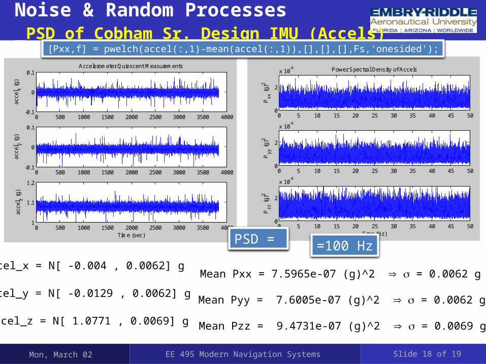
Noise & Random Processes_PSD of Cobham Sr. Design IMU (Accels)


0 5 10 15 20 25 30 35 40 45 500

2

x 10-6

Pxx

(g)

2

Power Spectral Density of Accels

0 5 10 15 20 25 30 35 40 45 500

2

x 10-6

Pyy

(g)

2

0 5 10 15 20 25 30 35 40 45 500

2

x 10-6

Freq (Hz)

Pzz

(g)

2

0 500 1000 1500 2000 2500 3000 3500 4000-0.1

0

0.1

acce

l x (g)

Accelerometer Quiescent Measurements

0 500 1000 1500 2000 2500 3000 3500 4000-0.1

0

0.1

acce

l y (g)

0 500 1000 1500 2000 2500 3000 3500 40001

1.1

1.2

acce

l z (g)

Time (sec)

Accel_x = N[ -0.004 , 0.0062] g

Accel_y = N[ -0.0129 , 0.0062] g

Accel_z = N[ 1.0771 , 0.0069] g

Mean Pxx = 7.5965e-07 (g)^2 = 0.0062 g

PSD =

Mean Pyy = 7.6005e-07 (g)^2 = 0.0062 g

Mean Pzz = 9.4731e-07 (g)^2 = 0.0069 g

[Pxx,f] = pwelch(accel(:,1)-mean(accel(:,1)),[],[],[],Fs,'onesided');

Slide 18 of 19

=100 Hz


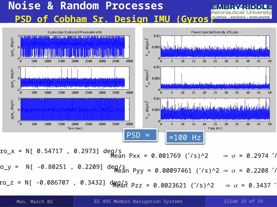
Noise & Random Processes_PSD of Cobham Sr. Design IMU (Gyros)


0 5 10 15 20 25 30 35 40 45 500

0.005

0.01

Pxx

(de

g/s)

2

Power Spectral Density of Gyros

0 5 10 15 20 25 30 35 40 45 500

0.005

0.01

Pyy

(de

g/s)

2

0 5 10 15 20 25 30 35 40 45 500

0.005

0.01

Freq (Hz)

Pzz

(de

g/s)

2

0 500 1000 1500 2000 2500 3000 3500 4000-2

0

2

gyro

x (de

g/s)

Gyroscope Quiescent Measurements

0 500 1000 1500 2000 2500 3000 3500 4000-2

0

2

gyro

y (de

g/s)

0 500 1000 1500 2000 2500 3000 3500 4000-2

0

2

gyro

z (de

g/s)

Time (sec)

Gyro_x = N[ 0.54717 , 0.2973] deg/s

Gyro_y = N[ -0.80251 , 0.2209] deg/s

Gyro_z = N[ -0.086707 , 0.3432] deg/s

Mean Pxx = 0.001769 (/s)^2 = 0.2974 /s

Mean Pyy = 0.00097461 (/s)^2 = 0.2208 /s

Mean Pzz = 0.0023621 (/s)^2 = 0.3437 /s

PSD =

Slide 19 of 19

=100 Hz


ee 495 modern navigation systems noise & random processes mon, march 02 ee 495 modern navigation...

Documents