economics tutorial - university of california, berkeleyeecsba1/sp97/slides/lect12a.pdf · here we...

Copyright 1997, David G. Messerschmitt. All rights reserved.

Here we give a quick tutorial on the economics material that has been covered in class.

For further information, the book

Hal Varian, Intermediate Economics, A Modern Approach. New York, Norton, Fourth Edition, 1996.

is recommended. If you are willing to purchase the book, I am sure one of the instructors will be pleased!

Copyright 1997, David G. Messerschmitt 3/5/97 1

Economics tutorialEconomics tutorial

David G. MesserschmittDavid G. Messerschmitt

CS 294-6, EE 290X, BA 296.5CS 294-6, EE 290X, BA 296.5


A “consumption bundle” is a particular quantity (x,y) of widgets and what’sits.

It is convenient to define a utility function u(x,y), with the interpretation that a consumption bundle (x,y) with a higher utility is preferred to one with a smaller utility. No particular significance is attached to the numerical value of u(x,y), it simply defines an ordering relationship of conumption bundles which we interpret as consumer preference. That is, we do not interpret a doubling of utility as a doubling of preference, or a doubling of acceptable price, or anything like that. The utility function is thus not unique; for example the square root of the utility function or the logarithm of the utility functions represent exactly the same consumer preference.

The indifference curve is defined as

u(x,y) = constant

where the constant is presumed to increase as we move toward larger consumption bundles. A larger constant represents a larger preference.

We have shown the case where the indifference curves are convex, which means that the weighted average of two consumption bundles is preferred to either of the bundles alone. This is typical, but not necessary. (For example, either ice cream or olives alone would likely be preferred to their mixture.)


Consumer preferencesConsumer preferences

Quantity ofwhat’sits y

Quantity ofwidgets x

Consumer is indifferent to any“consumption bundle” (x,y) on this curve

Increasing preference


Instead of letting the vertical axis y be the quantity of what’sits consumed, let it be the total dollars spent on goods other than widgets.

Presume that the price charged per unit of widget is p, and the consumer’s total income ($ available to spend on all goods) is m. Then we must have that

m = y + p*x

This is called the consumer’s budget line. The y-intercept of this line is m, and the slope is the negative of p.

At the consumption bundle that maximizes the consumer’s utility and also falls on the budget line, the budget line will be tangent to an indifference curve.

For the case shown, as is typical, the quantity of widgets consumed x will increase (move to the right) as the income m increases.


Budget lineBudget line

$ spent on allother goods y


IncomeSlope is negativeof price charged per unitof widget

Consumer preference ismaximized


Quasilinear preferences is a special case of a utility function for which

u(x,y) = v(x) + y

That is, the consumer’s utility increases linearly with y (the $ available to spend on all other goods).

The indifference curve is given by

u(x,y) = constant or y = constant - v(x)

Thus, the indifference curves all have the same shape v(x) and are just vertically shifted versions of one another. For this special case, the optimum consumption bundle has a very special property: The consumption of widgets, x, does not depend on income m for any fixed price p. (This is because the slope of the indifference curve will equal p at a value of x that is independent of m.) Thus, this case models the situation where your consumption of widgets doesn’t depend on your income. This is probably a pretty good assumption for pencil widgets, and a bad assumption for BMW widgets.

For this special case, we can easily find the price vs. quantity that the consumer will buy at that price. Substituting for the budget line, the utility is

u(x,y) = v(x) + m - px

Taking the derivative and setting to zero, a condition for maximizing utility is

v’(x) - p = 0 or p(x) = v’(x)

p(x) vs. x is called the inverse demand function.


Quasilinear prefrencesQuasilinear prefrences

$ spent on allother goods y


Special case: indifference curvesare vertical shifts of one another

Consumption of widgetsdoes not depend on income


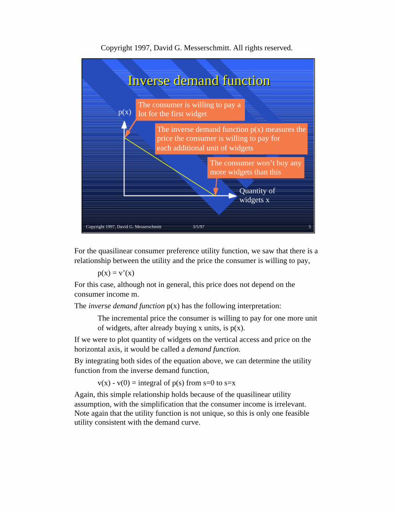
For the quasilinear consumer preference utility function, we saw that there is a relationship between the utility and the price the consumer is willing to pay,

p(x) = v’(x)

For this case, although not in general, this price does not depend on the consumer income m.

The inverse demand function p(x) has the following interpretation:

The incremental price the consumer is willing to pay for one more unit of widgets, after already buying x units, is p(x).

If we were to plot quantity of widgets on the vertical access and price on the horizontal axis, it would be called a demand function.

By integrating both sides of the equation above, we can determine the utility function from the inverse demand function,

v(x) - v(0) = integral of p(s) from s=0 to s=x

Again, this simple relationship holds because of the quasilinear utility assumption, with the simplification that the consumer income is irrelevant. Note again that the utility function is not unique, so this is only one feasible utility consistent with the demand curve.


Inverse demand functionInverse demand function

p(x)


The inverse demand function p(x) measures theprice the consumer is willing to pay foreach additional unit of widgets

The consumer won’t buy any more widgets than this

The consumer is willing to pay a lot for the first widget


The assumption of a fixed price is a common case. Alternative pricing strategies would be to sell different versions at different prices (covered later), or provide a quantity discount (charge more per unit widget as the total widgets purchased gets larger).


Quantity consumed vs. price Quantity consumed vs. price chargedcharged

p(x)


Assume the producer of widgetscharges a fixed price p

p

The consumer is just indifferentto buying one more unit

The consumer will buy thisquantity of widgets


With the fixed price strategy, the producer revenue is p*x, where x is the quantity sold.

If we were able to charge as much for each unit of widget as the consumer were willing to pay, the producer could derive a revenue of

revenue = integral from s=0 to s=x of p(x)

The difference between this maximum feasible revenue and the fixed-price revenue is the area in red, and is called the consumer’s surplus. This is the revenue the producer has foregone by selling widgets at a fixed price.

Looking at it from the consumer’s perspective, she has derived more value in buying widgets than she paid! That is, she paid less than she was willing to pay.

If we were to pay the consumer not to consume widgets, we would have to pay her an amount equal to the consumer’s surplus to induce her to not buy widgets.


Consumer surplusConsumer surplus

p(x)


p

Consumer surplus is what we would have topay the consumer not to consume widgets


Now we consider a more complicated model that often applies to communications and computing products, especially networked applications and many software products.

We presume that the inverse demand function p(x,n) is not only a function of the quantity consumed x, but also n, the number of widgets that the consumer expects to be sold. We presume that the inverse demand function is larger when n is larger; that is, the consumers are willing to pay more when there are more widgets consumed in total.

A good example would be facsimile machine widgets. A facsimile machine is worth more to you (presuming you want to send fax’es at all) when there are more facsimile machines sold in total.

In this diagram, x is presumed to be the total quantity of widgets sold, not the number sold to one consumer. Similarly p is the price the aggregate of consumers is willing to pay for the next unit of widgets.


Network externalityNetwork externalityp(x,n)


large n

small n

Willingness to pay for the x-thunit of widget when n widgets are expected to be sold in total


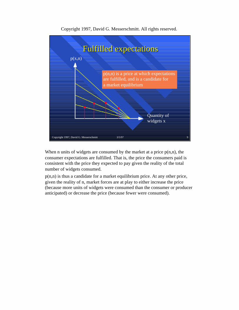
When n units of widgets are consumed by the market at a price p(n,n), the consumer expectations are fulfilled. That is, the price the consumers paid is consistent with the price they expected to pay given the reality of the total number of widgets consumed.

p(n,n) is thus a candidate for a market equilibrium price. At any other price, given the reality of n, market forces are at play to either increase the price (because more units of widgets were consumed than the consumer or producer anticipated) or decrease the price (because fewer were consumed).


Fulfilled expectationsFulfilled expectationsp(x,n)


p(n,n) is a price at which expectations are fulfilled, and is a candidate fora market equilibrium


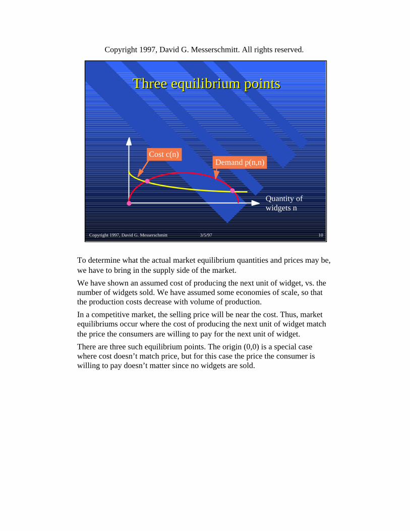
To determine what the actual market equilibrium quantities and prices may be, we have to bring in the supply side of the market.

We have shown an assumed cost of producing the next unit of widget, vs. the number of widgets sold. We have assumed some economies of scale, so that the production costs decrease with volume of production.

In a competitive market, the selling price will be near the cost. Thus, market equilibriums occur where the cost of producing the next unit of widget match the price the consumers are willing to pay for the next unit of widget.

There are three such equilibrium points. The origin (0,0) is a special case where cost doesn’t match price, but for this case the price the consumer is willing to pay doesn’t matter since no widgets are sold.


Three equilibrium pointsThree equilibrium points

Quantity ofwidgets n

Demand p(n,n)Cost c(n)


We can anticipate the direction that market forces will drive us in each of the three regions.

For small quantities, the producer cost exceeds the consumer willingness to pay. The willingness to pay is low because the consumer expects few widgets to be sold, and thus widgets are less valuable because of the externality. The quantity sold would be expected to reduce with time, because cost exceeds price.

In the middle region, which we call self sustaining, willingness to pay exceeds producer cost, and hence consumption will increase with time.

In the highest quantity region, we are reaching market saturation where the willingness to pay is again less than production costs, because consumers are have has many widgets as they can reasonably utilize. (For example, all the people who want to send fax’es already have a facsimile machine.) Here, the quantity consumed tends to decrease.

Thus, there are two stable equilibrium points, and one unstable.

The question we have to answer in establishing a new product in the presence of externalities is how do we move the market into the self-sustaining region? Generally this requires some subsidy of the consumers, either from the producers or from government regulation.


DynamicsDynamics

Quantity ofwidgets n

unstablestable

stable


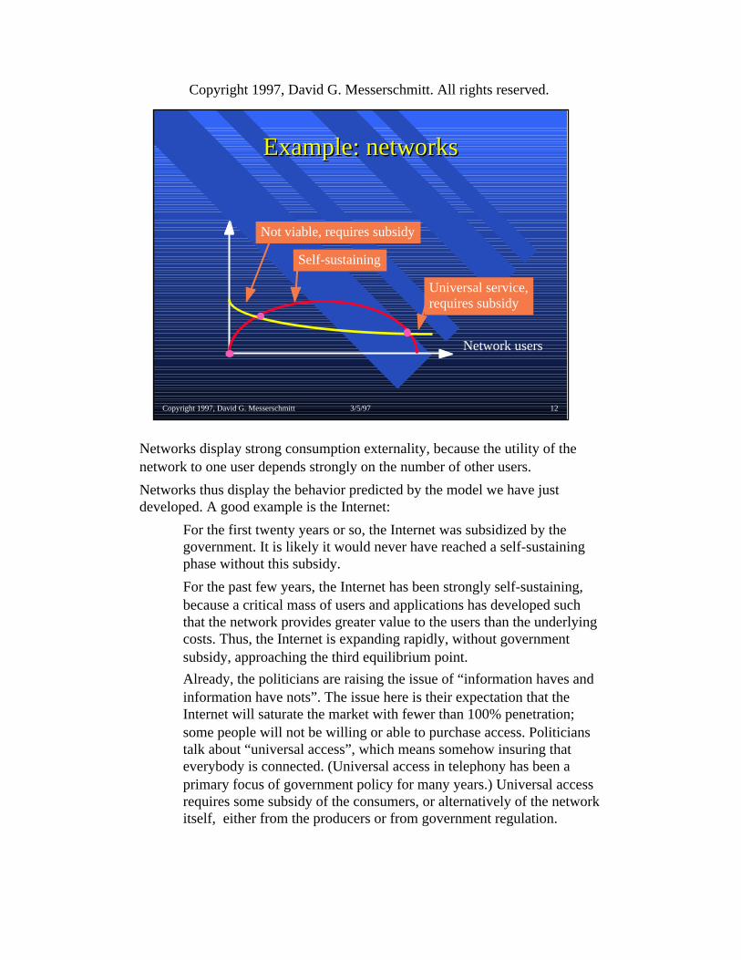
Networks display strong consumption externality, because the utility of the network to one user depends strongly on the number of other users.

Networks thus display the behavior predicted by the model we have just developed. A good example is the Internet:

For the first twenty years or so, the Internet was subsidized by the government. It is likely it would never have reached a self-sustaining phase without this subsidy.

For the past few years, the Internet has been strongly self-sustaining, because a critical mass of users and applications has developed such that the network provides greater value to the users than the underlying costs. Thus, the Internet is expanding rapidly, without government subsidy, approaching the third equilibrium point.

Already, the politicians are raising the issue of “information haves and information have nots”. The issue here is their expectation that the Internet will saturate the market with fewer than 100% penetration; some people will not be willing or able to purchase access. Politicians talk about “universal access”, which means somehow insuring that everybody is connected. (Universal access in telephony has been a primary focus of government policy for many years.) Universal access requires some subsidy of the consumers, or alternatively of the network itself, either from the producers or from government regulation.


Example: networksExample: networks

Network users

Self-sustaining

Universal service,requires subsidy

Not viable, requires subsidy


We can replace quantity by quality, resulting in the inverse quality demand curve. This curve indicates the incremental price the consumer is willing to pay for the next unit increment in quality.

This curve presumes quality is a continuous function; in fact, in practice it is more likely to be discrete.


Quality demand curveQuality demand curve

p(x)

Quality ofwidgets x

The quality inverse demand function determines the incremental price the consumer is willing to pay for one more unit of quality


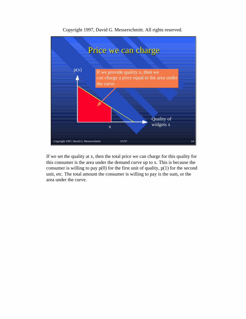
If we set the quality at x, then the total price we can charge for this quality for this consumer is the area under the demand curve up to x. This is because the consumer is willing to pay p(0) for the first unit of quality, p(1) for the second unit, etc. The total amount the consumer is willing to pay is the sum, or the area under the curve.


Price we can chargePrice we can charge

p(x)

Quality ofwidgets x

If we provide quality x, then wecan charge a price equal to the area underthe curve

x


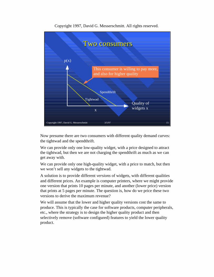
Now presume there are two consumers with different quality demand curves: the tightwad and the spendthrift.

We can provide only one low-quality widget, with a price designed to attract the tightwad, but then we are not charging the spendthrift as much as we can get away with.

We can provide only one high-quality widget, with a price to match, but then we won’t sell any widgets to the tightwad.

A solution is to provide different versions of widgets, with different qualities and different prices. An example is computer printers, where we might provide one version that prints 10 pages per minute, and another (lower price) version that prints at 5 pages per minute. The question is, how do we price these two versions to derive the maximum revenue?

We will assume that the lower and higher quality versions cost the same to produce. This is typically the case for software products, computer peripherals, etc., where the strategy is to design the higher quality product and then selectively remove (software configured) features to yield the lower quality product.


Two consumersTwo consumers

p(x)

Quality ofwidgets xx

This consumer is willing to pay more,and also for higher quality

Spendthrift

Tightwad


One approach is to make the lower-quality version of the widget the highest quality the tightwad is willing to pay for, charging him the amount shown in red.


Catering to the tightwad Catering to the tightwad consumerconsumer

p(x)

Quality ofwidgets x

To cater to the tightwad,our price is the area shown atthis quality (or any higher quality)


If this is the only version we offer, the spendthrift consumer will buy it, but we will leave the surplus shown in yellow.

This surplus prevents us from charging the maximum price for the high-quality version, since the spendthrift will be left with no consumer surplus if we were to do that.


Spendthrift consumer surplusSpendthrift consumer surplus

p(x)

Quality ofwidgets x

Unfortunately, we leave thisconsumer surplus with the spendthrift,the value she derives above what shepays


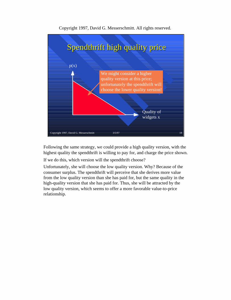
Following the same strategy, we could provide a high quality version, with the highest quality the spendthrift is willing to pay for, and charge the price shown.

If we do this, which version will the spendthrift choose?

Unfortunately, she will choose the low quality version. Why? Because of the consumer surplus. The spendthrift will perceive that she derives more value from the low quality version than she has paid for, but the same quality in the high-quality version that she has paid for. Thus, she will be attracted by the low quality version, which seems to offer a more favorable value-to-price relationship.


Spendthrift high quality priceSpendthrift high quality price

p(x)

Quality ofwidgets x

We might consider a higherquality version at this price;unfortunately the spendthrift willchoose the lower quality version!


A price that will attract the spendthrift to the high quality version is the area shown in red. This is bacause the consumer surplus is the same as for the low quality version. Thus, the spendthrift perceives the high quality version as offering a value that exceeds price by the same amount as the low quality version. Thus, she will choose the high quality version.


Higher quality version for the Higher quality version for the spendthriftspendthrift

p(x)

Quality ofwidgets x

We can charge the spendthriftthis much for the highquality version without affecting her consumer surplus


We can increase our total revenues even further by lowering the quality of the lower-quality version. We can sell to the tightwad at the price shown. The advantage is that this reduces the consumer surplus of the spendthrift, when she purchases the low-quality version, allowing us to charge the spendthrift more for the high-quality version.

Thus, we get less revenue from the tightwad, but more from the spendthrift. Clearly there is an optimum point (to maximize revenues) where these just balance.


Reduce quality of low-quality Reduce quality of low-quality versionversion

p(x)

Quality ofwidgets x

Lowering quality will derive less revenue from the tightwad


This is what we can charge the spendthrift at the highest quality she will pay for. We can now set the quality of the low-quality version at the point where we derive the highest revenue. This optimum point will depend on the relative number of tightwad and spendthrift consumers.


Charge more for the high-quality Charge more for the high-quality versionversion

p(x)

Quality ofwidgets x

We can charge the spendthrift this much, perhaps increasing our total revenue on net

economics tutorial - university of california, berkeleyeecsba1/sp97/slides/lect12a.pdf · here we...

Documents