economic volatility and returns to education in venezuela

Economic Volatility and Returns to Education in Venezuela: 1992-2002

Harry Anthony Patrinos* World Bank

Washington DC [email protected]

Chris Sakellariou∗ School of Humanities and Social Sciences

Nanyang Technological University, Singapore [email protected]

Abstract: Preliminary evidence suggests that the rates of return to education in Venezuela have been declining since the 1970s. This paper rigorously estimates the returns to education in Venezuela for the period 1992-2002 and links them to earlier available estimates from the 1980s. Consistent cross-sections from the Encuesta de Hogares por Muestro are used to document falling returns to schooling and educational levels until the mid-1990s, followed by increasing returns thereafter. Quantile regression analysis is used to provide further insight into the within skill group changes in returns over time. JEL Classification Codes: I21, J31 Keywords: Returns to schooling, wages, quantile regressions World Bank Policy Research Working Paper 3459, November 2004 The Policy Research Working Paper Series disseminates the findings of work in progress to encourage the exchange of ideas about development issues. An objective of the series is to get the findings out quickly, even if the presentations are less than fully polished. The papers carry the names of the authors and should be cited accordingly. The findings, interpretations, and conclusions expressed in this paper are entirely those of the authors. They do not necessarily represent the view of the World Bank, its Executive Directors, or the countries they represent. Policy Research Working Papers are available online at http://econ.worldbank.org.

∗ The authors would like to thank Emiliana Vegas and George Psacharopoulos for useful comments, as well as discussants and participants at the Latin America and the Caribbean Economic Association meetings, Puebla, Mexico, October 2003.

Pub

lic D

iscl

osur

e A

utho

rized

Pub

lic D

iscl

osur

e A

utho

rized

Pub

lic D

iscl

osur

e A

utho

rized

Pub

lic D

iscl

osur

e A

utho

rized

Administrator

WPS3459

1. Introduction

Measures of inequality with respect to education and skills have changed, sometimes

dramatically, over the last two decades. Increasing skill differentials have been clearly observed

for the United States and, to a lesser extent, other developed countries such as Portugal, Denmark

and Italy, while falling returns have been documented for Sweden and, recently, Austria (see

Asplund and Pereira 1999; Harmon and others 2001; Fersterer and Winter-Ebmer 2003; see

Psacharopoulos and Patrinos 2004 for a review of studies). Evidence for developing countries is

scarce. One can hypothesize that significant developments in the returns to education and skills

have taken place in the developing world, given the volatility in the evolution of incomes and

poverty in many developing countries.

Venezuela experienced a significant increase in poverty incidence during the 1980s

(especially during the recessionary period from 1982 to 1985). Poverty followed a decreasing

trend until 1992, after a 3-year period of growth, bringing poverty incidence to pre-1985 levels.

Post-1992 stagnant growth, however, resulted in poverty levels resuming an ascending path

(Mosconi and Alvarez 1996). During the 1990s, economic performance exhibited sharp

fluctuations, with a year of strong growth usually followed by a sharp decline one or two years

later. This pattern seems to be continuing into the next decade.

In Venezuela, while there has been a consistent increase in the overall level of schooling

of the labor force since the mid-1970s, the returns to schooling have decreased over time, but in

the last two years have started to increase again. This suggests that until recently the supply of

human capital in the labor market has been expanding at a faster rate than has the demand for

2

human capital, thereby lowering the rate of return to schooling. The results for Venezuela in the

first two years of the new century are in line with what happened in other middle-income

countries in Latin America in the 1990s – such as Mexico, Brazil and Chile (see for example

Blom and others 2001; Lachler 1998) – where the returns to secondary and tertiary education

increased over time, and where the overall rate of return to schooling also increased. It signals

that the demand for educated labor was not increasing in Venezuela in the 1990s, most likely due

to the economic downturn, but that in the last two years education has become more profitable.

2. Data

We use consistent cross-sections from the Encuesta de Hogares por Muestro conducted

by the National Statistical Office of Venezuela (OCEI). The data used are for survey years 1992,

1995, 1996, 1997, 1998, 1999 and 2000. The survey instrument for 1992 involved a shorter

questionnaire compared to post-1992 questionnaires but a much larger sample (over 300,000

observations for 1992 compared to about 65,000-80,000 in later surveys).

The working sub-sample used in this study in deriving returns to an additional year of

schooling and education levels, as well as returns by quantile, consists of workers aged 15-65,

working for wages.

3

3. Results

Educational attainment in Venezuela, measured by the years of completed education of

the selected sub-sample, has been increasing steadily from 4.6 years in 1975 to 8.2 years in the

mid-1990s. Subsequently the increase has been rather slow and by the year 2002 it stood at 8.9

years (Table 1). Women complete more years of education than men and this was the case for

every year examined. In year 2002, women who were employed for wages in Venezuela

completed, on average, 10.1 years of education compared to 8.3 years for men. Furthermore the

education gap by sex seemed to be widening during the 1990s, increasing from about 1.1 years in

1992, to 1.5 in 1996 and to 1.8 in 2002.

In deriving returns to education, we use the earnings function method (Mincer 1974),

which involves the fitting of a function specified as:

lnYi = α + βSi + γ1EXi + γ2EX2i + γ3Zi + εi,

where lnY is the natural logarithm of monthly earnings, S is the number of years of schooling of

individual i, EX and EX2 are the years of experience and its square, and Z is a vector of control

variables comprising compensatory factors. For purposes of comparison with other similar

studies and earlier results for Venezuela, only one compensatory variable is used, namely the

natural logarithm of monthly working hours. In this semi-log specification, the coefficient on S

(β) is interpreted as the private rate of return to one additional year of schooling, averaged across

all levels of education and all individuals in the sample. For small values of β (say, 0.10 or less),

applying the rule regarding natural logarithms results in values of the rate of return to schooling

within a fraction of 1 percent of the derived coefficient, β.

4

The earnings function method is also used to estimate returns to different levels of

schooling, by converting the continuous years of schooling variable into a series of dummy

variables representing the levels of schooling. After fitting the extended earnings function:

lnYi = α + β1PRIMi + β2SECi + β3HIGHER + β4UNIVi + γ1EXi + γ2 EX2i +γ3Zi + εi,

where PRIM, SEC, HIGHER and UNIV refer to dummy variables for primary, secondary, higher

and university education, from the formulas:

r(PRIM) = β1 / SPRIM

r(SEC) = (β2 – β1) / (SSEC - SPRIM)

r(HIGHER) = (β3 – β2) / (SHIGHER – SSEC)

r(UNIV) = (β 4– β2) / (SUNIV – SSEC)

where SPRIM, SSEC, SHIGHER and SUNIV are the total number of years of schooling for each

successive level of education. However, it is incorrect to assume that primary school graduates

forego earnings for the entire duration of their studies. Therefore, only three years of foregone

earnings for primary school graduates are assumed.

Mincerian earnings functions are estimated for men and women, and estimates with

sample selection for women, using Heckman’s two-step procedure, which involves an earnings

equation (see Annex Table 1):

LnYi = Xiβi + σεviλi + εi,

and a participation equation:

Ii = (θ’izi + vi > 0),

where λi is a vector of inverse Mills’ ratios, with parameters derived from a probit model which

models the determinants of labor market participation. X and Z are vectors of explanatory

5

variables, β and θ are vectors of coefficients, ε and v are the disturbance terms of the earnings

and selection equations, and σεvi is the covariance of the two error terms. Female labor force

participation in Venezuela has been steadily increasing during the 1990s, from about 50 percent

in 1992 to 63.2 percent in 2002. The pattern of employment of women, with respect of sector of

employment is similar to that of men.

Table 1: Returns to Schooling and Average Years of Schooling by Sex: 1975-2002

Rate of Return (%) All Men Women ( corrected for selectivity)

Average Years of Schooling All Men Women

1975* 13.7 - - 4.6 - - 1984* 11.2 - - 6.6 - - 1987* 10.7 10.0 13.1 6.9 - - 1989* 9.6 9.4 11.3 7.7 - - 1992 8.8 8.4 11.9 8.0 7.6 8.7 1995 8.0 8.0 9.6 8.2 7.7 9.1 1996 7.6 7.4 10.1 8.4 7.9 9.4 1997 9.2 9.1 11.7 8.3 7.8 9.3 1998 9.0 9.2 10.5 8.7 8.0 9.9 1999 9.2 9.1 11.9 8.7 8.0 9.9 2000 8.0 7.9 9.4 8.7 8.0 9.9 2001 9.4 9.1 11.3 8.8 8.1 10.0 2002 10.4 9.9 12.7 8.9 8.3 10.1 Sources: Psacharopoulos and Alam 1991; Fiszbein and Psacharopoulos 1993; Psacharopoulos

and Steier 1988; authors’ estimates for 1992-2002

The overall return to one additional years of schooling steadily declined in the 1970s,

1980s and through the mid-1990s (Table 1). The benefits decline from 13.7 percent in 1975 to 8

percent in 1995, and 7.6 percent in 1996. Since then, returns have exhibited an increasing trend,

reaching 9.4 percent in 2001 and 10.4 percent in 2002. Returns for men are consistently lower

than returns for women and the difference in returns has been between 1.3 (in 1998) and 3.0 (in

1992) percentage points.

6

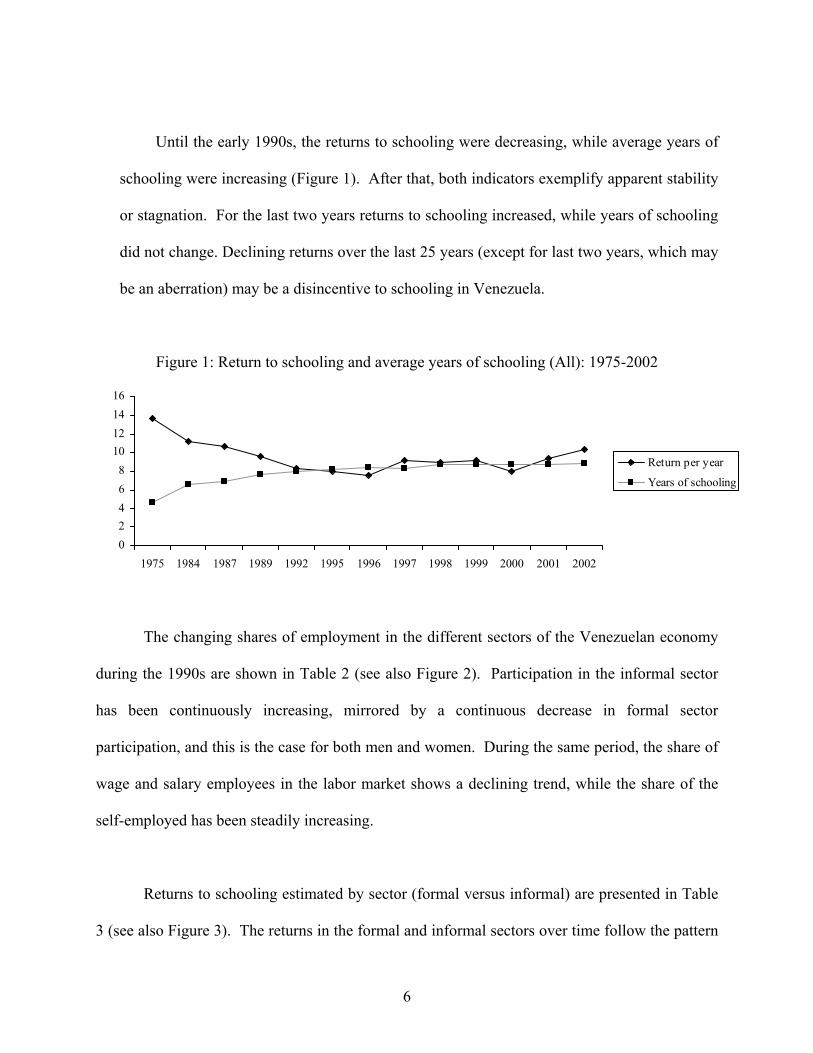
Until the early 1990s, the returns to schooling were decreasing, while average years of

schooling were increasing (Figure 1). After that, both indicators exemplify apparent stability

or stagnation. For the last two years returns to schooling increased, while years of schooling

did not change. Declining returns over the last 25 years (except for last two years, which may

be an aberration) may be a disincentive to schooling in Venezuela.

Figure 1: Return to schooling and average years of schooling (All): 1975-2002

02468

10121416

1975 1984 1987 1989 1992 1995 1996 1997 1998 1999 2000 2001 2002

Return per year

Years of schooling

The changing shares of employment in the different sectors of the Venezuelan economy

during the 1990s are shown in Table 2 (see also Figure 2). Participation in the informal sector

has been continuously increasing, mirrored by a continuous decrease in formal sector

participation, and this is the case for both men and women. During the same period, the share of

wage and salary employees in the labor market shows a declining trend, while the share of the

self-employed has been steadily increasing.

Returns to schooling estimated by sector (formal versus informal) are presented in Table

3 (see also Figure 3). The returns in the formal and informal sectors over time follow the pattern

7

of the overall returns, showing considerable decline. Returns in the informal sector exhibit less

variability, ranging from only 5.7 to 7.3 percent during the whole ten year period. Returns in the

formal sector are higher than returns in the informal sector and the spread is increasing after

1996.

Table 2: Shares of Sectors of Employment: 1992-2002 Formal Informal Employees Self-employed 1992 65.3 34.7 71.4 19.9 1995 54.5 45.5 67.8 26.9 1996 54.9 45.1 67.3 27.6 1997 53.1 46.9 68.1 26.6 1998 51.1 48.9 64.9 29.5 1999 49.2 50.8 62.3 31.2 2000 48.0 52.0 60.5 33.1 2001 47.6 52.4 60.8 29.9 2002 46.0 54.0 62.4 29.3 Source: Encuesta de Hogares por Muestro

Figure 2: Shares of employment for Informal Sector, Employees and Self-employed: 1992-2002

0

10

20

30

40

50

60

70

80

1992 1995 1996 1997 1998 1999 2000 2001 2002

InformalEmployeesSelf-employed

8

Table 3: Returns to schooling (Mincer Equations) by sector*: Formal vs Informal, 1992-2002 Formal

All Men Women Informal

All Men Women1992 8.8 8.9 9.7 6.5 5.8 8.2 1995 7.0 7.4 7.9 7.3 7.3 7.7 1996 7.1 7.1 8.9 6.9 7.2 7.5 1997 8.5 8.6 10.0 6.8 7.3 7.3 1998 9.1 9.3 10.7 7.0 7.9 6.8 1999 8.8 9.1 10.2 6.5 7.0 6.7 2000 7.0 7.2 7.9 5.7 6.3 5.7 2001 8.6 8.4 10.6 6.2 6.8 6.4 2002 9.7 9.4 11.7 6.7 7.4 6.6 Source: Encuesta de Hogares por Muestro * All sectors of employment included in the sample

Figure 3: Rates of return by sector (formal vs informal): 1992-2002

0

2

46

8

10

12

1992 1995 1996 1997 1998 1999 2000 2001 2002

Formal

Informal

To complement the results on the returns to schooling, we look at education premiums by

level and sex (see Annex Table 2). The interest here is to document which levels are associated

with falling earnings premiums over time and whether the developments are similar for both

males and females. Since there is very little evidence of sample selection in Venezuela, rates of

return to education by level were derived from OLS regressions.

9

Overall the results follow the trend observed in the results on returns to schooling (see

Table 4). Primary and secondary premiums are relatively stable during the decade for both men

and women, while university premiums are more volatile, exhibiting a falling trend from 1996 to

2000 and an increasing trend thereafter. Females, with few exceptions, enjoy higher education

premiums compared to males for all education levels. Premiums for secondary education

(compared to primary) are of comparable magnitude to primary premiums (compared to no

education), with primary premiums being slightly higher than secondary premiums. University

premiums (compared to secondary) for males mirror the developments in male returns to

schooling. They declined from 0.62 in 1992 to 0.40 in 1995, rebounded in 1996, and

subsequently declined for the 1997-2000 period, before increasing again in 2001 and 2002.

The reasons for the observed developments in returns to schooling and education

premiums relate to changes in the supply of more educated workers which, depending on

economic activity, may or may not be compensated by a corresponding demand for skills.

During the 1990s, the Venezuelan economy was characterized by: (a) sharp fluctuations in

economic activity; (b) volatile but, overall, decreasing real incomes; and (c) a steady increase in

poverty. During the same period, a lack of opportunities in the formal sector resulted in an

increasing number of workers moving into the informal sector, where returns to education are

low and poverty is endemic.

Returns to Schooling and Real Wages

There is a close association between real wages and returns to schooling in Venezuela

(Figure 4). It suggests that the overall return to schooling has been shaped by the effects of

10

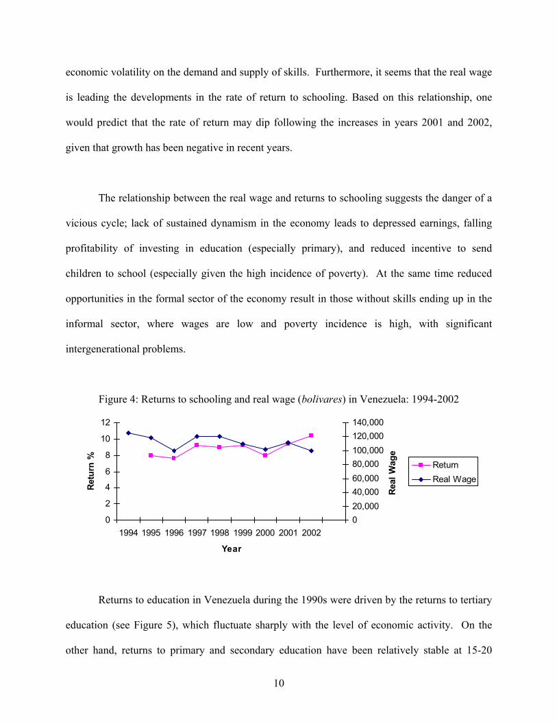
economic volatility on the demand and supply of skills. Furthermore, it seems that the real wage

is leading the developments in the rate of return to schooling. Based on this relationship, one

would predict that the rate of return may dip following the increases in years 2001 and 2002,

given that growth has been negative in recent years.

The relationship between the real wage and returns to schooling suggests the danger of a

vicious cycle; lack of sustained dynamism in the economy leads to depressed earnings, falling

profitability of investing in education (especially primary), and reduced incentive to send

children to school (especially given the high incidence of poverty). At the same time reduced

opportunities in the formal sector of the economy result in those without skills ending up in the

informal sector, where wages are low and poverty incidence is high, with significant

intergenerational problems.

Figure 4: Returns to schooling and real wage (bolivares) in Venezuela: 1994-2002

0

2

4

6

8

10

12

1994 1995 1996 1997 1998 1999 2000 2001 2002

Year

Retu

rn %

020,00040,00060,00080,000100,000120,000140,000

Real

Wag

e

ReturnReal Wage

Returns to education in Venezuela during the 1990s were driven by the returns to tertiary

education (see Figure 5), which fluctuate sharply with the level of economic activity. On the

other hand, returns to primary and secondary education have been relatively stable at 15-20

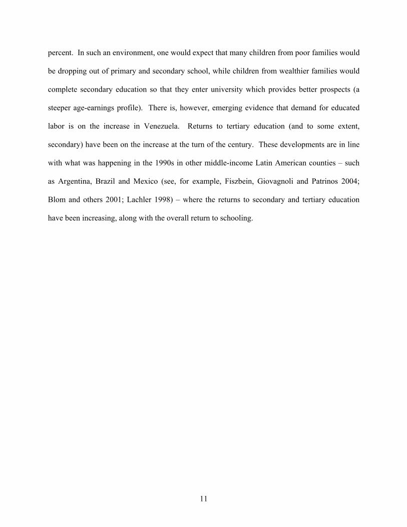
11

percent. In such an environment, one would expect that many children from poor families would

be dropping out of primary and secondary school, while children from wealthier families would

complete secondary education so that they enter university which provides better prospects (a

steeper age-earnings profile). There is, however, emerging evidence that demand for educated

labor is on the increase in Venezuela. Returns to tertiary education (and to some extent,

secondary) have been on the increase at the turn of the century. These developments are in line

with what was happening in the 1990s in other middle-income Latin American counties – such

as Argentina, Brazil and Mexico (see, for example, Fiszbein, Giovagnoli and Patrinos 2004;

Blom and others 2001; Lachler 1998) – where the returns to secondary and tertiary education

have been increasing, along with the overall return to schooling.

12

Table 4: Implied Private Rate of Return to Education per Year, by Level (%): 1992-2000 All Males Females 1992 Primary (vs none) Secondary (vs primary) Higher (vs secondary) University(vs secondary)

16 17 n/a 12

17 15 n/a 12

18 22 n/a 10

1995 Primary (vs none) Secondary (vs primary) Higher (vs secondary) University (vs secondary)

18 16 12 8

18 16 12 8

20 20 11 8

1996 Primary (vs none) Secondary (vs primary) Higher (vs secondary) University(vs secondary)

15 14 13 12

17 14 9

11

16 20 18 11

1997 Primary (vs none) Secondary (vs primary) Higher (vs secondary) University (vs secondary)

16 18 13 11

17 18 13 11

22 23 11 12


16 18 13 10

18 19 13 10

16 21 14 10


17 16 10 10

20 19 9 9

11 22 12 9


15 17 11 8

15 18 10 7

19 18 12 10


15 18 13 11

16 19 14 9

16 20 13 12


17 19 13 13

18 18 13 13

19 22 14 14

Source: Encuesta de Hogares por Muestro

13

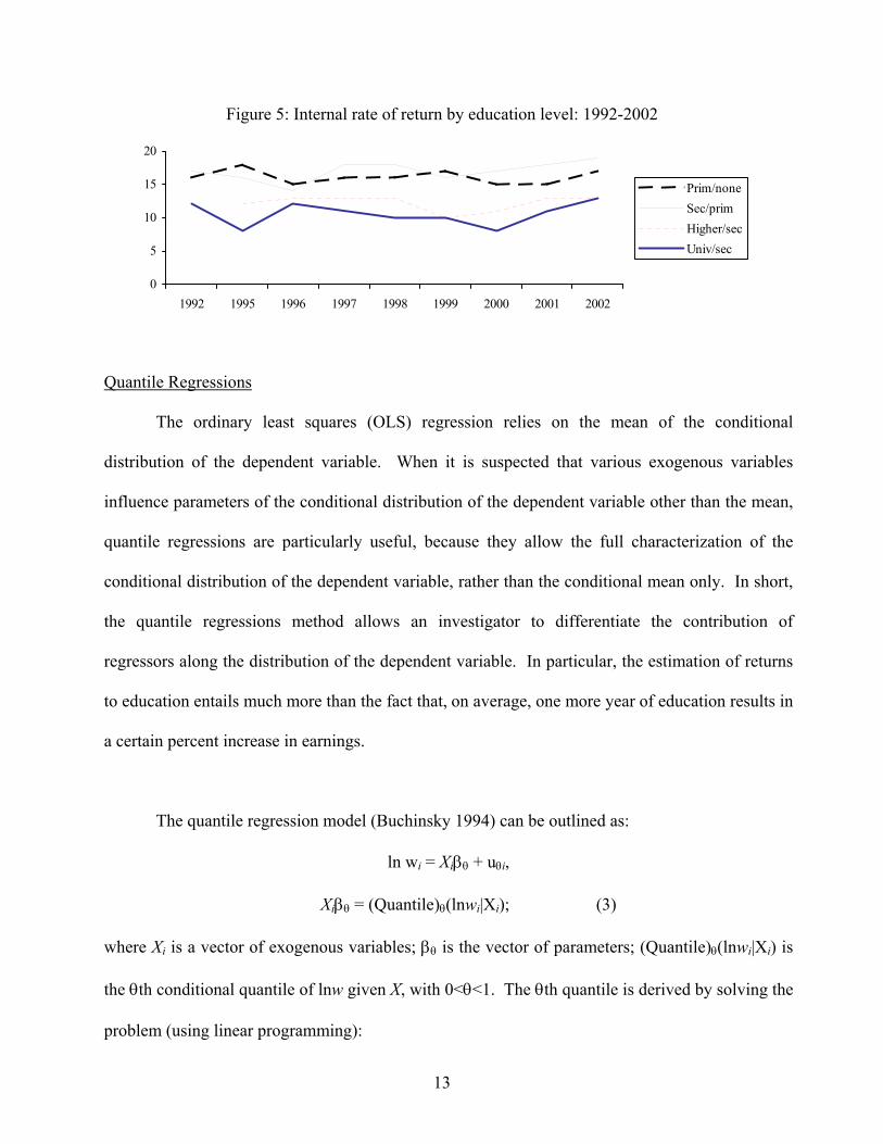
Figure 5: Internal rate of return by education level: 1992-2002

0

5

10

15

20

1992 1995 1996 1997 1998 1999 2000 2001 2002

Prim/noneSec/primHigher/secUniv/sec

Quantile Regressions

The ordinary least squares (OLS) regression relies on the mean of the conditional

distribution of the dependent variable. When it is suspected that various exogenous variables

influence parameters of the conditional distribution of the dependent variable other than the mean,

quantile regressions are particularly useful, because they allow the full characterization of the

conditional distribution of the dependent variable, rather than the conditional mean only. In short,

the quantile regressions method allows an investigator to differentiate the contribution of

regressors along the distribution of the dependent variable. In particular, the estimation of returns

to education entails much more than the fact that, on average, one more year of education results in

a certain percent increase in earnings.

The quantile regression model (Buchinsky 1994) can be outlined as:

ln wi = Xiβθ + uθi,

Xiβθ = (Quantile)θ(lnwi|Xi); (3)

where Xi is a vector of exogenous variables; βθ is the vector of parameters; (Quantile)θ(lnwi|Xi) is

the θth conditional quantile of lnw given X, with 0<θ<1. The θth quantile is derived by solving the

problem (using linear programming):

14

Min Σρθ(lnwi - Xiβθ), (4) β∈Rk i

where ρθ(ε) is the check function defined as ρθ(ε) = θε if ε≥0, and ρθ(ε) = (θ-1)ε if ε<0. Standard

errors are bootstrap standard errors. The median regression is obtained by setting θ = 0.5 and

similarly for other quantiles. As θ is varied from 0 to 1, the entire distribution of the dependent

variable, conditional on X, is traced.

The quantile approach has a number of useful features, in addition to allowing the full

characterization of the conditional distribution of the dependent variable, such as: (a) the linear

programming representation of the quantile regression model makes estimation easy; (b) the

quantile regression objective function is a weighted sum of absolute deviations, resulting in a

robust measure of location, so that the estimated coefficient vector is not sensitive to outlier

observation on the dependent variable; (c) when the error term is non-normal, quantile regression

estimates may be more efficient than OLS estimators (Buchinsky 1998).

Estimated returns to education at different quantiles (0.10, 0.25, 0.50, 0.75 and 0.90) can

provide further insight into within-skill group changes and differences in returns at the upper and

lower level of the income distribution, as well as differences by sex. We find that the

developments in returns over time are sharply different between sexes (Table 5; see also Figures 6

and 7). For all years examined and within each year, male returns exhibit a steady increase as one

goes to higher income quantiles, especially after the 3rd quintile, and the same is true for the return

to labor market experience. Men in higher quantiles of the earnings distribution in Venezuela,

therefore, enjoy higher returns to an additional year of schooling (and experience), compared to

their counterparts at lower quantiles. Looking at the difference in returns across the male earnings

15

distribution over time, we find that the difference in returns between the 90th and the 10th quantile

increases in the post-1995 period compared to the first part of the 1990s. This may mean that the

high earners (at each educational level) are benefiting more over time, compared to the low earners

and that the effect of education upon earnings across the income distribution has become more

acute.

Female returns follow the opposite pattern from that of male returns. Female returns are

highest at the lowest (10th) quantile and steadily decline until the 3rd quantile. For 1992 and 1995

the decline is for the 75th or the 90th quantile. For 1998 and 2000 the decline tapers off or slightly

rebounds by the 50th quantile. Finally, for 2002 returns rebound after the 50th quantile. Possible

reasons for the difference in patterns between men and women in Venezuela could be: (1) there is

significant heterogeneity in the labor market; and (2) discrimination in the labor market against

women limits the earnings potential of the most able.

Increasing returns with quantiles have been observed for a series of countries in Europe –

Portugal, Austria, Finland, Ireland, Netherlands, Norway, Spain, Sweden, Switzerland and the

United Kingdom, while only for Germany and Greece the returns-quantiles profile was found to be

negative. Such international differences provide evidence that the interaction between education

systems and labor market institutions on wage inequality is not identical across countries (Pereira

and Martins 2000). Increasing returns as one goes from the lower to the higher end of the earnings

distribution could be interpreted as an indication of complementarity between ability and education

(or skills), with more able workers benefiting from additional investment in education (see Mwabu

and Schultz 1996 on South Africa). This would be the case of males but not for females in

16

Venezuela. Among males, the increasing quantile returns, besides the aforementioned countries in

Europe, follow the pattern observed for whites in South Africa. Among females, there is no

tendency for the returns to increase with quantiles (with some evidence that quantile returns are

actually decreasing), suggesting that there is no tendency for ability to bias returns upward; this

pattern of quantile returns matches that observed for Africans in South Africa (as well as in

Germany and Greece). However, there are other countries for which education is a substitute for

unobserved ability, including Mexico (Patrinos and Metzger 2004), the Philippines (Sakellariou

2004) and Ethiopia (Girma and Kedir 2004). Also, in a careful analysis of ability and education,

Denny and O’Sullivan (2004) find that education is a substitute for ability in the case of the United

Kingdom. The implication for the case of Venezuela is that education is a good investment that

would help reduce inequality over time.

17

Table 5: Quantile Regressions: Returns to Schooling by Quantile, 1992-2000 (dependent variable: logarithm of monthly earnings)

Males Females 1992 10th quantile 25th quantile 50th quantile 75th quantile 90th quantile

7.2 7.4 7.9 9.1 9.9

13.0 10.7 9.7 10.1 10.8

1995 10th quantile 25th quantile 50th quantile 75th quantile 90th quantile

7.7 8.0 7.6 7.8 9.0

13.8 11.6 9.5 8.4 8.4


7.9 7.7 8.5

10.3 11.5

13.1 11.5 10.9 11.0 11.7


6.9 7.2 7.8 9.0 9.9

11.1 9.6 8.7 9.5 9.9


8.6 8.7 9.0

10.3 11.1

13.4 12.3 12.2 12.6 12.5

Source: Encuesta de Hogares por Muestro; see Annex Table 3

18

Figure 6: Returns to schooling by quintiles, males: 1992-2002

1st 2nd 3rd 4th 5th

Quintile

Ret

urns

1992

1995

1998

2000

2002

Figure 7: Returns to schooling by quintiles, females: 1992-2002

1st 2nd 3rd 4th 5th

Quintile

Ret

urns

19921995199820002002

4. Conclusion

In this paper we have estimated the returns to education in Venezuela for the period

1992-2002 and linked them to earlier available estimates from the 1970s and 1980s. Using

consistent cross-sections from the Encuesta de Hogares por Muestro we documented falling

returns to schooling and educational levels until the mid-1990s, followed by increasing returns

thereafter.

19

The overall return to an additional year of schooling was steadily declining in the 1970s,

1980s and through the mid-1990s. Since then, returns have been exhibiting an increasing trend.

Returns to education by level follow the trend observed in the results on returns to schooling.

Primary and secondary premiums are relatively stable during the decade for both men and

women, while university premiums are more volatile, exhibiting a falling trend from 1996 to

2000 and an increasing trend thereafter. Females, with few exceptions, enjoy higher education

premiums compared to males for all education levels.

The reasons for the observed developments in returns to schooling and education

premiums relate to the effect of the swings in economic activity in Venezuela on the demand and

supply of education and skills. During the 1990s, the Venezuelan economy was characterized by

sharp fluctuations in economic activity, volatile but, overall, decreasing real incomes and a

steady increase in poverty incidence. During the same period, lack of opportunities in the formal

sector resulted in an increasing number of workers moving into the informal sector, where

returns to education are low and poverty is endemic. Lack of sustained dynamism in the

economy leads to a vicious cycle of depressed earnings, falling profitability of investing in

education, and reduced incentive to send children to school (especially given the high incidence

of poverty). At the same time reduced opportunities in the formal sector of the economy result in

those without skills ending up in the informal sector, where wages are low and the poverty

incidence is high, with significant intergenerational problems.

Using quantile regression analysis we find that the developments in returns over time are

sharply different between males and females. For all years examined and within each year, male

20

returns exhibit a steady increase as one goes to higher income quantiles. Men in higher quantiles

of the earnings distribution in Venezuela, enjoy higher returns to an additional year of schooling

(and experience), compared to their counterparts at lower quantiles. Female returns follow the

opposite pattern from that of male returns. They are highest at the lowest (10th) quantile and

decline thereafter. Increasing returns as one goes from the lower to the higher end of the earnings

distribution could be interpreted as an indication of complementarity between ability and education

(or skills), with more able workers benefiting from additional investment in education. In

Venezuela, this would be the case of males but not for females. For females, education is a good

investment that allows those less well endowed with ability to increase their earnings.

We also find that the difference in returns between the high and low earners increases in

the post-1995 period compared to the first part of the 1990s. This may mean that the high earners

(at each educational level) are benefiting more, over time, compared to the low earners and that the

effect of education upon earnings across the income distribution has become more acute.

21

References Asplund, R. and P. T. Pereira (Eds.). 1999. Returns to Human Capital in Europe: A Literature

Review, ETLA, Helsinki. Blom, A., L. Holm-Nielsen and D. Verner. 2001. “Education, Earnings and Inequality in Brazil,

1982-98: Implications for Education Policy.” World Bank Policy Research Working Paper 2686, Washington D.C.

Buchinsky, M. 1994. “Changes in the U.S. Wage Structure 1963-1987: An Application of

Quantile Regression.” Econometrica 62 (March): 405-58. Buchinsky, M. 1998. “Recent Advances in Quantile Regression Models.” Journal of Human

Resources 33 (Fall): 88-126. Denny, K. and V. O’Sullivan. 2004. “Can Education Compensate for Low Ability? Evidence

from British Data.” Institute for Fiscal Studies WP04/19. Fersterer J. and R. Winter-Ebmer. 2003. “Are Austrian Returns to Education Falling Over

Time?” Labour Economics 10: 73-89. Fiszbein, A. and G. Psacharopoulos. 1993. “A Cost-Benefit Analysis of Educational Investment

in Venezuela: 1989 Update.” Economics of Education Review 12 (4): 293-298. Fiszbein, A., P.I. Giovagnoli and H.A. Patrinos. 2004. “Estimating the Returns to Education in

Argentina: 1992-2002.” Washington, DC: World Bank (processed). Girma, S. and A. Kedir. 2003. "Is Education More Benficial to the Less Able? Eocnometric

Evidence from Ethiopia." Discussion Papers in Economics from Department of Economics No 03/1, University of Leicester.

Harmon, C., I. Walker and Westergaard-Nielsen (Eds.). 2001. Education and Earnings in

Europe: A Cross-Country Analysis of the Returns to Education. Edward Elgar, Cheltenham.

Lachler, U. 1998. “Education and Earnings Inequality in Mexico.” World Bank Policy Research

Working Paper 1949, Washington, D.C. Mincer, J. 1974. Schooling Experience and Earnings. Columbia University Press, New York. Mosconi G. M. and C. Alvarez. 1996. “Poverty and the Labor Market in Venezuela: 1982-1995.”

No SOC96-101, Washington, D.C. (December). Mwabu, G. and P. T. Schultz. 1996. “Education Returns Across Quantiles of the Wage Function:

Alternative Explanations for Returns to Education by Race in South Africa. American Economic Review Papers and Proceedings 86: 335-339.

22

Patrinos, H.A. and S. Metzger. 2004. "Returns to Education in Mexico: An Update." World Bank/UDLA (processed).

Pereira, P. T. and P. S. Martins. 2000. “Does Education Reduce Wage Inequality? Quantile

Regressions Evidence from Fifteen European Countries.” IZA Discussion Paper N0. 120 (February).

Psacharopoulos, G. and A. Alam. 1991. “Earnings and Education in Venezuela: An Update form

the 1987 Household Survey.” Economics of Education Review 10 (1): 29-36. Psacharopoulos, G. and H.A. Patrinos. 2004. “Returns to Investment in Education: A Further

Update.” Education Economics 12(2): forthcoming. Psacharopoulos G. and F. Steier. 1988. “Education and the Labor Market in Venezuela: 1975-

1984.” Economics of Education Review 7 (3): 321-332. Sakellariou, C. 2004. "The use of quantile regressions in estimating gender wage differentials: a

case study of the Philippines." Applied Economics 36(9): 1001-1007.

23

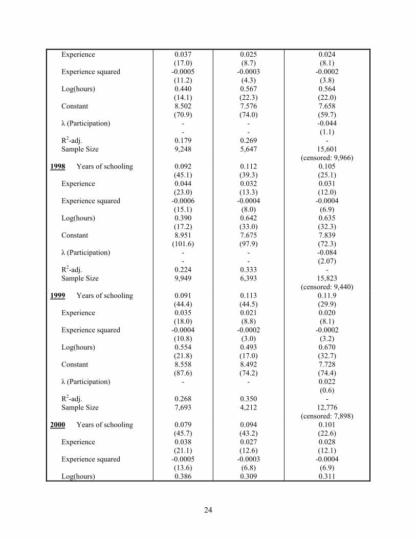
Annex Table 1: Mincer Equations (by Sex): 1992-2000 (Dep. Variable: Logarithm of Monthly Earnings) Variable Males Females without

Sample Selection Females with

Sample Selection 1992 Years of schooling Experience Experience squared Log(hours) Constant λ (Participation) R2-adj. Sample Size

0.084 (128.8) 0.037 (56.5)

-0.0005 (36.9) 0.550 (38.1) 3.987 (72.6)

- -

0.335 41,341

0.110 (113.1) 0.031 (33.6)

-0.0004 (18.8) 0.254 (15.3) 4.640 (70.7)

- -

0.380 22,769

0.11.9 (95.5) 0.029 (31.0)

-0.0003 (16.4) 0.523 (45.0) 3.488 (70.5) 0.097 (8.8)

- 59,827

(censored: 35,463) 1995 Years of schooling Experience Experience squared Log(hours) Constant λ (Participation) R2-adj. Sample Size

0.080 (43.8) 0.036 (21.5)

-0.0005 (14.1) 0.419 (18.1) 7.607 (83.0)

- -

0.196 10,843

0.099 (39.5) 0.026 (11.2)

-0.0003 (5.3) 0.377 (12.2) 7.466 (61.5)

- -

0.228 5,817

0.096 (24.6) 0.021 (7.9)

-0.0002 (3.9) 0.591 (25.5) 6.792 (56.6) -0.043 (1.5)

- 17,652


0.074 (34.4) 0.038 (18.1)

-0.0005 (13.0) 0.396 (14.6) 8.229 (78.3)

- -

0.158 9,312

0.103 (36.9) 0.026 (10.0)

-0.0003 (6.1) 0.562 (24.6) 7.137 (77.9)

- -

0.279 5,885

0.101 (27.9) 0.025 (9.5)

-0.0003 (5.7) 0.560 (24.3) 7.174 (64.8) -0.019 (0.6)

- 15,579

(censored: 9,699) 1997 Years of schooling

0.091 (39.0)

0.120 (36.4)

0.117 (27.3)

24

Experience Experience squared Log(hours) Constant λ (Participation) R2-adj. Sample Size

0.037 (17.0)

-0.0005 (11.2) 0.440 (14.1) 8.502 (70.9)

- -

0.179 9,248

0.025 (8.7)

-0.0003 (4.3) 0.567 (22.3) 7.576 (74.0)

- -

0.269 5,647

0.024 (8.1)

-0.0002 (3.8) 0.564 (22.0) 7.658 (59.7) -0.044 (1.1)

- 15,601


0.092 (45.1) 0.044 (23.0)

-0.0006 (15.1) 0.390 (17.2) 8.951

(101.6) - -

0.224 9,949

0.112 (39.3) 0.032 (13.3)

-0.0004 (8.0) 0.642 (33.0) 7.675 (97.9)

- -

0.333 6,393

0.105 (25.1) 0.031 (12.0)

-0.0004 (6.9) 0.635 (32.3) 7.839 (72.3) -0.084 (2.07)

- 15,823


0.091 (44.4) 0.035 (18.0)

-0.0004 (10.8) 0.554 (21.8) 8.558 (87.6)

-

0.268 7,693

0.113 (44.5) 0.021 (8.8)

-0.0002 (3.0) 0.493 (17.0) 8.492 (74.2)

-

0.350 4,212

0.11.9 (29.9) 0.020 (8.1)

-0.0002 (3.2) 0.670 (32.7) 7.728 (74.4) 0.022 (0.6)

- 12,776

(censored: 7,898) 2000 Years of schooling Experience Experience squared Log(hours)

0.079 (45.7) 0.038 (21.1)

-0.0005 (13.6) 0.386

0.094 (43.2) 0.027 (12.6)

-0.0003 (6.8) 0.309

0.101 (22.6) 0.028 (12.1)

-0.0004 (6.9) 0.311

25

Constant λ (Participation) R2-adj. Sample Size

(20.7) 9.408

(128.9) - -

0.244 9,383

(14.7) 9.502

(112.8) - -

0.296 5,315

(14.7) 9.349 (77.0) 0.078 (1.7)

- 14,229


0.091 (51.5) 0.039 (22.0)

-0.0005 (13.5) 0.423 (25.0) 9.248

(140.1) -

0.340 7,786

0.113 (51.1) 0.025 (11.4)

-0.0002 (4.3) 0.347 (16.8) 9.265

(111.6) -

0.406 4,388

0.118 (28.8) 0.025 (10.7)

-0.0002 (5.1) 0.653 (40.0) 8.097 (81.6) -0.044 (0.9)

- 12,358

(censored: 7,400)

2002 Years of schooling Experience Experience squared Log(hours) Constant λ (Participation) R2-adj. Sample Size

0.099 (54.0) 0.045 (24.7)

-0.0006 (17.2) 0.487 (27.9) 9.016

(131.7) -

0.366 7,720

0.127 (54.7) 0.033 (14.1)

-0.0004 (7.0) 0.581 (28.4) 8.299

(100.9) -

0.457 4,735

0.132 (32.8) 0.032 (12.9)

-0.0004 (6.9) 0.756 (45.1) 7.604 (77.4) 0.005 (0.1)

- 12,609

(censored: 7,325) Source: Encuesta de Hogares por Muestro Note: t-values in parentheses (z-values for selection equation). Determinants of the selection equation are: years of education, age, age squared, marital status and number of children in the household.

26

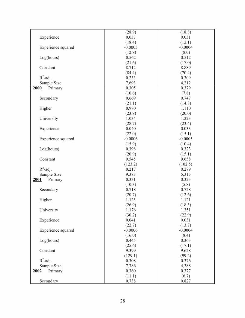
Annex Table 2: Earnings Premium by Level of Education (by Sex): 1992-2000 (Dependent Variable: Logarithm of Monthly Earnings)

Variable Males Females 1992 Primary Secondary Higher University Experience Experience squared Log(hours) Constant R2-adj. Sample Size

0.347 (28.8) 0.657 (53.2)

n/a

1.281 (93.0) 0.040 (59.7)

-0.0006 (41.1) 0.569 (39.0) 3.987 (71.2) 0.329

41,039

0.370 (15.7) 0.879 (36.4)

n/a

1.492 (59.2) 0.036 (37.4)

-0.0005 (23.3) 0.211 (12.3) 4.945 (71.3) 0.352

22,663 1995 Primary Secondary Higher University Experience Experience squared Log(hours) Constant R2-adj. Sample Size

0.365 (12.2) 0.695 (21.3) 1.057 (23.8) 1.107 (28.4) 0.037 (21.8)

-0.0005 (16.1) 0.444 (18.5) 7.701 (80.6) 0.175

11,000

0.402 (7.8) 0.811 (15.0) 1.144 (17.9) 1.228 (21.4) 0.031 (13.0)

-0.0005 (8.6) 0.382 (12.1) 7.679 (59.2) 0.198 5881

1996 Primary Secondary Higher University Experience Experience squared

0.337 (9.0) 0.627 (15.4) 0.892 (11.7) 1.184 (20.1) 0.038 (17.6)

-0.0006

0.324 (5.1) 0.731 (11.0) 1.267 (14.4) 1.399 (18.2) 0.031 (10.6)

-0.0005

27

Log(hours) Constant R2-adj. Sample Size

(14.0) 0.455 (16.6) 8.155 (74.2) 0.130 8,534

(7.9) 0.376 (11.1) 8.194 (57.7) 0.197 4,441

1997 Primary Secondary Higher University Experience Experience squared Log(hours) Constant R2-adj. Sample Size

0.341 (9.6) 0.717 (18.3) 1.103 (20.6) 1.277 (26.2) 0.039 (17.8)

-0.0006 (13.4) 0.537 (17.9) 8.357 (70.2) 0.168 9,283

0.450 (7.0) 0.914 (13.7) 1.232 (16.0) 1.508 (21.1) 0.034 (11.6)

-0.0005 (8.1) 0.290 (8.5) 8.915 (61.9) 0.209 5,082


0.376 (10.9) 0.767 (20.4) 1.169 (24.6) 1.261 (30.1) 0.045 (22.9)

-0.0007 (16.7) 0.375 (15.3) 9.218 (93.5) 0.210 9,828

0.327 (4.6) 0.759 (10.4) 1.184 (15.2) 1.269 (17.1) 0.036 (13.9)

-0.0005 (9.5) 0.507 (15.8) 8.607 (61.2) 0.245 5,494

1999 Primary Secondary Higher University

0.399 (11.6) 0.780 (20.8) 1.045 (21.6) 1.255

0.228 (3.8) 0.667 (10.6) 1.022 (14.9) 1.222

28

Experience Experience squared Log(hours) Constant R2-adj. Sample Size

(28.9) 0.037 (18.4)

-0.0005 (12.8) 0.562 (21.6) 8.712 (84.4) 0.233 7,693

(18.8) 0.031 (12.1)

-0.0004 (8.0) 0.512 (17.0) 8.889 (70.4) 0.309 4,212


0.305 (10.6) 0.669 (21.1) 0.980 (23.8) 1.034 (28.7) 0.040 (22.0)

-0.0006 (15.9) 0.398 (20.9) 9.545

(123.2) 0.217 9,383

0.379 (7.8) 0.747 (14.8) 1.110 (20.0) 1.223 (23.4) 0.033 (15.1)

-0.0005 (10.4) 0.323 (15.1) 9.658

(102.5) 0.279 5,315


0.331 (10.3) 0.718 (20.7) 1.125 (26.9) 1.176 (30.2) 0.041 (22.7)

-0.0006 (16.0) 0.445 (25.6) 9.399

(129.1) 0.308 7,786

0.323 (5.8) 0.728 (12.6) 1.121 (18.3) 1.351 (22.9) 0.031 (13.7)

-0.0004 (8.4) 0.363 (17.1) 9.628 (99.2) 0.376 4,388

2002 Primary Secondary

0.360 (11.1) 0.738

0.377 (6.7) 0.827

29

Higher University Experience Experience squared Log(hours) Constant R2-adj. Sample Size

(21.0) 1.122 (26.2) 1.389 (35.4) 0.047 (24.8)

-0.0007 (19.4) 0.516 (29.0) 9.192

(124.0) 0.343 7,720

(14.1) 1.241 (19.8) 1.550 (25.8) 0.041 (16.6)

-0.0006 (11.5) 0.599 (28.3) 8.689 (89.7) 0.424 (4,735

Source: Encuesta de Hogares por Muestro Note: t-values in parentheses

30

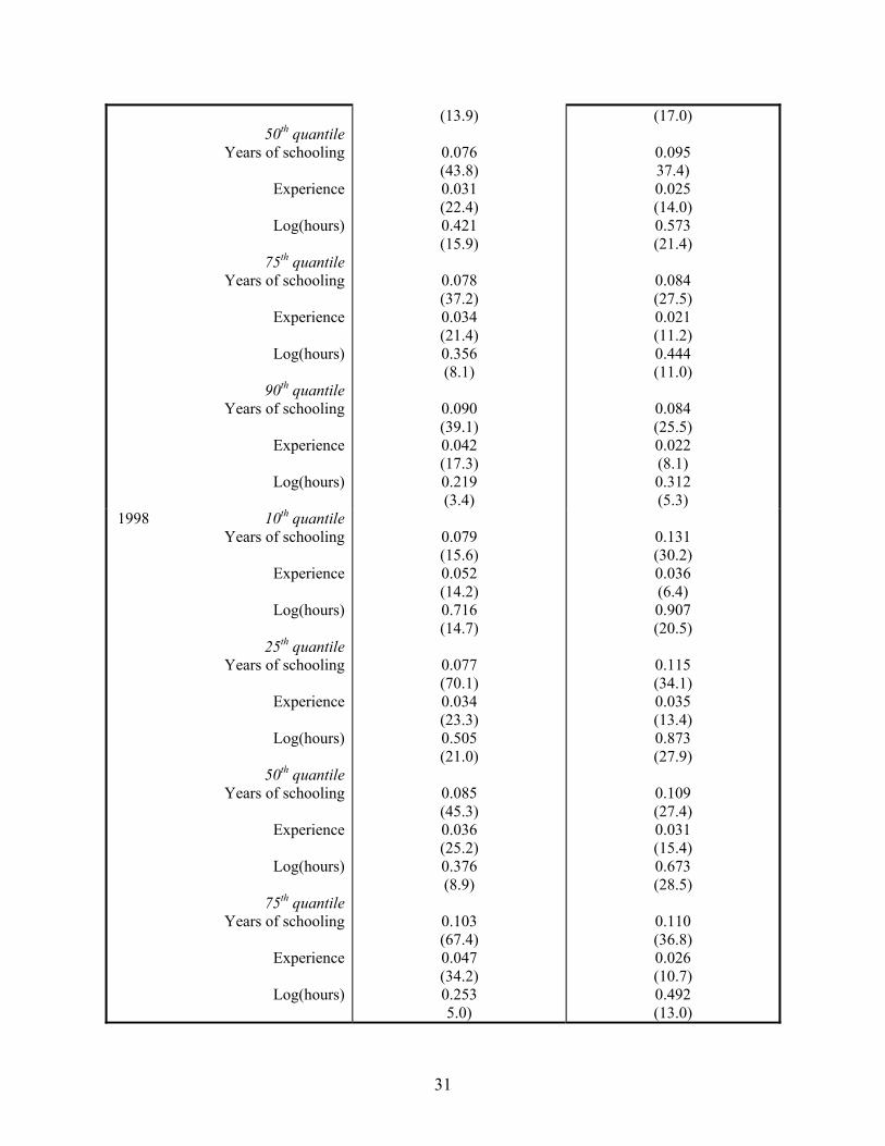
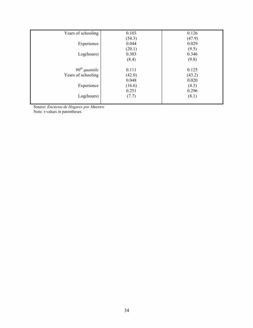
Annex Table 3: Quantile Regressions Returns to Schooling, 1992-2000 (Dep Var: Log Monthly Earnings) Variable Males Females 1992 10th quantile

Years of schooling

Experience

Log(hours)

25th quantile Years of schooling

Experience

Log(hours)

50th quantile

Years of schooling

Experience

Log(hours)


Experience

Log(hours)

90th quantile

Years of schooling

Experience

Log(hours)

0.072 (49.6) 0.037 (36.6) 0.648 (15.1)

0.074 (75.5) 0.036 (40.2) 0.450 (16.6)

0.079

(128.7) 0.036 (64.9) 0.446 (29.0)

0.091

(105.3) 0.039 (47.2) 0.413 (21.6)

0.099 (72.4) 0.042 (29.4) 0.493 (18.2)

0.130 (59.8) 0.036 (16.3) 0.300 (11.7)

0.107 (61.4) 0.029 (27.7) 0.214 (10.3)

0.097 (87.0) 0.027 (29.3) 0.125 (9.7)

0.101

(107.0) 0.030 (26.1) 0.244 (9.6)

0.108 (74.9) 0.032 (18.9) 0.388 (16.6)

1995 10th quantile Years of schooling

Experience

Log(hours)

25th quantile

Years of schooling

Experience

Log(hours)

0.077 (22.7) 0.036 (12.8) 0.486 (9.3)

0.080 (47.2) 0.035 (15.2) 0.468

0.138 (33.2) 0.022 (6.0) 0.727 (12.1)

0.116 (55.3) 0.028 (13.5) 0.697

31

50th quantile

Years of schooling

Experience

Log(hours)


Experience

Log(hours)

90th quantile

Years of schooling

Experience

Log(hours)

(13.9)

0.076 (43.8) 0.031 (22.4) 0.421 (15.9)

0.078 (37.2) 0.034 (21.4) 0.356 (8.1)

0.090 (39.1) 0.042 (17.3) 0.219 (3.4)

(17.0)

0.095 37.4) 0.025 (14.0) 0.573 (21.4)

0.084 (27.5) 0.021 (11.2) 0.444 (11.0)

0.084 (25.5) 0.022 (8.1) 0.312 (5.3)


Experience

Log(hours)

25th quantile

Years of schooling

Experience

Log(hours)


Experience

Log(hours)

75th quantile

Years of schooling

Experience

Log(hours)

0.079 (15.6) 0.052 (14.2) 0.716 (14.7)

0.077 (70.1) 0.034 (23.3) 0.505 (21.0)

0.085 (45.3) 0.036 (25.2) 0.376 (8.9)

0.103 (67.4) 0.047 (34.2) 0.253 5.0)

0.131 (30.2) 0.036 (6.4) 0.907 (20.5)

0.115 (34.1) 0.035 (13.4) 0.873 (27.9)

0.109 (27.4) 0.031 (15.4) 0.673 (28.5)

0.110 (36.8) 0.026 (10.7) 0.492 (13.0)

32


Experience

Log(hours)

0.115 (36.6) 0.057 (19.1) 0.216 (3.0)

0.117 (23.0) 0.035 (10.3) 0.292 (7.2)


Experience

Log(hours)

25th quantile

Years of schooling

Experience

Log(hours)


Experience

Log(hours)

75th quantile

Years of schooling

Experience

Log(hours)


Experience

Log(hours)

0.069 (26.4) 0.038 (10.9) 0.691 (16.9)

0.072 (44.5) 0.031 (16.0) 0.504 (37.0)

0.078 (45.9) 0.032 (38.5) 0.374 (11.5)

0.090 (43.8) 0.043 (35.3) 0.192 (6.6)

0.099 (64.2) 0.051 (19.0) 0.160 (7.0)

0.111 (31.5) 0.038 (6.0) 0.562 (10.2)

0.096 (36.7) 0.029 (10.8) 0.425 (14.4)

0.087 (33.8) 0.022 (8.7) 0.244 (7.0)

0.095 (34.4) 0.020 (5.7) 0.146 (3.1)

0.099 (26.3) 0.017 (4.3) 0.107 (4.7)

2001 10th quintile Years of schooling

Experience

Log(hours)

0.071 (21.2) 0.037 (10.3) 0.642 (21.6)

0.115 (24.8) 0.029 (5.2) 0.542 (9.9)

33


Experience

Log(hours)

50th quantile

Years of schooling

Experience

Log(hours)


Experience

Log(hours)

90th quantile

Years of schooling

Experience

Log(hours)

0.073 (26.2) 0.032 (13.7) 0.481 (15.7)

0.083 (53.0) 0.031 (21.7) 0.364 (18.6)

0.102 (50.5) 0.040 (19.2) 0.308 (14.5)

0.109 (42.2) 0.048 (13.4) 0.243 (5.7)

0.103 (24.7) 0.027 (8.0) 0.394 (10.9)

0.105 (35.4) 0.023 (10.7) 0.269 (9.0)

0.115 (35.2) 0.022 (7.6) 0.206 (6.2)

0.122 (38.6) 0.023 (6.7) 0.211 (5.3)

2002 10th quintile Years of schooling

Experience

Log(hours)

25th quantile

Years of schooling

Experience

Log(hours)


Experience

Log(hours)

75th quantile

0.087 (27.1) 0.050 (11.7) 0.754 (22.1)

0.087 (31.1) 0.039 (17.7) 0.539 (18.3)

0.090 (41.1) 0.038 (20.3) 0.390 (14.3)

0.134 (26.8) 0.038 (6.5) 0.807 (14.0)

0.123 (30.8) 0.039 (11.7) 0.645 (15.2)

0.122 (40.4) 0.031 (12.4) 0.478 (17.4)

34

Years of schooling

Experience

Log(hours)


Experience

Log(hours)

0.103 (54.3) 0.044 (20.1) 0.303 (8.4)

0.111 (42.0) 0.048 (16.6) 0.251 (7.7)

0.126 (47.9) 0.029 (9.5) 0.346 (9.8)

0.125 (43.2) 0.020 (4.3) 0.296 (8.1)

Source: Encuesta de Hogares por Muestro Note: t-values in parentheses

economic volatility and returns to education in venezuela

Documents