econ-115 lecture 10 midterm review...midterm review industrial organization 1. bertrand model of...
TRANSCRIPT

ECON/MGMT 115
Industrial Organization
MIDTERM REVIEW

Industrial Organization
1. Bertrand Model of Oligopoly
2. Cournot & Bertrand
3
Industrial Organization
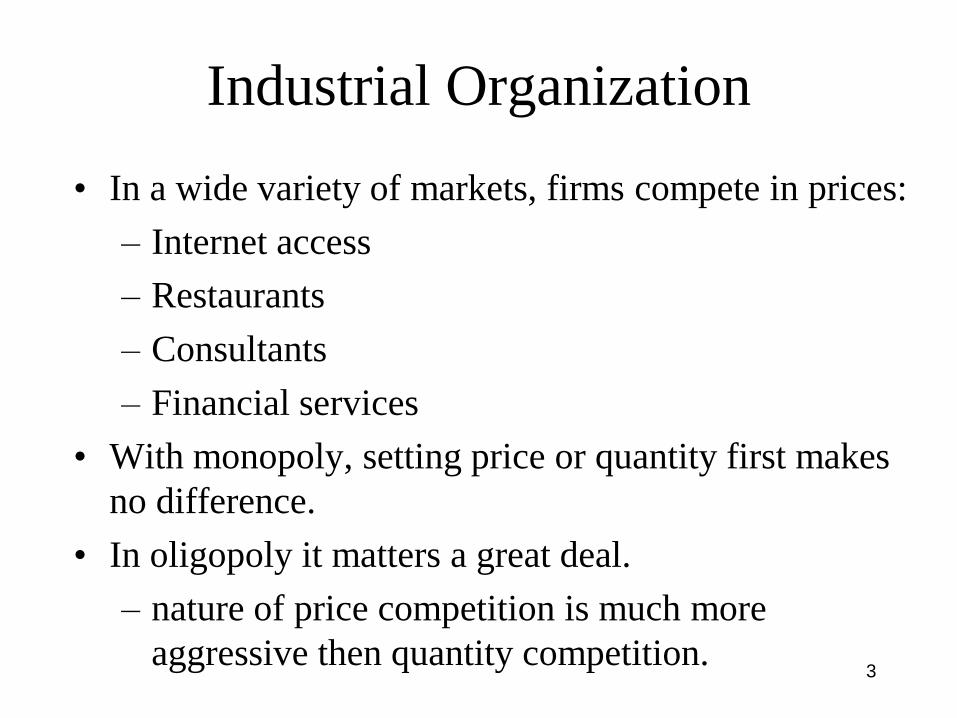
• In a wide variety of markets, firms compete in prices:
– Internet access
– Restaurants
– Consultants
– Financial services
• With monopoly, setting price or quantity first makes
no difference.
• In oligopoly it matters a great deal.
– nature of price competition is much more
aggressive then quantity competition.
4
Industrial Organization
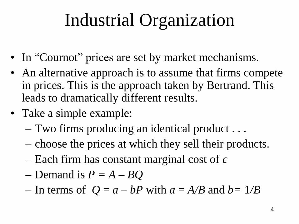
• In “Cournot” prices are set by market mechanisms.
• An alternative approach is to assume that firms compete in prices. This is the approach taken by Bertrand. This leads to dramatically different results.
• Take a simple example:
– Two firms producing an identical product . . .
– choose the prices at which they sell their products.
– Each firm has constant marginal cost of c
– Demand is P = A – BQ
– In terms of Q = a – bP with a = A/B and b= 1/B
5
Industrial Organization
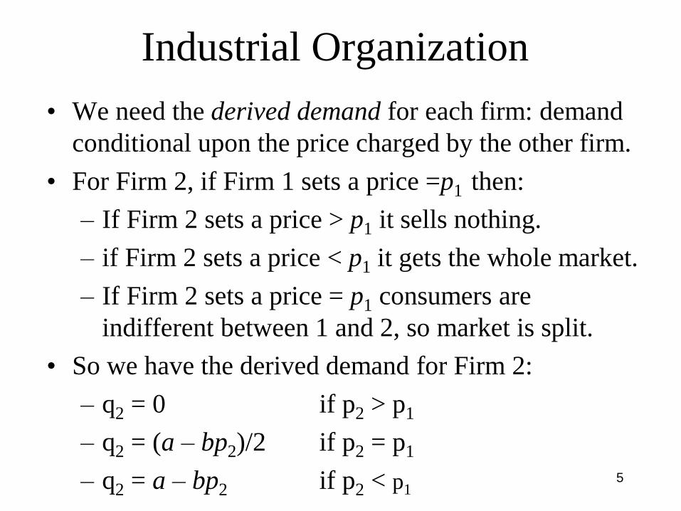
• We need the derived demand for each firm: demand
conditional upon the price charged by the other firm.
• For Firm 2, if Firm 1 sets a price =p1 then:
– If Firm 2 sets a price > p1 it sells nothing.
– if Firm 2 sets a price < p1 it gets the whole market.
– If Firm 2 sets a price = p1 consumers are
indifferent between 1 and 2, so market is split.
• So we have the derived demand for Firm 2:
– q2 = 0 if p2 > p1
– q2 = (a – bp2)/2 if p2 = p1
– q2 = a – bp2 if p2 < p1

6
Industrial Organization
• This can be illustrated
by the graph to the
right.
– Demand is
discontinuous.
– The discontinuity
in demand carries
over to profit.
p2
q2
p1
aa - bp1(a - bp1)/2
There is a
jump at p2 = p1

7
Industrial Organization
Firm 2’s profit is:
p2(p1,, p2) = 0 if p2 > p1
p2(p1,, p2) = (p2 - c)(a - bp2) if p2 < p1
p2(p1,, p2) = (p2 - c)(a - bp2)/2 if p2 = p1
Clearly this depends on p1.
Now suppose Firm 1 sets a “very high” price:
greater than the monopoly price of pM = (a
+c)/2b
For whatever
reason!

8
Industrial Organization
With p1 > (a + c)/2b, Firm 2’s profit looks like this:
Firm 2’s Price
Firm 2’s Profit
c (a+c)/2
b
p1
p2 < p1
p2 = p1
p2 > p1
9
Industrial Organization
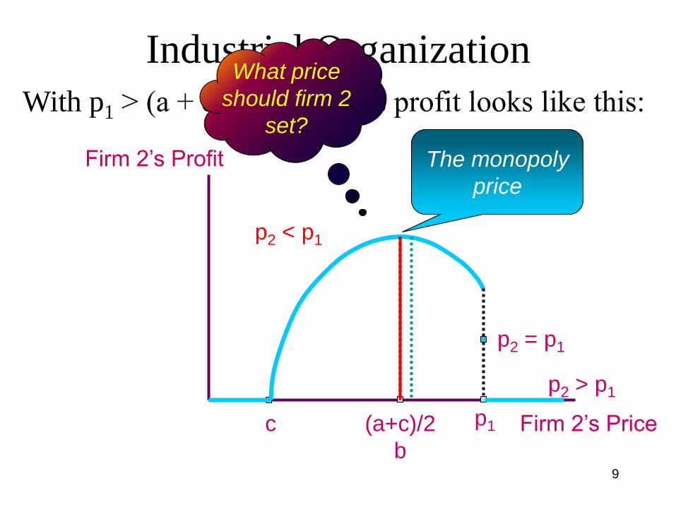
With p1 > (a + c)/2b, Firm 2’s profit looks like this:
Firm 2’s Price
Firm 2’s Profit
c (a+c)/2
b
p1
p2 < p1
p2 = p1
p2 > p1
What price
should firm 2
set?
The monopoly
price
10
Industrial Organization
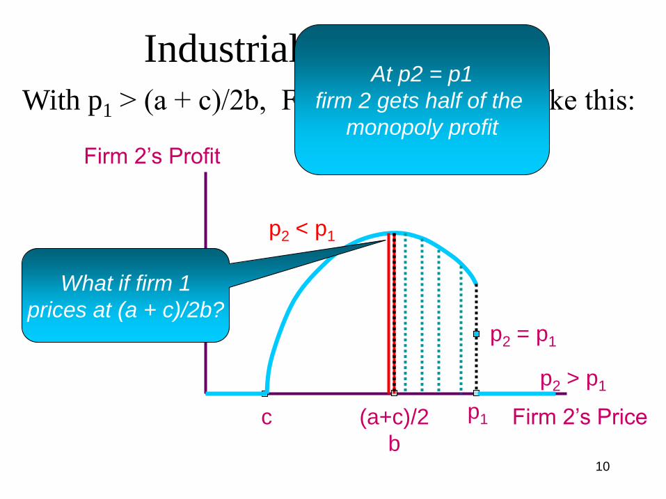
With p1 > (a + c)/2b, Firm 2’s profit looks like this:
Firm 2’s Price
Firm 2’s Profit
c (a+c)/2
b
p1
p2 < p1
p2 = p1
p2 > p1
What if firm 1
prices at (a + c)/2b?
At p2 = p1
firm 2 gets half of the
monopoly profit

11
Industrial Organization
With p1 > (a + c)/2b, Firm 2’s profit looks like this:
Firm 2’s Price
Firm 2’s Profit
c (a+c)/2
b
p1
p2 < p1
p2 = p1
p2 > p1
So firm 2 should just
undercut p1 a bit and
get almost all the
monopoly profit
Firm 2 will only earn a
positive profit by cutting its
price to (a + c)/2b or less

12
Industrial Organization
Now suppose Firm 1 sets a price less than (a + c)/2b
Firm 2’s Price
Firm 2’s Profit
c (a+c)/2
b
p1
p2 < p1
p2 = p1
p2 > p1
Firm 2’s profit looks like this: What price
should firm 2
set now?
As long as p1 > c,
Firm 2 should aim just
to undercut firm 1
Of course, firm 1
will then undercut
firm 2 and so on

13
Industrial Organization
Now suppose Firm 1 sets a price less than (a + c)/2b
Firm 2’s Price
Firm 2’s Profit
c (a+c)/2
b
p1
p2 <
p1
p2 = p1
p2 > p1
Firm 2’s profit looks like this:
What if firm 1
prices at c?
Then firm 2 should also price
at c. Cutting price below cost
gains the whole market but loses
money on every customer
14
Industrial Organization
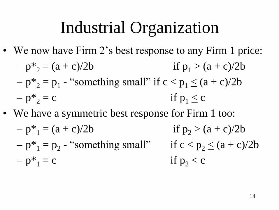
• We now have Firm 2’s best response to any Firm 1 price:
– p*2 = (a + c)/2b if p1 > (a + c)/2b
– p*2 = p1 - “something small” if c < p1 < (a + c)/2b
– p*2 = c if p1 < c
• We have a symmetric best response for Firm 1 too:
– p*1 = (a + c)/2b if p2 > (a + c)/2b
– p*1 = p2 - “something small” if c < p2 < (a + c)/2b
– p*1 = c if p2 < c
15
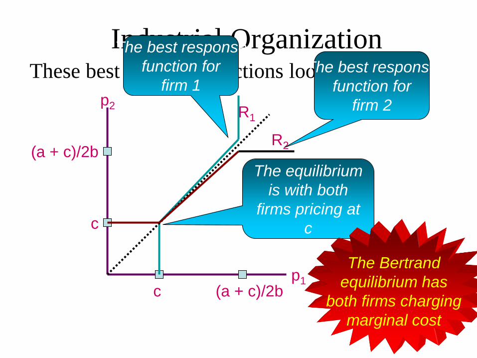
Industrial OrganizationThese best response functions look like this:
p2
p1c
c
R1
R2
The best response
function for
firm 1The best response
function for
firm 2
The equilibrium
is with both
firms pricing at
c
The Bertrand
equilibrium has
both firms charging
marginal cost
(a + c)/2b
(a + c)/2b

16
Industrial Organization
• The Bertrand model makes clear that competing on
price is very different from competition in quantities.
COURNOT: Pmonopoly > Pcournot > Pcompetitive
BERTRAND: Pmonopoly > Pbertrand = Pcompetitive
• Since many firms seem to set prices (not quantities),
this is a challenge to the Cournot approach.
• But is this positive outcome likely? We will now
consider two extensions of the Bertrand model that
will provide a more nuanced approach to oligopolies:
– the impact of capacity constraints; and
– product differentiation

17
Industrial Organization
• p = c equilibrium requires both firms have sufficient capacity to meet all demand at p = c
• However, if there is insufficient capacity, capacity constraints may affect the equilibrium.
• Consider an example:
– daily demand for skiing is Q = 6,000 – 60P
• Q is number of lift tickets; P is the ticket price.
– Two resorts: Pepall and Richards have fixed daily capacities: Pepall = 1,000 and Richards =1,400.
– marginal cost of lift services for both is $10.

18
Industrial Organization
• Is a price P = c = $10 a Nash equilibrium?
– total demand is 5,400 > 2,400 capacity.
– Assume Firm 1 sets its price at c.
– From Firm 2’s perspective:
• At p = c there is insufficient capacity to
serve the entire market.
• Why not set p2 > c?
• Firm 2 loses some customers. But it retains
others, from whom it now earns a profit.
• Therefore, P = c = $10 is not a Nash equilibrium.

19
Industrial Organization• Assume that at any price where demand at a resort
is greater than capacity there is efficient rationing.
– serves skiers with the highest willingness to pay
• Then we can derive residual demand:
• If P = $60, total demand = 2,400 = total capacity.
– Pepall gets 1,000 skiers.
– Residual demand to Richards with efficient
rationing is Q = 5000 – 60P or P = 83.33 –
Q/60 in inverse form.
– marginal revenue is then MR = 83.33 – Q/30
20
Industrial Organization
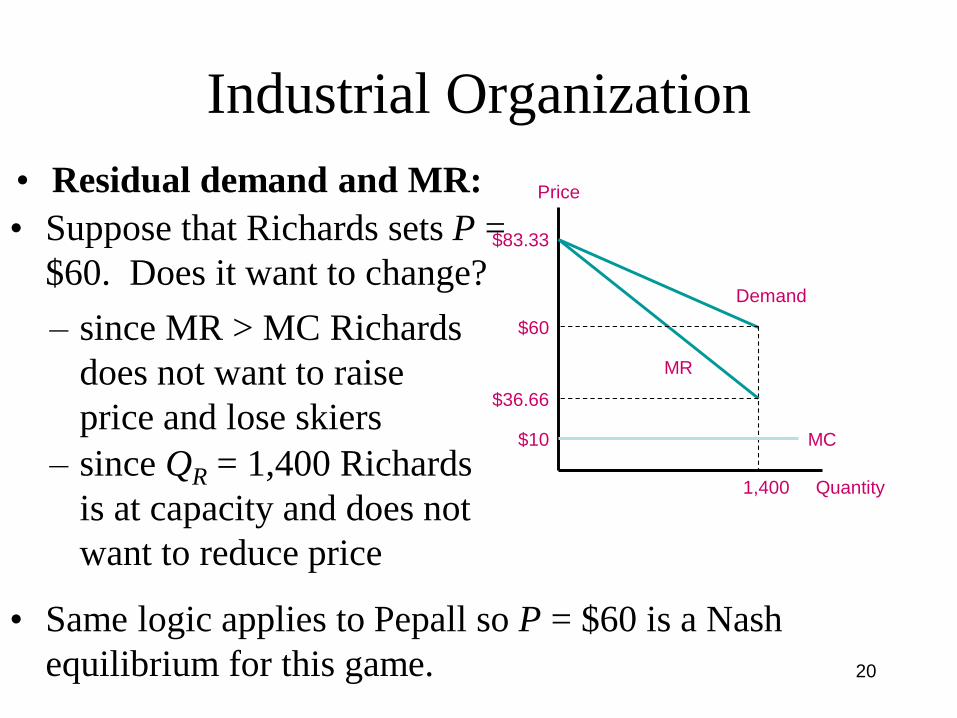
• Residual demand and MR: Price
Quantity
Demand
1,400
$83.33
$60
$36.66
$10 MC
MR
• Suppose that Richards sets P =
$60. Does it want to change?
– since MR > MC Richards
does not want to raise
price and lose skiers
– since QR = 1,400 Richards
is at capacity and does not
want to reduce price
• Same logic applies to Pepall so P = $60 is a Nash
equilibrium for this game.
21
Industrial Organization
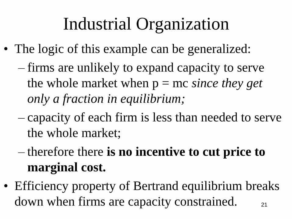
• The logic of this example can be generalized:
– firms are unlikely to expand capacity to serve
the whole market when p = mc since they get
only a fraction in equilibrium;
– capacity of each firm is less than needed to serve
the whole market;
– therefore there is no incentive to cut price to
marginal cost.
• Efficiency property of Bertrand equilibrium breaks
down when firms are capacity constrained.
22
Industrial Organization
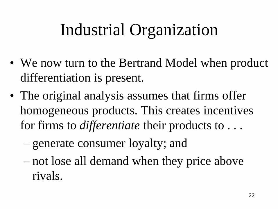
• We now turn to the Bertrand Model when product
differentiation is present.
• The original analysis assumes that firms offer
homogeneous products. This creates incentives
for firms to differentiate their products to . . .
– generate consumer loyalty; and
– not lose all demand when they price above
rivals.
23
Industrial Organization
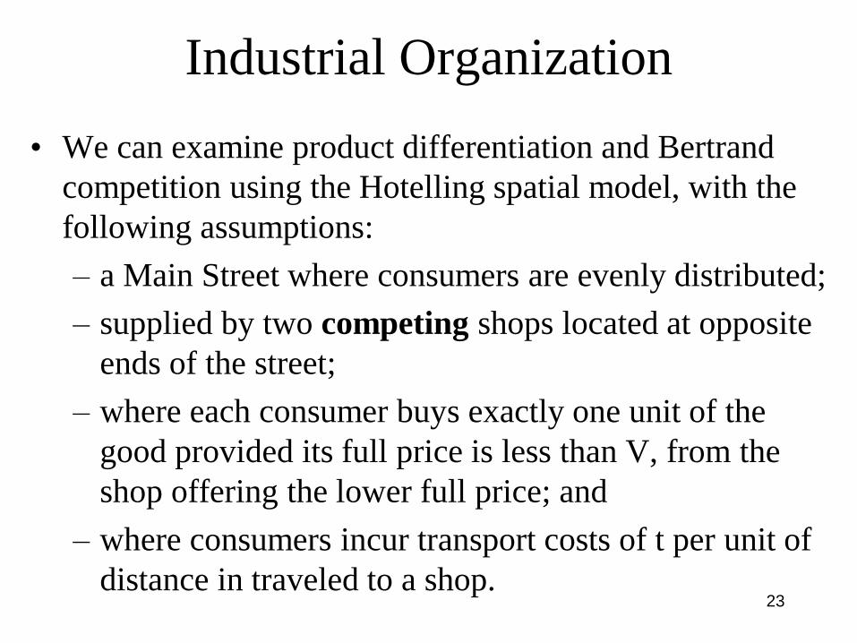
• We can examine product differentiation and Bertrand
competition using the Hotelling spatial model, with the
following assumptions:
– a Main Street where consumers are evenly distributed;
– supplied by two competing shops located at opposite
ends of the street;
– where each consumer buys exactly one unit of the
good provided its full price is less than V, from the
shop offering the lower full price; and
– where consumers incur transport costs of t per unit of
distance in traveled to a shop.

24
Industrial Organization
• Recall the broader interpretation:
metaphorical, representing why products
are differentiated.
• What prices will the two shops charge?

25
Industrial Organization
Shop
1
Shop
2
Assume that shop 1 sets
price p1 and shop 2 sets
price p2Price Price
p1
p
2
xm
All consumers to the
left of xm buy from
shop 1
And all consumers
to the right buy from
shop 2
x’
m
26
Industrial Organization
Shop
1
Shop
2
Price Price
p1
p
2
xm
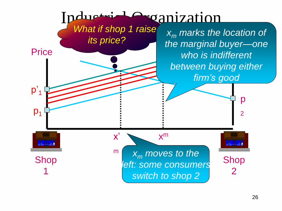
What if shop 1 raises
its price?
p’1
x’
m xm moves to the
left: some consumers
switch to shop 2
xm marks the location of
the marginal buyer—one
who is indifferent
between buying either
firm’s good

27
Industrial Organization
Shop
1
Shop
2
Price Price
p1
p2
xm
How is xm
determined?
p1 + txm = p2 + t(1 - xm) 2txm = p2 - p1 + t
xm(p1, p2) = (p2 - p1 + t)/2t This is the fraction
of consumers who
buy from firm 1So demand to firm 1 is D1 = N(p2 - p1 + t)/2t
There are N consumers in total

28
Industrial OrganizationProfit to firm 1 is p1 = (p1 - c)D1 = N(p1 - c)(p2 - p1 + t)/2t
p1 = N(p2p1 - p12 + tp1 + cp1 - cp2 -ct)/2t
Differentiate with respect to p1
p1/ p1 =N
2t(p2 - 2p1 + t + c) = 0
Solve this
for p1
p*1 = (p2 + t + c)/2
What about firm 2? By symmetry, it
has a similar best response function.
This is the best
response function
for firm 1
p*2 = (p1 + t + c)/2This is the best
response function
for firm 2

29
Industrial Organization
p*1 = (p2 + t + c)/2 p2
p1
R1
p*2 = (p1 + t + c)/2
R2
(c + t)/2
(c + t)/2
2p*2 = p1 + t + c
= p2/2 + 3(t + c)/2
p*2 = t + c
c + t
p*1 = t + c
c + t
Profit per unit to each firm is t
Aggregate profit to each firm is Nt/2

30
Industrial Organization
• Two final points on this analysis.
1. t measures transport costs. It is also a measure of the value
consumers place on getting their most preferred variety.
– when t is large competition is softened
• and profit is increased
– when t is small competition is tougher
• and profit is decreased
2. Locations have been taken as fixed.
– if product design can be set by the firms, firms must
balance temptation to be close (business stealing)
against desire to be separate (softer competition).
31
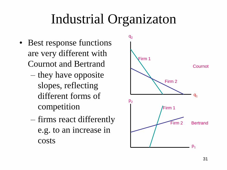
Industrial Organizaton
• Best response functions
are very different with
Cournot and Bertrand
q2
q1
p2
p1
Firm 1
Firm 1
Firm 2
Firm 2
Cournot
Bertrand
– they have opposite
slopes, reflecting
different forms of
competition
– firms react differently
e.g. to an increase in
costs

32
Industrial Organization
q2
q1
p2
p1
Firm 1
Firm 1
Firm 2
Firm 2
Cournot
Bertrand
– Suppose Firm 2’s costs increase.
– This causes Firm 2’s Cournot
best response function to fall.
• at any output for firm 1, firm
2 now wants to produce less
– Firm 1’s output increases and
Firm 2’s falls
aggressive
response by
firm 1
– Firm 2’s Bertrand best
response function rises.
• at any price for firm 1, firm 2 now
wants to raise its price
– Firm 1’s price increases as does
Firm 2’s.
passive
response
by firm 1
33
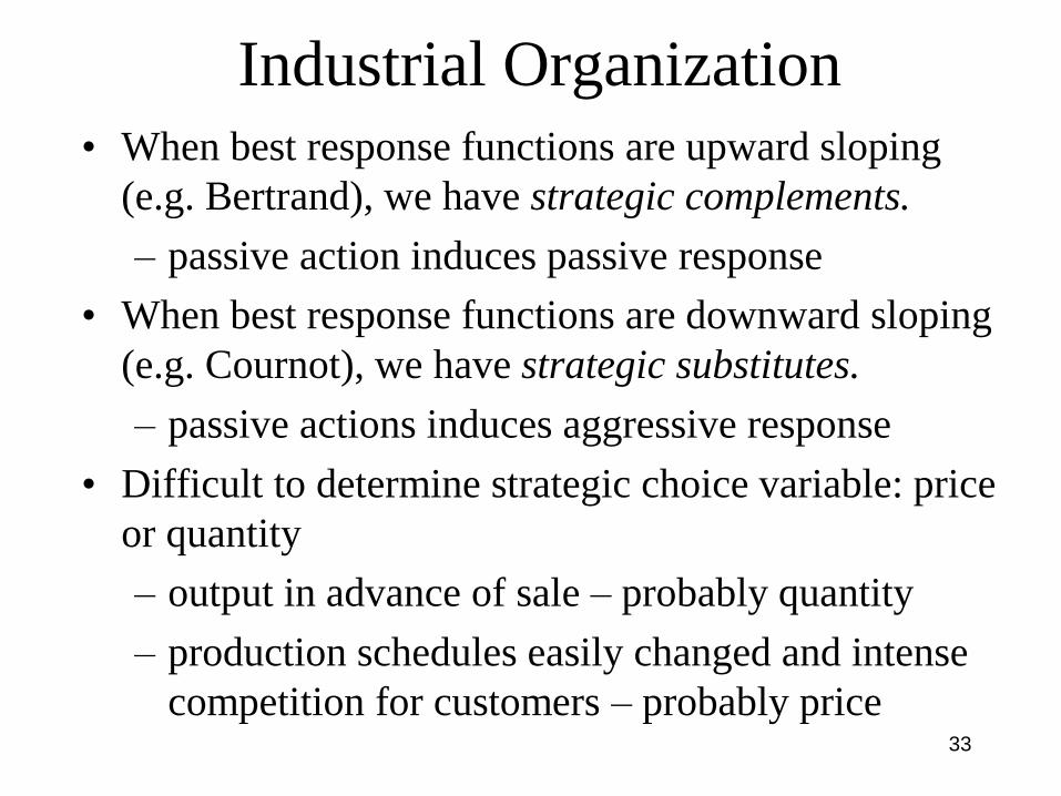
Industrial Organization
• When best response functions are upward sloping
(e.g. Bertrand), we have strategic complements.
– passive action induces passive response
• When best response functions are downward sloping
(e.g. Cournot), we have strategic substitutes.
– passive actions induces aggressive response
• Difficult to determine strategic choice variable: price
or quantity
– output in advance of sale – probably quantity
– production schedules easily changed and intense
competition for customers – probably price

34
Industrial Organization
• Read Chapter 11.