ecb a market-based approach to sector risk determinants and transmission in the euro area
DESCRIPTION
ECB working paper 2013TRANSCRIPT
Work ing PaPer Ser ieSno 1574 / auguSt 2013
a Market-baSed aPProach to Sector riSk deterMinantS
and tranSMiSSion in the euro area
Martín Saldías
In 2013 all ECB publications
feature a motif taken from
the €5 banknote.
note: This Working Paper should not be reported as representing the views of the European Central Bank (ECB). The views expressed are those of the authors and do not necessarily reflect those of the ECB.
MacroPrudential reSearch netWork

© European Central Bank, 2013
Address Kaiserstrasse 29, 60311 Frankfurt am Main, GermanyPostal address Postfach 16 03 19, 60066 Frankfurt am Main, GermanyTelephone +49 69 1344 0Internet http://www.ecb.europa.euFax +49 69 1344 6000
All rights reserved.
ISSN 1725-2806 (online)EU Catalogue No QB-AR-13-071-EN-N (online)
Any reproduction, publication and reprint in the form of a different publication, whether printed or produced electronically, in whole or in part, is permitted only with the explicit written authorisation of the ECB or the authors.This paper can be downloaded without charge from http://www.ecb.europa.eu or from the Social Science Research Network electronic library at http://ssrn.com/abstract_id=1913659.Information on all of the papers published in the ECB Working Paper Series can be found on the ECB’s website, http://www.ecb.europa.eu/pub/scientific/wps/date/html/index.en.html
Macroprudential Research NetworkThis paper presents research conducted within the Macroprudential Research Network (MaRs). The network is composed of economists from the European System of Central Banks (ESCB), i.e. the national central banks of the 27 European Union (EU) Member States and the European Central Bank. The objective of MaRs is to develop core conceptual frameworks, models and/or tools supporting macro-prudential supervision in the EU. The research is carried out in three work streams: 1) Macro-financial models linking financial stability and the performance of the economy; 2) Early warning systems and systemic risk indicators; 3) Assessing contagion risks.MaRs is chaired by Philipp Hartmann (ECB). Paolo Angelini (Banca d’Italia), Laurent Clerc (Banque de France), Carsten Detken (ECB), Simone Manganelli (ECB) and Katerina Šmídková (Czech National Bank) are workstream coordinators. Javier Suarez (Center for Monetary and Financial Studies) and Hans Degryse (Katholieke Universiteit Leuven and Tilburg University) act as external consultants. Fiorella De Fiore (ECB) and Kalin Nikolov (ECB) share responsibility for the MaRs Secretariat.The refereeing process of this paper has been coordinated by a team composed of Gerhard Rünstler, Kalin Nikolov and Bernd Schwaab (all ECB). The paper is released in order to make the research of MaRs generally available, in preliminary form, to encourage comments and suggestions prior to final publication. The views expressed in the paper are the ones of the author(s) and do not necessarily reflect those of the ECB or of the ESCB.
AcknowledgementsThe author is grateful to António Antunes, Diana Bonfim, Jörg Breitung, Ben Craig, Frank De Jonghe, Olivier De Jonghe, Jonas Dovern, Salvatore Dell’Erba, Dries Heyman, Peter Pedroni, Ivan Petrella, Andreas Pick, Nuno Ribeiro, Paulo Rodrigues, Elisa Tosetti, Rudi Vander Vennet and participants at the XX International Tor Vergata Conference on Money, Banking and Finance, the 24th Australasian Finance & Banking Conference and at seminars at Banco de Portugal, Bank of England and Banco Central de Chile for helpful comments and suggestions. The views expressed in this paper as those of the author and do not necessarily reflect those of Banco de Portugal or the Eurosystem. All remaining errors those of the author.
Martín SaldíasBanco de Portugal; e-mail: [email protected]

Abstract
In a panel data framework applied to Portfolio Distance-to-Default series of
corporate sectors in the euro area, this paper evaluates systemic and idiosyncratic
determinants of default risk and examines how distress is transferred in and between
the financial and corporate sectors since the early days of the euro. This approach
takes into account observed and unobserved common factors and the presence of
different degrees of cross-section dependence in the form of economic proximity.
This paper contributes to the financial stability literature with a contingent claims
approach to a sector-based analysis with a less dominant macro focus while being
compatible with existing stress-testing methodologies in the literature. A disag-
gregated analysis of the different corporate and financial sectors allows for a more
detailed assessment of specificities in terms of risk profile, i.e. heterogeneity of busi-
ness models, risk exposures and interaction with the rest of the macro environment.
JEL classification: G01, G13, C31, C33.
Keywords: Macro-prudential Analysis; Portfolio Credit Risk Measurement; Common
Correlated Effects; Contingent Claims Analysis.
1
Non-technical Summary
The study of interactions and feedback effects between the financial system and the real
economy is among the most challenging topics of research on financial stability. Along
these lines, this paper presents a framework to analyze distress risk in the financial sector
and the non-financial corporate sectors in the euro area. The analysis takes into account
their strong sectoral linkages and co-movement across sectors.
In the first part, the paper describes a methodology to compute forward-looking risk
indicators at sector-level based on Contingent Claims Analysis with information from
balance sheets and prices of stock indices and index options. A sector-wide analysis for
the euro area, as opposed to a country-based analysis, emphasizes the increasing degree
of integration in financial markets due to the introduction of the euro and also a greater
Europeanization of corporate and financial activities.
The second part of the paper analyzes the properties of the resulting Portfolio Distance-
to-Default series and sets up an econometric model that incorporates the cross-section
dependence of sectoral risk. Cross-section dependence features in the data as a result of
the effect of unobserved common factors at place, such as the macroeconomic and finan-
cial conditions or unobserved risk spillovers originated in the various forms of “economic
proximity”. The results show that distress risk in the corporate sector comprises a station-
ary idiosyncratic component and a non-stationary common factor, which flows around a
long-run equilibrium, with temporary deviations caused by shocks in the macro-financial
environment, at sector-specific level or as a result of the interplay between sectors.
The econometric results find evidence supporting a more relevant role of sector-specific
variables as sectoral risk determinants in the overall corporate sector at the expense of
the direct impact from macro-financial variables. The macroeconomic and financial com-
mon variables are captured as unobserved common effects, averaged out by heterogeneous
affects across sectors or smoothed out by construction of the Distance-to-Default series.
This empirical finding challenges much of the literature that focuses mainly on macroe-
conomic risk drivers and tends to ignore sector-specific characteristics and interactions.
The paper also shows that the effect and magnitude of risk drivers across sectors is highly
heterogeneous and that this feature should be taken into account for policy purposes, e.g.
the design of stress testing analytical tools.
2
1. Introduction
Due to the financial and economic crisis that started in Summer 2007, research on fi-
nancial stability is facing new challenges and embarked on a growing agenda. There is a
consensus to develop new and enhanced measures to understand global financial networks
and to provide policy making with improved analytic tools (Financial Stability Board,
2010). The growing literature on financial stability has been urged to expand the focus
and to incorporate the interaction between the financial system and the rest of the eco-
nomic agents and sectors.
This paper addresses the importance of heterogeneity in terms of risk determinants
and risk transmission across corporate sectors in the euro area. I propose a model where
risk in the corporate sector, comprising the financial sector (banks and insurance compa-
nies) and the non-financial corporate sector (10 supersectors), is determined by general
economic and financial markets conditions and by sector-specific risk drivers. The first
step in this paper consists in generating forward-looking sector-level risk indicators based
on Contingent Claims Analysis, a market-based indicator. Then, an analytic framework
using the Common Correlated Effects (CCE) estimator from Pesaran (2006) is provided,
allowing to study the determinants and diffusion of risk across sectors and over time,
in addition to those coming from other sector-specific determinants and also from the
macroeconomic environment and the financial markets.
The results show first that aggregate corporate default risk comprises a stationary
idiosyncratic factor and a non-stationary common element that drives the deviations of
the former from a long-term equilibrium. Results of the econometric model show that
shocks originated in the macroeconomic and financial environment have limited relevance
on idiosyncratic sectoral risk when cross-section dependence is accounted for and the
common element is filtered out. This result is partly driven by the market-base nature
of the risk indicator under analysis and more importantly because sectoral risk responds
more significantly to sector-specific shocks, including proximity-driven risk spill-overs.
Results also reveal a high degree of heterogeneity in terms of sensitivity and direction
of the effects both from macro-financial variables and from sector-specific risk-drivers.
These results show that a macro-only focus of the analysis of financial stability would be
misleading for policy if cross-section dependence and sectoral heterogeneity is ignored.
A large amount of the emerging literature has focused mainly on the effects of macroe-
conomic shocks on banking stability, while some work also addresses vulnerabilities in
3

the corporate sector at aggregate level. These studies vary significantly in terms of the
empirical methods applied, the sectors and macroeconomic variables of study, and the
assumptions about the direction of shocks, but they all show this strong macro analytic
focus. As an example, De Graeve et al. (2008) develop a model of shocks and feedback
effects between the real sector (through monetary policy shocks) and the financial system
with no prior assumptions about the direction of shocks. On the same topic, Castren
et al. (2009) propose a model to assess effects from macroeconomic variables, with no
feedback, on credit risk measures of Large and Complex Banking Groups (LCBG) in the
euro area.
Focusing on the interdependence between macro variables and the non-financial cor-
porate sector, Asberg and Shahnazarian (2009) use an error correction model to assess
sensitivity in the aggregate Swedish corporate sector to shocks in variables such as in-
dustrial production, interest rates and consumer prices. Carling et al. (2007) use a panel
data model to assess empirically the impact of macroeconomic and firm-specific shocks on
default probabilities also in the Swedish corporate sector. Bruneau et al. (2008) analyze
links in both directions between non-financial companies and macroeconomic variables,
including financial shocks, for the French economy. Castren et al. (2010) expand their
previous work and study global macro and financial shocks on the same credit risk mea-
sures of the euro area financial and corporate sectors separately, using satellite-GVAR
models. Castren and Kavonius (2009) propose a different approach and include in their
analysis the linkages among the rest of economic sectors, e.g. households, government
and rest of the world, using a network of balance sheet exposures and risk-based balance
sheets.
Even though the assessment of the effects of general economic conditions on overall
corporate risk is highly relevant for financial stability, understanding also the credit risk
relationships within the corporate sector with a less macro focus is certainly not negli-
gible, yet it has not been extensively studied. As credit risk events at individual firm
level are linked via sector-specific and general economic conditions (Zhou, 2001), so is
risk propagation across corporate sectors through a number of complex channels. In ad-
dition, sectoral risk features and responses to common shocks are heterogeneous, hence
neglecting this heterogeneity may be misleading in terms of overall credit risk manage-
ment (Hanson et al., 2008), financial stability analysis and policy decisions.
During the Asian crisis in 1997, an over-leveraged and poorly profitable corporate sec-
4
tor put the Asian financial system on the verge of collapse and triggered a deep economic
crisis (Pomerleano, 2007). The current crisis has highlighted the role of banks in hetero-
geneous risk transmission to the corporate sector in developed economies either directly
through credit constraints or indirectly through higher financing costs, less investment
counterparts or even second round effects on demand. Castren and Kavonius (2009) show
that the bilateral linkages between the financial system and the corporate sector in euro
area (measured by balance sheets gross exposures) are the most significative and take
place through both the credit channel and the securities markets. In addition, the degree
of correlation and default transmission between non-financial corporate sectors is high
due to complementary or similar business lines, e.g. Telecoms and Technology, Utilities
and Oil & Gas.
Sectoral risk relationships and their dynamics have previously been analyzed using
market-based indicators in Alves (2005) with a VAR approach and in Castren and Kavo-
nius (2009) using network analysis. Their results highlight important cross-dynamics
across sectors in addition to the impacts viewed as systemic and generated by macroeco-
nomic variables. However, the high degree of aggregation in these papers is likely to have
neglected important linkages within the corporate sector and with the financial system
(Castren and Kavonius, 2009) and may also have ignored sector-specific elements of de-
fault risk (Chava and Jarrow, 2004), which provide an additional motivation to this study.
Additionally, the dimension limitations of a traditional VAR model leaves some unob-
served effects unaccounted for (Alves, 2005). In a recent paper, Bernoth and Pick (2011)
model linkages between the insurance and banking sectors and forecast their default risk
in presence of unobserved linkages and other common shocks using the CCE estimator1.
The risk transmission between the components of the financial sector (banks and insur-
ance) and additional non-financial corporate sectors and within the non-financial sector
is not directly tackled, leaving an important source of risk to be further analyzed.
For these reasons, this paper exploits recent techniques to deal with panel data in
presence of cross-section dependence (CD) and unobserved factors using the Common
Correlated Effects (CCE) estimator introduced in Pesaran (2006). This study gener-
ates the following contributions to the literature. First, it proposes a methodology to
build sectoral risk indicators using balance sheet, market-based and, most notably, op-
1The authors use backward-looking Distance-to-Default series computed for a very large number ofindividual institutions and aggregate them into series of weighted averages and lower quantiles to computesystemic wide forecasts.
5
tion prices information. These series become forward-looking and allow for a wide range
of stress-testing exercises. Then, the paper provides an analytic framework to study risk
determinants and transmission at sector level in the euro area by taking into account
both the cross-section dimension as well as the time series dimension of risk, which has
been long neglected in the literature due to lack of a suitable multivariate methodology.
The rest of this paper is structured as follows. Section 2 introduces the sector-level risk
indicator and the methodology to compute it for aggregate sectors. Section 3 describes
the sample of sectors and companies included in the analysis and the properties of the
sectoral risk indicators. Section 4 describes the analytic framework of risk determinants
and diffusion using the CCE estimator and other panel data methods applied in the
empirical analysis. The results of the former are explained in Section 5 and Section 6
concludes.
2. Sectoral Risk Measure for the Euro Area’s Financial and Corporate Sec-
tors
The risk measures chosen in this paper to analyze sector-level stress in the euro area are
Portfolio Distance-to-Default (DD) series, namely forward-looking DD series built using
aggregated balance sheet information of individual companies by sector and market infor-
mation of their corresponding indices. DD series make part of the set of risk indicators
based on Contingent Claims Analysis (CCA)2. DD series were initially developed and
disseminated for commercial purposes by Moody’s KMV using market-based and balance
sheet information to assess credit risk in individual companies (Crosbie and Bohn, 2003).
They indicate the number of standard deviations at which the market value of assets
is away from a default barrier defined by a given liabilities structure. A decrease in DD
reflects a deteriorating risk profile, as a result of the combination of the following factors:
lower expected profitability, weakening capitalization and/or increasing asset volatility.
Variants of this indicator are increasingly used to analyze credit risk of aggregated cor-
porate and macro sectors. Gray and Malone (2008) provide a comprehensive overview of
techniques and applications.
2Contingent Claims Analysis (CCA) is an analytic framework whereby a comprehensive set of financialrisk indicators is obtained by combining balance sheet and market-based information including expectedloss, probability of distress, expected recovery rate and credit spread over the benchmark risk-free interestrate. It is based on the Black-Scholes-Merton model of option pricing and has three principles: 1) Theeconomic value of liabilities is derived and equals the economic value of assets, where liabilities equalsdebt plus equity; 2) Liabilities in the balance sheet have different priorities and risk; and 3) The assetsdistribution follows a stochastic process.
6
At aggregate corporate sector-level exclusively, DD signals the probability of gener-
alized distress or joint failure in a given sector or industry. Despite strong modelling
assumptions3, empirical research has shown that aggregate DD dynamics contains infor-
mational signals of market valuation of distress and therefore DD is a valuable monitoring
tool of the risk profile in the financial and non-financial corporate sectors (Gropp et al.,
2009; Vassalou and Xing, 2004).
Since the same principles of CCA can be applied to aggregation of firms, the analysis
of an entire corporate sector becomes the analysis of a portfolio of companies. In empiri-
cal terms, individual company information needs to be aggregated together into a single,
tractable and highly representative indicator by corporate sector, where its composition
must be clearly defined.
As for aggregation, most papers in the literature compute the median or either the
weighted or unweighed average of DD or EDF series4 for a large and changing sample
of companies. This methodology produces an indicator that highlights the intensity and
overall risk outlook in the sector but may overemphasize the large players or may par-
tially neglect interdependencies among portfolio constituents (Alves, 2005). Examples of
this approach are found in Alves (2005); Bernoth and Pick (2011); Carlson et al. (2008);
Castren and Kavonius (2009); Castren et al. (2009, 2010) and Asberg and Shahnazarian
(2009).
By contrast, this paper’s aggregation approach are Portfolio DD series, following
research on financial systemic risk in Cihak and Koeva Brooks (2009); De Nicolo and
Tieman (2007); Muhleisen et al. (2006); Echeverrıa et al. (2009); De Nicolo et al. (2005)
and Saldıas (2012). This methodology treats the set of companies by sector as a single en-
tity, it aggregates balance sheet and market data and incorporates the assumed portfolio
volatility before computing the DD series. Appendix A contains a complete explanation
of Portfolio DD’s derivation and data requirements.
The Portfolio DD series obtained using this methodology have several interesting fea-
tures. Portfolio DD enhances the informational properties of average DD series, since
3These assumptions are concerned mainly with those inherent in the Merton-based model (e.g. log-normal distribution of assets, constant asset volatility, etc.) and also the liability structure.
4Expected Default Frequency (EDF) is a credit measure based on CCA and adapted by Moody’sKMV to reflect actual default distributions.
7
it does not only capture company size but also interdependencies among the portfolio
constituents. It may be considered as the upper bound of joint distance to distress (the
lower bound in terms of joint probabilities of distress) in normal times (De Nicolo and
Tieman, 2007) but it tends to converge with the average DD in times of stress, when
equity market volatility and correlation are higher. This feature illustrates quick reaction
of the indicator to market events and shows the generalized increase in returns covariance
in a sector during distress times, even if fundamentals of portfolio constituents may be
solid. Aggregated company fundamentals embedded in the indicator are informative of
longer-term trends of sectoral risk (see Saldıas (2012) for an extensive discussion).
Finally, since aggregation of company information is conducted before computing the
risk indicator, calibration of Portfolio DD also allows to add more easily forward-looking
properties from option markets via option implied volatilities from EURO STOXX in-
dices, which also circumvent assumptions about constituents’ returns correlations. Port-
folio DD acquires more responsiveness to early signs of sector-level distress and hence
serves to stress scenarios5.
The second empirical issue deals with the sector classification and the selection of
constituent companies in the Portfolio DD. Research based on median and average DD
series tackles only the former issue6 and then picks the largest sample available with
breaks in sample composition. This approach is however likely to be affected by spurious
variation due to classification changes affecting large companies (Alves, 2005) or due to
relevant corporate events, including M&A, spin-offs or delistings.
This paper choice for sector classification is the Industry Classification Benchmark
(ICB) at Supersector level7. ICB is a widely used and comprehensive company classi-
fication system jointly developed by FTSE & Dow Jones Indexes to aggregate traded
companies according to their main sources of revenue, as reported in audited accounts
and directors’ reports. The grouping at Supersector level is wide enough to ensure a large
degree of homogeneity in business models and sectoral characteristics in each portfolio
vis-a-vis grouping at Industry level and it is narrow enough not to blur interactions among
them, as it is the case at Sector level. An additional and very important reason for this
5This paper does not include average DD series computed using option price information as describedin Saldıas (2012) since there are not enough single equity options traded for all companies in this largesample.
6In general, they adopt systems linked to those used for National Accounting.7Even though Industries, Supersectors and Sectors are clearly differentiated as ICB Categories, the
use of these terms in this paper will uniquely refer to Supersectors.
8

grouping criterion is the fact that Portfolio DD are built so they include option-based
information and the most liquid option market for sector indices are the EURO STOXX
options on ICB-based Supersectors traded at Eurex.
Constituent lists in each Supersector Index are revised every quarter and reclassifica-
tions take place whenever relevant corporate events occur. In order to minimize possible
spurious variation in the risk indicator, the portfolio constituents take into account these
changes and make some assumptions when required. Appendices C and E describe in
detail the company sample by portfolio and all additional assumptions made to ensure
the portfolios’ accuracy, including exclusions and ad-hoc reclassifications.
3. Sample and Preliminary Analysis
The sample consists of 12 out of the 19 EURO STOXX Supersectors8. These sectors are
the most relevant by different measures of size, e.g. assets, market value, employment.
They have been included in the sample according to two main criteria in order to ensure
the best informative quality of their market-based indicators, namely: 1) availability
and liquid trading volume of their associated Eurex Index options quotes9; and 2) stock
market capitalization of the their corresponding Supersector STOXX Indices at Deutsche
Boerse. Table 1 briefly lists them and provides relevant market information.
[Insert Table 1 here]
The dataset comprises monthly observations between December 2001 and October
2009 (95 observations per Supersector). This period is characterized by an increasing
degree of integration in European financial markets due to the introduction of the euro
and a greater europeanization of corporate activities (Veron, 2006). Recent trends and
findings suggest that equity markets integration has lead to a reduction of home bias and
to an increase of sector-based equity allocation strategies at the expense of country-based
8The remaining seven sectors are Construction & Materials, Travel & Leisure, Personal & HouseholdGoods, Financial Services, Retail, Basic Resources and Real Estate. They were left out of the samplebecause of two reasons. First, their options series start late in the sample and are comparatively lessliquid, with several months without reported trading. In addition, there are breaks in the data. Forinstance, the STOXX indices shifted methodology from Dow Jones Global Classification Standard toIndustry Classification Benchmark (ICB)in September 2004, affecting the composition of the Personal& Household Goods and Travel & Leisure Supersectors and making their corresponding DD series notcomparable. In addition, the Real Estate Supersector was elevated to Supersector in 2008, after havingbeen part of the Financial Services Supersector, which constitutes another break in the data.
9The DD series were initially computed on a daily basis and then averaged to obtain monthly data.Volatilities from a GARCH(1,1) model applied to the respective Supersector index were used to completethe volatilities series when unavailable.
9

strategies (European Central Bank, 2010; Cappiello et al., 2010). These developments
give support to the aggregation of company risk indicators into portfolios for the euro
area as a whole and they provide a first tentative and equity-driven explanation to strong
comovement of the series over time, as can be seen in Figure 1.
[Insert Figure 1 here]
Figure 1 displays together the 12 sectoral DD series and the EURO STOXX 50, the
benchmark stock index in the euro area. Being a market-based indicator, DD series
move along together with the stock market benchmark. In fact, they visibly lead it. This
feature serves to illustrate the forward-looking properties of the DD series from option
prices as inputs (Saldıas, 2012). The DD series anticipate turning points along the entire
period of analysis. During the recent crisis, they reach their bottom at the end of 2008
while the EURO STOXX 50 only picks up after the end of the first quarter of 2009.
[Insert Figures 2 and 3 here]
The DD series do not show a clear linear trend but they suggest a high degree of co-
movement along the whole time span and correlation among them is very high on average
and statistically significant both in levels and in first differences. Figures 2 and 3 show
the median and quartile regions of bilateral correlation coefficients across sectors using
24-month moving windows of DD series levels and first differences in order to illustrate
the changing pattern of cross-section sectoral risk correlation over time. Median correla-
tion is high in the entire sample but it shows greater dispersion in tranquil times where
idiosyncratic drivers of sector risk dominate. However, median correlation increases and
its dispersion across sectors narrows significantly in episodes of higher stress in financial
markets, e.g. in the aftermath of the dot-com bubble burst in 2002; after the subprime
crisis start in August 2007; and especially in the third quarter of 2008, after Lehman
Brothers’ collapse. At the end of the sample, median risk correlation across sectors re-
mains high, but there is greater dispersion suggesting somehow a moderation in the role
of sector-wide risk drivers.
Table 2 reports preliminary cross-section dependence tests applied to levels and first
differences of DD series regressed on sector intercepts. High values of all these statis-
tics reject the null hypothesis of cross-section independence and confirm the results of
graphical inspection: DD series show a high degree of cross-section dependence even if
the series are differentiated.
[Insert Table 2 here]
10

In addition to strong comovement and high correlation among the series, the results in
Table 2 suggests that it is very likely to have both observable and unobservable common
factors at place. Variables from the macroeconomic environment and from financial mar-
kets are strong candidates as common factors and induce strong cross-section dependence
across sectors (Alves, 2005; Holly et al., 2010).
Additionally, this particular dynamics in DD series may also be caused by risk dif-
fusion across sectors, which in turn may come in form of “economic proximity” and
additional unobserved factors. Risk transmission is likely to be variant across sectors and
change in time and the nature of sectoral economic proximity comes from many sources.
Similarity of business lines is a first source of this type of relationship and it includes
common customer base and competition relationships. Financial linkages are another
source of shock spillovers and take place not only between the financial sector and the
non-financial corporates, but also between non-financial companies through credit chains
and counterparty risk relationships. See results in Couderc et al. (2008); Das et al. (2007);
Jarrow and Yu (2001) and Veldkamp and Wolfers (2007) for in depth discussions of these
relationships10. Finally, other complementarity relationships are also relevant. They can
take place through technological linkages (Raddatz, 2010) or collateral channels of risk
through the securities channel (Benmelech and Bergman, 2011).
4. The Econometric Model
This section describes in detail the econometric model to analyze the risk determinants
and transmission across the euro area’s financial and corporate sectors using the Portfolio
Distance-to-Default series constructed following the methodology presented in Section 2
and Appendix A.
Under the potential presence of cross-section dependence in the DD series, a suitable
econometric method is the Common Correlated Effects (CCE) estimator introduced in
Pesaran (2006) and further extended in Pesaran and Tosetti (2011) and Chudik et al.
(2011). CCE is a consistent econometric panel data method in presence of different de-
grees of cross-section dependence coming from common observed and single or multiple
unobserved factors and from proximity-driven spillover effects (Pesaran and Tosetti, 2011;
Chudik et al., 2011). The CCE method also tackles methodological limitations of other
10Bernoth and Pick (2011) also explore spatial effects in risk diffusion between banking and insurancesectors using DD series of individual institutions from Asia, North America and Europe. In this paper,the spatial component is not relevant since portfolios are constructed bundling together only euro areacompanies.
11
econometric models when modelling interrelationships across sectors due to large N di-
mension, e.g. VAR (Pesaran et al., 2004).
This method is computationally simple and has satisfactory small sample proper-
ties even under a substantial degree of heterogeneity and dynamics, and for relatively
small time-series and cross-section dimensions (N = 12 and T = 95 in this case). It is
also consistent in presence of stationary and non-stationary unobserved common factors
(Kapetanios et al., 2011) and more suitable for this dataset than a SURE model due to
the possible presence of time-variant correlation patterns, as suggested for this case in
Figures 2 and 3.
The general model specification is a dynamic panel and takes the following form:
DDi,t = αidt + βiXi,t + ui,t, i = 1, . . . , N ; t = 1, . . . , T (1)
where DDi,t is the Distance-to-Default of sector i at time t. The vector dt includes the
intercepts and a set of observed common factors that capture common macroeconomic
and financial systemic market shocks. Xi,t is the vector of sector-specific regressors, in-
cluding lags of i’s own Distance-to-Default, the direct risk spill-overs from “neighboring
sectors” and other sector-specific variables. All coefficients are allowed to be heteroge-
neous across sectors11 and all remaining factors omitted in the specification and other
idiosyncratic risk drivers are captured in the error term ui,t.
The CCE estimator can be computed by OLS applied to sector-individual regressions
where the observed regressors are augmented with cross-sectional averages of the depen-
dent variable and the individual-specific regressors. The CCE estimator provides two
versions, namely the CCE Pooled estimator (CCEP) and the CCE Mean Group estima-
tor, of which only the latter will be reported because of slope heterogeneity and no need
for CCEP efficiency gains in this case.
4.1. Macroeconomic and Financial Risk Determinants
A set of five exogenous variables is included in the model in order to control for deter-
minants originated in the macroeconomic environment and to capture risk sensitivity to
common shocks in financial markets. A number of papers quoted in Section 1 have doc-
11See for instance results in Castren et al. (2010) for a more detailed, yet not strictly comparable,discussion of heterogeneous impact of macro variables on distress of corporate sectors, which are definedusing the European classification of economic activities (NACE).
12
umented the explanatory power of macroeconomic and financial variables in corporate
default risk, thus their omission could bias the results of the parameter estimation in the
model.
The model takes macrofinancial determinants as exogenous and chooses to ignore pos-
sible feedback effects to the macrofinancial environment. Examples of this approach and
additional explanation for this modelling decision can be found in Castren et al. (2010)
and Castren et al. (2009). Accordingly, the econometric specification first includes the
annual rate of change of the Industrial Production Index (∆PIt) and the Harmonised
Index of Consumer Prices (∆CPt) in the euro area, in order to capture the effect of
demand shocks. Brent Oil (1-Month Forward Contract) prices changes denominated in
euro (OILt) detect supply shocks. The short-term benchmark interest rate is also in-
cluded using the 3-Month Euribor Rate (R3Mt), which also reflects developments in the
money market affecting the financial sector and serves as a reference for corporate debt
yields and borrowing. They also are linked to corporate asset return growth. Finally,
the Chicago Board Options Exchange Volatility Index (V IXt) is included to gauge global
equity market sentiment. The VIX index tends to be low when markets are on an upward
trend and tends to increase with market pessimism, therefore its relationship with DD
series is expected to be negative.
4.2. Sector-specific Risk Determinants
4.2.1. Sector-specific Risk Determinants
The model includes four other sector-specific regressors computed for each ICB Supersec-
tor Index12, namely: 1) the annual rate of change of the Price-Earnings Ratio, ∆PEt; 2)
the annual rate of change in Dividend Yields, ∆DYt, 3) the Return On Assets, ROAi,t;
and 4) the monthly log excess return on each index’s daily price return relative to the
EURO STOXX 50 Index, EXRETi,t.
Earnings, as measured by Price-Earnings Ratio, and profitability, as measured by
ROA, are studied extensively in the corporate bankruptcy literature. Indeed, results in
Shumway (2001); Beaver et al. (2005) and Chava and Jarrow (2004) show that higher
earnings are traditionally associated with lower distress probabilities, in spite of a weaker
informational ability detected in recent years due to higher frequency in earnings restate-
ments and the possibility of data manipulation (Dechow and Schrand, 2004). Return
12See Appendix D for details of these determinants and the rest of macro-financial variables.
13
On Assets (ROA) incorporates further information about profitability and the ability of
the companies in a given sector to generate returns. Dividends traditionally serve to as-
sess and infer corporate performance. Recent work by Charitou et al. (2011) shows that
dividend payment initiations or increases tend to reduce corporate default and tend to
raise the assets returns for several subsequent periods. However, specially in the financial
sector, aggressive dividend policies may also encourage risk-taking and erode the capital
base of a company or sector (Acharya et al., 2011). Excess returns are a purely market-
based measure of relative performance at aggregate level and is motivated by results in
Campbell et al. (2008).
No additional firm-level information or sector specific indicator are included in the
model since the DD construction already includes either directly or indirectly the most
relevant variables of sector risk, i.e. market-implied assets’ returns and volatility and
aggregated leverage (Bernoth and Pick, 2011; Gropp et al., 2004).
4.2.2. Neighboring Sectors’ Risk Spillovers
The risk spill-over across sectors is studied using DD series from neighboring sectors. For
a given sector i, the neighboring effect is defined by:
DDni
i,t =1
ni
n∑j=1
DDj,t (2)
DDn
i,t is a simple average of the DD series of the n “neighbours” (DDj,t) of sector i.
For each sector i, the number of neighbors and weighting of their corresponding DD
series are determined by a contiguity matrix (see Table 3) derived from ad-hoc and prede-
fined neighborhood linkages among sectors13. Even though the definition of neighboring
sectors and cross-sectional dependence in the literature comes largely from spatial prox-
imity (Holly et al., 2011, 2010; Pesaran and Tosetti, 2011; Chudik et al., 2011), other
measures of proximity, from economic or social networks, are also used in recent research
(Conley and Topa, 2002; Conley and Dupor, 2003; Holly and Petrella, 2012).
13The contiguity matrix W is an N ×N nonnegative matrix, whose wi,j element is 1 if sectors i andj are considered neighbors and 0 otherwise. The number of neighbors for sector i is the sum of elementsalong row i. Although weighting criteria is not likely to affect the properties of the econometric approach(Chudik et al., 2011) and a valid alternative in this case could weigh DD series by implied assets from thecalibration, this paper assumes equal weights in the neighborhood average (1/n) because the nature ofthe business in each sector affects considerably the asset sizes, hence, asset-based weights could introducedistortion. In addition, there is no only and unambiguous way to determine relative importance of sectorsamong each other.
14

In the case of corporate sectors, the literature does not provide a definite metric to de-
termine neighborhood linkages, because sectoral relationships depend both on the choice
of sector classification and on the sectoral characteristics to be linked14. Pesaran et al.
(2004) argue that the aggregation error in this type of exercises can be minimized if the
cross-section units, i.e. sectors in this case, are similar and the weights are chosen care-
fully.
As a result, the approach in this model is ad-hoc and market-based. It relies on
similarity of business lines embedded in the ICB methodology and covers important and
overlapping dimensions of sectoral interdependencies, namely: balance-sheet exposures,
financial linkages, common accounting practices, technological linkages, etc.
Supersectors are first assumed to be neighbours if they belong to the same Industry,
an upper level of aggregation to Supersectors in the ICB methodology structure. For
instance, the Industry of Consumer Goods links the Supersectors of Automobiles & Parts
and Foods & Beverages while Banks and Insurance Supesectors are bundled together as
Financials.
The second proximity criterion used to aggregate series into neighbours is also based
on the ICB methodology but it relies on the most frequent company reclassifications
across Supersectors within or outside a given Industry during the time span used in the
paper. Under multiple business lines, company reclassifications take place mainly due
to changes in the main business line and also due to corporate actions such as spin-offs
or M&A. Examples of this were frequent in supersectors such as Industrial Goods &
Services, Oil & Gas and Utilities, which do not belong to the same ICB Industries.
[Insert Table 3 here]
5. Empirical Results
5.1. Cross-section Dependence and Non-stationarity Analysis
Preliminary analysis in Section 3 detected a high degree of comovement in DD series in
levels and first differences. This section takes a step further and extends the CD tests
14Most studies deal with manufacturing sectors data, excluding financials. For example, Conley andDupor (2003) study sectoral synchronization of output and productivity growth using factor demandlinkages as a metric for economic distance for US corporates and define the sectors of study using theSIC system. Holly and Petrella (2012) use input-output linkages and analyze the shock propagationacross manufacturing sectors.
15

to the rest of sector-specific variables in the panel allowing for different degrees of serial
correlation in the data. It also conducts stationarity analysis of the data for correct model
specification, taking into account the potential presence of CD15.
Table 4 reports CD statistics of residuals from ADF(p) regressions of theDD series and
the sector-specific variables, including the neighboring sectors’ DD series (DDn
i,t). Results
detect that DD series and the DDn
i,t present very high and positive average correlation
coefficients, above 60%, whereas correlation for dividend yields’ growth and Returns On
Assets are also large but in the range of 25% - 40%. Price-Earnings ratio growth show very
low correlation across sectors, with a coefficient of around 3%. Excess returns relative to
the benchmark index also shows a low, though negative average correlation coefficient of
-4% on average. CD test statistics, reported below, are in line with these results and are
highest for DD series and neighboring effects, and smaller yet significant for the rest of
the variables. These tests confirm the strong cross-section dependence in the data, with
arguably the exception of Price-Earnings ratio growth and the relative indexes’ excess
return.
[Insert Table 4 here]
In line of the results of CD tests, panel unit root tests for the DD series and the
sector-specific regressors need to take into account cross-dependence. Accordingly, Table
5 summarizes the CIPS panel unit root tests described in Appendix B.2. IPS test statis-
tics are also reported for robustness check and comparison. Both CIPS and IPS tests
reject unit roots in dividend yields’ growth, Price-Earnings ratio growth and excess re-
turns and do not reject the null in the case of ROA. Interestingly, the CIPS strongly reject
unit roots in the case of DD series and neighboring effects for all lag orders p, whereas
IPS tests seem to suggest non-stationarity in most cases tested. Given the substantial
degree of cross-section dependence detected in these series, the CIPS tests provide a more
reliable inference and these variables are also taken as I(0). These tests also point out to
the combination of non-stationary common factors and stationary idiosyncratic compo-
nents in the sectoral risk16. ROA is taken as I(1) and enters the model in first differences.
15See Appendix B for technical details of the tests described in this subsection.16The non-stationarity detected in DD series and DD-neighbors using IPS tests comes from the com-
bination of non-stationary common factors and stationary idiosyncratic components. This possibilityhas been verified by adopting the Panel Analysis of Nonstationarity in the Idiosyncratic and Commoncomponents or PANIC approach advanced by Bai and Ng (2004). This result is consistent with findingsin Alves (2005), and provides empirical support to the notion that aggregate sectoral risk evolves to along-run equilibrium, which is in turn affected temporarily by the macro-financial environment and thecross-sectoral dynamics captured by the CCE method.
16
Finally, individual ADF(p) unit root tests were run for the macro-financial variables
described in Section 4.1 which enter the model as exogenous regressors. Based on the
results of these tests reported in Table 6, the annual rates of change of the Industrial
Production Index (∆PIt) and the Harmonised Index of Consumer Prices (∆CPt) enter
the model as I(0) variables, while Brent Oil prices (OILt), the 3-Month Euribor Rate
(R3Mt) and the VIX Volatility Index (V IXt) are previously differentiated to enter the
model.
[Insert Tables 5 and 6 here]
5.2. Model Estimation
The results from estimation of Equation (1) are reported in Table 7. Columns [1] to
[3] are estimates of naıve OLS Mean Group (MG) models (Pesaran and Smith, 1995)
that neglect cross-section dependence (CD). Columns [4] to [6] are Common Correlated
Effects (CCE) estimates of these same model specifications, hence more suitable to the
CD properties analyzed in the previous section. Although MG estimates are likely to be
biased, they serve as a benchmark for the CCE estimates and also put into context the
relevance of CD in the model specification. They also serve to compare these results with
previous studies on determinants of aggregate sectoral risk. .
[Insert Table 7 here]
The most relevant finding from the estimation results is the limited relevance of shocks
originated in the macroeconomic and financial environment on DD, especially when CD
is accounted for. This result has several interpretations and does not necessarily mean
that sectoral risk is not affected by the macro-financial environment. First, business
cycle volatility is likely to be smoothed out in the construction of DD series or other
CCA risk measures (especially EDF). Indeed, as suggested in International Monetary
Fund (2011), some high-frequency indicators of distress have the ability to anticipate
the cycle, which is very likely in the case of instruments derived from equity and option
markets17. Marked-based indicators, such as DD, may also be less directly responsive
due to non-linearities in their interactions with macroeconomic and financial variables
(Sorge and Virolainen, 2006). In addition, macro-financial effects may impact sectoral
DD in a more indirect way, via market news already embedded in the DD inputs and/or
through cross-dynamics transmitting risk across industries (Alves, 2005). Lastly, even
17To test this hypothesis, I conducted a simple Granger-causality test using the industrial productiongrowth (PIt) and the average of DD series and found that indeed the DD series Granger-causes changesin activity up to one trimester.
17
though sector-specific coefficients may have individual statistically significant signs, they
are allowed to be heterogeneous across sectors and the effect across the panel members
may be averaged out (Eberhardt and Teal, 2010).
In particular, the VIX Volatility Index (V IXt), a measure of investors’ risk sentiment,
is statistically significant at five percent across all the MG estimates and shows a stable
and expected negative sign, indicating an increase in sector-wide risk, i.e. a drop in DD,
when equity markets become more volatile. However, in all models estimated using the
CCE method its effect on overall sectoral risk vanishes. This is not a surprising result,
as Bernoth and Pick (2011) report that the VIX Index is absent in their CCE-based
models when forecasting DD at firm-level for banks and insurance companies. A very
plausible explanation in this case is that option implied volatilities from index options
endow the sectoral DD with the forward-looking information embedded in the VIX Index.
The same holds true for the 3-month Money Market (Euribor) Rate, R3Mt, which
shows statistical significance at five percent level and a positive and stable coefficient only
if CD is ignored. The effect of short-term interest rates on sectoral risk was expected to
be negative if we consider them as a proxy of borrowing costs and risk premia. However,
since short-term interest rates are closely linked to the risk-free rate used to capture sec-
toral assets return growth in the DD computation via the yield curve, this feature is likely
to be dominant in the estimates in this case. In addition, several empirical studies link
the short-term interest rates to higher performance and make an empirical case for the
positive sign. This positive effect becomes nil when CD is considered, probably because
the unobserved common factors capture it. This result is at odds with findings in Asberg
and Shahnazarian (2009)18, where the authors use a single risk indicator for the whole
corporate sector, but consistent with those from Castren et al. (2010), where short-term
interest rates are in general insignificant across several corporate sectors studied individ-
ually.
Shocks from oil prices (OILt) do not exert any statistically significant effect but in
equation [3], when CD is omitted, and none when CD is taken into account. The first
result is not entirely at odds with the literature, as Alves (2005) finds that oil prices do
not affect but one of the seven sectors he includes in his study. Shocks from industrial
18In this paper, the authors analyze effects of macroeconomic shocks on the the median EDF of thewhole corporate sector in Sweden in a VEC model. This series is a I(1) variable, in line with the findingsdescribed in the stationarity analysis of this paper, but this analysis does not take into account theheterogeneity across sectors and the cross-section dependence is ignored.
18

production growth (PIt) are insignificant on DD even when CD is neglected, whereas
growth in consumer prices (CPt) affects negatively, as expected, on overall sectoral risk in
only one of the MG specifications, equation [1]. This impact becomes insignificant when
sector-specific regressors are included in the MG model in two of three cases when CD
is controlled for. Its corresponding coefficient equation [6] exerts a positive coefficient.
Again, the changing statistical significance in the MG models is a sign of specification
failure to account for unobserved common factors appropriately. In turn, lack of statis-
tical significance of these variables with CCE estimates show that the macro-financial
effects are very likely to be captured either by the unobserved common effects and/or the
set of sector-specific variables more accurately.
Sector-specific regressors on DD display better results in terms of stable and strong
statistical significance under CD, which challenges the macro dominant focus in the ex-
isting literature of financial stability and highlights the importance of market-based and
sector-level information and interactions for policy analysis of systemic risk. Among the
set of six sector-specific covariates, the market-based indicators show stronger relevance
as distress drivers than those computed using balance-sheet information under alternative
econometric methods. In particular, dividend yields’ growth (∆DYi,t) does poorly and
shows no statistical significance in all models. The Return On Assets (∆ROAi,t) and
Price-Earnings Ratio, ∆PEt, show expected positive signs in MG models, equations [2]
and [3], but become insignificant when the CCE method is applied, in line with findings
in Bernoth and Pick (2011).
Two sector-specific and market-based variables show strong and significant effects
regardless the econometric method used, which can be interpreted as evidence of the rel-
evance of market-based information about distress beyond common observed risk drivers.
The distress risk persistence, as proxied by the lag of the dependent variable DDi,t−1,
shows a large and significant positive sign across all models. The CCE estimates show
however smaller coefficients as additional regressors are included in the specifications.
These MG coefficients are larger, close to one, probably because MG estimates capture
also the non-stationary common components. The strong significance of this regressor
confirms results in the literature (Alves, 2005; Bernoth and Pick, 2011) and illustrates
the persistence in idiosyncratic sectoral risk even after controlling for CD. With more
economic relevance, the sectoral indices’ excess return relative to the EURO STOXX 50
Index, EXRETi,t, exerts strong effects on sector-wide distress. This variable shows a
positive and significant coefficient sign across all model specifications, illustrating that
19
outperforming sectors relative to the corporate sector as a whole results in higher re-
silience and thus lower distress risk.
Finally, the neighboring sectors’ risk lagged effect on DD19, DDn
i,t−1, is statistically
insignificant in the CCE-estimated model, while MG estimates in Model [3] do exhibit
a positive coefficient. This result implies that the risk impact in sectors with strong
linkages on other sectors does not work directly but is mainly captured as unobserved
common factor. It is also possible that the ad-hoc definition of neighboring sectors is
not sufficiently accurate and other sectoral dimensions than those described in Section
4.2.2 need to be explored to obtain a more reliable contiguity matrix in terms of direct
spillovers20.
Some of the overall results described so far are expected to vary across sectors due to
heterogeneous effects of the regressors and also possibly because unobserved cross-sectoral
and complex shocks alter the relationships with them. As the CCE modelling approach
allows to shed some light on this, Table 8 reports the results of model [6] at individual
sector-level. To recap, this model is the most comprehensive and includes all variables
described in Section 4.
[Insert Table 8 here]
At individual Supersector level, some macro-financial variables do affect DD series
but not necessarily with the same sign. As in the aggregate results, oil (OILt) and
consumer prices (CPt) are the only macroeconomic variables that fail to show also at in-
dividual level any effect on sectoral risk. Interest rates (R3Mt) do play a significant role as
proxy of borrowing costs and risk premia for the Media (MDI) supersector (-0.502), while
shocks from industrial production growth (PIt) exert a surprisingly negative effect on the
idiosyncratic component of risk in the Telecommunications (TLS) supersector (-0.027).
The significance of the VIX Index (V IXt) on distress in the Automobiles & Parts and
Industrial Goods & Services sectors with alternating signs, -0.133 and 0.029, respectively,
illustrate the possibility of heterogeneous responses at individual level and nil effect on
the average.
19Contemporary effects were not gauged do the risk of dealing with potentially strong endogeneity andlimited possibilities to find valid instruments for this regressor.
20Robustness checks have been conducted using matrices of return and volatility spillovers accordingto the methodology described in Diebold and Yilmaz (2012) to construct the contiguity matrices. Theresults did not change for all models’ specifications.
20

As for the sector-specific variables, dividend yields growth, ∆DYt, and Price-Earnings
Ratio growth, ∆PEt, and Return On Assets (∆ROAi,t) affect also heterogeneously across
Supersectors. For instance, the coefficients associated to dividend yields are significant
and surprisingly positive in the Telecommunications and Media sector. Price-Earnings
Ratio and Return On Assets growth affects only the Food & Beverages sector with ex-
pected positive signs while being irrelevant for the rest of Supersectors.
Mirroring aggregated results, the lag of the dependent variable, DDi,t−1, is highly
significant also at individual level, for all supersectors with the no exceptions, while the
sectoral indices’ excess returns, EXRETi,t, are significant for half of the sectors in the
sample, with a positive sign in all cases. Finally, the lagged neighboring risk effect, non-
significant overall, is a risk driver in two Supersectors, Telecommunications and Media,
with positive signs in both cases.
Finally, the econometric estimates worth mentioning is the higher goodness-of-fit of
CCE estimates, as measured by the lower Root Mean Squared Errors across all model
specifications. As it might be expected, the cross-section dependence test statistics re-
ported below display a remarkable decline when the CCE estimator is applied and there
is no significant evidence of remaining CD in the estimation residuals21. It is however
noticeable the negative sign in all ρ and CDP statistics for CCE estimates. Since these
indicators are based on the sum of pairwise correlation coefficients, the sign indicates
that negative correlation coefficients are more frequent and sizable after controlling for
CD22. Finally, the serial correlation tests show that residuals from all estimated models
are stationary both individually and jointly.
5.3. Robustness check
Column [7] in Table 7 reports results of a robustness check of model [6] using the Aug-
mented Mean Group (AMG) estimator, which shows very similar properties to CCE and
account for cross-section dependence by inclusion of a preassumed single “common dy-
namic process” in the sector regressions imposed with unit coefficient. AMG estimates
provide an alternative estimator under CD and obtain an explicit estimate for the un-
observed factors. This estimator has been developed in Eberhardt and Bond (2009) and
Eberhardt and Teal (2010) to deal with macro panels and been applied to estimate Total
21The CDP remains high enough not to reject the null of CD at 5%. This is due to the large timeseries dimension compared to the number of cross-section units.
22Although not reported, a closer look at bilateral residual correlations confirms this feature and that
this sum drives the value of the statistic, given that√
2TN(N−1) ≈ 1.
21
Factor Productivity (TFP) in cross-country production functions (Eberhardt and Teal,
2010) where TFP is the single common dynamic factor.
In our case, there are no priors to assume there is only one common factor driving the
idiosyncratic sectoral risk but this exercise serves to stress the robustness of the results
in the previous section. The estimates provide support to the previous results in terms of
the statistical significance of the lag of the dependent variable DDi,t−1, and the sectoral
indices’ excess return, EXRETi,t. In contrast to CCE estimates, the neighboring sectors’
risk lagged effect also appears relevant, with a negative coefficient, pointing out to a com-
peting nature of the relationships between sectors. Interestingly, three macroeconomic
variable also show statistical significance, namely the shocks from oil prices, industrial
production and consumer prices. Overall, these estimates confirm the CCE results, al-
though their goodness-of-fit is relatively lower and the residuals present some degree of
serial correlation.
6. Concluding Remarks
This paper presents a framework to analyze risk in the corporate sector that takes into
account their strong sectoral linkages and comovement. In a first part, the paper describes
a methodology to compute comprehensive forward-looking risk indicators at sector-level
based on Contingent Claims Analysis with information from balance sheets, equity mar-
kets and, more importantly, index option prices. The second part of the paper analyzes
the properties of the resulting Distance-to-Default series and sets up an econometric
model that incorporates the cross-section dependence of sectoral risk. This model allows
to study the determinants and diffusion of risk across sectors, including sector-specific
drivers, the macroeconomic and financial markets environment and proximity-driven risk
spill-overs.
In particular, the paper computes forward-looking Distance-to-Default DD series, a
market-based indicator, for 12 of the 19 financial and corporate sectors in the euro area as
defined by the EURO STOXX indices between December 2001 and October 2009. These
series show very good properties in terms of capturing cycles and episodes of distress.
The econometric analysis relies on the Common Correlated Effects estimator of Pesaran
(2006) in order to stress the importance of cross-section dependence (CD) in the risk
series over time, which is driven by common observed and unobserved factors.
Controlling for cross-section dependence among the Distance-to-Default series, the
22
first result of this analysis shows that sectoral risk comprises a stationary idiosyncratic
component and a non-stationary common factor. This result provides empirical support
to the notion that aggregate sectoral risk evolves to a long-run equilibrium, with tem-
porary deviations caused by the macro-financial environment, sector-specific shocks and
the cross-sectoral dynamics.
Results of the econometric model estimation using the Common Correlated Effects
(CCE) method find evidence supporting a more relevant role of sector-specific variables
as sectoral risk determinants in the corporate sector overall at the expense of the im-
pact from macro-financial variables. The sector-specific drivers include risk persistence,
measures of overall sectoral performance and also direct risk spill-overs from risk in re-
lated sectors. The macroeconomic and financial common variables are either captured
as unobserved common effects, averaged out by heterogeneous affects across sectors or
smoothed out by construction of the Distance-to-Default series. This empirical finding
challenges much of the literature that focuses mainly on macroeconomic risk drivers and
tends to ignore sector-specific characteristics and specially interactions either explicitly
or implicitly through an aggregate analysis of the whole corporate sector.
This study also provides empirical evidence of the high degree of heterogeneity as
concerns the relevance and responsiveness to the risk drivers used in the model, both in
macro-terms as in sector-specific terms. These results show that a macro-only focus of the
analysis of financial stability would be misleading for policy if cross-section dependence
and sectoral heterogeneity is ignored. These results make a case for a more disaggregated
analysis of risk across sectors without neglecting the inherent interactions that take place
among them. Subjects for further research include the inclusion of non-linearities in the
interaction of risk across sectors and exploring more accurate metrics to assess the direct
risk intersectoral linkages in order to extend the model to conduct stress tests.
23
References
Acharya, V. V., Gujral, I., Kulkarni, N. and Shin, H. S. (2011), “ Dividends and
Bank Capital in the Financial Crisis of 2007-2009 ”, Working Paper 16896, National
Bureau of Economic Research.
Alves, I. (2005), “ Sectoral Fragility: Factors and Dynamics ”, in Bank for Interna-
tional Settlements (editor), Investigating the Relationship between the Financial
and Real Economy, Bank for International Settlements, vol. 22 of BIS Papers chapters,
pp. 450–80.
Bai, J. and Ng, S. (2004), “ A PANIC Attack on Unit Roots and Cointegration ”,
Econometrica, vol. 72 no 4: pp. 1127–1177.
Baltagi, B. H., Bresson, G. and Pirotte, A. (2007), “ Panel Unit Root Tests and
Spatial Dependence ”, Journal of Applied Econometrics, vol. 22 no 2: pp. 339–360.
Beaver, W. H., McNichols, M. F. and Rhie, J.-W. (2005), “ Have Financial State-
ments Become Less Informative? Evidence from the Ability of Financial Ratios to
Predict Bankruptcy ”, Review of Accounting Studies, vol. 10: pp. 93–122.
Benmelech, E. and Bergman, N. K. (2011), “ Bankruptcy and the Collateral Chan-
nel ”, The Journal of Finance, vol. 66 no 2: pp. 337–378.
Bernoth, K. and Pick, A. (2011), “ Forecasting the Fragility of the Banking and
Insurance Sectors ”, Journal of Banking & Finance, vol. 35 no 4: pp. 807 – 818.
Bruneau, C., de Bandt, O. and El Amri, W. (2008), “ Macroeconomic Fluctuations
and Corporate Financial Fragility ”, Documents de Travail 226, Banque de France.
Campbell, J. Y., Hilscher, J. and Szilagyi (2008), “ In Search of Distress Risk ”,
The Journal of Finance, vol. 63 no 6: pp. 2899–2939.
Cappiello, L., Kadareja, A. and Manganelli, S. (2010), “ The Impact of the Euro
on Equity Markets ”, Journal of Financial and Quantitative Analysis, vol. 45 no 2: pp.
473–502.
Carling, K., Jacobson, T., Linde, J. and Roszbach, K. (2007), “ Corporate
Ccredit Risk Modelling and the Macroeconomy ”, Journal of Banking & Finance, vol. 31
no 3: pp. 845 – 868.
24
Carlson, M. A., King, T. B. and Lewis, K. F. (2008), “ Distress in the Financial
Sector and Economic Activity ”, Finance and Economics Discussion Series 2008-43,
Board of Governors of the Federal Reserve System.
Castren, O. and Kavonius, I. K. (2009), “ Balance Sheet Interlinkages and Macro-
Financial Risk Analysis in the Euro Area ”, Working Paper Series 1124, European
Central Bank.
Castren, O., Fitzpatrick, T. and Sydow, M. (2009), “ Assessing Portfolio Credit
Risk Changes in a Sample of EU Large and Complex Banking Groups in Reaction to
Macroeconomic Shocks ”, Working Paper Series 1002, European Central Bank.
Castren, O., Dees, S. and Zaher, F. (2010), “ Stress-testing Euro Area Corporate
Default Probabilities Using a Global Macroeconomic Model ”, Journal of Financial
Stability, vol. 6 no 2: pp. 64 – 78.
Charitou, A., Lambertides, N. and Theodoulou, G. (2011), “ Dividend Increases
and Initiations and Default Risk in Equity Returns ”, Journal of Financial and Quan-
titative Analysis, vol. 46 no 5: pp. 1521–1543.
Chava, S. and Jarrow, R. A. (2004), “ Bankruptcy Prediction with Industry Effects ”,
Review of Finance, vol. 8 no 4: pp. 537–569.
Chudik, A., Pesaran, M. H. and Tosetti, E. (2011), “ Weak and Strong Cross Sec-
tion Dependence and Estimation of Large Panels ”, The Econometrics Journal, vol. 14
no 1: pp. C45–C90.
Cihak, M. and Koeva Brooks, P. (2009), “ From Subprime Loans to Subprime
Growth? Evidence for the Euro Area ”, Working Papers 09/69, International Mon-
etary Fund.
Conley, T. G. and Dupor, B. (2003), “ A Spatial Analysis of Sectoral Complemen-
tarity ”, The Journal of Political Economy, vol. 111 no 2: pp. 311–352.
Conley, T. G. and Topa, G. (2002), “ Socio-Economic Distance and Spatial Patterns
in Unemployment ”, Journal of Applied Econometrics, vol. 17 no 4: pp. 303–327.
Couderc, F., Renault, O. and Scaillet, O. (2008), “ Business and Financial Indi-
cators: What Are the Determinants of Default Probability Changes? ”, in Credit Risk:
Models, Derivatives, and Management, Chapman & Hall, Financial Mathematics Se-
ries, pp. 235–268.
25

Crosbie, P. and Bohn, J. (2003), “ Modeling Default Risk. Modelling Methodology ”,
White paper, KMV Corporation.
Das, D., Sanjiv R.and Duffie, Kapadia, N. and Saita, L. (2007), “ Common
Failings: How Corporate Defaults Are Correlated ”, Journal of Finance, vol. 62 no 1:
pp. 93–117.
De Graeve, F., Kick, T. and Koetter, M. (2008), “ Monetary Policy and Financial
(In)stability: An Integrated Micro-Macro Approach ”, Journal of Financial Stability,
vol. 4 no 3: pp. 205–231.
De Nicolo, G. and Tieman, A. (2007), “ Economic Integration and Financial Stability:
A European Perspective ”, IMF Working Papers 06/296, International Monetary Fund,
Washington.
De Nicolo, G., Corker, R., Tieman, A. and van der Vossen, J.-W. (2005),
“ Euro Area Policies: Selected Issues ”, IMF Staff Country Reports 05/266, Interna-
tional Monetary Fund, Washington.
Dechow, P. M. and Schrand, C. M. (2004), “ Earnings Quality ”, Technical report,
Research Foundation of the CFA Institute.
Diebold, F. X. and Yilmaz, K. (2012), “ Better to give than to receive: Predictive
directional measurement of volatility spillovers ”, International Journal of Forecasting,
vol. 28 no 1: pp. 57 – 66.
Drukker, D. (2003), “ Testing for serial correlation in linear panel-data models ”, Stata
Journal, vol. 3 no 2: pp. 168–177(10).
Eberhardt, M. and Bond, S. (2009), “ Cross-section dependence in nonstationary
panel models: a novel estimator ”, MPRA Paper 17692, University Library of Munich,
Germany.
Eberhardt, M. and Teal, F. (2010), “ Productivity Analysis in Global Manufacturing
Production ”, Economics Series Working Papers 515, University of Oxford, Department
of Economics.
Echeverrıa, C., Gray, D. and Luna, L. (2006), “ Una Medida de Riesgo de Insol-
vencia de la Banca en Chile ”, Financial Stability Report of the Central Bank of Chile,
Second Half, Santiago de Chile.
26
Echeverrıa, C., Gomez, G. and Luna, L. (2009), “ Robustez de Estimadores de
Riesgo de Credito Bancario Usando Analisis de Derechos Contingentes ”, Unplublished,
Banco Central de Chile.
European Central Bank (2010), “ Financial Integration in Europe ”, April 2010,
Frankfurt.
Financial Stability Board (2010), “ The Financial Crisis and Information Gaps.
Progress Report. Action Plans and Timetables ”, May 2010.
Gray, D. and Malone, S. (2008), Macrofinancial Risk Analysis, Wiley & Sons Inc.,
Chichester, West Sussex, UK.
Gropp, R., Vesala, J. and Vulpes, G. (2004), “ Market Indicators, Bank Fragility
and Indirect Market Discipline ”, Economic Policy Review, vol. 10 no 2: pp. 53–62.
Gropp, R., Vesala, J. and Vulpes, G. (2006), “ Equity and Bond Market Signals as
Leading Indicators of Bank Fragility ”, Journal of Money, Credit and Banking, vol. 38
no 2: pp. 399–428.
Gropp, R., Lo Duca, M. and Vesala, J. (2009), “ Cross-Border Bank Contagion in
Europe ”, International Journal of Central Banking, vol. 5 no 1: pp. 97–139.
Hanson, S. G., Pesaran, M. H. and Schuermann, T. (2008), “ Firm Heterogeneity
and Credit Risk Diversification ”, Journal of Empirical Finance, vol. 15 no 4: pp. 583
– 612.
Holly, S. and Petrella, I. (2012), “ Factor Demand Linkages, Technology Shocks and
the Business Cycle ”, The Review of Economics and Statistics, vol. forthcoming.
Holly, S., Pesaran, M. H. and Yamagata, T. (2010), “ A Spatio-temporal Model
of House Prices in the USA ”, Journal of Econometrics, vol. 158 no 1: pp. 160 – 173.
Holly, S., Pesaran, M. H. and Yamagata, T. (2011), “ Spatial and Temporal Dif-
fusion of House Prices in the UK ”, Journal of Urban Economics, vol. 69 no 1: pp.
2–23.
International Monetary Fund (2011), “ Global Financial Stability Report. grapping
with Crisis Legacies ”, September 2011, Washington DC.
Jarrow, R. A. and Yu, F. (2001), “ Counterparty Risk and the Pricing of Defaultable
Securities ”, The Journal of Finance, vol. 56 no 5: pp. 1765 – 1799.
27
Kapetanios, G., Pesaran, M. H. and Yamagata, T. (2011), “ Panels with Non-
stationary Multifactor Error Structures ”, Journal of Econometrics, vol. 160 no 2: pp.
326 – 348.
Muhleisen, M., Ouliaris, S., Swiston, A., Tsounta, E. and Bhatia, A. (2006),
“ United States: Selected Issues ”, IMF Staff Country Reports 06/278, International
Monetary Fund, Washington.
Pesaran, M. H. (2004), “ General Diagnostic Tests for Cross Section Dependence in
Panels ”, Cambridge Working Papers in Economics 0435, Faculty of Economics, Uni-
versity of Cambridge.
Pesaran, M. H. (2006), “ Estimation and Inference in Large Heterogeneous Panels with
a Multifactor Error Structure ”, Econometrica, vol. 74 no 4: pp. 967–1012.
Pesaran, M. H. (2007), “ A Simple Panel Unit Root Test in the Presence of Cross
Section Dependence ”, Journal of Applied Econometrics, vol. 22 no 2: pp. 265–312.
Pesaran, M. H. and Smith, R. (1995), “ Estimating long-run relationships from dy-
namic heterogeneous panels ”, Journal of Econometrics, vol. 68 no 1: pp. 79 – 113.
Pesaran, M. H. and Tosetti, E. (2011), “ Large Panels with Common Factors and
Spatial Correlations ”, Journal of Econometrics, vol. 161 no 2: pp. 182 – 202.
Pesaran, M. H., Schuermann, T. and Weiner, S. (2004), “ Modelling Regional
Interdependencies using a Global Error-Correcting Macroeconometric Model ”, Journal
of Business and Economic Statistics, vol. 22: pp. 129 – 162.
Pomerleano, M. (2007), “ Corporate Financial Restructuring in Asia: Implications for
Financial Stability ”, BIS Quarterly Review.
Raddatz, C. (2010), “ Credit Chains and Sectoral Comovement: Does the Use of Trade
Credit Amplify Sectoral Shocks? ”, Review of Economics and Statistics, vol. 92 no 4:
pp. 985–1003.
Asberg, P. and Shahnazarian, H. (2009), “ Interdependencies between Expected De-
fault Frequency and the Macro Economy ”, International Journal of Central Banking,
vol. 5 no 3: pp. 83–110.
Saldıas, M. (2012), “ Systemic Risk Analysis using Forward-looking Distance-to-Default
Series ”, Working Paper w201216, Banco de Portugal, Economics and Research Depart-
ment.
28
Shumway, T. (2001), “ Forecasting Bankruptcy More Accurately: A Simple Hazard
Model ”, Journal of Business, vol. 74 no 1: pp. 101–24.
Sorge, M. and Virolainen, K. (2006), “ A Comparative Analysis of Macro Stress-
testing Methodologies with Application to Finland ”, Journal of Financial Stability,
vol. 2 no 2: pp. 113–151.
Vassalou, M. and Xing, Y. (2004), “ Default Risk in Equity Returns ”, Journal of
Finance, vol. 59 no 2: pp. 831–868.
Veldkamp, L. and Wolfers, J. (2007), “ Aggregate Shocks or Aggregate Informa-
tion? Costly Information and Business Cycle Comovement ”, Journal of Monetary
Economics, vol. 54: pp. 37–55.
Veron, N. (2006), “ Farewell National Champions ”, Bruegel Policy Brief 2006/04,
Bruegel, Brussels.
Zhou, C. (2001), “ An Analysis of Default Correlations and Multiple Defaults ”, Review
of Financial Studies, vol. 14 no 2: pp. 555–576.
29
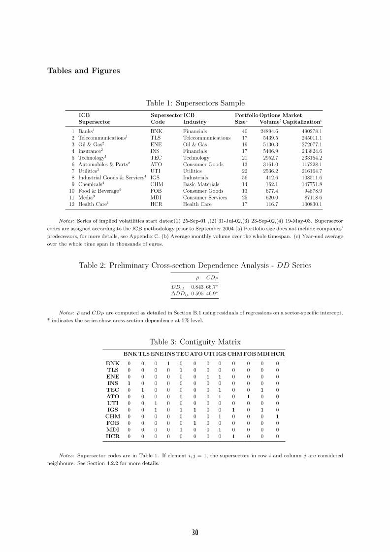
Tables and Figures
Table 1: Supersectors Sample
ICB Supersector ICB Portfolio Options MarketSupersector Code Industry Sizea Volumeb Capitalizationc
1 Banks1 BNK Financials 40 24894.6 490278.12 Telecommunications1 TLS Telecommunications 17 5439.5 245011.13 Oil & Gas2 ENE Oil & Gas 19 5130.3 272077.14 Insurance2 INS Financials 17 5406.9 233824.65 Technology1 TEC Technology 21 2952.7 233154.26 Automobiles & Parts2 ATO Consumer Goods 13 3161.0 117228.17 Utilities3 UTI Utilities 22 2536.2 216164.78 Industrial Goods & Services4 IGS Industrials 56 412.6 108511.69 Chemicals4 CHM Basic Materials 14 162.1 147751.8
10 Food & Beverage4 FOB Consumer Goods 13 677.4 94878.911 Media3 MDI Consumer Services 25 620.0 87118.612 Health Care1 HCR Health Care 17 116.7 100830.1
Notes: Series of implied volatilities start dates:(1) 25-Sep-01 ,(2) 31-Jul-02,(3) 23-Sep-02,(4) 19-May-03. Supersector
codes are assigned according to the ICB methodology prior to September 2004.(a) Portfolio size does not include companies’
predecessors, for more details, see Appendix C. (b) Average monthly volume over the whole timespan. (c) Year-end average
over the whole time span in thousands of euros.
Table 2: Preliminary Cross-section Dependence Analysis - DD Series
ρ CDP
DDi,t 0.843 66.7*∆DDi,t 0.595 46.9*
Notes: ρ and CDP are computed as detailed in Section B.1 using residuals of regressions on a sector-specific intercept.
* indicates the series show cross-section dependence at 5% level.
Table 3: Contiguity Matrix
BNK TLS ENE INS TEC ATO UTI IGS CHM FOB MDI HCR
BNK 0 0 0 1 0 0 0 0 0 0 0 0TLS 0 0 0 0 1 0 0 0 0 0 0 0ENE 0 0 0 0 0 0 1 1 0 0 0 0INS 1 0 0 0 0 0 0 0 0 0 0 0TEC 0 1 0 0 0 0 0 1 0 0 1 0ATO 0 0 0 0 0 0 0 1 0 1 0 0UTI 0 0 1 0 0 0 0 0 0 0 0 0IGS 0 0 1 0 1 1 0 0 1 0 1 0
CHM 0 0 0 0 0 0 0 1 0 0 0 1FOB 0 0 0 0 0 1 0 0 0 0 0 0MDI 0 0 0 0 1 0 0 1 0 0 0 0HCR 0 0 0 0 0 0 0 0 1 0 0 0
Notes: Supersector codes are in Table 1. If element i, j = 1, the supersectors in row i and column j are considered
neighbours. See Section 4.2.2 for more details.
30

Table 4: Residual Cross-section Dependence of ADF(p) Regressions
Average cross-correlation (ρ)
ADF(0) ADF(1) ADF(2) ADF(3) ADF(4) ADF(5) ADF(6)
DDi,t 0.605 0.603 0.608 0.608 0.610 0.610 0.596∆DYi,t 0.383 0.350 0.352 0.348 0.346 0.342 0.322∆PEi,t 0.030 0.023 0.024 0.021 0.040 0.036 0.034EXRETi,t -0.046 -0.045 -0.040 -0.039 -0.040 -0.038 -0.039ROAi,t 0.266 0.267 0.266 0.265 0.266 0.264 0.246
DDn
i,t 0.716 0.715 0.719 0.718 0.719 0.720 0.710
Pesaran test (CDP )
ADF(0) ADF(1) ADF(2) ADF(3) ADF(4) ADF(5) ADF(6)
DDi,t 47.6* 47.2* 47.4* 47.1* 47.0* 46.7* 45.4*∆DYi,t 27.6* 25.1* 25.3* 25.0* 24.9* 24.6* 23.2*∆PEi,t 2.2* 1.7* 1.8* 1.5 2.9* 2.6* 2.4*EXRETi,t -3.6* -3.5* -3.1* -3.0* -3.1* -2.9* -3.0*ROAi,t 20.9* 20.9* 20.7* 20.5* 20.5* 20.2* 18.7*
DDn
i,t 56.4* 56.0* 56.0* 55.6* 55.4* 55.2* 54.1*
Notes: pth-order Augmented Dickey Fuller ADF(p) regressions are computed for each Supersector i without cross-
section augmentations and for lag orders p = 0, . . . , 6 over the whole sample. Tests for ∆DYi,t and ∆PEi,t are based on
a reduced sample N = 11, excluding the Oil & Gas Supersector due to short series length. No linear trend is included. *
indicates rejection of the the null hypothesis of no error cross-sectional dependence at 5% level.
Table 5: Panel Unit Root Tests
CIPS Panel Unit Root Tests
CADF(0) CADF(1) CADF(2) CADF(3) CADF(4) CADF(5) CADF(6)
DDi,t -3.49*** -3.41*** -2.92*** -2.77*** -2.62*** -2.66*** -2.44***∆DYi,t -2.19* -2.29** -2.73*** -2.79*** -2.77*** -2.61*** -2.59***∆PEi,t -4.29*** -3.32*** -2.83*** -3.19*** -2.81*** -2.56*** -2.51***EXRETi,t -6.18*** -6.06*** -5.00*** -4.57*** -4.31*** -4.14*** -3.90***ROAi,t -1.49 -1.75 -1.90 -2.24** -2.31** -2.36** -2.28**
DDn
i,t -3.65*** -2.29*** -2.73*** -2.79*** -2.77*** -2.61*** -2.59***
IPS Panel Unit Root Tests
ADF(0) ADF(1) ADF(2) ADF(3) ADF(4) ADF(5) ADF(6)
DDi,t -1.34* -1.68** -0.80 -0.66 -0.40 -0.55 -0.45∆DYi,t -0.43 -2.29*** -3.91*** -4.39*** -3.82*** -4.11*** -5.94***∆PEi,t -9.97*** -6.39*** -4.8*** -5.96*** -4.84*** -4.26*** -4.81***EXRETi,t -25.76*** -20.4*** -14.62*** -12.03*** -11.35*** -10.69*** -10.06***ROAi,t 1.79 1.38 1.23 -0.09 -0.26 -0.26 -1.87***
DDn
i,t -1.05 -1.39* -0.47 -0.33 -0.14 -0.18 -0.14
Notes: Tests for ∆DYi,t and ∆PEi,t are based on a reduced sample N = 11, excluding the Oil & Gas Supersector
due to short series length. No linear trend is included. ***,**,* indicate rejection of the the null hypothesis of unit root
at 1%, 5% and 10% levels, respectively.
31

Table 6: Unit Root Tests - Macroeconomic and Financial Risk Variables
Variable Level FirstDifference
V IXt -2.07 -7.78***R3Mt -1.73 -3.92***OILt -2.11 -6.09***∆PIt -2.79* -2.60*∆CPt -6.00*** -4.77***
Notes: Intercept included only in levels, lag length determined by AIC and HQ criteria. ***,**,* indicate rejection
of the the null hypothesis of unit root at 1%, 5% and 10% levels, respectively. Results are robust to inclusion of trend and
seasonal dummies; and also to structural breaks in two cases (∆PIt, ∆CPt).
Table 7: Estimation Results
Dependent Variable MG MG MG CCEMG CCEMG CCEMG AMGDDi,t [1] [2] [3] [4] [5] [6] [7]
Intercept 0.481** 0.701** 0.487** -0.058 0.024 -0.128 5.403**(0.068) (0.134) (0.206) (0.136) (0.164) (0.156) (0.222)
∆V IXt -0.083** -0.083** -0.085** -0.000 -0.004 -0.004 0.001(0.005) (0.005) (0.006) (0.004) (0.004) (0.004) (0.007)
∆R3Mt 0.670** 0.691** 0.678** -0.010 -0.038 -0.066 0.024(0.103) (0.101) (0.103) (0.095) (0.088) (0.088) (0.119)
∆OILt -0.004 -0.006 -0.007* 0.000 -0.002 -0.003 0.111**(0.004) (0.004) (0.004) (0.003) (0.003) (0.004) (0.003)
∆PIt 0.000 0.003 -0.002 -0.000 0.001 -0.001 0.094**(0.001) (0.004) (0.005) (0.003) (0.003) (0.004) (0.009)
∆CPt -0.025* -0.038 -0.011 0.014 -0.003 0.001 -0.423**(0.011) (0.026) (0.032) (0.021) (0.017) (0.017) (0.031)
∆DYi,t 0.001 0.001 -0.001 -0.001 0.001(0.001) (0.001) (0.001) (0.001) (0.002)
∆PEi,t 0.001 0.002* 0.001 0.000 0.000(0.001) (0.001) (0.001) (0.001) (0.003)
EXRETi,t 2.365** 2.275** 2.145** 2.235** 3.118**(0.486) (0.478) (0.455) (0.485) (0.626)
∆ROAi,t 0.175** 0.241* 0.079 0.079 0.062(0.072) (0.133) (0.064) (0.069) (0.045)
DDi,t−1 0.921** 0.883** 0.767** 0.740** 0.668** 0.652** 0.417**(0.008) (0.019) (0.035) (0.042) (0.046) (0.047) (0.076)
DDn
i,t−1 0.141** 0.050 -0.479**(0.035) (0.037) (0.088)
Observations 1128 1072 1072 1128 1072 1072 1072RMSE 0.562 0.507 0.496 0.360 0.328 0.323 0.438ρ 0.424 0.429 0.424 -0.082 -0.080 -0.078 -0.034CDP 33.40‡ 37.78‡ 31.50‡ -6.48‡ -6.07‡ -5.89‡ -2.51AR(1) 7.396† 5.482† 7.044† 1.370 2.129 2.188 13.128†
Notes: MG, CCEMG and AUG stand for Mean Group (Pesaran and Smith, 1995), Common Correlated Effects Mean
Group (Pesaran, 2006) and and the Augmented Mean Group (Eberhardt and Teal, 2010; Eberhardt and Bond, 2009)
estimates respectively. Standard errors are given in parenthesis. *,** denotes significance at 10% and 5%, respectively.
CD statistics (ρ and CDP ) and panel unit root tests are computed on residuals of each equation. See Appendix B.1 for
definitions of the cross-section dependence tests. ‡ indicates rejection of the null hypothesis of cross-section independence
at 5% significance level. † indicates rejection of the null of no first-order autocorrelation test described in Drukker (2003).
32

Table 8: CCE Estimates of all Cross Section UnitsICB Supersector
DDi,t BNK TLS ENE(a) INS TEC ATO UTI IGS CHM FOB MDI HCR
Intercept -1.007** 0.175 -0.206 -0.444 -0.095 -0.726** -0.394 0.071 -0.213 0.497 -0.227 1.035**(0.480) (0.346) (0.642) (0.367) (0.213) (0.396) (0.466) (0.318) (0.381) (0.451) (0.274) (0.456)
∆V IXt 0.010 -0.005 -0.01 0.003 -0.006 -0.033** -0.023 0.029** -0.006 0.003 0.000 -0.004(0.018) (0.013) (0.013) (0.012) (0.011) (0.016) (0.018) (0.014) (0.014) (0.018) (0.012) (0.014)
∆R3Mt 0.000 0.307 0.000 0.000 -0.022 0.099 0.484 -0.466 0.263 -0.106 -0.502* 0.305(0.000) (0.301) (0.000) (0.000) (0.250) (0.366) (0.431) (0.313) (0.334) (0.43) (0.284) (0.324)
∆OILt -0.006 0.01 0.000 -0.015 0.011 -0.010 -0.020 0.005 0.021 -0.022 -0.005 0.000(0.013) (0.01) (0.000) (0.010) (0.009) (0.013) (0.015) (0.011) (0.012) (0.015) (0.010) (0.011)
∆PIt 0.017 -0.027** -0.012 0.016 -0.005 -0.008 0.000 0.009 -0.001 -0.009 0.001 0.004(0.014) (0.014) (0.020) (0.015) (0.009) (0.015) (0.000) (0.014) (0.013) (0.018) (0.010) (0.012)
∆CPt 0.000 0.000 0.038 0.018 0.002 0.140 0.115 -0.052 0.000 0.105 -0.004 0.000(0.000) (0.000) (0.111) (0.067) (0.066) (0.103) (0.118) (0.076) (0.000) (0.115) (0.069) (0.000)
∆DYi,t 0.002 0.002* -0.001 -0.003 0.001 -0.001 -0.001 -0.003 -0.002 0.000 0.003* -0.004(0.004) (0.001) (0.003) (0.002) (0.003) (0.002) (0.005) (0.004) (0.007) (0.004) (0.002) (0.004)
∆PEi,t 0.003 0.001 0.004 0.000 0.000 0.000 -0.009 0.001 0.000 0.008** 0.000 0.000(0.003) (0.001) (0.007) (0.000) (0.000) (0.000) (0.007) (0.000) (0.003) (0.004) (0.001) (0.001)
EXRETi,t 0.812 4.341** 3.090** -0.793 1.732** 3.488** 4.813** 2.777 1.136 0.907 1.029 3.486**(1.771) (1.205) (1.537) (1.238) (0.803) (1.336) (2.266) (1.779) (1.935) (1.895) (1.396) (1.369)
∆ROAi,t 0.758 -0.019 0.010 -0.226 0.007 -0.069 0.126 0.104 0.048 0.231** 0.003 -0.021(2.002) (0.042) (0.123) (0.414) (0.044) (0.190) (0.245) (0.098) (0.056) (0.101) (0.038) (0.029)
DDi,t−1 0.519** 0.484** 0.728** 0.640** 0.837** 0.399** 0.711** 0.843** 0.423** 0.736** 0.843** 0.664**(0.112) (0.103) (0.111) (0.088) (0.061) (0.123) (0.092) (0.122) (0.111) (0.09) (0.055) (0.104)
DDn
i,t−1 0.033 0.199* -0.216 0.033 0.134 0.054 0.108 0.005 -0.025 0.023 0.296** -0.040(0.133) (0.116) (0.232) (0.077) (0.142) (0.091) (0.119) (0.371) (0.124) (0.136) (0.15) (0.098)
Notes: Individual estimates come from model [6] in Table 7. *,** denotes significance at 10% and 5%, respectively.
Figure 1: Sectoral Distance-to-Default Series. December-2001 - October-2009
0
500
1000
1500
2000
2500
3000
3500
4000
4500
5000
0
1
2
3
4
5
6
7
8
9
10
11
12/0
1
06/0
2
12/0
2
06/0
3
12/0
3
06/0
4
12/0
4
06/0
5
12/0
5
06/0
6
12/0
6
06/0
7
12/0
7
06/0
8
12/0
8
06/0
9
BNK TLS ENEINS TEC ATOUTI IGS CHMFOB MDI HCREURO STOXX 50 (right)
Source. Author’s calculations.
33
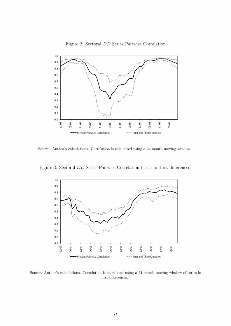
Figure 2: Sectoral DD Series Pairwise Correlation
0.0
0.1
0.2
0.3
0.4
0.5
0.6
0.7
0.8
0.9
1.011
/03
05/0
4
11/0
4
05/0
5
11/0
5
05/0
6
11/0
6
05/0
7
11/0
7
05/0
8
11/0
8
05/0
9
Median Pairwise Correlation First and Third Quartiles
Source. Author’s calculations. Correlation is calculated using a 24-month moving window.
Figure 3: Sectoral DD Series Pairwise Correlation (series in first differences)
0.0
0.1
0.2
0.3
0.4
0.5
0.6
0.7
0.8
0.9
1.0
12/0
3
06/0
4
12/0
4
06/0
5
12/0
5
06/0
6
12/0
6
06/0
7
12/0
7
06/0
8
12/0
8
06/0
9
Median Pairwise Correlation First and Third Quartiles
Source. Author’s calculations. Correlation is calculated using a 24-month moving window of series infirst differences.
34
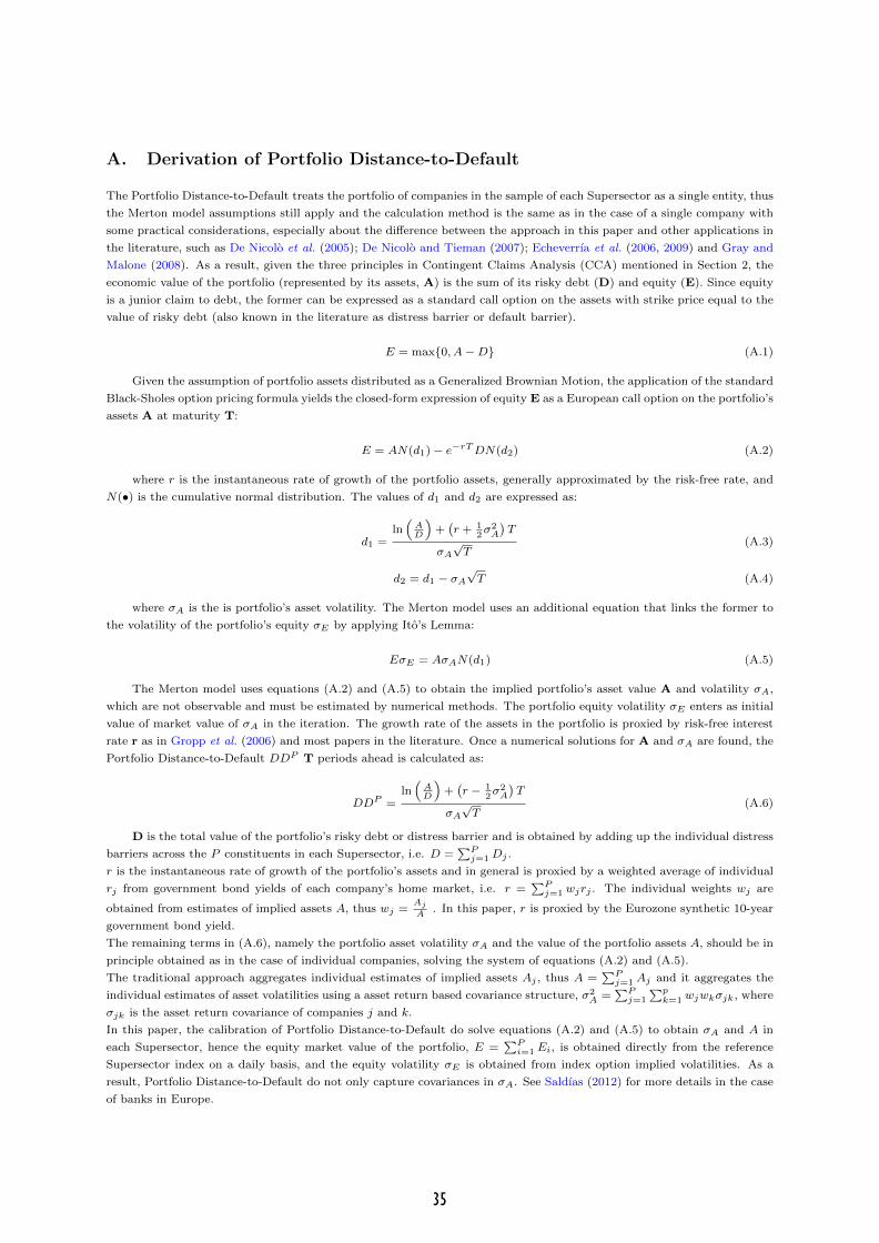
A. Derivation of Portfolio Distance-to-Default
The Portfolio Distance-to-Default treats the portfolio of companies in the sample of each Supersector as a single entity, thus
the Merton model assumptions still apply and the calculation method is the same as in the case of a single company with
some practical considerations, especially about the difference between the approach in this paper and other applications in
the literature, such as De Nicolo et al. (2005); De Nicolo and Tieman (2007); Echeverrıa et al. (2006, 2009) and Gray and
Malone (2008). As a result, given the three principles in Contingent Claims Analysis (CCA) mentioned in Section 2, the
economic value of the portfolio (represented by its assets, A) is the sum of its risky debt (D) and equity (E). Since equity
is a junior claim to debt, the former can be expressed as a standard call option on the assets with strike price equal to the
value of risky debt (also known in the literature as distress barrier or default barrier).
E = max{0, A−D} (A.1)
Given the assumption of portfolio assets distributed as a Generalized Brownian Motion, the application of the standard
Black-Sholes option pricing formula yields the closed-form expression of equity E as a European call option on the portfolio’s
assets A at maturity T:
E = AN(d1)− e−rTDN(d2) (A.2)
where r is the instantaneous rate of growth of the portfolio assets, generally approximated by the risk-free rate, and
N(•) is the cumulative normal distribution. The values of d1 and d2 are expressed as:
d1 =ln(
AD
)+(r + 1
2σ2A
)T
σA√T
(A.3)
d2 = d1 − σA√T (A.4)
where σA is the is portfolio’s asset volatility. The Merton model uses an additional equation that links the former to
the volatility of the portfolio’s equity σE by applying Ito’s Lemma:
EσE = AσAN(d1) (A.5)
The Merton model uses equations (A.2) and (A.5) to obtain the implied portfolio’s asset value A and volatility σA,
which are not observable and must be estimated by numerical methods. The portfolio equity volatility σE enters as initial
value of market value of σA in the iteration. The growth rate of the assets in the portfolio is proxied by risk-free interest
rate r as in Gropp et al. (2006) and most papers in the literature. Once a numerical solutions for A and σA are found, the
Portfolio Distance-to-Default DDP T periods ahead is calculated as:
DDP =ln(
AD
)+(r − 1
2σ2A
)T
σA√T
(A.6)
D is the total value of the portfolio’s risky debt or distress barrier and is obtained by adding up the individual distress
barriers across the P constituents in each Supersector, i.e. D =∑P
j=1Dj .
r is the instantaneous rate of growth of the portfolio’s assets and in general is proxied by a weighted average of individual
rj from government bond yields of each company’s home market, i.e. r =∑P
j=1 wjrj . The individual weights wj are
obtained from estimates of implied assets A, thus wj =Aj
A. In this paper, r is proxied by the Eurozone synthetic 10-year
government bond yield.
The remaining terms in (A.6), namely the portfolio asset volatility σA and the value of the portfolio assets A, should be in
principle obtained as in the case of individual companies, solving the system of equations (A.2) and (A.5).
The traditional approach aggregates individual estimates of implied assets Aj , thus A =∑P
j=1 Aj and it aggregates the
individual estimates of asset volatilities using a asset return based covariance structure, σ2A =
∑Pj=1
∑pk=1 wjwkσjk, where
σjk is the asset return covariance of companies j and k.
In this paper, the calibration of Portfolio Distance-to-Default do solve equations (A.2) and (A.5) to obtain σA and A in
each Supersector, hence the equity market value of the portfolio, E =∑P
i=1 Ei, is obtained directly from the reference
Supersector index on a daily basis, and the equity volatility σE is obtained from index option implied volatilities. As a
result, Portfolio Distance-to-Default do not only capture covariances in σA. See Saldıas (2012) for more details in the case
of banks in Europe.
35

B. Cross-section Dependence and Panel Unit Root tests
B.1. Cross-section Dependence Tests
The two statistics of cross-section dependence (CD) in panel data used in the paper are based on pairwise correlation
coefficients, ρij , of regressions’ residuals23. The average of cross-correlation coefficients, ρ, is applied to provide a
first assessment at a descriptive level.
ρ =1
N(N − 1)
N−1∑i=1
N−1∑j=i+1
ρij (B.1)
The Pesaran CD statistic, CDP , was developed in Pesaran (2004) and is used for panels where series may be either
stationary or contain unit roots. This CD statistic shows good properties with dynamic panels but has also a caveat. Since
it involves the sum of pairwise correlation coefficients instead of the sum of squared correlations, the CDP statistic might
miss out CD where there are alternating signs of correlations in the residuals. This statistic takes the following form and
distribution.
CDP =
√2T
N(N − 1)
N−1∑i=1
N∑j=i+1
ρijd→ N(0, 1) (B.2)
B.2. Unit Root Tests
In addition to the IPS test, cross-sectionally augmented IPS tests (CIPS) (Pesaran, 2007) are applied. This test
allows for individual unit root processes and for different serial correlation properties across units. It is more suitable in
the presence of cross-section dependence in the series, since IPS may lead to spurious inference. The CIPS test statistic
is computed using the average of the individual pth order cross-sectionally Augmented Dickey-Fuller (ADF) regressions’
statistics (CADF). It assumes a single unobserved common factor, but is robust to other potential sources of CD, such as
spill-over effects (Baltagi et al., 2007). This assumed factor structure is accounted for by adding the averages of lagged
levels and first-differences of the dependent variable to each standard ADF regression.
∆yi,t = ai + biyi,t−1 +
pi∑l=1
ci,l∆yi,t−l + d′izt + νi,t, i = 1, . . . , N ; t = 1, . . . , T (B.3)
where zt = (yt−1,∆yt,∆yt−1, . . . ,∆yt−p)′. The joint asymptotic limit of the CIPS statistic is nonstandard and critical
values can be found in Pesaran (2007) for various numbers of cross-section units N and time series lengths T . Under the
null hypothesis of non-stationarity against the possibly heterogeneous presence of unit roots across i, the CIPS statistic
takes the following form.
CIPS =1
N
N∑i=1
ti (B.4)
where ti is the t-statistic associated to bi in CADF equations.
23ρij = ρji =∑T
t=1 uitujt√∑Tt=1 u2
it
√∑Tt=1 u2
jt
, where uit and ujt are residuals from equation (1) or individual
series’ ADF(p) or cross-sectionally augmented ADF(p) regressions, CADF(p).
36
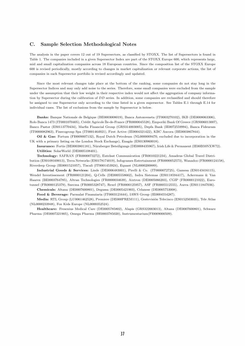
C. Sample Selection Methodological Notes
The analysis in the paper covers 12 out of 19 Supersectors, as classified by STOXX. The list of Supersectors is found in
Table 1. The companies included in a given Supersector Index are part of the STOXX Europe 600, which represents large,
mid and small capitalization companies across 18 European countries. Since the composition list of the STOXX Europe
600 is revised periodically, mostly according to changes in market capitalization or relevant corporate actions, the list of
companies in each Supersector portfolio is revised accordingly and updated.
Since the most relevant changes take place at the bottom of the ranking, some companies do not stay long in the
Supersector Indices and may only add noise to the series. Therefore, some small companies were excluded from the sample
under the assumption that their low weight in their respective index would not affect the aggregation of company informa-
tion by Supersector during the calibration of DD series. In addition, some companies are reclassified and should therefore
be assigned to one Supersector only according to the time listed in a given supersector. See Tables E.1 through E.14 for
individual cases. The list of exclusions from the sample by Supersector is below.
Banks: Banque Nationale de Belgique (BE0003008019), Banca Antonveneta (IT0003270102), IKB (DE0008063306),
Rolo Banca 1473 (IT0001070405), Credit Agricole Ile-de-France (FR0000045528), Emporiki Bank Of Greece (GRS006013007),
Banco Pastor (ES0113770434), Marfin Financial Group (GRS314003005), Depfa Bank (IE0072559994), Banca Fideuram
(IT0000082963), Finecogroup Spa (IT0001464921), First Active (IE0004321422), KBC Ancora (BE0003867844).
Oil & Gas: Fortum (FI0009007132), Royal Dutch Petroleum (NL0000009470, excluded due to incorporation in the
UK with a primary listing on the London Stock Exchange), Enagas (ES0130960018).
Insurance: Fortis (BE0003801181), Nurnberger Beteiligungs (DE0008435967), Irish Life & Permanent (IE00B59NXW72).
Utilities: SolarWorld (DE0005108401).
Technology: SAFRAN (FR0000073272), Eutelsat Communication (FR0010221234), Amadeus Global Travel Distri-
bution (ES0109169013), Terra Networks (ES0178174019), Infogrames Entertainment (FR0000052573), Wanadoo (FR0000124158),
Riverdeep Group (IE0001521057), Tiscali (IT0001453924), Equant (NL0000200889).
Industrial Goods & Services: Linde (DE0006483001), Pirelli & Co. (IT0000072725), Gamesa (ES0143416115),
Wendel Investissement (FR0000121204), Q-Cells (DE0005558662), Indra Sistemas (ES0118594417), Ackermans & Van
Haaren (BE0003764785), Altran Technologies (FR0000034639), Aixtron (DE0005066203), CGIP (FR0000121022), Euro-
tunnel (FR0000125379), Snecma (FR0005328747), Rexel (FR0000125957), ASF (FR0005512555), Aurea (ES0111847036).
Chemicals: Altana (DE0007600801), Degussa (DE0005421903), Celanese (DE0005753008).
Food & Beverage: Parmalat Finanziaria (IT0003121644), IAWS Group (IE0004554287).
Media: RTL Group (LU0061462528), Premiere (DE000PREM111), Gestevision Telecinco (ES0152503035), Tele Atlas
(NL0000233948), Fox Kids Europe (NL0000352524).
Healthcare: Fresenius Medical Care (DE0005785802), Alapis (GRS322003013), Altana (DE0007600801), Schwarz
Pharma (DE0007221905), Omega Pharma (BE0003785020), Instrumentarium(FI0009000509).
37
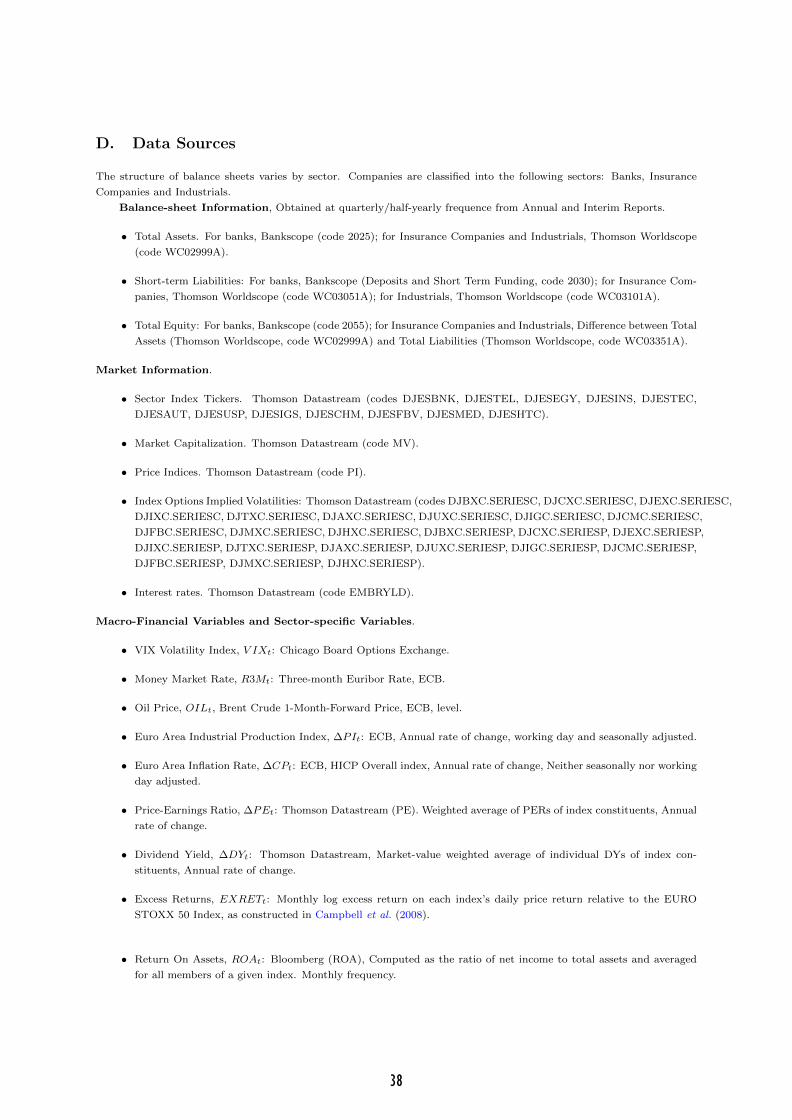
D. Data Sources
The structure of balance sheets varies by sector. Companies are classified into the following sectors: Banks, Insurance
Companies and Industrials.
Balance-sheet Information, Obtained at quarterly/half-yearly frequence from Annual and Interim Reports.
• Total Assets. For banks, Bankscope (code 2025); for Insurance Companies and Industrials, Thomson Worldscope
(code WC02999A).
• Short-term Liabilities: For banks, Bankscope (Deposits and Short Term Funding, code 2030); for Insurance Com-
panies, Thomson Worldscope (code WC03051A); for Industrials, Thomson Worldscope (code WC03101A).
• Total Equity: For banks, Bankscope (code 2055); for Insurance Companies and Industrials, Difference between Total
Assets (Thomson Worldscope, code WC02999A) and Total Liabilities (Thomson Worldscope, code WC03351A).
Market Information.
• Sector Index Tickers. Thomson Datastream (codes DJESBNK, DJESTEL, DJESEGY, DJESINS, DJESTEC,
DJESAUT, DJESUSP, DJESIGS, DJESCHM, DJESFBV, DJESMED, DJESHTC).
• Market Capitalization. Thomson Datastream (code MV).
• Price Indices. Thomson Datastream (code PI).
• Index Options Implied Volatilities: Thomson Datastream (codes DJBXC.SERIESC, DJCXC.SERIESC, DJEXC.SERIESC,
DJIXC.SERIESC, DJTXC.SERIESC, DJAXC.SERIESC, DJUXC.SERIESC, DJIGC.SERIESC, DJCMC.SERIESC,
DJFBC.SERIESC, DJMXC.SERIESC, DJHXC.SERIESC, DJBXC.SERIESP, DJCXC.SERIESP, DJEXC.SERIESP,
DJIXC.SERIESP, DJTXC.SERIESP, DJAXC.SERIESP, DJUXC.SERIESP, DJIGC.SERIESP, DJCMC.SERIESP,
DJFBC.SERIESP, DJMXC.SERIESP, DJHXC.SERIESP).
• Interest rates. Thomson Datastream (code EMBRYLD).
Macro-Financial Variables and Sector-specific Variables.
• VIX Volatility Index, V IXt: Chicago Board Options Exchange.
• Money Market Rate, R3Mt: Three-month Euribor Rate, ECB.
• Oil Price, OILt, Brent Crude 1-Month-Forward Price, ECB, level.
• Euro Area Industrial Production Index, ∆PIt: ECB, Annual rate of change, working day and seasonally adjusted.
• Euro Area Inflation Rate, ∆CPt: ECB, HICP Overall index, Annual rate of change, Neither seasonally nor working
day adjusted.
• Price-Earnings Ratio, ∆PEt: Thomson Datastream (PE). Weighted average of PERs of index constituents, Annual
rate of change.
• Dividend Yield, ∆DYt: Thomson Datastream, Market-value weighted average of individual DYs of index con-
stituents, Annual rate of change.
• Excess Returns, EXRETt: Monthly log excess return on each index’s daily price return relative to the EURO
STOXX 50 Index, as constructed in Campbell et al. (2008).
• Return On Assets, ROAt: Bloomberg (ROA), Computed as the ratio of net income to total assets and averaged
for all members of a given index. Monthly frequency.
38

E. Constituents by Supersector
Table E.1: Supersector Constituents List - Banks (BNK)
Name ISIN Code Country Portfolio constituentfrom: to:
1 Deutsche Bank DE0005140008 DE 31-Dec-01 31-Oct-092 BNP Paribas(1) FR0000131104 FR 31-Dec-01 31-Oct-09→ Fortis(2)(3) BE0003801181 BE 31-Dec-01 21-Sep-09→ Banca Nazionale IT0001254884 IT 31-Dec-01 22-May-06
del Lavoro(2)
3 Credit Agricole FR0000045072 FR 18-Mar-02 31-Oct-09→ Credit Lyonnais(2) FR0000184202 FR 31-Dec-01 19-Jun-034 Societe Generale FR0000130809 FR 31-Dec-01 31-Oct-095 UniCredit IT0000064854 IT 31-Dec-01 31-Oct-09→ Capitalia(2)(4) IT0003121495 IT 31-Dec-01 1-Oct-07→ HypoVereinsbank(2)(5) DE0008022005 DE 31-Dec-01 19-Jun-06→ Bank Austria(2) AT0000995006 AT 24-Oct-03 5-Dec-056 Santander(6) ES0113900J37 ES 31-Dec-01 31-Oct-09→ ABN Amro(7) NL0000301109 NL 31-Dec-01 2-Nov-077 Dexia(8) BE0003796134 BE 31-Dec-01 31-Oct-098 Commerzbank(9) DE0008032004 DE 10-Aug-07 31-Oct-099 Intesa Sanpaolo(10) IT0000072618 IT 31-Dec-01 31-Oct-09→ San Paolo IMI(2) IT0001269361 IT 31-Dec-01 2-Jan-0710 Natixis FR0000120685 FR 19-Apr-05 31-Oct-0911 BBVA ES0113211835 ES 31-Dec-01 31-Oct-0912 KBC BE0003565737 BE 31-Dec-01 31-Oct-09→ Almanij(2) BE0003703171 BE 31-Dec-01 3-Mar-0513 Deutsche Postbank DE0008001009 DE 20-Sep-04 31-Oct-0914 Erste Group Bank(11) AT0000652011 AT 31-Dec-01 31-Oct-0915 Bank Of Ireland IE0030606259 IE 31-Dec-01 31-Oct-0916 Banca Monte dei IT0001334587 IT 31-Dec-01 31-Oct-09
Paschi di Siena(12)
17 Allied Irish Banks IE0000197834 IE 31-Dec-01 31-Oct-09
Notes: (1) Increase in share capital and free float change on 19-May-09. (2) Takeover. (3) Also constituent prior to 21-Jun-04. (4)
Formerly Banca di Roma. (5) Also constituent between 24-Nov-05 and 19-Jun-06 after takeover. (6) Increase in share capital due to takeover
of Abbey on 16-Nov-04. (7) Takeover by Royal Bank of Scotland, Fortis and Santander. (8) Increase in share capital on 8-Jan-09. (9) Increase
in share capital on 23-Jul-09. (10) Banca Intesa is the predecessor company. Increase in free float on 19-Apr-04. (11) Increase in share capital
on 31-Jan-06. (12) Increase in share capital due to takeover of Banca Agricola Mantovana and Banca Toscana on 31-Mar-03.
39
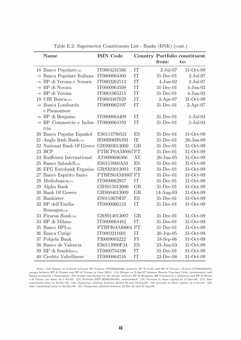
Table E.2: Supersector Constituents List - Banks (BNK) (cont.)
Name ISIN Code Country Portfolio constituentfrom: to:
18 Banco Popolare(13) IT0004231566 IT 2-Jul-07 31-Oct-09→ Banca Popolare Italiana IT0000064300 IT 31-Dec-01 2-Jul-07→ BP di Verona e Novara IT0003262513 IT 4-Jun-02 2-Jul-07→ BP di Novara IT0000064508 IT 31-Dec-01 4-Jun-02→ BP di Verona IT0001065215 IT 31-Dec-01 4-Jun-0219 UBI Banca(14) IT0003487029 IT 2-Apr-07 31-Oct-09→ Banca Lombarda IT0000062197 IT 31-Dec-01 2-Apr-07
e Piemontese→ BP di Bergamo IT0000064409 IT 31-Dec-01 1-Jul-03→ BP Commercio e Indus-
triaIT0000064193 IT 31-Dec-01 1-Jul-03
20 Banco Popular Espanol ES0113790531 ES 31-Dec-01 31-Oct-0921 Anglo Irish Bank(15) IE00B06H8J93 IE 31-Dec-01 26-Jan-0922 National Bank Of Greece GRS003013000 GR 31-Dec-01 31-Oct-0923 BCP PTBCP0AM0007PT 31-Dec-01 31-Oct-0924 Raiffeisen International AT0000606306 AT 20-Jun-05 31-Oct-0925 Banco Sabadell(16) ES0113860A34 ES 31-Dec-01 31-Oct-0926 EFG Eurobank Ergasias GRS323013003 GR 31-Dec-01 31-Oct-0927 Banco Espirito Santo PTBES0AM0007 PT 31-Dec-01 31-Oct-0928 Mediobanca(17) IT0000062957 IT 31-Dec-01 31-Oct-0929 Alpha Bank GRS015013006 GR 31-Dec-01 31-Oct-0930 Bank Of Greece GRS004013009 GR 14-Aug-03 31-Oct-0931 Bankinter ES0113679I37 ES 31-Dec-01 31-Oct-0932 BP dell’Emilia IT0000066123 IT 31-Dec-01 31-Oct-09
Romagna(18)
33 Piraeus Bank(19) GRS014013007 GR 31-Dec-01 31-Oct-0934 BP di Milano IT0000064482 IT 31-Dec-01 31-Oct-0935 Banco BPI(20) PTBPI0AM0004 PT 31-Dec-01 31-Oct-0936 Banca Carige IT0003211601 IT 20-Jun-05 31-Oct-0937 Pohjola Bank FI0009003222 FI 18-Sep-06 31-Oct-0938 Banco de Valencia ES0113980F34 ES 23-Jun-03 31-Oct-0939 BP di Sondrio(21) IT0000784196 IT 31-Dec-01 31-Oct-0940 Credito Valtellinese IT0000064516 IT 22-Dec-08 31-Oct-09
Notes: (13) Merger on 2-Jul-07 between BP Italiana (IT0000064300, formerly BP di Lodi) and BP di Verona e Novara (IT0003262513,
merger between BP di Novara and BP di Verona in June 2002). (14) Merger on 2-Apr-07 between Banche Popolare Unite (predecessor) and
Banca Lombarda e Piamontese. The former was formed by the merger between BP di Bergamo, BP Commercio e Industria and BP di Ruino
e di Varese (no data) on 1-Jul-03. (15) Previous ISIN IE0001987894, nationalized. (16) Increase in share capital on 15-Mar-04. (17) Also
constituent prior to 23-Dec-02. (18) Temporary deletion between 22-Dec-03 and 10-Sep-09. (19) Increase in share capital on 2-Jan-04. (20)
Also constituent prior to 24-Mar-03. (21) Temporary deletion between 22-Dec-03 and 21-Sep-09.
40
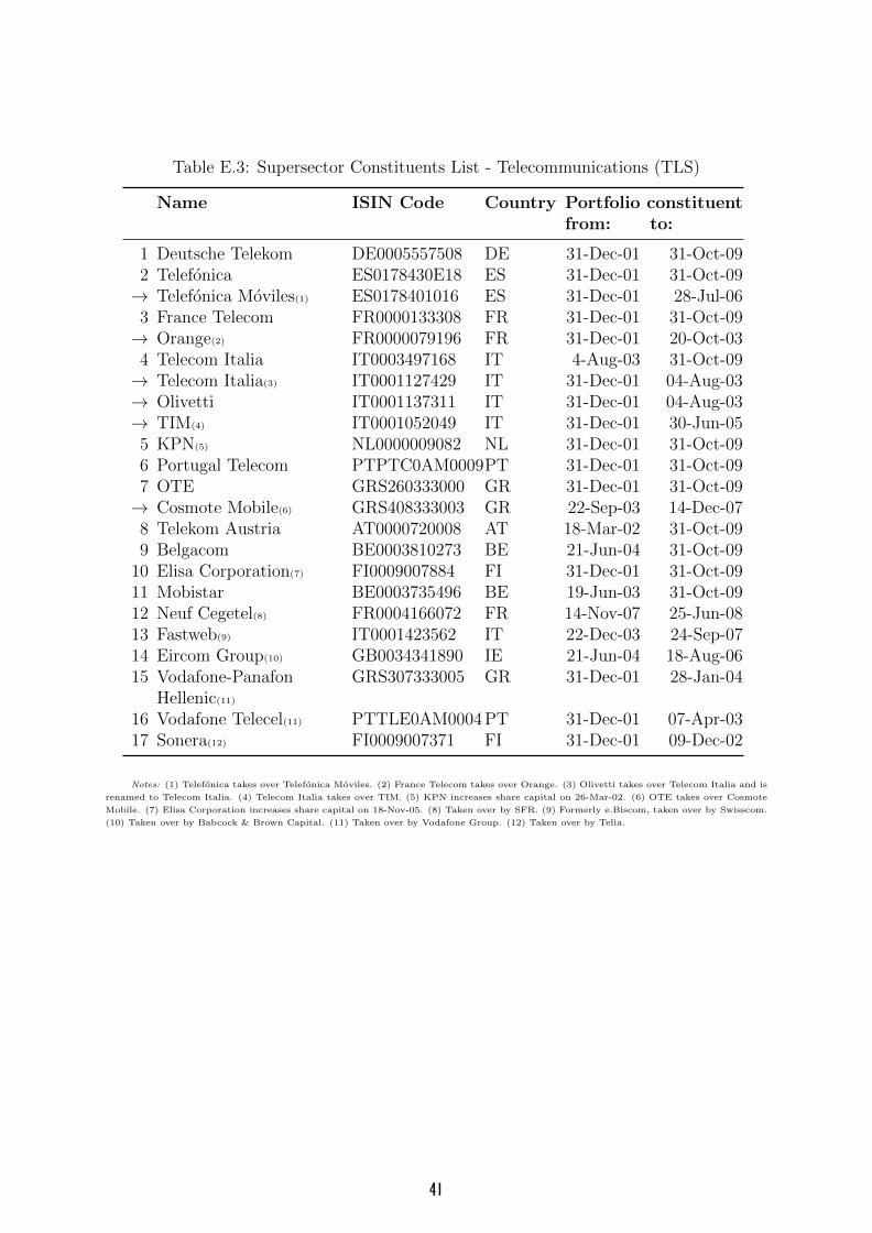
Table E.3: Supersector Constituents List - Telecommunications (TLS)
Name ISIN Code Country Portfolio constituentfrom: to:
1 Deutsche Telekom DE0005557508 DE 31-Dec-01 31-Oct-092 Telefonica ES0178430E18 ES 31-Dec-01 31-Oct-09→ Telefonica Moviles(1) ES0178401016 ES 31-Dec-01 28-Jul-063 France Telecom FR0000133308 FR 31-Dec-01 31-Oct-09→ Orange(2) FR0000079196 FR 31-Dec-01 20-Oct-034 Telecom Italia IT0003497168 IT 4-Aug-03 31-Oct-09→ Telecom Italia(3) IT0001127429 IT 31-Dec-01 04-Aug-03→ Olivetti IT0001137311 IT 31-Dec-01 04-Aug-03→ TIM(4) IT0001052049 IT 31-Dec-01 30-Jun-055 KPN(5) NL0000009082 NL 31-Dec-01 31-Oct-096 Portugal Telecom PTPTC0AM0009PT 31-Dec-01 31-Oct-097 OTE GRS260333000 GR 31-Dec-01 31-Oct-09→ Cosmote Mobile(6) GRS408333003 GR 22-Sep-03 14-Dec-078 Telekom Austria AT0000720008 AT 18-Mar-02 31-Oct-099 Belgacom BE0003810273 BE 21-Jun-04 31-Oct-09
10 Elisa Corporation(7) FI0009007884 FI 31-Dec-01 31-Oct-0911 Mobistar BE0003735496 BE 19-Jun-03 31-Oct-0912 Neuf Cegetel(8) FR0004166072 FR 14-Nov-07 25-Jun-0813 Fastweb(9) IT0001423562 IT 22-Dec-03 24-Sep-0714 Eircom Group(10) GB0034341890 IE 21-Jun-04 18-Aug-0615 Vodafone-Panafon GRS307333005 GR 31-Dec-01 28-Jan-04
Hellenic(11)
16 Vodafone Telecel(11) PTTLE0AM0004 PT 31-Dec-01 07-Apr-0317 Sonera(12) FI0009007371 FI 31-Dec-01 09-Dec-02
Notes: (1) Telefonica takes over Telefonica Moviles. (2) France Telecom takes over Orange. (3) Olivetti takes over Telecom Italia and is
renamed to Telecom Italia. (4) Telecom Italia takes over TIM. (5) KPN increases share capital on 26-Mar-02. (6) OTE takes over Cosmote
Mobile. (7) Elisa Corporation increases share capital on 18-Nov-05. (8) Taken over by SFR. (9) Formerly e.Biscom, taken over by Swisscom.
(10) Taken over by Babcock & Brown Capital. (11) Taken over by Vodafone Group. (12) Taken over by Telia.
41
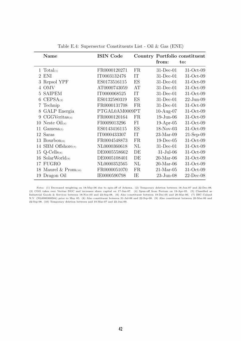
Table E.4: Supersector Constituents List - Oil & Gas (ENE)
Name ISIN Code Country Portfolio constituentfrom: to:
1 Total(1) FR0000120271 FR 31-Dec-01 31-Oct-092 ENI IT0003132476 IT 31-Dec-01 31-Oct-093 Repsol YPF ES0173516115 ES 31-Dec-01 31-Oct-094 OMV AT0000743059 AT 31-Dec-01 31-Oct-095 SAIPEM IT0000068525 IT 31-Dec-01 31-Oct-096 CEPSA(2) ES0132580319 ES 31-Dec-01 22-Jun-097 Technip FR0000131708 FR 31-Dec-01 31-Oct-098 GALP Energia PTGAL0AM0009PT 10-Aug-07 31-Oct-099 CGGVeritas(3) FR0000120164 FR 19-Jun-06 31-Oct-09
10 Neste Oil(4) FI0009013296 FI 19-Apr-05 31-Oct-0911 Gamesa(5) ES0143416115 ES 18-Nov-03 31-Oct-0912 Saras IT0000433307 IT 23-Mar-09 21-Sep-0913 Bourbon(6) FR0004548873 FR 19-Dec-05 31-Oct-0914 SBM Offshore(7) NL0000360618 NL 31-Dec-01 31-Oct-0915 Q-Cells(8) DE0005558662 DE 31-Jul-06 31-Oct-0916 SolarWorld(9) DE0005108401 DE 20-Mar-06 31-Oct-0917 FUGRO NL0000352565 NL 20-Mar-06 31-Oct-0918 Maurel & Prom(10) FR0000051070 FR 21-Mar-05 31-Oct-0919 Dragon Oil IE0000590798 IE 23-Jun-08 22-Dec-08
Notes: (1) Decreased weighting on 18-May-06 due to spin-off of Arkema. (2) Temporary deletion between 18-Jun-07 and 22-Dec-08.
(3) CGG takes over Veritas DGC and increases share capital on 17-Jan-07. (4) Spun-off from Fortum on 19-Apr-05. (5) Classified as
Industrial Goods & Services between 18-Nov-03 and 22-Sep-08. (6) Also constituent between 19-Dec-05 and 20-Mar-06. (7) IHC Caland
N.V. (NL0000360584) prior to May 05. (8) Also constituent between 31-Jul-06 and 22-Sep-08. (9) Also constituent between 20-Mar-06 and
22-Sep-08. (10) Temporary deletion between and 19-Mar-07 and 22-Jun-09.
42
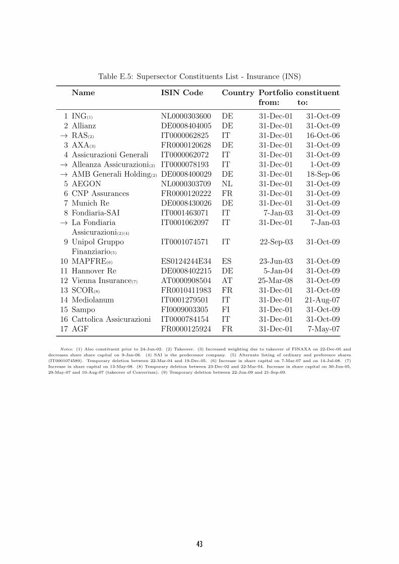
Table E.5: Supersector Constituents List - Insurance (INS)
Name ISIN Code Country Portfolio constituentfrom: to:
1 ING(1) NL0000303600 DE 31-Dec-01 31-Oct-092 Allianz DE0008404005 DE 31-Dec-01 31-Oct-09→ RAS(2) IT0000062825 IT 31-Dec-01 16-Oct-063 AXA(3) FR0000120628 DE 31-Dec-01 31-Oct-094 Assicurazioni Generali IT0000062072 IT 31-Dec-01 31-Oct-09→ Alleanza Assicurazioni(2) IT0000078193 IT 31-Dec-01 1-Oct-09→ AMB Generali Holding(2) DE0008400029 DE 31-Dec-01 18-Sep-065 AEGON NL0000303709 NL 31-Dec-01 31-Oct-096 CNP Assurances FR0000120222 FR 31-Dec-01 31-Oct-097 Munich Re DE0008430026 DE 31-Dec-01 31-Oct-098 Fondiaria-SAI IT0001463071 IT 7-Jan-03 31-Oct-09→ La Fondiaria IT0001062097 IT 31-Dec-01 7-Jan-03
Assicurazioni(2)(4)
9 Unipol Gruppo IT0001074571 IT 22-Sep-03 31-Oct-09Finanziario(5)
10 MAPFRE(6) ES0124244E34 ES 23-Jun-03 31-Oct-0911 Hannover Re DE0008402215 DE 5-Jan-04 31-Oct-0912 Vienna Insurance(7) AT0000908504 AT 25-Mar-08 31-Oct-0913 SCOR(8) FR0010411983 FR 31-Dec-01 31-Oct-0914 Mediolanum IT0001279501 IT 31-Dec-01 21-Aug-0715 Sampo FI0009003305 FI 31-Dec-01 31-Oct-0916 Cattolica Assicurazioni IT0000784154 IT 31-Dec-01 31-Oct-0917 AGF FR0000125924 FR 31-Dec-01 7-May-07
Notes: (1) Also constituent prior to 24-Jun-02. (2) Takeover. (3) Increased weighting due to takeover of FINAXA on 22-Dec-05 and
decreases share share capital on 9-Jan-06. (4) SAI is the predecessor company. (5) Alternate listing of ordinary and preference shares
(IT0001074589). Temporary deletion between 22-Mar-04 and 19-Dec-05. (6) Increase in share capital on 7-Mar-07 and on 14-Jul-08. (7)
Increase in share capital on 13-May-08. (8) Temporary deletion between 23-Dec-02 and 22-Mar-04. Increase in share capital on 30-Jun-05,
29-May-07 and 10-Aug-07 (takeover of Converium). (9) Temporary deletion between 22-Jun-09 and 21-Sep-09.
43

Table E.6: Supersector Constituents List - Technology (TEC)
Name ISIN Code Country Portfolio constituentfrom: to:
1 Nokia FI0009000681 FI 31-Dec-01 31-Oct-092 Alcatel Lucent(1) FR0000130007 FR 31-Dec-01 31-Oct-093 SAP DE0007164600 DE 31-Dec-01 31-Oct-09→ Business Objects(2) FR0004026250 FR 31-Dec-01 11-Feb-084 STMicroelectronics NL0000226223 IT 31-Dec-01 31-Oct-095 Capgemini FR0000125338 FR 31-Dec-01 31-Oct-096 Infineon Technologies DE0006231004 DE 31-Dec-01 31-Oct-097 Atos Origin(3) FR0000051732 FR 31-Dec-01 31-Oct-098 ASML Holding NL0006034001 NL 31-Dec-01 31-Oct-099 Indra Sistemas(4) ES0118594417 ES 31-Dec-01 31-Oct-09
10 Dassault Systems FR0000130650 FR 31-Dec-01 31-Oct-0911 Neopost FR0000120560 FR 24-Jun-02 31-Oct-0912 Iliad FR0004035913 FR 22-Sep-08 31-Oct-0913 Wincor Nixdorf DE000A0CAYB2 DE 19-Jun-06 31-Oct-0914 United Internet DE0005089031 DE 19-Mar-07 31-Oct-0915 Software DE0003304002 DE 23-Mar-09 31-Oct-0916 Aixtron DE000A0WMPJ6DE 21-Sep-09 31-Oct-0917 Tom Tom NL0000387058 NL 24-Sep-07 22-Dec-0818 Tietoenator FI0009000277 FI 31-Dec-01 24-Sep-0719 Getronics NL0000355915 NL 22-Mar-04 18-Sep-0620 Oce NL0000354934 NL 31-Dec-01 19-Jun-0621 T-Online International DE0005557706 DE 31-Dec-01 20-Mar-06
Notes: (1) Increase in share capital on 4-Dec-06 due to takeover of Lucent Technologies. (2) Takeover by SAP. (3) Increase in share
capital on 2-Feb-04. (4) Increase in share capital on 1-Feb-07, also constituent prior to 31-Dec-03.
44
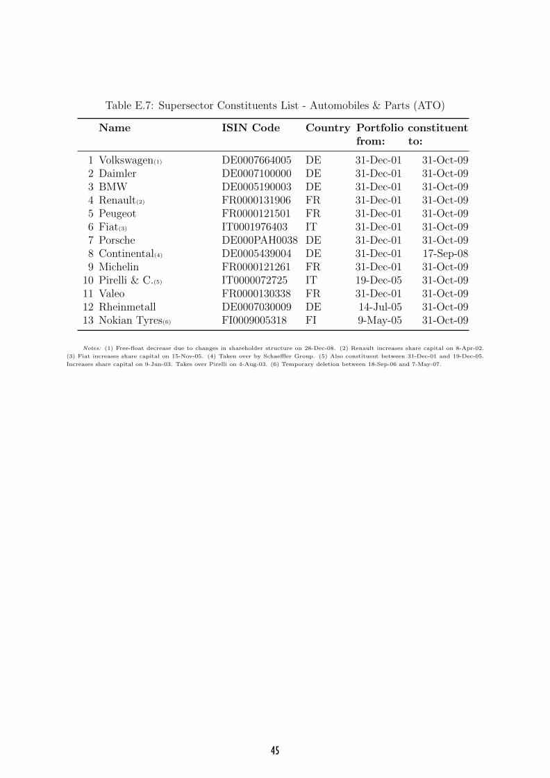
Table E.7: Supersector Constituents List - Automobiles & Parts (ATO)
Name ISIN Code Country Portfolio constituentfrom: to:
1 Volkswagen(1) DE0007664005 DE 31-Dec-01 31-Oct-092 Daimler DE0007100000 DE 31-Dec-01 31-Oct-093 BMW DE0005190003 DE 31-Dec-01 31-Oct-094 Renault(2) FR0000131906 FR 31-Dec-01 31-Oct-095 Peugeot FR0000121501 FR 31-Dec-01 31-Oct-096 Fiat(3) IT0001976403 IT 31-Dec-01 31-Oct-097 Porsche DE000PAH0038 DE 31-Dec-01 31-Oct-098 Continental(4) DE0005439004 DE 31-Dec-01 17-Sep-089 Michelin FR0000121261 FR 31-Dec-01 31-Oct-09
10 Pirelli & C.(5) IT0000072725 IT 19-Dec-05 31-Oct-0911 Valeo FR0000130338 FR 31-Dec-01 31-Oct-0912 Rheinmetall DE0007030009 DE 14-Jul-05 31-Oct-0913 Nokian Tyres(6) FI0009005318 FI 9-May-05 31-Oct-09
Notes: (1) Free-float decrease due to changes in shareholder structure on 28-Dec-08. (2) Renault increases share capital on 8-Apr-02.
(3) Fiat increases share capital on 15-Nov-05. (4) Taken over by Schaeffler Group. (5) Also constituent between 31-Dec-01 and 19-Dec-05.
Increases share capital on 9-Jun-03. Takes over Pirelli on 4-Aug-03. (6) Temporary deletion between 18-Sep-06 and 7-May-07.
45
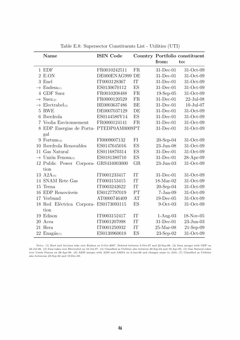
Table E.8: Supersector Constituents List - Utilities (UTI)
Name ISIN Code Country Portfolio constituentfrom: to:
1 EDF FR0010242511 FR 31-Dec-01 31-Oct-092 E.ON DE000ENAG999 DE 31-Dec-01 31-Oct-093 Enel IT0003128367 IT 31-Dec-01 31-Oct-09→ Endesa(1) ES0130670112 ES 31-Dec-01 31-Oct-094 GDF Suez FR0010208488 FR 19-Sep-05 31-Oct-09→ Suez(2) FR0000120529 FR 31-Dec-01 22-Jul-08→ Electrabel(3) BE0003637486 BE 31-Dec-01 10-Jul-075 RWE DE0007037129 DE 31-Dec-01 31-Oct-096 Iberdrola ES0144580Y14 ES 31-Dec-01 31-Oct-097 Veolia Environnement FR0000124141 FR 31-Dec-01 31-Oct-098 EDP Energias de Portu-
galPTEDP0AM0009PT 31-Dec-01 31-Oct-09
9 Fortum(4) FI0009007132 FI 20-Sep-04 31-Oct-0910 Iberdrola Renovables ES0147645016 ES 23-Jun-08 31-Oct-0911 Gas Natural ES0116870314 ES 31-Dec-01 31-Oct-09→ Union Fenosa(5) ES0181380710 ES 31-Dec-01 28-Apr-0912 Public Power Corpora-
tionGRS434003000 GR 23-Jun-03 31-Oct-09
13 A2A(6) IT0001233417 IT 31-Dec-01 31-Oct-0914 SNAM Rete Gas IT0003153415 IT 18-Mar-02 31-Oct-0915 Terna IT0003242622 IT 20-Sep-04 31-Oct-0916 EDP Renovaveis ES0127797019 PT 7-Jan-09 31-Oct-0917 Verbund AT0000746409 AT 19-Dec-05 31-Oct-0918 Red Electrica Corpora-
tionES0173093115 ES 9-Oct-03 31-Oct-09
19 Edison IT0003152417 IT 1-Aug-03 18-Nov-0520 Acea IT0001207098 IT 31-Dec-01 23-Jun-0321 Hera IT0001250932 IT 25-Mar-08 21-Sep-0922 Enagas(7) ES0130960018 ES 23-Sep-02 31-Oct-09
Notes: (1) Enel and Acciona take over Endesa on 5-Oct-2007. Deleted between 5-Oct-07 and 22-Sep-08. (2) Suez merges with GDF on
22-Jul-08. (3) Suez takes over Electrabel on 10-Jul-07. (4) Classified as Utilities also between 20-Sep-04 and 19-Apr-05. (5) Gas Natural takes
over Union Fenosa on 28-Apr-09. (6) AEM merges with ASM and AMSA on 2-Jan-08 and changes name to A2A. (7) Classified as Utilities
also betweenn 23-Sep-02 and 19-Dec-05.
46
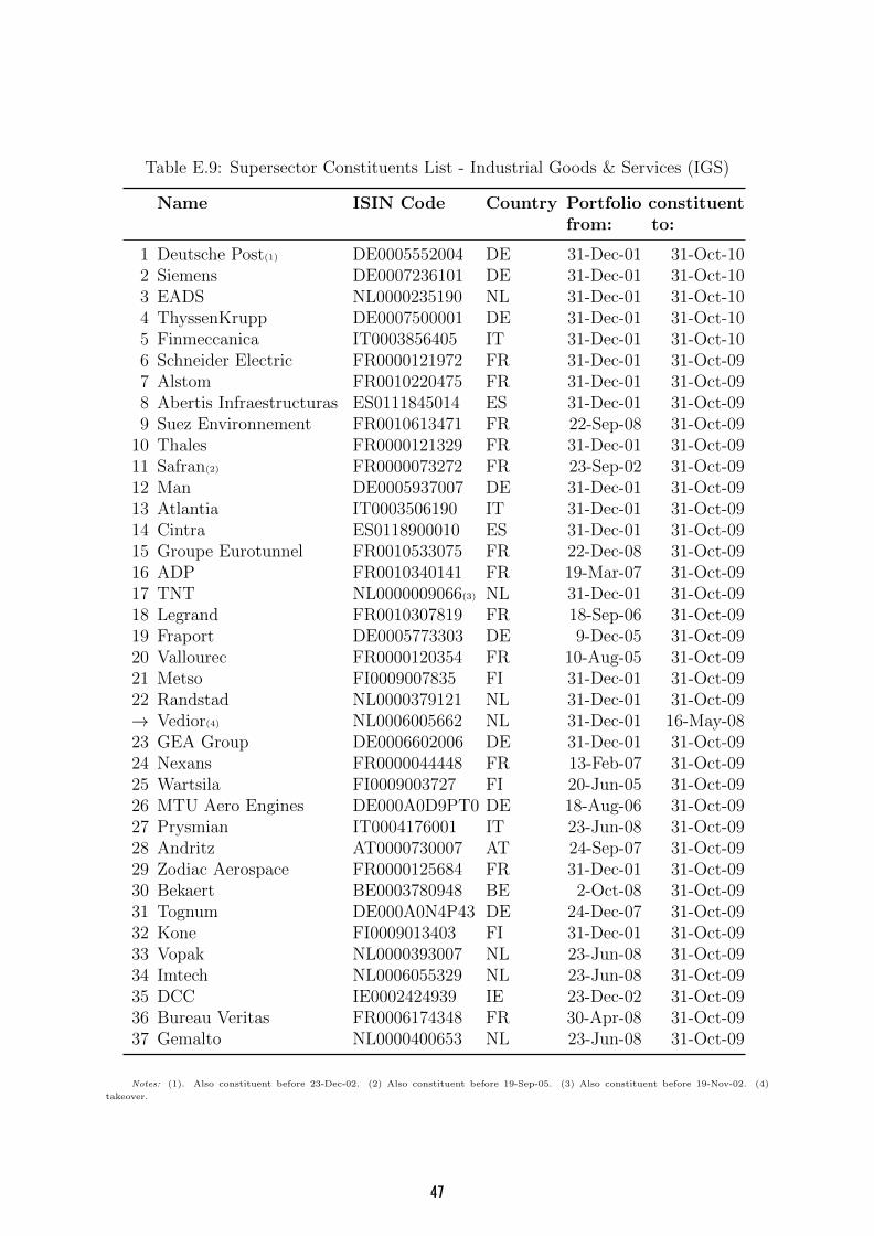
Table E.9: Supersector Constituents List - Industrial Goods & Services (IGS)
Name ISIN Code Country Portfolio constituentfrom: to:
1 Deutsche Post(1) DE0005552004 DE 31-Dec-01 31-Oct-102 Siemens DE0007236101 DE 31-Dec-01 31-Oct-103 EADS NL0000235190 NL 31-Dec-01 31-Oct-104 ThyssenKrupp DE0007500001 DE 31-Dec-01 31-Oct-105 Finmeccanica IT0003856405 IT 31-Dec-01 31-Oct-106 Schneider Electric FR0000121972 FR 31-Dec-01 31-Oct-097 Alstom FR0010220475 FR 31-Dec-01 31-Oct-098 Abertis Infraestructuras ES0111845014 ES 31-Dec-01 31-Oct-099 Suez Environnement FR0010613471 FR 22-Sep-08 31-Oct-09
10 Thales FR0000121329 FR 31-Dec-01 31-Oct-0911 Safran(2) FR0000073272 FR 23-Sep-02 31-Oct-0912 Man DE0005937007 DE 31-Dec-01 31-Oct-0913 Atlantia IT0003506190 IT 31-Dec-01 31-Oct-0914 Cintra ES0118900010 ES 31-Dec-01 31-Oct-0915 Groupe Eurotunnel FR0010533075 FR 22-Dec-08 31-Oct-0916 ADP FR0010340141 FR 19-Mar-07 31-Oct-0917 TNT NL0000009066(3) NL 31-Dec-01 31-Oct-0918 Legrand FR0010307819 FR 18-Sep-06 31-Oct-0919 Fraport DE0005773303 DE 9-Dec-05 31-Oct-0920 Vallourec FR0000120354 FR 10-Aug-05 31-Oct-0921 Metso FI0009007835 FI 31-Dec-01 31-Oct-0922 Randstad NL0000379121 NL 31-Dec-01 31-Oct-09→ Vedior(4) NL0006005662 NL 31-Dec-01 16-May-0823 GEA Group DE0006602006 DE 31-Dec-01 31-Oct-0924 Nexans FR0000044448 FR 13-Feb-07 31-Oct-0925 Wartsila FI0009003727 FI 20-Jun-05 31-Oct-0926 MTU Aero Engines DE000A0D9PT0 DE 18-Aug-06 31-Oct-0927 Prysmian IT0004176001 IT 23-Jun-08 31-Oct-0928 Andritz AT0000730007 AT 24-Sep-07 31-Oct-0929 Zodiac Aerospace FR0000125684 FR 31-Dec-01 31-Oct-0930 Bekaert BE0003780948 BE 2-Oct-08 31-Oct-0931 Tognum DE000A0N4P43 DE 24-Dec-07 31-Oct-0932 Kone FI0009013403 FI 31-Dec-01 31-Oct-0933 Vopak NL0000393007 NL 23-Jun-08 31-Oct-0934 Imtech NL0006055329 NL 23-Jun-08 31-Oct-0935 DCC IE0002424939 IE 23-Dec-02 31-Oct-0936 Bureau Veritas FR0006174348 FR 30-Apr-08 31-Oct-0937 Gemalto NL0000400653 NL 23-Jun-08 31-Oct-09
Notes: (1). Also constituent before 23-Dec-02. (2) Also constituent before 19-Sep-05. (3) Also constituent before 19-Nov-02. (4)
takeover.
47
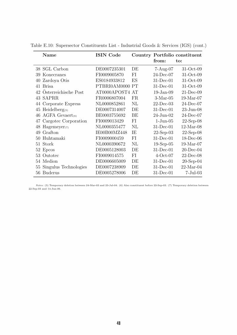
Table E.10: Supersector Constituents List - Industrial Goods & Services (IGS) (cont.)
Name ISIN Code Country Portfolio constituentfrom: to:
38 SGL Carbon DE0007235301 DE 7-Aug-07 31-Oct-0939 Konecranes FI0009005870 FI 24-Dec-07 31-Oct-0940 Zardoya Otis ES0184933812 ES 31-Dec-01 31-Oct-0941 Brisa PTBRI0AM0000 PT 31-Dec-01 31-Oct-09
42 Osterreichische Post AT0000APOST4 AT 19-Jan-09 21-Dec-0943 SAPRR FR0006807004 FR 3-Mar-05 19-Mar-0744 Corporate Express NL0000852861 NL 22-Dec-03 24-Dec-0745 Heidelberg(5) DE0007314007 DE 31-Dec-01 23-Jun-0846 AGFA Gevaert(6) BE0003755692 BE 24-Jun-02 24-Dec-0747 Cargotec Corporation FI0009013429 FI 1-Jun-05 22-Sep-0848 Hagemeyer(7) NL0000355477 NL 31-Dec-01 12-Mar-0849 Grafton IE00B00MZ448 IE 22-Sep-03 22-Sep-0850 Huhtamaki FI0009000459 FI 31-Dec-01 18-Dec-0651 Stork NL0000390672 NL 19-Sep-05 19-Mar-0752 Epcos DE0005128003 DE 31-Dec-01 20-Dec-0453 Outotec FI0009014575 FI 4-Oct-07 22-Dec-0854 Medion DE0006605009 DE 31-Dec-01 20-Sep-0455 Singulus Technologies DE0007238909 DE 31-Dec-01 22-Mar-0456 Buderus DE0005278006 DE 31-Dec-01 7-Jul-03
Notes: (5) Temporary deletion between 24-Mar-03 and 23-Jul-04. (6) Also constituent before 22-Sep-03. (7) Temporary deletion between
22-Sep-03 and 14-Jun-06.
48
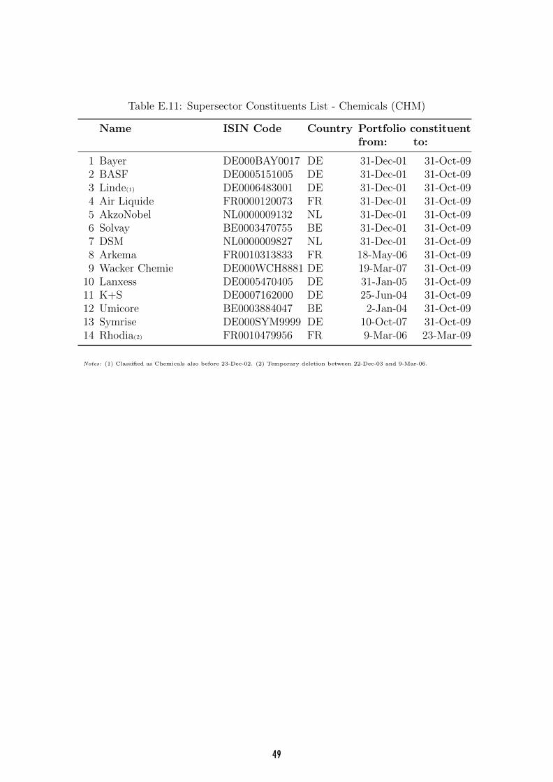
Table E.11: Supersector Constituents List - Chemicals (CHM)
Name ISIN Code Country Portfolio constituentfrom: to:
1 Bayer DE000BAY0017 DE 31-Dec-01 31-Oct-092 BASF DE0005151005 DE 31-Dec-01 31-Oct-093 Linde(1) DE0006483001 DE 31-Dec-01 31-Oct-094 Air Liquide FR0000120073 FR 31-Dec-01 31-Oct-095 AkzoNobel NL0000009132 NL 31-Dec-01 31-Oct-096 Solvay BE0003470755 BE 31-Dec-01 31-Oct-097 DSM NL0000009827 NL 31-Dec-01 31-Oct-098 Arkema FR0010313833 FR 18-May-06 31-Oct-099 Wacker Chemie DE000WCH8881 DE 19-Mar-07 31-Oct-09
10 Lanxess DE0005470405 DE 31-Jan-05 31-Oct-0911 K+S DE0007162000 DE 25-Jun-04 31-Oct-0912 Umicore BE0003884047 BE 2-Jan-04 31-Oct-0913 Symrise DE000SYM9999 DE 10-Oct-07 31-Oct-0914 Rhodia(2) FR0010479956 FR 9-Mar-06 23-Mar-09
Notes: (1) Classified as Chemicals also before 23-Dec-02. (2) Temporary deletion between 22-Dec-03 and 9-Mar-06.
49

Table E.12: Supersector Constituents List - Food & Beverage (FOB)
Name ISIN Code Country Portfolio constituentfrom: to:
1 Anheuser-Busch InBev BE0003793107 BE 31-Dec-01 31-Oct-092 Unilever NL0000009355 NL 31-Dec-01 31-Oct-093 Danone FR0000120644 FR 31-Dec-01 31-Oct-09→ Royal Numico(1) NL0000375616 NL 31-Dec-01 14-Nov-074 Pernod Ricard FR0000120693 FR 31-Dec-01 31-Oct-095 Heineken Holding(2) NL0000008977 NL 31-Dec-01 31-Oct-09→ Heineken NV NL0000009165 NL 31-Dec-01 31-Oct-096 Suedzucker(3) DE0007297004 DE 23-Sep-02 31-Oct-097 Coca-Cola HBC GRS104003009 GR 31-Dec-01 31-Oct-098 Parmalat IT0003826473 IT 20-Mar-06 31-Oct-099 Kerry Grp IE0004906560 IE 31-Dec-01 31-Oct-09
10 Ebro Puleva(4) ES0112501012 ES 23-Dec-02 31-Oct-0911 Nutreco(5) NL0000375400 NL 22-Sep-08 31-Oct-0912 CSM NL0000852549 NL 31-Dec-01 31-Oct-0913 C&C Group IE00B010DT83 IE 19-Sep-05 22-Dec-08
Notes: (1) Takeover. (2) Dual-listed. (3) Temporary deletion between 19-Mar-07 and 23-Mar-09. (4) Temporary deletion between
24-Dec-07 and 22-Dec-08. (5) Also constituent before 23-Dec-02.
50
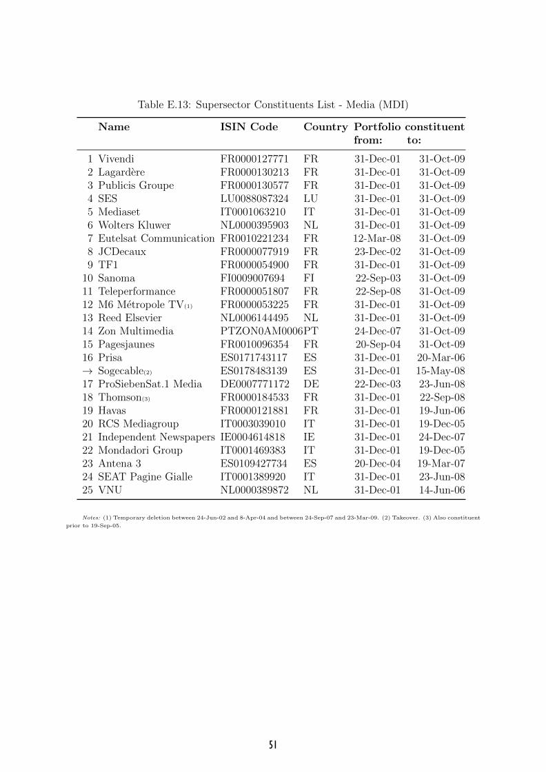
Table E.13: Supersector Constituents List - Media (MDI)
Name ISIN Code Country Portfolio constituentfrom: to:
1 Vivendi FR0000127771 FR 31-Dec-01 31-Oct-092 Lagardere FR0000130213 FR 31-Dec-01 31-Oct-093 Publicis Groupe FR0000130577 FR 31-Dec-01 31-Oct-094 SES LU0088087324 LU 31-Dec-01 31-Oct-095 Mediaset IT0001063210 IT 31-Dec-01 31-Oct-096 Wolters Kluwer NL0000395903 NL 31-Dec-01 31-Oct-097 Eutelsat Communication FR0010221234 FR 12-Mar-08 31-Oct-098 JCDecaux FR0000077919 FR 23-Dec-02 31-Oct-099 TF1 FR0000054900 FR 31-Dec-01 31-Oct-09
10 Sanoma FI0009007694 FI 22-Sep-03 31-Oct-0911 Teleperformance FR0000051807 FR 22-Sep-08 31-Oct-0912 M6 Metropole TV(1) FR0000053225 FR 31-Dec-01 31-Oct-0913 Reed Elsevier NL0006144495 NL 31-Dec-01 31-Oct-0914 Zon Multimedia PTZON0AM0006PT 24-Dec-07 31-Oct-0915 Pagesjaunes FR0010096354 FR 20-Sep-04 31-Oct-0916 Prisa ES0171743117 ES 31-Dec-01 20-Mar-06→ Sogecable(2) ES0178483139 ES 31-Dec-01 15-May-0817 ProSiebenSat.1 Media DE0007771172 DE 22-Dec-03 23-Jun-0818 Thomson(3) FR0000184533 FR 31-Dec-01 22-Sep-0819 Havas FR0000121881 FR 31-Dec-01 19-Jun-0620 RCS Mediagroup IT0003039010 IT 31-Dec-01 19-Dec-0521 Independent Newspapers IE0004614818 IE 31-Dec-01 24-Dec-0722 Mondadori Group IT0001469383 IT 31-Dec-01 19-Dec-0523 Antena 3 ES0109427734 ES 20-Dec-04 19-Mar-0724 SEAT Pagine Gialle IT0001389920 IT 31-Dec-01 23-Jun-0825 VNU NL0000389872 NL 31-Dec-01 14-Jun-06
Notes: (1) Temporary deletion between 24-Jun-02 and 8-Apr-04 and between 24-Sep-07 and 23-Mar-09. (2) Takeover. (3) Also constituent
prior to 19-Sep-05.
51
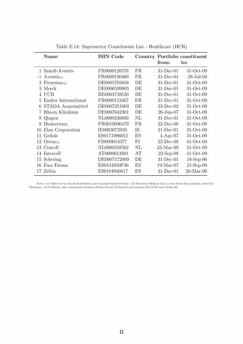
Table E.14: Supersector Constituents List - Healthcare (HCR)
Name ISIN Code Country Portfolio constituentfrom: to:
1 Sanofi-Aventis FR0000120578 FR 31-Dec-01 31-Oct-09→ Aventis(1) FR0000130460 FR 31-Dec-01 28-Jul-042 Fresenius(2) DE0005785638 DE 31-Dec-01 31-Oct-093 Merck DE0006599905 DE 31-Dec-01 31-Oct-094 UCB BE0003739530 BE 31-Dec-01 31-Oct-095 Essilor International FR0000121667 FR 31-Dec-01 31-Oct-096 STADA Arzneimittel DE0007251803 DE 23-Dec-02 31-Oct-097 Rhoen Klinikum DE0007042301 DE 26-Jun-07 31-Oct-098 Qiagen NL0000240000 NL 31-Dec-01 31-Oct-099 Biomerieux FR0010096479 FR 22-Dec-08 31-Oct-09
10 Elan Corporation IE0003072950 IE 31-Dec-01 31-Oct-0911 Grifols ES0171996012 ES 4-Apr-07 31-Oct-0912 Orion(3) FI0009014377 FI 22-Dec-08 31-Oct-0913 Crucell NL0000358562 NL 23-Mar-09 31-Oct-0914 Intercell AT0000612601 AT 22-Sep-08 31-Oct-0915 Schering DE0007172009 DE 31-Dec-01 18-Sep-0616 Faes Farma ES0134950F36 ES 19-Mar-07 21-Sep-0917 Zeltia ES0184940817 ES 31-Dec-01 20-Mar-06
Notes: (1) Takeover by Sanofi-Synthelabo and renamed Sanofi-Aventis. (2) Fresenius Medical Care is also listed but partially owned by
Fresenius. (3) B Shares, also constituent between 23-Dec-02 and 22-Sep-03 and between 28-Jul-05 and 18-Sep-06.
52