ecb economic bulletin, issue 6 / 2016 (september 2016) · ecb economic bulletin, ... euro area...
TRANSCRIPT
Economic Bulletin
Issue 6 / 2016
ECB Economic Bulletin, Issue 6 / 2016 1
Contents
Economic and monetary developments 2
Overview 2
1 External environment 5
2 Financial developments 10
3 Economic activity 13
4 Prices and costs 18
5 Money and credit 22
6 Fiscal developments 27
Boxes 30
1 Determinants of the slowdown in global trade: what is the new normal? 30
2 Financing constraints in euro area regions 34
3 Liquidity conditions and monetary policy operations in the period from 27 April to 26 July 2016 38
4 Global production patterns from a European perspective: insights from a survey of large euro area firms 43
5 What accounts for the recent decoupling between the euro area GDP deflator and the HICP excluding energy and food? 46
6 Factors behind developments in average hours worked per person employed since 2008 49
Article 53
1 The employment-GDP relationship since the crisis 53
Statistics S1

ECB Economic Bulletin, Issue 6 / 2016 – Economic and monetary developments Overview 2
Economic and monetary developments
Overview
At its monetary policy meeting on 8 September 2016, the Governing Council assessed the economic and monetary data which had become available since the July meeting and discussed the new ECB staff macroeconomic projections. The comprehensive policy measures that have been adopted continue to ensure supportive financing conditions and underpin the momentum of the euro area economic recovery. As a result, the Governing Council continues to expect real GDP to grow at a moderate but steady pace and euro area inflation to rise gradually over the coming months, in line with the path already implied in the June 2016 staff projections. Overall, while the available evidence so far suggests resilience of the euro area economy to the continuing global economic and political uncertainty, the baseline scenario remains subject to downside risks.
Economic and monetary assessment at the time of the Governing Council meeting of 8 September 2016
Moderate global growth continued in the first half of 2016. Looking ahead, global growth is expected to recover gradually. Low interest rates, improving labour markets and growing confidence support the outlook for advanced economies, although the uncertainty generated by the referendum in the United Kingdom on EU membership will weigh on demand in that country. As regards emerging market economies, economic activity in China is expected to slow, while the outlook for large commodity exporters remains subdued, despite some tentative signs of stabilisation. Risks to the outlook for global economic activity remain on the downside.
Between early June and early September euro area and global financial markets remained relatively calm, apart from the immediate period around the UK referendum. In the period leading up to the referendum on 23 June, global financial markets exhibited increasing volatility, which spiked on the day following the referendum. Since then, financial market volatility has receded and most asset classes have recovered their losses. At the same time, long-term euro area bond yields remained significantly below their pre-referendum levels, and bank equities continued to underperform the wider market index.
The economic recovery in the euro area is continuing. Euro area real GDP increased by 0.3%, quarter on quarter, in the second quarter of 2016, after 0.5% in the first quarter. Growth was supported by net exports as well as a continued positive contribution from domestic demand. Incoming data point to ongoing growth in the third quarter of 2016, at around the same rate as in the second quarter.
Looking ahead, the Governing Council expects the economic recovery to proceed at a moderate but steady pace. Domestic demand remains supported by
ECB Economic Bulletin, Issue 6 / 2016 – Economic and monetary developments Overview 3
the pass-through of the monetary policy measures to the real economy. Favourable financing conditions and improvements in the demand outlook and in corporate profitability continue to promote a recovery in investment. Sustained employment gains, which are also benefiting from past structural reforms and still relatively low oil prices provide additional support for households’ real disposable income and thus for private consumption. In addition, the fiscal stance in the euro area is expected to be mildly expansionary in 2016 and to turn broadly neutral in 2017 and 2018. However, the economic recovery in the euro area is expected to be dampened by still subdued foreign demand – partly related to the uncertainties following the UK referendum outcome – the necessary balance sheet adjustments in a number of sectors and a sluggish pace of implementation of structural reforms.
The September 2016 ECB staff macroeconomic projections for the euro area expect annual real GDP to increase by 1.7% in 2016, by 1.6% in 2017 and by 1.6% in 2018. Compared with the June 2016 Eurosystem staff macroeconomic projections, the outlook for real GDP growth has been revised downwards slightly. In the Governing Council’s assessment, the risks to the euro area growth outlook remain tilted to the downside and relate mainly to the external environment.
According to Eurostat’s flash estimate, euro area annual HICP inflation in August 2016 was 0.2%, unchanged from July. While annual energy inflation continued to rise, services and non-energy industrial goods inflation was slightly lower than in July. Looking ahead, on the basis of current oil futures prices, inflation rates are likely to remain low over the next few months before starting to pick up towards the end of 2016, in large part owing to base effects in the annual rate of change of energy prices. Supported by the ECB’s monetary policy measures and the expected economic recovery, inflation rates should increase further in 2017 and 2018.
The September 2016 ECB staff macroeconomic projections for the euro area foresee annual HICP inflation at 0.2% in 2016, 1.2% in 2017 and 1.6% in 2018. In comparison with the June 2016 Eurosystem staff macroeconomic projections, the outlook for HICP inflation is broadly unchanged.
The monetary policy measures in place since June 2014 are filtering through to borrowing conditions for firms and households and are thereby increasingly supporting credit flows across the euro area. Broad money continued to increase at a robust pace in July 2016 and loan growth continued to recover gradually. Domestic sources of money creation were again the main driver of broad money growth. Low interest rates and the effects of the ECB’s non-standard monetary policy measures continue to support money and credit dynamics. Banks have been passing on their favourable funding conditions in the form of lower lending rates and have eased credit standards, thereby supporting the recovery of loan growth. The annual flow of total external financing to non-financial corporations is estimated to have increased in the second quarter of 2016.

ECB Economic Bulletin, Issue 6 / 2016 – Economic and monetary developments Overview 4
Monetary policy decisions
The Governing Council decided to keep the key ECB interest rates unchanged and continued to expect these rates to remain at present or lower levels for an extended period of time, and well past the horizon of the Eurosystem’s net asset purchases. Regarding non-standard monetary policy measures, the Governing Council confirmed that the monthly asset purchases of €80 billion are intended to run until the end of March 2017, or beyond, if necessary, and in any case until the Governing Council sees a sustained adjustment in the path of inflation consistent with its inflation aim.
The Governing Council will remain alert and ready to act, if warranted, to achieve its price stability objective. In the light of prevailing uncertainties, the Governing Council will continue to monitor economic and financial market developments very closely. It will preserve the very substantial amount of monetary support that is embedded in the ECB staff macroeconomic projections and that is necessary to secure a return of inflation to levels below, but close to, 2% over the medium term. If warranted, the Governing Council will act by using all the instruments available within its mandate. Meanwhile, the Governing Council tasked the relevant committees to evaluate the options that ensure a smooth implementation of the Eurosystem’s asset purchase programme.

ECB Economic Bulletin, Issue 6 / 2016 – Economic and monetary developments External environment 5
1 External environment
The moderate global growth recorded towards the end of last year continued in the first half of 2016. Looking ahead, global growth is expected to recover gradually. Low interest rates, improving labour markets and resilient confidence support the outlook for advanced economies, although the uncertainty generated by the referendum in the United Kingdom on EU membership will weigh on demand in that country. As regards emerging market economies (EMEs), economic activity in China is expected to slow, while the outlook for large commodity exporters remains subdued, despite some tentative signs of stabilisation. Risks to the outlook for global economic activity remain on the downside.
Global economic activity and trade
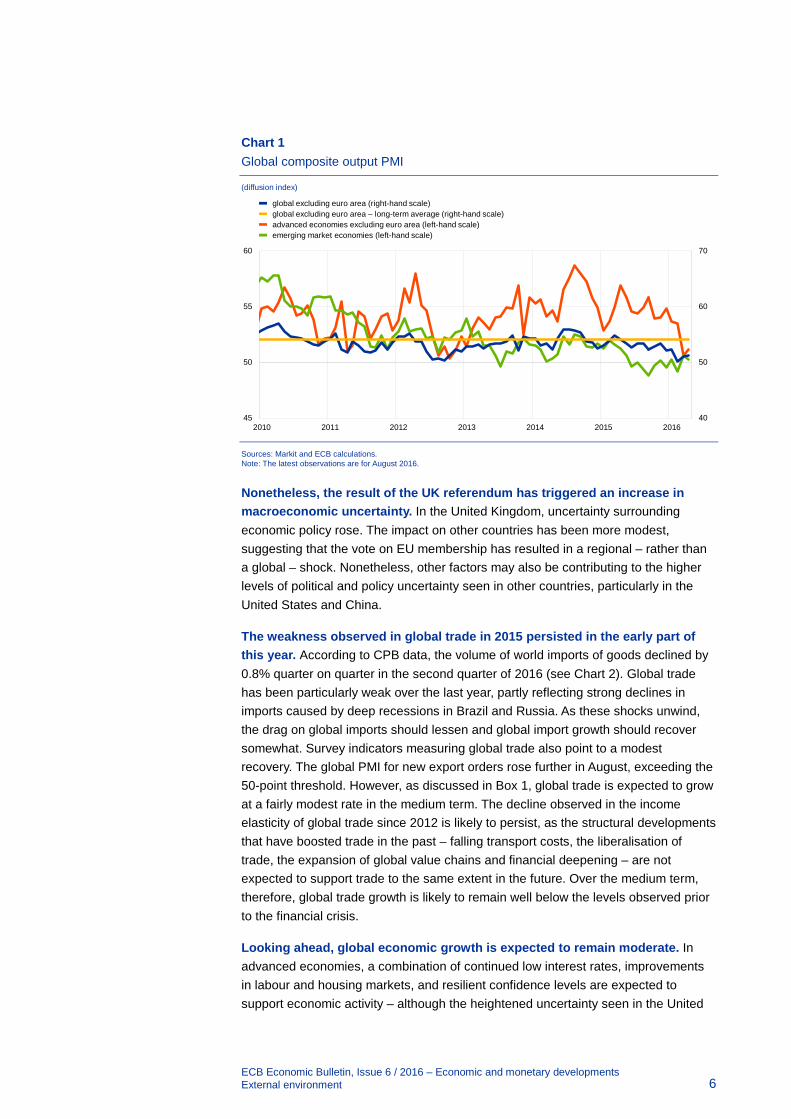
Global economic growth remains moderate. Following a soft patch in the first quarter, GDP growth in the United States strengthened only modestly in the second quarter, reflecting a large drag from inventories and a further decline in investment, driven primarily by falling capital expenditure in the energy sector. Meanwhile, economic growth in the United Kingdom was more resilient in the second quarter. In contrast, the pace of expansion in Japan slowed, after leap year effects had boosted growth in the first quarter. In China, GDP growth stabilised in the second quarter, in line with the government’s annual growth target, although economic activity relied heavily on government support through infrastructure investment and continued credit growth. While short-term indicators suggest that growth rates are beginning to bottom out in Brazil and Russia, output in those countries declined further in the second quarter. Overall, recent survey indicators suggest that global economic activity will continue to expand at a modest rate. The global composite output Purchasing Managers’ Index (PMI) remained subdued in August (see Chart 1).
The outcome of the UK referendum on EU membership surprised financial markets, but volatility has been short-lived – contained, in part, by expectations of countercyclical policy responses in major advanced economies. Following the referendum the pound declined, but the impact on most global markets outside Europe has been short-lived. Capital flows to EMEs have proved resilient, amid a broad improvement in EMEs’ financial conditions, possibly linked to search-for-yield flows out of advanced economies. The Bank of England cut interest rates and announced further quantitative easing at its meeting in August. The UK government has also announced that it now expects the pace of fiscal consolidation in the country to be slower than was previously planned. In the United States, market expectations of interest rate rises by the Federal Reserve System in 2016 fell in the immediate aftermath of the referendum, before increasing again following stronger than expected labour market data. The Bank of Japan also adopted further monetary stimulus at its meeting in July, while the Japanese government announced fiscal stimulus measures in its supplementary budget for the 2016-17 fiscal year.
ECB Economic Bulletin, Issue 6 / 2016 – Economic and monetary developments External environment 6
Chart 1 Global composite output PMI
(diffusion index)
Sources: Markit and ECB calculations. Note: The latest observations are for August 2016.
Nonetheless, the result of the UK referendum has triggered an increase in macroeconomic uncertainty. In the United Kingdom, uncertainty surrounding economic policy rose. The impact on other countries has been more modest, suggesting that the vote on EU membership has resulted in a regional – rather than a global – shock. Nonetheless, other factors may also be contributing to the higher levels of political and policy uncertainty seen in other countries, particularly in the United States and China.
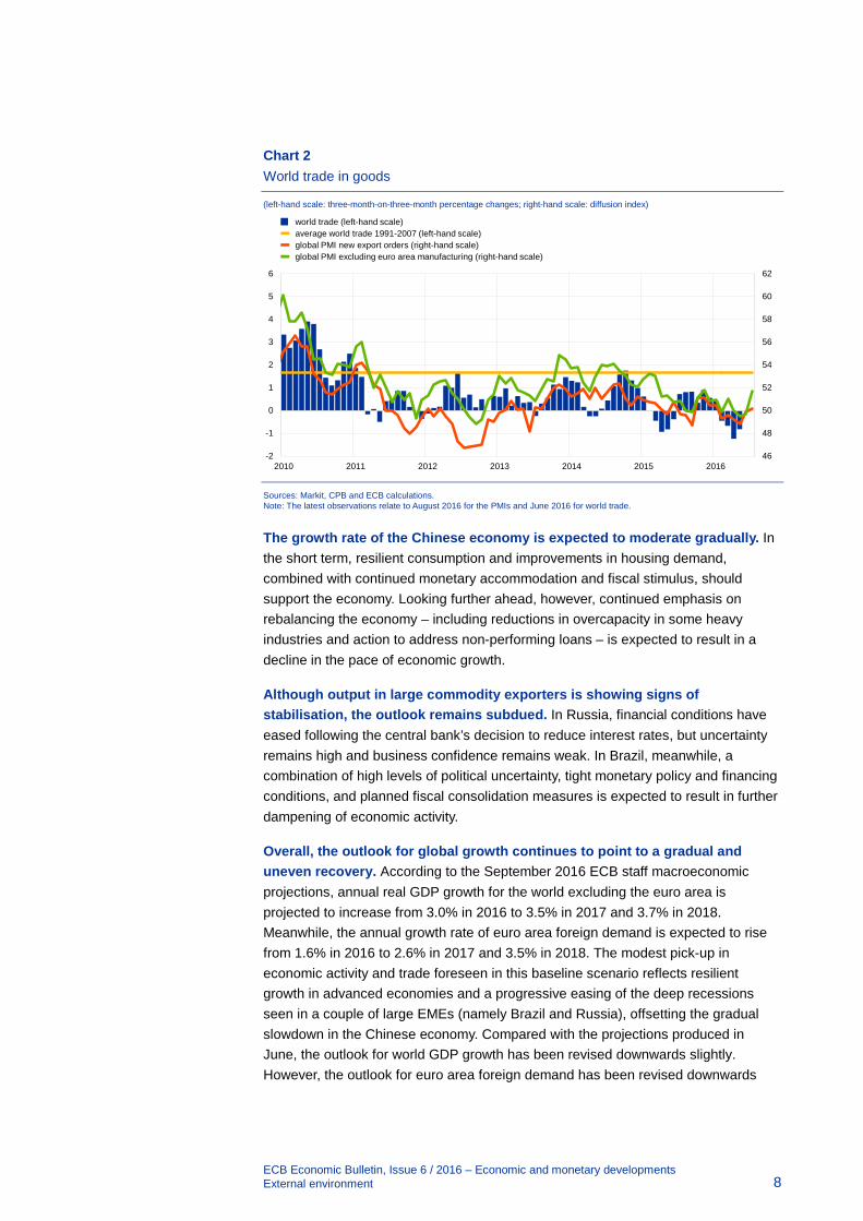
The weakness observed in global trade in 2015 persisted in the early part of this year. According to CPB data, the volume of world imports of goods declined by 0.8% quarter on quarter in the second quarter of 2016 (see Chart 2). Global trade has been particularly weak over the last year, partly reflecting strong declines in imports caused by deep recessions in Brazil and Russia. As these shocks unwind, the drag on global imports should lessen and global import growth should recover somewhat. Survey indicators measuring global trade also point to a modest recovery. The global PMI for new export orders rose further in August, exceeding the 50-point threshold. However, as discussed in Box 1, global trade is expected to grow at a fairly modest rate in the medium term. The decline observed in the income elasticity of global trade since 2012 is likely to persist, as the structural developments that have boosted trade in the past – falling transport costs, the liberalisation of trade, the expansion of global value chains and financial deepening – are not expected to support trade to the same extent in the future. Over the medium term, therefore, global trade growth is likely to remain well below the levels observed prior to the financial crisis.
Looking ahead, global economic growth is expected to remain moderate. In advanced economies, a combination of continued low interest rates, improvements in labour and housing markets, and resilient confidence levels are expected to support economic activity – although the heightened uncertainty seen in the United
40
50
60
70
45
50
55
60
2010 2011 2012 2013 2014 2015 2016
global excluding euro area (right-hand scale)global excluding euro area – long-term average (right-hand scale)advanced economies excluding euro area (left-hand scale)emerging market economies (left-hand scale)

ECB Economic Bulletin, Issue 6 / 2016 – Economic and monetary developments External environment 7
Kingdom is expected to dampen investment. Meanwhile, the gradual rebalancing of the Chinese economy is likely to weigh on growth. Capital flows to EMEs have recovered recently, but many countries are still coping with the tightening of external financing conditions associated with the expected withdrawal of monetary accommodation in the United States. The gradual easing of deep recessions in a couple of larger commodity exporters will provide some support for global growth in the years ahead, but the outlook remains subdued, as many commodity exporters face difficulties in adjusting to the low commodity price environment. Finally, increases in political uncertainty and geopolitical tensions are also weighing on demand across a number of regions.
Looking at individual countries in more detail, economic activity in the United States is expected to recover. Strong domestic fundamentals – reflected in robust job growth, modest increases in nominal wages as the economy approaches full employment, and positive household wealth effects (mostly from rising house prices) – are expected to support private consumption. Reductions in long-term interest rates and the end of the contraction in the energy sector are also expected to boost investment over the projection horizon. On the other hand, the strengthening of the US dollar and modest growth in foreign demand will weigh on exports.
The outlook for Japan remains subdued. In the short term, supply chain disruption following the earthquake in April will constrain production. Looking further ahead, however, private consumption is expected to recover amid rises in real incomes, while accommodative financial conditions should foster increases in investment. The postponement of the rise in VAT scheduled for April 2017 will support economic activity, as will the additional stimulus measures announced in the supplementary budget. In addition, monetary policy remains highly accommodative. Exports are expected to benefit from gradual improvements in foreign demand, albeit tempered by the recovery seen in the value of the yen over the last year.
The heightened uncertainty seen in the United Kingdom is expected to weigh on economic growth. The institutional and political uncertainty surrounding the negotiations to leave the European Union is expected to dampen domestic demand, particularly investment (although recent data suggest that the short-term impact of the referendum has been relatively modest thus far). Looking further ahead, monetary accommodation and a reduction in the pace of fiscal consolidation should help to support economic activity.
Real economic activity in central and eastern Europe is projected to remain relatively resilient. Private consumption is expected to be supported by increases in real disposable income and low levels of inflation. However, the uncertainty triggered by the referendum in the United Kingdom and the potential impact on the UK and euro area economies (which represent those countries’ main trading partners) are expected to weigh on output in the coming quarters.
ECB Economic Bulletin, Issue 6 / 2016 – Economic and monetary developments External environment 8
Chart 2 World trade in goods
(left-hand scale: three-month-on-three-month percentage changes; right-hand scale: diffusion index)
Sources: Markit, CPB and ECB calculations. Note: The latest observations relate to August 2016 for the PMIs and June 2016 for world trade.
The growth rate of the Chinese economy is expected to moderate gradually. In the short term, resilient consumption and improvements in housing demand, combined with continued monetary accommodation and fiscal stimulus, should support the economy. Looking further ahead, however, continued emphasis on rebalancing the economy – including reductions in overcapacity in some heavy industries and action to address non-performing loans – is expected to result in a decline in the pace of economic growth.
Although output in large commodity exporters is showing signs of stabilisation, the outlook remains subdued. In Russia, financial conditions have eased following the central bank’s decision to reduce interest rates, but uncertainty remains high and business confidence remains weak. In Brazil, meanwhile, a combination of high levels of political uncertainty, tight monetary policy and financing conditions, and planned fiscal consolidation measures is expected to result in further dampening of economic activity.
Overall, the outlook for global growth continues to point to a gradual and uneven recovery. According to the September 2016 ECB staff macroeconomic projections, annual real GDP growth for the world excluding the euro area is projected to increase from 3.0% in 2016 to 3.5% in 2017 and 3.7% in 2018. Meanwhile, the annual growth rate of euro area foreign demand is expected to rise from 1.6% in 2016 to 2.6% in 2017 and 3.5% in 2018. The modest pick-up in economic activity and trade foreseen in this baseline scenario reflects resilient growth in advanced economies and a progressive easing of the deep recessions seen in a couple of large EMEs (namely Brazil and Russia), offsetting the gradual slowdown in the Chinese economy. Compared with the projections produced in June, the outlook for world GDP growth has been revised downwards slightly. However, the outlook for euro area foreign demand has been revised downwards
46
48
50
52
54
56
58
60
62
-2
-1
0
1
2
3
4
5
6
2010 2011 2012 2013 2014 2015 2016
world trade (left-hand scale)average world trade 1991-2007 (left-hand scale)global PMI new export orders (right-hand scale)global PMI excluding euro area manufacturing (right-hand scale)

ECB Economic Bulletin, Issue 6 / 2016 – Economic and monetary developments External environment 9
more significantly, largely reflecting expectations of much weaker growth in imports from the United Kingdom.
Risks to the outlook for global economic activity remain on the downside, particularly for EMEs. A key downside risk is a stronger slowdown in EMEs (including China). A tightening of financing conditions and an increase in political uncertainty could exacerbate existing macroeconomic imbalances, denting confidence and resulting in an unexpectedly strong slowdown. Policy uncertainty surrounding the economic transition in China could lead to an increase in global financial volatility. Geopolitical risks also continue to weigh on the outlook. Moreover, the economic implications of the United Kingdom leaving the European Union could be worse than expected, increasing uncertainty and negatively affecting trade, business confidence and investment.
Global price developments
The effects of past declines in oil prices continue to weigh on global headline inflation. Average annual CPI inflation in OECD countries fell to 0.8% in July, from 0.9% in the previous month (see Chart 3). The energy component has continued to weigh on inflation, with average OECD inflation excluding food and energy standing at 1.8% in July. Looking at large EMEs, inflation fell in China, Brazil and Russia and rose modestly in India.
Oil prices have risen in recent months. Price dynamics have been shaped by developments on the supply side, with large outages in a number of OPEC countries (Libya, Nigeria and Venezuela) and one non-OPEC country (Canada) dampening excess supply conditions. More recently, however, Saudi Arabian output has reached an all-time high, the decline in the supply of US shale oil has eased, and Canadian oil production has come back online earlier than expected. At the same time, global oil demand remained stronger than expected in the first half of 2016. Over the coming months, oil prices will be supported by the rebalancing of supply/demand conditions. Meanwhile, aggregate non-oil commodity prices have remained almost unchanged in the last three months.
Looking ahead, global inflation is expected to rise gradually. In the short term, the effects of past declines in oil and other commodity prices will diminish, lessening the drag on headline inflation. Looking further
ahead, the upward-sloping oil futures curve points to increases in oil prices over the projection horizon. At the same time, the abundance of spare capacity at global level is expected to weigh on underlying inflation over the medium term.
Chart 3 Consumer price inflation
(year-on-year percentage changes)
Sources: National sources and OECD. Note: The latest observations relate to July 2016 for individual countries, except Russia, August 2016 and July 2016 for the OECD aggregate.
0
2
4
6
8
10
12
14
16
18
2010 2011 2012 2013 2014 2015 2016
ChinaBrazilRussiaIndiaOECD aggregate

ECB Economic Bulletin, Issue 6 / 2016 – Economic and monetary developments Financial developments 10
2 Financial developments
Apart from the immediate period around the UK referendum, euro area and global financial markets remained relatively calm between early June and early September. In the period leading up to the UK referendum on 23 June, global financial markets exhibited increasing volatility, which spiked on the day following the referendum. Since then, financial market volatility has receded and most asset classes have recovered their losses. The main exceptions to this normalisation are long-term euro area bond yields, which remain significantly below their pre-referendum levels, as well as bank equities, which continue to underperform the wider market index.
The relatively tranquil developments in financial markets seen during the second quarter of 2016 have continued. Against the backdrop of timid improvements in the global economic outlook, mainly fuelled by developments in the US economy, euro area and global financial markets weathered well the immediate impact of the UK vote to leave the EU. There was an initial reaction in the euro area: the euro depreciated markedly against the US dollar, the EONIA forward curve flattened, sovereign and corporate bond spreads widened, implied volatilities went up, and equities – notably bank equities – declined. Since then, financial market volatility has receded, sovereign spreads have tightened, and most other asset classes have recovered their losses. While it cannot be ruled out that financial markets may react again when the modalities of the UK’s relationship with the EU are known with more certainty, the immediate adverse impacts of this event on financial markets were short-lived.
The euro overnight index average (EONIA) remained stable during the review period (from 2 June to 7 September), while the EONIA forward curve flattened, mainly in the wake of the UK referendum (see Chart 4). Market-based expectations of future EONIA rates have been gradually declining. On 2 June it was expected that the EONIA rate would move into positive territory in 2021, but at the end of the review period this had been pushed back by at least one year. The expected trajectory of the EONIA rate has also undergone revision. Chart 4 illustrates that the EONIA forward rate curve moved backwards in time and also further downwards during the period under review. These developments indicate that markets may be expecting additional policy accommodation. The EONIA rate ranged between -32 and -35 basis points, except at the end of the second quarter of 2016, when it temporarily rose to -29 basis points. Excess liquidity
increased by around €192 billion, to around €1,040 billion, in the context of Eurosystem purchases under the expanded asset purchase programme. Box 3 presents more detailed information on euro area liquidity conditions and monetary policy operations.
Chart 4 EONIA forward rates
(percentages per annum)
Sources: Thomson Reuters and ECB calculations.
-0.75
-0.50
-0.25
0.00
0.25
0.50
0.75
1.00
1.25
1.50
2016 2017 2018 2019 2020 2021 2022 2023 2024 2025
7 September 20162 June 2016

ECB Economic Bulletin, Issue 6 / 2016 – Economic and monetary developments Financial developments 11
While euro area long-term yields generally moved closely in line with their global counterparts prior to the UK referendum, a moderate widening of the existing wedge between rates in the United States and the euro area was seen in the post-referendum period, and UK long-term yields also declined markedly (see Chart 5). These developments are likely attributable to market perceptions of different economic situations and monetary policies across these economic areas. Amid low bond market volatility, the GDP-weighted average of ten-year euro area government bond yields hovered at low levels from end-June to 7 September. Country differences remained, with German ten-year yields being negative and further – albeit marginal – decreases in Portuguese, Spanish and Italian ten-year yields. These developments should also be seen in the light of the ECB’s ongoing public sector purchase programme.
Chart 6 Euro area corporate bond yields
(percentages per annum)
Source: Thomson Reuters. Note: The last observation is for 7 September 2016.
Yields on bonds issued by non-financial corporations (NFCs) continue to be positively affected by the corporate sector purchase programme (CSPP). After a downward trend in NFC bond yields, a plateau at around 0.45% seems to have been reached towards the end of July. The current levels are more than 80 basis points below those observed at the beginning of the year and can to a large extent be attributed to the CSPP (see also Box 2 in the August 2016 issue of the Economic Bulletin). Yields on bank bonds followed a similar pattern, although their decline has been less pronounced.
Global equity markets reacted strongly to the outcome of the UK referendum, with euro area banks being most affected. Euro area non-bank and US bank and non-bank equity indices have recovered the initial price drops that were seen after the UK referendum. For these equities, the prices observed at the end of the review period surpassed those seen in early June. Although euro area bank equities have
0.4
0.6
0.8
1.0
1.2
1.4
1.6
01/16 02/16 03/16 04/16 05/16 06/16 07/16 08/16 09/16
financialsnon-financials
Chart 5 Ten-year sovereign bond yields in the euro area, the United States and the United Kingdom
(percentages per annum)
Source: Thomson Reuters. Notes: The item “euro area” denotes the GDP-weighted average of ten-year sovereign bond yields. The item “United States” denotes the ten-year Treasury yield. The item “United Kingdom” denotes the ten-year gilt yield. The last observation is for 7 September 2016.
0.0
0.5
1.0
1.5
2.0
2.5
3.0
01/15 03/15 05/15 07/15 09/15 11/15 01/16 03/16 05/16 07/16 09/16
euro areaUnited StatesUnited Kingdom

ECB Economic Bulletin, Issue 6 / 2016 – Economic and monetary developments Financial developments 12
displayed a strong increase since the low point that was reached on 6 July, they continue to significantly underperform the wider market, especially from a longer-term perspective.
Chart 8 Changes in the exchange rate of the euro against selected currencies
(percentages)
Source: ECB. Notes: EER-38 is the nominal effective exchange rate of the euro against the currencies of 38 of the euro area’s most important trading partners.
In foreign exchange markets, the euro has remained virtually unchanged in effective terms. This largely reflected an appreciation of the euro by 9.3% against the pound sterling, amid heightened uncertainty after the outcome of the UK referendum, which was offset by a weakening of the euro against most other major currencies, with the exception of the US dollar. In particular, increased volatility and a decline in risk appetite supported the Japanese yen, leading to a depreciation of the euro against the Japanese currency of around 5.9%. The euro also depreciated slightly against the Swiss franc and, to a larger extent, against the currencies of most emerging market economies and commodity-exporting countries (see Chart 8).
-15 -10 -5 0 5 10 15
Croatian kunaIndian rupeeBrazilian realTaiwan dollarRomanian leuDanish krone
Hungarian forintIndonesian rupiahSouth Korean won
Turkish liraRussian roubleSwedish kronaCzech koruna
Polish zlotyJapanese yen
Swiss francPound sterling
US dollarChinese renminbi
EER-38
since 1 September 2015since 2 June 2016
Chart 7 Euro area and US equity price indices
(1 January 2016 = 100)
Sources: Thomson Reuters and ECB calculations. Note: The last observation is for 7 September 2016.
60
70
80
90
100
110
01/16 02/16 03/16 04/16 05/16 06/16 07/16 08/16 09/16
euro area bankseuro area non-banksUnited States banksUnited States non-banks

ECB Economic Bulletin, Issue 6 / 2016 – Economic and monetary developments Economic activity 13
3 Economic activity
Euro area real GDP growth normalised in the second quarter, after a strong outcome in the first quarter. Growth was supported by net exports as well as small continued positive contributions from domestic demand. The latest survey indicators have shown resilience and point to ongoing moderate growth in the third quarter. Looking ahead, the euro area economic recovery is expected to proceed at a moderate but steady pace. Tailwinds to domestic demand continue to come from the pass-through of the ECB’s monetary policy measures to the real economy. Favourable financing conditions, reduced leverage ratios and improvements in corporate profitability continue to promote investment. Sustained employment gains, which are also benefiting from past structural reforms, and still relatively low oil prices should provide additional support for households’ real disposable income and private consumption. In addition, the fiscal stance in the euro area is expected to be mildly expansionary in 2016 and to turn broadly neutral in 2017 and 2018. The weak external environment, the slow pace of structural reform, as well as balance sheet adjustment in a number of sectors, continue to weigh on the euro area growth outlook. Moreover, the outcome of the EU referendum in the United Kingdom is expected to further dampen euro area external demand. The September 2016 ECB staff macroeconomic projections foresee euro area real GDP growing by 1.7% in 2016 and by 1.6% in 2017 and 2018.
The euro area economic expansion is continuing, with real GDP growth normalising in the second quarter of 2016, following strong increases in the first quarter. Real GDP growth slowed to 0.3%, quarter on quarter, in the second quarter of 2016, down from 0.5% in the first quarter. On the production side, value added expanded by 0.3%, quarter on quarter, and was driven by industry (excluding construction) and services, whereas value added in construction fell. At the country level, real GDP came out stronger than the previous quarter in Germany, Spain and the Netherlands, while France and Italy displayed zero growth. Overall, activity was supported by a positive contribution from net exports and by a continued positive contribution from domestic demand, albeit smaller than in the previous quarter.
Private consumption, which has been the main driver of the economic recovery in recent years, rose only modestly in the second quarter. This slowdown compared with the first quarter may reflect
some normalisation following the strong growth in consumption in the first quarter. Nevertheless, consumption is expected to continue to be one of the main drivers of the ongoing recovery, in particular as labour markets continue to recover and consumer confidence remains elevated.
Chart 9 Euro area real GDP and its components
(quarter-on-quarter percentage changes and quarter-on-quarter percentage point contributions)
Source: Eurostat. Note: The latest observation is for the second quarter of 2016.
-1.00
-0.75
-0.50
-0.25
0.00
0.25
0.50
0.75
1.00
2010 2011 2012 2013 2014 2015 2016
GDP at market priceprivate consumptiongovernment consumptiongross fixed capital formationnet exportschanges in inventories
ECB Economic Bulletin, Issue 6 / 2016 – Economic and monetary developments Economic activity 14
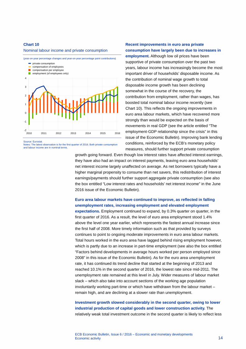
Recent improvements in euro area private consumption have largely been due to increases in employment. Although low oil prices have been supportive of private consumption over the past two years, labour income has increasingly become the most important driver of households’ disposable income. As the contribution of nominal wage growth to total disposable income growth has been declining somewhat in the course of the recovery, the contribution from employment, rather than wages, has boosted total nominal labour income recently (see Chart 10). This reflects the ongoing improvements in euro area labour markets, which have recovered more strongly than would be expected on the basis of movements in real GDP (see the article entitled “The employment-GDP relationship since the crisis” in this issue of the Economic Bulletin). Improving bank lending conditions, reinforced by the ECB’s monetary policy measures, should further support private consumption
growth going forward. Even though low interest rates have affected interest earnings, they have also had an impact on interest payments, leaving euro area households’ net interest income largely unaffected on average. As net borrowers typically have a higher marginal propensity to consume than net savers, this redistribution of interest earnings/payments should further support aggregate private consumption (see also the box entitled “Low interest rates and households’ net interest income” in the June 2016 issue of the Economic Bulletin).
Euro area labour markets have continued to improve, as reflected in falling unemployment rates, increasing employment and elevated employment expectations. Employment continued to expand, by 0.3% quarter on quarter, in the first quarter of 2016. As a result, the level of euro area employment stood 1.4% above the level one year earlier, which represents the fastest annual increase since the first half of 2008. More timely information such as that provided by surveys continues to point to ongoing moderate improvements in euro area labour markets. Total hours worked in the euro area have lagged behind rising employment however, which is partly due to an increase in part-time employment (see also the box entitled “Factors behind developments in average hours worked per person employed since 2008” in this issue of the Economic Bulletin). As for the euro area unemployment rate, it has continued its trend decline that started at the beginning of 2013 and reached 10.1% in the second quarter of 2016, the lowest rate since mid-2011. The unemployment rate remained at this level in July. Wider measures of labour market slack – which also take into account sections of the working age population involuntarily working part-time or which have withdrawn from the labour market – remain high, and are declining at a slower rate than unemployment.
Investment growth slowed considerably in the second quarter, owing to lower industrial production of capital goods and lower construction activity. The relatively weak total investment outcome in the second quarter is likely to reflect less
Chart 10 Nominal labour income and private consumption
(year-on-year percentage changes and year-on-year percentage point contributions)
Source: Eurostat. Notes: The latest observation is for the first quarter of 2016. Both private consumption and labour income are in nominal terms.
-2
-1
0
1
2
3
4
2010 2011 2012 2013 2014 2015 2016
private consumptioncompensation of employeescompensation per employeeemployment (of employees only)
ECB Economic Bulletin, Issue 6 / 2016 – Economic and monetary developments Economic activity 15
housing investment, following the favourable weather conditions in the previous quarter, which led to relatively higher construction output in that quarter. Weak capital goods production, in part related to the subdued external environment, was also an important factor – together with lower capacity utilisation – holding back business investment.
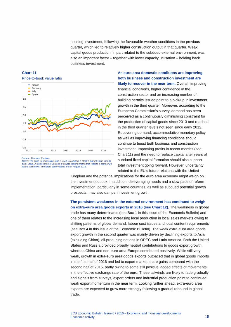
As euro area domestic conditions are improving, both business and construction investment are likely to recover in the near term. Overall, improving financial conditions, higher confidence in the construction sector and an increasing number of building permits issued point to a pick-up in investment growth in the third quarter. Moreover, according to the European Commission’s survey, demand has been perceived as a continuously diminishing constraint for the production of capital goods since 2013 and reached in the third quarter levels not seen since early 2012. Recovering demand, accommodative monetary policy as well as improving financing conditions should continue to boost both business and construction investment. Improving profits in recent months (see Chart 11) and the need to replace capital after years of subdued fixed capital formation should also support total investment going forward. However, uncertainty related to the EU’s future relations with the United
Kingdom and the potential implications for the euro area economy might weigh on the investment outlook. In addition, deleveraging needs and a slow pace of reform implementation, particularly in some countries, as well as subdued potential growth prospects, may also dampen investment growth.
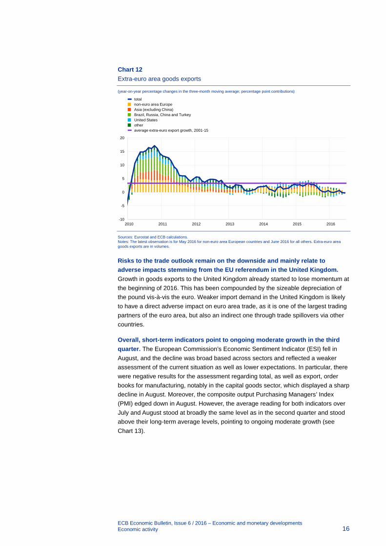
The persistent weakness in the external environment has continued to weigh on extra-euro area goods exports in 2016 (see Chart 12). The weakness in global trade has many determinants (see Box 1 in this issue of the Economic Bulletin) and one of them relates to the increasing local production in local sales markets owing to shifting patterns of global demand, labour cost issues and local content requirements (see Box 4 in this issue of the Economic Bulletin). The weak extra-euro area goods export growth in the second quarter was mainly driven by declining exports to Asia (excluding China), oil-producing nations in OPEC and Latin America. Both the United States and Russia provided broadly neutral contributions to goods export growth, whereas China and non-euro area Europe contributed positively. While still very weak, growth in extra-euro area goods exports outpaced that in global goods imports in the first half of 2016 and led to export market share gains compared with the second half of 2015, partly owing to some still positive lagged effects of movements in the effective exchange rate of the euro. These tailwinds are likely to fade gradually and signals from surveys, export orders and industrial production point to continued weak export momentum in the near term. Looking further ahead, extra-euro area exports are expected to grow more strongly following a gradual rebound in global trade.
Chart 11 Price-to-book value ratio
Source: Thomson Reuters. Notes: The price-to-book value ratio is used to compare a stock’s market value with its book value. A stock’s market value is a forward-looking metric that reflects a company’s future cash flows. The latest observations are for August 2016.
0.0
0.5
1.0
1.5
2.0
2.5
3.0
2010 2011 2012 2013 2014 2015 2016
FranceGermanyItalySpain
ECB Economic Bulletin, Issue 6 / 2016 – Economic and monetary developments Economic activity 16
Chart 12 Extra-euro area goods exports
(year-on-year percentage changes in the three-month moving average; percentage point contributions)
Sources: Eurostat and ECB calculations. Notes: The latest observation is for May 2016 for non-euro area European countries and June 2016 for all others. Extra-euro area goods exports are in volumes.
Risks to the trade outlook remain on the downside and mainly relate to adverse impacts stemming from the EU referendum in the United Kingdom. Growth in goods exports to the United Kingdom already started to lose momentum at the beginning of 2016. This has been compounded by the sizeable depreciation of the pound vis-à-vis the euro. Weaker import demand in the United Kingdom is likely to have a direct adverse impact on euro area trade, as it is one of the largest trading partners of the euro area, but also an indirect one through trade spillovers via other countries.
Overall, short-term indicators point to ongoing moderate growth in the third quarter. The European Commission’s Economic Sentiment Indicator (ESI) fell in August, and the decline was broad based across sectors and reflected a weaker assessment of the current situation as well as lower expectations. In particular, there were negative results for the assessment regarding total, as well as export, order books for manufacturing, notably in the capital goods sector, which displayed a sharp decline in August. Moreover, the composite output Purchasing Managers’ Index (PMI) edged down in August. However, the average reading for both indicators over July and August stood at broadly the same level as in the second quarter and stood above their long-term average levels, pointing to ongoing moderate growth (see Chart 13).
-10
-5
0
5
10
15
20
2010 2011 2012 2013 2014 2015 2016
totalnon-euro area EuropeAsia (excluding China)Brazil, Russia, China and TurkeyUnited Statesotheraverage extra-euro export growth, 2001-15

ECB Economic Bulletin, Issue 6 / 2016 – Economic and monetary developments Economic activity 17
Chart 14 Euro area real GDP (including projections)
(quarter-on-quarter percentage changes)
Sources: Eurostat and the article entitled “September 2016 ECB staff macroeconomic projections for the euro area”, published on the ECB’s website on 8 September 2016. Notes: The ranges shown around the central projections are based on the differences between actual outcomes and previous projections carried out over a number of years. The width of the ranges is twice the average absolute value of these differences. The method used for calculating the ranges, involving a correction for exceptional events, is documented in “New procedure for constructing Eurosystem and ECB staff projection ranges”, ECB, December 2009, available on the ECB’s website.
Looking ahead, the economic expansion in the euro area is expected to proceed at a moderate but steady pace. Domestic demand is expected to remain resilient, supported by the ECB’s accommodative monetary policy stance and supportive fiscal policy in 2016. Investment should be promoted by further improvements in corporate profitability as well as the need to modernise the capital stock after years of subdued investment. Consumer spending is expected to be sustained by ongoing employment gains, improved bank lending conditions and the still relatively low price of oil. However, the economic recovery in the euro area is expected to be dampened by still subdued foreign demand, partly related to the uncertainties following the UK referendum outcome, the necessary balance sheet adjustments in a number of sectors and a sluggish pace of implementation of structural reforms.
The September 2016 ECB staff macroeconomic projections for the euro area foresee annual real GDP increasing by 1.7% in 2016 and 1.6% in 2017 and 2018 (see Chart 14). Compared with the June 2016 Eurosystem staff macroeconomic projections, the outlook for real GDP growth has been slightly revised downwards. The risks to the euro area growth outlook remain tilted to the downside and relate mainly to the external environment.
-1.0
-0.5
0.0
0.5
1.0
1.5
2010 2011 2012 2013 2014 2015 2016 2017 2018
GDPprojection range
Chart 13 Euro area real GDP, the composite output PMI and the ESI
(quarterly growth rates and normalised percentage balances; diffusion indices)
Sources: Markit, European Commission and Eurostat. Notes: The latest observations are for the second quarter of 2016 for GDP and August 2016 for the ESI and the PMI.
-1.5
-1.0
-0.5
0.0
0.5
1.0
1.5
2.0
2010 2011 2012 2013 2014 2015 2016
real GDP (quarter-on-quarter rates)ESI composite output PMI
ECB Economic Bulletin, Issue 6 / 2016 – Economic and monetary developments Prices and costs 18
4 Prices and costs
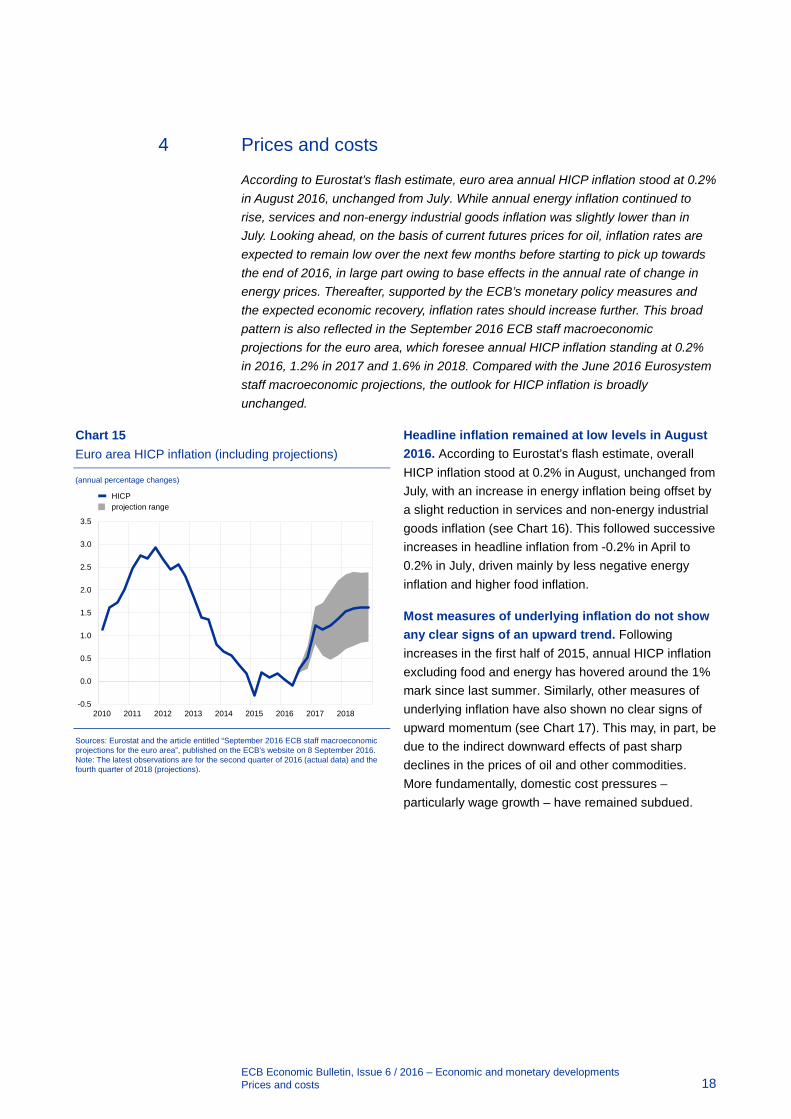
According to Eurostat’s flash estimate, euro area annual HICP inflation stood at 0.2% in August 2016, unchanged from July. While annual energy inflation continued to rise, services and non-energy industrial goods inflation was slightly lower than in July. Looking ahead, on the basis of current futures prices for oil, inflation rates are expected to remain low over the next few months before starting to pick up towards the end of 2016, in large part owing to base effects in the annual rate of change in energy prices. Thereafter, supported by the ECB’s monetary policy measures and the expected economic recovery, inflation rates should increase further. This broad pattern is also reflected in the September 2016 ECB staff macroeconomic projections for the euro area, which foresee annual HICP inflation standing at 0.2% in 2016, 1.2% in 2017 and 1.6% in 2018. Compared with the June 2016 Eurosystem staff macroeconomic projections, the outlook for HICP inflation is broadly unchanged.
Headline inflation remained at low levels in August 2016. According to Eurostat’s flash estimate, overall HICP inflation stood at 0.2% in August, unchanged from July, with an increase in energy inflation being offset by a slight reduction in services and non-energy industrial goods inflation (see Chart 16). This followed successive increases in headline inflation from -0.2% in April to 0.2% in July, driven mainly by less negative energy inflation and higher food inflation.
Most measures of underlying inflation do not show any clear signs of an upward trend. Following increases in the first half of 2015, annual HICP inflation excluding food and energy has hovered around the 1% mark since last summer. Similarly, other measures of underlying inflation have also shown no clear signs of upward momentum (see Chart 17). This may, in part, be due to the indirect downward effects of past sharp declines in the prices of oil and other commodities. More fundamentally, domestic cost pressures – particularly wage growth – have remained subdued.
Chart 15 Euro area HICP inflation (including projections)
(annual percentage changes)
Sources: Eurostat and the article entitled “September 2016 ECB staff macroeconomic projections for the euro area”, published on the ECB’s website on 8 September 2016. Note: The latest observations are for the second quarter of 2016 (actual data) and the fourth quarter of 2018 (projections).
-0.5
0.0
0.5
1.0
1.5
2.0
2.5
3.0
3.5
2010 2011 2012 2013 2014 2015 2016 2017 2018
HICPprojection range

ECB Economic Bulletin, Issue 6 / 2016 – Economic and monetary developments Prices and costs 19
Chart 16 Contributions of components to euro area headline HICP inflation
(annual percentage changes; percentage point contributions)
Sources: Eurostat and ECB calculations. Note: The latest observations are for August 2016 (flash estimates).
Pipeline pressures have remained weak. The annual growth rate of import prices for non-food consumer goods was -1.3% in July, down from -0.7% in June, and close to the recent low of -1.4% recorded in April (see Chart 18). This pattern reflects mainly the impact of developments in the euro’s nominal effective exchange rate (NEER). Further along the pricing chain, producer prices for domestic sales of non-food consumer goods remained stable, with their annual growth rate standing at 0.0% in July, unchanged from June. While the improvements seen in economic conditions are likely to have exerted upward pressure on producer prices, this may have been offset by low commodity-related input prices.
Developments in the GDP deflator suggest that domestic price pressures have strengthened since mid-2014. This reflects increases in profit margins, as labour costs have remained subdued. Those increases in profit margins likely reflect changes in terms of trade associated with falling oil prices (see the box entitled “What accounts for the recent decoupling between the euro area GDP deflator and the HICP excluding energy and food?” in this issue of the Economic Bulletin). Wage growth has remained moderate, owing to a range of factors including the still significant degree of labour market slack and weak productivity growth.1 The annual growth rate of negotiated wages stood at 1.4% in the second quarter of 2016, unchanged from the first quarter.
1 See the box entitled “Recent wage trends in the euro area”, Economic Bulletin, Issue 3, ECB, 2016.
-1.5
-1.0
-0.5
0.0
0.5
1.0
1.5
2.0
2.5
3.0
3.5
2010 2011 2012 2013 2014 2015 2016
HICPfoodenergynon-energy industrial goodsservices

ECB Economic Bulletin, Issue 6 / 2016 – Economic and monetary developments Prices and costs 20
Chart 18 Producer prices and import prices
(annual percentage changes)
Sources: Eurostat and ECB calculations. Notes: Monthly data. The latest observations are for July 2016 for import prices and producer prices and to August 2016 for the NEER-38. The NEER-38 is inverted.
Market-based measures of long-term inflation expectations have declined further and remain substantially lower than survey-based measures of expectations. Market-based measures of long-term inflation expectations declined between early June and early September. The five-year forward inflation rate five years ahead declined from 1.48% in early June to 1.29% in early September (see Chart 19). Particularly sharp declines were observed around the time of the UK referendum (partly owing to technical factors relating to safe-haven flows into nominal assets). Financial market conditions subsequently normalised, but the five-year forward inflation rate five years ahead recovered only slightly from the low of 1.25% recorded on 10 July. At the same time, markets are continuing to price in only a limited risk of deflation. In contrast, survey-based measures of long-term inflation expectations for the euro area (such as the ECB’s Survey of Professional Forecasters) have remained broadly unchanged.
Looking ahead, HICP inflation in the euro area is projected to pick up towards the end of 2016, before increasing further in 2017 and 2018. On the basis of the information available in mid-August, the September 2016 ECB staff macroeconomic projections for the euro area foresee HICP inflation standing at 0.2% in 2016, before rising to 1.2% in 2017 and 1.6% in 2018 (see Chart 15).2 Compared with the June 2016 Eurosystem staff macroeconomic projections, the outlook for HICP inflation is broadly unchanged.
2 See the article entitled “September 2016 ECB staff macroeconomic projections for the euro area”,
published on the ECB’s website on 8 September 2016.
-4
-2
0
2
4
6
-10
-5
0
5
10
15
2010 2011 2012 2013 2014 2015 2016
producer price index (right-hand scale)NEER-38 (inverted; left-hand scale)extra-euro area import prices (right-hand scale)
Chart 17 Measures of underlying inflation
(annual percentage changes)
Sources: Eurostat and ECB calculations. Notes: The range of underlying inflation measures includes the following: HICP excluding energy; HICP excluding unprocessed food and energy; HICP excluding food and energy; HICP excluding food, energy, travel-related items and clothing; the 10% trimmed mean; the 30% trimmed mean; the median of the HICP; and a measure based on a dynamic factor model. The latest observations are for August 2016 for HICP inflation excluding food and energy (flash estimate) and July 2016 for all other measures.
0.0
0.5
1.0
1.5
2.0
2.5
3.0
2010 2011 2012 2013 2014 2015 2016
HICP excluding food and energyHICP excluding food, energy, travel-related items and clothingrange of underlying inflation measures

ECB Economic Bulletin, Issue 6 / 2016 – Economic and monetary developments Prices and costs 21
Underlying inflation is expected to gradually rise over the projection horizon as upward pressures stemming from fading economic slack slowly build up. Improvements in labour market conditions, as reflected in a marked decline in the unemployment rate, are expected to bolster a gradual pick-up in wage growth and underlying inflation over the projection horizon. Amid the ongoing economic recovery, some further upward pressure on underlying inflation is also expected to materialise via improvements in corporations’ price-setting power and a related cyclical pick-up in profit margins. The fading of the dampening indirect effects of energy and non-energy commodity price developments should also contribute to the expected increase in underlying inflation. Upward effects can also be expected as a result of rising global price pressures more generally, but the gradual fading of upward pressures stemming from past declines in the value of the euro is expected to weigh on the pick-up in underlying inflation in the coming years. Overall, a
gradual pick-up in underlying inflation should support increases in headline inflation in the course of 2017 and 2018.
Chart 19 Market-based measures of inflation expectations
(annual percentage changes)
Sources: Thomson Reuters and ECB calculations. Note: The latest observations are for 7 September 2016.
0.0
0.5
1.0
1.5
2.0
2.5
3.0
01/14 05/14 09/14 01/15 05/15 09/15 01/16 05/16 09/16
one-year rate one year ahead one-year rate two years aheadone-year rate four years aheadone-year rate nine years aheadfive-year rate five years ahead

ECB Economic Bulletin, Issue 6 / 2016 – Economic and monetary developments Money and credit 22
5 Money and credit
Money growth remained robust in the second quarter of 2016 and in July. In addition, loan growth continued to recover gradually. Domestic sources of money creation were again the main driver of broad money growth. Low interest rates and the effects of the ECB’s non-standard monetary policy measures continue to support money and credit dynamics. Banks have been passing on their favourable funding conditions to lower lending rates and have eased credit standards, thereby supporting the recovery of loan growth. The annual flow of total external financing to non-financial corporations (NFCs) is estimated to have increased in the second quarter of 2016.
Broad money continued to grow at a robust pace. The annual growth rate of M3 moderated slightly to 4.8% in July 2016, having hovered around 5.0% since April 2015 (see Chart 20). The growth in M3 continued to be supported by its most liquid components, against the background of the low opportunity cost of holding these deposits in an environment of very low interest rates and a flat yield curve. In addition to the low opportunity cost of holding liquidity, robust M3 growth reflects the impact of the non-standard monetary policy measures, in particular inflows relating to the sale of securities by the money-holding sector in the context of the Eurosystem’s asset purchase programme (APP) and the targeted longer-term refinancing operations (TLTROs). The growth rate of M1 has declined during recent months, from its peak in July 2015, but still remains at a high level.
Chart 21 M3 and its components
(annual percentage changes; contributions in percentage points; adjusted for seasonal and calendar effects)
Source: ECB. Note: The latest observation is for July 2016.
Overnight deposits, which account for around half of the amount outstanding of M3 and for the bulk of M1, continued to be the main driver of M3 growth (see Chart 21). In particular, overnight deposits of the non-financial private sector
-8
-6
-4
-2
0
2
4
6
8
10
12
2008 2009 2010 2011 2012 2013 2014 2015 2016
M3 currency in circulationovernight depositsmarketable instrumentsother short-term deposits
Chart 20 M3, M1 and loans to the private sector
(annual percentage changes; adjusted for seasonal and calendar effects)
Source: ECB. Notes: Loans are adjusted for loan sales, securitisation and notional cash pooling. The latest observation is for July 2016.
-4
-2
0
2
4
6
8
10
12
14
2008 2009 2010 2011 2012 2013 2014 2015 2016
M3M1loans to the private sector

ECB Economic Bulletin, Issue 6 / 2016 – Economic and monetary developments Money and credit 23
continued to grow strongly, whereas those of non-bank financial institutions continued to moderate. This distinction is important, as the leading indicator property of M1 for economic growth hinges, in particular, on dynamics observed for the non-financial sector. The growth rate of currency in circulation continued its moderating trend, i.e. there are no signs of substitution of deposits with cash by the money-holding sector, owing to very low or negative interest rates. By contrast, short-term deposits other than overnight deposits (i.e. M2 minus M1) contracted further in the second quarter of 2016 and in July. The growth rate of marketable instruments (i.e. M3 minus M2), a small component of M3, recovered somewhat during this period, supported by solid growth in money market fund shares/units and increased holdings of banks’ short-term debt securities.
Domestic sources of money creation continued to be the main driver of broad money growth. Among these, credit to general government remained the most important factor behind money creation, while credit to the private sector continued to recover gradually. The former factor reflects the ECB’s non-standard monetary policy measures, mainly the ECB’s asset purchases in the context of the public sector purchase programme (PSPP). Monetary financial institutions’ (MFIs) longer-term financial liabilities (excluding capital and reserves) – whose annual rate of change has been negative since the second quarter of 2012 – continued to decrease in the second quarter of 2016 and in July. This reflects, in particular, the impact of the new series of targeted longer-term refinancing operations (TLTRO-II), which acts as a substitute for longer-term market-based bank funding. In addition, the flat yield curve has reduced the attractiveness for investors of holding long-term deposits and bank bonds. Meanwhile, the MFI sector’s net external asset position remained the main drag on annual M3 growth, owing to continued capital outflows from the euro area; PSPP-related sales of euro area government bonds by non-residents make an important contribution to this trend, as their proceeds are invested mainly in non-euro area instruments.
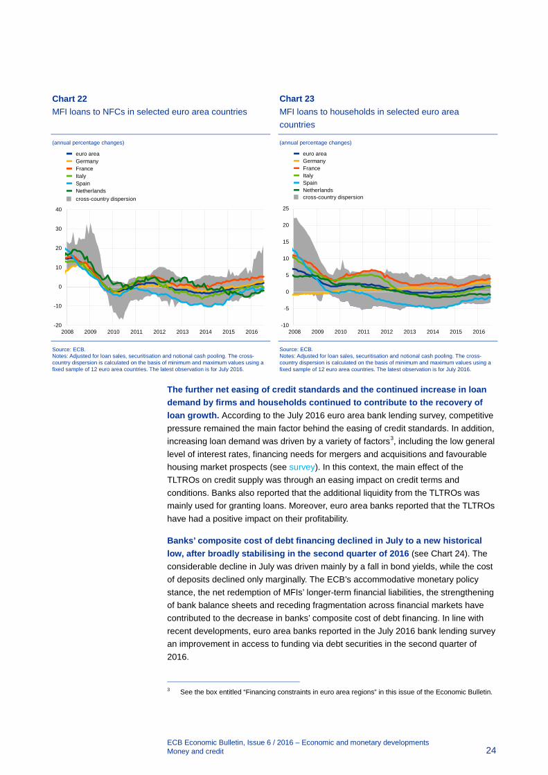
Loan dynamics continued to recover gradually. The annual growth rate of MFI loans to the private sector (adjusted for loan sales, securitisation and notional cash pooling) increased further in the second quarter of 2016 and in July (see Chart 20). Loan growth improved during this period, particularly for non-financial corporations (see Chart 22), having recovered substantially from the trough of the first quarter of 2014. This improvement is broadly shared by the largest countries, though loan growth rates are still negative in some jurisdictions. In comparison, the annual growth rate of loans to households picked up slightly in the second quarter of 2016 and remained unchanged in July (see Chart 23). The significant decreases in bank lending rates seen across the euro area since summer 2014 (notably owing to the ECB’s non-standard monetary policy measures) and improvements in the supply of, and demand for, bank loans have supported these trends. However, the ongoing consolidation of bank balance sheets and still high levels of non-performing loans in some countries continue to curb loan growth.
ECB Economic Bulletin, Issue 6 / 2016 – Economic and monetary developments Money and credit 24
Chart 23 MFI loans to households in selected euro area countries
(annual percentage changes)
Source: ECB. Notes: Adjusted for loan sales, securitisation and notional cash pooling. The cross-country dispersion is calculated on the basis of minimum and maximum values using a fixed sample of 12 euro area countries. The latest observation is for July 2016.
The further net easing of credit standards and the continued increase in loan demand by firms and households continued to contribute to the recovery of loan growth. According to the July 2016 euro area bank lending survey, competitive pressure remained the main factor behind the easing of credit standards. In addition, increasing loan demand was driven by a variety of factors3, including the low general level of interest rates, financing needs for mergers and acquisitions and favourable housing market prospects (see survey). In this context, the main effect of the TLTROs on credit supply was through an easing impact on credit terms and conditions. Banks also reported that the additional liquidity from the TLTROs was mainly used for granting loans. Moreover, euro area banks reported that the TLTROs have had a positive impact on their profitability.
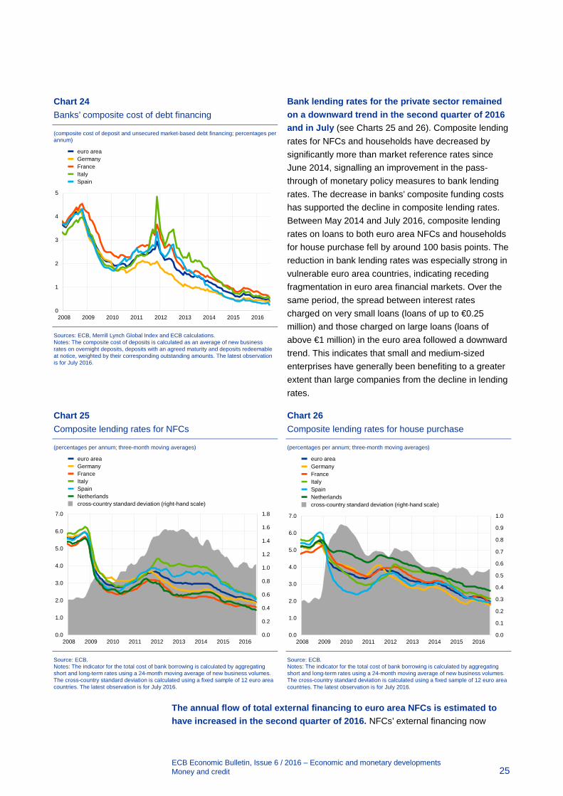
Banks’ composite cost of debt financing declined in July to a new historical low, after broadly stabilising in the second quarter of 2016 (see Chart 24). The considerable decline in July was driven mainly by a fall in bond yields, while the cost of deposits declined only marginally. The ECB’s accommodative monetary policy stance, the net redemption of MFIs’ longer-term financial liabilities, the strengthening of bank balance sheets and receding fragmentation across financial markets have contributed to the decrease in banks’ composite cost of debt financing. In line with recent developments, euro area banks reported in the July 2016 bank lending survey an improvement in access to funding via debt securities in the second quarter of 2016.
3 See the box entitled “Financing constraints in euro area regions” in this issue of the Economic Bulletin.
-10
-5
0
5
10
15
20
25
2008 2009 2010 2011 2012 2013 2014 2015 2016
euro areaGermanyFranceItalySpainNetherlandscross-country dispersion
Chart 22 MFI loans to NFCs in selected euro area countries
(annual percentage changes)
Source: ECB. Notes: Adjusted for loan sales, securitisation and notional cash pooling. The cross-country dispersion is calculated on the basis of minimum and maximum values using a fixed sample of 12 euro area countries. The latest observation is for July 2016.
-20
-10
0
10
20
30
40
2008 2009 2010 2011 2012 2013 2014 2015 2016
euro areaGermanyFranceItalySpainNetherlandscross-country dispersion
ECB Economic Bulletin, Issue 6 / 2016 – Economic and monetary developments Money and credit 25
Bank lending rates for the private sector remained on a downward trend in the second quarter of 2016 and in July (see Charts 25 and 26). Composite lending rates for NFCs and households have decreased by significantly more than market reference rates since June 2014, signalling an improvement in the pass-through of monetary policy measures to bank lending rates. The decrease in banks’ composite funding costs has supported the decline in composite lending rates. Between May 2014 and July 2016, composite lending rates on loans to both euro area NFCs and households for house purchase fell by around 100 basis points. The reduction in bank lending rates was especially strong in vulnerable euro area countries, indicating receding fragmentation in euro area financial markets. Over the same period, the spread between interest rates charged on very small loans (loans of up to €0.25 million) and those charged on large loans (loans of above €1 million) in the euro area followed a downward trend. This indicates that small and medium-sized enterprises have generally been benefiting to a greater extent than large companies from the decline in lending rates.
Chart 26 Composite lending rates for house purchase
(percentages per annum; three-month moving averages)
Source: ECB. Notes: The indicator for the total cost of bank borrowing is calculated by aggregating short and long-term rates using a 24-month moving average of new business volumes. The cross-country standard deviation is calculated using a fixed sample of 12 euro area countries. The latest observation is for July 2016.
The annual flow of total external financing to euro area NFCs is estimated to have increased in the second quarter of 2016. NFCs’ external financing now
0.0
0.1
0.2
0.3
0.4
0.5
0.6
0.7
0.8
0.9
1.0
0.0
1.0
2.0
3.0
4.0
5.0
6.0
7.0
2008 2009 2010 2011 2012 2013 2014 2015 2016
euro areaGermanyFranceItalySpainNetherlandscross-country standard deviation (right-hand scale)
Chart 24 Banks’ composite cost of debt financing
(composite cost of deposit and unsecured market-based debt financing; percentages per annum)
Sources: ECB, Merrill Lynch Global Index and ECB calculations. Notes: The composite cost of deposits is calculated as an average of new business rates on overnight deposits, deposits with an agreed maturity and deposits redeemable at notice, weighted by their corresponding outstanding amounts. The latest observation is for July 2016.
Chart 25 Composite lending rates for NFCs
(percentages per annum; three-month moving averages)
Source: ECB. Notes: The indicator for the total cost of bank borrowing is calculated by aggregating short and long-term rates using a 24-month moving average of new business volumes. The cross-country standard deviation is calculated using a fixed sample of 12 euro area countries. The latest observation is for July 2016.
0
1
2
3
4
5
2008 2009 2010 2011 2012 2013 2014 2015 2016
euro areaGermany FranceItalySpain
0.0
0.2
0.4
0.6
0.8
1.0
1.2
1.4
1.6
1.8
0.0
1.0
2.0
3.0
4.0
5.0
6.0
7.0
2008 2009 2010 2011 2012 2013 2014 2015 2016
euro areaGermanyFranceItalySpainNetherlandscross-country standard deviation (right-hand scale)

ECB Economic Bulletin, Issue 6 / 2016 – Economic and monetary developments Money and credit 26
stands at levels seen at the end of 2004 (before the start of the period of excessive credit growth). The recovery in NFCs’ external financing observed since early 2014 has been supported by the strengthening of economic activity, further declines in the cost of bank lending, the easing of bank lending conditions, the very low cost of market-based debt and larger numbers of mergers and acquisitions. At the same time, NFCs’ record high cash holdings have reduced the need for external financing.
Net issuance of debt securities by euro area NFCs strengthened further in April and May 2016, before contracting in June. The strengthening in April and May was supported, among other factors, by the ECB’s monetary policy package announced in March 2016, including the corporate sector purchase programme, and was widespread across countries4. The June moderation was most likely related to concerns about the UK referendum. Available evidence suggests that corporate bond issuance strengthened modestly again in July and August. The net issuance of quoted shares by NFCs has remained fairly modest in recent months.
The overall nominal cost of external financing for euro area NFCs is estimated to have fallen in July 2016 to a new historical low, before returning in August to the levels observed in the second quarter of 2016. The July decline was due both to a fall in the cost of equity financing and to a decline in the cost of market-based debt financing, while the increase in August was attributable exclusively to a rise in the cost of equity financing. The cost of equity financing followed developments in equity prices and expected earnings. The cost of market-based debt financing continued to decline over the period from June to August as a consequence of the ECB’s March 2016 monetary policy measures and globally declining yields.
4 See also the box entitled “The corporate bond market and the ECB’s corporate sector purchase
programme”, Economic Bulletin, Issue 5, ECB, 2016.

ECB Economic Bulletin, Issue 6 / 2016 – Economic and monetary developments Fiscal developments 27
6 Fiscal developments
The euro area budget deficit is foreseen to continue to decline over the projection horizon (2016-18) mainly on the back of lower interest payments and favourable cyclical conditions. The aggregate fiscal stance for the euro area is projected to be expansionary in 2016, but to turn broadly neutral in 2017-18. While the aggregate debt-to-GDP ratio is projected to decline over the projection horizon, this masks large cross-country differences. In particular, those countries with high debt levels would need additional consolidation efforts to set their public debt ratio firmly on a downward path, while other countries with fiscal space should use this room for budgetary manoeuvre to support demand.
The euro area general government budget deficit is projected to decline gradually over the projection horizon. Based on the September 2016 ECB staff macroeconomic projections5, the budget deficit is expected to decline from 2.1% of GDP in 2015 to 1.5% of GDP in 2018 (see the table). In 2016, lower interest payments together with favourable cyclical conditions are projected to more than offset the fiscal loosening. In 2017 and 2018, low interest payments are foreseen to remain an important driver of the deficit reduction. Compared with the June 2016 projections, the fiscal outlook remains broadly unchanged over the projection horizon.6 More detailed information on the 2017 budgets will only become available when the euro area countries submit their draft budgetary plans by mid-October.
The euro area fiscal stance is projected to be expansionary in 2016 and to turn broadly neutral in 2017 and 2018.7 The loosening of the aggregate fiscal stance in 2016 reflects the impact of expansionary measures on the revenue side, such as cuts in direct taxes and social security contributions in a number of euro area countries. The expansionary fiscal stance can be regarded as broadly appropriate in view of the need to find a balance between the amount of slack in the economy and the limited fiscal space, the latter in countries with high public debt. Regarding the period 2017-18, the fiscal stance is projected to be broadly neutral, as deficit-increasing measures on the revenue side are likely to be offset by less dynamically growing government primary expenditure items. The latter include, in particular, compensation of employees and intermediate consumption, which are projected to grow below nominal trend GDP growth, while other items, such as social transfers and government investment, are foreseen to grow above potential.
5 See the September 2016 ECB staff macroeconomic projections for the euro area, available at
https://www.ecb.europa.eu/pub/pdf/other/ecbstaffprojections201609.en.pdf 6 Preliminary estimates of the German government accounts only become available after the cut-off date.
The general government surplus recorded in the first half of 2016 was, at 1.2% of GDP, significantly higher than the balanced budget projected in the German stability programme for the full year. While the full-year figures are likely to be lower than the figures for the first half of 2016, a significant surplus is likely.
7 The fiscal stance is measured as the change in the structural primary balance, i.e. the cyclically adjusted primary balance net of temporary measures, such as government support to the financial sector. For a discussion of the concept of the euro area fiscal stance, see the article entitled “The euro area fiscal stance”, Economic Bulletin, Issue 4, ECB, 2016.

ECB Economic Bulletin, Issue 6 / 2016 – Economic and monetary developments Fiscal developments 28
Table Fiscal developments in the euro area
(percentages of GDP)
Sources: Eurostat, ECB and September 2016 ECB staff macroeconomic projections. Notes: The data refer to the aggregate general government sector of the euro area. Owing to rounding, figures may not add up. The slight variation from the validated Eurostat data from spring 2016 is due to recent data revisions, which have been taken into account in the September projections.
The high euro area government debt levels are expected to fall further. The euro area debt-to-GDP ratio, which peaked in 2014, is projected to decline gradually from 90.3% of GDP in 2015 to 87.0% of GDP by the end of 2018. The projected reduction in government debt is supported by various factors, including favourable developments in the interest rate-growth differential as a result of the better macroeconomic outlook and assumed low interest rates. Small primary surpluses and negative deficit-debt adjustments will also contribute to a better debt outlook. Compared with the June 2016 projections, the euro area debt-to-GDP ratio is expected to be somewhat lower by the end of the projection horizon, which notably relates to the strong upward revision to Irish nominal GDP for 2015.8 From a cross-country perspective, the debt-to-GDP ratio is foreseen to remain heterogeneous, with more than half of euro area countries exceeding the 60% threshold by the end of the projection horizon. Moreover, in a few countries, the government debt ratio is expected to increase further over the projection horizon.
Further consolidation efforts are essential, notably in countries with high debt-to-GDP ratios. These countries need to set their public debt ratio firmly on a downward path, as they are particularly vulnerable to renewed financial market instability or a rebound in interest rates. Euro area countries with fiscal space should, in turn, make use of the room for manoeuvre, for example by expanding public investment, while all countries should strive for a more growth-enhancing composition of government budgets.
Full compliance with the Stability and Growth Pact would support countries in correcting budgetary imbalances and thus guide them towards an appropriate debt trajectory. In this regard, on 12 July the Ecofin Council concurred with the
8 As a result of the upward revision to Irish nominal GDP for 2015, the euro area debt-to-GDP ratio
declined by roughly 0.4 percentage point.
2013 2014 2015 2016 2017 2018
a. Total revenue 46.6 46.7 46.4 45.9 45.7 45.7
b. Total expenditure 49.6 49.3 48.4 47.8 47.4 47.1
of which:
c. Interest expenditure 2.8 2.6 2.4 2.2 2.0 1.9
d. Primary expenditure (b - c) 46.8 46.7 46.1 45.7 45.4 45.3
Budget balance (a - b) -3.0 -2.6 -2.1 -1.9 -1.7 -1.5
Primary budget balance (a - d) -0.2 0.1 0.3 0.2 0.3 0.4
Cyclically adjusted budget balance -2.2 -1.9 -1.7 -2.0 -1.8 -1.6
Structural balance -2.2 -1.7 -1.6 -1.9 -1.8 -1.6
Gross debt 91.1 92.0 90.3 89.5 88.4 87.0
Memo item: real GDP (percentage changes) -0.2 1.1 1.9 1.7 1.6 1.6

ECB Economic Bulletin, Issue 6 / 2016 – Economic and monetary developments Fiscal developments 29
Commission assessment that neither Portugal nor Spain had taken effective action to correct their excessive deficits by the respective deadlines of 2015 and 2016. On 2 August the Council therefore gave notice on the measures needed to be taken to correct the excessive deficit. It recommended Portugal to correct its excessive deficit this year, based on an additional fiscal effort of 0.25% of GDP, and to reduce the headline budget deficit to 2.5% of GDP. In turn, Spain was granted a two-year deadline extension to 2018, associated with a deterioration in the structural deficit of 0.4% of GDP this year and structural annual improvements of 0.5% of GDP thereafter. Both countries are invited to outline their plans on how they intend to follow up on the Council’s recommendations by 15 October. Despite the assessment that no effective action had been taken by either country, on 8 August the Council followed the Commission recommendation not to impose sanctions, which in principle should automatically apply in the event of continued non-compliance with the Pact (as introduced with the “six-pack” regulations in 2011). In an upcoming structured dialogue with the European Parliament, the Commission will outline its recommendation regarding the usage of its tool to suspend part of the structural funds in the light of Portugal’s and Spain’s non-compliance with the Pact.
Looking ahead, efforts will need to be made to ensure that the draft budgetary plans are an effective early warning and correction tool. This requires that the provisions of the “two-pack” regulations are fully and consistently applied across time and countries. Following the submission of the draft budgetary plans in mid-October, the Commission will assess whether they are in full compliance with the requirements of the Pact. In the event of non-compliance, the Commission will have to send the draft budgetary plans back to the countries concerned.

ECB Economic Bulletin, Issue 6 / 2016 – Boxes Determinants of the slowdown in global trade: what is the new normal? 30
Boxes
1 Determinants of the slowdown in global trade: what is the new normal?
Global trade has been exceptionally weak over the past five years. Annual world import growth has been below its long-run average since mid-2011, the longest period of below-trend growth for half a century. Prior to the Great Recession, global trade grew on average roughly twice as fast as global output; since 2012 trade has barely matched the growth rates of world GDP (see Chart A). As a result, the global imports-to-GDP ratio has discontinued its strong upward trend and largely stagnated in the past five years (see Chart B). The observed decline in the gross income elasticity of trade – defined as the average growth rate of world imports divided by the average growth rate of world GDP – raises the question whether the trade weakness represents a temporary deviation from trend or a longer-lasting phenomenon reflecting more fundamental structural changes. The question has been a prominent area of recent research9 and is highly relevant for central banks seeking to understand the role of external demand and international linkages in shaping the outlook for domestic activity, potential output and inflation. A recent report by experts of the European System of Central Banks (ESCB) finds that the weakness in world trade relative to global GDP is likely to persist, being mainly driven by two developments.10
9 See, for instance, Hoekman, B., “The Global Trade Slowdown: A New Normal?”, VoxEU.org eBook,
CEPR Press and EUI, London, 2015; ECB, “Understanding the weakness in world trade”, Economic Bulletin, Issue 3, 2015; Borin, A. and Mancini, M., “Follow the value added: bilateral gross export accounting”, Working Paper, No 1026, Banca d’Italia, 2015.
10 IRC Trade Task Force, “Understanding the weakness in global trade: what is the new normal?”, Occasional Paper Series, No 178, ECB, September 2016. In the report, global GDP is aggregated at market exchange rate weights, whereas in this box global GDP is aggregated at purchasing power parity (PPP) weights to align the results more closely with the Eurosystem staff projections of world GDP.
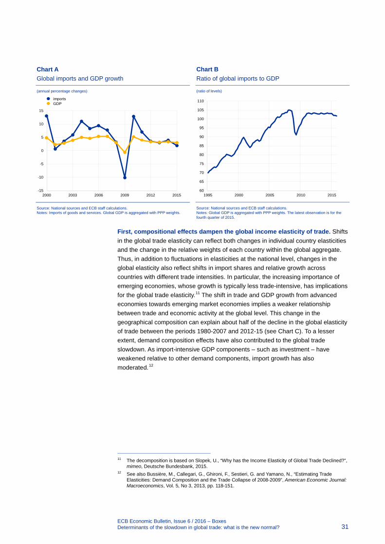
ECB Economic Bulletin, Issue 6 / 2016 – Boxes Determinants of the slowdown in global trade: what is the new normal? 31
Chart B Ratio of global imports to GDP
(ratio of levels)
Source: National sources and ECB staff calculations. Notes: Global GDP is aggregated with PPP weights. The latest observation is for the fourth quarter of 2015.
First, compositional effects dampen the global income elasticity of trade. Shifts in the global trade elasticity can reflect both changes in individual country elasticities and the change in the relative weights of each country within the global aggregate. Thus, in addition to fluctuations in elasticities at the national level, changes in the global elasticity also reflect shifts in import shares and relative growth across countries with different trade intensities. In particular, the increasing importance of emerging economies, whose growth is typically less trade-intensive, has implications for the global trade elasticity.11 The shift in trade and GDP growth from advanced economies towards emerging market economies implies a weaker relationship between trade and economic activity at the global level. This change in the geographical composition can explain about half of the decline in the global elasticity of trade between the periods 1980-2007 and 2012-15 (see Chart C). To a lesser extent, demand composition effects have also contributed to the global trade slowdown. As import-intensive GDP components – such as investment – have weakened relative to other demand components, import growth has also moderated.12
11 The decomposition is based on Slopek, U., “Why has the Income Elasticity of Global Trade Declined?”,
mimeo, Deutsche Bundesbank, 2015. 12 See also Bussière, M., Callegari, G., Ghironi, F., Sestieri, G. and Yamano, N., “Estimating Trade
Elasticities: Demand Composition and the Trade Collapse of 2008-2009”, American Economic Journal: Macroeconomics, Vol. 5, No 3, 2013, pp. 118-151.
60
65
70
75
80
85
90
95
100
105
110
1995 2000 2005 2010 2015
Chart A Global imports and GDP growth
(annual percentage changes)
Source: National sources and ECB staff calculations. Notes: Imports of goods and services. Global GDP is aggregated with PPP weights.
-15
-10
-5
0
5
10
15
2000 2003 2006 2009 2012 2015
importsGDP
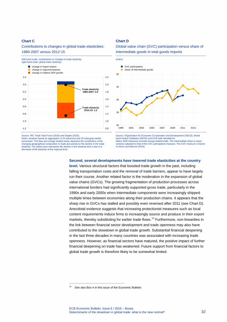
ECB Economic Bulletin, Issue 6 / 2016 – Boxes Determinants of the slowdown in global trade: what is the new normal? 32
Chart D Global value chain (GVC) participation versus share of intermediate goods in total goods imports
(index)
Source: Organisation for Economic Co-operation and Development (OECD), World Input-Output Database (WIOD) and ECB staff calculations. Notes: Both measures exclude energy-related trade. The intermediate share is mean-variance adjusted to that of the GVC participation measure. The GVC measure is based on Borin and Mancini (2015).
Second, several developments have lowered trade elasticities at the country level. Various structural factors that boosted trade growth in the past, including falling transportation costs and the removal of trade barriers, appear to have largely run their course. Another related factor is the moderation in the expansion of global value chains (GVCs). The growing fragmentation of production processes across international borders had significantly supported gross trade, particularly in the 1990s and early 2000s when intermediate components were increasingly shipped multiple times between economies along their production chains. It appears that the sharp rise in GVCs has stalled and possibly even reversed after 2011 (see Chart D). Anecdotal evidence suggests that increasing protectionist measures such as local content requirements induce firms to increasingly source and produce in their export markets, thereby substituting for earlier trade flows.13 Furthermore, non-linearities in the link between financial sector development and trade openness may also have contributed to the slowdown in global trade growth. Substantial financial deepening in the last three decades in many countries was associated with increasing trade openness. However, as financial sectors have matured, the positive impact of further financial deepening on trade has weakened. Future support from financial factors to global trade growth is therefore likely to be somewhat limited.
13 See also Box 4 in this issue of the Economic Bulletin.
30
35
40
45
50
1999 2001 2003 2005 2007 2009 2011 2013
GVC participationshare of intermediate goods
Chart C Contributions to changes in global trade elasticities: 1980-2007 versus 2012-15
(left-hand scale: contributions to changes in trade elasticity; right-hand scale: global trade elasticity)
Source: IRC Trade Task Force (2016) and Slopek (2015). Notes: Analysis based on aggregates of 24 advanced and 18 emerging market economies. The blue and orange shaded areas represent the contribution of the changing geographical composition in trade and activity to the decline in the trade elasticity. The yellow area represents the decline in the elasticity that is due to a decrease of the elasticity at the regional level.
0.8
1.0
1.2
1.4
1.6
1.8
2.0
2.2
-1.2
-1.0
-0.8
-0.6
-0.4
-0.2
0.0
0.2
Trade elasticity1980-2007: 2.0
Trade elasticity2012-15: 1.2
change in import shareschange in regional elasticitychange in relative GDP growth
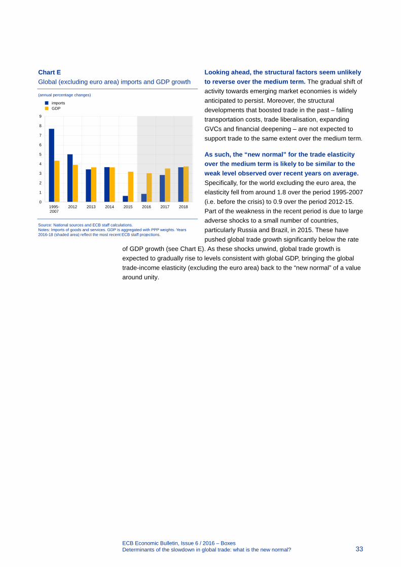
ECB Economic Bulletin, Issue 6 / 2016 – Boxes Determinants of the slowdown in global trade: what is the new normal? 33
Looking ahead, the structural factors seem unlikely to reverse over the medium term. The gradual shift of activity towards emerging market economies is widely anticipated to persist. Moreover, the structural developments that boosted trade in the past – falling transportation costs, trade liberalisation, expanding GVCs and financial deepening – are not expected to support trade to the same extent over the medium term.
As such, the “new normal” for the trade elasticity over the medium term is likely to be similar to the weak level observed over recent years on average. Specifically, for the world excluding the euro area, the elasticity fell from around 1.8 over the period 1995-2007 (i.e. before the crisis) to 0.9 over the period 2012-15. Part of the weakness in the recent period is due to large adverse shocks to a small number of countries, particularly Russia and Brazil, in 2015. These have pushed global trade growth significantly below the rate
of GDP growth (see Chart E). As these shocks unwind, global trade growth is expected to gradually rise to levels consistent with global GDP, bringing the global trade-income elasticity (excluding the euro area) back to the “new normal” of a value around unity.
Chart E Global (excluding euro area) imports and GDP growth
(annual percentage changes)
Source: National sources and ECB staff calculations. Notes: Imports of goods and services. GDP is aggregated with PPP weights. Years 2016-18 (shaded area) reflect the most recent ECB staff projections.
0
1
2
3
4
5
6
7
8
9
1995-2007
2012 2013 2014 2015 2016 2017 2018
importsGDP
ECB Economic Bulletin, Issue 6 / 2016 – Boxes Financing constraints in euro area regions 34
2 Financing constraints in euro area regions
This box presents new evidence on access to finance at regional level within the euro area. The Survey on Access to Finance of Enterprises (SAFE) has been carried out by the ECB and the European Commission since 2009 on a biannual basis. It provides information on developments in firms’ access to and use of external financing in the euro area, broken down by firm size and sector. Until now, analysis of the results of this survey has focused mainly on differences between euro area countries, disregarding heterogeneity at a regional level within countries. However, there is growing evidence that the regional dimension of access to finance is important even in integrated financial markets, particularly for small and medium-sized enterprises (SMEs). Indeed, the level of regional financial development – which often has important implications as regards the accessibility of external sources of finance – is positively correlated with growth at a regional level. At the same time, regional market conditions matter in terms of determining financing constraints that are not related to firms’ individual financial characteristics and circumstances.14
Financing constraints vary from region to region across the euro area. Since April 2014, information on the regions where surveyed companies are located has been collected by the SAFE survey on the basis of level 1 of the Nomenclature of Territorial Units for Statistics (NUTS). Thus, the 12 euro area countries covered by the survey are broken down into 57 major socio-economic regions.15 Chart A shows the level of financing constraints in these various regions by firm size, based on survey results from 2014 to 2016.16 Under the definition used in the survey, a firm is considered to be financially constrained if it applies for a bank loan or credit line and its application is rejected (or accepted only in part) or it refuses the loan or credit line on offer because the associated costs are too high. A firm is also considered to face financing constraints if it needs a bank loan or credit line but is discouraged from applying for one. The percentage of firms that have experienced financing constraints appears to vary from region to region within individual countries. In addition, smaller companies appear to be more likely to experience financing constraints in most regions, with more pronounced regional differences relative to larger companies.
14 See Guiso, L., Sapienza, P. and Zingales, L., “Does local financial development matter?”, Quarterly
Journal of Economics, Vol. 119, 2004, pp. 929-969, and Deloof, M. and La Rocca, M., “Local financial development and the trade credit policy of Italian SMEs”, Small Business Economics, Vol. 44, 2015, pp. 905-924.
15 The countries in question are Belgium (3 regions), Germany (16 regions), Ireland (1 region), Greece (4 regions), Spain (7 regions), France (9 regions), Italy (5 regions), the Netherlands (4 regions), Austria (3 regions), Portugal (3 regions), Slovakia (1 region) and Finland (1 region).
16 Figures in the charts in this box are weighted using the calibration scheme employed by the survey. See www.ecb.europa.eu/stats/pdf/surveys/sme/methodological_information_survey_and_user_guide.pdf for an explanation of the weights used. The same weights are used in the regression analyses.
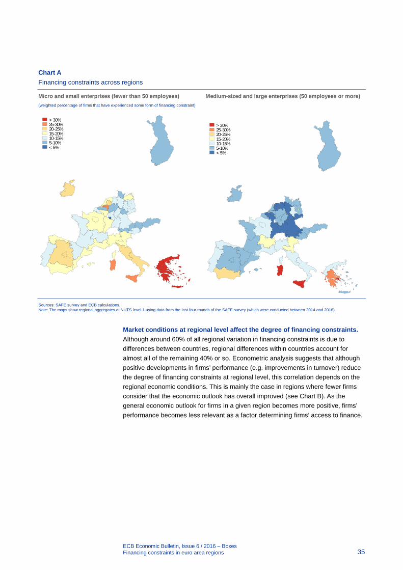
ECB Economic Bulletin, Issue 6 / 2016 – Boxes Financing constraints in euro area regions 35
Chart A Financing constraints across regions
Micro and small enterprises (fewer than 50 employees) Medium-sized and large enterprises (50 employees or more) (weighted percentage of firms that have experienced some form of financing constraint)
Sources: SAFE survey and ECB calculations. Note: The maps show regional aggregates at NUTS level 1 using data from the last four rounds of the SAFE survey (which were conducted between 2014 and 2016).
Market conditions at regional level affect the degree of financing constraints. Although around 60% of all regional variation in financing constraints is due to differences between countries, regional differences within countries account for almost all of the remaining 40% or so. Econometric analysis suggests that although positive developments in firms’ performance (e.g. improvements in turnover) reduce the degree of financing constraints at regional level, this correlation depends on the regional economic conditions. This is mainly the case in regions where fewer firms consider that the economic outlook has overall improved (see Chart B). As the general economic outlook for firms in a given region becomes more positive, firms’ performance becomes less relevant as a factor determining firms’ access to finance.
> 30%25-30%20-25%15-20%10-15%5-10%< 5%
> 30%25-30%20-25%15-20%10-15%5-10%< 5%
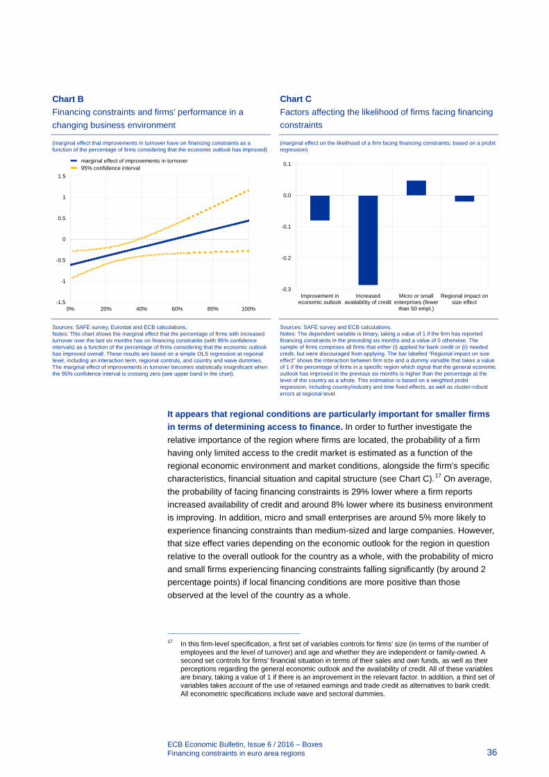
ECB Economic Bulletin, Issue 6 / 2016 – Boxes Financing constraints in euro area regions 36
Chart C Factors affecting the likelihood of firms facing financing constraints
(marginal effect on the likelihood of a firm facing financing constraints; based on a probit regression)
Sources: SAFE survey and ECB calculations. Notes: The dependent variable is binary, taking a value of 1 if the firm has reported financing constraints in the preceding six months and a value of 0 otherwise. The sample of firms comprises all firms that either (i) applied for bank credit or (ii) needed credit, but were discouraged from applying. The bar labelled “Regional impact on size effect” shows the interaction between firm size and a dummy variable that takes a value of 1 if the percentage of firms in a specific region which signal that the general economic outlook has improved in the previous six months is higher than the percentage at the level of the country as a whole. This estimation is based on a weighted probit regression, including country/industry and time fixed effects, as well as cluster-robust errors at regional level.
It appears that regional conditions are particularly important for smaller firms in terms of determining access to finance. In order to further investigate the relative importance of the region where firms are located, the probability of a firm having only limited access to the credit market is estimated as a function of the regional economic environment and market conditions, alongside the firm’s specific characteristics, financial situation and capital structure (see Chart C).17 On average, the probability of facing financing constraints is 29% lower where a firm reports increased availability of credit and around 8% lower where its business environment is improving. In addition, micro and small enterprises are around 5% more likely to experience financing constraints than medium-sized and large companies. However, that size effect varies depending on the economic outlook for the region in question relative to the overall outlook for the country as a whole, with the probability of micro and small firms experiencing financing constraints falling significantly (by around 2 percentage points) if local financing conditions are more positive than those observed at the level of the country as a whole.
17 In this firm-level specification, a first set of variables controls for firms’ size (in terms of the number of
employees and the level of turnover) and age and whether they are independent or family-owned. A second set controls for firms’ financial situation in terms of their sales and own funds, as well as their perceptions regarding the general economic outlook and the availability of credit. All of these variables are binary, taking a value of 1 if there is an improvement in the relevant factor. In addition, a third set of variables takes account of the use of retained earnings and trade credit as alternatives to bank credit. All econometric specifications include wave and sectoral dummies.
-0.3
-0.2
-0.1
0.0
0.1
Improvement ineconomic outlook
Increasedavailability of credit
Micro or smallenterprises (fewer
than 50 empl.)
Regional impact onsize effect
Chart B Financing constraints and firms’ performance in a changing business environment
(marginal effect that improvements in turnover have on financing constraints as a function of the percentage of firms considering that the economic outlook has improved)
Sources: SAFE survey, Eurostat and ECB calculations. Notes: This chart shows the marginal effect that the percentage of firms with increased turnover over the last six months has on financing constraints (with 95% confidence intervals) as a function of the percentage of firms considering that the economic outlook has improved overall. These results are based on a simple OLS regression at regional level, including an interaction term, regional controls, and country and wave dummies. The marginal effect of improvements in turnover becomes statistically insignificant when the 95% confidence interval is crossing zero (see upper band in the chart).
-1.5
-1
-0.5
0
0.5
1
1.5
0% 20% 40% 60% 80% 100%
marginal effect of improvements in turnover95% confidence interval

ECB Economic Bulletin, Issue 6 / 2016 – Boxes Financing constraints in euro area regions 37
Overall, firm-level survey data confirm that regional market conditions affect the financing constraints faced by firms. Greater attention needs to be paid to determinants of regional differences in the availability of credit, looking at whether these are predominantly related to the nature of the local banking sector (i.e. its level of development) or local borrowers’ liquidity preferences.18 Ultimately, the use of such local information will provide additional guidance regarding the impact that monetary policy has in the various regions of the euro area.
18 See Rodríguez-Fuentes, C.J. and Dow, S.C., “EMU and the Regional Impact of Monetary Policy”,
Regional Studies, Vol. 37(9), 2003, pp. 969-980.
ECB Economic Bulletin, Issue 6 / 2016 – Boxes Liquidity conditions and monetary policy operations in the period from 27 April to 26 July 2016 38
3 Liquidity conditions and monetary policy operations in the period from 27 April to 26 July 2016
This box describes the ECB’s monetary policy operations during the third and fourth reserve maintenance periods of 2016, which ran from 27 April to 7 June and from 8 June to 26 July respectively. During this period the interest rates on the main refinancing operations (MROs), the marginal lending facility and the deposit facility remained unchanged at 0.00%, 0.25% and -0.40% respectively. On 28 June the first targeted longer-term refinancing operation (TLTRO) in the second series of TLTROs (TLTRO-II) was settled for an amount of €399.3 billion. However, that amount was largely offset by simultaneous voluntary repayments from the first series of TLTROs (TLTRO-I) totalling €367.9 billion. That voluntary repayment option allowed banks to switch from TLTRO-I to TLTRO-II, thereby benefiting from more favourable conditions. For example, the interest rate applied to TLTRO-II operations is linked to participating banks’ lending patterns – i.e. the more loans banks issue to non-financial corporations and households, the lower the interest rate on their TLTRO-II borrowing will be.19 On 28 June the eighth and final TLTRO-I operation was settled for €6.7 billion, compared with €7.3 billion in the seventh TLTRO-I operation in March. Those voluntary repayments and new operations resulted in the total outstanding amount for both TLTRO programmes standing at €463.0 billion at the end of the review period. In addition, the Eurosystem continued buying public sector securities, covered bonds and asset-backed securities, and started to purchase corporate sector securities as part of its expanded asset purchase programme (APP),20 with a target of €80 billion of purchases per month.
Liquidity needs
In the period under review, the average daily liquidity needs of the banking system, defined as the sum of autonomous factors and reserve requirements, stood at €843.1 billion, an increase of €64.5 billion compared with the previous review period (i.e. the first and second maintenance periods of 2016). That increase in liquidity needs was attributable almost exclusively to an increase in average net autonomous factors, which rose by €63.1 billion to stand at €727.6 billion (see table).
19 For further information on TLTRO-II operations, see the box entitled “The second series of targeted
longer-term refinancing operations (TLTRO-II)”, Economic Bulletin, Issue 3, ECB, 2016. 20 Detailed information on the APP is available on the ECB’s website.
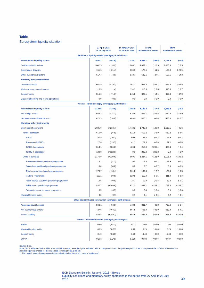
ECB Economic Bulletin, Issue 6 / 2016 – Boxes Liquidity conditions and monetary policy operations in the period from 27 April to 26 July 2016 39
Table Eurosystem liquidity situation
Source: ECB. Note: Since all figures in the table are rounded, in some cases the figure indicated as the change relative to the previous period does not represent the difference between the rounded figures provided for these periods (differing by €0.1 billion). 1) The overall value of autonomous factors also includes “items in course of settlement”.
27 April 2016
to 26 July 2016 27 January 2016 to 26 April 2016
Fourth maintenance period
Third maintenance period
Liabilities – liquidity needs (averages; EUR billions)
Autonomous liquidity factors 1,851.7 (+81.6) 1,770.1 1,897.7 (+99.8) 1,797.9 (-1.9)
Banknotes in circulation 1,082.3 (+16.2) 1,066.1 1,087.1 (+10.5) 1,076.6 (+7.3)
Government deposits 151.6 (+21.4) 130.3 175.5 (+51.6) 123.9 (-23.5)
Other autonomous factors 617.7 (+44.0) 573.7 635.1 (+37.6) 597.5 (+14.3)
Monetary policy instruments
Current accounts 641.9 (+79.2) 562.7 657.5 (+33.7) 623.8 (+53.8)
Minimum reserve requirements 115.5 (+1.4) 114.1 115.9 (+0.8) 115.0 (+0.7)
Deposit facility 316.6 (+71.6) 245.0 323.1 (+14.1) 309.0 (+47.0)
Liquidity-absorbing fine-tuning operations 0.0 (+0.0) 0.0 0.0 (+0.0) 0.0 (+0.0)
Assets – liquidity supply (averages; EUR billions)
Autonomous liquidity factors 1,124.5 (+18.6) 1,105.9 1,132.3 (+17.0) 1,115.3 (+2.3)
Net foreign assets 654.2 (+37.3) 616.8 666.1 (+25.8) 640.3 (+13.0)
Net assets denominated in euro 470.3 (-18.8) 489.0 466.2 (-8.8) 475.0 (-10.7)
Monetary policy instruments
Open market operations 1,685.9 (+213.7) 1,472.2 1,746.3 (+130.8) 1,615.5 (+96.6)
Tender operations 515.0 (-6.8) 521.9 519.2 (+8.9) 510.2 (-8.6)
MROs 50.5 (-10.2) 60.6 47.6 (-6.3) 53.9 (-4.2)
Three-month LTROs 27.6 (-13.5) 41.1 24.5 (-6.6) 31.1 (-6.8)
TLTRO-I operations 314.1 (-106.0) 420.2 218.9 (-206.4) 425.3 (+2.4)
TLTRO-II operations 122.9 (+122.9) 0.0 228.2 (+228.2) 0.0 (+0.0)
Outright portfolios 1,170.9 (+220.6) 950.3 1,227.1 (+121.9) 1,105.3 (+105.2)
First covered bond purchase programme 18.3 (-1.2) 19.5 17.8 (-1.1) 18.9 (-0.3)
Second covered bond purchase programme 8.0 (-0.8) 8.8 7.7 (-0.7) 8.4 (-0.3)
Third covered bond purchase programme 179.7 (+18.4) 161.3 183.3 (+7.7) 175.6 (+8.5)
Markets Programme 111.1 (-9.6) 120.8 110.9 (-0.5) 111.4 (-8.3)
Asset-backed securities purchase programme 19.5 (+0.8) 18.7 19.9 (+0.8) 19.0 (-0.1)
Public sector purchase programme 830.7 (+209.6) 621.2 881.1 (+109.1) 772.0 (+105.7)
Corporate sector purchase programme 3.5 (+3.5) 0.0 6.4 (+6.4) 0.0 (+0.0)
Marginal lending facility 0.2 (+0.1) 0.1 0.1 (-0.1) 0.2 (+0.1)
Other liquidity-based information (averages; EUR billions)
Aggregate liquidity needs 843.1 (+64.5) 778.6 881.7 (+83.8) 798.0 (-3.4)
Net autonomous factors1 727.6 (+63.1) 664.5 765.9 (+82.9) 682.9 (-4.1)
Excess liquidity 842.8 (+149.2) 693.6 864.5 (+47.0) 817.5 (+100.0)
Interest rate developments (averages; percentages)
MROs 0.00 (-0.03) 0.03 0.00 (+0.00) 0.00 (+0.00)
Marginal lending facility 0.25 (-0.03) 0.28 0.25 (+0.00) 0.25 (+0.00)
Deposit facility -0.40 (-0.05) -0.35 -0.40 (+0.00) -0.40 (+0.00)
EONIA -0.333 (-0.048) -0.286 -0.330 (+0.007) -0.337 (+0.003)
ECB Economic Bulletin, Issue 6 / 2016 – Boxes Liquidity conditions and monetary policy operations in the period from 27 April to 26 July 2016 40
The increase in autonomous factors was mainly a result of an increase in liquidity-absorbing factors. The main contributor to this increase was government deposits, which increased on average by €21.4 billion to stand at €151.6 billion in the period under review. This increase stemmed from the fourth maintenance period, when the pronounced tax receipts seen in a number of euro area countries in June resulted in inflows to governments’ accounts with national central banks. This, coupled with the reluctance of some treasuries to place their excess liquidity in the market at negative rates, contributed to higher levels of government deposits being held with national central banks. Average demand for banknotes also increased, rising by €16.2 billion to stand at €1,082.3 billion. Other autonomous factors rose by €44.0 billion, more than government deposits and banknotes combined, but that increase was largely attributable to quarterly revaluations of portfolio positions and was therefore offset by changes to net foreign assets.
Liquidity-providing factors increased over the review period as the continuing decline in net assets denominated in euro was compensated for by an increase in net foreign assets. Average net assets denominated in euro fell to €470.3 billion, down €18.8 billion from the previous review period, on account of a decline in financial assets held by the Eurosystem for purposes other than monetary policy, together with an increase in liabilities held by foreign official institutions with the national central banks. Those institutions increased their holdings, despite the further reduction in the deposit facility rate, possibly because there were few attractive alternatives in the market. Net foreign assets increased by €37.3 billion to stand at €654.2 billion, mainly as a result of quarterly portfolio revaluations.
The volatility of autonomous factors remained elevated, broadly unchanged from the previous review period. That volatility primarily reflected strong fluctuations in government deposits and, to some extent, the quarterly revaluation of net foreign assets and net assets denominated in euro. Meanwhile, autonomous factors continued to rise. At the same time, the average absolute error in weekly forecasts of autonomous factors declined by €0.8 billion to stand at €5.2 billion in the period under review.
Liquidity provided through monetary policy instruments
The average amount of liquidity provided through open market operations – both tender operations and the asset purchase programme – increased by €213.7 billion to stand at €1,685.9 billion (see chart). This increase was entirely due to the ECB’s expanded asset purchase programme.

ECB Economic Bulletin, Issue 6 / 2016 – Boxes Liquidity conditions and monetary policy operations in the period from 27 April to 26 July 2016 41
The average amount of liquidity provided through tender operations declined slightly in the period under review, falling by €6.8 billion to stand at €515.0 billion. The increase in the liquidity provided by the TLTROs was more than offset by a decrease in the liquidity supplied via regular operations. More specifically, liquidity provided via MROs and three-month LTROs decreased by €10.2 billion and €13.5 billion respectively, while the outstanding amount of TLTROs increased by €16.9 billion as a net effect of the settlement of the first TLTRO-II operation and voluntary repayments from the first seven TLTRO-I operations.
Average liquidity provided through the expanded asset purchase programme increased by €220.6 billion to stand at €1,170.9 billion, mainly on account of the public sector purchase programme. Average liquidity provided by the public sector purchase
programme, the third covered bond purchase programme, the asset-backed securities purchase programme and the corporate sector purchase programme rose by €209.6 billion, €18.4 billion, €0.8 billion and €3.5 billion respectively. The redemption of bonds held under the Securities Markets Programme and the previous two covered bond purchase programmes totalled €11.6 billion.
Excess liquidity
As a consequence of the developments detailed above, excess liquidity rose on average by €149.2 billion to stand at €842.8 billion in the period under review (see chart). The majority of that increase came in the third maintenance period, when excess liquidity rose by €100.0 billion on account of increased purchases and a liquidity-providing effect resulting from changes in autonomous factors. The relatively small increase in excess liquidity in the fourth maintenance period was mainly a consequence of the larger rise in autonomous factors, which partially absorbed the increased liquidity provided by the expanded asset purchase programme.
That increase in excess liquidity was reflected mainly in higher average current account holdings, which rose by €79.2 billion to stand at €641.9 billion in the period under review. Average recourse to the deposit facility increased by €71.6 billion to stand at €316.6 billion.
Interest rate developments
Overnight money market rates remained close to the deposit facility rate in the review period. In the unsecured market, the EONIA (euro overnight index average)
Chart Evolution of monetary policy instruments and excess liquidity
(EUR billions)
Source: ECB.
0
200
400
600
800
1,000
1,200
1,400
1,600
1,800
2,000
07/14 10/14 01/15 04/15 07/15 10/15 01/16 04/16
tender operationsoutright portfoliosexcess liquidity

ECB Economic Bulletin, Issue 6 / 2016 – Boxes Liquidity conditions and monetary policy operations in the period from 27 April to 26 July 2016 42
averaged -0.333%, down from an average of -0.286% in the previous review period. The EONIA hovered within a narrow range, reaching a historical low of -0.356% on 26 May, but it also exhibited the usual spike at the end of the quarter, when it stood at -0.293%. Furthermore, average overnight repo rates in the GC Pooling market21 declined to -0.396% and -0.387% for the standard and extended collateral baskets respectively, down 0.064 percentage point and 0.066 percentage point respectively relative to the previous review period.
21 The GC Pooling market allows repurchase agreements to be traded on the Eurex platform against
standardised baskets of collateral.
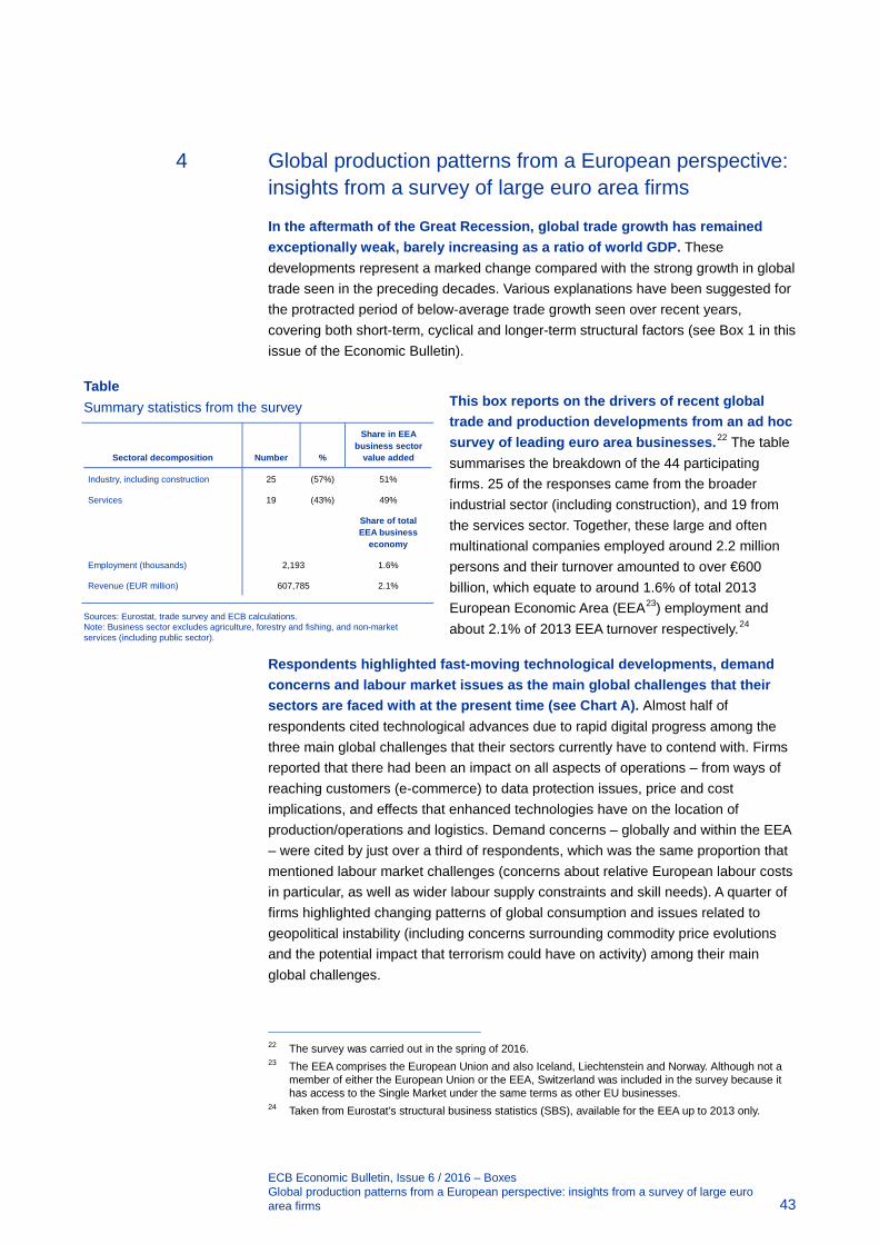
ECB Economic Bulletin, Issue 6 / 2016 – Boxes Global production patterns from a European perspective: insights from a survey of large euro area firms 43
4 Global production patterns from a European perspective: insights from a survey of large euro area firms
In the aftermath of the Great Recession, global trade growth has remained exceptionally weak, barely increasing as a ratio of world GDP. These developments represent a marked change compared with the strong growth in global trade seen in the preceding decades. Various explanations have been suggested for the protracted period of below-average trade growth seen over recent years, covering both short-term, cyclical and longer-term structural factors (see Box 1 in this issue of the Economic Bulletin).
This box reports on the drivers of recent global trade and production developments from an ad hoc survey of leading euro area businesses.22 The table summarises the breakdown of the 44 participating firms. 25 of the responses came from the broader industrial sector (including construction), and 19 from the services sector. Together, these large and often multinational companies employed around 2.2 million persons and their turnover amounted to over €600 billion, which equate to around 1.6% of total 2013 European Economic Area (EEA23) employment and about 2.1% of 2013 EEA turnover respectively.24
Respondents highlighted fast-moving technological developments, demand concerns and labour market issues as the main global challenges that their sectors are faced with at the present time (see Chart A). Almost half of respondents cited technological advances due to rapid digital progress among the three main global challenges that their sectors currently have to contend with. Firms reported that there had been an impact on all aspects of operations – from ways of reaching customers (e-commerce) to data protection issues, price and cost implications, and effects that enhanced technologies have on the location of production/operations and logistics. Demand concerns – globally and within the EEA – were cited by just over a third of respondents, which was the same proportion that mentioned labour market challenges (concerns about relative European labour costs in particular, as well as wider labour supply constraints and skill needs). A quarter of firms highlighted changing patterns of global consumption and issues related to geopolitical instability (including concerns surrounding commodity price evolutions and the potential impact that terrorism could have on activity) among their main global challenges.
22 The survey was carried out in the spring of 2016. 23 The EEA comprises the European Union and also Iceland, Liechtenstein and Norway. Although not a
member of either the European Union or the EEA, Switzerland was included in the survey because it has access to the Single Market under the same terms as other EU businesses.
24 Taken from Eurostat’s structural business statistics (SBS), available for the EEA up to 2013 only.
Table Summary statistics from the survey
Sectoral decomposition Number %
Share in EEA business sector
value added
Industry, including construction 25 (57%) 51%
Services 19 (43%) 49%
Share of total EEA business
economy
Employment (thousands) 2,193 1.6%
Revenue (EUR million) 607,785 2.1%
Sources: Eurostat, trade survey and ECB calculations. Note: Business sector excludes agriculture, forestry and fishing, and non-market services (including public sector).

ECB Economic Bulletin, Issue 6 / 2016 – Boxes Global production patterns from a European perspective: insights from a survey of large euro area firms 44
Manufacturing firms in particular also highlighted the existence of trade barriers – including local content regulations, tariffs and customs duties, and the rise in less formal barriers (so-called “murky protectionism”) – as major concerns and impediments to economies of scale. Firms operating across several geographical jurisdictions highlighted the difficulties posed by the increasing incidence of “double” corporate taxation. In addition, respondents highlighted growing global competition in product markets, changing customer preferences and commodity price volatility as ongoing global challenges for their sectors. Financial constraints and concerns about maintaining access to finance were hardly mentioned.
Chart B Changes in local production over past five years
(percentage of responses)
Sources: Trade survey and ECB calculations. Notes: Responses to question: “Over the past five years, has it become more or less common for companies in your sector to produce/operate in the local markets in which goods and services are sold?”
The survey suggests that localisation of production closer to final markets has slightly increased over the past five years (see Chart B). Although most firms reported no changes to global production patterns over the past five years, just over a quarter of respondents reported having relocated production or service operations. Both changing global patterns of demand and high labour costs were cited as important factors driving operations out of the EEA. Local content requirements were also mentioned as an important driver. Other factors impacting on relocation decisions related to a desire to hedge against currency fluctuations, capacity constraints within the EEA, excessive regulation, and economic and political uncertainty.
Changes to global production patterns continue to reduce demand for EEA labour. Roughly twice as many firms considered that changes in global trade patterns had reduced demand for EEA labour in their sector as compared with those who saw increases. Declines were particularly strong among “blue collar” operatives (both in industry and services); however, demand was reported to have increased somewhat among the higher skilled occupations (including production technicians and supervisors or those in R&D and product design functions).
0%
10%
20%
30%
40%
50%
60%
70%
less unchanged more
industry and constructionservicesall respondents
Chart A Main global operational challenges at the present time
(percentage of responses, ranked from most frequently cited)
Sources: Trade survey and ECB calculations. Notes: Responses to question: “What are the three main global operational challenges in your sector at the present time? Please list at most three factors and briefly explain why these are important.”
0% 10% 20% 30% 40% 50%
technological issues
demand concerns
labour market challenges
changing global consumption
geopolitical instability
trade barriers
regulatory barriers
commodity price issues
overcapacity
growing global competition
price pressures
changing customer preference
exchange rate volatility
political uncertainty
other
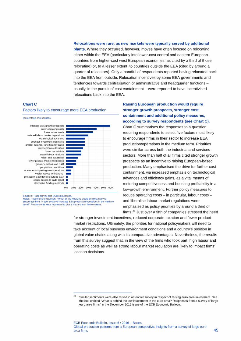
ECB Economic Bulletin, Issue 6 / 2016 – Boxes Global production patterns from a European perspective: insights from a survey of large euro area firms 45
Relocations were rare, as new markets were typically served by additional plants. Where they occurred, however, moves have often focused on relocating either within the EEA (particularly into lower-cost central and eastern European countries from higher-cost west European economies, as cited by a third of those relocating) or, to a lesser extent, to countries outside the EEA (cited by around a quarter of relocators). Only a handful of respondents reported having relocated back into the EEA from outside. Relocation incentives by some EEA governments and tendencies towards centralisation of administrative and headquarter functions – usually, in the pursuit of cost containment – were reported to have incentivised relocations back into the EEA.
Raising European production would require stronger growth prospects, stronger cost containment and additional policy measures, according to survey respondents (see Chart C). Chart C summarises the responses to a question requiring respondents to select five factors most likely to encourage firms in their sector to increase EEA production/operations in the medium term. Priorities were similar across both the industrial and services sectors. More than half of all firms cited stronger growth prospects as an incentive to raising European-based production. Many emphasised the drive for further cost containment, via increased emphasis on technological advances and efficiency gains, as a vital means of restoring competitiveness and boosting profitability in a low-growth environment. Further policy measures to reduce operating costs – in particular, labour costs – and liberalise labour market regulations were emphasised as policy priorities by around a third of firms.25 Just over a fifth of companies stressed the need
for stronger investment incentives, reduced corporate taxation and fewer product market restrictions. Ultimately, the priorities for national policymakers will need to take account of local business environment conditions and a country’s position in global value chains along with its comparative advantages. Nevertheless, the results from this survey suggest that, in the view of the firms who took part, high labour and operating costs as well as strong labour market regulation are likely to impact firms’ location decisions.
25 Similar sentiments were also raised in an earlier survey in respect of raising euro area investment. See
the box entitled “What is behind the low investment in the euro area? Responses from a survey of large euro area firms” in the December 2015 issue of the ECB Economic Bulletin.
Chart C Factors likely to encourage more EEA production
(percentage of responses)
Sources: Trade survey and ECB calculations. Notes: Responses to question: “Which of the following would be most likely to encourage firms in your sector to increase EEA production/operations in the medium term?” Respondents were requested to give a maximum of five elements.
0% 10% 20% 30% 40% 50% 60%
alternative funding methodseasier access to trade credit
protectionist tendencies outside EEAeasier access to financing
obstacles to opening new operationsgeopolitical conditions
greater emphasis on R&Dfewer product market restrictions
wider skill availabilityeased labour relations
lower uncertaintylower corporate taxation
greater potential for efficiency gainsstronger investment incentives
technological advancesreduced labour market regulations
lower labour costs lower operating costs
stronger EEA growth prospects
ECB Economic Bulletin, Issue 6 / 2016 – Boxes What accounts for the recent decoupling between the euro area GDP deflator and the HICP excluding energy and food? 46
5 What accounts for the recent decoupling between the euro area GDP deflator and the HICP excluding energy and food?
The GDP deflator can be seen as a broad indicator of underlying domestic price developments. There are some differences between the GDP deflator and the frequently used measure of HICP excluding energy and food regarding their concept and aim.26 Nevertheless, there has generally been a notable degree of co-movement between the longer-term developments of the two indicators. For the euro area, the average annual rate of increase in the past 15 years has been of relatively similar magnitude. Over the short to medium term, however, somewhat larger deviations between the two indicators are not uncommon, and the past two years are an example of a gap opening up: annual growth in the GDP deflator has increased more noticeably and has been rising since mid-2014, while HICP inflation excluding energy and food has edged up much less (see Chart A). This box explores the recent “decoupling” by looking specifically at factors that have accounted for the pick-up in the growth rate of the GDP deflator.
Developments in profit margins have been the main factor behind the recent acceleration in the euro area GDP deflator. A breakdown of growth in the GDP deflator into income components shows that almost all of the increase since mid-2014 is accounted for by higher contributions from profits (gross operating surplus) per unit of output, here referred to as profit margins. The contributions from unit labour costs and unit indirect taxes (net of subsidies) have on balance been roughly unchanged. Profit margin developments in the euro area are strongly procyclical and their recent strengthening is in line with the ongoing recovery in real GDP growth (see Chart B). Favourable developments in economic activity support profit margins as the improvements in income and demand facilitate price increases, and as the associated pick-up in productivity and the typically delayed response of wages to the cyclical upturn dampen unit labour costs. However, the impact of the economic cycle via profits should be a factor behind the developments in both the GDP deflator and the HICP excluding energy and food, suggesting that the recent decoupling reflects other factors.
26 The main conceptual differences between the two indicators result from the fact that the HICP
excluding energy and food refers to the prices of goods and services consumed by households, while the GDP deflator is more encompassing and captures the prices of all final products produced by the domestic economy. Looking at the GDP deflator from the expenditure side, it thus includes prices for private consumption, government consumption, capital formation and exports less those for imports. While prices for imported goods and services are not included in the GDP deflator, they are included in the HICP excluding energy and food (with the exception of the direct effect from energy and food prices). At the same time, the prices of exported goods and services are included in the GDP deflator, but obviously not in the HICP excluding energy and food.

ECB Economic Bulletin, Issue 6 / 2016 – Boxes What accounts for the recent decoupling between the euro area GDP deflator and the HICP excluding energy and food? 47
Chart B Real GDP and unit profits
(annual percentage changes)
Sources: Eurostat and ECB calculations.
Profit margins as captured in the GDP deflator have most likely recently also reflected changes in the terms of trade. This is suggested by a comparison of the decomposition of the GDP deflator on the income side with that on the expenditure side, where the former includes the profit margin and the latter includes the (relative) prices for exports and imports, i.e. the terms of trade. Changes in these terms may have recently reflected different factors. First, the depreciation of the effective exchange rate of the euro seen in mid-2014 could have benefited euro area exporters’ profit margins if they priced their products to the market, i.e. kept their export prices unchanged in the foreign currency. Second, the sharp fall in oil and other commodity prices in mid-2014 could have benefited euro area producers’ profit margins if they did not fully pass on the associated lower import and input prices to selling prices. Such an impact is suggested by the notable co-movement between the respective contributions of profit margins and the terms of trade to the growth rate of the GDP deflator in the past few years (see Chart C), while before cyclical developments appear to have dominated profit margin developments, as illustrated in Chart B.
The impact of input prices on profit margins helps to explain the recent gap between growth in the GDP deflator and that in the HICP excluding energy and food. The large fall in the price of oil reduced the price of inputs and intermediate consumption in production. Since intermediate consumption is not included in GDP, the change in oil input prices will not be directly mapped into the GDP deflator. At the same time, if the fall in oil input prices is at least partly passed on to selling prices as measured by final consumer prices, HICP inflation excluding energy and food may decline. By contrast, if the fall in oil input prices is not passed on to selling prices, HICP inflation excluding energy and food remains constant, whereas the GDP deflator increases (via higher profit margins). Chart D shows that the recent large differences between the growth rates of the two indicators coincided with the strong
-6
-4
-2
0
2
4
6
2001 2003 2005 2007 2009 2011 2013 2015
real GDPunit profits
Chart A GDP deflator and HICP excluding energy and food
(annual percentage changes; percentage point contributions)
Sources: Eurostat and ECB calculations.
-2
-1
0
1
2
3
4
2001 2003 2005 2007 2009 2011 2013 2015
unit labour costsunit taxesunit profitsGDP deflatorHICP excl. energy and food
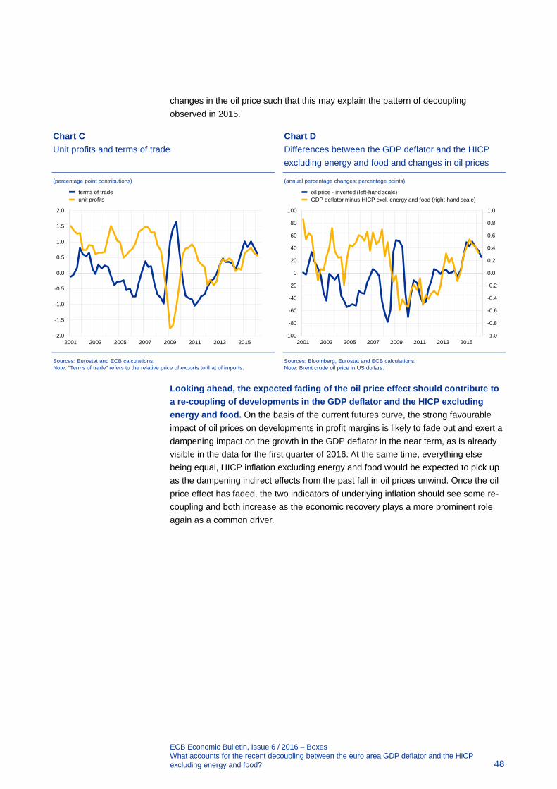
ECB Economic Bulletin, Issue 6 / 2016 – Boxes What accounts for the recent decoupling between the euro area GDP deflator and the HICP excluding energy and food? 48
changes in the oil price such that this may explain the pattern of decoupling observed in 2015.
Chart D Differences between the GDP deflator and the HICP excluding energy and food and changes in oil prices
(annual percentage changes; percentage points)
Sources: Bloomberg, Eurostat and ECB calculations. Note: Brent crude oil price in US dollars.
Looking ahead, the expected fading of the oil price effect should contribute to a re-coupling of developments in the GDP deflator and the HICP excluding energy and food. On the basis of the current futures curve, the strong favourable impact of oil prices on developments in profit margins is likely to fade out and exert a dampening impact on the growth in the GDP deflator in the near term, as is already visible in the data for the first quarter of 2016. At the same time, everything else being equal, HICP inflation excluding energy and food would be expected to pick up as the dampening indirect effects from the past fall in oil prices unwind. Once the oil price effect has faded, the two indicators of underlying inflation should see some re-coupling and both increase as the economic recovery plays a more prominent role again as a common driver.
-1.0
-0.8
-0.6
-0.4
-0.2
0.0
0.2
0.4
0.6
0.8
1.0
-100
-80
-60
-40
-20
0
20
40
60
80
100
2001 2003 2005 2007 2009 2011 2013 2015
oil price - inverted (left-hand scale)GDP deflator minus HICP excl. energy and food (right-hand scale)
Chart C Unit profits and terms of trade
(percentage point contributions)
Sources: Eurostat and ECB calculations. Note: “Terms of trade” refers to the relative price of exports to that of imports.
-2.0
-1.5
-1.0
-0.5
0.0
0.5
1.0
1.5
2.0
2001 2003 2005 2007 2009 2011 2013 2015
terms of tradeunit profits

ECB Economic Bulletin, Issue 6 / 2016 – Boxes Factors behind developments in average hours worked per person employed since 2008 49
6 Factors behind developments in average hours worked per person employed since 2008
Over the course of the euro area recovery, average hours worked per person employed have remained broadly unchanged, after falling significantly during the crisis. The total amount of labour input used by firms decreased considerably between the first quarter of 2008 and the second quarter of 2013, and the decline was more significant in terms of total hours worked than in terms of headcount employment. Underlying these developments was a decrease in average hours worked per person, which then remained flat during the recovery (see Chart A). Although the decline in average hours worked observed since the start of the crisis has generally been considered a cyclical phenomenon, after 12 quarters of increasing activity average hours worked per worker have shown no sign of a cyclical recovery. This box examines the underlying causes of this phenomenon and finds that the increase in part-time work plays a significant role.
Chart B Different measures of average hours worked per person
(index: 2008=100; annual data)
Sources: Eurostat and ECB calculations. Notes: In the EU labour force survey, the number of hours usually worked refers to the hours which a person normally works per week. The number of hours actually worked covers all hours including extra hours, regardless of whether or not they were paid, that a person worked during the reference week.
Hours worked were already following a downward trend even before the crisis. For the euro area, average hours worked calculated on the basis of national accounts as well as those reported in labour force surveys have declined significantly over the last two decades (see Chart B). Historical data suggest that hours worked have been declining for a much longer period.27 The decline in
27 See, for example, Lee, S., McCann, D. and Messenger, J.C., Working Time Around the World. Trends
in working hours, laws and policies in a global comparative perspective, International Labour Organisation, 2007 and Boppart, T. and Krusell, P., How much we work: The past, the present, and the future, 2016.
96
97
98
99
100
101
102
103
104
105
1995 1997 1999 2001 2003 2005 2007 2009 2011 2013 2015
national accounts, average hours workedlabour force survey, hours actually workedlabour force survey, hours usually worked
Chart A Euro area employment, total hours worked and average hours worked per person
(index: Q1 2008=100; quarterly data; working day and seasonally adjusted)
Sources: Eurostat and ECB calculations.
92
93
94
95
96
97
98
99
100
101
2008 2009 2010 2011 2012 2013 2014 2015 2016
average hours workedemploymenttotal hours worked
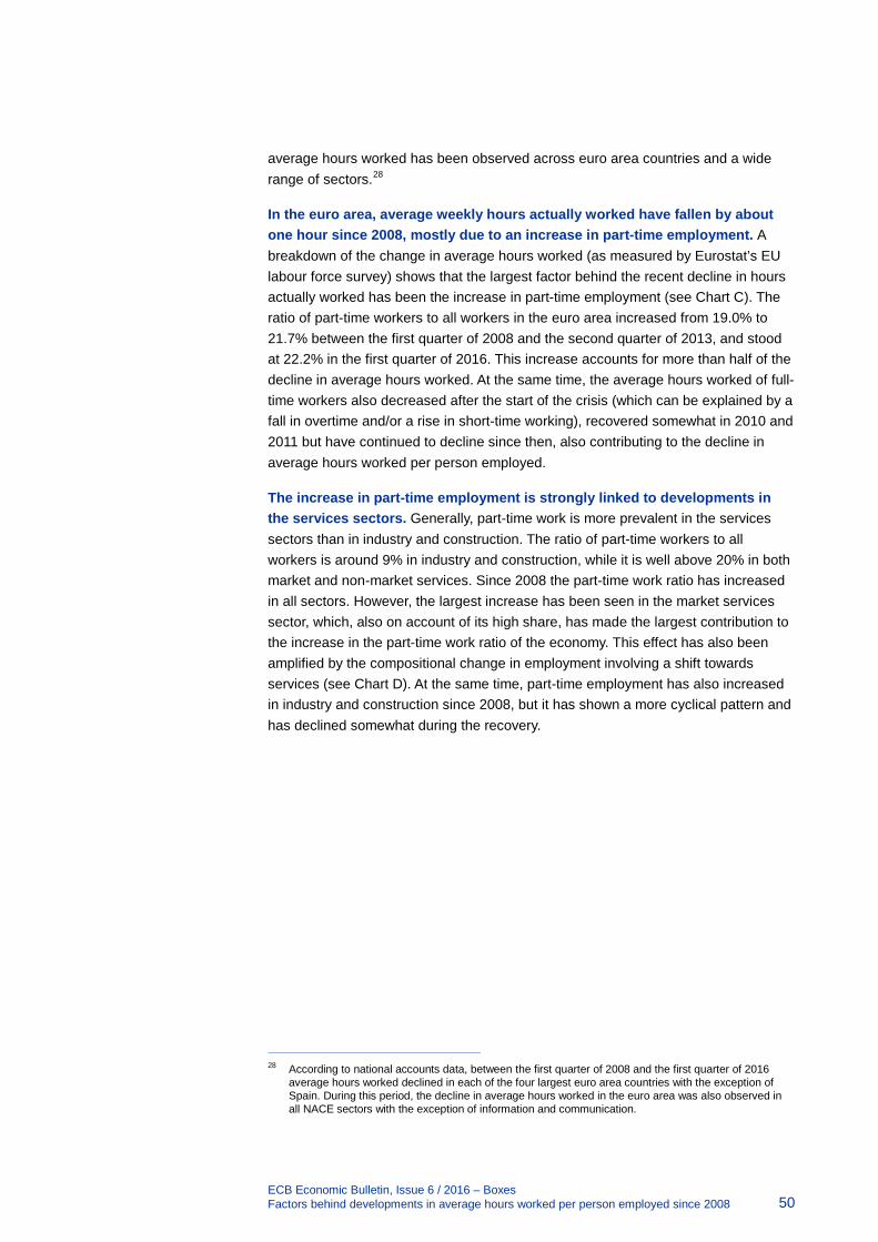
ECB Economic Bulletin, Issue 6 / 2016 – Boxes Factors behind developments in average hours worked per person employed since 2008 50
average hours worked has been observed across euro area countries and a wide range of sectors.28
In the euro area, average weekly hours actually worked have fallen by about one hour since 2008, mostly due to an increase in part-time employment. A breakdown of the change in average hours worked (as measured by Eurostat’s EU labour force survey) shows that the largest factor behind the recent decline in hours actually worked has been the increase in part-time employment (see Chart C). The ratio of part-time workers to all workers in the euro area increased from 19.0% to 21.7% between the first quarter of 2008 and the second quarter of 2013, and stood at 22.2% in the first quarter of 2016. This increase accounts for more than half of the decline in average hours worked. At the same time, the average hours worked of full-time workers also decreased after the start of the crisis (which can be explained by a fall in overtime and/or a rise in short-time working), recovered somewhat in 2010 and 2011 but have continued to decline since then, also contributing to the decline in average hours worked per person employed.
The increase in part-time employment is strongly linked to developments in the services sectors. Generally, part-time work is more prevalent in the services sectors than in industry and construction. The ratio of part-time workers to all workers is around 9% in industry and construction, while it is well above 20% in both market and non-market services. Since 2008 the part-time work ratio has increased in all sectors. However, the largest increase has been seen in the market services sector, which, also on account of its high share, has made the largest contribution to the increase in the part-time work ratio of the economy. This effect has also been amplified by the compositional change in employment involving a shift towards services (see Chart D). At the same time, part-time employment has also increased in industry and construction since 2008, but it has shown a more cyclical pattern and has declined somewhat during the recovery.
28 According to national accounts data, between the first quarter of 2008 and the first quarter of 2016
average hours worked declined in each of the four largest euro area countries with the exception of Spain. During this period, the decline in average hours worked in the euro area was also observed in all NACE sectors with the exception of information and communication.
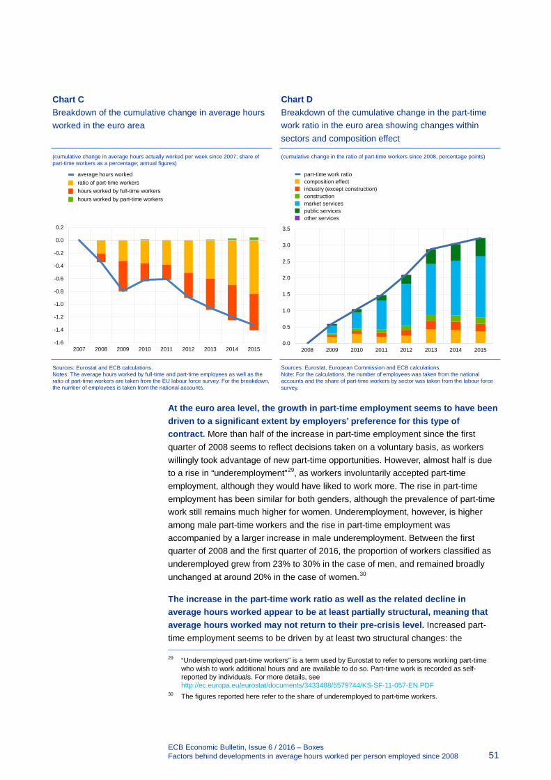
ECB Economic Bulletin, Issue 6 / 2016 – Boxes Factors behind developments in average hours worked per person employed since 2008 51
Chart D Breakdown of the cumulative change in the part-time work ratio in the euro area showing changes within sectors and composition effect
(cumulative change in the ratio of part-time workers since 2008, percentage points)
Sources: Eurostat, European Commission and ECB calculations. Note: For the calculations, the number of employees was taken from the national accounts and the share of part-time workers by sector was taken from the labour force survey.
At the euro area level, the growth in part-time employment seems to have been driven to a significant extent by employers’ preference for this type of contract. More than half of the increase in part-time employment since the first quarter of 2008 seems to reflect decisions taken on a voluntary basis, as workers willingly took advantage of new part-time opportunities. However, almost half is due to a rise in “underemployment”29, as workers involuntarily accepted part-time employment, although they would have liked to work more. The rise in part-time employment has been similar for both genders, although the prevalence of part-time work still remains much higher for women. Underemployment, however, is higher among male part-time workers and the rise in part-time employment was accompanied by a larger increase in male underemployment. Between the first quarter of 2008 and the first quarter of 2016, the proportion of workers classified as underemployed grew from 23% to 30% in the case of men, and remained broadly unchanged at around 20% in the case of women.30
The increase in the part-time work ratio as well as the related decline in average hours worked appear to be at least partially structural, meaning that average hours worked may not return to their pre-crisis level. Increased part-time employment seems to be driven by at least two structural changes: the 29 “Underemployed part-time workers” is a term used by Eurostat to refer to persons working part-time
who wish to work additional hours and are available to do so. Part-time work is recorded as self-reported by individuals. For more details, see http://ec.europa.eu/eurostat/documents/3433488/5579744/KS-SF-11-057-EN.PDF
30 The figures reported here refer to the share of underemployed to part-time workers.
0.0
0.5
1.0
1.5
2.0
2.5
3.0
3.5
2008 2009 2010 2011 2012 2013 2014 2015
part-time work ratiocomposition effectindustry (except construction) constructionmarket servicespublic servicesother services
Chart C Breakdown of the cumulative change in average hours worked in the euro area
(cumulative change in average hours actually worked per week since 2007; share of part-time workers as a percentage; annual figures)
Sources: Eurostat and ECB calculations. Notes: The average hours worked by full-time and part-time employees as well as the ratio of part-time workers are taken from the EU labour force survey. For the breakdown, the number of employees is taken from the national accounts.
-1.6
-1.4
-1.2
-1.0
-0.8
-0.6
-0.4
-0.2
0.0
0.2
2007 2008 2009 2010 2011 2012 2013 2014 2015
average hours worked ratio of part-time workershours worked by full-time workers hours worked by part-time workers

ECB Economic Bulletin, Issue 6 / 2016 – Boxes Factors behind developments in average hours worked per person employed since 2008 52
increasing share of market services and the resulting higher demand for part-time work, and the increased part-time labour supply (owing to, among other things, the increasing participation of women and those above 55). Unless there is a reversal of the long-term trend towards higher employment in services, the part-time employment ratio is likely to continue to increase and average hours worked to remain lower than the levels seen before the crisis.

ECB Economic Bulletin, Issue 6 / 2016 – Article The employment-GDP relationship since the crisis 53
Article
1 The employment-GDP relationship since the crisis
The continued employment growth seen across the euro area since the onset of the recovery in 2013 has been stronger than expected. Differences in the responsiveness of employment growth to GDP growth between the pre- and post-crisis periods suggest a possible structural change in the underlying employment-GDP relationship. This article explores the factors driving the employment-GDP relationship. It suggests that the changing sectoral composition of GDP growth towards a larger services sector, a shift in the composition of employment towards part-time employment, and structural labour market reforms and fiscal measures in some countries underlie some strengthening in the underlying employment-GDP relationship since the start of the recovery.
The relationship between euro area employment and GDP
The recovery in euro area GDP since the second quarter of 2013 has been accompanied by higher than expected employment growth. This article assesses the extent to which the stronger than expected employment growth seen over the recovery is likely to persist and examines some of the factors likely to be contributing to this. From a central bank perspective, this topic is important because the labour market recovery is crucial for the strength of confidence and consumption in the aftermath of the crisis. While the earlier weakening of the relationship between GDP growth and the unemployment rate (Okun’s law), or between GDP and employment growth, has been documented and explained in the literature31, much less attention has, so far, been paid to the strong “reconnection” between employment and GDP growth over the recovery.
To some extent, it is surprising that the employment-GDP relationship over the recovery has been as strong as in the pre-crisis years. Before the onset of the Great Recession in 2008, euro area employment growth co-moved closely with GDP. In retrospect, however, the strong employment growth experienced in some countries in the pre-crisis period had been associated with the emergence of sectoral imbalances, which were later viewed as unsustainable in the longer term. Nevertheless, since the onset of the euro area recovery in GDP, employment responses to GDP growth have been at least as strong as in the pre-crisis period.
Both cyclical and structural changes are likely to have contributed to the higher than expected responsiveness of euro area employment to GDP since the rebound. The cyclical reasons include strong rebounds following large 31 See, for example, Klinger, S. and Weber, E., “On GDP-Employment Decoupling in Germany”, Institute
for Employment Research, IAB-Discussion Paper, 21/2014, and Burggraeve, K., de Walque, G. and Zimmer, H., “The relationship between economic growth and employment”, National Bank of Belgium Economic Review, June 2015.
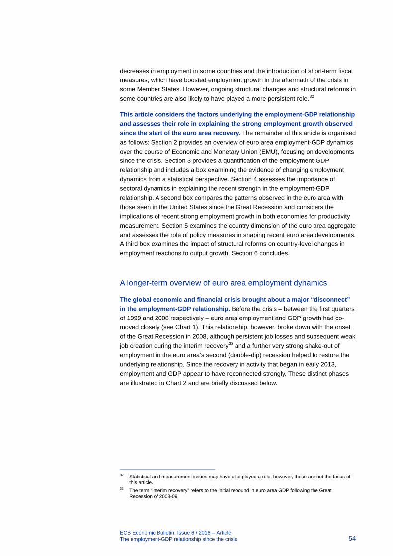
ECB Economic Bulletin, Issue 6 / 2016 – Article The employment-GDP relationship since the crisis 54
decreases in employment in some countries and the introduction of short-term fiscal measures, which have boosted employment growth in the aftermath of the crisis in some Member States. However, ongoing structural changes and structural reforms in some countries are also likely to have played a more persistent role.32
This article considers the factors underlying the employment-GDP relationship and assesses their role in explaining the strong employment growth observed since the start of the euro area recovery. The remainder of this article is organised as follows: Section 2 provides an overview of euro area employment-GDP dynamics over the course of Economic and Monetary Union (EMU), focusing on developments since the crisis. Section 3 provides a quantification of the employment-GDP relationship and includes a box examining the evidence of changing employment dynamics from a statistical perspective. Section 4 assesses the importance of sectoral dynamics in explaining the recent strength in the employment-GDP relationship. A second box compares the patterns observed in the euro area with those seen in the United States since the Great Recession and considers the implications of recent strong employment growth in both economies for productivity measurement. Section 5 examines the country dimension of the euro area aggregate and assesses the role of policy measures in shaping recent euro area developments. A third box examines the impact of structural reforms on country-level changes in employment reactions to output growth. Section 6 concludes.
A longer-term overview of euro area employment dynamics
The global economic and financial crisis brought about a major “disconnect” in the employment-GDP relationship. Before the crisis – between the first quarters of 1999 and 2008 respectively – euro area employment and GDP growth had co-moved closely (see Chart 1). This relationship, however, broke down with the onset of the Great Recession in 2008, although persistent job losses and subsequent weak job creation during the interim recovery33 and a further very strong shake-out of employment in the euro area’s second (double-dip) recession helped to restore the underlying relationship. Since the recovery in activity that began in early 2013, employment and GDP appear to have reconnected strongly. These distinct phases are illustrated in Chart 2 and are briefly discussed below.
32 Statistical and measurement issues may have also played a role; however, these are not the focus of
this article. 33 The term “interim recovery” refers to the initial rebound in euro area GDP following the Great
Recession of 2008-09.

ECB Economic Bulletin, Issue 6 / 2016 – Article The employment-GDP relationship since the crisis 55
When the global Great Recession hit the euro area economy in 2008, euro area employment initially contracted relatively moderately, given the sharp decline in GDP growth, but this was to some extent countered over the course of the interim rebound. While euro area employment initially contracted only modestly in the first quarters of the Great Recession, the employment decline continued for several quarters into the interim rebound in activity, which lasted from the third quarter of 2009 until the third quarter of 2011 (as shown by the yellow line in Chart 2). Moreover, despite a marked recovery in euro area GDP over the subsequent interim rebound, euro area employment barely rose, in part reflecting the delayed effects of earlier labour hoarding (see the red line in Chart 2). The marked disconnect in the relationship between employment and GDP has been widely reported and analysed in the literature.34
Chart 2 Cumulative changes in euro area GDP and employment since the start of the crisis
(cumulative changes; percentages; thousands)
Sources: Eurostat and ECB calculations.
Since the start of the second euro area recession and over the subsequent recovery, the euro area employment-GDP relationship appears to have “reconnected”. As the euro area slid back into recession (from the fourth quarter of 2011), employment developments followed the decline in GDP closely (as shown by the green line in Chart 2). Thereafter, with the rebound in activity (from the second quarter of 2013), employment also quickly returned to positive growth – within one
34 See, for instance, Euro area labour markets and the crisis, Structural Issues Report, ECB, October
2012, and the updated version, published as “Comparisons and contrasts of the impact of the crisis on euro area labour markets”, Occasional Paper Series, No 159, ECB, February 2015.
-6,000
-4,000
-2,000
0
2,000
4,000
6,000
-6
-4
-2
0
2
4
6
Q12008
Q12009
Q12010
Q12011
Q12012
Q12013
Q12014
Q12015
Q12016
losses/rebounds of euro area GDP (left-hand scale)change in employment following onset of Great Recession (right-hand scale)change in employment following onset of interim rebound (right-hand scale)change in employment following onset of double dip (right-hand scale)change in employment following onset of recovery (right-hand scale)
Chart 1 Growth rates of real GDP and employment in the euro area since 1999
(quarter-on-quarter growth rates)
Sources: Eurostat and ECB calculations.
-3.5
-3.0
-2.5
-2.0
-1.5
-1.0
-0.5
0.0
0.5
1.0
1.5
1999 2001 2003 2005 2007 2009 2011 2013 2015
real GDPemployment

ECB Economic Bulletin, Issue 6 / 2016 – Article The employment-GDP relationship since the crisis 56
quarter of the GDP rebound – and has since expanded strongly in line with GDP dynamics (see the light blue line in Chart 2).
Despite the strengthening of the employment-GDP relationship of late, euro area employment remains slightly below pre-crisis levels. As Chart 3 shows, in the first quarter of 201635 euro area employment was still around 1% below the pre-crisis peak seen in the first quarter of 2008. However, the slight shortfall in headcount employment contrasts markedly with developments in total hours worked. In the first five years of the crisis, developments in headcount employment and total hours worked diverged substantially, with the latter remaining considerably below pre-crisis levels, following a further significant reduction in total hours worked over the course of the second euro area recession. Following this strong decline, it had been expected that subsequent increases in activity would be met by increases in working hours of existing headcount (resulting in increases in measured average working hours per person employed).36 In practice, however, average
hours worked per person employed have barely changed since 2013. Instead, the evolution of total hours worked has merely reflected the expansion in employment (see also the box entitled “Factors behind developments in average hours worked per person employed since 2008” in this issue of the Economic Bulletin).
Over the recovery, employment forecasts for the euro area have been continually revised upwards by a wide range of forecasters. It seems that forecasters had also anticipated that firms would expand the working hours of their incumbent employees, rather than expand headcount. Chart 4 shows that Eurosystem and ECB staff projections consistently underestimated euro area employment growth over the 2013-15 interval, even as the recovery was under way. Similar errors are evident in the forecasts for the euro area from other institutions, such as the European Commission, the IMF and the OECD, as forecasters there also were caught out by a stronger than expected employment response to GDP growth, rather than forecast errors for GDP. 37
35 This article is based on data available up to the end of June 2016. 36 For example, the European Commission held the view that “the current low level of average hours
worked does not represent necessarily a new normal, as it is accompanied by a significant increase in involuntary part-time employment, which has a clear cyclical pattern and can be expected to be reabsorbed during the recovery”. Labour Market and Wage Developments in Europe 2015, European Commission, 2015, p.24.
37 Indeed, GDP growth was lower than projected in 2014 and – at the time – similar to the projections in 2015, while employment growth was higher than anticipated in both years. The recent substantial revisions to Irish GDP were not taken into consideration in this assessment.
Chart 3 Evolution of real GDP, employment and total hours worked since the start of the crisis
(index: 2008 = 100)
Sources: Eurostat and ECB calculations.
92
93
94
95
96
97
98
99
100
101
Q12008
Q12009
Q12010
Q12011
Q12012
Q12013
Q12014
Q12015
Q12016
employmenttotal hours workedreal GDP
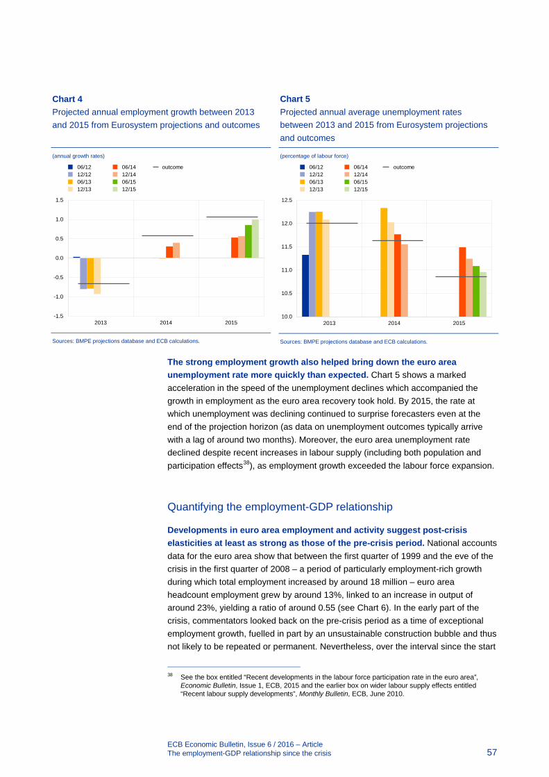
ECB Economic Bulletin, Issue 6 / 2016 – Article The employment-GDP relationship since the crisis 57
Chart 5 Projected annual average unemployment rates between 2013 and 2015 from Eurosystem projections and outcomes
(percentage of labour force)
Sources: BMPE projections database and ECB calculations.
The strong employment growth also helped bring down the euro area unemployment rate more quickly than expected. Chart 5 shows a marked acceleration in the speed of the unemployment declines which accompanied the growth in employment as the euro area recovery took hold. By 2015, the rate at which unemployment was declining continued to surprise forecasters even at the end of the projection horizon (as data on unemployment outcomes typically arrive with a lag of around two months). Moreover, the euro area unemployment rate declined despite recent increases in labour supply (including both population and participation effects38), as employment growth exceeded the labour force expansion.
Quantifying the employment-GDP relationship
Developments in euro area employment and activity suggest post-crisis elasticities at least as strong as those of the pre-crisis period. National accounts data for the euro area show that between the first quarter of 1999 and the eve of the crisis in the first quarter of 2008 – a period of particularly employment-rich growth during which total employment increased by around 18 million – euro area headcount employment grew by around 13%, linked to an increase in output of around 23%, yielding a ratio of around 0.55 (see Chart 6). In the early part of the crisis, commentators looked back on the pre-crisis period as a time of exceptional employment growth, fuelled in part by an unsustainable construction bubble and thus not likely to be repeated or permanent. Nevertheless, over the interval since the start
38 See the box entitled “Recent developments in the labour force participation rate in the euro area”,
Economic Bulletin, Issue 1, ECB, 2015 and the earlier box on wider labour supply effects entitled “Recent labour supply developments”, Monthly Bulletin, ECB, June 2010.
10.0
10.5
11.0
11.5
12.0
12.5
2013 2014 2015
06/1212/1206/1312/13
06/1412/1406/1512/15
outcome
Chart 4 Projected annual employment growth between 2013 and 2015 from Eurosystem projections and outcomes
(annual growth rates)
Sources: BMPE projections database and ECB calculations.
-1.5
-1.0
-0.5
0.0
0.5
1.0
1.5
2013 2014 2015
06/1212/1206/1312/13
06/1412/1406/1512/15
outcome
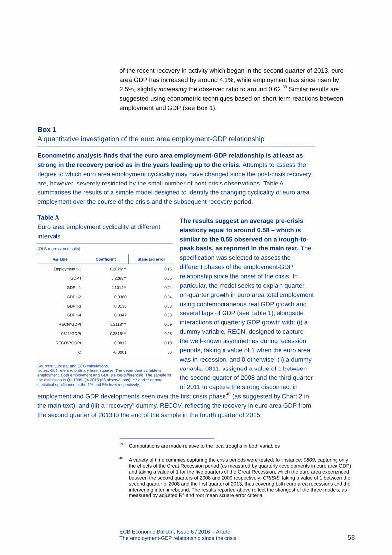
ECB Economic Bulletin, Issue 6 / 2016 – Article The employment-GDP relationship since the crisis 58
of the recent recovery in activity which began in the second quarter of 2013, euro area GDP has increased by around 4.1%, while employment has since risen by 2.5%, slightly increasing the observed ratio to around 0.62.39 Similar results are suggested using econometric techniques based on short-term reactions between employment and GDP (see Box 1).
Box 1 A quantitative investigation of the euro area employment-GDP relationship
Econometric analysis finds that the euro area employment-GDP relationship is at least as strong in the recovery period as in the years leading up to the crisis. Attempts to assess the degree to which euro area employment cyclicality may have changed since the post-crisis recovery are, however, severely restricted by the small number of post-crisis observations. Table A summarises the results of a simple model designed to identify the changing cyclicality of euro area employment over the course of the crisis and the subsequent recovery period.
The results suggest an average pre-crisis elasticity equal to around 0.58 – which is similar to the 0.55 observed on a trough-to-peak basis, as reported in the main text. The specification was selected to assess the different phases of the employment-GDP relationship since the onset of the crisis. In particular, the model seeks to explain quarter-on-quarter growth in euro area total employment using contemporaneous real GDP growth and several lags of GDP (see Table 1), alongside interactions of quarterly GDP growth with: (i) a dummy variable, RECN, designed to capture the well-known asymmetries during recession periods, taking a value of 1 when the euro area was in recession, and 0 otherwise; (ii) a dummy variable, 0811, assigned a value of 1 between the second quarter of 2008 and the third quarter of 2011 to capture the strong disconnect in
employment and GDP developments seen over the first crisis phase40 (as suggested by Chart 2 in the main text); and (iii) a “recovery” dummy, RECOV, reflecting the recovery in euro area GDP from the second quarter of 2013 to the end of the sample in the fourth quarter of 2015.
39 Computations are made relative to the local troughs in both variables.
40 A variety of time dummies capturing the crisis periods were tested, for instance: 0809, capturing only the effects of the Great Recession period (as measured by quarterly developments in euro area GDP) and taking a value of 1 for the five quarters of the Great Recession, which the euro area experienced between the second quarters of 2008 and 2009 respectively; CRISIS, taking a value of 1 between the second quarter of 2008 and the first quarter of 2013, thus covering both euro area recessions and the intervening interim rebound. The results reported above reflect the strongest of the three models, as measured by adjusted R2 and root mean square error criteria.
Table A Euro area employment cyclicality at different intervals
(OLS regression results)
Variable Coefficient Standard error
Employment t-1 0.2826*** 0.15
GDP t 0.2283** 0.05
GDP t-1 0.1014** 0.04
GDP t-2 0.0380 0.04
GDP t-3 0.0135 0.03
GDP t-4 0.0347 0.03
RECN*GDPt 0.2118*** 0.09
0811*GDPt -0.2818*** 0.08
RECOV*GDPt 0.0812 0.10
C -0.0001 00
Sources: Eurostat and ECB calculations. Notes: OLS refers to ordinary least squares. The dependent variable is employment. Both employment and GDP are log-differenced. The sample for the estimation is Q1 1999-Q4 2015 (68 observations). *** and ** denote statistical significance at the 1% and 5% level respectively.

ECB Economic Bulletin, Issue 6 / 2016 – Article The employment-GDP relationship since the crisis 59
Moreover, the results show a marked and statistically significant disconnect in the longer-term employment-GDP relationship following the start of the Great Recession. Recession asymmetries were generally found to be strongly positive and significant (see the strong positive coefficient on the interaction term, RECN*GDPt). This suggests that euro area employment typically falls at an accelerated rate during recessions, rather than at the same rate at which it grows during periods of GDP expansion. However, the model finds a strong reduction in the employment-GDP relationship over the period of disconnect following the onset of the Great Recession (see the strong negative coefficient on the interaction term 0811), reflecting a marked moderation in employment losses (as a consequence of well-documented labour hoarding in some euro area countries41) over this period – and to an extent large enough to fully offset typical recession asymmetries.
In the recovery phase, the term aiming to capture any increase in euro area employment cyclicality in the aftermath of
the crisis is positive, but statistically insignificant. Leaving aside the significance issues, which may be attributable in part to the low number of observations since the recovery, the implied euro area employment elasticity rises from around 0.58 pre-crisis to almost 0.70 with the inclusion of a post-crisis interaction dummy, RECOV.42 Clearly, it is too early to be certain whether the stronger increase in employment growth seen over the recovery reflects merely an ongoing cyclical response to the previous strong decline in euro area employment seen over the crisis or the emergence of a stronger employment-GDP relationship. Nevertheless, over the Q2 2013-Q4 2015 period, the inclusion of the recovery term markedly improves forecasts of euro area employment, compared either with forecasts based solely on pre-crisis relationships or those which simply take account of recession asymmetries and the Great Recession disconnect (see Chart A). Given the wide-reaching changes under way in many euro area countries – including in the sectoral composition of output and employment, as well as to labour market institutions as a consequence of structural reforms – further careful monitoring of the employment-GDP relationship as the recovery unfolds seems warranted.
41 See, for example, the article entitled “The impact of the economic crisis on euro area labour markets” in
the October 2014 issue of the ECB Monthly Bulletin. 42 Long-term implied elasticities are reported (i.e correcting for the impact of the lagged dependent
variable).
Chart A Estimated euro area rebound in employment since the crisis compared with actual developments
(employment levels; thousands)
Sources: Eurostat and ECB calculations. Notes: Comparison of actual employment outcomes (green line) with forecasts for the period from Q2 2013 to Q4 2015 based on: (i) the pre-crisis relationship only (blue line); (ii) interaction terms for recession asymmetries (RECN) and the Great Recession disconnect (0811), shown by the yellow line; and (iii) interaction terms for recession asymmetries (RECN), the Great Recession disconnect (0811) and the recovery dummy (RECOV), as illustrated by the red line.
148,000
149,000
150,000
151,000
152,000
153,000
154,000
155,000
Q12008
Q12009
Q12010
Q12011
Q12012
Q12013
Q12014
Q12015
pre-crisis model onlymodel with recession dummy andGreat Recession disconnectfull modelemployment outcome
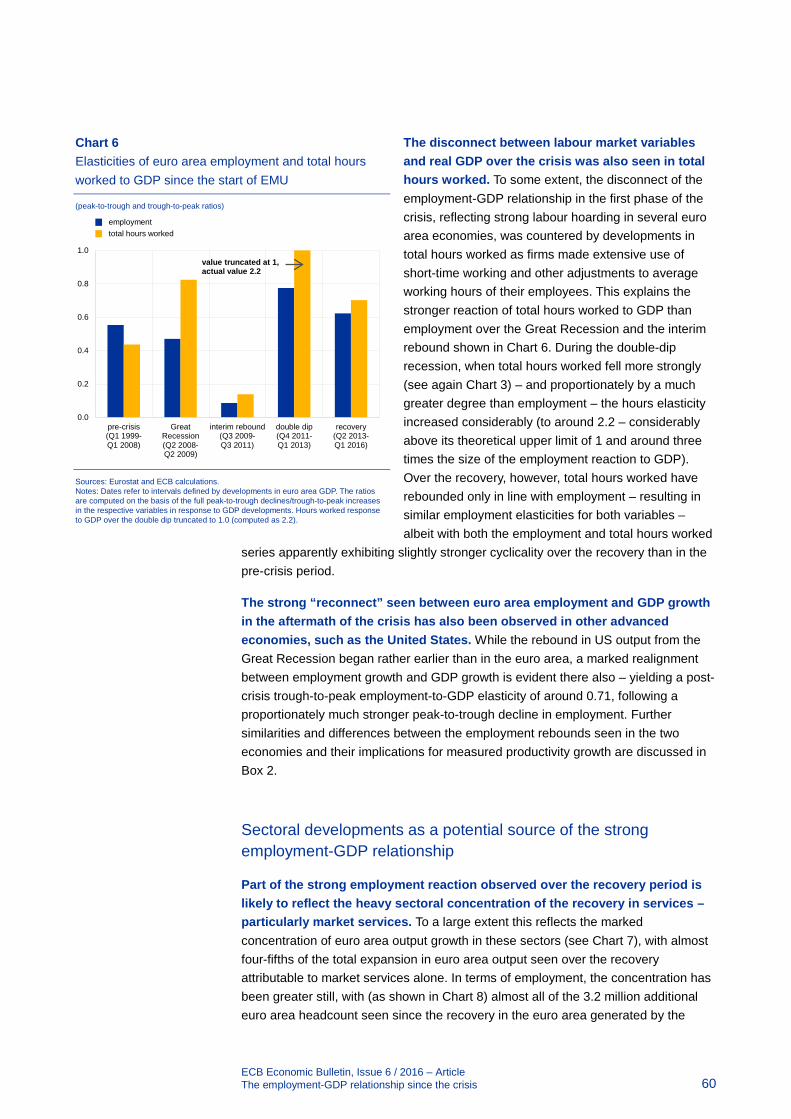
ECB Economic Bulletin, Issue 6 / 2016 – Article The employment-GDP relationship since the crisis 60
The disconnect between labour market variables and real GDP over the crisis was also seen in total hours worked. To some extent, the disconnect of the employment-GDP relationship in the first phase of the crisis, reflecting strong labour hoarding in several euro area economies, was countered by developments in total hours worked as firms made extensive use of short-time working and other adjustments to average working hours of their employees. This explains the stronger reaction of total hours worked to GDP than employment over the Great Recession and the interim rebound shown in Chart 6. During the double-dip recession, when total hours worked fell more strongly (see again Chart 3) – and proportionately by a much greater degree than employment – the hours elasticity increased considerably (to around 2.2 – considerably above its theoretical upper limit of 1 and around three times the size of the employment reaction to GDP). Over the recovery, however, total hours worked have rebounded only in line with employment – resulting in similar employment elasticities for both variables – albeit with both the employment and total hours worked
series apparently exhibiting slightly stronger cyclicality over the recovery than in the pre-crisis period.
The strong “reconnect” seen between euro area employment and GDP growth in the aftermath of the crisis has also been observed in other advanced economies, such as the United States. While the rebound in US output from the Great Recession began rather earlier than in the euro area, a marked realignment between employment growth and GDP growth is evident there also – yielding a post-crisis trough-to-peak employment-to-GDP elasticity of around 0.71, following a proportionately much stronger peak-to-trough decline in employment. Further similarities and differences between the employment rebounds seen in the two economies and their implications for measured productivity growth are discussed in Box 2.
Sectoral developments as a potential source of the strong employment-GDP relationship
Part of the strong employment reaction observed over the recovery period is likely to reflect the heavy sectoral concentration of the recovery in services – particularly market services. To a large extent this reflects the marked concentration of euro area output growth in these sectors (see Chart 7), with almost four-fifths of the total expansion in euro area output seen over the recovery attributable to market services alone. In terms of employment, the concentration has been greater still, with (as shown in Chart 8) almost all of the 3.2 million additional euro area headcount seen since the recovery in the euro area generated by the
Chart 6 Elasticities of euro area employment and total hours worked to GDP since the start of EMU
(peak-to-trough and trough-to-peak ratios)
Sources: Eurostat and ECB calculations. Notes: Dates refer to intervals defined by developments in euro area GDP. The ratios are computed on the basis of the full peak-to-trough declines/trough-to-peak increases in the respective variables in response to GDP developments. Hours worked response to GDP over the double dip truncated to 1.0 (computed as 2.2).
0.0
0.2
0.4
0.6
0.8
1.0
pre-crisis(Q1 1999-Q1 2008)
GreatRecession(Q2 2008-Q2 2009)
interim rebound(Q3 2009-Q3 2011)
double dip(Q4 2011-Q1 2013)
recovery(Q2 2013-Q1 2016)
value truncated at 1, actual value 2.2
employmenttotal hours worked
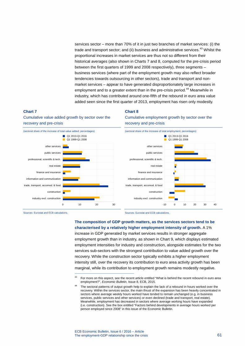
ECB Economic Bulletin, Issue 6 / 2016 – Article The employment-GDP relationship since the crisis 61
services sector – more than 70% of it in just two branches of market services: (i) the trade and transport sector; and (ii) business and administrative services.43 Whilst the proportional increases in market services are thus not so different from their historical averages (also shown in Charts 7 and 8, computed for the pre-crisis period between the first quarters of 1999 and 2008 respectively), three segments – business services (where part of the employment growth may also reflect broader tendencies towards outsourcing in other sectors), trade and transport and non-market services – appear to have generated disproportionately large increases in employment and to a greater extent than in the pre-crisis period.44 Meanwhile in industry, which has contributed around one-fifth of the rebound in euro area value added seen since the first quarter of 2013, employment has risen only modestly.
Chart 8 Cumulative employment growth by sector over the recovery and pre-crisis
(sectoral share of the increase of total employment; percentages)
Sources: Eurostat and ECB calculations.
The composition of GDP growth matters, as the services sectors tend to be characterised by a relatively higher employment intensity of growth. A 1% increase in GDP generated by market services results in stronger aggregate employment growth than in industry, as shown in Chart 9, which displays estimated employment intensities for industry and construction, alongside estimates for the two services sub-sectors with the strongest contribution to value added growth over the recovery. While the construction sector typically exhibits a higher employment intensity still, over the recovery its contribution to euro area activity growth has been marginal, while its contribution to employment growth remains modestly negative. 43 For more on this aspect, see the recent article entitled “What is behind the recent rebound in euro area
employment?”, Economic Bulletin, Issue 8, ECB, 2015. 44 The sectoral patterns of output growth help to explain the lack of a rebound in hours worked over the
recovery. Within the services sector, the main thrust of the expansion has been heavily concentrated in sectors where average weekly hours worked have tended to remain unchanged (e.g. in business services, public services and other services) or even declined (trade and transport, real estate). Meanwhile, employment has decreased in sectors where average working hours have expanded (i.e. construction). See the box entitled “Factors behind developments in average hours worked per person employed since 2008” in this issue of the Economic Bulletin.
-10 0 10 20 30 40
industry excl. construction
construction
trade, transport, accomod. & food
information and communication
finance and insurance
real estate
professional, scientific & tech.
public services
other services
Q1 2013-Q1 2016Q1 1999-Q1 2008
Chart 7 Cumulative value added growth by sector over the recovery and pre-crisis
(sectoral share of the increase of total value added; percentages)
Sources: Eurostat and ECB calculations.
0 10 20 30
industry excl. construction
construction
trade, transport, accomod. & food
information and communication
finance and insurance
real estate
professional, scientific & tech.
public services
other services
Q1 2013-Q1 2016Q1 1999-Q1 2008
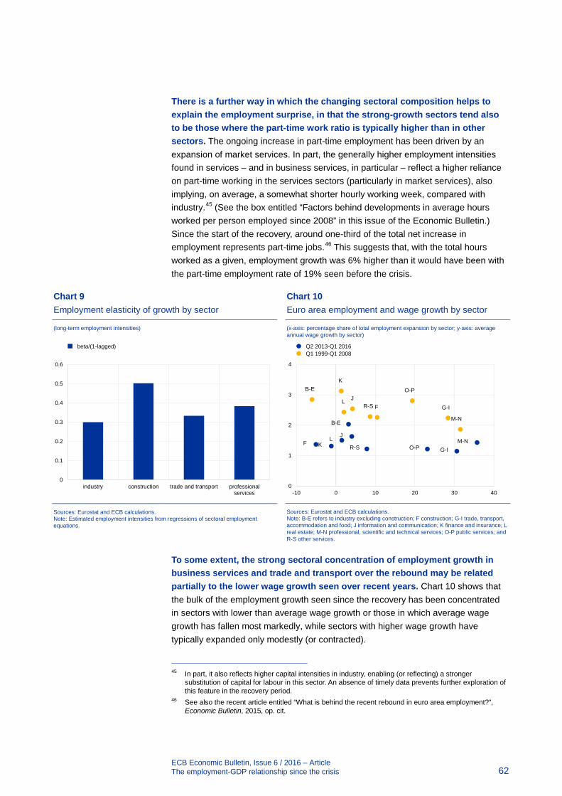
ECB Economic Bulletin, Issue 6 / 2016 – Article The employment-GDP relationship since the crisis 62
There is a further way in which the changing sectoral composition helps to explain the employment surprise, in that the strong-growth sectors tend also to be those where the part-time work ratio is typically higher than in other sectors. The ongoing increase in part-time employment has been driven by an expansion of market services. In part, the generally higher employment intensities found in services – and in business services, in particular – reflect a higher reliance on part-time working in the services sectors (particularly in market services), also implying, on average, a somewhat shorter hourly working week, compared with industry.45 (See the box entitled “Factors behind developments in average hours worked per person employed since 2008” in this issue of the Economic Bulletin.) Since the start of the recovery, around one-third of the total net increase in employment represents part-time jobs.46 This suggests that, with the total hours worked as a given, employment growth was 6% higher than it would have been with the part-time employment rate of 19% seen before the crisis.
Chart 10 Euro area employment and wage growth by sector
(x-axis: percentage share of total employment expansion by sector; y-axis: average annual wage growth by sector)
Sources: Eurostat and ECB calculations. Note: B-E refers to industry excluding construction; F construction; G-I trade, transport, accommodation and food; J information and communication; K finance and insurance; L real estate; M-N professional, scientific and technical services; O-P public services; and R-S other services.
To some extent, the strong sectoral concentration of employment growth in business services and trade and transport over the rebound may be related partially to the lower wage growth seen over recent years. Chart 10 shows that the bulk of the employment growth seen since the recovery has been concentrated in sectors with lower than average wage growth or those in which average wage growth has fallen most markedly, while sectors with higher wage growth have typically expanded only modestly (or contracted).
45 In part, it also reflects higher capital intensities in industry, enabling (or reflecting) a stronger
substitution of capital for labour in this sector. An absence of timely data prevents further exploration of this feature in the recovery period.
46 See also the recent article entitled “What is behind the recent rebound in euro area employment?”, Economic Bulletin, 2015, op. cit.
B-E
FG-I
J
KL M-N
O-PR-S
B-E
F G-IJ
K
L
M-N
O-P
R-S
0
1
2
3
4
-10 0 10 20 30 40
Q2 2013-Q1 2016Q1 1999-Q1 2008
Chart 9 Employment elasticity of growth by sector
(long-term employment intensities)
Sources: Eurostat and ECB calculations. Note: Estimated employment intensities from regressions of sectoral employment equations.
0
0.1
0.2
0.3
0.4
0.5
0.6
industry construction trade and transport professionalservices
beta/(1-lagged)
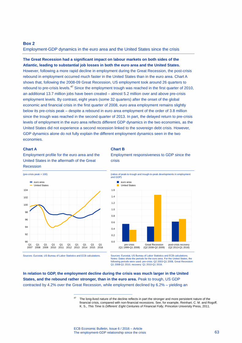
ECB Economic Bulletin, Issue 6 / 2016 – Article The employment-GDP relationship since the crisis 63
Box 2 Employment-GDP dynamics in the euro area and the United States since the crisis
The Great Recession had a significant impact on labour markets on both sides of the Atlantic, leading to substantial job losses in both the euro area and the United States. However, following a more rapid decline in employment during the Great Recession, the post-crisis rebound in employment occurred much faster in the United States than in the euro area. Chart A shows that, following the 2008-09 Great Recession, US employment took around 26 quarters to rebound to pre-crisis levels.47 Since the employment trough was reached in the first quarter of 2010, an additional 13.7 million jobs have been created – almost 5.2 million over and above pre-crisis employment levels. By contrast, eight years (some 32 quarters) after the onset of the global economic and financial crisis in the first quarter of 2008, euro area employment remains slightly below its pre-crisis peak – despite a rebound in euro area employment of the order of 3.8 million since the trough was reached in the second quarter of 2013. In part, the delayed return to pre-crisis levels of employment in the euro area reflects different GDP dynamics in the two economies, as the United States did not experience a second recession linked to the sovereign debt crisis. However, GDP dynamics alone do not fully explain the different employment dynamics seen in the two economies.
Chart B Employment responsiveness to GDP since the crisis
(ratios of peak-to-trough and trough-to-peak developments in employment and GDP)
Sources: Eurostat, US Bureau of Labor Statistics and ECB calculations. Notes: Dates show the periods for the euro area. For the United States, the following periods were used: pre-crisis: Q2 2003-Q1 2008, Great Recession: Q1 2008-Q1 2010, recovery: Q1 2010-Q1 2016.
In relation to GDP, the employment decline during the crisis was much larger in the United States, and the rebound rather stronger, than in the euro area. Peak to trough, US GDP contracted by 4.2% over the Great Recession, while employment declined by 6.2% – yielding an
47 The long-lived nature of the decline reflects in part the stronger and more persistent nature of the
financial crisis, compared with non-financial recessions. See, for example, Reinhart, C. M. and Rogoff, K. S., This Time Is Different: Eight Centuries of Financial Folly, Princeton University Press, 2011.
0.0
0.2
0.4
0.6
0.8
1.0
1.2
1.4
1.6
pre-crisis(Q1 1999-Q1 2008)
Great Recession(Q2 2008-Q2 2009)
post-crisis recovery(Q2 2013-Q1 2016)
euro areaUnited States
Chart A Employment profile for the euro area and the United States in the aftermath of the Great Recession
(pre-crisis peak = 100)
Sources: Eurostat, US Bureau of Labor Statistics and ECB calculations.
90
92
94
96
98
100
102
104
Q12007
Q12008
Q12009
Q12010
Q12011
Q12012
Q12013
Q12014
Q12015
Q12016
euro areaUnited States

ECB Economic Bulletin, Issue 6 / 2016 – Article The employment-GDP relationship since the crisis 64
“elasticity” of employment to GDP losses of around 1.45. While to some extent this is likely to reflect the greater labour market flexibility which typically characterises the US labour market – in part as a consequence of notably lower employment protection legislation there48 – the reaction was clearly stronger than in many earlier US recessions, when employment losses were generally proportionately smaller than output losses.49 Given the severity and duration of the recession, it is likely that US firms hoarded considerably less labour than usually seen across post-war recessions.50 Chart B shows the estimated elasticities of the employment response to GDP developments for the two economies over the crisis period and into the recovery. The US experience stands in marked contrast to the strong disconnect between employment and GDP developments that was evident in the euro area in the early phases of the crisis (see the section entitled “A longer-term overview of euro area employment dynamics” and Chart 2). As has been shown, following the onset of the Great Recession, euro area GDP fell by some 5.7%, while employment initially declined by 2.7% (peak-to-local trough, reached in the first quarter of 2010), yielding a ratio of around 0.47. Over this period, institutional support – in particular from widespread reliance on short-time working schemes and other job-saving measures in many euro area countries51 – helped cushion the impact of the strong GDP losses on euro area employment to a greater degree than in the United States.
The expansion in US employment relative to GDP has also been proportionately stronger in the upturn than in the euro area. Chart B demonstrates that following the respective troughs in GDP reached after the Great Recession, the employment response to GDP has been more muted in the euro area than in the United States, yielding an elasticity of around 0.62, compared with 0.71 in the United States. In advance of the crisis, it seems that the elasticity in the euro area had been somewhat stronger than in the United States, reflecting in part the protracted period of “jobless growth” following the bursting of the dot-com bubble in the early 2000s.
The rebound in employment in the United States has been somewhat more broadly spread across economic sectors than that in the euro area. In both regions, the business services sector and the trade and transport sector have contributed the bulk of the employment increase since their respective recoveries started. But the expansion in euro area employment has also been driven to a significant extent by ongoing growth in non-market services (including public administration, health services and education), while this sector contributed much less to US employment creation over its respective recovery (see Chart C).52 In addition, the industrial and construction sectors added around 15% to the US employment expansion seen since 2010, while their contribution was marginal in the case of the euro area. This shows that these sectors rebounded more quickly in the United States than in the euro area. In the euro area, by contrast,
48 See the box entitled “A tale of two crises: recent developments in euro area and US employment” in
“What is behind the recent rebound in euro area employment?”, Economic Bulletin, 2015, op. cit. 49 Increasingly since the 1990s, however, falls in output resulted in commensurate or even larger
percentage reductions in employment. See Freeman, R., “Failing the test? The flexible US job market in the Great Recession”, NBER Working Paper, No 19587, October 2013.
50 A contribution by Chinn, M., Ferrara, L. and Mignon, V. entitled “Explaining US employment growth after the Great Recession: The role of output-employment non-linearities”, Journal of Macroeconomics, Vol. 42, 2014, pp. 118-129, suggests that the decline in employment exceeded the level predicted by standard econometric models of employment elasticity. By contrast, the subsequent upturn in US employment was stronger than suggested by their model.
51 See “Unemployment Dynamics during Recessions and Recoveries: Okun’s Law and Beyond”, World Economic Outlook: Rebalancing Growth, IMF, April 2010, Chapter 3.
52 In the United States, in particular the expansion of public sector employment (which is part of non-market services) has been less supportive of economic growth than usual during downturns; see also Freeman, R., op. cit.
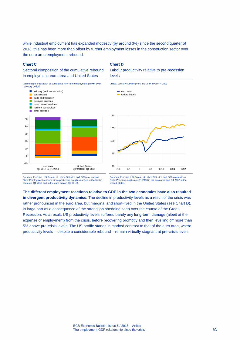
ECB Economic Bulletin, Issue 6 / 2016 – Article The employment-GDP relationship since the crisis 65
while industrial employment has expanded modestly (by around 3%) since the second quarter of 2013, this has been more than offset by further employment losses in the construction sector over the euro area employment rebound.
Chart D Labour productivity relative to pre-recession levels
(index: country-specific pre-crisis peak in GDP = 100)
Sources: Eurostat, US Bureau of Labor Statistics and ECB calculations. Note: Pre-crisis peaks are Q1 2008 in the euro area and Q4 2007 in the United States.
The different employment reactions relative to GDP in the two economies have also resulted in divergent productivity dynamics. The decline in productivity levels as a result of the crisis was rather pronounced in the euro area, but marginal and short-lived in the United States (see Chart D), in large part as a consequence of the strong job shedding seen over the course of the Great Recession. As a result, US productivity levels suffered barely any long-term damage (albeit at the expense of employment) from the crisis, before recovering promptly and then levelling off more than 5% above pre-crisis levels. The US profile stands in marked contrast to that of the euro area, where productivity levels – despite a considerable rebound – remain virtually stagnant at pre-crisis levels.
90
95
100
105
110
t-16 t-8 t t+8 t+16 t+24 t+32
euro areaUnited States
Chart C Sectoral composition of the cumulative rebound in employment: euro area and United States
(percentage breakdown of cumulative non-farm employment growth over recovery period)
Sources: Eurostat, US Bureau of Labor Statistics and ECB calculations. Note: Employment rebound since post-crisis trough (reached in the United States in Q1 2010 and in the euro area in Q2 2013).
-20
0
20
40
60
80
100
euro areaQ2 2013 to Q1 2016
United StatesQ2 2010 to Q1 2016
industry (excl. construction)constructiontrade and transportbusiness servicesother market servicesnon-market servicesother services

ECB Economic Bulletin, Issue 6 / 2016 – Article The employment-GDP relationship since the crisis 66
Chart F Growth in productivity per person employed and contributions: United States
(annual percentage changes; percentage point contributions)
Sources: US Bureau of Labor Statistics and ECB calculations.
Productivity growth, however, slowed markedly for both economies compared with pre-crisis averages. Following the trough reached in GDP in the second quarter of 2009, US annual productivity growth slowed to 0.9% year on year – more than halving its pre-crisis average rate of growth since 1999. In the euro area, where lower productivity growth has long been of concern to policymakers53, productivity growth slowed less (by around a third), but from a lower starting point, to just 0.6% year on year. More recently, since the euro area post-crisis rebound in GDP in the second quarter of 2013, the US productivity slowdown has been more marked still54 and is now virtually indistinguishable from the 0.4% year-on-year annual productivity growth seen in the euro area over this interval. In part, these slowdowns reflect a tendency towards stronger employment growth relative to GDP growth compared with the pre-crisis period – as shown in Charts E and F. Moreover, they reflect a notable and broadly-based decline in within-sector productivity growth across all economic sectors in both the euro area and in the United States.
The strong employment growth seen in both the euro area and the United States since the rebound in activity has been broadly welcomed by policymakers. Stronger employment growth has doubtless provided support to household incomes, but has also further weakened aggregate productivity growth, which was already notably weaker – even at the sectoral level – than in the pre-crisis period on both sides of the Atlantic. These common trends in productivity growth may imply risks to the long-term growth outlook in both economies.
53 See, for example, “On the importance of policy alignment to fulfil our economic potential”, 5th Annual
Tommaso Padoa-Schioppa Lecture by Mario Draghi, President of the ECB, at the Brussels Economic Forum 2016, 9 June, or the earlier special lecture at the 22nd Annual Congress of the European Economic Association entitled “Productivity in the euro area and monetary policy” by former ECB President, Jean-Claude Trichet (Budapest, 27 August 2007).
54 See also the box entitled “The slowdown in US labour productivity growth – stylised facts and economic implications”, Economic Bulletin, Issue 2, ECB, 2016.
-6
-4
-2
0
2
4
6
1999 2001 2003 2005 2007 2009 2011 2013 2015
real GDPemployment (inverted)productivity per person employedaverage pre-crisis productivity growth
Chart E Growth in productivity per person employed and contributions: euro area
(annual percentage changes; percentage point contributions)
Sources: Eurostat and ECB calculations.
-6
-4
-2
0
2
4
6
1999 2001 2003 2005 2007 2009 2011 2013 2015
real GDPemployment (inverted)productivity per person employedaverage pre-crisis productivity growth

ECB Economic Bulletin, Issue 6 / 2016 – Article The employment-GDP relationship since the crisis 67
The country dimension and the role of policy measures
So far, the rebound in euro area employment has been driven mainly by two large countries: Germany (where employment barely declined, even in the Great Recession) and Spain. These two countries have together accounted for around two-thirds of the cumulative increase in euro area employment since the trough in euro area employment reached in the second quarter of 2013 (31% and 25% respectively – see Chart 11).55 France and Italy have contributed much less to the euro area’s employment expansion (together accounting for just 13% of the expansion in employment seen since the first quarter of 2013), though in the past four quarters employment growth has also been gaining momentum in Italy. Meanwhile, employment growth has been relatively strong in several of the smaller – and formerly stressed – economies (most notably in Ireland and Portugal).
Chart 12 Employment elasticities: pre-crisis and to 2016
(estimated pre-crisis elasticities and post-crisis elasticities; x-axis: elasticity 1999-2008; y-axis: elasticity 1999-2016)
Sources: Eurostat and ECB calculations. Notes: Elasticities are computed by regressing quarter-on-quarter employment growth on quarter-on-quarter GDP growth (contemporaneous and up to four lags). All equations include an interaction term to account for the typical asymmetries associated with recessions (interacting a dummy variable, taking a value of 1 when the respective country was in recession, with the rate of quarter-on-quarter GDP growth), lagged dependent variables (to take account of the typical high degree of persistence in employment growth in many countries) and a constant. Country models were selected on the basis of their explanatory power (F-stat, R2) and the statistical significance of the estimated coefficients on GDP.
In the aftermath of the crisis, policy priorities have turned to means of spurring job growth, enhancing labour market flexibility and reducing long-standing labour market dualities. The aim is to aid reallocation and rebalancing – particularly in those countries most affected by strong job losses. Partly by design, these measures are likely to have influenced the elasticity of the response of employment to GDP growth in the recovery. In some countries, elasticities have peaked significantly during their respective recovery phases, reflecting the impact of ongoing
55 See also “What is behind the recent rebound in euro area employment?”, Economic Bulletin, 2015, op.
cit.
AT
BE
DEEE
ES
FR
IE
IT
LU
NL
PT
SI
SK
0
0.1
0.2
0.3
0.4
0.5
0.6
0.7
0.8
0.9
1
0 0.1 0.2 0.3 0.4 0.5 0.6 0.7 0.8 0.9 1
Chart 11 Country shares in cumulative euro area employment increase over the recovery
(share in euro area employment increase; percentages)
Sources: Eurostat and ECB calculations. Note: Country shares in the cumulative increase in euro area employment between Q1 2013 and Q1 2016 and 2015 share in euro area labour force.
0
5
10
15
20
25
30
35
DE FR IT ES others
share in the change in employmentlabour force share in 2015

ECB Economic Bulletin, Issue 6 / 2016 – Article The employment-GDP relationship since the crisis 68
structural reforms and shorter-term fiscal incentives to hiring. Chart 12 shows a broadly based increase in employment elasticities across most euro area countries since the crisis. The exploratory analysis in Chart 12 compares estimated employment elasticities at country level over the pre-crisis period with their post-crisis equivalents. Observations above the 45 degree line show those countries where post-crisis elasticities (estimated for the full Q1 1999 to Q1 2016 period) are significantly higher than their pre-crisis level (estimated from Q1 1999 to Q1 2008). Slightly more than half of the countries featured here show post-crisis employment elasticities notably higher than in the pre-crisis period.
The extent to which the drivers of recent increases in employment creation reflect ongoing structural changes or temporary fiscal measures will influence the likely persistence of the strong employment growth seen over the recovery. While a definitive assessment of their role is not yet possible given the short interval of the recovery in some countries56, structural changes – including the impact of structural reforms in several euro area economies (see Box 3 on “Recent employment dynamics and structural reforms”) – are likely to play a larger, sustained and more persistent role, also in those countries where temporary fiscal stimuli have helped to further boost employment creation over the recovery.57 Ongoing sectoral changes (in particular, the growing role of services in the national output of most euro area economies) and compositional effects leading to an increasingly flexible workforce58 are likely to result in a persistently stronger employment reaction to changes in output in most euro area economies in the post-crisis period.
Box 3 Recent employment dynamics and structural reforms
Structural reforms have the potential to alter the reaction of growth in employment to output growth.59 This may imply a direct change in the implied elasticities which capture the response of employment to GDP growth during the ongoing recovery – albeit one which is hard to isolate econometrically, given lags between the introduction and impact of reforms. This box presents some preliminary evidence regarding the impact of structural reforms on employment dynamics in euro area countries, with a particular focus on those countries which have implemented important product and labour market reforms.60
56 In Italy, for instance, the recovery in GDP has been evident for only five quarters (from the first quarter
of 2015 to the first quarter of 2016). 57 See also Sestito, P. and Viviano, E., “Hiring incentives and/or firing cost reduction? Evaluating the
impact of the 2015 policies on the Italian labour market”, Banca d’Italia Occasional Paper, No 325, March 2016.
58 Arising from growing shares of part-time employment and self-employment and, in several economies, temporary employment.
59 For a description of the main transmission channels of structural reforms, see “Progress with structural reforms across the euro area and their possible impacts”, Economic Bulletin, Issue 2, ECB, 2015.
60 At the same time, wage rigidities also seem to be present in a number of euro area economies and sectors, suggesting that firms’ capacity of adjustment to macroeconomic shocks may be limited across various dimensions. For recent evidence on wage rigidities, see the box entitled “Downward wage rigidity and the role of structural reforms in the euro area”, Economic Bulletin, Issue 8, ECB, 2015, or Anderton, R., Hantzsche, A., Savsek, S. and Tóth, M., “Sectoral Wage Rigidities and Labour and Product Market Institutions in the Euro Area”, CFCM Discussion Paper, 2016/01, Nottingham University, 2016.
ECB Economic Bulletin, Issue 6 / 2016 – Article The employment-GDP relationship since the crisis 69
Structural measures may have contributed to an increase in the responsiveness of employment to GDP during the recovery in several euro area countries. These include measures which increase labour market flexibility by decreasing excessive employment protection, for example by reducing severance payments or making wages more flexible. In consequence, firms in stressed economies may now consider it easier to adjust employment (Chart A). Firms in Greece and Spain appear to attribute easier employment adjustment mostly to labour market reforms.61 Meanwhile, product market reforms – including reforms which aim to reduce red tape or make it easier for new firms to enter the market, as well as those which reduce the protection of incumbent firms or professions – may also help to increase the speed or strength of employment adjustment of firms. All of these reforms are at least partly reflected in the change in product market regulation and employment protection legislation indicators which are plotted against recent changes in employment elasticities62 in Chart B. Overall, we see that countries which have implemented stronger structural reforms have also witnessed an increase in the responsiveness of employment to GDP over the course of the recovery.63
In countries where wide-ranging reforms were carried out earlier in response to the crisis, there is already some evidence of positive impacts on employment dynamics. For example, the 2012 labour market reform in Spain seems, at least partly, responsible for the country’s recent strong employment growth performance.64 At the same time, other factors – such as sectoral differences in growth rates and job creation, as well as a more pronounced rebound owing to previous substantial job losses in Spain – are also likely to have played a role. In Ireland, a package of effective active labour market policies has helped to significantly reduce the unemployment rate and get people back into work.65 In Greece, structural reforms in product and labour markets66
61 For details, see the results of the latest survey of the Wage Dynamics Network (WDN) in the box
entitled “Firms’ perceptions of changes in the ease of labour market adjustment and the role of reforms in stressed euro area countries during the period 2010-13 (based on the WDN3 survey)” in “New evidence on wage adjustment in Europe during the period 2010-13”, Economic Bulletin, Issue 5, ECB, 2016. See also the box entitled “Episodes of unemployment decline in the euro area and the role of structural reforms” in “Increasing resilience and long-term growth: the importance of sound institutions and economic structures for euro area countries and EMU”, Economic Bulletin, Issue 5, 2016, which shows that unemployment absorption episodes are often associated with a preceding period of structural reforms.
62 Elasticities are taken from a baseline model regressing quarter-on-quarter employment growth on quarter-on-quarter GDP growth (contemporaneous and up to four lags, according to the best-fit country lag structures suggested by the data). All equations include an interaction term to account for the typical asymmetries associated with recessions (interacting a dummy variable, taking a value of 1 when the respective country was in recession, with the rate of quarter-on-quarter GDP growth), up to two lagged dependent variables (to take account of the typical high degree of persistence in employment growth across many countries) and a constant. Country models were selected on the basis of their explanatory power (F-stat, R2) and the statistical significance of the variables of interest (estimated coefficients on GDP). The values reported in Chart A are corrected long-term values (i.e. adjusted for the lagged dependent variables).
63 This increased responsiveness seems particularly noteworthy given that the high levels of involuntary part-time employment during the crisis might have resulted in a weaker relationship between employment and output during the recovery if the additional working hours of part-timers had increased as well as employment (see, for example, “Comparisons and contrasts of the impact of the crisis on euro area labour markets”, Occasional Paper Series, op. cit., Section 2.4).
64 See Izquierdo, M., Lacuesta, A. and Puente, S., “The 2012 labour reform: an initial analysis of some of its effects on the labour market”, Economic Bulletin, Banco de España, September 2013, or Font, P., Izquierdo, M. and Puente, S., “Real wage responsiveness to unemployment in Spain: asymmetries along the business cycle”, IZA Journal of European Labor Studies, Vol. 4(13), June 2015.
65 At the same time, Ireland was considered a flexible economy already before the crisis. A quantification of the impact of the reforms can be found in “Quantification of the Economic Impacts of Selected Structural Reforms in Ireland”, IGEES Working Paper, July 2014.
66 For the impact of reforms in Greece, see for example IMF Country Report No 13/155, Selected Issues paper, June 2013, or “Assessing the Macroeconomic Impact of Structural Reforms in Greece”, Foundation for Economic & Industrial Research, March 2014.
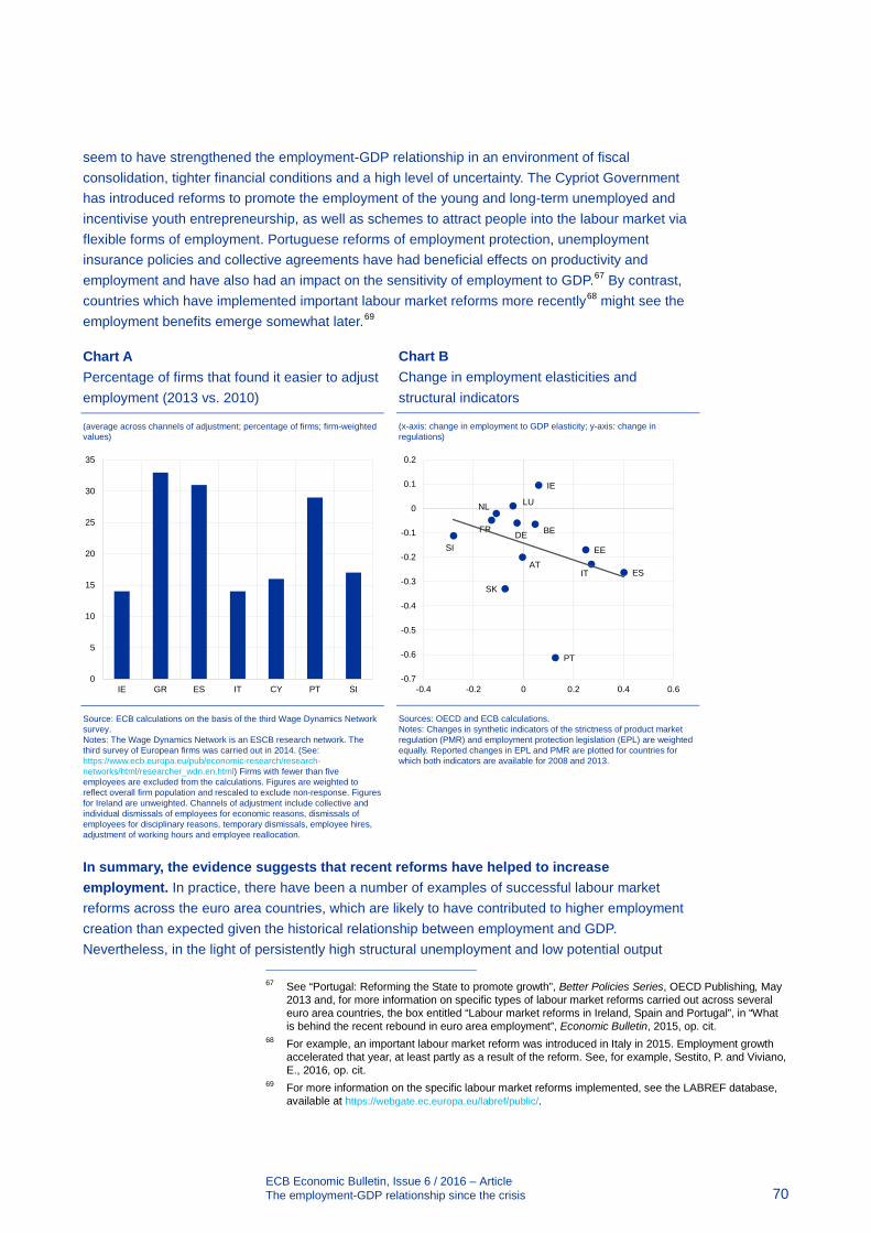
ECB Economic Bulletin, Issue 6 / 2016 – Article The employment-GDP relationship since the crisis 70
seem to have strengthened the employment-GDP relationship in an environment of fiscal consolidation, tighter financial conditions and a high level of uncertainty. The Cypriot Government has introduced reforms to promote the employment of the young and long-term unemployed and incentivise youth entrepreneurship, as well as schemes to attract people into the labour market via flexible forms of employment. Portuguese reforms of employment protection, unemployment insurance policies and collective agreements have had beneficial effects on productivity and employment and have also had an impact on the sensitivity of employment to GDP.67 By contrast, countries which have implemented important labour market reforms more recently68 might see the employment benefits emerge somewhat later.69
Chart B Change in employment elasticities and structural indicators
(x-axis: change in employment to GDP elasticity; y-axis: change in regulations)
Sources: OECD and ECB calculations. Notes: Changes in synthetic indicators of the strictness of product market regulation (PMR) and employment protection legislation (EPL) are weighted equally. Reported changes in EPL and PMR are plotted for countries for which both indicators are available for 2008 and 2013.
In summary, the evidence suggests that recent reforms have helped to increase employment. In practice, there have been a number of examples of successful labour market reforms across the euro area countries, which are likely to have contributed to higher employment creation than expected given the historical relationship between employment and GDP. Nevertheless, in the light of persistently high structural unemployment and low potential output
67 See “Portugal: Reforming the State to promote growth”, Better Policies Series, OECD Publishing, May
2013 and, for more information on specific types of labour market reforms carried out across several euro area countries, the box entitled “Labour market reforms in Ireland, Spain and Portugal”, in “What is behind the recent rebound in euro area employment”, Economic Bulletin, 2015, op. cit.
68 For example, an important labour market reform was introduced in Italy in 2015. Employment growth accelerated that year, at least partly as a result of the reform. See, for example, Sestito, P. and Viviano, E., 2016, op. cit.
69 For more information on the specific labour market reforms implemented, see the LABREF database, available at https://webgate.ec.europa.eu/labref/public/.
AT
BEDE
EE
ES
FR
IE
IT
LUNL
PT
SI
SK
-0.7
-0.6
-0.5
-0.4
-0.3
-0.2
-0.1
0
0.1
0.2
-0.4 -0.2 0 0.2 0.4 0.6
Chart A Percentage of firms that found it easier to adjust employment (2013 vs. 2010)
(average across channels of adjustment; percentage of firms; firm-weighted values)
Source: ECB calculations on the basis of the third Wage Dynamics Network survey. Notes: The Wage Dynamics Network is an ESCB research network. The third survey of European firms was carried out in 2014. (See: https://www.ecb.europa.eu/pub/economic-research/research-networks/html/researcher_wdn.en.html) Firms with fewer than five employees are excluded from the calculations. Figures are weighted to reflect overall firm population and rescaled to exclude non-response. Figures for Ireland are unweighted. Channels of adjustment include collective and individual dismissals of employees for economic reasons, dismissals of employees for disciplinary reasons, temporary dismissals, employee hires, adjustment of working hours and employee reallocation.
0
5
10
15
20
25
30
35
IE GR ES IT CY PT SI

ECB Economic Bulletin, Issue 6 / 2016 – Article The employment-GDP relationship since the crisis 71
growth in the euro area, the momentum of reforms needs to be stepped up in all euro area economies. Further product and labour market reforms will facilitate output and employment growth, while at the same time improving the capacity of euro area firms to adjust and thereby making the euro area more resilient to shocks.
Concluding remarks
The recovery in euro area activity has been accompanied by considerable employment creation. However, just 12 quarters after the post-crisis rebound in euro area GDP, it is still too early to tell whether the recent strong growth in employment is likely to remain a long-term feature of euro area labour markets. Nevertheless, it is worth noting that the two countries where output and employment growth have been the strongest since the recovery began – Germany and Spain – are among those which have carried out the widest-ranging reforms to their labour markets since the mid-2000s.70 The 2015 labour market reform in Italy has also helped spur renewed employment dynamism in the country over recent quarters. These observations may encourage other euro area countries to pursue further reforms.
To some extent, the recent strong employment growth seen in the euro area has been something of a positive surprise – to forecasters and policymakers alike. With the onset of the Great Recession in 2008, many had looked back at the strong pre-crisis rates of euro area employment growth as being the result of unsustainable sectoral imbalances in some countries, and thus unlikely to be repeated. However, over the post-crisis recovery, the euro area employment response to GDP growth appears to have been at least as strong as in the pre-crisis period – both at the aggregate level and in many of the euro area countries. This article suggests that the recent strong employment performance relative to GDP developments is partly due to structural changes under way across the euro area, including ongoing sectoral shifts and compositional changes to the workforce, which have resulted in a labour market that is more flexible and more responsive to cyclical dynamics.
70 In Germany, wide-ranging labour market reforms were enacted some years before the Great
Recession. These Hartz reforms have been widely credited for turning around the German labour market (see Dustmann, C., Fitzenberger, B., Schönberg, U., Spitz-Oener, A., “From Sick Man of Europe to Economic Superstar: Germany’s Resurgent Economy”, Journal of Economic Perspectives, Vol. 28, No 1, 2014). In Spain, reforms were first introduced in 2010, followed by a further and wider-reaching round in 2012. See The 2012 Labour Market Reform in Spain: A Preliminary Assessment, OECD, December 2013.
S 1ECB Economic Bulletin, Issue 6 / 2016 – Statistics
Statistics
S 1ECB Economic Bulletin, Issue 6 / 2016 - Statistics
Contents
1 External environment S 2
2 Financial developments S 3
3 Economic activity S 8
4 Prices and costs S 14
5 Money and credit S 18
6 Fiscal developments S 23
Further information
ECB statistics can be accessed from the Statistical Data Warehouse (SDW): http://sdw.ecb.europa.eu/
Data from the statistics section of the Economic Bulletin are available from the SDW: http://sdw.ecb.europa.eu/reports.do?node=1000004813
A comprehensive Statistics Bulletin can be found in the SDW: http://sdw.ecb.europa.eu/reports.do?node=1000004045
Methodological definitions can be found in the General Notes to the Statistics Bulletin: http://sdw.ecb.europa.eu/reports.do?node=10000023
Details on calculations can be found in the Technical Notes to the Statistics Bulletin: http://sdw.ecb.europa.eu/reports.do?node=10000022
Explanations of terms and abbreviations can be found in the ECBʼs statistics glossary: http://www.ecb.europa.eu/home/glossary/html/glossa.en.html
Conventions used in the tables
- data do not exist/data are not applicable . data are not yet available ... nil or negligible (p) provisional s.a. seasonally adjusted n.s.a. non-seasonally adjusted
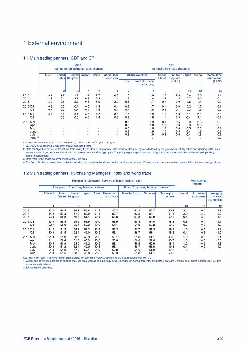
S 2ECB Economic Bulletin, Issue 6 / 2016 – Statistics
1 External environment
S 2ECB Economic Bulletin, Issue 6 / 2016 - Statistics
1.1 Main trading partners, GDP and CPI
GDP 1) CPI (period-on-period percentage changes) (annual percentage changes)
G20 2) United United Japan China Memo item: OECD countries United United Japan China Memo item:States Kingdom euro area States Kingdom euro area 3)
Total excluding food (HICP) (HICP)and energy
1 2 3 4 5 6 7 8 9 10 11 12 132013 3.1 1.7 1.9 1.4 7.7 -0.3 1.6 1.6 1.5 2.6 0.4 2.6 1.42014 3.3 2.4 3.1 -0.1 7.3 1.1 1.7 1.8 1.6 1.5 2.7 2.0 0.42015 3.2 2.6 2.2 0.6 6.9 2.0 0.6 1.7 0.1 0.0 0.8 1.4 0.02015 Q3 0.8 0.5 0.4 0.5 1.8 0.4 0.5 1.7 0.1 0.0 0.2 1.7 0.1 Q4 0.7 0.2 0.7 -0.4 1.5 0.4 0.7 1.8 0.5 0.1 0.3 1.5 0.22016 Q1 0.7 0.2 0.4 0.5 1.2 0.5 1.0 1.9 1.1 0.3 0.1 2.1 0.0 Q2 . 0.3 0.6 0.0 1.8 0.3 0.8 1.8 1.1 0.3 -0.4 2.1 -0.12016 Mar. - - - - - - 0.8 1.9 0.9 0.5 0.0 2.3 0.0 Apr. - - - - - - 0.8 1.8 1.1 0.3 -0.3 2.3 -0.2 May - - - - - - 0.8 1.8 1.0 0.3 -0.5 2.0 -0.1 June - - - - - - 0.9 1.9 1.0 0.5 -0.4 1.9 0.1 July - - - - - - 0.8 1.8 0.8 0.6 -0.4 1.8 0.2 Aug. 4) - - - - - - . . . . . . 0.2Sources: Eurostat (col. 3, 6, 10, 13); BIS (col. 2, 4, 9, 11, 12); OECD (col. 1, 5, 7, 8).1) Quarterly data seasonally adjusted; annual data unadjusted.2) Data for Argentina are currently not available owing to the state of emergency in the national statistical system declared by the government of Argentina on 7 January 2016. As a
consequence, Argentina is not included in the calculation of the G20 aggregate. The policy regarding the inclusion of Argentina will be reconsidered in the future depending onfurther developments.
3) Data refer to the changing composition of the euro area.4) The figure for the euro area is an estimate based on provisional national data, which usually cover around 95% of the euro area, as well as on early information on energy prices.
1.2 Main trading partners, Purchasing Managersʼ Index and world trade
Purchasing Managersʼ Surveys (diffusion indices; s.a.) Merchandise imports 1)
Composite Purchasing Managersʼ Index Global Purchasing Managersʼ Index 2)
Global 2) United United Japan China Memo item: Manufacturing Services New export Global Advanced EmergingStates Kingdom euro area orders economies market
economies
1 2 3 4 5 6 7 8 9 10 11 122013 53.4 54.8 56.8 52.6 51.5 49.7 52.2 52.7 50.6 3.1 -0.2 5.62014 54.2 57.3 57.9 50.9 51.1 52.7 53.2 54.1 51.4 2.9 3.9 2.22015 53.3 55.8 56.3 51.4 50.4 53.8 51.8 53.9 50.3 0.8 3.9 -1.42015 Q3 53.0 55.4 55.2 51.9 49.0 53.9 50.3 54.0 48.8 0.8 0.4 1.1 Q4 52.7 55.0 55.4 52.3 49.9 54.1 51.3 53.2 50.5 0.8 0.5 1.02016 Q1 51.2 51.5 54.2 51.2 50.3 53.2 50.7 51.3 49.4 -1.0 0.5 -2.1 Q2 50.8 51.5 52.4 49.0 50.5 53.1 49.7 51.1 48.8 -0.4 0.2 -1.02016 Mar. 51.0 51.3 53.6 49.9 51.3 53.1 51.0 51.1 49.3 -1.0 0.5 -2.1 Apr. 51.1 52.4 51.9 48.9 50.8 53.0 50.0 51.6 48.7 -1.0 0.8 -2.5 May 50.5 50.9 53.0 49.2 50.5 53.1 49.5 50.9 48.4 -1.2 -0.5 -1.8 June 50.6 51.2 52.4 49.0 50.3 53.1 49.7 51.0 49.3 -0.4 0.2 -1.0 July 51.2 51.8 47.6 50.1 51.9 53.2 51.6 51.0 49.7 . . . Aug. 51.3 51.5 53.6 49.8 51.8 52.9 51.8 51.1 50.3 . . . Sources: Markit (col. 1-9); CPB Netherlands Bureau for Economic Policy Analysis and ECB calculations (col. 10-12).1) Global and advanced economies exclude the euro area. Annual and quarterly data are period-on-period percentages; monthly data are 3-month-on-3-month percentages. All data
are seasonally adjusted.2) Excluding the euro area.
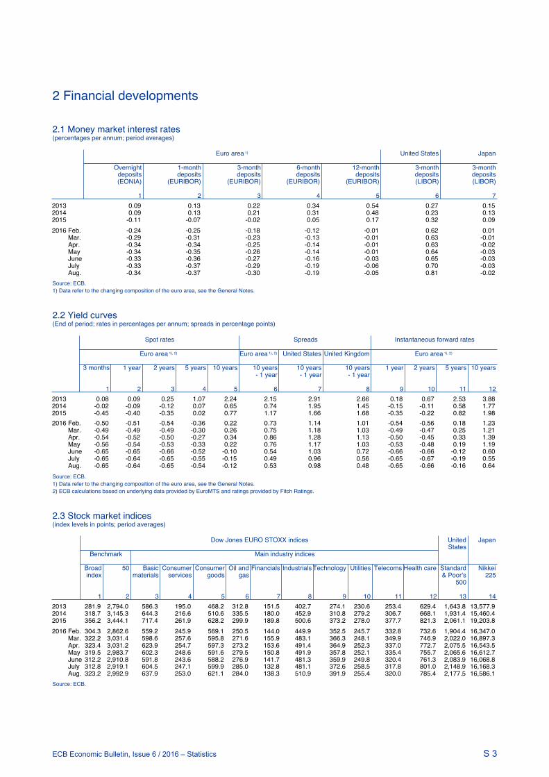
S 3ECB Economic Bulletin, Issue 6 / 2016 – Statistics
2 Financial developments
S 3ECB Economic Bulletin, Issue 6 / 2016 - Statistics
2.1 Money market interest rates(percentages per annum; period averages)
Euro area 1) United States Japan
Overnight 1-month 3-month 6-month 12-month 3-month 3-monthdeposits deposits deposits deposits deposits deposits deposits(EONIA) (EURIBOR) (EURIBOR) (EURIBOR) (EURIBOR) (LIBOR) (LIBOR)
1 2 3 4 5 6 72013 0.09 0.13 0.22 0.34 0.54 0.27 0.152014 0.09 0.13 0.21 0.31 0.48 0.23 0.132015 -0.11 -0.07 -0.02 0.05 0.17 0.32 0.092016 Feb. -0.24 -0.25 -0.18 -0.12 -0.01 0.62 0.01 Mar. -0.29 -0.31 -0.23 -0.13 -0.01 0.63 -0.01 Apr. -0.34 -0.34 -0.25 -0.14 -0.01 0.63 -0.02 May -0.34 -0.35 -0.26 -0.14 -0.01 0.64 -0.03 June -0.33 -0.36 -0.27 -0.16 -0.03 0.65 -0.03 July -0.33 -0.37 -0.29 -0.19 -0.06 0.70 -0.03 Aug. -0.34 -0.37 -0.30 -0.19 -0.05 0.81 -0.02Source: ECB.1) Data refer to the changing composition of the euro area, see the General Notes.
2.2 Yield curves(End of period; rates in percentages per annum; spreads in percentage points)
Spot rates Spreads Instantaneous forward rates
Euro area 1), 2) Euro area 1), 2) United States United Kingdom Euro area 1), 2)
3 months 1 year 2 years 5 years 10 years 10 years 10 years 10 years 1 year 2 years 5 years 10 years- 1 year - 1 year - 1 year
1 2 3 4 5 6 7 8 9 10 11 122013 0.08 0.09 0.25 1.07 2.24 2.15 2.91 2.66 0.18 0.67 2.53 3.882014 -0.02 -0.09 -0.12 0.07 0.65 0.74 1.95 1.45 -0.15 -0.11 0.58 1.772015 -0.45 -0.40 -0.35 0.02 0.77 1.17 1.66 1.68 -0.35 -0.22 0.82 1.982016 Feb. -0.50 -0.51 -0.54 -0.36 0.22 0.73 1.14 1.01 -0.54 -0.56 0.18 1.23 Mar. -0.49 -0.49 -0.49 -0.30 0.26 0.75 1.18 1.03 -0.49 -0.47 0.25 1.21 Apr. -0.54 -0.52 -0.50 -0.27 0.34 0.86 1.28 1.13 -0.50 -0.45 0.33 1.39 May -0.56 -0.54 -0.53 -0.33 0.22 0.76 1.17 1.03 -0.53 -0.48 0.19 1.19 June -0.65 -0.65 -0.66 -0.52 -0.10 0.54 1.03 0.72 -0.66 -0.66 -0.12 0.60 July -0.65 -0.64 -0.65 -0.55 -0.15 0.49 0.96 0.56 -0.65 -0.67 -0.19 0.55 Aug. -0.65 -0.64 -0.65 -0.54 -0.12 0.53 0.98 0.48 -0.65 -0.66 -0.16 0.64Source: ECB.1) Data refer to the changing composition of the euro area, see the General Notes.2) ECB calculations based on underlying data provided by EuroMTS and ratings provided by Fitch Ratings.
2.3 Stock market indices(index levels in points; period averages)
Dow Jones EURO STOXX indices United Japan States
Benchmark Main industry indices
Broad 50 Basic Consumer Consumer Oil and Financials Industrials Technology Utilities Telecoms Health care Standard Nikkeiindex materials services goods gas & Poorʼs 225
500
1 2 3 4 5 6 7 8 9 10 11 12 13 142013 281.9 2,794.0 586.3 195.0 468.2 312.8 151.5 402.7 274.1 230.6 253.4 629.4 1,643.8 13,577.92014 318.7 3,145.3 644.3 216.6 510.6 335.5 180.0 452.9 310.8 279.2 306.7 668.1 1,931.4 15,460.42015 356.2 3,444.1 717.4 261.9 628.2 299.9 189.8 500.6 373.2 278.0 377.7 821.3 2,061.1 19,203.82016 Feb. 304.3 2,862.6 559.2 245.9 569.1 250.5 144.0 449.9 352.5 245.7 332.8 732.6 1,904.4 16,347.0 Mar. 322.2 3,031.4 598.6 257.6 595.8 271.6 155.9 483.1 366.3 248.1 349.9 746.9 2,022.0 16,897.3 Apr. 323.4 3,031.2 623.9 254.7 597.3 273.2 153.6 491.4 364.9 252.3 337.0 772.7 2,075.5 16,543.5 May 319.5 2,983.7 602.3 248.6 591.6 279.5 150.8 491.9 357.8 252.1 335.4 755.7 2,065.6 16,612.7 June 312.2 2,910.8 591.8 243.6 588.2 276.9 141.7 481.3 359.9 249.8 320.4 761.3 2,083.9 16,068.8 July 312.8 2,919.1 604.5 247.1 599.9 285.0 132.8 481.1 372.6 258.5 317.8 801.0 2,148.9 16,168.3 Aug. 323.2 2,992.9 637.9 253.0 621.1 284.0 138.3 510.9 391.9 255.4 320.0 785.4 2,177.5 16,586.1Source: ECB.
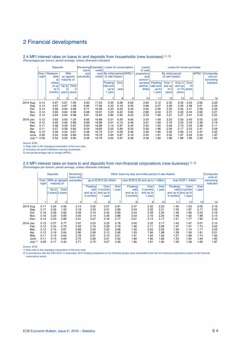
S 4ECB Economic Bulletin, Issue 6 / 2016 – Statistics
2 Financial developments
S 4ECB Economic Bulletin, Issue 6 / 2016 - Statistics
2.4 MFI interest rates on loans to and deposits from households (new business) 1), 2)(Percentages per annum; period average, unless otherwise indicated)
Deposits Revolving Extended Loans for consumption Loans Loans for house purchase
loans credit to sole Over- Redeem- With and card By initial period APRC 3) proprietors By initial period APRC 3) Compositenight able an agreed overdrafts credit of rate fixation and of rate fixation cost-of-
at maturity of: unincor- borrowingnotice Floating Over porated Floating Over 1 Over 5 Over indicatorof up Up to Over rate and 1 partner- rate and and up and up 10to 3 2 2 up to year ships up to to 5 to 10 years
months years years 1 year 1 year years years
1 2 3 4 5 6 7 8 9 10 11 12 13 14 15 162015 Aug. 0.14 0.67 0.67 1.00 6.83 17.03 5.30 6.28 6.62 2.60 2.12 2.35 2.30 2.33 2.60 2.26 Sep. 0.14 0.67 0.67 1.08 6.85 17.06 5.22 6.18 6.55 2.68 2.07 2.36 2.29 2.38 2.61 2.25 Oct. 0.14 0.66 0.64 0.99 6.71 16.98 5.22 6.03 6.43 2.64 2.06 2.32 2.30 2.41 2.58 2.26 Nov. 0.14 0.65 0.64 0.96 6.68 16.91 5.23 6.22 6.60 2.68 2.04 2.31 2.32 2.45 2.62 2.27 Dec. 0.13 0.64 0.64 0.98 6.61 16.95 4.84 5.94 6.25 2.53 1.99 2.27 2.27 2.41 2.55 2.222016 Jan. 0.12 0.62 0.63 1.25 6.65 16.88 5.31 6.29 6.65 2.53 1.99 2.22 2.30 2.40 2.53 2.23 Feb. 0.12 0.60 0.60 0.89 6.66 16.89 5.01 6.13 6.46 2.61 1.99 2.19 2.23 2.33 2.48 2.19 Mar. 0.11 0.58 0.59 0.87 6.63 16.88 5.14 5.97 6.34 2.53 1.90 2.09 2.10 2.24 2.38 2.11 Apr. 0.11 0.57 0.58 0.85 6.54 16.82 5.20 5.99 6.33 2.56 1.86 2.09 2.17 2.23 2.41 2.09 May 0.10 0.56 0.54 0.87 6.56 16.75 5.21 6.09 6.46 2.56 1.85 2.02 2.06 2.12 2.37 2.02 June 0.09 0.54 0.56 0.86 6.55 16.79 4.94 5.87 6.18 2.44 1.81 2.00 1.97 2.02 2.32 1.97 July (p) 0.09 0.52 0.50 0.92 6.46 16.79 5.04 5.97 6.28 2.39 1.82 1.96 1.96 1.96 2.32 1.92Source: ECB.1) Data refer to the changing composition of the euro area.2) Including non-profit institutions serving households.3) Annual percentage rate of charge (APRC).
2.5 MFI interest rates on loans to and deposits from non-financial corporations (new business) 1), 2)(Percentages per annum; period average, unless otherwise indicated)
Deposits Revolving Other loans by size and initial period of rate fixation Composite
loans and cost-of-Over- With an agreed overdrafts up to EUR 0.25 million over EUR 0.25 and up to 1 million over EUR 1 million borrowingnight maturity of: indicator
Floating Over Over Floating Over Over Floating Over OverUp to Over rate 3 months 1 year rate 3 months 1 year rate 3 months 1 year
2 years 2 years and up to and up to and up to and up to and up to and up to3 months 1 year 3 months 1 year 3 months 1 year
1 2 3 4 5 6 7 8 9 10 11 12 13 142015 Aug. 0.17 0.24 0.92 3.14 3.25 3.57 2.91 2.07 2.32 2.22 1.45 1.53 2.03 2.16 Sep. 0.17 0.26 1.00 3.18 3.23 3.51 2.89 2.04 2.25 2.21 1.55 1.87 2.17 2.23 Oct. 0.16 0.26 0.82 3.09 3.19 3.42 2.89 2.04 2.28 2.20 1.48 1.69 2.03 2.16 Nov. 0.16 0.23 0.83 3.05 3.14 3.39 2.88 2.03 2.16 2.20 1.46 1.62 1.98 2.13 Dec. 0.14 0.23 0.85 3.01 3.07 3.18 2.77 2.01 2.13 2.17 1.51 1.77 1.92 2.102016 Jan. 0.13 0.27 0.77 2.97 3.23 3.25 2.78 2.00 2.22 2.17 1.43 1.67 2.07 2.10 Feb. 0.13 0.24 0.70 2.93 3.16 3.28 2.76 1.96 2.11 2.09 1.37 1.47 1.74 2.02 Mar. 0.13 0.16 0.87 2.89 3.03 3.20 2.68 1.92 2.03 2.02 1.39 1.74 1.77 2.05 Apr. 0.12 0.19 0.64 2.80 2.99 3.12 2.66 1.93 1.96 1.98 1.38 1.59 1.81 2.01 May 0.11 0.13 0.63 2.76 2.91 3.10 2.61 1.91 1.94 1.92 1.27 1.68 1.74 1.92 June 0.11 0.15 0.64 2.75 2.66 3.01 2.52 1.85 1.90 1.85 1.34 1.60 1.64 1.90 July (p) 0.09 0.17 0.42 2.71 2.72 3.07 2.48 1.86 1.91 1.82 1.28 1.58 1.69 1.87Source: ECB.1) Data refer to the changing composition of the euro area.2) In accordance with the ESA 2010, in December 2014 holding companies of non-financial groups were reclassified from the non-financial corporations sector to the financial
corporations sector.

S 5ECB Economic Bulletin, Issue 6 / 2016 – Statistics
2 Financial developments
S 5ECB Economic Bulletin, Issue 6 / 2016 - Statistics
2.6 Debt securities issued by euro area residents, by sector of the issuer and initial maturity(EUR billions; transactions during the month and end-of-period outstanding amounts; nominal values)
Short-term
Outstanding amounts Gross issues 1)
Total MFIs Non-MFI corporations General government Total MFIs Non-MFI corporations General government
(including (including Euro- Financial Non- Central Other Euro- Financial Non- Central Other
system) corporations financial govern- general system) corporations financial govern- generalother than FVCs corporations ment govern- other than FVCs corporations ment govern-
MFIs ment MFIs ment
1 2 3 4 5 6 7 8 9 10 11 12 13 14
2013 1,255 483 124 . 67 529 53 508 314 31 . 44 99 212014 1,318 543 129 . 59 538 50 410 219 34 . 38 93 252015 1,262 517 140 . 61 478 65 336 150 37 . 32 82 342016 Jan. 1,284 524 142 . 68 483 67 329 141 35 . 33 87 33 Feb. 1,302 536 142 . 71 487 66 318 144 32 . 30 81 31 Mar. 1,283 515 135 . 72 493 69 321 123 38 . 30 89 40 Apr. 1,285 519 126 . 78 495 68 352 155 36 . 33 82 46 May 1,295 530 123 . 79 495 68 333 153 37 . 34 75 34 June 1,279 526 123 . 67 494 69 307 136 37 . 28 80 27
Long-term2013 15,113 4,403 3,092 . 921 6,069 628 222 70 39 . 16 89 92014 15,132 4,046 3,164 . 995 6,285 642 220 65 44 . 16 85 102015 15,244 3,784 3,276 . 1,066 6,481 637 214 67 44 . 13 81 92016 Jan. 15,218 3,753 3,256 . 1,053 6,521 634 207 75 25 . 7 93 8 Feb. 15,155 3,751 3,175 . 1,047 6,549 633 209 66 42 . 4 88 10 Mar. 15,156 3,728 3,128 . 1,057 6,604 639 248 72 39 . 26 94 17 Apr. 15,120 3,724 3,142 . 1,073 6,548 633 219 61 35 . 25 91 7 May 15,231 3,732 3,157 . 1,097 6,611 634 238 59 49 . 34 88 8 June 15,272 3,733 3,141 . 1,096 6,663 638 214 72 41 . 13 79 10Source: ECB.1) For the purpose of comparison, annual data refer to the average monthly figure over the year.
2.7 Growth rates and outstanding amounts of debt securities and listed shares(EUR billions; percentage changes)
Oustanding amount
Debt securities Listed shares
Total MFIs Non-MFI corporations General government Total MFIs Financial Non-
(including corporations financialEurosystem) Financial Non- Central Other other than corporations
corporations financial government general MFIsother than FVCs corporations government
MFIs
1 2 3 4 5 6 7 8 9 10 11
2013 16,367.8 4,886.3 3,215.9 . 987.4 6,598.1 680.0 5,649.0 569.1 742.5 4,337.42014 16,450.2 4,588.1 3,292.9 . 1,053.3 6,823.2 692.7 5,958.0 591.1 780.6 4,586.32015 16,505.9 4,301.4 3,416.2 . 1,127.2 6,959.3 701.9 6,744.7 586.1 911.6 5,247.02016 Jan. 16,502.3 4,277.8 3,397.7 . 1,120.9 7,004.9 701.1 6,343.7 490.7 858.0 4,995.0 Feb. 16,457.0 4,286.8 3,317.5 . 1,117.3 7,036.4 698.9 6,240.5 471.7 877.4 4,891.5 Mar. 16,438.9 4,243.5 3,263.2 . 1,128.3 7,096.7 707.2 6,419.6 483.4 902.0 5,034.2 Apr. 16,404.8 4,243.3 3,268.1 . 1,150.7 7,042.5 700.2 6,462.3 505.5 917.5 5,039.4 May 16,525.9 4,262.2 3,279.1 . 1,176.3 7,106.6 701.6 6,552.4 491.5 923.2 5,137.7 June 16,550.7 4,258.9 3,264.4 . 1,163.6 7,156.4 707.3 6,204.6 395.0 861.7 4,948.0
Growth rate2013 -1.4 -8.9 -3.3 . 8.0 4.5 -1.1 0.7 7.2 -0.4 0.22014 -0.7 -7.9 0.4 . 5.1 3.1 1.1 1.5 7.2 1.2 0.72015 0.2 -6.9 5.1 . 5.3 1.8 0.6 1.1 4.5 1.5 0.62016 Jan. -0.3 -7.7 3.6 . 4.4 2.0 0.7 1.0 3.3 1.5 0.7 Feb. -0.7 -7.1 1.2 . 2.8 2.0 -0.4 1.0 3.3 1.2 0.7 Mar. -0.9 -6.9 -0.9 . 3.3 2.2 0.2 0.9 3.3 1.5 0.6 Apr. -0.9 -6.8 -0.3 . 4.0 1.7 -0.1 0.9 2.6 1.8 0.6 May -0.7 -5.9 -0.9 . 6.0 1.6 0.6 0.9 2.5 1.6 0.6 June -0.2 -4.6 -1.8 . 6.0 2.2 2.7 0.9 2.7 1.6 0.6Source: ECB.

S 6ECB Economic Bulletin, Issue 6 / 2016 – Statistics
2 Financial developments
S 6ECB Economic Bulletin, Issue 6 / 2016 - Statistics
2.8 Effective exchange rates 1)(period averages; index: 1999 Q1=100)
EER-19 EER-38
Nominal Real CPI Real PPI Real GDP Real ULCM 2) Real ULCT Nominal Real CPIdeflator
1 2 3 4 5 6 7 82013 101.2 98.2 96.7 91.1 101.0 99.1 111.9 95.52014 101.8 97.8 96.8 91.2 100.8 100.5 114.7 96.02015 92.4 88.4 89.1 83.4 89.5 91.5 106.5 87.82015 Q3 92.7 88.7 89.6 83.8 90.2 91.9 107.6 88.5 Q4 92.4 88.3 89.3 83.9 88.8 91.4 107.7 88.32016 Q1 94.1 89.5 90.8 85.4 90.0 92.3 110.4 90.1 Q2 94.9 90.3 91.5 . . . 110.8 90.42016 Mar. 94.1 89.5 90.8 - - - 110.0 89.9 Apr. 94.8 90.1 91.4 - - - 110.6 90.2 May 95.1 90.5 91.7 - - - 111.1 90.7 June 94.7 90.2 91.3 - - - 110.5 90.3 July 94.9 90.3 91.6 - - - 110.2 89.8 Aug. 95.2 90.6 92.0 - - - 110.6 90.1
Percentage change versus previous month2016 Aug. 0.3 0.3 0.4 - - - 0.4 0.3
Percentage change versus previous year2016 Aug. 2.3 1.8 2.4 - - - 2.4 1.3Source: ECB.1) For a definition of the trading partner groups and other information see the General Notes to the Statistics Bulletin.2) ULCM-deflated series are available only for the EER-18 trading partner group.
2.9 Bilateral exchange rates(period averages; units of national currency per euro)
Chinese Croatian Czech Danish Hungarian Japanese Polish Pound Romanian Swedish Swiss USrenminbi kuna koruna krone forint yen zloty sterling leu krona franc Dollar
1 2 3 4 5 6 7 8 9 10 11 122013 8.165 7.579 25.980 7.458 296.873 129.663 4.197 0.849 4.4190 8.652 1.231 1.3282014 8.186 7.634 27.536 7.455 308.706 140.306 4.184 0.806 4.4437 9.099 1.215 1.3292015 6.973 7.614 27.279 7.459 309.996 134.314 4.184 0.726 4.4454 9.353 1.068 1.1102015 Q3 7.008 7.578 27.075 7.462 312.095 135.863 4.188 0.717 4.4290 9.429 1.072 1.112 Q4 7.000 7.623 27.057 7.460 312.652 132.952 4.264 0.722 4.4573 9.302 1.085 1.0952016 Q1 7.210 7.617 27.040 7.461 312.024 126.997 4.365 0.770 4.4924 9.327 1.096 1.102 Q2 7.379 7.504 27.040 7.439 313.371 121.949 4.372 0.787 4.4986 9.278 1.096 1.1292016 Mar. 7.222 7.559 27.051 7.457 311.154 125.385 4.293 0.780 4.4666 9.285 1.092 1.110 Apr. 7.346 7.495 27.031 7.443 311.462 124.287 4.311 0.792 4.4724 9.203 1.093 1.134 May 7.386 7.498 27.026 7.439 314.581 123.214 4.404 0.778 4.4991 9.295 1.106 1.131 June 7.402 7.520 27.061 7.437 313.984 118.453 4.400 0.790 4.5230 9.334 1.089 1.123 July 7.391 7.493 27.042 7.439 314.353 115.250 4.396 0.841 4.4856 9.474 1.087 1.107 Aug. 7.454 7.487 27.025 7.441 310.205 113.487 4.300 0.855 4.4591 9.491 1.088 1.121
Percentage change versus previous month2016 Aug. 0.8 -0.1 -0.1 0.0 -1.3 -1.5 -2.2 1.7 -0.6 0.2 0.1 1.3
Percentage change versus previous year2016 Aug. 5.5 -0.9 -0.1 -0.3 -0.5 -17.2 2.5 19.7 0.8 -0.3 1.0 0.7Source: ECB.

S 7ECB Economic Bulletin, Issue 6 / 2016 – Statistics
2 Financial developments
S 7ECB Economic Bulletin, Issue 6 / 2016 - Statistics
2.10 Euro area balance of payments, financial account(EUR billions, unless otherwise indicated; outstanding amounts at end of period; transactions during period)
Outstanding amounts (international investment position)
Total 1) Direct Portfolio Net Other investment Reserve Memo:
investment investment financial assets Grossderivatives external
Assets Liabilities Net Assets Liabilities Assets Liabilities Assets Liabilities debt
1 2 3 4 5 6 7 8 9 10 11 12
2015 Q2 22,097.0 23,303.8 -1,206.8 9,376.5 7,521.5 7,195.1 10,684.5 -29.3 4,896.2 5,097.9 658.5 13,264.2 Q3 21,671.7 22,842.6 -1,170.9 9,391.6 7,625.3 6,854.1 10,158.7 -36.3 4,818.1 5,058.6 644.2 13,116.6 Q4 22,191.1 23,156.8 -965.7 9,747.6 7,960.0 7,178.8 10,282.5 -28.3 4,648.8 4,914.3 644.2 12,962.32016 Q1 22,117.4 23,375.2 -1,257.7 9,683.3 8,217.7 7,097.5 10,059.8 -28.0 4,689.4 5,097.6 675.3 13,287.1
Outstanding amounts as a percentage of GDP2016 Q1 210.1 222.1 -12.0 92.0 78.1 67.4 95.6 -0.3 44.6 48.4 6.4 126.2
Transactions2015 Q3 90.0 32.3 57.7 114.0 124.4 25.5 -68.8 -1.2 -51.0 -23.3 2.7 - Q4 106.6 -64.0 170.6 181.3 142.0 105.4 -16.1 54.2 -238.9 -190.0 4.6 -2016 Q1 433.4 384.6 48.9 165.7 122.1 135.0 -7.7 18.6 113.3 270.1 1.0 - Q2 311.2 162.9 148.3 68.6 19.6 141.5 -6.2 -7.5 106.5 149.6 2.2 -2016 Jan. 234.1 250.5 -16.4 37.4 69.3 35.8 -51.2 14.8 147.1 232.3 -1.2 - Feb. 176.9 182.4 -5.5 84.3 39.3 47.2 13.1 6.8 37.5 130.0 1.1 - Mar. 22.5 -48.3 70.8 44.0 13.5 51.9 30.4 -3.1 -71.3 -92.2 1.1 - Apr. 185.4 142.6 42.8 19.8 11.9 73.3 -47.8 -6.1 100.0 178.5 -1.6 - May 142.0 96.3 45.7 59.7 21.1 30.5 22.9 -0.5 49.2 52.4 3.1 - June -16.3 -76.0 59.8 -10.9 -13.3 37.6 18.6 -0.9 -42.8 -81.3 0.7 -
12-month cumulated transactions2016 June 941.3 515.8 425.5 529.6 408.2 407.4 -98.8 64.1 -70.2 206.4 10.4 -
12-month cumulated transactions as a percentage of GDP2016 June 8.9 4.9 4.0 5.0 3.8 3.8 -0.9 0.6 -0.7 1.9 0.1 -Source: ECB.1) Net financial derivatives are included in total assets.

S 8ECB Economic Bulletin, Issue 6 / 2016 – Statistics
3 Economic activity
S 8ECB Economic Bulletin, Issue 6 / 2016 - Statistics
3.1 GDP and expenditure components(quarterly data seasonally adjusted; annual data unadjusted)
Current prices (EUR billions)
GDP
Total Domestic demand External balance 1)
Total Private Government Gross fixed capital formation Changes in Total Exports 1) Imports 1)
consumption consumption inventories 2)
Total Total Intellectualconstruction machinery property
products
1 2 3 4 5 6 7 8 9 10 11 12
2013 9,938.2 9,607.0 5,561.7 2,093.9 1,951.3 1,004.3 573.1 366.7 0.1 331.2 4,373.9 4,042.72014 10,127.6 9,768.4 5,634.1 2,124.5 1,991.7 1,007.4 595.7 376.3 18.1 359.2 4,533.1 4,173.92015 10,454.6 9,976.3 5,741.1 2,163.8 2,069.1 1,022.2 630.9 398.3 2.3 478.3 4,826.5 4,348.22015 Q3 2,619.3 2,498.2 1,440.8 542.4 516.9 254.2 156.7 101.4 -2.0 121.1 1,210.4 1,089.3 Q4 2,643.3 2,521.8 1,447.0 546.1 526.8 257.9 162.9 100.6 1.9 121.5 1,214.6 1,093.02016 Q1 2,659.7 2,532.3 1,451.6 551.2 528.3 260.9 164.4 101.8 1.1 127.4 1,196.4 1,069.0 Q2 2,674.4 2,540.7 1,459.7 553.7 528.7 . . . -1.3 133.8 1,209.9 1,076.1
as a percentage of GDP2015 100.0 95.4 54.9 20.7 19.8 9.8 6.0 3.8 0.0 4.6 - -
Chain-linked volumes (prices for the previous year)quarter-on-quarter percentage changes
2015 Q3 0.4 0.7 0.5 0.4 0.5 0.2 0.5 1.2 - - 0.4 1.2 Q4 0.4 0.7 0.3 0.6 1.4 1.3 3.2 -0.9 - - 0.7 1.42016 Q1 0.5 0.4 0.6 0.6 0.4 0.7 1.1 0.7 - - 0.0 -0.1 Q2 0.3 -0.1 0.2 0.1 0.0 . . . - - 1.1 0.4
annual percentage changes2013 -0.3 -0.6 -0.6 0.2 -2.4 -3.6 -2.5 0.1 - - 2.2 1.52014 1.1 1.1 0.8 0.6 1.5 -0.5 4.1 2.1 - - 4.4 4.82015 2.0 1.9 1.8 1.4 3.1 1.0 5.1 4.6 - - 6.3 6.32015 Q3 2.0 1.9 1.9 1.3 2.7 0.7 3.2 6.6 - - 5.7 5.9 Q4 2.0 2.3 1.7 1.9 3.7 1.8 6.1 4.1 - - 4.8 5.82016 Q1 1.7 2.1 1.9 2.0 2.5 1.3 5.1 3.6 - - 2.3 3.2 Q2 1.6 1.9 1.7 1.8 2.4 . . . - - 2.2 2.8
contributions to quarter-on-quarter percentage changes in GDP; percentage points2015 Q3 0.4 0.7 0.3 0.1 0.1 0.0 0.0 0.0 0.2 -0.3 - - Q4 0.4 0.7 0.2 0.1 0.3 0.1 0.2 0.0 0.1 -0.3 - - 2016 Q1 0.5 0.4 0.3 0.1 0.1 0.1 0.1 0.0 -0.1 0.1 - - Q2 0.3 -0.1 0.1 0.0 0.0 . . . -0.2 0.4 - -
contributions to annual percentage changes in GDP; percentage points2013 -0.3 -0.6 -0.3 0.0 -0.5 -0.4 -0.2 0.0 0.2 0.4 - - 2014 1.1 1.1 0.4 0.1 0.3 -0.1 0.2 0.1 0.2 0.0 - - 2015 2.0 1.8 1.0 0.3 0.6 0.1 0.3 0.2 -0.1 0.2 - - 2015 Q3 2.0 1.9 1.0 0.3 0.5 0.1 0.2 0.2 0.0 0.1 - - Q4 2.0 2.2 0.9 0.4 0.7 0.2 0.4 0.2 0.2 -0.2 - - 2016 Q1 1.7 1.9 1.0 0.4 0.5 0.1 0.3 0.1 0.0 -0.3 - - Q2 1.6 1.8 0.9 0.4 0.5 . . . 0.0 -0.2 - - Sources: Eurostat and ECB calculations.1) Exports and imports cover goods and services and include cross-border intra-euro area trade.2) Including acquisitions less disposals of valuables.
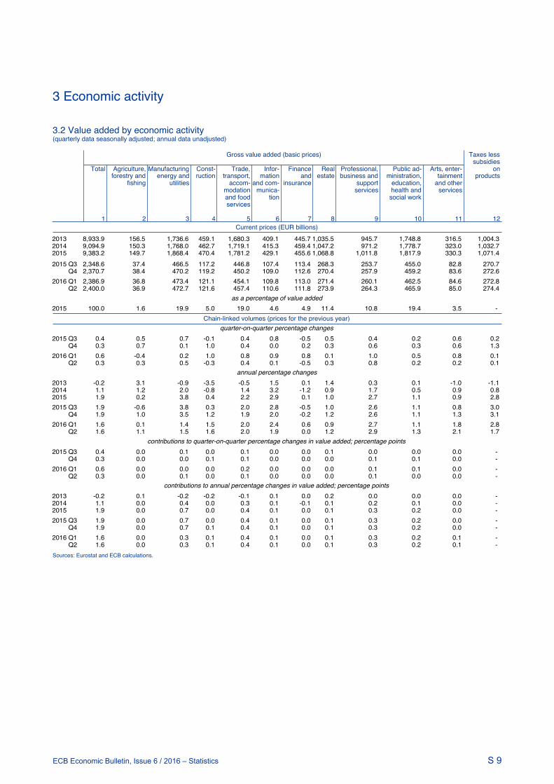
S 9ECB Economic Bulletin, Issue 6 / 2016 – Statistics
3 Economic activity
S 9ECB Economic Bulletin, Issue 6 / 2016 - Statistics
3.2 Value added by economic activity(quarterly data seasonally adjusted; annual data unadjusted)
Current prices (EUR billions)
Gross value added (basic prices) Taxes lesssubsidies
Total Agriculture, Manufacturing Const- Trade, Infor- Finance Real Professional, Public ad- Arts, enter- onforestry and energy and ruction transport, mation and estate business and ministration, tainment products
fishing utilities accom- and com- insurance support education, and othermodation munica- services health and servicesand food tion social workservices
1 2 3 4 5 6 7 8 9 10 11 12
2013 8,933.9 156.5 1,736.6 459.1 1,680.3 409.1 445.7 1,035.5 945.7 1,748.8 316.5 1,004.32014 9,094.9 150.3 1,768.0 462.7 1,719.1 415.3 459.4 1,047.2 971.2 1,778.7 323.0 1,032.72015 9,383.2 149.7 1,868.4 470.4 1,781.2 429.1 455.6 1,068.8 1,011.8 1,817.9 330.3 1,071.42015 Q3 2,348.6 37.4 466.5 117.2 446.8 107.4 113.4 268.3 253.7 455.0 82.8 270.7 Q4 2,370.7 38.4 470.2 119.2 450.2 109.0 112.6 270.4 257.9 459.2 83.6 272.62016 Q1 2,386.9 36.8 473.4 121.1 454.1 109.8 113.0 271.4 260.1 462.5 84.6 272.8 Q2 2,400.0 36.9 472.7 121.6 457.4 110.6 111.8 273.9 264.3 465.9 85.0 274.4
as a percentage of value added2015 100.0 1.6 19.9 5.0 19.0 4.6 4.9 11.4 10.8 19.4 3.5 -
Chain-linked volumes (prices for the previous year)quarter-on-quarter percentage changes
2015 Q3 0.4 0.5 0.7 -0.1 0.4 0.8 -0.5 0.5 0.4 0.2 0.6 0.2 Q4 0.3 0.7 0.1 1.0 0.4 0.0 0.2 0.3 0.6 0.3 0.6 1.32016 Q1 0.6 -0.4 0.2 1.0 0.8 0.9 0.8 0.1 1.0 0.5 0.8 0.1 Q2 0.3 0.3 0.5 -0.3 0.4 0.1 -0.5 0.3 0.8 0.2 0.2 0.1
annual percentage changes2013 -0.2 3.1 -0.9 -3.5 -0.5 1.5 0.1 1.4 0.3 0.1 -1.0 -1.12014 1.1 1.2 2.0 -0.8 1.4 3.2 -1.2 0.9 1.7 0.5 0.9 0.82015 1.9 0.2 3.8 0.4 2.2 2.9 0.1 1.0 2.7 1.1 0.9 2.82015 Q3 1.9 -0.6 3.8 0.3 2.0 2.8 -0.5 1.0 2.6 1.1 0.8 3.0 Q4 1.9 1.0 3.5 1.2 1.9 2.0 -0.2 1.2 2.6 1.1 1.3 3.12016 Q1 1.6 0.1 1.4 1.5 2.0 2.4 0.6 0.9 2.7 1.1 1.8 2.8 Q2 1.6 1.1 1.5 1.6 2.0 1.9 0.0 1.2 2.9 1.3 2.1 1.7
contributions to quarter-on-quarter percentage changes in value added; percentage points2015 Q3 0.4 0.0 0.1 0.0 0.1 0.0 0.0 0.1 0.0 0.0 0.0 - Q4 0.3 0.0 0.0 0.1 0.1 0.0 0.0 0.0 0.1 0.1 0.0 - 2016 Q1 0.6 0.0 0.0 0.0 0.2 0.0 0.0 0.0 0.1 0.1 0.0 - Q2 0.3 0.0 0.1 0.0 0.1 0.0 0.0 0.0 0.1 0.0 0.0 -
contributions to annual percentage changes in value added; percentage points2013 -0.2 0.1 -0.2 -0.2 -0.1 0.1 0.0 0.2 0.0 0.0 0.0 - 2014 1.1 0.0 0.4 0.0 0.3 0.1 -0.1 0.1 0.2 0.1 0.0 - 2015 1.9 0.0 0.7 0.0 0.4 0.1 0.0 0.1 0.3 0.2 0.0 - 2015 Q3 1.9 0.0 0.7 0.0 0.4 0.1 0.0 0.1 0.3 0.2 0.0 - Q4 1.9 0.0 0.7 0.1 0.4 0.1 0.0 0.1 0.3 0.2 0.0 - 2016 Q1 1.6 0.0 0.3 0.1 0.4 0.1 0.0 0.1 0.3 0.2 0.1 - Q2 1.6 0.0 0.3 0.1 0.4 0.1 0.0 0.1 0.3 0.2 0.1 - Sources: Eurostat and ECB calculations.

S 10ECB Economic Bulletin, Issue 6 / 2016 – Statistics
3 Economic activity
S 10ECB Economic Bulletin, Issue 6 / 2016 - Statistics
3.3 Employment 1)(quarterly data seasonally adjusted; annual data unadjusted)
Persons employed
Total By employment By economic activity
status
Employ- Self- Agricul- Manufac- Con- Trade, Infor- Finance Real Professional, Public adminis- Arts,ees employed ture, turing, struc- transport, mation and estate business and tration, edu- entertainment
forestry energy tion accom- and insur- support cation, health and otherand and modation com- ance services and services
fishing utilities and food munica- social workservices tion
1 2 3 4 5 6 7 8 9 10 11 12 13
as a percentage of total persons employed2013 100.0 85.0 15.0 3.4 15.3 6.2 24.7 2.7 2.7 1.0 12.9 24.0 7.02014 100.0 85.0 15.0 3.4 15.2 6.1 24.8 2.7 2.7 1.0 13.0 24.1 7.12015 100.0 85.2 14.8 3.4 15.0 6.0 24.8 2.7 2.6 1.0 13.3 24.0 7.1
annual percentage changes2013 -0.6 -0.6 -0.7 -1.6 -1.2 -4.0 -0.8 0.3 -1.0 -1.5 0.4 0.2 -0.12014 0.6 0.7 0.0 0.4 -0.2 -1.8 0.8 0.8 -0.9 0.9 2.0 0.8 1.12015 1.1 1.2 0.1 0.1 0.3 -0.1 1.4 1.1 -0.2 1.6 2.9 0.9 0.82015 Q2 1.0 1.1 0.4 0.5 0.1 0.6 1.1 0.9 0.2 1.9 2.8 0.8 0.6 Q3 1.1 1.3 0.0 0.2 0.4 -0.5 1.4 1.5 -0.2 1.7 3.0 1.0 0.6 Q4 1.3 1.5 -0.1 0.2 0.4 -0.3 1.7 1.5 0.0 1.4 3.0 1.0 1.42016 Q1 1.4 1.7 -0.2 0.1 0.7 -0.4 1.7 2.6 0.4 1.8 3.1 1.1 1.9
Hours workedas a percentage of total hours worked
2013 100.0 80.1 19.9 4.4 15.7 6.9 25.7 2.9 2.8 1.0 12.5 21.8 6.32014 100.0 80.3 19.7 4.3 15.7 6.7 25.8 2.9 2.7 1.0 12.7 21.9 6.32015 100.0 80.5 19.5 4.3 15.6 6.7 25.7 2.9 2.7 1.0 12.9 21.9 6.3
annual percentage changes2013 -1.4 -1.4 -1.7 -1.4 -1.5 -5.4 -1.6 -0.1 -1.5 -2.8 -0.8 -0.3 -1.42014 0.5 0.8 -0.4 -1.0 0.2 -1.6 0.6 0.9 -1.1 0.5 2.0 1.0 0.42015 1.3 1.5 0.4 1.0 0.8 0.6 1.1 2.1 -0.2 1.9 3.1 1.1 1.02015 Q2 1.1 1.3 0.4 0.9 0.9 1.1 0.7 2.0 0.1 2.4 3.1 1.0 0.7 Q3 1.4 1.6 0.4 0.9 1.0 0.2 1.0 3.0 -0.3 2.9 3.6 1.3 0.9 Q4 1.5 1.8 0.5 1.5 1.1 0.8 1.7 2.3 0.4 1.0 3.2 1.0 1.52016 Q1 1.6 1.8 0.4 1.7 0.9 0.3 1.8 3.1 0.7 1.4 3.8 0.9 1.1
Hours worked per person employedannual percentage changes
2013 -0.8 -0.7 -1.0 0.2 -0.2 -1.5 -0.8 -0.4 -0.6 -1.3 -1.1 -0.6 -1.32014 -0.1 0.1 -0.5 -1.4 0.4 0.1 -0.1 0.1 -0.2 -0.4 0.0 0.2 -0.72015 0.2 0.3 0.2 0.9 0.5 0.7 -0.2 1.0 0.0 0.4 0.2 0.2 0.22015 Q2 0.1 0.2 -0.1 0.4 0.7 0.4 -0.4 1.1 -0.1 0.5 0.2 0.2 0.1 Q3 0.3 0.3 0.4 0.7 0.6 0.7 -0.4 1.4 -0.2 1.2 0.6 0.3 0.3 Q4 0.3 0.3 0.6 1.3 0.7 1.1 0.0 0.8 0.4 -0.4 0.2 -0.1 0.12016 Q1 0.2 0.1 0.7 1.6 0.2 0.7 0.1 0.5 0.3 -0.5 0.6 -0.2 -0.8Sources: Eurostat and ECB calculations.1) Data for employment are based on the ESA 2010.

S 11ECB Economic Bulletin, Issue 6 / 2016 – Statistics
3 Economic activity
S 11ECB Economic Bulletin, Issue 6 / 2016 - Statistics
3.4 Labour force, unemployment and job vacancies(seasonally adjusted, unless otherwise indicated)
Labour Under- Unemployment Jobforce, employ- vacancy
millions 1) ment, Total Long-term By age By gender rate 2)
% of unemploy- labour Millions % of ment, Adult Youth Male Femaleforce 1) labour % of
force labour Millions % of Millions % of Millions % of Millions % of % of totalforce 1) labour labour labour labour posts
force force force force
1 2 3 4 5 6 7 8 9 10 11 12 13 14% of total 100.0 81.3 18.7 53.6 46.4 in 2013 2013 159.334 4.6 19.227 12.0 5.9 15.629 10.7 3.599 24.4 10.305 11.9 8.922 12.1 1.42014 160.308 4.6 18.641 11.6 6.1 15.221 10.4 3.420 23.7 9.936 11.5 8.705 11.8 1.52015 160.553 4.6 17.451 10.9 5.6 14.301 9.8 3.150 22.3 9.259 10.7 8.192 11.0 1.62015 Q3 160.589 4.4 17.212 10.7 5.3 14.094 9.6 3.118 22.2 9.138 10.6 8.074 10.9 1.5 Q4 161.081 4.5 16.917 10.5 5.4 13.836 9.4 3.080 22.0 8.948 10.3 7.969 10.7 1.62016 Q1 161.003 4.5 16.645 10.3 5.2 13.624 9.2 3.020 21.6 8.733 10.1 7.912 10.6 1.7 Q2 . . 16.356 10.1 . 13.375 9.1 2.980 21.1 8.503 9.8 7.853 10.5 . 2016 Feb. - - 16.702 10.4 - 13.664 9.3 3.038 21.7 8.767 10.1 7.936 10.6 - Mar. - - 16.482 10.2 - 13.496 9.2 2.986 21.3 8.631 9.9 7.851 10.5 - Apr. - - 16.392 10.1 - 13.407 9.1 2.985 21.1 8.531 9.8 7.861 10.5 - May - - 16.326 10.1 - 13.342 9.0 2.983 21.1 8.478 9.8 7.848 10.5 - June - - 16.350 10.1 - 13.377 9.1 2.973 21.1 8.500 9.8 7.850 10.5 - July - - 16.307 10.1 - 13.339 9.0 2.969 21.1 8.466 9.7 7.841 10.5 - Sources: Eurostat and ECB calculations.1) Not seasonally adjusted.2) The job vacancy rate is equal to the number of job vacancies divided by the sum of the number of occupied posts and the number of job vacancies, expressed as a percentage.
3.5 Short-term business statistics Industrial production Con- ECB indicator Retail sales New
struction on industrial passenger Total Main Industrial Groupings produc- new orders Total Food, Non-food Fuel car regis-
(excluding construction) tion beverages, trationstobacco
Manu- Inter- Capital Consumer Energyfacturing mediate goods goods
goods
1 2 3 4 5 6 7 8 9 10 11 12 13% of total 100.0 86.0 33.6 29.2 22.5 14.7 100.0 100.0 100.0 39.3 51.5 9.1 100.0in 2010
annual percentage changes2013 -0.6 -0.6 -0.9 -0.5 -0.4 -0.8 -2.3 -0.3 -0.6 -0.6 -0.5 -0.8 -4.42014 0.9 1.8 1.3 1.8 2.6 -5.4 1.8 3.2 1.5 0.7 2.4 -0.1 3.82015 2.1 2.3 1.0 3.6 2.3 0.7 -0.8 3.5 2.7 1.7 3.6 2.2 8.82015 Q3 2.5 2.8 1.0 4.4 3.1 0.9 -1.1 2.9 3.3 2.6 4.1 2.5 9.4 Q4 1.8 2.3 1.6 3.4 1.9 -1.9 0.7 2.5 2.5 1.2 3.4 1.8 10.02016 Q1 1.2 1.9 1.8 2.9 1.0 -3.5 2.7 0.5 2.1 1.8 2.6 0.9 9.5 Q2 0.8 1.0 0.9 1.2 0.9 -0.8 -0.1 -3.4 1.5 0.7 2.2 1.8 8.52016 Feb. 0.6 1.7 2.3 2.5 0.7 -6.7 3.7 0.8 2.6 2.6 3.1 1.1 10.4 Mar. -0.2 -0.2 0.6 0.9 -3.2 -0.4 -0.2 -0.7 1.6 1.5 1.5 1.9 7.7 Apr. 1.9 2.0 1.4 3.0 1.5 2.0 -0.9 -2.7 1.3 0.3 2.1 2.1 8.5 May 0.3 0.3 0.8 -0.4 0.3 -1.2 -0.4 -2.3 1.5 0.8 1.8 3.5 10.4 June 0.4 0.7 0.4 1.1 0.9 -3.5 0.6 -5.3 1.7 0.9 2.8 -0.1 6.9 July . . . . . . . . 2.9 1.8 3.2 2.2 .
month-on-month percentage changes (s.a.)2016 Feb. -1.3 -1.2 0.0 -1.8 -2.1 -1.8 -0.6 -0.6 0.3 0.4 0.3 -0.1 -0.5 Mar. -0.9 -1.4 -1.0 -1.2 -3.0 3.2 -1.6 -0.5 -0.6 -1.2 -0.7 -0.3 -1.5 Apr. 1.2 1.3 0.4 2.0 2.7 0.2 -0.1 0.0 0.2 0.0 0.7 0.6 0.9 May -1.2 -1.1 -0.3 -2.3 -0.6 -2.6 0.0 -0.1 0.4 0.6 -0.1 1.2 0.4 June 0.6 0.8 -0.2 1.3 0.8 -0.6 0.0 -0.5 -0.1 -0.1 0.7 -3.2 -1.0 July . . . . . . . . 1.1 1.1 0.4 1.8 . Sources: Eurostat, ECB calculations, ECB experimental statistics (col. 8) and European Automobile Manufacturers Association (col. 13).
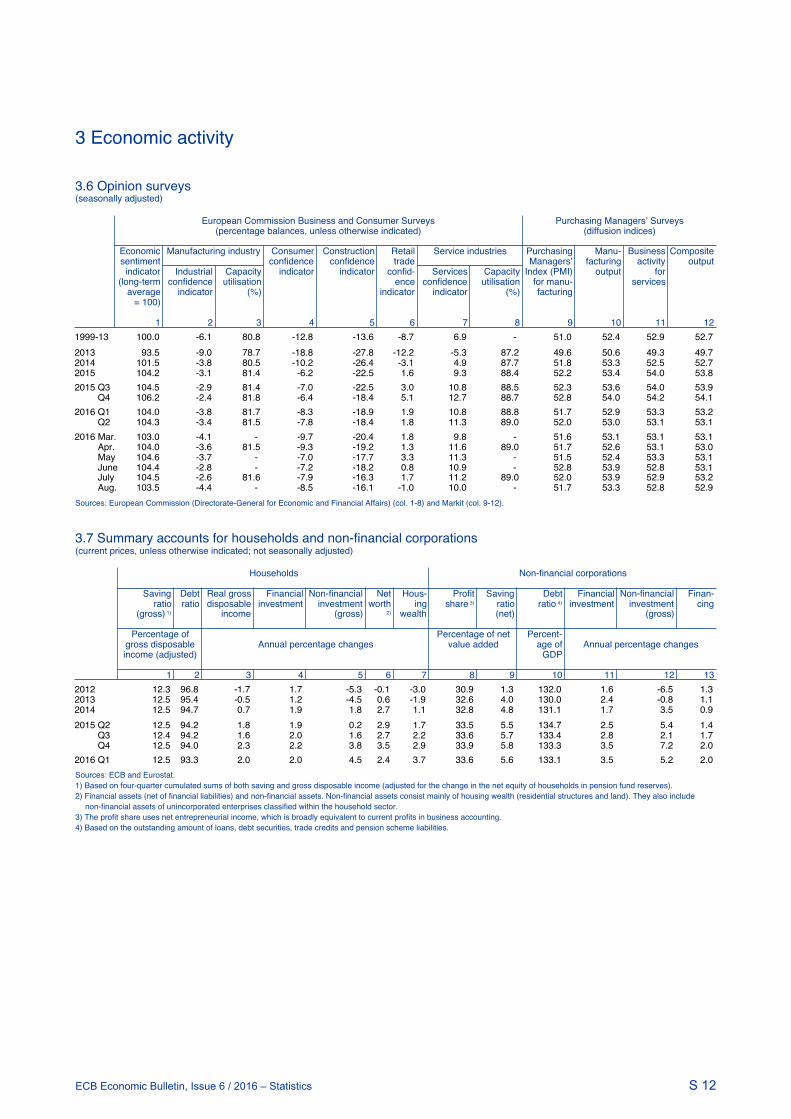
S 12ECB Economic Bulletin, Issue 6 / 2016 – Statistics
3 Economic activity
S 12ECB Economic Bulletin, Issue 6 / 2016 - Statistics
3.6 Opinion surveys(seasonally adjusted)
European Commission Business and Consumer Surveys Purchasing Managersʼ Surveys
(percentage balances, unless otherwise indicated) (diffusion indices)
Economic Manufacturing industry Consumer Construction Retail Service industries Purchasing Manu- Business Compositesentiment confidence confidence trade Managersʼ facturing activity outputindicator Industrial Capacity indicator indicator confid- Services Capacity Index (PMI) output for
(long-term confidence utilisation ence confidence utilisation for manu- servicesaverage indicator (%) indicator indicator (%) facturing
= 100)
1 2 3 4 5 6 7 8 9 10 11 121999-13 100.0 -6.1 80.8 -12.8 -13.6 -8.7 6.9 - 51.0 52.4 52.9 52.72013 93.5 -9.0 78.7 -18.8 -27.8 -12.2 -5.3 87.2 49.6 50.6 49.3 49.72014 101.5 -3.8 80.5 -10.2 -26.4 -3.1 4.9 87.7 51.8 53.3 52.5 52.72015 104.2 -3.1 81.4 -6.2 -22.5 1.6 9.3 88.4 52.2 53.4 54.0 53.82015 Q3 104.5 -2.9 81.4 -7.0 -22.5 3.0 10.8 88.5 52.3 53.6 54.0 53.9 Q4 106.2 -2.4 81.8 -6.4 -18.4 5.1 12.7 88.7 52.8 54.0 54.2 54.12016 Q1 104.0 -3.8 81.7 -8.3 -18.9 1.9 10.8 88.8 51.7 52.9 53.3 53.2 Q2 104.3 -3.4 81.5 -7.8 -18.4 1.8 11.3 89.0 52.0 53.0 53.1 53.12016 Mar. 103.0 -4.1 - -9.7 -20.4 1.8 9.8 - 51.6 53.1 53.1 53.1 Apr. 104.0 -3.6 81.5 -9.3 -19.2 1.3 11.6 89.0 51.7 52.6 53.1 53.0 May 104.6 -3.7 - -7.0 -17.7 3.3 11.3 - 51.5 52.4 53.3 53.1 June 104.4 -2.8 - -7.2 -18.2 0.8 10.9 - 52.8 53.9 52.8 53.1 July 104.5 -2.6 81.6 -7.9 -16.3 1.7 11.2 89.0 52.0 53.9 52.9 53.2 Aug. 103.5 -4.4 - -8.5 -16.1 -1.0 10.0 - 51.7 53.3 52.8 52.9Sources: European Commission (Directorate-General for Economic and Financial Affairs) (col. 1-8) and Markit (col. 9-12).
3.7 Summary accounts for households and non-financial corporations(current prices, unless otherwise indicated; not seasonally adjusted)
Households Non-financial corporations
Saving Debt Real gross Financial Non-financial Net Hous- Profit Saving Debt Financial Non-financial Finan-ratio ratio disposable investment investment worth ing share 3) ratio ratio 4) investment investment cing
(gross) 1) income (gross) 2) wealth (net) (gross)
Percentage of Percentage of net Percent- gross disposable Annual percentage changes value added age of Annual percentage changes income (adjusted) GDP
1 2 3 4 5 6 7 8 9 10 11 12 132012 12.3 96.8 -1.7 1.7 -5.3 -0.1 -3.0 30.9 1.3 132.0 1.6 -6.5 1.32013 12.5 95.4 -0.5 1.2 -4.5 0.6 -1.9 32.6 4.0 130.0 2.4 -0.8 1.12014 12.5 94.7 0.7 1.9 1.8 2.7 1.1 32.8 4.8 131.1 1.7 3.5 0.92015 Q2 12.5 94.2 1.8 1.9 0.2 2.9 1.7 33.5 5.5 134.7 2.5 5.4 1.4 Q3 12.4 94.2 1.6 2.0 1.6 2.7 2.2 33.6 5.7 133.4 2.8 2.1 1.7 Q4 12.5 94.0 2.3 2.2 3.8 3.5 2.9 33.9 5.8 133.3 3.5 7.2 2.02016 Q1 12.5 93.3 2.0 2.0 4.5 2.4 3.7 33.6 5.6 133.1 3.5 5.2 2.0Sources: ECB and Eurostat.1) Based on four-quarter cumulated sums of both saving and gross disposable income (adjusted for the change in the net equity of households in pension fund reserves).2) Financial assets (net of financial liabilities) and non-financial assets. Non-financial assets consist mainly of housing wealth (residential structures and land). They also include
non-financial assets of unincorporated enterprises classified within the household sector.3) The profit share uses net entrepreneurial income, which is broadly equivalent to current profits in business accounting. 4) Based on the outstanding amount of loans, debt securities, trade credits and pension scheme liabilities.

S 13ECB Economic Bulletin, Issue 6 / 2016 – Statistics
3 Economic activity
S 13ECB Economic Bulletin, Issue 6 / 2016 - Statistics
3.8 Euro area balance of payments, current and capital accounts(EUR billions; seasonally adjusted unless otherwise indicated; transactions)
Current account Capital
account 1)
Total Goods Services Primary income Secondary income
Credit Debit Net Credit Debit Credit Debit Credit Debit Credit Debit Credit Debit
1 2 3 4 5 6 7 8 9 10 11 12 132015 Q3 896.3 815.5 80.8 523.9 436.9 191.7 177.8 155.6 144.0 25.1 56.9 9.9 4.6 Q4 898.8 815.7 83.1 525.3 433.5 195.2 182.0 152.5 143.2 25.8 57.1 15.7 9.32016 Q1 881.7 794.3 87.4 516.0 424.0 193.8 176.7 147.5 137.7 24.4 55.9 10.2 11.1 Q2 867.9 771.3 96.5 513.9 416.5 186.9 168.7 141.7 132.0 25.3 54.1 7.3 6.02016 Jan. 294.6 266.0 28.6 172.1 141.9 64.3 59.8 50.3 46.3 8.0 18.1 2.7 4.9 Feb. 293.6 267.2 26.4 170.6 142.1 65.5 59.4 49.4 46.7 8.1 19.0 3.8 2.5 Mar. 293.5 261.1 32.4 173.3 139.9 64.1 57.6 47.8 44.8 8.3 18.8 3.6 3.7 Apr. 293.6 257.1 36.5 172.8 139.4 62.3 55.9 50.0 43.4 8.5 18.4 2.1 1.9 May 289.1 257.3 31.8 170.5 139.4 62.7 56.2 47.1 44.0 8.7 17.6 1.9 1.9 June 285.1 256.9 28.2 170.6 137.6 61.9 56.6 44.6 44.5 8.1 18.2 3.2 2.2
12-month cumulated transactions2016 June 3,544.7 3,196.9 347.8 2,079.2 1,710.8 767.7 705.2 597.2 556.8 100.6 224.0 43.0 31.1
12-month cumulated transactions as a percentage of GDP2016 June 33.5 30.2 3.3 19.6 16.1 7.2 6.7 5.6 5.3 0.9 2.1 0.4 0.31) The capital account is not seasonally adjusted.
3.9 Euro area external trade in goods 1) , values and volumes by product group 2)(seasonally adjusted, unless otherwise indicated)
Values (EUR billions; annual percentage changes for columns 1 and 2)
Total (n.s.a.) Exports (f.o.b.) Imports (c.i.f.)
Total Memo item: Total Memo items:
Exports Imports Intermediate Capital Consump- Manu- Intermediate Capital Consump- Manu- Oilgoods goods tion facturing goods goods tion facturing
goods goods
1 2 3 4 5 6 7 8 9 10 11 12 13
2015 Q3 4.4 0.8 502.5 232.6 104.7 152.9 423.5 444.5 252.4 70.7 112.6 317.7 50.3 Q4 3.6 2.2 509.1 236.7 105.6 153.7 426.3 443.3 246.8 73.1 114.3 324.4 44.62016 Q1 -1.1 -2.6 502.5 233.5 104.0 151.1 422.0 437.4 240.9 71.3 116.4 325.8 37.3 Q2 -0.4 -4.2 501.3 . . . 431.1 428.0 . . . 322.0 . 2016 Jan. -2.1 -0.9 167.4 78.1 34.2 50.6 141.1 147.0 81.5 23.3 38.9 109.6 12.6 Feb. 1.2 2.0 167.0 78.1 34.0 50.3 140.1 147.0 80.4 24.0 39.0 110.0 12.1 Mar. -2.2 -8.1 168.1 77.3 35.8 50.1 140.8 143.4 79.0 23.9 38.5 106.1 12.6 Apr. -0.9 -5.3 168.7 77.7 35.7 51.0 146.1 143.4 78.1 23.9 38.4 109.1 13.3 May 2.0 -2.2 165.8 75.8 34.7 50.6 140.9 141.2 77.9 22.6 38.0 105.7 14.2 June -2.2 -5.0 166.7 . . . 144.1 143.3 . . . 107.2 .
Volume indices (2000 = 100; annual percentage changes for columns 1 and 2)2015 Q3 1.2 2.9 116.2 111.5 118.6 122.6 116.9 105.9 105.3 106.1 106.4 107.9 98.6 Q4 0.9 4.9 118.3 115.2 119.1 122.5 117.4 107.3 107.3 107.2 107.7 110.1 101.32016 Q1 -1.1 2.4 118.4 116.0 117.3 121.7 117.0 109.7 110.8 105.4 109.6 111.1 110.6 Q2 . . . . . . . . . . . . . 2015 Dec. 0.8 4.4 119.0 116.2 118.4 123.6 116.6 107.7 108.3 102.0 109.3 108.9 106.82016 Jan. -3.7 1.2 117.9 115.8 115.6 121.8 116.8 109.8 111.2 104.1 108.9 111.5 110.8 Feb. 1.2 7.0 118.2 116.6 115.2 121.7 116.7 110.7 111.5 106.4 109.8 112.3 114.2 Mar. -0.9 -0.7 119.1 115.7 121.1 121.4 117.5 108.6 109.6 105.8 110.0 109.4 106.7 Apr. 1.4 3.0 119.4 115.5 121.2 124.1 121.9 107.8 106.8 105.9 109.6 112.6 104.7 May 4.9 6.8 117.1 112.6 117.3 122.5 117.5 106.0 105.9 100.2 110.0 109.9 100.9Sources: ECB and Eurostat.1) Differences between ECBʼs b.o.p. goods (Table 3.8) and Eurostatʼs trade in goods (Table 3.9) are mainly due to different definitions.2) Product groups as classified in the Broad Economic Categories.

S 14ECB Economic Bulletin, Issue 6 / 2016 – Statistics
4 Prices and costs
S 14ECB Economic Bulletin, Issue 6 / 2016 - Statistics
4.1 Harmonised Index of Consumer Prices 1)(annual percentage changes, unless otherwise indicated)
Total Total (s.a.; percentage change vis-à-vis previous period) 2) Memo item:
Administered pricesIndex: Total Goods Services Total Processed Unpro- Non-energy Energy Services2015 food cessed industrial (n.s.a.) Total HICP Adminis-
= 100 Total food goods excluding teredexcluding administered pricesfood and prices
energy
1 2 3 4 5 6 7 8 9 10 11 12 13% of total 100.0 100.0 70.7 55.8 44.2 100.0 12.1 7.4 26.5 9.7 44.2 86.5 13.5in 2016 2013 99.5 1.4 1.1 1.3 1.4 - - - - - - 1.2 2.12014 100.0 0.4 0.8 -0.2 1.2 - - - - - - 0.2 1.92015 100.0 0.0 0.8 -0.8 1.2 - - - - - - -0.1 0.92015 Q3 100.0 0.1 0.9 -0.8 1.2 0.0 0.1 0.3 0.2 -2.5 0.3 0.0 0.9 Q4 100.2 0.2 1.0 -0.6 1.2 -0.1 0.1 1.0 0.1 -3.0 0.2 0.1 0.72016 Q1 99.2 0.0 1.0 -0.8 1.1 -0.4 0.1 -0.8 0.1 -4.4 0.2 0.0 0.3 Q2 100.4 -0.1 0.8 -0.9 1.0 0.4 0.2 0.8 0.1 2.0 0.3 -0.1 0.12016 Mar. 100.1 0.0 1.0 -1.1 1.4 0.3 0.0 0.6 0.0 1.0 0.3 -0.1 0.4 Apr. 100.2 -0.2 0.7 -1.1 0.9 0.0 0.2 0.2 0.0 0.1 -0.1 -0.3 0.1 May 100.5 -0.1 0.8 -0.9 1.0 0.3 0.0 0.4 0.0 1.7 0.2 -0.1 0.1 June 100.7 0.1 0.9 -0.7 1.1 0.2 0.1 -0.2 0.0 1.7 0.1 0.1 0.3 July 100.1 0.2 0.9 -0.6 1.2 0.0 0.0 0.9 0.0 -1.0 0.2 0.1 0.4 Aug. 3) 100.2 0.2 0.8 . 1.1 0.0 0.1 0.6 0.0 -1.1 0.0 . .
Goods Services
Food (including alcoholic Industrial goods Housing Transport Communi- Recreation Miscel- beverages and tobacco) cation and laneous
personalTotal Processed Unpro- Total Non-energy Energy Rents
food cessed industrialfood goods
14 15 16 17 18 19 20 21 22 23 24 25% of total 19.5 12.1 7.4 36.3 26.5 9.7 10.7 6.4 7.1 3.2 15.2 8.0in 2016 2013 2.7 2.2 3.5 0.6 0.6 0.6 1.7 1.4 2.4 -4.2 2.3 0.72014 0.5 1.2 -0.8 -0.5 0.1 -1.9 1.7 1.4 1.7 -2.8 1.5 1.32015 1.0 0.6 1.6 -1.8 0.3 -6.8 1.2 1.1 1.3 -0.8 1.5 1.22015 Q3 1.2 0.6 2.1 -1.8 0.4 -7.2 1.1 0.9 1.4 -0.4 1.7 1.0 Q4 1.4 0.7 2.6 -1.7 0.5 -7.2 1.2 1.0 1.1 -0.1 1.5 1.22016 Q1 0.8 0.6 1.1 -1.7 0.6 -7.4 1.1 1.0 0.6 0.0 1.6 1.2 Q2 0.9 0.5 1.4 -1.9 0.5 -7.7 1.1 1.0 0.6 0.0 1.3 1.22016 Mar. 0.8 0.4 1.3 -2.1 0.5 -8.7 1.1 1.0 0.7 0.1 2.1 1.3 Apr. 0.8 0.5 1.2 -2.1 0.5 -8.7 1.1 1.0 0.5 0.1 0.9 1.2 May 0.9 0.6 1.5 -1.9 0.5 -8.1 1.1 1.0 0.5 0.0 1.4 1.1 June 0.9 0.5 1.5 -1.6 0.4 -6.4 1.0 1.0 0.8 -0.1 1.6 1.3 July 1.4 0.5 2.9 -1.7 0.4 -6.7 1.0 1.0 1.0 0.0 1.5 1.4 Aug. 3) 1.3 0.5 2.5 . 0.3 -5.7 . . . . . . Sources: Eurostat and ECB calculations.1) Data refer to the changing composition of the euro area.2) In May 2016 the ECB started publishing enhanced seasonally adjusted HICP series for the euro area, following a review of the seasonal adjustment approach as described
in Box 1, Economic Bulletin, Issue 3, ECB, 2016 (https://www.ecb.europa.eu/pub/pdf/ecbu/eb201603.en.pdf).3) Estimate based on provisional national data, which usually cover around 95% of the euro area, as well as on early information on energy prices.
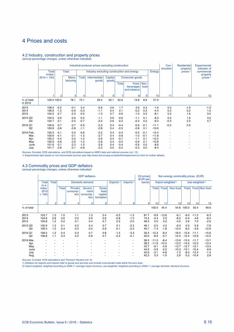
S 15ECB Economic Bulletin, Issue 6 / 2016 – Statistics
4 Prices and costs
S 15ECB Economic Bulletin, Issue 6 / 2016 - Statistics
4.2 Industry, construction and property prices(annual percentage changes, unless otherwise indicated)
Industrial producer prices excluding construction Con- Residential Experimental struction property indicator of
Total Total Industry excluding construction and energy Energy prices 1) commercial(index: property
2010 = 100) Manu- Total Intermediate Capital Consumer goods prices 1)
facturing goods goodsTotal Food, Non-
beverages foodand tobacco
1 2 3 4 5 6 7 8 9 10 11 12 13% of total 100.0 100.0 78.1 72.1 29.4 20.1 22.6 13.8 8.9 27.9 in 2010 2013 108.5 -0.2 -0.1 0.4 -0.6 0.6 1.7 2.6 0.3 -1.6 0.3 -1.9 -1.02014 106.9 -1.5 -0.9 -0.3 -1.1 0.4 0.1 -0.2 0.3 -4.4 0.3 0.2 1.02015 104.0 -2.7 -2.3 -0.5 -1.3 0.7 -0.6 -1.0 0.2 -8.1 0.2 1.6 3.52015 Q3 104.0 -2.6 -2.6 -0.5 -1.1 0.6 -0.6 -1.1 0.1 -8.3 0.3 1.6 3.2 Q4 102.7 -3.1 -2.5 -0.7 -2.0 0.6 -0.2 -0.3 0.2 -9.3 -0.3 2.2 4.72016 Q1 100.6 -3.7 -2.7 -0.9 -2.2 0.4 -0.4 -0.6 -0.1 -11.1 -0.2 2.9 . Q2 100.9 -3.8 -2.8 -1.1 -2.8 0.4 -0.5 -0.8 0.1 -10.6 . . . 2016 Feb. 100.3 -4.1 -3.0 -0.8 -2.2 0.4 -0.4 -0.5 -0.1 -12.4 - - - Mar. 100.6 -4.1 -3.1 -1.2 -2.7 0.4 -0.6 -1.0 -0.1 -11.8 - - - Apr. 100.2 -4.4 -3.2 -1.2 -2.9 0.4 -0.7 -1.1 0.1 -12.5 - - - May 100.9 -3.8 -2.9 -1.2 -2.8 0.4 -0.5 -0.9 0.1 -10.8 - - - June 101.6 -3.1 -2.3 -1.0 -2.6 0.4 -0.4 -0.6 0.0 -8.6 - - - July 101.7 -2.8 -2.1 -0.8 -2.3 0.5 -0.2 -0.3 0.0 -8.4 - - - Sources: Eurostat, ECB calculations, and ECB calculations based on MSCI data and national sources (col. 13).1) Experimental data based on non-harmonised sources (see http://www.ecb.europa.eu/stats/html/experiment.en.html for further details).
4.3 Commodity prices and GDP deflators(annual percentage changes, unless otherwise indicated)
GDP deflators Oil prices Non-energy commodity prices (EUR) (EUR per
Total Total Domestic demand Exports 1) Imports 1) barrel) Import-weighted 2) Use-weighted 2)
(s.a.;index: Total Private Govern- Gross Total Food Non-food Total Food Non-food2010 consump- ment fixed
= 100) tion consump- capitaltion formation
1 2 3 4 5 6 7 8 9 10 11 12 13 14 15% of total 100.0 45.4 54.6 100.0 50.4 49.6
2013 103.7 1.3 1.0 1.1 1.3 0.4 -0.5 -1.3 81.7 -9.9 -13.6 -6.1 -9.0 -11.2 -6.32014 104.6 0.8 0.6 0.5 0.9 0.6 -0.8 -1.5 74.5 -3.4 2.0 -8.5 -0.4 4.6 -6.42015 105.8 1.2 0.2 0.1 0.4 0.7 0.2 -2.0 48.3 0.0 4.2 -4.5 2.9 7.0 -2.62015 Q3 105.9 1.2 0.1 0.2 0.4 0.7 0.1 -2.3 46.1 -2.5 4.2 -9.3 0.0 5.9 -7.8 Q4 106.4 1.3 0.4 0.3 0.5 0.9 -0.1 -2.3 40.7 -7.4 -1.8 -13.4 -8.2 -4.8 -12.92016 Q1 106.5 1.2 0.4 0.3 0.7 0.8 -1.5 -3.3 32.5 -12.3 -8.4 -16.5 -12.9 -11.1 -15.6 Q2 106.8 1.1 0.4 0.2 0.9 0.7 -2.2 -4.1 42.0 -8.9 -5.7 -12.4 -12.4 -12.6 -12.22016 Mar. - - - - - - - - 36.5 -11.0 -8.4 -13.9 -12.5 -11.7 -13.7 Apr. - - - - - - - - 38.2 -11.6 -10.2 -13.2 -14.5 -15.3 -13.4 May - - - - - - - - 42.7 -9.1 -4.9 -13.7 -12.7 -12.1 -13.5 June - - - - - - - - 44.9 -5.9 -2.0 -10.3 -10.1 -10.4 -9.6 July - - - - - - - - 42.6 -3.1 -4.8 -1.2 -8.0 -12.3 -1.4 Aug. - - - - - - - - 42.3 0.3 -1.9 2.9 -5.2 -10.4 2.8Sources: Eurostat, ECB calculations and Thomson Reuters (col. 9).1) Deflators for exports and imports refer to goods and services and include cross-border trade within the euro area.2) Import-weighted: weighted according to 2009-11 average import structure; use-weighted: weighted according to 2009-11 average domestic demand structure.
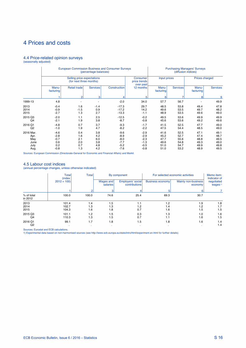
S 16ECB Economic Bulletin, Issue 6 / 2016 – Statistics
4 Prices and costs
S 16ECB Economic Bulletin, Issue 6 / 2016 - Statistics
4.4 Price-related opinion surveys(seasonally adjusted)
European Commission Business and Consumer Surveys Purchasing Managersʼ Surveys
(percentage balances) (diffusion indices)
Selling price expectations Consumer Input prices Prices charged (for next three months) price trends
over pastManu- Retail trade Services Construction 12 months Manu- Services Manu- Services
facturing facturing facturing
1 2 3 4 5 6 7 8 91999-13 4.8 - - -2.0 34.0 57.7 56.7 - 49.92013 -0.4 1.6 -1.4 -17.3 29.7 48.5 53.8 49.4 47.82014 -0.9 -1.5 0.9 -17.2 14.2 49.6 53.5 49.7 48.22015 -2.7 1.3 2.7 -13.3 -1.1 48.9 53.5 49.6 49.02015 Q3 -2.0 1.1 2.5 -12.5 -0.2 49.5 53.6 49.9 49.9 Q4 -2.1 1.9 3.8 -8.7 -0.8 45.6 53.6 49.2 49.62016 Q1 -4.8 0.7 3.7 -9.3 -1.7 41.5 52.5 47.7 49.0 Q2 -1.0 1.9 4.7 -8.2 -2.2 47.5 54.4 48.5 49.02016 Mar. -4.6 0.4 3.8 -9.6 -2.9 41.6 52.5 47.1 49.1 Apr. -2.8 1.6 4.2 -8.9 -2.9 45.2 52.7 47.4 48.7 May -0.7 2.1 6.0 -8.0 -2.3 47.7 55.6 48.8 49.5 June 0.6 2.0 3.8 -7.7 -1.3 49.6 54.8 49.3 49.0 July 0.2 0.7 4.8 -5.2 -0.5 51.0 54.7 49.9 49.8 Aug. -0.8 1.3 4.2 -7.6 -0.8 51.0 53.2 48.9 49.5Sources: European Commission (Directorate-General for Economic and Financial Affairs) and Markit.
4.5 Labour cost indices(annual percentage changes, unless otherwise indicated)
Total Total By component For selected economic activities Memo item:
(index: Indicator of2012 = 100) Wages and Employersʼ social Business economy Mainly non-business negotiated
salaries contributions economy wages 1)
1 2 3 4 5 6 7% of total 100.0 100.0 74.6 25.4 69.3 30.7 in 2012 2013 101.4 1.4 1.5 1.1 1.2 1.9 1.82014 102.7 1.3 1.3 1.2 1.4 1.2 1.72015 104.3 1.6 1.8 0.7 1.6 1.5 1.52015 Q3 101.1 1.2 1.5 0.3 1.3 1.0 1.6 Q4 110.3 1.3 1.5 0.7 1.1 1.6 1.52016 Q1 99.1 1.7 1.8 1.5 1.8 1.6 1.4 Q2 . . . . . . 1.4Sources: Eurostat and ECB calculations.1) Experimental data based on non-harmonised sources (see http://www.ecb.europa.eu/stats/intro/html/experiment.en.html for further details).

S 17ECB Economic Bulletin, Issue 6 / 2016 – Statistics
4 Prices and costs
S 17ECB Economic Bulletin, Issue 6 / 2016 - Statistics
4.6 Unit labour costs, compensation per labour input and labour productivity(annual percentage changes, unless otherwise indicated; quarterly data seasonally adjusted; annual data unadjusted)
Unit labour costs
Total Total By economic activity(index:
2010 Agriculture, Manu- Con- Trade, Information Finance Real Professional, Public ad- Arts, enter-=100) forestry facturing, struction transport, and commu- and estate business and ministration, tainment
and fishing energy and accom- nication insurance support education, and otherutilities modation and services health and services
food services social work
1 2 3 4 5 6 7 8 9 10 11 12
2013 103.8 1.2 -2.2 2.2 0.9 0.6 -0.4 0.7 -2.8 1.4 1.7 2.82014 104.6 0.8 -0.8 -0.1 0.6 0.4 -0.3 1.9 1.1 1.7 1.4 0.82015 104.9 0.3 0.9 -1.7 0.5 0.6 0.6 0.4 3.5 1.8 0.9 1.22015 Q2 104.8 0.4 1.3 -1.0 1.1 0.2 0.9 0.1 3.3 1.3 0.8 1.5 Q3 105.0 0.4 1.4 -1.8 0.5 0.7 1.2 0.9 3.7 2.1 0.9 1.3 Q4 105.4 0.6 0.9 -1.8 -0.4 1.6 1.7 0.9 4.0 1.8 1.2 1.22016 Q1 105.4 0.9 1.6 0.6 -0.3 1.1 0.1 1.6 2.5 1.8 1.2 1.1
Compensation per employee 2013 105.2 1.6 2.5 2.6 1.3 0.9 0.8 1.7 0.1 1.3 1.6 1.92014 106.5 1.3 0.1 2.1 1.6 1.0 2.0 1.6 1.1 1.4 1.1 0.62015 107.9 1.3 0.9 1.7 1.0 1.4 2.4 0.7 2.9 1.6 1.1 1.32015 Q2 107.8 1.4 0.4 2.1 0.8 1.5 2.8 0.6 2.1 1.4 1.0 1.5 Q3 108.1 1.3 0.5 1.5 1.3 1.4 2.5 0.6 2.9 1.8 1.0 1.5 Q4 108.5 1.3 1.8 1.3 1.1 1.8 2.1 0.7 3.8 1.4 1.3 1.12016 Q1 108.8 1.2 1.7 1.3 1.6 1.4 -0.1 1.9 1.5 1.5 1.2 1.0
Labour productivity per person employed2013 101.4 0.4 4.8 0.4 0.4 0.3 1.2 1.1 2.9 -0.1 -0.1 -0.82014 101.9 0.5 0.8 2.2 1.0 0.6 2.3 -0.3 0.0 -0.3 -0.3 -0.22015 102.9 1.0 0.1 3.5 0.5 0.8 1.8 0.2 -0.5 -0.2 0.2 0.12015 Q2 102.8 1.0 -0.9 3.1 -0.3 1.3 1.9 0.5 -1.1 0.1 0.2 0.0 Q3 102.9 0.9 -0.9 3.4 0.8 0.7 1.2 -0.3 -0.7 -0.3 0.1 0.2 Q4 103.0 0.7 0.9 3.1 1.5 0.2 0.4 -0.1 -0.2 -0.4 0.0 -0.12016 Q1 103.2 0.3 0.1 0.7 1.9 0.4 -0.2 0.2 -0.9 -0.4 0.1 -0.1
Compensation per hour worked 2013 107.2 2.3 2.3 2.8 2.8 1.9 0.9 2.3 1.5 2.5 2.0 3.22014 108.5 1.2 1.3 1.6 1.4 1.1 1.8 1.6 0.8 1.2 0.8 1.32015 109.6 1.0 0.4 1.2 0.3 1.4 1.2 0.9 2.5 1.3 0.9 1.02015 Q2 109.4 1.1 0.0 1.4 0.3 1.6 1.5 0.7 1.1 1.1 0.8 1.5 Q3 109.6 1.0 0.1 0.9 0.6 1.5 1.2 1.0 2.4 1.4 0.7 1.0 Q4 110.0 1.0 0.7 0.4 0.3 1.6 1.2 0.6 3.9 1.1 1.4 1.02016 Q1 110.4 1.1 0.0 1.1 1.5 1.2 -0.5 1.6 1.7 0.7 1.4 1.9
Hourly labour productivity2013 103.5 1.2 4.5 0.6 2.0 1.1 1.6 1.6 4.3 1.1 0.5 0.52014 104.0 0.5 2.3 1.8 0.9 0.8 2.2 -0.2 0.4 -0.3 -0.5 0.42015 104.8 0.8 -0.8 3.0 -0.2 1.0 0.8 0.2 -0.9 -0.4 0.0 -0.12015 Q2 104.8 0.8 -1.3 2.4 -0.8 1.7 0.8 0.6 -1.6 -0.2 0.1 0.0 Q3 104.7 0.6 -1.6 2.8 0.1 1.0 -0.2 -0.1 -1.9 -0.9 -0.2 -0.1 Q4 104.7 0.4 -0.4 2.3 0.4 0.2 -0.3 -0.6 0.2 -0.5 0.1 -0.22016 Q1 105.0 0.1 -1.5 0.5 1.2 0.2 -0.7 -0.1 -0.5 -1.0 0.2 0.8Sources: Eurostat and ECB calculations.

S 18ECB Economic Bulletin, Issue 6 / 2016 – Statistics
5 Money and credit
S 18ECB Economic Bulletin, Issue 6 / 2016 - Statistics
5.1 Monetary aggregates 1)(EUR billions and annual growth rates; seasonally adjusted; outstanding amounts and growth rates at end of period; transactions during period)
Outstanding amounts
M3
M2 M3-M2
M1 M2-M1
Currency Overnight Deposits Deposits Repos Money Debtin deposits with an redeemable market securities
circulation agreed at notice fund withmaturity of up to shares a maturityof up to 3 months of up to2 years 2 years
1 2 3 4 5 6 7 8 9 10 11 12
2013 909.7 4,476.3 5,386.1 1,683.3 2,142.8 3,826.1 9,212.1 121.4 418.1 86.5 626.0 9,838.12014 968.5 4,981.3 5,949.9 1,598.5 2,148.8 3,747.2 9,697.1 123.9 423.4 106.2 653.4 10,350.52015 1,034.5 5,569.7 6,604.1 1,448.1 2,160.6 3,608.7 10,212.8 77.1 474.2 72.9 624.3 10,837.12015 Q3 1,028.2 5,434.8 6,463.0 1,449.3 2,164.4 3,613.7 10,076.7 98.4 452.8 75.0 626.2 10,703.0 Q4 1,034.5 5,569.7 6,604.1 1,448.1 2,160.6 3,608.7 10,212.8 77.1 474.2 72.9 624.3 10,837.12016 Q1 1,051.5 5,715.1 6,766.6 1,426.9 2,163.7 3,590.6 10,357.2 88.7 463.3 89.9 642.0 10,999.1 Q2 1,053.4 5,812.9 6,866.3 1,417.3 2,173.6 3,591.0 10,457.2 83.3 481.5 92.7 657.6 11,114.82016 Feb. 1,046.9 5,669.4 6,716.2 1,430.2 2,165.1 3,595.2 10,311.4 92.6 468.1 88.9 649.5 10,960.9 Mar. 1,051.5 5,715.1 6,766.6 1,426.9 2,163.7 3,590.6 10,357.2 88.7 463.3 89.9 642.0 10,999.1 Apr. 1,047.5 5,747.8 6,795.4 1,408.6 2,162.6 3,571.2 10,366.6 88.4 470.4 98.4 657.2 11,023.7 May 1,051.2 5,789.7 6,840.9 1,407.5 2,172.2 3,579.7 10,420.6 88.3 474.7 88.6 651.5 11,072.1 June 1,053.4 5,812.9 6,866.3 1,417.3 2,173.6 3,591.0 10,457.2 83.3 481.5 92.7 657.6 11,114.8 July (p) 1,056.2 5,869.8 6,926.0 1,406.7 2,174.6 3,581.3 10,507.3 82.4 486.6 98.1 667.1 11,174.4
Transactions2013 45.6 250.4 295.9 -114.4 45.5 -68.9 227.0 -11.6 -48.7 -63.3 -123.6 103.42014 58.2 379.4 437.5 -90.9 3.2 -87.7 349.8 1.0 10.8 12.5 24.4 374.22015 64.8 556.1 620.9 -143.2 12.0 -131.2 489.7 -47.8 48.9 -26.0 -24.9 464.82015 Q3 14.3 130.7 145.0 -35.3 3.1 -32.3 112.7 10.2 18.3 -18.5 10.0 122.7 Q4 6.3 128.1 134.4 -3.4 -4.0 -7.4 127.0 -21.5 21.4 -2.5 -2.6 124.42016 Q1 17.2 155.9 173.1 -17.0 3.3 -13.7 159.4 12.1 -10.9 14.9 16.1 175.4 Q2 1.8 92.9 94.7 -12.2 10.1 -2.1 92.6 -2.5 17.7 1.6 16.8 109.32016 Feb. 2.4 43.1 45.5 -18.2 8.3 -10.0 35.5 6.4 -6.1 9.1 9.5 45.0 Mar. 4.7 55.2 59.9 -1.2 -1.3 -2.5 57.4 -3.4 -5.4 1.3 -7.5 49.9 Apr. -4.0 31.7 27.7 -18.5 -1.0 -19.5 8.2 2.8 6.8 8.7 18.4 26.6 May 3.7 37.3 40.9 -2.9 9.5 6.6 47.6 -0.3 4.3 -9.4 -5.3 42.2 June 2.2 23.9 26.1 9.1 1.6 10.8 36.8 -5.0 6.5 2.2 3.7 40.6 July (p) 2.9 56.3 59.2 -9.9 1.0 -9.0 50.2 -0.9 5.1 4.9 9.1 59.3
Growth rates2013 5.3 5.9 5.8 -6.4 2.2 -1.8 2.5 -9.2 -10.4 -38.0 -16.1 1.02014 6.4 8.4 8.1 -5.4 0.1 -2.3 3.8 0.8 2.6 18.4 3.9 3.82015 6.7 11.1 10.4 -9.0 0.6 -3.5 5.0 -38.3 11.5 -25.4 -3.8 4.52015 Q3 8.3 11.9 11.3 -11.4 0.5 -4.7 5.0 -23.0 9.0 -1.0 0.6 4.7 Q4 6.7 11.1 10.4 -9.0 0.6 -3.5 5.0 -38.3 11.5 -25.4 -3.8 4.52016 Q1 5.9 11.0 10.2 -6.8 0.6 -2.4 5.5 -27.8 7.6 -1.9 -0.6 5.1 Q2 3.9 9.6 8.7 -4.6 0.6 -1.5 4.9 -2.1 10.7 -4.0 6.5 5.02016 Feb. 5.7 11.1 10.2 -7.4 0.9 -2.6 5.4 -27.1 7.6 -10.2 -1.8 5.0 Mar. 5.9 11.0 10.2 -6.8 0.6 -2.4 5.5 -27.8 7.6 -1.9 -0.6 5.1 Apr. 4.6 10.7 9.7 -7.3 0.4 -2.8 5.1 -27.3 6.1 -4.0 -1.8 4.6 May 4.5 10.0 9.1 -5.8 0.7 -2.0 5.1 -15.1 8.5 -1.8 3.0 4.9 June 3.9 9.6 8.7 -4.6 0.6 -1.5 4.9 -2.1 10.7 -4.0 6.5 5.0 July (p) 3.5 9.3 8.4 -4.4 0.6 -1.4 4.8 -16.9 8.1 14.8 4.9 4.8Source: ECB.1) Data refer to the changing composition of the euro area.
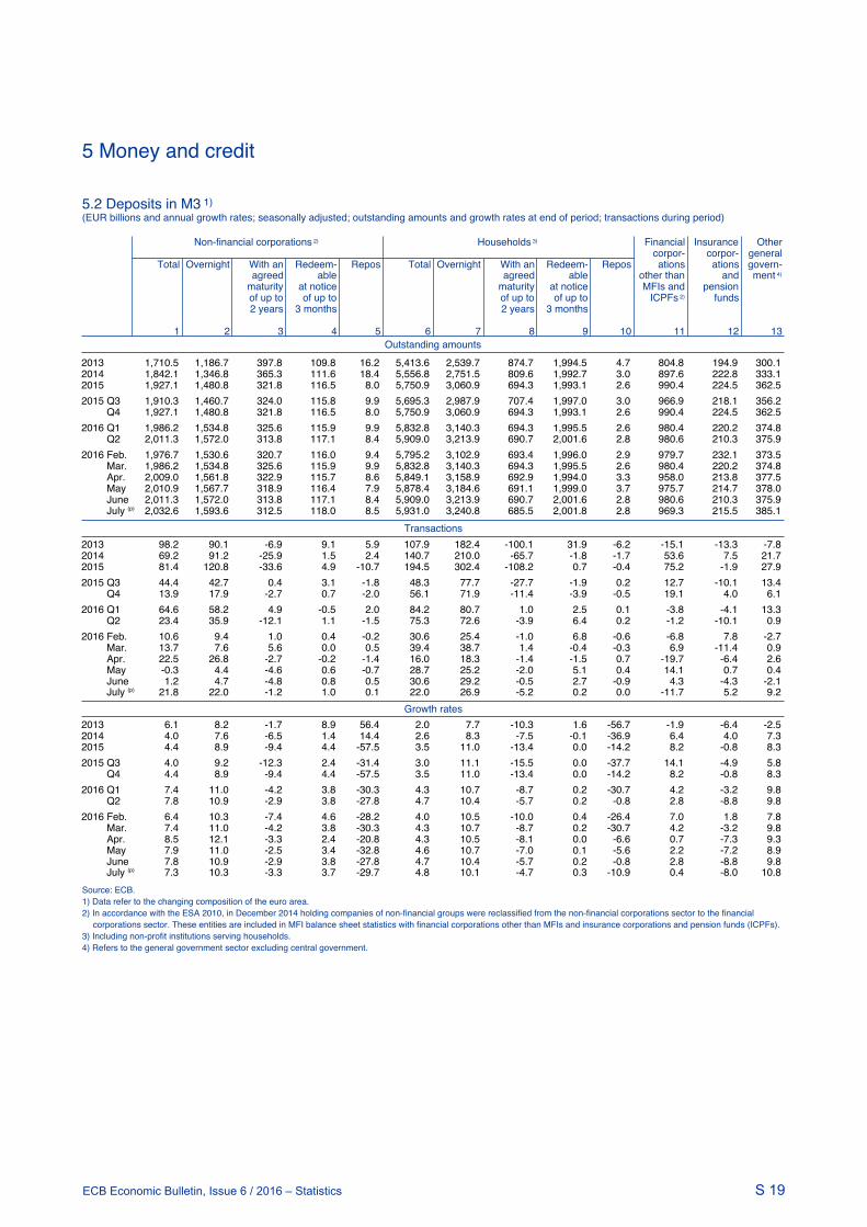
S 19ECB Economic Bulletin, Issue 6 / 2016 – Statistics
5 Money and credit
S 19ECB Economic Bulletin, Issue 6 / 2016 - Statistics
5.2 Deposits in M3 1)(EUR billions and annual growth rates; seasonally adjusted; outstanding amounts and growth rates at end of period; transactions during period)
Outstanding amounts
Non-financial corporations 2) Households 3) Financial Insurance Other
corpor- corpor- generalTotal Overnight With an Redeem- Repos Total Overnight With an Redeem- Repos ations ations govern-
agreed able agreed able other than and ment 4)
maturity at notice maturity at notice MFIs and pensionof up to of up to of up to of up to ICPFs 2) funds2 years 3 months 2 years 3 months
1 2 3 4 5 6 7 8 9 10 11 12 13
2013 1,710.5 1,186.7 397.8 109.8 16.2 5,413.6 2,539.7 874.7 1,994.5 4.7 804.8 194.9 300.12014 1,842.1 1,346.8 365.3 111.6 18.4 5,556.8 2,751.5 809.6 1,992.7 3.0 897.6 222.8 333.12015 1,927.1 1,480.8 321.8 116.5 8.0 5,750.9 3,060.9 694.3 1,993.1 2.6 990.4 224.5 362.52015 Q3 1,910.3 1,460.7 324.0 115.8 9.9 5,695.3 2,987.9 707.4 1,997.0 3.0 966.9 218.1 356.2 Q4 1,927.1 1,480.8 321.8 116.5 8.0 5,750.9 3,060.9 694.3 1,993.1 2.6 990.4 224.5 362.52016 Q1 1,986.2 1,534.8 325.6 115.9 9.9 5,832.8 3,140.3 694.3 1,995.5 2.6 980.4 220.2 374.8 Q2 2,011.3 1,572.0 313.8 117.1 8.4 5,909.0 3,213.9 690.7 2,001.6 2.8 980.6 210.3 375.92016 Feb. 1,976.7 1,530.6 320.7 116.0 9.4 5,795.2 3,102.9 693.4 1,996.0 2.9 979.7 232.1 373.5 Mar. 1,986.2 1,534.8 325.6 115.9 9.9 5,832.8 3,140.3 694.3 1,995.5 2.6 980.4 220.2 374.8 Apr. 2,009.0 1,561.8 322.9 115.7 8.6 5,849.1 3,158.9 692.9 1,994.0 3.3 958.0 213.8 377.5 May 2,010.9 1,567.7 318.9 116.4 7.9 5,878.4 3,184.6 691.1 1,999.0 3.7 975.7 214.7 378.0 June 2,011.3 1,572.0 313.8 117.1 8.4 5,909.0 3,213.9 690.7 2,001.6 2.8 980.6 210.3 375.9 July (p) 2,032.6 1,593.6 312.5 118.0 8.5 5,931.0 3,240.8 685.5 2,001.8 2.8 969.3 215.5 385.1
Transactions2013 98.2 90.1 -6.9 9.1 5.9 107.9 182.4 -100.1 31.9 -6.2 -15.1 -13.3 -7.82014 69.2 91.2 -25.9 1.5 2.4 140.7 210.0 -65.7 -1.8 -1.7 53.6 7.5 21.72015 81.4 120.8 -33.6 4.9 -10.7 194.5 302.4 -108.2 0.7 -0.4 75.2 -1.9 27.92015 Q3 44.4 42.7 0.4 3.1 -1.8 48.3 77.7 -27.7 -1.9 0.2 12.7 -10.1 13.4 Q4 13.9 17.9 -2.7 0.7 -2.0 56.1 71.9 -11.4 -3.9 -0.5 19.1 4.0 6.12016 Q1 64.6 58.2 4.9 -0.5 2.0 84.2 80.7 1.0 2.5 0.1 -3.8 -4.1 13.3 Q2 23.4 35.9 -12.1 1.1 -1.5 75.3 72.6 -3.9 6.4 0.2 -1.2 -10.1 0.92016 Feb. 10.6 9.4 1.0 0.4 -0.2 30.6 25.4 -1.0 6.8 -0.6 -6.8 7.8 -2.7 Mar. 13.7 7.6 5.6 0.0 0.5 39.4 38.7 1.4 -0.4 -0.3 6.9 -11.4 0.9 Apr. 22.5 26.8 -2.7 -0.2 -1.4 16.0 18.3 -1.4 -1.5 0.7 -19.7 -6.4 2.6 May -0.3 4.4 -4.6 0.6 -0.7 28.7 25.2 -2.0 5.1 0.4 14.1 0.7 0.4 June 1.2 4.7 -4.8 0.8 0.5 30.6 29.2 -0.5 2.7 -0.9 4.3 -4.3 -2.1 July (p) 21.8 22.0 -1.2 1.0 0.1 22.0 26.9 -5.2 0.2 0.0 -11.7 5.2 9.2
Growth rates2013 6.1 8.2 -1.7 8.9 56.4 2.0 7.7 -10.3 1.6 -56.7 -1.9 -6.4 -2.52014 4.0 7.6 -6.5 1.4 14.4 2.6 8.3 -7.5 -0.1 -36.9 6.4 4.0 7.32015 4.4 8.9 -9.4 4.4 -57.5 3.5 11.0 -13.4 0.0 -14.2 8.2 -0.8 8.32015 Q3 4.0 9.2 -12.3 2.4 -31.4 3.0 11.1 -15.5 0.0 -37.7 14.1 -4.9 5.8 Q4 4.4 8.9 -9.4 4.4 -57.5 3.5 11.0 -13.4 0.0 -14.2 8.2 -0.8 8.32016 Q1 7.4 11.0 -4.2 3.8 -30.3 4.3 10.7 -8.7 0.2 -30.7 4.2 -3.2 9.8 Q2 7.8 10.9 -2.9 3.8 -27.8 4.7 10.4 -5.7 0.2 -0.8 2.8 -8.8 9.82016 Feb. 6.4 10.3 -7.4 4.6 -28.2 4.0 10.5 -10.0 0.4 -26.4 7.0 1.8 7.8 Mar. 7.4 11.0 -4.2 3.8 -30.3 4.3 10.7 -8.7 0.2 -30.7 4.2 -3.2 9.8 Apr. 8.5 12.1 -3.3 2.4 -20.8 4.3 10.5 -8.1 0.0 -6.6 0.7 -7.3 9.3 May 7.9 11.0 -2.5 3.4 -32.8 4.6 10.7 -7.0 0.1 -5.6 2.2 -7.2 8.9 June 7.8 10.9 -2.9 3.8 -27.8 4.7 10.4 -5.7 0.2 -0.8 2.8 -8.8 9.8 July (p) 7.3 10.3 -3.3 3.7 -29.7 4.8 10.1 -4.7 0.3 -10.9 0.4 -8.0 10.8Source: ECB.1) Data refer to the changing composition of the euro area.2) In accordance with the ESA 2010, in December 2014 holding companies of non-financial groups were reclassified from the non-financial corporations sector to the financial
corporations sector. These entities are included in MFI balance sheet statistics with financial corporations other than MFIs and insurance corporations and pension funds (ICPFs).3) Including non-profit institutions serving households.4) Refers to the general government sector excluding central government.
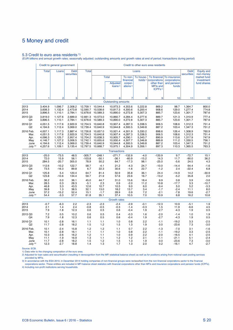
S 20ECB Economic Bulletin, Issue 6 / 2016 – Statistics
5 Money and credit
S 20ECB Economic Bulletin, Issue 6 / 2016 - Statistics
5.3 Credit to euro area residents 1)(EUR billions and annual growth rates; seasonally adjusted; outstanding amounts and growth rates at end of period; transactions during period)
Outstanding amounts
Credit to general government Credit to other euro area residents
Total Loans Debt Total Loans Debt Equity andsecurities securities non-money
Total To non- To house- To financial To insurance market fundfinancial holds 4) corporations corporations investment
Adjusted corpor- other than and pension fund sharesloans 2) ations 3) MFIs and funds
ICPFs 3)
1 2 3 4 5 6 7 8 9 10 11 12
2013 3,404.9 1,096.7 2,308.2 12,709.1 10,544.4 10,973.3 4,353.6 5,222.8 869.2 98.7 1,364.7 800.02014 3,608.3 1,132.4 2,473.8 12,590.7 10,538.6 10,817.3 4,300.6 5,200.4 908.6 129.0 1,277.4 774.82015 3,896.5 1,110.1 2,784.1 12,678.6 10,589.3 10,890.0 4,272.8 5,307.3 885.7 123.6 1,301.7 787.62015 Q3 3,819.0 1,127.6 2,689.0 12,661.3 10,573.0 10,860.7 4,284.4 5,277.6 889.7 121.3 1,310.9 777.4 Q4 3,896.5 1,110.1 2,784.1 12,678.6 10,589.3 10,890.0 4,272.8 5,307.3 885.7 123.6 1,301.7 787.62016 Q1 4,051.5 1,117.6 2,920.9 12,704.5 10,640.8 10,907.4 4,287.3 5,338.5 906.5 108.6 1,312.3 751.4 Q2 4,194.6 1,112.4 3,069.0 12,739.4 10,640.9 10,944.8 4,300.5 5,349.8 887.2 103.4 1,347.3 751.22016 Feb. 4,007.1 1,117.3 2,887.4 12,726.8 10,657.0 10,921.4 4,301.9 5,330.2 898.6 126.4 1,308.9 760.9 Mar. 4,051.5 1,117.6 2,920.9 12,704.5 10,640.8 10,907.4 4,287.3 5,338.5 906.5 108.6 1,312.3 751.4 Apr. 4,096.3 1,125.7 2,957.4 12,704.2 10,638.3 10,905.7 4,290.1 5,343.7 890.9 113.6 1,317.9 747.9 May 4,146.7 1,127.2 3,006.5 12,742.1 10,655.6 10,930.4 4,307.7 5,346.8 889.8 111.2 1,330.5 756.1 June 4,194.6 1,112.4 3,069.0 12,739.4 10,640.9 10,944.8 4,300.5 5,349.8 887.2 103.4 1,347.3 751.2 July (p) 4,257.6 1,109.1 3,135.4 12,797.5 10,668.7 10,975.1 4,304.9 5,356.1 897.3 110.3 1,365.5 763.3
Transactions2013 -25.0 -73.5 48.5 -305.7 -248.1 -271.7 -132.9 -4.0 -120.9 9.7 -72.7 15.12014 72.0 15.9 56.1 -103.8 -50.1 -36.1 -60.9 -15.2 14.3 11.7 -90.0 36.22015 284.5 -20.7 305.0 78.9 50.2 64.7 -17.3 98.1 -25.0 -5.6 24.5 4.32015 Q3 112.6 -10.2 122.7 58.7 -4.1 21.2 -4.3 24.7 -10.0 -14.4 64.4 -1.6 Q4 73.5 -16.3 89.8 6.7 22.3 30.6 -1.6 22.7 -1.2 2.4 -22.4 6.82016 Q1 125.8 5.4 120.4 64.7 81.4 50.9 35.8 36.1 24.4 -14.9 14.2 -30.9 Q2 123.8 -10.6 134.4 59.7 21.9 57.6 23.6 16.7 -13.2 -5.2 35.8 2.02016 Feb. 36.2 0.0 36.1 45.0 44.7 31.0 15.6 18.4 9.9 0.8 3.9 -3.6 Mar. 28.5 0.3 28.3 -5.1 2.3 0.9 -2.0 11.2 10.8 -17.7 3.3 -10.7 Apr. 46.8 3.3 43.5 12.6 10.7 10.5 9.0 6.0 -9.4 5.0 5.2 -3.3 May 39.8 1.3 38.5 32.1 13.0 18.2 13.7 3.4 -1.7 -2.4 11.1 8.0 June 37.2 -15.2 52.4 15.1 -1.7 28.9 0.9 7.2 -2.1 -7.8 19.6 -2.7 July (p) 54.4 -3.3 57.7 61.8 35.1 37.4 10.5 7.0 10.9 6.8 16.2 10.6
Growth rates2013 -0.7 -6.3 2.2 -2.3 -2.3 -2.4 -2.9 -0.1 -12.3 10.9 -5.1 1.92014 2.1 1.4 2.4 -0.8 -0.5 -0.3 -1.4 -0.3 1.5 11.9 -6.6 4.52015 7.9 -1.8 12.3 0.6 0.5 0.6 -0.4 1.9 -2.7 -4.3 1.9 0.52015 Q3 7.2 0.5 10.2 0.6 0.5 0.4 -0.3 1.6 -2.0 -1.4 1.0 1.9 Q4 7.9 -1.8 12.3 0.6 0.5 0.6 -0.4 1.9 -2.7 -4.3 1.9 0.52016 Q1 10.1 -2.8 16.1 1.1 1.1 1.0 0.8 2.2 -1.1 -19.2 3.3 -2.5 Q2 11.7 -2.8 18.2 1.5 1.2 1.5 1.3 1.9 0.0 -23.6 7.3 -3.02016 Feb. 10.1 -2.4 15.8 1.2 1.2 1.1 0.7 2.2 -1.3 -7.0 3.1 -1.6 Mar. 10.1 -2.8 16.1 1.1 1.1 1.0 0.8 2.2 -1.1 -19.2 3.3 -2.5 Apr. 10.3 -2.6 16.2 1.2 1.1 1.0 0.9 2.2 -2.0 -16.5 4.1 -2.5 May 11.1 -1.9 16.9 1.3 1.1 1.2 1.2 2.1 -1.1 -21.1 5.1 -2.4 June 11.7 -2.8 18.2 1.5 1.2 1.5 1.3 1.9 0.0 -23.6 7.3 -3.0 July (p) 12.3 -2.7 18.8 1.4 1.3 1.7 1.3 2.0 0.2 -16.1 4.7 -2.7Source: ECB.1) Data refer to the changing composition of the euro area.2) Adjusted for loan sales and securitisation (resulting in derecognition from the MFI statistical balance sheet) as well as for positions arising from notional cash pooling services
provided by MFIs.3) In accordance with the ESA 2010, in December 2014 holding companies of non-financial groups were reclassified from the non-financial corporations sector to the financial
corporations sector. These entities are included in MFI balance sheet statistics with financial corporations other than MFIs and insurance corporations and pension funds (ICPFs).4) Including non-profit institutions serving households.

S 21ECB Economic Bulletin, Issue 6 / 2016 – Statistics
5 Money and credit
S 21ECB Economic Bulletin, Issue 6 / 2016 - Statistics
5.4 MFI loans to euro area non-financial corporations and households 1)(EUR billions and annual growth rates; seasonally adjusted; outstanding amounts and growth rates at end of period; transactions during period)
Outstanding amounts
Non-financial corporations 2) Households 3)
Total Up to 1 year Over 1 Over 5 years Total Loans for Loans for Other loans
and up to consumption houseAdjusted 5 years Adjusted purchase
loans 4) loans 4)
1 2 3 4 5 6 7 8 9 10
2013 4,353.6 4,450.2 1,065.7 740.9 2,547.0 5,222.8 5,547.8 573.6 3,853.7 795.52014 4,300.6 4,255.9 1,109.9 720.6 2,470.2 5,200.4 5,546.2 563.3 3,861.1 776.02015 4,272.8 4,256.8 1,038.1 758.3 2,476.4 5,307.3 5,640.8 595.6 3,948.0 763.62015 Q3 4,284.4 4,251.9 1,067.7 745.9 2,470.7 5,277.6 5,611.7 582.4 3,926.5 768.7 Q4 4,272.8 4,256.8 1,038.1 758.3 2,476.4 5,307.3 5,640.8 595.6 3,948.0 763.62016 Q1 4,287.3 4,262.0 1,044.6 768.2 2,474.5 5,338.5 5,658.6 603.4 3,972.9 762.2 Q2 4,300.5 4,279.9 1,041.8 774.4 2,484.3 5,349.8 5,684.2 604.2 3,987.0 758.62016 Feb. 4,301.9 4,272.8 1,049.5 774.5 2,477.9 5,330.2 5,652.5 601.4 3,966.8 761.9 Mar. 4,287.3 4,262.0 1,044.6 768.2 2,474.5 5,338.5 5,658.6 603.4 3,972.9 762.2 Apr. 4,290.1 4,264.4 1,043.5 772.7 2,473.9 5,343.7 5,665.2 604.6 3,979.9 759.2 May 4,307.7 4,279.9 1,051.4 771.7 2,484.7 5,346.8 5,673.0 601.8 3,986.1 758.9 June 4,300.5 4,279.9 1,041.8 774.4 2,484.3 5,349.8 5,684.2 604.2 3,987.0 758.6 July (p) 4,304.9 4,286.6 1,034.4 780.7 2,489.8 5,356.1 5,691.9 604.4 3,995.2 756.5
Transactions2013 -132.9 -145.5 -44.3 -44.6 -44.0 -4.0 -17.0 -18.2 27.4 -13.22014 -60.9 -68.3 -14.2 2.3 -49.0 -15.2 5.5 -3.0 -3.4 -8.82015 -17.3 16.7 -65.6 32.7 15.6 98.1 76.3 21.7 80.0 -3.62015 Q3 -4.3 3.2 -17.5 4.0 9.2 24.7 24.8 5.2 19.8 -0.3 Q4 -1.6 15.9 -22.8 13.5 7.7 22.7 19.2 5.1 20.0 -2.42016 Q1 35.8 28.7 15.3 13.0 7.4 36.1 22.8 9.1 27.0 0.1 Q2 23.6 25.2 1.3 8.4 13.9 16.7 31.2 1.0 16.1 -0.42016 Feb. 15.6 16.7 1.7 10.5 3.5 18.4 8.3 5.1 13.3 0.0 Mar. -2.0 -1.7 0.2 -3.8 1.5 11.2 8.1 2.7 7.4 1.0 Apr. 9.0 7.9 1.0 5.0 3.0 6.0 7.0 1.1 7.1 -2.1 May 13.7 9.8 5.9 -0.8 8.6 3.4 7.8 -3.1 6.4 0.1 June 0.9 7.6 -5.6 4.3 2.3 7.2 16.4 3.0 2.6 1.6 July (p) 10.5 11.8 -4.4 7.8 7.0 7.0 9.0 0.2 8.4 -1.6
Growth rates2013 -2.9 -3.2 -4.0 -5.6 -1.7 -0.1 -0.3 -3.0 0.7 -1.62014 -1.4 -1.5 -1.3 0.3 -1.9 -0.3 0.1 -0.5 -0.1 -1.12015 -0.4 0.4 -5.9 4.5 0.6 1.9 1.4 3.8 2.1 -0.52015 Q3 -0.3 0.0 -4.4 3.6 0.3 1.6 1.1 2.6 1.8 -0.4 Q4 -0.4 0.4 -5.9 4.5 0.6 1.9 1.4 3.8 2.1 -0.52016 Q1 0.8 1.1 -2.4 5.2 0.8 2.2 1.6 5.0 2.3 -0.4 Q2 1.3 1.7 -2.2 5.3 1.6 1.9 1.8 3.5 2.1 -0.42016 Feb. 0.7 1.3 -3.0 6.2 0.7 2.2 1.5 5.0 2.3 -0.3 Mar. 0.8 1.1 -2.4 5.2 0.8 2.2 1.6 5.0 2.3 -0.4 Apr. 0.9 1.3 -2.6 5.7 1.1 2.2 1.5 5.3 2.3 -0.7 May 1.2 1.6 -2.0 4.9 1.4 2.1 1.6 4.5 2.3 -0.7 June 1.3 1.7 -2.2 5.3 1.6 1.9 1.8 3.5 2.1 -0.4 July (p) 1.3 1.9 -2.8 6.3 1.7 2.0 1.8 3.3 2.3 -0.5Source: ECB.1) Data refer to the changing composition of the euro area.2) In accordance with the ESA 2010, in December 2014 holding companies of non-financial groups were reclassified from the non-financial corporations sector to the financial
corporations sector. These entities are included in MFI balance sheet statistics with financial corporations other than MFIs and insurance corporations and pension funds (ICPFs).3) Including non-profit institutions serving households.4) Adjusted for loan sales and securitisation (resulting in derecognition from the MFI statistical balance sheet) as well as for positions arising from notional cash pooling services
provided by MFIs.
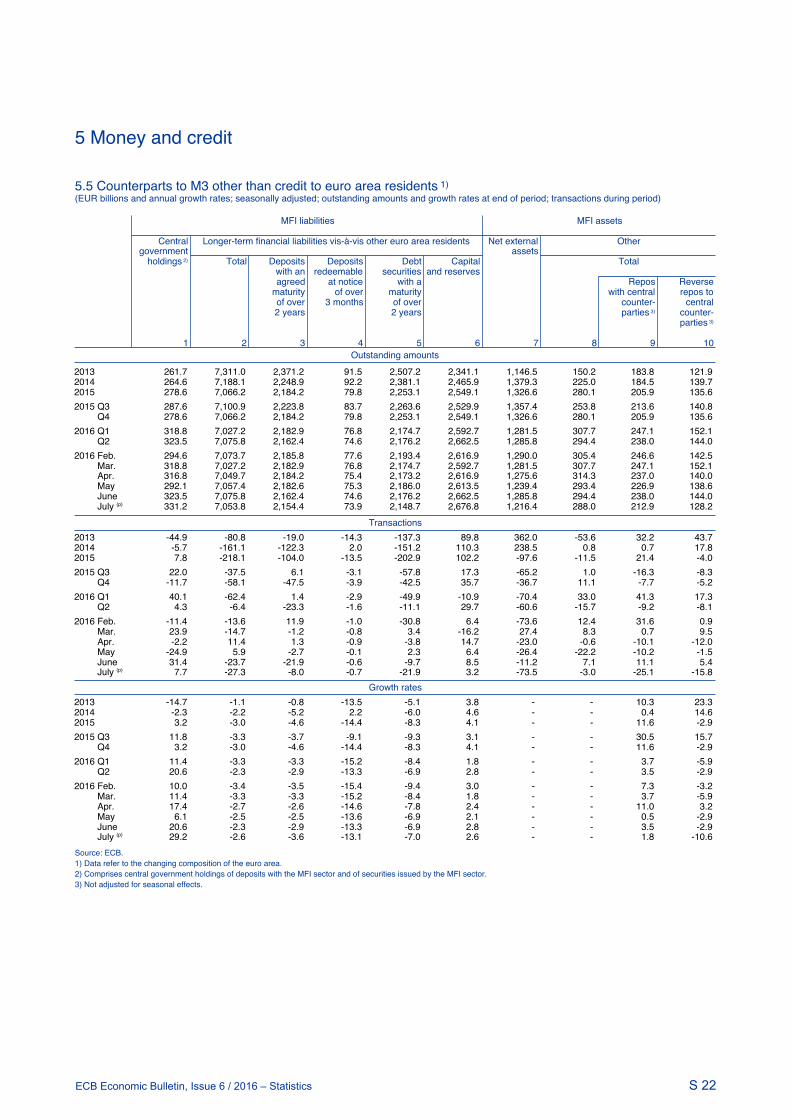
S 22ECB Economic Bulletin, Issue 6 / 2016 – Statistics
5 Money and credit
S 22ECB Economic Bulletin, Issue 6 / 2016 - Statistics
5.5 Counterparts to M3 other than credit to euro area residents 1)(EUR billions and annual growth rates; seasonally adjusted; outstanding amounts and growth rates at end of period; transactions during period)
Outstanding amounts
MFI liabilities MFI assets
Central Longer-term financial liabilities vis-à-vis other euro area residents Net external Other
government assets holdings 2) Total Deposits Deposits Debt Capital Total
with an redeemable securities and reservesagreed at notice with a Repos Reverse
maturity of over maturity with central repos toof over 3 months of over counter- central2 years 2 years parties 3) counter-
parties 3)
1 2 3 4 5 6 7 8 9 10
2013 261.7 7,311.0 2,371.2 91.5 2,507.2 2,341.1 1,146.5 150.2 183.8 121.92014 264.6 7,188.1 2,248.9 92.2 2,381.1 2,465.9 1,379.3 225.0 184.5 139.72015 278.6 7,066.2 2,184.2 79.8 2,253.1 2,549.1 1,326.6 280.1 205.9 135.62015 Q3 287.6 7,100.9 2,223.8 83.7 2,263.6 2,529.9 1,357.4 253.8 213.6 140.8 Q4 278.6 7,066.2 2,184.2 79.8 2,253.1 2,549.1 1,326.6 280.1 205.9 135.62016 Q1 318.8 7,027.2 2,182.9 76.8 2,174.7 2,592.7 1,281.5 307.7 247.1 152.1 Q2 323.5 7,075.8 2,162.4 74.6 2,176.2 2,662.5 1,285.8 294.4 238.0 144.02016 Feb. 294.6 7,073.7 2,185.8 77.6 2,193.4 2,616.9 1,290.0 305.4 246.6 142.5 Mar. 318.8 7,027.2 2,182.9 76.8 2,174.7 2,592.7 1,281.5 307.7 247.1 152.1 Apr. 316.8 7,049.7 2,184.2 75.4 2,173.2 2,616.9 1,275.6 314.3 237.0 140.0 May 292.1 7,057.4 2,182.6 75.3 2,186.0 2,613.5 1,239.4 293.4 226.9 138.6 June 323.5 7,075.8 2,162.4 74.6 2,176.2 2,662.5 1,285.8 294.4 238.0 144.0 July (p) 331.2 7,053.8 2,154.4 73.9 2,148.7 2,676.8 1,216.4 288.0 212.9 128.2
Transactions2013 -44.9 -80.8 -19.0 -14.3 -137.3 89.8 362.0 -53.6 32.2 43.72014 -5.7 -161.1 -122.3 2.0 -151.2 110.3 238.5 0.8 0.7 17.82015 7.8 -218.1 -104.0 -13.5 -202.9 102.2 -97.6 -11.5 21.4 -4.02015 Q3 22.0 -37.5 6.1 -3.1 -57.8 17.3 -65.2 1.0 -16.3 -8.3 Q4 -11.7 -58.1 -47.5 -3.9 -42.5 35.7 -36.7 11.1 -7.7 -5.22016 Q1 40.1 -62.4 1.4 -2.9 -49.9 -10.9 -70.4 33.0 41.3 17.3 Q2 4.3 -6.4 -23.3 -1.6 -11.1 29.7 -60.6 -15.7 -9.2 -8.12016 Feb. -11.4 -13.6 11.9 -1.0 -30.8 6.4 -73.6 12.4 31.6 0.9 Mar. 23.9 -14.7 -1.2 -0.8 3.4 -16.2 27.4 8.3 0.7 9.5 Apr. -2.2 11.4 1.3 -0.9 -3.8 14.7 -23.0 -0.6 -10.1 -12.0 May -24.9 5.9 -2.7 -0.1 2.3 6.4 -26.4 -22.2 -10.2 -1.5 June 31.4 -23.7 -21.9 -0.6 -9.7 8.5 -11.2 7.1 11.1 5.4 July (p) 7.7 -27.3 -8.0 -0.7 -21.9 3.2 -73.5 -3.0 -25.1 -15.8
Growth rates2013 -14.7 -1.1 -0.8 -13.5 -5.1 3.8 - - 10.3 23.32014 -2.3 -2.2 -5.2 2.2 -6.0 4.6 - - 0.4 14.62015 3.2 -3.0 -4.6 -14.4 -8.3 4.1 - - 11.6 -2.92015 Q3 11.8 -3.3 -3.7 -9.1 -9.3 3.1 - - 30.5 15.7 Q4 3.2 -3.0 -4.6 -14.4 -8.3 4.1 - - 11.6 -2.92016 Q1 11.4 -3.3 -3.3 -15.2 -8.4 1.8 - - 3.7 -5.9 Q2 20.6 -2.3 -2.9 -13.3 -6.9 2.8 - - 3.5 -2.92016 Feb. 10.0 -3.4 -3.5 -15.4 -9.4 3.0 - - 7.3 -3.2 Mar. 11.4 -3.3 -3.3 -15.2 -8.4 1.8 - - 3.7 -5.9 Apr. 17.4 -2.7 -2.6 -14.6 -7.8 2.4 - - 11.0 3.2 May 6.1 -2.5 -2.5 -13.6 -6.9 2.1 - - 0.5 -2.9 June 20.6 -2.3 -2.9 -13.3 -6.9 2.8 - - 3.5 -2.9 July (p) 29.2 -2.6 -3.6 -13.1 -7.0 2.6 - - 1.8 -10.6Source: ECB.1) Data refer to the changing composition of the euro area.2) Comprises central government holdings of deposits with the MFI sector and of securities issued by the MFI sector.3) Not adjusted for seasonal effects.
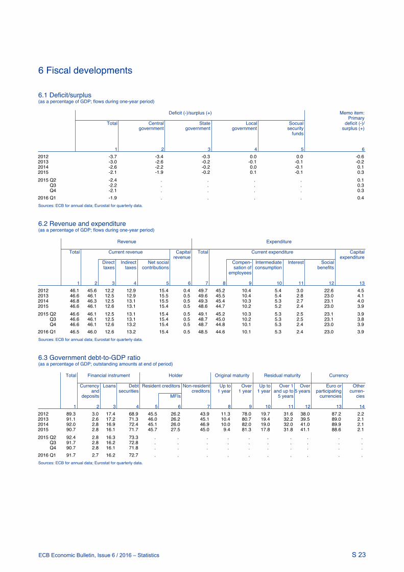
S 23ECB Economic Bulletin, Issue 6 / 2016 – Statistics
6 Fiscal developments
S 23ECB Economic Bulletin, Issue 6 / 2016 - Statistics
6.1 Deficit/surplus(as a percentage of GDP; flows during one-year period)
Deficit (-)/surplus (+) Memo item:Primary
Total Central State Local Socual deficit (-)/government government government security surplus (+)
funds
1 2 3 4 5 62012 -3.7 -3.4 -0.3 0.0 0.0 -0.62013 -3.0 -2.6 -0.2 -0.1 -0.1 -0.22014 -2.6 -2.2 -0.2 0.0 -0.1 0.12015 -2.1 -1.9 -0.2 0.1 -0.1 0.32015 Q2 -2.4 . . . . 0.1 Q3 -2.2 . . . . 0.3 Q4 -2.1 . . . . 0.32016 Q1 -1.9 . . . . 0.4Sources: ECB for annual data; Eurostat for quarterly data.
6.2 Revenue and expenditure(as a percentage of GDP; flows during one-year period)
Revenue Expenditure
Total Current revenue Capital Total Current expenditure Capital
revenue expenditureDirect Indirect Net social Compen- Intermediate Interest Socialtaxes taxes contributions sation of consumption benefits
employees
1 2 3 4 5 6 7 8 9 10 11 12 132012 46.1 45.6 12.2 12.9 15.4 0.4 49.7 45.2 10.4 5.4 3.0 22.6 4.52013 46.6 46.1 12.5 12.9 15.5 0.5 49.6 45.5 10.4 5.4 2.8 23.0 4.12014 46.8 46.3 12.5 13.1 15.5 0.5 49.3 45.4 10.3 5.3 2.7 23.1 4.02015 46.6 46.1 12.6 13.1 15.4 0.5 48.6 44.7 10.2 5.2 2.4 23.0 3.92015 Q2 46.6 46.1 12.5 13.1 15.4 0.5 49.1 45.2 10.3 5.3 2.5 23.1 3.9 Q3 46.6 46.1 12.5 13.1 15.4 0.5 48.7 45.0 10.2 5.3 2.5 23.1 3.8 Q4 46.6 46.1 12.6 13.2 15.4 0.5 48.7 44.8 10.1 5.3 2.4 23.0 3.92016 Q1 46.5 46.0 12.6 13.2 15.4 0.5 48.5 44.6 10.1 5.3 2.4 23.0 3.9Sources: ECB for annual data; Eurostat for quarterly data.
6.3 Government debt-to-GDP ratio(as a percentage of GDP; outstanding amounts at end of period)
Total Financial instrument Holder Original maturity Residual maturity Currency
Currency Loans Debt Resident creditors Non-resident Up to Over Up to Over 1 Over Euro or Otherand securities creditors 1 year 1 year 1 year and up to 5 years participating curren-
deposits MFIs 5 years currencies cies
1 2 3 4 5 6 7 8 9 10 11 12 13 142012 89.3 3.0 17.4 68.9 45.5 26.2 43.9 11.3 78.0 19.7 31.6 38.0 87.2 2.22013 91.1 2.6 17.2 71.3 46.0 26.2 45.1 10.4 80.7 19.4 32.2 39.5 89.0 2.12014 92.0 2.8 16.9 72.4 45.1 26.0 46.9 10.0 82.0 19.0 32.0 41.0 89.9 2.12015 90.7 2.8 16.1 71.7 45.7 27.5 45.0 9.4 81.3 17.8 31.8 41.1 88.6 2.12015 Q2 92.4 2.8 16.3 73.3 . . . . . . . . . . Q3 91.7 2.8 16.2 72.8 . . . . . . . . . . Q4 90.7 2.8 16.1 71.8 . . . . . . . . . . 2016 Q1 91.7 2.7 16.2 72.7 . . . . . . . . . . Sources: ECB for annual data; Eurostat for quarterly data.
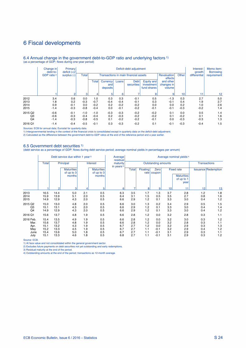
S 24ECB Economic Bulletin, Issue 6 / 2016 – Statistics
6 Fiscal developments
S 24ECB Economic Bulletin, Issue 6 / 2016 - Statistics
6.4 Annual change in the government debt-to-GDP ratio and underlying factors 1)(as a percentage of GDP; flows during one-year period)
Change in Primary Deficit-debt adjustment Interest- Memo item:debt-to- deficit (+)/ growth Borrowing
GDP ratio 2) surplus (-) Total Transactions in main financial assets Revaluation Other differential requirementeffects
Total Currency Loans Debt Equity and and otherand securities investment changes in
deposits fund shares volume
1 2 3 4 5 6 7 8 9 10 11 122012 3.4 0.6 0.0 1.0 0.3 0.3 -0.1 0.5 -1.3 0.3 2.7 5.02013 1.8 0.2 -0.3 -0.7 -0.4 -0.4 -0.1 0.3 -0.1 0.4 1.9 2.72014 0.9 -0.1 0.0 -0.2 0.2 -0.2 -0.2 0.0 0.0 0.2 1.0 2.62015 -1.4 -0.3 -0.8 -0.4 0.0 -0.1 -0.2 -0.1 -0.1 -0.3 -0.2 1.42015 Q2 -0.6 -0.1 -1.0 -1.0 -0.3 -0.3 -0.2 -0.2 0.1 0.0 0.5 1.4 Q3 -0.6 -0.3 -0.4 -0.4 0.2 -0.3 -0.2 -0.2 0.1 -0.2 0.1 1.6 Q4 -1.4 -0.3 -0.8 -0.5 0.1 -0.2 -0.2 -0.1 0.0 -0.3 -0.3 1.32016 Q1 -1.4 -0.4 -0.5 -0.1 0.3 -0.3 -0.2 0.1 -0.1 -0.3 -0.4 1.5Sources: ECB for annual data; Eurostat for quarterly data.1) Intergovernmental lending in the context of the financial crisis is consolidated except in quarterly data on the deficit-debt adjustment.2) Calculated as the difference between the government debt-to-GDP ratios at the end of the reference period and a year earlier.
6.5 Government debt securities 1)(debt service as a percentage of GDP; flows during debt service period; average nominal yields in percentages per annum)
Debt service due within 1 year 2) Average Average nominal yields 4)
residual Total Principal Interest maturity Outstanding amounts Transactions
in years 3)
Maturities Maturities Total Floating Zero Fixed rate Issuance Redemptionof up to 3 of up to 3 rate coupon
months months Maturitiesof up to 1
year
1 2 3 4 5 6 7 8 9 10 11 12 132013 16.5 14.4 5.0 2.1 0.5 6.3 3.5 1.7 1.3 3.7 2.8 1.2 1.82014 15.9 13.9 5.1 2.0 0.5 6.4 3.1 1.5 0.5 3.5 2.7 0.8 1.62015 14.9 12.9 4.3 2.0 0.5 6.6 2.9 1.2 0.1 3.3 3.0 0.4 1.22015 Q2 15.0 13.0 4.8 2.0 0.5 6.6 3.0 1.3 0.2 3.4 2.9 0.5 1.5 Q3 15.1 13.1 4.3 2.0 0.5 6.6 2.9 1.2 0.1 3.3 3.0 0.4 1.4 Q4 14.9 12.9 4.3 2.0 0.5 6.6 2.9 1.2 0.1 3.3 3.0 0.4 1.22016 Q1 15.6 13.7 4.8 1.9 0.5 6.6 2.8 1.2 0.0 3.2 2.8 0.3 1.12016 Feb. 15.4 13.5 4.9 1.9 0.5 6.6 2.8 1.2 0.0 3.2 3.0 0.3 1.2 Mar. 15.6 13.7 4.8 1.9 0.5 6.6 2.8 1.2 0.0 3.2 2.8 0.3 1.1 Apr. 15.1 13.2 4.3 1.9 0.5 6.7 2.7 1.2 0.0 3.2 2.9 0.3 1.3 May 15.2 13.3 4.5 1.9 0.5 6.7 2.7 1.1 -0.1 3.2 2.9 0.4 1.2 June 15.4 13.6 5.0 1.8 0.5 6.7 2.7 1.1 -0.1 3.1 2.9 0.3 1.1 July 15.1 13.3 4.6 1.8 0.5 6.8 2.7 1.1 -0.1 3.1 2.9 0.3 1.2Source: ECB.1) At face value and not consolidated within the general government sector.2) Excludes future payments on debt securities not yet outstanding and early redemptions.3) Residual maturity at the end of the period.4) Outstanding amounts at the end of the period; transactions as 12-month average.

S 25ECB Economic Bulletin, Issue 6 / 2016 – Statistics
6 Fiscal developments
S 25ECB Economic Bulletin, Issue 6 / 2016 - Statistics
6.6 Fiscal developments in euro area countries(as a percentage of GDP; flows during one-year period and outstanding amounts at end of period)
Government deficit (-)/surplus (+)
Belgium Germany Estonia Ireland 1) Greece Spain France Italy Cyprus
1 2 3 4 5 6 7 8 9
2012 -4.2 -0.1 -0.3 -8.0 -8.8 -10.4 -4.8 -2.9 -5.82013 -3.0 -0.1 -0.2 -5.7 -13.0 -6.9 -4.0 -2.9 -4.92014 -3.1 0.3 0.8 -3.8 -3.6 -5.9 -4.0 -3.0 -8.92015 -2.6 0.7 0.4 -2.3 -7.2 -5.1 -3.5 -2.6 -1.02015 Q2 -3.1 0.4 0.6 -2.3 -4.7 -5.4 -4.1 -2.9 -0.4 Q3 -2.9 0.8 0.7 -1.6 -4.4 -5.3 -3.9 -2.7 -0.9 Q4 -2.6 0.6 0.4 -1.8 -7.2 -5.1 -3.6 -2.6 -1.02016 Q1 -2.7 0.7 1.0 -1.5 -5.7 -5.1 -3.3 -2.5 -0.1
Government debt2012 104.1 79.6 9.5 120.1 159.6 85.4 89.6 123.3 79.32013 105.2 77.2 9.9 120.0 177.7 93.7 92.4 129.0 102.52014 106.5 74.7 10.4 107.5 180.1 99.3 95.4 132.5 108.22015 106.0 71.2 9.7 93.8 176.9 99.2 95.8 132.7 108.92015 Q2 109.5 72.6 9.9 91.1 169.4 99.8 97.7 136.0 110.7 Q3 109.1 72.0 9.8 85.9 171.8 99.7 97.1 134.6 110.2 Q4 106.1 71.2 9.7 78.7 176.9 99.2 96.2 132.7 108.92016 Q1 109.2 71.1 9.6 80.4 176.3 100.5 97.5 135.4 109.3
Government deficit (-)/surplus (+)
Latvia Lithuania Luxembourg Malta Netherlands Austria Portugal Slovenia Slovakia Finland
10 11 12 13 14 15 16 17 18 19
2012 -0.8 -3.1 0.3 -3.5 -3.9 -2.2 -5.7 -4.1 -4.3 -2.22013 -0.9 -2.6 0.8 -2.6 -2.4 -1.3 -4.8 -15.0 -2.7 -2.62014 -1.6 -0.7 1.7 -2.0 -2.4 -2.7 -7.2 -5.0 -2.7 -3.22015 -1.3 -0.2 1.2 -1.5 -1.8 -1.2 -4.4 -2.9 -3.0 -2.72015 Q2 -2.1 0.4 1.3 -2.0 -2.1 -2.2 -6.4 -4.5 -2.9 -3.1 Q3 -2.1 0.1 1.2 -1.7 -2.1 -2.5 -3.1 -4.1 -2.6 -2.9 Q4 -1.3 -0.2 1.2 -1.5 -1.9 -1.2 -4.4 -2.9 -3.0 -2.72016 Q1 -0.8 -0.1 1.0 -0.1 -1.6 -1.2 -3.8 -2.8 -2.8 -2.3
Government debt2012 41.4 39.8 22.0 67.5 66.4 81.6 126.2 53.9 52.4 52.92013 39.1 38.8 23.3 68.6 67.9 80.8 129.0 71.0 55.0 55.52014 40.8 40.7 22.9 67.1 68.2 84.3 130.2 81.0 53.9 59.32015 36.4 42.7 21.4 63.9 65.1 86.2 129.0 83.2 52.9 63.12015 Q2 35.3 37.6 21.8 67.2 67.0 86.3 128.4 81.0 54.7 62.0 Q3 36.4 38.2 21.5 66.0 66.2 86.3 130.2 84.4 53.9 60.6 Q4 36.4 42.8 21.5 63.8 65.1 86.2 129.0 83.2 52.9 62.62016 Q1 38.5 40.1 21.8 65.3 64.8 86.9 128.9 83.6 52.2 63.6Source: Eurostat.1) Differences may occur between quarterly and annual ratios owing to data vintages.
For more information see Eurostatʼs explanatory note (http://ec.europa.eu/eurostat/documents/24987/6390465/Irish_GDP_communication.pdf).

© European Central Bank, 2016
Postal address 60640 Frankfurt am Main, Germany Telephone +49 69 1344 0 Website www.ecb.europa.eu
All rights reserved. Reproduction for educational and non-commercial purposes is permitted provided that the source is acknowledged.
This Bulletin was produced under the responsibility of the Executive Board of the ECB. Translations are prepared and published by the national central banks.
The cut-off date for the statistics included in this issue was 7 September 2016.
ISSN 2363-3417 (epub) ISSN 2363-3417 (html) ISSN 2363-3417 (pdf) EU catalogue No QB-BP-16-006-EN-E (epub) EU catalogue No QB-BP-16-006-EN-Q (html) EU catalogue No QB-BP-16-006-EN-N (pdf)