ec 6511 digital signal processing lab...
TRANSCRIPT

EC 6511 DIGITAL SIGNAL PROCESSING LAB MANUAL
www.studentsfocus.com
EC 6511 DIGITAL SIGNAL PROCESSING LAB MANUAL
S.SUMATHI , AP/ECE Page 2
INTRODUCTION
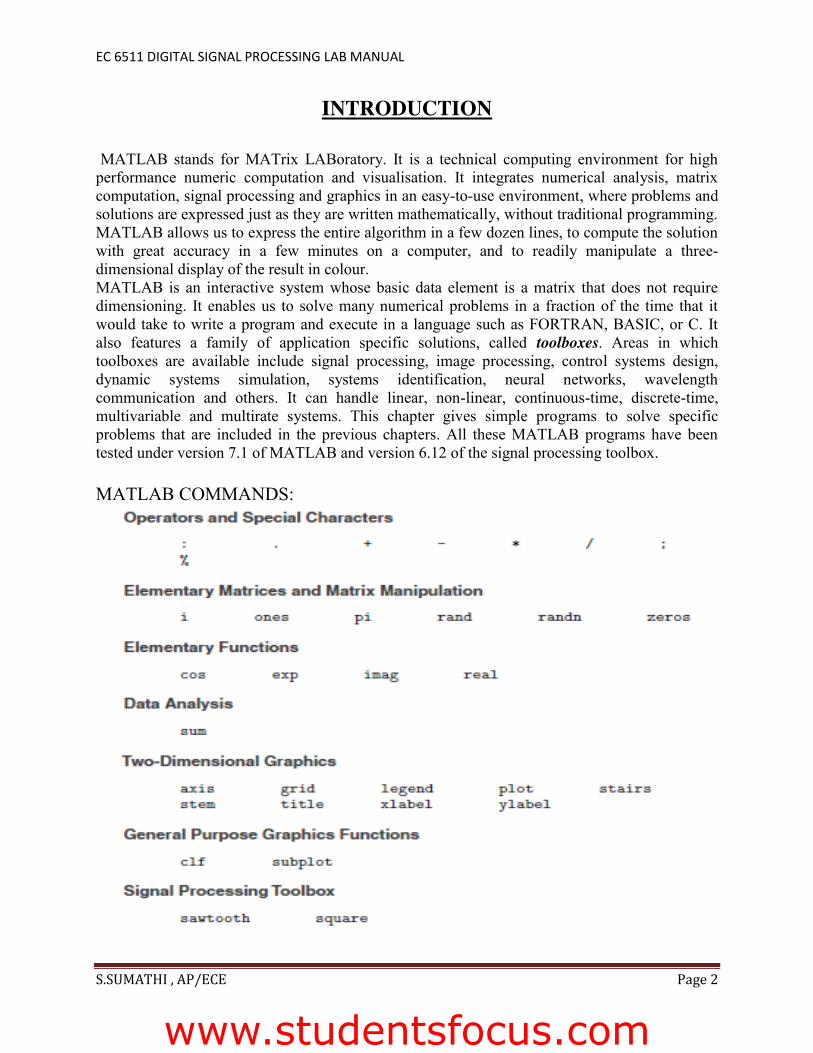
MATLAB stands for MATrix LABoratory. It is a technical computing environment for high performance numeric computation and visualisation. It integrates numerical analysis, matrix computation, signal processing and graphics in an easy-to-use environment, where problems and solutions are expressed just as they are written mathematically, without traditional programming. MATLAB allows us to express the entire algorithm in a few dozen lines, to compute the solution with great accuracy in a few minutes on a computer, and to readily manipulate a three-dimensional display of the result in colour. MATLAB is an interactive system whose basic data element is a matrix that does not require dimensioning. It enables us to solve many numerical problems in a fraction of the time that it would take to write a program and execute in a language such as FORTRAN, BASIC, or C. It also features a family of application specific solutions, called toolboxes. Areas in which toolboxes are available include signal processing, image processing, control systems design, dynamic systems simulation, systems identification, neural networks, wavelength communication and others. It can handle linear, non-linear, continuous-time, discrete-time, multivariable and multirate systems. This chapter gives simple programs to solve specific problems that are included in the previous chapters. All these MATLAB programs have been tested under version 7.1 of MATLAB and version 6.12 of the signal processing toolbox. MATLAB COMMANDS:
www.studentsfocus.com

EC 6511 DIGITAL SIGNAL PROCESSING LAB MANUAL
S.SUMATHI , AP/ECE Page 3
GENERATION OF SIGNALS 1.A. CONTINUOUS TIME SIGNAL
Aim To Generate a continuous sinusoidal time signals Using MATLAB. Requirements Matlab 2007 SOFTWARE Procedure
1. OPEN MATLAB
2. File New Script.
a. Type the program in untitled window
3. File Save type filename.m in matlab workspace path
4. Debug Run. Wave will displayed at Figure dialog box.
Theory Common Periodic Waveforms The toolbox provides functions for generating widely used periodic waveforms:sawtooth generates a sawtooth wave with peaks at ±1 and a period of 2π. An optional width parameter specifies a fractional multiple of 2π at which the signal's maximum occurs. square generates a square wave with a period of 2π. An optional parameter specifies duty cycle, the percent of the period for which the signal is positive.
Common Aperiodic Waveforms The toolbox also provides functions for generating several widely used aperiodic waveforms: gauspuls generates a Gaussian-modulated sinusoidal pulse with a specified time, center frequency, and fractional bandwidth. Optional parameters return in-phase and Quadrature pulses, the RF signal envelope, and the cutoff time for the trailing pulse envelope. chirp generates a linear, log, or quadratic swept-frequency cosine signal. An optional parameter specifies alternative sweep methods. An optional parameter phi allows initial phase to be specified in degrees. Program %
www.studentsfocus.com

EC 6511 DIGITAL SIGNAL PROCESSING LAB MANUAL
S.SUMATHI , AP/ECE Page 4
% Assuming The Sampling frequency is 5 Mhz
clc;
clear all; t = 0:0.0005:1;
a = 10
f = 13;
xa = a*sin(2*pi*f*t);
subplot(2,1,1)
plot(t,xa);grid
xlabel('Time, msec');
ylabel('Amplitude');
title('Continuous-time signal x_{a}(t)');
axis([0 1 -10.2 10.2])
clear all;
Finput = 1000;
Fsampling = 5000000;
Tsampling = 1 / Fsampling;
Nsample = Fsampling/ Finput;
N = 0:5*Nsample-1;
x=sin(2 * pi * Finput * Tsampling * N);
plot(x); title('Sine Wave Generation');
xlabel('Time -- >');
ylabel('Amplitude-- >');
grid on;
Result
Thus the Continuous Time Signal was generated using MATLAB.
www.studentsfocus.com

EC 6511 DIGITAL SIGNAL PROCESSING LAB MANUAL
S.SUMATHI , AP/ECE Page 5
1.B. DISCRETE TIME SIGNAL Aim To Generate a Discrete time Exponential signals Using MATLAB. Requirements Matlab 2007 Personal computer Procedure
1. OPEN MATLAB
2. File New Script. a. Type the program in untitled window 3. File Save type filename.m in matlab workspace path
4. Debug Run. Wave will displayed at Figure dialog box. Theory: Program clear all;
a = 10; f = 13; T = 0.01; n = 0:T:1; xs = a*sin(2*pi*f*n); k = 0:length(n)-1; stem(k,xs); grid xlabel('Time index n'); ylabel('Amplitude'); title('Discrete-time signal x[n]'); axis([0 (length(n)-1) -10.2 10.2])
www.studentsfocus.com

EC 6511 DIGITAL SIGNAL PROCESSING LAB MANUAL
S.SUMATHI , AP/ECE Page 6
Expected Graph:
Result
Thus the Discrete Time Signal was generated using MATLAB.
www.vidyarthiplus.com
www.vidyarthiplus.com
www.studentsfocus.com

EC 6511 DIGITAL SIGNAL PROCESSING LAB MANUAL
S.SUMATHI , AP/ECE Page 7
GENERATIONS OF ELEMENTRY SEQUENCES
Aim : To develop elementary signal function modules (m-files) for unit sample, unit step, exponential and unit ramp sequences.
Apparatus :
PC having MATLAB software.
Program :
% program for generation of unit sample
clc;clear all;close all;
t = -3:1:3;
y = [zeros(1,3),ones(1,1),zeros(1,3)];
subplot(2,2,1);stem(t,y);
ylabel('Amplitude------>');
xlabel('(a)n ------>');
title('Unit Impulse Signal');
% program for genration of unit step of sequence [u(n)- u(n)-N]
t = -4:1:4;
y1 = ones(1,9);
subplot(2,2,2);stem(t,y1);
ylabel('Amplitude------>');
xlabel('(b)n ------>');
title('Unit step');
% program for generation of ramp signal
n1 = input('Enter the value for end of the seqeuence '); %n1 = <any value>7 %
x = 0:n1;
subplot(2,2,3);stem(x,x);
ylabel('Amplitude------>');
www.vidyarthiplus.com
www.vidyarthiplus.com
www.studentsfocus.com

EC 6511 DIGITAL SIGNAL PROCESSING LAB MANUAL
S.SUMATHI , AP/ECE Page 8
xlabel('(c)n ------>');
title('Ramp sequence');
% program for generation of exponential signal
n2 = input('Enter the length of exponential seqeuence '); %n2 = <any value>7 %
t = 0:n2;
a = input('Enter the Amplitude'); %a=1%
y2 = exp(a*t);
subplot(2,2,4);stem(t,y2);
ylabel('Amplitude------>');
xlabel('(d)n ------>');
title('Exponential sequence');
disp('Unit impulse signal');y
disp('Unit step signal');y1
disp('Unit Ramp signal');x
disp('Exponential signal');x
Output :
Enter the value for end of the seqeuence 6
Enter the length of exponential seqeuence 4
Enter the Amplitude1
Unit impulse signal y = 0 0 0 1 0 0 0
Unit step signal y1 = 1 1 1 1 1 1 1 1 1
Unit Ramp signal x = 0 1 2 3 4 5 6
Exponential signal x = 0 1 2 3 4 5 6
www.vidyarthiplus.com
www.vidyarthiplus.com
www.studentsfocus.com

EC 6511 DIGITAL SIGNAL PROCESSING LAB MANUAL
S.SUMATHI , AP/ECE Page 9
Graph:
Result
Thus the different sequences were generated using MATLAB.
-4 -2 0 2 40
0.5
1Am
plitu
de---
--->
(a)n ------>
Unit Impulse Signal
-4 -2 0 2 40
0.5
1
Ampl
itude
------
>
(b)n ------>
Unit step
0 2 4 60
2
4
6
Ampl
itude
------
>
(c)n ------>
Ramp sequence
0 1 2 3 40
20
40
60
Ampl
itude
------
>
(d)n ------>
Exponential sequence
www.vidyarthiplus.com
www.vidyarthiplus.com
www.studentsfocus.com

EC 6511 DIGITAL SIGNAL PROCESSING LAB MANUAL
S.SUMATHI , AP/ECE Page 10
BASIC OPERATIONS ON SIGNALS Aim :
To develop program for some basic operations like addition, subtraction, shifting and folding on signal.
Apparatus :
PC having MATLAB software.
Theory:
Basic Operations Signal Adding:
This is a sample-by-sample addition given by and the length of x1(n) and x2(n) must be the same
n)}={x1 n)}
Signal Multiplication: This is a sample-by-sample multiplication (or “dot” multiplication) given by
PROGRAM:
www.vidyarthiplus.com
www.vidyarthiplus.com
www.studentsfocus.com

EC 6511 DIGITAL SIGNAL PROCESSING LAB MANUAL
S.SUMATHI , AP/ECE Page 11
ADDITION:
x=input(„ENTER THE FIRST SEQUENCE:‟); subplot(3,1,1); stem(x); title('X'); y=input(„ENTER THE SECOND SEQUENCE:‟); subplot(3,1,2); stem(y); title('Y'); z=x+y; disp(z) subplot(3,1,3); stem(z); title('Z=X+Y'); OUTPUT: ENTER THE FIRST SEQUENCE:[2 3 1 4 5] ENTER THE SECOND SEQUENCE:[1 -1 0 1 -1] 3 2 1 5 4 EXPECTED GRAPH:
www.vidyarthiplus.com
www.vidyarthiplus.com
www.studentsfocus.com

EC 6511 DIGITAL SIGNAL PROCESSING LAB MANUAL
S.SUMATHI , AP/ECE Page 12
SUBTRACTION clc; clear all; close all; n1=-2:1; x=input('ENTER THE FIRST SEQUENCE:'); n2=0:3; y=input('ENTER THE SECOND SEQUENCE:'); subplot(3,1,1); stem(n1,x); xlabel ('time') ylabel ('amplitude') title('FIRST SEQUENCE') ; axis([-4 4 -5 5]); subplot(3,1,2); stem(n2,y); xlabel ('time') ylabel ('amplitude') title('SECOND SEQUENCE'); axis([-4 4 -5 5]); n3 =min (min(n1) ,min( n2 ) ) : max ( max ( n1 ) , max ( n2 ) ); % finding the duration of output signal s1 =zeros(1,length (n3) ); s2 =s1; s1 (find ( ( n3>=min( n1 ) ) & ( n3 <=max ( n1 ) )==1 ) )=x; % signal x with the duration of output signal 'sub' s2 (find ( ( n3>=min ( n2 ) ) & ( n3 <=max ( n2 ))==1) )=y; % signal y with the duration of output signal 'sub' sub=s1 - s2; % subtraction disp('subtracted sequence') disp(sub) subplot(3,1,3) stem(n3,sub) xlabel ('time') ylabel ('amplitude') OUTPUT: ENTER THE FIRST SEQUENCE:[2 4 6 8] ENTER THE SECOND SEQUENCE:[1 3 5 7] subtracted sequence 2 4 5 5 -5 -7
www.vidyarthiplus.com
www.vidyarthiplus.com
www.studentsfocus.com

EC 6511 DIGITAL SIGNAL PROCESSING LAB MANUAL
S.SUMATHI , AP/ECE Page 13
EXPECTED GRAPH:
MULTIPLICATION PROGRAM: clc; clear all; close all; n1=-2:1; x=input('ENTER THE FIRST SEQUENCE:'); n2=0:3; y=input('ENTER THE SECOND SEQUENCE:'); subplot(3,1,1); stem(n1,x); xlabel ('time') ylabel ('amplitude') title('FIRST SEQUENCE') ; axis([-4 4 -5 5]); subplot(3,1,2); stem(n2,y); xlabel ('time') ylabel ('amplitude') title('SECOND SEQUENCE'); axis([-4 4 -5 5]); n3 =min (min(n1) ,min( n2 ) ) : max ( max ( n1 ) , max ( n2 ) ); % finding the duration of output signal (out)
www.vidyarthiplus.com
www.vidyarthiplus.com
www.studentsfocus.com

EC 6511 DIGITAL SIGNAL PROCESSING LAB MANUAL
S.SUMATHI , AP/ECE Page 14
s1 =zeros(1,length (n3) ); s2 =s1; s1 (find ( ( n3>=min( n1 ) ) & ( n3 <=max ( n1 ) )==1 ) )=x; % signal x with the duration of output signal 'mul' s2 (find ( ( n3>=min ( n2 ) ) & ( n3 <=max ( n2 ))==1) )=y; % signal y with the duration of output signal 'mul' mul=s1 .* s2; % multiplication disp('MULTIPLIED SEQUENCE') disp(mul) subplot(3,1,3) stem(n3,mul) xlabel ('time') ylabel ('amplitude') OUTPUT: ENTER THE FIRST SEQUENCE:[2 4 6 8] ENTER THE SECOND SEQUENCE:[2 3 4 5] MULTIPLIED SEQUENCE 0 0 12 24 0 0 EXPECTED GRAPH:
www.vidyarthiplus.com
www.vidyarthiplus.com
www.studentsfocus.com

EC 6511 DIGITAL SIGNAL PROCESSING LAB MANUAL
S.SUMATHI , AP/ECE Page 15
SHIFTING PROGRAM: clc; clear all; close all; n1=input('Enter the amount to be delayed'); n2=input('Enter the amount to be advanced'); n=-2:2; x=input('ENTER THE SEQUENCE'); subplot(3,1,1); stem(n,x); title('Signal x(n)'); m=n+n1; y=x; subplot(3,1,2); stem(m,y); title('Delayed signal x(n-n1)'); t=n-n2; z=x; subplot(3,1,3); stem(t,z); title('Advanced signal x(n+n2)'); OUTPUT: Enter the amount to be delayed 3 Enter the amount to be advanced4 ENTER THE SEQUENCE[1 2 3 4 5] EXPECTED GRAPH:
www.vidyarthiplus.com
www.vidyarthiplus.com
www.studentsfocus.com

EC 6511 DIGITAL SIGNAL PROCESSING LAB MANUAL
S.SUMATHI , AP/ECE Page 16
FOLDING or REVERSING: PROGRAM: clc; clear all; close all; n=-1:2; x=input('ENTER THE SEQUENCE'); subplot(2,1,1) stem(n,x); axis([-3 3 -5 5]); title('Signal x(n)'); c=fliplr(x); y=fliplr(-n); disp('FOLDED SEQUENCE') disp(c) subplot(2,1,2); stem(y,c); axis([-3 3 -5 5]); title('Reversed Signal x(-n)') ; OUTPUT: ENTER THE SEQUENCE[1 -1 2 -3] FOLDED SEQUENCE -3 2 -1 1
www.vidyarthiplus.com
www.vidyarthiplus.com
www.studentsfocus.com

EC 6511 DIGITAL SIGNAL PROCESSING LAB MANUAL
S.SUMATHI , AP/ECE Page 17
EXPECTED GRAPH
Result
Thus the different operations on sequences were verified using MATLAB.
www.vidyarthiplus.com
www.vidyarthiplus.com
www.studentsfocus.com

EC 6511 DIGITAL SIGNAL PROCESSING LAB MANUAL
S.SUMATHI , AP/ECE Page 18
CORRELATION Aim :
To develop program for correlation.
Apparatus :
PC having MATLAB software.
Program :
CROSS CORRELATION % Program for computing cross-correlation of the sequences x5[1, 2, 3, 4] and h5[4, 3, 2, 1]
clc; clear all; close all; x=input(„enter the 1st sequence‟); h=input(„enter the 2nd sequence‟); y=crosscorr(x,h); figure; subplot(3,1,1); stem(x); ylabel(„Amplitude --.‟); xlabel(„(a) n --.‟); title(„input sequence‟); subplot(3,1,2); stem(h); ylabel(„Amplitude --.‟); xlabel(„(b) n --.‟); title(„impulse sequence‟); subplot(3,1,3); stem(fliplr(y));
ylabel(„Amplitude --.‟);
xlabel(„(c) n --.‟); title(„Cross correlated sequence‟); disp(„The resultant signal is‟);
fliplr(y)
OUTPUT: enter the 1st sequence [1 2 3 4] enter the 2nd sequence [4 3 2 1] The resultant signal is Y=1.0000 4.0000 10.0000 20.↑0000 25.0000 24.0000 16.0000
www.vidyarthiplus.com
www.vidyarthiplus.com
www.studentsfocus.com

EC 6511 DIGITAL SIGNAL PROCESSING LAB MANUAL
S.SUMATHI , AP/ECE Page 19
EXPECTED GRAPH:
AUTO CORRELATION
% Program for computing autocorrelation function
x=input(„enter the sequence‟); y=crosscorr(x,x); figure;subplot(2,1,1); stem(x);ylabel(„Amplitude --.‟); xlabel(„(a) n --.‟); title(„original signal‟); subplot(2,1,2); stem(fliplr(y));ylabel(„Amplitude --.‟); xlabel(„(a) n --.‟); title („Auto correlated sequence‟);
disp(„The resultant signal is‟);
fliplr(y)
www.vidyarthiplus.com
www.vidyarthiplus.com
www.studentsfocus.com

EC 6511 DIGITAL SIGNAL PROCESSING LAB MANUAL
S.SUMATHI , AP/ECE Page 20
OUTPUT: enter the sequence [1 2 3 4] The resultant signal is Y=4 11 20 ↑30 20 11 4
EXPECTED GRAPH:
RESULT:
Thus correlation of two signals ACHIEVED using MATLAB.
www.vidyarthiplus.com
www.vidyarthiplus.com
www.studentsfocus.com

EC 6511 DIGITAL SIGNAL PROCESSING LAB MANUAL
S.SUMATHI , AP/ECE Page 21
LINEAR CONVOLUTION
Aim To perform a Linear Convolution Using MATLAB. Requirements Matlab 2007 later Procedure 1. OPEN MATLAB
2. File New Script.
a. Type the program in untitled window 3. File Save type filename.m in matlab workspace path
4. Debug Run. Wave will displayed at Figure dialog box.
Program % Program for linear convolution of the sequence x5[1, 2] and h5[1, 2, 4]
clc; clear all; close all; x=input('enter the 1st sequence'); h=input('enter the 2nd sequence'); y=conv(x,h); figure; subplot(3,1,1); stem(x); ylabel('Amplitude --.'); xlabel('(a) n --.'); title('first sequence'); subplot(3,1,2); stem(h);ylabel('Amplitude --.'); xlabel('(b) n --.'); title('Second sequence'); subplot(3,1,3); stem(y); ylabel('Amplitude --.'); xlabel('(c) n --.'); title('Convoluted sequence');
www.vidyarthiplus.com
www.vidyarthiplus.com
www.studentsfocus.com

EC 6511 DIGITAL SIGNAL PROCESSING LAB MANUAL
S.SUMATHI , AP/ECE Page 22
disp('The resultant signal is'); Output: enter the 1st sequence [1 2] enter the 2nd sequence [1 2 4] The resultant signal is Y= 1 4 8 8 EXPECTED GRAPHS:
Result Thus the Linear convolution was performed using MATLAB.
www.vidyarthiplus.com
www.vidyarthiplus.com
www.studentsfocus.com

EC 6511 DIGITAL SIGNAL PROCESSING LAB MANUAL
S.SUMATHI , AP/ECE Page 23
CIRCULAR CONVOLUTION Aim To perform a Circular Convolution Using MATLAB. Requirements Matlab 2007 later Procedure 1. OPEN MATLAB
2. File New Script. a. Type the program in untitled window 3. File Save type filename.m in matlab workspace path
4. Debug Run. Wave will displayed at Figure dialog box. Program clc; clear all; a = input(„enter the sequence x(n) = ‟); b = input(„enter the sequence h(n) = ‟); n1=length(a); n2=length(b); N=max(n1,n2); x = [a zeros(1,(N-n1))]; for i = 1:N k = i; for j = 1:n2 H(i,j)=x(k)* b(j); k = k-1; if (k == 0) k = N; end end end y=zeros(1,N); M=H‟; for j = 1:N for i = 1:n2 y(j)=M(i,j)+y(j); end end disp(„The output sequence is y(n)= „); disp(y);
www.vidyarthiplus.com
www.vidyarthiplus.com
www.studentsfocus.com

EC 6511 DIGITAL SIGNAL PROCESSING LAB MANUAL
S.SUMATHI , AP/ECE Page 24
stem(y); title(„Circular Convolution‟); xlabel(„n‟); ylabel(‚y(n)„); OUTPUT: enter the sequence x(n) = [1 2 4] enter the sequence h(n) = [1 2] The output sequence is y(n)= 9 4 8
% Program for Computing Circular Convolution with zero padding
clc; close all; clear all; x=input('enter the first sequence'); h=input('enter the 2nd sequence'); y=x'*h; n1=length(x); n2=length(h); figure subplot(3,1,1) stem(x); title('Input sequence'); xlabel('n1'); ylabel('x(n1)'); subplot(3,1,2) stem(h); title('Impulse sequence'); xlabel('n2'); ylabel('h(n2)'); n=n1+n2-1; c=zeros(n); for i=1:n1 for j=1:n2 c(i+j-1)=c(i+j-1)+y(i,j); end end for i=1:n d(i)=c(i,1); end disp('convoluted sequence'); disp(d); n3=1:n; subplot(3,1,3) stem(n3-1,c); title('Convoluted sequence'); xlabel('time');
www.vidyarthiplus.com
www.vidyarthiplus.com
www.studentsfocus.com

EC 6511 DIGITAL SIGNAL PROCESSING LAB MANUAL
S.SUMATHI , AP/ECE Page 25
ylabel('Amplitude'); OUTPUT: enter the first sequence [1 2 4] enter the 2nd sequence [1 2] The resultant signal is y=1 4 8 8 Result Thus the Circular convolution was performed using MATLAB.
www.vidyarthiplus.com
www.vidyarthiplus.com
www.studentsfocus.com

EC 6511 DIGITAL SIGNAL PROCESSING LAB MANUAL
S.SUMATHI , AP/ECE Page 26
SAMPLING AND EFFECT OF ALIASING
Aim To perform a Sampling and effect of aliasing Using MATLAB. Requirements Matlab 2007 later Procedure 1. OPEN MATLAB
2. File New Script. a. Type the program in untitled window 3. File Save type filename.m in matlab workspace path
4. Debug Run. Wave will displayed at Figure dialog box. Program clc; close all; clear all; f1=1/128; f2=5/128; n=0:255; fc=50/128; x=cos(2*pi*f1*n); x1=cos(2*pi*f2*n); xa=cos(2*pi*fc*n); xamp=x.*xa; subplot(2,2,1);plot(n,x);title('x(n)'); xlabel('n --.');ylabel('amplitude'); subplot(2,2,2);plot(n,xa);title('xa(n)'); xlabel('n --.');ylabel('amplitude'); subplot(2,2,3);plot(n,xamp); xlabel('n --.');ylabel('amplitude');
www.vidyarthiplus.com
www.vidyarthiplus.com
www.studentsfocus.com

EC 6511 DIGITAL SIGNAL PROCESSING LAB MANUAL
S.SUMATHI , AP/ECE Page 27
EXPECTED GRAPH:
Result Thus the Sampling was performed and studied the aliasing effect using MATLAB.
www.vidyarthiplus.com
www.vidyarthiplus.com
www.studentsfocus.com

EC 6511 DIGITAL SIGNAL PROCESSING LAB MANUAL
S.SUMATHI , AP/ECE Page 28
DFT/IDFT of a sequence without using the inbuilt functions AIM: To find the DFT/IDFT of a sequence without using the inbuilt functions EQUIPMENT REQUIRED:
P – IV Computer Windows Xp SP2 MATLAB 7.0
PROGRAM: %program to find the DFT/IDFT of a sequence without using the inbuilt functions clc close all; clear all; xn=input('Enter the sequence x(n)'); %Get the sequence from user ln=length(xn); %find the length of the sequence xk=zeros(1,ln); %initilise an array of same size as that of input sequence ixk=zeros(1,ln); %initilise an array of same size as that of input sequence %code block to find the DFT of the sequence %----------------------------------------------------------- for k=0:ln-1 for n=0:ln-1 xk(k+1)=xk(k+1)+(xn(n+1)*exp((-i)*2*pi*k*n/ln)); end end %------------------------------------------------------------ %code block to plot the input sequence %------------------------------------------------------------ t=0:ln-1; subplot(221); stem(t,xn); grid ylabel ('Amplitude'); xlabel ('Time Index'); title('Input Sequence'); %--------------------------------------------------------------- magnitude=abs(xk); % Find the magnitudes of individual DFT points %code block to plot the magnitude response %------------------------------------------------------------ t=0:ln-1; subplot(222); stem(t,magnitude); grid
www.vidyarthiplus.com
www.vidyarthiplus.com
www.studentsfocus.com

EC 6511 DIGITAL SIGNAL PROCESSING LAB MANUAL
S.SUMATHI , AP/ECE Page 29
ylabel ('Amplitude'); xlabel ('K'); title ('Magnitude Response'); %------------------------------------------------------------ phase=angle(xk); % Find the phases of individual DFT points %code block to plot the magnitude sequence %------------------------------------------------------------ t=0:ln-1; subplot(223); stem(t,phase); grid ylabel ('Phase'); xlabel ('K'); title('Phase Response'); %------------------------------------------------------------ % Code block to find the IDFT of the sequence %------------------------------------------------------------ for n=0:ln-1 for k=0:ln-1 ixk(n+1)=ixk(n+1)+(xk(k+1)*exp(i*2*pi*k*n/ln)); end end ixk=ixk./ln; %------------------------------------------------------------ %code block to plot the input sequence %------------------------------------------------------------ t=0:ln-1; subplot(224); stem(t,xn); grid; ylabel ('Amplitude'); xlabel ('Time Index'); title ('IDFT sequence'); OUTPUT: Enter the sequence x(n) [1 2 3 4]
www.vidyarthiplus.com
www.vidyarthiplus.com
www.studentsfocus.com

EC 6511 DIGITAL SIGNAL PROCESSING LAB MANUAL
S.SUMATHI , AP/ECE Page 30
Expected Output Waveform:
RESULT: Thus the DFT/IDFT of a sequence found without using the inbuilt functions of MATLAB
www.vidyarthiplus.com
www.vidyarthiplus.com
www.studentsfocus.com

EC 6511 DIGITAL SIGNAL PROCESSING LAB MANUAL
S.SUMATHI , AP/ECE Page 31
IMPLEMENTATION OF FFT OF GIVEN SEQUENCE AIM: Implementation of FFT of given sequence and obtain the magnitude and phase response of the same. EQUIPMENT REQUIRED: P – IV Computer Windows Xp SP2 MATLAB 7.0
PROGRAM %To compute the FFT of the impulse sequence and plot magnitude and phase response clc; clear all; close all; %impulse sequence t=-2:1:2; y=[zeros(1,2) 1 zeros(1,2)]; subplot (3,1,1); stem(t,y); title('impulse sequence'); grid; xlabel ('time -->'); ylabel ('--> Amplitude'); xn=y; N=input('enter the length of the FFT sequence: '); xk=fft(xn,N); magxk=abs(xk); angxk=angle(xk); k=0:N-1; subplot(3,1,2); stem(k,magxk); grid; xlabel('k'); ylabel('|x(k)|'); title('magnitude response'); subplot(3,1,3); stem(k,angxk); disp(xk); grid; xlabel('k'); ylabel('arg(x(k))'); title('angle response');
www.vidyarthiplus.com
www.vidyarthiplus.com
www.studentsfocus.com

EC 6511 DIGITAL SIGNAL PROCESSING LAB MANUAL
S.SUMATHI , AP/ECE Page 32
outputs: y= 0 0 1 0 0 enter the length of the FFT sequence: 10 1.0000 0.3090 - 0.9511i -0.8090 - 0.5878i -0.8090 + 0.5878i 0.3090 + 0.9511i 1.0000 0.3090 - 0.9511i -0.8090 - 0.5878i -0.8090 + 0.5878i 0.3090 + 0.9511i
Expected Output:
To compute the FFT of the step sequence and plot magnitude and phase response clc; clear all; close all; %Step Sequence s=input ('enter the length of step sequence'); t=-s:1:s; y=[zeros(1,s) ones(1,1) ones(1,s)]; subplot(3,1,1);
www.vidyarthiplus.com
www.vidyarthiplus.com
www.studentsfocus.com

EC 6511 DIGITAL SIGNAL PROCESSING LAB MANUAL
S.SUMATHI , AP/ECE Page 33
stem(t,y); grid input('y='); disp(y); title ('Step Sequence'); xlabel ('time -->'); ylabel ('--> Amplitude'); xn=y; N=input('enter the length of the FFT sequence: '); xk=fft(xn,N); magxk=abs(xk); angxk=angle(xk); k=0:N-1; subplot(3,1,2); stem(k,magxk); grid xlabel('k'); ylabel('|x(k)|'); subplot(3,1,3); stem(k,angxk); disp(xk); grid xlabel('k'); ylabel('arg(x(k))'); outputs: enter the length of step sequence: 5 y= 0 0 0 0 0 1 1 1 1 1 1 enter the length of the FFT sequence: 10 5.0000 -1.0000 + 3.0777i 0 -1.0000 + 0.7265i 0 -1.0000 0 -1.0000 - 0.7265i 0 -1.0000 - 3.0777i EXPECTED WAVEFORMS
www.vidyarthiplus.com
www.vidyarthiplus.com
www.studentsfocus.com

EC 6511 DIGITAL SIGNAL PROCESSING LAB MANUAL
S.SUMATHI , AP/ECE Page 34
%To compute the FFT of the Exponential sequence and plot magnitude and phase response clc; clear all; close all; %exponential sequence n=input('enter the length of exponential sequence: '); t=0:1:n; a=input('enter "a" value: '); y=exp(a*t); input('y=') disp(y); subplot(3,1,1); stem(t,y); grid; title('exponential response'); xlabel('time'); ylabel('amplitude'); disp(y); xn=y; N=input('enter the length of the FFT sequence: '); xk=fft(xn,N);
www.vidyarthiplus.com
www.vidyarthiplus.com
www.studentsfocus.com

EC 6511 DIGITAL SIGNAL PROCESSING LAB MANUAL
S.SUMATHI , AP/ECE Page 35
magxk=abs(xk); angxk=angle(xk); k=0:N-1; subplot(3,1,2); stem(k,magxk); grid; xlabel('k'); ylabel('|x(k)|'); subplot(3,1,3); stem(k,angxk); grid; disp(xk); xlabel('k'); ylabel('arg(x(k))'); OUTPUTS: enter the length of exponential sequence: 5 enter "a" value: 0.8 y= 1.0000 2.2255 4.9530 11.0232 24.5325 54.5982 enter the length of the FFT sequence: 10 98.3324 -73.5207 -30.9223i 50.9418 +24.7831i -41.7941 -16.0579i 38.8873 + 7.3387i -37.3613 38.8873 - 7.3387i -41.7941 +16.0579i 50.9418 -24.7831i -73.5207 +30.9223i EXPECTED WAVEFORMS
www.vidyarthiplus.com
www.vidyarthiplus.com
www.studentsfocus.com

EC 6511 DIGITAL SIGNAL PROCESSING LAB MANUAL
S.SUMATHI , AP/ECE Page 36
%To compute the FFT for the given sequence and plot magnitude and phase response clc; clear all; close all; %exponential sequence n=input('enter the length of input sequence: '); t=0:1:n; y=input('enter the input sequence'); disp(y); subplot(3,1,1); stem(t,y); grid; title('input sequence'); xlabel('time'); ylabel('amplitude'); disp(y); xn=y; N=input('enter the length of the FFT sequence: '); xk=fft(xn,N); magxk=abs(xk); angxk=angle(xk); k=0:N-1; subplot(3,1,2); stem(k,magxk); grid; xlabel('k');
www.vidyarthiplus.com
www.vidyarthiplus.com
www.studentsfocus.com

EC 6511 DIGITAL SIGNAL PROCESSING LAB MANUAL
S.SUMATHI , AP/ECE Page 37
ylabel('|x(k)|'); title('magnitude response') subplot(3,1,3); stem(k,angxk); grid; disp(xk); xlabel('k'); ylabel('arg(x(k))'); title('angular response') Output enter the length of input sequence: 5 enter the input sequence[1 2 -1 -2 0 3] 1 2 -1 -2 0 3 enter the length of the FFT sequence: 8 Columns 1 through 4 3.0000 1.7071 + 3.1213i 2.0000 - 7.0000i 0.2929 + 1.1213i Columns 5 through 8 -3.0000 0.2929 - 1.1213i 2.0000 + 7.0000i 1.7071 - 3.1213i Expected Graphs:
RESULT: Thus the FFT of given sequence implemented and verified.
www.vidyarthiplus.com
www.vidyarthiplus.com
www.studentsfocus.com

EC 6511 DIGITAL SIGNAL PROCESSING LAB MANUAL
S.SUMATHI , AP/ECE Page 38
FIR FILTER DESIGN
IMPLEMENTATION OF LP FIR FILTERS AIM: Implementation of Low Pass FIR filter for given sequence. EQUIPMENT REQUIRED:
P – IV Computer Windows Xp SP2 MATLAB 7.0
THEORY: A Finite Impulse Response (FIR) filter is a discrete linear time-invariant system whose output is based on the weighted summation of a finite number of past inputs. An FIR transversal filter structure can be obtained directly from the equation for discrete-time convolution.
In this equation, x(k) and y(n) represent the input to and output from the filter at time n. h(n-k) is the transversal filter coefficients at time n. These coefficients are generated by using FDS (Filter Design Software or Digital filter design package). FIR – filter is a finite impulse response filter. Order of the filter should be specified. Infinite response is truncated to get finite impulse response. placing a window of finite length does this. Types of windows available are Rectangular, Barlett, Hamming, Hanning, Blackmann window etc. This FIR filter is an all zero filter. PROCEDURE: 1. Enter the passband ripple (rp) and stopband ripple (rs). 2. Enter the passband frequency (fp) and stopband frequency (fs). 3. Enter the sampling frequency (f). 4. Calculate the analog passband edge frequency (wp) and stop band edge frequency (ws) wp=2*fp/f ws=2*fs/f 5. Calculate the order of the filter using the following formula, (-20log10 (rp.rs) –13) n= (14.6 (fs-fp)/f). [Use „ceil( )‟ for rounding off the value of „n‟ to the nearest integer] if „n‟ is an odd number, then reduce its value by „1‟. 6. Generate (n+1)th point window coefficients.For example boxcar(n+1) generates a rectangular window. y=boxcar(n+1) 7. Design an nth order FIR filter using the previously generated (n+1) length window function. b=fir1(n,wp,y) 8. Find the frequency response of the filter 9. Calculate the magnitude of the frequency response in decibels (dB). m= 20*log10(abs(h)) 10. Plot the magnitude response [magnitude in dB Vs normalized frequency (o/pi)] 11. Give relevant names to x- and y- axes and give an appropriate title for the plot.
www.vidyarthiplus.com
www.vidyarthiplus.com
www.studentsfocus.com

EC 6511 DIGITAL SIGNAL PROCESSING LAB MANUAL
S.SUMATHI , AP/ECE Page 39
PROGRAM clc; close all; clear all; rp=0.05%input('enter the passband ripple'); rs=0.04%input('enter the stopband ripple'); fp=1500%input('enter the passband frequency'); fs=2000%input('enter the stopband frequency'); f=8000%input('enter the sampling freq'); wp=2*fp/f; ws=2*fs/f; num=-20*log10(sqrt(rp*rs))-13; dem=14.6*(fs-fp)/f; n=ceil(num/dem); n1=n+1; if(rem(n,2)~=0) n1=n; n=n-1; end y=boxcar(n1); b=fir1(n,wp,y); [h,o]=freqz(b,1,256); m=20*log10(abs(h)); an=angle(h); figure(1) plot(o/pi,m); title('******** LOW PASS FIR FILTER RESPONSE ********'); ylabel('GAIN in db--->'); xlabel('Normalised Frequency--->'); figure(2) plot(o/pi,an); title('******** LOW PASS FIR FILTER RESPONSE ********'); ylabel('PHASE--->'); xlabel('Normalised Frequency--->'); Input: rp = 0.05 rs = 0.04 fp = 1500 fs = 2000 f = 8000
www.vidyarthiplus.com
www.vidyarthiplus.com
www.studentsfocus.com

EC 6511 DIGITAL SIGNAL PROCESSING LAB MANUAL
S.SUMATHI , AP/ECE Page 40
EXPECTED WAVEFORMS
FIR HIGH PASS FILTER: clc; close all; clear all; rp=0.05%input('enter the passband ripple'); rs=0.06%input('enter the stopband ripple'); fp=1000%input('enter the passband frequency'); fs=2000%input('enter the stopband frequency'); f=8000%input('enter the sampling freq'); wp=2*fp/f; ws=2*fs/f; num=-20*log10(sqrt(rp*rs))-13; dem=14.6*(fs-fp)/f; n=ceil(num/dem); n1=n+1; if(rem(n,2)~=0) n1=n; n=n-1; end y=boxcar(n1); b=fir1(n,wp,'high',y); [h,o]=freqz(b,1,256); m=20*log10(abs(h)); an=angle(h); figure(1) plot(o/pi,m); title('******** HIGH PASS FIR FILTER RESPONSE ********'); ylabel('GAIN in db--->'); xlabel('Normalised Frequency--->'); figure(2)
www.vidyarthiplus.com
www.vidyarthiplus.com
www.studentsfocus.com

EC 6511 DIGITAL SIGNAL PROCESSING LAB MANUAL
S.SUMATHI , AP/ECE Page 41
plot(o/pi,an); title('******** HIGH PASS FIR FILTER RESPONSE ********'); ylabel('PHASE--->'); xlabel('Normalised Frequency--->'); Input: rp = 0.05 rs = 0.06 fp = 1000 fs = 2000 f = 8000 EXPECTED WAVEFORM
RESULT: Thus FIR filter can be designed.
www.vidyarthiplus.com
www.vidyarthiplus.com
www.studentsfocus.com

EC 6511 DIGITAL SIGNAL PROCESSING LAB MANUAL
S.SUMATHI , AP/ECE Page 42
IMPLEMENTATION OF LP IIR FILTERS
AIM: Implementation of Low Pass IIR filter for given sequence. EQUIPMENT REQUIRED: P – IV Computer Windows Xp SP2 MATLAB 7.0 PROCEDURE: 1. Enter the pass band ripple (rp) and stop band ripple (rs). 2. Enter the pass band frequency (fp) and stop band frequency (fs). 3. Get the sampling frequency (f). 4. Calculate the analog pass band edge frequencies, w1 and w2. w1 = 2*fp/f w2 = 2*fs/f 5. Calculate the order and 3dB cutoff frequency of the analog filter. [Make use of the following function] [n,wn]=buttord(w1,w2,rp,rs,‟s‟) 6. Design an nth order analog high pass Butter worth filter using the following statement. [b,a]=butter(n,wn,‟s‟) 7. Find the complex frequency response of the filter 8. Calculate the magnitude of the frequency response in decibels (dB) m=20*log10(abs(h)) 9. Plot the magnitude response [magnitude in dB Vs normalized frequency (om/pi)] 10. Give relevant names to x and y axes and give an appropriate title for the plot. 11. Plot all the responses in a single figure window.[Make use of subplot( )]. PROGRAM: clc; close all; clear all; format long rp=input('enter the passband ripple'); rs=input('enter stopband ripple'); wp=input('enter passband freq'); ws=input('enter stopband freq'); fs=input('enter sampling freq'); w1=2*wp/fs; w2=2*ws/fs; %Analog LPF [n,wn]= buttord(w1,w2,rp,rs); [b,a]=butter(n,wn,'s'); w=0:.01:pi; [h,om]=freqs(b,a,w); m=20*log10(abs(h)); an=angle(h); figure(3)
www.vidyarthiplus.com
www.vidyarthiplus.com
www.studentsfocus.com

EC 6511 DIGITAL SIGNAL PROCESSING LAB MANUAL
S.SUMATHI , AP/ECE Page 43
plot(om/pi,m); title('**** Analog Output Magnitude *****'); ylabel('gain in db...>'); xlabel('normalised freq..>'); figure(2) plot(om/pi,an); title('**** Analog Output Phase ****'); xlabel('normalised freq..>'); ylabel('phase in radians...>'); n wn %Digital LPF [n,wn]= buttord(w1,w2,rp,rs); [b,a]=butter(n,wn); w=0:.01:pi; [h,om]=freqz(b,a,w); m=20*log10(abs(h)); an=angle(h); figure(1) plot(om/pi,m); title('**** Digital Output Magnitude *****'); ylabel('gain in db...>'); xlabel('normalised freq..>'); figure(4) plot(om/pi,an); title('**** Digital Output Phase ****'); xlabel('normalised freq..>'); ylabel('phase in radians...>'); n wn INPUT: rp = 0.500 rs = 100 wp = 1500 ws = 3000 fs = 10000 Output: n = 13 wn = 0.32870936151976
www.vidyarthiplus.com
www.vidyarthiplus.com
www.studentsfocus.com

EC 6511 DIGITAL SIGNAL PROCESSING LAB MANUAL
S.SUMATHI , AP/ECE Page 44
EXPECTED WAVEFORM
Result: Butter worth Digital and analog low pass IIR filters are implemented using MATLAB.
www.vidyarthiplus.com
www.vidyarthiplus.com
www.studentsfocus.com

EC 6511 DIGITAL SIGNAL PROCESSING LAB MANUAL
S.SUMATHI , AP/ECE Page 45
IMPLEMENTATION OF HIGH PASS IIR FILTERS
AIM: Implementation of High Pass IIR filter for given sequence. EQUIPMENT REQUIRED: P – IV Computer Windows Xp SP2 MATLAB 7.0
PROGRAM: clc; close all; clear all; format long rp=input('enter the passband ripple'); rs=input('enter stopband ripple'); wp=input('enter passband freq'); ws=input('enter stopband freq'); fs=input('enter sampling freq'); w1=2*wp/fs; w2=2*ws/fs; %Analog HPF [n,wn]= buttord(w1,w2,rp,rs); [b,a]=butter(n,wn,'high','s'); w=0:.01:pi; [h,om]=freqs(b,a,w); m=20*log10(abs(h)); an=angle(h); figure(1) plot(om/pi,m); title('**** Analog Output Magnitude *****'); ylabel('gain in db...>'); xlabel('normalised freq..>'); figure(2) plot(om/pi,an); title('**** Analog Output Phase ****'); xlabel('normalised freq..>'); ylabel('phase in radians...>'); n wn %Digital HPF [n,wn]= buttord(w1,w2,rp,rs); [b,a]=butter(n,wn,'high'); w=0:.01:pi; [h,om]=freqz(b,a,w); m=20*log10(abs(h));
www.vidyarthiplus.com
www.vidyarthiplus.com
www.studentsfocus.com

EC 6511 DIGITAL SIGNAL PROCESSING LAB MANUAL
S.SUMATHI , AP/ECE Page 46
an=angle(h); figure(3) plot(om/pi,m); title('**** Digital Output Magnitude *****'); ylabel('gain in db...>'); xlabel('normalised freq..>'); figure(4) plot(om/pi,an); title('**** Digital Output Phase ****'); xlabel('normalised freq..>'); ylabel('phase in radians...>'); n wn Input: rp = 0.5000 rs = 100 wp = 1200 ws = 2400 fs = 8000 Output: n = 13 wn = 0.32870936151976
www.vidyarthiplus.com
www.vidyarthiplus.com
www.studentsfocus.com

EC 6511 DIGITAL SIGNAL PROCESSING LAB MANUAL
S.SUMATHI , AP/ECE Page 47
Result: Butter worth Digital and analog high pass IIR filters are implemented using MATLAB.
www.vidyarthiplus.com
www.vidyarthiplus.com
www.studentsfocus.com

EC 6511 DIGITAL SIGNAL PROCESSING LAB MANUAL
S.SUMATHI , AP/ECE Page 48
IMPLEMENTATION OF BANDPASS FILTER AIM: Implementation of Butterworth Band Pass filter for given sequence. EQUIPMENT REQUIRED: P – IV Computer Windows Xp SP2 MATLAB 7.0
Algorithm 1. Get the passband and stopband ripples 2. Get the passband and stopband edge frequencies 3. Get the sampling frequency 4. Calculate the order of the filter using Eq. 8.46 5. Find the filter coefficients 6. Draw the magnitude and phase responses.
% Program for the design of Butterworth analog Bandpass filter clc; close all;clear all; format long rp=input('enter the passband ripple...'); rs=input('enter the stopband ripple...'); wp=input('enter the passband freq...'); ws=input('enter the stopband freq...'); fs=input('enter the sampling freq...'); w1=2*wp/fs; w2=2*ws/fs; [n]=buttord(w1,w2,rp,rs); wn=[w1 w2]; [b,a]=butter(n,wn,'bandpass,s'); w=0:.01:pi; [h,om]=freqs(b,a,w); m=20*log10(abs(h)); an=angle(h); subplot(2,1,1);plot(om/pi,m); ylabel('Gain in dB --.'); xlabel('(a) Normalised frequency --.'); subplot(2,1,2); plot(om/pi,an); xlabel('(b) Normalised frequency --.'); ylabel('Phase in radians --.'); OUTPUT: enter the passband ripple... 0.36 enter the stopband ripple... 36 enter the passband freq... 1500 enter the stopband freq... 2000
www.vidyarthiplus.com
www.vidyarthiplus.com
www.studentsfocus.com

EC 6511 DIGITAL SIGNAL PROCESSING LAB MANUAL
S.SUMATHI , AP/ECE Page 49
enter the sampling freq... 6000 EXPECTED GRAPH:
RESULT Butter worth Digital and analog Band pass IIR filters are implemented using MATLAB.
www.vidyarthiplus.com
www.vidyarthiplus.com
www.studentsfocus.com

EC 6511 DIGITAL SIGNAL PROCESSING LAB MANUAL
S.SUMATHI , AP/ECE Page 50
IMPLEMENTATION OF BANDSTOP FILTER AIM: Implementation of Butterworth Band Reject filter for given sequence. EQUIPMENT REQUIRED: P – IV Computer Windows Xp SP2 MATLAB 7.0
Algorithm
1. Get the passband and stopband ripples 2. Get the passband and stopband edge frequencies 3. Get the sampling frequency 4. Calculate the order of the filter using Eq. 8.46 5. Find the filter coefficients 6. Draw the magnitude and phase responses.
PROGRAM: % Program for the design of Butterworth analog Bandstop filter
clc; close all;clear all; format long rp=input('enter the passband ripple...'); rs=input('enter the stopband ripple...'); wp=input('enter the passband freq...'); ws=input('enter the stopband freq...'); fs=input('enter the sampling freq...'); w1=2*wp/fs; w2=2*ws/fs; [n]=buttord(w1,w2,rp,rs,'s'); wn=[w1 w2]; [b,a]=butter(n,wn,'stop','s'); w=0:.01:pi; [h,om]=freqs(b,a,w); m=20*log10(abs(h)); an=angle(h); subplot(2,1,1); plot(om/pi,m); ylabel('Gain in dB --.'); xlabel('(a) Normalised frequency --.'); subplot(2,1,2);plot(om/pi,an); xlabel('(b) Normalised frequency --.');
www.vidyarthiplus.com
www.vidyarthiplus.com
www.studentsfocus.com

EC 6511 DIGITAL SIGNAL PROCESSING LAB MANUAL
S.SUMATHI , AP/ECE Page 51
ylabel('Phase in radians --.'); OUTPUT: enter the passband ripple... 0.28 enter the stopband ripple... 28 enter the passband freq... 1000 enter the stopband freq... 1400 enter the sampling freq... 5000 EXPECTED GRAPH:
RESULT: Butter worth Digital and analog Band Reject IIR filters are implemented using MATLAB.
www.vidyarthiplus.com
www.vidyarthiplus.com
www.studentsfocus.com

EC 6511 DIGITAL SIGNAL PROCESSING LAB MANUAL
S.SUMATHI , AP/ECE Page 52
IMPLEMENTATION OF CHEBYSHEV TYPE-1 ANALOG FILTERS
AIM: Implementation of Chebyshev Type-I analog Low pass filter for given sequence. EQUIPMENT REQUIRED: P – IV Computer Windows Xp SP2 MATLAB 7.0
Low-pass Filter
Algorithm
1. Get the passband and stopband ripples 2. Get the passband and stopband edge frequencies 3. Get the sampling frequency 4. Calculate the order of the filter using Eq. 8.57 5. Find the filter coefficients 6. Draw the magnitude and phase responses.
% Program for the design of Chebyshev Type-1 low-pass filter
clc; close all;clear all; format long rp=input(„enter the passband ripple...‟); rs=input(„enter the stopband ripple...‟); wp=input(„enter the passband freq...‟); ws=input(„enter the stopband freq...‟); fs=input(„enter the sampling freq...‟); w1=2*wp/fs;w2=2*ws/fs; [n,wn]=cheb1ord(w1,w2,rp,rs,‟s‟); [b,a]=cheby1(n,rp,wn,‟s‟); W=0:.01:pi; [h,om]=freqs(b,a,w); M=20*log10(abs(h)); An=angle(h); subplot(2,1,1); plot(om/pi,m); ylabel(„Gain in dB --.‟); xlabel(„(a) Normalised frequency --.‟); subplot(2,1,2); plot(om/pi,an); xlabel(„(b) Normalised frequency --.‟);
www.vidyarthiplus.com
www.vidyarthiplus.com
www.studentsfocus.com

EC 6511 DIGITAL SIGNAL PROCESSING LAB MANUAL
S.SUMATHI , AP/ECE Page 53
ylabel(„Phase in radians --.‟); OUTPUT: enter the passband ripple... 0.23 enter the stopband ripple... 47 enter the passband freq... 1300 enter the stopband freq... 1550 enter the sampling freq... 7800 EXPECTED GRAPH:
RESULT: Thus the Chebyshev Type-I analog Low pass filter for given sequence was implemented using MATLAB.
www.vidyarthiplus.com
www.vidyarthiplus.com
www.studentsfocus.com

EC 6511 DIGITAL SIGNAL PROCESSING LAB MANUAL
S.SUMATHI , AP/ECE Page 54
IMPLEMENTATION OF CHEBYSHEV TYPE-2 ANALOG FILTERS
AIM: Implementation of Chebyshev Type-II analog HIGH pass filter for given sequence. EQUIPMENT REQUIRED: P – IV Computer Windows Xp SP2 MATLAB 7.0 Algorithm 1. Get the passband and stopband ripples 2. Get the passband and stopband edge frequencies 3. Get the sampling frequency 4. Calculate the order of the filter using Eq. 8.67 5. Find the filter coefficients 6. Draw the magnitude and phase responses. % Program for the design of Chebyshev Type-2 High pass analog filter clc; close all;clear all; format long rp=input('enter the passband ripple...'); rs=input('enter the stopband ripple...'); wp=input('enter the passband freq...'); ws=input('enter the stopband freq...'); fs=input('enter the sampling freq...'); w1=2*wp/fs; w2=2*ws/fs; [n,wn]=cheb2ord(w1,w2,rp,rs,'s'); [b,a]=cheby2(n,rs,wn,'high','s'); w=0:.01:pi; [h,om]=freqs(b,a,w); m=20*log10(abs(h)); an=angle(h); subplot(2,1,1); plot(om/pi,m); ylabel('Gain in dB --.'); xlabel('(a) Normalised frequency --.'); subplot(2,1,2);
www.vidyarthiplus.com
www.vidyarthiplus.com
www.studentsfocus.com

EC 6511 DIGITAL SIGNAL PROCESSING LAB MANUAL
S.SUMATHI , AP/ECE Page 55
plot(om/pi,an); xlabel('(b) Normalised frequency --.'); ylabel('Phase in radians --.'); OUTPUT: enter the passband ripple... 0.34 enter the stopband ripple... 34 enter the passband freq... 1400 enter the stopband freq... 1600 enter the sampling freq... 10000 EXPECTED GRAPH:
RESULT: Thus the Chebyshev Type-II analog HIGH pass filter for given sequence was implemented using MATLAB.
www.vidyarthiplus.com
www.vidyarthiplus.com
www.studentsfocus.com

EC 6511 DIGITAL SIGNAL PROCESSING LAB MANUAL
S.SUMATHI , AP/ECE Page 56
INTERPOLATION
AIM: The objective of this program is To Perform upsampling on the Given Input Sequence. EQUIPMENT REQUIRED: P – IV Computer Windows Xp SP2 MATLAB 7.0 THEORY: Up sampling on the Given Input Sequence and Interpolating the sequence. PROGRAM: clc; clear all; close all; N=125; n=0:1:N-1; x=sin(2*pi*n/15); L=2; figure(1) stem(n,x); grid on; xlabel('No.of.Samples'); ylabel('Amplitude'); title('Original Sequence'); x1=[zeros(1,L*N)]; n1=1:1:L*N; j =1:L:L*N; x1(j)=x; figure(2) stem(n1-1,x1); grid on; xlabel('No.of.Samples'); ylabel('Amplitude'); title('Upsampled Sequence'); a=1; b=fir1(5,0.5,'Low'); y=filter(b,a,x1); figure(3) stem(n1-1,y); grid on; xlabel('No.of.Samples'); ylabel('Amplitude');
www.vidyarthiplus.com
www.vidyarthiplus.com
www.studentsfocus.com

EC 6511 DIGITAL SIGNAL PROCESSING LAB MANUAL
S.SUMATHI , AP/ECE Page 57
title('Interpolated Sequence'); EXPECTED GRAPH:
Result: This MATLAB program has been written to perform interpolation on the Given Input Sequence.
www.vidyarthiplus.com
www.vidyarthiplus.com
www.studentsfocus.com

EC 6511 DIGITAL SIGNAL PROCESSING LAB MANUAL
S.SUMATHI , AP/ECE Page 58
DECIMATION AIM: The objective of this program is To Perform Decimation on the Given Input Sequence. EQUIPMENT REQUIRED: P – IV Computer Windows Xp SP2 MATLAB 7.0 THEORY: Decimation on the Given Input Sequence by using filter with filter-coefficients a and b. PROGRAM: clc; clear all; close all; N=250 ; n=0:1:N-1; x=sin(2*pi*n/15); M=2; figure(1) stem(n,x); grid on; xlabel('No.of.Samples'); ylabel('Amplitude'); title('Original Sequence'); a=1; b=fir1(5,0.5,'Low'); y=filter(b,a,x); figure(2) stem(n,y); grid on; xlabel('No.of.Samples'); ylabel('Amplitude'); title('Filtered Sequence'); x1=y(1:M:N); n1=1:1:N/M; figure(3) stem(n1-1,x1); grid on; xlabel('No.of.Samples'); ylabel('Amplitude');
www.vidyarthiplus.com
www.vidyarthiplus.com
www.studentsfocus.com

EC 6511 DIGITAL SIGNAL PROCESSING LAB MANUAL
S.SUMATHI , AP/ECE Page 59
title('Decimated Sequence'); EXPECTED GRAPH:
Result: This MATLAB program has been written to perform Decimation on the Given Input Sequence.
www.vidyarthiplus.com
www.vidyarthiplus.com
www.studentsfocus.com

EC 6511 DIGITAL SIGNAL PROCESSING LAB MANUAL
S.SUMATHI , AP/ECE Page 60
EQUALIZATION
Aim :
To develop program for equalization.
Apparatus :
PC having MATLAB software.
Procedure:
Equalizing a signal using Communications System Toolbox software involves these steps:
1. Create an equalizer object that describes the equalizer class and the adaptive algorithm that you want to use. An equalizer object is a type of MATLAB variable that contains information about the equalizer, such as the name of the equalizer class, the name of the adaptive algorithm, and the values of the weights.
2. Adjust properties of the equalizer object, if necessary, to tailor it to your needs. For example, you can change the number of weights or the values of the weights.
3. Apply the equalizer object to the signal you want to equalize, using the equalize method of the equalizer object.
PROGRAM clc; clear all; close all; M=3000; % number of data samples T=2000; % number of training symbols dB=25; % SNR in dB value L=20; % length for smoothing(L+1) ChL=5; % length of the channel(ChL+1) EqD=round((L+ChL)/2); %delay for equalization Ch=randn(1,ChL+1)+sqrt(-1)*randn(1,ChL+1); % complex channel Ch=Ch/norm(Ch); % scale the channel with norm TxS=round(rand(1,M))*2-1; % QPSK transmitted sequence TxS=TxS+sqrt(-1)*(round(rand(1,M))*2-1); x=filter(Ch,1,TxS); %channel distortion n=randn(1,M); %+sqrt(-1)*randn(1,M); %Additive white gaussian noise n=n/norm(n)*10^(-dB/20)*norm(x); % scale the noise power in accordance with SNR
www.vidyarthiplus.com
www.vidyarthiplus.com
www.studentsfocus.com

EC 6511 DIGITAL SIGNAL PROCESSING LAB MANUAL
S.SUMATHI , AP/ECE Page 61
x=x+n; % received noisy signal K=M-L; %% Discarding several starting samples for avoiding 0's and negative X=zeros(L+1,K); % each vector column is a sample for i=1:K X(:,i)=x(i+L:-1:i).'; end %adaptive LMS Equalizer e=zeros(1,T-10); % initial error c=zeros(L+1,1); % initial condition mu=0.001; % step size for i=1:T-10 e(i)=TxS(i+10+L-EqD)-c'*X(:,i+10); % instant error c=c+mu*conj(e(i))*X(:,i+10); % update filter or equalizer coefficient end sb=c'*X; % recieved symbol estimation %SER(decision part) sb1=sb/norm(c); % normalize the output sb1=sign(real(sb1))+sqrt(-1)*sign(imag(sb1)); %symbol detection start=7; sb2=sb1-TxS(start+1:start+length(sb1)); % error detection SER=length(find(sb2~=0))/length(sb2); % SER calculation disp(SER); % plot of transmitted symbols subplot(2,2,1), plot(TxS,'*'); grid,title('Input symbols'); xlabel('real part'),ylabel('imaginary part') axis([-2 2 -2 2]) % plot of received symbols subplot(2,2,2), plot(x,'o'); grid, title('Received samples'); xlabel('real part'), ylabel('imaginary part') % plots of the equalized symbols subplot(2,2,3), plot(sb,'o'); grid, title('Equalized symbols'), xlabel('real part'), ylabel('imaginary part') % convergence subplot(2,2,4), plot(abs(e)); grid, title('Convergence'), xlabel('n'), ylabel('error signal') Expected graph:
www.vidyarthiplus.com
www.vidyarthiplus.com
www.studentsfocus.com

EC 6511 DIGITAL SIGNAL PROCESSING LAB MANUAL
S.SUMATHI , AP/ECE Page 62
RESULT: Thus the equalization program is designed and developed.
www.vidyarthiplus.com
www.vidyarthiplus.com
www.studentsfocus.com

EC 6511 DIGITAL SIGNAL PROCESSING LAB MANUAL
S.SUMATHI , AP/ECE Page 63
DSP PROCESSOR BASED
IMPLEMENTATION
www.vidyarthiplus.com
www.vidyarthiplus.com
www.studentsfocus.com

EC 6511 DIGITAL SIGNAL PROCESSING LAB MANUAL
S.SUMATHI , AP/ECE Page 64
INTRODUCTION
The hardware experiments in the DSP lab are carried out on the Texas Instruments TMS320C6713 DSP Starter Kit (DSK), based on the TMS320C6713 floating point DSP running at 225 MHz. The basic clock cycle instruction time is 1/(225 MHz)= 4.44 nanoseconds. During each clock cycle, up to eight instructions can be carried out in parallel, achieving up to 8×225 = 1800 million instructions per second (MIPS). The DSK board includes a 16MB SDRAM memory and a 512KB Flash ROM. It has an on-board 16-bit audio stereo codec (the Texas Instruments AIC23B) that serves both as an A/D and a D/A converter. There are four 3.5 mm audio jacks for microphone and stereo line input, and speaker and head-phone outputs. The AIC23 codec can be programmed to sample audio inputs at the following sampling rates:
fs = 8, 16, 24, 32, 44.1, 48, 96 kHz
The ADC part of the codec is implemented as a multi-bit third-order noise-shaping delta-sigma converter (see Ch. 2 & 12 of [1] for the theory of such converters) that allows a variety of oversampling ratios that can realize the above choices of fs. The corresponding oversampling decimation filters act as anti-aliasing prefilters that limit the spectrum of the input analog signals effectively to the Nyquist interval [−fs/2, fs/2]. The DAC part is similarly implemented as a multi-bit second-order noise-shaping delta-sigma converter whose oversampling interpolation filters act as almost ideal reconstruction filters with the Nyquist interval as their passband.
The DSK also has four user-programmable DIP switches and four LEDs that can be used to control and monitor programs running on the DSP. All features of the DSK are managed by the Code Composer Studio (CCS). The CCS is a complete integrated development environment (IDE) that includes an optimizing C/C++ compiler, assembler, linker, debugger, and program loader. The CCS communicates with the DSK via a USB connection to a PC. In addition to facilitating all programming aspects of the C6713 DSP, the CCS can also read signals stored
on the DSP‟s memory, or the SDRAM, and plot them in the time or frequency domains.
The following block diagram depicts the overall operations involved in all of the hardware experiments in the DSP lab. Processing is interrupt-driven at the sampling rate fs, as explained below.
The AIC23 codec is configured (through CCS) to operate at one of the above sampling rates fs. Each collected sample is converted to a 16-bit two‟s complement integer (a short data type in C). The codec actually samples the audio input in stereo, that is, it collects two samples for the left and right channels.
www.vidyarthiplus.com
www.vidyarthiplus.com
www.studentsfocus.com

EC 6511 DIGITAL SIGNAL PROCESSING LAB MANUAL
S.SUMATHI , AP/ECE Page 65
Study of architecture of Digital Signal Processor
www.vidyarthiplus.com
www.vidyarthiplus.com
www.studentsfocus.com

EC 6511 DIGITAL SIGNAL PROCESSING LAB MANUAL
S.SUMATHI , AP/ECE Page 66
Architecture The ‟54x DSPs use an advanced, modified Harvard architecture that maximizes processing power by maintaining one program memory bus and three data memory buses. These processors also provide an arithmetic logic unit (ALU) that has a high degree of parallelism, application-specific hardware logic, on-chip memory, and additional on-chip peripherals. These DSP families also provide a highly specialized instruction set, which is the basis of the operational flexibility and speed of these DSPs. Separate program and data spaces allow simultaneous access to program instructions and data, providing the high degree of parallelism. Two reads and one write operation can be performed in a single cycle. Instructions with parallel store and application-specific instructions can fully utilize this architecture. In addition, data can be transferred between data and program spaces. Such parallelism supports a powerful set of arithmetic, logic, and bit-manipulation operations that can all be performed in a single machine cycle. Also included are the control mechanisms to manage interrupts, repeated operations, and function calls. 1.Central Processing Unit (CPU) The CPU of the ‟54x devices contains: _ A 40-bit arithmetic logic unit (ALU) _ Two 40-bit accumulators _ A barrel shifter _ A 17 17-bit multiplier/adder _ A compare, select, and store unit (CSSU) 2 Arithmetic Logic Unit (ALU) The ‟54x devices perform 2s-complement arithmetic using a 40-bit ALU and two 40-bit accumulators (ACCA and ACCB). The ALU also can perform Boolean operations. The ALU can function as two 16-bit ALUs and perform two 16-bit operations simultaneously when the C16 bit in status register 1 (ST1) is set. 3 Accumulators The accumulators, ACCA and ACCB, store the output from the ALU or the multiplier / adder block; the accumulators can also provide a second input to the ALU or the multiplier / adder. The bits in each accumulator is grouped as follows: _ Guard bits (bits 32–39) _ A high-order word (bits 16–31) _ A low-order word (bits 0–15) Instructions are provided for storing the guard bits, the high-order and the low-order accumulator words in data memory, and for manipulating 32-bit accumulator words in or out of data memory. Also, any of the accumulators can be used as temporary storage for the other. 4 Barrel Shifter The ‟54x‟s barrel shifter has a 40-bit input connected to the accumulator or data memory (CB, DB) and a 40-bit output connected to the ALU or data memory (EB). The barrel shifter produces a left shift of 0 to 31 bits and a right shift of 0 to 16 bits on the input data. The shift requirements are defined in the shift-count field (ASM) of ST1 or defined in the temporary register (TREG), which is designated as a shift-count register. This shifter and the exponent detector normalize the values in an accumulator in a single cycle. The least significant bits (LSBs) of the output are filled with 0s and the most significant bits (MSBs) can be either zero-filled or sign-extended, depending on the state of the sign-extended mode bit (SXM) of ST1. Additional shift capabilities enable the processor to perform numerical scaling, bit extraction, extended arithmetic, and overflow prevention operations 5 Multiplier/Adder The multiplier / adder performs 17 17-bit 2s-complement multiplication with a 40-bit accumulation in a single instruction cycle. The multiplier / adder block consists of several elements: a multiplier, adder, signed/unsigned input control, fractional control, a zero detector, a rounder (2s-complement), overflow/saturation logic, and TREG. The multiplier has two inputs: one input is selected from the TREG, a data-memory operand, or an accumulator; the other is selected from the program memory, the data memory, an accumulator, or an immediate value. The fast on-chip multiplier allows the ‟54x to perform operations such as convolution, correlation, and filtering efficiently. In addition, the multiplier and ALU together execute multiply/accumulate (MAC) computations and ALU operations in parallel in a single instruction cycle. This function is used in determining the Euclid distance, and in implementing symmetrical and least mean square (LMS) filters, which are required for complex DSP algorithms. 6 Compare, Select, and Store Unit (CSSU)
www.vidyarthiplus.com
www.vidyarthiplus.com
www.studentsfocus.com

EC 6511 DIGITAL SIGNAL PROCESSING LAB MANUAL
S.SUMATHI , AP/ECE Page 67
The compare, select, and store unit (CSSU) performs maximum comparisons between the accumulator‟s high and low words, allows the test/control (TC) flag bit of status register 0 (ST0) and the transition (TRN) register to keep their transition histories, and selects the larger word in the accumulator to be stored in data memory. The CSSU also accelerates Viterbi-type butterfly computation with optimized on-chip hardware. 7 Program Control Program control is provided by several hardware and software mechanisms: _ The program controller decodes instructions, manages the pipeline, stores the status of operations, and decodes conditional operations. Some of the hardware elements included in the program controller are the program counter, the status and control register, the stack, and the address-generation logic. _ Some of the software mechanisms used for program control include branches, calls, conditional instructions, a repeat instruction, reset, and interrupts. _ The ‟54x supports both the use of hardware and software interrupts for program control. Interrupt service routines are vectored through a relocatable interrupt vector table. Interrupts can be globally enabled/disabled and can be individually masked through the interrupt mask register (IMR). Pending interrupts are indicated in the interrupt flag register (IFR). For detailed information on the structure of the interrupt vector table, the IMR and the IFR, see the device-specific data sheets. 8 Status Registers (ST0, ST1) The status registers, ST0 and ST1, contain the status of the various conditions and modes for the ‟54x devices. ST0 contains the flags (OV, C, and TC) produced by arithmetic operations and bit manipulations in addition to the data page pointer (DP) and the auxiliary register pointer (ARP) fields. ST1 contains the various modes and instructions that the processor operates on and executes. 9 Auxiliary Registers (AR0–AR7) The eight 16-bit auxiliary registers (AR0–AR7) can be accessed by the central airthmetic logic unit (CALU) and modified by the auxiliary register arithmetic units (ARAUs). The primary function of the auxiliary registers is generating 16-bit addresses for data space. However, these registers also can act as general-purpose registers or counters. 10 Temporary Register (TREG) The TREG is used to hold one of the multiplicands for multiply and multiply/accumulate instructions. It can hold a dynamic (execution-time programmable) shift count for instructions with a shift operation such as ADD, LD, and SUB. It also can hold a dynamic bit address for the BITT instruction. The EXP instruction stores the exponent value computed into the TREG, while the NORM instruction uses the TREG value to normalize the number. For ACS operation of Viterbi decoding, TREG holds branch metrics used by the DADST and DSADT instructions. 11 Transition Register (TRN) The TRN is a 16-bit register that is used to hold the transition decision for the path to new metrics to perform the Viterbi algorithm. The CMPS (compare,select, max, and store) instruction updates the contents of the TRN based onthe comparison between the accumulator high word and the accumulator lowword. 12 Stack-Pointer Register (SP) The SP is a 16-bit register that contains the address at the top of the systemstack. The SP always points to the last element pushed onto the stack. Thestack is manipulated by interrupts, traps, calls, returns, and the PUSHD,PSHM, POPD, and POPM instructions. Pushes and pops of the stackpredecrement and postincrement, respectively, all 16 bits of the SP. 13 Circular-Buffer-Size Register (BK) The 16-bit BK is used by the ARAUs in circular addressing to specify the data block size. 14 Block-Repeat Registers (BRC, RSA, REA) The block-repeat counter (BRC) is a 16-bit register used to specify the number of times a block of code is to be repeated when performing a block repeat. The block-repeat start address (RSA) is a 16-bit register containing the starting address of the block of program memory to be repeated when operating in the repeat mode. The 16-bit block-repeat end address (REA) contains the ending address if the block of program memory is to be repeated when operating in the repeat mode. 15 Interrupt Registers (IMR, IFR) The interrupt-mask register (IMR) is used to mask off specific interruptsindividually at required times. The interrupt-flag register (IFR) indicates the current status of the interrupts. 16 Processor-Mode Status Register (PMST) The processor-mode status register (PMST) controls memory configurations of the ‟54x devices. 17 Power-Down Modes
www.vidyarthiplus.com
www.vidyarthiplus.com
www.studentsfocus.com

EC 6511 DIGITAL SIGNAL PROCESSING LAB MANUAL
S.SUMATHI , AP/ECE Page 68
There are three power-down modes, activated by the IDLE1, IDLE2, and IDLE3 instructions. In these modes, the ‟54x devices enter a dormant state and dissipate considerably less power than in normal operation. The IDLE1 instruction is used to shut down the CPU. The IDLE2 instruction is used to shut down the CPU and on-chip peripherals. The IDLE3 instruction is used to shut down the ‟54x processor completely. This instruction stops the PLL circuitry as well as the CPU and peripherals.
www.vidyarthiplus.com
www.vidyarthiplus.com
www.studentsfocus.com

EC 6511 DIGITAL SIGNAL PROCESSING LAB MANUAL
S.SUMATHI , AP/ECE Page 69
MAC operation using various addressing modes Aim To Study the various addressing mode of TMS320C6745 DSP processor. Addressing Modes The TMS320C55x DSP supports three types of addressing modes that enable flexible access to data memory, to memory-mapped registers, to register bits, and to I/O space: The absolute addressing mode allows you to reference a location by supplying all or part of an address as a constant in an instruction.
The direct addressing mode allows you to reference a location using an address offset.
The indirect addressing mode allows you to reference a location using a pointer. Each addressing mode provides one or more types of operands. An instruction that supports an addressing-mode operand has one of the following syntax elements listed below. Baddr - When an instruction contains Baddr, that instruction can access one or two bits in an accumulator (AC0–AC3), an auxiliary register (AR0–AR7), or a temporary register (T0–T3). Only the register bit test/set/clear/complement instructions support Baddr. As you write one of these instructions, replace Baddr with a compatible operand. Cmem - When an instruction contains Cmem, that instruction can access a single word (16 bits) of data from data memory. As you write the instruction, replace Cmem with a compatible operand. Lmem - When an instruction contains Lmem, that instruction can access a long word (32 bits) of data from data memory or from a memory-mapped registers. As you write the instruction, replace Lmem with a compatible operand. Smem - When an instruction contains Smem, that instruction can access a single word (16 bits) of data from data memory, from I/O space, or from a memory-mapped register. As you write the instruction, replace Smem with a compatible operand. Xmem and Ymem - When an instruction contains Xmem and Ymem, that instruction can perform two simultaneous 16-bit accesses to data memory. As you write the instruction, replace Xmem and Ymem with compatible operands. Absolute Addressing Modes k16 absolute - This mode uses the 7-bit register called DPH (high part of the extended data page register) and a 16-bit unsigned constant to form a 23-bit data-space address. This mode is used to access a memory location or a memory-mapped register. k23 absolute - This mode enables you to specify a full address as a 23-bit unsigned constant. This mode is used to access a memory location or a memory-mapped register. I/O absolute - This mode enables you to specify an I/O address as a 16-bit unsigned constant. This mode is used to access a location in I/O space.
www.vidyarthiplus.com
www.vidyarthiplus.com
www.studentsfocus.com

EC 6511 DIGITAL SIGNAL PROCESSING LAB MANUAL
S.SUMATHI , AP/ECE Page 70
Direct Addressing Modes DP direct - This mode uses the main data page specified by DPH (high part of the extended data page register) in conjunction with the data page register (DP). This mode is used to access a memory location or a memory-mapped register. SP direct - This mode uses the main data page specified by SPH (high part of the extended stack pointers) in conjunction with the data stack pointer (SP). This mode is used to access stack values in data memory. Register-bit direct - This mode uses an offset to specify a bit address. This mode is used to access one register bit or two adjacent register bits. PDP direct - This mode uses the peripheral data page register (PDP) and an offset to specify an I/O address. This mode is used to access a location in I/O space. The DP direct and SP direct addressing modes are mutually exclusive. The mode selected depends on the CPL bit in status register ST1_55: 0 DP direct addressing mode 1 SP direct addressing mode The register-bit and PDP direct addressing modes are independent of the CPL bit. Indirect Addressing Modes You may use these modes for linear addressing or circular addressing. AR indirect - This mode uses one of eight auxiliary registers (AR0–AR7) to point to data. The way the CPU uses the auxiliary register to generate an address depends on whether you are accessing data space (memory or memory-mapped registers), individual register bits,or I/O space. Dual AR indirect - This mode uses the same address-generation process as the AR indirect addressing mode. This mode is used with instructions that access two or more data-memory locations. CDP indirect - This mode uses the coefficient data pointer (CDP) to point to data. The way the CPU uses CDP to generate an address depends on whether you are accessing data space (memory or memory-mapped registers), individual register bits, or I/O space. Coefficient indirect - This mode uses the same address-generation process as the CDP indirect addressing mode. This mode is available to support instructions that can access a coefficient in data memory at the same time they access two other data-memory values using the dual AR indirect addressing mode. Circular Addressing Circular addressing can be used with any of the indirect addressing modes. Each of the eight auxiliary registers (AR0–AR7) and the coefficient data pointer (CDP) can be independently configured to be linearly or circularly modified as they act as pointers to data or to register bits, see Table 3−10. This configuration is done with a bit (ARnLC) in status register ST2_55. To choose circular modification, set the bit. Each auxiliary register ARn has its own linear/circular configuration bit in ST2_55: 0 Linear addressing 1 Circular addressing The CDPLC bit in status register ST2_55 configures the DSP to use CDP for linear addressing or circular addressing: 0 Linear addressing 1 Circular addressing You can use the circular addressing instruction qualifier, .CR, if you want every pointer used by the instruction to be modified circularly, just add .CR to the end of the instruction mnemonic (for example, ADD.CR). The circular addressing instruction qualifier overrides the linear/circular configuration in ST2_55.
www.vidyarthiplus.com
www.vidyarthiplus.com
www.studentsfocus.com

EC 6511 DIGITAL SIGNAL PROCESSING LAB MANUAL
S.SUMATHI , AP/ECE Page 71
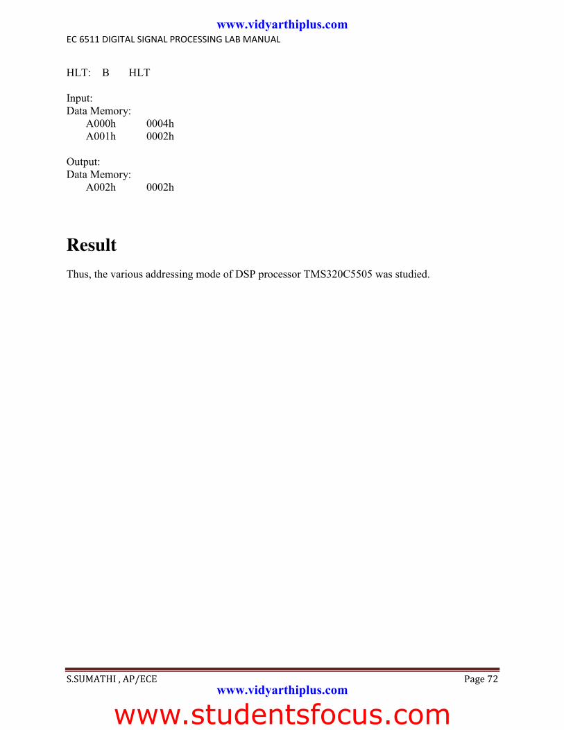
ADDITION INP1 .SET 0H INP2 .SET 1H OUT .SET 2H .mmregs .text START: LD #140H,DP RSBX CPL NOP NOP NOP NOP LD INP1,A ADD INP2,A STL A,OUT HLT: B HLT Input: Data Memory: A000h 0004h A001h 0004h Output: Data Memory: A002h 0008h SUBTRACTION INP1 .SET 0H INP2 .SET 1H OUT .SET 2H .mmregs .text START: LD #140H,DP RSBX CPL NOP NOP NOP NOP LD INP1,A SUB INP2,A STL A,OUT
www.vidyarthiplus.com
www.vidyarthiplus.com
www.studentsfocus.com
EC 6511 DIGITAL SIGNAL PROCESSING LAB MANUAL
S.SUMATHI , AP/ECE Page 72
HLT: B HLT Input: Data Memory: A000h 0004h A001h 0002h Output: Data Memory: A002h 0002h Result Thus, the various addressing mode of DSP processor TMS320C5505 was studied.
www.vidyarthiplus.com
www.vidyarthiplus.com
www.studentsfocus.com

EC 6511 DIGITAL SIGNAL PROCESSING LAB MANUAL
S.SUMATHI , AP/ECE Page 73
LINEAR CONVOLUTION AIM To perform the Linear Convolution of two given discrete sequence in TMS320C5505 KIT. REQUIREMENTS CCS v4 TMS320C5505 KIT USB Cable 5V Adapter THEORY Convolution is a formal mathematical operation, just as multiplication, addition, and integration. Addition takes two numbers and produces a third number, while convolution takes two signals and produces a third signal. Convolution is used in the mathematics of many fields, such as probability and statistics. In linear systems, convolution is used to describe the relationship between three signals of interest: the input signal, the impulse response, and the output signal.
If the input and impulse response of a system are x[n] and h[n] respectively, the convolution is given by the expression, x[n] * h[n] = ε x[k] h[n-k] Where k ranges between -∞ and ∞ If, x(n) is a M- point sequence h(n) is a N – point sequence then, y(n) is a (M+N-1) – point sequence. In this equation, x(k), h(n-k) and y(n) represent the input to and output from the system at time n. Here we could see that one of the inputs is shifted in time by a value every time it is multiplied with the other input signal. Linear Convolution is quite often used as a method of implementing filters of various types. Procedure
1. Open Code Composer Studio v4 . 2. In WorkSpace Launcher. Program:
www.vidyarthiplus.com
www.vidyarthiplus.com
www.studentsfocus.com

EC 6511 DIGITAL SIGNAL PROCESSING LAB MANUAL
S.SUMATHI , AP/ECE Page 74
.mmregs .text START: STM #40H,ST0 RSBX CPL RSBX FRCT NOP NOP NOP NOP STM #0A000H,AR0 ;AR0 for X(n) STM #00100H,AR1 ;AR1 for H(n) STM #0A020H,AR2 ;AR2 for temporary location ;temporary storage locations are initially zero LD #0H,A RPT #4H STL A,*AR2+ STM #0A004H,AR0 ;padding of zeros after x(n) LD #0H,A RPT #5H STL A,*AR0+ STM #0A000H,AR0 STM #0A020H,AR2 STM #0A030H,AR3 ;location for storing output Y(n) STM #6H,BRC ;counter for number of Y(n) RPTB CONV ;start of the program LD *AR0+,A STM #0A020H,AR2 STL A,*AR2 STM #0A023H,AR2 LD #0H,A RPT #3H MACD *AR2-,0100H,A CONV STL A,*AR3+ HLT: B HLT
www.vidyarthiplus.com
www.vidyarthiplus.com
www.studentsfocus.com

EC 6511 DIGITAL SIGNAL PROCESSING LAB MANUAL
S.SUMATHI , AP/ECE Page 75
INPUT: X(n) DATA MEMORY 0A000 0001H 0A001 0003H 0A002 0001H 0A003 0003H INPUT: H(n) PROGRAM MEMORY 00100 0000H ;h(n) 00101 0001H 00102 0002H 00103 0001H OUTPUT Y(n) DATA MEMORY 0A030 0001 0A031 0005 0A032 0008 0A034 0008 0A035 0007 0A036 0003
Result Thus, the Linear Convolution of two given discrete sequence has performed and the result is displayed .
www.vidyarthiplus.com
www.vidyarthiplus.com
www.studentsfocus.com
EC 6511 DIGITAL SIGNAL PROCESSING LAB MANUAL
S.SUMATHI , AP/ECE Page 76
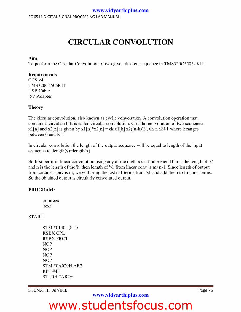
CIRCULAR CONVOLUTION
Aim To perform the Circular Convolution of two given discrete sequence in TMS320C5505s KIT. Requirements CCS v4 TMS320C5505KIT USB Cable 5V Adapter Theory The circular convolution, also known as cyclic convolution. A convolution operation that contains a circular shift is called circular convolution. Circular convolution of two sequences x1[n] and x2[n] is given by x1[n]*x2[n] = εk x1[k] x2((n-k))N, 0≤ n ≤N-1 where k ranges between 0 and N-1 In circular convolution the length of the output sequence will be equal to length of the input sequence ie. length(y)=length(x) So first perform linear convolution using any of the methods u find easier. If m is the length of 'x' and n is the length of the 'h' then length of 'yl' from linear conv is m+n-1. Since length of output from circular conv is m, we will bring the last n-1 terms from 'yl' and add them to first n-1 terms. So the obtained output is circularly convoluted output. PROGRAM: .mmregs .text START: STM #0140H,ST0 RSBX CPL RSBX FRCT NOP NOP NOP NOP STM #0A020H,AR2 RPT #4H ST #0H,*AR2+
www.vidyarthiplus.com
www.vidyarthiplus.com
www.studentsfocus.com

EC 6511 DIGITAL SIGNAL PROCESSING LAB MANUAL
S.SUMATHI , AP/ECE Page 77
STM #0A000H,AR0 ;x1(n) STM #0A010H,AR1 ;x2(n) STM #0A020H,AR2 STM #0A030H,AR3 ;output y(n) STM #3H,AR4 ;counter for finding y(1) to y(n) CALL ROT1 ;180 degree rotate for y(0) CALL CONV ;routine for convolution NEXTY:CALL ROT2 ;routine for 90 degree rotation CALL CONV BANZ NEXTY,*AR4- HLT: B HLT ;routine for 180 degree rotation ROT1: STM #0A011H,AR0 ;exchange x1(1) and x1(3) STM #0A013H,AR1 LD *AR0,A LD *AR1,B STL A,*AR1 STL B,*AR0 RET ;routine for 90 degree rotation ROT2: STM #0A013H,AR0 STM #0A012H,AR1 LD *AR0,A ;store x2(3) to acc(a)temporarily STM #2H,BRC RPTB ROT ;x2(2)->x2(3) LD *AR1-,B ;x2(1)->x2(2) ROT: STL B,*AR0- ;x2(0)->x2(1) STM #0A010H,AR0 ;acc(a)->x2(0) STL A,*AR0 STM #0H,BRC RET CONV: STM #0A000H,AR0 STM #0A010H,AR1 LD #0H,A
www.vidyarthiplus.com
www.vidyarthiplus.com
www.studentsfocus.com

EC 6511 DIGITAL SIGNAL PROCESSING LAB MANUAL
S.SUMATHI , AP/ECE Page 78
STM #3H,BRC RPTB CON LD *AR0+,T ;multiply and add loop CON: MAC *AR1+,A STL A,*AR3+ ;store the result in AR3 and increment AR3 RET INPUT X1(n) DATA MEMORY 0A000 0002 0A001 0001 0A002 0002 0A003 0001 INPUT X2(n) DATA MEMORY 0A010 0001 0A011 0002 0A012 0003 0A013 0004 OUTPUT Y(n) DATA MEMORY 0A030 000E 0A031 0010 0A032 000E 0A033 0010
Result Thus, the Circular Convolution of two given discrete sequence has performed and the result is displayed.
www.vidyarthiplus.com
www.vidyarthiplus.com
www.studentsfocus.com

EC 6511 DIGITAL SIGNAL PROCESSING LAB MANUAL
S.SUMATHI , AP/ECE Page 79
WAVE GENERATION Aim To Generate a Square waveform using TMS320C5505 DSP KIT. Requirements CCS v4 TMS320C5505 KIT USB Cable 5V Adapter Theory The simplest method to generate Sqaure wave is to use High Low concept for pin with delay. Square waves have an interesting mix of practice and theory. In practice, they are extremely simple. In their simplest form, they consist of an alternating sequence of amplitudes; e.g. high/low or 1's and 0's. The same high / low logic here we implented in experiment. For particular duration the high state is out , then low state is out. Finally square wave is generated and plotted in code composer studio Graph. PROCEDURE: 1. Download the program sin.asc in the prog. memory address 0h 2. Download the sine table values which is in the file datsine.asc in the program memory address 200h using PI 200h command in the XTALK.exe 3. Execute the program using GO 0 command. SINE WAVE GENERATION PROGRAM DESCRIPTION: The sine table values are stored in the program memory. Accumulator A is initially loaded with the starting address of the sine table. The read a instruction, reads the content of the address which is stored in acc. That data is sent to the DAC and the ACC. content is incremented to point to the next value in the sin table. PROGRAM DATA .SET 0H ADD .SET 1H TABLE .SET 200H .mmregs .text START: STM #140H,ST0 ;initialize the data page pointer
www.vidyarthiplus.com
www.vidyarthiplus.com
www.studentsfocus.com

EC 6511 DIGITAL SIGNAL PROCESSING LAB MANUAL
S.SUMATHI , AP/ECE Page 80
RSBX CPL ;make the processor to work using DP NOP NOP NOP NOP REP: LD #TABLE,A ;Load the address first value of the sine table to the accumulator STM #372,AR1 ;no. of sine table values LOOP: READA DATA ;read the sine table value PORTW DATA,04H ;send it to the dac ADD #1H,A ;increment the sine table address which ;is in the accumulator BANZ LOOP,*AR1- ;repeat the loop until all 372 values has been sent B REP ;repeat the above SQUARE WAVE GENERATION DATA .SET 0H .mmregs .text START: STM #140H,ST0 ;initialize the data page pointer RSBX CPL ;make the processor to work using DP NOP NOP NOP NOP REP: ST #0H,DATA ;send 0h to the dac CALL DELAY ;delay for some time ST #0FFFH,DATA ;send 0fffh to the dac CALL DELAY ;delay for some time B REP ;repeat the same DELAY: STM #0FFFH,AR1 DEL1: PORTW DATA,04H BANZ DEL1,*AR1- RET TRIANGULAR WAVE GENERATION DATA .SET 0H .mmregs .text
www.vidyarthiplus.com
www.vidyarthiplus.com
www.studentsfocus.com

EC 6511 DIGITAL SIGNAL PROCESSING LAB MANUAL
S.SUMATHI , AP/ECE Page 81
START: STM #140H,ST0 ;initialize the data page pointer RSBX CPL ;make the processor to work using DP NOP NOP NOP NOP REP: ST #0H,DATA ;initialize the value as 0h INC: LD DATA,A ;increment the value ADD #1H,A STL A,DATA PORTW DATA,04H ;send the value to the dac CMPM DATA,#0FFFH ;repeat the loop until the value becomes 0fffh BC INC,NTC DEC: LD DATA,A ;decrement the value SUB #1H,A STL A,DATA PORTW DATA,04H ;send the value to the dac CMPM DATA,#0H BC DEC,NTC ;repeat the loop until the value becomes 0h B REP ;repeat the above Result Thus, the Sine waveform ,Square waveform and Triangular waveform were generated and displayed at graph.
www.vidyarthiplus.com
www.vidyarthiplus.com
www.studentsfocus.com

EC 6511 DIGITAL SIGNAL PROCESSING LAB MANUAL
S.SUMATHI , AP/ECE Page 82
IMPLEMENTATION OF FIR FILTER Aim To Implement the FIR Low pass filter using TMS320C5505 KIT. Requirements CCS v4 TMS320C5505 KIT USB Cable 5V Adapter
Theory In signal processing, a finite impulse response (FIR) filter is a filter whose impulse response (or response to any finite length input) is of finite duration, because it settles to zero in finite time. This is in contrast to infinite impulse response (IIR) filters, which may have internal feedback and may continue to respond indefinitely (usually decaying). The impulse response of an Nth-order discrete-time FIR filter (i.e., with a Kronecker delta impulse input) lasts for N + 1 samples, and then settles to zero. For a discrete time FIR filter, the output is a weighted sum of the current and a finite number of previous values of the input. which defines the output sequence y[n] in terms of its input sequence x[n]:
Where, X(n) is input signal, y(n) is output signal and bi are the filter coefficients, also known as tap weights, that make up the impulse response. ;Filter type : Low pass filter
www.vidyarthiplus.com
www.vidyarthiplus.com
www.studentsfocus.com

EC 6511 DIGITAL SIGNAL PROCESSING LAB MANUAL
S.SUMATHI , AP/ECE Page 83
;Filter order : 2 ;Filter design type : Butterworth ;Pass band attenuation : 3db ;First corner freq : 0.2 ;Second corner freq : 0.24 ;Sampling freq : 50Khz ;Cut-off freq : 10Khz ; ;FROM PCDSP COEFFICIENTS ; XN .SET 0H XNM1 .SET 1H XNM2 .SET 2H YN .SET 3H YNM1 .SET 4H YNM2 .SET 5H XN1 .SET 6H XN1M1 .SET 7H XN1M2 .SET 8H YN1 .SET 9H YN1M1 .SET 0AH YN1M2 .SET 0BH TEMP .SET 0CH A10 .SET 0100H A11 .SET 0FFA2H A12 .SET 0032H B10 .SET 0100H B11 .SET 0200H B12 .SET 0100H PROGRAM: .mmregs .text START: STM #40H,PMST RSBX CPL STM #01H,ST0 RSBX FRCT
www.vidyarthiplus.com
www.vidyarthiplus.com
www.studentsfocus.com
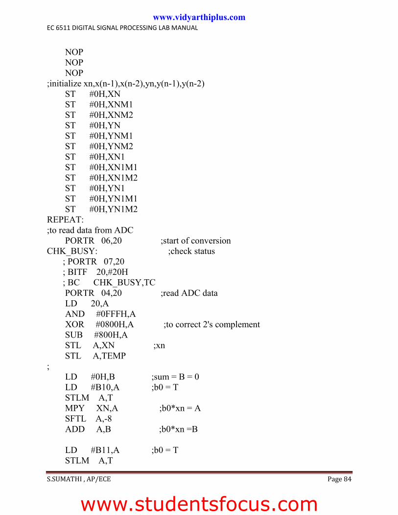
EC 6511 DIGITAL SIGNAL PROCESSING LAB MANUAL
S.SUMATHI , AP/ECE Page 84
NOP NOP NOP ;initialize xn,x(n-1),x(n-2),yn,y(n-1),y(n-2) ST #0H,XN ST #0H,XNM1 ST #0H,XNM2 ST #0H,YN ST #0H,YNM1 ST #0H,YNM2 ST #0H,XN1 ST #0H,XN1M1 ST #0H,XN1M2 ST #0H,YN1 ST #0H,YN1M1 ST #0H,YN1M2 REPEAT: ;to read data from ADC PORTR 06,20 ;start of conversion CHK_BUSY: ;check status ; PORTR 07,20 ; BITF 20,#20H ; BC CHK_BUSY,TC PORTR 04,20 ;read ADC data LD 20,A AND #0FFFH,A XOR #0800H,A ;to correct 2's complement SUB #800H,A STL A,XN ;xn STL A,TEMP ; LD #0H,B ;sum = B = 0 LD #B10,A ;b0 = T STLM A,T MPY XN,A ;b0*xn = A SFTL A,-8 ADD A,B ;b0*xn =B LD #B11,A ;b0 = T STLM A,T
www.vidyarthiplus.com
www.studentsfocus.com

EC 6511 DIGITAL SIGNAL PROCESSING LAB MANUAL
S.SUMATHI , AP/ECE Page 85
MPY XNM1,A ;b0*xn = A SFTL A,-8 ADD A,B ;b0*xn =B LD #B12,A ;b0 = T STLM A,T MPY XNM2,A ;b0*xn = A SFTL A,-8 ADD A,B ;b0*xn =B LD #A11,A ;b0 = T STLM A,T MPY YNM1,A ;b0*xn = A SFTL A,-8 SUB A,B ;b0*xn =B LD #A12,A ;b0 = T STLM A,T MPY YNM2,A ;b0*xn = A SFTL A,-8 SUB A,B ;b0*xn =B STL B,YN STL B,XN1 LD YNM1,A STL A,YNM2 LD YN,A STL A,YNM1 LD XNM1,A STL A,XNM2 LD XN,A STL A,XNM1 LD YN,A ADD #800H,A STL A,YN PORTW YN,04H B REPEAT HIGH PASS FIR FILTER
www.studentsfocus.com
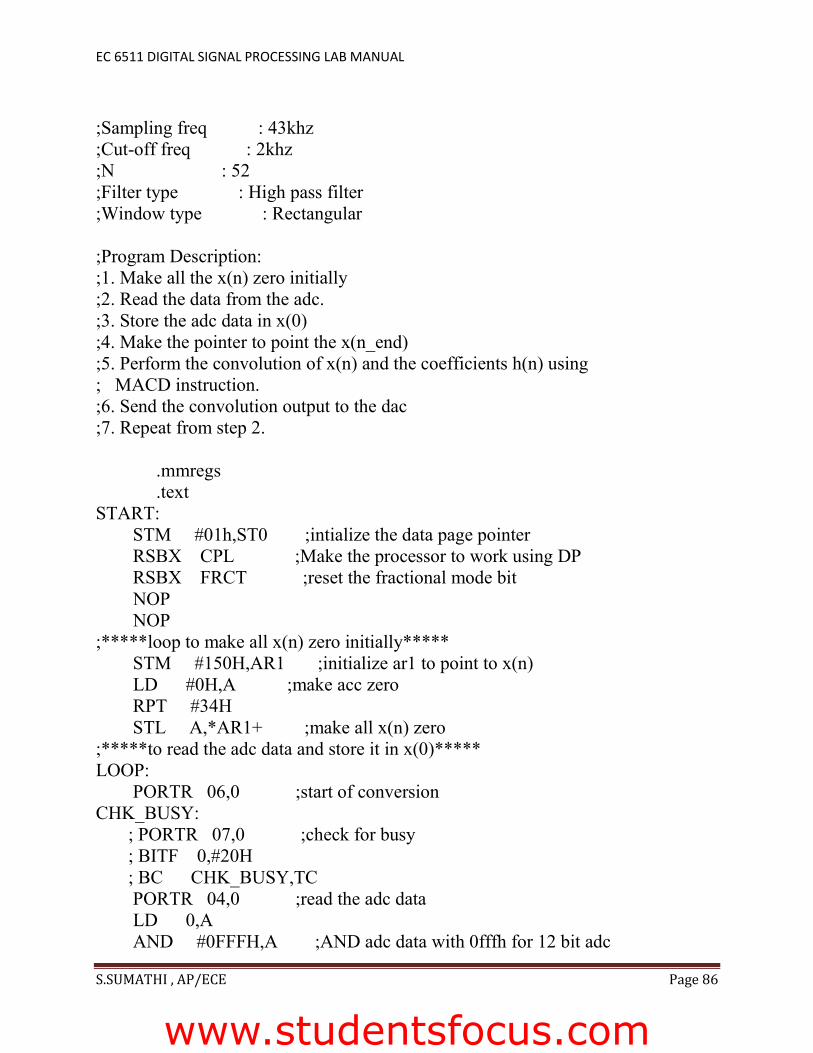
EC 6511 DIGITAL SIGNAL PROCESSING LAB MANUAL
S.SUMATHI , AP/ECE Page 86
;Sampling freq : 43khz ;Cut-off freq : 2khz ;N : 52 ;Filter type : High pass filter ;Window type : Rectangular ;Program Description: ;1. Make all the x(n) zero initially ;2. Read the data from the adc. ;3. Store the adc data in x(0) ;4. Make the pointer to point the x(n_end) ;5. Perform the convolution of x(n) and the coefficients h(n) using ; MACD instruction. ;6. Send the convolution output to the dac ;7. Repeat from step 2. .mmregs .text START: STM #01h,ST0 ;intialize the data page pointer RSBX CPL ;Make the processor to work using DP RSBX FRCT ;reset the fractional mode bit NOP NOP ;*****loop to make all x(n) zero initially***** STM #150H,AR1 ;initialize ar1 to point to x(n) LD #0H,A ;make acc zero RPT #34H STL A,*AR1+ ;make all x(n) zero ;*****to read the adc data and store it in x(0)***** LOOP: PORTR 06,0 ;start of conversion CHK_BUSY: ; PORTR 07,0 ;check for busy ; BITF 0,#20H ; BC CHK_BUSY,TC PORTR 04,0 ;read the adc data LD 0,A AND #0FFFH,A ;AND adc data with 0fffh for 12 bit adc
www.studentsfocus.com

EC 6511 DIGITAL SIGNAL PROCESSING LAB MANUAL
S.SUMATHI , AP/ECE Page 87
XOR #0800H,A ;recorrect the 2's complement adc data SUB #800H,A ;remove the dc shift STM #150H,AR1 ;initialize ar1 with x(0) STL A,*AR1 ;store adc data in x(0) STM #183H,AR2 ;initialize ar2 with x(n_end) ;*****start of convolution***** LD #0H,A ;sum is 0 initially RPT #33H MACD *AR2-,TABLE,A ;convolution process STH A,1,0H LD 0H,A ADD #800H,A ;add the dc shift to the convolution output STL A,1H PORTW 1H,04H ;send the output to the dac B LOOP TABLE: .word 0FCEFH .word 62H .word 0FD50H .word 14AH .word 0FE1BH .word 28FH .word 0FF11H .word 3E5H .word 0FFD1H .word 4ECH .word 0FFF5H .word 54FH .word 0FF28H .word 4DAH .word 0FD38H .word 398H .word 0FA2EH .word 1DDH .word 0F627H .word 55H .word 0F131H .word 4BH .word 0EA6DH .word 568H .word 0D950H .word 459EH .word 459EH .word 0D950H
www.studentsfocus.com

EC 6511 DIGITAL SIGNAL PROCESSING LAB MANUAL
S.SUMATHI , AP/ECE Page 88
.word 568H .word 0EA6DH .word 4BH .word 0F131H .word 55H .word 0F627H .word 1DDH .word 0FA2EH .word 398H .word 0FD38H .word 4DAH .word 0FF28H .word 54FH .word 0FFF5H .word 4ECH .word 0FFD1H .word 3E5H .word 0FF11H .word 28FH .word 0FE1BH .word 14AH .word 0FD50H .word 62H .word 0FCEFH
Result Thus, the FIR Low pass and High pass filter were Implemented and displayed the results in console window.
www.studentsfocus.com