ebooks for business students michael e. cafferky • jon
TRANSCRIPT

Breakeven AnalysisThe De� nitive Guide toCost-Volume-Pro� t AnalysisSecond Edition
Michael E. CafferkyJon Wentworth
Managerial Accounting CollectionKenneth A. Merchant, Editor
Breakeven AnalysisThe De� nitive Guide toCost-Volume-Pro� t Analysis, Second EditionMichael E. Cafferky • Jon WentworthThis second edition continues with the successful
comprehensive collection of cost-volume-pro� t ap-
plications. Whether you’re a business professional,
entrepreneur, business professor, or student, you will
bene� t from this one stop how-to book of formulas,
explanations, and examples. This new edition offers a
wide range of topics, from calculating basic breakeven,
to dealing with multiple products, mixed costs, chang-
ing costs, and changing prices.
Michael E. Cafferky is the Ruth McKee Chair for Entre-
preneurship and Business Ethics at Southern Adventist
University’s School of Business and Management. In an
addition to a doctoral degree in business from Anderson
University Falls School of Business he also holds mas-
ters degrees in public health and religion. The author
of eight books, Cafferky is a member of the Academy
of Management and the Christian Business Faculty As-
sociation. He has received Southern’s President’s Award
for Excellence in Scholarship and the national Sharon
Johnson Award from the Christian Business Faculty
Association.
Jon Wentworth is on the faculty of the School of
Business and Management at Southern Adventist Uni-
versity. He has received Southern’s Award for Commit-
ment to Student Success. He was previously the chair
of the accounting department at Klabat University in
Indonesia. He received an MBA from the University
of Tennessee and a Master of Taxation from Georgia
State University. He holds a Tennessee Certi� ed Public
Accountant license.
BREAK
EVEN
AN
ALY
SISC
AFFER
KY
• WEN
TW
OR
TH
Managerial Accounting CollectionKenneth A. Merchant, Editor
For further information, a free trial, or to order, contact:
[email protected]/librarians
THE BUSINESS EXPERT PRESSDIGITAL LIBRARIES
EBOOKS FOR BUSINESS STUDENTSCurriculum-oriented, born-digital books for advanced business students, written by academic thought leaders who translate real-world business experience into course readings and reference materials for students expecting to tackle management and leadership challenges during their professional careers.
POLICIES BUILT BY LIBRARIANS• Unlimited simultaneous
usage• Unrestricted downloading
and printing• Perpetual access for a
one-time fee• No platform or
maintenance fees• Free MARC records• No license to execute
The Digital Libraries are a comprehensive, cost-e� ective way to deliver practical treatments of important business issues to every student and faculty member.
ISBN: 978-1-63157-091-9
Breakeven Analysis


Breakeven Analysis
The Definitive Guide to Cost-Volume-Profit AnalysisSecond Edition
Michael E. Cafferky and Jon Wentworth

Breakeven Analysis: The Defi nitive Guide to Cost-Volume-Profi t Analysis, Second EditionCopyright © Business Expert Press, LLC, 2014.All rights reserved. No part of this publication may be reproduced, stored in a retrieval system, or transmitted in any form or by any means—electronic, mechanical, photocopy, recording, or any other except for brief quotations, not to exceed 400 words, without the prior permission of the publisher.
First published in 2010 byBusiness Expert Press, LLC222 East 46th Street, New York, NY 10017www.businessexpertpress.com
ISBN-13: 978-1-63157-091-9 (paperback)ISBN-13: 978-1-63157-092-6 (e-book)
Business Expert Press Managerial Accounting Collection
Collection ISSN: 2152-7113 (print)Collection ISSN: 2152-7121 (electronic)
Cover and interior design by Exeter Premedia Services Private Ltd, Chennai, India
First edition: 2010Second edition: 2014
10 9 8 7 6 5 4 3 2 1
Printed in the United States of America.

Abstract
This book is a comprehensive collection of cost-volume-profit applica-tions. Business professionals, entrepreneurs, business professors, and undergraduate and graduate business students will benefit from this one-stop how-to book of formulas, explanations, and examples. The user will find a wide range of topics, from calculating basic breakeven, to deal-ing with multiple products, mixed costs, changing costs, and changing prices.
Keywords
Annuity factor, breakeven (BE), cash flow, coefficient of determination, common stock dividend (CD), common stockholders, contribution mar-gin (CM), contribution margin ratio, cost of capital, cost of goods sold (COGS), cost-volume-profit (CVP) analysis, demand, fixed costs (FC), high-low method, income statement, income tax, least squares method, multiple regression, net present value (NPV), operating leverage, polyno-mial, preferred stock dividend (PD), preferred stockholders, price elastic-ity of demand, quadratic formula, scattergraph, target profit, total cost, total revenue, unit selling price (SP), unit variable costs (VC), weighted average contribution margin, weighted average selling price


Contents
Preface . . . . . . . . . . . . . . . . . . . . . . . . . . . . . . . . . . . . . . . . . . . . . . . ix
Chapter 1 Introduction . . . . . . . . . . . . . . . . . . . . . . . . . . . . . . . . . 1
Chapter 2 Total Cost Method . . . . . . . . . . . . . . . . . . . . . . . . . . . . 5
Chapter 3 Contribution Margin Method . . . . . . . . . . . . . . . . . . . 11
Chapter 4 Target Profit Method . . . . . . . . . . . . . . . . . . . . . . . . . . 17
Chapter 5 Cost of Goods Sold Method . . . . . . . . . . . . . . . . . . . . 21
Chapter 6 Modified Breakeven Analysis: Factoring Estimates of Demand . . . . . . . . . . . . . . . . . . 29
Chapter 7 Dealing With Changes in Product Mix Using Weighted Averages . . . . . . . . . . . . . . . . . . . 41
Chapter 8 High-Low Method. . . . . . . . . . . . . . . . . . . . . . . . . . . . 51
Chapter 9 Least Squares Method . . . . . . . . . . . . . . . . . . . . . . . . . 57
Chapter 10 Changing Costs . . . . . . . . . . . . . . . . . . . . . . . . . . . . . . 65
Chapter 11 Changing Prices . . . . . . . . . . . . . . . . . . . . . . . . . . . . . . 75
Chapter 12 Selling Price at Various Volumes . . . . . . . . . . . . . . . . . 85
Chapter 13 Multiple Breakeven Points . . . . . . . . . . . . . . . . . . . . . . 89
Chapter 14 Net Present Value Method . . . . . . . . . . . . . . . . . . . . . . 93
Chapter 15 Quadratic Equation . . . . . . . . . . . . . . . . . . . . . . . . . . 105
Chapter 16 Tax Effects on Cost-Volume-Profit . . . . . . . . . . . . . . . 115
Appendix A Glossary . . . . . . . . . . . . . . . . . . . . . . . . . . . . . . . . . . . 119
Appendix B Limitations and Criticisms . . . . . . . . . . . . . . . . . . . . . 127
Appendix C A Short Genealogy of Breakeven Analysis . . . . . . . . . 131

viii CONtENtS
Appendix D Using Breakeven Thinking to Decide Whether to Start a Business . . . . . . . . . . . . . . . . . . . . 135
Appendix E Annuity Table . . . . . . . . . . . . . . . . . . . . . . . . . . . . . . 141
Notes. . . . . . . . . . . . . . . . . . . . . . . . . . . . . . . . . . . . . . . . . . . . . . . . 143
References . . . . . . . . . . . . . . . . . . . . . . . . . . . . . . . . . . . . . . . . . . . . 147
Index . . . . . . . . . . . . . . . . . . . . . . . . . . . . . . . . . . . . . . . . . . . . . . . 153

Preface
Seldom does a manager go more than a month or two without employ-ing the thinking patterns that are at the foundation of this book. In some rapidly changing organizations, breakeven calculations will be used as fodder for discussions, debates, and ultimately decisions on a daily or weekly basis.
Today’s managers are far more sophisticated than those of a generation ago, but the need for cost-volume-profit thinking and breakeven decision-making tools has not gone away. Advances in cost accounting; the use of activity-based costing; the use of many performance-improvement tools such as identifying and removing constraints, optimizing logistics, and inventory management all lead down two interrelated pathways: value improvement and cost reduction.
Many existing companies have already picked the low-hanging fruit of performance improvement. With each passing year the gains from squeezing costs out of current systems become more and more difficult to achieve. These efforts have an impact on the breakeven point of the orga-nization. New companies, their managers learning fast from competitors, begin with the need to know where the breakeven point is. Breakeven thinking becomes second nature to seasoned managers who are faced with the ever-present need to fend off the onslaughts of competitors who are finding more efficient ways of doing business.
Who This Book Is Designed For
We start with the assumption that the users of this book will vary in their degrees of sophistication in terms of cost-volume-profit analysis. Some readers will have no business school background but have worked their way up to middle or senior management learning business concepts pri-marily in the context of their organization and industry. We take these readers from the basic concepts up through the advanced approaches. Some of these managers work in nonprofit organizations and government

x PrEFACE
agencies, which may not be attempting to achieve a profit but are nev-ertheless concerned about the prosperity of their organization. Many of these readers will have had no formal training in managerial accounting. We believe they will benefit from seeing this collection of tools. Practice and use of these tools will contribute toward these managers becoming more useful to their organizations.
Another group of users is entrepreneurs who, if they have been suc-cessful, have learned about breakeven thinking and analysis from their own experience. Many entrepreneurs don’t go to business school, pre-ferring to learn from their experiences in the market. This simple tool kit can bring into clear understanding much of what these entrepreneurs have been thinking about for a long time but didn’t have the range of tools readily available to do what they know needs to be done. As their enterprises grow and become more complex, they face the prospect of helping their top-level and midlevel management teams improve their thinking about the business. When dealing with suppliers and custom-ers, many of these entrepreneurs will improve their negotiating abilities by incorporating breakeven analysis into the negotiation process. Under-standing the breakeven point of your supplier and your customer can be just as valuable as knowing your own company’s breakeven point. In many negotiating situations the simple but effective tools discussed here provide insight and clarity, which can, if effectively presented, cut through the smoke and mirrors to the truth, revealing flaws or strengths in particular arguments.
Other users will have completed undergraduate business school and followed a career track that finds them in managerial positions. Most of these readers were exposed to one or two of the tools we present here. Still other readers will be MBA graduates who are at or heading toward senior-level leadership positions. Depending on the degree program they completed, they were exposed to one or more breakeven analysis tools in graduate school.
The last group of users will be undergraduate and graduate business students whose professors see value in exposing them to more than just one or two methods to calculate breakeven.

PrEFACE xi
The Plan of the Book
Think of this book as a ready-to-use managerial tool kit, which if used fre-quently will sharpen the manager’s ability to make decisions. We explain the vocabulary of breakeven analysis, also known as cost-volume-profit (CVP) analysis, explore the breadth of applications of CVP, and illustrate the use of CVP concepts in a broad range of management and marketing scenarios. While this book is not a comprehensive treatment of the topic, we employ many examples from several different types of industries to illustrate breakeven calculations.
The user of this book will find here a wide range of interrelated tools, from how to calculate basic breakeven to dealing with multiple products, mixed costs, changing conditions, and conditions of uncertainty. After an introductory chapter we present several commonly used breakeven analy-sis tools. With each tool we present one or more examples showing how the calculations work and the types of information needed for each one.
We hope this collection of practical tools will add value to your work as a manager regardless of where in the world of commerce, nonprofit, and government organizations you serve others.
Michael E. Cafferky and Jon WentworthSouthern Adventist University
Collegedale, Tennessee

Chapter 1
Introduction
Since its introduction in the 19th century, the breakeven concept has been used, enhanced, adjusted, and extended in an attempt to reduce or correct for its limitations and make it applicable to more and more business situations. In spite of its limitations and criticisms, detailed in Appendix B, breakeven analysis (also known as cost-volume-profit analysis) continues to be one of the best ways to focus on the relation-ship between cost, volume, and profitability. We present here the appli-cations and approaches that we believe managers will find most useful.
the essence of Breakeven analysis
Cost-volume-profit analysis is not just the mathematical result generated by applying a particular math formula. It is not merely a single num-ber used at a point in time, such as the number of units of a company’s products that it needs to produce and sell. In essence breakeven analy-sis is a continual way of thinking used by people potentially everywhere in the organization as they deal with a variety of decisions. As such it embraces the common ground of thinking that is used in accounting and economics.1
Overall breakeven thinking is a way of comparing the amount of incom-ing value that an organization needs in order to serve its customers by deliver-ing outgoing value of an equal amount. When applied to specific situations that might be changing, breakeven thinking is a way of comparing the impact of an anticipated change with the current situation. When these values can be quantified, a breakeven formula may be applied. But when values are intangible or unquantifiable, a mental comparison is still made.
2 Breakevenanalysis
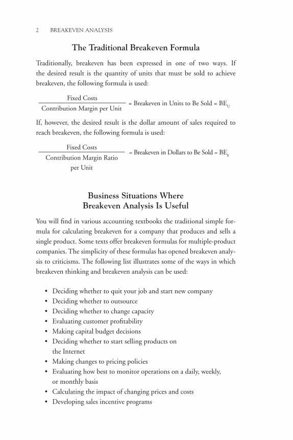
the traditional Breakeven Formula
Traditionally, breakeven has been expressed in one of two ways. If
the desired result is the quantity of units that must be sold to achieve
breakeven, the following formula is used:
Fixed Costs= Breakeven in Units to Be Sold = BE
UContribution Margin per Unit
If, however, the desired result is the dollar amount of sales required to
reach breakeven, the following formula is used:
Fixed Costs= Breakeven in Dollars to Be Sold = BE
$Contribution Margin Ratio
per Unit
Business Situations Where Breakeven analysis Is Useful
You will find in various accounting textbooks the traditional simple for-
mula for calculating breakeven for a company that produces and sells a
single product. Some texts offer breakeven formulas for multiple-product
companies. The simplicity of these formulas has opened breakeven analy-
sis to criticisms. The following list illustrates some of the ways in which
breakeven thinking and breakeven analysis can be used:
• Deciding whether to quit your job and start new company
• Deciding whether to outsource
• Deciding whether to change capacity
• Evaluating customer profitability
• Making capital budget decisions
• Deciding whether to start selling products on
the Internet
• Making changes to pricing policies
• Evaluating how best to monitor operations on a daily, weekly,
or monthly basis
• Calculating the impact of changing prices and costs
• Developing sales incentive programs

introduction 3
• Determining the minimum number of transactions to com-plete per day, per week, or per month
• Deciding to modify the composition of a product
Expressing breakeven thinking in terms of value will naturally lead us to consider the tangible, explicit values measured by cost and revenue. To this we turn next.


Chapter 2
total Cost Method
In this chapter we introduce the fundamental calculation that defines cost-volume-profit analysis from an accounting perspective. Let’s start with a short story.
Three managers at a manufacturing firm, Sharon Elsworth, Dante Jackson, and Larry Meeks, were having lunch together. After a couple of minutes of small talk, Dante said to the others, “Have you noticed that consumer demand is going through the roof for our product? Keep in mind that this is just a single-stage model. What no one is making, however, is a two-stage model. Haven’t you thought about that? I think about this so much I sometimes can’t get to sleep at night. It’s only a matter of time before someone will come out with the two-stager.”
Sharon said, “I’ve been so busy getting the bills paid and producing financial statements that I haven’t thought about a lot of things lately!”
Dante said, “I already talked with the big boss about this. He rejected the idea, saying that we need to stay with what we do best and ramp up our economies of scale more because there will come a day when the price will drop and we need to be prepared to weather the storm of heavier price competition. What do you think about the idea of us three working together, getting some investors together, and start-ing another production company?”
Larry said, “You’ve got to be kidding!”Dante replied, “I’m sure we could get approval from the board to
start another company. We wouldn’t have to quit our jobs right now. True, making a two-stager would be a little different from the model that is on the market now. But we know the basic operational side of this business. Think of the money we could make right now!”
The group began brainstorming and kicking around some numbers. Larry grabbed one of the paper napkins from the table and began jot-ting down figures. From the questions that surfaced around the table,

6 Breakevenanalysis
we can see that their minds were starting to evaluate the fundamental elements of a business model.
Sharon asked, “Do you really think this would work? What I want to know is how we will be able to pay our bills.”
Larry asked, “What will it take to make a profit? I don’t want to get into this unless there is an opportunity to make some money!”
Dante said, “True, we need to know that we will be able to get to breakeven, otherwise it won’t be worth it. We know the market price on the current model. If we made a two-stage model, it would sell at a price premium since it would offer more flexibility to users. At 500,000 units, which is just 5% of the demand of the current model, and a price that is 40% higher than the price point on the current model, pay attention! We are talking $10 million of total annual reve-nue here folks—$10 million!” He wrote this figure in large characters on the napkin.
Larry said, “True, but the costs of producing a two-stager would be higher, too. How do we know that we will be able to make this two-stage model, pay for the cost of running the business, and still break even?
Sharon reminded them, “What you are saying, Dante, is that we will be able to operate the business including the management, engi-neering, production, and a dynamite marketing team, and still pay for all the materials, packing, and other stuff for no more than $10 million. That is pretty aggressive given what we know about the production and marketing costs of the current model! I’d like to know what it would cost to make just one of these two-stagers, let alone 500,000 of them!”
What Sharon, Dante, and Larry are talking about is the first and most fundamental application of breakeven thinking.
One of the fundamental ways to apply breakeven analysis is by sim-ply thinking about the point where total revenue equals total costs for a defined period of time.1 This is one definition of the breakeven point.
Using the distinction between fixed costs (FC) and variable costs (VC), we can also say that we have reached the breakeven point when total revenue equals the sum of fixed costs and variable costs.

ToTalCosTMeThod 7
the Formula
Total Costs for Period = Total Revenue for Period = Breakeven
or
(Fixed Costs + Variable Costs) = Total Revenue = Breakeven.
Since total revenue equals the quantity sold times the unit selling price,
we can also extend this breakeven cost-to-revenue relationship with the
following formula:
(Fixed Costs + Variable Costs) =
(Quantity Sold × Unit Selling Price) = Breakeven.
example 1
The owner of Attashay Company develops the following data table for a
specific period:
Fixed Costs = $520,000
Variable Costs = $1,105,000
Total Costs = $1,625,000
The scale of costs represented here is different from that of many busi-
nesses. To make this and other examples in this book align with the scale
of operation in your situation, simply append to or remove zeros from
the total.
The following would be Attashay Company’s breakeven point for
the period:
($520,000 + $1,105,000) Total Costs =
$1,625,000 Total Revenue = Breakeven.
Interpreting the result
The breakeven amount is the dollar amount for the period that is spent
on operating expenses or generated in sales revenue. If you estimate the
total costs, you know what your total revenue must be and vice versa.

8 Breakevenanalysis
Users of this information will focus on one or the other side of the equation. For example, the accountant may be more interested in the total cost side, knowing the history or the expected future of revenue gen-eration. The marketing leader may likely be focused on the total revenue side of the equation as he or she thinks about the sales and marketing processes needed to cover expected costs.
Notice that although dollars are used to calculate the breakeven point, it is at this point that whatever number of units that have been produced and sold also is the breakeven in terms of units.
Depending on the type of business and the frequency with which this type of analysis helps in decision making, the relevant time period can be any common unit such as daily, weekly, monthly, quarterly, or annually. Annual total cost estimates can be broken down on a monthly basis and adjusted for known fluctuations in costs. Just recognize that as the time period increases in length, the presence of other influences on the change in costs and revenue will become greater.
This application of breakeven analysis looks at the business model’s big picture. It represents the overall magnitude of operations. Such an overview can be helpful when only generalized results are needed, and changes to the structure of fixed costs and variable costs are believed to be minimal. This broad-stroke approach can be useful as an initial approxi-mating method when details are not available. The big-picture approach also is less costly in terms of time and effort. However, since it takes such a broad view, it leaves undefined important details that, if known, could improve the precision of the breakeven calculation. One can think of this approach as yielding the crudest results.2
For some business situations, details on costs, revenue, or pricing may be difficult to obtain, such as in the early stages of planning for a new venture. The broad approach taken by this basic formula leaves out con-sideration of the number of units of the product or service that need to be produced and sold during the time period. It says nothing about the sales mix. Precise estimates of total costs and total revenue for a busi-ness operation may be difficult to determine in advance. Differentiating between fixed and variable costs may also be difficult.

ToTalCosTMeThod 9
extending the Formula
For some situations, if the company sells one product and if an estimate
of the going market price for that product is known and the decision
maker assumes that the company needs to match this market price, this
information can be used to estimate the number of units the company
needs to produce. The following example shows this calculation:
Total Costs = Quantity Sold × Unit Selling Price = Breakeven
Total Costs= Quantity Sold to Break Even
Unit Selling Price
So, for example, in Attashay Company if
Total Costs = $1,625,000
Unit Selling Price (Market Price) = $25
then the breakeven point is
$1,625,000 Total Costs= 465,000 Units Sold to Break Even.
$25 Unit Selling Price
Using an estimate of the market price conveys an important economic
assumption for the use of this formula for decision making. Company
managers are assuming that if the market price must be used in order
to be competitive, then customers will be highly responsive to changes
in price. The company and its competitors, under this situation, are left
with the prospect of competing not only on price but also correspond-
ingly on their relative abilities to lower their respective cost structures if
they expect to continue earning a profit.
Linking operational activities with the breakeven formula is vital
if you want to get the most value out of breakeven thinking. As we
will see in later chapters of this book, to be practical on a day-to-day
basis the breakeven amount expressed in either dollars or units must
be converted into a percentage of operational capacity. In the example
given previously, if company managers estimate that they will need to
produce and sell 465,000 units to break even, they must begin asking
themselves some serious questions, including the following:

10 Breakevenanalysis
• What is estimated capacity given our current cost structure? • What percentage of capacity must we use in order to achieve
the breakeven amount? • What kinds and amounts of hardware technologies will be
needed in order to provide the capacity required to break even? • Given a certain number of workdays per month, how many
units must be produced monthly? Weekly? Daily? • What configurations of employees, equipment, and other
resources will be needed on a daily basis to achieve breakeven? • If we are constrained by fixed capacity, what additional fixed
costs will be incurred to bring capacity up to a level where we can break even? How will these additional fixed costs change the breakeven point?
• What level of intensity must sales and marketing activities employ in order to stimulate demand sufficient to break even?
Think of the total cost method as the first opportunity to test your assumptions about the market and about your company’s ability to meet market needs. To the degree that your assumptions are accurate, the big picture of your company’s business model will be an accurate reflection of what the company and every department in it needs to do daily.
additional application
This basic formula uses summary data from an income statement. But the same principle can be applied when using data from the statement of cash flows as follows:
Total Cash In = Total Cash Out = Breakeven Point for Period.
This formula can be applied to a portion of the statement of cash flows, such as just the cash flows from operations or just the cash flows from investments.
The extension of this basic formula leads us naturally to think about the other approaches to breakeven analysis. To these we turn next.

Chapter 3
Contribution Margin Method
The basic approach to the breakeven calculation is the contribution mar-gin method. This method is a refinement of the total cost method. This method, which indicates the number of units that must be produced and sold, is particularly useful to people involved in the acquisition of raw material and labor, actual production of the finished product, and storage and shipping of the product. The resulting target value of units to be pro-duced and sold will guide many of the departmental functions of a com-pany. The number of units required to meet the target focuses the production side of the company on how much work must be done. The purchasing department will base materials purchases on “the number.” Human resources will decide how many employees are needed; the production manager will decide how to schedule production runs and work shifts; the warehouse manager will gauge how much storage space is needed; and the transportation department will arrange for adequate contain-ers, trucks and trailers, or rail cars to handle the volume of goods to be shipped.
To apply this method, the user needs to know the selling price per unit, the variable cost per unit, and the total fixed costs for the period being analyzed. Contribution margin (CM) is the difference between rev-enues and variable costs. Recall that the contribution margin is calculated as the selling price per unit less the variable cost per unit. The contri-bution margin tells you that after the variable costs have been covered, each unit of product or service sold to the customer contributes a certain amount toward paying for fixed costs.
The contribution margin method expresses breakeven as
Fixed Costs= Breakeven in Units to Be Sold.
Contribution Margin per Unit
12 Breakevenanalysis
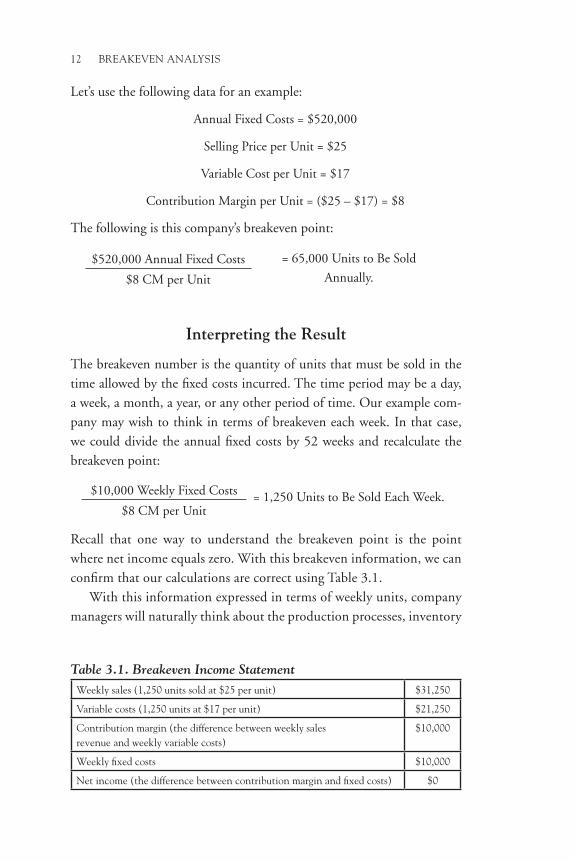
Let’s use the following data for an example:
Annual Fixed Costs = $520,000
Selling Price per Unit = $25
Variable Cost per Unit = $17
Contribution Margin per Unit = ($25 – $17) = $8
The following is this company’s breakeven point:
$520,000 Annual Fixed Costs = 65,000 Units to Be Sold
Annually.$8 CM per Unit
Interpreting the result
The breakeven number is the quantity of units that must be sold in the time allowed by the fixed costs incurred. The time period may be a day, a week, a month, a year, or any other period of time. Our example com-pany may wish to think in terms of breakeven each week. In that case, we could divide the annual fixed costs by 52 weeks and recalculate the breakeven point:
$10,000 Weekly Fixed Costs = 1,250 Units to Be Sold Each Week.$8 CM per Unit
Recall that one way to understand the breakeven point is the point where net income equals zero. With this breakeven information, we can confirm that our calculations are correct using Table 3.1.
With this information expressed in terms of weekly units, company managers will naturally think about the production processes, inventory
Table 3.1. Breakeven Income StatementWeeklysales(1,250unitssoldat$25perunit) $31,250
variablecosts(1,250unitsat$17perunit) $21,250
Contributionmargin(thedifferencebetweenweeklysalesrevenueandweeklyvariablecosts)
$10,000
Weeklyfixedcosts $10,000
netincome(thedifferencebetweencontributionmarginandfixedcosts) $0
ContriButionMarginMethod 13
management, support equipment, and other resources that need to be
in place and used consistently. Support departments will be organized
around the production departments, which are organized around the
production goals. Sales and marketing personnel will begin thinking
about the kinds of activities needed to stimulate demand. Managers will
take into consideration any seasonality to patterns of demand. Financial
managers will think about the amount of working capital (cash) needed
to support the operations.
extending the Formula: the Contribution Margin ratio Method
As stated previously, certain users need information stated in units.
Other users are “top line” driven and need to know the breakeven point
in sales dollars instead of units to be sold. The sales dollars necessary
to meet the target focuses the marketing side of the company on how
much work must be done. These users would plan how many contacts
must be made with prospective customers, how many deals must be
closed or transactions completed, how many sales representatives must
be hired to make those contacts, the sales travel-expense budget, the
type and quantity of promotional efforts, and the budget for sales com-
missions for the coming year.
One advantage of the contribution margin ratio method over the
basic contribution margin method is that the ratio method can be applied
whether the number of units is known or unknown, since the ratio can
be obtained from per unit amounts or from total amounts.
If the breakeven point in units is already known, then the breakeven
point in sales dollars would be calculated as selling price per unit times
breakeven sales units. Continuing with the annual data from the pre-
ceding example, the breakeven point in sales dollars would be
65,000 Units to Be Sold × $25 Selling Price per Unit = $1,625,000.
If the breakeven point in units is not already known, then the breakeven
point in sales dollars could be calculated directly:
Fixed Costs = Breakeven in Sales DollarsContribution Margin Ratio

14 Breakevenanalysis
The contribution margin ratio (CM ratio) expressed as a percentage is
calculated:
Contribution Margin per Unit= CM Ratio.
Selling Price per Unit
Applying our previous per unit data, the CM ratio would be
$8 CM per Unit= 0.32 or 32%.
$25 Selling Price per Unit
The CM ratio may also be calculated:
Total Contribution Margin= CM Ratio.
Total Revenue
For illustration’s sake, let’s assume the company sells 70,000 units annu-
ally. Applying our previous data using total amounts, the contribution
margin would be
Total CM ($8 per Unit × 70,000 Units)= 32% CM Ratio.
Total Revenue ($25 × 70,000 Units)
The choice between calculating the contribution margin ratio with per
unit amounts and calculating the ratio with total amounts depends on
the data available to the user.
Recall that the annual fixed costs were $520,000. So the breakeven in
sales dollars would be
$520,000 Annual Fixed Costs= $1,625,000 to Be Sold Annually.
0.32 CM Ratio
The CM ratio method can be applied to various time periods (weekly,
monthly, or quarterly, for example), just as with the CM method. Let’s
see how much the sales budget must be for one week, using our previous
weekly data.
$10,000 Weekly Fixed Costs = $31,250 to Be Sold Each
Week.0.32 CM Ratio
We can check that sales target by multiplying the breakeven sales units by
the unit selling price:

ContriButionMarginMethod 15
1,250 Units × $25 Selling Price per Unit = $31,250.
In alternate settings, the contribution margin may be calculated on a
product line, a division producing multiple products, a customer, or a
sales region.
a Few Notes on Operating Leverage
While the subject of operating leverage deserves more attention than we
can give it in a book focused just on breakeven analysis, a few notes are
appropriate.
Something interesting to observe with the contribution margin
method is the effect on the breakeven point of fixed costs and of variable
costs. As fixed costs increase, the breakeven point increases and the profit
potential of the organization goes up with increased volume of sales. But
if the sales level (demand) drops, the company will have difficulty in pay-
ing its fixed costs and the loss potential also goes up. For companies that
face an uncertain or widely fluctuating demand, keeping fixed costs low
minimizes the risks that come with fixed costs. This is one reason we see
entrepreneurs keeping the fixed costs of their businesses low until they get
established. As unit variable costs increase, the breakeven point increases
and of course the profit potential goes down. As the ratio of fixed costs
to variable costs increases, we say that the company’s operating leverage
increases since a small percent change in sales will lead to a large percent
change in operating profit. The formula that is usually employed to cal-
culate operating leverage is as follows:
Operating Leverage = % Change in Earnings Before Interest and
Taxes ÷ % Change in Sales.
The following is the shorthand version of the formula:
OL = %zEBIT ÷ %DSales,
where
%DEBIT = % Change in Earnings Before Interest and Taxes
%DSales = Percent Change in Sales.

16 Breakevenanalysis
Organizations have varying degrees of choice regarding the amount of fixed costs and the amount of variable costs to incur. For example, a com-pany in one industry may have the option of purchasing a new piece of equipment that will improve the efficiency of production (lower the variable costs per unit) while at the same time increasing fixed costs such as paying for routine maintenance or utility costs. A company in another industry, because of the nature of the business, may not have this flexibil-ity. Companies that offer services typically have very high fixed costs and low variable costs. The attractiveness of the profits from services entices entrepreneurs to start service businesses, but the volatility of sales can make new service businesses more risky because of the high fixed costs.
The concept of contribution margin is helpful in many applications of breakeven thinking. We will consider some of these starting with the next chapter: calculating breakeven to achieve a target profit.

Chapter 4
target profit Method
While knowing the breakeven point is useful information, the objective of every business is to go beyond breakeven and achieve a profit. We can incor-porate the target profit of the business into the breakeven formula in one of two ways.
Management may set a fixed amount of desired profit for the period (month, quarter, or year). That fixed desired profit is treated as an additional fixed cost in the formula.
Fixed Costs + Desired Profit=
Units to Be Sold to
Achieve Desired ProfitContribution Margin (CM) per Unit
Let’s continue using the data from the example in the preceding chapter and add a desired profit of $52,000 per year.
Annual Fixed Costs = $520,000
Selling Price per Unit = $25
Variable Cost per Unit = $17
Contribution Margin per Unit = $8
Annual Desired Profit = $52,000
Including the desired profit in the equation, the breakeven point is as follows:
$520,000 Annual Fixed Costs +
$52,000 Desired Profit =71,500 Units to Be
Sold Annually.$8 Contribution Margin per Unit
If management wants to set a weekly sales target, the calculation would be

18 Breakevenanalysis
$10,000 Weekly Fixed Costs + $1,000
Weekly Desired Profit =137.5 Units to Be
Sold Each Week.$8 Contribution Margin per Unit
While mathematically correct, our solution for the weekly sales target
presents a problem. Customers generally buy complete products, not
fractional portions of products. To resolve this problem, simply round
any fractional unit up to the next higher whole unit. Our sales target per
week would be 138 units.
As with the basic breakeven calculation, we can calculate the sales dol-
lars required to reach the desired profit:
$520,000 Annual Fixed Costs +
$52,000 Desired Profit=
$1,787,500 to be
Sold Annually0.32 CM Ratio ($8 ÷ $25)
or
71,500 Units Sold Annually × $25 Selling Price per Unit =
$1,787,500 Annual Sales.
Alternatively, management might express its profit objective as an amount
per unit of sales, a variable target profit. The formula would be modified
this way:
Fixed Costs=
Units to Be Sold to
Achieve Desired Profit.Contribution Margin per
Unit – Desired Profit per Unit
Here again are our data:
Annual Fixed Costs = $520,000
Selling Price per Unit = $25
Variable Cost per Unit = $17
Contribution Margin per Unit = $8
Desired Profit per Unit = $2

TargeTProfiTMeThod 19
$520,000 Annual Fixed Costs=
86,666.67 Units to Be
Sold Annually.$8 CM per Unit – $2 Desired
Profit per Unit
And, as before, the fractional unit would be rounded up, so the sales tar-
get is 86,667 units.
If management wanted to see the weekly sales target in units, we
would calculate it like this:
$10,000 Weekly Fixed Costs=
1,666.67 Units to Be
Sold Each Week.$8 CM per Unit – $2 Desired
Profit per Unit
This rounds up to 1,667 units sold per week.
Again, the sales dollars required to achieve the target profit can be
calculated. First, we need to recalculate the contribution margin ratio:
$6 ÷ $25 = 0.24 or 24%.
Then calculate the annual sales dollars needed:
$520,000 Annual Fixed Costs=
$2,166,667 (rounded)
to Be Sold Annually.0.24 CM Ratio
A refined approach to applying the target profit method was suggested by
Bell.1 Instead of using a single value for desired profit, he suggested that
preferred stock and common stock dividends be added to the fixed costs.
Under this approach, our formula would be
Fixed Costs + Preferred Stock Divi-
dend + Common Stock Dividend +
Desired Profit = Breakeven.Contribution Margin per Unit
Using the data from the beginning of this chapter and adding dividend
information, the calculation works out like this:
Annual Fixed Costs (FC) = $520,000
Selling Price per Unit = $25
Variable Cost per Unit = $17
Contribution Margin per Unit (CM) = $8

20 Breakevenanalysis
Annual desired profit to be retained by the company (RE) = $52,000
Dividends to be paid to preferred stockholders (PD) = $13,000
Dividends to be paid to common stockholders (CD) = $20,000
$520,000 FC + $52,000 RE +
$13,000 PD + $20,000 CD=
75,625 Units to Be
Sold Annually.$8 CM per Unit
Ideally, contribution margin is identified using selling price and variable costs. When variable cost data are difficult to get, we need an alternative approach. The cost of goods sold method is one such approach, to which we turn next.

Chapter 5
Cost of Goods Sold Method
In situations where the volume of different products makes the tradi-tional approach impractical, the cost of goods sold (COGS) method1 may be more appropriate. For example, you operate a restaurant that offers a large number of menu selections to customers. Calculating the unit vari-able cost for each menu item might be difficult when many ingredients are used in small amounts for each item sold. The selling price of each menu item is known, but the combination of menu items that each cus-tomer selects is highly variable, making the job of calculating the unit selling price very difficult. Over time we may be able to develop some rules of thumb for average per-customer revenue for different times of day and different seasons of the year. Using averages will likely reduce the precision of our estimate. Thus, calculating the breakeven point for each menu item would likely be impractical.
the Formula
The basic breakeven relationships still apply, such as the fact that your restaurant incurs fixed costs and there is a potential for each meal served to provide a contribution margin (CM) toward covering fixed costs.
Breakeven (in dollars) = Fixed Costs ÷ Contribution Margin %
The first task is to identify which of the expense items on the income statement represent fixed costs. The next step is to identify the contribu-tion margin.
example 1
Table 5.1 is an example from a simplified income statement (also known as a profit and loss statement or P&L).

22 Breakevenanalysis
Using the breakeven formula, BE = Fixed Costs ÷ Contribution Margin Ratio, we can calculate the breakeven point in dollars like this:
BE = FC ÷ CM%
BE = $292,000 ÷ 0.454
BE = $642,962.
Interpreting the result
In our hypothetical restaurant we must sell at least $642,962 (or round-ing it up to a nice round figure $643,000) during the relevant period to break even. Some restaurants earn far more than this. When the overall economy slumps, revenue in the full-service restaurant indus-try also declines as more people decide to eat at home. Changing eco-nomic conditions are all the more reason to monitor breakeven point and make adjustments as needed. Restaurants that are in the middle of the industry in terms of average check per customer are getting profits squeezed as competitive rivalry increases in the market segments below and above them. Another economic dimension that adds to the ratio-nale for monitoring breakeven in this particular industry is that even in a strong economy the overall growth rate of demand is low. Competi-tion for the restaurant dollar can be intense in some markets.
Fixed costs for a restaurant include marketing expenses, manager’s salary and benefits, general administrative expenses, telephone, Internet, cable TV, interest, licenses, bank charges, utilities, repairs, insurance,
Table 5.1. Simplified Income Statement
as a % of gross revenueGrossrevenue $687,000 100%
Costofgoodssold $350,000
Grossprofit $337,000
Othervariablecosts $25,000
Contributionmargin $312,000 45.4%
Fixedcosts $292,000
Pretaxprofit $20,000 2.9%

COstOFGOOdssOldMethOd 23
occupancy costs such as rent, maintenance, janitorial services, depre-ciation, and other operating expenses. In some restaurants music and entertainment might be considered fixed costs. In other restaurants these might be variable costs.
For most restaurants variable costs include not only the cost of food and beverage products (COGS), since these vary directly with the vol-ume of customers served, but also the cost of direct labor and benefits represented by servers, server helpers, cooks, hosts, temporary work-ers, and shift managers. Franchise royalties are also a variable cost since these normally are tied to the volume of sales. Table coverings and place settings may be variable costs. If paper goods are used, these are dispos-able and therefore constitute a variable cost. If linen is used, laundry expenses are incurred. The number of employees also represents a lim-ited capacity for sales. Delivery drivers and fuel costs also can be a variable expense. Employee time cards and the payroll system can be coded to reflect the variable cost nature of direct labor and benefits. This is important since it allows the manager to distinguish between fixed costs and variable costs.
Contribution margin in dollars is calculated as the difference between gross revenue and total variable costs. Contribution margin can then be estimated as a percentage of gross revenue. To calculate the CM percentage we start with gross revenue, subtract the cost of goods sold, and subtract the other variable costs. We then divide the remain-der by the gross revenue.
To get this information readily, an important consideration for any business—including a restaurant—is the structure of the chart of accounts for the general ledger. Most accounting systems are structured to meet obligations to the Internal Revenue Service (IRS), which is good except that the IRS obligations do not, by themselves, consider the information needed to monitor a firm’s breakeven point. Gener-ally accepted accounting principles (GAAP) encourage accountants to structure the accounting information system so that auditing is transparent and straightforward. Sometimes the accounting system fails to take into consideration whether the structure of the account-ing information supports breakeven analysis or not. If fixed costs and variable costs are difficult to identify, calculating the breakeven point is more difficult.

24 Breakevenanalysis
Here’s an example of a small portion of a chart of accounts used to monitor revenue derived from the sale of food:
• Sales of food—retail
Rolled into this one line item may be a lot of detail. For example, notice the difference between this item and the following list that divides the revenue by meal period and category of food:
• Entree sales breakfast • Entree sales breakfast takeout • Beverage sales breakfast • Beverage sales breakfast takeout • Dessert sales breakfast • Dessert sales breakfast takeout • Entree sales lunch • Entree sales lunch takeout • Beverage sales lunch (nonalcoholic) • Beverage sales lunch takeout (nonalcoholic) • Salad sales lunch • Salad sales lunch takeout • Dessert sales lunch • Dessert sales lunch takeout • Entree sales dinner • Entree sales dinner takeout • Beverage sales dinner • Beverage sales dinner takeout • Salad sales dinner • Salad sales dinner takeout • Dessert sales dinner • Dessert sales dinner takeout • Liquor sales lunch • Beer sales lunch • Wine sales lunch • Liquor sales dinner • Beer sales dinner • Wine sales dinner

COstOFGOOdssOldMethOd 25
A level of detail can be added for classifying sales by location (dining room, coffee shop, grill, patio, drive-through, banquets) if this is relevant to what the restaurant offers. With the chart of accounts structured this way, information can be aggregated by mealtime or by product category. Most computerized cash register systems available these days can handle this level of detail. Of course, depending on the type of restaurant there might be other revenue streams such as souvenirs or sale of food at catered events. The point here is that the business owner can make an informed judgment about the level of detail to capture for analysis.
Cost of goods sold can also be expanded to include the various cat-egories of food products and labor expenses. For example, the following might be used in one segment of the chart of accounts:
• Food costs—entrees • Food costs—beverages • Food costs—salads • Food costs—desserts • Carryout supplies • Linen • Paper/disposables
Direct labor can be classified according to the meal period worked.Having good information is vital. For example, a restaurant owner
may choose to provide an incentive for servers to promote a particular type of menu item that offers a good contribution margin. Traditionally, desserts are high-profit items in full-service restaurants. Incentives can change the product mix of an organization, shifting the breakeven point up or down. But without adequate information about the breakeven point, the incentive system may inadvertently incentivize employee behavior that undermines profitability.
Benefits
Several benefits to the COGS approach can be noted.2 One of the ben-efits of this approach is that the data comes right from the income state-ment. An income statement can be produced on a monthly basis. It is a report that is readily available. No new data needs to be developed to
26 Breakevenanalysis
use this method, and the information is aggregated over a relevant time period. This approach gives the restaurant owner an overall target of gross revenue to shoot for.
Sales dollars is the most common element of measure in any busi-ness. Sooner or later all productive work and production measures will be converted to sales dollars. Sales binds together the breakeven point and the income statement.
If we know (or expect) a certain proportion of our gross revenue will be generated by serving breakfast, another proportion by serving lunch, and another proportion by serving dinner, we can set some sales targets for the restaurant for these three mealtimes. For example, we might determine that in our market we generate 20% of our rev-enue at breakfast ($128,600), 30% at lunch ($192,900), and 50% at dinner ($321,500). We can set sales targets and design marketing promotional campaigns accordingly. Like all restaurants do, we will work vigorously to fine-tune the labor portion of the fixed costs for the three mealtimes.
We can break down the breakeven revenue on a per-day and per-meal-period basis. At this point we might want to employ our knowl-edge of the average per-plate revenue at breakfast, at lunch, and at dinner. Such information can then be used to estimate the number of customers we must serve at breakfast, lunch, and dinner to break even and the number of support staff needed to accomplish this. Informing employees of this can help them understand the reason behind the need to serve customers in a timely manner, clean up, and prepare for serving more customers at each mealtime.
For example, if we estimate that the average per-plate revenue at breakfast is $7.25, we will need to serve 1,187 breakfast customers during the relevant period of time. If the average per-plate revenue at lunch is $9.50, we will need to serve 2,030 lunch customers. If the aver-age per-plate revenue at dinner is $15.75, we will need to serve 2,041 customers at dinner. Naturally, we will review the amount of seating space in the restaurant to make sure that our capacity can adequately serve this number of people.
Another way a restaurant can analyze the operational impact on breakeven is by the traditional categories of beverages, salads, entrees, and desserts, meaning by product category rather than by the type

COstOFGOOdssOldMethOd 27
of meal served. With close analysis the contribution margin of each product category can be estimated. The operational ability to prepare and serve each category of food is at the core of the business.
Breakeven thinking can be extended into the operations in this type of business by considering the mix of tables or service areas pro-vided. For example, if your restaurant only has booths seating six peo-ple each, and you have 20 booths, you could be limiting your ability to break even since a single customer coming in will tie up a whole booth. Having a mix of tables allows for groups of different sizes to eat at the restaurant.3
Limitations
Like all methods of estimating breakeven, this approach has its limita-tions. The cost of goods sold method, like other methods, depends on having accurate historical information. It is retrospective in its perspective. Using this approach to look to the future to estimate the breakeven point depends heavily on your assumptions. If you are using assump-tions based on recent past history, you must assume future consumer behavior will continue relatively unchanged into the immediate future (into the next relevant, short-term period of time for which breakeven needs to be estimated). This method calculates breakeven in terms of dollars of gross revenue but not the number of units sold. We can estimate the number of units sold (customers served) to break even, but such an estimate will have a margin of error that is unacceptable in a highly price-competitive market where customers are more price sensitive.
For every business that sells more than one product or service, the issue of sales mix or product mix affects the breakeven point. The broad COGS approach does not attempt to take into account the sales mix. For some businesses, the fluctuation in sales mix from day to day or week to week can be great. This variation has a direct impact on the variability of the breakeven point. The greater the variability of the break-even point, the greater the risk that managers will not have the informa-tion needed to make timely decisions as conditions change.
By itself, the cost of goods sold approach does not tell you how the breakeven point changes with volume of sales or as the scale

28 Breakevenanalysis
of capacity changes. This reflects a related weakness of the COGS approach: it can be seen as superficial and lacks a level of detail to pro-vide alert management with good information to control profitability.
Although sales dollars is the most common element tracked by a business, the sales dollar cannot be applied with ease to all depart-ments. For example, maintenance and janitorial services are only indi-rectly linked with sales dollars. This doesn’t mean that the cleanliness and operational effectiveness of a restaurant are unimportant for gen-erating sales. Indeed, cleanliness is one of the reasons customers will come back to a restaurant.

Chapter 6
Modified Breakeven analysisFactoring Estimates of Demand
We know selling price plays an important part in determining the break-even point. With everything else unchanged, the lower the price, the higher the breakeven point and vice versa. Cost is an important factor that influ-ences price. In fact, we can say that price is never completely separated from cost considerations. With everything else unchanged, the higher the costs the more managers will be inclined to raise the price and vice versa. Price in its relationship to cost is important, but it is not the only factor to consider.
For most products and services offered in competitive markets, manag-ers must take into consideration the competition and how customer behav-iors might change if the price changes. For some products a small percent increase in price can make a significant difference in whether the company is able to break even. But what impact will increasing the price have on cus-tomers’ willingness to buy when substitute products are readily available? In other words, how will demand change if the price changes?
The traditional breakeven formula is a cost-based approach. It is silent regarding the influence of demand on breakeven. In this chapter we will review a modified breakeven analysis method that factors in estimates of demand.1 To do this we will first review the basic idea of demand.We will then review some approaches to estimating demand and customer responsiveness to price changes. Finally, we will see how to use estimates of demand to calculate the breakeven point and in the process find the “sweet spot” of optimal profit.
Demand
Demand is an estimate of the volume of a product or service that customers are willing to buy at different levels of price.2 For most products and ser-vices, if the price falls, we expect that customers are more willing and able to purchase a higher quantity than they would otherwise purchase.

30 BrEakEvEn analysis
Visually we represent this price-demand relationship (Figure 6.1) with a downward-sloping line on a graph where price is on the vertical axis and quantity demanded is on the horizontal axis.
Demand is driven by several factors: consumer tastes, the number of buyers in the market, income, prices of substitutes and complementary goods, and customer expectations. For example, in the early 1980s when people began to see the power of personal computers (PCs), consumer tastes began to shift away from the use of typewriters. This occurred even though at the time the electric typewriters used in most businesses were becoming sophisticated enough to help the typist correct errors. Printers had not yet developed to the point where letter-quality printing could be created on the same page as graphics. Over a period of just a few years, demand for electric typewriters began to shift and all but die out as demand for PCs dramatically increased. This became a shift in the demand curves of both typewriters and personal computers. Using Figure 6.1, the demand curve for typewriters began to shift to the left as the demand curve for per-sonal computers began to shift to the right.
As managers saw the power of personal computers and software appli-cations were developed to increase efficiency, most companies were will-ing and able to purchase at least one personal computer. But as workers began to envision how the personal computer could make their work more efficient, interest began to grow and company managers were more willing to spend money on this product. As the price of PCs began to
1 2 4 50
2
4
6
8
10
12
Pric
e
Quantity Demanded
Demand
Figure 6.1. Price-Demand Relationship

MoDiFiED BrEakEvEn analysis 31
drop, companies were willing and able to buy more PCs. This became movement along the demand curve.
The question managers had to deal with was this: If the price changed, how responsive would customers be in terms of their willingness and ability to purchase a personal computer? As with most products and services, the presence of readily available substitute products is the primary influence on customer responsiveness to price changes.3 We sometimes talk about respon-siveness to price changes in terms of price elasticity of demand. If there are few readily available substitutes and customers want the product, producers can increase the price and customers will continue in their willingness to purchase. In contrast, if there are many readily available substitute products and customers want the product, producers who increase the price will find that customers will switch to a substitute. Another way of seeing this is to say that if companies are unable or unwilling to make their product different from substitute products along the lines that customers find important, then price becomes more important to customers and they are more willing to stop buying the higher priced product in favor of the lower priced product.
Recall that the breakeven point is the point at which total revenue equals total costs. The impact of customer responsiveness on total revenue is important. When prices increase and customers are responsive to price changes because of readily available substitutes, some customers switch to a lower price competitor product and total revenue decreases, making the breakeven point more difficult to achieve. When prices decrease relative to competitors’ prices and customers are responsive to price changes, some customers begin to switch away from competitors. This increases total rev-enue, making the breakeven point easier to achieve.
When customers are less responsive to price changes, increasing the price can result in an increase in total revenue, making the breakeven point easier to achieve. Under these conditions, lowering the price will result in lowering total revenue.
estimating Demand and Customer responsiveness
The challenge these principles present to the manager is how to estimate demand and customer responsiveness to changes in price. It is not always easy to obtain an accurate estimate of demand.4 Table 6.1 provides a summary of some of the approaches.

32 BrEakEvEn analysis
Table 6.1. Methods for Estimating Demand
Method advantages DisadvantagesIntuition: study the microeconomic structure of the market, and estimate the responsiveness based on the number and availability of close substitutes. The more substitutes, the more responsiveness.
informed by years of experience in the relevant market, intuition can be a powerful decision-making tool.
rooted in economic theory.
Externally focused.
Decision makers tend to be overly optimistic when estimating customer behaviors.
Customers are viewed as acting favorably toward the company.
The less market experience a person has, the more likely intuition will be inaccurate.
Simple History: Compare demand for the product this year at this year’s prices with demand for each of the previous three years at previous years’ prices.
Historical data is readily available.
one time period may have little connection with a current or future time period since economic conditions and market structures change.
Demand is likely to be overestimated or underestimated.
Secondary Research: Find published results of empirical research regarding customer responsiveness for a particular product category.
Provides a general awareness for an industry as a whole.
When information is available, it saves the company a lot of time and the expense of primary research.
secondary research may not answer the question about the responsiveness that a particular company faces.
Customer responsiveness across an industry is very different from responsiveness to a particular company’s pricing policies.
The market conditions present when the research was completed may be out of date.
Primary Research: survey or interview customers to determine the likelihood of purchasing actions changing if price changes. This method can also provide a general estimate of the relative importance of price—information that can inform intuition.
a focused set of questions allows the company to get detailed information about a specific product and pricing levels that are of concern.
There can be a gap between what the customer says he or she would do and what they actually do.
(continued on next page)

MoDiFiED BrEakEvEn analysis 33
None of the methods of estimating demand is perfect. But for some of the methods there are workarounds. For example, in a market experiment one way around the disadvantage is to test different price packages simultane-ously, monitoring the differences in demand that result. For example, a company might have three different offers in the market: (a) a two-for-one
Table 6.1. Methods for Estimating Demand (continued)
Method advantages DisadvantagesMarket Experiment: select a product and a portion of the market. increase or decrease the price, and see what happens to customer demand.
Data from actual consumer behaviors are observed under real conditions where price is changed.
real marketplace data (rather than “guestimates”) are highly valuable.
statistical tests can be used to determine whether the results are by chance or because of the experiment.
Pricing experiments for a small company or a one-product company carry the risk that the total revenue will fall below an acceptable level if customers are more responsive than expected.
a market experiment is usually done on a small scale, weakening the general applicability of results to the whole market.
a market experiment can cause competitors to act in a way that is unfavorable. raising price gives competitors the opportunity to exploit the price difference. lowering price can touch off a price war. in either case, you could lose customers!
Regression Analysis: regression analysis should take into account the price of the product, the disposable income of consumers, the price that competitors are charging, and the amount of money spent on marketing promotion.5
This is considered to be one of the best methods since it is based on powerful statistical tests.
Busy managers who do not work with statistics on a daily basis may find interpreting test results too daunting a task.
Getting accurate historical data may be difficult.

34 BrEakEvEn analysis
different price.6 When conducting primary research, managers can ask customers how likely it is that the customer will buy less of a product sold by the company if the price changes by a specific percent point.
Factoring Demand in Breakeven analysis
The result you want to achieve from market analysis described previously is an estimate of demand at different levels of price. For example, take a company whose fixed costs are $260,000 for the period and unit variable cost is $3.25. After market analysis, managers determine that at different prices (ranging from a low of $21 to a high of $29) demand changes from a low of 9,000 units at the higher price to a high of 14,500 units at the lower price. The “demand schedule” in Figure 6.2 illustrates the model offered by Kurtz.7
The data from this table can be graphed as shown in Figure 6.3, Optimal Profit Graph. You will notice from the table and graph that the firm can be profitable when charging anywhere between $22 and $27 per unit. Knowing this, managers will naturally wonder where the best price is to achieve the most demand and the highest profit. In this case, everything else remaining equal, optimal profit is attained when the unit price is $24.
Notice that as the price declines, the breakeven point increases, as we would expect. Notice also that this particular company can lose money if it charges a price so high that demand drops too low. It also can lose
Figure 6.2. Demand Schedule
deal, (b) a straight percent discount, and (c) a coupon giving access to a
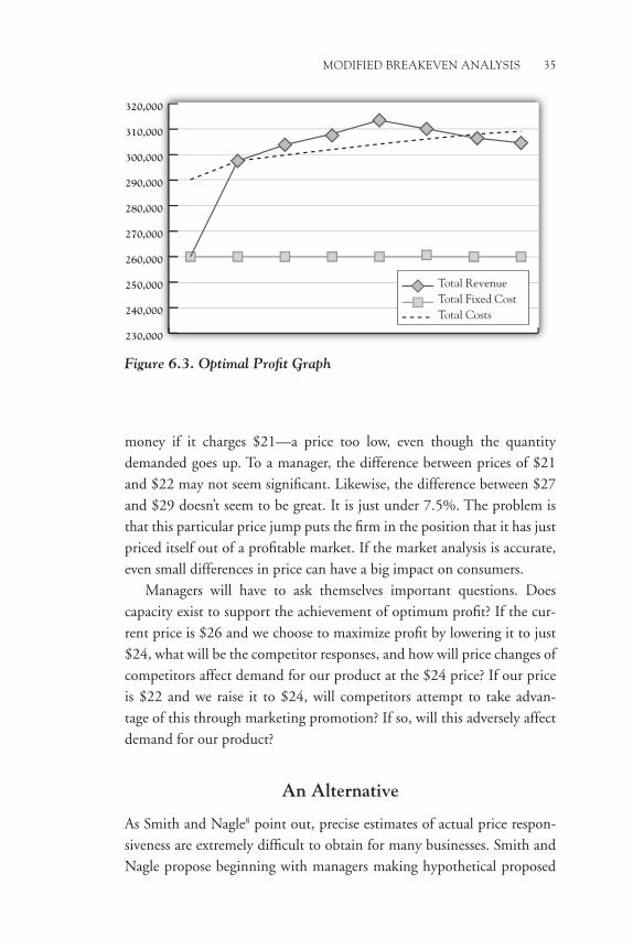
MoDiFiED BrEakEvEn analysis 35
money if it charges $21—a price too low, even though the quantity demanded goes up. To a manager, the difference between prices of $21 and $22 may not seem significant. Likewise, the difference between $27 and $29 doesn’t seem to be great. It is just under 7.5%. The problem is that this particular price jump puts the firm in the position that it has just priced itself out of a profitable market. If the market analysis is accurate, even small differences in price can have a big impact on consumers.
Managers will have to ask themselves important questions. Does capacity exist to support the achievement of optimum profit? If the cur-rent price is $26 and we choose to maximize profit by lowering it to just $24, what will be the competitor responses, and how will price changes of competitors affect demand for our product at the $24 price? If our price is $22 and we raise it to $24, will competitors attempt to take advan-tage of this through marketing promotion? If so, will this adversely affect demand for our product?
an alternative
As Smith and Nagle8 point out, precise estimates of actual price respon-siveness are extremely difficult to obtain for many businesses. Smith and Nagle propose beginning with managers making hypothetical proposed
230,000
240,000
250,000
260,000
270,000
280,000
290,000
300,000
310,000
320,000
Total RevenueTotal Fixed CostTotal Costs
Figure 6.3. Optimal Profit Graph

36 BrEakEvEn analysis
price changes, calculating the breakeven point for each, and then estimat-ing the degree of responsiveness (price elasticity of demand) customers are likely to have to such price proposals.
The first step is to calculate the breakeven point for a product (using the traditional breakeven analysis formula) at different levels of price. For example, Table 6.2, Breakeven Points at Different Price Levels, might be constructed for a corporation.
The selling price (SP) of $80 was chosen in this illustration. Using information from the table, a graph can be drawn showing the breakeven points at different levels of price. Construct the graph, plotting the price on the vertical axis and the unit sales volume on the horizontal axis. The line drawn through each of the breakeven points on the graph becomes the “constant profit” curve, or the line on which breakeven is achieved at each price level. See Figure 6.4, Constant Profit Curve at Various Prices.
In Figure 6.4, the price of $80 is the current price. At this price the breakeven sales volume is 50,000 units. To the constant profit curve can be added hypothetical demand curves illustrating the degree of responsiveness to price. One demand curve (labeled “A” in Figure 6.5, Inelastic Demand Curve) shows that customers are less responsive to price changes (relatively inelastic demand). To the right of the demand curve, losses will occur if prices are changed in this direction (reduced). To the left of the demand curve, gains will occur if prices are changed in this direction (increased).
Table 6.2. Breakeven Points at Different Price Levels
% D in Sp Sp ($) CM2 ($) BeU
% Change Be Sales
Change in Units
25.0% 100 40 25,000 –50.0% –25,000
20.0% 96 36 27,778 –44.4% –22,222
15.0% 92 32 31,250 –37.5% –18,750
10.0% 88 28 35,714 –28.6% –14,286
5.0% 84 24 41,667 –16.7% –8,333
0.0% 80 20 50,000 0.0% 0
–5.0% 76 16 62,500 25.0% 12,500
–10.0% 72 12 83,333 66.7% 33,333
–15.0% 68 8 125,000 150.0% 5,000
–20.0% 64 4 250,000 400.0% 200,000

MoDiFiED BrEakEvEn analysis 37
Notice that the demand curve “A” crosses the constant profit curve when price equals $80 (the current price). If the price is changed, the cur-rent price becomes the “baseline” against which customer responsiveness must be evaluated.
Figure 6.4. Constant Profit Curve at Various Prices
Figure 6.5. Inelastic Demand Curve

38 BrEakEvEn analysis
Figure 6.6. Elastic Demand Curve
The other hypothetical demand curve shown below indicates more responsiveness to price changes. The demand curve “B” in Figure 6.6, Elas-tic Demand Curve, is flatter than demand curve “A” in Figure 6.5. The flat-ter demand curve illustrates that when prices are increased above $80, losses will likely occur since customers are more responsive to price increases. But when prices are reduced below $80, more customers will buy the product, and as a result gains will be achieved.
The benefit of using this type of graph over attempting to calculate the precise demand is that the manager simply has to make an informed judg-ment as to whether customer responsiveness is likely to be greater or less than the level required to achieve breakeven.
Table 6.2 and Figures 6.4 through 6.6 put forward by Smith and Nagle still require managers to make an informed judgment regarding the price elasticity of demand (customer responsiveness to changes in price)—the slope of the demand curve. The marginal advantage their approach provides during managerial discussions is that the table and graphs will encourage dialog and debate over the assumptions regarding customer responsiveness at various hypothetical prices.

MoDiFiED BrEakEvEn analysis 39
the ethical Dimension
If customers continue to buy a product even though the price goes up, everything else being equal, total revenue and total profit will increase. Such an action may provide a short-run economic payoff. In the long run, any of several things will probably happen. First, some customers will find out about this and turn against the company, creating demand for a substitute. Second, even though the availability of substitutes is low, other customers will just not purchase, choosing to go without and wait for a substitute. Third, this action will entice competitors into the market. In any case, if customers choose to sit out or if more competitors enter the market, mar-ket prices and industry profits will tend to go down. Thus company man-agers who try to capture too much short-run profit may very likely find that they have unintentionally brought about the demise of the very thing they hoped to achieve.
Considering customer responsiveness has an important ethical dimen-sion. For example, if company managers determine that customers are relatively unresponsive to changes in price because few readily available substitutes are present in the market, is it moral for those managers to take advantage of the situation in order to capture more revenue by raising the price even if their costs remain unchanged? It can be argued that to use the degree of customer responsiveness against customers by raising prices above what would be reasonably expected is unethical.
We have already introduced the idea that many companies sell more than just one product. We turn next to consider another approach to han-dling this type of situation.


Chapter 7
Dealing With Changes in product Mix Using
Weighted averages
As we have seen, product mix is one of the most important influences on breakeven point. Change the product mix, and if there are wide dif-ferences in variable costs and selling prices in the mix, the profitability can change quickly.
In this chapter we will focus on two breakeven methods that employ weighted averages. The first is the weighted average contribution margin method, and the second is the weighted average selling prices method.
the Formula
The product mix can be used to determine the weighted average contri-bution margin as is shown in the following formula:
Breakeven Units (BEU) = Fixed Costs ÷ Weighted Average
Contribution Margin.
Breakeven and cost-volume-profit analysis are typically explained and illustrated with single-product or single-service organizations. In reality, most organizations offer more than one product or service. We refer to these multiple products or services as the sales mix. We need a method to apply cost-volume-profit analysis to commercial reality.
An appliance store, for example, might track sales of various brands and types of appliance (refrigerators, ranges, dishwashers, etc.). It might also track repair service on appliance brands, warranty and out-of-warranty service, and service on different types of appliances. Each of

42 Breakevenanalysis
these sources of revenue could produce a different contribution margin (CM). Let’s look at an example.
example 1
Bob’s Appliances has provided us with the data in Table 7.1, Sales Mix.After calculating the weighted average contribution margin, the
breakeven calculation is the same:
$448,400 Bob’s
Annual Fixed Costs=
1,900 Total Units to
Be Sold Annually.$236 Weighted
Average CM
However, the 1,900 units to be sold to break even must be sold in the proportions stated in the sales mix: 950 refrigerators (1,900 × 50%), 380 dishwashers (1,900 × 20%), and 570 repair service calls (1,900 × 30%).1
Using Table 7.2, Sales Mix Quantities to Be Sold, we can check to be sure these sales quantities will bring Bob to break even. If Bob adds a desired profit, the calculation is
$448,400 Annual Fixed Costs
+ $17,700 Desired Profit=
1,975 Units to Be
Sold Annually.$236 Weighted Average CM
One of our limiting assumptions of cost-volume-profit analysis is that the sales mix must remain constant for the results to be meaningful. Let’s exam-ine what happens to Bob’s Appliances if his sales mix changes (Table 7.3, Changing Sales Mix). Bob sold the overall total units required, 1,900, but because he sold more low contribution margin units and fewer high contri-bution margin units (the sales mix changed), he failed to achieve breakeven.
Table 7.1. Sales Mix
Sales mix CM per unit Weighted CMrefrigerators 50% $350 $175=($350×50%)
Dishwashers 20% $200 $40=($200×20%)
repairservicecalls 30% $70 $21=($70×30%)
WeightedaverageCM $236

DealingWithChangesinProDuCtMix 43
Benefits
For some companies circumstances may make it difficult for manag-ers to identify unit variable costs. A company that sells dozens or even scores of different products might employ a spreadsheet or other com-puter software to make the calculations less tedious. Once the spread-sheet is set up, sensitivity analysis can be used to monitor the impact on breakeven if demand changes for certain products or packages of products.
As with other methods, thinking about breakeven naturally should lead directly to thinking about operations. The more products a company pro-duces, the more managers will be interested in finding synergies between these products so that production is achieved by sharing critical resources across more than one product. Such synergies have the potential of lowering costs, making the breakeven point easier to achieve.
Table 7.2. Sales Mix Quantities to Be Sold
Units sold CM per unit total CM earnedrefrigerators 950 $350 $332,500($350×950)
Dishwashers 380 $200 $76,000($200×380)
repairservicecalls 570 $70 $39,900($70×570)
totalunitssold 1,900
totalCMearned $448,400
Fixedcosts $448,400
netincomeorloss $0
Table 7.3. Changing Sales Mix
Units sold CM per unit total CM earnedrefrigerators 850 $350 $297,500($350×850)
Dishwashers 480 $200 $96,000($200×480)
repairservicecalls 570 $70 $39,900($70×570)
totalunitssold 1,900(asindicatedbythebreakeven
calculation)
totalCMearned $433,400
Fixedcosts $448,400
netloss ($15,000)

44 Breakevenanalysis
In some situations or companies, managers choose not to go through the time and expense of identifying unit variable costs. These managers might benefit from the next method highlighted in this chapter: weighted average selling price.
Weighted average Selling price Method
For organizations that sell essentially one service but at different prices, breakeven can be calculated even if the unit variable costs are not known. Because of the differences in prices, the product mix still heavily influences the breakeven point. For example, a minor league baseball club sells essen-tially the same entertainment “product” to all who attend its home games but at three different prices for children, adults, and senior citizens. Differential pricing is usually charged for seat location in the ballpark. The Grand Ole Opry sells tickets to the same event but at different prices depending on loca-tion of seating. A hotel rents rooms but at different prices depending on the season of the year or the distribution channels used in marketing. Airlines sell seats on flights at different prices depending on season, timing of pur-chase, and the marketing organization used to sell tickets. Such managers may choose this approach to focus on the marketing side of the business.
Like total sales revenue, the unit selling price is often known when other details are not as readily known. Total costs may be known when variable costs cannot be distinguished from fixed costs. Under these conditions the weighted average selling price method can be useful.
the Formula
The weighted average selling price method allows for the calculation of breakeven using the following formula:
BEU = Total Costs ÷ Weighted Average Selling Price.
Notice in this method that we are comparing company total costs as a whole group and selling price of the company’s products as a weighted group. Total costs, for most companies, requires a straightforward pro-cess of simply summing all costs for a relevant period of time. Unlike other breakeven formulas, no distinction is made between fixed costs and variable costs.

DealingWithChangesinProDuCtMix 45
Weighting the selling price is accomplished by taking each product and multiplying its selling price by the proportion of the total units sold. This is the weighted selling price for one product. The sum of the weighted selling prices for all products is the weighted average selling price for the company’s products as a group.
Note that calculating a weighted average is not the same as calculating the simple average. For example, see Table 7.4, Comparison of Simple and Weighted Average Selling Price, listing four products and the selling price (SP) for each.
Simple average (also known as the mean) selling price (SP) is calcu-lated by adding the four selling prices and dividing by the number of different products (in this case, there are four) offered in the market. In Table 7.4 the simple average is $59.95. Weighted average selling price is $4 less than the simple average selling price. In this case, using the simple average price would underestimate the breakeven point. In another case, the weighted average selling price might be more than the simple average, in which case the breakeven point would be overestimated if the simple average were used.
Now let’s use this in a couple of examples.
example 2
For 20 years Olympia Community Theater has been selling tickets to its annual 3-week production of Fiddler on the Roof. The Board of Trust-ees for Olympia has decided that this year Olympia should sell tick-ets at three different prices: $6 (children), $10 (adults), and $8 (senior citizens). For the production, Olympia Community Theater Company rents the old and quite small (125 seats) Paramount Theater. It also rents
Table 7.4. Comparison of Simple and Weighted Average Selling Price
products Sp Sales mix Weighted average Sproyal $29.95 35.0% $10.48
excelsior $49.95 25.0% $12.49
galaxy $69.95 15.0% $10.49
ultra $89.95 25.0% $22.49
total 100.0% $55.95
simpleaverage $59.95

46 Breakevenanalysis
props, lighting equipment, and costumes, using these resources for a total of 15 performances of the play. Several thousand dollars are spent on promotional materials including the printing of the program, tickets, and posters. Olympia also pays an honorarium to local musicians who partici-pate in the pit orchestra. Total costs for the production equal $12,650. The question the producer wants answered is, how many tickets must we sell to break even?
The weighted average selling price is shown in Table 7.5, Weighted Average Ticket Price. Sales mix is based on historical trends over the last two decades.
With this information, the breakeven point is calculated as follows:
CT = Total Costs
SPWT = Weighted Average Selling Price
BEU = CT ÷ SPWT = Number of Tickets Sold to Break Even
BEU = $12,650 ÷ $8.80
BEU = 1,438 Tickets Sold.
Over a 3-week period with five shows produced each week, the average attendance needs to be represented by 96 tickets sold for each show. This is 77% of capacity. Using the historical trend data on sales mix, we can see that to break even on its production of Fiddler on the Roof, Olympia will sell 288 tickets for children, 863 adult tickets, and 288 tickets to senior citizens.
example 3
Consider Peninsula Consulting, a professional financial service organiza-tion that offers four levels of service to privately owned businesses each at a different price: $2,295 (Basic), $2,995 (Advanced), $3,495 (Silver), and
Table 7.5. Weighted Average Ticket Price
Children adults Seniors totalsalesmix 20% 60% 20% 100%
sP $6 $10 $8
Wtd.averagesP $1.20 $6 $1.60 $8.80

DealingWithChangesinProDuCtMix 47
$3,995 (Platinum). Small businesses “subscribe” annually to receive advice on finance issues throughout the year, assistance with year-end taxes, and production of year-end financial statements. To deliver the promised ser-vices, Peninsula Consulting incurs total costs of $950,000 annually. The sales mix is shown in Table 7.6, Peninsula Consulting Sales Mix.
The weighted average selling price is $2,965 per service package. To break even, Peninsula Consulting must sell a total of 320 service packages at the given sales mix.
Interpreting the result
Similar to the contribution margin method considered elsewhere in this book, the weighted average selling price method casts the result in terms of units of product or service sold. Because of this, breakeven analysis should lead managers naturally to think about the operational issues such as capacity, staffing, marketing, and organization. In the previous exam-ple, if Peninsula Consulting learns that it is easier to sell Basic Service packages and very difficult to sell Platinum Service packages, the sales mix and the breakeven point will most likely change.
As the top managers of Peninsula staff and organize the company, they must ask what staffing mix is required to provide Basic Service to 120 clients, Advanced Service to 80 clients, Silver Service to 64 clients, and Platinum Service to 48 clients. For example, the number of account-ing professionals and their support staff needed to provide Platinum Ser-vice for every 10 clients may be quite different from that required to provide Basic Service.
Anytime sales mix (also known as product mix) is factored into breakeven analysis, the need for accurate and timely data becomes vital. Managers who use this method must closely track sales mix. As actual
Table 7.6. Peninsula Consulting Sales Mix
Basic Service
advanced Service
Silver Service
platinum Service
total
salesmix 40% 25% 20% 15% 100%
sP $2,295 $2,995 $3,495 $3,995
Wtd.averagesP $918 $749 $699 $599 $2,965
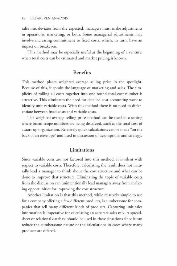
48 Breakevenanalysis
sales mix deviates from the expected, managers must make adjustments in operations, marketing, or both. Some managerial adjustments may involve increasing commitment to fixed costs, which, in turn, have an impact on breakeven.
This method may be especially useful at the beginning of a venture, when total costs can be estimated and market pricing is known.
Benefits
This method places weighted average selling price in the spotlight. Because of this, it speaks the language of marketing and sales. The sim-plicity of rolling all costs together into one round total-cost number is attractive. This eliminates the need for detailed cost-accounting work to identify unit variable costs. With this method there is no need to differ-entiate between fixed costs and variable costs.
The weighted average selling price method can be used in a setting where broad-scope numbers are being discussed, such as the total cost of a start-up organization. Relatively quick calculations can be made “on the back of an envelope” and used in discussion of assumptions and strategy.
Limitations
Since variable costs are not factored into this method, it is silent with respect to variable costs. Therefore, calculating the result does not natu-rally lead a manager to think about the cost structure and what can be done to improve that structure. Eliminating the topic of variable costs from the discussion can unintentionally lead managers away from analyz-ing opportunities for improving the cost structure.
Another limitation is that this method, while relatively simple to use for a company offering a few different products, is cumbersome for com-panies that sell many different kinds of products. Capturing unit sales information is imperative for calculating an accurate sales mix. A spread-sheet or relational database should be used in these situations since it can reduce the cumbersome nature of the calculations in cases where many products are offered.

DealingWithChangesinProDuCtMix 49
When this method is used to help project the expected future experi-ence of an organization, the whole exercise will turn on the accuracy of the assumptions regarding total costs and the assumptions about market prices and sales mix. Inaccuracies in these assumptions will drive spurious breakeven analysis results.

Chapter 8
high-Low Method
For costs that are neither purely variable nor purely fixed, we must iden-tify and separate those variable and fixed components to be able to incor-porate them into our cost-volume-profit analysis. The high-low method is a simple way to accomplish that objective.
We will continue with the example of Bob’s Appliances. Bob delivers the new appliances he sells to customers. Some of the costs associated with this delivery service are fixed, such as insurance, emissions inspec-tions for his trucks, and depreciation. Other costs, such as gasoline and tires, are variable, based on the number of deliveries he makes and the miles he travels per year. In the most current year, Bob made 180 deliver-ies and incurred a total delivery cost of $2,800. These will be our “high” values. In the immediately preceding year, Bob made 140 deliveries and incurred an annual delivery cost of $2,500. These will be our “low” val-ues. Begin the analysis by expressing the data this way:1
$2,800 Current Year Costs – $2,500 Preceding Year Costs = $300
Change in Costs
180 Current Year Deliveries – 140 Preceding Year Deliveries = 40
Change in Deliveries
Variable Cost per Delivery = $300 ÷ 40 = $7.50
To find the fixed cost component, use the “high” values: 180 deliveries and $2,800 costs.
Total Costs = $2,800
Total Variable Costs = (180 Deliveries × $7.50 Variable Cost
per Delivery) = $1,350
Total Fixed Costs per Year = $2,800 – $1,350 = $1,450

52 Breakevenanalysis
Some people find that organizing the data into a matrix is useful in mak-ing the calculation as illustrated in Table 8.1, High-Low Example. Use the same method as shown previously to find the fixed cost amount.
You may be presented with daily, weekly, monthly, or other periodic data. You may have a large amount of data to work with. However, the high-low method always uses only the highest unit or activity value and the lowest unit or activity value. All other data are disregarded. This fea-ture of the high-low method makes it subject to misinformation if the high or low values are anomalies (statistically referred to as outliers). If the high cost value is unusually large or the low cost value is unusually small, the variable cost per unit will be overstated and the total fixed cost will be understated. Table 8.2, Outlier Example, is an illustration of the effect of an outlier.
The variable cost per unit, in the outlier example, is overstated by $5 per unit. What about the fixed cost per year?
Total Costs = $3,000 (Outlier Cost Amount)
Less Total Variable Costs = $2,250 (180 Deliveries × $12.50 Variable
Cost per Delivery)
Equals Total Fixed Costs = $750 per Year
Table 8.1. High-Low Example
Cost UnitsHighvalue $2,800 180
lowvalue $2,500 140
Difference $300 40
Calculation $300÷40=$7.50variableCostperDelivery
Table 8.2. Outlier Example
Cost UnitsHighvalue* $3,000 180
lowvalue $2,500 140
Difference $500 40
Calculation $500÷40=$12.50variableCostperDelivery
*This cost amount is unusually high, an outlier.

HigH-lowMetHoD 53
Comparing the $1,450 annual fixed cost using normal values from our first example with the $750 annual fixed cost using an outlier value, the annual fixed cost, using the outlier value, is understated by almost half.
Another potential for misinterpretation is illustrated by Table 8.3, Maintenance Costs Versus Miles Driven.
The proper choice for the high value is the highest number of miles driven (the highest activity level). However, when placed in the formula, the data mathematically produce a negative value for variable cost per mile driven. The result is clearly unreasonable. You will need to choose a different time period for analysis or try grouping the months into quar-ters or years to avoid these nonsense results.
One of the limiting assumptions is that there is no inflation or defla-tion to distort the results. Inflation or deflation tends to cause fixed costs to appear to be variable costs. When evaluating costs that have fixed quantities associated with them (such as utilities or fuel consumed, lum-ber used, labor hours worked), the quantity of the item consumed may be used instead of the dollar cost to calculate the variable and fixed amounts. Then, a dollar amount is applied.
Statewide Industries uses large quantities of natural gas to produce its product. In the current year, it used 1,000,000 mcf (million cubic feet) to produce 800,000 units of finished product. In the immediately preced-ing year, the company used 920,000 mcf to produce 740,000 units of finished product. See Table 8.4 Natural Gas Use.
Table 8.3. Maintenance Costs Versus Miles Driven
Maintenance cost Miles drivenJanuary $1,000 11,200
February $900 10,600
March $800 11,300
Table 8.4. Natural Gas Use
mcf UnitsHighvalue 1,000,000 800,000
lowvalue 920,000 700,000
Difference 80,000 100,000
Calculation 80,000÷100,000=0.80mcfvariableUsage(Cost)perUnit

54 Breakevenanalysis
Table 8.5, Fixed Cost Calculation, illustrates the calculation of fixed usage.
After obtaining the variable and fixed rates, you may apply the appro-priate cost per mcf. If the utility company is charging $2.40 per mcf, then your variable cost per unit would be (.8 mcf × $2.40) = $1.92. The fixed cost would be (360,000 mcf × $2.40) = $864,000.
One of the things we are trying to achieve with the high-low method is a separation of total (mixed) costs into a fixed cost component and a variable cost component. An alternative way of thinking about the rela-tionship between the high and the low is this formula:
Total Mixed Costs = Fixed Cost Component + (Slope × Variable Cost
Component).
Putting in the familiar algebra format, we get
Y = a + bX,
where
Y = Total Mixed Costs
a = Fixed Cost Component
b = Unit Variable Cost Component (Slope of the Line)
X = Number of Units Produced and Sold.
This formula depicts the relative differences in cost and volume as a lin-ear relationship between the highest point and the lowest point in terms of values of cost and their corresponding activity levels. We can think of this method as employing the highest point of costs and the lowest point of costs with a sloped line that connects these two points.
Table 8.5. Fixed Cost Calculationtotalusage 1,000,000 mcf
lesstotalvariableusage
640,000 (800,000Units×0.80mcfvariableusageperunit)
equalstotalfixedusage 360,000 mcf
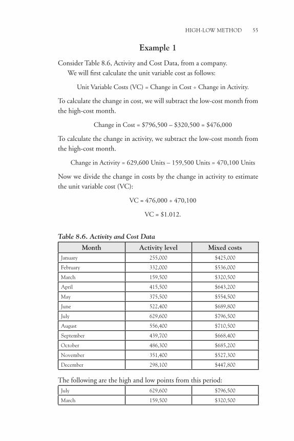
HigH-lowMetHoD 55
example 1
Consider Table 8.6, Activity and Cost Data, from a company.We will first calculate the unit variable cost as follows:
Unit Variable Costs (VC) = Change in Cost ÷ Change in Activity.
To calculate the change in cost, we will subtract the low-cost month from the high-cost month.
Change in Cost = $796,500 – $320,500 = $476,000
To calculate the change in activity, we subtract the low-cost month from the high-cost month.
Change in Activity = 629,600 Units – 159,500 Units = 470,100 Units
Now we divide the change in costs by the change in activity to estimate the unit variable cost (VC):
VC = 476,000 ÷ 470,100
VC = $1.012.
Table 8.6. Activity and Cost Data
Month activity level Mixed costsJanuary 255,000 $425,000
February 332,000 $536,000
March 159,500 $320,500
april 415,500 $643,200
May 375,500 $554,500
June 522,400 $689,800
July 629,600 $796,500
august 556,400 $710,500
september 439,700 $668,400
october 486,300 $685,200
november 351,400 $527,300
December 298,100 $447,800
The following are the high and low points from this period:
July 629,600 $796,500
March 159,500 $320,500
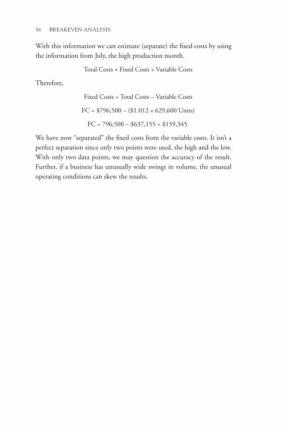
56 Breakevenanalysis
With this information we can estimate (separate) the fixed costs by using the information from July, the high production month.
Total Costs = Fixed Costs + Variable Costs
Therefore,
Fixed Costs = Total Costs – Variable Costs
FC = $796,500 – ($1.012 × 629,600 Units)
FC = 796,500 – $637,155 = $159,345.
We have now “separated” the fixed costs from the variable costs. It isn’t a perfect separation since only two points were used, the high and the low. With only two data points, we may question the accuracy of the result. Further, if a business has unusually wide swings in volume, the unusual operating conditions can skew the results.

Chapter 9
Least Squares Method
As explained in the previous chapter, when costs are neither purely vari-able nor purely fixed, we must identify and separate those variable and fixed components to be able to incorporate them into our cost-volume-profit analysis. The least squares method is a more precise mathematical approach to accomplish that objective. Let’s expand on the example of Bob’s Appliances. Over the past several years, Bob’s volume of deliveries and delivery costs has varied from year to year as shown in Table 9.1, Deliveries and Costs.
Notice that the last 2 years contain the same data we used in the high-low method to determine the variable delivery cost per unit ($7.50) and the fixed delivery cost per year ($1,450).
To find the variable and fixed cost components of the delivery cost, follow these steps.1
Step 1: Enter your unit and cost data in a spreadsheet, as shown in Figure 9.1 (see columns B and C).
Step 2: To find the variable cost per delivery, enter the formula =linest(C4:C8,B4:B8). In Figure 9.1 this formula has been entered into cell B10.
In Figure 9.1, Calculating Variable Delivery Cost, the example spreadsheet gives the variable cost per delivery as $7.85.
Table 9.1. Deliveries and Costs
Year Units delivered Delivery costs20AA 160 $2,700
20AB 170 $2,795
20AC 150 $2,610
20AD 140 $2,500
20AE 180 $2,800

58 BrEAkEvEnAnAlysis
Step 3: To find the fixed delivery cost per year, enter the formula =intercept(C4:C8,B4:B8). In the Figure 9.2, Calculating Fixed Delivery Costs, this formula has been entered into cell B11. The example spreadsheet gives the fixed delivery cost as $1,425 per year.
Figure 9.1. Calculating Variable Delivery Cost
Figure 9.2. Calculating Fixed Delivery Costs

lEAstsquArEsMEthoD 59
Essentially, the spreadsheet is taking all the data (not just the highest and low-est values) and helping us find the fixed cost component (intercept) and the variable cost component (linest) from the following formula that we intro-duced in the last chapter:
Y = a + bX,
where
Y = Total (mixed) Costs of Delivery
a = Fixed Cost Component
b = Unit Variable Cost Component (Slope of the Line)
X = Number of Units Produced and Delivered.
This approach produces a mathematical estimate. But how precise is our estimate? To determine this we calculate a coefficient of determination.
Step 4: To find the coefficient of determination (often written R2), enter the formula =RSQ(C4:C8,B4:B8). This formula has been entered into cell B12, shown in Figure 9.3, Calculating the Coefficient of Determination.
Figure 9.3. Calculating the Coefficient of Determination

60 BrEAkEvEnAnAlysis
The example spreadsheet gives the coefficient of determination as 0.94. You may interpret the coefficient of determination as telling you that the changes in the volume of units delivered explain 94% of the changes in delivery costs incurred. Other changes in the business model not factored into this mathe-matical model explain only 6% of the changes in delivery costs. We conclude in this case that the values calculated for the variable and fixed cost components of delivery cost for Bob’s Appliances are very good estimates of Bob’s costs. Every company is different in terms of the changes that occur in the volume of units produced and sold and how these changes affect changes in costs.
Compare the results of the least squares method with the results of the high-low method discussed in the preceding chapter. This is shown in Table 9.2, Comparison of High-Low and Least Squares Results.
At the low volumes illustrated by Bob’s Appliances, the difference between the two methods might be immaterial. However, at high volumes, the differ-ence between the two methods could be substantial. The least squares method will produce the better estimates.
Why are the calculated values referred to as estimates when the spread-sheet process looks very precise? Let’s select the most recent year, 20AE, and test the least squares values we calculated.
Total Variable Cost = $1,413 (180 Units × $7.85 per Unit)
Total Fixed Cost = $1,425
Total Costs = $2,838 Based on Least Squares
Cost Estimates
We observe from the data that actual costs in year 20AE were $2,800, while the total costs calculated from our estimates are slightly different. This dif-ference is a normal aspect of the mathematical process inherent in the least squares method.
You may be presented with daily, weekly, monthly, or quarterly data. You may have a large amount of data to work with. Unlike the high-low method of the preceding chapter, the least squares method considers all data available in
Table 9.2. Comparison of High-Low and Least Squares Results
Method Variable costs Fixed costshigh-lowmethod $7.50perdelivery $1,450peryear
leastsquaresmethod $7.85perdelivery $1,425peryear

lEAstsquArEsMEthoD 61
calculating the cost estimates. As with the high-low method, outliers (abnormal values) can distort the results.
As explained previously, one of the limiting assumptions is that there is no inflation or deflation to distort the results. Inflation or deflation tends to cause fixed costs to appear to be variable costs. The process of excluding the effect of inflation or deflation would be the same as for the high-low method.
Multiple regression, a more complex application of the least squares method, considers the effect on costs of several variables. Substantial business judgment and caution should be exercised in the selection of the variables. The multiple regression calculations can be performed with ease using statis-tics software such as SPSS. Application of multiple regression is beyond the scope of this book.
Using the Scattergraph
The scattergraph is a visual way to understand the coefficient of determina-tion. Each data point is plotted on a graph. Then a line (called a trend line) is drawn to minimize the distances from the data points to the line. We do this to determine the “goodness of fit.” Notice that all the data points are very near the trend line (a very good fit), which indicates a close relationship between changes in the number of units delivered and changes in the delivery costs.2 An example of a scattergraph depicting a very good fit is shown in Figure 9.4, Scattergraph A.
In contrast, consider this next scattergraph shown in Figure 9.5, Scatter-graph B. Notice that some of the data points do not lie very near the trend line. In fact, the point for 200 units delivered is quite far from the trend line. This off-the-line data point is called an outlier. There is an unusual cost-volume relationship in the year 20AH.3 Also, contrast the first graph’s R2 value of 0.94, indicating a very close linear cost-volume relationship, with the second graph’s R2 value of only 0.74, indicating a less linear cost-volume relationship. This lower value of 0.74 would indicate that the variable and fixed cost estimates calculated are very rough (imprecise) estimates.
Finally, notice in Figure 9.6, Scattergraph C, how all remaining data points lie very near the trend line when the outlier is removed.4 The R2 value rises dramatically to 0.99, with no outlier data. The variable and fixed cost esti-mates calculated here are very good representatives of Bob’s actual cost behavior.

62 BrEAkEvEnAnAlysis
Figure 9.4. Scattergraph A
Figure 9.5. Scattergraph B

lEAstsquArEsMEthoD 63
Figure 9.6. Scattergraph C


Chapter 10
Changing Costs
Our friend Bob, with whom we are getting quite well acquainted by now, is experiencing rising costs for the appliances he sells. He is wondering how this change will affect his breakeven point. Table 10.1, Refrigerator Contribution Margin, represents a typical refrigerator sale for Bob.
Here is Bob’s breakeven point before the change in cost:
$437,500 Annual Fixed Costs=
1,250 Total Units to
Be Sold Annually.$350 CM
This translates into $1,250,000 sales ($1,000 per unit × 1,250 refrigera-tors) needed to break even.
Recently, the manufacturer notified Bob that his cost to purchase a refrigerator would go up from $650 to $700. Assume that local competi-tion will not allow Bob to increase the selling price of his refrigerators. Now, the typical refrigerator sale looks like the information portrayed in Table 10.2, Contribution Margin With Cost Inflation.
Here is Bob’s breakeven point after the change in cost:
$437,500 Annual Fixed Costs=
1,459 Total Units to
Be Sold Annually.$300 CM
Table 10.1. Refrigerator Contribution MarginSelling price to the customer $1,000 100%
Bob’s purchase cost $650 65%
Bob’s contribution margin (CM) $350 35% contribution margin ratio
Table 10.2. Contribution Margin With Cost InflationSelling price to the customer $1,000 100%
Bob’s purchase cost $700 70%
Bob’s contribution margin $300 30% contribution margin ratio

66 Breakeven analySiS
This translates into $1,459,000 sales ($1,000 × 1,459 refrigerators) needed to break even.
Now, let’s change the scenario. Assume local competition will allow Bob to increase the selling price of refrigerators to reflect his increased cost. Bob may want to keep the contribution margin amount per refrig-erator constant. In that event, his new breakeven calculation is shown in Table 10.3, Contribution Margin With New Selling Price.
Here is Bob’s breakeven point after the changes in cost and selling price:
$437,500 Annual Fixed Costs=
1,250 Total Units to Be
Sold Annually.$350 CM
Amazingly, Bob’s breakeven point in units to be sold is unchanged from his original numbers, before the cost increased. However, he must sell $1,312,500 (instead of $1,250,000) to break even.
Bob might, instead, want to earn the same contribution margin ratio on his sales. His new breakeven calculation can be obtained from the data shown in Table 10.4, Target Contribution Margin Ratio.
Here is Bob’s breakeven point after the change in cost:
$437,500 Annual Fixed Costs=
1,161 Total Units to
Be Sold Annually.$377 CM
Remarkably, Bob can break even by selling fewer refrigerators after the cost increase when he holds his contribution margin ratio unchanged.
Table 10.3. Contribution Margin With New Selling PriceSelling price to the customer $1,050 100%
Bob’s purchase cost $700 66.67%
Bob’s contribution margin $350 33.33% contribution margin ratio
Table 10.4. Target Contribution Margin RatioSelling price to the customer $1,077 100% ($700 ÷ 0.65)
Bob’s purchase cost $700 65%
Bob’s contribution margin $377 35% target contribution margin ratio

Changing CoStS 67
Changing the Variable Costs of Manufacturing
A retailer like Bob has one way to deal with the decision of what to do as costs change. Changing variable costs creates a similar challenge for manufacturing firms whose managers need to know the impact of such changes on the breakeven point. Sometimes without warning suppliers will take an action that has an immediate, direct effect on the unit vari-able cost. While they can lower their prices, it is the increase in costs of input factors that will be the dominant concern when considering the impact of such changes on the breakeven point.
The application of breakeven analysis reviewed here seeks to answer a simple question: “How would a change in variable cost affect the sales goals to generate equal or better profit?” This application of breakeven analysis takes as a given that the current level of profit is acceptable to managers. Fixed costs and selling price are assumed to remain unchanged.
The application is built on the change in contribution margin that a change in variable costs represents.
More specifically, a formula provided by Smith and Nagle1 is helpful:
% Change in Sales Volume Needed = –Change in Contribution Margin
÷ (Contribution Margin + Change in Contribution Margin).
Using algebra notation we can simplify this with the following:
%D Sales = –DCM ÷ (CM + DCM),
where
%D Sales = % Change in Sales Units Needed to Generate Equal Profit
DCM = Change in Contribution Margin (Measured in Dollars)
CM = Contribution Margin (in Dollars).
Assuming that fixed costs or selling price does not change as a result of the change in variable costs, this formula calculates the minimum per-cent change in sales volume at the new variable cost needed to generate the same level of profit. But variable costs can go up or down. When variable costs go down, generally this relieves some of the pressure to achieve the sales volume required to achieve desired profit. When vari-able costs go up, it puts additional pressure on sales volume to achieve

68 Breakeven analySiS
desired profit. It is an increase in variable costs that we will most often be concerned about.
Increases in variable costs can come from many places, such as new marketing ideas like product packaging, product design changes, or prod-uct style changes. Another source of change is when suppliers of compo-nents and materials raise their prices.
To see how this simple formula works, consider the following example.
Heartland Machine, Inc.
Heartland Machine, Inc., sells 10,000 specially designed machine tools annually for total global sales revenue of $14,000,000. That’s $1,400 per unit selling price. The marketing manager proposed using new, more expensive packaging that would cost $45 per unit. In effect, this change would raise the unit variable cost by 4.09%. He argued that better pack-aging would give distributors an advantage in selling the machine tools to their customers. Packaging is an important signal to customers of the value they are getting. The logic was that if distributors promoted the product more because of the exciting packaging, Heartland would sell more machine tools and generate more revenue and more profit.
The general manager was not immediately convinced. He said, “Fine. But before we implement new product packaging, I need to know the impact on sales that we need to see in order to maintain or improve upon current profit.”
Unit Variable Costs for the Heartland Machine tool equal $1,010 per unit. Subtracting the unit variable cost from the unit selling price of $1,400 reveals the unit contribution margin of $390. This assumes that the selling price will remain unchanged.
The minimum percent increase in sales volume needed to maintain the same level of profit after the increase to variable costs is as follows:
%D Sales Units = –DCM ÷ (CM + DCM)
= –(–45) ÷ (390 – 45)
= 45 ÷ (345)
= 13.04%

Changing CoStS 69
In this case a 13% increase in sales volume is needed to maintain the same level of profit after the addition of new packaging. The sales man-ager might have an opinion regarding the likelihood of achieving this.
The results of this shorthand method can be confirmed using the tra-ditional breakeven analysis formula as shown in Table 10.5, Changing Variable Costs at Heartland Machine, where breakeven point in units (BE
U) equals fixed costs (FC) divided by the contribution margin (CM),
or BEU = FC ÷ CM.
Impact of Changing Fixed Costs
Adding fixed costs to an organization is sometimes necessary for the orga-nization to continue carrying out its mission. A manager may need to be added. Extra employees may be needed in the assembly line or packing and shipping department. Customer service may need more trained staff. Sales personnel may need to be hired and trained. Additional money may need to be spent on advertising to stimulate demand. What is common to all these additions to fixed cost is that the contribution margin must “carry” a heavier weight than before. This means that the volume of sales needed to break even increases.
Calculating the impact from a change in fixed costs on profit is straightforward using the following formula: % Change in Sales Units Needed = % Change in Fixed Costs:
%D Sales = %D FC,
Table 10.5. Changing Variable Costs at Heartland Machine
Before after Change % Change
Fixed costs $3,900,000 $3,900,000 0 0.00%
variable costs $1,010 $1,055 45 4.46%
Selling price $1,400 $1,400 0 0.00%
Contribution margin
$390 $345 –45 11.5%
Breakeven units $10,000 $11,304 1,304 13.04%

70 Breakeven analySiS
where
%D Sales = % Change in Sales Units Needed to Generate Equal Profit
%D FC = % Change in Fixed Costs.
Assuming that variable costs and selling price do not change as a result of the change in fixed costs, this formula calculates the minimum percent change in sales volume that the company would have to generate to cover the incremental fixed costs that are incurred.
To see how this simple formula works, consider the following example. Instead of changing its packaging, let’s say Heartland managers decide to hire more sales personnel and give them training to sell the machine tools to distributors worldwide. The sales manager estimates this will add $400,000 annually to the company’s fixed costs. For this example, selling price and variable costs will remain unchanged, meaning that the contri-bution margin is unchanged.
To determine the impact of increasing fixed costs, the calculation is straightforward as follows:
%D Sales Units = %D FC
= 10.26%
We can see this illustrated in Table 10.6, Changing Fixed Costs at Heart-land Machine.
In the table we can see that fixed costs increase by 10.26%. The new breakeven volume is exactly 10.26% greater after the change in fixed costs. In this case, if Heartland Machine adds $400,000 of fixed costs, 1,026 additional units must be sold to justify the additional costs.
Table 10.6. Changing Fixed Costs at Heartland Machine
Before after Change % ChangeFixed costs $3,900,000 $4,300,000 400,000 10.26%
variable costs $1,010 $1,010 0 0.00%
Selling price $1,400 $1,400 0 0.00%
Contribution margin
$390 $390 0 0.00%
Breakeven units
$10,000 $11,026 1,026 10.26%

CHANGING COSTS 71
We should recognize that in real life fi xed costs may be changing at the same time as changes taking place in the contribution margin. Th e natural desire is, if possible, to maintain current profi t margins even under changing conditions. Accordingly, the natural question to ask is this: In order to maintain current profi t margin, what is the percent-age change in sales volume needed when fi xed costs change by a known percentage and at the same time the contribution margin changes by a known percentage?
Th e answer to this question can be found by using in the following formula:
[(1 + %ΔF) / (1 + %ΔC)] – 1
Where:F = Fixed Costs in $C = Contribution Margin (%)%Δ = the percentage change
Following John Tse’s1 lead and using the formula above we off er a generic quick-use table that helps a manager to estimate at-a-glance the impact of changing (increasing) fi xed costs and changing (increasing) contribution margin. Th is is shown in Table 10.7.
Some interesting observations can be made by viewing Table 10.7. First, the obvious fi nding is that when the percent change in fi xed costs equals the percent change in contribution margin, the percent increase in sales volume needed to maintain current profi t is always zero. Th is is evident from the formula.
Second, an interesting mirror image occurs in the table showing that for every fi ve percentage-point diff erence between the change in fi xed costs and the change in contribution margin the absolute value of change in sales volume needed is identical. Also, for every 10 percentage-point diff erence between the change in fi xed costs and the change in contri-bution margin the absolute change in sales volume needed is identical. Th ese mirror images are identifi ed with shaded cells in the table. For example, notice that when the percent change in fi xed costs is 5% and the change in contribution margin is 10%, the change in sales volume

72 BREAKEVEN ANALYSIS
Tab
le 1
0.7.
Fix
ed C
osts
Inc
reas
ing
and
Con
trib
utio
n M
argi
n In
crea
sing
% D
in S
ales
Vol
ume
Nee
ded
to M
aint
ain
Cur
rent
Pro
fi t
WH
EN
%
DFC
=W
HE
N %
DC
M =
1.0
% 3
.0%
5.0
%10
.0%
15.0
%20
.0%
25.0
%30
.0%
1.0
% 0
.00%
–1.9
4%–3
.81%
–8.1
8%–1
2.17
%–1
5.83
%–1
9.20
%–2
2.31
%
3.0
% 1
.98%
0.0
0%–1
.90%
–6.3
6%–1
0.43
%–1
4.17
%–1
7.60
%–2
0.77
%
5.0
% 3
.96%
1.9
4% 0
.00%
–4.5
5%–8
.70%
–12.
50%
–16.
00%
–19.
23%
7.0
% 5
.94%
3.8
8% 1
.90%
–2.7
3%–6
.96%
–10.
83%
–14.
40%
–17.
69%
10.0
% 8
.91%
6.8
0% 4
.76%
0.0
0%–4
.35%
–8.3
3%–1
2.00
%–1
5.38
%
12.0
%10
.89%
8.7
4% 6
.67%
1.8
2%–2
.61%
–6.6
7%–1
0.40
%–1
3.85
%
15.0
%13
.86%
11.6
5% 9
.52%
4.5
5% 0
.00%
–4.1
7% –
8.00
%–1
1.54
%
17.0
%15
.84%
13.5
9%11
.43%
6.3
6% 1
.74%
–2
.50%
–6.
40%
–10.
00%
20.0
%18
.81%
16.5
0%14
.29%
9.0
9% 4
.35%
0.00
% –
4.00
% –
7.69
%
22.0
%20
.79%
18.4
5%16
.19%
10.9
1% 6
.09%
1.67
% –
2.40
% –
6.15
%
25.0
%23
.76%
21.3
6%19
.05%
13.6
4% 8
.70%
4.17
% 0
.00%
–3.
85%
27.0
%25
.74%
23.3
0%20
.95%
15.4
5%10
.43%
5.83
% 1
.60%
–2.
31%
30.0
%28
.71%
26.2
1%23
.81%
18.1
8%13
.04%
8.33
% 4
.00%
0.0
0%

CHANGING COSTS 73
needed to maintain profi t is –4.55%. And when the change in fi xed cost is 15% and the change in contribution margin is 10% (still a diff erence of 5 points), the change in sales volume needed to maintain profi t is +4.55%. Also, in Table 10.7 when the change in fi xed costs is 5% but the change in contribution margin is 15%, the percent change in sales volume needed to achieve the same level of profi t is –8.70%. And, when the change in fi xed costs is 25% but the change in contribution margin is 15% (still 10 percentage-points diff erent), the percent change in sales volume needed to maintain current profi t is +8.70%. Th e absolute values of these two are identical.
Th ird, when the change in contribution margin reaches 25%, for every additional 5% change in fi xed costs, the change in sales volume needed to maintain profi t improves by 25%. (See the column 25% change in contribution margin.)
When contribution margin increases, this is favorable. But contribu-tion margin can change in an unfavorable direction, too, as prices are squeezed and variable costs infl ate. As fi xed costs increase and contribu-tion margin decreases, the company faces the most challenges. Using the formula, we off er the quick-use table shown in Table 10.8 to help the busy manager estimate the impact on sales volume under these conditions in order to maintain current profi t.
Something obvious to managers from Table 10.8 is that under condi-tions of declining market prices or increasing variable costs (i.e., supplier prices) such that the contribution margin decreases, a company that expands its fi xed costs must consider ways to counteract the change in contribution margin.
Another observation is that the percent increase in sales volume needed is always more than the sum of the percent increase in fi xed costs and the absolute value of the percent change in contribution margin. For example, when the change in fi xed costs is 10% and the change in contribution margin is –5% (an absolute value of 5), the increase in sales volume needed to maintain current profi t is 15.79%. When the change in fi xed costs is 17% and the change in contribution margin is –10% (an absolute value of 10), the increase in sales volume needed to maintain current profi t is 30%.
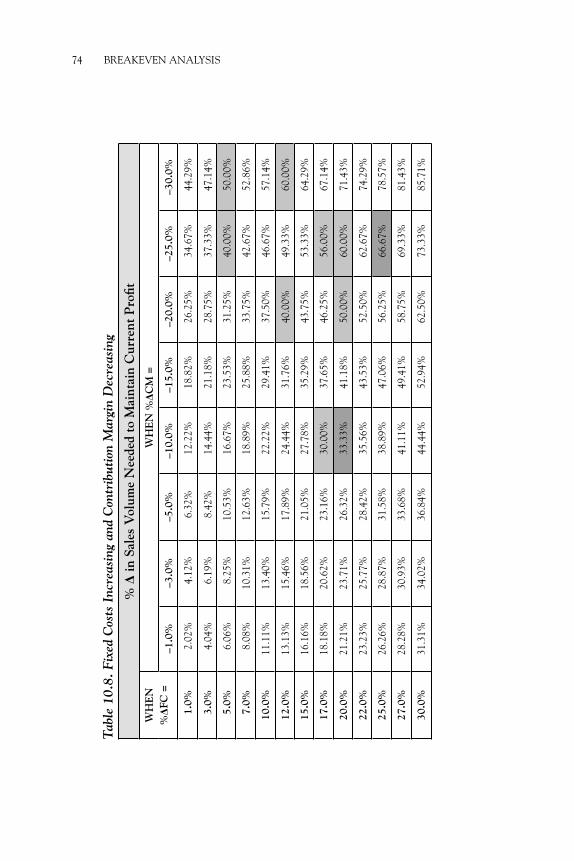
74 BREAKEVEN ANALYSIS
Tab
le 1
0.8.
Fix
ed C
osts
Inc
reas
ing
and
Con
trib
utio
n M
argi
n D
ecre
asin
g
% D
in S
ales
Vol
ume
Nee
ded
to M
aint
ain
Cur
rent
Pro
fi tW
HE
N
%D
FC =
WH
EN
%D
CM
=
–1.0
%–3
.0%
–5.0
%–1
0.0%
–15.
0%–2
0.0%
–25.
0%–3
0.0%
1.0
% 2
.02%
4.1
2% 6
.32%
12.
22%
18.
82%
26.
25%
34.
67%
44.
29%
3.0
% 4
.04%
6.1
9% 8
.42%
14.
44%
21.
18%
28.
75%
37.
33%
47.
14%
5.0
% 6
.06%
8.2
5% 1
0.53
% 1
6.67
% 2
3.53
% 3
1.25
% 4
0.00
% 5
0.00
%
7.0
% 8
.08%
10.3
1% 1
2.63
% 1
8.89
% 2
5.88
% 3
3.75
% 4
2.67
% 5
2.86
%
10.0
%11
.11%
13.4
0% 1
5.79
% 2
2.22
% 2
9.41
% 3
7.50
% 4
6.67
% 5
7.14
%
12.0
%13
.13%
15.4
6% 1
7.89
% 2
4.44
% 3
1.76
% 4
0.00
% 4
9.33
% 6
0.00
%
15.0
%16
.16%
18.5
6% 2
1.05
% 2
7.78
% 3
5.29
% 4
3.75
% 5
3.33
% 6
4.29
%
17.0
%18
.18%
20.6
2% 2
3.16
% 3
0.00
% 3
7.65
% 4
6.25
% 5
6.00
% 6
7.14
%
20.0
%21
.21%
23.7
1% 2
6.32
% 3
3.33
% 4
1.18
% 5
0.00
% 6
0.00
% 7
1.43
%
22.0
%23
.23%
25.7
7% 2
8.42
% 3
5.56
% 4
3.53
% 5
2.50
% 6
2.67
% 7
4.29
%
25.0
%26
.26%
28.8
7% 3
1.58
% 3
8.89
% 4
7.06
% 5
6.25
% 6
6.67
% 7
8.57
%
27.0
%28
.28%
30.9
3% 3
3.68
% 4
1.11
% 4
9.41
% 5
8.75
% 6
9.33
% 8
1.43
%
30.0
%31
.31%
34.0
2% 3
6.84
% 4
4.44
% 5
2.94
% 6
2.50
% 7
3.33
% 8
5.71
%

Chapter 11
Changing prices
Costs are not the only item that can change, making the work of a man-ager challenging. Companies can go along quite comfortably for weeks or months on track to achieve their annual profit goals. Sometimes without warning, competitors take an action or customers begin to change their tastes, requiring managers to consider changing selling price.
The application of breakeven analysis reviewed here seeks to answer this simple question: How would a selling price change affect sales goals and still generate equal or better profit?
This application of breakeven analysis takes as a given that the current level of profit is acceptable to managers. The application is built on the ratio of the change in selling price to contribution margin. Fixed costs and variable costs are assumed to remain unchanged in the short run. To help us with this situation, Smith and Nagle1 offer a useful formula to find the answer:
% Change in Sales Volume Needed = –Change in Price ÷
(Contribution Margin + Change in Price).
Using algebra notation we can simplify this with the following:
%D Sales = –DP ÷ (CM + DP),
where
%D Sales = % Change in Sales Volume Needed to Generate Equal Profit
DP = Change in Price (Measured in Dollars)
CM = Contribution Margin (in Dollars).
Assuming the variable costs do not change as a result of the price change, this formula calculates the minimum percent change in sales volume at the new price needed to generate the same level of profit. But price can

76 Breakevenanalysis
go up or down. When price goes down, the worry is whether enough sales volume will be generated to achieve the desired profit. When price goes up, the worry becomes whether too many customers will go away to achieve the desired profit.
Recall from economic theory that price decreases are expected to result in a percent increase in sales volume. Thus, under conditions of a pro-posed price reduction, the formula shows the minimum percent increase in sales needed to achieve the current profit.
Price increases are expected to result in a percent decrease in sales vol-ume. But in many cases the precise responsiveness of customers is not known. Thus, the formula shows the maximum percent decrease in sales that can be tolerated and still generate the same level of profit that the company enjoys before the price change. Managers are required to make a judgment regarding the likelihood of the decrease in sales occurring as a result of a price change.
example 1
Olympia Vacuum, Inc., sells 400,000 vacuum cleaners annually for total sales revenue of $24,000,000. That’s $60 per vacuum. Because sales were beginning to slow compared with this time last year, the marketing man-ager proposed decreasing the price by 5% from $60 to $57 per unit. The proposed change in price is just $3. He argued that this would give retail-ers the opportunity to either keep the retail price the same or decrease the price to capture more sales. The general manager said, “Fine. But before we implement the new price policy, I need to know the impact on sales that we should expect.”
Unit Variable Costs = $40 per Vacuum
Contribution Margin = ($60 – $40) = $20
The minimum percent increase in sales volume needed to maintain the same level of profit after the 5% price reduction is as follows:
%D Sales Volume Needed = –DP / (CM + DP)
= 3/(20 – 3)
= 3/17
= 17.65%

ChangingPriCes 77
In this case a little over 17% increase in sales volume is needed to main-tain the same level of profit after the price reduction.
example 2
Eagle Cap Wilderness Bikes sells 2,000 high-impact elite racing moun-tain bicycles for total sales revenue of $19,000,000. There is so much demand for the bikes that the marketing manager recommends to the general manager that the price be increased by 15%. She argues that the scarcity of the bikes coupled with the increase in price would strengthen the brand’s power with elite riders who seek a competitive edge and who are willing to pay almost any reasonable price for this advantage. The general manager of Eagle Cap says, “Let’s say that what you assume is correct regarding customer price sensitivities. Though frankly I doubt customers are that insensitive to a price increase. Don’t forget there are other really good race-quality mountain bikes on the market. And don’t confuse a spike in customer interest with normal interest through the rest of the year. Before we implement the new price policy, I need to know the impact on sales that we should expect. Specifically, what percent change in sales volume can we tolerate on the off-chance that sales decline with the price increase.”
Unit variable costs for these ultra lightweight but durable bikes equal $3,450. Unit selling price is $9,500. This makes the contribution margin a hefty $6,050—potentially a high-profitability product.
Since the marketing manager is proposing a price increase, normally we should expect a decrease in sales volume (unless this particular product is truly creating customers who are less responsive to price changes). The maximum change in sales that Eagle Cap Wilderness Bikes can tolerate with the price increase of 15% is as follows:
%D Sales Volume Tolerated = –DP / (CM + DP)
= –$1,425 / ($6,050 + $1,425)
= –19.06%
Changing prices also affect services. For example, the Red River Padres minor league baseball team sells tickets to its home games at $6 each. The stadium seats 1,500 fans. At the typical home game the ballpark is at 80% of capacity. The owner of the team estimates that the team incurs

78 Breakevenanalysis
$0.95 in variable costs at each home game. This leaves a contribution margin of $5.05 on each ticket sold. The Padres’ publicity manager sug-gests to the owner that the team should consider a special promotion by selling tickets at just $4 for one home game to see if this will pump up attendance.
The owner asks how many additional tickets need to be sold if the price is reduced for the special event. Because of the price reduction, con-tribution margin for each ticket will drop to $3.05 per ticket sold.
The minimum additional ticket sales needed to maintain the same level of profit after the price decrease are as follows:
%D Sales Needed = –DP / (CM + DP)
= –(–$2) ÷ ($5.05 – $2)
= $2 ÷ $3.05
= 65.57%
Rounding this, we might say under the conditions proposed by the pub-licity manager a 66% increase in ticket sales will be needed to achieve the current level of profit.
While the owner was calculating this figure, the publicity manager also suggested that every fan attending the special promotional game be given a sparkler firework valued at $0.25. These fireworks would be used after the game in center field as part of the fireworks extravaganza.
Upon hearing this additional detail, the owner continued calculating. When he was finished, he looked up and simply said, “Are you crazy? If we cut the price but do not give away sparklers, we will need at least a 66% increase in attendance to achieve our current per-game profit. But if we then increase the variable costs by 25 cents to put a sparkler in every ticket holder’s hot little hand, we’d need to add another 5.2% to the number of tickets sold to maintain our profit. This would put required attendance over the maximum available capacity by well over 500 ticket holders. What I’d like to know is where are you are going to put these 500+ people who don’t have seats so we can make our profit? Are they supposed to bring their own chairs?”

ChangingPriCes 79
an alternative approach and a Useful table
Former Purdue University professor John Tse2 offered an alternative approach to solving this problem. When a price reduction is contem-plated, such as when managers want to stimulate increased demand for products, someone needs to sell more units of the product in order to achieve the same profit level.
Tse’s formula is as follows:
DV% = [Ds% ÷ ((100 – v%s1) – Ds%)] × 100,
where
DV% = Minimum Increase in Sales Volume
(Expressed as Percentage of Breakeven
Sales Volume Before Price Change)
S1 = Selling Price Before Price Reduction
Ds% = Reduction in Selling Price (Expressed as
Percentage of Selling Price Before Price
Reduction)
v%s1 = Variable Cost (Expressed as Percentage
of Selling Price Before Price Reduction).
example 3
To use our previous example, Olympia Vacuum, Inc., is making a profit by selling its vacuums at $60 per unit. The sales director recommends a 30% reduction in selling price in order to be competitive in the market. The chief financial officer wants to know what percent additional sales volume will be needed to maintain the company’s current profit. Assume that the unit variable cost is 33.3% of the current selling price. If we also assume that everything else will remain unchanged in the company’s cost structure, we can use Tse’s formula to calculate the answer as follows:
DV% = [30 ÷ ((100 – 33.33) – 30)] × 100
DV% = 82%.

80 Breakevenanalysis
This means that if the price is reduced by 30%, the sales team will need to generate an increase of 82% of current sales volume. If the current volume that generates the desired profit is 75,000 units, the new sales volume will be
75,000 × 1.82 = 136,000 Units.
Changing prices and Variable Costs
But changing price is sometimes accompanied by changes in unit variable costs. Using his formula, Tse presented a useful table that allows a man-ager at a glance to estimate the percent change in sales volume needed to achieve current level of profits when both selling price (reduction) and unit variable costs (increase) change in an unfavorable direction. Tse pub-lished his table decades ago, but it has gotten lost in the shuffle of advanc-ing knowledge. We reproduce it here to help the busy manager (see Table 11.1).
One other type of change that should be considered is the prospect that fixed costs also change. When these change, there is an immediate impact on the breakeven point. To this we turn next.

ChangingPriCes 81
Tab
le 1
1.1.
Ada
pted
Fro
m T
se’s
Tab
le fo
r F
indi
ng th
e M
inim
um I
ncre
ase
of S
ales
Vol
ume
Req
uire
d to
Acc
ompa
ny
Sele
cted
Pri
ce R
educ
tions
to M
aint
ain
the
Pro
fit P
ositi
on B
efor
e P
rice
Red
uctio
n U
nder
Sel
ecte
d C
ost-
Pri
ce S
truc
ture
s
per
cent
incr
ease
in s
ales
req
uire
d to
mai
ntai
n cu
rren
t pr
ofit
%P
riC
eC
ha
ng
ev
ar
iaB
leC
ost
sa
s%
of
sell
ing
Pr
iCe
Bef
or
ePr
iCe
red
uC
tio
n
10.0
020
.00
30.0
040
.00
50.0
060
.00
70.0
080
.00
90.0
0
1.00
1.12
%1.
27%
1.45
%1.
69%
2.04
%2.
56%
3.45
%5.
26%
11.1
1%
3.00
3.45
%3.
90%
4.48
%5.
26%
6.38
%8.
11%
11.1
1%17
.65%
42.8
6%
5.00
5.88
%6.
67%
7.69
%9.
09%
11.1
1%14
.29%
20.0
0%33
.33%
100.
00%
7.00
8.43
%9.
59%
11.1
1%13
.21%
16.2
8%21
.21%
30.4
3%53
.85%
233.
33%
10.0
012
.50%
14.2
9%16
.67%
20.0
0%25
.00%
33.3
3%50
.00%
100.
00%
loss
*
15.0
020
.00%
23.0
8%27
.27%
33.3
3%42
.86%
60.0
0%10
0.00
%30
0.00
%
17.0
023
.29%
26.9
8%32
.08%
39.5
3%51
.52%
73.9
1%13
0.77
%56
6.67
%
20.0
028
.57%
33.3
3%40
.00%
50.0
0%66
.67%
100.
00%
200.
00%
loss
25.0
038
.46%
45.4
5%55
.56%
71.4
3%10
0.00
%16
6.67
%50
0.00
%
27.0
042
.86%
50.9
4%62
.79%
81.8
2%11
7.39
%20
7.69
%90
0.00
%
30.0
050
.00%
60.0
0%75
.00%
100.
00%
150.
00%
300.
00%
loss
33.0
057
.89%
70.2
1%89
.19%
122.
22%
194.
12%
471.
43%
35.0
063
.64%
77.7
8%10
0.00
%14
0.00
%23
3.33
%70
0.00
%
36.0
066
.67%
81.8
2%10
5.88
%15
0.00
%25
7.14
%90
0.00
%
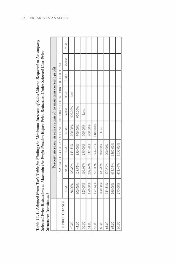
82 Breakevenanalysis
Tab
le 1
1.1.
Ada
pted
Fro
m T
se’s
Tab
le fo
r F
indi
ng th
e M
inim
um I
ncre
ase
of S
ales
Vol
ume
Req
uire
d to
Acc
ompa
ny
Sele
cted
Pri
ce R
educ
tions
to M
aint
ain
the
Pro
fit P
ositi
on B
efor
e P
rice
Red
uctio
n U
nder
Sel
ecte
d C
ost-
Pri
ce
Stru
ctur
es (
cont
inue
d)
per
cent
incr
ease
in s
ales
req
uire
d to
mai
ntai
n cu
rren
t pr
ofit
%P
riC
eC
ha
ng
ev
ar
iaB
leC
ost
sa
s%
of
sell
ing
Pr
iCe
Bef
or
ePr
iCe
red
uC
tio
n
10.0
020
.00
30.0
040
.00
50.0
060
.00
70.0
080
.00
90.0
0
40.0
080
.00%
100.
00%
133.
33%
200.
00%
400.
00%
loss
45.0
010
0.00
%12
8.57
%18
0.00
%30
0.00
%90
0.00
%
50.0
012
5.00
%16
6.67
%25
0.00
%50
0.00
%lo
ss
54.0
015
0.00
%20
7.69
%33
7.50
%90
0.00
%
55.0
015
7.14
%22
0.00
%36
6.67
%11
00.0
0%
60.0
020
0.00
%30
0.00
%60
0.00
%lo
ss
63.0
023
3.33
%37
0.59
%90
0.00
%
65.0
026
0.00
%43
3.33
%13
00.0
0%
66.0
027
5.00
%47
1.43
%16
50.0
0%

ChangingPriCes 83
Tab
le 1
1.1.
Ada
pted
Fro
m T
se’s
Tab
le fo
r F
indi
ng th
e M
inim
um I
ncre
ase
of S
ales
Vol
ume
Req
uire
d to
Acc
ompa
ny
Sele
cted
Pri
ce R
educ
tions
to M
aint
ain
the
Pro
fit P
ositi
on B
efor
e P
rice
Red
uctio
n U
nder
Sel
ecte
d C
ost-
Pri
ce
Stru
ctur
es (
cont
inue
d)
per
cent
incr
ease
in s
ales
req
uire
d to
mai
ntai
n cu
rren
t pr
ofit
%P
riC
eC
ha
ng
ev
ar
iaB
leC
ost
sa
s%
of
sell
ing
Pr
iCe
Bef
or
ePr
iCe
red
uC
tio
n
10.0
020
.00
30.0
040
.00
50.0
060
.00
70.0
080
.00
90.0
0
70.0
035
0.00
%70
0.00
%lo
ss
72.0
040
0.00
%90
0.00
%
75.0
050
0.00
%15
00.0
0%
80.0
080
0.00
%lo
ss
81.0
090
0.00
%
85.0
017
00.0
0%
90.0
0lo
ss
*Los
s m
eans
that
the
selli
ng p
rice
dro
pped
bel
ow th
e va
riab
le c
ost,
caus
ing
a lo
ss o
n th
e sa
le o
f eve
ry u
nit.
Whe
n th
is o
ccur
s, y
ou c
anno
t “m
ake
up th
e di
ffer
ence
” by
sel
ling
mor
e! T
he m
ore
you
sell,
the
mor
e yo
u lo
se.
Sour
ce.
Tse,
Joh
n Y.
D. (
1960
). P
rofit
pla
nnin
g th
roug
h vo
lum
e-co
st an
alys
is. N
ew Y
ork:
Mac
mill
an. p
. 83.
Use
d w
ith
perm
issi
on.


Chapter 12
Selling price at Various Volumes
Bob, the appliance retailer, recently saw an ad for a competitor appliance store. The competitor was offering to sell a refrigerator for substantially less than Bob’s price. Bob wondered, “We are selling identical refrigera-tors. How can they sell them for so much less and still make a profit?”
Assume Bob’s Appliances sells only refrigerators (a simplifying assumption). We have the information shown in Table 12.1, Impact of Changing Volume.
To answer Bob’s question, there are three changes that would allow a lower selling price:
1. As shown in Table 12.1, selling a larger volume of units would spread the fixed costs over more units and reduce the fixed cost per unit.
2. Total fixed costs could be reduced, which would reduce the fixed cost per unit. Suggestions for reducing total fixed costs could include reduced rent (a less expensive store or a smaller store), becoming more energy efficient, and shopping for a lower premium on business insurance.
3. Accepting a lower desired profit would allow Bob to reduce his selling price.
Next, let’s consider a different business environment and the manage-ment concept of target costing.
Have you ever wondered how the price of a product can drop dra-matically after the product has been on the market for a while? The vid-eocassette recorder (VCR), introduced to consumers around 1980, sold for about $1,000. Twenty years later, a VCR sold for perhaps 10% of

86 Breakevenanalysis
the original 1980 selling price. There are a number of reasons, but we will focus on two: (a) the increase in the quantity of units sold and (b) the reduction of variable costs per unit. Assume the data in Table 12.2, Impact of Changing Volume and Variable Costs.
Between 1980 and 2000, two obvious things happened. First, the sales demand increased greatly. That allowed the producer to spread the fixed costs and desired profit over many more units and reduced the contribution margin needed per unit from $400 in 1980 to only $30 in 2000. The hefty reduction in total required contribution margin allowed the producer to significantly reduce the per-unit selling price while con-tinuing to earn the same total profits.
Second, the variable cost per unit declined dramatically, from $600 per unit in 1980 to $70 per unit in 2000. This cost reduction may be
Table 12.2. Impact of Changing Volume and Variable Costs
Year 1980 2000annualfixedcosts(FC) $5,000,000 $5,000,000
annualdesiredprofit(DP) $1,000,000 $1,000,000
Totalcontributionmargin(CM=FC+DP) $6,000,000 $6,000,000
salesdemand(units)(sU) ÷15,000 ÷200,000
Contributionmarginperunit(CMU=CM÷sU) $400 $30
variablecostperunit(vCU) $600 $70
sellingpriceperunit(sPU=CMU+vCU) =$1,000 =$100
Table 12.1. Impact of Changing Volumeannualvolumeofrefrigeratorssold 500 1,000 1,500
annualfixedcosts(FC) $437,500 $437,500 $437,500
annualdesiredprofit(DP) $100,000 $100,000 $100,000
Totalcontributionmargin(CM=FC+DP) $537,500 $537,500 $537,500
annualsalesvolume(units)(sU) ÷500 ÷1,000 ÷1,500
Contributionmarginperunit(CMU=CM÷sU)
$1,075 $537.50 $358.33
variablecostperunit(vCU) $650 $650 $650
sellingpriceperunit(sPU=CMU+vCU)
=$1,725 =$1,187.50 =$1,008.33

sellingPriCeaTvarioUsvolUMes 87
credited to cheaper materials, low-cost labor in third-world countries, and innovations in the production process. But these cost reductions were driven by a shift in management thinking. Traditional cost-plus pricing (illustrated in the 1980 VCR example) accumulated all costs, added a desired profit, and magically arrived at the “right” selling price.
Target costing is a reversal of the thinking in traditional cost-plus price setting. Target costing first determines through market research an appropriate selling price per unit and volume of units that can likely be sold. Management then sets the desired profit (per unit or in total). Finally, the difference between the selling price and the desired profit is the cost the company can afford to spend to produce and sell the product. At this point, engineers from research and development and personnel from materials acquisition, human resources, and produc-tion team up to find a way to make the product at or below the target cost.1


Chapter 13
Multiple Breakeven points
Because of unpredictable student enrollment, the local community col-lege leases classroom space and hires adjunct professors to teach multiple sections of introductory English and mathematics courses. The college requires that each course section taught have a minimum of 6 and a max-imum of 25 students.
The scenario in the preceding paragraph introduces the interesting possibility that an organization may break even at more than one volume of sales. Whenever an organization’s fixed costs change, the breakeven point changes. Fixed costs, in the community college example, would be classroom leases and adjunct professor salaries. For the college, the relationship is a circular one. If more students enroll, the college must hire more adjunct professors. If the college hires more adjunct professors, its fixed costs and its breakeven point rise, requiring more students to enroll. Observe in the following example how the breakeven point moves upward as student enrollment increases.
Assume the following data shown in Table 13.1, Community College Selected Costs and Prices.
One section taught will be the unit of measure. We need to calculate the contribution margin per section taught. Each section will be filled to its maximum of 25 students before another section is offered.
Table 13.1. Community College Selected Costs and PricesStudent tuition per course $120
Instructional supplies per student per course $20
Adjunct professor salary per course section taught $2,100
Leased building for eight classrooms per semester $2,000

90 BreAkeven AnALySIS
Tuition Revenue per Section = ($120 × 25 Students) = $3,000
Variable Costs for Instructional Supplies per Section =
($20 × 25 Students) = $500
Variable Cost of Professor’s Salary per Section = $2,100
Contribution Margin per Section = ($3,000 – $500 – $2,100) = $400
Let’s calculate the breakeven point:
$2,000 Fixed Cost (Lease)=
5 Units (Sections to
Be Taught).$400 per Section Contribution Margin
The community college must have five sections filled with the maximum number of students to reach breakeven.
Now, let’s consider the surprising results of different numbers of students enrolling shown in Table 13.2, Profit and (Loss) at Different Enrollments.
How can it be that the college breaks even at two points (125 stu-dents enrolled and 167 students enrolled), while it earns a profit with only 147 students enrolled, but loses money with 157 students enrolled? The answer lies in the concept of the relevant range. Every time student enrollment exceeds the maximum of 25 students per classroom, enroll-ment exceeds the relevant range, so capacity must increase (an additional professor must be hired to teach an additional section). This increase in
Table 13.2. Profit and (Loss) at Different EnrollmentsStudent enrollment 125 147 157 167
Course sections 5 6 7 7
Tuition revenue $15,000 $17,640 $18,840 $20,040
variable cost supplies $2,500 $2,940 $3,140 $3,340
Salaries $10,500 $12,600 $14,700 $14,700
Lease $2,000 $2,000 $2,000 $2,000
Profit (Loss) $0 $100 ($1,000) $0

MuLTIPLe BreAkeven PoInTS 91
capacity increases the fixed costs incurred and, consequently, changes the breakeven point. Let’s calculate the breakeven student enrollment for six sections taught.
$14,600 Fixed Costs (Salaries + Lease)= 146 Students
$100 per Student Contribution Margin
Recalling that initial breakeven was at five sections, if the college decides to open a sixth section, it needs to be reasonably sure of obtaining between 146 and 150 students to cover all its costs. If student enrollment rises above 150 students, the college must open a seventh section.
If the college offers seven course sections, the breakeven point would be
$16,700 Fixed Costs (Salaries + Lease)= 167 Students.
$100 per Student Contribution Margin
If potential enrollment exceeds 150 students, so that a seventh section is needed, the college needs to attract at least 167 students to cover all its costs.
The preceding example has illustrated multiple breakeven points when sales volume rises. The same concepts and methods apply when sales volume declines if the organization is able to reduce its capacity (fixed costs). In the college or university environment, if the additional profes-sors hired were tenured professors instead of adjunct professors, then the educational institution would not be able to reduce its fixed costs and, therefore, would not be able to reduce its breakeven point.
Readers who are interested in a more mathematical approach to ana-lyzing business scenarios with multiple breakeven points are referred to the discussion of the quadratic equation in chapter 15.


Chapter 14
Net present Value Method
Net present value (NPV) is one of a group of topics often referred to as capital budgeting. It isn’t often viewed as a cost-volume-profit technique. In this method, we will calculate a cost or a value, which we will call the indifference point. Typically, an organization is faced with deciding between two alternatives, each of which will have the same result to the organization (hence, the indifference). Sometimes, one application of this method is called the outsource decision (or the make-or-buy decision).
Let’s get started with an example.
example 1
Statewide Industries currently has a landscaping department to care for the vast, tastefully decorated grounds surrounding its office and labora-tory complex. Statewide has just received a proposal from a landscap-ing contractor that, if accepted, would outsource the landscape work and eliminate the current landscaping department. So the company’s choices are (a) to continue doing its own work in house or (b) to outsource the work to the contractor. The landscaping department’s equipment is gen-erally old, worn out, or obsolete. This is an ideal time for the company to consider whether to replace all the equipment or outsource. Table 14.1 gives Statewide Industries data. Table 14.2 gives the indifference point calculation steps.
If the outsource company were to bid $166,197, the company would break even on the work done. That is, either choice would end up costing the company exactly the same over the 7-year period.
Any outsource contractor’s bid above this indifference amount is too high and should not be accepted. If an outsource contractor’s bid is below this indifference amount, then outsourcing will reduce the organization’s total costs. With an indifference point of $166,197, if the outsource

94 Breakevenanalysis
contractor were to bid to do the work for $164,000 annually, Statewide Industries would save $2,197 ($166,197 – $164,000) annually by accept-ing the offer and eliminating the in-house department.
There are at least two additional complicating factors that, while real-istic, are beyond the intended scope of this book. Most profitable compa-nies would use Modified Accelerated Cost Recovery System depreciation instead of straight-line depreciation. This change in depreciation method would generally favor the in-house choice and require a lower outsource bid to be indifferent.1 Because the topic of depreciation is a complex one, the reader is encouraged to consult with a tax professional.
We have also disregarded the effect of inflation on either the in-house operating costs or the outsource contractor’s price over the multiple-year period being evaluated.2
Table 14.2. Indifference Point Calculation Stepsequipmentacquisitioncost $84,000
Dividedbypresentvalueofa7-yearannuityat16% ÷ 4.038
equalsannualoperatingcashflowatindifferencepoint $20,802
subtractannualdepreciation – $12,000
equalsnetincomeeffectatindifference $8,802
Dividedby(1–taxrateasadecimal;1–.38) ÷ 0.62
equalspretaxsavingstodoworkinhouseatindifference =$14,197
addannualin-housecosts($140,000+$12,000depreciation) + $152,000
equalsindifferencepoint =$166,197
Table 14.1. Statewide Industries Dataequipmentacquisitioncost $84,000
straight-linedepreciation
7-yearlife
replacementequipmenthasnoresidualvalue
annualdepreciation($84,000÷7years) $12,000
annualoperatingcosts(labor,equipmentrepair,etc.) $140,000
Contractor’sbidtoperformalllandscapework(annualcost) $175,000
Currentlyusedequipmenthasnoresidualvalue
CombinedFederalandstateincometaxrate 38%
Costofcapital 16%

netPresentvalueMethoD 95
Breakeven and the Cost of Capital
The economic view of the firm leads managers to earn something more than accounting profit in order to generate a return to the owners large enough to offset what the owners could have earned by engaging in some other similar-risk investment. This additional amount of profit is usually discussed in terms of the opportunity cost of capital.
The time value of money theory teaches us that the true breakeven point that considers the opportunity cost plus all other costs will always raise the true total cost, which, in turn, will always raise the breakeven point.
To see an example of factoring in opportunity cost, consider a manu-facturing enterprise that makes and sells do-it-yourself home painting equipment. To show the impact of the opportunity cost on the breakeven point, we will first calculate the breakeven point using the traditional approach and then follow up by incorporating the cost of capital into the calculation using a method presented by Brealey, Myers, and Marcus.3
example 2
PowerRoll’s most popular product, which represents over 95% of its sales, is its power paint roller on a long handle that pumps paint out of a bucket, up the long handle, and into the roller, helping the painter be more efficient. Their paint roller sells for $25 to hardware stores. Unit variable costs total $12. During one relevant time period the firm sold 21,000 paint rollers through a regional network of neighborhood hard-ware stores. This earned gross revenues of $525,000. If the firm’s fixed costs equal $310,000, the breakeven point is calculated as follows:
BEU = FC ÷ CM
U
BEU = $310,000 ÷ ($25 – $12) = $310,000 ÷ $13 = 23,846 Units.
The sale of 21,000 units is below the breakeven point.Managers at PowerRoll are considering the possibility of purchasing a
new $100,000 piece of equipment that has the potential of lowering the unit variable cost from $12 to $10. For now we can assume that the com-pany should be able to sell at least as many rollers in each of the coming years as they have recently. But adding the new equipment will increase

96 Breakevenanalysis
the fixed costs by $20,000, bringing total fixed costs up to $330,000. Half of this increase in fixed costs will be depreciation. By using the new equipment, managers expect unit variable costs to decrease. The new breakeven point can be calculated as follows:
BEU = FC ÷ CM
U
BEU = $330,000 ÷ ($25 – $10) = $330,000 ÷ $15 = 22,000 Units.
The fixed costs will increase, but managers also expect the unit contribu-tion margin to increase. The net effect is that managers at PowerRoll will find it a little easier to achieve breakeven even though the fixed costs have increased. This illustrates how powerful changes in variable costs can be to lower the breakeven point even under conditions where the fixed costs are increasing.
Spreading the depreciation of the new equipment over 10 years using the straight-line method, the depreciation expense of the new equipment will be $10,000 per year. After the capital investment, annual deprecia-tion will be $10,000.
Table 14.3, PowerRoll Data, is a summary of the business model ele-ments we have established thus far after taking into consideration the capital investment and total annual depreciation expense.
We can rewrite this data into an algebra format that puts us on the road to solving for the number of units (q) needed to be sold per year to break even. These data are shown in Table 14.4, Algebraic Format of PowerRoll Data.
To calculate net cash flow, we add the $10,000 in depreciation expense:
Annual Cash Flow = 9.9q – $207,800.
Table 14.3. PowerRoll DataCapitalinvestment $100,000
unitsaleprice $25
unitvariablecost $10
Depreciation $10,000
otherfixedcosts $320,000
totalfixedcosts $330,000

netPresentvalueMethoD 97
To find the present value of net cash flow, we multiply net cash flow by an annuity factor. The annuity factor operates like net present value in that it helps determine the annual amount of opportunity cost of capi-tal on an investment spanning 10 years at 7% discount rate. To deter-mine the annuity factor, we consult an annuity table for the interest rate per year and the number of years for which the investment is being analyzed (see Appendix E). Alternatively, we can use an annuity formula, which can be found in most business finance books or on the Internet. The appropriate annuity factor for this example is 7.024.
Applying the annuity factor we get the following:
Annual Cash Flow Discounted by 7% Over 10 Years =
7.024 (9.9q – $207,800).
Now we must account for the $100,000 investment, which is negative cash flow, by placing it in the formula as follows to obtain net cash flow:
Net Cash Flow = –$100,000 + 7.024 (9.9q – $207,800).
Setting the equation to zero and solving for q, we obtain the number of units to break even:
0 = –$100,000 + 7.024 (9.9q – $207,800)
0 = –$100,000 + 69.5376q – $1,459,587.20
0 = 69.5376q – $1,559,587.20
69.5376q = $1,559,587.20
q = $1,559,587.20 ÷ 69.5376 = 22,428
(Rounded Up to Next Whole Unit).
Table 14.4. Algebraic Format of PowerRoll Datatotalsalesrevenue $25q
totalvariablecosts $10q
Depreciation $10,000
totalfixedcosts $330,000
Pretaxprofit 15q–$330,000
taxesat34% 5.1q–$112,200
netprofit 9.9q–$217,800

98 Breakevenanalysis
The 7% discount rate is an estimate of the risk the firm faces as it attempts to use its resources to generate future cash flow over time through its busi-ness operations. We can estimate the firm’s risk by using an approach such as the capital asset pricing model (CAPM), the weighted average cost of capital (WACC), the degree of operating leverage, or a more conservative approach using the risk-free rate of return4 such as what might be earned from investing in Treasury bills. These are methods described in finance books, which we won’t take the time to review here. The 10-year time period is a somewhat arbitrary number of years that managers expect to generate a return over the life of the equipment purchased and used.
The traditional accounting method to calculate breakeven determines that PowerRoll needs to sell 22,000 units. The breakeven method we are exploring here indicates that 22,428 units need to be sold to cover all costs including the cost of capital. Compare these two breakeven amounts in Table 14.5, Comparison of Breakeven Methods.
Table 14.6, Net Income at Economic Breakeven, shows the net income result of selling 22,428 units.
We can call the breakeven point the economic breakeven since it attempts to incorporate the opportunity costs of capital into the calculation.
Table 14.5. Comparison of Breakeven Methods
Breakeven using traditional method
Breakeven factoring in opportunity cost
Difference Difference
22,000units 22,428units 428units 1.9%
Table 14.6. Net Income at Economic BreakevenGrosssales(22,428powerpaintrollers) $560,700
lesstotalvariablecostsat$10each $224,280
Contributionmargin $336,420
lessfixedcosts $330,000
netincomebeforetaxes $6,420

netPresentvalueMethoD 99
Observations
One observation we can make is that as risk increases and everything else remains unchanged, the economic breakeven point also will increase and as this increases the difference between the accounting method and the economic method is greater.
Economic breakeven method generates a result that is higher than the traditional accounting breakeven method, assuming that the length of the depreciation period is equal to the length of the investment period. As fixed costs increase or as the annuity factor increases, the difference between the two methods of calculation will decrease but will never be precisely equal.
As in other examples we have given in this book, the economic break-even point must be considered in the context of actual operating condi-tions. Company operations managers must ask themselves whether the enterprise has the operational capacity to produce the number of units required to achieve economic breakeven. For example, what adjust-ments might be necessary in terms of scheduling personnel and materi-als, machine use, maintenance, and outbound logistics? Does sufficient operational slack exist that allows the firm to ramp up production? In some companies, increasing the production may not be possible given the current configuration of assets.
The sales team also must make some judgments regarding the level of demand that can reasonably be stimulated by their efforts in order to achieve economic breakeven. To stimulate this level of demand, will price concessions need to be entertained or will geographic expansion of sales efforts be required and at what additional cost? Estimates of additional costs that might be incurred to produce and sell the economic breakeven amount should be factored into the breakeven calculation.
Variations to the Method
A variation on this, which yields an estimate that is identical to that obtained in the previous analysis, is to take the annual net cash flow and compare it with the amount needed to pay for the annual cost equivalent of the investment when discounted by an annuity factor.5 This approach treats the payback to the investment as if the company

100 Breakevenanalysis
had to earn enough cash to pay an annuity to the shareholders each
year. The annual “payment” is the annual opportunity cost of the capi-
tal investment. Using a discount rate of 10% and a 10-year life of the
investment, we can use the annuity factor of 6.145 (from the annuity
formula or an annuity table) in the following equation:
Annual Opportunity Cost of Investment =
$1,000,000 ÷ 10-Year Annuity Factor
Annual Opportunity Cost of Investment =
$1,000,000 ÷ 6.145 = $162,745.
This means that over a 10-year period, in addition to covering all other
annual costs, the company must generate annually $162,745 in cash to
cover the cost of capital. This means that when the annual net cash flow from
the sale of products and the annual opportunity cost are equal, the firm has
broken even. Table 14.7, Sensitivity Analysis, illustrates that the
firm breaks even when it makes and sells 5,461 units.
The difference between the accounting approach to break even
and the interests of economics has been a subject of consideration for
decades.6 In addition to the methods reviewed here, there are other more
complex approaches that factor in the cost of capital.7 You might be inter-
ested in reviewing these sometime.
Weaknesses
The economic breakeven method may be considered superior to other
methods since it incorporates the time value of money over a period of
years. But this method is not perfect. This method implies that variable
costs and unit selling prices remain the same over time. One way to over-
come this weakness is to adjust the unit variable costs and unit selling
price by a reasonable factor such as inflation or other known benchmark.
In real life it is unlikely that unit selling prices and unit variable costs will
remain stable over several years. They may, in fact, change at different
rates.
Future cash flow may be difficult for some small companies to esti-
mate. Using depreciation as the only way to estimate cash flow implies
that no other cash flow influences are at work in the business. In reality,

netPresentvalueMethoD 101
Tab
le 1
4.7.
Sen
siti
vity
Ana
lysi
sD
isC
ou
nt
ra
te
(r)
0.10
uni
tsel
ling
pric
e$2
,500
$2,5
00$2
,500
$2,5
00$2
,500
uni
tvar
iabl
eco
st$1
,750
$1,7
50$1
,750
$1,7
50$1
,750
uni
tcon
trib
utio
nm
argi
n$7
50$7
50$7
50$7
50$7
50
uni
tsso
ld1,
000
3,00
05,
461
6,00
08,
000
tota
lrev
enue
$2,5
00,0
00$7
,500
,000
$13,
652,
500
$15,
000,
000
$20,
000,
000
tota
lvar
iabl
eco
st$1
,750
,000
$5,2
50,0
00$9
,556
,750
$10,
500,
000
$14,
000,
000
Fixe
dco
sts(
FC)
$4,0
00,0
00$4
,000
,000
$4,0
00,0
00$4
,000
,000
$4,0
00,0
00
Dep
reci
atio
n(i
nclu
ded
inF
C)
$100
,000
$100
,000
$100
,000
$100
,000
$100
,000
Pret
axp
rofit
($3,
250,
000)
($1,
750,
000)
$95,
750
$500
,000
$2,0
00,0
00
tax
at3
4%($
1,10
5,00
0)($
595,
000)
$32,
555
$170
,000
$680
,000
net
pro
fit($
2,14
5,00
0)($
1,15
5,00
0)$6
3,19
5$3
30,0
00$1
,320
,000
ann
ualn
etc
ash
flow
($2,
045,
000)
($1,
055,
000)
$163
,195
$430
,000
$1,4
20,0
00
ann
ualo
ppor
tuni
tyc
ost
on$
1Mo
ver1
0ye
arsa
t10%
$162
,745
$162
,745
$162
,745
162,
745
$162
,745
Diff
eren
ce(
netc
ash
flow
–a
nnua
lop
port
unit
yco
st)
($2,
207,
745)
($1,
217,
745)
$450
$267
,255
$1,2
57,2
55
102 Breakevenanalysis
accounts receivable and accounts payable also influence cash flow, but these are not taken into consideration with the method discussed previ-ously. The wise manager will track down all the various elements that drive cash flow in his or her particular business.
Annual cash flow 5 years from now may be generated from entirely different conditions than currently exist. The capital structure of the organization will likely be different 5 years from now. The NPV method implies that managers will not make adjustments to the business model as the organization proceeds into the future. Even with its weaknesses, one can argue that the traditional accounting method to calculate breakeven ignores the future even more than does the economic method!
Discounted future cash flows are sensitive to the discount rate, which may be difficult to identify for specific projects or particular businesses. Private companies may find it difficult to locate information on compa-rable companies and the discount rate that should apply.
ethical Considerations
For the manager whose task is to calculate and report the breakeven point, several ethical considerations should be addressed.8 For example, managers may attempt to unethically manipulate the outcome of the breakeven calculation in order to achieve some purpose other than find-ing the truth about breakeven, such as when trying to persuade top-level leaders to increase a capital investment. Ignoring the relevant range or treating some fixed costs as variable costs can manipulate the calculation. Distorting breakeven graphs so that an incorrect conclusion is drawn by the graph user is another way to manipulate the information unethically.
Studying the impact of economic needs of the firm brings into sharp relief one of the fundamental tensions that managers experience. Under-standing the breakeven point and the elements of the business model that contribute to breakeven helps a manager appreciate much more deeply the impact of day-to-day operational decisions on the firm’s ability to generate wealth. Thus, on one hand, managers want to make economi-cally sound decisions that are responsible to the shareholders. On the other hand, these managers want to make decisions that take into consid-eration fundamental duties owed to the greater good of society, as well as the decision’s impact on the greater good of society.

netPresentvalueMethoD 103
Ethical values go hand in hand with business values. For example, recognizing the potential harm that can come to a firm’s reputation or to one’s career when the firm takes advantage of others in order to earn an economic profit, the majority of managers are careful to obey the law and go beyond the letter of the law to do good at the same time as they are doing well economically.
Dynamic markets and regulations constrain managers, making it dif-ficult to achieve an economic profit. Under such constraints managers may be tempted to cut corners, use deceit, or commit fraud to make up for their inability to overcome these barriers.
In most instances, managerial decisions that result in achieving eco-nomic breakeven are not in conflict with ethical values. But we should recognize ethical values that managers prize can and do act as constraints on managerial decision making. Not just anything goes9 if we expect the market economy to continue working efficiently and our brands to main-tain strong consumer support. Managers must take into consideration not only the economic goals of the firm but also the greater good of society.
Cognizant of the importance of building shareholder wealth, some managers will choose not to squeeze every nickel and dime out of a com-pany’s business model to cover the true total costs when doing so means that they must compromise their ethical values or in other ways bring harm to the greater good of society. Taking the perspective that life does not consist solely in the abundance of possessions such as wealth-building assets, under some circumstances managers may be willing to forgo a por-tion of the economic profit for the sake of employees, other stakeholders such as customers, or the environment shared in common by society.


Chapter 15
Quadratic equation
It can be argued that when the relevant range is used, the traditional breakeven formula shows a relatively linear relationship between quan-tity and cost and revenue. The basic formula for breakeven analysis also assumes that the business situation is unchanging in terms of selling price, unit variable costs, fixed costs, product mix, and a host of other vari-ables that can affect both revenue and costs. Can we calculate breakeven when either the revenue curve or the cost curve is changing? For exam-ple, a company may face new competitors in the market that offer more choices for customers. These companies enter the market for the product because the investors believe they can capture cash value from customers if demand is on the increase. More companies entering the market tends to increase customer responsiveness to price changes (price elasticity of demand).
As customer responsiveness increases, it becomes increasingly diffi-cult to win new customers and keep current customers. The entrance of new competitors in the market usually results in incumbents reacting to this by lowering their prices. Lowering prices makes the revenue curve change as more units are produced and sold. Total revenue begins to decline as more and more units are sold. The cost curve may continue to be a linear relationship: Our variable costs are unchanged, and our fixed costs are the same.
If the revenue curve drops low enough (because we continue to lower prices), we could very well anticipate a time when we drop the price too low and sell units at a loss. If this occurs, we should expect to find two breakeven points, not just one. In practical terms, we will need to be as concerned about selling too many products if our prices get too low as we would be in attempting to sell enough products to break even.

106 Breakevenanalysis
Changes in revenue
Consider the following simple example of historical data from a company that makes an unusual type of MP3 player.1 See Table 15.1, Revenue and Costs. As more units are produced, competitors jump into the market and the market price declines.
Using a statistics software application or a spreadsheet application that contains statistical functions, we can determine the formulas for both the total revenue curve and the total cost curve. We can also graph this table using spreadsheet software.
For this example, the formulas for the two curves are as follows:
R(x) = (–x2 ÷ 1000) + 10x
Table 15.1. Revenue and Costs
x r(x) C(x)0 0 7,000
500 4,750 8,000
1,000 9,000 9,000
1,500 12,750 10,000
2,000 16,000 11,000
2,500 18,750 12,000
3,000 21,000 13,000
3,500 22,750 14,000
4,000 24,000 15,000
4,500 24,750 16,000
5,000 25,000 17,000
5,500 24,750 18,000
6,000 24,000 19,000
6,500 22,750 20,000
7,000 21,000 21,000
7,500 18,750 22,000
Where
x = Number of MP3 Players Produced and Sold
R(x) = Total Revenue
C(x) = Total Cost

QuadraticeQuation 107
C(x) = 7000 + 2x.
You may recall from high school algebra that the form the formula for R(x) takes is called a polynomial.
We know the breakeven point is the point where total revenue equals total cost, or
R(x) = C(x).
So we can substitute the two curve formulas in this equation as follows and solve for x since x is the number of units of our MP3 player that we are concerned about:
R(x) = C(x)
(–x2 ÷ 1000) + 10x = 7000 + 2x.
If we set this polynomial formula equal to zero, we get the following:
(–x2 ÷ 1000) + 8x – 7000 = 0.
You may remember from high school math class that the polynomial equation is known as the quadratic equation: ax2 + bx + c. To solve for x in a quadratic equation, we can use the famous quadratic formula:
x = –b± b2 – 4ac2a
In so doing, we come up with the following results:
x = 8,000 ± 6,000 ÷ 2
x = 1,000, x = 7,000.
As the graph (plotted using spreadsheet software) in Figure 15.1, Multiple Breakeven Points—Linear Cost Curve, shows, our two breakeven points are at 1,000 units and 7,000 units.
In practice, company decision makers will watch the impact of falling prices on the cost-volume-profit relationship. This graph shows that if the decision makers don’t do anything different except drop the price, they will reach the upper breakeven point at 7,000 units. If the market price contin-ues to drop, the company must either find a way to differentiate its product from that of competitors so it can keep its prices higher than what other

108 Breakevenanalysis
companies charge, or it must find ways to decrease its fixed costs, unit costs, or both. This illustrates why companies in highly competitive markets where the price elasticity of demand is changing (in an unfavorable direc-tion, i.e., increasing) and where opportunities to differentiate one company from another exert more effort to find ways to lower their costs. To main-tain profitability, they are being chased by the upper breakeven point!
Costs and revenue Changing
Depending on the specific situation, a company may also face the unsa-vory scenario in which both costs and revenue are changing in unfavor-able directions. By extending Barnett and Ziegler’s2 approach, we now have total revenue curve and the total cost curve nonlinear (changing) as illustrated in Figure 15.2, Nonlinear Cost and Revenue Curves.
This graph visually indicates that something unpleasant is happening to the company’s ability to grow its total revenue. In addition, unit vari-able costs are increasing rather than staying static. It could be that the supply of an important ingredient used in the product is decreasing, thus driving the cost of that ingredient ever higher. There could be other fac-tors that bring relatively rapid changes to the cost of production and dis-tribution such as energy costs. Consider Table 15.2, Changing Revenue and Costs, which was used to generate the graph.
0
5000
10000
15000
20000
25000
30000
R(×)
C(×)
Figure 15.1. Multiple Breakeven Points—Linear Cost Curve
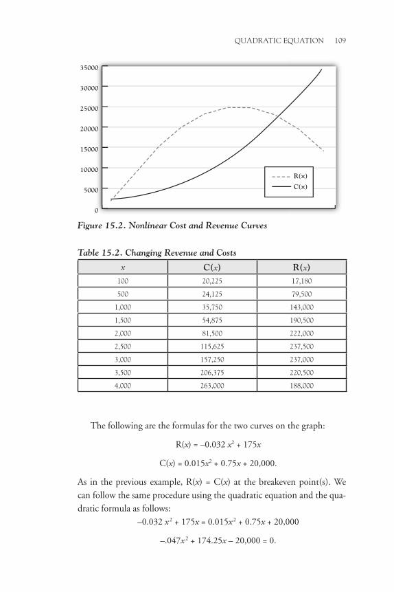
QuadraticeQuation 109
The following are the formulas for the two curves on the graph:
R(x) = –0.032 x2 + 175x
C(x) = 0.015x2 + 0.75x + 20,000.
As in the previous example, R(x) = C(x) at the breakeven point(s). We can follow the same procedure using the quadratic equation and the qua-dratic formula as follows:
–0.032 x 2 + 175x = 0.015x 2 + 0.75x + 20,000
–.047x 2 + 174.25x – 20,000 = 0.
0
5000
10000
15000
20000
25000
30000
35000
R(×)
C(×)
Figure 15.2. Nonlinear Cost and Revenue Curves
Table 15.2. Changing Revenue and Costs
x C(x) r(x)100 20,225 17,180
500 24,125 79,500
1,000 35,750 143,000
1,500 54,875 190,500
2,000 81,500 222,000
2,500 115,625 237,500
3,000 157,250 237,000
3,500 206,375 220,500
4,000 263,000 188,000

110 Breakevenanalysis
Using the quadratic formula to solve for x, we get the following:
x = (–174.25 + 161.104) / –0.094 = 140 Units (After Rounding)
x = (–174.25 – 161.104) / –0.094 = 3,568 Units.
Notice that if unit variable costs had remained unchanged, the upper breakeven point would be higher than it is when unit variable costs increase. On the following graph shown in Figure 15.3, Comparison of Breakeven Points, the dotted line represents unit variable costs that are linear (unchanging). Notice what happens to the breakeven point! It moves to the right.
In other words, as unit variable costs increase, the upper breakeven point decreases over what it might have been if unit variable costs had remained unchanged. If the company can work diligently to keep its unit variable costs stable (such as signing a long-term contract for a key factor used in production or distribution), it can weather the storm of decreas-ing market prices longer than its competitors can.
Interestingly, once we know the formula for the total cost curve and the total revenue curve, we can also calculate the production/sales level where profit is at its maximum.
0
5000
10000
15000
20000
25000
30000
35000
R(×)
C(×)
Figure 15.3. Comparison of Breakeven Points

QuadraticeQuation 111
Limitations
We know that the basic breakeven formula has serious limitations imposed
by the fairly severe assumptions required. Using polynomial equations to
estimate breakeven carries its own limitations. First, a polynomial curve
such as for total revenue assumes that total revenue will cross the zero line
at least twice. Of course, revenue is zero before any units are sold. But at
the upper end of the curve, crossing zero usually will occur only when
the firm stops selling products. In other words, the polynomial equation
may not hold true at the upper end of the curve if the company deci-
sion makers respond to their environment by cranking up advertising to
stimulate demand, coming out with different products that reinvigorate
the revenue curve. Likewise, the polynomial total cost curve assumes that
total costs will continue to rise infinitely. While it feels like this is hap-
pening in volatile markets, company decision makers normally will make
adjustments to keep infinite costs from being incurred.
A second weakness of this approach may also be a strength. This
approach to estimating breakeven does not identify which unit variable
costs are the culprits for driving up the total cost curve. It just alerts deci-
sion makers that unit variable costs are changing rather than static. This,
however, is the method’s strength; since all costs and the net changes of
these costs are rolled into the total cost curve, we don’t have to know
which specific unit variable costs are contributing to the changes just to
find out that the net changes are moving us away from a linear relation-
ship. Of course, it can be argued that wise decision makers who are moni-
toring the business situation will be aware of some of these. For example,
when the price of crude oil rises by 10% for 10 successive months, this in
itself tends to get decision makers’ attention.
Third, we must say that it is the net effect of changes in total costs.
Some costs will change unfavorably (increase), but other costs may
decrease. When unit variable costs are changing in an unfavorable
direction, we expect managers to adapt by cutting costs elsewhere in the
organization where possible, finding alternate suppliers, negotiating bet-
ter terms on agreements, or making other adjustments to mitigate the
effect of the changes. Thus, just like the basic breakeven formula that
portrays a business situation at a point in time, so does the polynomial,

112 Breakevenanalysis
quadratic equation approach, the difference being that the quadratic equation method shows a point in time that is changing.
A fourth concern is that this method depends on historical data or on accurate projections of changes that are expected to take place in the future. Breakeven has traditionally depended on historical data even when making informed projections into the future. Historical data3 do not show what might have occurred if managers had exercised closer controls. Neither do they anticipate accurately what managers will do in the future to prevent unfriendly changes to the breakeven point. His-torical data are time, place, and context dependent. What may have been appropriate last year in terms of changing (or not) costs and revenue may not be the conditions today or tomorrow. Just like its linear counter-part, the quadratic equation approach must be used in conjunction with wise managerial decisions to improve control over costs or to improve the firm’s ability to continue capturing revenue from customers who may have more substitute choices tomorrow than they do today.
As you may have noted, this approach is rooted in the economics of a given situation. A fifth weakness is that only the impact of substitutes (on price elasticity of demand) may be under consideration when com-plements also have an effect on price elasticity of demand. Changes in total revenue may occur simply because a competitor has found a way to drastically cut its total cost curve using new technology (either hardware or work processes). Changes in complementary products (products that are used with your firm’s product or are in some way necessary for the customer to gain optimum value when buying your firm’s product) can affect the total revenue curve.4 The approach using quadratic equations is silent regarding this.
A sixth limitation is that since all factors that affect costs and revenue are “thrown in” (some would say “with the kitchen sink”), this approach is too broad to be of use in making specific decisions.
A seventh limitation is that the amount of historical data needed to accurately estimate the formula for the cost curve or revenue curve may be greater than decision makers can offer. Generally, we would like to see a minimum of 30 to 50 data points to apply statistical analysis. This raises the issue of the limits on the statistical precision by estimating the cost curve and revenue curve formulas. Data from real life usually do not

QuadraticeQuation 113
line up in a clean, smooth curve. Thus, estimating the “best fit” of the curve always comes with a degree of error. Such error can lead the deci-sion maker to underestimate or overestimate the breakeven point. It must be remembered, however, that performing any kind of breakeven analysis (linear or otherwise) is always an estimate.


Chapter 16
tax effects on Cost-Volume-profit
Throughout this book, we have disregarded the effect of income taxes on cost-volume-profit analysis. When an organization is at breakeven, this disregard of income taxes is appropriate because the organization is earn-ing no profit and suffering no loss, and therefore incurring no income tax liability. Furthermore, even when an organization is earning a profit, many users of cost-volume-profit analysis are not responsible for the com-pany’s tax issues, tax decisions, and tax effects. They just need to show how a product, department, or idea can be profitable to the firm.
However, when the organization moves away from the breakeven point and begins to earn a profit, some level of management must realisti-cally include income taxes in their calculations.
Returning to the target profit applications of chapter 4, we can mod-ify the target profit formulas to incorporate the effect of income taxes. Here is the formula:1
Fixed Costs + ( Desired After-Tax Profit )=
Units to Be Sold to
Reach Desired Profit.
1 – Income Tax Rate
Contribution Margin per Unit
Assume management has set its annual desired after-tax profit at $52,000. Using the data from the first example in chapter 4, let’s calculate the number of units that must be sold to reach the target.
Annual Fixed Costs = $520,000
Selling Price per Unit = $25
Variable Cost per Unit = $17

116 Breakevenanalysis
Contribution Margin (CM) per Unit = $8
Annual Desired After-Tax Profit = $52,000
Income Tax Rate = 35%
$520,000 Annual
Fixed Costs+ ( $52,000 Desired
After-Tax Profit )=
75,000 Units to
Be Sold Annually0.65
$8 CM per Unit
As with the basic breakeven calculation, we can calculate the sales dollars required to reach the desired profit.
Alternatively, management might express its profit objective as an amount per unit of sales, a variable target profit. The formula to include the income tax effect would be modified this way:
Fixed Costs=
Units Sold to
Achieve Desired
Profit.Contribution Margin
per Unit– ( Desired After-Tax
Profit per Unit )1 – Income Tax Rate
Here are our data:
Annual Fixed Costs = $520,000
Selling Price per Unit = $25
Variable Cost per Unit = $17
Contribution Margin per Unit = $8
Desired After-Tax Profit per Unit = $1.95
$520,000 Annual
Fixed Costs+ ( $52,000 Desired
After-Tax Profit )=
$1,875,000
Annual Sales0.65
0.32 CM Ratio
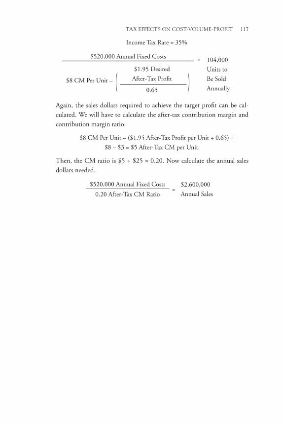
TaxeffecTsoncosT-volume-ProfiT 117
Income Tax Rate = 35%
$520,000 Annual Fixed Costs = 104,000
Units to
Be Sold
Annually$8 CM Per Unit – (
$1.95 Desired
After-Tax Profit )0.65
Again, the sales dollars required to achieve the target profit can be cal-culated. We will have to calculate the after-tax contribution margin and contribution margin ratio:
$8 CM Per Unit – ($1.95 After-Tax Profit per Unit ÷ 0.65) =
$8 – $3 = $5 After-Tax CM per Unit.
Then, the CM ratio is $5 ÷ $25 = 0.20. Now calculate the annual sales dollars needed.
$520,000 Annual Fixed Costs=
$2,600,000
Annual Sales0.20 After-Tax CM Ratio


Appendix A
Glossary
To establish a common set of terms that we use in this book, we offer the following.
Breakeven
Breakeven has traditionally been defined in at least five different ways. The five ways use different data to bring you to break even.
1. Net income equals zero. 2. Total revenue equals total costs. 3. Total revenue equals total variable costs plus total fixed costs. 4. Total contribution margin equals total fixed costs. 5. Net present value equals zero.
Business Model
A business model is your plan for your business, briefly expressed in simple terms and simple structure. It may be written in outline form or as bullet points. The concepts and calculations of breakeven and cost-volume-profit analysis (explained later), as part of your business model, show you how much work you must do to pay your costs and achieve profitability.
The business model is composed of two elements: (a) a story that describes how the enterprise works and the key assumptions that sup-port the story and (b) financial estimates that describe the way the orga-nization will add profit for investors as a result of the operations of the revenue stream and expense structure.1 The revenue stream and expense structure are built on assumptions (the story) about how the organiza-tion operates in its environment. The business model can be expressed in
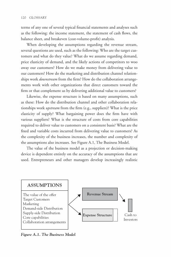
120 Glossary
terms of any one of several typical financial statements and analyses such as the following: the income statement, the statement of cash flows, the balance sheet, and breakeven (cost-volume-profit) analysis.
When developing the assumptions regarding the revenue stream, several questions are used, such as the following: Who are the target cus-tomers and what do they value? What do we assume regarding demand, price elasticity of demand, and the likely actions of competitors to woo away our customers? How do we make money from delivering value to our customers? How do the marketing and distribution channel relation-ships work downstream from the firm? How do the collaboration arrange-ments work with other organizations that direct customers toward the firm or that complement us by delivering additional value to customers?
Likewise, the expense structure is based on many assumptions, such as these: How do the distribution channel and other collaboration rela-tionships work upstream from the firm (e.g., suppliers)? What is the price elasticity of supply? What bargaining power does the firm have with various suppliers? What is the structure of costs from core capabilities required to deliver value to customers on a consistent basis? What are the fixed and variable costs incurred from delivering value to customers? As the complexity of the business increases, the number and complexity of the assumptions also increases. See Figure A.1, The Business Model.
The value of the business model as a projection or decision-making device is dependent entirely on the accuracy of the assumptions that are used. Entrepreneurs and other managers develop increasingly realistic
ASSUMPTIONS
The value of the offerTarget CustomersMarketingDemand-side DistributionSupply-side DistributionCore capabilitiesCollaboration arrangements
Revenue Stream
Expense Structure Cash toInvestors
Figure A.1. The Business Model

Glossary 121
assumptions as they gain experience. Potential investors evaluate the accuracy of the assumptions when determining whether to invest in the firm. However, judgments regarding assumptions are subject to the same biases and errors as are other managerial judgments.2 For example, unwarranted optimism is a problem for all managers. This can lead the manager to accept overly optimistic assumptions regarding the revenue stream as well as being overly optimistic regarding the ability of the firm to keep costs low.
Contribution Margin
Total revenue minus total variable costs equals total contribution mar-gin. Contribution margin per unit is calculated revenue (selling price) per unit minus variable cost per unit.
Certain types of organizations tend to exhibit certain cost behaviors. For example, universities, hospitals, and accounting and law firms tend to have a high proportion of their costs as fixed costs and a relatively small proportion of their costs as variable costs. This means that those organi-zations tend to have (and need) very high contribution margins per unit of sales.
Contribution Margin Ratio
Contribution margin per unit divided by unit selling price is the con-tribution margin ratio. Alternatively, total contribution margin divided by total revenue is the contribution margin ratio. These calculations will produce identical results. The result is usually interpreted as a percentage. For example, if the contribution margin per unit is $7 and the selling price per unit is $10, the contribution margin ratio is 70%.
Cost of Goods Sold
The cost of goods sold is the full cost to purchase or produce the goods your business offers for sale to customers.

122 Glossary
Cost-Volume-profit Analysis
Cost-volume-profit analysis is the application of the breakeven concept. It may include calculation of a breakeven point, modification to allow for profit, and visual presentation of the results on a graph.
Successfully applying the concepts and methods of cost-volume-profit analysis requires that fixed and variable costs be accurately identified and measured. Traditional accounting and financial reporting systems, designed to comply with generally accepted accounting principles, do not provide the fixed and variable cost and contribution margin information necessary for cost-volume-profit analysis.
Fixed Costs
Fixed costs may be viewed in two ways:
1. Fixed costs per unit change in inverse proportion as the quantity (volume) of units sold increases or decreases.
2. Fixed costs in total do not change as the quantity (volume) of units sold increases or decreases. Total fixed costs can change. Inflation may increase fixed costs and deflation may decrease fixed costs while the quantity of units sold remains constant. Additionally, manage-ment decisions to change technology or capacity generally change total fixed costs incurred.
Here is an illustration of fixed cost behavior. City Transit Authority calcu-lates the fuel cost of one bus for one day at $150. If 100 people ride that bus during a day, the fuel cost is $1.50 per rider ($150 ÷ 100 people). If 250 people ride the bus during a day, the fuel cost per rider drops to $.60 ($150 ÷ 250 people).
High-Low Method
The high-low method is a simple method to separate a mixed cost into its variable and fixed cost components. This method considers only the highest cost and the lowest cost incurred during the time period and dis-regards all other cost information.

Glossary 123
Least Squares Method
The least squares method (also called the linear regression method) is a
mathematical approach to separate a mixed cost into its variable and fixed
cost components. This method, in contrast to the high-low method, con-
siders all available data of costs incurred during the time period. Viewed as
a formula, this method may seem intimidating and difficult to use. In this
book, we explain how to easily apply the linear regression method using
Excel spreadsheet commands.
Mixed Costs
Mixed costs contain some variable costs and some fixed costs, presented as
a single amount. A simple example of a mixed cost is the compensation of
a salesperson who receives a fixed salary per month plus a commission (a
percentage of sales, a variable amount).
If the organization has no history or operating data for a particular
cost, an engineering analysis may be conducted to determine the types and
amounts of costs.3
When there is historical data for a particular cost, there are several
methods available to separate a mixed cost into its variable and fixed com-
ponents. We will consider two of the more commonly used methods next.
net present Value
The net present value compares the acquisition or implementation cost of
a long-life asset, project, or opportunity against the cash expected to be
received from that asset, project, or opportunity over a period of 2 or more
future years. All revenue and cost amounts are modified (discounted) using
time value of money techniques.
Relevant Range
The relevant range is the capacity a company has to produce and sell goods
and/or services without incurring additional fixed costs. A factory operat-
ing one 8-hour shift per day may have the capacity to produce 50,000 units
per year. If that factory begins operating two 8-hours shifts per day, it has

124 Glossary
the capacity to produce 100,000 units per year. Many of the factory’s oper-ating costs, which are fixed as long as the factory runs only 8 hours per day, will increase (perhaps double) when the factory begins running 16 hours per day.
Sales Mix
The sales mix is the specific product and/or services offered for sale by a business and the relative proportion of sales of each product or service line. An appliance store might have a sales mix of 70% General Electric products and 30% Whirlpool products. Alternatively, that appliance store might have a sales mix of 80% of total revenue coming from appliances sold and 20% of total revenue coming from appliance repair service.
Total Costs
Total costs include all variable costs and all fixed costs of your business. From an accounting perspective, these are the total costs. From an eco-nomic perspective, total costs include these costs as well as the more hidden opportunity cost of capital.
Total Revenue
Total revenue is the amount charged all customers for goods and/or services they purchased from your company during the period being measured (typically month, quarter, or year). This amount may alternatively be called total sales.
Traditional Breakeven Formula
Traditionally, breakeven has been expressed in one of two ways. If the desired result is the quantity of units that must be sold to achieve breakeven, the following formula is used:
Fixed Costs
= Breakeven in Units to Be Sold = BEU.Contribution Margin
per Unit

Glossary 125
If the desired result is the dollar amount of sales required to reach breakeven, the following formula is used:
Fixed Costs
= Breakeven in Dollars to Be Sold = BE$.Contribution Margin
Ratio per Unit
Unit
A unit is the item being measured. An appliance store could consider one unit of sales when one refrigerator was sold. The expression “unit” may take on different meanings. An airline might consider one unit as one ticket sold to a passenger, or it might consider one unit as one flight from point of departure to point of arrival.
Why does clearly identifying the unit of measure matter? The iden-tification of variable costs, contribution margin, and relevant range all depend on the definition of a “unit.”
Unit Selling price
The unit selling price is the price your business charges a customer per item sold.
Variable Costs
Variable costs may be viewed in two ways:
1. Variable costs per unit do not change as the quantity (volume) of units sold increases or decreases.
2. Variable costs in total change proportionally as the quantity (vol-ume) of units sold increases or decreases.
Here is an illustration of variable cost behavior. Bill mows lawns during the summer months. He typically spends $1 for fuel for his lawnmower per lawn mowed. During May, with plenty of rain and cool temperatures, the grass grew rapidly and Bill mowed 40 lawns. Consequently, he spent $40 for fuel that month. During July, when the weather was hot and dry, Bill mowed only 20 lawns and spent only $20 for fuel.
126 Glossary
The distinction between variable cost and fixed cost can be at least partially a management decision. Labor costs may be variable if workers are paid hourly and the quantity of labor hired is adjusted more or less continuously, based on need. Conversely, labor costs may be fixed if there are union contracts that guarantee both hours paid and the rate of pay or if the number of employees is relatively constant and employees are paid on salary.4
Weighted Mean
The mean is the arithmetic average of two or more values. The mean of 7 and 3 is 5. The weighted mean (also referred to as the weighted average) assigns a proportionally greater value to some items or units and a pro-portionally smaller value to others. Here is a simple retail store example:
4 People Spent $20 Each
2 People Spent $10 Each
Simple Mean of Selling Prices: ($20 + $10) ÷ 2 = $15
Weighted Mean of Sales per Customer: (4 × $20) + (2 × $10) ÷
6 customers = $16.67 (Rounded)

Appendix B
Limitations and Criticisms
The breakeven concept and the techniques of cost-volume-profit analysis are powerful business tools. Understanding them and applying them cor-rectly can be an important part of achieving success in business. How-ever, these tools, powerful as they are, have their limitations. Recognizing these limitations is essential to correctly understanding and using cost-volume-profit analysis.1 Here are the commonly recognized limitations:
• Linearity. The first limitation is that revenues and costs are assumed to be linear. That means the selling price per unit would never change and every customer would pay exactly the same price per unit. It also means that variable costs would be exactly the same for every unit. There is no provision for discounts to be received on materials purchased or fluctuating overtime premium to be paid to employees who work different quantities of extra hours.
• Relevant range. The company would always operate within the relevant range. There would never be a need to increase or decrease capacity.
• Productivity. Productivity or technological changes would not occur to change the behavior of costs from variable to fixed. Over the history of business, technology and productivity have not been static. The shift from labor-intensive to capital-intensive industry converted some formerly variable costs to fixed costs. The same change in cost behavior (away from variable to fixed) has occurred in retail and service businesses as technology has reduced or replaced human labor with bar code readers and computer software.2
• Inventory. There would be no change in the amount of inven-tory carried by the company. The quantity of units sold would

128 LimitationsandCritiCisms
always equal the quantity purchased and/or produced. For manufacturing firms, generally accepted accounting principles divide the costs of production between unsold inventory (on the balance sheet) and sold units (on the income statement). This cost allocation presents no problem for variable costs. However, it is a problem with regard to fixed production costs when the quantity of goods produced is not the same as the quantity sold. Cost-volume-profit analysis requires that all fixed costs be accumulated for use in the analysis.
• Inflation. There would be no inflation or deflation. Inflation and deflation tend to make fixed costs appear variable. When performing a cost analysis of utilities (such as water, electricity, and natural gas) or fuel (gasoline, for example), the actual units consumed may be used in lieu of the dollar cost to eliminate the effects of inflation or deflation.
• Sales mix. If the company sells more than one product or ser-vice, the sales mix would remain constant.
• Accounting information. The accounting records are adequate and appropriate to accurately identify and measure variable and fixed costs.
• Opportunity cost. The traditional accounting approach to calculating breakeven assumes that the opportunity costs of the business model are zero when multiple years are considered.
Criticisms
Criticisms of breakeven analysis’ conceptual weaknesses historically have followed its journey since its inception.
• Simplicity. The limitations of using the basic, traditional breakeven formula have been discussed by many.3 One of the early reviews of criticisms was performed by Joel Dean4 of Columbia University. He describes four limitations: (a) the difficulty of estimating costs, (b) oversimplifying the revenue function by assuming that price remains constant, (c) consider-ing the forces that influence the company as static rather than dynamic, and (d) the fact that managers adapt to changing

LimitationsandCritiCisms 129
conditions. This set of criticisms essentially focuses on the simplicity of breakeven analysis used in the presence of complex organizations and their changing environments. Here is a case where the strength of breakeven also carries a weakness. The simplicity of traditional breakeven formulas and the assump-tions on which they are based require decision makers to think in terms of single products, simple variables, static relation-ships, a single and considered relatively static period of time, and costs divided into two categories (fixed or variable). The static nature of breakeven assumptions does not reflect the real-ity that makes up a dynamic complicated market. Breakeven analysis simply takes a snapshot. Wise managers do not think in terms of single points in time with nothing changing. Rather, they think in terms of what will change given where they have been in the past and the current situation.
• Isolation. Another criticism of breakeven analysis focuses on the relative isolation that decision makers place themselves in when using breakeven analysis. Financial decisions, market-ing decisions, and operational decisions are integrated in real life, but the data needed to make these decisions are often not integrated. Each data set comes from a different place in the organization and represents just one variable. This makes the job of a decision maker difficult. For example, production data on the number of units produced over a given time frame is distinctly different from the economic data estimating market demand or price elasticity of demand. In turn, marketing data are by nature different than the financial information. In real life, changes in production volume affect pricing, which affects price elasticity of demand and also affects the cost of materials used in production. The isolation of marketing from opera-tions from finance is partly a result of organizational specializa-tion. Operational managers typically are focused on creating efficiencies in their operational departments. This special-ized focus tends to isolate them from the chief concerns that financial decision makers have or the priorities that marketing decision makers think are important.5 Although breakeven analysis formula is criticized, it is one tool to help overcome
130 LimitationsandCritiCisms
the problem of organizational complexity. The fundamental challenge of coordination never goes away even as we continue to see new generations of technology become available. Break-even analysis was developed, in part, as one way to improve coordination of effort. When marketing, operations, and finance managers of a company come together to coordinate their efforts, they all are using breakeven thinking and lan-guage though perhaps from their own specialist perspective.
One of the difficulties in developing organization-wide systemic thinking6 is the inability of leaders to overcome parochial barriers (“silos”) that separate departments. Breakeven analysis and breakeven thinking when used in cross-departmental discussions is one tool that can break down these barriers.
Managers and scholars alike have come to understand that the last frontier of sustainable competitive advantage lies in the organizational abilities that are difficult to copy.7 Central to this is consistent coordination of effort across the entire value chain of an organization as it connects with suppliers and customers. Helping managers of all key functional areas of an organization to develop their breakeven thinking abilities and then to use these abilities collectively as they coordinate their efforts with each other offers the possibil-ity that competitive advantages gained from organizational efforts also will be sustained profitably. Without the widespread use of breakeven thinking, profitable coordination of effort becomes more difficult. One might even argue that coordination of effort without the wide use of breakeven thinking in the organization can result in the coordination of unprofitability. In short, for sustainable competitive advantages truly to remain advantageous, break-even analysis must become one of the standard, frequently used tools in every department and every level of the organization from front-line workers and first-level supervisors to the directors in the boardrooms.
Criticisms of these tools result in a paradox. On one hand, it is easy to criticize the fairly simple formula for not representing complex, dynamic circumstances. On the other hand, many managers continue to use simple breakeven analysis to help them bring dynamic thinking to the business problems they face. In spite of its many limitations and criticisms, breakeven continues to be one of the best ways to focus on the relationship between cost, volume, and profitability.8

Appendix C
A Short Genealogy of Breakeven Analysis
One could argue that the thinking behind breakeven analysis has been in use for centuries if not millennia. The development of breakeven formulas and charts, like many ideas in management, appears to have emerged out of the rich history of 19th-century economics. In practice, several streams of thought contributed to the development of the break-even tools represented in this book: the applicability of cost accounting in managerial decision making and the emphasis on efficiency, a legacy of the turbulent scientific management movement, played a part in bring-ing breakeven analysis to the forefront. Out of this social context, mar-ginal analysis, the concept of the economic indifference point, and then cost-volume-profit analysis emerged.
Business leaders in decades surrounding the transition from the 19th to the 20th century were focused on ways to increase efficiency. Businesses, especially manufacturing and the railroads, were growing in size and, because of division of labor, increasing in complexity. This growth made the process of profit-oriented decision making increasingly difficult.
Products could be shipped rapidly over long distances as at no other time in history. More and more products were heading toward commodity-like price competition, which in turn squeezed profit margins, making it more crucial to get right the profit-volume decisions.
Railroads influenced the development of modern organizations and communication systems. Downward pressure on prices from buyers of transportation services influenced railroad executives to sharpen their abilities to understand the relationships between costs, volume, and profit. As railroads opened up distribution of products into new markets, larger quantities of products became available. Commodities could be

132 AShortGeneAloGyofBreAkevenAnAlySiS
shipped from the firms of Kansas and Missouri and reach the metro-politan markets of Chicago, Philadelphia, and New York within hours. A growing middle class with income to spend solidified demand for these manufactured goods. But as the volume of production increased to meet the growing demand, the profitability of these companies changed. The speed of decision making increased to match the increased speed in dis-tribution and communication. Managers needed better tools to under-stand the impact of changing cost and revenue structures on the ability of the firm to generate a profit. In 1887 railroad engineer A. M. Wel-lington discussed how high fixed costs placed railroads at risk if they lost business. However, Wellington did not produce a breakeven formula to illustrate his point.
Differences in perspective between a company’s engineers and its business managers were starting to be recognized as barriers to further developments in the ability to be profitable.1 In spite of Frederick Tay-lor’s attempts to bridge the gap between management and labor with a scientific approach to management, the age-old conflicts between the two groups were increasing in their intensity, with both sides becoming more sophisticated in how they understood business.
Management and management engineers needed better tools for deci-sion making and for communication with each other.2 Managers started using breakeven charts.
One of the earliest focused studies of the topic in the United States came from the work of Henry Hess.3 In 1904 an article by John Mann appeared in the Encyclopedia of Accounting showing the methods for preparing breakeven charts.4 As principles of cost accounting began to mature in the 1920s, the concepts of fixed costs and variable costs came to have wider applications than in just financial accounting.5 It was the scientific management movement that brought together these developing streams of thought, which resulted in the creation of the simple break-even formula we know today. Thus, in 1922 John Williams published an article in the Bulletin of the Taylor Society that described the mathematical formula for breakeven.6
Organizational problems began to arise from increased size and com-plexity. A few years later J. O. McKinsey7 proposed that breakeven charts be used in discussions between sales, production, and finance decision makers. McKinsey’s recommendation, largely forgotten today, is that

AShortGeneAloGyofBreAkevenAnAlySiS 133
breakeven analysis should be conducted periodically for each operating unit of a company. The reason for this is that operating unit fixed costs and variable costs will vary from unit to unit. They can change with other changes taking place in the business or in the firm’s larger environment. Because of this, the sales volume necessary to generate return on invested capital also will vary by unit. At the end of each period, unit managers from sales, operations, and finance would come together to discuss their current situation and what they expected for the near-term future. Such discussions are designed to coordinate divergent areas of emphasis and integrate divergent ways of thinking.
Breakeven analysis provided an important connecting link between the assumptions that managers had about their business, the external environment, and actual business activities. It became and remains one of the more popular managerial accounting tools.
Since its introduction decades ago, the breakeven concept has been enhanced, adjusted, and extended in an attempt to reduce or correct for its limitations and make it applicable to more and more business situ-ations. During the 1940s, 1950s, and 1960s, accounting scholars and practitioners8 published articles reviewing various facets of breakeven and its use. Periodically after these three decades practicing managers and scholars made additional contributions to the subject. For example, Martin9 showed how to relate breakeven point from one year to another while taking into consideration the cost of capital, and Creese10 explored breakeven when the production quantity is fixed but the time period changes. Scholars proposed more precise and sophisticated approaches to breakeven analysis, using statistical tools when conditions are uncertain.11
Gardner, Tse, and then a generation later, Schweitzer, Trossmann, and Lawson became the first to offer book-length treatments of the topic.12 The last of these three emphasized the academic, theoretical dimensions of the concept. For many users of breakeven methods, these three books have been forgotten, though the wisdom they contain is as relevant today as when they were written.
Before and after these books many articles have been published dem-onstrating specific, practical applications of breakeven analysis or evaluat-ing its limitations as a management decision-making tool. Some scholars experimented with various ways to extend the basic concepts, while oth-ers clarified the limitations of breakeven.

134 AShortGeneAloGyofBreAkevenAnAlySiS
Breakeven analysis has become a traditional component of introduc-tory accounting, marketing, management, and entrepreneurship text-books. A common feature of these texts is that, probably due to space limitations, such books typically present just one or two of the most basic methods to teach the concept. More advanced managerial accounting, managerial economics, and business finance texts also include short sec-tions on breakeven. By the time undergraduate students arrive at their senior capstone course, they are expected to understand breakeven analy-sis when analyzing cases. Sadly, the few applications found in introduc-tory textbooks do not adequately prepare students to determine whether the firms they study are breaking even.
What has been lacking for several years is a product that collects and explores the practical applications of breakeven thinking useful to a variety of industries and decision situations, but that is not so academic as to put off many busy practicing managers. We present in this book the applica-tions and approaches we believe most managers will find useful, leaving the more complicated methods to explore another day. Thus, this book is not intended to be a comprehensive encyclopedia of breakeven methods but rather a practical analytic tool belt that practicing managers and students can relatively quickly add to their business decision-making skills.
The activity of calculating the breakeven point is necessary for just about every organization in existence. It is difficult to think of even one example where the entrepreneurs and the venture capitalists or angel investors of start-up companies would not be interested in knowing the breakeven point for their venture. Likewise, corporate entrepreneurs starting new profit centers use breakeven thinking. Years ago, when man-ufacturing firms were focusing on making a profit producing and selling one or two products, the basic formula worked well. But life has changed. Service businesses now dominate the market landscape. Now breakeven analysis is employed to help decision makers solve problems that encom-pass the context of the entire value chain of the firm at the same time as solving specific operational problems.

Appendix d
Using Breakeven Thinking to decide Whether to Start a Business
Breakeven thinking begins before you start a business. For example, start-ing your own golf course and pro-shop business requires that you com-pare what you could gain from your work in the corporate world with the prospects of owning and operating your own business. You will compare both tangible and intangible dimensions.
Of all the factors that influence your decision of whether to go into business, the financial questions can be some of the most challenging. Some financial elements are less certain, especially at the beginning. And yet, when you are about to start a business, you have to take this uncer-tainty and somehow make your best guess as to how it will work out.
Applied to the decision of whether to quit your job and start a busi-ness, breakeven thinking becomes a comparison between what you could earn either way over a defined period of time.
The Formula
The breakeven formula used for this decision is a gross estimate based on many assumptions about market demand, the presence and actions of competitors in the market, the revenue stream of the business, the expense structure of the business, and all the assumptions related to keep-ing one’s job. The formula is
BE = (R – [CA + CO]) + DV = 0,
where
136 UsingBreakevenThinking
BE = Breakeven Point
R = Revenue Expected From Starting the Company
CA = Accounting Costs Expected to Be Incurred by
Operating the Company
CO = Opportunity Costs Expected to Be Incurred by
Quitting Your Job
DV = Change in the Total Value of the Firm as a
Result of Starting and Operating the Business.
If the result is a positive number (above the breakeven point of zero),
then financially the decision makes sense. If the result is a negative num-
ber, then financially at least the decision would be unwise.
You will notice that two types of costs are included in this formula:
accounting costs and opportunity costs. Accounting costs are the more
familiar term. They will show up in the income statement. You can think
of these as the operating expenses to run the company or the costs you
incur to generate operating revenue. Opportunity costs are different.
These are the economic costs from giving up what you might have earned
by taking your next best alternative. In the case of deciding whether to
quit your job and start a business, one opportunity cost is the after-tax
wages and benefits you could have earned over a defined period of time
by staying with your current job and not starting a business. These wages
and benefits you will have to give up if you start a full-time business.
Other opportunity costs include what you could earn from putting (or
keeping) your cash in an investment other than starting a business—such
as a money market account or your personal property. You incur these
costs when you start a business and take your personal assets such as cash
or give up your wage-earning job. These costs do not show up in the
income statement, but they are (economic) costs.
Example
Consider Tally Richey, a 35-year-old woman, her husband Donovan, and
their two young children. They live on 150 acres of land that contains
three ponds and two running streams. Their business idea is to develop
just half of the property into a golf course (nine holes) and small pro
shop. The business would be a sole proprietorship. They plan to expand
UsingBreakevenThinking 137
it to a full 18 holes a few years later as they build customer support and
generate cash for landscape construction. They even have dreams of even-
tually buying the neighbor’s property of 200 acres. Right now they have
$100,000 of equity in their property, which they could refinance. Of
this, $50,000 now sits in the family money market account that earns
an annual percentage rate of 6%. They will have access to this cash when
the money market instrument matures in 6 months. They plan to use
this $50,000 to construct the landscape for the bare minimum needed to
open the first nine holes. This will include one large putting green, nine
tees, fairways and greens, and a driving range. They will also purchase two
pieces of equipment for mowing—one for fairways and one for greens.
Let’s assume that since the business requires their full-time commitment,
they will have to quit their jobs. In the business they will employ a few
part-time workers.
Neither Tally nor Donovan has direct experience actually operating
a public golf course. They have been avid golfers for 5 years and love
the sport. They have a close circle of golfing-enthusiast friends, some of
whom have spoken about the natural beauty of the Richey property and
what a great golf course it could make. Clearly it is the asset of land and
their passion for golf that might give Tally and Donovan a good start for
their business idea.
Curious about whether the business would generate a profit, Tally asks
a friend who is an accountant to prepare a projected income statement for
the first 3 years of business operations. This they turn into a breakeven
study, comparing their projections with what they could achieve by keep-
ing their jobs.
Based on the information that Tally and Donovan gave the accoun-
tant, he brings them information given in Table D.1, Projected Breakeven
Statement.
Sales projections are based on Tally and Donovan’s estimates for the
number of golfing customers paying a fixed amount for greens fees and
other products. To begin with, the company will sell just a few items,
such as a single line of golf clubs, putters, tees, and golf balls. Accounting
costs include the costs of maintaining the nine-hole golf course, operat-
ing the tiny pro shop, and marketing. Tally and Donovan will pay them-
selves a wage for some of these expenses and can choose to take the rest

138 UsingBreakevenThinking
as a bonus at the end of the time period, or take the rest and invest it in growing the business.
Of course there are other options to consider for starting the business, which would make the financial projection results come out differently. For example, Tally could keep her job and Donovan could quit his job to oversee the landscape construction and opening of the business. Tally’s job could provide the family with personal cash flow so they can keep making payments on their mortgage and living expenses. Assuming for sake of discussion that Tally and Donovan each earn roughly the same amount, Table D.2 presents a revised projected breakeven statement.
Summary
This type of breakeven study is a big-picture analysis. If Tally and Dono-van can keep the business growing for 3 years and meet their assumptions, starting this business might be worth it. But this is a big IF! Nothing is guaranteed. Their assumptions about market demand, revenue, and expense structure may be unrealistic if they lack experience working at a golf course.
Table D.1. Projected Breakeven Statement
Year 1 Year 2 Year 3 3-year totalsales $350,000 $500,000 $750,000 $1,600,000
Lesscostofgoodssold $60,000 $80,000 $120,000 $260,000
grossprofit $290,000 $420,000 $630,000 $1,340,000
Lessaccountingcosts(operatingexpenses)
$210,000 $310,000 $470,000 $990,000
netprofit(beforeincometaxes)
$80,000 $110,000 $160,000 $350,000
Lessopportunitycosts* ($166,000) ($172,000) $178,000) ($516,000)
Dvestimatedchangeinthevalueofthefirm**
$50,000 $50,000 $75,000 $155,000
above(Below)breakeven ($36,000) ($12,000) $57,000 $9,000
*Both Tally and Donovan giving up 3 years of salary and benefits plus the opportunity to invest $50,000 from the money market account, which now earns 6% interest.
**Considering the change in total value of the business (including the value of the developed property and what the business might be sold for at the end of the time period).

UsingBreakevenThinking 139
This application of breakeven analysis is not foolproof. Projecting the financial impact of one business idea compared with its best alternative (keeping your job) requires them to make their best reasonable estimates. Enthusiasm over an interesting business idea can cloud their judgment. Because financial projections are estimates based on assumptions that they make, Tally and Donovan may be tempted to do some interesting things with their estimates. For example, they may be tempted to under-represent opportunity costs. They may be aggressive with their assump-tions regarding market demand, pricing, and sales. Or they may be less realistic regarding projected operating expenses.
Table D.2. Revised Projected Breakeven Statement
Year 1 Year 2 Year 3 3-year totalsales $350,000 $500,000 $750,000 $1,600,000
Lesscostofgoodssold $60,000 $80,000 $120,000 $260,000
grossprofit $290,000 $420,000 $630,000 $1,340,000
Lessaccountingcosts(operatingexpenses)
$210,000 $310,000 $470,000 $990,000
netprofit(beforeincometaxes)
$80,000 $110,000 $160,000 $350,000
Lessopportunitycosts* ($86,000) ($92,000) ($95,000) ($516,000)
Dvestimatedchangeinthevalueofthefirm**
$50,000 $0,000 $75,000 $155,000
above(Below)breakeven $44,000 $68,000 $140,000 $252,000
*Donovan only giving up 3 years of salary and benefits plus the opportunity to invest $50,000 from the money market account, which now earns 6% interest.
**Considering the change in total value of the business (including the value of the developed property and what the business might be sold for at the end of the time period).


Appendix e
Annuity TableYears 4% 5% 6% 7% 8% 9% 10% 11%
1 0.962 0.952 0.943 0.935 0.926 0.917 0.909 0.901
2 1.886 1.859 1.833 1.808 1.783 1.759 1.736 1.713
3 2.775 2.723 2.673 2.624 2.577 2.531 2.487 2.444
4 3.630 3.546 3.465 3.387 3.312 3.240 3.170 3.102
5 4.452 4.329 4.212 4.100 3.993 3.890 3.791 3.696
6 5.242 5.076 4.917 4.767 4.623 4.486 4.355 4.231
7 6.002 5.786 5.582 5.389 5.206 5.033 4.868 4.712
8 6.733 6.463 6.210 5.971 5.747 5.535 5.335 5.146
9 7.435 7.108 6.802 6.515 6.247 5.995 5.759 5.537
10 8.111 7.722 7.360 7.024 6.710 6.418 6.145 5.889
11 8.760 8.306 7.887 7.499 7.139 6.805 6.495 6.207
12 9.385 8.863 8.384 7.943 7.536 7.161 6.814 6.492
13 9.986 9.394 8.853 8.358 7.904 7.487 7.103 6.750
14 10.563 9.899 9.295 8.745 8.244 7.786 7.367 6.982
15 11.118 10.380 9.712 9.108 8.559 8.061 7.606 7.191
discount rate per yearYears 12% 13% 14% 15% 16% 17% 18% 19% 20%
1 0.893 0.885 0.877 0.870 0.862 0.855 0.847 0.840 0.833
2 1.690 1.668 1.647 1.626 1.605 1.585 1.566 1.547 1.528
3 2.402 2.361 2.322 2.283 2.246 2.210 2.174 2.140 2.106
4 3.037 2.974 2.914 2.855 2.798 2.743 2.690 2.639 2.589
5 3.605 3.517 3.433 3.352 3.274 3.199 3.127 3.058 2.991
6 4.111 3.998 3.889 3.784 3.685 3.589 3.498 3.410 3.326
7 4.564 4.423 4.288 4.160 4.039 3.922 3.812 3.706 3.605
8 4.968 4.799 4.639 4.487 4.344 4.207 4.078 3.954 3.837
9 5.328 5.132 4.946 4.772 4.607 4.451 4.303 4.163 4.031
10 5.650 5.426 5.216 5.019 4.833 4.659 4.494 4.339 4.192
11 5.938 5.687 5.453 5.234 5.029 4.836 4.656 4.486 4.327
12 6.194 5.918 5.660 5.421 5.197 4.988 4.793 4.611 4.439
13 6.424 6.122 5.842 5.583 5.342 5.118 4.910 4.715 4.533
14 6.628 6.302 6.002 5.724 5.468 5.229 5.008 4.802 4.611
15 6.811 6.462 6.142 5.847 5.575 5.324 5.092 4.876 4.675


Notes
Chapter 1
1. Bell (1969); Dean (1948); Earley (1955); Kempster (1949); Soldofsky(1959);Weiser(1969).
Chapter 2
1.Weygandt,Kimmel,andKieso(2009). 2.Kempster(1949).
Chapter 4
1.Bell(1969),p.34.
Chapter 5
1.Mariotti(2007). 2.SeeGardner(1955). 3.KimesandThompson(2004).
Chapter 6
1.Kurtz(2008). 2.PindyckandRubinfeld(2001). 3.PindyckandRubinfeld(2001). 4.Mansfield,Allen,Doherty,andWeigelt(2002). 5.Mansfield,Allen,Doherty,andWeigelt(2002). 6.Mansfield,Allen,Doherty,andWeigelt(2002). 7.Kurtz(2008). 8.SmithandNagle(1994).
Chapter 7
1.Hilton(2009),p.290.

144 Notes
Chapter 8
1.Hilton(2009),p.247.
Chapter 9
1.Hilton(2009),pp.256–257. 2.Garrison,Noreen,andBrewer(2008),p.203. 3.HansenandMowen(2007),p.87. 4.HansenandMowen(2007),p.87.
Chapter 10
1.SmithandNagle(1994). 2.Tse(1960).
Chapter 11
1.SmithandNagle(1994). 2.Tse(1960),p.81.
Chapter 12
1.HansenandMowen(2007),pp.536–537.
Chapter 14
1.ForadditionalinformationonMACRSdepreciation,thereaderisdirectedtoHilton(2009),pp.698–700. 2.Forinformationonincorporatinginflationintotheanalysis,thereaderisdirectedtoHilton(2009),pp.718–720. 3.Brealey,Myers,andMarcus(2008). 4.Guidry,Horrigan,andCraycraft(1998). 5.BrealeyandMyers(2000). 6.Kempster(1949);Soldofsky(1959). 7.Cheung&Heaney(1990);FreemanandFreeman(1993);Guidry,Hor-rigan,andCraycraft(1998);Kee(2007). 8.KinneyandRaiborn(2008). 9.BrealeyandMyers(2000),p.27.

Notes 145
Chapter 15
1.PresentedinBarnettandZiegler(1991). 2.BarnettandZiegler(1991). 3.BattistaandCrowningshield(1966),pp.14–15. 4. Brandenburger and Nalebuff (1996); Pindyck and Rubinfeld (2001),p.23;Porter(1980),p.167.
Chapter 16
1.Hilton(2009),pp.304–306.
Appendix A
1.Magretta(2002);Schweizer(2005). 2.Bazerman(2006). 3.Garrison,Noreen,andBrewer(2008),pp.201–202. 4.Garrison,Noreen,andBrewer(2008),p.197.
Appendix B
1. Anderson (1957); Bell (1969); Chung (1993); Conway (1957); Fearon(1960);FreemanandFreeman(1993);Kee(2007);Schweitzer,Trossmann,andLawson(1992);Soldofsky(1959);Weiser(1969);Yacobian(1959). 2.Garrison,Noreen,andBrewer(2008),p.196. 3. Including Battista and Crowningshield (1966); Conway (1957); Dean(1948); Johnson (1965);Kempster (1949);Klipper (1978); Soldofsky (1959);Warthen(1972);andYacobian(1959). 4.Dean(1948). 5.Schein(1996). 6.Senge(1990). 7.Child(2005);Maital(1994);Porter(1996);PrahaladandHamel(1990). 8.Kempster(1949);Weiser(1969);Yacobian(1959).
Appendix C
1.Galbraith(1987),p.172;Veblen(1904). 2.ComparewithKempster(1949),p.712. 3.Hess(1897);Hess(1903). 4.NationalAssociationofCostAccountants(1949). 5.Earley(1955).

146 Notes
6.Chatfield(1974). 7.McKinsey(1924). 8.SuchasDean(1948);Earley(1955);Kempster(1949);Tuttle(1959);andWeiner(1960). 9.Martin(1985). 10.Creese(1993). 11.FinchandGavirneni(2006);Yunker(2001);Yunker(2006). 12.Gardner(1955);Schweitzer,Trossmann,andLawson(1992);Tse(1960).

References
Anderson, C. W. (1957). Disclosure of assumptions key to better break-even analysis. National Association of Accountants NAA Bulletin, 39(4), 25–30.
Barnett, R. A., & Ziegler, M. R. (1991). Essentials of college mathematics: For business, economics, life sciences and social sciences (2nd ed.). New York: Dellen.
Battista, G. L., & Crowningshield, G. R. (1966). Cost behavior and breakeven analysis—a different approach. National Association of Accountants NAA Man-agement Accounting, 48(2), 3–16.
Bazerman, M. H. (2006). Judgment in managerial decision making (6th ed.). New York: John Wiley & Sons.
Bell, A. L. (1969). Break-even charts versus marginal graphs. Management Accounting, 59(6), 32–35, 48.
Brandenburger, A. M., & Nalebuff, B. J. (1996). Co-opetition. New York: Doubleday.
Brealey, R. A., & Myers, S. C. (2000). Principles of corporate finance (6th ed.). Boston: Irwin McGraw-Hill.
Brealey, R. A., Myers, S. C., & Marcus, A. J. (2008). Fundamentals of corporate finance (6th ed.). New York: McGraw-Hill.
Chatfield, M. (1974). A history of accounting thought. Hinsdale, IL: The Dryden Press.
Cheung, J. K., & Heaney, J. (1990). A contingent-claim integration cost- volume-profit analysis with capital budgeting. Contemporary Accounting Research, 6(2), 738–760.
Child, J. (2005). Organization: Contemporary principles and practice. Malden, MA: Blackwell.
Chung, K. H. (1993). Cost-volume-profit analysis under uncertainty when the firm has production flexibility. Journal of Business Finance & Accounting, 20(4), 583–592.
Conway, R. W. (1957). Breaking out of the limitations of break-even analysis. National Association of Cost Accountants NACA Bulletin, 38(10), 1265–1272.
Creese, R. C. (1993). Break-even analysis—The fixed quantity approach. Trans-actions of AACE International, A.1, pp. A.1.1.–A.1.7.
Dean, J. (1948). Cost structures of enterprises and break-even charts. The Ameri-can Economic Review. Papers and Proceedings of the Sixtieth Annual Meeting of the American Economic Association, 38(2), 153–164.

148 RefeRences
Earley, J. S. (1955). Recent developments in cost accounting and the “marginal analysis.” Journal of Political Economy, 63(3), 227–242.
Fearon, H. E. (1960). Constant product mix a limiting assumption in B-E analy-sis. National Association of Accountants NAA Bulletin, 41(11), 61–67.
Finch, B., & Gavirneni, S. (2006). Confidence intervals for optimal selection among alternatives with stochastic variable costs. International Journal of Pro-duction Research, 44(20), 4329–4342.
Freeman, M., & Freeman, K. (1993). Considering the time value of money in breakeven analysis. Management Accounting, 71(1), 50–52.
Galbraith, J. K. (1987). A history of economics. London: Penguin Books.Gardner, F. V. (1955). Profit management and control. New York: McGraw-Hill.Garrison, R. H., Noreen, E. W., & Brewer, P. C. (2008). Managerial accounting
(12th ed.). New York: McGraw-Hill Irwin.Guidry, F., Horrigan, J. O., & Craycraft, C. (1998). CVP analysis: A new look.
Journal of Managerial Issues, 10(1), 74–85.Hansen, D. R., & Mowen, M. M. (2007). Managerial accounting (8th ed.).
Mason, OH: Thomson South-Western.Hess, H. (1897). Time saving and its relation to profits. Engineering Magazine,
20, 935 ff.Hess, H. (1903). Manufacturing: Capital, costs, profits, and dividends. Engineer-
ing Magazine, 24, 367 ff.Hilton, R. W. (2009). Managerial accounting: Creating value in a dynamic business
environment (8th ed.). New York: McGraw-Hill Irwin.Johnson, C. H. (1965). B-E analysis in cost control. National Association of
Accountants NAA Bulletin, 46(8), 64.Kee, R. (2007). Cost-volume-profit analysis incorporating the cost of capital.
Journal of Managerial Issues, 19(4), 478–493.Kempster, J. H. (1949). Break-even analysis—common ground for the econo-
mist and the cost accountant. National Association of Cost Accountants NACA Bulletin, 39(12), 711–720.
Kimes, S. E., & Thompson, G. M. (2004). Restaurant revenue management at Chevys: Determining the best table mix. Decision Sciences, 35(3), 371–392.
Kinney, M. R., & Raiborn, C. A. (2008). Cost accounting: Foundations and evolu-tions (7th ed.). Mason, OH: Cengage Learning.
Klipper, H. (1978). Breakeven analysis with variable product mix. Management Accounting, 59(10), 51–54.
Kurtz, D. L. (2008). Contemporary marketing (13th ed.). Mason, OH: Thomson South-Western.
Magretta, J. (2002). Why business models matter. Harvard Business Review, 85(5), 86–92.
Maital, S. (1994). Executive economics. New York: The Free Press.

RefeRences 149
Mansfield, E., Allen, W. B., Doherty, N. A., & Weigelt, K. (2002). Managerial economics: Theory, applications, and cases (5th ed.). New York: W. W. Norton.
Mariotti, S. (2007). Entrepreneurship: Starting and operating a small business. Upper Saddle River, NJ: Pearson Prentice Hall.
Martin, H. (1985). Breaking through the breakeven barriers. Management Accounting, 66(11), 31–34.
McKinsey, J. O. (1924). Co-ordination of sales, production, and finance. The University Journal of Business, 2(4), 399–405.
National Association of Cost Accountants. (1949). The analysis of cost-volume-
profit relationships. National Association of Cost Accountants NACA Bulletin,
31(4), 523–564.
Pindyck, R. S., & Rubinfeld, D. L. (2001). Microeconomics (5th ed.). Upper
Saddle River, NJ: Prentice Hall.
Porter, M. E. (1980). Competitive strategy: Techniques for analyzing industries and
competitors. New York: The Free Press.
Porter, M. E. (1996). What is strategy? Harvard Business Review, 74(6), 61–78.
Prahalad, C. K., & Hamel, G. (1990). The core competence of the corporation.
Harvard Business Review, 68(3), 79–91.
Schein, E. H. (1996). Three cultures of management: The key to organizational
learning. Sloan Management Review, 38(1), 9–20.
Schweitzer, M., Trossmann, E., & Lawson, G. H. (1992). Break-even analyses: Basic model, variants, extensions. New York: John Wiley & Sons.
Schweizer, L. (2005). Concept and evolution of business models. Journal of Gen-eral Management, 31(2), 37–56.
Senge, P. (1990). The fifth discipline. New York: Doubleday.
Smith, G. E., & Nagle, T. T. (1994). Financial analysis for profit-driven pricing.
Sloan Management Review, 35(3), 71–84.
Soldofsky, R. M. (1959). Accountant’s vs. economist’s concepts of break-even
analysis. National Association of Cost Accountants NACA Bulletin, 41(4),
5–18.
Tse, J. Y. D. (1960). Profit planning through volume-cost analysis. New York:
Macmillan.
Tuttle, R. E. (1959). The effect of inventory change on break-even analysis.
National Association of Accountants NAA Bulletin, 40(5), 77–87.
Veblen, T. (1904). The theory of business enterprise. New York: Charles Scribner’s
Sons.
Warthen, W. H. F., Jr. (1972). Mix variances in profit rate analysis. Management Accounting, 53(12), 43–45.
Weiner, J. (1960). To better results through a more accurate break-even formula.
National Association of Cost Accountants NACA Bulletin, 41(11), 5–18.

150 RefeRences
Weiser, H. J. (1969). Break-even analysis: A re-evaluation. Management Account-ing, 50(6), 36–41.
Weygandt, J. J., Kimmel, P. D., & Kieso, D. E. (2009). Accounting principles (9th
ed.). New York: John Wiley & Sons.
Yacobian, P. (1959). A practical evaluation of breakeven analysis. National Asso-ciation of Accountants NAA Bulletin, 40(5), 23–29.
Yunker, J. A. (2001). Stochastic CVP analysis with economic demand and cost
functions. Review of Quantitative Finance and Accounting, 17(2), 127–149.
Yunker, J. A. (2006). Incorporating stochastic demand into breakeven analysis: A
practical guide. Engineering Economist, 51(2), 161–193.
Further Reading
Baber, W. R., Ijiri, Y., & Kang, S. H. (1996). Profit-volume-exchange-rate analy-
sis for planning international operations. Journal of International Financial Management and Accounting, 7(2), 85–101.
Bozarth, C. C., & Handfield, R. B. (2006). Introduction to operations and supply chain management. Upper Saddle River, NJ: Pearson Prentice Hall.
Bracken, R. M., & Volkan, A. G. (1988). Cash flow disclosures & break-even
analysis. The National Public Accountant, 33(6), 48–51.
Conine, T. E., Jr. (1987). A pedagogical note on cash break-even analysis. Journal of Business Finance & Accounting, 14(3), 437–441.
Coppage, R. E., & Blum, L. M. (2007). Breakeven point analysis aids in evaluat-
ing ROTH conversions. Practical Tax Strategies, 78(2), 83–89.
Eckholdt, J. L. (1960). Using the break even chart in product-line decisions.
National Association of Accountants NAA Bulletin, 41(11), 43–50.
Gapenski, L. C. (1989). Analysis provides test for profitability of new services.
Healthcare Financial Management, 43(11), 48–58.
Gitman, L. J. (2000). Principles of managerial finance. Reading, MA:
Addison-Wesley.
Harris, P. (1999). Profit planning (Hospitality Industry). (2nd ed.). Woburn,
MA: Butterworth-Heinemann.
Heizer, J., & Render, B. (2001). Operations management (6th ed.). Upper Saddle
River, NJ: Prentice Hall.
Kaplan, R. S., & Atkinson, A. A. (1989). Advanced management accounting (2nd
ed.). Englewood Cliffs, NJ: Prentice Hall.
Kuratko, d. f., & Hodgetts, R. M. (2004). Entrepreneurship: Theory, process, prac-tice (6th ed.). Mason, OH: Thomson South-Western.
Larimore, L. K. (1974). Break-even analysis for higher education. Management Accounting, 56(3), 25–28.

RefeRences 151
O’Neil, C. J., & Shackelford, D. A. (1989). An automobile lease-buy decision model. Journal of Accountancy, 168(3), 154–162.
Razek, J. R. (1989). Gain control of your organization’s finances: Break-even analysis. Nonprofit World, 7(5), 30–33.
Render, B., & Stair, R. M., Jr. (1997). Quantitative analysis for management (6th ed.). Upper Saddle River, NJ: Prentice Hall.
Rigsbee, S. R., Ayaydin, S. S., & Richard, C. A. (1992). Secondary marketing: Pricing for profits. Mortgage Banking, 52(5), 65–71.
Sherman, L. F., Shim, J. K., & Hartney, M. (1993). Short run break-even analy-sis for real estate projects. Real Estate Issues, 18(1), 15–20.
Shim, J. K., & Constas, M. (1997). Does your nonprofit break even? The CPA Journal, 67(12), 36–42.
Suver, J. D., & Neumann, B. R. (1977). Patient mix and breakeven analysis. Management Accounting, 58(7), 38–40.
Willson, J. D. (1960). Practical applications of cost-volume-profit analysis. National Association of Accountants NAA Bulletin, 41(7), 5–19.


Index
Aaccounting information, 128activity and cost data, high-low
method, 55talgebraic format of PowerRoll data, 97tannuity table, 141
BBarnett, R. A., 108Bell, A. L., 19benefits
cost of goods sold (COGS) method, 25–27
product mix, 43–44breakeven analysis
about, 1and business situations, 2–3and cost of capital, 95defined, 119genealogy, 131–34starting business and, 135–39traditional formula, 2See also modified breakeven analysis
breakeven income statement, 12tbreakeven points at different price
levels, 36tBrealey, R. A., 95Bulletin of the Taylor Society, 132business model, 119–21, 120fbusiness situations, breakeven analysis
and, 2–3
Ccalculating
coefficient of determination, 59f
fixed delivery cost, 58fvariable delivery cost, 58f
capital asset pricing model (CAPM), 98
changingcosts, 65–74fixed costs, 69–74, 70tprices, 75–83in product mix, 41–49revenue and costs, quadratic equa-
tion, 109tvariable costs, 67–69, 69t
comparisonbreakeven methods, 98tbreakeven points, quadratic equa-
tion, 110fto high-low, least squares method,
60tconstant profit curve, modified break-
even analysis, 37fcontribution margin (CM), 11–16,
121with cost inflation, 65tdecreasing, fixed costs increasing,
73tincreasing, fixed costs increasing,
72twith new selling price, 66tresults interpretation, 12–13
contribution margin ratio (CM ratio), 13–15
defined, 121operating leverage, 15–16
cost inflation, 65t
Note: The f and t following page numbers refers to figures and tables, respectively.

154 Index
cost of goods sold (COGS), 21–28, 121
benefits, 25–27formula, 21limitations, 27–28results interpretation, 22–25
costs and revenue changing, quadratic equation, 108–10
cost-volume-profit analysis, 1defined, 122tax effects on, 115–17
Creese, R. C., 133criticisms, 128–30customer responsiveness, modified
breakeven analysis, 31–33
DDean, Joel, 128deliveries and costs, least squares
method, 57tdemand
estimated, 31–33, 32t–33tfactoring estimates, 29–39and modified breakeven analysis,
29–31factoring in modified breakeven
analysis, 34–35schedule, 34f
Eelastic demand curve, modified break-
even analysis, 38, 38fEncyclopedia of Accounting, 132estimating demand methods, 31–33,
32t–33tethics
modified breakeven analysis, 39net present value (NPV) method,
102–3
Ffactoring demand
estimates, 29–39in modified breakeven analysis,
34–35fixed costs (FC), 6, 122
calculation, 54tchanging, 69–74, 70t
contribution margin decreasing, 73tcontribution margin increasing, 72t
fixed desired profit, 17formulas
cost of goods sold (COGS), 21extending, 9–10product mix, 41–42, 44–45starting business, 135–38total cost method, 7
GGardner, F. V., 133genealogy, breakeven analysis, 131–34generally accepted accounting prin-
ciples (GAAP), 23
HHess, Henry, 132high-low method, 51–56
activity and cost data, 55tdefined, 122example, 52tfixed cost calculation, 54tmaintenance costs versus miles
driven, 53tnatural gas use, 53toutlier example, 52t
Iindifference points, 93, 131
net present value (NPV) method, 94t
inelastic demand curve, modified breakeven analysis, 37f
inflation, 128inventory, 127–28isolation, 129
KKurtz, D. L., 34
LLawson, G. H., 133least squares method, 57–63
calculating coefficient of determina-tion, 59f
calculating fixed delivery cost, 58f

Index 155
calculating variable delivery cost, 58f
compared to high-low method, 60tdefined, 123deliveries and costs, 57tscattergraph, 61, 62f–63f
limitations, 127–28cost of goods sold (COGS)
method, 27–28product mix, 48–49quadratic equation, 111–13
linear cost curve, quadratic equation, 108f
linearity, 127
Mmaintenance costs versus miles
driven, high-low method, 53tMann, John, 132Marcus, A. J., 95Martin, H., 133McKinsey, J. O., 132mixed costs, 123modified breakeven analysis, 29–39
alternatives, 35–38breakeven points at different price
levels, 36tconstant profit curve at various
prices, 37fcustomer responsiveness, 31–33demand, 29–31demand schedule, 34felastic demand curve, 38, 38festimating demand methods,
31–33, 32t–33tethical dimension, 39factoring demand in, 34–35factoring estimates of demand,
29–39inelastic demand curve, 37foptimal profit graph, 35fprice-demand relationship, 30fSee also breakeven analysis
multiple breakeven points, 89–91multiple regression, 61Myers, S. C., 95
NNagle, T. T., 35, 38, 67, 75natural gas use, high-low method,
53tnet income at economic breakeven,
98tnet present value (NPV), 93–103
algebraic format of PowerRoll data, 97t
breakeven and cost of capital, 95comparison of breakeven methods,
98tdefined, 123ethical considerations, 102–3indifference point calculation
steps, 94tnet income at economic break-
even, 98tobservations, 99PowerRoll data, 96tsensitivity analysis, 101tstatewide industries data, 94tvariations, 99–100weaknesses, 100–102
new selling price, contribution mar-gin (CM) with, 66t
nonlinear cost and revenue curves, quadratic equation, 109f
Oobservations, net present value
(NPV) method, 99operating leverage, contribution mar-
gin ratio (CM ratio), 15–16opportunity cost, 128optimal profit graph, modified break-
even analysis, 35foutlier example, high-low method,
52toutsource decision, 93
Pprice-demand relationship, modified
breakeven analysis, 30fprices
changing, 75–83elasticity of demand, 31
productivity, 127

156 Index
product mixbenefits, 43–44, 48dealing with changes in, 41–49formulas, 41–42, 44–45
product mix (cont.)limitations, 48–49results interpretation, 47–48sales mix, 42t–43tweighted average selling price
method, 44profitability, 130projected breakeven statement, start-
ing business, 138t–39t
Qquadratic equation, 105–13
changes in revenue, 106–8changing revenue and costs, 109tcomparison of breakeven points,
110fcosts and revenue changing,
108–10limitations, 111–13linear cost curve, 108fnonlinear cost and revenue curves,
109frevenue and costs, 106t
Rrailroads, 131relevant range, 127
defined, 123–24results interpretation, 7–8
contribution margin method, 12–13
cost of goods sold (COGS) method, 22–25
product mix, 47–48revenue, quadratic equation, 106–8,
106t
Ssales mix, 128
defined, 124product mix, 42t–43t
scattergraphs, least squares method, 61, 62f–63f
Schweitzer, M., 133
selling price (SP), 36simple average, 45, 45tat various volumes, 85–87weighted average, 45, 45t
sensitivity analysis, net present value (NPV), 101t
simple average selling price (SP), 45, 45t
simplicity, 128–29simplified income statement, 22tSmith, G. E., 35, 38, 67, 75starting business
and breakeven thinking, 135–39projected breakeven statement,
138t–39tstatewide industries data, net present
value (NPV), 94t
Ttarget contribution margin ratio, 66ttarget costing, 87target profit method, 17–20tax effects on cost-volume-profit
analysis, 115–17Taylor, Frederick, 132total cost method, 5–10
formulas, 7total costs, 124total revenue, 124traditional breakeven formula,
124–25Trossmann, E., 133Tse, J. Y. D., 133
Uunits
defined, 125selling price, 125
unprofitability, 130
Vvalue, 3variable costs (VC), 6
changing, 67–69, 69tdefined, 125–26
variations, net present value (NPV), 99–100

Index 157
various volumes, selling price (SP), 85–87
Wweaknesses, net present value (NPV),
100–102weighted average cost of capital
(WACC), 98weighted averages, 45
in product mix, 41–49selling price (SP), 44, 45, 45tticket price, 46t
weighted means, 126Wellington, A. M., 132Williams, John, 132
ZZiegler, M. R., 108


Announcing the Business Expert Press Digital Library
Concise E-books Business Students Need
for Classroom and Research
This book can also be purchased in an e-book collection by your library as
• a one-time purchase,
• that is owned forever,
• allows for simultaneous readers,
• has no restrictions on printing, and
• can be downloaded as PDFs from within the library community.
Our digital library collections are a great solution to beat the rising cost of textbooks. E-books
can be loaded into their course management systems or onto students’ e-book readers.
The Business Expert Press digital libraries are very affordable, with no obligation to buy in
future years. For more information, please visit www.businessexpertpress.com/librarians. To
set up a trial in the United States, please email [email protected].
OTHER TITLES IN THE MANAGERIAL ACCOUNTING
COLLECTION
Kenneth A. Merchant, University of Southern California, Collection Editor
• The Small Business Controller by Richard O. Hanson
• Sustainability Reporting: Managing for Wealth and Corporate Health
by Gwendolen B. White
• Business Planning and Entrepreneurship: An Accounting Approach by Michael Kraten
• Corporate Investment Decisions: Principles and Practice by Michael Pogue
• Drivers of Successful Controllership: Activities, People, and Connecting with
Management by Jurgen Weber and Pascal Nevries
• Revenue Management: A Path to Increased Profi ts by Ronald Huefner
• Cost Management and Control in Government: Fighting the Cost War Through
Leadership Driven Management by Dale Geiger
• Setting Performance Targets by Carolyn Stringer and Paul Shantapriyan
• Strategic Cost Analysis by Roger Hussey and Audra Ong
• Customer-Driven Budgeting Prepare, Engage, Execute: The Small Business Guide for
Growth by Floyd Talbot
• Economic Decision Making Using Cost Data: A Guide for Managers
by Daniel M. Marburger and Ryan Peterson
• Revenue Management in Service Organizations by Paul Rouse, William McGuire,
and Julie Harrison
• Value Creation in Management Accounting: Using Information to Capture Customer
Value by CJ McNair-Connolly, Lidija Polutnik, Riccardo Silvi, and Ted Watts


Breakeven AnalysisThe De� nitive Guide toCost-Volume-Pro� t AnalysisSecond Edition
Michael E. CafferkyJon Wentworth
Managerial Accounting CollectionKenneth A. Merchant, Editor
Breakeven AnalysisThe De� nitive Guide toCost-Volume-Pro� t Analysis, Second EditionMichael E. Cafferky • Jon WentworthThis second edition continues with the successful
comprehensive collection of cost-volume-pro� t ap-
plications. Whether you’re a business professional,
entrepreneur, business professor, or student, you will
bene� t from this one stop how-to book of formulas,
explanations, and examples. This new edition offers a
wide range of topics, from calculating basic breakeven,
to dealing with multiple products, mixed costs, chang-
ing costs, and changing prices.
Michael E. Cafferky is the Ruth McKee Chair for Entre-
preneurship and Business Ethics at Southern Adventist
University’s School of Business and Management. In an
addition to a doctoral degree in business from Anderson
University Falls School of Business he also holds mas-
ters degrees in public health and religion. The author
of eight books, Cafferky is a member of the Academy
of Management and the Christian Business Faculty As-
sociation. He has received Southern’s President’s Award
for Excellence in Scholarship and the national Sharon
Johnson Award from the Christian Business Faculty
Association.
Jon Wentworth is on the faculty of the School of
Business and Management at Southern Adventist Uni-
versity. He has received Southern’s Award for Commit-
ment to Student Success. He was previously the chair
of the accounting department at Klabat University in
Indonesia. He received an MBA from the University
of Tennessee and a Master of Taxation from Georgia
State University. He holds a Tennessee Certi� ed Public
Accountant license.
BREAK
EVEN
AN
ALY
SISC
AFFER
KY
• WEN
TW
OR
TH
Managerial Accounting CollectionKenneth A. Merchant, Editor
For further information, a free trial, or to order, contact:
[email protected]/librarians
THE BUSINESS EXPERT PRESSDIGITAL LIBRARIES
EBOOKS FOR BUSINESS STUDENTSCurriculum-oriented, born-digital books for advanced business students, written by academic thought leaders who translate real-world business experience into course readings and reference materials for students expecting to tackle management and leadership challenges during their professional careers.
POLICIES BUILT BY LIBRARIANS• Unlimited simultaneous
usage• Unrestricted downloading
and printing• Perpetual access for a
one-time fee• No platform or
maintenance fees• Free MARC records• No license to execute
The Digital Libraries are a comprehensive, cost-e� ective way to deliver practical treatments of important business issues to every student and faculty member.
ISBN: 978-1-63157-091-9