dynamic measurement errors prediction model of sensors

Article 1

Dynamic Measurement Errors Prediction Model of 2

Sensors Based on NAPSO-SVM 3

Minlan Jiang 1,*, Lan Jiang 1, Dingde Jiang 2,*, Fei Li 1 and Houbing Song 3 4 1 College of Mathematics, Physics and Information Engineering, Zhejiang Normal University, Jinhua 321004, 5

China; 6 [email protected](L.J.); [email protected](F.L.) 7 2 School of Astronautics and Aeronautic, University of Electronic Science and Technology of China, 8

Chengdu 611731, China 9 3 Department of Electrical, Computer, Software, and Systems Engineering, Embry-Riddle Aeronautical 10

University, Daytona Beach, FL 32114 USA; [email protected] 11 * Correspondence: [email protected](M. Jiang); [email protected](D. Jiang); Tel.: +86-138-6797-9259 12 13 14

Abstract: Dynamic measurement error correction is an effective method to improve the sensor 15 precision. Dynamic measurement error prediction is an important part of error correction, support 16 vector machine (SVM) is often used to predicting the dynamic measurement error of sensors. 17 Traditionally, the parameters of SVM were always set by manual, which can not ensure the model’s 18 performance. In this paper, a method of SVM based on an improved particle swarm optimization 19 (NAPSO) is proposed to predict the dynamic measurement error of sensors. Natural selection and 20 Simulated annealing are added in PSO to raise the ability to avoid local optimum. To verify the 21 performance of NAPSO-SVM, three types of algorithms are selected to optimize the SVM’s 22 parameters, they are the particle swarm optimization algorithm (PSO), the improved PSO 23 optimization algorithm (NAPSO), and the glowworm swarm optimization (GSO). The dynamic 24 measurement error data of two sensors are applied as the test data. The root mean squared error 25 and mean absoluter percentage error are employed to evaluate the prediction models’ 26 performances. The experiment results show that the NAPSO-SVM has a better prediction precision 27 and a less prediction errors among the three algorithms, and it is an effective method in predicting 28 dynamic measurement errors of sensors. 29

Keywords: Sensors; Dynamic measurement errors; Prediction; Improved PSO; Support Vector 30 Machine 31

32

1. Introduction 33 Today, sensors are widely used in the real world, sensor error is on of the key to evaluate the 34

measurement quality of the sensor results. With the development of modern measurement 35 technology, dynamic measurement has gradually become the mainstream of modern measurement. 36

As an effective theory to improve the measurement accuracy and reduce the measurement error, 37 real-time error correction of sensors have been widely used in the dynamic measurement. Predicting 38 the dynamic measurement error is useful to correct the errors of sensor. Dynamic measurement errors 39 of sensors are difficult to modeling with traditional mathematics cause they has four features[1]: time-40 varying, randomness, correlation and dynamic. Because its complexity, predicting the dynamic error 41 has been a popular research fields[2-3]. 42

In recent years, several modeling methods are used to predict dynamic error like the gray theory, 43 Bayesian networks and neural network. Every method has its own advantages and drawbacks. 44 Harmonic analysis method is suitable to model the periodic sequences, but it is not suitable for the 45

Preprints (www.preprints.org) | NOT PEER-REVIEWED | Posted: 20 November 2017 doi:10.20944/preprints201711.0132.v1

© 2017 by the author(s). Distributed under a Creative Commons CC BY license.

Peer-reviewed version available at Sensors 2018, 18, 233; doi:10.3390/s18010233

http://dx.doi.org/10.20944/preprints201711.0132.v1

http://creativecommons.org/licenses/by/4.0/

http://dx.doi.org/10.3390/s18010233

2 of 12

random sequence[4]. Bayesian networks is useful for prediction modeling, however, it requires the 46 prior distribution and independent samples, which is difficult to achieve in the real systems[5]. Grey 47 theory model can be constructed by a few samples, but it only depicts a monotonically increasing or 48 decreasing process[6]. Artificial neural network has a good performance of non-linear mapping, 49 however, it has disadvantages, such as over-fitting and easy to falls into a local minimum[7]. 50

Support vector machine (SVM) adopts structural risk minimization to improve generalization 51 ability[8]. It can better solve the problems of nonlinear data and small samples. SVM has been widely 52 applied to solve the problem of function fitting[9]. However, the generalization ability of SVM 53 depends heavily on the appropriate parameters, the model's parameters has huge influence on the 54 precision of the model predictions[10-11]. Thus, many optimization algorithms have been adopted to 55 optimize the SVM parameters, like the particle swarm optimization algorithm, genetic algorithm and 56 glowworm swarm optimization algorithm. There are limitations in these methods, the particle swarm 57 optimization and genetic algorithm fall into the local extremes easily[12-14], the glowworm swarm 58 optimization algorithm has low convergence precision and slow convergence speed[15]. NAPSO 59 algorithm is an improved particle swarm optimization algorithm based on the natural selection 60 strategy and simulated annealing mechanism. these two methods are used to improve the global 61 search ability and convergence speed. In this study, a method of dynamic measurement error 62 prediction for sensors based on NAPSO optimize support vector machine is proposed. 63

The rest of the paper is organized as follows, in section 2, the overview of SVM algorithm is 64 provided in detail. Then, in section 3, PSO, NAPSO algorithm and the process of Optimization are 65 described briefly. Section 4 reports on a simulation of the dynamic measurement error prediction 66 model. The results of experiments are discussed in section 5. Conclusions are drawn in the last section. 67

2. SVM Algorithm 68

2.1. SVM 69 SVM is a machine learning method based on the statistical learning theory developed in mid-70

1990s. The basic idea of SVM is that the data of input space nR are mapped to a high dimensional 71 feature space F by a nonlinear mapping, then finish the linear regression operations in the high 72 dimensional feature space. 73

For a given training dataset },2,1),,{( niyx ii = , ix is a n-dimensional input vector and iy 74 is the corresponding output value, )(xφ is the nonlinear mapping from input space nR to high 75 dimensional feature space F . 76

)(: xxFRn φ→→ (1) 77 The regression function of SVM is formulated as follows: 78

( ) [ ( )] ,mf x x b R b Rω ϕ ω= ⋅ + ∈ ∈ (2) 79 Where ω is the weight vector and b is the threshold, the main goal of the SVM is to find the 80 optimal ω , the optimization equation can be expressed as follows: 81

2

,

1min ( )2

s.t. ( ) , i 1,2, , ni iy f xω ξ

ϕ ω ω

ε

=

− ≤ = (3) 82

Where ε is a parameter of the insensitive loss function. In practice, two slack variables * ,i iξ ξ and 83 a punishment coefficient C are introduced in the equation (3). According to the risk minimization, 84 equation (3) can be rewritten as the equation (4). The first item of equation (4) is the regularization 85 part, which is used to smooth the function, improves generalization ability. And the second item is 86 an empirical error term. C is the punishment coefficient, which can regulate the balance of the two 87 items. 88




http://dx.doi.org/10.3390/s18010233

3 of 12

2 *

, 1

*

*

1min ( , ) ( )2

s.t. ( ) ( ) , 0 ( 1, 2, , )

n

i ii

i i i

i i i

i i

C

y f xf x y

i n

ω ξϕ ω ξ ω ξ ξ

ξ εξ ε

ξ ξ

=

= + +

− ≤ +

− ≤ +

≥=

(4) 89

Introduce the Lagrange multipliers iα and *iα , then the regression problem can be solved by 90

solving a dual problem as equation(5). 91

* * *

, 1

* *

1 1

*

1*

1max ( , ) ( )( ) ( , )2

( ) ( )

s.t. ( ) 0

0 , , 1,2, ,

n

i i i i j j i ji j

n n

i i i i ii i

n

i i ii

i i

W K x x

y

y

C i n

α α α α α α

ε α α α α

α α

α α

=

= =

=

= − − −

− + + −

− =

≤ ≤ =

(5) 92

Where ),( ji xxK is the Kernel function. In the last, the SVM regression function is formulated as: 93

*

1( ) ( ) ( , ) b

n

i i i ji

f x K x xα α=

= − + (6) 94

2.2. Kernel Function 95 Kernel function is a key concept of SVM, the performance of SVM mainly depends on the kernel 96

function. As shown in the equation (1), the kernel function establishes a relation between the input 97 space nR and the high dimensional feature space F . Different selection of kernel functions will 98 construct different regression models. 99

)()(),( jT

iji xxxxK φφ ⋅= (7) 100 The common kernel functions include the polynomial kernel function, linear kernel function, 101

fourier kernel function and radial basis function (RBF) kernel function. The kernel function 102 parameters has a directly influence on the complexity of the function, RBF kernel function has the 103 advantages of fewer parameters and good performance. Thus, RBF kernel function is used in this 104 paper. 105

The RBF kernel function is expressed as follows: 106 2

2( , ) exp2

i ji j

x xK x x

σ

− = −

(8) 107

Where σ is the width coefficient of the kernel function. 108 The SVM parameters determine both its generalization ability and learning ability, the 109

punishment coefficient C and RBF kernel function width σ have a directly impact on the accuracy 110 and efficiency of the SVM prediction model. C adjusts the balance between generalization and 111 empirical error. When C is greater, the model’s complexity will be increased and it will fall into the 112 “over-fitting” phenomenon easily, if C is too small, the model’s complexity will be reduced and it 113 will fall into the “under-fitting” phenomenon easily. The value of σ affects the complexity of the 114 sample data distribution in feature space. In this paper, NAPSO algorithm is used to optimize the 115 two parameters to achieve a better prediction results. 116

3. SVM Parameters Optimization Based On NAPSO 117




http://dx.doi.org/10.3390/s18010233

4 of 12

3.1. PSO 118 Particle swarm optimization was proposed by Eberhart and Dr. Kennedy in 1995[12], PSO was 119

derived from research on bird flocks’ preying behavior. When a flock of birds is looking for food in 120 an area randomly, if there is only one piece of food in the area being searched, the most effective and 121 simple method to find the food is to follow the bird that is closest to the food. 122

In PSO algorithm, every single solution is a particle in the search space. Each particle has a fitness 123 value, which is determined by an optimization function, each particle has its own velocity and 124 position. The velocity and position of each particle will be changed by the particle best position and 125 global best position. The update equations of the velocity and position are shown by the following 126 expression: 127

. . 1 1 . 2 2 .( 1) ( ) [ ( ))] [ ( ))]i d i d best i d best i dv t v t c r p x t c r g x tω+ = + − + − (9) 128 )1()()1( ... ++=+ tvtxtx dididi (10) 129

In the D-dimensional space, t is the iteration number, . ( )i dv t is the velocity of particle i at 130 iteration t , . ( 1)i dv t + is the velocity of particle i at iteration 1t + , . ( )i dx t is the position of 131 particle i at iteration t , . ( 1)i dx t + is the position of particle i at iteration 1t + , ω is the 132 inertia weight. 1c is the cognition learning factor, 2c is the social learning factor, 1r and 2r are 133 random numbers that are uniformly distributed in [0,1], bestp is the particle best position for the 134 individual variable of particle i , bestg is the global best position variable of the particle swarm. 135

The initial position and velocity of each particle are randomly generated and will be updated 136 based on the formula (9) and formula (10) until a satisfactory solution is found. In the PSO algorithm, 137 a single particle moves to its bestp and bestg , each particle’s movement generates fast convergence, 138 thus PSO algorithm converges rapidly. However, the fast convergence also makes the update of each 139 particle depend too much on its bestp and bestg , which makes the algorithm fall into local optimum 140 and premature convergence easily. Therefore, in this paper, an improved PSO algorithm (NAPSO) is 141 used to optimize the parameters of SVM. 142

3.2. NAPSO 143 NAPSO algorithm is an improved PSO algorithm based on the methods of natural selection and 144

simulated annealing. In the NAPSO algorithm, the simulated annealing mechanism is used to 145 improve the ability of the algorithm to jump out of a local optimum trap, the natural selection method 146 is employed to accelerate the rate of convergence. 147

NAPSO algorithm starts with a set of random velocities and positions. Before the iteration, each 148 particle’s personal best position and global best position are calculated by the fitness function. Each 149 particles update its velocity and position by the formula (9) and formula (10) at each iteration. 150

After updating a particle’s speed, position l and fitness value 'f , the particle moves to a 151 random position '

1l in its neighborhood and computes its new fitness value '1f . The movement 152

formula is expressed as follows: 153 '1 3 [ ]max min 1l l r * v - v * r= + (11) 154

Where 3r is the normally distribution random numbers of D-dimension that are distributed in [0,1], 155

4r is a random number that is uniformly distributed in [0,1], maxv is the maximum value of the 156 velocity, and minv is the minimum value of the velocity. 157

When '1 bestf g> , keep the position l . When '

1 bestf g< , if ' '1f f< , use the new position '

1l 158 to replace the position l ; if ' '

1f f> , use the new position '1l to replace the position l by the 159

simulated annealing operation, the operation of simulated annealing is expressed as follows: 160




http://dx.doi.org/10.3390/s18010233

5 of 12

'1

exp(( 1)*( ) / 4)exp(( 1)*( ) / 4)

' '1' '

1

l if f - f T rl

l if f - f T r − >

= − <= (12) 161

Where 4r is a random number that is uniformly distributed in [0,1], T is the simulated annealing 162 temperature. 163

Each particle uses the simulated annealing operation to determine whether to accept the new 164 position, and then updates the particle's bestp and bestg by its position. The simulated annealing 165 operation can significantly enhance the ability of the algorithm to jump out of the local optimum trap. 166 At the end of each iteration, all particles have been ranked by their fitness values, from best to worst, 167 and using the better half to replace the other half. In this way, the stronger adaptability particles are 168 saved. Finally, the NAPSO algorithm is terminated by the satisfaction of a termination criterion. 169

The pseudo code of the NAPSO algorithm is presented as follows: 170 Algorithm NAPSO Input ω , 1c , 2c ,T

Output bestg

Initialization: x , bestp , bestg

while t<maximum number of iterations and bestg >minimum fitness do for each particle do

update the velocity v, position l , and fitness 'f find a new position '

1l in the neighborhood and Calculate its fitness value '1f

if1 ( '1 bestf g< ) then

if2 ( ' '1 0f f− < ) then

accept the new position '1l

else if2 accept the new position '

1l by the simulated annealing operation end if2

else if1 accept the old position l

end if1 update the bestp , bestg and Simulated temperature T

end for rank all particles by their fitness value, use the better half to replace the other half. t=t+1

end while return the bestg

The simulated annealing operation will slow the rate of convergence, thus increasing the 171 convergence time. The natural selection operation will reduce the sample diversity of samples. 172 However, these two operations can compensate for each other, the simulated annealing operation 173 can increase sample diversity, and the natural selection operation can speed up the convergence rate. 174 These two operations are used to both ensure the convergence rate of the algorithm and guarantee 175 that the ability of the algorithm to jump out of the local optimal trap can be enhanced. 176

3.3. Otimization Process 177

The NAPSO algorithm is applied to optimize the SVM parameters C and σ as follows: 178 Step 1: Initialize the NAPSO algorithm, set the number of particles velocity, particles positions 179

and the other parameters. Because the search space is 2 dimensional, the position of each particle 180 contains two variables. Set T to be the simulated temperature; the initial T is 5000°C, and the 181




http://dx.doi.org/10.3390/s18010233

6 of 12

lower limit of T is 1°C. Calculate the fitness value of each particle. The fitness evaluation function 182 is defined as follows: 183

=

−=n

iii nYYJ

1

2' /)( (13) 184

Where iY is the actual value, 'iY is the predicted value and n is the number of the training samples. 185

Step 2: According to the fitness value of each particle to set the personal best position bestp and 186 global best position bestg . 187

Step 3: Update the position l and velocity of each particle. Evaluate the fitness value 'f .Then, 188 randomly find a new position '

1l in the neighborhood of the particle, calculate the new fitness value 189

( '1f ) of the new position. 190

Step 4: Calculate the difference between the fitness value 'f and the new fitness value '1f , 191

''1 fff −=Δ . 192

Step 5: When '1 bestf g>= , keep the original position l . When 0>Δf and bestgf <'

1 , 193 according the formula (12) to accept the new position '

1l , if 0<Δf and bestgf <'1 , replace the 194

original position with the new position. Then, update the bestp and bestg . 195 Step 6: When the updates of each particle has completed, then rank all of the particles according 196

to the each particle’s fitness value, employ the better half particles’ information to replace the other 197 half particles’ information and update the temperature *0.9T T= . 198

Step 7: If the termination conditions are satisfied, output the two variables of the bestg ; 199 Otherwise, return to Step 2. 200

4. Experiments 201

4.1. Data Description 202 In this paper, two cases have been considered to illustrate the effectiveness of the proposed 203

method. The data of case 1 is the dynamic error sequence, which is derived from the measuring error 204 of the angular instrument with anticlockwise rotation (speed 2r/min) based on standard value 205 interpolation under room temperature, the error sequence contains a total of 240 samples. In case 2, 206 the measuring error sequence of the length grating contains a total 141 samples. The process of 207 collecting data is expressed as follows: the measurement range is 500mm and the sample interval is 208 25mm, the computer receive the actual displacement from the laser interferometer and the measuring 209 displacement from the length grating. The difference of the two data is the dynamic measurement 210 error of the length grating. 211

4.2. Preprocessing 212 The two datasets both are one-dimensional data, in order to achieve the better predict results 213

and get more information from the data, these two one-dimensional data must be converted to multi-214 dimensional data[16]. Assuming p is the dimension of the input vector, the reconstructed samples 215 are listed in Table 1. 216

According to the reconstructed method listed in the Table 1, in case 1,the dimension number p 217 is 16, the number of restructured sample is 224, selecting the first 124 samples for training and the 218 final 100 samples for testing. The proportion of training samples to testing samples is 1.24:1, in case 219 2, the dimension p is 12, the number of restructured sample is 129, the first 100 samples are selected 220 as training data and the rest are used as testing data. The proportion of training samples to testing 221 samples is 3.44:1. 222




http://dx.doi.org/10.3390/s18010233

7 of 12

Table 1. Reconstructed samples. 223 Input Output

)(,),2(),1( pXXX ( 1)X p +)1(,),3(),2( +pXXX )2( +pX

… … )1(,),1(),( −+−− nXpnXpnX )(nX

Preprocess the data by the normalized method, then perform parameter optimization and train 224 the model. 225

4.3. Valuation Index 226 To further evaluate the prediction of the NAPSO-SVM model, the root mean square error 227

(RMSE) and mean absolute percent error(MAPE) are used as evaluation indices. The definition of 228 MAPE and RMSE are expressed as follows: 229

=

−=n

iii YY

n 1

2' )(1RMSE (14) 230

'

1

1MAPEn

i i

i i

Y Yn Y=

−= (15)

231

Where iY is the actual value, 'iY is the prediction value and n is the number of the training 232

sample. 233 Using the NAPSO algorithm to determine the punishment coefficient C and RBF kernel 234

function width σ . The SVM model is built based on the training samples and optimal parameters. 235 To show the performance of the proposed method, the particles swarm optimization and glowworm 236 swarm optimization are also implemented. 237

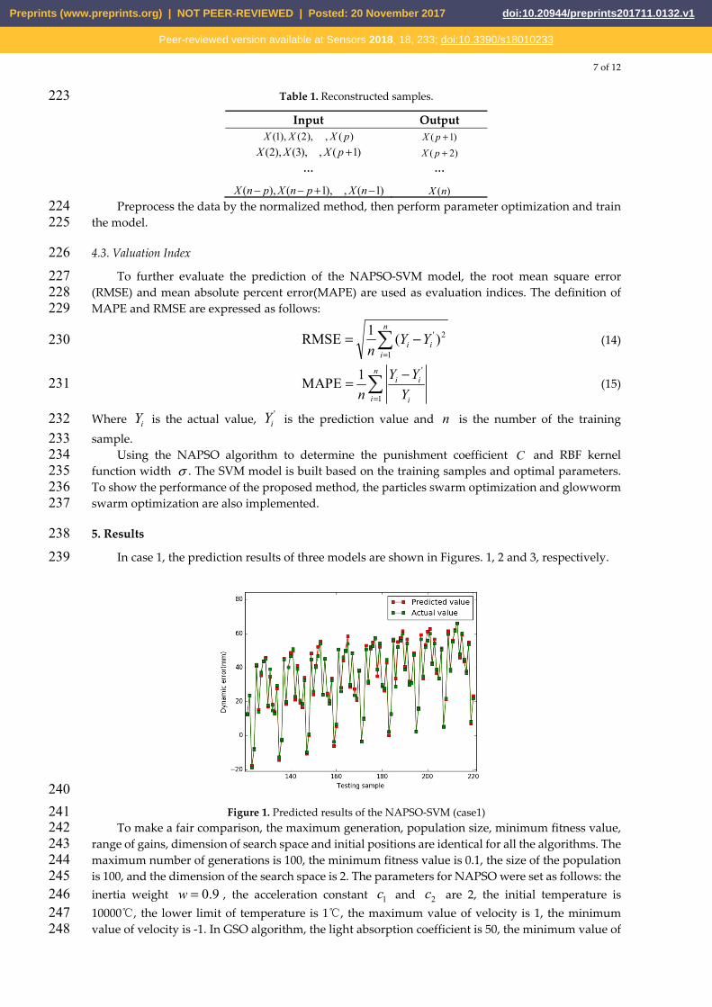
5. Results 238 In case 1, the prediction results of three models are shown in Figures. 1, 2 and 3, respectively. 239

240 Figure 1. Predicted results of the NAPSO-SVM (case1) 241

To make a fair comparison, the maximum generation, population size, minimum fitness value, 242 range of gains, dimension of search space and initial positions are identical for all the algorithms. The 243 maximum number of generations is 100, the minimum fitness value is 0.1, the size of the population 244 is 100, and the dimension of the search space is 2. The parameters for NAPSO were set as follows: the 245 inertia weight 9.0=w , the acceleration constant 1c and 2c are 2, the initial temperature is 246 10000℃, the lower limit of temperature is 1℃, the maximum value of velocity is 1, the minimum 247 value of velocity is -1. In GSO algorithm, the light absorption coefficient is 50, the minimum value of 248




http://dx.doi.org/10.3390/s18010233

8 of 12

attractiveness is 0.8, the maximum value of attractiveness is 1.0, the value of initial step size factor is 249 0.5. The PSO algorithm has the same inertia weight and acceleration constant as the NAPSO 250 algorithm. 251

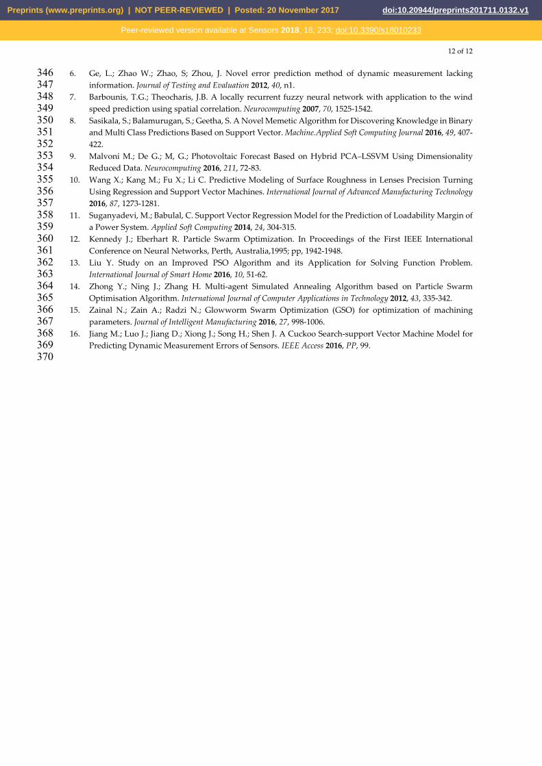
Figure.4 presents the comparison results of predicted residuals by the three models. The MAPE 252 value and RMSE value of the three models are listed in Table 2. 253

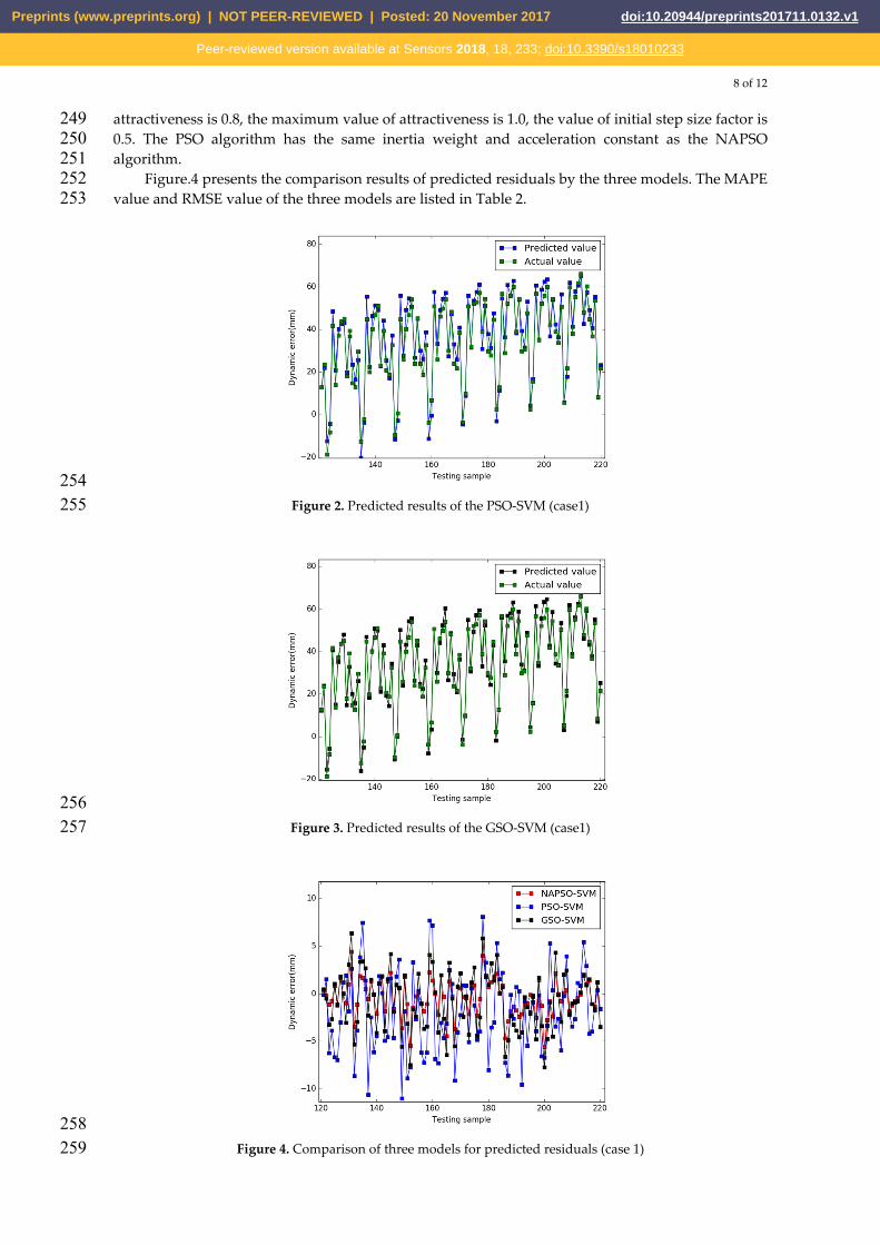
254 Figure 2. Predicted results of the PSO-SVM (case1) 255

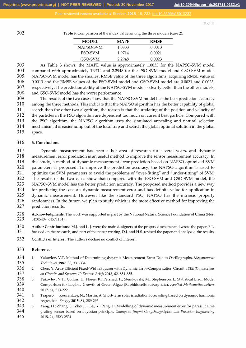
256 Figure 3. Predicted results of the GSO-SVM (case1) 257

258 Figure 4. Comparison of three models for predicted residuals (case 1) 259




http://dx.doi.org/10.3390/s18010233

9 of 12

By comparing Figures. 1-3, we find that the NAPSO-SVM model outperforms the PSO-SVM and 260 GSO-SVM model. The prediction performance of NAPSO-SVM is better than GSO-SVM model and 261 accuracy much better than PSO-SVM. 262

The residual curves of the three models are shown in the Figure. 4, The prediction residual curve 263 of the PSO-SVM model is large, ranging from -11 to ''8 , and the prediction residual of the GSO-SVM 264 model is smaller than the PSO-SVM model. But it is still relatively large, ranging from -8 to ' '6 . The 265 predicted residual of the NAPSO-SVM is smaller than the others and tends to more gentle, ranging 266 from -5 to ''4 .The results prove that dynamic measurement error prediction ability of NAPSO-SVM 267 model is better than PSO-SVM and GSO-SVM model, and the NAPSO algorithm is an effective 268 method for parameters optimization. 269

To further verify the ability of the three models. Table 2 lists the comparison results between the 270 three models for prediction accuracy indexes. 271

Table 2. Comparison of the index value among the three models (case 1). 272 MODEL MAPE RMSE

NAPSO-SVM 0.0744 0.1879 PSO-SVM 0.2423 0.4710 GSO-SVM 0.1493 0.3128

In Table 2, the MAPE value and RMSE value of the NAPSO-SVM model are smaller than the 273 PSO-SVM and GSO-SVM model. The MAPE value is approximately 0.0744 for NAPSO-SVM model 274 compared with approximately 0.2423 and 0.1493 for the PSO-SVM and GSO-SVM model, respectively. 275 Furthermore, the RMSE value is 0.1876 in the case of NAPSO-SVM model. Compared with the 276 NAPSO-SVM model, the RMSE value of the GSO-SVM model and PSO-SVM model are 0.4710 and 277 0.3128 respectively. In summary, the results of the Table 2 are accorded with the Figure. 4, the 278 NAPSO-SVM model has the best dynamic measurement error prediction ability among the three 279 methods. 280

In case 2, the parameters of each algorithm are essentially the same as the previous case, the 281 prediction results of three models are shown in Figures.5, 6 and 7. Figure.8 shows the comparison 282 results of predicted residuals by three models. The MAPE value and RMSE value of the three models 283 are listed in the Table 3. 284

285 Figure 5. Predicted results of the NAPSO-SVM (case 2) 286

In Figures.5-7, when the ratio of training samples and testing samples is approximately 3.5, the 287 prediction curve of the NAPSO-SVM model is closest to the actual value curve, and the prediction 288 curve of the NAPSO-SVM model is approximately the same as the actual value curve. However, 289 unlike the case 1, The prediction results of the PSO-SVM model is better than the PSO-SVM model, 290 but the prediction curves of these two models still lag behind the actual value curve. 291




http://dx.doi.org/10.3390/s18010233

10 of 12

292 Figure 6. Predicted results of the PSO-SVM (case 2) 293

294 Figure 7. Predicted results of the GSO-SVM (case2) 295

296 Figure 8. Comparison of the predicted residuals of the three models(case2) 297

In Figure.8, the prediction residual of the NAPSO-SVM model is smallest among the three 298 models, ranging from -0.013 to 0.014 mm. The prediction residual of the GSO-SVM model is ranging 299 from -0.035 to 0.026 mm, and the prediction residual of the PSO-SVM model is ranging from -0.032 300 to 0.013 mm. 301




http://dx.doi.org/10.3390/s18010233

11 of 12

Table 3. Comparison of the index value among the three models (case 2). 302 MODEL MAPE RMSE

NAPSO-SVM 1.0833 0.0013 PSO-SVM 1.9714 0.0021 GSO-SVM 2.2948 0.0023

As Table 3 shows, the MAPE value is approximately 1.0833 for the NAPSO-SVM model 303 compared with approximately 1.9714 and 2.2948 for the PSO-SVM model and GSO-SVM model. 304 NAPSO-SVM model has the smallest RMSE value of the three algorithms, acquiring RMSE value of 305 0.0013 and the RMSE values of the PSO-SVM model and GSO-SVM model are 0.0021 and 0.0023, 306 respectively. The prediction ability of the NAPSO-SVM model is clearly better than the other models, 307 and GSO-SVM model has the worst performance. 308

The results of the two cases show that the NAPSO-SVM model has the best prediction accuracy 309 among the three methods. This indicate that the NAPSO algorithm has the better capability of global 310 search than the other two algorithm, the reason is that the updating of the position and velocity of 311 the particles in the PSO algorithm are dependent too much on current best particle. Compared with 312 the PSO algorithm, the NAPSO algorithm uses the simulated annealing and natural selection 313 mechanism, it is easier jump out of the local trap and search the global optimal solution in the global 314 space. 315

6. Conclusions 316 Dynamic measurement has been a hot area of research for several years, and dynamic 317

measurement error prediction is an useful method to improve the sensor measurement accuracy. In 318 this study, a method of dynamic measurement error prediction based on NAPSO-optimized SVM 319 parameters is proposed. To improve the prediction accuracy, the NAPSO algorithm is used to 320 optimize the SVM parameters to avoid the problems of “over-fitting” and “under-fitting” of SVM. 321 The results of the two cases show that compared with the PSO-SVM and GSO-SVM model, the 322 NAPSO-SVM model has the better prediction accuracy. The proposed method provides a new way 323 for predicting the sensor’s dynamic measurement error and has definite value for application in 324 dynamic measurement. However, like the standard PSO, NAPSO has the intrinsic property 325 randomness. In the future, we plan to study which is the more effective method for improving the 326 prediction results. 327 Acknowledgments: The work was supported in part by the National Natural Science Foundation of China (Nos. 328 51305407, 61571104). 329 Author Contributions:. M.J. and L. J. were the main designers of the proposed scheme and wrote the paper. F.L. 330 focused on the research, and part of the paper writing, D.J. and H.S. revised the paper and analyzed the results. 331 Conflicts of Interest: The authors declare no conflict of interest. 332

References 333 1. Yakovlev, V.T. Method of Determining dynamic Measurement Error Due to Oscillographs. Measurement 334

Techniques 1987, 30, 331-334. 335 2. Chen, Y. Area-Efficient Fixed-Width Squarer with Dynamic Error-Compensation Circuit. IEEE Transactions 336

on Circuits and Systems II: Express Briefs 2015, 62, 851-855. 337 3. Yakovlev, V.T.; Collins, E.; Flores, K.; Pershad, P.; Stemkovski, M.; Stephenson, L. Statistical Error Model 338

Comparison for Logistic Growth of Green Algae (Raphidocelis subcapitata). Applied Mathematics Letters 339 2017, 64, 213-222. 340

4. Trapero, J.; Kourentzes, N.; Martin, A. Short-term solar irradiation forecasting based on dynamic harmonic 341 regression. Energy 2015, 84, 289-295. 342

5. Yang, H.; Zhang, L.; Zhou, J.; Fei, Y.; Peng, D. Modelling of dynamic measurement error for parasitic time 343 grating sensor based on Bayesian principle. Guangxue Jingmi Gongcheng/Optics and Precision Engineering 344 2015, 24, 2523-2531. 345




http://dx.doi.org/10.3390/s18010233

12 of 12

6. Ge, L.; Zhao W.; Zhao, S; Zhou, J. Novel error prediction method of dynamic measurement lacking 346 information. Journal of Testing and Evaluation 2012, 40, n1. 347

7. Barbounis, T.G.; Theocharis, J.B. A locally recurrent fuzzy neural network with application to the wind 348 speed prediction using spatial correlation. Neurocomputing 2007, 70, 1525-1542. 349

8. Sasikala, S.; Balamurugan, S.; Geetha, S. A Novel Memetic Algorithm for Discovering Knowledge in Binary 350 and Multi Class Predictions Based on Support Vector. Machine.Applied Soft Computing Journal 2016, 49, 407-351 422. 352

9. Malvoni M.; De G.; M, G.; Photovoltaic Forecast Based on Hybrid PCA–LSSVM Using Dimensionality 353 Reduced Data. Neurocomputing 2016, 211, 72-83. 354

10. Wang X.; Kang M.; Fu X.; Li C. Predictive Modeling of Surface Roughness in Lenses Precision Turning 355 Using Regression and Support Vector Machines. International Journal of Advanced Manufacturing Technology 356 2016, 87, 1273-1281. 357

11. Suganyadevi, M.; Babulal, C. Support Vector Regression Model for the Prediction of Loadability Margin of 358 a Power System. Applied Soft Computing 2014, 24, 304-315. 359

12. Kennedy J.; Eberhart R. Particle Swarm Optimization. In Proceedings of the First IEEE International 360 Conference on Neural Networks, Perth, Australia,1995; pp, 1942-1948. 361

13. Liu Y. Study on an Improved PSO Algorithm and its Application for Solving Function Problem. 362 International Journal of Smart Home 2016, 10, 51-62. 363

14. Zhong Y.; Ning J.; Zhang H. Multi-agent Simulated Annealing Algorithm based on Particle Swarm 364 Optimisation Algorithm. International Journal of Computer Applications in Technology 2012, 43, 335-342. 365

15. Zainal N.; Zain A.; Radzi N.; Glowworm Swarm Optimization (GSO) for optimization of machining 366 parameters. Journal of Intelligent Manufacturing 2016, 27, 998-1006. 367

16. Jiang M.; Luo J.; Jiang D.; Xiong J.; Song H.; Shen J. A Cuckoo Search-support Vector Machine Model for 368 Predicting Dynamic Measurement Errors of Sensors. IEEE Access 2016, PP, 99. 369 370




http://dx.doi.org/10.3390/s18010233

dynamic measurement errors prediction model of sensors

Documents