Dynamic factor models

Jörg Breitung(University of Bonn and Deutsche Bundesbank)

Sandra Eickmeier(Deutsche Bundesbank and University of Cologne)

Discussion PaperSeries 1: Economic StudiesNo 38/2005Discussion Papers represent the authors’ personal opinions and do not necessarily reflectthe views of the Deutsche Bundesbank or its staff.

Editorial Board: Heinz Herrmann Thilo Liebig Karl-Heinz Tödter Deutsche Bundesbank, Wilhelm-Epstein-Strasse 14, 60431 Frankfurt am Main, Postfach 10 06 02, 60006 Frankfurt am Main Tel +49 69 9566-1 Telex within Germany 41227, telex from abroad 414431, fax +49 69 5601071 Please address all orders in writing to: Deutsche Bundesbank, Press and Public Relations Division, at the above address or via fax +49 69 9566-3077

Reproduction permitted only if source is stated.

ISBN 3–86558–097–1

Abstract: Factor models can cope with many variables without running into scarce degrees of freedom problems often faced in a regression-based analysis. In this article we review recent work on dynamic factor models that have become popular in macroeconomic policy analysis and forecasting. By means of an empirical application we demonstrate that these models turn out to be useful in investigating macroeconomic problems. Keywords: Principal components, dynamic factors, forecasting

JEL Classification: C13, C33, C51

Non technical summary In recent years, large-dimensional dynamic factor models have become popular in empirical macroeconomics. They are more advantageous than other methods in various respects. Factor models can cope with many variables without running into scarce degrees of freedom problems often faced in regression-based analyses. Researchers and policy makers nowadays have more data at a more disaggregated level at their disposal than ever before. Once collected, the data can be processed easily and rapidly owing to the now wide-spread use of high-capacity computers. Exploiting a lot of information can lead to more precise forecasts and macroeconomic analyses. A second advantage of factor models is that idiosyncratic movements which possibly include measurement error and local shocks can be eliminated. This yields a more reliable signal for policy makers and prevents them from reacting to idiosyncratic movements. In addition, the estimation of common factors or common shocks is of intrinsic interest in some applications. A third important advantage is that factor modelers can remain agnostic about the structure of the economy and do not need to rely on overly tight assumptions as is sometimes the case in structural models. It also represents an advantage over structural VAR models where the researcher has to take a stance on the variables to include which, in turn, determine the outcome, and where the number of variables determine the number of shocks. In this article we review recent work on dynamic factor models and illustrate the concepts with an empirical example. We start by considering the traditional factor model. This model is designed to handle data sets which include only a small number of variables, and in this type of model, it is not allowed for serial and mutual correlation of the idiosyncratic errors. These fairly restrictive assumptions can be relaxed if it is assumed that the number of variables tends to infinity. Large data sets can be dealt with by the approximate factor model, which is outlined in this paper. We discuss different test procedures for determining the number of factors. Finally we present the dynamic factor model which allows the common factors to affect the variables not only contemporaneously, but also with lags. In addition, the factors may be described as a VAR model which is useful for structural macroeconomic analysis. The article gives an overview of recent empirical work based on dynamic factor models. Those were traditionally used to construct economic indicators and to forecast. More recently, dynamic factor models were also employed to analyze monetary policy and international business cycles. We finally estimate a dynamic factor model for a large set of macroeconomic variables from European monetary union (EMU) member countries and central and eastern European countries (CEECs). We find that the variance shares of output growth explained by the common factors are larger in most EMU countries than in the CEECs. However, the variance shares associated with output growth in several CEECs exceed those associated with

some peripheral EMU countries like Greece and Portugal, the latter being encouraging from the point of view of the prospective accession of the CEECs to EMU.

Nicht technische Zusammenfassung

In den letzten Jahren haben große dynamische Faktormodelle in der empirischen

Makroökonomik an Bedeutung gewonnen. Sie weisen gegenüber anderen Methoden

verschiedene Vorteile auf. Faktormodelle können viele Variablen einbeziehen, ohne dass das

bei der Regressionsanalyse häufig auftretende Problem der unzureichenden Freiheitsgrade

akut wird. Der Forschung und der Politik stehen heutzutage mehr und stärker disaggregierte

Daten zur Verfügung als je zuvor. Die erhobenen Daten können aufgrund des inzwischen

verbreiteten Einsatzes leistungsstarker Computer leicht und rasch bearbeitet werden. Auf der

Grundlage umfangreicherer Datensätze lassen sich präzisere Prognosen und aussagefähigere

makroökonomische Analysen erstellen. Ein zweiter Vorteil von Faktormodellen liegt darin,

dass sich idiosynkratische, das heißt variablen-spezifische, Bewegungen herausrechnen

lassen, die möglicherweise auf Messfehlern und lokalen Schocks beruhen. Damit erhalten die

Politiker ein verlässlicheres Signal, und es kann verhindert werden, dass sie auf

idiosynkratische Entwicklungen reagieren. Darüber hinaus ist die Schätzung gemeinsamer

Faktoren oder Schocks für einige Anwendungen von eigenständigem Interesse. Ein dritter

wichtiger Vorteil besteht darin, dass Faktormodelle eine agnostische Betrachtung der

Wirtschaftsstruktur ermöglichen und keine zu strengen Annahmen erfordern, wie es zuweilen

bei strukturellen Modellen der Fall ist. Außerdem besteht ein Vorteil gegenüber strukturellen

VAR-Modellen, bei denen sich der Forscher für bestimmte Variablen entscheiden muss,

deren Auswahl das Ergebnis beeinflusst und deren Anzahl die Zahl der Schocks vorgibt.

Das vorliegende Papier beschäftigt sich mit jüngeren Untersuchungen zu dynamischen

Faktormodellen und veranschaulicht die Konzepte anhand eines empirischen Beispiels.

Zunächst wird das klassische Faktormodell betrachtet. Dieses Modell dient der Analyse von

Datensätzen, die nur wenige Variablen umfassen, und dieser Modelltyp schließt eine serielle

und gegenseitige Korrelation der idiosynkratischen Fehler aus. Diese recht restriktiven

Annahmen können gelockert werden, wenn angenommen wird, dass die Anzahl der Variablen

gegen unendlich geht. Umfangreiche Datensätze können mithilfe des in diesem

Diskussionspapier beschriebenen approximativen Faktormodells analysiert werden. Es

werden unterschiedliche Testverfahren zur Bestimmung der Faktoranzahl diskutiert.

Schließlich wird ein dynamisches Faktormodell vorgestellt, bei dem die gemeinsamen

Faktoren die Variablen nicht nur kontemporär, sondern auch verzögert beeinflussen können.

Zudem lassen sich die Faktoren auch als VAR-Modell darstellen, was für die strukturelle

makroökonomische Analyse nützlich ist.

Das vorliegende Papier gibt einen Überblick über neuere empirische Untersuchungen auf der

Grundlage dynamischer Faktormodelle. Diese Modelle wurden in der Vergangenheit meist

zur Konstruktion ökonomischer Indikatoren und zur Prognose verwendet. In jüngerer Zeit

wurden dynamische Faktormodelle auch zur Analyse der Geldpolitik und internationaler

Konjunkturzyklen herangezogen. In diesem Diskussionspapier wird ein dynamisches

Faktormodell für eine große Anzahl makroökonomischer Variablen aus den Mitgliedstaaten

der Europäischen Währungsunion (EWU) und der mittel- und osteuropäischen Länder (MOE)

geschätzt. Wir kommen zu dem Ergebnis, dass die Varianzanteile des Produktionszuwachses,

die von den gemeinsamen Faktoren erklärt werden, in den meisten EWU-Ländern größer sind

als in den MOE. Allerdings sind die Varianzanteile des Produktionszuwachses in einigen

mittel- und osteuropäischen Volkswirtschaften größer als in einigen peripheren EWU-

Mitgliedstaaten (etwa Griechenland und Portugal), was für den angestrebten Beitritt der MOE

zur EWU eine gute Voraussetzung ist.

Contents

1 Introduction 1

2 The strict factor model 2

3 Approximate factor models 4

4 Specifying the number of factors 5

5 Dynamic factor models 6

6 Overview of existing applications 8

7 An empirical example 10

8 Conclusion 13

Bibliography 13

Tables and Figures

Table 1 Criteria for selecting the number of factors 17

Table 2 Variance shares explained by the common factors 17

Figure 1 Euro-area business cycle estimates 18

Dynamic Factor Models∗

1 Introduction

In recent years, large-dimensional dynamic factor models have become popular

in empirical macroeconomics. They are more advantageous than other methods

in various respects. Factor models can cope with many variables without running

into scarce degrees of freedom problems often faced in regression-based analyses.

Researchers and policy makers nowadays have more data at a more disaggregated

level at their disposal than ever before. Once collected, the data can be processed

easily and rapidly owing to the now wide-spread use of high-capacity computers.

Exploiting a lot of information can lead to more precise forecasts and macroe-

conomic analyses. The use of many variables further reflects a central bank’s

practice of ”looking at everything” as emphasized, for example, by Bernanke

and Boivin (2003). A second advantage of factor models is that idiosyncratic

movements which possibly include measurement error and local shocks can be

eliminated. This yields a more reliable signal for policy makers and prevents

them from reacting to idiosyncratic movements. In addition, the estimation of

common factors or common shocks is of intrinsic interest in some applications. A

third important advantage is that factor modellers can remain agnostic about the

structure of the economy and do not need to rely on overly tight assumptions as

is sometimes the case in structural models. It also represents an advantage over

structural VAR models where the researcher has to take a stance on the vari-

ables to include which, in turn, determine the outcome, and where the number

of variables determine the number of shocks.

In this article we review recent work on dynamic factor models and illustrate

the concepts with an empirical example. In Section 2 the traditional factor model

is considered and the approximate factor model is outlined in Section 3. Different

test procedures for determining the number of factors are discussed in section

4. The dynamic factor model is considered in Section 5. Section 6 gives an

overview of recent empirical work based on dynamic factor models and Section 7

∗Affiliations: University of Bonn and Deutsche Bundesbank (Jorg Breitung), DeutscheBundesbank and University of Cologne (Sandra Eickmeier). Corresponding address: Insti-tute of Econometrics, University of Bonn, Adenauerallee 24-42, 53113 Bonn, Germany, Email:breitung@uni-bonn.de.

1

presents the results of estimating a large-scale dynamic factor model for a large

set of macroeconomic variables from European monetary union (EMU) member

countries and central and eastern European countries (CEECs). Finally, Section

8 concludes.

2 The strict factor model

In an r-factor model each element of the vector yt = [y1t, . . . , yNt]′ can be repre-

sented as

yit = λi1f1t + · · ·+ λirfrt + uit , t = 1, . . . , T

= λ′i·ft + uit ,

where λ′i· = [λi1, . . . , λir] and ft = [f1t, . . . , frt]′. The vector ut = [u1t, . . . , uNt]

′

comprises N idiosyncratic components and ft is a vector of r common factors.

In matrix notation the model is written as

yt = Λft + ut

Y = FΛ′ + U,

where Λ = [λ1·, . . . , λN ·]′, Y = [y1, . . . , yT ]

′, F = [f1, . . . , fT ]′ and U = [u1, . . . , uT ]

′.

For the strict factor model it is assumed that ut is a vector of mutually un-

correlated errors with E(ut) = 0 and E(utu′

t) = Σ = diag(σ21, . . . , σ

2N ). For the

vector of common factors we assume E(ft) = 0 and E(ftf′

t) = Ω.1 Furthermore,

E(ftu′

t) = 0. From these assumptions it follows that2

Ψ = E(yty′

t) = ΛΩΛ′ + Σ.

The loading matrix Λ can be estimated by minimizing the residual sum of squares:

T∑

t=1

(yt −Bft)′(yt −Bft) (1)

subject to the constraint B ′B = Ir. Differentiating (1) with respect to B and

F yields the first order condition (µIN − S)βk = 0 for k = 1, . . . , r, where S =

1That is we assume that E(yt) = 0. In practice, the means of the variables are subtractedto obtain a vector of mean zero variables.

2In many applications the correlation matrix is used instead of the covariance matrix of yt.This standardization affects the properties of the principal component estimator, whereas theML estimator is invariant with respect to a standardization of the variables.

2

T−1∑T

t=1yty

′

t and βi is the i’th column of B, the matrix that minimizes the

criterion function (1). Thus, the columns of B result as the eigenvectors of the r

largest eigenvalues of the matrix S. The matrix B is the Principal Components

(PC) estimator of Λ.

To analyse the properties of the PC estimator it is instructive to rewrite the

PC estimator as an IV estimator. The PC estimator can be shown to solve the

following moment condition:

T∑

t=1

B′ytu′

t = 0, (2)

where ut = B′

⊥yt and B⊥ is an N × (N − r) orthogonal complement of B such

that B′

⊥B = 0. Specifically,

B⊥ = IN − B(B′B)−1B′ = IN − BB′

where we have used the fact that B′B = Ir. Therefore, the moment condition

can be written as∑N

t=1ftu

′

t, where ut = yt − B′ft and ft = B′yt. Since the

components of ft are linear combinations of yt, the instruments are correlated

with ut, in general. Therefore, the PC estimator is inconsistent for fixed N and

T →∞ unless Σ = σ2I.3

An alternative representation that will give rise to a new class of IV estimators

is given by choosing a different orthogonal complement B⊥. Let Λ = [Λ′

1,Λ′

2]′

such that Λ1 and Λ2 are (N − r) × r and r × r submatrices, respectively. The

matrix U = [u1, . . . , uN ]′ is partitioned accordingly such that U = [U ′

1, U′

2] and

U1 (U2) are T × (N − r) (T × r) submatrices. A system of equations results from

solving Y2 = FΛ′

2 +U2 for F and inserting the result in the first set of equations:

Y1 = (Y2 − U2)(Λ′

2)−1Λ′

1 + U1

= Y2Θ′ + V (3)

where Θ = Λ1Λ−1

2 and V = U1−U2Θ′. Accordingly Θ yields an estimator for the

renormalized loading matrix B∗ = [Θ′, Ir]′ and B∗

⊥= [Ir,Θ

′]′.

The i’th equation of system (3) can be consistently estimated based on the

following N − r − 1 moment conditions

E(yktvit) = 0, k = 1, . . . , i− 1, i+ 1, . . . , N − r (4)

3To see that the PC estimator yields a consistent estimator of the factor space for Σ = σ2IN

let B denote the matrix of r eigenvectors of Ψ. It follows that B ′ΨB⊥ = B′ΛΩΛ′B⊥. Thelatter expression becomes zero if B = ΛQ, where Q is some regular r × r matrix.

3

that is, we do not employ yit and yn+1,t, . . . , yNt as instruments as they are cor-

related with vit. Accordingly, a GMM estimator based on (N − r)(N − r − 1)

moment conditions can be constructed to estimate the n · r parameters in the

matrix Θ. An important problem with this estimator is that the number of in-

struments increases rapidly as N increases. It is well known that, if the number

of instruments is large relative to the number of observations, the GMM esti-

mator may have poor properties in small samples. Furthermore, if n2 − n > T ,

the weight matrix for the GMM estimator is singular. Therefore it is desirable

to construct a GMM estimator based on a smaller number of instruments. Bre-

itung (2005) proposes a just-identified IV etimator based on equation specific

instruments that do not involve yit and yn+1,t, . . . , yNt.

In the case of homogeneous variances (i.e. Σ = σ2IN) the PC estimator is the

maximum likelihood (ML) estimator assuming that yt is normally distributed.

In the general case with Σ = diag(σ21, . . . , σ

2N) the ML estimator minimizes the

function `∗ = tr(SΣ−1)+log |Σ| (cf. Joreskog 1969). Various iterative procedures

have been suggested to compute the ML estimator from the set of highly nonlinear

first order conditions. For large factor models (with N > 20, say) it has been

observed that the convergence of the usual maximization algorithms is quite slow

and in many cases the algorithms have difficulty in converging to the global

maximum.

3 Approximate factor models

The fairly restrictive assumption of the strict factor model can be relaxed if it

is assumed that the number of variables (N) tends to infinity (cf. Chamberlain

and Rothshield 1983, Stock and Watson 2002a and Bai 2003). First, it is possible

to allow for (weak) serial correlation of the idiosyncratic errors. Thus, the PC

estimator remains consistent if the idiosyncratic errors are generated by (possi-

bly different) stationary ARMA processes. However, persistent and non-ergodic

processes such as the random walk are ruled out. Second, the idiosyncratic errors

may be weakly cross-correlated and heteroskedastic. This allows for finite “clus-

ters of correlation” among the errors. Another way to express this assumption

is to assume that all eigenvalues of E(utu′

t) = Σ are bounded. Third, the model

allows for weak correlation among the factors and the idiosyncratic components.

Finally, N−1Λ′Λ must converge to a positive definite limiting matrix. Accord-

ingly, on average the factors contribute to all variables with a similar order of

4

magnitude. This assumption rules out the possibility that the factors contribute

only to a limited number of variables, whereas for an increasing number of re-

maining variables the loadings are zero.

Beside these assumptions a number of further technical assumptions restrict

the moments of the elements of the random vectors ft and ut. With these as-

sumptions Bai (2003) establishes the consistency and asymptotic normality of the

PC estimator for Λ and ft. However, as demonstrated by Bovin and Ng (2005a)

the small sample properties may be severely affected when (a part of) the data

is cross-correlated.

4 Specifying the number of factors

In practice, the number of factors necessary to represent the correlation among

the variables is usually unknown. To determine the number of factors empiri-

cally a number of criteria were suggested. First, the eigenvalues of the sample

correlation matrix R may roughly indicate the number of common factors. Since

tr(R) = N =∑N

i=1µi, where µi denotes the i’th eigenvalue of R (in descend-

ing order), the fraction of the total variance explained by k common factors is

τ(k) = (∑k

i=1µi)/N . Unfortunately, there is no generally accepted limit for the

explained variance that indicates a sufficient fit. Sometimes it is recommended

to include those factors with an eigenvalue larger than unity, since these factors

explain more than an “average factor”.

In some applications (typically in psychological or sociological studies) two or

three factors explain more than 90 percent of the variables, whereas in macroe-

conomic panels a variance ratio of 40 percent is sometimes considered as a rea-

sonable fit.

A related method is the “Scree-test”. Cattell (1966) observed that the graph

of the eigenvalues (in descending order) of an uncorrelated data set forms a

straight line with an almost horizontal slope. Therefore, the point in the eigen-

value graph where the eigenvalues begin to level off with a flat and steady decrease

is an estimator of the sufficient number of factors. Obviously such a criterion is

often fairly subjective because it is not uncommon to find more than one major

break in the eigenvalue graph and there is no unambiguous rule to use.

Several more objective criteria based on statistical tests are available that

can be used to determine the number of common factors. If it is assumed that

r is the true number of common factors, then the idiosyncratic components ut

5

should be uncorrelated. Therefore it is natural to apply tests that are able to

indicate a contemporaneous correlation among the elements of ut. The score test

is based on the sum of all relevant N(N − 1)/2 squared correlations. This test

is asymptotically equivalent to the LR test based on (two times) the difference

of the log-likelihood of the model assuming r0 factors against a model with an

unrestricted covariance matrix. An important problem of these tests is that they

require T >> N >> r. Otherwise the performance of these tests is quite poor.

Therefore, in typical macroeconomic panels which include more than 50 variables

these tests are not applicable.

For the approximate factor model Bai and Ng (2002) have suggested informa-

tion criteria that can be used to estimate the number of factors consistently as N

and T tend to infinity. Let V (k) = (NT )−1∑T

t=1u′tut denote the (overall) sum of

squared residuals from a k-factor model, where ut = yt− Bft is the N × 1 vector

of estimated idiosyncratic errors. Bai and Ng (2002) suggest several variants of

the information criterion, where the most popular statistic is

ICp2(k) = ln[V (k)] + k

(N + T

NT

)ln[minN, T].

The estimated number of factors (k) is obtained from minimizing the information

criterion in the range k = 0, 1, . . . , kmax where kmax is some pre-specified upper

bound for the number of factors. As N and T tend to infinity, kp→ r, i.e., the

criterion is (weakly) consistent.

An alternative procedure to determine the number of factors based on the

empirical distribution of the eigenvalues is recently suggested by Onatski (2005).

5 Dynamic factor models

The dynamic factor model is given by

yt = Λ0gt + Λ1gt−1 + · · ·+ Λmgt−m + ut (5)

where Λ0, . . . ,Λm are N × r matrices and gt is a vector of q stationary factors.

As before, the idiosyncratic components of ut are assumed to be independent (or

weakly dependent) stationary processes.

Forni, Giannone, Lippi and Reichlin (2004) suggest an estimation proce-

dure of the innovations of the factors ηt = gt − E(gt|gt−1, gt−2, . . .). Let ft =

[g′t, g′

t−1, . . . , g′

t−m]′ denote the r = (m+ 1)q vector of “static” factors such that

yt = Λ∗ft + ut , (6)

6

where Λ∗ = [Λ0, . . . ,Λm]. In a first step the static factors ft are estimated by PC.

Let ft denote the vector of estimated factors. It is important to note that a (PC)

estimator does not estimate the original vector ft but some “rotated” vector Qft

such that the components of (Qft) are orthogonal. In a second step a VAR model

is estimated:

ft = A1ft−1 + · · ·+ Apft−p + et . (7)

Since ft includes estimates of the lagged factors, some of the VAR equations

are identities (at least asymptotically) and, therefore, the rank of the residual

covariance matrix Σe = T−1∑T

t=p+1ete

′

t is q, as N → ∞. Let Wr denote the

matrix of q eigenvectors associated with the q largest eigenvalues of Σe. The

estimate of the innovations of the dynamic factors results as ηt = W ′

ret. These

estimates can be used to identify structural shocks that drive the common factors

(cf. Forni et al. 2004, Giannone, Sala and Reichlin 2002).

An important problem is to determine the number of dynamic factors q from

the vector of r static factors. Forni et al. (2004) suggest an informal criterion

based on the portion of explained variances, whereas Bai and Ng (2005) and Stock

and Watson (2005) suggest consistent selection procedures based on principal

components. Breitung and Kretschmer (2005) propose a test procedure based

on the canonical correlation between ft and ft−1. The i’th eigenvalue from a

canonical correlation analysis can be seen as an R2 from a regression of v′ift on

ft−1, where vi denotes the associated eigenvector. If there is a linear combination

of ft that corresponds to a lagged factor, then this linear combination is perfectly

predictable and, therefore, the corresponding R2 (i.e. the eigenvalue) will tend to

unity. On the other hand, if the linear combination reproduces the innovations of

the original factor, then this linear combination is not predictable and, therefore,

the eigenvalue will tend to zero. Based on this reasoning, information criteria and

tests of the number of factors are suggested by Breitung and Kretschmer (2005).

Forni et al. (2000, 2002) suggest an estimator of the dynamic factors in the

frequency domain. This estimator is based on the frequency domain representa-

tion of the factor model given by

fy(ω) = fχ(ω) + fu(ω),

where χt = Λ0ft + · · · + Λmft−m denotes the vector of common components of

yt, fχ is the associated spectral density matrix, fy is the spectral density matrix

of yt and ut is the (diagonal) spectral density matrix of ut. Dynamic principal

components analysis applied to the frequencies ω ∈ [0, π] (Brillinger 1981) yields

7

a consistent estimate of the spectral density matrix fχ(ω). An estimate of the

common components χit is obtained by computing the time domain representa-

tion of the process from an inversion of the spectral densities. The frequency

domain estimator yields a two-sided filter such that ft =∑

∞

j=−∞Ψ′

jyt−j, where,

in practice, the infinite limits are truncated. Forni, et al. (2005) also suggest

a one-sided filter which is based on a conventional principal component analysis

of the transformed vector yt = Σ−1/2yt, where Σ is the (frequency domain) es-

timate of the covariance matrix of ut. This one-sided estimator can be used for

forecasting based on the common factors.

6 Overview of existing applications

Dynamic factor models were traditionally used to construct economic indicators

and for forecasting. More recently, they have been applied to macroeconomic

analysis, mainly with respect to monetary policy and international business cy-

cles. We briefly give an overview of existing applications of dynamic factor models

in these four fields, before providing a macro analytic illustration.

Construction of economic indicators. The two most prominent examples of

monthly coincident business cycle indicators, to which policy makers and other

economic agents often refer, are the Chicago Fed National Activity Index4 (CF-

NAI) for the US and EuroCOIN for the euro area. The CFNAI estimate, which

dates back to 1967, is simply the first static principal component of a large macro

data set. It is the most direct successor to indicators which were first developed by

Stock and Watson but retired by the end of 2003. EuroCOIN is estimated as the

common component of euro-area GDP based on dynamic principal component

analysis. It was developed by Altissimo et al. (2001) and is made available from

1987 onwards by the CEPR.5 Measures of core inflation have been constructed

analogously (e.g. Cristadoro, Forni, Reichlin and Veronese (2001) for the euro

area and Kapetanios (2004) for the UK).

Forecasting. Factor models are widely used in central banks and research

institutions as a forecasting tool. The forecasting equation typically has the form

yht+h = µ+ a(L)yt + b(L)ft + eht+h , (8)

where yt is the variable to be forecasted at period t + h and et+h denotes the

h-step ahead prediction error. Accordingly, information used to forecast yt are

4See http://www.chicagofed.org/economic research and data/cfnai.cfm.5See http://www.cepr.org/data/eurocoin/.

8

the past of the variable and the common factor estimates ft extracted from an

additional data set.

Factor models have been used to predict real and nominal variables in the US

(e.g. Stock and Watson (2002a,b, 1999), Giacomini and White (2003), Banerjee

and Marcellino (2003)), in the euro area (e.g. Forni, Hallin, Lippi and Reich-

lin (2000, 2003), Camba-Mendez and Kapetanios (2004), Marcellino, Stock and

Watson (2003), Banerjee, Marcellino and Masten (2003)), for Germany (Schu-

macher and Dreger (2004), Schuhmacher 2005), for the UK (Artis, Banerjee and

Marcellino (2004)) and for the Netherlands (den Reijer 2005). The factor model

forecasts are generally compared to simple linear benchmark time series mod-

els, such as AR models, AR models with single measurable leading indicators

and VAR models. More recently, they have also been compared with pooled

single indicator forecasts or forecasts based on ”best” single indicator models or

groups of indicators derived using automated selection procedures (PCGets) (e.g.

Banerjee and Marcellino (2003)). Pooling variables versus combining forecasts is

a particularly interesting comparison, since both approaches claim to exploit a

lot of information.6

Overall, results are quite encouraging, and factor models are often shown to

be more successful in terms of forecasting performance than smaller benchmark

models. Three remarks are, however, in order. First, the forecasting performance

of factor models apparently depends on the types of variable one wishes to fore-

cast, the countries/regions of interest, the underlying data sets, the benchmark

models and horizons. Unfortunately, a systematic assessment of the determinants

of the relative forecast performance of factor models is still not available. Second,

it may not be sufficient to include just the first or the first few factors. Instead, a

factor which explains not much of the entire panel, say, the fifth or sixth principal

component, may be important for the variable one wishes to forecast (Banerjee

and Marcellino (2003)). Finally, the selection of the variables to be included in

the data set is ad hoc in most applications. The same data set is often used to

predict different variables. This may, however, not be adequate. Instead, one

should only include variables which exhibit high explanatory power with respect

to the variable that one aims to forecast (see also Bovin and Ng (2005b)).

Monetary policy analysis. Forni et al. (2004) and Giannone (2002, 2004)

6The models are further used to investigate the explanatory power of certain groups of vari-ables, for example financial variables (Forni et al. (2003)) or variables summarizing internationalinfluences for domestic activity (see, for example, Banerjee et al. (2003) who investigate theability of US variables or factors to predict euro-area inflation and output growth.

9

identify the main macroeconomic shocks in the US economy and estimate policy

rules conditional on the shocks. Sala (2003) investigates the transmission of com-

mon euro-area monetary policy shocks to individual EMU countries. Cimadomo

(2003) assesses the proliferation of economy-wide shocks to sectors in the US and

examines if systematic monetary policy has distributional and asymmetric effects

across sectors. All these studies rely on the structural dynamic factor model de-

veloped by Forni et al. (2004). Bernanke, Boivin and Eliasz (2005), Stock and

Watson (2005) and Favero, Marcellino and Neglia (2005) use a different but re-

lated approach. The two former papers address the problem of omitted variables

bias inherent in many simple small-scale VAR models. They show for the US that

the inclusion of factors in monetary VARs, denoted by factor-augmented VAR

(FAVAR) models, can eliminate the well-known price puzzle in the US. Favero

et al. (2005) confirm these findings for the US and for some individual euro-area

economies. They further demonstrate that the inclusion of factors estimated from

dynamic factor models in the instrument set used for estimation of Taylor rules

increases the precision of the parameters estimates.

International business cycles. Malek Mansour (2003) and Helbling and Bay-

oumi (2003) estimate a world and, respectively, a G7 business cycle and inves-

tigate to what extent the common cycle contributes to economic variation in

individual countries. Eickmeier (2004) investigates the transmission of structural

shocks from the US to Germany and assesses the relevance of the various trans-

mission channels and global shocks, thereby relying on the Forni et al. (2004)

framework. Marcellino, Stock and Watson (2000) and Eickmeier (2005) investi-

gate economic comovements in the euro-area. They try to give the common euro-

area factors an economic interpretation by relating them to individual countries

and variables using correlation measures.

7 An Empirical Example

Our application sheds some light on economic comovements in Europe by fitting

the large-scale dynamic factor model to a large set of macroeconomic variables

from European monetary union (EMU) member countries and central and east-

ern European countries (CEECs). We determine the dimension of the euro-area

economy, i.e. the number of macroeconomic driving forces which are common to

all EMU countries and which explain a significant share of the overall variance

in the set and we make some tentative interpretation. Most importantly, our

10

application addresses the recent discussion on whether the CEECs should join

the EMU. One of the criteria that should be satisfied is the synchronization of

business cycles. In what follows, we investigate how important euro-area fac-

tors are for the CEECs compared to the current EMU members. In addition,

the heterogeneity of the influences of the common factors across the CEECs is

examined.7

Our data set contains 41 aggregate euro-area time series, 20 key variables

of each of the core euro-area countries (Austria, Belgium, France, Germany,

Italy, Netherlands, Spain), real GDP and consumer prices for the remaining euro-

area economies (Finland, Greece, Ireland, Luxembourg, Portugal) and for eight

CEECs (Czech Republic, Estonia, Hungary, Lithuania, Latvia, Poland, Slovenia,

Slovak Republic) as well as some global variables.89 Overall, we include N = 208

quarterly series. The sample ranges from 1993Q1 to 2003Q4. The factor analysis

requires some pre-treatment of the data. Series exhibiting a seasonal pattern

were seasonally adjusted. Integrated series were made stationary through differ-

encing. Logarithms were taken of the series which were not in rates or negative,

and we removed outliers. We standardized the series to have a mean of zero and

a variance of one.

The series are collected in the vector N × 1 vector yt (t = 1, 2, . . . , T ). It

is assumed that yt follows an approximate dynamic factor model as described

in Section 3. The r common euro-area factors collected in ft are estimated by

applying static principal component analysis to the correlation matrix of yt. On

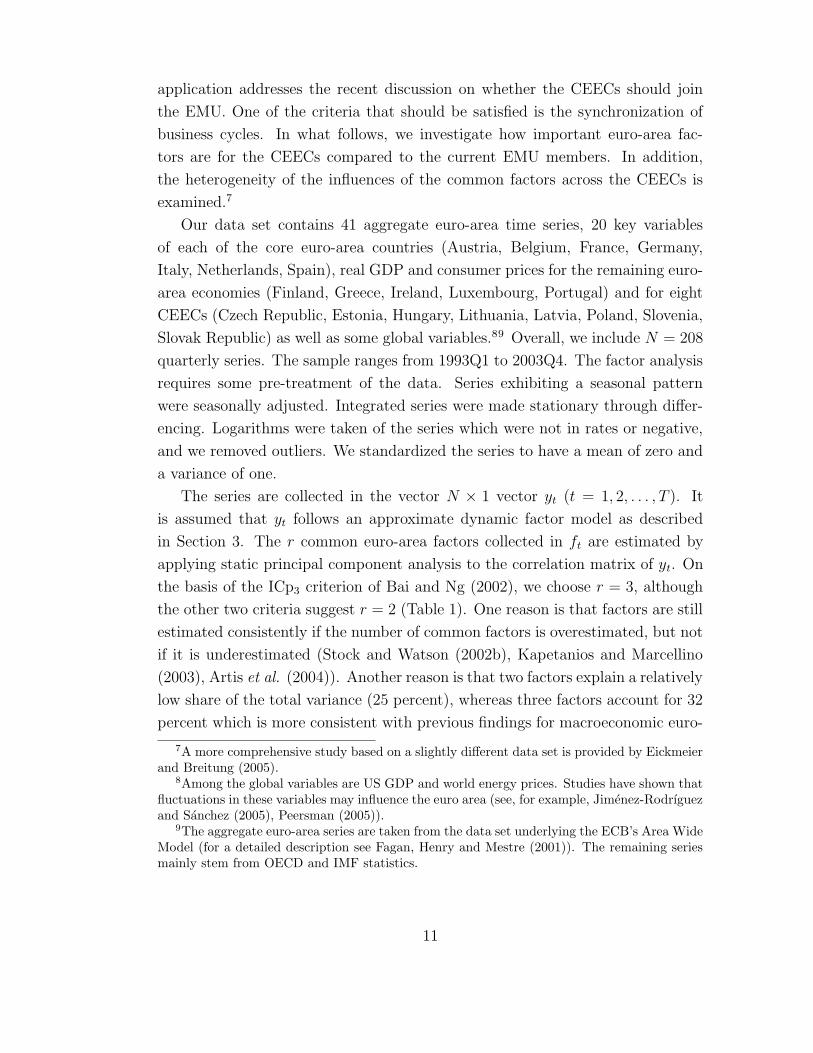
the basis of the ICp3 criterion of Bai and Ng (2002), we choose r = 3, although

the other two criteria suggest r = 2 (Table 1). One reason is that factors are still

estimated consistently if the number of common factors is overestimated, but not

if it is underestimated (Stock and Watson (2002b), Kapetanios and Marcellino

(2003), Artis et al. (2004)). Another reason is that two factors explain a relatively

low share of the total variance (25 percent), whereas three factors account for 32

percent which is more consistent with previous findings for macroeconomic euro-

7A more comprehensive study based on a slightly different data set is provided by Eickmeierand Breitung (2005).

8Among the global variables are US GDP and world energy prices. Studies have shown thatfluctuations in these variables may influence the euro area (see, for example, Jimenez-Rodrıguezand Sanchez (2005), Peersman (2005)).

9The aggregate euro-area series are taken from the data set underlying the ECB’s Area WideModel (for a detailed description see Fagan, Henry and Mestre (2001)). The remaining seriesmainly stem from OECD and IMF statistics.

11

area data sets (Table 1).10

The common factors ft do not bear a direct structural interpretation. One

reason is that ft may be a linear combination of the q ”true” dynamic factors and

their lags. Using the consistent Schwarz criterion of Breitung and Kretschmer

(2005), we obtain q = 2, conditional on r = 3. That is, one of the two static

factors enter the factor model with a lag. Informal criteria are also used in

practice. Two dynamic principal components explain 33 percent (Table 1). This

is comparable to the variance explained by the r static factors. The other criterion

consists in requiring each dynamic principal component to explain at least a

certain share, for example 10 percent, of the total variance. This would also

suggest q = 2.

Even if the dynamic factors were separated from their lags, they cannot be

given a direct economic meaning, since they are only identified up to a linear

transformation. Some tentative interpretation of the factors is given nevertheless.

In business cycle applications, the first factor is often interpreted as a common

cycle. Indeed, as is obvious from Figure 1, our first factor is highly correlated

with EuroCOIN and can therefore be interpreted as the euro-area business cycle.

To facilitate the interpretation of the other factors, the factors may be rotated to

obtain a new set of factors which satisfies certain identifying criteria, as done in

Eickmeier (2005). Another possibility consists in estimating the common struc-

tural shocks behind ft using structural vector autoregression (SVAR) and PC

techniques as suggested by Forni et al. (2004). This would also allow us to

investigate how common euro-area shocks spread to the CEECs.

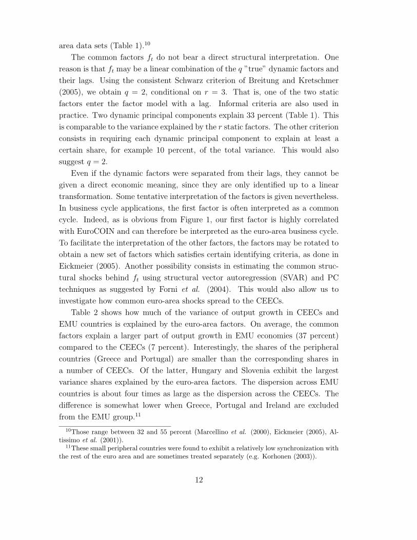
Table 2 shows how much of the variance of output growth in CEECs and

EMU countries is explained by the euro-area factors. On average, the common

factors explain a larger part of output growth in EMU economies (37 percent)

compared to the CEECs (7 percent). Interestingly, the shares of the peripheral

countries (Greece and Portugal) are smaller than the corresponding shares in

a number of CEECs. Of the latter, Hungary and Slovenia exhibit the largest

variance shares explained by the euro-area factors. The dispersion across EMU

countries is about four times as large as the dispersion across the CEECs. The

difference is somewhat lower when Greece, Portugal and Ireland are excluded

from the EMU group.11

10Those range between 32 and 55 percent (Marcellino et al. (2000), Eickmeier (2005), Al-tissimo et al. (2001)).

11These small peripheral countries were found to exhibit a relatively low synchronization withthe rest of the euro area and are sometimes treated separately (e.g. Korhonen (2003)).

12

8 Conclusion

In this paper we have reviewed and complemented recent work on dynamic factor

models. By means of an empirical application we have demonstrated that these

models turn out to be useful in investigating macroeconomic problems such as

the economic consequences for central and eastern European countries of joining

the European Monetary Union. Nevertheless, several important issues remain

unsettled. First it turns out that the determination of the number of factors

representing the relevant information in the data set is still a delicate issue. Since

Bai and Ng (2002) have made available a number of consistent information criteria

it has been observed that alternative criteria may suggest quite different number

of factors. Furthermore, the results are often not robust and the inclusion of a

few additional variables may have a substantial effect on the number of factors.

Even if dynamic factors may explain more than a half of the total variance

it is not clear whether the idiosyncratic components can be treated as irrelevant

“noise”. It may well be that the idiosyncratic components are important for the

analysis of macroeconomic variables. On the other hand, the loss of information

may even be more severe if one focuses on a few variables (as in typical VAR

studies) instead of a small number of factors. Another important problem is to

attach an economic meaning to the estimated factors. As in traditional econo-

metric work, structural identifying assumptions may be employed to admit an

economic interpretation of the factors (cf. Breitung 2005). Clearly, more em-

pirical work is necessary to assess the potentials and pitfalls of dynamic factor

models in empirical macroeconomic.

Bibliography

Altissimo, F., Bassanetti, A., Cristadoro, R., Forni, M., Hallin, M., Lippi,

M., Reichlin, L. (2001). EuroCOIN: a real time coincident indicator of the euroarea business cycle. CEPR Working Paper, No. 3108.

Artis, M., Banerjee, A., Marcellino, M. (2004). Factor forecasts for the UK.EUI Florence, mimeo.

Bai, J. (2003). Inferential theory for factor models of large dimensions. Econometrica71 135–171.

Bai, J., Ng, S. (2002). Determining the number of factors in approximate factormodels. Econometrica 70 191–221.

Bai, J., Ng, S. (2005). Determining the number of primitive shocks in factor models.New York University, mimeo.

13

Banerjee, A., Marcellino, M. (2003). Are there any reliable leading indicators forUS inflation and GDP growth?. IGIR Working Paper, No. 236.

Banerjee, A., Marcellino, M., Masten, I. (2003). Leading indicators for Euroarea inflation and GDP growth. CEPR Working Paper, No. 3893.

Bernanke, B.S., Boivin, J. (2003). Monetary policy in a data-rich environment.Journal of Monetary Economics 50 525–546.

Bernanke, B. S., Boivin, J., Eliasz, P. (2005). Measuring the effects of monetarypolicy: A factor-augmented vector autoregressive (FAVAR) approach. QuarterlyJournal of Economics 120 387–422.

Bovin, J., Ng, S. (2005a). Are more data always better for factor analysis?. forth-coming in: Journal of Econometrics .

Bovin, J., Ng, S. (2005b). Understanding and comparing factor-based forecasts.Columbia Business School, mimeo.

Breitung, J., Kretschmer, U. (2005). Identification and estimation of dynamicfactors from large macroeconomic panels. Universitat Bonn, mimeo.

Breitung, J. (2005). Estimation and inference in dynamic factor models. Universityof Bonn, mimeo.

Brillinger, D. R. (1981). Time Series Data Analysis and Theory. Holt, Rinehartand Winston, New York.

Camba-Mendez, G., Kapetanios, G. (2004). Forecasting euro area inflation usingdynamic factor measures of underlying inflation. ECB Working Paper, No. 402.

Catell, R.B. (1966). The Scree test for the number of factors. Multivariate Behav-ioral Research 1 245–276.

Chamberlain, G., Rothschild, M. (2003). Arbitrage, factor structure and mean-variance analysis in large asset markets. Econometrica 51 1305–1324.

Cimadomo, J. (2003). The effects of systematic monetary policy on sectors: a factormodel analysis. ECARES - Universite Libre de Bruxelles, mimeo.

Cristadoro, R., Forni, M., Reichlin, L., Veronese, G. (2001). A Core InflationIndex for the Euro Area. CEPR Discussion Paper, No. 3097.

Eickmeier, S. (2004). Business cycle transmission from the US to Germany - astructural factor approach. Bundesbank Discussion Paper, No. 12/2004, revisedversion.

Eickmeier, S. (2005). Common stationary and non-stationary factors in the euro areaanalyzed in a large-scale factor model. Bundesbank Discussion Paper, No. 2/2005.

Eickmeier, S., Breitung, J. (2005). How synchronized are central and east Eu-ropean economies with the Euro area? Evidence from a structural factor model.Bundesbank Discussion Paper, No. 20/2005.

Fagan, G., Henry, J., Mestre, R. (2001). An area wide model (AWM) for theEuro area. ECB Working Paper, No. 42.

Favero, C., Marcellino, M., Neglia, F. (2005). Principal components at work:the empirical analysis of monetary policy with large datasets. Journal of AppliedEconometrics 20 603–620.

14

Forni, M., Giannone, D. Lippi, F., Reichlin, L. (2004). Opening the Black Box:Structural Factor Models versus Structural VARS. Universite Libre de Bruxelles,mimeo.

Forni, M., Hallin, M., Lippi, F., Reichlin L. (2000). The Generalized DynamicFactor Model: Identification and Estimation. Review of Economics and Statistics82 540–554..

Forni, M., Hallin, M., Lippi, F., Reichlin L. (2002). The generalized dynamicfactor model: consistency and convergence rates. Journal of Econometrics 82 540–554.

Forni M., Hallin, M., Lippi, F., Reichlin, L. (2003). Do Financial Variables HelpForecasting Inflation and Real Activity in the Euro Area?. Journal of MonetaryEconomics 50 1243–1255.

Forni M., Hallin, M., Lippi, F., Reichlin, L. (2005). The generalized dynamicfactor model: one-sided estimation and forecasting. Journal of the American Sta-tistical Association 100 830–840.

Giannone, D., Sala, L., Reichlin, L. (2002). Tracking Greenspan: systematic andunsystematic monetary policy revisited. ECARES-ULB, mimeo.

Giannone, D., Sala, L., Reichlin, L. (2004). Monetary policy in real time. forth-coming in: Gertler, M., K. Rogoff (eds.) NBER Macroeconomics Annual, MITPress.

Helbling, T., Bayoumi, T. (2003). Are they all in the same boat? The 2000-2001 growth slowdown and the G7-business cycle linkages. IMF Working Paper,WP/03/46.

Jimenez-Rodrıguez, M., M. Sanchez (2005). Oil price shocks and real GDPgrowth: empirical evidence for some OECD countries. Applied Economics 37 201–228.

Joreskog, K.G. (1969). A general approach to confirmatory maximum likelihoodfactor analysis. Psychometrica 34 183–202.

Kapetanios, G. (2004). A Note on Modelling Core Inflation for the UK Using aNew Dynamic Factor Estimation Method and a Large Disaggregated Price IndexDataset. Economics Letters 85 63–69.

Kapetanios, G., Marcellino, M. (2003). A comparison of estimation methodsfor dynamic factor models of large dimensions. Queen Mary University of London,Working Paper No. 489.

Korhonen, I. (2003). Some empirical tests on the integration of economic activitybetween the Euro area and the accession countries: a note. Economics of Transition11 1–20.

Malek Mansour, J. (2003). Do national business cycles have an international origin?.Empirical Economics 28 223–247.

Marcellino, M., Stock, J.H., Watson, M.W. (2000). A dynamic factor analysisof the EMU. IGER Bocconi, mimeo.

15

Marcellino, M., Stock, J.H., Watson, M.W. (2003). Macroeconomic forecast-ing in the Euro area: vountry-specific versus Euro wide information. EuropeanEconomic Review 47 1–18.

Onatski, A. (2005). Determining the number of factors from the empirical distributionof eigenvalues. Columbia University, mimeo.

Peersman, G. (2005). What caused the early millenium slowdown? Evidence basedon vector autoregressions. Journal of Applied Econometrics 20 185–207.

den Reijer, A.H.J. (2005). Forecasting Dutch GDP using large scale factor models.DNB Working Paper, No. 28.

Sala, L. (2003). Monetary policy transmission in the Euro area: a factor modelapproach. IGER Bocconi, mimeo.

Schumacher, C. (2005). Forecasting German GDP using alternative factor modelsbased on large datasets. Bundesbank Discussion Paper No. 24/2005..

Schumacher, C., Dreger, C. (2004). Estimating large-scale factor models for eco-nomic activity in Germany: do they outperform simpler models?. Jahrbucher furNationalokonomie und Statistik 224 731–750.

Stock, J. H., Watson, M.W. (1999). Forecasting inflation. Journal of MonetaryEconomics 44 293–335.

Stock, J.H., Watson, M.W. (2002a). Macroeconomic forecasting using diffusionindexes. Journal of Business & Economic Statistics 20 147–162.

Stock, J. H., Watson, M.W. (2002b). Forecasting using principal components froma large number of predictors. Journal of the American Statistical Association 97

1167–1179.

Stock, J. H., Watson, M.W. (2005). Implications of dynamic factor models forVAR analysis. Princeton University, mimeo.

16

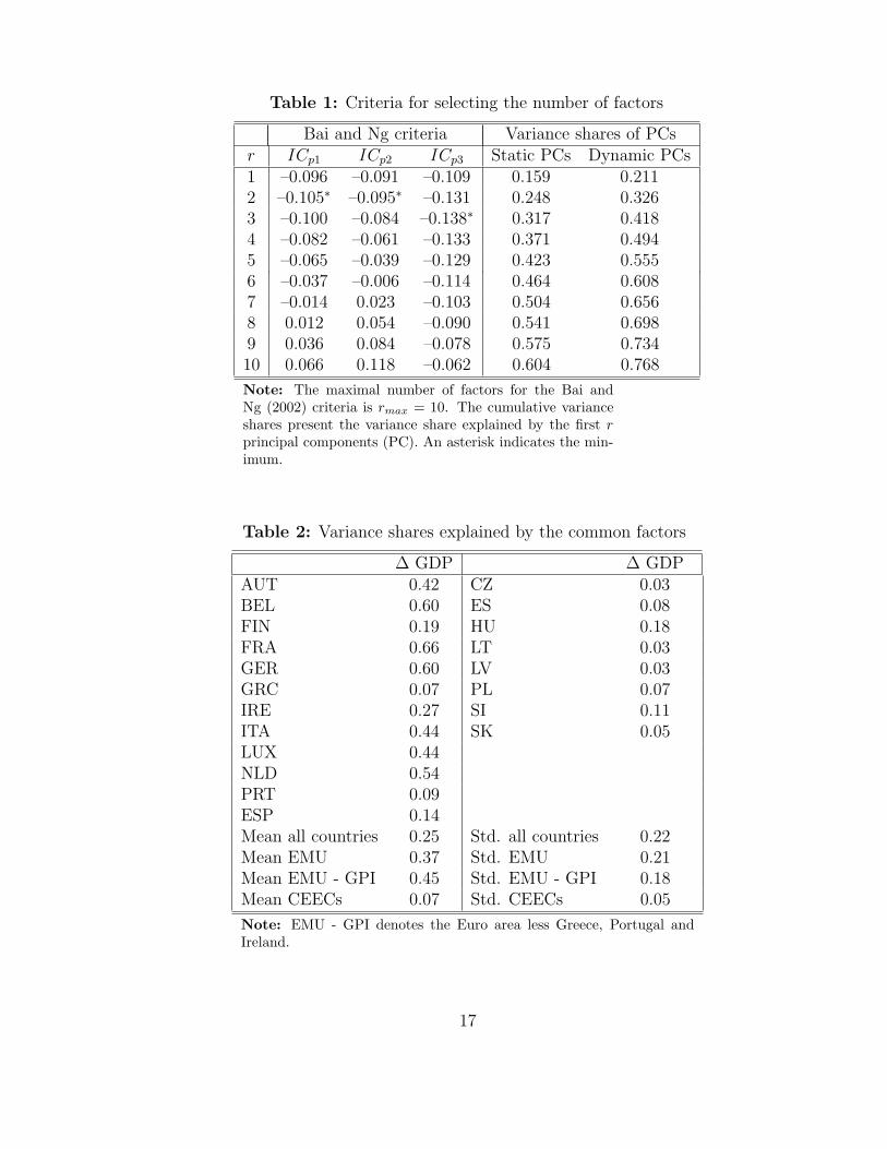
Table 1: Criteria for selecting the number of factors

Bai and Ng criteria Variance shares of PCsr ICp1 ICp2 ICp3 Static PCs Dynamic PCs1 –0.096 –0.091 –0.109 0.159 0.2112 –0.105∗ –0.095∗ –0.131 0.248 0.3263 –0.100 –0.084 –0.138∗ 0.317 0.4184 –0.082 –0.061 –0.133 0.371 0.4945 –0.065 –0.039 –0.129 0.423 0.5556 –0.037 –0.006 –0.114 0.464 0.6087 –0.014 0.023 –0.103 0.504 0.6568 0.012 0.054 –0.090 0.541 0.6989 0.036 0.084 –0.078 0.575 0.73410 0.066 0.118 –0.062 0.604 0.768

Note: The maximal number of factors for the Bai andNg (2002) criteria is rmax = 10. The cumulative varianceshares present the variance share explained by the first rprincipal components (PC). An asterisk indicates the min-imum.

Table 2: Variance shares explained by the common factors

∆ GDP ∆ GDPAUT 0.42 CZ 0.03BEL 0.60 ES 0.08FIN 0.19 HU 0.18FRA 0.66 LT 0.03GER 0.60 LV 0.03GRC 0.07 PL 0.07IRE 0.27 SI 0.11ITA 0.44 SK 0.05LUX 0.44NLD 0.54PRT 0.09ESP 0.14Mean all countries 0.25 Std. all countries 0.22Mean EMU 0.37 Std. EMU 0.21Mean EMU - GPI 0.45 Std. EMU - GPI 0.18Mean CEECs 0.07 Std. CEECs 0.05

Note: EMU - GPI denotes the Euro area less Greece, Portugal andIreland.

17

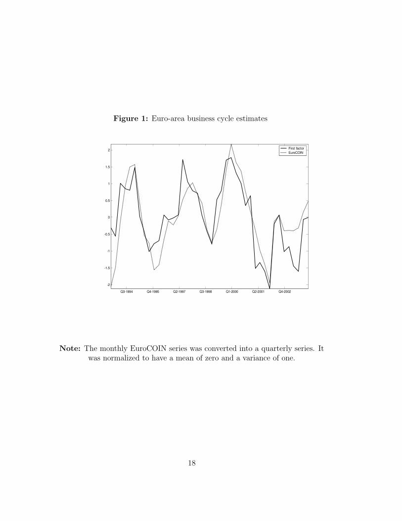
Figure 1: Euro-area business cycle estimates

Q3-1994 Q4-1995 Q2-1997 Q3-1998 Q1-2000 Q2-2001 Q4-2002

-2

-1.5

-1

-0.5

0

0.5

1

1.5

2 First factorEuroCOIN

Note: The monthly EuroCOIN series was converted into a quarterly series. Itwas normalized to have a mean of zero and a variance of one.

18

19

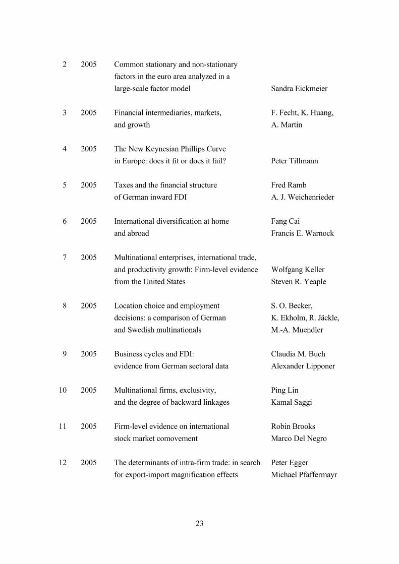
The following Discussion Papers have been published since 2004:

Series 1: Economic Studies

1 2004 Foreign Bank Entry into Emerging Economies: An Empirical Assessment of the Determinants and Risks Predicated on German FDI Data Torsten Wezel 2 2004 Does Co-Financing by Multilateral Development Banks Increase “Risky” Direct Investment in Emerging Markets? – Evidence for German Banking FDI Torsten Wezel 3 2004 Policy Instrument Choice and Non-Coordinated Giovanni Lombardo Monetary Policy in Interdependent Economies Alan Sutherland 4 2004 Inflation Targeting Rules and Welfare in an Asymmetric Currency Area Giovanni Lombardo 5 2004 FDI versus cross-border financial services: Claudia M. Buch The globalisation of German banks Alexander Lipponer 6 2004 Clustering or competition? The foreign Claudia M. Buch investment behaviour of German banks Alexander Lipponer 7 2004 PPP: a Disaggregated View Christoph Fischer 8 2004 A rental-equivalence index for owner-occupied Claudia Kurz housing in West Germany 1985 to 1998 Johannes Hoffmann 9 2004 The Inventory Cycle of the German Economy Thomas A. Knetsch 10 2004 Evaluating the German Inventory Cycle Using Data from the Ifo Business Survey Thomas A. Knetsch 11 2004 Real-time data and business cycle analysis in Germany Jörg Döpke

20

12 2004 Business Cycle Transmission from the US to Germany – a Structural Factor Approach Sandra Eickmeier 13 2004 Consumption Smoothing Across States and Time: George M. International Insurance vs. Foreign Loans von Furstenberg 14 2004 Real-Time Estimation of the Output Gap in Japan and its Usefulness for Inflation Forecasting and Policymaking Koichiro Kamada 15 2004 Welfare Implications of the Design of a Currency Union in Case of Member Countries of Different Sizes and Output Persistence Rainer Frey 16 2004 On the decision to go public: Ekkehart Boehmer Evidence from privately-held firms Alexander Ljungqvist 17 2004 Who do you trust while bubbles grow and blow? A comparative analysis of the explanatory power of accounting and patent information for the Fred Ramb market values of German firms Markus Reitzig 18 2004 The Economic Impact of Venture Capital Astrid Romain, Bruno van Pottelsberghe 19 2004 The Determinants of Venture Capital: Astrid Romain, Bruno Additional Evidence van Pottelsberghe 20 2004 Financial constraints for investors and the speed of adaption: Are innovators special? Ulf von Kalckreuth 21 2004 How effective are automatic stabilisers? Theory and results for Germany and other Michael Scharnagl OECD countries Karl-Heinz Tödter

21

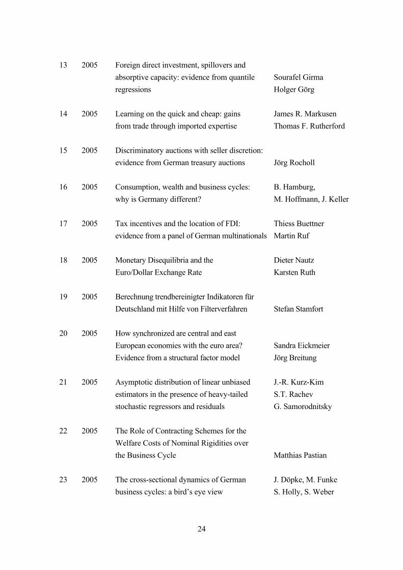
22 2004 Asset Prices in Taylor Rules: Specification, Pierre L. Siklos Estimation, and Policy Implications for the Thomas Werner ECB Martin T. Bohl 23 2004 Financial Liberalization and Business Cycles: The Experience of Countries in Lúcio Vinhas the Baltics and Central Eastern Europe de Souza 24 2004 Towards a Joint Characterization of Monetary Policy and the Dynamics of the Term Structure of Interest Rates Ralf Fendel 25 2004 How the Bundesbank really conducted Christina Gerberding monetary policy: An analysis based on Andreas Worms real-time data Franz Seitz 26 2004 Real-time Data for Norway: T. Bernhardsen, Ø. Eitrheim, Challenges for Monetary Policy A.S. Jore, Ø. Røisland 27 2004 Do Consumer Confidence Indexes Help Forecast Consumer Spending in Real Time? Dean Croushore 28 2004 The use of real time information in Maritta Paloviita Phillips curve relationships for the euro area David Mayes 29 2004 The reliability of Canadian output Jean-Philippe Cayen gap estimates Simon van Norden 30 2004 Forecast quality and simple instrument rules - Heinz Glück a real-time data approach Stefan P. Schleicher 31 2004 Measurement errors in GDP and Peter Kugler forward-looking monetary policy: Thomas J. Jordan The Swiss case Carlos Lenz Marcel R. Savioz

22

32 2004 Estimating Equilibrium Real Interest Rates Todd E. Clark in Real Time Sharon Kozicki 33 2004 Interest rate reaction functions for the euro area Evidence from panel data analysis Karsten Ruth 34 2004 The Contribution of Rapid Financial Development to Asymmetric Growth of Manufacturing Industries: George M. Common Claims vs. Evidence for Poland von Furstenberg 35 2004 Fiscal rules and monetary policy in a dynamic stochastic general equilibrium model Jana Kremer 36 2004 Inflation and core money growth in the Manfred J.M. Neumann euro area Claus Greiber 37 2004 Taylor rules for the euro area: the issue Dieter Gerdesmeier of real-time data Barbara Roffia 38 2004 What do deficits tell us about debt? Empirical evidence on creative accounting Jürgen von Hagen with fiscal rules in the EU Guntram B. Wolff 39 2004 Optimal lender of last resort policy Falko Fecht in different financial systems Marcel Tyrell 40 2004 Expected budget deficits and interest rate swap Kirsten Heppke-Falk spreads - Evidence for France, Germany and Italy Felix Hüfner 41 2004 Testing for business cycle asymmetries based on autoregressions with a Markov-switching intercept Malte Knüppel 1 2005 Financial constraints and capacity adjustment in the United Kingdom – Evidence from a Ulf von Kalckreuth large panel of survey data Emma Murphy

23

2 2005 Common stationary and non-stationary factors in the euro area analyzed in a large-scale factor model Sandra Eickmeier 3 2005 Financial intermediaries, markets, F. Fecht, K. Huang, and growth A. Martin 4 2005 The New Keynesian Phillips Curve in Europe: does it fit or does it fail? Peter Tillmann 5 2005 Taxes and the financial structure Fred Ramb of German inward FDI A. J. Weichenrieder 6 2005 International diversification at home Fang Cai and abroad Francis E. Warnock 7 2005 Multinational enterprises, international trade, and productivity growth: Firm-level evidence Wolfgang Keller from the United States Steven R. Yeaple 8 2005 Location choice and employment S. O. Becker, decisions: a comparison of German K. Ekholm, R. Jäckle, and Swedish multinationals M.-A. Muendler 9 2005 Business cycles and FDI: Claudia M. Buch evidence from German sectoral data Alexander Lipponer 10 2005 Multinational firms, exclusivity, Ping Lin and the degree of backward linkages Kamal Saggi 11 2005 Firm-level evidence on international Robin Brooks stock market comovement Marco Del Negro 12 2005 The determinants of intra-firm trade: in search Peter Egger for export-import magnification effects Michael Pfaffermayr

24

13 2005 Foreign direct investment, spillovers and absorptive capacity: evidence from quantile Sourafel Girma regressions Holger Görg 14 2005 Learning on the quick and cheap: gains James R. Markusen from trade through imported expertise Thomas F. Rutherford 15 2005 Discriminatory auctions with seller discretion: evidence from German treasury auctions Jörg Rocholl 16 2005 Consumption, wealth and business cycles: B. Hamburg, why is Germany different? M. Hoffmann, J. Keller 17 2005 Tax incentives and the location of FDI: Thiess Buettner evidence from a panel of German multinationals Martin Ruf 18 2005 Monetary Disequilibria and the Dieter Nautz Euro/Dollar Exchange Rate Karsten Ruth 19 2005 Berechnung trendbereinigter Indikatoren für Deutschland mit Hilfe von Filterverfahren Stefan Stamfort 20 2005 How synchronized are central and east European economies with the euro area? Sandra Eickmeier Evidence from a structural factor model Jörg Breitung 21 2005 Asymptotic distribution of linear unbiased J.-R. Kurz-Kim estimators in the presence of heavy-tailed S.T. Rachev stochastic regressors and residuals G. Samorodnitsky 22 2005 The Role of Contracting Schemes for the Welfare Costs of Nominal Rigidities over the Business Cycle Matthias Pastian 23 2005 The cross-sectional dynamics of German J. Döpke, M. Funke business cycles: a bird’s eye view S. Holly, S. Weber

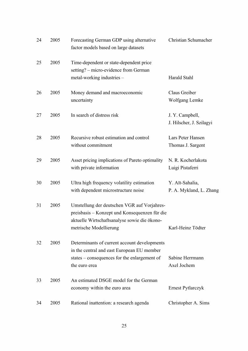
25

24 2005 Forecasting German GDP using alternative Christian Schumacher factor models based on large datasets 25 2005 Time-dependent or state-dependent price setting? – micro-evidence from German metal-working industries – Harald Stahl 26 2005 Money demand and macroeconomic Claus Greiber uncertainty Wolfgang Lemke 27 2005 In search of distress risk J. Y. Campbell, J. Hilscher, J. Szilagyi 28 2005 Recursive robust estimation and control Lars Peter Hansen without commitment Thomas J. Sargent 29 2005 Asset pricing implications of Pareto optimality N. R. Kocherlakota with private information Luigi Pistaferri 30 2005 Ultra high frequency volatility estimation Y. Aït-Sahalia, with dependent microstructure noise P. A. Mykland, L. Zhang 31 2005 Umstellung der deutschen VGR auf Vorjahres- preisbasis – Konzept und Konsequenzen für die aktuelle Wirtschaftsanalyse sowie die ökono- metrische Modellierung Karl-Heinz Tödter 32 2005 Determinants of current account developments in the central and east European EU member states – consequences for the enlargement of Sabine Herrmann the euro erea Axel Jochem 33 2005 An estimated DSGE model for the German economy within the euro area Ernest Pytlarczyk 34 2005 Rational inattention: a research agenda Christopher A. Sims

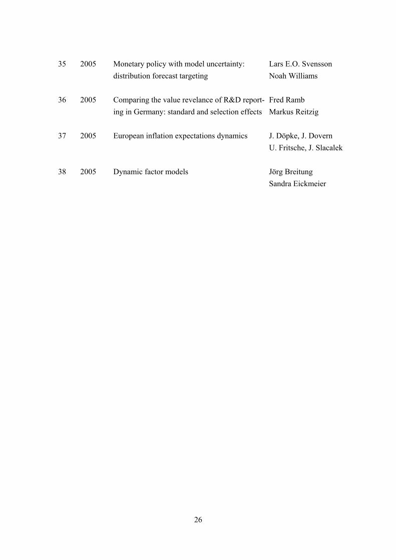
35 2005 Monetary policy with model uncertainty: Lars E.O. Svensson distribution forecast targeting Noah Williams 36 2005 Comparing the value revelance of R&D report- Fred Ramb ing in Germany: standard and selection effects Markus Reitzig 37 2005 European inflation expectations dynamics J. Döpke, J. Dovern U. Fritsche, J. Slacalek 38 2005 Dynamic factor models Jörg Breitung Sandra Eickmeier

26

27

Series 2: Banking and Financial Studies 1 2004 Forecasting Credit Portfolio Risk A. Hamerle, T. Liebig, H. Scheule 2 2004 Systematic Risk in Recovery Rates – An Empirical Analysis of US Corporate Klaus Düllmann Credit Exposures Monika Trapp 3 2004 Does capital regulation matter for bank Frank Heid behaviour? Evidence for German savings Daniel Porath banks Stéphanie Stolz 4 2004 German bank lending during F. Heid, T. Nestmann, emerging market crises: B. Weder di Mauro, A bank level analysis N. von Westernhagen 5 2004 How will Basel II affect bank lending to T. Liebig, D. Porath, emerging markets? An analysis based on B. Weder di Mauro, German bank level data M. Wedow 6 2004 Estimating probabilities of default for German savings banks and credit cooperatives Daniel Porath 1 2005 Measurement matters – Input price proxies and bank efficiency in Germany Michael Koetter 2 2005 The supervisor’s portfolio: the market price risk of German banks from 2001 to 2003 – Christoph Memmel Analysis and models for risk aggregation Carsten Wehn 3 2005 Do banks diversify loan portfolios? Andreas Kamp A tentative answer based on individual Andreas Pfingsten bank loan portfolios Daniel Porath 4 2005 Banks, markets, and efficiency F. Fecht, A. Martin

28

5 2005 The forecast ability of risk-neutral densities Ben Craig of foreign exchange Joachim Keller 6 2005 Cyclical implications of minimum capital requirements Frank Heid 7 2005 Banks’ regulatory capital buffer and the business cycle: evidence for German Stéphanie Stolz savings and cooperative banks Michael Wedow 8 2005 German bank lending to industrial and non- industrial countries: driven by fundamentals or different treatment? Thorsten Nestmann 9 2005 Accounting for distress in bank mergers M. Koetter, J. Bos, F. Heid C. Kool, J. Kolari, D. Porath 10 2005 The eurosystem money market auctions: Nikolaus Bartzsch a banking perspective Ben Craig, Falko Fecht 11 2005 Financial integration and systemic Falko Fecht risk Hans Peter Grüner

Visiting researcher at the Deutsche Bundesbank

The Deutsche Bundesbank in Frankfurt is looking for a visiting researcher. Visitors shouldprepare a research project during their stay at the Bundesbank. Candidates must hold aPh D and be engaged in the field of either macroeconomics and monetary economics,financial markets or international economics. Proposed research projects should be fromthese fields. The visiting term will be from 3 to 6 months. Salary is commensurate withexperience.

Applicants are requested to send a CV, copies of recent papers, letters of reference and aproposal for a research project to:

Deutsche BundesbankPersonalabteilungWilhelm-Epstein-Str. 14

D - 60431 FrankfurtGERMANY

29 31